HAL Id: hal-00644154https://hal.archives-ouvertes.fr/hal-00644154

Submitted on 23 Nov 2011

HAL is a multi-disciplinary open accessarchive for the deposit and dissemination of sci-entific research documents, whether they are pub-lished or not. The documents may come fromteaching and research institutions in France orabroad, or from public or private research centers.

L’archive ouverte pluridisciplinaire HAL, estdestinée au dépôt et à la diffusion de documentsscientifiques de niveau recherche, publiés ou non,émanant des établissements d’enseignement et derecherche français ou étrangers, des laboratoirespublics ou privés.

Adaptive Observer Design under Low Data RateTransmission with Applications to Oil Well Drill-string

Rafael Barreto Jijon, Carlos Canudas de Wit, Silviu-Iulian Niculescu,Jonathan Dumon

To cite this version:Rafael Barreto Jijon, Carlos Canudas de Wit, Silviu-Iulian Niculescu, Jonathan Dumon. AdaptiveObserver Design under Low Data Rate Transmission with Applications to Oil Well Drill-string. Amer-ican Control Conference (ACC2010), Jun 2010, Baltimore, Maryland, United States. pp.1973-1978,2010. <hal-00644154>

Adaptive Observer Design under Low Data Rate Transmission withApplications to Oil Well Drill-string

Rafael Barreto Jijon, Carlos Canudas-de-Wit, Silviu-Iulian Niculescu, Jonathan Dumon

Abstract— In oil well drilling operations, one of the importantproblem to deal with is represented by the necessity of sup-pressing harmful stick-slip oscillations. A control law namedD-OSKIL mechanism uses the weight-on-the-bit force as acontrol variable to extinguish limit cycles. It uses the valueof the bit angular velocity that is found through an unknownparameter observer by means of the measure of the table rotaryangular speed. To improve this former estimation, we add themeasurement of the angular velocity of the bit that, due tothe technological constraints, arrives delayed. This new designleads us to the analysis of a time-varying delay system.

Index Terms— Stick-Slip, Oil Well drill string, D-OSKIL,unknown parameter adaptive observer, time-variant, delay,stability.

I. INTRODUCTION

Oil well drilling operations present a particular frictionphenomenon called Stick-Slip Oscillations which consists ina sub-normal irregular rotation movement, e.g., the top of thedrill string rotates with a constant angular velocity, mean-while downhole, the bit (cutting device) angular velocityvaries in a range from zero to six times the one measuredat the surface. This effect appears mainly when the bit is incontact with rock formations [1],[10].

Due to the very large forces that are applied into thebit, the presence of stick-slip self-excited oscillations cancause irreversible damage to the equipment, as for example,shut-downs, operation delays, decreasing service life of drillstrings and downhole equipment. Since avoiding this kindof oscillations can provide important savings in terms ofexploitation time, spare parts costs and maintenance this taskhas become a challenge for drillers and scientists. Furtherdetails about stick-slip and drilling oscillations can be foundin [19], [2], [14] and [17].

A model for the drill string system and for the stick-slip oscillations as well as an appropriate control law calledDrilling-Oscillation Killer (D-OSKIL) have been proposedin [3]. The controller uses mainly a vertical force sometimesnamed “weight on the bit” (WoB) as an additional variableto eliminate stick-slip effects. Additionally, not all the valuesof the states of the system are available for control. Adaptiveobserver has been designed to provide an estimation of such

R. Barreto Jijon is with the INPG, GIPSA-Lab, NeCS team. Grenoble,France. (e-mail: rafael.barreto.jijon@gmail.com)

C. Canudas-de-Wit is with the CNRS, GIPSA-Lab, NeCS team. Grenoble, France. (e-mail:carlos.canudas-de-wit@gipsa-lab.inpg.fr)

S.-I. Niculescu is with the L2S, CNRS-Supelec, Gif-sur-Yvette, France.(e-mail: Silviu.Niculescu@lss.supelec.fr)

J. Dumon is with the CNRS, GIPSA-Lab, NeCS team. Grenoble, France.(e-mail: jonathan.dumon@gipsa-lab.inpg.fr)

states and, additionally, to estimate the friction coefficient. Inthis case, the measured variable is the rotary angular speed.

Since the physics effects occurring downhole have nostrong influence at surface due to the attenuation along thedrill string, the measurement does not effectively reflectthem. This means that the signal to noise ratio is small andit affects the quality of estimation. We are to improve theobserver’s behavior, using some coarse information comingfrom the drilling toll with a new measurement: the bit angularvelocity. As explained in the forthcoming section, the tech-nological constraints induce the presence of a transmissiondelay. It is worth to mention that such a delay introduces anadditional difficulty in the control problem as pointed out inthe literature in different other cases [8], [16], [13]

The paper is organized as follows: In section II, we brieflyintroduce the model of the dynamical system along witha description of the testbed where the observer is to beimplemented as well as some operational conditions. SectionIII includes some discussions on the particular physicalconstraints as well as the technological feasibility of theimplementation of the observer. In section IV we tacklethe observer’s development and its stability conditions andfinally, some concluding remarks in section VI end the paper.

Throughout the paper, the following notations will beused: the space C v

n,τ is a set defined by {φ ∈Cn,τ : ‖φ‖c < v}where Cn,τ = C ([−τ,0],Rn) represents the Banach space ofthe definite piecewise-continuous vector functions mappingthe interval [−τ,0] into Rn with the uniform convergencetopology, and

‖φ‖c = sup−τ≤t≤0

‖φ(t)‖

represents the norm of the function φ ∈ Cn,τ .

II. SYSTEM DESCRIPTION

A. Model

The system is modeled as two coupled masses as shown inFigure 1. Jr and Jb are two inertial masses locally damped bydr and db. The inertias are coupled through an elastic shaft ofstiffness k and damping c. Let us define ϕr, ϕb as the angularpositions of the rotary and the bit respectively; ϕr, ϕb astheir angular velocities, u(t) = WoB is the weight on the bitcontrol signal, v(t) is the rotary table torque control signalused to regulate ϕr, µ is the friction coefficient; A, B, H, Coare model matrices given in (3), Ψ(t) = Ψ(u(t)) = Hu(t), xis the state vector and yo is the output variable. For a moredetailed description, see, for instance, [3].

Fig. 1. Drill string two-coupled masses model.

The model to be used is described by:

x(t) = Ax(t)+Bv(t)+Ψ(t)µ (1)yo = Co x = ϕr,

where the state x = [x1 x2 x3]T is defined as follows:

x1 = ϕr−ϕb, x2 = ϕr, x3 = ϕb (2)

and

A =

0 1 −1− k

Jr− dr+c

JrcJr

kJb

cJb

− c+dbJb

, B =

01Jr0

H =

00− 1

Jb

, Co =(

0 1 0)

(3)

B. Testbed

In order to validate the proposed results, an appropriatetestbed has been built. It is shown in Figure 2 as well as itsschematic in Figure 3. It has a Host PC for development,compiling and user interface. A target PC is also used forreal-time execution of the code like the observer and the D-OSKIL controller [12]. The rotary system is composed ofa DC motor, a transmission box, the rotary table, the drillstring, a bit and a quadrature encoder. The support platformconsists of a DC motor to move the rotary system vertically,a specimen holder, a support structure and a tension forcesensor. The acoustic signal is simulated as sonar pulseslike a beeper and microphone pear as shown in Figure 3.Furthermore, the delay is added artificially by software.

We will define the following operation conditions: Welldepth: d ∈ [0,8000] meters, since drilling penetration speedis usually very small, we can consider it as negligible: d ≈ 0.In practice, we have found that ϕb ∈ [0,31] rad/s with typicalvalue ϕb = 5 rad/s.

Fig. 2. Experimental setup

Fig. 3. Testbed schematic with sonar pulses

III. WIRELESS-TRANSMISSION TECHNOLOGIES

In this section, we focus on the way to bring the mea-surement from downhole to surface so we can use it forimproving the observer’s behavior.

There are mainly two types of transmission: throughtelemetry signals along the drilling fluid often referred to asmud-pressure pulses [9] and through acoustic waves alongthe drillstring [4].

In most of the literature, electronic equipments are de-signed for data acquisition and to play the modulator roll. Itshould be implemented as an autonomous system energizedeither by a mud operated electrical turbine or by a batterypack [18].

A. Mud-pulse telemetry

This technology uses the mud that goes through thedrilling system as a transmission media. The data will berepresented by pressure pulses. According to [18], the pulseractuator (a stepper-motor-based device) and a main valverestricts the flow and creates some pressure-pulse sequence.A piezoelectric device captures these variations that are thenanalyzed by a micro-controller. Evidently, due to the irregularnature the mud flow, the low frequency vibrations producedby mud pumps and pulsation dampeners the signals arecorrupted by noise. Furthermore, they have an important

attenuation. Some characteristics to highlight are [11], [4],[7] its cost-effective data transfer, its very low bite rate (1or 2 bits per second). Mud-pulse velocity declines with thedisturbances of mud density, gas content and mud compress-ibility. It becomes more difficult with increasing well depth.Pulse waves travel through the borehole at 1200 meters persecond [11], hence the measure arrives with some delay thatincreases up to τmax ≈ 6.6 seconds .

B. Acoustic data transmission over a drill string

Since the acoustic wave propagation velocity in the stringmaterial is at least three times superior to that in the mud ofthe borehole [4], and a higher transmission rate is possible(typically 6 bps), acoustic transmission seems to be the bestway to emit pulses to the surface. These acoustic wavesare generated torsional contractions generated by magnetorestrictive rings set inside the pipe [6]. In this case τmax≈ 2.2.It is useful to note that there exists an attenuation of around4 dB/300m [5]. However, we can neglect it because thereis always a possibility of setting a repeater at any joint ateach 10-15 meters of the section. We consider that this factdoes not add any extra considerable delay since the repeater’samplification can occur almost instantaneously.

The telemetry system sends signals directly to the surfacethrough the channel. Usually, there is an embedded sensormeasuring ϕb downhole. A measurement noise S(t) is addedto the data and then coded all together in such a way it canbe transmitted through the acoustic channel G. At surface,a receiver will read the encoded signal with the noise N(t).Furthermore, a digital algorithm is used to decode this dataand make it available for the use of the observer. Bothmethods can be modeled by the schematic shown in Figure4.

Fig. 4. Block diagram of the transmission channel.

C. Transmission delay range and friction hypothesis

Due to technical considerations we can assume that thetransmission media is, as a first approximation, like a puredelay system with delay time τ ∈ [0,τmax]. Moreover, thewell’s depth increases at a very slow rate and it stops each 10-15 meters. In this procedure, the delay can be recalculated.Hence, the delay can be defined as a constant, that is τ = 0.

On the other hand, we will consider that the frictioncoefficient is constant or at least slow time variant µ ≈0. This approximation is often assumed in the context ofadaptive control. This hypothesis means that the rate ofvariation of the rock friction coefficient does not exhibitsubstantial changes during drill-operation. Even if the drilledsurfaces may have different friction characteristics, the rateof penetration remains small (d ≈ 0).

IV. ADAPTIVE OBSERVER DESIGN WITH DELAYEDFEEDBACK SIGNALS

A general architecture is proposed in Figure 5 where Σ isthe system model, Σ is the observer, x is the observed statevector, Ko is the default observer gain, Km is the observergain when the value of ϕb becomes available and G is thetransmission channel. Here the outputs of the system arey1 = ϕr, and y2 = ϕb.

Fig. 5. General Architecture

A. Main Results

In this section, we will focus on a particular extensionof the original observer designed in [3] to handle the delaypresence and noise requirements. In this sense, we add twogains related to the delayed measurement as follows:

˙x(t) = Ax(t)+Bv(t)+Ψ(t)µ(t)+[K +βΓ(t)ΓT (t)CT

o ][yo(t)−Cox]+Kx[ym(t− τ)−Cmx(t− τ)] (4)

˙µ(t) = βΓT (t)CT

o [yo(t)−Cox]+Kµ [ym(t− τ)−Cmx(t− τ)] (5)

Γ(t) = (A−KCo)Γ(t)+Ψ(t) (6)

where, ym(t − τ) is the new delayed output vector,Cm ∈R1×3, Kx ∈R3 and Kµ ∈R are the output matrix, andgain matrices for the delayed measurement. Γ(t) ∈ R3 is amatrix generated by the system free of delay (6) such thatit generates the states dependent of µ . Here, β is a positivescalar and v(t) (and then Ψ(t)) is persistently exciting, forexample ∃δ ,T > 0 such that the following inequality holds:∫ t+T

tΓ

T (ξ )CTo CoΓ(ξ )dξ > δ > 0 (7)

Theorem 1. The unknown parameter adaptive observerdescribed by (4)-(6) guarantees exponential stability forsmall delays τ ∈ [0, τ) if there exists some gain matricesKx and Kµ such that

Kx(t) = Γ(t)Kµ (8)

and the following conditions hold simultaneously:

(i) (A−KCo) is Hurwitz, and(ii) the inequalities

0 < amin−KµCmΓ∗ (9)

τ < τ = 2amin−KµCmΓ∗

| KµCmΓ∗ | (2 | KµCmΓ∗ |+1+a2max)

, (10)

with:

amin = mint≥0

(βΓT (t)CT

o CoΓ(t)),

amax = maxt≥0

(βΓT (t)CT

o CoΓ(t)).

Proof 1. Following the method described in [20] with theconstraint (11), we introduce (5) into (4) and then we havethe expression of the system (12).

Kx(t) = Γ(t)Kµ (11)˙x(t) = Ax(t)+Bv(t)+Ψ(t)µ(t)

+K(yo(t)−Cox(t))+Γ(t) ˙µ(t) (12)

Let x(t) = x(t)−x(t), µ(t) = µ(t)−µ with µ = 0 and since˙µ(t) = ˙µ(t)− µ we obtain:

˙x(t) = (A−KCo)x(t)+Ψ(t) ˙µ(t)+Γ(t) ˙µ(t) (13)

We define the following variable transformation:

η(t) = x(t)−Γ(t)µ(t) (14)

then we obtain:

η(t) =(A−KCo)(η(t)+Γ(t)µ(t))+Ψ(t)µ(t)− Γ(t)µ(t)=(A−KCo)η(t)

+ [(A−KCo)Γ(t)+Ψ(t)− Γ(t)]µ(t)

Due to the system (6), we have:

η(t) = (A−KCo)η(t). (15)

The system (15) can be assumed as strictly stable e.g. theconstant pair (A−KCo) is detectable. Now, we will focus onanalyzing the behavior of µ:

˙µ(t) = βΓT (t)CT

o (yo(t)−Cox(t))+KµCmx(t− τ)

=−βΓT (t)CT

o Cox(t)+KµCmx(t− τ)

=−βΓT (t)CT

o Co(η(t)+Γ(t)µ(t))+KµCmx(t− τ)(16)

Sincex(t− τ) = η(t− τ)+Γ(t− τ)µ(t− τ)

then

˙µ(t) = −βΓT (t)CT

o Co(η(t)+Γ(t)µ(t))+KµCm[η(t− τ)+Γ(t− τ)µ(t− τ)]

Define now:

a(t) = βΓT (t)CT

o CoΓ(t) (17)b(t) = −KµCmΓ(t− τ) (18)

where 0≤ a(t)≤maxt≥0 (a(t)) = amax and b(t) are scalars.On the other hand, we can approximate

Γ∗(t) =−(A−KCo)−1

Ψ∗(t) =−(A−KCo)−1Hu∗(t)

where Γ∗, Ψ∗ and u∗ denote the steady state of Γ(t), Ψ(t) andu(t) respectively. Physically, u(t) is a vertical force movingheavy rotating masses with friction. Thus, this movement cannot be neither so fast nor sudden. Therefore, we can considerthat u∗ and then Γ∗ vary slowly and they can be treated asconstants. Since µ changes faster than the variability of thegain, we can assume b(t)≈−KµCmΓ∗ , b.Then

˙µ(t) =−a(t)µ(t)−bµ(t− τ)+ f [η(t),η(t− τ)] (19)

Summarizing, we start with the autonomous system η . Weget an adaptation equation by injecting it into that of ˙µ . Withthese “present” and “past” values we compute a estimation ofthe state vector. The development of the observer’s equationsare resumed in Figure 6: Since f [η(t),η(t− τ)]→ 0 while

Fig. 6. Observer’s equation development Block Diagram

t → ∞ the problem becomes, at the next step, by analyzingthe homogenous part of the equation, to find conditions suchthat system ˙µ(t) = −a(t)µ(t)− bµ(t − τ) is exponentiallystable, and then explicitly compute the gains. For sake ofwriting simplicity let us define χ(t) = µ(t). Then the systembecomes:

χ(t) =−a(t)χ(t)−bχ(t− τ) (20)

We have the following result (see the appendix for the proof):Lemma 2. The time variant delay system described by

(20) is asymptotically stable for all τ ∈ [0, τ) if the followingconditions hold:

amin +b > 0 (21)

τ < 2amin +b

2b2 +(a2max +1) | b |

(22)

Hence, if there exists ε > 0, τ > 0 and amax > 0, amin ≥ 0verifying the conditions in Lemma 2, it is possible to designa gain b > 0 that makes system (20) asymptotically stable.

Let σ ,ε,λ three positive scalars. We know that

0 < σ‖χ(t)‖2 ≤V (χt)V (χt) ≤−ε‖χ(t)‖2 ≤ 0,

where V represents the Lyapunov-Krasovskii functional al-lowing us to conclude on the exponential stability of (20):

V (χt)V (χt)

≤− ε

σ

integrating in a positive sense we get:∫ t

0

V (χρ))V (χρ))

dρ ≤∫ t

0− ε

σdρ

(23)

Finally, we obtain:

V (χt) ≤ λe−εσ

t (24)

This means that V (χt) decreases exponentially, that impliesthat the system converges to zero exponentially fast. Thus, ifthe conditions shown above are held, the system is globallyexponentially stable.

This concludes proofs of theorems 1 and 2.

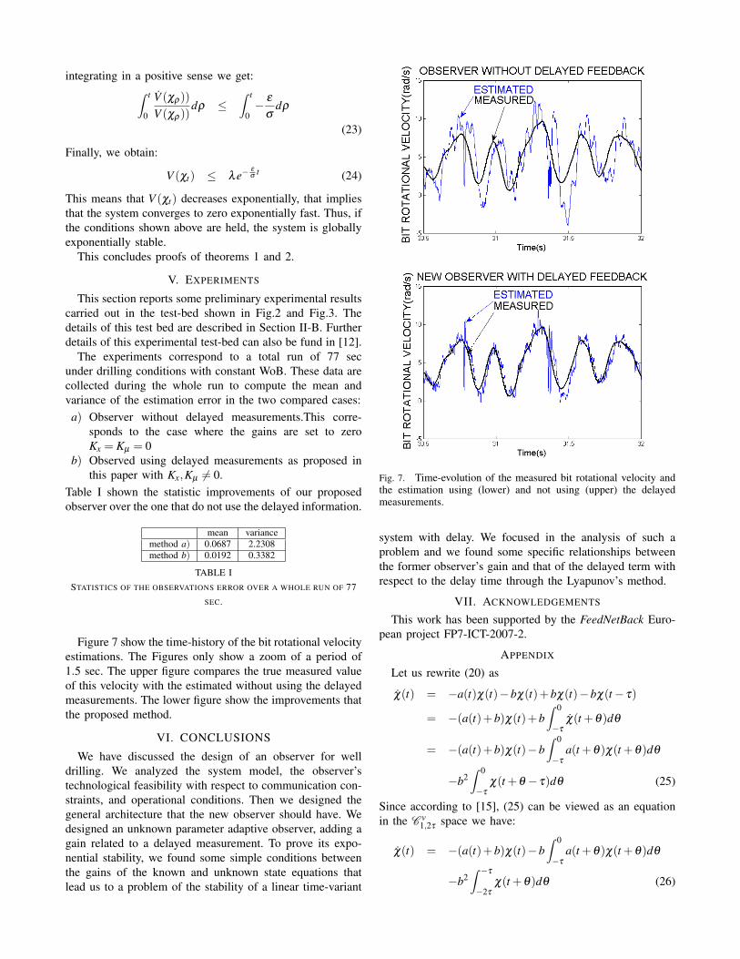
V. EXPERIMENTS

This section reports some preliminary experimental resultscarried out in the test-bed shown in Fig.2 and Fig.3. Thedetails of this test bed are described in Section II-B. Furtherdetails of this experimental test-bed can also be fund in [12].

The experiments correspond to a total run of 77 secunder drilling conditions with constant WoB. These data arecollected during the whole run to compute the mean andvariance of the estimation error in the two compared cases:a) Observer without delayed measurements.This corre-

sponds to the case where the gains are set to zeroKx = Kµ = 0

b) Observed using delayed measurements as proposed inthis paper with Kx,Kµ 6= 0.

Table I shown the statistic improvements of our proposedobserver over the one that do not use the delayed information.

mean variancemethod a) 0.0687 2.2308method b) 0.0192 0.3382

TABLE ISTATISTICS OF THE OBSERVATIONS ERROR OVER A WHOLE RUN OF 77

SEC.

Figure 7 show the time-history of the bit rotational velocityestimations. The Figures only show a zoom of a period of1.5 sec. The upper figure compares the true measured valueof this velocity with the estimated without using the delayedmeasurements. The lower figure show the improvements thatthe proposed method.

VI. CONCLUSIONS

We have discussed the design of an observer for welldrilling. We analyzed the system model, the observer’stechnological feasibility with respect to communication con-straints, and operational conditions. Then we designed thegeneral architecture that the new observer should have. Wedesigned an unknown parameter adaptive observer, adding again related to a delayed measurement. To prove its expo-nential stability, we found some simple conditions betweenthe gains of the known and unknown state equations thatlead us to a problem of the stability of a linear time-variant

Fig. 7. Time-evolution of the measured bit rotational velocity andthe estimation using (lower) and not using (upper) the delayedmeasurements.

system with delay. We focused in the analysis of such aproblem and we found some specific relationships betweenthe former observer’s gain and that of the delayed term withrespect to the delay time through the Lyapunov’s method.

VII. ACKNOWLEDGEMENTS

This work has been supported by the FeedNetBack Euro-pean project FP7-ICT-2007-2.

APPENDIX

Let us rewrite (20) as

χ(t) = −a(t)χ(t)−bχ(t)+bχ(t)−bχ(t− τ)

= −(a(t)+b)χ(t)+b∫ 0

−τ

χ(t +θ)dθ

= −(a(t)+b)χ(t)−b∫ 0

−τ

a(t +θ)χ(t +θ)dθ

−b2∫ 0

−τ

χ(t +θ − τ)dθ (25)

Since according to [15], (25) can be viewed as an equationin the C v

1,2τspace we have:

χ(t) = −(a(t)+b)χ(t)−b∫ 0

−τ

a(t +θ)χ(t +θ)dθ

−b2∫ −τ

−2τ

χ(t +θ)dθ (26)

Let us define a Lyapunov-Krasovskii functional candidateV (χt) of the form

V (χt) = V1(χ(t))+V2(χt)+V3(χt), (27)

with:

V1(χ(t)) =12

χ(t)2 ≥ 0 (28)

V2(χt) =12

b2∫ −τ

−2τ

∫ t

t+θ

χ(ξ )2dξ dθ ≥ 0 (29)

V3(χt) =12

a2max | b |

∫ 0

−τ

∫ t

t+θ

χ(ξ )2dξ dθ ≥ 0 (30)

We take the derivative of V1(χ(t)) along the system (20):

V1(χ(t)) =− (a(t)+b)χ(t)2

−b∫ 0

−τ

χ(t)a(t +θ)χ(t +θ)dθ

−b2∫ −τ

−2τ

χ(t)χ(t +θ)dθ

Since we know that:

−b2∫ −τ

−2τ

χ(t)χ(t +θ)dθ ≤ 12

b2τχ(t)2

+12

b2∫ −τ

−2τ

χ(t +θ)2dθ (31)

we can rewrite V1 as:

V1(χ(t)) ≤ −(a(t)+b)χ(t)2

−b∫ 0

−τ

χ(t)a(t +θ)χ(t +θ)dθ +12

b2τχ(t)2

+12

b2∫ −τ

−2τ

χ(t +θ)2dθ

Let us find the derivative of V2 as:

V2(χt) =12

b2τχ(t)2− 1

2b2∫ −τ

−2τ

χ(t +θ)2dθ (32)

Finally,

V3(χt)≤12| b | a2

maxτχ(t)2− 12| b | a2

max

∫ 0

−τ

χ(t +θ)2dθ

Finally, adding all Lyapunov-candidates and using the prop-erty that 0≤ amin ≤ a(t)≤ amax, it follows that

V (χ(t)) = V1(χ(t))+V2(χ(t))+V3(χ(t))

≤−(amin +b−b2τ− | b | a

2max

2τ− | b |

2τ)χ(t)2

≤−εχ(t)2 (33)

where ε > 0.Hence, according to the Lyapunov-Krasovskii theorem, we

need to find a condition for (33) to be negative definite sowe can have asymptotic stability for the system (20):

0 < amin +b

(a2max +1+2 | b |) | b | τ < 2(amin +b)

This concludes the proof.

REFERENCES

[1] B. Armstrong-Helouvry. Stick-slip arising from stribeck friction. Proc.IEEE Int. Conf. Robot. Autom., 2:1377–1382, 1990.

[2] A. Baumgart. Stick-slip and bit-bounce of deep-hole drillstrings. J.Energy Resour. Technol., 122, 2000.

[3] C. Canudas-de Wit, F. Rubio, and M. A. Corchero. D-OSKIL: Anew mechanism for controlling Stick-Slip Oscilations in oil welldrillstrings. IEEE Trans. Control Sys. Tech., 16:1177–1191, November2008.

[4] F. Clayer, H. Heneusse, and J. Sancho. Procede de transmissionacoustique de donnees de forage d’un puits. In World IntellectualProperty Organization, March 1992. No. WO 92/04644.

[5] D. Drumheller. Acoustical properties of drill strings. Sandia NationalLaboratories Research Report, December 1988.

[6] D. Drumheller. An overview of acoustic telemetry. Sandia NationalLaboratories Research Report, December 1992.

[7] D. Drumheller and S. Knudsen. The propagation of sound waves indrill strings. J. Acoustical Society of America, 97(4):2116–2125, April1995.

[8] K. Gu, V. L. Kharitonov, and J. Chen. Stability of time-delay systems.Birkhauser, 2003.

[9] B. Jeffryes, K. Moriarty, and S. Reyes. Method and apparatus forenhanced acoustic mud-pulse telemetry. In World Intellectual PropertyOrganization, September 2001. No. WO 01/66912 A1.

[10] A. Kyllingstad and G. W. Halsey. A study of stick/slip motion of thebit. SPE Drilling Eng., 3-4:369–373, 1988.

[11] X. Liu, B. Li, and Y. Yue. Transmission behavior of mud-pressurepulse along well bore. Journal of Hydrodinamics, 19(2):236–240,2007.

[12] H. Lu, J. Dumon, and C. Canudas-de Wit. Experimental study of theD-OSKIL mechanism for controlling the stick-slip oscillations in adrilling labratory testbed. IEEE Multiconf. Systems and Control, StPetersburg:Russian Federation, 2009.

[13] W. Michiels and S.-I. Niculescu. Stability and stabilization of time-delay systems. An eigenvalue based approach. SIAM, 2007.

[14] E.M. Navarro-Lopez and Suarez-Cortez. Vibraciones mecanicas enuna sarta de perforacion: Problemas de control. Revista Iberoameri-cana de Automatica e Informatica Industrial, 2:43–54, Jan 2005.

[15] S. Niculescu. Sytemes a retard. Diderot, 1997.[16] S.-I. Niculescu. Delay effects on stability. A robust control approach.

Springer-Verlag, LNCIS, vol. 269, 2001.[17] P.D. Spanos, A.M. Chevalier, N.P. Politis, and N.L. Payne. Oil well

drilling: A vibrations perspective. Shock Vibration Dig, 35(2):81–99,2003.

[18] P. Tubei, C. Bergeron, and S. Bell. Mud-pulser telemetry system fordown hole Measurement-While-Drilling. In IEEE 9th Proc. Instrumentand Measurement Tech. Conf., pages 219–223, May 1992.

[19] M. Zamanian, S.E. Kadem, and M.R. Ghazavi. Stick-slip oscillationsof drag bits by considering damping of drilling mud and activedamping system. J. of Petroleum Science and Eng., 59:289–299, 2007.

[20] Q. Zhang. Adaptive observer for MIMO linear time varying systems.INRIA Rennes Research Report, January 2001.