ARTICLE IN PRESS

Neurocomputing 73 (2009) 461–467

Contents lists available at ScienceDirect

Neurocomputing

0925-23

doi:10.1

� Corr

E-m1 Th2 Th

journal homepage: www.elsevier.com/locate/neucom

Adaptive output-feedback decentralized control of a class of second ordernonlinear systems using recurrent fuzzy neural networks

Miguel Hernandez �,1, Yu Tang 2

Faculty of Engineering, National University of Mexico, Mexico City, Mexico

a r t i c l e i n f o

Article history:

Received 24 June 2008

Received in revised form

6 March 2009

Accepted 8 July 2009

Communicated by M.-J. Ercomponent aimed at compensating for the interconnections. Finally, an adaptive output-feedback

Available online 7 August 2009

Keywords:

Adaptive decentralized control

Recurrent neural fuzzy networks

Output-feedback

Lyapunov stability

12/$ - see front matter & 2009 Elsevier B.V. A

016/j.neucom.2009.07.010

esponding author. Tel.:+52 55 56234142.

ail address: juriqui@yahoo.com.mx.

e work of Miguel Hernandez is supported by

is work is partly supported by PAPIIT-IN1200

a b s t r a c t

In this paper the design of an adaptive output-feedback decentralized control for the class of second

order nonlinear affine interconnected systems based on recurrent fuzzy neural networks (RFNN) is

addressed. First, a centralized control that needs the state measurements of all subsystems is designed.

Then a decentralized control using the local state measurements is obtained by adding a control

decentralized control based on an RFNN is designed. In design of such controller, no separated state

estimator is needed, since the controller dynamics is embedded in the recurrent network. Practical

tracking is established by invoking Lyapunov stability analysis. Simulation and experimental results are

presented to evaluate the performance of the proposed control law.

& 2009 Elsevier B.V. All rights reserved.

1. Introduction

Control design for the class of second order affine nonlinearinterconnected systems may arise from applications of robotcontrol, servo applications, power system, and civil structurecontrol (see, e.g., [12,13] and the references cited therein), tomention just few of them. An important challenge in dealing withthis class of systems is the uncertainties in them, specially in theinterconnections. Decentralized control provides an alternative tothis challenge, because of its advantages such as design simplicity,computational efficiency, robustness to failures, scalability, andcapability of achieving a similar performance as in a centralizedcontrol under certain conditions [13].

In [5] it was proposed a model reference adaptive controlbased on the matrix-M condition [7], which requiresthe interconnection to be dominated by the local stability margin.Later, [2] eliminated this requirement by assuming thatthe interconnections enter by the same channel as thecontrol signal (Matching condition). Shi and Singh [14] and Tanget al. [19] proposed a scheme in which the interconnection isassumed to be bounded by a polynomial of high order in statevariables.

ll rights reserved.

CONACyT, Mexico.

09 UNAM.

Fuzzy logic system and neural networks have shown to beefficient tools for control system designs [17,11,22,9,16,21]. Byintroducing feedback links and combining the advantages of fuzzylogic systems and neural networks, recurrent fuzzy-neural net-works (RFNNs) have been created and considered to have animproved capability for identification and control of nonlineardynamic systems than networks without recurrence [3,6].Recently, decentralized control designs based on RFNNs havebeen proposed in [4,20,1]. In these works, a general nonlinearaffine system is considered. In [4], Huang et al. designed anindirect fuzzy control. Using a recurrent high-order networks,Benitez et al. designed a variable structure neural control for theclass of block-controllable nonlinear systems [1]. These controlimplementations require the full local state information. Bymeans of a state observer, Tong et al. [20] gave an adaptive fuzzycontrol scheme, both direct and indirect, which uses only the localoutput for the feedback.

In this paper the design of an adaptive output-feedbackdecentralized control for the class of second order nonlinearaffine interconnected systems based on RFNNs is addressed. First,a centralized control that needs the state measurements of allsubsystems is designed. Then a decentralized control using thelocal state measurements is obtained by adding a controlcomponent aimed at compensating for the interconnections.Finally, an adaptive output-feedback decentralized control basedon an RFNN is designed. In the design of such controller, noseparated state estimator as in [20] is needed, since the controllerdynamics is embedded in the recurrent network. Practicaltracking is established by invoking Lyapunov stability analysis.

ARTICLE IN PRESS

M. Hernandez, Y. Tang / Neurocomputing 73 (2009) 461–467462

Simulation in two coupled pendulums and experiment in a twodegree-of-freedom (DOF) robot are presented to evaluate theperformance of the proposed control law.

The main difference between the results in this paper andthose in our previous work [19] is the approach taken to solve thedecentralized control problem. In [19] adaptive control based onsliding mode was used to design a decentralized state feedbackcontrol for Lagrangian interconnected systems, whereas in thispaper an output-feedback decentralized control based on an RFNNwith on-line tuning consequent parameters is designed. The restof the paper is organized as follows: Section 2 gives the problemstatement, Section 3 describes the recurrent fuzzy-neural networkused for controller implementation. In Section 4, the design of thedecentralized control is proceeded by first designing an idealcentralized control that uses the state measurements of the wholesystem, then by adding a compensation signal in the control, anideal decentralized control using only local state measurements isconsidered. Lastly, based on the RFNN described in Section 3, anadaptive output-feedback decentralized control is proposed.Section 5 describes the simulation and experiment results.Concluding remarks are given in Section 6.

2. Problem statement

Consider N nonlinear interconnected systems Si, i ¼ 1;2; . . . ;N,each of them is given by

Si : _x i ¼ FiðxÞ þ GiðxiÞui; yi ¼ HiðxÞ; ð1Þ

where xi9½xi;1 xi;2�T 2 R2 is the local state of Si, and

½x1 x2 . . . xN �T ¼ x 2 Rn with n ¼ 2N the state of the global

system. ui, yi 2 R are the control input and the output,respectively, Fi : R

n-R2; Gi : R2-R2, and Hi : R

n-R are un-known smooth functions. Assume that each system has onlytrivial zero dynamics. Therefore, the dynamics of (1) can betransformed through a diffeomorphism to [16]

€yi ¼ fiðyiÞ þ giðyiÞui þ ziðYÞ; ð2Þ

where yi ¼ ½yi _yi�T , Y ¼ ½yT

1 yT2 � � � yT

N�T , and ziðYÞ represents the

interconnection of the i-th subsystem with the rest of the system.For the design of a decentralized control, we assume each

system (2) to satisfy the following assumptions:

Assumption 1. The control gain satisfies thatg

irgiðyiÞrgiqiðJyiJÞ; 8yi 2 R

2, where gi

and gi are unknownpositive constants, and3

qiðJyiJÞ ¼ ðJyiJþ liÞni ; ð3Þ

with li40; niZ1.

Assumption 2. The interconnection is bounded by qiðJyiJÞ in thefollowing way:

jziðYÞjrXN

j¼1

cijqjðJyjJÞ; ð4Þ

for some unknown constants cijZ0.

Given a reference signal yr;i for the i-th subsystem, we assume

that yr;i and _yr;i are bounded, and €yr;i is piecewise continuous. Let

the tracking error in the i-th subsystem be

ei ¼ yi � yr;i; ð5Þ

3 Through the paper J � J denotes the Euclidean norm.

and its filtered version as

si ¼ _ei þ liei; ð6Þ

where li40. Notice that if si is ultimately bounded by

jsiðtÞjrci; 8tZt140, then ei and _ei are ultimately bounded by

jeiðtÞjrci=li and j _eiðtÞjr2ci, respectively. Therefore, our objective

is to design a control law using only the local output for feedback

to ensure the filtered error si to be ultimately bounded (practical

tracking), while maintaining all the signals bounded. Also the

ultimate error bound should be made arbitrarily small by

choosing appropriately controller parameters.

The dynamics of si is obtained from (2) and (5) as

_si ¼ fiðyiÞ þ biðyi; yR;iÞ þ giðyiÞui þ ziðYÞ; ð7Þ

where biðyi; yR;iÞ9� €yr;i þ zi _ei, yr;i9½yr;i _yr;i�T , and yR;i9½yr;i _yr;i

€yr;i�T .

3. Recurrent fuzzy neural networks

The proposed RFNN is motivated by the recurrent fuzzy logicsystem in [6], and is given by

Rr : if ei is Ari ðeiÞ and vi is Br

i ðviÞ then zri ¼ yr

i and xri ¼ fr

i ; ð8Þ

where Rr denotes the r-th fuzzy rule, r ¼ 1;2; . . . ;nr . The trackingerror of the i-th subsystem ei is an input to the RFNN, and vi is theinternal state of the RFNN representing its dynamics, and zr

i ; xri 2

R are the outputs of the r-th rule. yri ;f

ri are singletons, and

Ari ðeiÞ;B

ri ðviÞ are fuzzy sets characterized by a local and a global

membership functions, defined as

mAriðeiÞ ¼ exp �

ei � cri

sri

� �2

g;

(

mBriðviÞ ¼

1

1þ expfBri ða

ri � viÞg

;

respectively, where cri and ar

i are the center, sri and Br

i are thewidth of the Gaussian and sigmoid membership function,respectively. In a practical situation, the parameters of theGaussian membership functions may be chosen according to therange of the tracking error ei, characterizing typically fuzzy setslike negative, zero, positive, while the parameters of sigmoidmembership functions may be selected based on the variable vi asin [6], which represents the internal dynamics of the controller.Let uf ;i be the output of the RFNN, obtained by

uf ;iðei; viÞ9fTi Wiðei; viÞ; ð9Þ

€vi9� givi þ yTi Wiðei; viÞ; ð10Þ

where gi is a positive constant, and yTi ¼ ½y

1i y2

i . . . ynr

i �;fTi ¼

½f1i f2

i . . . fnr

i � and Wiðei; viÞ ¼ ½w1;i w2;i . . . wnr ;i�T , with

wk;iðei; viÞ ¼ mAkiðeiÞmBk

iðviÞ; k ¼ 1;2; . . . ;nr : ð11Þ

The RFNN given above cannot be implemented because theparameter vectors yi and fi are unknown. Therefore, it isnecessary to use their estimated values. Define the estimate ofthe RFNN as

uf ;iðei; viÞ9fT

i Wiðei; viÞ; ð12Þ

_v i9� givi þ yT

i Wiðei; viÞ; ð13Þ

ARTICLE IN PRESS

M. Hernandez, Y. Tang / Neurocomputing 73 (2009) 461–467 463

where yT

i ¼ ½y1

i y2

i . . . ynr

i � and fT

i ¼ ½f1

i f2

i . . . fnr

i � are esti-mated values of yi and fi, respectively, and W i :¼

Wiðei; vi Þ ¼ ½w1;i w2;i . . . wnr ;i�T . It follows from (11) and (13) that

the internal state is bounded by

jvijrcv;i; ð14Þ

where cv;i is a positive constant, provided that yi is bounded.It has been demonstrated that RFNNs are universal approx-

imators (see, e.g., [10]) in the sense that given any real continuousfunction, say uiðei; _eiÞ, in a compact set E�V, and any i40, thereexists an RFNN given by uf ;i such that supðe;vÞ2E�V juf ;iðei; viÞ�

uiðei; _eiÞjoii.

4. Design of the decentralized control

We present the design of a decentralized control law forthe given class of systems (2). First, we analyze an idealcentralized control which makes use of the states of allsubsystems. Then, we design an ideal decentralized control whichtakes only the local state for feedback. Lastly, we design anadaptive decentralized control that takes only the local output forfeedback.

4.1. Ideal centralized control

Assume that the functions fiðyiÞ, giðyiÞ, and ziðYÞ of the errordynamics (7) are known, then we propose a centralized controllaw as follows:

ui ¼ �1

giðyiÞ½fiðyiÞ þ kisi þ biðyi; yR;iÞ þ ziðYÞ�; ð15Þ

where ki40. The closed-loop system is obtained by substituting(15) into (7)

_si ¼ �kisi: ð16Þ

This guarantees the filtered tracking error siðtÞ-0 exponentially.Therefore, it follows from (6) that eiðtÞ and _eiðtÞ-0 exponentially.

4.2. Ideal decentralized control

The control law (15) needs the state of all the subsystems. Wenow proceed to design a decentralized control law which usesonly the local state of each subsystem. Assume that the functionsfiðyiÞ and giðyiÞ of the error dynamics (7) are known, consider thefollowing decentralized control law:

ui ¼ �1

giðyiÞ½fiðyiÞ þ kisi þ biðyi; yR;iÞ þ SiðyiÞ�; ð17Þ

with

SiðyiÞ ¼d2

i q2i ðJyiJÞsi

diqiðJyiJÞjsij þ ei; ð18Þ

where ki; di; ei40.The closed-loop system with the control law (17) in (7) is

_si ¼ �kisi þ ziðYÞ � SiðyiÞ: ð19Þ

Consider the following Lyapunov function candidate:

V ¼XN

i¼1

1

2s2

i : ð20Þ

Deriving V with respect to time and using (19), we have

_V ¼XN

i¼1

si _si ¼XN

i¼1

f�kis2i þ siðziðYÞ � SiðyiÞÞg: ð21Þ

Analyzing the termPN

i¼1 siziðYÞ in (21), we have

XN

i¼1

siziðYÞrXN

i¼1

jsijjziðYÞjrXN

i¼1

jsijXN

j¼1

ci;jqjðJyiJÞ

rXN

i¼1

Nmaxjðci;jÞjsijqiðJyiJÞr

XN

i¼1

dijsijqiðJyiJÞ; ð22Þ

where

di ¼ Nmaxjðci;jÞ: ð23Þ

The third inequality is a consequence of applying the Chebyshevinequality:

XN

i¼1

ai

XN

j¼1

bjrNXN

i¼1

aibi; ð24Þ

for 0ra1ra2r � � �raN ; 0rb1rb2r � � �rbN and jaijrjajj3

birbj.Using (22) and (21) we get

_VrXN

i¼1

f�kis2i þ dijsijqiðJyiJÞ � siSiðyiÞg

¼XN

i¼1

�kis2i þ dijsijqiðJyiJÞ � si

d2i q2

i ðJyiJÞsi

diqiðJyiJÞjsij þ ei

( )

¼XN

i¼1

�kis2i þ

d2i s2

i q2i ðJyiJÞ � d2

i q2i ðJyiJÞs

2i

diqiðJyiJÞjsij þ eiþ

dijsijqiðJyiJÞei

diqiðJyiJÞjsij þ ei

( )

rXN

i¼1

f�kis2i þ eigr� 2kV þ e; ð25Þ

where k :¼mini fkig and e :¼PN

i¼1 ei.The ideal decentralized control (17), denoted in the following

u�i , cannot be implemented because the unknowns functions fið�Þ

and gið�Þ. On the other hand, proportional plus derivative (PD)controllers are widely used in controlling second order affinesystems, because their capability of stabilizing these systems andgiving a reasonably good tracking performance [18,8]. Based onthis practical observation, assuming that a (not necessarily linear,unknown) PD control can stabilize the given class of nonlinearsystems, we will use an RFNN to approximate it. To this purpose,we make the following assumption.

Assumption 3. Given the control law u�i in (17), there is anonlinear PD control denoted by u

PD ;iðei; _eiÞ such that ju�i �u

PD ;ijrki in the operation region, with ki a unknown positiveconstant.

4.3. Adaptive decentralized control

Consider the control law

ui ¼ uf ;i; ð26Þ

ARTICLE IN PRESS

M. Hernandez, Y. Tang / Neurocomputing 73 (2009) 461–467464

given in (12), and the adaptation laws

_y i ¼ �Ziyi þ Di;y; ð27Þ

_f i ¼ �Bif i � Di;f; ð28Þ

where Zi; Bi40, and

Di;y ¼Ri zi

JW iJjzij þ Ri

W i;

Di;f ¼ziRiðeiÞ

jRiðeiÞj þ ziW i;

with RiðeiÞ ¼ c1;ieijeij þc2;iei þ c3;i, for c1;i, c2;i, c3;i, si, zi, Ri40.Notice that the second term in (27) and (28) are bounded by

jDi;yjrRi; ð29Þ

jDi;fjrzi; ð30Þ

respectively. It may be easily seen from definitions (13), (27), (28)and using (29), (30) that the terms ~vi, yi and f i are bounded

JyiJrWi; ð31Þ

Jf iJrji; ð32Þ

jvijrCv

i ; ð33Þ

with Wi, ji, Cv

i 40.Adding and subtracting u�i ; u

pd ;i; uf ;i in (26), we have

ui ¼ uf ;i þ u�i þ ½upd ;i � u�i � þ ½uf ;i � upd ;i� � uf ;i

¼ u�i þ fT

i W i � fTi Wi þ ½upd ;i � u�i � þ ½uf ;i � u

pd ;i� ¼ u�i þ ui; ð34Þ

where

ui ¼ fT

i W i � fTi Wi þ ½upd ;i � u�i � þ ½uf ;i � u

pd ;i�: ð35Þ

From Assumption 3 and using (32), (12) and (9), it can be shownthat ui is bounded since

juijrjfT

i W ij þ jfTi Wij þ j½upd ;i � u�i �j

þ j½uf ;i � upd ;i�jrJf iJJW iJþ JfiJJWiJþ ii þ kirWiri þjiri

þ ii þ ki9ci: ð36Þ

The closed-loop system with the control law (26) in (7) is

_si ¼ �kisi þ giðyiÞui þ ziðYÞ � SiðyiÞ: ð37Þ

Consider the following Lyapunov function candidate:

V ¼XN

i¼1

1

2s2

i þgi

gi

~v2i þ

gi

Zi

~yT

i~yi þ

gi

Bi

~fT

i~f i

� �:

Taking the derivative of V with respect to time along (37) yields

_V ¼XN

i¼1

fsi _si þMig

¼XN

i¼1

fsi½�kisi þ giðyiÞui þ ziðYÞ � SiðyiÞ� þMig; ð38Þ

where

Mi ¼gi

gi

~vi_~v i þ

gi

Zi

~yT

i_~y i þ

gi

Bi

~fT

i_~f i:

Analyzing the term si½giðyiÞui þ ziðYÞ� and using Assumptions 1 and2 we have

XN

i¼1

jsifgiðyiÞui þ ziðYÞgjrXN

i¼1

jsijfjgiðyiÞjjuij

þjziðYÞjgrXN

i¼1

jsij giqiðJyiJÞci þXN

i¼1

XN

j¼1

ci;jqjðJyiJÞ

8<:

9=;

rXN

i¼1

jsijXN

j¼1

Ci;jqjðJyiJÞgrXN

i¼1

NmaxjðCi;jÞjsijqiðJyiJÞ

rXN

i¼1

dijsijqiðJyiJÞ; ð39Þ

where di is re-defined as

di ¼ NmaxjðCi;jÞ; ð40Þ

Cij ¼cij if iaj;

cij þ cigi if i ¼ j:

(ð41Þ

The third inequality is a consequence of applying the Chebyshevinequality (24).

Substituting the above inequality into (38) and using (18), wehave

_VrXN

i¼1

f�kis2i þ dijsijqiðJyiJÞ � siSiðyiÞ þMig

rXN

i¼1

f�kis2i þ ei þMig: ð42Þ

Replacing (10) in ðgi=giÞ ~vi_~v i, and using (31) and (33), we have

gi

gi

~vi_~v i ¼

gi

gi

~vi½�gi~vi þ y

T

i W i � yTi Wi�r� gi ~v

2i

þgi

gi

~vi½yT

i W i � yTi Wi�

��������r� gi ~v

2i

þgi

gi

~vi

��������½jyT

i W ij þ jyTi Wij�r� gi ~v

2i þ

gi

gi

jczi

þ czi j½Wiri þ W iri�: ð43Þ

Similarly, substituting (27) in ðgi=ZiÞ~y

T

i_~y i

g i

Zi

~yT

i_~y i ¼

gi

Zi

~yT

i ½�Ziyi þ Di;y�r� gi~y

T

i yi þgi

Zi

J ~yT

i JjDi;yj

r� gi~y

T

i yi þgiRi

Zi

½JyiJþ JyiJ�

r� gi~y

T

i yi þgiRi

Zi

½Wi þ W i�: ð44Þ

and (28) in ðgi=BiÞ~f

T

i_~f i:

gi

Bi

~fT

i_~f i ¼

gi

Bi

~fT

i ½�Bifi � Di;f�r� gi~f

T

i f i þgi

BiJ ~f

T

i JziJW iJ

r� gi~f

T

i f i þgizi

BiJf

T

i �fTi JJW iJ

r� gi~f

T

i f i þgizi

Bi½ji þj i�ri: ð45Þ

Let

C 1;i ¼gi

gi

jczi þ cz

i j½W iri þ Wiri� þgiRi

Zi

½W i þ Wi� þgizi

Bi½jf;i þjf;i�ri;

and substituting (43)–(45), and C 1;i in (42), we have

_VrXN

i¼1

f�kis2i � gi ~v

2i � gi

~yT

i yi � gi~f

T

i f i þ C 1;ig: ð46Þ

By applying the fact that

� ~aar� 34~a2þ a2; ð47Þ

ARTICLE IN PRESS

M. Hernandez, Y. Tang / Neurocomputing 73 (2009) 461–467 465

being ~a ¼ a � a, and the boundedness of JyiJ and JfiJ, it followsthat

�gi~y

T

i y i � gi~f

T

i f ir�3gi

4~y

T

i~yi þ giy

Ti yi �

3gi

4~f

T

i~f i þ gif

Ti fi

r�3gi

4~y

T

i~yi �

3gi

4~f

T

i~f i þ gijy

Ti yij þ gijf

Ti fij

r�3gi

4~y

T

i~yi �

3gi

4~f

T

i~f i þ giJyiJJyiJþ giJfiJJfiJ

r�3gi

4~y

T

i~yi �

3gi

4~f

T

i~f i þ giW

2i þ gij2

i : ð48Þ

Therefore,

_VrXN

i¼1

�kis2i � gi ~v

2i �

3gi

4~y

T

i~yi�

3gi

4~f

T

i~f i þ ei þ giW

2i þ gij2

i þ C 1;i

�:

�ð49Þ

Let t ¼ minf12 ;3gi=4g and l ¼PN

i¼1 fei þ giW2i þ gij2

i þ C 1;ig, itfollows that

_Vr� 2tV þ l: ð50Þ

An ultimate error bound is given by l=2t, which can be madearbitrarily small by properly choosing the design parameters. Thecompact set to which the closed-loop variables belong to ischaracterized by a ball centered at the origin with radius R, beingR2rmaxfVð0Þ; l=2tg.

Compared with the works [4,20,1] where a general n-th ordernonlinear affine system was considered, the proposed control usesonly the local output for the control law implementation in a

Fig. 1. Simulation with coupled pendulums: pendulum 1

second order nonlinear affine system. Unlike in [20] where a localstate observer was designed, the output feedback is achieved hereby means of embedding the controller dynamics into therecurrent network.

5. Simulation and experiment results

5.1. Simulation results

Simulation of the proposed control applied to a double-inverted pendulum system [19,4] was carried out. A similarsystem was also used in [20,1] to illustrate the performance of thecontrol law. The system is described by

€W1 ¼1

m1l21½m1gl1sinðW1Þ þ u1 � b1

_W þ Fa1cosðW1 � xÞ�; ð51Þ

€W2 ¼1

m2l22½m2gl2sinðW2Þ þ u2 � b2

_W þ Fa2cosðW2 � xÞ�; ð52Þ

where W1 and W2 are the angular displacement of the pendulumsfrom vertical reference, b1 b2 are damping coefficients, and theinterconnection torque is

F ¼ k½1þ A2ðlk � l0Þ2�ðlk � l0Þ; Aðlk � l0Þo1;

x ¼ arctana1cosW1 � a2cosW2

l0 � a1sinW1 þ a2sinW2

� �; ð53Þ

lk ¼ ½ða1cosW1 � a2cosW2Þ2þ ðl0 � a1sinW1 þ a2sinW2Þ

2�1=2: ð54Þ

in the left column, pendulum 2 in the right column.

ARTICLE IN PRESS

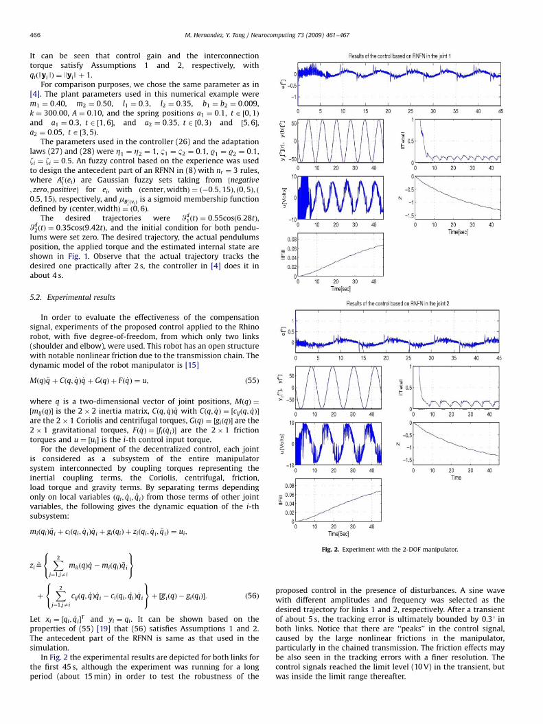
Fig. 2. Experiment with the 2-DOF manipulator.

M. Hernandez, Y. Tang / Neurocomputing 73 (2009) 461–467466

It can be seen that control gain and the interconnectiontorque satisfy Assumptions 1 and 2, respectively, withqiðJyiJÞ ¼ JyiJþ 1.

For comparison purposes, we chose the same parameter as in[4]. The plant parameters used in this numerical example werem1 ¼ 0:40, m2 ¼ 0:50, l1 ¼ 0:3, l2 ¼ 0:35, b1 ¼ b2 ¼ 0:009,k ¼ 300:00, A ¼ 0:10, and the spring positions a1 ¼ 0:1; t 2 ½0;1Þand a1 ¼ 0:3; t 2 ½1;6�, and a2 ¼ 0:35; t 2 ½0;3Þ and ½5;6�,a2 ¼ 0:05; t 2 ½3;5Þ.

The parameters used in the controller (26) and the adaptationlaws (27) and (28) were Z1 ¼ Z2 ¼ 1, B1 ¼ B2 ¼ 0:1, R1 ¼ R2 ¼ 0:1,zi ¼ zi ¼ 0:5. An fuzzy control based on the experience was usedto design the antecedent part of an RFNN in (8) with nr ¼ 3 rules,where Ar

i ðeiÞ are Gaussian fuzzy sets taking from fnegative

; zero; positiveg for ei, with ðcenter;widthÞ ¼ ð�0:5;15Þ; ð0;5Þ; ð0:5;15Þ, respectively, and mBr

iðviÞ

is a sigmoid membership functiondefined by ðcenter;widthÞ ¼ ð0;6Þ.

The desired trajectories were Wd1ðtÞ ¼ 0:55cosð6:28tÞ,

Wd2ðtÞ ¼ 0:35cosð9:42tÞ, and the initial condition for both pendu-

lums were set zero. The desired trajectory, the actual pendulumsposition, the applied torque and the estimated internal state areshown in Fig. 1. Observe that the actual trajectory tracks thedesired one practically after 2 s, the controller in [4] does it inabout 4 s.

5.2. Experimental results

In order to evaluate the effectiveness of the compensationsignal, experiments of the proposed control applied to the Rhinorobot, with five degree-of-freedom, from which only two links(shoulder and elbow), were used. This robot has an open structurewith notable nonlinear friction due to the transmission chain. Thedynamic model of the robot manipulator is [15]

MðqÞ €q þ Cðq; _qÞ _q þ GðqÞ þ Fð _qÞ ¼ u; ð55Þ

where q is a two-dimensional vector of joint positions, MðqÞ ¼

½mijðqÞ� is the 2� 2 inertia matrix, Cðq; _qÞ €q with Cðq; _qÞ ¼ ½cijðq; _qÞ�are the 2� 1 Coriolis and centrifugal torques, GðqÞ ¼ ½giðqÞ� are the2� 1 gravitational torques, Fð _qÞ ¼ ½fið _qiÞ� are the 2� 1 frictiontorques and u ¼ ½ui� is the i-th control input torque.

For the development of the decentralized control, each jointis considered as a subsystem of the entire manipulatorsystem interconnected by coupling torques representing theinertial coupling terms, the Coriolis, centrifugal, friction,load torque and gravity terms. By separating terms dependingonly on local variables ðqi; _qi; €qiÞ from those terms of other jointvariables, the following gives the dynamic equation of the i-thsubsystem:

miðqiÞ €qi þ ciðqi; _qiÞ _qi þ giðqiÞ þ ziðqi; _qi; €qiÞ ¼ ui;

zi9X2

j¼1;jai

miiðqÞ _q �miðqiÞ €qi

8<:

9=;

þX2

j¼1;jai

cijðq; _qÞ _qi � ciðqi; _qi Þ _qi

8<:

9=;þ ½giðqÞ � giðqiÞ�: ð56Þ

Let xi ¼ ½qi; _qi�T and yi ¼ qi. It can be shown based on the

properties of (55) [19] that (56) satisfies Assumptions 1 and 2.The antecedent part of the RFNN is same as that used in thesimulation.

In Fig. 2 the experimental results are depicted for both links forthe first 45 s, although the experiment was running for a longperiod (about 15 min) in order to test the robustness of the

proposed control in the presence of disturbances. A sine wavewith different amplitudes and frequency was selected as thedesired trajectory for links 1 and 2, respectively. After a transientof about 5 s, the tracking error is ultimately bounded by 0.31 inboth links. Notice that there are ‘‘peaks’’ in the control signal,caused by the large nonlinear frictions in the manipulator,particularly in the chained transmission. The friction effects maybe also seen in the tracking errors with a finer resolution. Thecontrol signals reached the limit level (10 V) in the transient, butwas inside the limit range thereafter.

ARTICLE IN PRESS

M. Hernandez, Y. Tang / Neurocomputing 73 (2009) 461–467 467

6. Conclusions

This paper has presented the design of an adaptive output-feedback decentralized control for the class of second ordernonlinear affine interconnected systems. By using the proposedrecurrent neural network, no separated state estimate wasneeded. A practical assumption (Assumption 3) was made forestablishing practical stability. Numerical simulation in twocoupled pendulums and experiment validation in a two degree-of-freedom robot arm were carried out for comparison andvalidation purposes.

References

[1] V.H. Benitez, E. N. Sanchez, A.G. Loukianov, Decentralized adaptive recurrentneural control structure, Artif. Intell. 20 (2007) 1125–1132.

[2] D.T. Gavel, D.D. Siljak, Decentralized adaptive control: structural conditionsfor stability, IEEE Trans. Automat. Control 34 (1989) 413–426.

[3] J.J. Hopfield, Neurons with graded response have collective computationproperties like those of two-state neurons, Proc. Natl. Acad. Sci. 81 (1984)3088–3092.

[4] S. Huang, K.K. Tan, T.H. Lee, Decentralized control design for large-scalesystems with strong interconnections using neural networks, IEEE Trans.Automat. Control 48 (2003) 805–810.

[5] P.A. Ioannou, Decentralized adaptive control on interconnected systems, IEEETrans. Automat. Control 34 (1986) 291–298.

[6] C.F. Juang, A TSK-type recurrent fuzzy network for dynamic systemsprocessing by neural network and genetic algorithms, IEEE Trans. Fuzzy Syst.10 (2002) 155–170.

[7] H.K. Khalil, Nonlinear Systems, third ed., Prentice-Hall, Englewood Cliffs, NJ,2002.

[8] R. Kelly, Global positioning on robot manipulators via PD control plus a classof nonlinear integral actions, IEEE Bans. Automat. Control 43 (74) (1998).

[9] A. Levin, K.S. Narendra, Control of nonlinear dynamical systems using neuralnetworks—Part II: observability, identification, and control, IEEE Trans.Neural Networks 7 (1996) 30–42.

[10] G.A. Rovithakis, Adaptive Control with Recurrent High-order Neural Net-works: Theory and Industrial Applications, Springer, Berlin, 2000.

[11] R.M. Sanner, J.J.E. Slotine, Gaussian networks for direct adaptive control, IEEETrans. Neural Networks 3 (1992) 837–863.

[12] H. Seraji, Decentralized adaptive controller of manipulators: theory, simula-tion and experimentation, IEEE Trans. Robotics Autom. 5 (1989) 183–201.

[13] D.D. Siljak, Decentralized Control of Complex Systems, Academic Press, SanDiego, 1991.

[14] L. Shi, S.K. Singh, Decentralized adaptive controller design for large-scalesystems with higher order interconnections, IEEE Trans. Automat. Control 37(1992) 1106–1118.

[15] M. Spong, M. Vidyasagar, Robot Dynamics and Control, Wiley, New York, 1989.[16] J.T. Spooner, K.M. Passino, Decentralized adaptive control of nonlinear

systems using radial basis neural networks, IEEE Trans. Autom. Control 44(1999) 2050–2057.

[17] T. Takagi, M. Sugeno, Fuzzy identification of systems and its applications tomodeling and control, IEEE Trans. Syst. Man Cybern. SMC-15 (1984) 116–132.

[18] P. Tomei, Adaptive PD controller for robot manipulator, IEEE Bans. Autom.Control 36 (1992) 556–570.

[19] Y. Tang, M. Tomizuka, G. Guerrero-Ramırez, G. Montemayo, Decentralizedrobust control of mechanical systems, IEEE Trans. Autom. Control 45 (2000)771–776.

[20] S. Tong, H.X. Li, G. Chen, Adaptive fuzzy decentralized control for a class oflarge-scale nonlinear systems, IEEE Trans. Syst. Man Cybern. Part B Cybern. 34(2004) 770–775.

[21] D. V�elez, Y. Tang, Adaptive robust fuzzy control of uncertain nonlinearsystems, IEEE Trans. Man Syst. Cybern. B 11 (2003) 401–409.

[22] L. Wang, Adaptive Fuzzy Systems and Control, Design and Stability Analysis,Prentice-Hall, Englewood Cliffs, NJ, 1994.

Miguel Hern �andez He obtained the Doctor’s degree(2008), the Master’s degree (2004) and the Bachelor’sdegree (2003), all in Electrical Engineering from theNational University of Mexico. He is now with theUniversity of ISTHMUS as a researcher-professor,working on projects related with power systems andprocess control.

Yu Tang After getting his Ph.D. degree in electrical engineering from the NationalUniversity of Mexico in 1988, he joined the same university and is currently a FullProfessor at the Faculty of Engineering. He was a Guest Professor at the BeijingUniversity of Technology in 1997–2001. He hold a research position with theUniversity of California, Berkeley in 1996, Mexican Petroleum Institute in 2002,and was a Consultant for the Mexican Institute of Research in Electricity in 1994–1995. His research interests include adaptive control, intelligent control, androbotics, and their applications to industrial problems.

Dr. Tang is a Regular Member of the Mexican Academy of Sciences and System ofNational Investigators (SNI). He received the Weizmann Prize from the MexicanAcademy of Sciences for the Best Ph.D. Dissertation in 1991, the ‘‘NationalUniversity Distinction for Young Academics’’ in 1995, and the ‘‘National UniversityRecognized Professor’’ in 1997, both from the National University of Mexico.