adaptive regularization of weight...
TRANSCRIPT

Adaptive Regularization of Weight Vectors
Koby CrammerDepartment of
Electrical EngineringThe Technion
Haifa, 32000 [email protected]
Alex KuleszaDepartment of Computerand Information Science
University of PennsylvaniaPhiladelphia, PA [email protected]
Mark DredzeHuman Language Tech.
Center of ExcellenceJohns Hopkins University
Baltimore, MD [email protected]
Abstract
We present AROW, a new online learning algorithm that combines sev-eral useful properties: large margin training, confidence weighting, and thecapacity to handle non-separable data. AROW performs adaptive regular-ization of the prediction function upon seeing each new instance, allowingit to perform especially well in the presence of label noise. We derivea mistake bound, similar in form to the second order perceptron bound,that does not assume separability. We also relate our algorithm to recentconfidence-weighted online learning techniques and show empirically thatAROW achieves state-of-the-art performance and notable robustness in thecase of non-separable data.
1 Introduction
Online learning algorithms are fast, simple, make few statistical assumptions, and performwell in a wide variety of settings. Recent work has shown that parameter confidence in-formation can be effectively used to guide online learning [2]. Confidence weighted (CW)learning, for example, maintains a Gaussian distribution over linear classifier hypothesesand uses it to control the direction and scale of parameter updates [6]. In addition to for-mal guarantees in the mistake-bound model [11], CW learning has achieved state-of-the-artperformance on many tasks. However, the strict update criterion used by CW learning isvery aggressive and can over-fit [5]. Approximate solutions can be used to regularize theupdate and improve results; however, current analyses of CW learning still assume that thedata are separable. It is not immediately clear how to relax this assumption.
In this paper we present a new online learning algorithm for binary classification that com-bines several attractive properties: large margin training, confidence weighting, and thecapacity to handle non-separable data. The key to our approach is the adaptive regular-ization of the prediction function upon seeing each new instance, so we call this algorithmAdaptive Regularization of Weights (AROW). Because it adjusts its regularization for eachexample, AROW is robust to sudden changes in the classification function due to labelnoise. We derive a mistake bound, similar in form to the second order perceptron bound,that does not assume separability. We also provide empirical results demonstrating thatAROW is competitive with state-of-the-art methods and improves upon them significantlyin the presence of label noise.
2 Confidence Weighted Online Learning of Linear Classifiers
Online algorithms operate in rounds. In round t the algorithm receives an instance xt ∈ Rd
and applies its current prediction rule to make a prediction yt ∈ Y. It then receives the true
1

label yt ∈ Y and suffers a loss `(yt, yt). For binary classification we have Y = {−1,+1} anduse the zero-one loss `01(yt, yt) = 0 if yt = yt and 1 otherwise. Finally, the algorithm updatesits prediction rule using (xt, yt) and proceeds to the next round. In this work we considerlinear prediction rules parameterized by a weight vector w: y = hw(x) = sign(w · x).
Recently Dredze, Crammer and Pereira [6, 5] proposed an algorithmic framework for on-line learning of binary classification tasks called confidence weighted (CW) learning. CWlearning captures the notion of confidence in a linear classifier by maintaining a Gaussiandistribution over the weights with mean µ ∈ Rd and covariance matrix Σ ∈ Rd×d. Thevalues µp and Σp,p, respectively, encode the learner’s knowledge of and confidence in theweight for feature p: the smaller Σp,p, the more confidence the learner has in the meanweight value µp. Covariance terms Σp,q capture interactions between weights.
Conceptually, to classify an instance x, a CW classifier draws a parameter vector w ∼N (µ,Σ) and predicts the label according to sign(w · x). In practice, however, it can beeasier to simply use the average weight vector E [w] = µ to make predictions. This is similarto the approach taken by Bayes point machines [9], where a single weight vector is used toapproximate a distribution. Furthermore, for binary classification, the prediction given bythe mean weight vector turns out to be Bayes optimal.
CW classifiers are trained according to a passive-aggressive rule [3] that adjusts the dis-tribution at each round to ensure that the probability of a correct prediction is at leastη ∈ (0.5, 1]. This yields the update constraint Pr [yt (w · xt) ≥ 0] ≥ η . Subject to thisconstraint, the algorithm makes the smallest possible change to the hypothesis weight dis-tribution as measured using the KL divergence. This implies the following optimizationproblem for each round t:
(µt,Σt) = minµ,Σ
DKL
(N (µ,Σ) ‖N
(µt−1,Σt−1
))s.t. Prw∼N (µ,Σ) [yt (w · xt) ≥ 0] ≥ η
Confidence-weighted algorithms have been shown to perform well in practice [5, 6], but theysuffer from several problems. First, the update is quite aggressive, forcing the probabilityof predicting each example correctly to be at least η > 1/2 regardless of the cost to theobjective. This may cause severe over-fitting when labels are noisy; indeed, current analysesof the CW algorithm [5] assume that the data are linearly separable. Second, they aredesigned for classification, and it is not clear how to extend them to alternative settingssuch as regression. This is in part because the constraint is written in discrete terms wherethe prediction is either correct or not.
We deal with both of these issues, coping more effectively with label noise and generalizingthe advantages of CW learning in an extensible way.
3 Adaptive Regularization Of Weights
We identify two important properties of the CW update rule that contribute to its goodperformance but also make it sensitive to label noise. First, the mean parameters µ areguaranteed to correctly classify the current training example with margin following eachupdate. This is because the probability constraint Pr [yt (w · xt) ≥ 0] ≥ η can be writtenexplicitly as yt (µ · xt) ≥ φ
√x>t Σxt, where φ > 0 is a positive constant related to η.
This aggressiveness yields rapid learning, but given an incorrectly labeled example, it canalso force the learner to make a drastic and incorrect change to its parameters. Second,confidence, as measured by the inverse eigenvalues of Σ, increases monotonically with everyupdate. While it is intuitive that our confidence should grow as we see more data, thisalso means that even incorrectly labeled examples causing wild parameter swings result inartificially increased confidence.
In order to maintain the positives but reduce the negatives of these two properties, weisolate and soften them. As in CW learning, we maintain a Gaussian distribution overweight vectors with mean µ and covariance Σ; however, we recast the above characteristicsof the CW constraint as regularizers, minimizing the following unconstrained objective on
2

each round:
C (µ,Σ) = DKL
(N (µ,Σ) ‖N
(µt−1,Σt−1
))+ λ1`h2 (yt,µ · xt) + λ2x
>t Σxt , (1)
where `h2 (yt,µ · xt) = (max{0, 1− yt(µ · xt)})2 is the squared-hinge loss suffered using theweight vector µ to predict the output for input xt when the true output is yt. λ1, λ2 ≥ 0 aretwo tradeoff hyperparameters. For simplicity and compactness of notation, in the followingwe will assume that λ1 = λ2 = 1/(2r) for some r > 0.
The objective balances three desires. First, the parameters should not change radically oneach round, since the current parameters contain information about previous examples (firstterm). Second, the new mean parameters should predict the current example with low loss(second term). Finally, as we see more examples, our confidence in the parameters shouldgenerally grow (third term).
Note that this objective is not simply the dualization of the CW constraint, but a newformulation inspired by the properties discussed above. Since the loss term depends on µonly via the inner-product µ ·xt, we are able to prove a representer theorem (Sec. 4). Whilewe use the squared-hinge loss for classification, different loss functions, as long as they areconvex and differentiable in µ, yield algorithms for different settings.1
To solve the optimization in (1), we begin by writing the KL explicitly:
C (µ,Σ) =12
log(
det Σt−1
det Σ
)+
12Tr(Σ−1
t−1Σ)
+12(µt−1 − µ
)>Σ−1t−1
(µt−1 − µ
)− d
2
+12r
`h2 (yt,µ · xt) +12r
x>t Σxt (2)
We can decompose the result into two terms: C1(µ), depending only on µ, and C2(Σ), de-pending only on Σ. The updates to µ and Σ can therefore be performed independently.The squared-hinge loss yields a conservative (or passive) update for µ in which the meanparameters change only when the margin is too small, and we follow CW learning by en-forcing a correspondingly conservative update for the confidence parameter Σ, updating itonly when µ changes. This results in fewer updates and is easier to analyze. Our updatethus proceeds in two stages.
1. Update the mean parameters: µt = arg minµC1 (µ) (3)
2. If µt 6= µt−1, update the confidence parameters: Σt = arg minΣC2 (Σ) (4)
We now develop the update equations for (3) and (4) explicitly, starting with the former.Taking the derivative of C (µ,Σ) with respect to µ and setting it to zero, we get
µt = µt−1 −12r
[d
dz`h2 (yt, z) |z=µt·xt
]Σt−1xt , (5)
assuming Σt−1 is non-singular. Substituting the derivative of the squared-hinge loss in (5)and assuming 1− yt (µt · xt) ≥ 0, we get
µt = µt−1 +yt
r(1− yt (µt · xt))Σt−1xt . (6)
We solve for µt by taking the dot product of each side of the equality with xt and substitutingback in (6) to obtain the rule
µt = µt−1 +max
(0, 1− ytx
>t µt−1
)x>t Σt−1xt + r
Σt−1ytxt . (7)
It can be easily verified that (7) satisfies our assumption that 1− yt (µt · xt) ≥ 0.
1It can be shown that the well known recursive least squares (RLS) regression algorithm [7] is aspecial case of AROW with the squared loss.
3
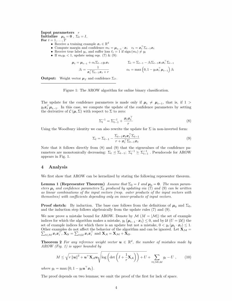
Input parameters rInitialize µ0 = 0 , Σ0 = I,For t = 1, . . . , T
• Receive a training example xt ∈ Rd
• Compute margin and confidence mt = µt−1 · xt vt = x>t Σt−1xt
• Receive true label yt, and suffer loss `t = 1 if sign (mt) 6= yt
• If mtyt < 1, update using eqs. (7) & (9):
µt = µt−1 + αtΣt−1ytxt Σt = Σt−1 − βtΣt−1xtx>t Σt−1
βt =1
x>t Σt−1xt + rαt = max
“0, 1 − ytx
>t µt−1
”βt
Output: Weight vector µT and confidence ΣT .
Figure 1: The AROW algorithm for online binary classification.
The update for the confidence parameters is made only if µt 6= µt−1, that is, if 1 >
ytx>t µt−1. In this case, we compute the update of the confidence parameters by setting
the derivative of C (µ,Σ) with respect to Σ to zero:
Σ−1t = Σ−1
t−1 +xtx
>t
r(8)
Using the Woodbury identity we can also rewrite the update for Σ in non-inverted form:
Σt = Σt−1 −Σt−1xtx
>t Σt−1
r + x>t Σt−1xt(9)
Note that it follows directly from (8) and (9) that the eigenvalues of the confidence pa-rameters are monotonically decreasing: Σt � Σt−1; Σ−1
t � Σ−1t−1 . Pseudocode for AROW
appears in Fig. 1.
4 Analysis
We first show that AROW can be kernelized by stating the following representer theorem.
Lemma 1 (Representer Theorem) Assume that Σ0 = I and µ0 = 0. The mean param-eters µt and confidence parameters Σt produced by updating via (7) and (9) can be writtenas linear combinations of the input vectors (resp. outer products of the input vectors withthemselves) with coefficients depending only on inner-products of input vectors.
Proof sketch: By induction. The base case follows from the definitions of µ0 and Σ0,and the induction step follows algebraically from the update rules (7) and (9).
We now prove a mistake bound for AROW. Denote by M (M = |M|) the set of exampleindices for which the algorithm makes a mistake, yt
(µt−1 · xt
)≤ 0, and by U (U = |U|) the
set of example indices for which there is an update but not a mistake, 0 < yt (µt · xt) ≤ 1.Other examples do not affect the behavior of the algorithm and can be ignored. Let XM =∑
t∈M xix>i , XU =
∑t∈U xix
>i and XA = XM + XU .
Theorem 2 For any reference weight vector u ∈ Rd, the number of mistakes made byAROW (Fig. 1) is upper bounded by
M ≤√
r ‖u‖2 + u>XAu
√log(
det(
I +1rXA
))+ U +
∑t∈M∪U
gt − U , (10)
where gt = max(0, 1− ytu
>xt
).
The proof depends on two lemmas; we omit the proof of the first for lack of space.
4

Lemma 3 Let `t = max(0, 1− ytµ
>t−1xt
)and χt = x>t Σt−1xt. Then, for every t ∈M∪U ,
u>Σ−1t µt = u>Σ−1
t−1µt−1 +ytu
>xt
r
µ>t Σ−1t µt = µ>t−1Σ
−1t−1µt−1 +
χt + r − `2t r
r (χt + r)
Lemma 4 Let T be the number of rounds. Then∑t
χtr
r (χt + r)≤ log
(det(Σ−1
T+1
)).
Proof: We compute the following quantity:
x>t Σtx>t = x>t
(Σt−1 − βtΣt−1xtx
>t Σt−1
)xt = χt −
χ2t
χt + r=
χtr
χt + r.
Using Lemma D.1 from [2] we have that
1rx>t Σtx
>t = 1−
det(Σ−1
t−1
)det(Σ−1
t
) . (11)
Combining, we get∑t
χtr
r (χt + r)=∑
t
(1−
det(Σ−1
t−1
)det(Σ−1
t
) ) ≤ −∑
t
log
(det(Σ−1
t−1
)det(Σ−1
t
) ) ≤ log(det(Σ−1
T+1
)).
We now prove Theorem 2.
Proof: We iterate the first equality of Lemma 3 to get
u>Σ−1T µT =
∑t∈M∪U
ytu>xt
r≥
∑t∈M∪U
1− gt
r=
M + U
r− 1
r
∑t∈M∪U
gt . (12)
We iterate the second equality to get
µ>T Σ−1T µT =
∑t∈M∪U
χt + r − `2t r
r (χt + r)=
∑t∈M∪U
χt
r (χt + r)+
∑t∈M∪U
1− `2tχt + r
. (13)
Using Lemma 4 we have that the first term of (13) is upper bounded by 1r log
(det(Σ−1
T
)).
For the second term in (13) we consider two cases. First, if a mistake occurred on examplet, then we have that yt
(xt · µt−1
)≤ 0 and `t ≥ 1, so 1− `2t ≤ 0. Second, if an the algorithm
made an update (but no mistake) on example t, then 0 < yt
(xt · µt−1
)≤ 1 and `t ≥ 0,
thus 1− `2t ≤ 1. We therefore have∑t∈M∪U
1− `2tχt + r
≤∑t∈M
0χt + r
+∑t∈U
1χt + r
=∑t∈U
1χt + r
. (14)
Combining and plugging into the Cauchy-Schwarz inequality
u>Σ−1T µT ≤
√u>Σ−1
T u√
µ>T Σ−1T µT ,
we get
M + U
r− 1
r
∑t∈M∪U
gt ≤√
u>Σ−1T u
√1r
log(det(Σ−1
T
))+∑t∈U
1χt + r
. (15)
Rearranging the terms and using the fact that χt ≥ 0 yields
M ≤√
r√
u>Σ−1T u
√log(det(Σ−1
T
))+ U +
∑t∈M∪U
gt − U .
5

By definition,
Σ−1T =I +
1r
∑t∈M∪U
xix>i =I +
1rXA ,
so substituting and simplifying completes the proof:
M ≤√
r
√u>(
I +1rXA
)u
√log(
det(
I +1rXA
))+ U +
∑t∈M∪U
gt − U
=√
r ‖u‖2 + u>XAu
√log(
det(
I +1rXA
))+ U +
∑t∈M∪U
gt − U .
A few comments are in order. First, the two square-root terms of the bound depend on rin opposite ways: the first is monotonically increasing, while the second is monotonicallydecreasing. One could expect to optimize the bound by minimizing over r. However, thebound also depends on r indirectly via other quantities (e.g. XA), so there is no direct wayto do so. Second, if all the updates are associated with errors, that is, U = ∅, then the boundreduces to the bound of the second-order perceptron [2]. In general, however, the boundsare not comparable since each depends on the actual runtime behavior of its algorithm.
5 Empirical Evaluation
We evaluate AROW on both synthetic and real data, including several popular datasetsfor document classification and optical character recognition (OCR). We compare withthree baselines: Passive-Aggressive (PA), Second Order Perceptron (SOP)2 and Confidence-Weighted (CW) learning3.
Our synthetic data are as in [5], but we invert the labels on 10% of the training examples.(Note that evaluation is still done against the true labels.) Fig. 2(a) shows the online learningcurves for both full and diagonalized versions of the algorithms on these noisy data. AROWimproves over all competitors, and the full version outperforms the diagonal version. Notethat CW-full performs worse than CW-diagonal, as has been observed previously for noisydata.
We selected a variety of document classification datasets popular in the NLP community,summarized as follows. Amazon: Product reviews to be classified into domains (e.g.,books or music) [6]. We created binary datasets by taking all pairs of the six domains (15datasets). Feature extraction follows [1] (bigram counts). 20 Newsgroups: Approximately20,000 newsgroup messages partitioned across 20 different newsgroups4. We binarized thecorpus following [6] and used binary bag-of-words features (3 datasets). Each dataset hasbetween 1850 and 1971 instances. Reuters (RCV1-v2/LYRL2004): Over 800,000 man-ually categorized newswire stories. We created binary classification tasks using pairs oflabels following [6] (3 datasets). Details on document preparation and feature extractionare given by [10]. Sentiment: Product reviews to be classified as positive or negative. Weused each Amazon product review domain as a sentiment classification task (6 datasets).Spam: We selected three task A users from the ECML/PKDD Challenge5, using bag-of-words to classify each email as spam or ham (3 datasets). For OCR data we binarized twowell known digit recognition datasets, MNIST6 and USPS, into 45 all-pairs problems. Wealso created ten one vs. all datasets from the MNIST data (100 datasets total).
Each result for the text datasets was averaged over 10-fold cross-validation. The OCRexperiments used the standard split into training and test sets. Hyperparameters (including
2For the real world (high dimensional) datasets, we must drop cross-feature confidence terms by projecting
onto the set of diagonal matrices, following the approach of [6]. While this may reduce performance, we make thesame approximation for all evaluated algorithms.
3We use the “variance” version developed in [6].
4http://people.csail.mit.edu/jrennie/20Newsgroups/
5http://ecmlpkdd2006.org/challenge.html
6http://yann.lecun.com/exdb/mnist/index.html
6

500 1000 1500 2000 2500 3000 3500 4000 4500 5000
200
400
600
800
1000
1200
1400
1600
Instances
Mis
take
s
PerceptronPASOPAROW−fullAROW−diagCW−fullCW−diag
(a) synthetic data
0 2000 4000 6000 8000 10000
Instances0
100
200
300
400
500
600
700
800
Mis
take
s
PACWAROWSOP
0 2000 4000 6000 8000 10000
Instances0
500
1000
1500
2000
Mis
take
s
PACWAROWSOP
(b) MNIST data
Figure 2: Learning curves for AROW (full/diagonal) and baseline methods. (a) 5k synthetictraining examples and 10k test examples (10% noise, 100 runs). (b) MNIST 3 vs. 5 binaryclassification task for different amounts of label noise (left: 0 noise, right: 10%).
r for AROW) and the number of online iterations (up to 10) were optimized using a singlerandomized run. We used 2000 instances from each dataset unless otherwise noted above.In order to observe each algorithm’s ability to handle non-separable data, we performed eachexperiment using various levels of artifical label noise, generated by independently flippingeach binary label with fixed probability.
5.1 Results and Discussion
Noise levelAlgorithm 0.0 0.05 0.1 0.15 0.2 0.3AROW 1.51 1.44 1.38 1.42 1.25 1.25CW 1.63 1.87 1.95 2.08 2.42 2.76PA 2.95 2.83 2.78 2.61 2.33 2.08SOP 3.91 3.87 3.89 3.89 4.00 3.91
Table 1: Mean rank (out of 4, over all datasets) at differ-ent noise levels. A rank of 1 indicates that an algorithmoutperformed all the others.
Our experimental resultsare summarized in Table 1.AROW outperforms the base-lines at all noise levels, butdoes especially well as noiseincreases. More detailedresults for AROW and CW,the overall best performingbaseline, are compared inFig. 3. AROW and CW arecomparable when there is noadded noise, with AROWwinning the majority of the time. As label noise increases (moving across the rows inFig. 3) AROW holds up remarkably well. In almost every high noise evaluation, AROWimproves over CW (as well as the other baselines, not shown). Fig. 2(b) shows the totalnumber of mistakes (w.r.t. noise-free labels) made by each algorithm during training on theMNIST dataset for 0% and 10% noise. Though absolute performance suffers with noise,the gap between AROW and the baselines increases.
To help interpret the results, we classify the algorithms evaluated here according to fourcharacteristics: the use of large margin updates, confidence weighting, a design that acco-modates non-separable data, and adaptive per-instance margin (Table 2). While all of theseproperties can be desirable in different situations, we would like to understand how theyinteract and achieve high performance while avoiding sensitivity to noise.
Large Conf- Non- AdaptiveAlgorithm Margin idence Separable MarginPA Yes No Yes NoSOP No Yes Yes NoCW Yes Yes No YesAROW Yes Yes Yes No
Table 2: Online algorithm properties overview.
Based on the results in Ta-ble 1, it is clear that the com-bination of confidence informa-tion and large margin learningis powerful when label noise islow. CW easily outperformsthe other baselines in such situ-ations, as it has been shown todo in previous work. However,as noise increases, the separa-bility assumption inherent in CW appears to reduce its performance considerably.
7

0.75 0.80 0.85 0.90 0.95 1.00
CW0.75
0.80
0.85
0.90
0.95
1.00
AR
OW
20newsamazonreuterssentimentspam
0.5 0.6 0.7 0.8 0.9 1.0
CW0.5
0.6
0.7
0.8
0.9
1.0
AR
OW
20newsamazonreuterssentimentspam
0.5 0.6 0.7 0.8 0.9 1.0
CW0.5
0.6
0.7
0.8
0.9
1.0
AR
OW
20newsamazonreuterssentimentspam
0.90 0.92 0.94 0.96 0.98 1.00
CW0.90
0.92
0.94
0.96
0.98
1.00
AR
OW
USPS 1 vs. AllUSPS All PairsMNIST 1 vs. All
0.5 0.6 0.7 0.8 0.9 1.0
CW0.5
0.6
0.7
0.8
0.9
1.0
AR
OW
USPS 1 vs. AllUSPS All PairsMNIST 1 vs. All
0.5 0.6 0.7 0.8 0.9 1.0
CW0.5
0.6
0.7
0.8
0.9
1.0
AR
OW
USPS 1 vs. AllUSPS All PairsMNIST 1 vs. All
Figure 3: Accuracy on text (top) and OCR (bottom) binary classification. Plots compareperformance between AROW and CW, the best performing baseline (Table 1). Markersabove the line indicate superior AROW performance and below the line superior CW per-formance. Label noise increases from left to right: 0%, 10% and 30%. AROW improvesrelative to CW as noise increases.
AROW, by combining the large margin and confidence weighting of CW with a soft updaterule that accomodates non-separable data, matches CW’s performance in general whileavoiding degradation under noise. AROW lacks the adaptive margin of CW, suggestingthat this characteristic is not crucial to achieving strong performance. However, we leaveopen for future work the possibility that an algorithm with all four properties might haveunique advantages.
6 Related and Future Work
AROW is most similar to the second order perceptron [2]. The SOP performs the same typeof update as AROW, but only when it makes an error. AROW, on the other hand, updateseven when its prediction is correct if there is insufficient margin. Confidence weighted (CW)[6, 5] algorithms, by which AROW was inspired, update the mean and confidence parameterssimultaneously, while AROW makes a decoupled update and softens the hard constraint ofCW. The AROW algorithm can be seen as a variant of the PA-II algorithm from [3] wherethe regularization is modified according to the data.
Hazan [8] describes a framework for gradient descent algorithms with logarithmic regret inwhich a quantity similar to Σt plays an important role. Our algorithm differs in severalways. First, Hazan [8] considers gradient algorithms, while we derive and analyze algo-rithms that directly solve an optimization problem. Second, we bound the loss directly, notthe cumulative sum of regularization and loss. Third, the gradient algorithms perform aprojection after making an update (not before) since the norm of the weight vector is keptbounded.
Ongoing work includes the development and analysis of AROW style algorithms for othersettings, including a multi-class version following the recent extension of CW to multi-classproblems [4]. Our mistake bound can be extended to this case. Applying the ideas behindAROW to regression problems turns out to yield the well known recursive least squares(RLS) algorithm, for which AROW offers new bounds (omitted). Finally, while we used theconfidence term x>t Σxt in (1), we can replace this term with any differentiable, monotoni-cally increasing function f(x>t Σxt). This generalization may yield additional algorithms.
8

References
[1] John Blitzer, Mark Dredze, and Fernando Pereira. Biographies, bollywood, boom-boxesand blenders: Domain adaptation for sentiment classification. In ACL, 2007.
[2] Nicolo Cesa-Bianchi, Alex Conconi, and Claudio Gentile. A second-order perceptronalgorithm. Siam J. of Comm., 34, 2005.
[3] Koby Crammer, Ofer Dekel, Joseph Keshet, Shai Shalev-Shwartz, and Yoram Singer.Online passive-aggressive algorithms. Journal of Machine Learning Research, 7:551–585, 2006.
[4] Koby Crammer, Mark Dredze, and Alex Kulesza. Multi-class confidence weightedalgorithms. In Empirical Methods in Natural Language Processing (EMNLP), 2009.
[5] Koby Crammer, Mark Dredze, and Fernando Pereira. Exact convex confidence-weightedlearning. In Neural Information Processing Systems (NIPS), 2008.
[6] Mark Dredze, Koby Crammer, and Fernando Pereira. Confidence-weighted linear clas-sification. In International Conference on Machine Learning, 2008.
[7] Simon Haykin. Adaptive Filter Theory. 1996.[8] Elad Hazan. Efficient algorithms for online convex optimization and their applications.
PhD thesis, Princeton University, 2006.[9] Ralf Herbrich, Thore Graepel, and Colin Campbell. Bayes point machines. Journal of
Machine Learning Research (JMLR), 1:245–279, 2001.[10] David D. Lewis, Yiming Yang, Tony G. Rose, and Fan Li. Rcv1: A new benchmark
collection for text categorization research. JMLR, 5:361–397, 2004.[11] Nick Littlestone. Learning when irrelevant attributes abound: A new linear-threshold
algorithm. Machine Learning, 2:285–318, 1988.
9