adaptive remeshing method via inversion of element ... · adaptive remeshing method via inversion...

2010 SIMULIA Customer Conference 1

Adaptive Remeshing Method via Inversion of Element Anisotropy in Large Deformation Finite

Element Analysis Dheeravongkit, A.

King Mongkut's University of Technology Thonburi, Institute of Field Robotics

Abstract: The large deformation finite element analysis such as metal forming analysis usually involves processes to deform, stamp, or punch a part drastically, which causes great changes in shape of the part during the simulation. As the part is reshaped, the mesh elements are deformed, and element shape quality is decaying as analysis continues. To resolve this problem, it is common to adaptively remesh the part during the analysis to replace the unusable mesh with a new better quality mesh. The proposed method is an alternative adaptive remeshing method, which not only locally refines the mesh around the areas that are likely to experience large deformation, but also adjusts the mesh directionality and anisotropy to reduce the severity of element distortion as analysis continues. With this method, the element sizes are adjusted based on the strain rate values at the current stage. The smaller element sizes are specified around the areas with larger strain rate values. For mesh directionality, the element orientations are adjusted to align with the boundary of the part, which helps reducing the chance of severe element distortion. For mesh anisotropy, the proposed method utilizes the change in lengths of each element in the principal directions from the previous steps as the prediction of the future deformation of that element. Then, the method specifies the anisotropy of the newly generated mesh in the opposite manner. For example, if the prediction indicates the ratio of the element’s length in first and second principal directions as 1:2, the method will specify the length ratio of the newly generated element as 2:1. This tactic keeps mesh quality within an acceptable range for a longer period of time than a traditional mesh that starts with an optimal quality and rapidly degrades to an unacceptable quality level as analysis continues. Consequently, the proposed method can help reduce the number of adaptive remeshing required throughout the course of the analysis.

Keywords: Inverse Adaptation, Adaptive Mesh, Adaptive Remeshing, Large Deformation, Metal Forming, Finite Element Analysis.

1. Introduction

Finite Element Method is a very powerful tool to simulate processes on computer in many applications in order to design, analyze, and manufacture parts. This research focuses on the applications involving large deformation processes such as metal forming processes, where the part is greatly deformed into a different shape from the starting shape. Since the mesh representing the workpiece is often deformed severely as analysis continues in this type of process, it leads to computational error caused by the element distortion. These distorted elements are unwanted in finite element analysis, because they introduce errors in computation, as well as geometric

2 2010 SIMULIA Customer Conference

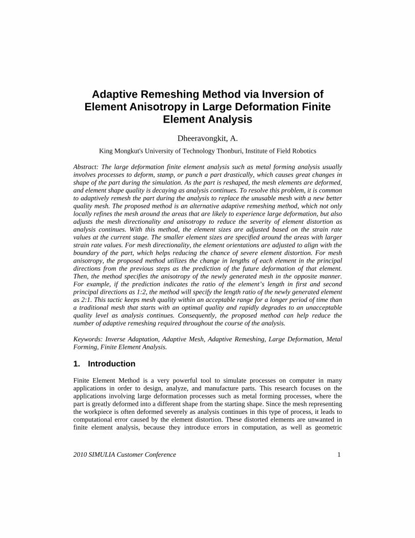
interference error between workpiece and tool. When mesh elements are severely distorted, the analysis is often terminated prematurely, and not able to complete the analysis to the end. One common solution to this problem is to iteratively perform adaptive remeshing during the analysis. The adaptive remeshing [1-11] is a method to repeatedly regenerate a new mesh with optimal element shape quality every time during the simulation that the mesh becomes extremely distorted. Typically, the criteria that are used to determine the time to remesh are mesh discritization error measured by L2 norm of the strain error [2-9], element distortion error measured by element shape quality [3, 4, 10, 11], and geometric interference error measured by interference depth between workpiece and tool [3]. Whenever the error tolerance is exceeded, the existing mesh will be replaced with a new mesh, which generally consists of elements with optimal shape quality, and is locally refined in the area with high error values. Then the solutions are mapped from the old mesh to the newly generated mesh using interpolation function in order to continue the analysis [9]. Normally, the remeshing and solution mapping processes will be repeated several times over the course of the analysis. Consequently, the more iterations of adaptive remeshing are required, the more computational time it will cost. Moreover, performing adaptive remeshing frequently may induce significant loss of accuracy during the state variables mapping process, due to the interpolation approximation. For this reason, any methods developed to help reduce the repetition of the complete remeshing during the simulation would be useful and would bring to more accurate analysis result. Inverse adaptation method is another method developed to help solving the element distortion problem during the analysis [12, 13]. The key concept of this method is to predict the final shapes of the elements after deformation, then generate a new starting mesh, which contains elements with shapes opposite to those predicted. The concept of this method is shown in Figure 1.

Conventional Analysis

1 element

Element with optimal shape Inverted element

• Analysis is terminated prematurely

• Result inaccuracy

Inversely Adapted Element

Shape quality improved Shape quality starts to degrade

Inverse Mesh Adaptation

• Reduce number of inverted elements

• Extend analysis life

Inverse Shape

Figure 1. Key concept of the inverse adaptation method.


It is evident from the previous studies that the mesh generated using this method can successfully delay the occurrence of severely distorted elements and extend the analysis life to the further step before the mesh becomes unusable that needs to be replaced with a new mesh [12, 13]. The method consists of four main steps:

1. Pre-analysis: To predict the element deformation behavior. The analysis will be carried out until the step before the occurrence of any inverted element.

2. Bubble Mesh Generation: To create a new mesh on the domain of deformed part using Bubble Mesh Generator [14, 15]. This new mesh is the ideal mesh we wish to achieve at the current analysis step, in which the element size and orientation are also appropriately controlled.

3. Inverse node mapping: To map the location of the nodes of the new mesh generated by Bubble Mesh Generator back on to the domain of the undeformed part. The result of this step is the inversely adapted mesh.

4. Full analysis: Run the full analysis on the inversely adapted mesh. However, it should be noted that this method only creates the starting mesh or the initial mesh. In other words, it is a method to adapt the initial mesh so that it has appropriate element size, element shape, and element orientation for the particular analysis, not a method that repeatedly generates new meshes over the course of the analysis. This leads to the motivation of this research to apply the inverse adaptation concept as an alternative way to generate new mesh during the adaptive remeshing process. Therefore, the main purposes of this research are to develop a method to iteratively adapt mesh utilizing the inverse adaptation concept in order to

• Reduce the severity of element distortion during the analysis • Extend the analysis life before requiring another remeshing • Achieve better result accuracy • Keep the minimum number of nodes and elements

2. Key concept of the proposed method

This section discusses the key concept of the proposed method and the differences between the proposed method, conventional adaptive remeshing method, and the inverse adaptation method. Consider an element in a mesh domain as shown in Figure 2 (a). This element has an optimal shape quality at the initial stage. However, the shape quality is often degrading and eventually becomes severely distorted or inverted as analysis continues. In the conventional adaptive remeshing method, when the element quality becomes unacceptable, it will be replaced with a better quality element as shown in Figure 2 (b). Again, as analysis continues, this shape quality will be degraded and the remeshing process will be repeated. Alternatively, the proposed inversely adaptive remeshing method can be performed as shown in Figure 2 (c). The key concept is to utilize the previous steps of simulation to predict the way the mesh will be deformed in the next steps of the analysis, δ , and then pre-deforms the new mesh in the opposite manner, 1−δ . So the inversely adapted mesh contains elements with shapes


approximately inverse of the shapes they should be deformed into in the general analysis. The clear advantage of this technique is that the inversely adapted mesh is generated so that the mesh elements start out slightly distorted but still in the acceptable quality range, and as analysis continues on this mesh the element shapes will be improved until they reach the optimal quality and begin to degrade again later in the analysis. For this reason, the proposed method can keep the mesh quality within an acceptable range for a longer period of time than with a conventional method, and allows the analysis to run longer before being terminated by poor quality elements. Consequently, it can extend the life of the analysis and potentially reduce or eliminate the need for multiple remeshings during the simulation. Moreover, this approach also incorporates the idea of averaging out the error over the course of the analysis instead of accumulating error rapidly during the simulation.

Figure 2. Key concept of the proposed method.

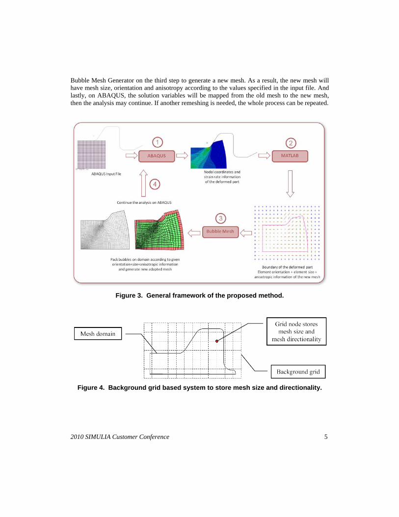
3. General framework

The general framework of the proposed method consists of four main steps as illustrated on Figure 3. On the first step the pre-analysis is performed on a simple uniform mesh. The pre-analysis is carried out until it reaches the analysis step where remeshing is needed. Then on the second step the deformed mesh domain and strain information from the pre-analysis are input to a computer program written on MATLAB to determine the appropriate element size, element orientation and element anisotropy. These pieces of information will be stored on a background grid based system, which is defined to cover the whole mesh domain as shown in Figure 4. The computed values of element size, element orientation and element anisotropy will be stored at the grid nodes. Any value at the internal point inside the grid cell can be obtained by linearly interpolating the values at the cell’s grid nodes. Then this information will be passed on as an input file to the

(a)

(b)

(c)


Bubble Mesh Generator on the third step to generate a new mesh. As a result, the new mesh will have mesh size, orientation and anisotropy according to the values specified in the input file. And lastly, on ABAQUS, the solution variables will be mapped from the old mesh to the new mesh, then the analysis may continue. If another remeshing is needed, the whole process can be repeated.

Figure 3. General framework of the proposed method.

Figure 4. Background grid based system to store mesh size and directionality.


Figure 5 illustrates the data flow of the process. On the first step, the geometric data and strain information of the distorted mesh will be obtained from ABAQUS. On the second step, the program written on MATLAB will first extract element size, orientation and anisotropy. Then invert the anisotropy and make the tensor field input file for the Bubble Mesh Generator. On the third step, the Bubble Mesh Generator receives the input file from the previous step and generates the new mesh. Then, on the last step, the solution is mapped on the new mesh and simulation continues on ABAQUS. The following section will explain each step of the proposed method in detail.

3.1 Pre-analysis

Figure 6. Pre-analysis step.

The goal of this step is to collect the geometric information of the deformed mesh and strain rate values. The geometric information are the nodal coordinates and the element connectivity, which will be used as the domain to generate new mesh on Bubble Mesh Generator in the later step. The strain rate is a scalar variable that represents the rate of material’s deformation. In this research, this information is used to control the element size of the new mesh that we are generating. Finite element discritization error is used as the remesh criteria to determine the step time to perform remeshing. The discritization error can be directly obtained from ABAQUS by including error indicator variable output request.


Figure 5. Data flow of the process of the proposed method.


3.2 Determine Mesh Size, Orientation and Anisotropy

Figure 7. Step to determine mesh size, orientation and anisotropy.

The goal of this step is to determine the appropriate element size, element orientation, and element anisotropy by a program written in MATLAB. The inputs are the geometric information of the deformed mesh and the strain rate obtained from the pre-analysis. The outputs are the tensor field file contains the information of element size, orientation and anisotropy on the background grid nodes, as well as the boundary information of the deformed part. The following subsections explain the method used to determine element size, element orientation and element anisotropy.

3.2.1 Element size

To determine the element size, the strain rate information is used. In short, smaller elements will be specified around the locations with higher strain rate values, where it tends to experience more severe element distortion. To calculate element size, the minimum and maximum element sizes are first specified by the user. Then maximum element size is assumed for minimum strain value and vice versa. Because the change in element size should be more rapid than the change in strain value, so by experiments a decent result can be obtained by utilizing a cubic function to describe the relation between the element sizes and strain values. Equation 1 is the equation of the cubic function. Figure 8 shows the plot of the cubic function.

( )( )

( ) minminmax3maxmin

3max)( llll +

−⋅

−

−=

εεεεε (1)


Figure 8. Cubic function to interpolate the element size.

3.2.2 Element orientation

Element orientation is stored on Bubble Mesh generator as a 3 by 3 tensor at each background grid node. This 3 by 3 tensor represents the three principal vectors at that point. For two-dimensional problems, the third vector is normal to the plane. For this research, the orientations of the elements are specified to align with the boundary of the mesh domain in order to reduce the chance of severe element distortion as shown in Figure 7. To determine the principal vectors, for each grid node, the program searches for the closest boundary edge, then sets the orientation of the closest edge as tangential vector, calculates a normal vector to that edge, and sets it as normal vector.

3.2.3 Element anisotropy

Figure 9. Step to compute element anisotropy.

The element anisotropy is determined by the change of the length ratio of the bounding box created to cover each element in the direction of tangential and normal vector found in the previous section. Equation 2 is used to calculate the ratio of the element’s tangential length and normal length before deformation. Equation 3 is used to calculate the ratio after deformation. And

T-Vec0

N-Vec0

T-L0

N-L0

Before Deformation

T-Vec1 N-Vec1

T-L1 N-L1

After Deformation

N-Vec : Normal Vector T-Vec : Tangential Vector N-L : Element length in normal direction T-L : Element length in tangential direction


Equation 4 is used to determine the ratio that represents how the element lengths change in each direction. The inverse of the calculated ratio will be used to specify the anisotropy of the new mesh so it contains elements with shapes opposite to those predicted.

1:1: 00

0 RLL

N

T = (2)

1:1: 11

1 RLL

N

T = (3)

1:0

1RR

(4)

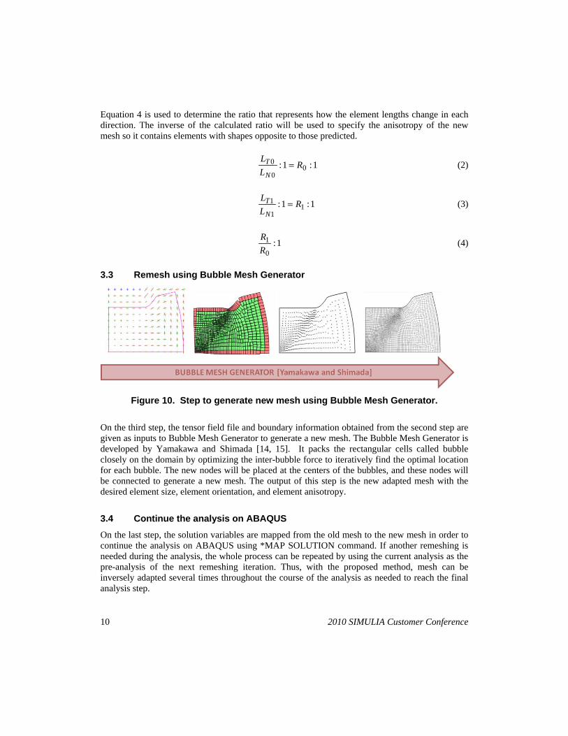
3.3 Remesh using Bubble Mesh Generator

Figure 10. Step to generate new mesh using Bubble Mesh Generator.

On the third step, the tensor field file and boundary information obtained from the second step are given as inputs to Bubble Mesh Generator to generate a new mesh. The Bubble Mesh Generator is developed by Yamakawa and Shimada [14, 15]. It packs the rectangular cells called bubble closely on the domain by optimizing the inter-bubble force to iteratively find the optimal location for each bubble. The new nodes will be placed at the centers of the bubbles, and these nodes will be connected to generate a new mesh. The output of this step is the new adapted mesh with the desired element size, element orientation, and element anisotropy.

3.4 Continue the analysis on ABAQUS On the last step, the solution variables are mapped from the old mesh to the new mesh in order to continue the analysis on ABAQUS using *MAP SOLUTION command. If another remeshing is needed during the analysis, the whole process can be repeated by using the current analysis as the pre-analysis of the next remeshing iteration. Thus, with the proposed method, mesh can be inversely adapted several times throughout the course of the analysis as needed to reach the final analysis step.


4. Experimental results and discussion

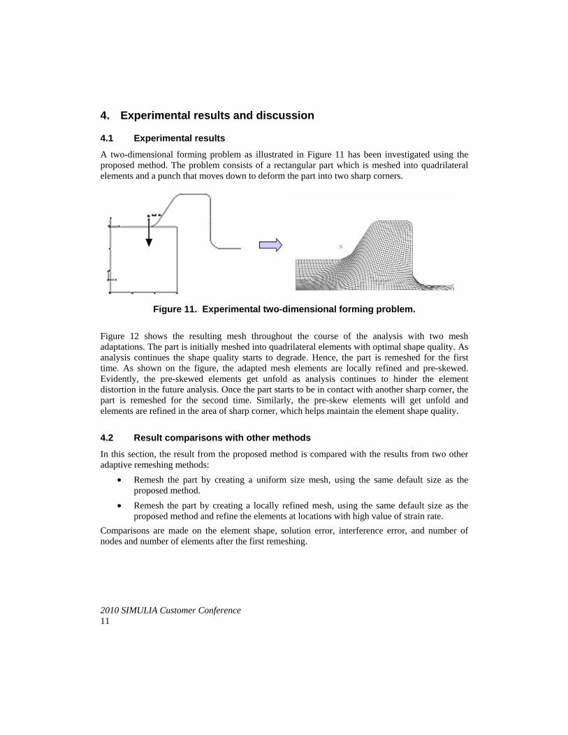
4.1 Experimental results A two-dimensional forming problem as illustrated in Figure 11 has been investigated using the proposed method. The problem consists of a rectangular part which is meshed into quadrilateral elements and a punch that moves down to deform the part into two sharp corners.

Figure 11. Experimental two-dimensional forming problem.

Figure 12 shows the resulting mesh throughout the course of the analysis with two mesh adaptations. The part is initially meshed into quadrilateral elements with optimal shape quality. As analysis continues the shape quality starts to degrade. Hence, the part is remeshed for the first time. As shown on the figure, the adapted mesh elements are locally refined and pre-skewed. Evidently, the pre-skewed elements get unfold as analysis continues to hinder the element distortion in the future analysis. Once the part starts to be in contact with another sharp corner, the part is remeshed for the second time. Similarly, the pre-skew elements will get unfold and elements are refined in the area of sharp corner, which helps maintain the element shape quality.

4.2 Result comparisons with other methods

In this section, the result from the proposed method is compared with the results from two other adaptive remeshing methods:

• Remesh the part by creating a uniform size mesh, using the same default size as the proposed method.

• Remesh the part by creating a locally refined mesh, using the same default size as the proposed method and refine the elements at locations with high value of strain rate.

Comparisons are made on the element shape, solution error, interference error, and number of nodes and number of elements after the first remeshing.


Figure 12. Resulting mesh after performing two adaptive remeshing by the proposed method.

1st Adaptation

2nd Adaptation


4.2.1 Comparing element shape

Figure 13. Comparing element shape quality.

Figure 13 compares the element shape quality of the resulting mesh from the proposed method with resulting mesh from other adaptive remeshing methods applying at the same step of the analysis. According to the results shown in Figure 13, considering the elements around the sharp corners, it is evident that the element shape quality of the proposed method’s mesh has been greatly improved. In contrast, the element shape quality of the uniform size mesh tends to be degrading as elements are being skewed. For the size controlled mesh, the elements around sharp corner are too coarse that they start to interfere with the punch geometry.

Interference between part and tool

Elements being skewed

Proposed Method

Uniform Mesh

Size Controlled


4.2.2 Comparing solution error

Solution errors of the three adaptive remeshing methods are obtained by requesting the error indicator output on ABAQUS. The error is computed based on the patch recovery technique. Figure 14 (a) compares the average plastic strain errors and Figure 14 (b) compares the maximum plastic strain errors throughout the analysis between different adaptive remeshing methods. It is shown on both plots that the solution error of the proposed method has the smallest values among all the methods compared in the beginning phase of the analysis, and performs equally well with the size controlled mesh at the end of the analysis.

(a) (b)

Figure 14. Comparing (a) the average plastic strain error (b) the maximum plastic strain error.

4.2.3 Comparing geometric interference error

Geometric interference error is measured by the interference depth between the part and tool. Table 1 and Figure 15 compare the maximum value of geometric interference depth of the meshes created by the three adaptive remeshing methods at different step times. According to the results, the proposed method can successfully reduce the geometric interference error.

Table 1. Comparing the geometric interference depth at different step times. Step Time Proposed Method Size Controlled Uniform Mesh

0.1 5.54E-06 8.49E-05 3.57E-04 0.2 0 3.85E-05 4.58E-04

0.25 1.28E-04 1.69E-04 4.98E-04 0.3 2.13E-04 1.62E-04 4.29E-04

0.35 3.27E-04 2.51E-04 6.54E-04


Figure 15. Comparing the geometric interference depth at different step times.

4.2.4 Comparing number of nodes and elements

Table 2 gives the total number of nodes and number of elements of the mesh generated by three adaptive remeshing methods.

Table 2. Comparing number of nodes and elements.

Remeshing Method 1st Adaptation 2nd Adaptation # of Nodes # of Elements # of Nodes # of Elements

Mesh of the proposed method 1789 1672 2185 2052 Uniform mesh 1063 994 1527 1447 Mesh with size controlled 1873 1779 2329 2209

5. Conclusion

According to the experimental results, it is evident that the proposed method can successfully adapt mesh during the analysis by generating a new mesh whose elements are pre-deformed inversely to the predicted deformation. From the comparisons of element shape quality, solution error, and geometric interference error between the proposed method and other adaptive remeshing methods, it is clearly shown that the proposed method provides an improved element shape quality. In terms of the solution error and geometric interference, the proposed method and size controlled method appear to perform equally well. Nevertheless, it is shown that the proposed mesh uses less number of nodes and elements comparing to the adapted mesh with size controlled. This is a great advantage of the proposed method. Because the generated mesh is an anisotropic mesh, the elements will be refined only in the particular direction that requires smaller sizes, while keeping normal element sizes in other directions. Therefore, the proposed method can effectively minimize the number of nodes and elements while maximize the efficiency of the mesh.

6. Acknowledgement

This research is funded by Thai Research Fund (TRF). Project number MRG5180229.


7. References

1. Kwak, D.Y. and Im, Y.T., “Remeshing for metal forming simulations PartII: Three-dimensional hexahedral mesh generation,” International Journal for Numerical Methods in Engineering, vol. 53(11), pp. 2501-2528, 2002.

2. Wan, J., Kocak, S., and Shephard, M.S., “Automated Adaptive Forming Simulations,” In Proceedings of 12th Interational Meshing Roundtable, SandiaNational Laboratories, pp. 323-334, 2003.

3. Hattangady, N.V., “Automatic Remeshingin 3-D Analysis of Forming Processes,” International Journal for Numerical Methods in Engineering, 45, pp. 553-568, 1999.

4. Hattangady N.V., “Automated Modeling and Remeshing in Metal Forming Simulation,” Ph.D. thesis, Rensselaer Polytechnic Institute, Troy, NY, 2003.

5. Khoei, A.R. and Lewis, R.W., “Adaptive Finite Element Remeshing in a Large Deformation Analysis of Metal Powder Forming,” International Journal for Numerical Methods in Engineering, vol. 45(7), pp. 801-820, 1999.

6. Merrouche, A., Selman, A., and Knoff-Lenoir, C., “3D Adaptive Mesh Refinement,” Communications in Numerical Methods in Engineering, vol. 14, pp. 397-407, 1998.

7. Zienkiewicz, O.C. and Zhu, J.Z., “The Superconvergent Patch Recovery and A Posteriori Error Estimates. Part1: The Recovery Technique,” International Journal for Numerical Methods in Engineering, vol. 33, pp. 1331-1364, 1992.

8. Zienkiewicz, O.C. and Zhu, J.Z., “The Super-Convergent Patch Recovery and a Posteriori Error Estimates. Part2: Error Estimates and Adaptivity,” International Journal for Numerical Methods in Engineering, vol. 33, pp. 1365-1382, 1992.

9. Meinders, T., “Developments in Numerical Simulations of the Real Life Deep Drawing Process,” Ph.D. thesis, University of Twente, Enschede, The Netherlands, 2000.

10. Joun, M.S. and Lee, M.C., “Quadrilateral Finite-Element Generation and Mesh Quality Control for Metal Forming Simulation,” International Journal for Numerical Methods in Engineering, vol. 40, pp. 4059-4075, 1997.

11. Kwak, D.Y., Cheon, J.S., and Im, Y.T., “Remeshing for Metal Forming Simulations PartI: Two-dimensional Quadrilateral Remeshing,” International Journal for Numerical Methods in Engineering, vol. 53(11), pp. 2463-2500, 2002.

12. Dheeravongkit, A. and Shimada, K., “Inverse Pre-deformation of Finite Element Mesh for Large Deformation Analysis,” In Proceedings of 13th International Meshing Roundtable, Williamsburg, VA, pp. 81-94, 2004.

13. Dheeravongkit, A. and Shimada, K., “Inverse Pre-deformation of Finite Element Mesh for Large Deformation Analysis,” Journal of Computing and Information Science in Engineering, vol. 5(4), pp. 338-347, 2004.

14. Shimada, K., Liao J., and Itoh T., “Quadrilateral Meshing with Directionality Control through the Packing of Square Cells,” In Proceedings of 7th International Meshing Roundtable, Sandia National Laboratories, pp. 61-76, 1998.

15. Viswanath N., “Adaptive Anisotropic Quadrilateral Mesh Generation Applied to Surface Approximation,” M.S. thesis, Carnegie Mellon University, Pittsburgh, PA, 2000.

adaptive remeshing method via inversion of element ... · adaptive remeshing method via inversion...

Documents