Computer Networks 76 (2015) 165–176

Contents lists available at ScienceDirect

Computer Networks

journal homepage: www.elsevier .com/ locate/comnet

Adaptive synchronization in multi-hop TSCH networks

http://dx.doi.org/10.1016/j.comnet.2014.11.0031389-1286/� 2014 Elsevier B.V. All rights reserved.

⇑ Corresponding author at: BSAC, University of California, Berkeley, CA,USA.

E-mail addresses: tengfei.chang@eecs.berkeley.edu (T. Chang),watteyne@eecs.berkeley.edu (T. Watteyne), pister@eecs.berkeley.edu(K. Pister), wangqin@ies.ustb.edu.cn (Q. Wang).

Tengfei Chang a,c,⇑, Thomas Watteyne b, Kris Pister a,b, Qin Wang c

a BSAC, University of California, Berkeley, CA, USAb Linear Technology/Dust Networks, Hayward, CA, USAc University of Science and Technology, Beijing, China

a r t i c l e i n f o

Article history:Received 23 July 2014Accepted 5 November 2014Available online 15 November 2014

Keywords:Time Slotted Channel HoppingIEEE802.15.4eSynchronization

a b s t r a c t

Time Slotted Channel Hopping (TSCH) enables highly reliable and ultra-low power wirelessnetworking, and is at the heart of multiple industrial standards. It has become the de factostandard for industrial low-power wireless solutions, and a true enabler for the IndustrialInternet of Things. In a TSCH network, all nodes remain tightly synchronized by periodi-cally communicating with one another to compensate for clock drift. The synchronizationalgorithm used in a network determines how often the nodes need to re-synchronize,which greatly influences their energy consumption.

This article presents an adaptive synchronization technique which allows a node to learnand predict how its clock is drifting relative to its neighbors’, and coordinates the instantsat which the nodes re-synchronize. This technique increases synchronization accuracy,while reducing synchronization communication overhead, thereby extending the batterylifetime of the network.

Through simulation, we show how adaptive synchronization allows the nodes in a 3-hopdeep network to maintain synchronization within 76 ls of one another, while sending anaverage of only 18.9 re-synchronization packets per hour, a 83% reduction compared to anetwork not using adaptive synchronization. Through experimentation on a range of hard-ware platforms, we show how adaptive synchronization is needed for interoperability.

� 2014 Elsevier B.V. All rights reserved.

1. Introduction reliability. All nodes in a TSCH network are synchronized;

Reliability and ultra-low power operation are criticalrequirements for industrial applications. Multi-path fad-ing, path obstruction and external inference challenge thereliability of a low-power wireless network. The energyefficiency of a low-power wireless node largely dependson how the communication protocol duty-cycles the useof its radio.

Time Slotted Channel Hopping (TSCH) is a techniquewhich achieves both low-power operation and high

communication is scheduled so radios are only switchedon when required, leading to low-power operation. Subse-quent (re) transmissions happen at different frequencies,resulting in ‘‘channel hopping’’. The frequency diversityexploited by channel hopping combats the effects of inter-ference and multi-path fading, leading to high reliability.

TSCH is at the core of established industrial standards suchas WirelessHART [1], ISA100.11a [2] and IEEE802.15.4e-2012[3] (an amendment to the IEEE802.15.4-2011 [4] standard).The recently formed IETF 6TiSCH working group [5] stan-dardizes how to combine the efficiency of IEEE802.15.4eTSCH with the ease-of-use of IPv6. Commercial wirelessmesh networking solutions exploiting TSCH are availabletoday in which the network exhibits over 99.999% end-to-end reliability and in which an individual device draws an

166 T. Chang et al. / Computer Networks 76 (2015) 165–176

average current below 50 uA at 3:6 V. With tens of thou-sands of TSCH networks deployed today, TSCH is a proventechnology [6].

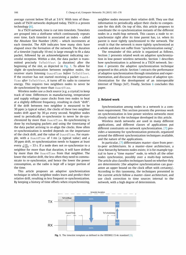
In a TSCH network, time is cut into timeslots. Timeslotsare grouped into a slotframe which continuously repeatsover time. Each timeslot is associated an index – calledthe Absolute Slot Number (ASN) – which increments ateach timeslot. The ASN indicates how many slots haveelapsed since the formation of the network. The durationof a timeslot (typically 10 ms) is large enough to fit a datapacket, followed by an acknowledgment indicating suc-cessful reception. Within a slot, the data packet is trans-mitted precisely TsTxOffset (a duration) after thebeginning of the slot, as depicted in Fig. 1. To allow forslight de-synchronization between neighbor nodes, thereceiver starts listening GuardTime before TsTxOffset.If the receiver has not started receiving a packet Guard-Time after TsTxOffset, it turns off its radio to conserveenergy. This requires two neighbors nodes to never bede-synchronized by more than GuardTime.

Wireless nodes use a clock source (e.g. a crystal) to keeptrack of time. Differences in manufacturing, temperatureand supply voltage cause clocks from two nodes to beatat a slightly different frequency, resulting in clock ‘‘drift’’.If the drift between two neighbor is measured to be30 ppm (a typical value), the clocks of these two neighbornodes drift apart by 30 ls every second. Neighbor nodesneed to periodically re-synchronize to never be de-syn-chronized by more than GuardTime. Re-synchronizing isdone by exchanging packets and using the timestamp ofthe data packet arriving to re-align the clocks. How oftenre-synchronization is needed depends on the importanceof the clock drift, and the value of GuardTime. For exam-ple, with a GuardTime of 1 ms (a typical value) and a30 ppm drift, re-synchronization needs to happen at leastevery 1 ms

30 ppm ¼ 33 s. If a node does not re-synchronize to a

neighbor for more than that duration, it will have driftedby more than the GuardTime from that neighbor. Thelower the relative drift, the less often they need to commu-nicate to re-synchronize, and hence the lower the powerconsumption, as the radio is kept off a larger portion ofthe time.

This article proposes an adaptive synchronizationtechnique in which neighbor nodes learn and predict theirrelative drift, resulting in less frequent re-synchronization.By keeping a history of time offsets when resynchronizing,

Fig. 1. The timeslot template as defined

neighbor nodes measure their relative drift. They use thatinformation to periodically adjust their clocks to compen-sate for this drift. On top of this, this article proposes tocoordinate the re-synchronization instants of the differentnodes in a multi-hop network. This causes a node to re-synchronize right after its time parent has, i.e. when itsparent is most tightly synchronized to the network. Theresult is that the network is more tightly synchronized asa whole and does not suffer from ‘‘synchronization swing’’.

The remainder of this article is organized as follows.Section 2 presents related work on adaptive synchroniza-tion in low-power wireless networks. Section 3 describeshow synchronization is achieved in a TSCH network. Sec-tion 4 presents the adaptive synchronization techniqueproposed in this article. Section 5 extracts the performanceof adaptive synchronization through simulation and exper-imentation, and discusses the importance of adaptive syn-chronization for the development of an interoperableInternet of Things (IoT). Finally, Section 6 concludes thispaper.

2. Related work

Synchronization among nodes in a network is a com-mon requirement. This section presents the previous workon synchronization in low-power wireless networks mostclosely related to the technique developed in this article.

Wireless mesh networks are used in many differentapplications, and different classes of applications putdifferent constraints on network synchronization. [7] pro-vides a taxonomy for synchronization protocols, organizedaround the different synchronization techniques available,and the nature of the applications.

In particular, [7] differentiates master–slave from peer-to-peer architectures. In a master–slave architecture, aclear hierarchy between nodes exists; it is for example typ-ical to have a ‘‘time master’’ node, to which all the othernodes synchronize, possibly over a multi-hop network.The article also classifies techniques based on whether theyare deterministic (the adaptive synchronization can guar-antee an upper bound on the clock offset with certainty).According to this taxonomy, the techniques presented inthe current article follow a master–slave architecture, anduse clock correction to time sources internal to thenetwork, with a high degree of determinism.

in the IEEE802.15.4e standard [3].

T. Chang et al. / Computer Networks 76 (2015) 165–176 167

In [8], the author indicate that, if one wants to increasethe sleep periods between resynchronization instants tominimize energy consumption, clock drift must be takeninto account. Manufacturing inaccuracies and temperaturevariation are the two major contributors to drift. Thearticle analyzes the impact of the two factors on the resyn-chronization rate, and presents a mathematical model tocalculate the resynchronization period as a function ofthe required accuracy. Similar to [8], the current articleprovides a boundary for the resynchronization periodwhich depends on the maximum acceptable time offsetbetween neighbors.

In [9], the authors provide a method for estimating thelong-term drift which minimizes the energy consumptionof the nodes. The authors use long-term empirical mea-surements to analyze the relationship between resynchro-nization rate, history of synchronization packets andestimation algorithm. They use a linear model to representrelative clock drift between two indoor neighbors nodes.The authors discuss how to predict the probability ofdifferent time errors.

The Flooding Time Synchronization Protocol [10] (FTSP)is a time synchronization method to deal with clock drift ina low-power wireless network. When using FTSP, neighbornodes estimate their relative drift by using a linear regres-sion on the past 8 time offset measurements. This estima-tion is then used to predict and reduce the apparent drift.[10] presents experimental results in which FTSP runs ontwo Mica2 nodes. They show that the nodes can keep syn-chronized within 10 ls while re-synchronizing only every10 min. The single-hop synchronization method proposedin this article (see Section 4.1) is similar to FTSP, althoughit uses only the last time-offset measurements. UnlikeFTSP, the current article applies adaptive synchronizationto TSCH networks, which adjusts synchronizing perioddynamically through learning the drift of nodes, and intro-duces a technique to synchronize a complete multi-hopnetwork (Section 4.1).

The technique presented in [11] aims at keeping a TSCHnetwork synchronized while reducing the frequency of re-synchronizations. In [11], a node measures the time ittakes for it to drift by 30 ls (a 32 kHz crystal clock tick) rel-ative to its neighbor. It then periodically applies a one-ticktime correction, using the previously calculated period.

Ref. [12] presents a detailed analysis of adaptive syn-chronization. It formalizes the relationship between calcu-lated drift accuracy and re-synchronization interval, andshows how it is possible to extend the re-synchronizationinterval to 5 min outdoors, and 1 h in a temperature-con-trolled environment [12] formalizes how the main errorof calculation of clock drift can be attributed to time cor-rection accuracy, which is itself determined by clock fre-quency. For a 32 kHz clock, the time correction accuracywould be 30 ls (one clock tick). It shows how extendingthe re-synchronization interval increases the accuracy ofthe calculated drift. Through mathematical modeling andanalysis, the paper shows that it is possible to graduallyextend the re-synchronization interval while keeping thetime offset below a given threshold.

To the best of our knowledge, and unlike the relatedwork described above, the current article is the first to

apply adaptive synchronization to a multi-hop networkas a whole. The related work presents techniques to reducethe apparent drift between neighbor nodes, i.e. they focuson single-hop synchronization. Regardless of the techniqueused, a certain amount of clock de-synchronization willalways remain. In a multi-hop setting, these inaccuraciesadd up at each hop, possibly leading to ‘‘synchronizationswing’’. This article proposes a technique to combat this.

This main contributions of this article are:

� We present a single-hop synchronization algorithm,similar to FTSP, for a node to learn and predict theclock drift to its neighbors. This reduces the apparentdrift between neighbor nodes, extending the net-work’s lifetime.

� We organize the nodes in a network as a DirectlyAcyclic Graph (DAG) built around a single time mas-ter. The DAG structure, which is loop-free by nature,assigns a time source neighbor to each node. Follow-ing the recommendations of the IETF 6TiSCH work-ing group, we propose to reuse the DAG structurebuilt by the RPL routing protocol [13].

� Each node needs to periodically send a packet to itsparent to re-synchronize. Rather than having allnodes re-synchronize at un-coordinated times, wepropose to coordinate this activity so that a nodere-synchronizes right after its parent has. Thisresults in a periodic ‘‘synchronization wave’’ movingfrom the root of the DAG outwards, resulting in tigh-ter network-wide synchronization.

� The proposed adaptive synchronization technique isimplemented in OpenWSN, and evaluated throughsimulation and real-world experimentation on mul-tiple hardware platforms. Besides showing therobustness of the approach, it also shows that itscomplexity is low, and can be implemented in ainter-operable way on off-the-shelf platforms.

3. Synchronization in IEEE802.15.4e TSCH

All nodes in a TSCH network are synchronized. When anew node joins a network, it synchronizes to it and mustkeep synchronized at all times after that. If it looses syn-chronization, it must re-join the network, which takes bothtime and energy; this is particularly problematic for nodesforwarding traffic for other nodes. This section details howsynchronization is achieved in IEEE802.15.4e TSCH. It firstdiscusses ‘‘single-hop synchronization’’ (i.e. how a nodesynchronizes to a neighbor) before highlighting the chal-lenges of keeping a multi-hop network synchronized.

3.1. Single-hop synchronization

For a node to be synchronized to a network, it mustlearn the value of the ASN of the current slot used by theother nodes in the network, and align the edges of its slotto that of the node it synchronizes to.

A node which joins the network keeps its radio on, lis-tening for an Enhanced Beacon (EB), a type of packet. EBsare periodically sent by nodes already in the network,and contain a field indicating the current ASN number.

168 T. Chang et al. / Computer Networks 76 (2015) 165–176

As soon as the joining node hears an EB, it reads and storesthe ASN field. It then increments its internal ASN value ateach new slot.

To align its slot boundaries to that of the node sendingthe EB, the joining node timestamps the instant it startedreceiving the EB. This instant is agreed upon by all thenodes in the network. It is defined in the IEEE802.15.4estandard as TsTxOffset, a duration after the beginningof the slot. The joining node knows the value ofTsTxOffset a priori, and therefore retroactively alignsits internal timers so its slot starts exactly TsTxOffset

before the reception of the EB.Once a node is part of a network, it must keep synchro-

nized to it. Since its clock drifts relative to its neighbors’, itneeds to periodically re-synchronize. Each TSCH node isassigned a time source neighbor (how it is chosen is detailedbelow) to which it must keep synchronized at all times.

There are two ways for a node to re-synchronize to itstime source neighbor, both defined in IEEE802.15.4e-2012:

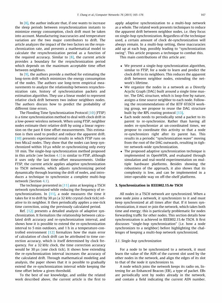
� Every time the node receives a data packet from its timesource neighbor, it timestamps the instant it startsreceiving it. Knowing TsTxOffset, it shifts it slotboundaries to match that of its time source neighbor.This is the same procedure as a joining node uses to ini-tially synchronize to the neighbor after hearing an EB.This is called ‘‘frame-based synchronization’’.� Every time the node sends a data packet to its time

source neighbor, the latter timestamps the instant itstarted receiving the packet, and indicates that valuein a field of the link-layer acknowledgment it sendsback. The sending node uses this value to realign itsclock to that of its time source neighbor. This is called‘‘ACK-based synchronization’’.

Fig. 2a and b show the two ways of re-synchronizing. Ateach re-synchronization, either frame-based or ACK-based,the receiver measures the relative de-synchronization,called offset. It is defined as the difference between themeasure reception time and TsTxOffset, its theoreticalvalue. In frame-based synchronization, the offset isapplied to the receiver’s timing; in ACK-based synchroni-zation, it is applied to the sender’s timing.

3.2. Challenges of multi-hop synchronization

The IEEE802.15.4e standard defines the mechanisms fora node to synchronize to its time source neighbor. It does

(a) Frame-based Synchronization.

Fig. 2. The two ways to synchronize defi

not detail how this time source neighbor is selected, norhow to synchronize a complete multi-hop network.IEEE802.15.4e keeps these elements out of scope, and indi-cates a ‘‘higher layer’’ is responsible for them.

The IETF 6TiSCH working group [5] was created todefine this higher layer. In the architecture of a 6TiSCH net-work, a single node plays the role of time master; all othernodes synchronize to it, possibly over multiple hops. A6TiSCH network uses RPL as its routing protocol. RPL orga-nizes the network as a Directed Acyclic Graph (DAG), inwhich each node has a routing parent. 6TiSCH recom-mends to reuse the same DAG structure for synchroniza-tion: a node’s routing parent is also its time sourceneighbor. A DAG has the advantage of being loop-free(thereby prevented synchronization loops), and since it isalready maintained by the RPL protocol, no extra signalingis needed to construct the synchronization structure.

There are subtle challenges to multi-hop synchroniza-tion, even with a DAG structure in place. A node needs toperiodically synchronize to its time source neighbor tocancel clock drift. Right before synchronizing, a node andits time source neighbor are slightly desynchronized (e.g.by 400 ls); right after synchronizing, they are tightly syn-chronized (e.g. within 30 ls). In a multi-hop case, the de-synchronization adds up with the number of hops: if there-synchronization instants of the different nodes at differ-ent hop depths are not coordinated, ‘‘synchronizationswing’’ may happen, possibly leading to the de-synchroni-zation of nodes deeper in the network.

Fig. 3 illustrates synchronization swing in the canonicalcase of a linear network of 4 nodes, in which node A is thetime source neighbor of node B, node B is the time sourceneighbor of node C, etc. The GuardTime in this networkis 1 ms, i.e. nodes can never de-synchronize by more thanthis duration. Let’s assume that, at some point in the life ofthe network, each node synchronizes right before its timesource neighbor does. It is then possible, as illustrated inthe top half of Fig. 3, that each node is desynchronizedby 400 us with respect to its time source neighbor. Let’sfurther assume that, following this configuration, nodessynchronize right after its time source neighbor, from leftto right in Fig. 3. That is, B synchronizes to A, then C syn-chronizes to B. At this point (represented in the lower halfof Fig. 3), node D and its time source neighbor are de-syn-chronized by 1200 us. Since this is more than GuardTime,node D loses synchronization.

One effective way of combating synchronization swingis for a node to learn when its time source neighbor

(b) ACK-based Synchronization.

ned in IEEE802.15.4e-2012 TSCH.

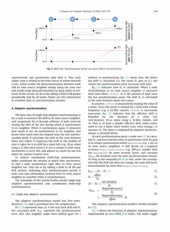
Fig. 3. Multi-hop ‘‘Synchronization Swing’’ can cause nodes to de-synchronize.

T. Chang et al. / Computer Networks 76 (2015) 165–176 169

synchronized, and synchronize right after it. Thus eachnodes’ time is related to the time source of whole network(root), which avoids the desynchronization between nodeand its time source neighbor swings along the time treeand results large desynchronization on deep nodes of net-work. In this article, we do so by adding a field in EB packetperiodically sent by all nodes. Nodes use this informationto schedule their re-synchronization instants.

4. Adaptive synchronization

The basic idea of single-hop adaptive synchronization isfor a node to measure the drift to its time source neighbor,and compensate for it through software. A node starts bystoring the ASN of the slot during which it synchronizesto its neighbor. When it synchronizes again, it measureshow much it has de-synchronized to its neighbor, andknows how much time has elapsed since the last synchro-nization point. It calculates the drift as the ratio betweenthose two values. It expresses this drift as the number ofslots it takes for it to drift by a clock tick (e.g. 30 ls whenusing a 32 kHz clock source). It sets a counter to that value,decrements it every slot, and adjusts its clocks by one tickwhen the counter reaches zero.

To achieve coordinated multi-hop synchronization,nodes coordinate the instants at which they synchronize,so that a node synchronizes right after its time sourceneighbor has. They do so by adding a field to all EB andACK packets, indicating their synchronization period. Anode uses that information received from its time sourceneighbor to schedule when it resynchronizes.

The remainder of this section further details single-hopadaptive synchronization and coordinated multi-hopsynchronization.

4.1. Single-hop adaptive synchronization

The adaptive synchronization model was first intro-duced in [12], and is presented here for completeness.

In (1), t represents time, Dr is the real clock drift and Dc

the calculated drift. Esync represent the synchronizationerror after two neighbor nodes have drifted apart for t

without re-synchronizing. Eq. (1) shows that, the betterthe drift is calculated (i.e. the closer Dc gets to Dr), theslower the synchronization error increases with time.

Eq. (2) indicates how Dc is calculated. When a noderesynchronizes to its time source neighbor, it measurestheir time offset, offset. Dt is the amount of time sincethe last synchronization point. The drift Dc is calculatedas the ratio between those two values.

In practice, offset is measured by reading the value ofa timer. Since this timer is clocked by a clock with a finitefrequency (e.g. a 32 kHz crystal), offset is necessarilyinaccurate. Eq. (3) indicates that the effective drift isbounded by the duration of a clock tick(tick duration; 30 ls when using a 32 kHz crystal), andDt. That is, to have a smaller effective drift, nodes eitherneed to use a faster clock (which costs extra energy), orincrease Dt. The latter is employed by adaptive synchroni-zation, as detailed below.

At each synchronization point, a node uses (2) to calcu-late Dc , and has to decide when to synchronize next. Its goalis to remain synchronized within GuardTime (e.g. 1 ms) toits time source neighbors. It will decide on a requiredaccuracy RequiredAccuracy (e.g. 300 ls), smaller thanthe GuardTime by some security factor, and calculateDtnext , the duration until the next synchronization instant.As long as the inequality in (4) is met, under the assump-tion that the drift rate does not change, the node will neverdesynchronize by more than RequiredAccuracy.

Esync ¼ ðDr � DcÞ � t ð1Þ

Dc ¼offsetDt

ð2Þ

jDr � Dcj 6tick duration

Dtð3Þ

Dtnext 6RequiredAccuracy

Dc

6RequiredAccuracy

offset� Dt

ð4Þ

This adaptive synchronization model is further detailedin [12].

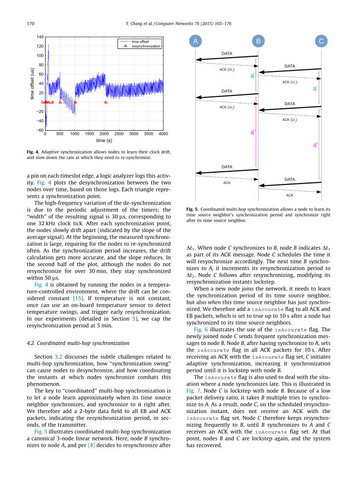
Fig. 4 shows the behavior of adaptive synchronization,implemented on two GINA [14] nodes. The nodes toggle

0 500 1000 1500 2000 2500 3000 3500 4000−60

−40

−20

0

20

40

60

80

100

120

140

time (s)

time

offs

et (u

s)

time offsetresynchronization

Fig. 4. Adaptive synchronization allows nodes to learn their clock drift,and slow down the rate at which they need to re-synchronize.

Fig. 5. Coordinated multi-hop synchronization allows a node to learn itstime source neighbor’s synchronization period and synchronize rightafter its time source neighbor.

170 T. Chang et al. / Computer Networks 76 (2015) 165–176

a pin on each timeslot edge, a logic analyzer logs this activ-ity. Fig. 4 plots the desynchronization between the twonodes over time, based on those logs. Each triangle repre-sents a synchronization point.

The high-frequency variation of the de-synchronizationis due to the periodic adjustment of the timers; the‘‘width’’ of the resulting signal is 30 ls, corresponding toone 32 kHz clock tick. After each synchronization point,the nodes slowly drift apart (indicated by the slope of theaverage signal). At the beginning, the measured synchroni-zation is large, requiring for the nodes to re-synchronizedoften. As the synchronization period increases, the driftcalculation gets more accurate, and the slope reduces. Inthe second half of the plot, although the nodes do notresynchronize for over 30 min, they stay synchronizedwithin 50 ls.

Fig. 4 is obtained by running the nodes in a tempera-ture-controlled environment, where the drift can be con-sidered constant [15]. If temperature is not constant,once can use an on-board temperature sensor to detecttemperature swings, and trigger early resynchronization.In our experiments (detailed in Section 5), we cap theresynchronization period at 5 min.

4.2. Coordinated multi-hop synchronization

Section 3.2 discusses the subtle challenges related tomulti-hop synchronization, how ‘‘synchronization swing’’can cause nodes to desynchronize, and how coordinatingthe instants at which nodes synchronize combats thisphenomenon.

The key to ‘‘coordinated’’ multi-hop synchronization isto let a node learn approximately when its time sourceneighbor synchronizes, and synchronize to it right after.We therefore add a 2-byte data field to all EB and ACKpackets, indicating the resynchronization period, in sec-onds, of the transmitter.

Fig. 5 illustrates coordinated multi-hop synchronizationa canonical 3-node linear network. Here, node B synchro-nizes to node A, and per (4) decides to resynchronize after

Dt1. When node C synchronizes to B, node B indicates Dt1

as part of its ACK message. Node C schedules the time itwill resynchronize accordingly. The next time B synchro-nizes to A, it increments its resynchronization period toDt2. Node C follows after resynchronizing, modifying itsresynchronization instants lockstep.

When a new node joins the network, it needs to learnthe synchronization period of its time source neighbor,but also when this time source neighbor has just synchro-nized. We therefore add a isAccurate flag to all ACK andEB packets, which is set to true up to 10 s after a node hassynchronized to its time source neighbors.

Fig. 6 illustrates the use of the isAccurate flag. Thenewly joined node C sends frequent synchronization mes-sages to node B. Node B, after having synchronize to A, setsthe isAccurate flag in all ACK packets for 10 s. Afterreceiving an ACK with the isAccurate flag set, C initiatesadaptive synchronization, increasing it synchronizationperiod until it is lockstep with node B.

The isAccurate flag is also used to deal with the situ-ation where a node synchronizes late. This is illustrated inFig. 7. Node C is lockstep with node B. Because of a lowpacket delivery ratio, it takes B multiple tries to synchro-nize to A. As a result, node C, on the scheduled resynchro-nization instant, does not receive an ACK with theisAccurate flag set. Node C therefore keeps resynchro-nizing frequently to B, until B synchronizes to A and Creceives an ACK with the isAccurate flag set. At thatpoint, nodes B and C are lockstep again, and the systemhas recovered.

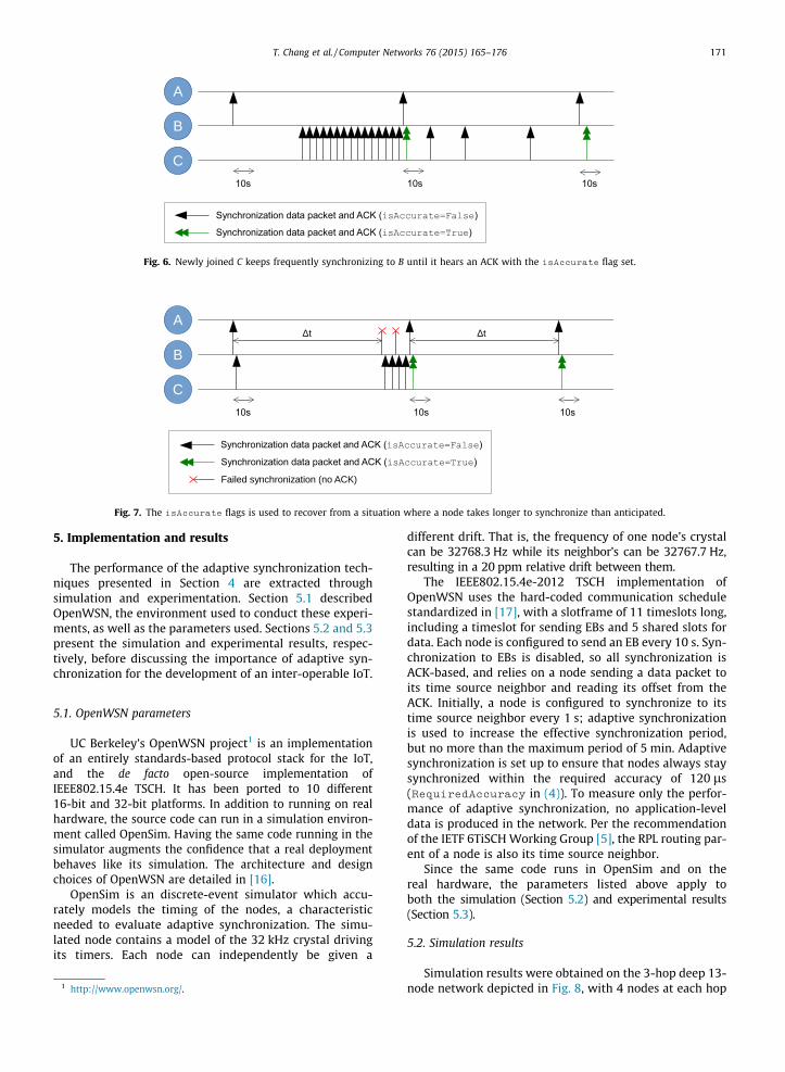
Fig. 6. Newly joined C keeps frequently synchronizing to B until it hears an ACK with the isAccurate flag set.

Fig. 7. The isAccurate flags is used to recover from a situation where a node takes longer to synchronize than anticipated.

T. Chang et al. / Computer Networks 76 (2015) 165–176 171

5. Implementation and results

The performance of the adaptive synchronization tech-niques presented in Section 4 are extracted throughsimulation and experimentation. Section 5.1 describedOpenWSN, the environment used to conduct these experi-ments, as well as the parameters used. Sections 5.2 and 5.3present the simulation and experimental results, respec-tively, before discussing the importance of adaptive syn-chronization for the development of an inter-operable IoT.

5.1. OpenWSN parameters

UC Berkeley’s OpenWSN project1 is an implementationof an entirely standards-based protocol stack for the IoT,and the de facto open-source implementation ofIEEE802.15.4e TSCH. It has been ported to 10 different16-bit and 32-bit platforms. In addition to running on realhardware, the source code can run in a simulation environ-ment called OpenSim. Having the same code running in thesimulator augments the confidence that a real deploymentbehaves like its simulation. The architecture and designchoices of OpenWSN are detailed in [16].

OpenSim is an discrete-event simulator which accu-rately models the timing of the nodes, a characteristicneeded to evaluate adaptive synchronization. The simu-lated node contains a model of the 32 kHz crystal drivingits timers. Each node can independently be given a

1 http://www.openwsn.org/.

different drift. That is, the frequency of one node’s crystalcan be 32768.3 Hz while its neighbor’s can be 32767.7 Hz,resulting in a 20 ppm relative drift between them.

The IEEE802.15.4e-2012 TSCH implementation ofOpenWSN uses the hard-coded communication schedulestandardized in [17], with a slotframe of 11 timeslots long,including a timeslot for sending EBs and 5 shared slots fordata. Each node is configured to send an EB every 10 s. Syn-chronization to EBs is disabled, so all synchronization isACK-based, and relies on a node sending a data packet toits time source neighbor and reading its offset from theACK. Initially, a node is configured to synchronize to itstime source neighbor every 1 s; adaptive synchronizationis used to increase the effective synchronization period,but no more than the maximum period of 5 min. Adaptivesynchronization is set up to ensure that nodes always staysynchronized within the required accuracy of 120 ls(RequiredAccuracy in (4)). To measure only the perfor-mance of adaptive synchronization, no application-leveldata is produced in the network. Per the recommendationof the IETF 6TiSCH Working Group [5], the RPL routing par-ent of a node is also its time source neighbor.

Since the same code runs in OpenSim and on thereal hardware, the parameters listed above apply toboth the simulation (Section 5.2) and experimental results(Section 5.3).

5.2. Simulation results

Simulation results were obtained on the 3-hop deep 13-node network depicted in Fig. 8, with 4 nodes at each hop

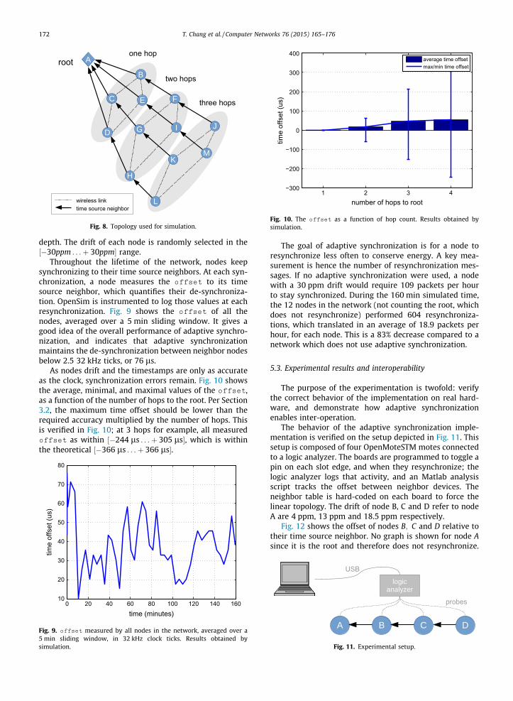
Fig. 8. Topology used for simulation.

1 2 3 4−300

−200

−100

0

100

200

300

400

number of hops to root

time

offs

et (u

s)

average time offsetmax/min time offset

Fig. 10. The offset as a function of hop count. Results obtained bysimulation.

172 T. Chang et al. / Computer Networks 76 (2015) 165–176

depth. The drift of each node is randomly selected in the½�30ppm . . .þ 30ppm� range.

Throughout the lifetime of the network, nodes keepsynchronizing to their time source neighbors. At each syn-chronization, a node measures the offset to its timesource neighbor, which quantifies their de-synchroniza-tion. OpenSim is instrumented to log those values at eachresynchronization. Fig. 9 shows the offset of all thenodes, averaged over a 5 min sliding window. It gives agood idea of the overall performance of adaptive synchro-nization, and indicates that adaptive synchronizationmaintains the de-synchronization between neighbor nodesbelow 2.5 32 kHz ticks, or 76 ls.

As nodes drift and the timestamps are only as accurateas the clock, synchronization errors remain. Fig. 10 showsthe average, minimal, and maximal values of the offset,as a function of the number of hops to the root. Per Section3.2, the maximum time offset should be lower than therequired accuracy multiplied by the number of hops. Thisis verified in Fig. 10; at 3 hops for example, all measuredoffset as within ½�244 ls . . .þ 305 ls�, which is withinthe theoretical ½�366 ls . . .þ 366 ls�.

0 20 40 60 80 100 120 140 16010

20

30

40

50

60

70

80

time (minutes)

time

offs

et (u

s)

Fig. 9. offset measured by all nodes in the network, averaged over a5 min sliding window, in 32 kHz clock ticks. Results obtained bysimulation.

The goal of adaptive synchronization is for a node toresynchronize less often to conserve energy. A key mea-surement is hence the number of resynchronization mes-sages. If no adaptive synchronization were used, a nodewith a 30 ppm drift would require 109 packets per hourto stay synchronized. During the 160 min simulated time,the 12 nodes in the network (not counting the root, whichdoes not resynchronize) performed 604 resynchroniza-tions, which translated in an average of 18.9 packets perhour, for each node. This is a 83% decrease compared to anetwork which does not use adaptive synchronization.

5.3. Experimental results and interoperability

The purpose of the experimentation is twofold: verifythe correct behavior of the implementation on real hard-ware, and demonstrate how adaptive synchronizationenables inter-operation.

The behavior of the adaptive synchronization imple-mentation is verified on the setup depicted in Fig. 11. Thissetup is composed of four OpenMoteSTM motes connectedto a logic analyzer. The boards are programmed to toggle apin on each slot edge, and when they resynchronize; thelogic analyzer logs that activity, and an Matlab analysisscript tracks the offset between neighbor devices. Theneighbor table is hard-coded on each board to force thelinear topology. The drift of node B, C and D refer to nodeA are 4 ppm, 13 ppm and 18.5 ppm respectively.

Fig. 12 shows the offset of nodes B; C and D relative totheir time source neighbor. No graph is shown for node Asince it is the root and therefore does not resynchronize.

Fig. 11. Experimental setup.

0 200 400 600 800 1000−300

−200

−100

0

100

200

300

Time (s)

time

offs

et (u

s)

time offsetresynchronization

(a) Node B

0 200 400 600 800 1000−300

−200

−100

0

100

200

300

Time (s)

time

offs

et (u

s)

time offsetresynchronization

(b) Node C

0 200 400 600 800 1000−300

−200

−100

0

100

200

300

Time (s)

time

offs

et (u

s)

time offsetresynchronization

(c) Node D

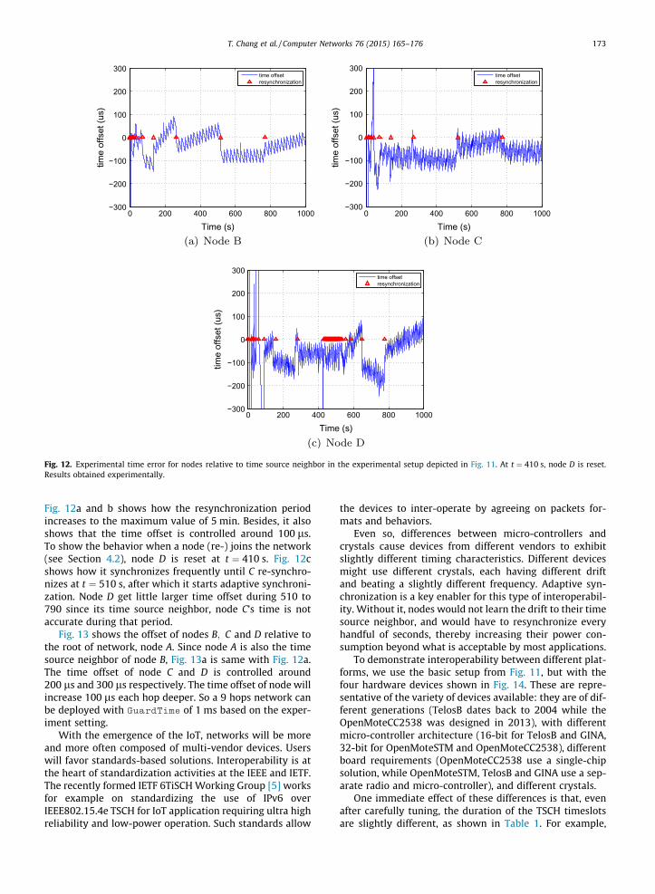
Fig. 12. Experimental time error for nodes relative to time source neighbor in the experimental setup depicted in Fig. 11. At t ¼ 410 s, node D is reset.Results obtained experimentally.

T. Chang et al. / Computer Networks 76 (2015) 165–176 173

Fig. 12a and b shows how the resynchronization periodincreases to the maximum value of 5 min. Besides, it alsoshows that the time offset is controlled around 100 ls.To show the behavior when a node (re-) joins the network(see Section 4.2), node D is reset at t ¼ 410 s. Fig. 12cshows how it synchronizes frequently until C re-synchro-nizes at t ¼ 510 s, after which it starts adaptive synchroni-zation. Node D get little larger time offset during 510 to790 since its time source neighbor, node C’s time is notaccurate during that period.

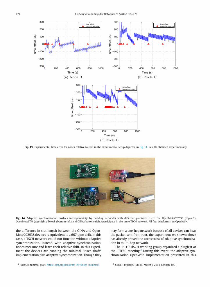
Fig. 13 shows the offset of nodes B; C and D relative tothe root of network, node A. Since node A is also the timesource neighbor of node B, Fig. 13a is same with Fig. 12a.The time offset of node C and D is controlled around200 ls and 300 ls respectively. The time offset of node willincrease 100 ls each hop deeper. So a 9 hops network canbe deployed with GuardTime of 1 ms based on the exper-iment setting.

With the emergence of the IoT, networks will be moreand more often composed of multi-vendor devices. Userswill favor standards-based solutions. Interoperability is atthe heart of standardization activities at the IEEE and IETF.The recently formed IETF 6TiSCH Working Group [5] worksfor example on standardizing the use of IPv6 overIEEE802.15.4e TSCH for IoT application requiring ultra highreliability and low-power operation. Such standards allow

the devices to inter-operate by agreeing on packets for-mats and behaviors.

Even so, differences between micro-controllers andcrystals cause devices from different vendors to exhibitslightly different timing characteristics. Different devicesmight use different crystals, each having different driftand beating a slightly different frequency. Adaptive syn-chronization is a key enabler for this type of interoperabil-ity. Without it, nodes would not learn the drift to their timesource neighbor, and would have to resynchronize everyhandful of seconds, thereby increasing their power con-sumption beyond what is acceptable by most applications.

To demonstrate interoperability between different plat-forms, we use the basic setup from Fig. 11, but with thefour hardware devices shown in Fig. 14. These are repre-sentative of the variety of devices available: they are of dif-ferent generations (TelosB dates back to 2004 while theOpenMoteCC2538 was designed in 2013), with differentmicro-controller architecture (16-bit for TelosB and GINA,32-bit for OpenMoteSTM and OpenMoteCC2538), differentboard requirements (OpenMoteCC2538 use a single-chipsolution, while OpenMoteSTM, TelosB and GINA use a sep-arate radio and micro-controller), and different crystals.

One immediate effect of these differences is that, evenafter carefully tuning, the duration of the TSCH timeslotsare slightly different, as shown in Table 1. For example,

0 200 400 600 800 1000−300

−200

−100

0

100

200

300

Time (s)

time

offs

et (u

s)

time offsetresynchronization

(a) Node B

0 200 400 600 800 1000−300

−200

−100

0

100

200

300

Time (s)

time

offs

et (u

s)

time offsetresynchronization

(b) Node C

0 200 400 600 800 1000−300

−200

−100

0

100

200

300

Time (s)

time

offs

et (u

s)

time offsetresynchronization

(c) Node D

Fig. 13. Experimental time error for nodes relative to root in the experimental setup depicted in Fig. 11. Results obtained experimentally.

Fig. 14. Adaptive synchronization enables interoperability by building networks with different platforms. Here the OpenMoteCC2538 (top-left),OpenMoteSTM (top-right), TelosB (bottom-left) and GINA (bottom-right) participate in the same TSCH network. All four platforms run OpenWSN.

174 T. Chang et al. / Computer Networks 76 (2015) 165–176

the difference in slot length between the GINA and Open-MoteCC2538 devices is equivalent to a 667 ppm drift. In thiscase, a TSCH network could not function without adaptivesynchronization. Instead, with adaptive synchronization,nodes measure and learn their relative drift. In this experi-ment the devices are running the minimal 6tisch draft2

implementation plus adaptive synchronization. Though they

2 6TISCH minimal draft, https://ietf.org/doc/draft-ietf-6tisch-minimal/.

may form a one-hop network because of all devices can hearthe packet sent from root, the experiment we shown abovehas already proved the correctness of adaptive synchroniza-tion in multi-hop network.

The IETF 6TiSCH working group organized a plugfest atthe IETF89 meeting.3 During this event, the adaptive syn-chronization OpenWSN implementation presented in this

3 6TiSCH plugfest, IETF89, March 6 2014, London, UK.

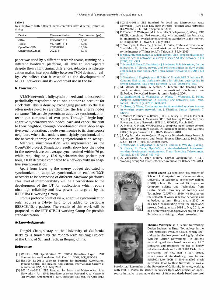
Table 1Four hardware with different micro-controller have different feature ontiming.

Device Micro-controller Slot duration (ls)

GINA MSP430F2618 15,000TelosB MSP430F1611 15,000OpenMoteSTM STM32F103 15,004OpenMoteCC2538 CC2538 15,010

T. Chang et al. / Computer Networks 76 (2015) 165–176 175

paper was used by 5 different research teams, running on 7different hardware platforms, all able to inter-operatedespite their slight timing differences. Adaptive synchroni-zation makes interoperability between TSCH devices a real-ity. We believe that it essential to the development of6TiSCH networks, and its widespread use in the IoT.

6. Conclusion

A TSCH network is fully synchronized, and nodes need toperiodically resynchronize to one another to account forclock drift. This is done by exchanging packets, so the lessoften nodes need to resynchronize, the less energy nodesconsume. This article presents an adaptive synchronizationtechnique composed of two part. Through ‘‘single-hop’’adaptive synchronization, nodes learn and cancel the driftto their neighbor. Through ‘‘coordinated’’ multi-hop adap-tive synchronization, a node synchronize to its time sourceneighbors when that node is most tightly synchronized tothe network, thereby combating ‘‘synchronization swing’’.

Adaptive synchronization was implemented in theOpenWSN project. Simulation results show how the nodesin the network are on average synchronized within 76 ls,while requiring only 18.9 synchronization packets perhour, a 83% decrease compared to a network with no adap-tive synchronization.

Apart from lowering the energy budget dedicated tosynchronization, adaptive synchronization enables TSCHnetworks to be composed of different hardware platforms.This level of interoperability will be a cornerstone to thedevelopment of the IoT for applications which requireultra-high reliability and low-power, as targeted by theIETF 6TiSCH working Group.

From a protocol point of view, adaptive synchronizationonly requires a 2-byte field to be added to particularIEEE802l.15.4e packets. The results of this work will beproposed to the IETF 6TiSCH working Group for possiblestandardization.

Acknowledgments

Tengfei Chang’s stay at the University of California,Berkeley is funded by the ‘‘Short-Term Visiting Project’’of the Univ. of Sci. and Tech. in Beijing, China.

References

[1] WirelessHART Specification 75: TDMA Data-Link Layer, HARTCommunication Foundation Std., Rev. 1.1, 2008, hCF_SPEC-75.

[2] ISA-100.11a-2011: Wireless Systems for Industrial Automation:Process Control and Related Applications, International Society ofAutomation (ISA) Std., May 2011.

[3] 802.15.4e-2012: IEEE Standard for Local and Metropolitan AreaNetworks – Part 15.4: Low-Rate Wireless Personal Area Networks(LR-WPANs) Amendment 1: MAC Sublayer, IEEE Std., 16 April 2012.

[4] 802.15.4-2011: IEEE Standard for Local and Metropolitan AreaNetworks – Part 15.4: Low-Rate Wireless Personal Area Networks(LR-WPANs), IEEE Std., 5 September 2011.

[5] P. Thubert, T. Watteyne, M.R. Palattella, X. Vilajosana, Q. Wang, IETF6TSCH: combining IPv6 connectivity with industrial performance,in: International Workshop on Extending Seamlessly to the Internetof Things (esIoT), Taiwan, 3–5 July 2013.

[6] T. Watteyne, L. Doherty, J. Simon, K. Pister, Technical overview ofSmartMesh IP, in: International Workshop on Extending Seamlesslyto the Internet of Things (esIoT), Taiwan, 3–5 July 2013.

[7] B. Sundararaman, U. Buy, A. Kshemkalyani, Clock synchronization forwireless sensor networks: a survey, Elsevier Ad Hoc Network. 3 (3)(2005) 281–323.

[8] T. Schmid, R. Shea, Z. Charbiwala, J. Friedman, M.B. Srivastava, On theinteraction of clocks, power, and synchronization in duty-cycledembedded sensor nodes, ACM Trans. Sensor Networks (TOSN) 7 (3)(2010).

[9] S. Ganeriwal, I. Tsigkogiannis, H. Shim, V. Tsiatsis, M.B. Srivastava, D.Ganesan, Estimating clock uncertainty for efficient duty-cycling insensor networks, IEEE Trans. Network. 17 (3) (2009) 843–856.

[10] M. Maroti, B. Kusy, G. Simon, A. Ledeczi, The flooding timesynchronization protocol, in: international Conference onEmbedded Networked Sensor Systems (SenSys), 2004.

[11] D. Stanislowski, X. Vilajosana, Q. Wang, T. Watteyne, K. Pister,Adaptive synchronization in IEEE802.15.4e networks, IEEE Trans.Indust. Inform. 9 (2) (2013) 600–608.

[12] T. Chang, Q. Wang, Compensation for time-slotted synchronizationin wireless sensor network, Int. J. Distribut. Sensor Networks 7(2014).

[13] T. Winter, P. Thubert, A. Brandt, J. Hui, R. Kelsey, P. Levis, K. Pister, R.Struik, J. Vasseur, R. Alexander, RPL: IPv6 Routing Protocol for Low-Power and Lossy Networks, IETF Std. RFC6550, March 2012.

[14] A. Mehta, K. Pister, WARPWING: a complete open source controlplatform for miniature robots, in: Intelligent Robots and Systems(IROS), Taipei, Taiwan, IEEE, 18–22 October 2010.

[15] J.R. Vig, Introduction to Quartz Frequency Standards, Army ResearchLaboratory, Electronics and Power Sources Directorate, Tech. Rep.SLCET-TR-92-1 (Rev. 1), October 1992.

[16] T. Watteyne, X. Vilajosana, B. Kerkez, F. Chraim, K. Weekly, Q. Wang,S. Glaser, K. Pister, OpenWSN: a standards-based low-powerwireless development environment, Trans. Emerging Telecommun.Technol. 23 (5) (2012) 480–493.

[17] X. Vilajosana, K. Pister, Minimal 6TiSCH Configuration, 6TiSCHWorking Group Std. Draft-ietf-6tisch-minimal-03, October 26, 2014.

Tengfei Chang is a candidate Ph.D student ofSchool of Computer and Communication,University of Science & Technology Beijing(USTB), China. He received BS degree inComputer Science and Technology fromCentral South University of Forestry andTechnology (CSUFT) in 2010. He focuses onthe research of wireless sensor networks andembedded systems. Since January 2012, hehas been collaborating with the OpenWSNproject. During January 2014 to May 2014, hehad been working on OpenWSN project in UCBerkeley as a visiting student researcher.

Thomas Watteyne is a Senior NetworkingDesign Engineer at Linear Technology, in theDust Networks Product Group, which spe-cializes in ultralow power and highly reliableWireless Sensor Networking. He designsnetworking solutions based on a variety of IoTstandards and promotes the use of highlyreliable standards such as IEEE802.15.4e. He isco-chairing the new IETF 6TiSCH group,which aims at standardizing how to useIEEE802.15.4e TSCH in IPv6-enabled meshnetworks. Prior to Dust Network, he was a

Postdoctoral Researcher at the University of California, Berkeley, workingwith Prof. K. Pister. He started Berkeley’s OpenWSN project, an open-source initiative to promote the use of fully standards-based protocol

176 T. Chang et al. / Computer Networks 76 (2015) 165–176

stacks in M2M applications. He received the Ph.D. degree in computerscience (2008) and the M.Sc. degree in telecommunications (2005) fromINSA Lyon, France.

Kristofer S.J. Pister received his B.A. inApplied Physics from UCSD in 1986, and hisM.S. and Ph.D. in Electrical Engineering fromUC Berkeley in 1989 and 1992. From 1992 to1997 he was an Assistant Professor of Elec-trical Engineering at UCLA where he devel-oped the graduate MEMS curriculum, andcoined the phrase Smart Dust. Since 1996 hehas been a professor of Electrical Engineeringand Computer Sciences at UC Berkeley. In2003 and 2004 he was on leave from UCB asCEO and then CTO of Dust Networks, a com-

pany he founded to commercialize wireless sensor networks. He partic-ipated in the creation of several wireless sensor networking standards,including Wireless HART (IEC62591), IEEE 802.15.4e, ISA100.11A, and

IETF RPL. He has participated in many government science and technol-ogy programs, including DARPA ISAT and the Defense Science StudyGroup, and he is currently a member of the Jasons. His research interestsinclude MEMS, micro robotics, and low power circuits.

Qin Wang is a Professor with the SchoolComputer and Communication, University ofScience and Technology Beijing (USTB), China.She received the B.S., M.S., and Ph.D. degreesin computer science and engineering fromUSTB in 1982, Peking University in 1985, andUSTB in 1998, respectively. She joined USTB in1985, became Full Professor in 2000. As aVisiting Scientist (2005–2006) in the Electri-cal Engineering and Computer ScienceDepartment, Cornell University, NY, and Vis-iting Researcher (2006–2007) in the Electrical

Engineering and Computer Science Department, Harvard University,Cambridge, MA, her research and contributions were on wireless sensornetwork technology and related power consumption modeling from both

device and network system perspective. Recent years, she has focused onlow power wireless sensor networks and MPSoC (multiprocessor System-on-Chip) technology in communications and networking systems. SinceJanuary 2012, she has been working on OpenWSN project in UC Berkeleyas a visiting professor. She has been involved in international wirelessnetwork standard development since 2007, including ISA100.11a, IEEE802.15.4e, and industrial wireless standard WIA-PA proposed to IEC byChina.