adding indonesia to the global projection model · adding indonesia to the global projection model...
TRANSCRIPT

Adding Indonesia to the Global Projection Model
Michal Andrle, Charles Freedman,
Roberto Garcia-Saltos, Danny Hermawan, Douglas Laxton,
and Haris Munandar.
WP/09/253

© 2009 International Monetary Fund WP/09/253 IMF Working Paper Research Department
Adding Indonesia to the Global Projection Model1
Prepared by Michal Andrle, Charles Freedman, Roberto Garcia-Saltos, Danny Hermawan, Douglas Laxton, and Haris Munandar.
November 2009
Abstract
This Working Paper should not be reported as representing the views of the IMF. The views expressed in this Working Paper are those of the author(s) and do not necessarily represent those of the IMF or IMF policy. Working Papers describe research in progress by the author(s) and are published to elicit comments and to further debate.
This is the fifth of a series of papers that are being written as part of a larger project to estimate a small quarterly Global Projection Model (GPM). The GPM project is designed to improve the toolkit to which economists have access for studying both own-country and cross-country linkages. In this paper, we add Indonesia to a previously estimated small quarterly projection model of the US, euro area, and Japanese economies. The model is estimated with Bayesian techniques, which provide a very efficient way of imposing restrictions to produce both plausible dynamics and sensible forecasting properties. JEL Classification Numbers: C51; E31; E52 Keywords: Macroeconomic Modeling; Bayesian Estimation, Monetary Policy Author’s E-Mail Address: [email protected]@imf.org,
1 C. Freedman is Scholar in Residence in the Economics Department, Carleton University, Ottawa, Canada. The authors wish to thank Olivier Blanchard, Charles Collyns, Ondra Kamenik, Robert Rennhack and our colleagues at other policymaking institutions for encouraging us to do this work. We also gratefully acknowledge the invaluable support of Heesun Kiem, Ioan Carabenciov, Susanna Mursula, Carolina Saizar, Ben Sutton and Laura Leon. The views expressed here are those of the authors and do not necessarily reflect the position of the International Monetary Fund or Bank of Indonesia. Correspondence: [email protected].

2
Contents Page I. Introduction ....................................................................................................................4 A. Background ...........................................................................................................4 B. A Brief Outline of Indonesian Economic Developments Over The Sample Period ....................................................................................5 II. Benchmark Model ..........................................................................................................8 A. Background ...........................................................................................................8 B. The Specification of The Model .........................................................................12 B.1 Observable variables and data definitions ..................................13 B.2 Stochastic processes and model definitions ................................14 B.3 Behavorial equations ...................................................................16 B.4 Cross correlations of disturbances ..............................................20 III. Extending the Model to Include Financial-Real Linkages ..........................................21 A. Background .........................................................................................................21 B. Model Specification Incorporating the US Bank Lending Tightening Variable ................................................................................24 IV. Modifications of the Model for the Indonesian Economy ...........................................26 V. Confronting the Model with the Data ..........................................................................29 A. Bayesian Estimation............................................................................................29 B. Results .................................................................................................................31 B.1 Estimates of coeficients ..............................................................31 B.2 Estimates of standard deviation of structural shocks and cross correlations .........................................................33 B.3 RMSEs ........................................................................................34 B.4 Impulse response functions .........................................................34 VI. Concluding Remarks ....................................................................................................36 References ................................................................................................................................38 Appendix: GPM Data Definitions ...........................................................................................41 Figures 1. Indonesia – Historical Data [1] ....................................................................................42 2. Indonesia – Historical Data [2] ....................................................................................43

3
3. Indonesia – Historical Data [3] ....................................................................................44 4. Comparison CDS Emerging Countries ........................................................................45 5. Indonesia Historical Inflation Graph ...........................................................................47 6. Domestic Demand Shock .............................................................................................51 7. Domestic Price Shock ..................................................................................................52 8. Domestic Interest Rate Shock ......................................................................................53 9. Domestic Real Exchange Rate Shock ..........................................................................54 10. Shock to the Domestic Target Rate of Inflation ..........................................................55 11. Demand Shock in the US .............................................................................................56 12. BLT Shock in the US ...................................................................................................57 Tables 1. Results from Posterior Maximization ..........................................................................46 2. Results from Posterior Parameters (standard deviation of structural shocks) .............48 3. Results from Posterior Parameters (correlation of structural shocks) .........................49 4. Root Mean Squared Errors...........................................................................................50

4
I. Introduction
A. Background
This study is the �fth of a series of studies designed to develop a full global projection
model. The �rst study in the series, �A small quarterly projection model of the US
economy�(Carabenciov and others, 2008a), set out a closed economy version of the
model and applied it to the US economy using Bayesian estimation techniques. It
incorporated a �nancial variable for the US economy, enabling us to see the e¤ects of
changes in this variable on US output and in�ation. The second in the series, �A small
quarterly multi-country projection model�(Carabenciov and others, 2008b), extended
the model to an open economy. It set out a small quarterly projection model of the US,
euro area, and Japanese economies to illustrate the way that such models can be used
to understand past economic developments and to forecast future developments in a
multi-country setting. It also incorporated the �nancial variable for the US economy,
enabling us to see the e¤ects of changes in this variable on the US economy and on the
other economies. The third paper in the series, �A Small Quarterly Multi-Country
Projection Model With Financial-Real Linkages and Oil Prices�(Carabenciov and
others, 2008c), added oil prices to the three country model. This permitted us to
examine the e¤ects of temporary and permanent shocks to the level and growth rate of
oil prices on the three economies. The fourth paper in the series,�Adding Latin
America to the Global Projection Model�(Canales-Kriljenko and others, 2009) added
the aggregate of the �ve in�ation-targeting Latin American economies (Brazil, Chile,
Colombia, Mexico and Peru) to the previously-estimated three country model without
oil.
In this paper, we add a model of the Indonesian economy to the previously-estimated
three country model without oil presented in Carabenciov and others (2008b). The
usefulness of a multi-country framework to analyze economic developments in Indonesia
and to provide a framework for projection scenarios has been enhanced by the large
increase in, and the rather complex dynamics of, trade and �nancial �ows experienced
by Indonesia in recent years. The extended model allows us to examine the e¤ects on
Indonesia of domestic demand and supply shocks, and also permits us to examine the
e¤ects on the Indonesian economy of shocks in the world�s largest economies.

5
While the emphasis in this paper is on the results of the extended model, a companion
�how to�paper is currently being written that will provide a guide to central banks in
other countries that would like to add a small model of their own economy to the model
of the three large economies. Among the issues addressed in that paper will be how to
add new countries to the basic large economy model in a way that is most e¢ cient.
The studies completed thus far are preparatory to the next steps in our research agenda
��rst, to incorporate a more sophisticated oil sector with global demand and supply for
oil; second, to extend the model to include �nancial variables in countries other than
the United States; and third, to develop a small quarterly Global Projection Model
(GPM) that will integrate a number of large and small country models into a single
global model that can be used for global economic projections. Such a model would
include the United States, the euro area, Japan, oil exporters, China, emerging Asia
excluding China, and the rest of the world.
B. A Brief Outline of Indonesian Economic Developments Over the
Sample Period
This section brie�y discusses Indonesian economic developments since 2000 to help set
the scene for the analysis of the Indonesian economy in this study.1 The key variables
for the Indonesian economy over the 2000-2008 period are set out in �gures 1 to 3.
Indonesia is an open emerging market economy. In the year 2008, exports and imports
were about 30% and 29% of GDP at current market prices respectively, and about 50%
and 40% of real GDP at 2000 market prices. Nonetheless, Indonesia is still the second
most closed economy in the region, and therefore relatively less exposed than others to
a slump in foreign demand.
From the economic perspective, its history for the latter part of the 1990s and much of
this decade has involved the recovery from the economic devastation of the Southeast
Asian crisis of 1997 to 1998. Prior to that episode, the Indonesian economy had been
growing at about 7% to 8% on average. In 1998, during the crisis, the Indonesian
1This section is largely based on Goeltom, 2007, chapters 3 and 5 and Bank Indonesia Annual Reports(2003 through 2007).

6
economy declined by about 13%, and in the recovery from that decline it posted
relatively low growth rates, just under 5% on average, for a number of years. Since the
middle of this decade, real GDP growth has picked up again and has tended to be over
5.5% for much of the time.
On the in�ation side, the trend in Indonesia in the 1990s was for in�ation to be in the
high single digits. The collapse in the exchange rate in 1997 led to a very sharp spike in
in�ation to about 82% in September 1998 before the rate fell back into the single digit
range. Since 2000, headline in�ation has ranged between 6% and 13%, with no clear
downward trend, while core in�ation has hovered around 6% to 8% after falling into the
single digit range in 2002. The reduction in the subsidy to oil prices in an environment
of sharply rising world oil prices led to increases in both headline and, to a lesser
extent, core in�ation in 2005-06. This episode is of particular interest in the context of
the conduct of monetary policy in Indonesia and will be discussed further below. The
recent sharp rise in commodity prices, particularly oil prices, has led to a considerable
pickup in headline in�ation, which reached 15.6% in the second quarter of 2008.
After appreciating from above 10,000 rupiah to the US dollar in the early part of the
decade to the mid-8,000 range by 2003, the Indonesian currency depreciated again to
the high 9,000s in 2005, before settling down in the low 9,000s over the subsequent
period, until recently. After initially weathering the global �nancial crisis without much
di¢ culty, the rupiah rose sharply from about 9,200 to about 12,150 to the dollar in the
fourth quarter of 2008 as global risk aversion became increasingly widespread. The real
exchange rate vis-à-vis the three major economies (United States, the euro area and
Japan) shows a trend to real appreciation on average over much of the decade. This is
not unexpected in light of the Balassa-Samuelson insight that emerging economies are
likely to have higher productivity growth in tradables relative to nontradables as
compared to industrialized economies. For much of the period, this has shown up in
Indonesia as a higher rate of CPI in�ation than in its large industrialized trading
partners (United States, euro area, Japan), combined with a relatively stable e¤ective
nominal exchange rate. An extension of the real e¤ective exchange rate data to include
the nine most important trading partners for Indonesia shows a similar pattern to the
3-country data.
The post-crisis situation has been characterized by continuing attempts to improve the

7
economic and �nancial infrastructure of the country. Much concern has been expressed
over the weakness of real investment in the economy, since such investment is an
essential prerequisite for a pickup of potential output growth.2 Over the period, the
authorities have also undertaken a large number of initiatives to strengthen the
�nancial sector and avoid the problems that made that sector so vulnerable during the
crisis. In spite of the progress in this area, Indonesia still appears to be more vulnerable
than many of its neighbors as shown by the credit default swap (CDS) for Indonesia,
which is at present appreciably higher than that of its neighbors (see �gure 4).
As far as the conduct of monetary policy is concerned, the Indonesian government
announced in�ation targets in July 2005 of 6%, 5.5% and 5% for the years 2005 to 2007
in the context of the regime shift to an in�ation targeting framework. Each of the
targets had a band of +/-1% attached to it. Following the increase in headline in�ation
over 2005 (to be discussed further below), the government announced in March 2006
that the in�ation targets for 2006 to 2008 would be 8%, 6%, and 5% (again with a
+/-1% band). And in June 2008, the government recon�rmed the 2008 target at 5%
and extended the targets to 4.5% for 2009 and 4% for 2010.
The Bank Indonesia (BI) rate (a reference rate introduced following the establishment
of the in�ation targeting framework) was increased appreciably in the early part of the
decade to deal with the lingering in�ation pressures of the post-crisis period. After
falling to below 8% as in�ation pressures subsided, it was raised again, to over 12%, in
early 2006. The episode of 2005 and 2006 is of particular interest in the context of a
discussion of monetary policy in Indonesia. Oil prices started to increase in early 2004
and the upward pressure continued until early 2006. Given the ceiling on domestic oil
prices to households, the increased level of the subsidy in the face of higher world oil
prices impinged strongly on the government budget and the government reduced the
size of the subsidy in October 2005. Thus, the result of the pressure from higher world
oil prices was an appreciable rise in core in�ation, since the industrial use of oil had not
been subsidized, and a much sharper increase in headline in�ation as the price of oil in
the regulated/subsidized part of the economy was increased. In order to prevent the
in�ationary pressures from accelerating, Bank Indonesia raised the BI rate by more
2In addition to giving rise to higher standards of living, higher potential output growth would permitmore rapid aggregate demand growth without creating in�ationary pressures.

8
than 4 percentage points, from below 8% to above 12%, and both core and headline
in�ation fell back through 2006. Our interpretation of the ability of the monetary
authorities to constrain in�ation with an increase in interest rates that was much less
than the increase in headline in�ation is that the shock to headline in�ation did not
feed into expected in�ation on a one-to-one basis, as might have been the case in the
past. Rather, there was some increase in expected in�ation that required a
countervailing interest rate increase, but it was considerably less than the increase in
the headline in�ation rate. The increase in the real BI rate with respect to the core
in�ation rate and its decline with respect to the headline in�ation rate suggest that
Bank Indonesia has developed some credibility but that there is considerable room for
credibility to increase further.
II. Benchmark Model
A. Background
In recent years, the IMF has developed two main types of macroeconomic models �
dynamic stochastic general equilibrium (DSGE) models and small quarterly projection
models (QPMs) �that it has used to analyze economic behavior and to forecast future
developments. The DSGE models are based on theoretical underpinnings and have
been found to be very useful in analyzing the e¤ects of structural changes in the
economy, as well as the e¤ects of longer-term developments such as persistent �scal
de�cits and current account de�cits.3 And multi-country variants of these models have
allowed researchers to analyze the e¤ects of shocks in one country on economic
variables in other countries. The small quarterly projection models use four or �ve
behavioral equations to characterize the macroeconomic structure of an economy in a
way that is both easy to use by modelers and comprehensible to policymakers. They
focus on the key macroeconomic variables in the economy �typically output, in�ation,
a short-term interest rate, and sometimes the exchange rate and/or the unemployment
rate. By virtue of their relatively simple and readily understandable structure, they
have been used for forecasting and policy analysis purposes in central banks and by
3See Botman and others (2007) for a summary of the applications using these models.

9
country desks in the IMF.4 In the past, the parameters of such models have been
calibrated on the basis of the knowledge of country experts of the economic structure of
the country being studied and that of similar countries.
In the series of papers cited earlier and in this paper, a number of important elements
or extensions are being applied to the basic model. First, in all the papers in the series,
Bayesian techniques are used to estimate the parameters of the model. Bayesian
methods allow researchers to input their priors into the model and then to confront
them with the data, in order to determine whether their priors are more or less
consistent with the data. Although regime shifts in recent years (most notably, the
anchoring of in�ation expectations to a formal or informal target in many countries)
limit the time series to relatively short periods, the estimation approach taken in these
papers will be increasingly useful over time as the lengths of usable time series are
extended.
Second, the number of countries in the model has continually been expanded. The �rst
paper examined the US economy. In the second and third papers, we expanded the
model to three economies �United States, the Euro area, and Japan. The fourth paper
added Latin America to the three economy model, while this paper adds Indonesia to
the three economy model. In a future paper, the small quarterly models of a number of
countries (United States, the euro area, Japan, oil-exporting countries, China, emerging
Asia excluding China, and the rest of the world) will be integrated into a small
quarterly Global Projection Model (GPM) that covers the entire world economy, which
will enable researchers to analyze the e¤ects on a number of countries of shocks in one
country and of global shocks. Moreover, the model will be programmed in such way
that researchers will be able to add other countries to the model in a relatively
straightforward manner. Such models will give forecasters a new tool to assist them in
preparing worldwide forecasts and in carrying out alternative policy simulations in the
global context. There is strong demand for such an empirically based multi-country
model, both for IMF surveillance work and for helping central bank forecasters to assess
4See Berg, Karam, and Laxton (2006a,b) for a description of the basic model as well as Epstein andothers (2006) and Argov and others (2007) for examples of applications and extensions. Currently, Fundsta¤ are using the model to support forecasting and policy analysis and to better structure their dialoguewith member countries. A number of in�ation-targeting central banks have used similar models as anintegral part of their Forecasting and Policy Analysis Systems� see Coats, Laxton and Rose (2003) fora discussion about how such models are used in in�ation-targeting countries.

10
the external environment in preparing their projections. Large-scale DSGE models
show promise in this regard, but we are years away from developing empirically-based
multi-country versions of these models. While global VARs (GVARs) have been
developed for forecasting exercises, they are not very useful for policy analysis because
they lack the identi�cation restrictions necessary to obtain plausible impulse response
functions or to properly identify policy reaction functions.
Third, given the importance in recent years and at present of �nancial-real linkages, we
have been experimenting with �nancial variables that might be helpful in explaining
economic developments and in forecasting future movements of the economy. Thus far,
we have used a single �nancial variable, a US bank lending tightening measure (BLTus),
which contributed importantly to the explanation of movements of the US economy
over the sample period and also improved out-of-sample forecasting. In future papers
we will broaden the use of �nancial variables to include a number of �nancial measures
of risk in the United States and other countries.
Fourth, commodity prices are being incorporated into the model. In the third paper we
extended the model to include oil prices. On a number of occasions since 1973, sharp
increases or decreases in oil prices have had an important e¤ect on output and in�ation
in the major economies. And the very steep increase in oil prices in the most recent
episode raised questions about the severity of the downturn in economic activity that
was likely to result, and the extent to which the oil-induced increase in the headline
in�ation rate was likely to spread to in�ation expectations and broader in�ation
pressures. Modeling the linkages between oil prices and output and in�ation should
therefore be helpful in assessing the economic outlook in the major industrial
economies. Future versions of the model will include more sophisticated models of the
oil market. They could also include other commodity prices that are relevant for a
speci�c country or group of countries.
Fifth, we are currently extending the model (without oil prices) to include other
economies. The initial application was to an aggregate of the �ve in�ation-targeting
Latin American economies (Canales-Kriljenko and others, 2009) while this paper
applies the model to Indonesia. Because of the nature of the Indonesian economy, a
number of modi�cations to the basic model were needed to capture certain aspects of
the Indonesian economy that did not play a role in any of the earlier papers. Although

11
it would be possible to estimate the model jointly for the three large economies and
Indonesia, such an approach to estimation of the model would be very time consuming
and would render it di¢ cult to experiment with the coe¢ cients of the additional
economy. Instead, we treat the estimates for the three large economies taken from the
previously-estimated multicountry model without oil (Carabenciov and others, 2008b)
as given, and generate estimates for only the newly-added Indonesian economy.
Implicitly, this assumes that adding a new economy will have little in�uence on the
estimates of the coe¢ cients and of the standard deviations and cross-correlations of
structural shocks for the three large economies. Also, in estimating the Indonesian
parameters, we take as observable variables the estimated latent variables in the MCM
model, including output gaps for the United States, the euro area, and Japan.
There are three main approaches to using such an estimated model for policy
simulations and forecasting. The �rst way, which would be appropriate for very small
economies, leaves the speci�cation of the equations for the large economies unchanged
for both estimation and simulation. This assumes that any change in output or in�ation
in the additional economy has no e¤ect on any of the endogenous variables in the large
economies. Causation in such a version of the model is totally unidirectional in both
estimation and simulation, with large economy shocks a¤ecting the small economy but
not vice versa. The second approach, which would be appropriate for somewhat larger
economies and for the aggregate of a number of economies would allow shocks to the
small economy to a¤ect the large economies in simulation but not in estimation. Thus,
for simulation purposes, we would respecify certain external variables in the equations
for the large economies to include movements in the relevant variables in the additional
economy. For example, the foreign activity gap variables that a¤ect the output gaps in
the large countries would include (with appropriate weight) the output gap in the
additional economy. Similarly, the e¤ective exchange rate variable that enters into both
the output gap variables of the large countries and their in�ation variables would be
respeci�ed to incorporate (again with appropriate weight) the exchange rate in the
additional economy. In this approach, causation operates in both directions in
simulations with shocks in the large countries a¤ecting the additional economy, and
shocks in the additional economy a¤ecting the large countries, albeit with a weight that
re�ects its typically smaller size. In sum, although this second approach does not allow
the addition of an extra economy to the model to a¤ect the estimated values of the

12
parameters of the large countries, it does allow shocks in the additional economy to
a¤ect the endogenous variables in the large countries in simulations. It thus takes an
intermediate position between the �rst approach, in which the additional country has
no in�uence on the large economies either in estimation or simulation, and the third
approach, in which the addition of another economy to the model would be allowed to
a¤ect both the estimated parameters of the large countries and their behavior following
a shock to the additional economy. This third approach would be used for the addition
of large countries (such as China) or the addition of the aggregate of a large number of
medium-sized countries. While we initially intended to use the second approach in this
paper for Indonesia, for technical reasons we ended up using the �rst approach.
B. The Speci�cation of The Model
This section of the paper sets out the model that describes the behavior in the large
economies. The small generic open economy model describes the joint determination of
output, unemployment, in�ation, a short-term interest rate and the exchange rate. The
model is fundamentally a gap model, in which the gaps of the variables from their
equilibrium values play the crucial role in the functioning of the system. A number of
de�nitions and identities are used to complete the model. We present the model
speci�cation for a single country labelled i.
The equations for the three large economies are speci�ed exactly the same as they were
in the earlier studies. However, for purposes of simulation, but not for estimation, we
now use core in�ation rather than headline in�ation. Also, one further change to the
model in this paper is that we used nonlinear methods to impose the zero lower bound
on interest rates in the large economies. This a¤ected our approach to the way the
Indonesian economic developments were allowed to a¤ect those in the three large
economies. In principle, changes in economic activity in Indonesia and therefore
imports by Indonesia from the three large economies should be allowed to a¤ect the
economies of these three large countries in simulation, albeit in a very minor way.
However, because import shares were scaled to add to 100% and because of the absence
of Japan�s other major trading partners from this version of the model, developments in
the Indonesian economy had a larger e¤ect on Japan in model simulations than in the
real world and caused the nonlinear version of the model that imposes the zero lower

13
bound to have di¢ culties in converging at times. For purposes of this exercise, we
therefore removed any e¤ect of Indonesian activity on the three large economies in
simulations. That is, the three large economies are fully exogenous with respect to
Indonesia.
In the next section of the paper, we will expand the model to include the US BLT
variable. The speci�cation for the Indonesian economy will be similar to that of the
three large economies, although certain modi�cations will be necessary to capture some
of the special features of the Indonesian economy. These modi�cations will be presented
in the subsequent section of the paper. Also, the priors for the coe¢ cient estimates and
for the standard deviations of the structural shocks will di¤er to some extent across
economies and these priors will be chosen on the basis of expert knowledge of those
economies.
B.1 Observable variables and data de�nitions
The benchmark model has 5 observable variables for each economy.5 These are real
GDP, the unemployment rate, CPI in�ation, a short-term interest rate, and the
exchange rate.6 We use capital letters for the variables themselves and small letters for
the gaps between the variables and their equilibrium values. Thus, we de�ne Y as 100
times the log of real GDP, Y as 100 times the log of potential output and lowercase y as
the output gap in percentage terms (y = Y - Y). Similarly, we de�ne the unemployment
gap, u, as the di¤erence between the actual unemployment rate (U) and the equilibrium
unemployment rate or NAIRU, U. We de�ne the quarterly rate of in�ation at annual
rates (�) as 400 times the �rst di¤erence of the log of the CPI. In addition, we de�ne
the year-on-year measure of in�ation (�4) as 100 times the di¤erence of the log of the
CPI in the current quarter from its value four quarters earlier. The nominal interest
rate is I, the real interest rate is R, the nominal exchange rate vis-à-vis the US dollar is
S, and the log of the real exchange rate vis-à-vis the US dollar is Z. The gap between
the real exchange rate, Z, and its equilibrium value, Z, is denoted as z.
5Data de�nitions are provided in the appendix to this paper.
6More accurately, each non-U.S. economy has an exchange rate vis-à-vis the U.S. dollar. So if thereare N economies in the model, there will be N-1 exchange rates.

14
B.2 Stochastic processes and model de�nitions
A major advantage of Bayesian methods is that it is possible to specify and estimate
fairly �exible stochastic processes. In addition, unlike classical estimation approaches, it
is possible to specify more stochastic shocks than observable variables, which is usually
necessary to prevent the model from making large and systematic forecast errors over
long periods of time. For example, an important ingredient in specifying a forecasting
model, as we will see in this section, is allowing for permanent changes in the
underlying estimates of the equilibrium values for potential output and for the
equilibrium unemployment rate.
We assume that there can be shocks to both the level and growth rate of potential
output. The shocks to the level of potential output can be permanent, while the shocks
to the growth rate can result in highly persistent deviations in potential growth from
long-run steady-state growth. In equation 1 Y is equal to its own lagged value plus the
quarterly growth rate (gY /4) plus a disturbance term ("Y ) that can cause permanent
level shifts in potential GDP.
Y i;t = Y i;t�1 + gYi;t=4 + "
Yi;t (1)
As shown in equation 2, in the long run the growth rate of potential GDP, gY , is equal
to its steady-state rate of growth, gY ss. But it can diverge from this steady-state
growth following a positive or negative value of the disturbance term ("gY), and will
return to gY ss gradually, with the speed of return based on the value of � .
gYi;t = � igY ssi + (1� � i)gYi;t�1 + "
gY
i;t (2)
A similar set of relationships holds for the equilibrium or NAIRU rate of
unemployment. U is de�ned in equation 3 as its own past value plus a growth term gU
and a disturbance term ("U). And in equation 4, gU is a function of its own lagged
value and the disturbance term ("gU ). Thus, the NAIRU can be a¤ected by both level
shocks and persistent growth shocks.
U i;t = U i;t�1 + gUi;t + "
Ui;t (3)

15
gUi;t = (1� �i;3)gUi;t�1 + "gU
i;t (4)
Equation 5 de�nes the real interest rate, R, as the di¤erence between the nominal
interest rate, I, and the expected rate of in�ation for the subsequent quarter.
Ri;t = Ii;t � �i;t+1 (5)
Equation 6 de�nes r, the real interest rate gap, as the di¤erence between R and its
equilibrium value, R.
ri;t = Ri;t �Ri;t (6)
Equation 7 de�nes R, the equilibrium real interest rate, as a function of the
steady-state real interest rate, Rss. It has the ability to diverge from the steady state in
response to a stochastic shock ("R).
Ri;t = �iRss
i + (1� �i)Ri;t�1 + "Ri;t (7)
Equation 8 de�nes Zi, the log of the real exchange rate in country i, as equal to 100
times the log of the nominal exchange rate, Si (de�ned as the number of units of local
currency in country i vis-à-vis the US dollar), times the CPI (Pus) in the United States,
divided by the CPI in country i (Pi). An increase in Zi is thus a real depreciation of
currency i vis-à-vis the US dollar.
Zi;t = 100 � log(Si;tPus;t=Pi;t) (8)
The change in the log of the real exchange rate is shown in equation 9 as 100 times the
change in the log of the nominal exchange rate less the di¤erence between the quarterly
in�ation rates in country i and the United States. It is therefore approximately equal to
the change in percentage terms for small changes.
�Zi;t = 100�log(Si;t)� (�i;t � �us;t)=4 (9)
Equation 10 de�nes the expected real exchange rate for the next period, Ze, as a
weighted average of the lagged real exchange rate and the 1-period model-consistent

16
solution of the real exchange rate.
Zei;t+1 = �i Zi;t+1 + (1� �i) Zi;t�1 (10)
Equation 11 de�nes the real exchange rate gap, z, as equal to the log of the real
exchange rate minus the log of the equilibrium real exchange rate, Z.
zi;t = Zi;t � Zi;t (11)
Equation 12 de�nes the equilibrium real exchange rate, Z, as equal to its lagged value
plus a disturbance term, "z.
Zi;t = Zi;t�1 + "zi;t (12)
B.3 Behavioral equations
Equation 13 is a behavioral equation that relates the output gap (y) to its own lead and
lagged values, the lagged value of the gap in the short-term real interest rate (r), the
output gaps in its trading partners, the e¤ective real exchange rate gap, and a
disturbance term ("y). The foreign output gap term is de�ned as a weighted average of
the lagged foreign output gaps,7 where the weights (!i;j;5) are the ratios of the exports
of country i to country j to total exports of country i to all the countries in the model.
This weighted foreign output gap variable is thus a form of activity variable, with the
weights imposed on the basis of past data. The e¤ective real exchange rate gap variable
in the equation is a weighted average of the real exchange rate gaps of the foreign
countries with which economy i trades.8. In this case, the weights (!i;j;4) are the ratio
of the sum of exports and imports of country i with country j to the sum of exports and
imports with all the countries in the model and are also imposed on the basis of the
7In a future version of the model, we plan to use a weighted average of lagged and contemporaneousforeign output gaps in the domestic output gap equation.
8The way that the shares are computed assumes that Indonesia trades only with the United States,the euro area and Japan. Of course, this is far from the case in actuality and use of the current modelfor forecasting will have to adjust for the absence of Indonesia�s other important trading partners. Whenthe basic model is extended to include some of the other important economic areas, such as China, thisproblem will become less important for the model.

17
data.
yi;t = �i;1yi;t�1+�i;2yi;t+1��i;3ri;t�1+�i;4Xj
!i;j;4zi;j;t�1+�i;5Xj
!i;j;5yj;t�1+ "yi;t (13)
All variables in this equation are expressed as deviations from their equilibrium values.
The own-lag term allows for the inertia in the system, and permits shocks to have
persistent e¤ects. The lead term allows more complex dynamics and forward-looking
elements in aggregate demand. The real interest rate term and the real exchange rate
term provide the crucial direct and indirect links between monetary policy actions and
the real economy. And the activity variable allows for the direct trade links among the
various economies.
The speci�cation of the real exchange rate gap variables (z) is somewhat complex in a
multi-country model. Since all the exchange rate variables are de�ned in terms of the
US dollar, the bilateral real exchange rate gaps for all country pairs except those
involving the United States should be in relative terms. Consider, for example, the euro
area output gap equation. If the euro area exchange rate were overvalued by 5% (that
is, its z is minus 5%) and if the yen exchange rate were undervalued by 10% (that is, its
z is plus 10%), then the euro is overvalued by 15% vis-à-vis the yen, and the zeu;ja
enters the euro area output gap equation as zeu - zja, or -15%. In contrast, only zeu has
to be inserted in the euro area output gap equation as the real exchange rate gap
vis-à-vis the US dollar. In the US output gap equation, one can either use the simple z
variables and expect �us;4 to be negative, or, alternatively, use the negatives of the z
variables and expect �us;4 to have the same positive sign as all the other �i;4coe¢ cients. For simplicity, we have chosen to do the latter.9
Equation 14 is the in�ation equation, which links in�ation to its past value and its
future value, the lagged output gap, the change in the e¤ective exchange rate of the
country (to capture exchange rate pass through), and a disturbance term ("�).10 The
size of �1 measures the relative weight of forward-looking elements and
9Alternatively, one can code the real exchange rate gap of the United States versus country i in thesame way as the other real exchange rate gaps, i.e., as zus - zi, and then de�ne zus to be equal to zero.
10As was the case in the earlier multi-country paper, the disturbance to the in�ation equation wasentered with a negative sign in order to facilitate the estimation of the cross correlations.

18
backward-looking elements in the in�ation process. The backward-looking elements
include direct and indirect indexation to past in�ation and the proportion of price
setters who base their expectations of future in�ation on actual past rates of in�ation.
The forward-looking element relates to the proportion of price setters who base their
expectations on model-consistent estimates of future in�ation. The output gap is the
crucial variable linking the real side of the economy to the rate of in�ation.
The rate of in�ation is also in�uenced by the change in the e¤ective real exchange rate
of country i. As in the case of the output gap equation, the treatment of exchange rate
movements is somewhat complex. Since the real exchange rates are all based on the US
dollar, the change in the bilateral real rate of exchange of currency i relative to
currency j (where neither i nor j is the United States) is de�ned as the change of
currency i relative to the US dollar minus the change of currency j relative to the US
dollar, or �Zi ��Zj, with a positive value being a real depreciation of currency ivis-à-vis currency j. Where j is the United States, the relevant variable is �Zi: The
weights on the changes in the bilateral real exchange rates are based on imports of
country i from country j and the coe¢ cient �i;3 is expected to be positive. For the US
in�ation equation, the change in the real exchange rate variables can be entered as �Zi
and �us;3 would be expected to be negative, or as -�Zi, with �us;3 expected to be
positive. We have chosen to do the latter.
�i;t = �i;1�4i;t+4 + (1� �i;1)�4i;t�1 + �i;2yi;t�1 + �i;3Xj
!i;j;3�Zi;j;t � "�i;t (14)
Equation 15 is a Taylor-type equation that determines the short-term nominal interest
rate (which can be interpreted either as the policy rate, as we do in this paper for the
United States, or as a short-term market interest rate that is closely linked to the policy
rate, as we do for the other two large economies). For Indonesia, it is the Bank
Indonesia (BI) rate, the benchmark rate used by Bank Indonesia to set the corridor of
rates for the interbank overnight money market. This rate is speci�ed as a function of
its own lag (a smoothing device for the movement of short-term rates) and of the
central bank�s responses to movements of the output gap and to the deviation of the
expected in�ation rate from its target. More precisely, the central bank aims at
achieving a measure of the equilibrium nominal interest rate over the long run (the sum

19
of the equilibrium real interest rate and expected in�ation over the four quarters
starting the previous quarter), but adjusts its rate in response to deviations of the
expected year-on-year rate of in�ation three quarters in the future from the in�ation
target �tar and to the current output gap.11 The equation also includes a disturbance
term ("I) to allow for central bank interest rate actions that are not exactly equal to
those indicated by the equation.
Ii;t = (1� i;1)�Ri;t + �4i;t+3 + i;2(�4i;t+3 � �tari ) + i;4yi;t
�+ i;1Ii;t�1 + "
Ii;t (15)
Equation 16 is a version of uncovered interest parity (or UIP), in which the di¤erence
between the real exchange rate of currency i and its expected value the following
quarter (multiplied by 4 to transform the quarterly rate of change to an annual rate of
change in order to make it comparable to the interest rate di¤erentials) is equal to the
di¤erence between the real interest rate in country i and its counterpart in the United
States less the di¤erence in the equilibrium real interest rates in the two countries. The
latter is equivalent to the equilibrium risk premium. Thus, if the real interest rate in
country i is greater than that in the United States, this would be a re�ection of one of
two possibilities or a combination of the two� either the currency i real exchange rate is
expected to depreciate over the coming period (Ze is higher than Z), or the equilibrium
real interest rates in the two countries di¤er because of a risk premium on yields of
country i assets denominated in the i currency. There is also a disturbance term, "Z�Ze,
in the equation. The model di¤ers from Dornbusch�s (1976) overshooting model insofar
as Ze is not fully model consistent, being partly a function of the past levels of the real
exchange rate (as shown in equation 10). Note that there are i-1 UIP equations in the
model, with no such equation necessary in the US block of equations.12
4(Zei;t+1 � Zi;t) = (Ri;t �Rus;t)� (Ri;t �Rus;t) + "Z�Ze
i;t (16)
11The use of the rate of in�ation three quarters in the future follows Orphanides (2003).
12While the economics of the UIP equation is most easily understood as expressed in the text, thecoding of the model is as follows: (Ri;t �Rus;t) = 4(Zei;t+1 � Zi;t) + (Ri;t �Rus;t) + "Ri�Rus
i;t . The onlydi¤erence between the two versions is that the impulse response function for shocks to this equationwould re�ect the form of the disturbance shown in this footnote, which is the negative of the disturbanceshown in the text.

20
Equation 17 provides a dynamic version of Okun�s law where the unemployment gap is
a function of its lagged value, the contemporaneous output gap and a disturbance term
("u).
ui;t = �i;1ui;t�1 + �i;2yi;t + "ui;t (17)
This last equation does not play a very important role in the model but is used to help
measure the output gap in real time by exploiting the correlation between changes in
the output gap and contemporaneous and future changes in the unemployment gap.
B.4 Cross correlations of disturbances
The model is also able to incorporate cross correlations of error terms. There are two
cross correlations to the disturbances to the equations for the Indonesian economy
speci�ed in this version of the model. The �rst involves a correlation between "Y and
"�. This implements in the model the notion that a positive supply shock to the level of
potential output puts downward pressure on costs and prices. This correlation structure
is used to roughly mimic the impulse response functions (IRFs) that have been
estimated in DSGE models of the US economy and provides an example of how the
dynamics of smaller semi-structural models can embody some of the insights from our
deeper structural models� see Juillard and others (2007, 2008).
The second cross correlation involves a positive correlation between "gYand "y. The
basic idea is that a positive shock to potential output growth that is expected to persist
for a considerable period of time will be associated with an increase in expected
permanent income, which will raise spending by households even before the level of
potential output increases. Similarly, businesses will be motivated to increase their
investment spending on the basis of the expected faster growth in potential output.
Thus, aggregate demand and actual output will rise before potential output and there
will be an increase in the output gap as a result of the shock to the growth rate of
potential output.

21
III. Extending the Model to Include Financial-Real Linkages
A. Background
For much of the postwar period, downturns in business cycles were precipitated mainly
by increases in interest rates initiated by central banks in response to periods of excess
demand that gave rise to in�ation pressures. Indeed, in some countries (the United
Kingdom being a prominent example), actions of the �scal and monetary authorities
were considered to have brought about a stop-go economy, in which policy switched
periodically back and forth between an emphasis on unemployment and economic
growth, on the one hand, and an emphasis on in�ation, on the other. When the
economy was weak, policy eased, giving rise to expansionary pressures. When these
pressures were su¢ ciently strong and in�ation became the overriding concern, policy
was tightened so that the slowing or contraction of the economy would put downward
pressure on in�ation and prevent it from getting out of hand.
Such policy-induced slowdowns of the economy persisted from the 1950s into the 1990s,
with virtually every downturn preceded by in�ationary pressures and a resulting
tightening of monetary policy. However, this central bank tightening explanation
cannot account for the economic slowdown of the early part of this decade, or of the
current slowdown of the US and other economies, since in�ation pressures and interest
rate increases were evidently not the main reason for these downturns. In the context of
the apparent linkages between �nancial developments and the real economy, driven in
part through asset price movements, attention has increasingly turned to the ways in
which �nancial developments can a¤ect the real economy. This interest has been aided
by the development of theoretical models to describe and explain these linkages, in
particular the �nancial accelerator mechanism.13
In our view, the more traditional types of models that allow central bank actions to
play a major role in business cycle developments are still needed to explain much of the
postwar period. However, the developments over the last decade or so require an
13See, for example, Bernanke and Gertler (1995). Interestingly, the perceived structural change in theway the economy operates has given rise to renewed interest in models of the business cycle from theinterwar period in which real factors and �nancial factors other than central bank actions played a keyrole. See Laidler (2003).

22
extension to those models that have placed central bank actions at the center of the
business cycle (and particularly for the downturns). The key factors in these most
recent developments, and to a much lesser extent in earlier developments, are the
�nancial developments that have interacted with the real side of the economy in what
has come to be called �nancial-real linkages.14
There are many di¤erent variants of �nancial-real linkages. Some refer to developments
in �nancial institutions, while others focus on developments in �nancial markets.
Within the �nancial institution sector, some relate to the behavior of banks and other
�nancial institutions in dealing with perceptions of the changing risk situation facing
their customers or changing attitudes to risk on their own part, while others relate to
situations in which banks�capital positions have deteriorated. In the case of �nancial
markets, there have been cases in which liquidity has seized up and prevented potential
borrowers from issuing debt, and other cases in which actual or perceived pressures on
the balance sheets of lenders and/or borrowers have been the origin of the inability of
the �nancial markets to carry out their normal intermediation functions.
What does this imply for macro modeling? Consider �rst �nancial accelerators. As far
as �nancial accelerator models are concerned, there can be an endogenous element in
which the business cycle leads to increases and decreases of collateral values and hence
to the ability to access funding, and an exogenous element in which exogenous shocks
to asset values result in changes in the ability of borrowers to obtain �nancing. While
the former can typically be captured to a considerable extent by interest rate
movements, it will be important to try to model the latter. One issue that requires
careful attention in structural DSGE models is whether �nancial institutions ration
credit on the basis of collateral values (such as maximum loan-to-value ratios) or simply
tighten terms and conditions on the loans that they are prepared to extend. A second
type of �nancial-real linkage relates to the capital position of �nancial institutions
(most importantly banks) and how it a¤ects the willingness of �nancial institutions to
extend loans. A third type of linkage relates to whether �nancial markets are
functioning normally or are facing either liquidity di¢ culties or problems in evaluating
risks. All the episodes that were listed above and the economic behavior patterns
14More detail on the postwar history of �nancial-real linkages can be found in the three earlier papersin this series.

23
underlying them raise the question of whether �nancial-real linkages should be part of
the central macro model or should be modeled via satellite models. Should they feed
into the forecast in normal circumstances or only in unusual episodes? And, if the
latter, can they be treated as a form of regime shift?
In this and future papers, we will attempt to integrate �nancial-real linkages into the
type of model described earlier.15 There a number of advantages to using a small model
in trying to understand and model the role of the linkages for macro economic behavior.
First of all, the insights that have been developed in more complex DSGE and other
models can be added to a well-understood macro model to see whether they aid in the
explanation of macroeconomic developments and forecasting. Second, di¤erent
measures can be used to see which type of proxy is most helpful in capturing the
linkages. Third, the small size of the model allows for experimentation of various types.
For example, should a proxy for �nancial-real linkages be introduced as simply an extra
variable in the model that functions continuously or should it only be allowed to a¤ect
behavior when it reaches critical threshold levels of the sort that were seen in the
episodes in which �nancial-real linkages played a central role? Fourth, by allowing for
persistence in real and �nancial shocks and in their e¤ects on the real economy,
judgmental near-term forecasts of these shocks can play an important role in
model-based, medium-term projections through the setting of initial conditions. Fifth,
multi-country models with �nancial-real linkages will allow us to see whether
cross-border �nancial e¤ects have played an important role in transmitting the business
cycle internationally, and to assess the relative importance of real linkages and �nancial
linkages in transmitting shocks across countries.16
In this paper, we use only one �nancial variable (over and above interest rates and
exchange rates), the bank lending tightening variable for the United States (BLTUS). In
future papers, we plan to examine the potential role of BLT variables in other countries
and a variety of spread measures, such as bond spreads, swap spreads, and credit
default swap spreads.
15See Lown, Morgan, and Rohatgi (2000), Lown and Morgan (2002), Lown and Morgan (2006), Swiston(2008), and Bayoumi and Melander (2008) for earlier attempts to assess the e¤ects of �nancial-reallinkages.
16Bayoumi and Swiston (2007) use VARs to try to achieve the same objective.

24
B. Model Speci�cation Incorporating the US Bank Lending Tightening
Variable
The �nancial variable BLTUS is an unweighted average of the responses to four
questions with respect to tightening terms and conditions in the Federal Reserve
Board�s quarterly Senior Loan O¢ cer Opinion Survey on Bank Lending Practices. More
precisely, for each of four questions on bank credit standards on loan applications,17 net
tightening is equal to the sum of the percentage of banks responding �tightened
considerably�and �tightened somewhat�less the sum of the percentage of banks
responding �eased somewhat�and �eased considerably�. These net tightening variables
are each weighted by one quarter to give the overall BLT variable. It is worth noting
that the net tightening responses from the survey outweigh the net easing responses on
average over the sample period, indicating a bias of about 5% in the variable.
The model with �nancial-real linkages makes two substantive changes to the benchmark
model set out earlier. In equation 18, BLTUS is a function of BLTUS, the equilibrium
level of BLTUS, which itself is a random walk (equation 19), and a disturbance term,
"BLTUS .18
BLTUS;t = BLTUS;t � �USyUS;t+4 � "BLTUS;t (18)
BLTUS = BLTUS;t�1 + "BLTUS;t (19)
As shown in equation 18, banks are assumed to tighten or ease their lending practices
in part depending on their view of the expected behavior of the economy 4 quarters
ahead. That is, if the output gap is assumed to be positive (a strong economy), there
will be a tendency to ease lending conditions, while if it is assumed to be negative (a
weak economy), there will be a tendency to tighten lending conditions.
In equation 20, the output gap is explained by the same variables as in the US version
of equation 13 (a lead and lag of the output gap, the real interest rate gap, the foreign
activity gap and the e¤ective exchange rate gap), as well as by �US, a distributed lag of
17Question 1a on C&I loans or credit lines to large and middle-market �rms, question 1b on C&I loansor credit lines to small �rms, question 8 on commercial real estate loans, and question 10 on mortgageloans to purchase homes.
18In the earlier papers the disturbance term was entered with a negative sign to simplify the US crosscorrelations, and the same speci�cation has been maintained for this paper.

25
"BLTUS . Thus, if lending conditions are easier than might have been anticipated on the
basis of expectations of future economic behavior (positive "BLTUS ), the e¤ect will be a
larger output gap and a stronger economy.
yUS;t = �US;1yUS;t�1 + �US;2yUS;t+1 � �US;3rUS;t�1 + �US;4Xj
!US;4;j (20)
(�zj;US;t�1) + �US;5Xj
!US;j;5yj;t�1 + �US�US;t + "yUS;t
�US;t = 0:04"BLTUS:t�1 + 0:08"BLTUS;t�2 + 0:12"
BLTUS;t�3 + 0:16"
BLTUS;t�4 + 0:20"
BLTUS;t�5 (21)
+0:16"BLTUS;t�6 + 0:12"BLTUS;t�7 + 0:08"
BLTUS;t�8 + 0:04"
BLTUS;t�9
The values of the coe¢ cients imposed in equation 21 are intended to re�ect a pattern in
which an increase of "BLTUS (an easing of the bank lending conditions variable) is
expected to positively a¤ect spending by �rms and households in a hump-shaped
fashion, with an initial buildup and then a gradual rundown of the e¤ects.
There are at least two ways of thinking about the way that the "BLTUS variable functions
in the model. In the �rst, this proxy variable for �nancial tightening can be thought of
as capturing the exogenous element in bank lending that has the potential to set in
motion a weakening or strengthening economic situation. That is, those responsible for
bank lending look forward to economic conditions about a year in the future and
tighten or loosen in part on the basis of their expectations. If their actions are typical
for the stage of the cycle, the interest rate variable itself may pick up the normal
tightening and easing of terms and conditions on bank lending, and BLT would play
little role in driving future economic developments. If, on the other hand, their actions
are greater or less than is typical in light of the expected economic situation, this could
have a direct e¤ect on the ability of borrowers to access funds and to make
expenditures. A second interpretation puts less emphasis on the direct e¤ects on
expenditures of the tightening or easing of bank lending conditions. Rather, from this
perspective, one can consider the "BLTUS variable as re�ecting the views of experts on the
lending side of the economy with respect to future economic and �nancial conditions
and thereby functioning as a very useful leading indicator of economic developments.
There are a number of issues surrounding this variable. First, in the interpretation that

26
focuses on the exogenous part of this variable, it is assumed that the part of
�nancial-real linkages that propagates other typical shocks to the system is captured by
the interest rate. This is not an unreasonable assumption, since the endogenous part of
the �nancial accelerator mechanism intensi�es the e¤ects on the economy of other
shocks and, in a macro sense, could be thought of as simply increasing the coe¢ cient on
the interest rate variable. Second, there could be an asymmetry between tightening and
easing shocks to BLTUS. While �nancial conditions that are tighter than typical will
have the e¤ect of preventing liquidity-constrained households and businesses from
achieving their desired expenditures, beyond a certain point the easing of �nancial
conditions may be less powerful in leading to increased spending. That is, once there is
su¢ cient collateral to satisfy lenders of the safety of their loans, a further increase in
the value of the collateral may not a¤ect their behavior very much.19 Third, it is
possible that small changes in �nancial conditions will have relatively minor e¤ects, and
only changes beyond a certain critical threshold will have the capacity to bring about
economically signi�cant changes. Fourth, given the complexity of the �nancial-real
linkages in the economy, BLTUS may not be able to capture all of these types of
linkages, and other variables (such as risk spreads) will be introduced into the output
gap equations in future papers to try to pick up some of the other e¤ects.
IV. Modi�cations of The Model for The Indonesian Economy
There are a number of modi�cations of the model to take account of di¤erences
between an emerging market economy, such as Indonesia, and an industrialized
economy. Most of the changes in speci�cation relate to the fact that the equilibrium
real exchange rate in an emerging economy is likely to have a trend, which is related to
the Balassa-Samuelson insight that emerging economies will likely have relatively high
productivity growth in their tradables sector relative to their nontradable sector,
compared to industrialized countries. In the case of the large industrialized economies,
most of their trade is with other industrialized economies, and one can therefore assume
that the equilibrium real exchange rate is relatively �at.
The speci�cation of the following equations is therefore di¤erent for Indonesia than for
19It could, however, a¤ect borrower behavior.

27
the three large economies.
Equation 22 de�nes the equilibrium real exchange rate, Z, as equal to its lagged value
plus the trend in the equilibrium real exchange rate, gZIND, plus a disturbance term, "z.
ZIND;t = ZIND;t�1 + gZIND;t=4 + "
zIND;t (22)
As shown in equation 23, in the long run the trend of the equilibrium real exchange rate,
gZ , is equal to its steady-state trend rate of change, gZSS . But it can diverge from this
steady-state trend following a positive or negative value of the disturbance term ("gZ),
and will return to gZSS gradually, with the speed of return based on the value of �.
gZIND;t = �INDgZSSIND + (1� �IND)gZIND;t�1 + "
gZ
IND;t (23)
The modi�cation in the way in�ation is determined in equation 24 involves replacing
the change in the real exchange rate, �Z, with the change in the real exchange rate
gap, �z, where the latter is de�ned in equation 11.
�IND;t = �IND;1�4IND;t+4 + (1� �IND;1)�4IND;t�1 + �IND;2yIND;t�1 (24)
+�IND;3Xj
!IND;j;3�zIND;j;t � "�IND;t
Equation 25 de�nes the expected real exchange rate for the next period, Ze, as a
weighted average of the 1-period model-consistent solution of the real exchange rate
and the lagged real exchange rate adjusted by twice the quarterly trend so that it is a
backward-looking estimate of the expected exchange rate in period t+1.
ZeIND;t+1 = �IND ZIND;t+1 + (1� �IND) (ZIND;t�1 + 2gZIND;t=4) (25)
Equation 26, the uncovered interest parity (or UIP) equation, is modi�ed so that it is
the expected change in the real exchange rate less the trend in the equilibrium real
exchange rate that is equal to the di¤erence between the real interest rate in country i
and its counterpart in the United States less the di¤erence in the equilibrium real

28
interest rates in the two countries. The latter is equivalent to the equilibrium risk
premium.20
4(ZeIND;t+1 � Zi;t)� gZIND;t = (RIND;t �Rus;t)� (RIND;t �Rus;t) + "Z�Ze
IND;t (26)
There is also a modi�cation in the Taylor-type relationship that determines the
short-term nominal interest rate, which in the case of Indonesia is the benchmark BI
rate. In this version of the model, the Taylor-type equation is replaced by three
equations. In the �rst of the three equations, equation 27, the short-term nominal
interest rate responds gradually to the usual variables (the central bank�s responses to
movements of the output gap and to the deviation of the expected in�ation rate from
its target). The disturbance term in this equation, "IIND, is itself a function of its own
lagged value, the perceived change in the target in�ation rate from last period�s value,
"�tar
IND, and its own disturbance term, eIIND. (See equation 28.) The process underlining
the perceived change in the target rate of in�ation is shown in equation 29.
IIND;t = (1� IND;1)[RIND;t + �4IND;t+3 + IND;2(�4IND;t+3 � �tarIND;t+3) (27)
+ IND;4yIND;t] + IND;1IIND;t�1 + "IIND;t
"IIND;t = �IND"IIND;t�1 + "
�tar
IND;t + eIIND;t (28)
�tarIND;t = �tarIND;t�1 � "�
tar
IND;t (29)
The logic behind this modi�cation in the Taylor-type relationship is as follows. In
circumstances in which the central bank has relatively low credibility (perhaps because
of its incomplete success at achieving its past in�ation targets), a reduction in the
target rate of in�ation, a positive value for "�tar
IND, is not likely to lead to an immediate
change in in�ation expectations. Because the central bank is concerned about building
20Recall that, as discussed in an earlier footnote, while the economics of the UIP equation is mosteasily understood as expressed in the text, the coding of the model puts the interest rate di¤erential onthe left-hand side of the equation.

29
up its credibility in order to facilitate a more protracted disin�ation strategy, its
interest rate setting will be higher than would normally be indicated by the
interest-rate-setting equation. By taking a more restrictive policy stance initially, it
expects to improve its credibility and thereby lead to a tendency for in�ation
expectations to become more forward-looking and to a reduction in the sacri�ce ratio
for the longer-term disin�ation. While this motivation cannot be explicitly introduced
into the relatively simple model speci�cation this paper, the speci�cation of the
interest-rate-setting process will capture it to some extent. A full discussion of these
issues is addressed in a model in which credibility is explicitly endogenous.21
Finally, we would note that the Indonesian model has no unemployment sector because
of the absence of good data for the unemployment rate variable.
V. Confronting The Model with The Data
A. Bayesian Estimation
Bayesian estimation provides a middle ground between classical estimation and the
calibration of macro models. The use of classical estimation in a situation of a relatively
small sample size (which is almost always the case for time series data) often gives
model results that are strange, and are inconsistent with the views of macroeconomists
as to the functioning of the economy. This problem is accentuated by the simultaneity
challenges to macro models, which are not handled well by simultaneous equation
methods in small samples. For example, because an aggregate demand shock can lead
to persistent in�ationary pressures and to central bank actions to raise interest rates to
o¤set the shock, classically estimated models using time series data will sometimes
show an increase in interest rates leading to an increase in in�ation. This is particularly
problematic when the model is to be used for policy simulations, since it may well
indicate the need for an interest rate decline to slow the rate of in�ation.
Models with calibrated parameters avoid this problem, but are often criticized as
21See Alichi and others (2008). This type of endogenous credibility model has also been extended tothe Indonesian economy.

30
representing no more than the modelers�judgment, which may or may not be consistent
with the data. While calibration is typically based on the understanding of experts of
the functioning of the economy, the desire to confront the model with the data in a
statistical sense has led researchers to use Bayesian estimation techniques to estimate
models.
The Bayesian approach has the bene�t of putting some weight on the priors of the
researchers and some weight on the data over the sample period. By changing the
speci�cation of the tightness (e.g., the standard deviation) of the distribution on the
priors, the researcher can change the relative weights on the priors and the data in
determining the posterior distribution for the parameters. In the limit, a di¤use or
noninformative distribution puts more weight on the data while a distribution with a
very tight prior distribution (e.g., a small standard deviation) puts more weight on the
priors.
There are a number of criteria by which researchers evaluate the success of Bayesian
estimated models and decide between models with di¤erent weights placed on priors
and the data. First, if an estimated model yields coe¢ cients that are close to the priors
in spite of allowing considerable weight to be placed on the data, this indicates that the
priors are not inconsistent with the data. A second criterion involves seeing whether the
impulse response functions (IRFs) from the model estimated with Bayesian techniques
are compatible with the views of the researchers (and in the case of models built at
central banks with the views of the management of the central bank) with respect to
the functioning of the economy in response to shocks. Third, in comparing di¤erent
variants of a given macro model (for example, one that treats shocks to output as
largely demand determined and another that treats shocks as largely supply
determined), researchers can use the relative magnitudes of the log data density and
root mean squared errors (RMSEs) as indications of which model is more consistent
with the data. And, fourth, the plausibility of the variance decomposition of the
variables in the model can help to indicate whether the model is sensible.22
Bayesian estimated models are likely to have better model properties than classically
22For example, in a two country model, if the variance decomposition showed that a shock to theoutput gap equation of the large country had a smaller e¤ect on the output gap of the small countrythan the reverse, considerable doubt would be thrown on the validity or usefulness of the model results.

31
estimated models, but may sometimes not �t the data as well as simple VAR models,
since the sole purpose of the latter is to maximize �t. It is the combination of
reasonable �t, appropriate structural results from a theoretical perspective, and the
ability to give sensible results for policy simulations that gives estimated Bayesian
models their strength. Also, the use of such models along with judgmental inputs for
the �rst two quarters of the forecast period is likely to give better and more sensible
forecasting results than most other models. A comparison of Bayesian-estimated Global
Projection Models with competitor global models will be presented in one of the future
papers in this series.
B. Results
B.1 Estimates of coe¢ cients
The estimates for the coe¢ cients for the three large economies and for their standard
deviation of structural shocks and cross correlations can be found in tables 1 through 5
of Carabenciov and others (2008b). In this section we present the estimation results for
Indonesia when it is added to the three country model. Recall that for purposes of this
exercise the coe¢ cients on the equations of the three large economies� US, euro area
and Japan� are frozen at their values in the earlier three country model and are not
a¤ected by the addition of Indonesia to the model. Note also that in estimating the
parameters for Indonesia, we take as observable the estimated latent variables for the
United States, the euro area and Japan, such as the output gap (yi) and the real
exchange rate gap (zi), from Carabenciov and others (2008b). That is, for estimation
purposes, it is assumed that the introduction of the new economy to the model would
have had little e¤ect on the coe¢ cients of the large countries.
The model that includes Indonesia is estimated over the sample period 2000Q1 to
2008Q3. Table 1 sets out estimation results for the parameters for Indonesia in this
version of the model, showing the distribution used in the estimation, the prior mean,
the prior standard deviation, the posterior mode, and the posterior standard deviation.
We begin with the output gap equations in table 1. Like the three large economies,
Indonesia has appreciably more weight on the backward-looking component, �1, than

32
on the forward-looking component, �2. However, Indonesia has considerably less weight
on the backward-looking component than the three large economies and more weight on
the forward-looking component than the United States and Japan. The smaller
backward looking component, by itself, would suggest that the output gap would have
less inertia in Indonesia than in the large economies and, if other parameters were the
same, that demand shocks would have less persistent e¤ects. However, when shocks to
the output gap, i.e., demand shocks, are allowed to work through the dynamics of the
model, which has both backward and forward looking components and acts through
several channels, the impulse response functions for Indonesia and the United States are
not very di¤erent, after taking account of di¤erent size of the demand shock itself. Also,
the sum of the coe¢ cients on the backward-looking component and the forward-looking
component in Indonesia is considerably lower than in the large economies. The
Indonesian coe¢ cients for the real interest rate gap, �3, and the activity variable, �5,
are similar to those in the three large economies. In contrast, the coe¢ cient on the real
exchange rate gap, �4, is much larger in Indonesia than in the large economies.
The coe¢ cient on future in�ation, �1, in the in�ation equation indicates that in�ation
in Indonesia is much less forward looking than in the United States, the Euro area, and
Japan. This would suggest that the Indonesian economy would have more di¢ culty
disin�ating from an initial high level of in�ation than the large global economies. The
e¤ect of the output gap on in�ation in Indonesia, �2, is about the same as in the three
economies. And the e¤ect of exchange rate changes on in�ation, �3, is about the same
as in the euro area, although somewhat larger than in the United States and Japan.
These results are not consistent with the literature on pass-through from exchange rate
movements to in�ation in emerging economies23 or with the concern in emerging
economies about exchange rate movements.
In the interest rate reaction function, the smoothing coe¢ cient, 1, in Indonesia is
similar to that of the three large economies. The response to deviations of in�ation
from target, 2, is about the same in Indonesia as that for the euro area and higher
than that for Japan and the United States.24 The coe¢ cients on the Indonesian output
23See, for example, Frankel, Parsley and Wei (2005).
24Note, however, that because of the speci�cation of the equation, the response of interest rates to anincrease in forecast in�ation, �4i;t+3, is 2 plus 1. The stability requirement that the response of the

33
gap, 4, is about the same as in the other economies. A decrease of one percentage
point in the target rate of in�ation (an increase in "�tar) would result initially in upward
pressure of one percentage point on the policy rate of interest, over and above the e¤ect
on the interest rate of the deviation of in�ation from its target, and is done in order to
strengthen the credibility of the central bank and its policy framework. The estimate of
� of .53 indicates that this extra adjustment in the policy interest rate gradually
dissipates over time.
There are a number of other results of interest. The estimated equilibrium real interest
rate for Indonesia is 2.2%, considerably lower than for LA5 and close to the real interest
rates observed in advanced economies. The steady-state growth rate for Indonesia is
5.2%, somewhat lower than the prior of 6%. In contrast, the persistence of growth in
potential output in Indonesia to shocks, (1- �) is somewhat higher than anticipated,
consistent with the result in the three large economies. The persistence of the
equilibrium real interest rate to shocks, (1- �), is similar in Indonesia to that in the euro
area in Japan and lower than that in the United States. Finally, the expected real
exchange rate in Indonesia is somewhat forward looking, as shown by the estimate of �
as 0.38, but much smaller than in the case of the euro and the yen.
Figure 5 shows the rate of in�ation in Indonesia over the period between 2000 and
2008, along with the model estimates of the target rate of in�ation and the output gap.
High levels of the output gap tend to be associated with increases in the rate of
in�ation, while low levels of the gap tend to be associated with decreases in the rate of
in�ation.Over the period, the model-based target rate of in�ation is roughly constant,
in the area of 7%.
B.2 Estimates of standard deviation of structural shocks and cross
correlations
Table 2 presents the same information for the standard deviations of the structural
shocks in Indonesia as was shown in table 1 for the coe¢ cient estimates, making use of
more di¤use priors. Given that the priors for the estimates of the standard deviation of
rate of interest to an increase in the rate of in�ation must exceed unity is easily met in all the economies.

34
the structural shocks are held with much less con�dence than the priors for the
coe¢ cients, it is not surprising that the posterior results tend to di¤er more from the
priors than was the case for the coe¢ cients. Particularly worth noting are the higher
posteriors than expected for the standard deviations of the shocks to the level of
potential output and the rate of in�ation, and a very much higher posterior than
expected for the UIP equation. There were also a number of appreciably lower than
expected posteriors for the standard deviations of shocks, including the shocks to the
output gap, the growth rate of potential output, and equilibrium real exchange rate.
As shown in table 3, the posterior results for the cross correlations are generally in line
with their priors and very similar to the estimates of cross correlations in the large
countries .
B.3 RMSEs
The RMSEs for the United States, the euro area, and Japan, which are based on the
intra-sample forecasts without any judgmental input, can be found in Table 6 of
Carabenciov and others (2008b). Table 4 presents the corresponding RMSEs for the
Indonesian equations. Surprisingly, the RMSEs for Indonesia for the output gap and for
output growth are smaller than those for the three large economies. However, the
RMSEs for the rate of in�ation and for short-term interest rates are signi�cantly higher
than those for the three large economies, as would have been expected. The result for
in�ation is notable since the RMSEs from the earlier study used total in�ation for the
three large countries, while this study used core in�ation for Indonesia and for the three
large economies.
B.4 Impulse response functions
The impulse response functions for demand and �nancial shocks in the three large
economies can be found in �gures 2 through 13 of Carabenciov and others, 2008b.
Figures 6 through 12 present a selection of the Indonesia model�s most important

35
impulse response functions, which show reasonable and expected patterns.25
Figure 6 shows the e¤ects on Indonesia of a domestic demand shock. An increase in
domestic demand results in in�ationary pressures, which trigger a monetary policy
reaction that raises the interest rate. In turn, the higher interest rate results in
downward pressure on spending by residents and in an appreciation of the real
exchange rate (via UIP), which decreases the net export component of aggregate
demand. The typical demand shock in Indonesia is somewhat smaller than that in the
three large economies. When account is taken of the somewhat smaller shock, most of
the e¤ects of the domestic demand shock in Indonesia are qualitatively and
quantitatively similar to the domestic e¤ects of demand shocks in the United States.
Figures 7, 8, 9 and 10 show the e¤ects on the Indonesian economy of a domestic price
shock, a domestic interest rate shock, a domestic real exchange rate shock, and a shock
to the target rate of in�ation. The domestic price shock in Indonesia (�gure 7) has
qualitatively similar results to the e¤ect of a US price shock on the US economy.
However, even taking into account the somewhat larger size of the typical price shock in
Indonesia, the e¤ect of the Indonesian price shocks on the Indonesian output gap and
short-term interest rates are much larger than the corresponding US shock on the US
economy. A typical interest rate shock in Indonesia (�gure 8) is slightly larger than its
US counterpart, but has considerably larger e¤ects on the output gap and in�ation. A
domestic real exchange rate shock (�gure 9), i.e., an increase in the risk premium on
the Indonesian rupiah results in a large depreciation of the real exchange rate, a
substantial increase in the output gap and domestic in�ation and a signi�cant rise in
the short-term interest rate. Finally, a reduction in the target rate of in�ation (�gure
10) leads to a immediate sizable increase in the short-term nominal and real rates of
interest and an appreciation of the rupiah, followed by a movement to aggregate excess
supply in the economy and a gradual decline in the in�ation rate.
Figures 11 and 12 show the e¤ects on the Indonesian economy of a demand shock in the
United States and a �nancial (BLT) shock in the United States. A demand shock in the
United States (�gure 11) has half to three=quarters the e¤ect on the Indonesian output
25The impulse responses are computed using a Cholesky decomposition of the covariance matrix ofthe exogenous shocks using the same ordering as in Carabenciov and others (2008b).

36
gap, in�ation and domestic interest rates as it does on the corresponding euro area
variables, which is consistent with the smaller role played by the US economy vis-à-vis
Indonesia than vis-à-vis the Euro area. The response of the US demand shock on the
Indonesian output gap is also smaller than on Japan, but the e¤ects on Indonesian
in�ation and interest rates are similar to or slightly larger than those on Japan. The
BLT shock in the United States (�gure 12) has a smaller e¤ect on the Indonesian
output gap than it does on the euro area and Japanese output gaps. This is consistent
with the fact that BLT has its e¤ects on the US economy through its in�uence on its
output gap and that US economy plays a smaller role in Indonesia than in the euro area
and Japan. An interesting �nding is that US BLT shocks a¤ect Indonesian output with
a lag� a peak e¤ect occurs after two years� and are more persistent than in the case of
U.S. demand shocks. These e¤ects are a result of the distributed lag e¤ects of BLT
shocks in the US output gap equation. However, in contrast to its e¤ects on the output
gap, the e¤ects of the BLT shock on in�ation and short-term interest rates in
Indonesia are somewhat larger than their e¤ects on the corresponding euro area and
Japanese variables.
VI. Concluding Remarks
This is the �fth of a series of papers that are being written as part of a larger project to
estimate a small quarterly Global Projection Model (GPM). The GPM project is
designed to improve the toolkit to which economists have access for studying both
own-country and cross-country macro linkages and �nancial-real linkages. In this paper,
we added Indonesia to the small quarterly projection model of three large economies
(United States, euro area, and Japan) in which the key variables were output gaps,
unemployment gaps, in�ation rates, short-term interest rates, and exchange rates. We
also included a �nancial variable (in the form of a US bank lending tightening variable)
into the model to allow for �nancial-real linkages. The model was estimated with
Bayesian techniques, which provide a very e¢ cient way of imposing restrictions to
produce both plausible dynamics and sensible forecasting properties. An important
advantage of these techniques is that they allow researchers to estimate models with
�exible stochastic processes, which can provide timely and more e¢ cient
model-consistent measures of potential output and other latent variables in the system.

37
The next phases of the project will be to develop a more sophisticated model of the oil
market, to expand the model to include �nancial variables in other countries, and to
build a global version of the model (with several countries and a residual economy) and
use it to assess whether spillovers across countries are generated more through �nancial
linkages than through conventional trade linkages. It can also be used to compare
forecasting results with those of competitor models of the global economy.

38
References
Alichi, A., H. Chen, K. Clinton, C. Freedman, M. Johnson, O. Kamenik, T. Kisinbay,
and D. Laxton, 2009, �In�ation Targeting Under Imperfect Policy Credibility,�
IMF working paper 09/94 (April), available at www.imf.org.
Argov, E., N. Epstein, P. Karam, D. Laxton, and D. Rose, 2007, �Endogenous
Monetary Policy Credibility in a Small Macro Model of Israel,�IMF Working
Paper 07/207 (August), available at www.imf.org.
Bank Indonesia, Annual Reports, 2003�2007.
Bayoumi, T. and A. Swiston, 2007, �Foreign Entanglements: Estimating the Source
and Size of Spillovers Across Industrial Countries,�IMF Working Paper 07/182
(July), available at www.imf.org.
Bayoumi, T. and O. Melander, 2008, �Credit Matters: Empirical Evidence on U.S.
Macro-Financial Linkages,�IMF Working Paper No. 08/169 (July), available at
www.imf.org.
Berg, A., P. Karam, and D. Laxton, 2006a, �A Practical Model-Based Approach to
Monetary Policy Analysis� Overview,�IMF Working Paper 06/080 (April),
available at www.imf.org.
� � � , 2006b, �Practical Model-Based Monetary Policy Analysis� A How-to Guide,�
IMF Working Paper 06/081 (April), available at www.imf.org.
Bernanke, B. S. and M. Gertler, 1995, �Inside the Black Box: The Credit Channel of
Monetary Policy Transmission,�Journal of Economic Perspectives (Fall), pp.
27�48.
Botman, D., P. Karam, D. Laxton, and D. Rose, 2007, �DSGE Modeling at the Fund:
Applications and Further Developments,�IMF Working Paper 07/200 (August),
available at www.imf.org.

39
Canales-Kriljenko, J., C. Freedman, R. Garcia-Saltos, M. Johnson, and D. Laxton,
2009, �Adding Latin America to the Global Projection Model,�IMF Working
Paper 09/85 (April), available at www.imf.org.
Carabenciov, I., I. Ermolaev, C. Freedman, M. Juillard, O. Kamenik, D. Korshunov
and D. Laxton, 2008a, �A Small Quarterly Projection Model of the US
Economy,�IMF Working Paper No. 08/278, available at www.imf.org.
Carabenciov, I., I. Ermolaev, C. Freedman, M. Juillard, O. Kamenik, D. Korshunov,
D. Laxton, and J. Laxton, 2008b, �A Small Quarterly Multi-Country Projection
Model,�IMF Working Paper No. 08/279, available at www.imf.org.
� � � , 2008c, �A Small Quarterly Multi-Country Projection Model with
Financial-Real Linkages and Oil Prices,�IMF Working Paper No. 08/280,
available at www.imf.org.
Coats, W., D. Laxton and D. Rose, 2003, The Czech National Bank�s Forecasting and
Policy Analysis System. Prague, Czech Republic: Czech National Bank.
Dornbusch, R., 1976, �Expectations and Exchange Rate Dynamics,�Journal of
Political Economy, December, pp. 1161�76.
Epstein, N., D. Laxton. P. Karam and D. Rose, 2006, �A Simple Forecasting and
Policy Analysis System for Israel: Structure and Applications�in Israel: Selected
Issues, IMF Country Report No. 06/121 (March), available at www.imf.org.
Frankel, J. A., D. C. Parsley and S.J. Wei, 2005, �Slow Passthrough Around the
World: A New Import for Developing Countries?�NBER Working Paper No.
11199.
Goeltom, M. S., 2007, � Essays in Macroeconomic Policy: The Indonesian
Experience,�(Jakarta, Indonesia: Gramedia Pustaka Utama).

40
Juillard, M., O. Kamenik, M. Kumhof, and D. Laxton, 2007, �Measures of Potential
Output from an Estimated DSGE Model of the United States�paper presented at
a workshop on Issues in Measuring Potential Output, Ankara Turkey, January 16,
2007.
� � � , 2008, �Optimal Price Setting and In�ation Inertia in a Rational Expectations
Model,�Journal of Economic Dynamics and Control, volume 32, issue 8, pp.
2584�2621.
Laidler D., 2003, �The Price Level, Relative Prices and Economic Stability: Aspects of
the Interwar Debate,�BIS Working Papers No. 136 (September), available at
www.bis.org.
Lown, C., D. Morgan, and S. Rohatgi, 2000, �Listening to Loan O¢ cers: The Impact
of Commercial Credit Standards on Lending and Output,�Federal Reserve Bank
of New York Economic Policy Review (July), pp. 1�16.
Lown, C. and D. Morgan, 2002, �Credit E¤ects in the Monetary Mechanism,�Federal
Reserve Bank of New York Economic Policy Review (May), pp. 217�35.
� � � -, 2006, �The Credit Cycle and the Business Cycle: New Findings Using the
Loan O¢ cer Opinion Survey,�Journal of Money, Credit, and Banking, Vol. 38
(September), pp. 1575�97.
Orphanides, A., 2003, �Historical Monetary Policy Analysis and The Taylor Rule,�
Journal of Monetary Economics (July), pp. 983�1022.
Swiston, A., 2008, �A U.S. Financial Conditions Index: Putting Credit Where Credit
is Due,�IMF Working Paper No. 08/161 (June), available at www.imf.org.

41
Appendix: GPM Data De�nitions
United States
GDP U.S.: Gross Domestic Product (SAAR, Bil.Chn.2000.Dollars)
Interest rates Federal Open Market Committee: Fed Funds Target Rate (percent) (period average)
CPI U.S.: Consumer Price Index (SA, 1982-84=100)
Core CPI U.S.: CPI-U: All Items Less Food and Energy (SA, 1982-84=100)
Unemployment U.S.: Civilian Unemployment Rate (SA, percent)
Bank lending
tightening (BLT) Average of:
FRB Sr O¢ cers Survey: Banks Tightening C.I Loans to Large Firms (percent)
FRB Sr O¢ cers Survey: Banks Tightening C.I Loans to Small Firms (percent)
FRB Sr Loan O¤ Survey: Tightening Standards for Commercial Real Estate (percent)
FRB Sr Loan Survey: Res Mortgages: Net Share, Banks Tightening (Haver Est, percent)
Euro Area
GDP Euro Area15: Gross Domestic Product (SA/WDA, Mil.Chn.00.Euros)
Interest rates Euro Area11-15: 3-Month EURIBOR Rate (AVG, percent)
CPI Euro Area15: Monetary Union Index of Consumer Prices (SA, 2005=100)
Core CPI Euro Area15: MUICP: Total excl Energy, Food, Alcohol and Tobacco(SA, 2005=100)
Unemployment Euro Area15: Unemployment Rate (SA,percent)
Exchange Rates Period averages; increase is depreciation
Japan
GDP Japan: Gross Domestic Product (SAAR, Bil.Chn.2000.Yen)
Interest rates Japan: Call Rate: Uncollateralized 3-Month (EOP, percent)
CPI Japan: Consumer Price Index (SA, 2005=100)
Core CPI Japan: CPI: All Items excluding Food and Energy (SA, 2005=100)
Unemployment Japan: Unemployment Rate (SA, percent)
Exchange Rates Period averages; increase is depreciation
Indonesia
GDP Indonesia: Gross Domestic Product, (Bil. 2000 Rupiahs)
Interest rates Bank of Indonesia rate: Benchmark for overnight rate corridor (percent)
CPI Indonesia: Consumer Price Index (2007=100)
Exchange Rates Period averages; increase is depreciation

42
Figure 1: Indonesia - Historical Data [1]
199 0 199 1 199 2 199 3 199 4 199 5 199 6 199 7 199 8 199 9 200 0 200 1 200 2 200 3 200 4 200 5 200 6 200 7 200 830
20
10
0
10
20
30
30
20
10
0
10
20
30Real GDP Growth (In percent; solid=yearonyear, dashed=quarteronquarter)
199 0 199 1 199 2 199 3 199 4 199 5 199 6 199 7 199 8 199 9 200 0 200 1 200 2 200 3 200 4 200 5 200 6 200 7 200 810
0
10
20
30
40
50
60
70
80
10
0
10
20
30
40
50
60
70
80YearOnYear Inflation (In percent; solid=CP I, dashed=core, dotted=target)
199 0 199 1 199 2 199 3 199 4 199 5 199 6 199 7 199 8 199 9 200 0 200 1 200 2 200 3 200 4 200 5 200 6 200 7 200 820
0
20
40
60
80
100
120
20
0
20
40
60
80
100
120QuarterOnQuarter Inflation (In percent; solid=CP I, dashed=core)

43
Figure 2: Indonesia - Historical Data [2]
199 0 199 1 199 2 199 3 199 4 199 5 199 6 199 7 199 8 199 9 200 0 200 1 200 2 200 3 200 4 200 5 200 6 200 7 200 80
10
20
30
40
50
60
70
80
0
10
20
30
40
50
60
70
80ShortTerm Interest Rate (In percent)
199 0 199 1 199 2 199 3 199 4 199 5 199 6 199 7 199 8 199 9 200 0 200 1 200 2 200 3 200 4 200 5 200 6 200 7 200 80
20
40
60
80
100
120
140
0
20
40
60
80
100
120
140Oil P rice (US$ per barrel)
199 0 199 1 199 2 199 3 199 4 199 5 199 6 199 7 199 8 199 9 200 0 200 1 200 2 200 3 200 4 200 5 200 6 200 7 200 820
15
10
5
0
5
10
15
20
300
200
100
0
100
200
300Oil P rice Change (solid, right axis) and CPI and Core Inflation Differential (dashed, left axis) (In percent; quarteronquarter)

44
Figure 3: Indonesia - Historical Data [3]
199 0 199 1 199 2 199 3 199 4 199 5 199 6 199 7 199 8 199 9 200 0 200 1 200 2 200 3 200 4 200 5 200 6 200 7 200 80
2000
4000
6000
8000
10000
12000
14000
0
2000
4000
6000
8000
10000
12000
14000Nominal exchange rate of the rupiah against the US dollar
199 0 199 1 199 2 199 3 199 4 199 5 199 6 199 7 199 8 199 9 200 0 200 1 200 2 200 3 200 4 200 5 200 6 200 7 200 820
40
60
80
100
120
140
160
20
40
60
80
100
120
140
160Real effective exchange rate (REER) of the rupiah
199 0 199 1 199 2 199 3 199 4 199 5 199 6 199 7 199 8 199 9 200 0 200 1 200 2 200 3 200 4 200 5 200 6 200 7 200 820
15
10
5
0
5
10
15
20
400
300
200
100
0
100
200
300
400REER Change (solid, right axis) and CP I and Core Inflation Differential (dashed, left axis) (In percent; quarteronquarter)
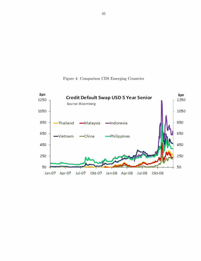
45
Figure 4: Comparison CDS Emerging Countries

46
Table 1: Results from posterior maximization
Prior distribution Prior mean Prior s.d. Posterior mode s.d.
�in;1 gamm 0.600 0.1000 0.4276 0.0675�in;2 beta 0.200 0.0500 0.1491 0.0396�in;3 gamm 0.250 0.0500 0.1643 0.0291�in;4 gamm 0.200 0.0500 0.1780 0.0453�in;5 gamm 0.050 0.0100 0.0347 0.0065 in;1 beta 0.500 0.0500 0.6279 0.0371 in;2 gamm 1.500 0.2000 1.3836 0.1783 in;4 gamm 0.200 0.0500 0.1856 0.0479
gY ssin norm 6.000 1.0000 5.2247 0.3691�in;1 beta 0.250 0.0500 0.2699 0.0565�in;2 gamm 0.250 0.0500 0.2088 0.0425�in;3 gamm 0.150 0.0500 0.1071 0.0283�in beta 0.500 0.0500 0.5299 0.0485�in beta 0.400 0.0500 0.3802 0.0318�in beta 0.500 0.1000 0.4950 0.1070rrin norm 2.000 0.5000 2.2032 0.4307� in beta 0.050 0.0300 0.0332 0.0247�in beta 0.050 0.0005 0.0500 0.0005

47
Figure 5: Indonesia Historical In�ation Graph
2000 2001 2002 2003 2004 2005 2006 2007 20082
0
2
4
6
8
10
12
14PIE_HOPIETAR_HOY_HO

48
Table 2: Results from posterior parameters (standard deviation of structural shocks)
Prior distribution Prior mean Prior s.d. Posterior mode s.d.
"gY
in invg 0.100 Inf 0.0459 0.0187"Yin invg 0.200 Inf 0.5166 0.0734"Zin invg 1.000 Inf 0.4610 0.1885"�in invg 0.500 Inf 1.4817 0.1846"Rin invg 0.200 0.0400 0.1855 0.0339"Rin�Rus invg 1.000 Inf 12.2522 1.4929eIin invg 0.500 0.0500 0.5371 0.0656"�
tar
in invg 0.250 0.0500 0.2487 0.0504"yin invg 0.300 Inf 0.1247 0.0423
"gZ
in invg 0.100 0.0010 0.0992 0.0050

49
Table 3: Results from posterior parameters (correlation of structural shocks)
Prior distribution Prior mean Prior s.d. Posterior mode s.d.
"Yin; "�in beta 0.100 0.0300 0.0971 0.0304
"yin; "gY
in beta 0.250 0.1000 0.2175 0.1038

50
Table 4: Root Mean Squared Errors
1 Q Ahead 4 Q Ahead 8 Q Ahead 12 Q Ahead
Output Gap IN yIN 0.516 0.655 0.717 0.644GDP Quarterly Growth at annual rates IN 4(YIN � YIN;�1) 2.34 1.87 1.28 1.12GDP Year-on-Year Growth IN YIN � YIN;�4 0.578 1.3 1.05 0.764GDP Y-o-Y Growth Potential IN 0.547 1.32 1.24 1.16CPI Year-on-Year In�ation IN �4IN 0.471 1.75 1.94 2.14Short-term Interest Rate (RS) IN rsIN 0.711 2 2.56 3.18

51
Figure 6: Domestic demand shock
10 20 30 400.05
0
0.05
0.1
0.15Y_HO
10 20 30 400.01
0
0.01
0.02
0.03PIE4_HO
10 20 30 400.02
0
0.02
0.04PIE_HO
10 20 30 400.02
0
0.02
0.04RS_HO
10 20 30 400.2
0.15
0.1
0.05
0LZ_HO
10 20 30 400.2
0.15
0.1
0.05
0REER_T_HO
10 20 30 400.2
0.1
0
0.1
0.2GROWTH4_HO
10 20 30 400.5
0
0.5
1GROWTH_HO
10 20 30 400.01
0
0.01
0.02
0.03RR_HO

52
Figure 7: Domestic price shock
10 20 30 400.2
0
0.2
0.4
0.6Y_HO
10 20 30 401
0.5
0
0.5PIE4_HO
10 20 30 402
1
0
1PIE_HO
10 20 30 401
0.5
0
0.5RS_HO
10 20 30 400
1
2
3LZ_HO
10 20 30 400
1
2
3REER_T_HO
10 20 30 400.1
0
0.1
0.2
0.3GROWTH4_HO
10 20 30 400.1
0
0.1
0.2
0.3GROWTH_HO
10 20 30 400.6
0.4
0.2
0
0.2RR_HO

53
Figure 8: Domestic interest rate shock
10 20 30 400.3
0.2
0.1
0
0.1Y_HO
10 20 30 400.2
0.1
0
0.1
0.2PIE4_HO
10 20 30 400.2
0.1
0
0.1
0.2PIE_HO
10 20 30 400.5
0
0.5RS_HO
10 20 30 401.5
1
0.5
0
0.5LZ_HO
10 20 30 401.5
1
0.5
0
0.5REER_T_HO
10 20 30 400.4
0.2
0
0.2
0.4GROWTH4_HO
10 20 30 400.6
0.4
0.2
0
0.2GROWTH_HO
10 20 30 400.2
0
0.2
0.4
0.6RR_HO

54
Figure 9: Domestic real exchange rate shock
10 20 30 400.1
0
0.1
0.2
0.3Y_HO
10 20 30 400.1
0
0.1
0.2
0.3PIE4_HO
10 20 30 400.2
0
0.2
0.4
0.6PIE_HO
10 20 30 400.2
0
0.2
0.4
0.6RS_HO
10 20 30 402
0
2
4
6LZ_HO
10 20 30 402
0
2
4
6REER_T_HO
10 20 30 400.2
0
0.2
0.4
0.6GROWTH4_HO
10 20 30 400.5
0
0.5
1GROWTH_HO
10 20 30 400.2
0
0.2
0.4
0.6RR_HO

55
Figure 10: Shock to the domestic target rate of in�ation
10 20 30 400.2
0.1
0
0.1
0.2Y_HO
10 20 30 400.4
0.3
0.2
0.1
0PIE4_HO
10 20 30 400.4
0.3
0.2
0.1
0PIE_HO
10 20 30 400.4
0.2
0
0.2
0.4RS_HO
10 20 30 401.5
1
0.5
0
0.5LZ_HO
10 20 30 401.5
1
0.5
0
0.5REER_T_HO
10 20 30 400.2
0.1
0
0.1
0.2GROWTH4_HO
10 20 30 400.4
0.2
0
0.2
0.4GROWTH_HO
10 20 30 400.2
0
0.2
0.4
0.6RR_HO

56
Figure 11: Demand shock in the US
10 20 30 400.2
0
0.2
0.4
0.6Y_US
10 20 30 400.02
0
0.02
0.04Y_JA
10 20 30 400.02
0
0.02
0.04
0.06Y_EU
10 20 30 400.02
0
0.02
0.04Y_HO
10 20 30 400.01
0
0.01
0.02
0.03PIE4_HO
10 20 30 400.05
0
0.05
0.1
0.15RS_HO
10 20 30 400.1
0
0.1
0.2
0.3LZ_HO
10 20 30 400.02
0
0.02
0.04GROWTH4_HO
10 20 30 400.02
0
0.02
0.04RR_HO

57
Figure 12: BLT shock in the US
10 20 30 400.1
0
0.1
0.2
0.3Y_US
10 20 30 400.02
0
0.02
0.04
0.06Y_JA
10 20 30 400.02
0
0.02
0.04
0.06Y_EU
10 20 30 400.02
0
0.02
0.04Y_HO
10 20 30 400.02
0
0.02
0.04
0.06PIE4_HO
10 20 30 400.05
0
0.05
0.1
0.15RS_HO
10 20 30 400.2
0
0.2
0.4
0.6LZ_HO
10 20 30 400.04
0.02
0
0.02
0.04GROWTH4_HO
10 20 30 400.05
0
0.05
0.1
0.15RR_HO