1

Geophysical Research Letters

Supporting Information for

Sibling earthquakes generated within a persistent rupture barrier on the Sunda megathrust under Simeulue Island

Paul M. Morgan1, Lujia Feng1, Aron J. Meltzner1,

Eric O. Lindsey1, Louisa L. H. Tsang1, and Emma M. Hill1,2

1Earth Observatory of Singapore, Nanyang Technological University, Singapore

2Asian School of the Environment, Nanyang Technological University, Singapore

Contents of this file

Text S1 and S2 Figures S1 to S11 Captions for Data Sets S1 to S4

Additional Supporting Information (Files uploaded separately)

Data Sets S1 to S4

Introduction

This supporting information documents further details on the data and modeling methods used to derive slip distributions for the 2002 MW 7.3 and 2008 MW 7.4 events, including Text S1 to S2 and additional figures from Figure S1 to Figure S11. It also provides data sets of the coral measurements and slip distributions for the 2002 and 2008 Simeulue events.

2

Text S1. Displacement calculation for the 2008 MW 7.4 earthquake Here we detail how we used a planar correction based on the GPS sites to convert the

relative values of our interferogram to absolute values. We used ALOS-1 PALSAR acquisitions on Feb. 16, 2008 and Jul. 3, 2008 (Path 500, Frames 30-40) to generate an interferogram, which records a relative displacement field in the line of sight (LOS) direction. There is a small ~30 mm offset in the LOS deformation between the two ALOS-1 frames combined to form the interferogram, likely an artifact resulting from the alignment procedure applied to the northern frame, which was acquired mostly over the ocean and therefore has only a small proportion of valid data. We corrected this by adding a constant shift to the northern scene before combining the data into one relative displacement field. As this relative displacement field had no zero-deformation control points, we had to use GPS displacements to correct the relative LOS of the InSAR to absolute LOS displacements. The GPS displacements we used cover the same time span as the InSAR acquisition, and they were calculated based on a model fit to the raw time series [Feng et al., 2015]. Using a model instead of raw data is required due to a data gap at site LEWK that spans from two months after the earthquake until after the second InSAR acquisition. We not only used GPS displacements to correct the InSAR relative LOS displacements to absolute values, but also used them directly in our inversion.

To correct the InSAR from relative to absolute LOS, the simplest way is to calculate the difference between the relative LOS values from InSAR and the absolute LOS values from GPS at GPS site locations. In an ideal case, one difference value could be subtracted across the entire scene to correct the interferogram, so that the displacements of the two measurements match. However, the interferogram has orbital errors and atmospheric noise. These extra errors are usually assumed to be distributed as a plane across the entire scene. Thus, we used a plane instead of one single value to subtract from the interferogram. However, Simeulue had only two GPS stations, which is not enough to constrain a plane. Hence we assumed a plane that matched both stations and aligned its steepest gradient parallel to the line between the two stations. The slope of this planar correction is on the order of 25mm over the 90km baseline between the two sites.

We tested the effect of our assumption that the steepest gradient of the planar correction lies parallel to the direction between the GPS points, by adding extra planar corrections. We introduced a gradient of the same magnitude to the perpendicular orientation (both positive and negative slopes) and re-did the modeling. We found that the resulting slip distributions are barely distinguishable, indicating that uncertainties in the estimation of the ramp are not likely to significantly affect our results. The corrected final InSAR displacement field was later downsampled to 371 evenly distributed points, spaced 2 km apart, and used for inversion.

3

Text S2. Moment estimates from the geodetic models Here we compare the moment estimates from our geodetic models to moment estimates that are seismically constrained. We estimate a magnitude range of Mw~7.34-7.43 (with shear moduli of 30-40 GPa) for the 2008 event, and Mw~7.08-7.16 for the 2002 event. These estimates are based on slip estimated for patches only within the contours shown in Figures 2 and 3. These compare with values of 7.4 (2008) and 7.3 (2002) as estimated by Duputel et al., [2013]. Our estimated Mw for the 2002 event is therefore a little low. However, we note that absolute values for slip are notoriously difficult to estimate from sparse geodetic data, especially in the presence of slip constraints in the inversion. While we can change the maximum slip by varying the Laplacian smoothing weight or by applying additional constraints, we believe the location of the slip to be robust.

4

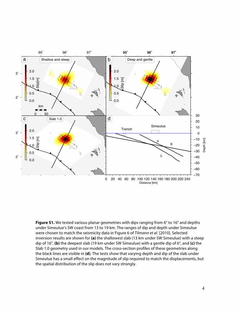
Figure S1. We tested various planar geometries with dips ranging from 6° to 16° and depths under Simeulue’s SW coast from 13 to 19 km. The ranges of dip and depth under Simeulue were chosen to match the seismicity data in Figure 6 of Tilmann et al. [2010]. Selected inversion results are shown for (a) the shallowest slab (13 km under SW Simeulue) with a steep dip of 16°, (b) the deepest slab (19 km under SW Simeulue) with a gentle dip of 6°, and (c) the Slab 1.0 geometry used in our models. The cross-section profiles of these geometries along the black lines are visible in (d). The tests show that varying depth and dip of the slab under Simeulue has a small effect on the magnitude of slip required to match the displacements, but the spatial distribution of the slip does not vary strongly.

95˚ 96˚ 97˚

2˚

3˚

0.0

0.5

1.0

1.5

2.0

Slip

[m]

a Shallow and steep

0 50

km

2˚

3˚

0.0

0.5

1.0

1.5

2.0

Slip

[m]

c Slab 1.0

95˚ 96˚ 97˚95˚ 96˚ 97˚

0.0

0.5

1.0

1.5

2.0

Slip

[m]

b Deep and gentle

−70−60−50−40−30−20−10

0102030

0 20 40 60 80 100 120 140 160 180 200 220 240

d

TrenchSimeulue

AB

C

Distance [km]

Dep

th [k

m]

5

Figure S2. We tested the effect of varying relative weightings between the GPS and InSAR data on our inversion results for the 2008 MW 7.4 event. The uncertainty for InSAR displacements was set uniformly as 1 m, while the uncertainty for GPS displacements was on the order of 5 mm. The preferred weighting is GPS weighted at 1 and the InSAR weighted at 0.1. The results from joint inversion are consistent for different relative weightings. The position of the slip patch under Simeulue does not change significantly over this shift of two orders of magnitude in relative weighting between the InSAR and GPS displacements.

95˚ 96˚ 97˚

2˚

3˚

0

1

2

3

Slip

[m]

a GPS 10 times more weight

2˚

3˚

0

1

2

3

Slip

[m]

b Preferred weighting

95˚ 96˚ 97˚

2˚

3˚

0

1

2

3

Slip

[m]

c InSAR 10 times more weight

0 50

km

6

Figure S3. We tested the effect of varying smoothing on our inversion results for the 2008 MW 7.4 event. (a), (b), and (d) The best-fit models for selected values of the smoothing parameter κ. (c) The tradeoff curve between roughness and data misfit. Model (b) represents our preferred model with κ = 2000 (red star).

95˚ 96˚ 97˚

2˚

3˚

0.00.51.01.52.0

Slip

[m]

a κ = 5000

95˚ 96˚ 97˚

0.00.51.01.52.0

Slip

[m]

b κ = 2000

0.00.51.01.52.0

Slip

[m]

d κ = 750

0.00

0.02

0.04

0.06

0.08

0.10

0.0 0.5 1.0

c

κ = 750

κ = 5000

κ = 2000

Roughness [mm/km2]

WR

MS

[m]

7

Figure S4. We conducted a checkerboard test on the spatial resolution of the InSAR and GPS data used for the 2008 event. (a) Synthetic input slip distribution with alternating 1 or 0 m of thrust motion. (b) Output best-fit slip results using the same relative weighting as used for the preferred 2008 slip model. The test shows that slip under Simeulue can be well resolved by the available data.

95Ý 95.5Ý 96Ý 96.5Ý ��Ý

�Ý

���Ý

�Ý

95Ý 95.5Ý 96Ý 96.5Ý ��Ý

�Ý

���Ý

�Ý

0 50km

0.0 0.5 1.0 1.5

Slip [m]

a 2008 Mw 7.4

�Ý

���Ý

�Ý

�Ý

���Ý

�Ý

b InSAR and GPS

8

Figure S5. Coral-based observations and model estimates of vertical displacement for the 2008 earthquake. Raw vertical displacement measurements for 2008 are not as spatially coherent as those for the 2002 event (Figure 3a). At all coral sites, the measured displacements, displayed as large circles and vectors with 2σ error ellipses (width not meaningful), span from 2005–2007 to 2008–2009 (Data Set S2), and thus contain deformation signals from postseismic processes following the 2004 and 2005 earthquakes, along with deformation from 2008 coseismic and postseismic processes. Where two independent measurements exist for the same site, we plot the weighted average. These spatiotemporally complex signals do not allow for an inversion of the coral data as we conducted for the 2002 event. The discrepancies between the observations and our model predictions are largest on the western southwest coast of Simeulue (near sites USL, BHN, and ULB), where the model predicts much greater uplift than observed. Because the coral observations at these three sites represent the net change between 2005/2006 and 2008/2009, this systematic discrepancy could be explained if postseismic subsidence following the 2004/2005 earthquakes was particularly large at those sites and cancelled out some of the coseismic uplift in 2008. In addition, any systematic misfits between the coral data on the east and west sides of the island could be due to an imperfect planar correction in the interferogram. The exact causes of the misfits are unknown, but these misfits should not make a significant difference in the coseismic model (Figure 2b) or the conclusions of this study.

95.5Ý 96Ý 96.5Ý ��Ý

���Ý

�Ý

��������FRUDO�GDWD)RUZDUG�PRGHO

����

0

���200

300

400

500

9HUWLFDO�'

LVSODFHP

HQW�>PP@

0 �� 20

NP����PP&RUDO�GDWD

USL

BHN

ULB

9

Figure S6. Model fits to the data recording the 2008 event. (a) The unwrapped, evenly distributed LOS displacement points extracted from the interferogram, and the GPS displacements used in the inversion. (b) The displacements predicted by our preferred model. (c) The residuals, model value – data value, for each point used in the inversion. Note that the GPS residuals are essentially zero.

���Ý

�Ý

20 mm

GPS data

LEWK

BSIM

0

100

200

300

400

500

600

Da

ta L

OS

dis

pla

ce

me

nt

(mm

)a 2008 Mw 7.4Data

���Ý

�Ý

20 mm

Model GPS0

100

200

300

400

500

600

Mo

de

l L

OS

dis

pla

ce

me

nt

(mm

)b Model

LOS direction

95.5Ý 96Ý 96.5Ý ��Ý

���Ý

�Ý

20 mm

Residual GPS

�����

0

10

20

30

40

50

5HVLGXDO��0RGHO�ï�GDWD��PP�c Residual

10

Figure S7. Flow chart that summarizes the forward modeling steps that provide the area for the inversion of the 2002 earthquake. In this figure, we define a “fault patch” as any single 10 km by 10 km element making up the fault interface, and we define a “slip rectangle” as a rectangular-shaped contiguous grouping of fault patches, up to 90 km along strike and 70 km along dip.

Step 1

Step 2

Step 3

Step 4

Step 5

Example locations

Make a set of uniform slip rectangles

Run a suite of forward models with each slip rectangle everywhere

Find the lowest misfit “sweet spot”

Compile the set of “sweet spot” rectangles for rectangles

of every size

Use the “sweet spot” locations to define inversion constraints

We choose a set of possible uniform slip rectangles to represent the 2002 rupture. The size of the rectangles ranges from 10 to 90 km along strike and 10 to 70 km along dip. The slip value for each slip rectangle is scaled by the area to fit the moment of the 2002 rupture. We show here 10 examples out of the total 63 slip rectangles considered.

We shift each slip rectangle across the extent of our fault geometry every 10 km along strike or dip. For each slip rectangle at each location, we calculate the uplift predictions from the slip rectangle (blue vectors) and compare them to the actual measurements (red vectors).

For each slip rectangle at each location, we calculate the misfit between the synthetic forward model predictions and the uplift measurements. For each slip rectangle, we then compare the misfit values spatially to find the “sweet spot” where the slip rectangle produces displacements that fit the data best.

We compile the set of best-fit locations, one location for each size of slip rectangle, and we color each slip rectangle according to its rms misfit. To constrain the area, we consid-er the locations, and not rms misfits of these best-fit slip rectangles.

The best fit, sweet spot slip rectangleA poor fit

We color each fault patch by the number of “sweet spot” slip rectangles that include this particular patch. We constrain the area for the inversion to be within the black dashed line, which encloses nearly all of the colored patches. The preferred slip model (green contours) is contained within the black dashed line.

How we use a suite of forward models to constrain the inversion for the 2002 MW 7.3 earthquake

0 1 2 3 4 5 6 7

forward slip [m]

����Ý ��Ý ����Ý ��Ý ����Ý ��Ý ����Ý���Ý

�Ý

���Ý

�Ý

���Ý

�Ý

0 10 20 30 40

Number of Best fit solutions including this patch

0.02 0.04 0.06 0.08 0.10

rms outline of the best fitting location

0.05 0.10 0.15rms

rms is 0.0463028���� 0 150 300

residual [mm]

50 mm

Forward predictions

���� 0 150 300

residual [mm]

rms is 0.166774

50 mm

Forward predictions

50 mm

Input data

11

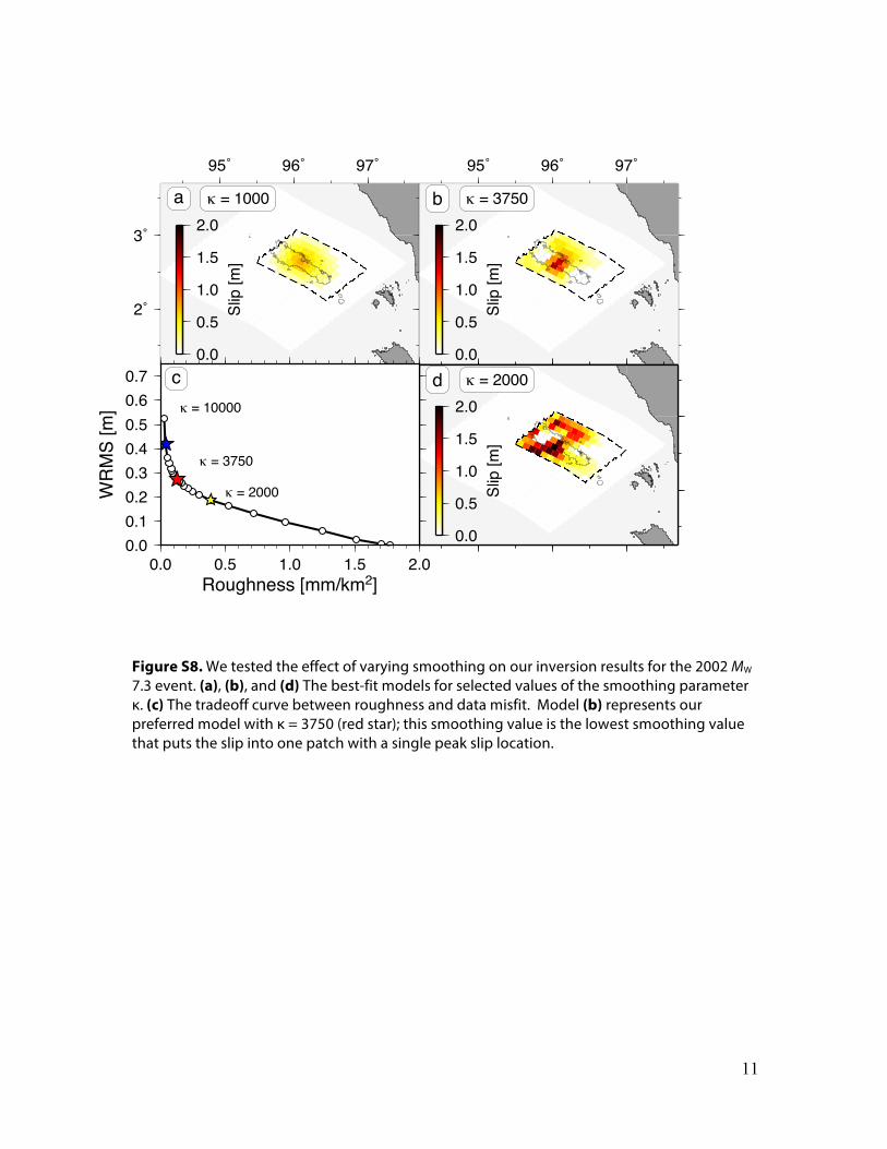
Figure S8. We tested the effect of varying smoothing on our inversion results for the 2002 MW 7.3 event. (a), (b), and (d) The best-fit models for selected values of the smoothing parameter κ. (c) The tradeoff curve between roughness and data misfit. Model (b) represents our preferred model with κ = 3750 (red star); this smoothing value is the lowest smoothing value that puts the slip into one patch with a single peak slip location.

95˚ 96˚ 97˚

2˚

3˚

0.0

0.5

1.0

1.5

2.0Sl

ip [m

]

a κ = 1000

95˚ 96˚ 97˚

0.0

0.5

1.0

1.5

2.0

Slip

[m]

b κ = 3750

0.0

0.5

1.0

1.5

2.0

Slip

[m]

d κ = 2000

0.00.10.20.30.40.50.60.7

0.0 0.5 1.0 1.5 2.0

c

κ = 2000

κ = 10000

κ = 3750

Roughness [mm/km2]

WR

MS

[m]

12

Figure S9. We conducted a checkerboard test on the spatial resolution of the coral data used for the 2002 event. (a) Synthetic input slip distribution with alternating 1 or 0 m of thrust motion. (b) Output best-fit slip results constrained within the same dashed box as we used in our final solution for the 2002 event. The test shows that the few coral sites may be capable of resolving the location of slip on the fault interface under Simeulue.

95.5Ý 96Ý 96.5Ý ��Ý

���Ý

�Ý

95.5Ý 96Ý 96.5Ý ��Ý

���Ý

�Ý

0 50km

0.0 0.5 1.0 1.5

Slip [m]

a 2002 Mw 7.3

���Ý

�Ý

���Ý

�Ýb Coral only

13

Figure S10. We compared our coral uplift measurements for the 2002 event with the predictions from the one published slip model (color patches) [DeShon et al., 2005]. The DeShon et al. [2005] model overpredicts uplift at all coral sites, and it fails to predict the uplift gradient between the larger uplift recorded at the central Simeulue sites and the negligible uplift recorded at the western sites. The large misfit between our coral data and the predictions from the DeShon model motivated us to derive our slip distribution based solely upon the coral uplift data. For comparison, the 0.5 m contour of our preferred slip model is shown as a green line.

95.5Ý 96Ý 96.5Ý ��Ý

���Ý

�Ý

���Ý

DeShon model predictions

Coral measurements

0

1

2

3

4

5

6

7

Slip

[m]

100 mm

Displacement

0 10 20 30

km

14

Figure S11. A comparison of the coral observations of uplift in 2002 with a uniformly scaled forward model of uplift in 2008. Only sites discussed here are labeled. We used least squares to calculate the scaling factor that would result in the best fit of the scaled 2008 slip distribution to 2002 coral data, at the 2002 observation sites. Our estimated scaling factor is 0.3. The fit is not bad, but the uplifts are overestimated on the western side of the island, notably at sites BHN and LWK, and underestimated at sites in the southeast, notably ULB and BUN. This suggests that the peak slip of the 2008 event was to the west of the peak slip for the 2002 event. Though both events may have ruptured the same asperity, this offset in the peak slip is what leads us to refer to the events not as “twins” or repeating earthquakes, but as “siblings”.

95.5Ý 96Ý 96.5Ý ��Ý

���Ý

�Ý

���Ý

100 mm

2008 scaled model predicted

100 mm

2002 data

0 10 20 30

km

BHN

ULB

LWK

BUN

15

Data Set S1.

Coral vertical displacements associated with the 2002 MW 7.3 rupture. Coral microatolls at the sites listed in Data Set S1 experienced a diedown around the beginning of 2004, presumably in Jan or Feb 2004, at the time of the first extreme negative sea level anomalies following the Nov 2002 earthquake [Meltzner et al., 2010]. (Some sites experienced an initial diedown at the beginning of 2003, followed by a lower diedown at the beginning of 2004.) The uplift (or subsidence) estimates in Data Set S1 are based on the amplitude of the early 2004 diedown at each site, with corrections for the difference in the lowest water levels before and after the 2002 earthquake, as well as for interseismic deformation, extrapolated from pre-1997 rates. Considering these corrections [which are discussed further by Meltzner et al., 2010], the uplifts (or subsidence) calculated in Data Set S1 effectively represent the net vertical deformation from the moment of the 2002 earthquake until the time of the lowest water level in Jan 2004. Note that the uplift estimate at BHN-A is based on a site survey, whereas all other estimates are based on coral slabs excavated from the site [Meltzner et al., 2010, 2012, 2015].

The errors are conservatively treated as uncorrelated, and are largely derived from uncertainties in the tidal model and in the sea level anomalies and are reduced when the highest level of survival (HLS) is measured on an increasingly large set of corals (and averaged) and/or when the number of water level measurements is increased.

Data Set S2.

Coral vertical displacements associated with the 2008 MW 7.4 rupture. Multiple visits were made to each site listed in Data Set S2a in the months to years following the 2004 and 2005 earthquakes. During each visit, the corals’ pre-2004 or pre-2005 highest level of growth was surveyed relative to instantaneous water level. We corrected for (1) the tidal elevation at the time of the survey, (2) the sea level anomaly at the time of the survey, and (3) the inverted barometer effect at the time of the survey; this allowed us to place all surveyed coral elevations (from the various visits) into a common vertical reference frame. (The surveys and corrections are discussed further by Meltzner et al., 2010.) If there had been no tectonic deformation, we would expect the coral elevations to have been the same (within error) on every visit; any difference over time in the coral elevations (beyond error) is inferred to reflect net vertical deformation at the site between the first visit (time1) and the second visit (time2). For sites that appear in both Data Set S2a and Data Set S2b, the two estimates of vertical change at the site should be considered as independent of one another. The sites listed in Data Set S2b experienced a coral diedown in early to mid-2008, presumably in Jun 2008, at the time of the first extreme negative sea level anomalies following the Feb 2008 earthquake [Meltzner et al., 2010]. The uplift estimates in Data Set S2b are based on the amplitude of the coral diedown following the 2008 earthquake at each site, with a correction for the difference in the lowest water levels before and after the 2008 earthquake. For sites NOT uplifted in 2005 (i.e., in western Simeulue), the lowest water level between the 2004 and 2008 earthquakes occurred in Mar 2005, weeks before the 2005 earthquake; for sites uplifted in 2005 (i.e., in eastern Simeulue), the lowest water level between the 2005 and 2008 earthquakes occurred in Sep 2006. The uplifts calculated in Data Set S2b, therefore, represent the net uplift between the preceding lowest water level (Mar 2005 or Sep 2006) and the lowest water level in Jun 2008. See Meltzner et al. [2010, 2012, 2015] for further discussion. For sites that appear in both Data Set S2a and Data Set S2b, the two estimates of vertical change at the site should be considered as independent of one another.

16

Data Set S3.

Slip distribution for our preferred model of the 2002 MW 7.3 rupture. See file for explanation of columns.

Data Set S4.

Slip distribution for our preferred model of the 2008 MW 7.4 rupture. See file for explanation of columns.