adele cutler utah state university · adele cutler . utah state university . random forests ....
TRANSCRIPT

Adele Cutler
Utah State University
Random Forests

Random Forests

Leo Breiman January 27, 1928 - July 5, 2005

Outline
• What are random forests?
• Background • New features since Breiman (2001)
– Proximities •Imputing missing values •Clustering
– Unequal class sizes – Local variable importance – Visualization

Outline
• What are random forests?
• Background • New features since Breiman (2001)
– Proximities •Imputing missing values •Clustering
– Unequal class sizes – Local variable importance – Visualization

Drawbacks of a classification tree: • Accuracy: state-of-the-art methods have
much lower error rates than a single classification tree.
• Instability: if you change the data a little, the tree picture can change a lot, so the interpretation is built on shifting sands.
Today, we can do better!
Random Forests

What are Random Forests? Grow a forest of trees: • each tree is grown on an independent
bootstrap sample from the training data.
• independently, for each node of each tree, find the best split on m randomly selected variables.
• grow deep trees. Get the prediction for a new case by voting (averaging) the predictions from all the trees.

Properties of Random Forests
1. Accurate. – In independent tests on collections of data
sets it’s neck-and-neck with the best known machine learning methods (eg SVMs).
2. Fast.
– With 100 variables, 100 trees in a forest can be grown in the same time as growing 3 single CART trees.
3. Do not overfit as we add more trees.

4. Handles – thousands of variables – many-valued categoricals – extensive missing values – badly unbalanced data sets.
5. Gives an internal estimate of test set error as
trees are added to the ensemble. 6. Gives variable importance measures and
proximities for visualization/clustering. Leo: gives a wealth of scientifically important
insights!

Outline
• What are random forests?
• Background • New features since Breiman (2001)
– Proximities •Imputing missing values •Clustering
– Unequal class sizes – Local variable importance – Visualization

Random Forests
|protein< 45.43
bilirubin>=1.8
alkphos< 149
albumin< 3.9
albumin< 2.75
varices< 1.5
bilirubin>=1.8021/0
09/0
10/4
10/7
03/0
04/0
10/7
12/98
How do they work?

Random Forests
|protein< 45.43
bilirubin>=1.8
alkphos< 149
albumin< 3.9
albumin< 2.75
varices< 1.5
bilirubin>=1.8021/0
09/0
10/4
10/7
03/0
04/0
10/7
12/98
|protein< 45
alkphos< 171
fatigue< 1.5
bilirubin>=3.65
bilirubin< 0.5
sgot< 29protein< 66.9
age< 50
021/1
10/2
10/8
03/1
02/0
05/0
10/2
10/20
11/89
How do they work?

Random Forests
|protein< 45
alkphos< 171
fatigue< 1.5
bilirubin>=3.65
bilirubin< 0.5
sgot< 29protein< 66.9
age< 50
021/1
10/2
10/8
03/1
02/0
05/0
10/2
10/20
11/89
|protein< 45.43
bilirubin>=1.8
alkphos< 149
albumin< 3.9
albumin< 2.75
varices< 1.5
bilirubin>=1.8021/0
09/0
10/4
10/7
03/0
04/0
10/7
12/98
|protein< 45.43
prog>=1.5
fatigue< 1.5 sgot>=123.8
025/0
10/2
02/0
10/11
11/114
How do they work?

|protein< 46.5
albumin< 3.9
alkphos< 191
bilirubin< 0.65
alkphos< 71.5 varices< 1.5
firm>=1.5
021/1
10/2
10/7
02/0
11/11
02/0
10/6
10/102
Random Forests
|protein< 45
alkphos< 171
fatigue< 1.5
bilirubin>=3.65
bilirubin< 0.5
sgot< 29protein< 66.9
age< 50
021/1
10/2
10/8
03/1
02/0
05/0
10/2
10/20
11/89
|protein< 45.43
prog>=1.5
fatigue< 1.5 sgot>=123.8
025/0
10/2
02/0
10/11
11/114
How do they work?
|protein< 45.43
bilirubin>=1.8
alkphos< 149
albumin< 3.9
albumin< 2.75
varices< 1.5
bilirubin>=1.8021/0
09/0
10/4
10/7
03/0
04/0
10/7
12/98

Random Forests
|protein< 45
alkphos< 171
fatigue< 1.5
bilirubin>=3.65
bilirubin< 0.5
sgot< 29protein< 66.9
age< 50
021/1
10/2
10/8
03/1
02/0
05/0
10/2
10/20
11/89
|protein< 45.43
bilirubin>=1.8
alkphos< 149
albumin< 3.9
albumin< 2.75
varices< 1.5
bilirubin>=1.8021/0
09/0
10/4
10/7
03/0
04/0
10/7
12/98
|protein< 45.43
prog>=1.5
fatigue< 1.5 sgot>=123.8
025/0
10/2
02/0
10/11
11/114
|protein< 46.5
albumin< 3.9
alkphos< 191
bilirubin< 0.65
alkphos< 71.5 varices< 1.5
firm>=1.5
021/1
10/2
10/7
02/0
11/11
02/0
10/6
10/102
|protein< 50.5
albumin< 3.8
alkphos< 171
fatigue< 1.5
bilirubin< 0.65
alkphos< 71.5
025/0
10/2
10/5
10/8
03/1
10/9
10/102
How do they work?

Random Forests
|protein< 45
alkphos< 171
fatigue< 1.5
bilirubin>=3.65
bilirubin< 0.5
sgot< 29protein< 66.9
age< 50
021/1
10/2
10/8
03/1
02/0
05/0
10/2
10/20
11/89
|protein< 45.43
bilirubin>=1.8
alkphos< 149
albumin< 3.9
albumin< 2.75
varices< 1.5
bilirubin>=1.8021/0
09/0
10/4
10/7
03/0
04/0
10/7
12/98
|protein< 45.43
prog>=1.5
fatigue< 1.5 sgot>=123.8
025/0
10/2
02/0
10/11
11/114
|protein< 46.5
albumin< 3.9
alkphos< 191
bilirubin< 0.65
alkphos< 71.5 varices< 1.5
firm>=1.5
021/1
10/2
10/7
02/0
11/11
02/0
10/6
10/102
|protein< 50.5
albumin< 3.8
alkphos< 171
fatigue< 1.5
bilirubin< 0.65
alkphos< 71.5
025/0
10/2
10/5
10/8
03/1
10/9
10/102
|protein< 45.43
sgot>=62
prog>=1.5
bilirubin>=3.65
019/1
04/1
10/7
03/0
14/116
Leo: Looking at the trees is not going to tell us very much.
How do they work?

Illustration - Hepatitis protein and alkaline phosphate
|protein< 45.43
protein>=26
alkphos< 171
protein< 38.59alkphos< 129.40
19/0 04/0
11/2
11/4
10/3
17/114

Illustration - Hepatitis protein and alkaline phosphate
|protein< 45.43
protein>=26
alkphos< 171
protein< 38.59alkphos< 129.40
19/0 04/0
11/2
11/4
10/3
17/110 20 40 60 80 100
050
100
150
200
250
300
protein
alka
line
phos
phat
e
1
1
1
1
1
1
0
11 11
1
1
1
11
1
11
1
1
1
1
11
11
1
11
0
0
1
1
10
1
1
1
1
1
11
1111
1
1
1
11
1
1
1
11
1
1 1
1
1
1
1
1
11
0
1
11
0
11
1
1
0
1
111
1
1
1
1
1
0
0
0
1
1
0
1
10
1
1
1
01
0
1
1
1
0 1
0 11
0
1
0
11
1
1
1
1
0
10
1
11
11
1
0
101
0
1
1
0
1
1
1
0
1
1
0 1
0
0
10
0
1
10 1
11
0
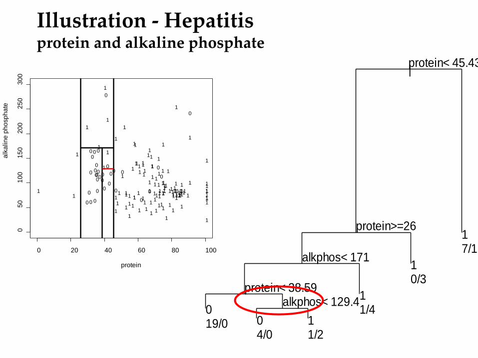

0.0 0.2 0.4 0.6 0.8 1.0
0.0
0.2
0.4
0.6
0.8
1.0
0
1
1
0
1
1
0
0
1
0
0
1
1
0
0
1
1
1
00
1
0
1
1
0
1
0
1
0
0 0
1
1
1
1
1
0
0
1
1
0
1
0
01
1
1
0
1
0
0
1
0
0
0
1
0
1
110
00
1
1
0
1
1
0
10
0
1
1
0
0
1
0
0
1
0
1
1
0
1
0
0
0
0
1
0
0
0
1
0
0
0
1
1
0
0
0
0
1
11
1
0
00
0
0
11
0 0
1
0
1
0
1
1
1
0
0
1
0
0
1
0
1
1
1
10
1
1
0
1
1
1
00
1
1
0
11
11
00
0
0
0
1 1
0
0
0
0
0
0
11 1
0
1
0
1
0
0
1
0
0
01
0
111
1
10
1
0
0
10
0
1
1
0
1
1
0
1
0
0
1
0
1
1
1
0
11
0
1
0
0
1
11
0
1
1
0
0
0
1
0
1
0
1
0
1
0
0
1
1
1
1
00
0
0
1
0
0
11
0
0
11
0
0
1
1
1
1
1
0 1
01
0
1
1
0
1
0
11
0
0
1
0
1
0
0
1
1
0
1
1
1
1
0
1
0
0
0
1
1
1
1
1
0
1
0
0
11
0
1
1
1
0
1
1
1
1
0
0
0
1
11
0
0
1
1
1
0
0
1
1
0 00
1
0
0
1
0
00
1
1
1
0
10
00
1
1
0
0
0
10
0
1 1
1
1
0
0
0
1
1
1
00
1
1
0
0
1
1
0 0
1
0
0
0
1
0
0
1
1
00 0
1
1 1
1
00
1
0
0
00
1
0
1
1
0
0
0
0
0
100
0
0
1
00
0
1
1
0
0 1
000
0
10
1
1
1
0
1
1
1
0
0
1
10
11
1
0
1
0
1
1
1
1
10
0
0
1
0
1
0
1
1
10
0
0
1
1
1
0
1
1
1
0
0
0
1
0
11
0
1
0
0
0
00
1
0
10
1
0
1 1
0
1
1
0
1
0
1
1
0
0
0
1
0
0
0
0
0
1
Hard for a single tree:

0.2 0.4 0.6 0.8 1.0
0.2
0.4
0.6
0.8
1.0
Single Tree:

0.2 0.4 0.6 0.8 1.0
0.2
0.4
0.6
0.8
1.0
25 Averaged Trees:

0.2 0.4 0.6 0.8 1.0
0.2
0.4
0.6
0.8
1.0
25 Voted Trees:

Data and Underlying Function
-3 -2 -1 0 1 2 3
-1.0
-0.5
0.0
0.5
1.0

Single Regression Tree (all data)
-3 -2 -1 0 1 2 3
-1.0
-0.5
0.0
0.5
1.0

10 Regression Trees (fit to boostrap samples)
-3 -2 -1 0 1 2 3
-1.0
-0.5
0.0
0.5
1.0

Average of 100 Regression Trees (fit to bootstrap samples)
-3 -2 -1 0 1 2 3
-1.0
-0.5
0.0
0.5
1.0

Useful by-products of Random Forests
Bootstrapping → out-of-bag data → • Estimated error rate • Variable importance
Trees → proximities → • Missing value fill-in • Outlier detection • Illuminating pictures of the data
– Clusters – Structure – Outliers
Leo: We use every bit of the pig except its squeal

Out-of-bag Data
Think about a single tree from a Forest: • The tree is grown on a bootstrap sample
(“the bag”). • The remaining data are said to be “out-of-
bag” (about one-third of the cases). • The out-of-bag data serve as a test set for this
tree. Out-of-bag data give • Estimated error rate • Variable importance

The out-of-bag Error Rate Think of a single case in the training set: • It will be out-of-bag in about 1/3 of the trees. • Predict its class for each of these trees. • Its RF prediction is the most common
predicted class. If we fit 1000 trees, and a case is out-of-bag in 339 of
them, of which 303 say “class 1” 36 say “class 2” The out-of-bag error rate is the error rate of the RF predictor (can be done for each class).
The RF prediction is “1”.

Illustration – Satellite Data
• 4435 cases, 36 variables. • Test set: 2000 cases.
0 20 40 60 80 100
010
2030
40
Error rates, oob and test, sate
number of trees
error
%
oob error %test set error %

Variable Importance
For variable j, look at the out-of-bag data for each tree:
• randomly permute the values of variable j, holding the other variables fixed.
• pass these permuted data down the tree, save the classes.
Importance for variable j is error rate when _ out-of-bag variable j is permuted error rate where the error rates are averaged over the out-
of-bag data, then over the trees.

Case Study – Invasive Plants
Data courtesy of Richard Cutler, Tom Edwards 8251 cases, 30 variables, 2 classes:
– Absent (2204 cases) – Present (6047 cases)

Illustration: Invasive Plants Distance to Road relha
T-min-d

Outline
• What are random forests?
• Background • New features since Breiman (2001)
– Proximities •Imputing missing values •Clustering
– Unequal class sizes – Local variable importance – Visualization

Proximities
Proximity of two observations is the proportion of the time that they end up in the same node. The proximities don’t just measure similarity of the variables. They take into account the importance of the variables. •Two observations that have quite different values on the variables might have large proximity if they differ only on variables that are not important.
•Two observations that have quite similar values of the variables might have small proximity if they differ on inputs that are important.
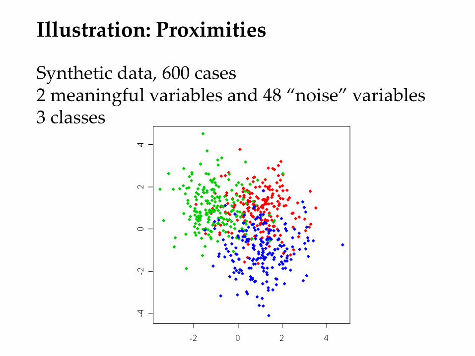
Illustration: Proximities
Synthetic data, 600 cases 2 meaningful variables and 48 “noise” variables 3 classes

Illustration: Proximities

Proximities
Proximity of two observations is the proportion of the time that they end up in the same node. Originally, we used all the data (in bag and out-of-bag). But we found that the proximities overfit the data…

Illustration: Proximities

Illustration: Proximities

Proximities
Two modifications : 1. Out-of-bag. Proximity of two observations is
the proportion of the time that they end up in the same node when they are both out-of-bag.
2. In and out. When observation i is out-of-bag, pass it down the tree and increment its proximity to all in-bag observations that end up in the same terminal node

Data 1

Data 2

Data 3

Nearest-neighbor classifiers from proximities
% error Data 1 Data 2 Data 3
Random Forests 64 23 4.7
Original 0 7 2.0
Out-of-bag 67 23 4.5
In and out 66 20 3.7

Nearest-neighbor classifiers from proximities
% Disagreement Compared to RF
Data 1 Data 2 Data 3
Original 64 16 3.0
Out-of-bag 48 5 0.5
In and out 15 3 1.0

Imputing Missing Values
Fast way: replace missing values for a given variable using the median of the non-missing values (or the most frequent, if categorical)
Better way (using proximities): 1. Start with the fast way. 2. Get proximities. 3. Replace missing values in case n by a weighted
average of non-missing values, with weights proportional to the proximity between case n and the cases with the non-missing values.
Repeat steps 2 and 3 a few times (5 or 6).

Outline
• What are random forests?
• Background • New features since Breiman (2001)
– Proximities •Imputing missing values •Clustering
– Unequal class sizes – Local variable importance – Visualization

Learning from Unbalanced Data
Increasingly often, data sets are occurring where the class of interest has a population that is a small fraction of the total population.
For such unbalanced data, a classifier can
achieve great accuracy by classifying almost all cases into the majority class!
RF weights the classes to get similar error rates
for each class.

Case Study – Invasive Plants
Data courtesy of Richard Cutler, Tom Edwards 8251 cases, 30 variables, 2 classes:
– Absent (2204 cases) – Present (6047 cases)
The 3 most important variables are Variable 1: distance to road Variable 12: relha Variable 23: t-min-d

Initial run, m=5, equal weights
Error rate = 6% Out-of-bag confusion matrix
Absent Present
Called absent 1921 213
Called present 283 5834
Total 2204 6047 Error rate 12.8% 3.5%

Second run, m=5, weight 3 to 1
Error rate = 8.7% Out-of-bag confusion matrix
Absent Present
Called absent 2099 614
Called present 105 5433
Total 2204 6047 Error rate 4.8% 10.2%

Third run, m=5, weight 2 to 1
Error rate = 7.0% Out-of-bag confusion matrix
Absent Present
Called absent 2051 421
Called present 153 5626
Total 2204 6047 Error rate 7.0% 7.0%

Important Variables
30 variables in all Weighted: Top 3 variables are 1, 12, 23 Variable 1: distance to road Variable 12: relha Variable 23: t-min-d Unweighted: Top 3 variables are 23, 1, 17 Variable 17: t-ave-d
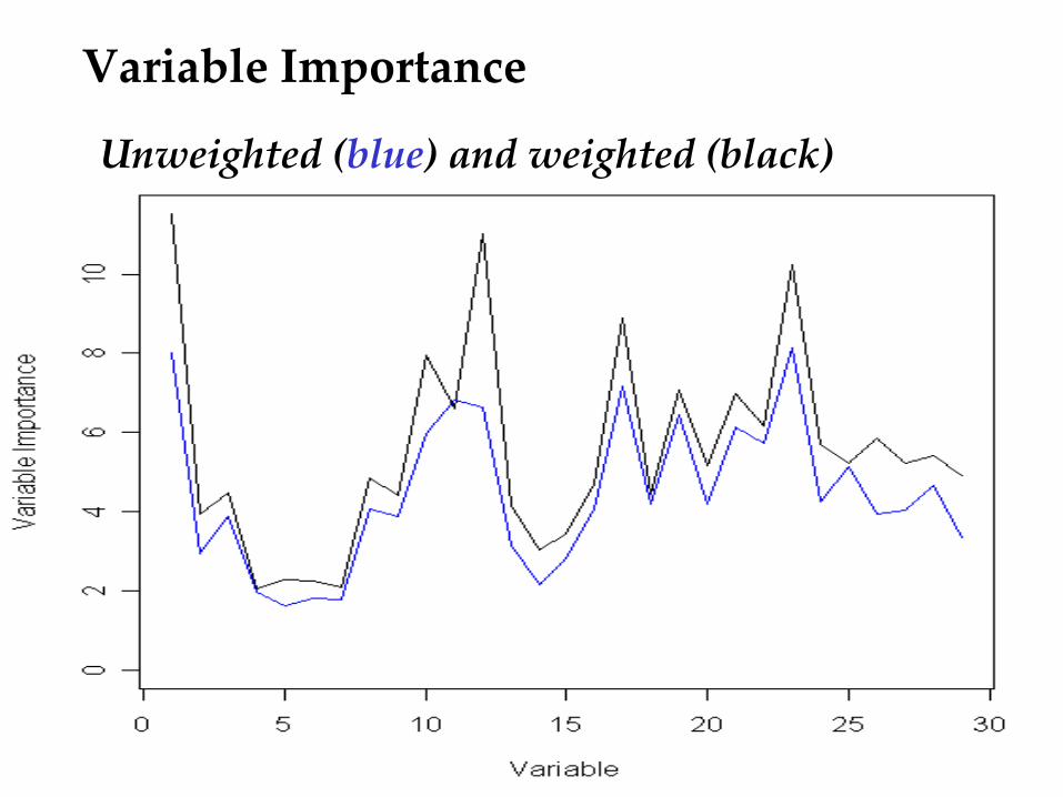
Variable Importance
Unweighted (blue) and weighted (black)

Outline
• What are random forests?
• Background • New features since Breiman (2001)
– Proximities •Imputing missing values •Clustering
– Unequal class sizes – Local variable importance – Visualization

LOCAL Variable Importance
Different variables are important in different regions of the data.
If protein is high, we don’t care
about alkaline phosphate. Similarly if protein is low.
For intermediate values of protein, alkaline phosphate is important.
|protein< 45.43
protein>=26
alkphos< 171
protein< 38.59alkphos< 129.40
19/0 04/0
11/2
11/4
10/3
17/11

Estimating Local Variable Importance
For each tree, look at the out-of-bag data: • randomly permute the values of variable j,
holding the other variables fixed. • pass these permuted data down the tree, save
the classes. Importance for case i and variable j is error rate for case i out-of-bag when variable j is _ error rate permuted
where both error rates are taken over all trees for which case i is out-of-bag.

TREE
No permutation
Permute variable 1
…
Permute variable m
1 2 2 … 1
3 2 2 … 2
4 1 1 … 1
9 2 2 … 1
… … … … …
992 2 2 … 2
% Error 10% 11% … 35%
Variable importance for a single class 2 case

Outline
• What are random forests?
• Background • New features since Breiman (2001)
– Proximities •Imputing missing values •Clustering
– Unequal class sizes – Local variable importance – Visualization

Getting Pictures with Scaling Variables
To “look” at the data we use classical multidimensional scaling (MDS) to get a picture in 2-D or 3-D: MDS Proximities scaling variables Might see: •clusters •outliers •other unusual structure.

Visualizing using proximities
• at-a-glance information about which classes are overlapping, which classes differ
• find clusters within classes • find easy/hard/unusual cases With a good tool we can also • identify characteristics of unusual points • see which variables are locally important • see how clusters or unusual points differ

Case Study - Autism
Data courtesy of J.D.Odell and R. Torres, USU 154 subjects (308 chromosomes) 7 variables, all categorical (up to 30 categories) 2 classes:
– Normal, blue (69 subjects) – Autistic, red (85 subjects)
Case Study – Invasive Plants
Data courtesy of Richard Cutler, Tom Edwards 8251 cases, 30 variables, 2 classes:
– Absent, blue (2204 cases) – Present, red (6047 cases)

Current and Future Work
• Proximities and nonlinear MDS
• Detecting interactions
• Regression and Survival Analysis
• Visualization – regression