adimensionalanalysisoffront ... · adimensionalanalysisoffront-endbendinginplaterollingapplications...
TRANSCRIPT
A dimensional analysis of front-end bending in plate rolling applications
Denis Anders12 , Tobias Munker3 , Jens Artel3 , Kerstin Weinberg2
Abstract
Rolling under asymmetrical conditions such as temperature gradients within the material, difference of the
circumferential velocity of the rolls and different friction coefficients cause the rolled slab to bend towards
the direction of one of the rolls. This mechanical phenomenon is referred to as ski effect. In general this
effect is undesired, since it hinders the further material transport and is a potential danger for the machine
components in the proceeding processes. De facto it is possible to exert control on the ski effect in terms
of selected peripheral speeds of the rolls. Unfortunately the essential mechanisms and the sensitivity of the
influencing parameters in asymmetric rolling are still not comprehended sufficiently.
In this contribution a mathematical description of the ski effect is provided, embedding this process into a
finite element framework of plasticity in the context of large deformations. In order to qualify the impact of
specific process parameters a corresponding dimensional analysis is performed. The introduced dimensionless
quantities give rise to a complete parametric study of the process under consideration. Both the ratio of
the circumferential velocity of the rolls and the difference of the friction coefficients as a cause for ski effect
are exposed and their influence as well as their interdependency subjected to different roll geometries are
studied.
Key words: ski effect, asymmetric plate rolling, dimensional analysis, FE analysis
1. Introduction
Rolling mills represent an essential compound in industrial forming processes of slabs and sheets. During
this forming process the work material is moved by rotating rolls continuously through an adjusted roll gap
to undergo plastic deformations. The entire rolling procedure is extremely complex, because it is influenced
by various system parameters such as temperature, initial thickness of the rolled stock, circumferential ve-
locity of the rolls, the friction between the rolled stock and the rolls, the geometry of the roll gap, etc.
Under realistic manufacturing conditions, the forming process in rolling mills is subjected to asymmetric
1Corresponding author (Denis Anders),telephone /-fax: +49-271-740-2225 /-4644.2Chair of Solid Mechanics, University of Siegen, Paul-Bonatz-Straße 9-11, 57068 Siegen, Germany3Department of research and development, SMS Siemag AG, Wiesenstraße 30, 57271 Hilchenbach, GermanyEmail addresses: [email protected] (Tobias Munker), [email protected] (Tobias Munker),
[email protected] (Jens Artel), [email protected] (Kerstin Weinberg)
Preprint submitted to Journal of Materials Processing Technology May 1, 2014

boundary conditions at the rolls due to a slight circumferential speed mismatch and different friction co-
efficients of the work rolls. This asymmetry leads to a turn-up (ski-up) or a turn-down (ski-down) of the
front-end of the sheet leaving the roll gap. This phenomenon is usually referred to as so-called ski effect.
An uncontrolled front-end bending in plate rolling applications may lead to losses in product quality and
severe damage of the system components with expensive downtimes. Examples of several damage scenarios
induced by uncontrolled front-end bending of the sheet (ski effect) are illustrated in Fig. 1.
Therefore, understanding the interplay of the essential system parameters and their influence on the ski
effect is a great matter of interest to rolling mill engineers. The main objective is to choose the system
variables in such a way that the bending curvature is kept very small. In some cases it is advantageous to
adjust the plate bending slightly upwards in order to avoid overloading of the roll table.
(a) damage by turn-up (b) damage by turn-down
Figure 1: (a) illustrates a damage of the upper system components induced by upward bending of the rolled sheet. (b) shows
a jammed sheet due to uncontrolled downward front-end bending.
Actually it is not the first time that the ski effect in asymmetric plate rolling is considered. Pan and Sansome
(1982) derived a uniaxial analytical model to explore the characteristics of asymmetrical sheet rolling and
compared it to experimental data thirty years ago. Jeswiet and Greene (1998) employed two-dimensional
finite element simulations in order to quantify front-end bending in dependence of the roll surface speed.
Kazeminezhad and Karimi Taheri (2005) added experimental investigations of the deformation behavior
of carbon steel wires, studied the effect of processing variables like the friction coefficient and the rolling
speed and derived some coarse guidelines to reduce the spreading of the wires after flat rolling. Analytical
approaches to capture the rolling asymmetries by means of the slab method have been used by Hwang and
Tzou (1993) to quantify rolling pressure, forces and torques and again by Hwang and Tzou (1995) taking
effects of the shear stresses into account. However, both models do not consider curved sheets. The slab2
method was therefore extended by Salimia and Sassani (2002) to predict the curvature of the rolled strip.
Although analytical models based on slab methods provide a fast insight into the basic mechanisms of
asymmetrical sheet rolling, they are inappropriate for a qualitative description of the ski effect. For this
reason Pawelski (2000) studied friction effects in cold rolling by analyzing measured process data and
some finite element simulations. Harrer et al. (2003) consider finite element analysis as an instrument to
characterize asymmetric effects in plate rolling, in particular, the length-to-thickness shape factor and the
speed mismatch. A detailed finite element based elastic-plastic analysis of the stress and strain distributions
in the slab subjected to asymmetric rolling conditions is performed by Richelsen (1997). More emphasis
on an advanced numerical method put Farhat-Nia et al. (2006) studying the development of the front-end
curvature by means of two-dimensional (arbitrary Lagrangian-Eulerian) finite element simulations. A novel
insight in the scope of measurement and control techniques on front-end bending phenomena is given by
Kiefer and Kugi (2008a). They developed a semi-analytical approach utilizing the upper bound theorem in
order to extract an efficient mathematical model for online execution in process control.
However, in this contribution extensive parametric studies of different front-end bending scenarios will be
provided within a consistent elasto-plastic finite element framework. In this context it will be demonstrated
how different rolling conditions affect the bending curvature.
Hence this manuscript is organized as follows. Motivated by the pioneer work of Pawelski (1992) who was
one of the first researchers bringing metal forming aspects into the framework of the theory of similarity, in
Section 2 a novel approach to characterize the front-end bending effect by means of dimensionless system
variables is presented. Since the set of the employed dimensionless variables is formally derived in the context
of the Vashy-Buckingham Π-theorem, a concise introduction into the basic concepts of dimensional analysis
is given. Section 3 is devoted to detailed parametric studies within a consistent two-dimensional finite
element framework. In conclusion, the obtained simulation results are outlined and critically discussed.
2. Dimansional analysis
The systematic analysis of complex physical settings by means of computational methods is extremely
elaborate, because in real systems various physical quantities interact or compete simultaneously to finally
determine the configuration of the system. To keep the computational cost at a reasonable level on the one
hand and to provide a sufficient mathematical approximation to the problem under consideration on the
other hand, it is important to specify the dominant physical quantities and to limit the parameter space of
interest.
A very elegant technique to systematically reduce the number of influencing variables is the concept of
dimensional analysis. The idea behind dimensional analysis is rather simple but also very effective. Here, one
makes use of the fact that every physical equation has to satisfy the requirement of dimensional homogeneity.
3
This means that all the terms of a physical equation must have the same dimensions. The Vashy-Buckingham
Π-theorem, which was first introduced by Vashy (1892) but is more connected to the famous work of
Buckingham (1914), embeds dimensional analysis into an algebraic consideration. Let the considered
system be determined by n physical quantities Q1, Q2, . . . , Qn and let k be the number of arbitrary units
needed as a basis to express the dimension/unit of [Q1] , [Q2] , . . . , [Qn]. Then the Π-theorem states that any
physical relation
Φ (Q1, Q2, . . . , Qn) = 0, (1)
with physical quantities Qj 6= 0, is equivalent to a relation of the form
Ψ (Π1,Π2, . . . ,Πn−k) = 0. (2)
In Eq. (2) the quantities Π1,Π2, . . . ,Πn−k denote dimensionless combinations given by
Πi =
n∏
j=1
Qaij
j for i = 1, . . . , n− k, (3)
where the coefficient matrix
A :=
a11 · · · a1n...
. . ....
a(n−k)1 · · · a(n−k)n
(4)
has rank n − k. Please note that the new relation (2) involves k fewer variables than the original relation
(1).
Throughout this contribution SI-units will be employed as fundamental basis for unit representation, details
are summarized in the National Institute of Standards and Technology publication of Taylor and Thomson
(2008). The SI-unit convention gives a system of seven base units each representing different kinds of
physical quantities, cf. tab. 1. In the most general consideration involving all physical quantities from tab. 1
there are k = 7 base units. For the dimensional analysis of front-end bending the SI base units for length
[L], mass [M] and time [T] are considered.
In the next step it is important to figure out the crucial factors which influence front-end bending. In the
present framework the set of influencing quantities is subdivided into two classes. The first class contains all
parameters which lead to asymmetric conditions in the plate rolling process inducing the ski effect such as
mismatch in circumferential speed, difference in radius of the rolls and unequal coefficients of friction. This
class of system parameters is denoted as primary factors. The second class consists of parameters which do
not induce front-end bending but they affect the amount of curvature when the ski effect is fully developed.
Such parameters are pass reduction, slab thickness and the level of the friction coefficients.4

base quantity (symbol) dimension symbol unit name
length (l, x, r, etc.) L m meter
mass (m) M kg kilogram
time (t) T s second
electric current (I, i) I A amperethermodynamic
temperature (T )Θ K kelvin
luminous intensity (Iv) J cd candela
amount of substance (n) N mol mole
Table 1: SI base units and their corresponding physical quantities.
Tab. 2 outlines the influencing physical and geometrical quantities considered in the present model of front-
end bending. Fig. 2 illustrates these quantities within the roll gap.
influencing variable symbol typical range
circumferential velocity
(upper roll)vt 0 – 3m
s (theor. value)
circumferential velocity
(bottom roll)vb 0 – 3m
s (theor. value)
radius (upper roll) rt 400mm–800mm
radius (bottom roll) rb 400mm–800mmcoefficient of friction
(upper roll)µt 0.3 – 0.5
coefficient of friction
(bottom roll)µb 0.3 – 0.5
plate entry thickness h0 30mm–200mm
plate exit thickness h1 10mm–180mm
yield point kf 50 Nmm2 – 300
Nmm2
Table 2: Influencing variables and their typical values in rolling processes.
A very comprehensive survey of alternative strategies to apply ideas from the theory of similarity on problems
from forming technology was elaborated on by Pawelski (1993). Please note that in this contribution
temperature induced front-end bending phenomena due to asymmetrical vertical temperature gradients in
the slab are not considered. A detailed scientific treatise on this topic using a semi-analytical approach was5
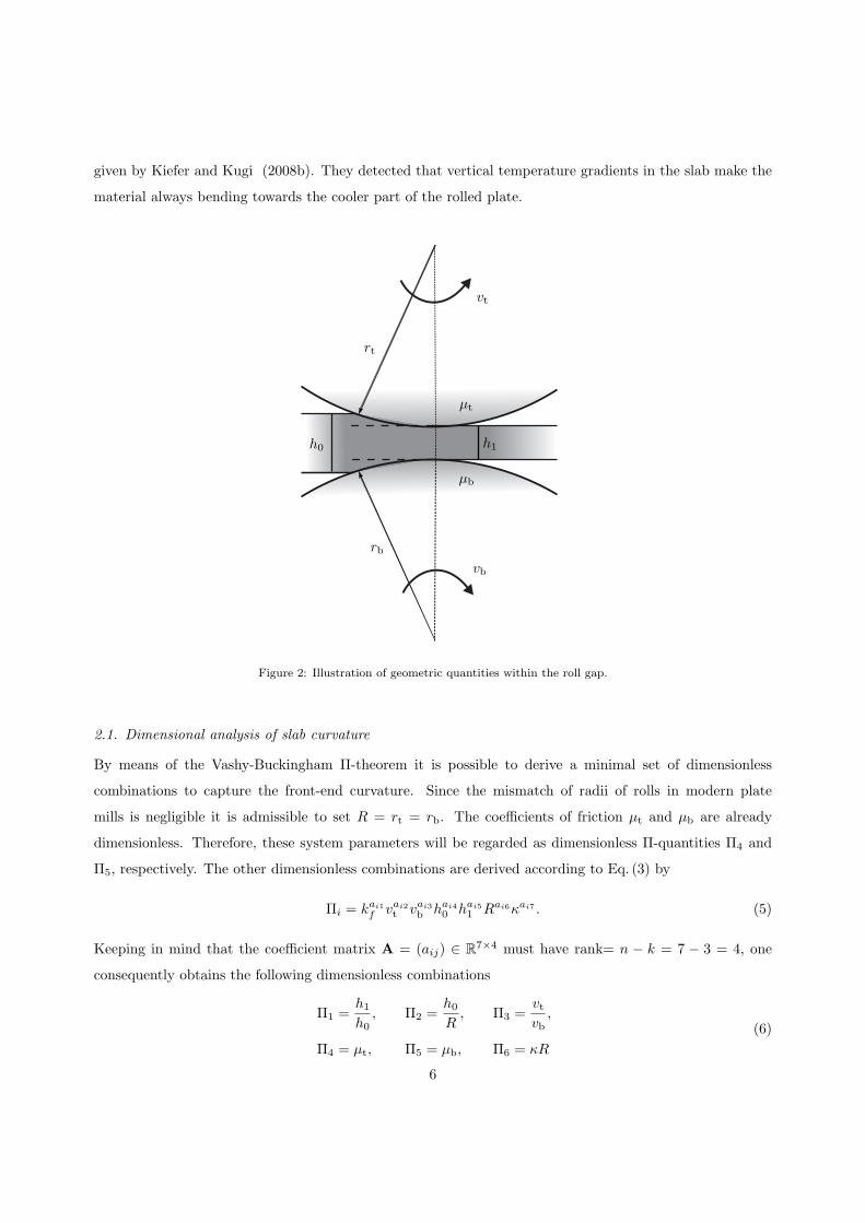
given by Kiefer and Kugi (2008b). They detected that vertical temperature gradients in the slab make the
material always bending towards the cooler part of the rolled plate.
µt
µb
h0 h1
rt
rb
vt
vb
Figure 2: Illustration of geometric quantities within the roll gap.
2.1. Dimensional analysis of slab curvature
By means of the Vashy-Buckingham Π-theorem it is possible to derive a minimal set of dimensionless
combinations to capture the front-end curvature. Since the mismatch of radii of rolls in modern plate
mills is negligible it is admissible to set R = rt = rb. The coefficients of friction µt and µb are already
dimensionless. Therefore, these system parameters will be regarded as dimensionless Π-quantities Π4 and
Π5, respectively. The other dimensionless combinations are derived according to Eq. (3) by
Πi = kai1
f vai2
t vai3
b hai4
0 hai5
1 Rai6κai7 . (5)
Keeping in mind that the coefficient matrix A = (aij) ∈ R7×4 must have rank= n − k = 7 − 3 = 4, one
consequently obtains the following dimensionless combinations
Π1 =h1
h0, Π2 =
h0
R, Π3 =
vtvb
,
Π4 = µt, Π5 = µb, Π6 = κR
(6)
6

with the corresponding coefficient matrix
A =
0 0 0 −1 1 0 0
0 0 0 1 0 −1 0
0 1 −1 0 0 0 0
0 0 0 0 0 1 1
. (7)
For the construction of dimensionless Π-numbers it is appropriate to combine similar physical quantities
such as length type terms, velocity type terms, etc. However, Π1 and Π2 contain all relevant geometric
quantities of the roll gap. In many technical applications the relative pass reduction
εh = 1−h1
h0= 1−Π1 (8)
is often used to measure the geometry of the roll gap. For a constant R the quantity Π2 is proportional to the
height of the rolled stock. The Π-number Π3 indicates the speed mismatch. The dimensionless combination
Π6 ∈ [−1, 1] measures the curvature of the plate where it is −1 or 1 if and only if the rolled slab has the
same curvature as the bottom or the upper roll, respectively.
2.2. Dimensionless combinations for technological quantities
Likewise the calculations in Section 2.1 it is possible to derive dimensionless combinations for technological
quantities such as the rolling torque of the upper/bottom roll Mt/Mb and the rolling force F . These phys-
ical quantities can actually be measured during the forming process. For this reason, they are denoted as
technological quantities.
Please note that here the dimensionless combinations Π1,Π2, . . . ,Π6 are retained from the previous consid-
erations. Analogously to the previous section the additional dimensionless combinations involving force and
torque type terms are given by
Π7 =Mt
kfR3, Π8 =
Mb
kfR3, Π9 =
F
kfR2. (9)
The radius of the upper and bottom roll acts here as a geometrical reference value. In this manner the
calculated Π-values are always related to the geometry of the rolls which take the forces and torques from
the forming process.
The established dimensionless combinations from this section will serve as basis for the parametric studies
in the sections below.
3. Finite element simulation
This section deals with a systematic finite element approach to the phenomenon of front-end bending by
means of the dimensionless combinations from the previous part of the manuscript. Although numerous7
investigations on front-end bending in plate rolling applications have been published in the past, according
to Philipp et al. (2007) operators are still struggling with the problem. Therefore, detailed parametric
studies will be provided here. These studies may be employed as reference for online implementation of
control mechanisms during the forming process.
3.1. Finite element model
In the scope of this work the numerical simulations are performed by means of the commercial finite element
software MSC.Marc/Mentat. Within the framework of this finite element model the work rolls are
regarded as ideally rigid bodies rotating with the constant circumferential velocities vt and vb, respectively.
The distance between the rolls is h1. The roll table is modeled as a straight line which uniformly directs the
slab into the roll gap and inhibits the movement of the slab in vertical direction. The friction between roll
table and slab is neglected. The slab has the height h0 and is modeled as a deformable body. Consequently,
isoparametric quadrilateral elements with linear shape functions for the spatial discretization of the slab
are employed. The velocity vs of the slab is initially set to the mean velocity of vt and vb. Later on,
the velocity of the slab is controlled by the angular velocities of the rolls so that the initial velocity vs
which is necessary to initialize the contact of the slab with the rolls does not affect the result of the
simulation. The numerical algorithm for the contact between the slab and the upper/bottom work roll
involves the Coulomb law of friction by means of friction coefficients µt/µb. For the sake of simplicity
three-dimensional deformation phenomena such as spreading of the processed material within the roll gap
are neglected. Therefore, a plane strain state in the two-dimensional Euclidean space characterized by
spatial coordinates x := x1e1 + x2e2 = (x1, x2) may be assumed. Here, the basis vector e1 points into
the horizontal rolling direction and e2 denotes the vertical direction referring to the height of the rolled
sheet. Let v = ∂x/∂t ∈ R2 be the spatial velocity field and σ ∈ R
3×3 denotes the Cauchy stress tensor.
In classical metal forming calculations external body forces like gravitational forces are neglected and the
processed material is assumed to be incompressible. In terms of continuum mechanics these requirements
are expressed for the quasi-static regime by means of the mass balance and the balance of linear momentum
as follows
div (v) = 0, (10)
div (σ) = 0. (11)
As constitutive equation for the considered plastic deformation the classical von Mises flow rule
f =
∥
∥
∥
∥
1
2
(
σ −1
3tr (σ)
)∥
∥
∥
∥
− kf (12)
is used. After the yield stress kf is reached the deformation of material is assumed to behave ideally rigid-
plastic. Strain hardening as well as viscoplasticity are not considered in this model. Therefore, the system of8
partial differential equations (10)-(12) subjected to given boundary conditions has to be solved. Please note
that high computational costs as mentioned in Kiefer and Kugi (2008b) could be reduced with a coarser
mesh in the areas which do not undergo a deformation in the roll gap. A very similar finite element model is
used by Kiefer and Kugi (2008b) for the validation of their upper bound approach and by Richelsen (1997)
to analyze the stress/strain distribution within the roll gap.
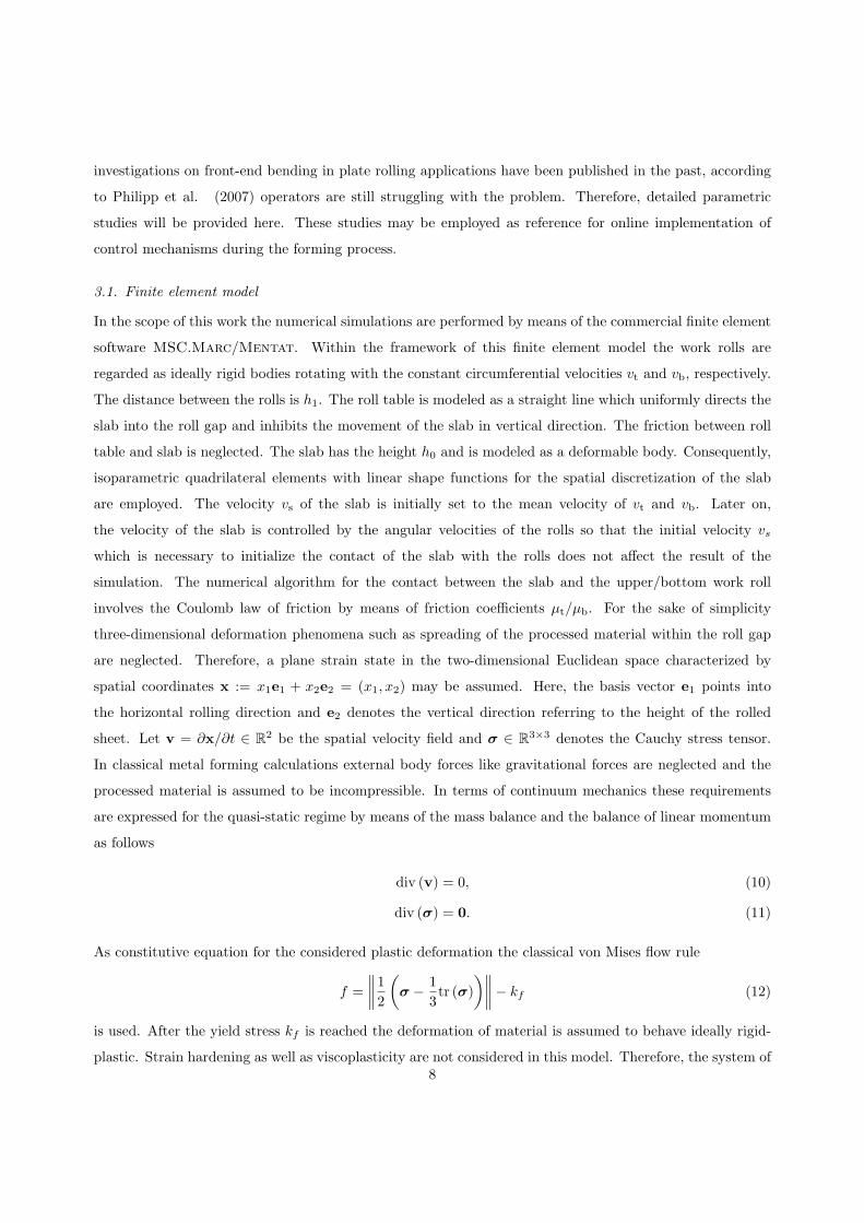
The result of one simulation is shown in Fig. 3. One can see the bending of the plate towards the upper roll
and the asymmetric distribution of the slab’s velocities over the roll gap.
Figure 3: Illustration of finite element simulation results for the asymmetric rolling process with local velocities [mm/s].
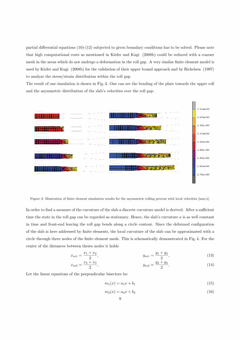
In order to find a measure of the curvature of the slab a discrete curvature model is derived. After a sufficient
time the state in the roll gap can be regarded as stationary. Hence, the slab’s curvature κ is as well constant
in time and front-end leaving the roll gap bends along a circle contour. Since the deformed configuration
of the slab is here addressed by finite elements, the local curvature of the slab can be approximated with a
circle through three nodes of the finite element mesh. This is schematically demonstrated in Fig. 4. For the
center of the distances between theses nodes it holds
xm1 =x1 + x2
2, ym1 =
y1 + y22
, (13)
xm2 =x2 + x3
2, ym2 =
y2 + y32
. (14)
Let the linear equations of the perpendicular bisectors be:
m1(x) = a1x+ b1 (15)
m2(x) = a2x+ b2 (16)
9
(x1, y1)
(xm1, ym1) (x2, y2)
(xm2, ym2)
(x3, y3)
(xmk, ymk)
x
y
Figure 4: Schematic derivation of a discrete measure for curvature.
For the slopes and the axis intercepts one obtain:
a1 =x1 − x2
y2 − y1b1 = ym1 − a1xm1 (17)
a2 =x2 − x3
y3 − y2b2 = ym2 − a2xm2 (18)
The center of the circle (xmk, ymk) is the intersection point of the perpendicular bisectors.
a1xmk + b1 = a2xmk + b2 (19)
⇔ xmk =b2 − b1a1 − a2
(20)
For ymk it ensues
ymk = m1(xmk). (21)
The radius of the circle directly follows from the distance of the center point to an arbitrary construction
point. Since the curvature of the slab is the reciprocal of the circle’s radius, κ can be calculated according
to
κ =1
√
(ymk − y2)2+ (xmk − x2)
2(22)
3.2. Parametric studies
In the sequel, detailed parametric studies will be performed in order to get a deeper insight into front-
end bending in plate rolling applications. Starting from the above-mentioned finite element model the
following studies are embedded into a discrete parameter space spanned by the dimensionless combinations
Π1,Π2,Π3,Π4 and Π5. Whilst taking into account the technically relevant range for geometric quanti-
ties, speed mismatch and coefficients of friction between the upper and lower work roll and the material,
10

respectively, leads to the following parametric grid
Π1 = [0.70, 0.75, 0.80, 0.85, 0.90, 0.95]
Π2 = [0.02, 0.04, 0.06, 0.08, 0.10]
Π3 = [1.00, 1.01, 1.025, 1.05]
Π4 = [0.30, 0.40, 0.50]
Π5 = [0.30, 0.40, 0.50]
(23)
Please note that for equal circumferential velocities vt = vb (Π3 = 1) and equal coefficients of frictions
µt = µb (Π4 = Π5) the forming process is fully symmetric and there is actually no front-end bending.
The mathematical quantification of the ski effect is done in terms of the dimensionless combination Π6 which
is proportional to the curvature κ. In the presented framework, a negative value of Π6 indicates that the
slab bends towards the bottom work roll.
3.2.1. Impact of friction conditions
Here the effect of the level of friction coefficients on the slab curvature at a fixed speed mismatch of 5%
is studied. The simulation results are presented in two dimensional countour plots on Π1 × Π2 illustrating
respective isolines. In the first setting symmetric friction conditions subjected to the above-mentioned speed
mismatch are considered. The results are shown in Figs. 5 – 7.
−0.8
−0.8
−0.6
−0.6
−0.4
−0.4
−0.4−0.2
−0.2
−0.2
−0.20
0
0
00.2
0.2
0.2
0.2
0.4
0.4
0.4
0.4
0.40.6
0.6
0.6
0.6
0.6
0.6
0.8
0.8
0.8
0.7 0.75 0.8 0.85 0.9 0.950.02
0.03
0.04
0.05
0.06
0.07
0.08
0.09
0.1
Π5 = 0.3
Π4 = 0.3
Π3 = 1.05
Π1
Π2
Figure 5: Illustration of Π6 for Π4 = Π5 = 0.3 for a speed mismatch of 5%.
11

−0.8
−0.8
−0.6
−0.6
−0.6
−0.4
−0.4
−0.4
−0.4−0.2
−0.2
−0.2
−0.2
0
0
0
0
0.2
0.2
0.2
0.2
0.20.4
0.4
0.4
0.4
0.4
0.6
0.6
0.6
0.6
0.6
0.80.8
0.7 0.75 0.8 0.85 0.9 0.950.02
0.03
0.04
0.05
0.06
0.07
0.08
0.09
0.1
Π5 = 0.4
Π4 = 0.4
Π3 = 1.05
Π1
Π2
Figure 6: Illustration of Π6 for Π4 = Π5 = 0.4 for a speed mismatch of 5%.
−0.8
−0.8
−0.8
−0.6
−0.6
−0.6
−0.4
−0.4
−0.4
−0.4−0.2
−0.2
−0.2
−0.20
0
0
0
0.2
0.2
0.2
0.2
0.2
0.4
0.4
0.4
0.4
0.40.6
0.6 0.6
0.60.8 0.8
0.7 0.75 0.8 0.85 0.9 0.950.02
0.03
0.04
0.05
0.06
0.07
0.08
0.09
0.1
Π5 = 0.4
Π4 = 0.4
Π3 = 1.05
Π5 = 0.5
Π4 = 0.5
Π3 = 1.05
Π1
Π2
Figure 7: Illustration of Π6 for Π4 = Π5 = 0.5 for a speed mismatch of 5%.
These results nicely reproduce the interesting fact that the curvature of the outgoing plate does not only
depend on the asymmetric rolling conditions but also on the roll gap geometry, which has also been observed
by Philipp et al. (2007) and Kiefer and Kugi (2008a). So far, it generally had been assumed that for plate
rolling applications subjected to a speed mismatch of the work rolls the slab bends away from the faster roll
for small thickness reductions and towards the faster roll for larger thickness reductions. This is actually
the case for (Π1,Π2) ∈ [0.80, 0.95] × [0.04, 0.10]. Surprisingly, the presented studies detect a further purely
geometrical parameter setting with (Π1,Π2) ∈ [0.7, 0.75]× [0.02, 0.03] where the curvature is negative again.
This result indicates that front-end bending is an extremely complex and highly nonlinear phenomenon,
which is rather difficult to handle at the first glance.
The differences between Figs. 5 – 7 are very small, because the isoline where there is a change of sign of
the curvature marginally varies. Therefore, one may state that the level of friction coefficients has a minor
influence on the ski effect.
12
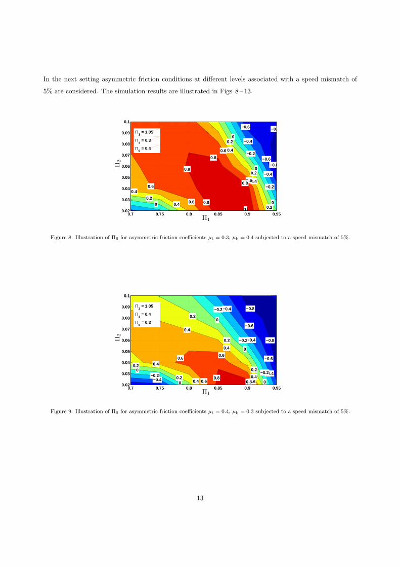
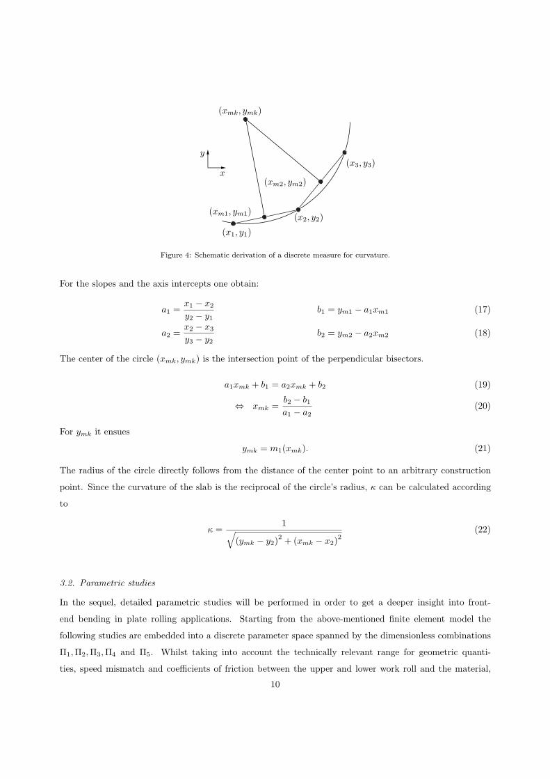
In the next setting asymmetric friction conditions at different levels associated with a speed mismatch of
5% are considered. The simulation results are illustrated in Figs. 8 – 13.
−0.8
−0.8
−0.6
−0.6
−0.4
−0.4
−0.2
−0.2
0
0
0
00.2
0.2
0.2
0.20.4
0.4
0.4
0.4
0.6
0.6
0.6
0.6
0.8
0.8
0.8
0.8
10.7 0.75 0.8 0.85 0.9 0.95
0.02
0.03
0.04
0.05
0.06
0.07
0.08
0.09
0.1
Π5 = 0.4
Π4 = 0.3
Π3 = 1.05
Π1
Π2
Figure 8: Illustration of Π6 for asymmetric friction coefficients µt = 0.3, µb = 0.4 subjected to a speed mismatch of 5%.
−0.8
−0.8
−0.6
−0.6
−0.4
−0.4
−0.4
−0.4−0.2
−0.2
−0.2
−0.2
0
0
0
0
00.2
0.2
0.2
0.2
0.2
0.4
0.4
0.4
0.4
0.4
0.40.6
0.60.6
0.60.8
0.80.7 0.75 0.8 0.85 0.9 0.95
0.02
0.03
0.04
0.05
0.06
0.07
0.08
0.09
0.1
Π5 = 0.3
Π4 = 0.4
Π3 = 1.05
Π5 = 0.5
Π4 = 0.5
Π3 = 1.05
Π5 = 0.3
Π4 = 0.4
Π3 = 1.05
Π1
Π2
Figure 9: Illustration of Π6 for asymmetric friction coefficients µt = 0.4, µb = 0.3 subjected to a speed mismatch of 5%.
13
−0.8
−0.8
−0.6
−0.6
−0.6
−0.4
−0.4
−0.4−0.2
−0.2
−0.2
−0.20
0
0
0
0.2
0.2
0.2
0.20.4
0.4
0.4
0.4
0.40.6
0.6
0.6 0.6
0.6
0.60.8
0.8
0.8
0.7 0.75 0.8 0.85 0.9 0.950.02
0.03
0.04
0.05
0.06
0.07
0.08
0.09
0.1
Π5 = 0.5
Π4 = 0.4
Π3 = 1.05
Π1
Π2
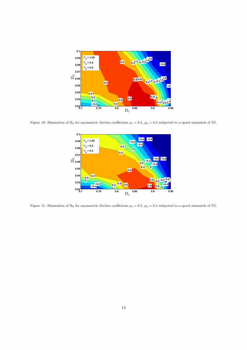
Figure 10: Illustration of Π6 for asymmetric friction coefficients µt = 0.4, µb = 0.5 subjected to a speed mismatch of 5%.
−0.8
−0.8
−0.8
−0.6
−0.6
−0.6
−0.4
−0.4
−0.4
−0.4−0.2
−0.2
−0.2
−0.2
0
0
0
0
00.2
0.2
0.2
0.2
0.20.4
0.4
0.4
0.4
0.4
0.40.6
0.6
0.6
0.8
0.7 0.75 0.8 0.85 0.9 0.950.02
0.03
0.04
0.05
0.06
0.07
0.08
0.09
0.1
Π5 = 0.5
Π4 = 0.4
Π3 = 1.05
Π5 = 0.4
Π4 = 0.5
Π3 = 1.05
Π1
Π2
Figure 11: Illustration of Π6 for asymmetric friction coefficients µt = 0.5, µb = 0.4 subjected to a speed mismatch of 5%.
14
−0.8
−0.6
−0.6
−0.4
−0.4
−0.2
−0.2
0
0
0
0.2
0.2
0.2
0.20.4
0.4
0.4
0.4
0.6
0.6
0.6
0.6
0.6
0.8
0.8
0.8
0.8
0.8
0.8
10.7 0.75 0.8 0.85 0.9 0.95
0.02
0.03
0.04
0.05
0.06
0.07
0.08
0.09
0.1
Π5 = 0.5
Π4 = 0.3
Π3 = 1.05
Π1
Π2
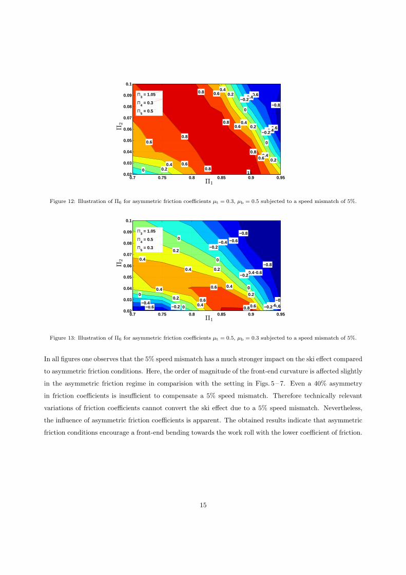
Figure 12: Illustration of Π6 for asymmetric friction coefficients µt = 0.3, µb = 0.5 subjected to a speed mismatch of 5%.
−0.8
−0.8
−0.8
−0.6
−0.6
−0.6
−0.6−0.4
−0.4
−0.4
−0.4−0.2
−0.2
−0.2
−0.20
0
0
0
0
0.2
0.2
0.2
0.2
0.4
0.4
0.4
0.4
0.4
0.6
0.6
0.60.80.7 0.75 0.8 0.85 0.9 0.95
0.02
0.03
0.04
0.05
0.06
0.07
0.08
0.09
0.1
Π5 = 0.3
Π4 = 0.5
Π3 = 1.05
Π1
Π2
Figure 13: Illustration of Π6 for asymmetric friction coefficients µt = 0.5, µb = 0.3 subjected to a speed mismatch of 5%.
In all figures one observes that the 5% speed mismatch has a much stronger impact on the ski effect compared
to asymmetric friction conditions. Here, the order of magnitude of the front-end curvature is affected slightly
in the asymmetric friction regime in comparision with the setting in Figs. 5 – 7. Even a 40% asymmetry
in friction coefficients is insufficient to compensate a 5% speed mismatch. Therefore technically relevant
variations of friction coefficients cannot convert the ski effect due to a 5% speed mismatch. Nevertheless,
the influence of asymmetric friction coefficients is apparent. The obtained results indicate that asymmetric
friction conditions encourage a front-end bending towards the work roll with the lower coefficient of friction.
15
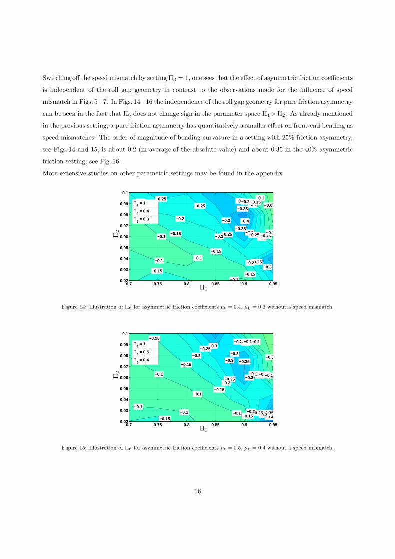
Switching off the speed mismatch by setting Π3 = 1, one sees that the effect of asymmetric friction coefficients
is independent of the roll gap geometry in contrast to the observations made for the influence of speed
mismatch in Figs. 5 – 7. In Figs. 14 – 16 the independence of the roll gap geometry for pure friction asymmetry
can be seen in the fact that Π6 does not change sign in the parameter space Π1×Π2. As already mentioned
in the previous setting, a pure friction asymmetry has quantitatively a smaller effect on front-end bending as
speed mismatches. The order of magnitude of bending curvature in a setting with 25% friction asymmetry,
see Figs. 14 and 15, is about 0.2 (in average of the absolute value) and about 0.35 in the 40% asymmetric
friction setting, see Fig. 16.
More extensive studies on other parametric settings may be found in the appendix.
−0.3
−0.3
−0.3
−0.3
−0.25
−0.25
−0.25 −0.25
−0.25
−0.25
−0.2
−0.2
−0.2
−0.2
−0.15
−0.15
−0.15
−0.15−0.15
−0.1
−0.1−0.1
−0.2
−0.2
−0.15
−0.15
−0.1
−0.1
−0.35
−0.35−0.05
−0.4
−0.10.7 0.75 0.8 0.85 0.9 0.95
0.02
0.03
0.04
0.05
0.06
0.07
0.08
0.09
0.1
Π5 = 0.3
Π4 = 0.4
Π3 = 1
Π1
Π2
Figure 14: Illustration of Π6 for asymmetric friction coefficients µt = 0.4, µb = 0.3 without a speed mismatch.
−0.4−0.35
−0.3
−0.3
−0.25
−0.25−0.25
−0.25
−0.25
−0.2
−0.2
−0.2
−0.15
−0.15
−0.15
−0.15
−0.15−0.1
−0.1
−0.1
−0.1
−0.1
−0.2
−0.2
−0.15
−0.15
−0.3
−0.3
−0.3
−0.1
−0.1
−0.05−0.35
0.7 0.75 0.8 0.85 0.9 0.950.02
0.03
0.04
0.05
0.06
0.07
0.08
0.09
0.1
Π5 = 0.4
Π4 = 0.5
Π3 = 1
Π1
Π2
Figure 15: Illustration of Π6 for asymmetric friction coefficients µt = 0.5, µb = 0.4 without a speed mismatch.
16
−0.5
−0.5−0.5
−0.5
−0.5
−0.4
−0.4
−0.4
−0.4
−0.3
−0.3
−0.3
−0.3−0.3
−0.2
−0.2−0.2
−0.4
−0.4
−0.3
−0.3
−0.2
−0.2
−0.6
−0.6
−0.2
−0.1
0.7 0.75 0.8 0.85 0.9 0.950.02
0.03
0.04
0.05
0.06
0.07
0.08
0.09
0.1
Π5 = 0.3
Π4 = 0.5
Π3 = 1
Π1
Π2
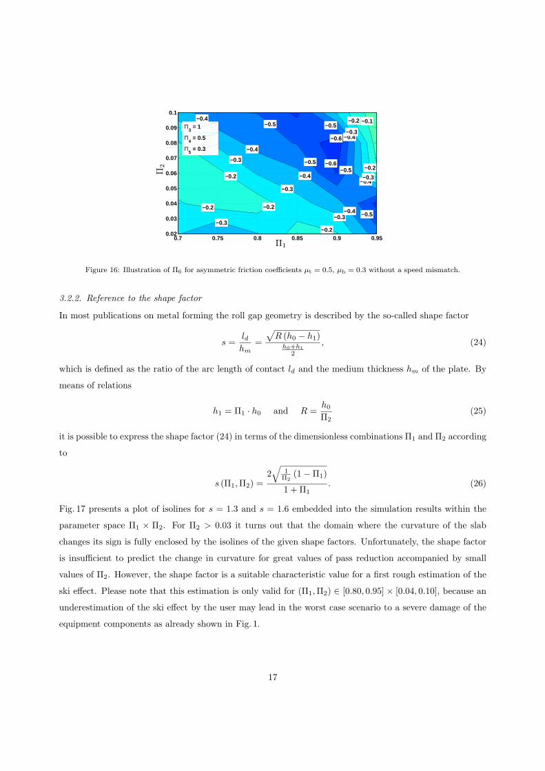
Figure 16: Illustration of Π6 for asymmetric friction coefficients µt = 0.5, µb = 0.3 without a speed mismatch.
3.2.2. Reference to the shape factor
In most publications on metal forming the roll gap geometry is described by the so-called shape factor
s =ldhm
=
√
R (h0 − h1)h0+h1
2
, (24)
which is defined as the ratio of the arc length of contact ld and the medium thickness hm of the plate. By
means of relations
h1 = Π1 · h0 and R =h0
Π2(25)
it is possible to express the shape factor (24) in terms of the dimensionless combinations Π1 and Π2 according
to
s (Π1,Π2) =2√
1Π2
(1−Π1)
1 + Π1. (26)
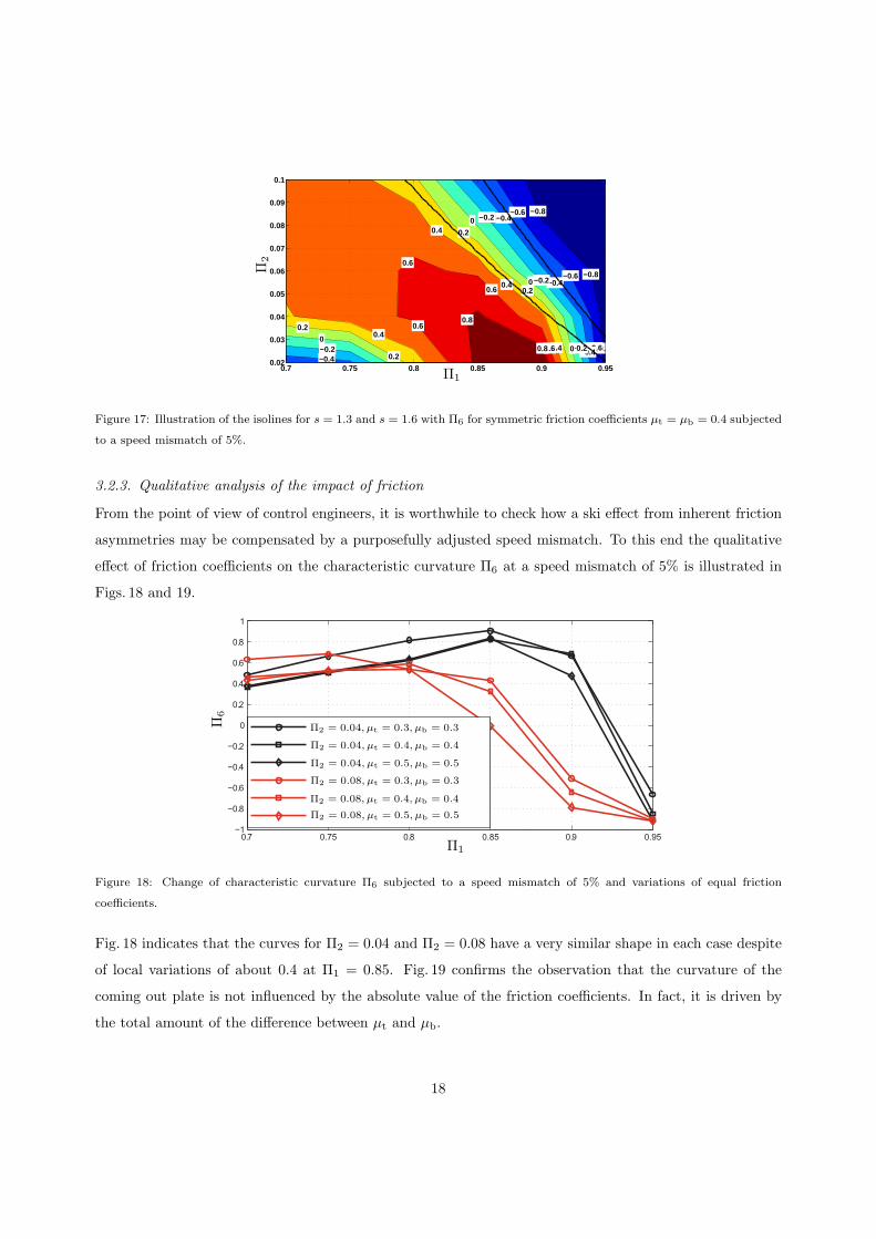
Fig. 17 presents a plot of isolines for s = 1.3 and s = 1.6 embedded into the simulation results within the
parameter space Π1 × Π2. For Π2 > 0.03 it turns out that the domain where the curvature of the slab
changes its sign is fully enclosed by the isolines of the given shape factors. Unfortunately, the shape factor
is insufficient to predict the change in curvature for great values of pass reduction accompanied by small
values of Π2. However, the shape factor is a suitable characteristic value for a first rough estimation of the
ski effect. Please note that this estimation is only valid for (Π1,Π2) ∈ [0.80, 0.95] × [0.04, 0.10], because an
underestimation of the ski effect by the user may lead in the worst case scenario to a severe damage of the
equipment components as already shown in Fig. 1.
17
−0.8
−0.8
−0.8
−0.6
−0.6
−0.6−0.4
−0.4
−0.4
−0.4−0.2
−0.2
−0.2
−0.20
0
0
00.2
0.2
0.2
0.2
0.4
0.4
0.4
0.4
0.6
0.6
0.6
0.6
0.8
0.8
0.7 0.75 0.8 0.85 0.9 0.950.02
0.03
0.04
0.05
0.06
0.07
0.08
0.09
0.1
Π1
Π2
Figure 17: Illustration of the isolines for s = 1.3 and s = 1.6 with Π6 for symmetric friction coefficients µt = µb = 0.4 subjected
to a speed mismatch of 5%.
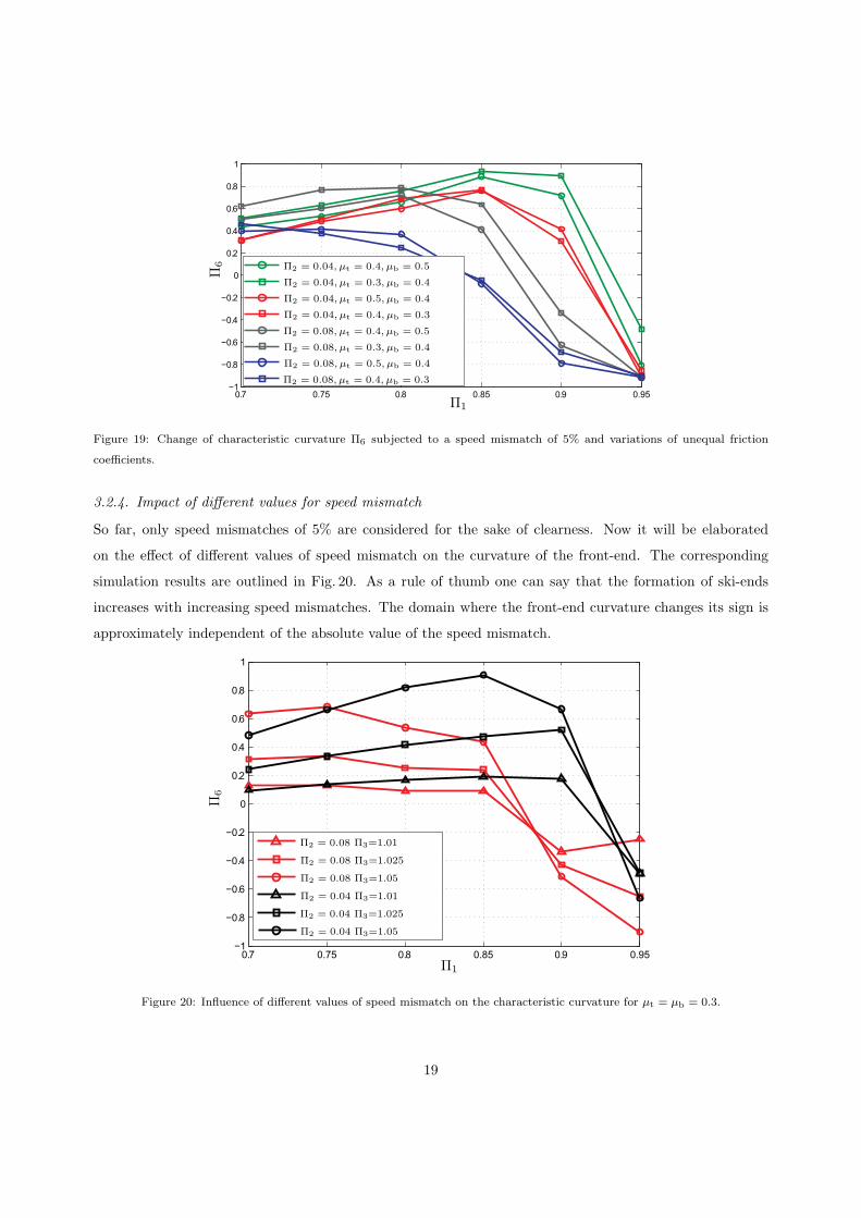
3.2.3. Qualitative analysis of the impact of friction
From the point of view of control engineers, it is worthwhile to check how a ski effect from inherent friction
asymmetries may be compensated by a purposefully adjusted speed mismatch. To this end the qualitative
effect of friction coefficients on the characteristic curvature Π6 at a speed mismatch of 5% is illustrated in
Figs. 18 and 19.
0.7 0.75 0.8 0.85 0.9 0.95−1
−0.8
−0.6
−0.4
−0.2
0
0.2
0.4
0.6
0.8
Π1
Π6
Π2 = 0.04,µt = 0.3,µb = 0.3
Π2 = 0.04,µt = 0.4,µb = 0.4
Π2 = 0.04,µt = 0.5,µb = 0.5
Π2 = 0.08,µt = 0.3,µb = 0.3
Π2 = 0.08,µt = 0.4,µb = 0.4
Π2 = 0.08,µt = 0.5,µb = 0.5
Figure 18: Change of characteristic curvature Π6 subjected to a speed mismatch of 5% and variations of equal friction
coefficients.
Fig. 18 indicates that the curves for Π2 = 0.04 and Π2 = 0.08 have a very similar shape in each case despite
of local variations of about 0.4 at Π1 = 0.85. Fig. 19 confirms the observation that the curvature of the
coming out plate is not influenced by the absolute value of the friction coefficients. In fact, it is driven by
the total amount of the difference between µt and µb.
18
0.7 0.75 0.8 0.85 0.9 0.95−1
−0.8
−0.6
−0.4
−0.2
0
0.2
0.4
0.6
0.8
Π1
Π6 Π2 = 0.04,µt = 0.4,µb = 0.5
Π2 = 0.04,µt = 0.3,µb = 0.4
Π2 = 0.04,µt = 0.5,µb = 0.4
Π2 = 0.04,µt = 0.4,µb = 0.3
Π2 = 0.08,µt = 0.4,µb = 0.5
Π2 = 0.08,µt = 0.3,µb = 0.4
Π2 = 0.08,µt = 0.5,µb = 0.4
Π2 = 0.08,µt = 0.4,µb = 0.3
Figure 19: Change of characteristic curvature Π6 subjected to a speed mismatch of 5% and variations of unequal friction
coefficients.
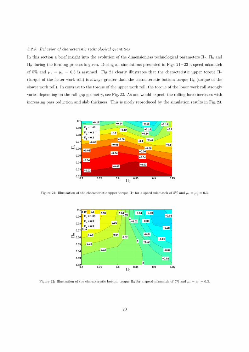
3.2.4. Impact of different values for speed mismatch
So far, only speed mismatches of 5% are considered for the sake of clearness. Now it will be elaborated
on the effect of different values of speed mismatch on the curvature of the front-end. The corresponding
simulation results are outlined in Fig. 20. As a rule of thumb one can say that the formation of ski-ends
increases with increasing speed mismatches. The domain where the front-end curvature changes its sign is
approximately independent of the absolute value of the speed mismatch.
0.7 0.75 0.8 0.85 0.9 0.95−1
−0.8
−0.6
−0.4
−0.2
0
0.2
0.4
0.6
0.8
Π1
Π6
Π2 = 0.08 Π3=1.01
Π2 = 0.08 Π3=1.025
Π2 = 0.08 Π3=1.05
Π2 = 0.04 Π3=1.01
Π2 = 0.04 Π3=1.025
Π2 = 0.04 Π3=1.05
Figure 20: Influence of different values of speed mismatch on the characteristic curvature for µt = µb = 0.3.
19
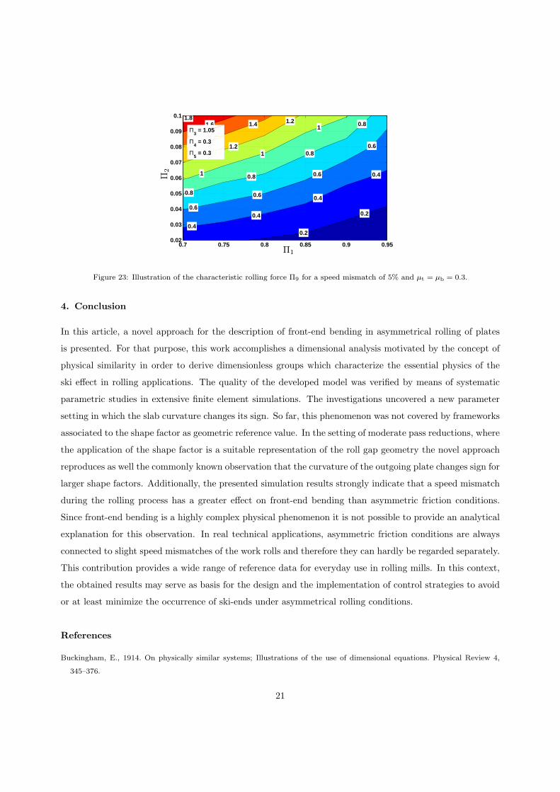
3.2.5. Behavior of characteristic technological quantities
In this section a brief insight into the evolution of the dimensionless technological parameters Π7, Π8 and
Π9 during the forming process is given. During all simulations presented in Figs. 21 – 23 a speed mismatch
of 5% and µt = µb = 0.3 is assumed. Fig. 21 clearly illustrates that the characteristic upper torque Π7
(torque of the faster work roll) is always greater than the characteristic bottom torque Π8 (torque of the
slower work roll). In contrast to the torque of the upper work roll, the torque of the lower work roll strongly
varies depending on the roll gap geometry, see Fig. 22. As one would expect, the rolling force increases with
increasing pass reduction and slab thickness. This is nicely reproduced by the simulation results in Fig. 23.
−0.18−0.16
−0.16−0.14
−0.14
−0.14
−0.14
−0.12 −0.12
−0.12
−0.12
−0.1
−0.1
−0.1−0.1
−0.08−0.08
−0.08−0.06
−0.06
−0.06
−0.04
−0.04
−0.04
−0.02
−0.02−0.02
0.7 0.75 0.8 0.85 0.9 0.950.02
0.03
0.04
0.05
0.06
0.07
0.08
0.09
0.1
Π5 = 0.3
Π4 = 0.3
Π3 = 1.05
Π1
Π2
Figure 21: Illustration of the characteristic upper torque Π7 for a speed mismatch of 5% and µt = µb = 0.3.
−0.08
−0.08
−0.06
−0.06
−0.04
−0.04
−0.04
−0.02
−0.02
−0.02
0
0
0
0.02
0.02
0.02
0.04
0.04
0.04
0.06
0.06
0.08
0.08
0.1−0.08
0.12
0.7 0.75 0.8 0.85 0.9 0.950.02
0.03
0.04
0.05
0.06
0.07
0.08
0.09
0.1
Π5 = 0.3
Π4 = 0.3
Π3 = 1.05
Π1
Π2
Figure 22: Illustration of the characteristic bottom torque Π8 for a speed mismatch of 5% and µt = µb = 0.3.
20
0.2
0.2
0.4
0.4
0.4
0.4
0.6
0.6
0.6
0.6
0.8
0.8
0.8
0.8
1
1
1
1.2
1.2
1.4
1.4
1.61.8
0.7 0.75 0.8 0.85 0.9 0.950.02
0.03
0.04
0.05
0.06
0.07
0.08
0.09
0.1
Π5 = 0.3
Π4 = 0.3
Π3 = 1.05
Π1
Π2
Figure 23: Illustration of the characteristic rolling force Π9 for a speed mismatch of 5% and µt = µb = 0.3.
4. Conclusion
In this article, a novel approach for the description of front-end bending in asymmetrical rolling of plates
is presented. For that purpose, this work accomplishes a dimensional analysis motivated by the concept of
physical similarity in order to derive dimensionless groups which characterize the essential physics of the
ski effect in rolling applications. The quality of the developed model was verified by means of systematic
parametric studies in extensive finite element simulations. The investigations uncovered a new parameter
setting in which the slab curvature changes its sign. So far, this phenomenon was not covered by frameworks
associated to the shape factor as geometric reference value. In the setting of moderate pass reductions, where
the application of the shape factor is a suitable representation of the roll gap geometry the novel approach
reproduces as well the commonly known observation that the curvature of the outgoing plate changes sign for
larger shape factors. Additionally, the presented simulation results strongly indicate that a speed mismatch
during the rolling process has a greater effect on front-end bending than asymmetric friction conditions.
Since front-end bending is a highly complex physical phenomenon it is not possible to provide an analytical
explanation for this observation. In real technical applications, asymmetric friction conditions are always
connected to slight speed mismatches of the work rolls and therefore they can hardly be regarded separately.
This contribution provides a wide range of reference data for everyday use in rolling mills. In this context,
the obtained results may serve as basis for the design and the implementation of control strategies to avoid
or at least minimize the occurrence of ski-ends under asymmetrical rolling conditions.
References
Buckingham, E., 1914. On physically similar systems; Illustrations of the use of dimensional equations. Physical Review 4,
345–376.
21

Farhat-Nia, F., Salimi, M., Movahhedy, M.R., 2006. Elasto-plastic finite element simulation of asymmetrical plate rolling using
an ALE approach. Journal of Materials Processing Technology 177, 525–529.
Hwang, Y.-M., Tzou, G.-Y., 1993. An analytical approach to asymmetrical cold strip rolling using the slab method. Journal of
Engineering and Performance 2, 597–606.
Harrer, O., Philipp, M., Pokorny, I., 2003. Numerical simulation of asymmetric effects in plate rolling. Acta Metallurgica
Slovaca 9, 306–313.
Hwang, Y.-M., Tzou, G.-Y., 1995. An analytical approach to asymmetrical hot-sheet rolling considering the effects of the shear
stress and internal moment at the roll gap. Journal of Materials Processing Technology 52, 399–424.
Jeswiet, J., Greene, P.G., 1998. Experimental measurement of curl in rolling. Journal of Materials Processing Technology 84,
202–209.
Kazeminezhad, M., Karimi Taheri, A., 2005. An experimental investigation on the deformation behavior during wire flat rolling
process. Journal of Materials Processing Technology 160, 313–320.
Kiefer, T., Kugi, A., 2008a. An analytical approach for modelling asymmetrical hot rolling of heavy plates. Mathematical and
Computer Modelling of Dynamical Systems 14(3), 249–267.
Kiefer, T., Kugi, A., 2008b. Model-based control of front-end bending in hot rolling processes. Vortrag: 17th World Congress,
The International Federation of Automatic Control, ; 06.07.2008 - 11.07.2008; In: ”Proceedings of the 17th World Congress,
The International Federation of Automatic Control, Seoul, Korea, July 6–11, ISSN: 1474–6670; pp. 1645–1650.
Pan, D., Sansome, D.H., 1982. An experimental study of the effect of roll-speed mismatch on the rolling load during the cold
rolling of thin strip. Journal of Mechanical Working Technology 6, 361–377.
Pawelski, O., 1992. Ways and limits of the theory of similarity in application to problems of physics and metal forming. Journal
of Materials Processing Technology 34(1–4), 19–30.
Pawelski, O., 1993. Ahnlichkeitstheorie in der Umformtechnik. In: Dahl, W., Kopp, R., Pawelski, O. (Eds.), Umformtechnik,
Plastomechanik und Werkstoffkunde. Berlin, Springer, ISBN 3-50-56682-1, pp. 158–176
Pawelski, H., 2000. Comparison of methods for calculating the influence of asymmetry in strip and plate rolling. Steel research
71, 490–496.
Philipp, M., Schwenzfeier, W., Fischer, F.D., Wodlinger, R., Fischer, C., 2007. Front end bending in plate rolling influenced
by circumferential speed mismatch and geometry. Journal of Materials Processing Technology 184(1–3), 224–232.
Richelsen, A.B., 1997. Elastic-plastic analysis of the stress and strain distributions in asymmetric rolling, International Journal
of Mechanical Sciences 39(11), 1199–1211.
Salimia, M., Sassani, F., 2002. Modified slab analysis of asymmetrical plate rolling. International Journal of Mechanical Sciences
44, 1999–2023.
Taylor, B.N., Thompson, A., Editors, 2008. The International System of Units (SI). National Institute of Standards and
Technology Special Publication 330.
Vaschy, A., 1892. Sur les lois de similitude en physique. Annales Telegraphiques (troisieme serie) 19, 25–28.
Appendix A. Diagrams of curvature coefficient Π6 at different settings
This appendix will provide the reader with additional results on characteristic curvature Π6 for various
parameter settings.
Appendix A.1. Results for 2.5% speed mismatch
The first section focuses on front-end bending for a 2.5% speed mismatch subjected to different friction condi-
tions. Throughout the simulation results it can be observed that for moderate values of the speed mismatch22
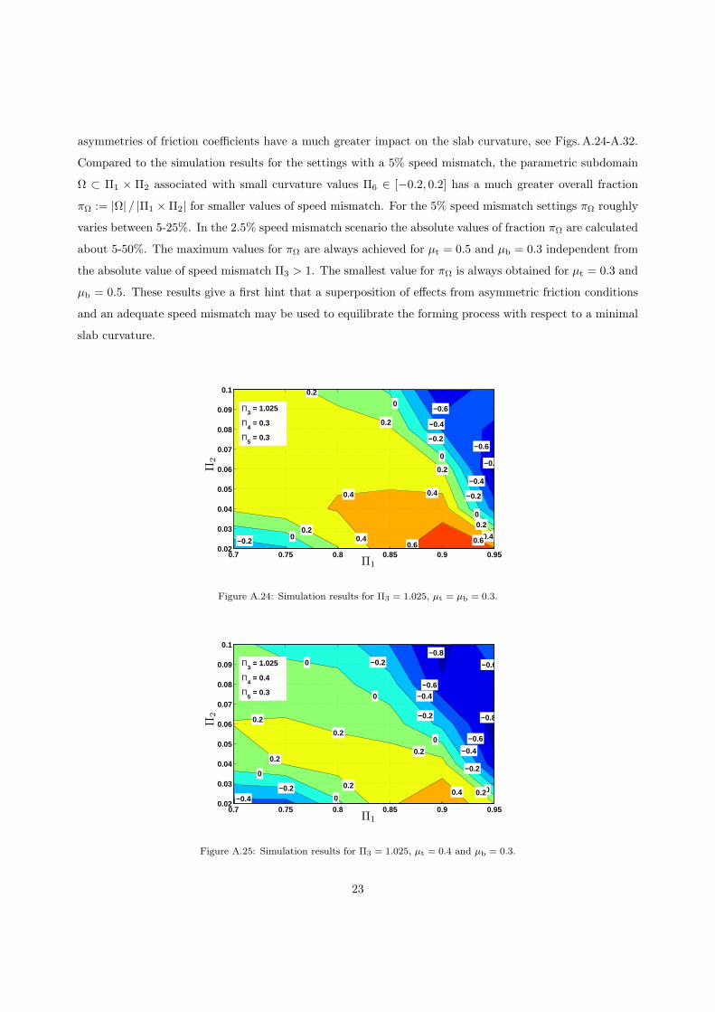
asymmetries of friction coefficients have a much greater impact on the slab curvature, see Figs. A.24-A.32.
Compared to the simulation results for the settings with a 5% speed mismatch, the parametric subdomain
Ω ⊂ Π1 × Π2 associated with small curvature values Π6 ∈ [−0.2, 0.2] has a much greater overall fraction
πΩ := |Ω| / |Π1 ×Π2| for smaller values of speed mismatch. For the 5% speed mismatch settings πΩ roughly
varies between 5-25%. In the 2.5% speed mismatch scenario the absolute values of fraction πΩ are calculated
about 5-50%. The maximum values for πΩ are always achieved for µt = 0.5 and µb = 0.3 independent from
the absolute value of speed mismatch Π3 > 1. The smallest value for πΩ is always obtained for µt = 0.3 and
µb = 0.5. These results give a first hint that a superposition of effects from asymmetric friction conditions
and an adequate speed mismatch may be used to equilibrate the forming process with respect to a minimal
slab curvature.
−0.8
−0.6
−0.6
−0.4
−0.4
−0.2
−0.2
−0.2
0
0
0
0
0.2
0.2
0.2
0.2
0.2
0.4
0.4 0.4
0.40.6
0.6
0.7 0.75 0.8 0.85 0.9 0.950.02
0.03
0.04
0.05
0.06
0.07
0.08
0.09
0.1
Π5 = 0.3
Π4 = 0.3
Π3 = 1.025
Π1
Π2
Figure A.24: Simulation results for Π3 = 1.025, µt = µb = 0.3.
−0.8
−0.8
−0.6
−0.6
−0.4
−0.4
−0.4
−0.2
−0.2
−0.2
−0.2
0
0
0
0
0
00.2
0.2
0.2
0.2
0.2
0.20.4
−0.6
0.7 0.75 0.8 0.85 0.9 0.950.02
0.03
0.04
0.05
0.06
0.07
0.08
0.09
0.1
Π5 = 0.3
Π4 = 0.4
Π3 = 1.025
Π1
Π2
Figure A.25: Simulation results for Π3 = 1.025, µt = 0.4 and µb = 0.3.
23

−0.8
−0.8
−0.8
−0.6
−0.6
−0.6
−0.4
−0.4
−0.4
−0.4−0.2
−0.2
−0.2
−0.2
−0.2
0
0
0
0
0
0
0.2
0.2
0.20.2
−0.6
0.4
0.7 0.75 0.8 0.85 0.9 0.950.02
0.03
0.04
0.05
0.06
0.07
0.08
0.09
0.1
Π5 = 0.3
Π4 = 0.5
Π3 = 1.025
Π1
Π2
Figure A.26: Simulation results for Π3 = 1.025, µt = 0.5 and µb = 0.3.
−0.6
−0.6
−0.4
−0.4
−0.2
−0.2
0
0
0.2
0.2
0.2
0.2
0.4
0.4
0.4
0.4
0.4
0.40.6
0.6
0.7 0.75 0.8 0.85 0.9 0.950.02
0.03
0.04
0.05
0.06
0.07
0.08
0.09
0.1
Π5 = 0.4
Π4 = 0.3
Π3 = 1.025
Π1
Π2
Figure A.27: Simulation results for Π3 = 1.025, µt = 0.3 and µb = 0.4.
−0.8−0.6
−0.6
−0.4
−0.4
−0.4
−0.2
−0.2
−0.2
0
0
0
0
0.2
0.2
0.2
0.2
0.20.4
0.4
−0.6
0.60.7 0.75 0.8 0.85 0.9 0.95
0.02
0.03
0.04
0.05
0.06
0.07
0.08
0.09
0.1
Π5 = 0.4
Π4 = 0.4
Π3 = 1.025
Π1
Π2
Figure A.28: Simulation results for Π3 = 1.025, µt = 0.4 and µb = 0.4.
24
−0.8 −0.8
−0.8
−0.6
−0.6
−0.6
−0.4
−0.4
−0.4
−0.2
−0.2
−0.2
−0.2
0
0
0
0
0
0.2
0.2
0.20.2
0.2
0.20.4
−0.6
0.7 0.75 0.8 0.85 0.9 0.950.02
0.03
0.04
0.05
0.06
0.07
0.08
0.09
0.1
Π5 = 0.4
Π4 = 0.5
Π3 = 1.025
Π1
Π2
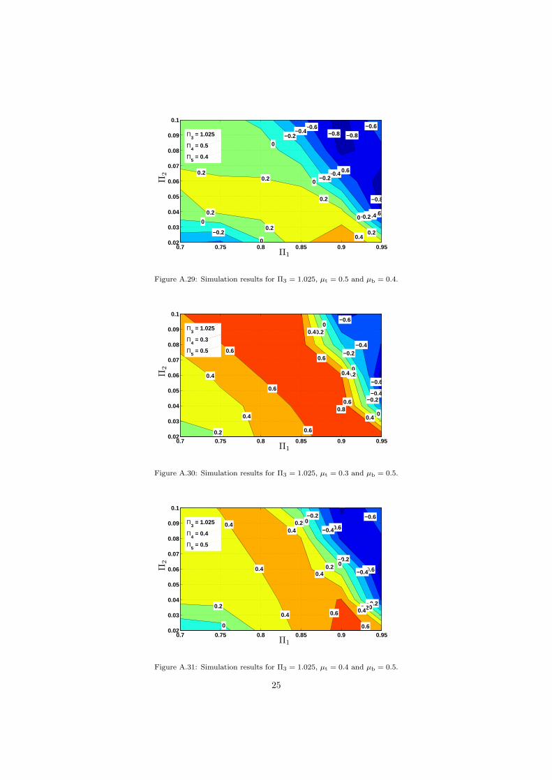
Figure A.29: Simulation results for Π3 = 1.025, µt = 0.5 and µb = 0.4.
−0.6
−0.6
−0.4
−0.4
−0.2
−0.2
0
0
0
0.2
0.2
0.2
0.4
0.4
0.4
0.4
0.4
0.6
0.6
0.60.6
0.60.8
0.7 0.75 0.8 0.85 0.9 0.950.02
0.03
0.04
0.05
0.06
0.07
0.08
0.09
0.1
Π5 = 0.5
Π4 = 0.3
Π3 = 1.025
Π1
Π2
Figure A.30: Simulation results for Π3 = 1.025, µt = 0.3 and µb = 0.5.
−0.6
−0.6
−0.4
−0.4
−0.2
−0.2
−0.2
0
0
0
00.2
0.2
0.2
0.20.4
0.4
0.40.4
0.4
0.40.6
0.6
−0.6
0.7 0.75 0.8 0.85 0.9 0.950.02
0.03
0.04
0.05
0.06
0.07
0.08
0.09
0.1
Π5 = 0.5
Π4 = 0.4
Π3 = 1.025
Π1
Π2
Figure A.31: Simulation results for Π3 = 1.025, µt = 0.4 and µb = 0.5.
25

−0.8 −0.8
−0.8
−0.6
−0.6
−0.4
−0.4
−0.4
−0.2
−0.2
−0.2
−0.2
0
0
0
0
0.2
0.2
0.2
0.2
0.2
0.4
0.4
−0.6
0.7 0.75 0.8 0.85 0.9 0.950.02
0.03
0.04
0.05
0.06
0.07
0.08
0.09
0.1
Π5 = 0.5
Π4 = 0.5
Π3 = 1.025
Π1
Π2
Figure A.32: Simulation results for Π3 = 1.025, µt = 0.5 and µb = 0.5.
26

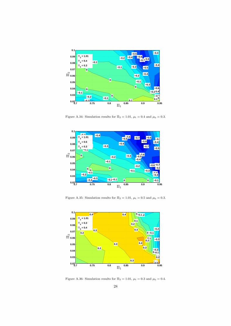
Appendix A.2. Results for 1% speed mismatch
In this section front-end bending events mainly driven by asymmetries in the friction conditions within the
roll gap are considered. Here, the system is subjected to a rather slight speed mismatch of 1%. The obtained
simulation results indicate that this speed mismatch may be employed to compensate certain asymmetric
friction conditions, cf. Figs. A.33-A.41. In this context the values of πΩ have an extremely broad range of 10-
72.5%. Especially the setting with µt = 0.5 and µb = 0.4 where πΩ ≈ 72.5% is of high interest, see Fig. A.38.
In this very configuration the process is almost equilibrated for about 72.5% of the parameter space involving
different geometries of the roll gap. This result corroborates the supposition from the previous section. It
shows that ski effects due to asymmetric friction can be superimposed by slight speed mismatches to achieve
an almost equilibrated rolling process with slight front-end bending.
−0.4
−0.4
−0.3
−0.3
−0.3
−0.2
−0.2
−0.2
−0.1
−0.1
−0.1
0
0
0
0
0.1
0.1
0.1
0.1
0.1
0.10.2
0.2
0.3
−0.2
0.7 0.75 0.8 0.85 0.9 0.950.02
0.03
0.04
0.05
0.06
0.07
0.08
0.09
0.1
Π5 = 0.3
Π4 = 0.3
Π3 = 1.01
Π1
Π2
Figure A.33: Simulation results for Π3 = 1.01, µt = 0.3 and µb = 0.3.
27
−0.6−0.6
−0.6
−0.5
−0.5
−0.4
−0.4
−0.4
−0.3
−0.3
−0.3
−0.2
−0.2
−0.2
−0.2
−0.1
−0.1
−0.1
−0.1
−0.1
−0.10
0
0
0
0
00.1 0.1
−0.4
−0.3
−0.7
0.7 0.75 0.8 0.85 0.9 0.950.02
0.03
0.04
0.05
0.06
0.07
0.08
0.09
0.1
Π5 = 0.3
Π4 = 0.4
Π3 = 1.01
Π1
Π2
Figure A.34: Simulation results for Π3 = 1.01, µt = 0.4 and µb = 0.3.
−0.8
−0.7
−0.7
−0.7
−0.6
−0.6
−0.6
−0.6
−0.5
−0.5
−0.5
−0.4
−0.4
−0.4
−0.4
−0.4−0.3
−0.3
−0.3
−0.3
−0.3
−0.2
−0.2
−0.2
−0.2
−0.2
−0.1
−0.1
−0.1
−0.1
−0.1
−0.1
−0.5
0 00
0 0
−0.4
0
−0.3−0.8
0.7 0.75 0.8 0.85 0.9 0.950.02
0.03
0.04
0.05
0.06
0.07
0.08
0.09
0.1
Π5 = 0.3
Π4 = 0.5
Π3 = 1.01
Π1
Π2
Figure A.35: Simulation results for Π3 = 1.01, µt = 0.5 and µb = 0.3.
−0.3
−0.2
−0.2
−0.2
−0.1
−0.1
−0.1
0
0
0
0.1
0.1
0.1
0.2
0.2
0.2
0.2
0.20.3
0.3
0.3 0.3
0.3
0.4
0.4
0.4 0.4
0.50.7 0.75 0.8 0.85 0.9 0.95
0.02
0.03
0.04
0.05
0.06
0.07
0.08
0.09
0.1
Π5 = 0.4
Π4 = 0.3
Π3 = 1.01
Π1
Π2
Figure A.36: Simulation results for Π3 = 1.01, µt = 0.3 and µb = 0.4.
28

−0.6−0.5
−0.4
−0.4
−0.4
−0.3
−0.3
−0.3
−0.2
−0.2
−0.2
−0.1
−0.1
−0.1
−0.1
0
0
0
0
0.1
0.1
0.1
0.1
0.1
0.1
0.2 0.2
−0.3
−0.5
0.30.7 0.75 0.8 0.85 0.9 0.95
0.02
0.03
0.04
0.05
0.06
0.07
0.08
0.09
0.1
Π5 = 0.4
Π4 = 0.4
Π3 = 1.01
Π1
Π2
Figure A.37: Simulation results for Π3 = 1.01, µt = 0.4 and µb = 0.4.
−0.8
−0.7
−0.6
−0.5
−0.5
−0.5
−0.4
−0.4
−0.4
−0.3
−0.3
−0.3
−0.2
−0.2
−0.2
−0.2
−0.1
−0.1
−0.1
−0.10
0
0
0
0
0
−0.5
0.1
0.1
−0.6
−0.6−0.4
−0.3
−0.7
0.7 0.75 0.8 0.85 0.9 0.950.02
0.03
0.04
0.05
0.06
0.07
0.08
0.09
0.1
Π5 = 0.4
Π4 = 0.5
Π3 = 1.01
Π1
Π2
Figure A.38: Simulation results for Π3 = 1.01, µt = 0.5 and µb = 0.4.
−0.3
−0.2
−0.1
−0.1
0
0
0
0.1
0.1
0.1
0.2
0.2
0.2
0.3
0.3
0.3
0.3
0.3
0.4
0.4
0.4
0.4
0.4
0.4
0.5
0.5
0.5
0.5
0.5
0.5
0.5
0.6
0.6
0.6
0.6
0.2
0.60.7 0.75 0.8 0.85 0.9 0.95
0.02
0.03
0.04
0.05
0.06
0.07
0.08
0.09
0.1
Π5 = 0.5
Π4 = 0.3
Π3 = 1.01
Π1
Π2
Figure A.39: Simulation results for Π3 = 1.01, µt = 0.3 and µb = 0.5.
29

−0.5
−0.4
−0.3
−0.3
−0.3
−0.2
−0.2
−0.2
−0.1
−0.1
−0.1
0
0
00.1
0.1
0.1
0.1
0.2
0.2
0.2
0.2
0.2
0.20.3
0.3
0.3
0.3
0.3
0.3
−0.2
0.40.7 0.75 0.8 0.85 0.9 0.95
0.02
0.03
0.04
0.05
0.06
0.07
0.08
0.09
0.1
Π5 = 0.5
Π4 = 0.4
Π3 = 1.01
Π1
Π2
Figure A.40: Simulation results for Π3 = 1.01, µt = 0.4 and µb = 0.5.
−0.7−0.6−0.5
−0.4
−0.4
−0.4
−0.3
−0.3
−0.3
−0.2
−0.2
−0.2
−0.1
−0.1
−0.1
0
0
0
00.1
0.1
0.10.1
0.1
0.1
−0.4
−0.5
−0.5
0.2
−0.3
−0.6
−0.7
−0.2
0.7 0.75 0.8 0.85 0.9 0.950.02
0.03
0.04
0.05
0.06
0.07
0.08
0.09
0.1
Π5 = 0.5
Π4 = 0.5
Π3 = 1.01
Π1
Π2
Figure A.41: Simulation results for Π3 = 1.01, µt = 0.5 and µb = 0.5.
30