adiﬀuse-interfacemodelforelectrowetting dropsinahele …cjmems.seas.ucla.edu/papers/2007 jfm lu...

J. Fluid Mech. (2007), vol. 590, pp. 411–435. c© 2007 Cambridge University Press

doi:10.1017/S0022112007008154 Printed in the United Kingdom

411

A diffuse-interface model for electrowettingdrops in a Hele-Shaw cell

H.-W. LU1, K.GLASNER2, A. L. BERTOZZI3

AND C.-J. KIM1

1Department of Mechanical and Aerospace Engineering, UCLA, Los Angeles, CA 90095, USA2 Department of Mathematics, University of Arizona, Tucson, AZ 85721, USA

3Department of Mathematics, UCLA, Los Angeles, CA 90095, USA

(Received 22 July 2005 and in revised form 5 July 2007)

Electrowetting has recently been explored as a mechanism for moving small amountsof fluids in confined spaces. We propose a diffuse-interface model for drop motion, dueto electrowetting, in a Hele-Shaw geometry. In the limit of small interface thickness,asymptotic analysis shows that the model is equivalent to Hele-Shaw flow with avoltage-modified Young–Laplace boundary condition on the free surface. We showthat details of the contact angle significantly affect the time scale of motion in themodel. We measure receding and advancing contact angles in the experiments andderive their influence through a reduced-order model. These measurements suggesta range of time scales in the Hele-Shaw model which include those observed in theexperiment. The shape dynamics and topology changes in the model agree well withthe experiment, down to the length scale of the diffuse-interface thickness.

1. IntroductionThe dominance of capillarity as an actuation mechanism at the micro-scale has

received considerable attention. Darhuber & Troian (2005) recently reviewed variousmicrofluidic actuators by manipulation of surface tension. Because of the ease ofelectronic control and low power consumption, electrowetting has become a popularmechanism for microfluidic actuations. The theory of electrowetting and the differentapplications are well-reviewed by Mugele & Baret (2005). Lippman (1875) first studiedelectrocapillary in the context of a mercury-electrolyte interface. The electric doublelayer is treated as a parallel plate capacitor,

γsl (V ) = γsl(0) − 12cV 2, (1.1)

where γsl is the solid–liquid interfacial energy, c is the capacitance per area of theelectric double layer, and V is the voltage across the double layer. The potentialenergy stored in the capacitor is expended in lowering the surface energy. A locallyapplied voltage then creates the surface energy variation to induce drop motion. Kang(2002) calculated the electro-hydrodynamic forces on a conducting liquid wedge on aperfect dielectric, and recovered equation (1.1).

Dielectric breakdown across the electric double layer limits the applicable voltage.Depositing a thin dielectric film (∼ 0.1 µm) using micro-fabrication techniquescommon in micro electromechanical systems (MEMS) prevents such breakdownwithout incurring significant voltage penalty (see Moon et al. 2002), makingelectrowetting-on-dielectric a practical mechanism of micro-scale drop manipulation.

412 H.-W. Lu, K. Glasner, A. L. Bertozzi and C.-J. Kim

+++θ0

---

b

Top substrate

SiO2/Cytop

ElectrodesBottom substrate

Electrodes

Vs

Bottom substrate

Vs

(a) (b)

Cytop

Figure 1. (a) Cross-section of the electrowetting device. (b) Experimental setup for staticcontact angle measurement.

For such a configuration, c in (1.1) represents the capacitance per area of the dielectric.Lee & Kim (1998) demonstrated the first working micro-device driven by electricallycontrolled surface tension with a mercury drop in water. Kim (2000) and Lee et al.(2001, 2002b) subsequently reported handling of water in air. Cho et al. (2001), andPollack, Fair & Shenderov (2000) demonstrated cutting, merging, and transport ofdrops by electrowetting in Hele-Shaw cell geometry. Hayes & Feenstra (2003) utilizedthe same principle to produce a video speed display device.

The electrowetting device we consider is shown in figure 1. The fabrication and theexperimental details will be given in the following section. It consists of a fluid dropconstrained between two solid substrates separated by a distance, b. The aspect ratioof the drop, α = b/R, can be controlled by drop volume and substrate separation.Here we consider experiments where α 0.1. For a constrained drop of radius R

much greater than the drop height b, the geometry approximates a Hele-Shaw cell(see Hele-Shaw 1898), which enjoys a rich history in fluid mechanics (see Saffman1986; Homsy 1987; Bensimon et al. 1986; Howison 1992; Tanveer 2000).

For partially wetting fluids inside a Hele-Shaw cell, surface effects at the contactline can influence the interfacial boundary conditions. Paterson, Fermigier & Limat(1995) and Paterson & Fermigier (1997) experimentally studied the influence of strongsurface defects on the interface of silicon oil and water displacing air in a Hele-Shawcell. Carrillo, Soriano & Ortin (1999, 2000) found that the fingering instability andthe displacement speed of an expanding fluid annulus in a rotating Hele-Shaw cell ishighly sensitive to the wetting condition of the outer interface. Weinstein, Dussan V. &Ungar (1990) theoretically investigated the influence of dynamic contact angles on thesteady-state solutions of viscous fingering in a Hele-Shaw cell. The dynamic contactangle is incorporated into the pressure boundary condition but has only geometricdependence on the steady finger shape. The analysis is specific to a travelling wavesolution and does not directly carry over to the general flow problem in Hele-Shawcell.

Owing to the intense interest in the Hele-Shaw problems, the last ten years hasalso seen the development of numerical methods for solving the Hele-Shaw problem.The boundary integral method developed by Hou, Lowengrub & Shelley (1994) hasbeen quite successful in simulating the long time evolution of free-boundary fluidproblems in a Hele-Shaw cell. However, simulating drops that undergo topologicalchanges remains a complicated, if not ad hoc, process for methods based on sharpinterfaces. Diffuse interface models provide alternative descriptions by defining aphase-field variable that assumes a distinct constant value in each bulk phase. The

Electrowetting in a Hele-Shaw cell 413

material interface is considered as a region of finite width in which the phase-fieldvariable varies rapidly but smoothly from one phase value to another. Such diffuse-interface methods naturally handle topology changes. As we demonstrate in this paper,an energy construction provides a convenient framework in which to incorporate aspatially varying surface energy due to electrowetting. Matched asymptotic expansionsmay be used to demonstrate the equivalence between the diffuse-interface dynamicsand the sharp-interface dynamics in the Hele-Shaw cell.

In this paper we develop a diffuse-interface framework for the study of Hele-Shaw cell drops that undergo topological changes by electrowetting. Using level-setmethods, Walker & Shapiro (2006) considered the unsteady problem of a dropdeformed by a rapidly changing potential distribution. We consider a viscous flowinduced by a steady potential. The related work of Lee, Lowengrub & Goodman(2002a) considered a diffuse interface in the absence of electrowetting in a Hele-Shawcell under the influence of gravity. They used a diffuse-interface model for the chemicalcomposition, coupled to a classical fluid dynamic equation. Our model describes boththe fluid dynamics and the interfacial dynamics through a nonlinear Cahn–Hilliardequation of one phase-field variable. Our approach expands on the work done byGlasner (2003) and is closely related to that of Kohn & Otto (1997) and Otto (1998).

Section 2 describes the experimental setup of drop manipulation usingelectrowetting-on-dielectric. Section 3 describes the sharp-interface fluidic model forthe electrowetting drop in Hele-Shaw cell. We also briefly discuss the role of thecontact line in the context of the sharp-interface model. In § 4, we describe thediffuse-interface model of the problem. Equivalence with the sharp-interface modelwill be accomplished in § 5 through matched asymptotic expansions. Comparisonswill be made in § 6 between the experimental data and the numerical results. To relatethe theoretical prediction to the experimental observation, we construct a reduced-order model in § 7 with constant contact angles similar to the contact angle modelsdiscussed in Saffman (1986), followed by conclusions.

2. Experimental setup2.1. Procedure

The fabrication of electrowetting devices is well documented in Cho, Moon & Kim(2003). Unlike the previous work, we enlarge the device geometry by a factor of 10and use a more viscous fluid such as glycerine to maintain the same Reynolds numberas in the smaller devices. Such a modification allows us to more carefully maintainthe substrate separation and to directly measure the contact angles. The devices arefabricated in the UCLA Nanoelectronics Research Facility. The bottom substrate ispatterned with square metal electrodes of size 1 cm. Two dielectric layers are placedon top of the electrodes, one of Cytop R© fluoropolymer (Asahi Glass, Japan) on top ofa layer of silicon dioxide (SiO2). The top substrate is a cleaved glass with a conductivecoating of indium-tin oxide (ITO). A very thin layer of Cytop R© fluoropolymer thencovers the ITO to increase the surface energy. The thicknesses of the materials used inthe device are summarized in table 1. A drop of fluid with α ∼ 0.1 is dispensed on thebottom substrate. Two solid spacers maintain the substrate separation at ∼ 530 µm(see figure 1a).

If the top substrate is the same as the bottom substrate, the potential drop acrossits dielectric layers will involve the electrical properties of the fluid. To simplify theproblem, we intentionally use only a thin Cytop R© film on the top substrate. It iswell-know that a thin fluoropolymer film is a poor insulator (see Seyrat & Hayes


Material Thickness Dielectric constant

separation height 529 ± 2 µm n/adielectric (SiO2) 498.4 ± 15.5 nm 3.8fluoropolymer(bottom) 245.8 ± 15.5 nm 2.0fluoropolymer(top) 50 nm 2.0

Table 1. Material thicknesses and dielectric constants of an electrowetting device.

2001) so it only affects the charging time across the thick dielectric layers on thebottom substrate. We conduct a set of static experiments using deionized water withsurface tension of 72 dyn cm−1 to confirm this. First, the capacitance per area of theSiO2/Cytop layers on the bottom substrate is characterized by measuring the staticcontact angle of a sessile drop of deionized water under the influence of a varyingvoltage (see figure 1b). Then we cover the drop with the top substrate and repeat theexperiment to characterize the electrowetting effect across the thin Cytop film on thetop substrate.

The glycerine–water mixture with viscosity of 0.020 Pa s, density of 1.28 cm−3, andsurface tension of 67 dyn cm−1 is used for the dynamic experiments. The half-height ofthe cell is an order of magnitude smaller than the capillary length,

√γ /ρg ≈ 2600 µm,

preserving the dominance of surface tension over gravity. To move a drop, part ofthe drop interface must extend over an adjacent electrode. The top substrate and theelectrode below the drop are grounded. Applying a potential on an adjacent electrodemoves the drop to that electrode. The voltage level is varied between 30 V DC and 80V DC. At each voltage level, we move a drop back and forth between two electrodesten times by alternately applying the voltage and ground to each electrode. A dropcan be split by applying potentials on both sides of the drop. A camera is used torecord the motion, from above, at 30 frames per second. Side views of the menisci atthe nose and the tail of a translating drop are recorded at 512 × 256 resolution bya high-speed camera (Vision Research Inc., Wayne, NJ) at 2100 frames per second.The slope of the top substrate is known a priori by focusing on its cleaved edge. Thebottom substrate is assumed to have the same slope. Both surfaces create reflectionsof the menisci allowing us to locate the contact lines. The images are processed byAdobe Photoshop R© and MATLAB R© for edge detection. The capillary numbersof the advancing and receding contact lines are obtained from the side view and thetop view of the drop. Time-indexed images of the translating and splitting drop arecompared to the simulation contours in § 6.

2.2. Statics

Using Young’s equation, we relate the change of contact angle to the electrowettingvoltage,

cos θV − cos θ0 =cV 2

2γlv

, (2.1)

where θV is the static contact angle when we apply a potential, V , on the electrodes.θ0 is the contact angle at zero potential, and γlv is the liquid–vapour surface tension.Figure 2 shows that cos θV linearly increases as a function of V 2, below a criticalvoltage. Above the critical voltage, the contact angle saturates and even decreases. Thisbehaviour is in agreement with previous studies (see Verheijen & Prins 1999; Peykov,Quinn & Ralston 2000; Seyrat & Hayes 2001; Vallet, Vallade & Berge 1999; Shapiro


1000 2000 3000 4000 5000 6000 70000

0.2

0.4

0.6

0.8

1.0

V2

cosθ

V –

cos

θ0

slope = 2.5e – 4(V–2)

Figure 2. cos θV − cos θ0 vs. V 2.

106°

110°

113°

69°

(a) (a)

Figure 3. Static contact angles (±2) of a deionized water drop in an electrowetting device(a) before applying voltage, and (b) after application of 50.18 V.

et al. 2003). The model developed in this work will focus on the voltage level belowthe saturation. The capacitance per area of the SiO2/Cytop layers c =3.6 × 10−5 Fis obtained by multiplying the slope of the linear region with 2γlv . Estimating thisquantity by considering the dielectric layers as two capacitors connected in series (seeMoon et al. 2002) gives a value close to that measured experimentally.

Figure 3 shows the static contact angles of a deionized water drop in anelectrowetting device with a top substrate both with and without an applied voltage.The increase of the top contact angle is of the same order of magnitude as theuncertainty in the measurement. Therefore, we ignore this small increase in our modeland instead focus on the dramatic decrease of the contact angle, by about 40, on thebottom substrate.

2.3. Dynamics

The average velocity of the glycerine–water drop is obtained by dividing the lengthtravelled by the time. Figure 4, inset (a) shows that the drop remains static until athreshold voltage is reached. The threshold voltage to move a glycerine–water dropis approximately 38 V DC. The interface motion remains smooth for voltages upto 65 V DC as shown in figure 4, inset (b). The average velocity of the drop, u,increases linearly with the square of the applied voltage. The typical drop velocity(u ≈ 0.1–1 cm) indicates small scaled Reynolds number, Re∗ =α2 × ρuR/µ ∼ O(10−2).At a higher voltage, we observed pinning on a section of the advancing contact line,causing the drop to form asymmetric shapes such as the one shown in figure 4, inset(c). When moving a drop back and forth between two electrodes using such a highvoltage, each drop movement becomes slower than the previous one. Eventually thedrop stops responding to the applied voltage, suggesting an accumulation of chargestrapped in the dielectric layers.


0 1000 2000 3000 4000 5000 6000

0.1

0.2

0.3

0.4

0.5

0.6

0.7

0.8

V2

Ave

rage

vel

ocit

y (c

m s

–1)

(a) (b) (c)

Figure 4. Average velocity of the drop actuated by electrowetting. Insets show (a) the dropremains motionless at low voltage level (30.2 V DC); (b) the drop advances smoothly at 50.4V DC; (c) asymmetric shape develops due to the pinning of the advancing contact line at 80.0V DC.

Time = 0 ms 1.90 ms 3.81 ms

Time = 7.62 ms 15.7 ms 32.4 ms

Figure 5. Side view of the advancing meniscus of a glycerine–water drop (dark area) at 50.28V DC. The solid white lines depict the orientations of the top and bottom substrates. Aboveand below the white lines are the reflections of the meniscus. The dashed line shows the initialposition of the meniscus.

To fully understand the problem we must also measure the effect of electrowettingon the dynamic contact angles of the drop. A side view of the advancing meniscus isshown in figure 5. The locations of the solid surfaces are depicted by two solid whitelines. A dashed line intersecting the substrates indicates the initial positions of thecontact lines. The onset of electrowetting induces a sudden decrease of the contactangle on the bottom substrate from its static value ≈100, as shown in figure 6. Thecapillary numbers of the contact lines, shown in figure 7, quickly settle down to the


0 10 20 3070

75

80

85

90

95

100

105

110

115

Time (ms)

Adv

anci

ng c

onta

ct a

ngle

(de

g.)

0 20 40 6070

75

80

85

90

95

100

105

110

115

rece

ding

con

tact

ang

le (

deg.

)Time (ms)

θrt ≈ 97 ± 2°

θrt ≈ 95 ± 2°

θb ≈ 72 ± 2°

θt ≈ 111 ± 2°

top

bottom

Figure 6. Evolution of the advancing and receding contact angles of the meniscus in figure 5.

100 102 1040

0.005

0.010

0.015

0.020

Time (ms)

Ca

advancing interface

receding interface

Figure 7. Capillary number of the advancing and receding meniscus.

range of Ca ∼ 10−3. The contact line on the top substrate remains static until anangle of advance ≈ 110 is exceeded. The hysteretic effect causes the initially concavemeniscus to become convex. The contact angles converge toward steady-state valuesafter a short transient time. The steady behaviour of the contact angle is consistentwith the recent numerical finding of Yeo & Chang (2006) for electrowetting films.The direct observation by the camera only reveals the contact angles at two pointsof the curvilinear interface. Along the interface, the capillary number varies withthe normal velocity of the interface. Therefore, we expect the dynamic contact angleto vary along the interface. More advanced experimental techniques are required tocharacterize the evolution of the dynamic contact angle on the entire interface.

3. Sharp-interface descriptionHere we review the classical model of Hele-Shaw fluid dynamics and extend the

model to include electrowetting. For simplicity, we will first neglect the presence of the


contact line. The insight into the fluid dynamics will allow us to construct a simpleleading-order contact line model in § 7.

Consider a viscous drop occupying a space [Ω × b], where b is the height of theHele-Shaw cell. The small value of aspect ratio allows us to employ the lubricationtheory to reduce the momentum equation to Darcy’s law coupled with a continuityequation,

U = − b2

12µ∇P, (3.1)

∇ · U = 0, (3.2)

where U is the depth-averaged velocity, P is the pressure in the drop or the bubble,and µ is the viscosity. Equations (3.1) and (3.2) imply that the pressure is harmonic,P =0.

The interfacial velocity is the fluid velocity normal to the interface, i.e.Un ∼ ∇P |∂Ω · n. The boundary condition for normal stress depends on the interactionsbetween the different dominant forces in the meniscus region. Assuming pressure inthe surrounding fluid is zero:

P |∂Ω = γlv (Aκ0 + Bκ1) ; (3.3)

κ0, defined as 1/r , is the local horizontal curvature and κ1 is defined as 2/b. Differentdynamics and wetting conditions at the meniscus determine the actual curvatures ofthe drop through A and B . In their initial study, Saffman & Taylor (1959) madethe assumptions that A=1 and B = − cos θA where θA is the apparent contact anglemeasured from inside the drop or bubble.

For the incomplete displacement of viscous fluid, Bretherton (1961) showed thatB = 1 +βCa2/3 where β is equal to 3.8 and −1.13 for advancing and recedingmenisci respectively. Park & Homsy (1984) and Reinelt (1987) further showed thatA= π/4+O(Ca2/3). For the special case of a complete displacement by a steady-statefinger as considered by Weinstein et al. (1990), the boundary condition can also beformulated in the form of equation (3.3). In this case, B = − cos(ΘR − σ cosΦ) whereΘR is the angle of recede for the displaced fluid, σ = ∂Θ/∂U is a linear model forthe dynamic contact angle, and Φ is the angle between the outward normal of thesteady-state finger and the velocity U . For a partially wetting drop, we assume thatA= 1, which is supported a posteriori in Appendix B.

When a voltage is applied across an electrode, V (x) = V χ(x), where χ(x) is acharacteristic function of the electrode, Ωw , it locally decreases the solid–liquid surfaceenergy inside the region Ωw

⋂Ω:

γw(V ) = γlv

(− cos θ0 − cV 2

2γlv

), (3.4)

where γw(V ) is the difference between the liquid–solid and the solid–vapour surfaceenergy. In deriving (3.4), we assume that the electrowetting does not affect the solid–vapour surface energy. From the experimental observations, only the dielectric layeron the bottom substrate produces a significant electrowetting effect. Therefore, thesolid–liquid surface energy of a drop in the device is

γdev = γlv

(−2 cos θ0 − cV 2

2γlv

). (3.5)


Ωw

Ωw

p

p1

p2j

i

Ω

Ω

Ωw

θ

∆

Ω

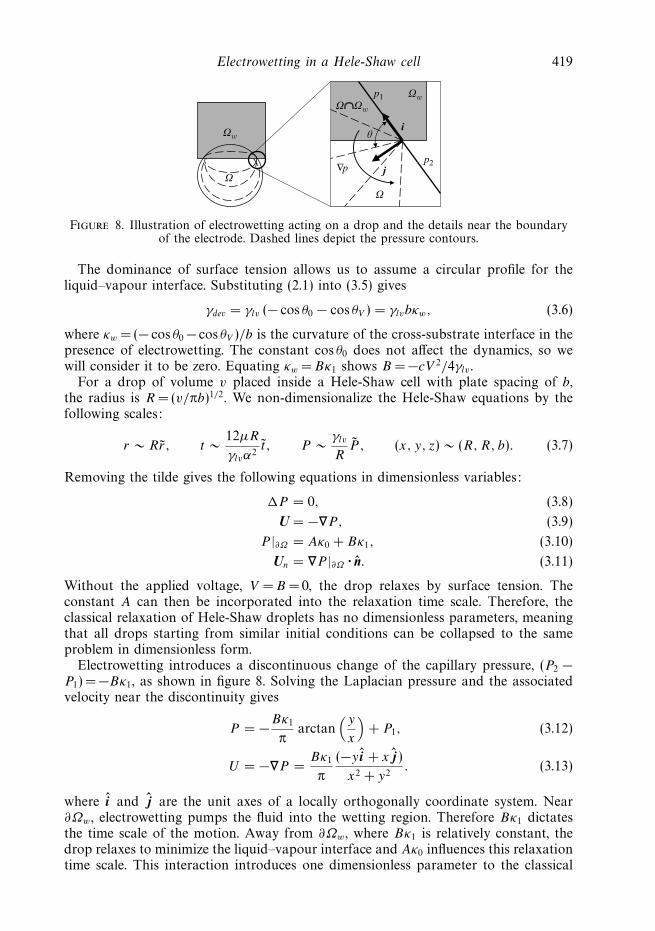
Figure 8. Illustration of electrowetting acting on a drop and the details near the boundaryof the electrode. Dashed lines depict the pressure contours.

The dominance of surface tension allows us to assume a circular profile for theliquid–vapour interface. Substituting (2.1) into (3.5) gives

γdev = γlv (− cos θ0 − cos θV ) = γlvbκw, (3.6)

where κw =(− cos θ0 − cos θV )/b is the curvature of the cross-substrate interface in thepresence of electrowetting. The constant cos θ0 does not affect the dynamics, so wewill consider it to be zero. Equating κw = Bκ1 shows B = −cV 2/4γlv .

For a drop of volume v placed inside a Hele-Shaw cell with plate spacing of b,the radius is R = (v/πb)1/2. We non-dimensionalize the Hele-Shaw equations by thefollowing scales:

r ∼ Rr, t ∼ 12µR

γlvα2t , P ∼ γlv

RP , (x, y, z) ∼ (R, R, b). (3.7)

Removing the tilde gives the following equations in dimensionless variables:

P = 0, (3.8)

U = −∇P, (3.9)

P |∂Ω = Aκ0 + Bκ1, (3.10)

Un = ∇P |∂Ω · n. (3.11)

Without the applied voltage, V = B =0, the drop relaxes by surface tension. Theconstant A can then be incorporated into the relaxation time scale. Therefore, theclassical relaxation of Hele-Shaw droplets has no dimensionless parameters, meaningthat all drops starting from similar initial conditions can be collapsed to the sameproblem in dimensionless form.

Electrowetting introduces a discontinuous change of the capillary pressure, (P2 −P1) = −Bκ1, as shown in figure 8. Solving the Laplacian pressure and the associatedvelocity near the discontinuity gives

P = −Bκ1

πarctan

(y

x

)+ P1, (3.12)

U = −∇P =Bκ1

π

(−y i + x j )x2 + y2

. (3.13)

where i and j are the unit axes of a locally orthogonally coordinate system. Near∂Ωw , electrowetting pumps the fluid into the wetting region. Therefore Bκ1 dictatesthe time scale of the motion. Away from ∂Ωw , where Bκ1 is relatively constant, thedrop relaxes to minimize the liquid–vapour interface and Aκ0 influences this relaxationtime scale. This interaction introduces one dimensionless parameter to the classical


Hele-Shaw flow: we define the electrowetting number

ω = −Bκ1 =cV 2

2αγlv

(3.14)

as the relative measure between the electrowetting potential and the total energy ofthe liquid–vapour interface. This parameter affects both the time scale of motion andthe time scale associated with the drop morphology.

In applying the electrowetting model (3.14) for Bκ1, we assume the contact anglesare determined from a quasi-static balance between the surface energies and theelectrical potential. The presence of moving contact lines introduces deviations fromthe equilibrium values and reduces capillary pressure, Bκ1. In § 7, we will introducethe complication of contact line dynamics through the local dependence of A and B

on the contact angles.

4. Diffuse-interface modelDiffuse-interface (phase-field) models have the advantage of automatically

capturing topological changes such as drop splitting and merger. Here we extendGlasner’s (2003) diffuse-interface model to include electrowetting. The model beginswith a description of the surface energies in terms of a ‘phase’ function ρ thatdescribes the depth average of fluid density in a cell. Therefore ρ =1 corresponds tofluid and ρ = 0 to vapour. Across the material interface, ρ varies smoothly over alength scale ε.

The total energy is given by the functional

E (ρ) =

∫Ω

A

γ

(ε

2|∇ρ|2 +

g (ρ)

ε

)− ρω dx. (4.1)

The first two terms of the energy functional approximate the total liquid–vapoursurface energy

∫∂Ω

γdS where ∂Ω is the curve describing the limiting sharp interface.An interface between liquid and vapour is established through a competition betweenthe interfacial energy associated with |∇ρ|2 and the bulk free energy g(ρ) that hastwo equal minima at ρl and ρv . To avoid the degeneracy in the resulting dynamicmodel (see equations (4.7)–(4.8) and to maintain consistency with the desired sharp-interface limit, we choose ρl =1 and ρv = ε. The final term ρω accounts for the wallenergy (the difference between the solid–liquid and solid–vapour surface energies)on the solid plates. The first two terms act as line energies around the boundaryof the drop while the third term contributes the area energy of the solid–liquidinterfaces.

In equation (4.1), γ is a normalization parameter which we discuss below. Aone-dimensional equilibrium density profile can be obtained by solving the Euler–Lagrange equation of the leading-order energy functional in terms of a scaled spatialcoordinate, z = x/ε,

(ρ0)zz − g′(ρ0) = 0, (4.2)

which has some solution φ(z) independent of ε that approaches the two phases ρl, ρv

as z → ±∞. Integrating equation (4.2) once gives

ε

2φ2

x =g(φ)

ε. (4.3)


Equation (4.3) implies equality between the first and second terms of the energyfunctional so the total liquid–vapour interfacial energy can be written as

γ =

∫ ∞

−∞(φ)2zdz = 2

∫ ∞

−∞g(φ)dz. (4.4)

Equation (4.4) indicates that the choice of g(φ) used to model the bulk free energyinfluences the amount of interfacial energy in the model. Hence this constant appearsas a normalization parameter in the first two terms of the energy functional (4.1).

Since there is no inertia in the physical system, the dynamics take the form of ageneralized gradient flow of the total energy, which can be equivalently characterizedas a balance between energy dissipation and the rate of free energy change,

D ≈∫

R2

ρ|U |2 dxdy. (4.5)

Since ρ is conserved, ρt = −∇ · (ρU). Using this fact and equating the rate of energydissipation to the rate of energy change gives∫

R2

ρ|U |2 dxdy = −∫

R2

ρtδE dxdy = −∫

R2

ρ∇(δE) · U dxdy. (4.6)

To make this true for an arbitrary velocity field U , it follows that U = − ∇(δE).Substituting the velocity back into the continuity gives the evolution of the fluiddensity,

ερt = ∇ · (ρ∇ (δE)) , (4.7)

δE =A

γ(−ε2ρ + g′(ρ)) − εω, (4.8)

subject to boundary conditions that requires no surface energy and no flux at thedomain boundary,

∇ρ · n = 0, (4.9)

ρ∇(δE) · n = 0. (4.10)

Equations (4.7)–(4.8) with ω = 0 constitute a fourth-order Cahn–Hilliard equationwith a degenerate mobility term. By letting ω having spatial dependence, we introduceelectrowetting into the diffuse-interface model.

5. Asymptotic analysisMatched asymptotic expansions show that the sharp-interface limit of the constant-

mobility Cahn–Hilliard equation approximates the two-side Mullins–Sekerka problem(see Caginalp & Fife 1988; Pego 1989). The recent work of Glasner (2003) showed thatthe degenerate Cahn–Hilliard equation approaches the one-sided Hele-Shaw problemin the sharp-interface limit. Using a similar method, we show that the sharp-interfacelimit of the modified Cahn–Hilliard equation (4.7)–(4.8) recovers the Hele-Shawproblem with electrowetting (3.8)–(3.11). The diffuse-interface approximation allowsus to simulate topology changes without artificial surgery of the contour. This isespecially useful as electrowetting devices are designed for the purpose of splitting,merging and mixing of drops.

Using a local orthogonal coordinate system (z, s), where s denotes the distancealong ∂Ω and z denotes signed distance to ∂Ω , r , scaled by 1/ε. The dynamic


equation expressed in the new coordinates is

ε2ρzrt + ε3(ρsst + ρt ) = (ρ( ¯δE)z)z + ερ( ¯δE)zr

+ ε2[ρ( ¯δE)ss + (ρ( ¯δE)s)s |∇s|2],¯δE =

A

γ(−ρzz − ερzr − ε2(ρss |∇s|2 + ρss) + g′(ρ)) − εω

where the denotes the variables in the inner region. The matching conditions are

ρ(0)(z) ∼ ρ(0)(±0), z → ±∞, εz → ±0, (5.1)

ρ(1)(z) ∼ ρ(1)(±0) + ρ(0)r (±0)z, z → ±∞, εz → ±0, (5.2)

ρ(2)(z) ∼ ρ(2)(±0) + ρ(1)r (±0)z + ρ(0)

rr (±0)z2, z → ±∞, εz → ±0. (5.3)

Similar conditions can be derived for ¯δE and δE.The O(1) inner expansion gives(

ρ(0)(

¯δE(0))

z

)z= 0, (5.4)

A

γ

(g′(ρ(0)

)− ρ(0)

zz

)= ¯δE

(0). (5.5)

Equation (5.4) implies (δE)(0) = C(s, t). Equation (5.5) is the equation for the one-dimensional steady state. The common tangent construction implies

¯δE(0)

=γ (g(ρl) − g(ρv))

A(ρl − ρv). (5.6)

The double-well structure of g(ρ) implies ( ¯δE)(0) = 0. At the leading order, thecompetition between interfacial energy and the bulk free energy establishes a stablediffuse interface.

The O(1) outer expansion of (4.7), (4.8) gives

∇ ·(ρ(0)∇g′(ρ(0)

))= 0. (5.7)

The unique solution in the dense phase that satisfies no-flux and matching conditionsis constant, ρ(0) = ρl . Thus on an O(1) scale no motion occurs.

The O(ε) inner expansion results in(ρ(0)

(¯δE

(1))z

)z= 0, (5.8)

A

γ

(g′′ (ρ(0)

)− ∂2

∂z2

)ρ(1) = ¯δE

(1) − A

γκ (0)ρ(0)

z + ω, (5.9)

where the leading-order curvature in the horizontal plane, κ (0), is identified with −r .

Applying matching boundary condition for ¯δE(1)

to equation (5.8) shows that ¯δE(1)

is independent of z; ρ(1) = ρ(0)z is the homogenous solution of (5.9). In the region of

constant ω, the solvability condition gives

ρl

(¯δE

(1))=

Aκ (0)

γ

∫ ∞

−∞

(ρ(0)

z

)2dz − ωρl. (5.10)

The integral is equal to γ , using (4.4). Assuming ρl = 1 and using (3.14) gives

¯δE(1)

=(Aκ (0) + Bκ1

). (5.11)

The surface energy term includes both curvatures of the interface. This is analogousto the Laplace–Young condition of a liquid–vapour interface.


In regions where sharp variation of ω intersects the diffuse interface, the solvabilitycondition becomes

ρl

(¯δE

(1))= Aκ (0) −

∫ ∞

−∞ωρ(0)

z dz. (5.12)

The sharp surface energy variation is smoothly weighted by ρ(0)z , which is O(1) for a

phase function ρ that varies smoothly between 0 and 1 in the scaled coordinate.To order ε, the outer equation in the dense phase must solve

(δE(1)

)= 0, (5.13)

with a no-flux boundary condition in the far field, and a matching condition at theinterface described by (5.2).

The O(ε2) inner expansion reveals the front movement

U (0)n ρ(0)

z =(ρ(0)

(¯δE

(2))z

)z, (5.14)

where rt is identified as the leading-order normal velocity of the interface U (0)n . The

matching condition for ¯δE(2)

gives us the relation for the normal interface velocity ofdrops in a Hele-Shaw cell,

U (0)|n = −(δE(1)

)r. (5.15)

Defining p = δE(1), equations (5.11) (5.13) and (5.15) constitute the sharp-interfaceHele-Shaw flow with electrowetting,

p =0,

p|∂Ω =Aκ (0) + Bκ1,

U (0)n = −(p)r .

⎫⎬⎭ (5.16)

6. Numerical simulations and discussionNumerical methods for solving the nonlinear Cahn–Hilliard equation are an active

area of research. Barrett, Blowey & Garcke (1999) proposed a finite element scheme tosolve the fourth-order equation with degenerate mobility. In addition, the developmentof numerical methods for solving thin-film equations (see Zhornitskaya & Bertozzi2000; Grun & Rumpf 2000; Witelski & Bowen 2003) are also applicable to (4.7)–(4.8).We discretize the equations by finite difference in space with a semi-implicit time step,

ερn+1 − ρn

t+

Aε2M

γ2ρn+1 =

A

γ[ε2∇ · ((M − ρn)∇ρn) + ∇ · (ρn∇g′(ρn))]

− ∇ · (ρnεω). (6.1)

We use a simple polynomial g(ρ) = (ρ − ρv)2(ρ − ρl)

2. The choice of g(ρ) imposesan artificial value of the liquid–vapour surface energy, γ . Integrating (4.4) givesthe normalizing parameter, γ = 0.2322, for the terms associated with the liquid–vapour interface. All numerical results here are computed on a 256 by 128 meshwith x =1/30. The origin is located at the midpoint of the electrode edge thatintersects the drop interface as shown in figure 9. The parameter ε = 0.0427 controlsthe diffuse-interface thickness, which is ∼ 7x for all the results presented here.

A convexity splitting scheme is used where the scalar M is chosen large enoughto improve the numerical stability. We found M = max(ρ) serves this purpose.The equation can be solved efficiently through fast Fourier transform methods.Similar ideas were also used to simulate coarsening in the Cahn–Hilliard equation


y

ycm(t)

R

S1

S2

γ1

γ2

x

Figure 9. Coordinates of the numerical simulation.

0 0.4 0.8 1.2 1.61.0

1.5

2.0

t

Asp

ect r

atio

diffuse interface

boundary integral

–2 –1 0 1 2–2

–1

0

1

2

Figure 10. Aspect ratio of the relaxing elliptic drop calculated by the diffuse-interface model() with ε =0.0427 and boundary integral method ().

(Vollmayr-Lee & Rutenberg 2003) and surface diffusion (Smereka 2003). The diffuse-interface model imposes a constraint on the spatial resolution in order to resolve thetransition layer, x Cε. Preconditioning techniques maybe implemented to relaxthis constraint (see Glasner 2001). We did not employ preconditioning in thisstudy. To ensure the diffuse-interface thickness of the simulation is in the rangerequired by the asymptotic analysis, we performed simulations with smaller valuesof ε on refined meshes and verified that the time scale of motion is independent ofε 0.0427.

We compare the diffuse-interface scheme to the boundary integral method bysimulating the relaxation of an elliptical drop in a Hele-Shaw cell without electro-wetting. Figure 10 shows a close agreement between the aspect ratios of the relaxingelliptic drops calculated by both methods.

To investigate the dynamics of an electrowetting drop without contact linedissipation, we directly compare the diffuse-interface model with A= 1 to theelectrowetting experiments using a glycerine–water drop. The experimental time anddimensions are scaled according to equation (3.7). The dimension of the squareelectrode is 10 cm. The radii of the drops in figures 13 and 14 are approximately0.55 mm and 0.6 mm respectively. Using the capacitance per area, and the surfacetension of the drop reported in § 2, the experimental electrowetting numbers ofωE =7.3 and 8.0 are derived for the drops under 50.4 V DC voltage.


0 0.5 1.0 1.5 2.0–1.0

–0.5

0

0.5

1.0

t

y cm

experimentalω = 7.3ω = 2.7ω = 1.8

Figure 11. Positions of the centre of mass of a moving drop in experiments and insimulations at various electrowetting numbers.

0 0.1 0.2 0.3 0.4 0.5–3

–2

–1

0

1

2

3

Arclength/drop circumference

κ0ω = 7.3ω = 2.7ω = 1.8

Nose Tail

Figure 12. Curvature along the drop contours with ycm = −0.36 from nose to tail.

Figure 11 compares the positions of an experimental drop’s centre of mass, ycm(t),to the simulation results at various ω. Figure 13 below compares the correspondingdrop contours. During the motion, electrowetting creates a necking region of negativecurvature as shown in figure 12. As ω decreases, the variation of the curvature alongthe drop contour decreases due to the increasing influence of the surface tension.When ω = ωE , the motion of the diffuse-interface drop is faster than the experimentby a factor of 2. Scaling the electrowetting number to ω = 3

8ωE matches the simulation

with the experimental motion and produces drop contours that qualitatively agreewith the experiment as shown in figure 13(c).

Figure 14(a) shows the splitting of a drop. The asymmetry of the initial dropplacement yields a difference in size of the daughter drops. Figure 14(b–d) illustratesthe capability of the method to naturally simulate the macroscopic dynamics of dropsplitting. The resolution of the model is limited by the diffuse-interface thickness.Therefore we do not expect the simulation to reproduce the pinch-off of the neckand the formation of satellite drops, as seen in the last few frames of figure 14(a).Electrowetting initially stretches the drop, increasing the capillary pressure in the twoends and decreasing the pressure in the neck. For small ω, the electrowetting cannotovercome the surface tension, which ultimately pumps the entire drop toward the end


(a)

ycm = 0.94 –0.70 –0.36 0.05 0.46 0.73 0.84

(b)

(c)

(d )

Figure 13. Drop movement by electrowetting: (a) experimental images of the drop under50.4 V of potential, (b) diffuse-interface model with ω = 7.3, (c) ω = 2.7, and (d) ω = 1.8. Eachcolumn shows the drop contours with the same centre of mass position.

with smaller curvature as shown in figure 14(d). When ω = ωE , the time scale of dropsplitting is faster in the simulation than in the experiment, by a factor of 8. In thenext section, we show that the contact line dynamics has a significant influence on theelectrowetting number that is more than adequate to account for this discrepancy.

7. Contact line effectThe previous sections investigate the drop dynamics in the absence of additional

contact line effects due to the microscopic physics of the surface (see de Gennes1985). The dynamics near the contact line results in a stress singularity at the contactline (see Huh & Scriven 1971; Dussan V. 1979). Many have studied the contact linedynamics through various mechanisms to regularize the continuum mechanics (seeBerg 1993). Inclusion of van der Waal potential in the diffuse-interface model hasbeen proposed as a regularization of a slowly moving contact line of a partiallywetting fluid (see Pomeau 2002; Pismen & Pomeau 2004).

Implementing a full contact line model for the Hele-Shaw drop requires knowledgeof several microscopic parameters. For viscous fingering in a Hele-Shaw cell, Weinsteinet al. (1990) incorporated a dynamic contact angle model into the capillary pressure.However, their asymptotic analysis relies on a steady-state assumption to avoid


t = 0 0.31 0.64 0.95 1.26 1.58 1.90(a)

t = 0 0.04 0.08 0.12 0.17 0.21 0.25(b)

t = 0 0.3 0.6 0.9 1.2 1.3 1.6(c)

t = 0 0.3 0.6 0.9 1.2 1.5 1.8(d )

Figure 14. Drop splitting by electrowetting: (a) images of a drop pulled apart by twoelectrodes under 50.4 V of potential, (b) diffuse-interface model with ω = 8.0, (c) ω = 3.0,and (d) ω = 2.0.

solving the leading-order velocity in the inner region so the dynamic contact anglemodel only has geometric dependence on the finger shape. Thus their model is notdirectly applicable to our problem in which the interface dynamically changes in time.Therefore, how to consistently incorporate the dynamic contact angle into a generalHele-Shaw flow problem is still an interesting and open problem. Instead we estimatethe influence of the contact line by a reduced-order model with fixed contact angles.Similar contact line models have been used by Ford & Nadim (1994) and Chen et al.


0 2 4 6 8 10–0.8

–0.6

–0.4

–0.2

0

0.2

0.4

0.6

0.8

Time

ycm

t = 0

t = 0.4

t = 0.8

t = 4.0

reduced-order modeldiffuse-interface model

Figure 15. The centres of mass of the reduced-order model and the diffuse-interface model.ε = 0.0427, ω = 5.0.

(2005) in the context of thermally driven drops. Incorporating a fixed contact angleinto the Hele-Shaw model requires a simple extension of the incomplete displacementproblem and was first discussed by Saffman (1986). In Appendix B, we carry outthe necessary asymptotic expansion in the limit of small aspect ratio and extend theformulation to an asymmetric electrowetting meniscus.

The reduced-order approximation considers a drop, in the sharp-interface limit,travelling as a solid circle. This allows us to isolate the time scale of the motion fromthe time scale associated with the shape morphology. In Appendix A, we derive themotion of the circle’s centre of mass, ycm(t), by considering the rate of free energydecrease,

ycm(t) = sin

(−2ω

πt + C

), C = arcsin

ycm(0)

R. (7.1)

Figure 15 compares the centre of mass of the reduced-order model to that of diffuse-interface model. The ability of the diffuse-interface drop to freely deform allows it totranslate slightly faster into the electrowetting region. Once the entire drop mass hasmoved into the wetting region, a slow relaxation toward a circular shape takes place.The close agreement in the translation period shows that the diffuse-interface modeldoes accurately simulate the gradient flow of the energy functional. The discrepanciesof time scale shown in figures 13 and 14 must be attributed to additional effects inthe physical problem.

The deviation of contact angles from their equilibrium values changes the capillarypressure at the interface. The contact angles increase along the advancing contact linesand decrease along the receding contact lines. The capillary pressure difference acrossthe electrowetting and the non-electrowetting regions at the leading order becomes

Bκ1 =(cos θr − cos θt + cos θr − cos θb)

α, (7.2)

where θr is the receding contact angle on the receding contact lines. θt and θb are theadvancing contact angles on the top and the bottom substrates.

In the absence of such deviations, the contact angles assume their equilibriumvalues, and the difference of capillary pressure is represented by the electrowetting


number. Using (3.14) and (2.1) gives

ω = − cV 2

2αγlv

=1

α(cos θ0 − cos θV ). (7.3)

Comparing equations (7.2) and (7.3) gives a scaling factor

ξ =Bκ1

ω=

(cos θs − cos θt ) + (cos θs − cos θb)

cos θ0 − cos θV

, (7.4)

where cos θb < cos θV , cos θt < cos θ0, and cos θr > cos θ0. It can be shown that thescalar ξ is less than 1. The change of the capillary pressure may be incorporated intothe reduced-order model by scaling the electrowetting number accordingly,

ycm(t) = sin

(−2ξω

πt + C

). (7.5)

Substituting the measured values of contact angles from figure 6 gives an estimate ofξ = 0.23. This indicates that the deviation of contact angle may reduce up to 3/4 ofthe capillary pressure difference and account for a four fold increase in the dynamictime scale.

The analysis in § 3 shows that the velocity of the electrowetting drop is proportionalto the difference of Bκ1 across the boundary of the electrowetting region. However,our estimate by the reduced-order model imposes the measured contact angles atthe nose and the tail over the entire electrowetting and non-electrowetting interfaces.Therefore we expect the reduction to 1/4 of the experimental electrowetting numberto yield an upper bound of the time scale increase due to the contact line effect.Figure 13(c, d) shows that reducing ω accordingly in a simulation indeed gives arange of time scale that includes the experimental time scale. The fitting factor for ω

to match the simulated motion with the experiment is ξ =3/8, well within the boundof our estimate. The failure to split the drop as shown in figure 14(d) further confirmsthat the reduction overestimates the contact line effect. The simulation results infigures 13(c) and 14(c) indicate that further refinements with a dynamic contact anglemodel may substantially improve the agreement with the experiment.

8. ConclusionsWe present a diffuse-interface description of the drops in a Hele-Shaw cell in the

form of a degenerate Cahn–Hilliard equation with a spatially varying surface energy.Through matching asymptotic expansions, we show that the phase-field approachapproximates the sharp-interface Hele-Shaw flow in the limit of small diffuse-interfacethickness. The dynamics in the sharp-interface limit is validated numerically by a directcomparison to the boundary integral methods. This approach enables us to naturallysimulate the macroscopic dynamics of drop splitting, merging, and translation underthe influence of local electrowetting.

As illustrated by the reduced-order model, the contact line dynamics significantlyaffects the problem by modifying the cross-substrate of the interface. Based on themeasured advancing and receding contact angles, we showed that the strong influenceof contact line dynamics accounts for up to a four fold increase in the dynamictime scale of the Hele-Shaw approximation. This points out that using the Lippmanequation under the assumption of quasi-steady interfacial motion is not adequateto capture the physics at the interface of the electrowetting drop. Knowledge of theinterface geometries near the electrowetting boundary may improve our estimate.


Numerical simulations of drop motions showed a range of dynamic time scale that isconsistent with the experimentally measured time scale.

The assumption of constant advancing and receding contact angles in the reduced-order model is obviously a crude approximation. Improvements to this approximationneed to account for the dynamically varying contact angle since the normal velocityof the entire drop interface varies. Careful characterizations of the electrowettingcontact line dynamics and asymptotic matching to the bulk Hele-Shaw flow must beconsidered to determine an appropriate pressure boundary condition. In short, this willintroduce velocity dependence in the formulation of B(ω, Ca|∂Ω ) in equation (3.10),where Ca|∂Ω is the local capillary number of the interface. To formulate B(ω, Ca|∂Ω ),the asymptotic analysis of Weinstein et al. (1990) must be extended from the specialcase of a travelling wave solution to the general motion of a Hele-Shaw drop. Doingso presents an interesting problem for future research.

The coupling between pressure boundary condition and the local contact linevelocity can be accomplished by modifying (4.7)–(4.8) to a viscous degenerate Cahn–Hilliard equation (see Seppecher 1996) of the form

ερt + ε2∇ · (ρ∇ f (ρt )) = ∇ · (ρ∇(δE)), (8.1)

δE =A

γ(−ε2ρ + g′(ρ)) − εω, (8.2)

where f (ρt ) is the diffused-interface analogue of the sharp-interface dynamic contactangle model, B(ω, Ca|∂Ω ). The additional nonlinearity in equation (8.1) changes theproperties of the numerical approximation dramatically and warrants new numericalresearch efforts to efficiently solve it. A matched asymptotic expansion similar tothe one in § 5 shows that the addition of f (ρt ) introduces a contact line velocitydependence into the pressure boundary condition.

The threshold voltage for moving a drop shown in figure 4 indicates hysteresis mayalso be a significant source of dissipation. The MEMS fabrication process for theelectrowetting devices produces variations of the surface energy that must be overcomeby the moving contact line. The dissipation becomes more significant as the dropradius decreases, such as in microfluidic applications. Even with the length scale ofour experiment (∼1 cm), the surface effect may become important for specific motionssuch as the splitting of a partially wetting drop. A preliminary study shows the neckwidth at pinch-off is much smaller than the separation height, b. This behaviour isdifferent from experiments mentioned in Constantin et al. (1993), suggesting that thesurface effect may delay the capillary pinch-off by preventing the fluid neck fromseparating off the substrates. For a drop in motion, the linear relationship of thedrop velocity in figure 4 suggests that the dissipation by the contact angle hysteresiscan be accounted for by an offset of the square of the voltage. However, the rangeof linear behaviour is not sufficient to validate this hypothesis. To further study theeffect of hysteresis on the time scale of motion, additional microscopic experimentsare needed to characterize the strength and the uniformity of the defects on thesubstrates. This information will allow us to introduce a macroscopic model of themicroscopic physics, such as the work of Joanny & Robbins (1990), into the study ofelectrowetting drops.

Another interesting problem is that of a viscous drop of larger aspect ratio. Thevelocity component normal to the substrates becomes significant. In this case, thetwo-dimensional Hele-Shaw model can no longer provide an adequate approximation.On the other hand, a fully three-dimensional simulation of such a drop is an extremely


complicated task. It would be desirable to develop a reduced-dimension model that iscomputationally tractable while preserving the essential information about the velocitycomponent normal to the substrates. Galerkin methods from numerical analysis mayprovide an interesting direction to accomplish this.

We thank Pirouz Kavehpour for invaluable experimental support, and discussionson contact line dynamics. We gratefully acknowledge valuable discussions of Hele-Shaw cells with George M. Homsy, and Sam D. Howison. We also thank HamarzAryafar and Kevin Lu for their expertise and assistance in the use of high speedcamera and rheometer. This is work is supported by ONR grant N000140710431,NSF grant CI-0321917, NSF grant DMS-0405596, and NASA through Institute forCell Mimetic for Space Exploration (CMISE).

Appendix A. Reduced-order modelConsider a semi-infinite electrowetting region; we approximate the drop motion as

a moving solid circle. Using the lubrication approximation, we balance the rate ofviscous dissipation with the rate of free energy decrease,

D ≈ − b3

12µ

∫R2

ρ|∇p|2 dxdy = −12µ

b

∫R2

ρ|U |2 dxdy =dE

dt. (A 1)

The centre of the circle travels along the axis as shown in figure 9. The distancebetween the boundary of the electrowetting region and the origin is d . The positionof the centre is y0(t) where y0(0) = 0. The drop moves as a solid circle so the integralreduces to

−12µ|ycm|2πR2

b=

dE

d t, (A 2)

where ycm denotes the velocity of the centre of the circle. The free energy is composedof the surface energy of the dielectric surface with no voltage applied γ1, the surfaceenergy of the electrowetting region γ2, and the liquid-vapor surface energy. Since theliquid-vapor interface area remains constant, the rate of change in free energy is

dE

d t= γ S2, (A 3)

where γ = γ2 − γ1 and S2 is the derivative of the drop area inside the electrifiedregion with respect to time

S2 = −2R2√

1 − y2cmycm. (A 4)

Equations (A 2), (A 3), and (A 4)give the following ODE:

ycm =bγ

6µπR2

√1 − y2

cm. (A 5)

Integrating this ODE we obtain

ycm(t) = sin

(bγ

6µπR2t + C

), C = arcsin

ycm(0)

R, (A 6)

If we neglect the surface effects, the energy difference between the two regionsis well-described by (1.1), γ = −cV 2/2. After changing time to a dimensionless


θs θt

θbθs

z

R

z

r

r′r ′R

(a) (b)

r

Figure 16. Coordinates and geometry of (a) a symmetric interface and (b) an asymmetricinterface due to electrowetting.

0.5 0.6 0.7 0.8 0.9 1.00.5

0.6

0.7

0.8

0.9

1.0

θt/π (rad) θr/π (rad)

A

θb = 0

θb = π/6

θb = π/3

θb = π/2

(a) (b)

0 0.2 0.4 0.6 0.8 1.00.75

0.80

0.85

0.90

0.95

1.00

Figure 17. Horizontal curvature A for (a) electrowetting and (b) non-electrowetting menisci.

variable, we obtain

ycm(t) = sin

(−2ω

πt + C

). (A 7)

Appendix B. Interfacial conditionHere we relate the pressure boundary condition (3.3) to the local contact angle

by perturbation expansions of the governing equations with respect to the aspectratio by considering a radially expanding partially wetting fluid (see Saffman 1986).We calculate the conditions for both the symmetric interfaces and the asymmetricinterfaces. The leading-order expansion then relates the cross-substrate curvature,Bκ1, to the local contact angle, and the next-order expansion corresponds to thecontribution from the horizontal curvature, Aκ0.

Outside the electrowetting region, the interface is symmetric as shown infigure 16(a); z =h(r) gives the shape of the interface. The pressure boundaryconditions are the only relevant equations to solve up to O(α). The equation atthe leading order is integrated twice with boundary conditions h0

r (R) = −∞ andh0(R) = 0 to obtain h0(r) Then apply the boundary conditions that h0(r ′) = 1, wherer ′ =(1 − sin θs)/ cos θs + R to obtain the leading-order pressure. The next order issolved by a similar procedure with the boundary conditions h1

r (R) = 0, h1(R) = 0 andh1(r ′) = 0:

P |∂Ω =−2 cos θs

α− 1 + sin θs

cos θs

(θs

2− π

4

)+ O(α). (B 1)

Inspection of the O(α) term, plotted in figure 17(b), shows that A varies between amaximum of 1 when θs = π/2 and a minimum of π/4 when θs = 0 and π.


If the interface inside the electrowetting region satisfies the requirements thatθt π/2 and θb π/2 as shown in figure 16(b), we can perform similar expansions foran interface inside the electrowetting region with a shifted coordinate. At the leadingorder, we apply the boundary conditions h0

r (R) = − tan θb, h0(R) = 0 and h0(r ′) = 1,where r ′ = −(sin θt − sin θs)/(cos θt + cos θb) + R. The next order is solved with theboundary conditions h1

r (R) = 0, h1(R) = 0 and h1(r ′) = 0:

P |∂Ω =−(cos θb + cos θt )

α− cos θt

2(1 − cos(θb − θt ))

(cos θb

cos θt

sin(θb − θt ) + θt − θb

)+O(α).

(B 2)

Taking the leading-order difference between the two interfaces gives the same formulaas equation (7.2). For the interface inside the electrowetting region, figure 17(a) showsA varying between a maximum value of 1.0 when θb = θt = π/2 and a minimum of0.5 at θb =0 and θt = π/2. Since relaxation dominates away from the boundary of theelectrowetting region, we can obtain good estimate of A by substituting the data infigure 6. The computed values of A are 0.9994 and 0.9831 for the interfaces outsideand inside the electrowetting region respectively. This supports the use of A= 1.

REFERENCES

Barrett, J. W., Blowey, J. F. & Garcke, H. 1999 Finite element approximation of the Cahn–Hilliardequation with degerate mobility. SIAM J. Numer. Anal. 37, 286–318.

Bensimon, D., Kadanoff, L. P., Liang, S. & Shraiman, S. 1986 Viscous flow in two dimensions.Rev. Mod. Phys. 58, 977–999.

Berg, J. C. (Ed.) 1993 Wettability . Marcel Dekker.

Bretherton, F. P. 1961 The motion of long bubble in tubes. J. Fluid Mech. 10, 166–188.

Caginalp, G. & Fife, P. 1988 Dynamics of layered interfaces arising from phase boundaries. SIAMJ. Appl. Maths 48, 506–518.

Carrillo, L., Soriano, J. & Ortin, J. 1999 Radial displacement of a fluid annulus in a rotatingHele-Shaw cell. Phys. Fluids 11, 778–785.

Carrillo, L., Soriano, J. & Ortin, J. 2000 Interfacial instabilities of a fluid annulus in a rotatingHele-Shaw cell. Phys. Fluids 12, 1685–1698.

Chen, J. Z., Troian, S. M., Darhuber, A. A. & Wagner, S. 2005 Effect of contact angle hysteresison thermocapillary droplet actuation. J. Appl. Phys. 97, 014906.

Cho, S. K., Moon, H., Fowler, J., Fan, S.-K. & Kim, C.-J. 2001 Splitting a liquid droplet forelectrowetting-based microfluidics. In Proc. ASME IMECE , Paper. 2001–23831.

Cho, S.-K., Moon, H. & Kim, C.-J. 2003 Creating, transporting, cutting, and merging liquid dropletsby electrowetting-based actuation for digital microfluidic circuits. J. Microelectromech. Syst.12, 70–80.

Constantin, P., Dupont, T. F., Goldstein, R. E., Kadanoff, L. P., Shelley, M. J. & Zhou, S.-M.

1993 Droplet breakup in a model of the Hele-Shaw cell. Phys. Rev. E 47, 4169–4181.

Darhuber, A. & Troian, S. M. 2005 Principles of microfluidic actuation by manipulation of surfacestresses. Annu. Rev. Fluid Mech. 37, 425–455.

de Gennes, P. G. 1985 Wetting: statics and dynamics. Rev. Mod. Phys. 57, 827–863.

Dussan, V. E. B. 1979 On the spreading of liquid on solid surfaces: static and dynamic contactlines. Annu. Rev. Fluid Mech. 11, 371–400.

Ford, M. L. & Nadim, A. 1994 Thermocapillary migration of an attached drop on a solid surface.Phys. Fluids 6, 3183–3185.

Glasner, K. 2001 Nonlinear preconditioning for diffuse interfaces. J. Comput. Phys. 174, 695–711.

Glasner, K. 2003 A diffuse interface approach to Hele-Shaw flow. Nonlinearity 16, 49–66.

Grun, G. & Rumpf, M. 2000 Nonnegativity preserving convergent schemes for the thin filmequation. Numer. Maths 87, 113–152.


Hayes, R. A. & Feenstra, B. J. 2003 Video-speed electronic paper based on electrowetting. Nature425, 383–385.

Hele-Shaw, H. J. S. 1898 The flow of water. Nature 58, 34–36.

Homsy, G. M. 1987 Viscous fingering in porous media. Annu Rev. Fluid Mech. 19, 271–311.

Hou, T., Lowengrub, J. S. & Shelley, M. J. 1994 Removing the stiffness from interfacial flow withsurface-tension. J. Comput. Phys. 114, 312–338.

Howison, S. D. 1992 Complex variable methods in Hele-Shaw moving boundary problems. Eur.J. Appl. Maths 3, 209–224.

Huh, C. & Scriven, L. E. 1971 Hydrodynamic model of steady movement of a solid-liquid-fluidcontact line. J. Colloid Interface Sci. 35, 85–101.

Joanny, J.-F. & Robbins, M. 1990 Motion of a contact line on a heterogenous surface. J. Chem.Phys. 92, 3206–3212.

Kang, K. H. 2002 How electrostatic fields change contact angle in electrowetting. Langmuir 18,10318–10322.

Kim, C.-J. 2000 Microfluidics using the surface tension force in microscale. In SPIE Symp.Micromachining and Microfabrication , vol. 4177, pp. 49–55. Santa Clara, CA.

Kohn, R. V. & Otto, F. 1997 Small surface energy, coarse-graining, and selection of microstructure.Physica D 107, 272–289.

Lee, H., Lowengrub, J. S. & Goodman, J. 2002a Modeling pinchoff and reconnection in a Hele-Shaw cell. I. The models and their calibration. Phys. Fluids 14, 492–513.

Lee, J. & Kim, C.-J. 1998 Liquid micromotor driven by continuous electrowetting. In IEEE MicroElectroMechanical Systems Workshop, pp. 538–543, Heidelberg, Germany.

Lee, J., Moon, H., Fowler, J., Schoellhammer, J. & Kim, C.-J. 2001 Addressable micro liquidhandling by electric control of surface tension. In Proc. IEEE Conf. Micro ElectroMechanicalSystems , pp. 499–502, Interlaken, Switzerland.

Lee, J., Moon, H., Fowler, J., Schoellhammer, J. & Kim, C.-J. 2002b Electrowetting andelectrowetting-on-dielectric for microscale liquid handling. Sensors Actuators A 95, 259–268.

Lippman, M. G. 1875 Relations entre les phenomenes electriques et capillaires. Ann. Chim. Phys. 5,494–548.

Moon, H., Cho, S.-K., Garrel, R. L. & Kim, C.-J. 2002 Low voltage electrowetting-on-dielectric.J. Appl. Phys. 92, 4080–4087.

Mugele, M. & Baret, J.-C. 2005 Electrowetting: from basics to applications. J. Phys.: Condens.Matter 17, R705–R774.

Otto, F. 1998 Dynamics of labyrinthine pattern formation in magnetic fluids: A mean-field theory.Arch. Rat. Mech. Anal. 141, 63–103.

Park, C.-W. & Homsy, G. M. 1984 Two-phase displacement in Hele-Shaw cells: theory. J. FluidMech. 139, 291–308.

Paterson, A. & Fermigier, M. 1997 Wetting on heterogeneous surfaces: Influence of defectinteractions. Phys. Fluids 9, 2210–2216.

Paterson, A., Fermigier, M. & Limat, L. 1995 Wetting on heterogeneous surfaces: Experiments inan imperfect hele-shaw cell. Phys. Rev. E 51, 1291–1298.

Pego, R. L. 1989 Front migration in the nonlinear cahn hilliard equation. Proc. R. Soc. Lond. A422, 261–278.

Peykov, V., Quinn, A. & Ralston, J. 2000 Electrowetting: a model for contact-angle saturation.Colloid Polym. Sci. 278, 789–793.

Pismen, L. M. & Pomeau, Y. 2004 Mobility and interactions of weakly nonwetting droplets. Phys.Fluids 16, 2604–2612.

Pollack, M. G., Fair, R. B. & Shenderov, A. D. 2000 Electrowetting-based actuation of liquiddroplets for microfluidic applications. Appl. Phys. Lett 77, 1725–1726.

Pomeau, Y. 2002 Recent progress in the moving contact line problem: a review. C. R. Mechanique330, 207–222.

Reinelt, D. A. 1987 Interface conditions for two-phase displacement in Hele-Shaw cells. J. FluidMech. 184, 219–234.

Saffman, P. G. 1986 Viscous fingering in Hele-Shaw cells. J. Fluid Mech. 173, 73–94.

Saffman, P. G. & Taylor, G. I. 1959 A note on the motion of bubbles in a Hele-Shaw cell andporous medium. Q. J. Mech. Appl. Maths 12, 265–279.

Seppecher, P. 1996 Moving contact lines in the Cahn-Hilliard theory. Intl J. Engng Sci. 34, 977–992.


Seyrat, E. & Hayes, R. A. 2001 Amorphous fluoropolymers as insulators for reversible low-voltageelectrowetting. J. Appl. Phys. 90, 1383–1386.

Shapiro, B., Moon, H., Garrell, R. L. & Kim, C.-J. 2003 Equilibrium behavior of sessile dropsunder surface tension, applied external fields, and material variations. J. Appl. Phys. 93,5794–5811.

Smereka, P. 2003 Semi-implicit level-set method for curvature and surface diffusion motion. J. Sci.Comput. 19, 439–456.

Tanveer, S. 2000 Surprises in viscous fingering. J. Fluid Mech. 409, 273–308.

Vallet, M., Vallade, M. & Berge, B. 1999 Limiting phenomena for the spreading of water onpolymer films by electrowetting. Eur. Phys. J. B 11, 583–591.

Verheijen, H. J. J. & Prins, M. W. J. 1999 Reversible electrowetting and trapping of charge: modeland experiments. Langmuir 15, 6616–6620.

Vollmayr-Lee, B. P. & Rutenberg, A. D. 2003 Fast and accurate coarsening simulation with anunconditionally stable time step. Phys. Rev. E 68, 066703.

Walker, S. & Shapiro, B. 2006 Modeling the fluid dynamics of electro-wetting on dielectric(EWOD). J. Microelectromech. Syst. 15, 986–1000.

Weinstein, S. J., Dussan, V. E. B. & Ungar, L. H. 1990 A theoratical study of two-phase flowthrough a narrow gap with a moving contact line: viscous fingerin in a Hele-Shaw cell.J. Fluid Mech. 221, 53–76.

Witelski, T. P. & Bowen, M. 2003 Adi schemes for higher-order nonlinear diffusion equations.Appl. Numer. Math. 45, 331–351.

Yeo, L. Y. & Chang, C. H. 2006 Electrowetting films on parallel line electrodes. Phys. Rev. E 73,011605–011616.

Zhornitskaya, L. & Bertozzi, A. L. 2000 Positivity-preserving numerical schemes for lubrication-type equations. SIAM J. Numer. Anal. 37, 523–555.

adiﬀuse-interfacemodelforelectrowetting dropsinahele …cjmems.seas.ucla.edu/papers/2007 jfm lu...

Documents