adjoint-based uncertainty quantification with...
TRANSCRIPT

Adjoint-Based Uncertainty Quantification with MCNP
by
Jeffrey Edwin Seifried
A dissertation submitted in partial satisfactionof the requirements for the degree of
Doctor of Philosophy
in
Engineering - Nuclear Engineering
in the
Graduate Division
of the
University of California, Berkeley
Committee in charge:
Professor Per F Peterson, ChairProfessor Ehud GreenspanProfessor Jasmina L VujicDoctor Jeffery F Latkowski
Professor Van P Carey
Fall 2011

Adjoint-Based Uncertainty Quantification with MCNP
Copyright c© 2011
by
Jeffrey Edwin Seifried

Abstract
Adjoint-Based Uncertainty Quantification with MCNP
by
Jeffrey Edwin Seifried
Doctor of Philosophy in Engineering - Nuclear Engineering
University of California, Berkeley
Professor Per F Peterson, Chair
This work serves to quantify the instantaneous uncertainties in neutron transport sim-ulations born from nuclear data and statistical counting uncertainties. Perturbation andadjoint theories are used to derive implicit sensitivity expressions. These expressions aretransformed into forms that are convenient for construction with MCNP6, creating the abil-ity to perform adjoint-based uncertainty quantification with MCNP6. These new tools areexercised on the depleted-uranium hybrid LIFE blanket, quantifying its sensitivities anduncertainties to important figures of merit. Overall, these uncertainty estimates are small(< 2%). Having quantified the sensitivities and uncertainties, physical understanding of thesystem is gained and some confidence in the simulation is acquired.
Professor Per F Peterson, Chair Date
1

Acknowledgements
Lila Chase for assisting in compiling CRSRD, providing MCNP6 source code and compileadvice, and squashing a strange bug in MAKXSF. John Wagner for providing the source forhis code CRSRD. Massimiliano Fratoni, Antonio Lafuente, Jeff Powers, Tommy Cisneros,Daniel Peters, Alex Hegyi, Tenzing Joshi, Michele Kotiuga, Kevin Kramer, and Ryan Abbottfor helpful discussions. Erin Reeves for patience and understanding. Computing support forthis work came from the Lawrence Livermore National Laboratory (LLNL) InstitutionalComputing Grand Challenge program.
i

“Science is the belief in the ignorance of experts.”—Richard Feynman
ii

Contents
List of Figures v
List of Tables viii
List of Algorithms ix
1 Introduction 11.1 Uncertainty quantification is necessary . . . . . . . . . . . . . . . . . . . . 11.2 Uncertainty quantification has limitations . . . . . . . . . . . . . . . . . . . 31.3 Literature review . . . . . . . . . . . . . . . . . . . . . . . . . . . . . . . . 31.4 Summary of work . . . . . . . . . . . . . . . . . . . . . . . . . . . . . . . . 41.5 Last thoughts . . . . . . . . . . . . . . . . . . . . . . . . . . . . . . . . . . 4
2 Sensitivity and Uncertainty 52.1 Sensitivity-based uncertainty analyses . . . . . . . . . . . . . . . . . . . . . 52.2 Figures of merit and neutronic responses . . . . . . . . . . . . . . . . . . . 62.3 Direct sensitivity and perturbation theory . . . . . . . . . . . . . . . . . . 72.4 Implicit sensitivity . . . . . . . . . . . . . . . . . . . . . . . . . . . . . . . 102.5 Material composition optimization . . . . . . . . . . . . . . . . . . . . . . . 16
3 Sensitivity Estimation with MCNP6 173.1 Constructing the linear functional . . . . . . . . . . . . . . . . . . . . . . . 183.2 Constructing the bilinear functional . . . . . . . . . . . . . . . . . . . . . . 213.3 Editing MCNP6 for elastic scatter tally tagging . . . . . . . . . . . . . . . 453.4 Constructing the adjoint source . . . . . . . . . . . . . . . . . . . . . . . . 453.5 Extracting the importance . . . . . . . . . . . . . . . . . . . . . . . . . . . 533.6 Figure of merit extraction loose ends . . . . . . . . . . . . . . . . . . . . . 553.7 Accounting for Monte Carlo counting uncertainty . . . . . . . . . . . . . . 593.8 Generating a multi-group cross-section library . . . . . . . . . . . . . . . . 663.9 Microscopic cross-section covariance matrices . . . . . . . . . . . . . . . . . 82
iii

4 Sensitivity and Uncertainty in LIFE 854.1 Description of the DU-hybrid LIFE blanket . . . . . . . . . . . . . . . . . . 854.2 Response adjoint source distributions . . . . . . . . . . . . . . . . . . . . . 904.3 Response adjoint/importance distributions . . . . . . . . . . . . . . . . . . 944.4 Sensitivity analysis . . . . . . . . . . . . . . . . . . . . . . . . . . . . . . . 984.5 Validation of adjoint-based methods . . . . . . . . . . . . . . . . . . . . . . 1054.6 Uncertainty analysis . . . . . . . . . . . . . . . . . . . . . . . . . . . . . . . 1064.7 Convergence study (or the lack thereof) . . . . . . . . . . . . . . . . . . . . 118
5 Conclusion 120
Bibliography 122
A Source libraries for nuclear data covariances 130
iv

List of Figures
2.1 An example detector response surrounded by two regions. . . . . . . . . . . . 12
3.1 Spatial dependence of direction within a curve-linear coordinate system. . . . 243.2 Directional smearing for (left) outward- and (right) inward-facing angular bins. 253.3 The region of intersection, broken into four segments for rotation about the z
axis. . . . . . . . . . . . . . . . . . . . . . . . . . . . . . . . . . . . . . . . . 263.4 The five distinct paths for a particle born in a spherical shell until collision. . 373.5 The NJOY99 module sequence for generating multi-group or continuous-energy
ACE-formatted nuclear data and covariances. . . . . . . . . . . . . . . . . . 683.6 Comparison of ENDF70 and ENJEFF flux spectra for natC. . . . . . . . . . 763.7 The natC (left) flux spectrum and (right) radiative capture when the THERMR
module is turned off. . . . . . . . . . . . . . . . . . . . . . . . . . . . . . . . 773.8 The natC (left) absorption and capture cross-sections and (right) flux spectrum
without the egrid and tolmin edits. . . . . . . . . . . . . . . . . . . . . . . 773.9 The 238U flux spectra with (left) 50 energy groups and (right) 150 energy
groups per decade multi-group libraries. . . . . . . . . . . . . . . . . . . . . 783.10 The 238U (left) flux spectrum and (right) radiative capture with the ENJEFF
library. . . . . . . . . . . . . . . . . . . . . . . . . . . . . . . . . . . . . . . . 793.11 The 238U (left) flux spectrum and (right) radiative capture with the ACEJEFF
library. . . . . . . . . . . . . . . . . . . . . . . . . . . . . . . . . . . . . . . . 793.12 The 56Fe flux spectra with (left) 50 energy groups and (right) 150 energy
groups per decade multi-group libraries. . . . . . . . . . . . . . . . . . . . . 803.13 The 56Fe (left) flux spectrum and (right) radiative capture with the ENJEFF
library. . . . . . . . . . . . . . . . . . . . . . . . . . . . . . . . . . . . . . . . 803.14 Comparison of ENDF70 and ENJEFF sensitivity of TBR to 6Li(n,T) reac-
tions for DU-hybrid LIFE at BOL. . . . . . . . . . . . . . . . . . . . . . . . 813.15 The (left) relative uncertainty and (right) correlation matrix for 238U(n, total).
Covariances courtesy of [Shibata et al., 2011; JAEA/NDC, 2011b]. . . . . . . 84
v

4.1 The 6Li cross-section is large at thermal energies and almost exclusively pro-duces tritium. Nuclear data is courtesy of NADS [McKinley et al., 2004]. . . 86
4.2 The 6Li enrichment is adjusted over time for system control. The time-steptitle abbreviations are explained shortly. . . . . . . . . . . . . . . . . . . . . 87
4.3 The LIFE operational parameters behave differently in each of the operationalphases. . . . . . . . . . . . . . . . . . . . . . . . . . . . . . . . . . . . . . . . 88
4.4 The blanket neutron flux spectrum changes strongly during the life-cycle. . . 894.5 The DU-hybrid LIFE engine consists of several functional spherical shell lay-
ers. Figure is courtesy of Morris and Abbott [Abbott et al., 2009]. . . . . . . 904.6 The total adjoint source for (left) TBR and (right) CR are shown over space
and time. . . . . . . . . . . . . . . . . . . . . . . . . . . . . . . . . . . . . . 914.7 The total adjoint source for (left) Mth and (right) Mn are shown over space
and time. . . . . . . . . . . . . . . . . . . . . . . . . . . . . . . . . . . . . . 924.8 The adjoint source distribution is shown for TBR at (left) BOL and (right)
MPU. . . . . . . . . . . . . . . . . . . . . . . . . . . . . . . . . . . . . . . . 924.9 The adjoint source distribution is shown for CR at (left) BOL and (right) MPU. 934.10 The adjoint source distribution is shown at BOL for (left) Mth and (right) Mn. 934.11 The total adjoint/importance is shown for (left) TBR and (right) CR over
space and time. . . . . . . . . . . . . . . . . . . . . . . . . . . . . . . . . . . 944.12 The total adjoint/importance is shown for (left) Mth and (right) Mn over space
and time. . . . . . . . . . . . . . . . . . . . . . . . . . . . . . . . . . . . . . 954.13 The adjoint/importance distribution is shown for TBR at (left) BOL and
(right) MPU. . . . . . . . . . . . . . . . . . . . . . . . . . . . . . . . . . . . 964.14 The adjoint/importance distribution is shown for CR at (left) BOL and (right)
MPU. . . . . . . . . . . . . . . . . . . . . . . . . . . . . . . . . . . . . . . . 974.15 The adjoint/importance distribution is shown at BOL for (left) Mth and (right)
Mn. . . . . . . . . . . . . . . . . . . . . . . . . . . . . . . . . . . . . . . . . . 974.16 The TBR adjoint/importance angular distribution for MPU within (left) the
lithium-lead region and (right) the blanket. Particles with a cosine of positiveone are travelling outwards and particles with a cosine of negative one aretravelling inwards. . . . . . . . . . . . . . . . . . . . . . . . . . . . . . . . . 98
4.17 Comparison of total implicit and explicit sensitivities for (left) TBR at MPIand (right) Mth and EOP. . . . . . . . . . . . . . . . . . . . . . . . . . . . . 99
4.18 Total sensitivities for Mn distributed (left) spatially and (right) isotopically,over time. . . . . . . . . . . . . . . . . . . . . . . . . . . . . . . . . . . . . . 101
4.19 Total sensitivities for (left) Mn and (right) TBR distributed over reaction typeand over time. . . . . . . . . . . . . . . . . . . . . . . . . . . . . . . . . . . . 101
4.20 Total sensitivities for Mth distributed (left) spatially and (right) over reactiontype, over time. . . . . . . . . . . . . . . . . . . . . . . . . . . . . . . . . . . 102
vi

4.21 (Left) positive and (negative) sensitivity energy distributions for TBR at BOLversus isotopic reaction type. . . . . . . . . . . . . . . . . . . . . . . . . . . . 103
4.22 (Left) positive and (negative) sensitivity energy distributions for Mth at MPUversus isotopic reaction type. . . . . . . . . . . . . . . . . . . . . . . . . . . . 103
4.23 Sensitivity energy distributions for TBR at BOP versus spatial region. . . . 1044.24 (Left) positive and (negative) sensitivity energy distributions for Mn at BOP
versus spatial region. . . . . . . . . . . . . . . . . . . . . . . . . . . . . . . . 1044.25 (Left) positive and (negative) sensitivity energy distributions for CR at MPU
versus spatial region. . . . . . . . . . . . . . . . . . . . . . . . . . . . . . . . 1054.26 The 6Li tritium production cross-section has low uncertainty at thermal ener-
gies, but not insignificant uncertainty at high energies. Nominal nuclear datais courtesy of NADS [McKinley et al., 2004]. . . . . . . . . . . . . . . . . . . 112
4.27 The (left) relative uncertainty and (right) correlation matrix for 9Be(n, 2n).Covariances courtesy of [Little et al., 2008; DOE/NNSA, 2011]. . . . . . . . 113
4.28 The (left) relative uncertainty and (right) correlation matrix for 26Fe(n, γ).Covariances courtesy of [Little et al., 2008; DOE/NNSA, 2011]. . . . . . . . 113
4.29 The (left) relative uncertainty and (right) correlation matrix for 2U(n, 3)5fission.Covariances courtesy of [Shibata et al., 2011; JAEA/NDC, 2011b]. . . . . . . 114
4.30 The (left) relative uncertainty and (right) correlation matrix for 238U(n, γ).Covariances courtesy of [Shibata et al., 2011; JAEA/NDC, 2011b]. . . . . . . 114
4.31 Effective intrinsic nuclear data uncertainty is negatively correlated with ex-plicit sensitivity, with a correlation coefficient of -0.071 . . . . . . . . . . . . 115
4.32 Penalty incurred by neglecting a smaller compounding uncertainty. . . . . . 1174.33 Counting uncertainty and counting uncertainty of nuclear data uncertainty
are negatively correlated with explicit sensitivity, with correlation coefficientsof -0.011 and -0.032, respectively. . . . . . . . . . . . . . . . . . . . . . . . . 117
vii

List of Tables
1.1 Estimates of fast reactor simulation uncertainties [Aliberti et al., 2006]. . . . 11.2 Estimates of light-water reactor simulation uncertainties [Weisbin et al., 1982]. 2
3.1 Particle path contributions to directional surface crossing tallies. . . . . . . . 383.2 ENJEFF multi-group energy binning scheme. . . . . . . . . . . . . . . . . . 753.3 Availability of nuclear data covariances circa December 2011. ‡ ENDF/B-
VII.1 is in beta3 and is subject to change before final release. . . . . . . . . . 82
4.1 Top uncertainties of Mth at BOL. . . . . . . . . . . . . . . . . . . . . . . . . 1074.2 Top uncertainties of TBR at BOP. . . . . . . . . . . . . . . . . . . . . . . . 1084.3 Top uncertainties of Mn at MPU. . . . . . . . . . . . . . . . . . . . . . . . . 1094.4 Top uncertainties of CR at EOP. . . . . . . . . . . . . . . . . . . . . . . . . 1104.5 Top uncertainties of TBR at BOT. . . . . . . . . . . . . . . . . . . . . . . . 1114.6 Explicit uncertainties of TBR at BOP. . . . . . . . . . . . . . . . . . . . . . 1114.7 Top ‘diagonal-only’ uncertainties of Mth at BOL. . . . . . . . . . . . . . . . . 116
A.1 Source libraries for nuclear data covariances . . . . . . . . . . . . . . . . . . 139
viii

List of Algorithms
3.1 GetResponseExplicitSensitivitys . . . . . . . . . . . . . . . . . . . . . . . . . 183.2 PopulateSphericalDirectionalMappings . . . . . . . . . . . . . . . . . . . . . 293.3 GetCellAngularDistributionEnergyDistribution . . . . . . . . . . . . . . . . . 343.4 GetCellSourceEnergyAngularDistribution . . . . . . . . . . . . . . . . . . . . 393.5 CalculateResponseImplicitSensitivitys . . . . . . . . . . . . . . . . . . . . . . 413.6 GetCellAdjointSourceEnergyDistribution . . . . . . . . . . . . . . . . . . . . 473.7 WriteAdjointInput . . . . . . . . . . . . . . . . . . . . . . . . . . . . . . . . 483.8 GetCellImportancePerResponseEnergyDistribution . . . . . . . . . . . . . . 543.9 fissileZas . . . . . . . . . . . . . . . . . . . . . . . . . . . . . . . . . . . . . . 553.10 fertileDecayFroms . . . . . . . . . . . . . . . . . . . . . . . . . . . . . . . . . 563.11 Za2FertileParents . . . . . . . . . . . . . . . . . . . . . . . . . . . . . . . . . 563.12 IsZaReactionNumberOfInterest . . . . . . . . . . . . . . . . . . . . . . . . . 573.13 EnergyDistribution . . . . . . . . . . . . . . . . . . . . . . . . . . . . . . . . 60
ix

Chapter 1
Introduction
1.1 Uncertainty quantification is necessary
The purpose of simulation is to make predictions about a system. If the results of thatsimulation are excessively uncertain, they can mislead or bring false meaning to conclusions.A responsible simulation effort quantifies the uncertainties–and therefore limitations–of ananalysis. Monte Carlo neutron transport calculations depend upon many inputs, such asnuclear data, Monte Carlo methods, isotopic number densities, and system geometries. Whenthose inputs are uncertain, the estimates of results we care about–system thermal power, keff ,reactivity feedback coefficients, flux peaking, radioisotope production, material degradation,and others–are also uncertain. Some estimates of simulation uncertainties are shown inTable 1.1 for a generic fast reactor and Table 1.2 for a generic light-water reactor. These
Simulated Result ApproximateUncertainty [%]
Initial keff 0.5Power peaking 3
Power distribution 6Conversion ratio 6
Table 1.1: Estimates of fast reactor simulation uncertainties [Aliberti et al., 2006].
are just some examples of how neutron transport simulation uncertainties can be excessive,and therefore must be quantified.
Nuclear data describe the manner and probability with which nuclei interact with par-ticles. They are predominately generated with experiments that exhibit some experimentaluncertainty and bias and inevitably, experimental estimates of nuclear data do not agreewith each other. A simulator has to decide upon a set of nuclear data values before proceed-
1

Chapter 1. Introduction
Simulated Result ApproximateUncertainty [%]
Power distribution within a fuel pin 8Power distribution axially within an assembly 4-8Power distribution radially among assemblies 2-5
Initial keff 0.3Reactivity during the lifetime 2-6
235U depletion 5Ratio of 239Pu to uranium mass 5
Fissile atoms produced 5
Table 1.2: Estimates of light-water reactor simulation uncertainties [Weisbin et al., 1982].
ing to simulate particle transport. Discrepancies between these chosen values and the ‘true’values exist and many of these are estimated as dispersions that are tabulated alongside theexpected values of nuclear data.
Monte Carlo transport methods sample individual particle histories within a system andaggregate behaviors into expected averages of physical quantity results. The confidence insuch results depends upon the amount of information that is available and relevant to thatbehavior. Mathematically, the coefficient of variation of a result (the standard deviationdivided by the expected value) is equal to the number of instances a particle contributesinformation to the negative one-half power:
cv ≡σ
µ≈ 1√
N, (1.1)
where σ is the standard deviation, µ is the expected value, and N is the number of particleinstances. Therefore, in order to halve the relative uncertainty, the number of particlecontributions to a result must quadruple and by extension four times as many particlehistories must be sampled. These Monte Carlo counting statistics are a prime exampleof aleatory, or random uncertainty, which can be rigorously described with statistics andpropagated in models.
Isotopic densities and system geometries are subject to manufacturing tolerances andchange over the operation of a system. This work quantifies nuclear data and countinguncertainties within Monte Carlo neutron transport models and these sources of uncertaintywere not studied.
2

Chapter 1. Introduction
1.2 Uncertainty quantification has limitations
The scope of a model is limited to the system it considers. Unforeseen and unconsideredphenomena will always lurk outside of the system boundaries. By corollary, an uncertaintyanalysis is limited by the uncertainties it considers–the known unknowns. Such an analysiscannot consider all possible uncertainties, so unknown unknowns will always exist. Whenthere is insufficient information regarding an unknown unknown, predictions or conclusionscannot be safely made. There is a danger of devoting the majority of time and resources tostudying familiar uncertainties, just to build a false sense of security. More effort should bespent searching for new and diverse uncertainties.
1.3 Literature review
There are several groups that perform excellent work in neutron transport uncertainty quan-tification. The SCALE neutronics suite out of Oak Ridge National Laboratory [Team, 2011]contains a package TSUNAMI-3D that calculates sensitivities and uncertainties of nuclearsystems using adjoint-based methods. For the package’s latest update, the breadth of possi-ble analyses expanded from keff sensitivities and uncertainties to generalized perturbations,for which many types of responses can be considered [Jessee et al., 2009; Rearden et al.,2011] TSUNAMI will be quite powerful when contribution theory is full implemented in thecode [Rearden and Williams, 2007; Rearden et al., 2010]. The main advantages this workhas over SCALE are that continuous energy simulations are performed with MCNP6 with noapproximations or corrections like Dancoff factors, multiple-heterogeneity can be modeledfaithfully, transport can be run on distributed parallel systems, and source-driven systemscan be modeled.
Adjoint bilinear functional construction looks to be coming to MCNP6 in the near future[Kiedrowski et al., 2011]. It likely will exist first for keff and critical systems, with eventualextension to general responses and externally sourced systems.
A group out of Seoul National University very thoroughly worked out the theory forpropagating explicit sensitivities through a time-dependent Monte Carlo burnup analysis[Park et al., 2011]. The extension of this from explicit to implicit sensitivities would be ofenormous benefit.
Great work is also performed at NCSU [Abdel-Khalik et al., 2008], but this is essen-tially all direct sampling. A Spanish group went beyond the traditional covariance matrixrepresentation of uncertainties to perturb nuclear data parameters [Garcıa-Herranz et al.,2008].
3

Chapter 1. Introduction
1.4 Summary of work
Chapter 2 of this work describes the mathematics behind sensitivity-based uncertainty anal-yses, outlining its groundings in perturbation theory and adjoint methods. Chapter 3 bringsthe theory of the previous chapter through the painstaking tedium of building methods tocarry out an adjoint-based uncertainty analysis with MCNP6. In Chapter 4, these methodsare put into use, quantifying and studying the sensitivities and uncertainties of the depleted-uranium hybrid LIFE blanket. Lastly, Chapter 5 summarizes the conclusions of the work,identifies its successes and shortcomings, and makes suggestions for future work.
1.5 Last thoughts
Those familiar with the artistic works of Rene Magritte know of his work “The Treachery ofImages” in which an ordinary smoking pipe is depicted. Beneath the pipe, which is paintedas accurately as possible, is written “This is not a pipe” (translated from French). Thereaction of the viewer moves from confusion, to frustration, and finally to resolution withthe fact that Magritte was insane. Upon further reflection, the viewer realizes the deepermessage. The painting is a mere representation, a depiction a smoking pipe, not the realthing. Perhaps nuclear reactor simulations should be mandated to include the statement“This is not a nuclear reactor.”
4

Chapter 2
Sensitivity and Uncertainty
2.1 Sensitivity-based uncertainty analyses
Sensitivity-based uncertainty analyses allow for the propagation of dispersions in a model’sinput data to the uncertainties in differential or integral figure of merit neutronic responses.The process requires just two pieces of information: (1) some quantification of the dispersionof the uncertain inputs; and (2) the sensitivities of figures of merit of interest to those inputdata. Examples of uncertain input data that neutron transport and depletion models aresubject to are nuclear cross-sections for a specific reaction of an isotope within a specific neu-tron energy range, isotopic number densities, and radioactive decay half-lives. The handfulof figures of merit of a design can easily depend upon thousands of uncertain inputs.
While the uncertainty of number densities and half-lives can be represented as scalarvariances, energy-dependent uncertainties of cross-sections are typically tabulated in covari-ance matrices which are generated by the practitioners of nuclear data experiments andcross-section evaluators. Sensitivities to these uncertain inputs–energy-dependent vectorsfor cross-sections and scalars for number densities and half-lives–are problem-specific andrepresent the bulk of the effort in sensitivity-based uncertainty estimation.
Having quantified the relative covariances of each uncertain input C and sensitivitiesof each figure of merit to those inputs S, the uncertainty of that figure of merit U can becomputed as the square root of the linear product of sensitivity and relative covariance inquadratic form:
U =√SCST . (2.1)
In doing so, not only has the confidence in numerical evaluations due to nuclear data uncer-tainties been estimated, but physical insight to the design has also been provided throughsensitivities, and the shortcomings in nuclear data that contribute the most to uncertaintieshave been identified. An uncertainty analysis is always limited to the variety of uncertaintiesthat are considered–neutronic, thermal fluid, and structural simulation uncertainties can be
5

Chapter 2. Sensitivity and Uncertainty
quite unrelated.
2.2 Figures of merit and neutronic responses
Figures of merit are metrics which gauge relative performance of designs and are often pri-mary inputs for design or safety analyses. For neutron transport calculations, figures of meritcan be derived from (or defined as) system neutronic responses such as the thermal power,tritium production, fissile fuel conversion rates, thermal power peaking, neutron leakage,material damage rates, or reactivity. Physically, these all depend upon the neutron flux;mathematically, they can be represented as responses R which are functionals of responseoperators H1,H2, . . . ,Hn and the neutron flux ψ:
R ≡ R[H1,H2, . . . ,Hn, ψ]. (2.2)
Response operators are typically macroscopic cross-sections with spatial-filter delta functionsand the neutron flux is the result of solving the time-independent inhomogeneous neutrontransport equation:
Aψ = S, (2.3)
where A is the transport operator and S is the external neutron source. In this work, Aψ isconsidered the left hand side and S is considered the right hand side of Equation 2.4:
~Ω · ∇ψ(~r, E, ~Ω) + Σt(~r, E) ψ(~r, E, ~Ω)
−∑i
∞∫0
dE ′∫4π
d~Ω′ νxi(E′) Σxi(~r, E
′ → E, ~Ω′ → ~Ω) ψ(~r, E ′, ~Ω′)
= Sex(~r, E, ~Ω),
(2.4)
where νx is the multiplicity of a source reaction: 1 for scattering, νfission for fission, 2 for(n, 2n), 3 for (n, 3n) etc. More details on the neutron transport equation can be found inany of the following texts: [Lewins, 1965; Bell and Glasstone, 1970; Lewis and Miller, 1993;Duderstadt and Hamilton, 1976].
All physical quantities in neutron transport models are distributed over some portion ofthe neutron phase space:
~ξ ≡ (~r, E, ~Ω), (2.5)
where ~r is the spatial coordinate vector, E is the lab-centered neutron kinetic energy, and ~Ωis the neutron direction of travel unit vector. In spherical coordinates,
~Ω ≡ cos(ϕ) sin(θ)~i+ sin(ϕ) sin(θ)~j + cos(θ)~k, (2.6)
6

Chapter 2. Sensitivity and Uncertainty
where ϕ and θ are the azimuthal and zenith angle, respectively. A quantity that is invariantwith all but ~r, either inherently, or after the integration or summation over all other indepen-dent dimensions, can be described as a spatial distribution: the thermal power distributionPth(~r) or the scalar neutron flux distribution φ(~r). A quantity that is invariant with all butE is often referred to as an energy spectrum: the scalar neutron flux spectrum φ(E) or thesensitivity spectrum S(E). Taking the inner product of a quantity ( can represent any
physical quantity) integrates or sums that quantity over all ~ξ:
〈〉 ≡∫~ξ
d~ξ =
∫~r
d~r
∫E
dE
∫~Ω
d~Ω : (2.7)
the total thermal power Pth = 〈Pth(~r)〉 or the total sensitivity S =⟨S(~r, E, ~Ω)
⟩. The inner
product is a linear functional, so it has the mathematical properties of homogeneity:
〈aX〉 = a 〈X〉 , (2.8)
and additivity:〈X + Y 〉 = 〈X〉+ 〈Y 〉 , (2.9)
where X and Y are physical quantities distributed over ~ξ and a is any scalar constant [Renze,2011].
Any response is somewhat dependent upon (sensitive to) an input parameter, but thereis a distinction between explicit and implicit dependence that is important. Explicit de-pendence (explicit sensitivity) exists only when an input directly contributes to a responseby appearing within its response operator H. For example, radiative capture and fissionof plutonium are explicit components of calculating the fissile fuel conversion ratio. How-ever, many nuclear reactions affect ψ (indirectly through Equation 2.3). For example, moststructural materials cannot produce tritium, but still affect tritium breeding as they tendto depress the neutron economy by parasitically absorbing neutrons that might have other-wise bred tritium. Implicit dependence (implicit sensitivity) captures this effect and otherssimilar to it [Greenspan, 1982]. Mathematically, explicit sensitivity constrains the flux andimplicit sensitivity allows it to respond to input perturbations.
2.3 Direct sensitivity and perturbation theory
We define a perturbed quantity that is equal to its nominal value plus a small perturbation:
′ ≡ 0 + δ. (2.10)
7
Chapter 2. Sensitivity and Uncertainty
In a system where an input parameter p that the response depends upon explicitly or im-plicitly is perturbed, the response will also be perturbed. A Taylor expansion can be writtenfor this perturbed response (assuming it is differentiable) with respect to its unperturbedvalue:
R′ = R0 +1
1!
∂
∂pR (p′ − p0) +
1
2!
∂2
∂p2R (p′ − p0)
2+
1
3!
∂3
∂p3R (p′ − p0)
3+ . . . . (2.11)
If either the perturbation in the input parameter is small or the response depends linearlyupon it, a first order approximation is sufficient and the expression can be truncated. Doingso brings about a linear approximation for the response perturbation:
δR = R′ −R0∼=∂R
∂p(p′ − p0) =
∂R
∂pδp. (2.12)
Using the chain rule, the partial derivative in Equation 2.12 can be expanded to the partialdependence of the response upon every term its functional (Equation 2.2) contains:
∂R
∂p=
∂R
∂H1
∂H1
∂p+
∂R
∂H2
∂H2
∂p+ · · ·+ ∂R
∂Hn
∂Hn
∂p+∂R
∂ψ
∂ψ
∂p. (2.13)
Writing the definition of sensitivity as the linear relative change in a response R with respectto a relative perturbation in an input parameter p:
SR,p ≡δR
R
p
δp, (2.14)
it is evident that Equation 2.12 is similar to the sensitivity, modulo a factor of pR
. Multiplyingby this factor, rearranging, and substituting in Equation 2.13 brings about a first orderestimate for the sensitivity of responses of the form of Equation 2.2 to an input parameter:
SR,p ∼=∂R
∂p
p
R=p
R
(∂R
∂H1
∂H1
∂p+
∂R
∂H2
∂H2
∂p+ · · ·+ ∂R
∂Hn
∂Hn
∂p+∂R
∂ψ
∂ψ
∂p
). (2.15)
If the response is a linear functional, consisting of a linear operator (or a linear combi-nation of linear operators) operating on the flux:
R = 〈Hψ〉 , (2.16)
it can be shown that:∂R
∂H= ψ, (2.17)
8

Chapter 2. Sensitivity and Uncertainty
∂R
∂ψ= H. (2.18)
Substituting these into Equation 2.15, the first-order estimate for sensitivity of linear func-tionals becomes:
SR,p ∼=∆HψR
+H∆ψ
R, (2.19)
where the ∆ operator is defined as:
∆ ≡ p∂∂p
. (2.20)
If the response is a ratio of two linear functionals:
R =〈H1ψ〉〈H2ψ〉
, (2.21)
it can be shown that:∂R
∂H1
=ψ
〈H2ψ〉= R
ψ
〈H1ψ〉, (2.22)
∂R
∂H2
= −ψ 〈H1ψ〉〈H2ψ〉2
= −R ψ
〈H2ψ〉, (2.23)
∂R
∂ψ=
H1
〈H2ψ〉− 〈H1ψ〉
(H2
〈H2ψ〉2
)= R
(H1
〈H1ψ〉− H2
〈H2ψ〉
). (2.24)
Substituting these into Equation 2.15, the first-order estimate for sensitivity of ratios oflinear functionals becomes:
SR,p ∼=(
∆H1ψ
〈H1ψ〉− ∆H2ψ
〈H2ψ〉
)+
(H1∆ψ
〈H1ψ〉− H2∆ψ
〈H2ψ〉
). (2.25)
In this section, linear perturbation theory was used to derive expressions for direct sen-sitivities which introduce the ∆ operator (Equation 2.20). This operator effectively filtersout linear operators that explicitly contain the perturbed input parameter p:
∆H ≡ p∂H∂p
=
H, if H contains p0, otherwise.
(2.26)
This operation occurs in the explicit sensitivity terms which make up the first half of thedirect sensitivity expressions. The second half of those expressions are the implicit terms,within which ∆ operates upon ψ. ψ, is not a linear operator; it is the solution of Equation
9

Chapter 2. Sensitivity and Uncertainty
2.3 and can only implicitly depend upon p through its presence in A. Consequently, there isno analytical way to resolve ∆ψ and more sophisticated approaches are necessary.
2.4 Implicit sensitivity
There exist two prominent strategies in side-stepping the implicit term ∆ψ: direct samplingmethods, and adjoint-based methods. In the first, only perturbations are dealt with–inputperturbations and the results of perturbed transport calculations–so ∆ terms are avoided byproducing response sensitivities directly from statistical post-processing. In the second, ∆ψterms are replaced with adjoint bilinear functionals and all uncertain inputs are consideredin parallel with just one or two adjoint calculations per response.
The stark contrast in computational requirements between the two strategies becomesclear when the number of input parameters and responses are compared. A design cancontain hundreds of isotopes, each of which can have just under ten important nuclearreactions that are distributed over just over ten neutron energy decades. Any design containsonly a handful of neutronic responses of interest. An analysis using direct sampling methodsrequires tens of thousands of neutron transport calculations at a minimum while one usingadjoint-based methods requires only a handful. For this work, adjoint-based methods arechosen because of their several order of magnitude advantage in computational expense andfor other reasons which will soon become clear.
2.4.1 Direct sampling methods
In direct sampling methods, an input is directly perturbed a number times and perturbedresponses are extracted from a perturbed transport calculation. A simple linear regressioncan then produce a linear sensitivity for each response to that input. Technically, only oneperturbation is necessary for a linear sensitivity, though more may be desired. Higher-ordersensitivity coefficients can also be generated with polynomial regression, requiring manymore perturbations than for a linear sensitivity.
The following procedure is repeated for every input of concern:
1. A nuclear data parameter is changed a small amount
2. A transport calculation is performed
3. Responses are extracted from results
4. Response sensitivities are calculated
The extreme regularity and repetition of this brute-force method lends itself to automationthrough scripting languages, like Perl, BASH, or Python. For example, MCNP6 is distributed
10

Chapter 2. Sensitivity and Uncertainty
with a Fortran script mcnp pstudy [Brown, 2008] that is marketed for automation of bothparameter studies and random sampling of uncertain parameters in a problem. However,the tool is currently limited to perturbing material densities and the random number seed;dispersions in nuclear data are not addressed. Finally, the straight-forward manner in whichsensitivities (or deviations) can be generated also makes direct sampling methods convenientfor benchmarking of more convoluted methods.
Within an analysis that employs direct sampling methods, there are choices as to howparameters are perturbed. The simplest way is to adjust each parameter by a fractionalamount, one at a time, perhaps positively and negatively. This approach is quite limited inthe sense that it touches only a small part of the entire parameter space and it does so ina very regular way. It effectively assumes that all parameters are independent. Two muchmore effective schemes are Latin Hypercube sampling and orthogonal sampling, for whichit is assured that all regions of phase space are sampled appropriately [Iman and Conover,1982].
2.4.2 Adjoint theory
Historical accounts of the invention of variational methods inevitably mention the brachis-tochrone problem, for which the curve of fastest descent under the acceleration of gravityis sought. In solving this problem, a new field of mathematics, ‘Calculus of Variations,’was born, offering tools to streamline the pursuit and study of extrema and stationarities.Variational methods are used in the fields of mechanics, geometry, economics, control theory,theoretical physics, and others.
In neutronics, variational methods can derive an adjoint neutron transport equation,whose solution, the adjoint neutron flux, is the dual of the forward neutron flux. Solving forone requires no knowledge of the other; both solutions depend upon the system geometryand materials, but the adjoint neutron flux is additionally solved with respect to a defined re-sponse. For each response the resultant adjoint distribution (or importance) is equivalent tothe probability of neutron sources or sinks in regions of neutron phase space in increasing ordecreasing that response, respectively. In other words, the importance quantifies the poten-tial effectiveness of neutrons in causing the response, depending upon where they originatewithin phase space.
For example, consider the neutron flux detector in Figure 2.1 with a neutronic responsedefined as the rate of (n, γ) reactions, surrounded by two optically thin physical regions.If the response importance of region A is twice that of region B, neutrons that are bornin region A are twice as likely to contribute to the response. Contrariwise, neutrons lost inregion B are half as likely to diminish the (n, γ) reading on the detector as those lost in regionA. Synthesizing, neutron source and sink perturbations in region A are twice as significantin perturbing the detector reading as neutron source and sink perturbations in region B.The adjoint distribution enables one to quantify the implicit effect that perturbations have
11

Chapter 2. Sensitivity and Uncertainty
Region A Region B
Detector
Figure 2.1: An example detector response surrounded by two regions.
on a response, by way of their influence upon the flux [Selengut, 1959; Lewins, 1965; Stacey,1974; Greenspan, 1976a; Coveyou et al., 1967].
In the next section, the variational method of Lagrange multipliers is used to derive theadjoint neutron transport equation for a neutronic response. The solution of this equationproduces the adjoint distribution, or importance. The powerful ability of the adjoint tosimplify expressions containing ∆ψ terms is then demonstrated using this variational methodand a differential method [Williams, 1982].
2.4.2.1 Derivation with variational methods
A Lagrange functional L can be written for a response functional R, using the forward time-independent inhomogeneous neutron transport equation (Equation 2.3) as a constraint andLagrange multiplier λ:
L ≡ R− 〈λ(Aψ − S)〉 . (2.27)
The functional is nominally equal to the response due to nominal satisfaction of the constraintand can be considered explicitly dependent only upon the Lagrange multiplier, the neutronflux, and the transport operator which will be represented by an arbitrary input parameterp:
L = L[λ, ψ, p] = R. (2.28)
Similarly, upon perturbation of the input parameter, a perturbed functional can be writ-ten:
L′ = L[λ′, ψ′, p′] = R′. (2.29)
A Taylor expansion (terminating at first order) can be written for the perturbed functional
12

Chapter 2. Sensitivity and Uncertainty
with respect to the unperturbed functional:
L′ ∼= L+
⟨∂L
∂λδλ+
∂L
∂ψδψ +
∂L
∂pδp
⟩. (2.30)
Combining the three previous equations, the first variation in the response functional isfound:
δR ≡ R′ −R0∼=⟨∂L
∂pδp
⟩∣∣∣∣λ,ψ
+
⟨∂L
∂λδλ
⟩∣∣∣∣p,ψ
+
⟨∂L
∂ψδψ
⟩∣∣∣∣p,λ
. (2.31)
If the first variation of the response functional is stationary about the Lagrange multiplierand flux (i.e. if the last two terms in Equation 2.31 are zero), it can simplify to onlythose terms that explicitly depend upon the perturbation. Stationarity about the Lagrangemultiplier requires: ⟨
∂L
∂λδλ
⟩∣∣∣∣p,ψ
= 〈(Aψ − S)δλ〉 = 0, (2.32)
or for an arbitrary δλ:Aψ − S = 0, (2.33)
which is satisfied by Equation 2.3. Stationarity about the neutron flux requires:⟨∂L
∂ψδψ
⟩∣∣∣∣p,λ
=
⟨∂R
∂ψδψ
⟩− 〈λAδψ〉 = 0, (2.34)
or applying the commutativity relation of an adjoint operator 〈x,By〉 =⟨y,B†x
⟩[Weisstein,
2011a]: ⟨(∂R
∂ψ− A†λ
)δψ
⟩= 0, (2.35)
or for an arbitrary δψ:
A†λ =∂R
∂ψ. (2.36)
This equation has the same form as the forward time-independent inhomogeneous neutrontransport equation (Equation 2.3), with the adjoint of the transport operator A† in place ofthe forward transport operator, the Lagrange multiplier (hereafter referred to as the adjointflux ψ†) in place of the neutron flux, and a response partial derivative (hereafter referred toas the adjoint source S†) in place of the forward external neutron source. Stationarity of theresponse functional about the neutron flux requires that the adjoint flux satisfy the adjointtime-independent inhomogeneous neutron transport equation:
A†ψ† =∂R
∂ψ≡ S†. (2.37)
13

Chapter 2. Sensitivity and Uncertainty
In this work, A†ψ† is considered the left hand side and S† is considered the right hand sideof Equation 2.38:
−~Ω · ∇ψ†(~r, E, ~Ω) + Σt(~r, E) ψ†(~r, E, ~Ω)
−∑i
νxi(E)
∫4π
d~Ω′∞∫
0
dE ′ Σxi(~r, E → E ′, ~Ω→ ~Ω′) ψ†(~r, E ′, ~Ω′)
= Sex(~r, E, ~Ω).
(2.38)
All terms are consistent with their representation in Equation 2.4. More details on thetransport equation can be found in any of the following texts: [Greenspan, 1976b; Lewis andMiller, 1993].
With a neutron flux that satisfies Equation 2.3 and an adjoint flux that satisfies Equation2.37, the Lagrange functional is stationary about all but p (the first term in Equation 2.31):
δR ∼=⟨∂L
∂pδp
⟩∣∣∣∣λ,ψ
=
⟨(∂R
∂p
∣∣∣∣ψ
− ψ†∂A∂p
ψ + ψ†∂S∂p
)δp
⟩, (2.39)
or using Equation 2.13:
δR ∼=⟨∂R
∂pδp
⟩−⟨(
∂R
∂ψ
∂ψ
∂p−(−ψ†∂A
∂pψ + ψ†
∂S∂p
))δp
⟩. (2.40)
When this equation is compared to Equation 2.12, it is clear that the second term is zero,or for arbitrary δp:
∂R
∂ψ
∂ψ
∂p= −ψ†∂A
∂pψ + ψ†
∂S∂p. (2.41)
This relation allows for the elimination of ∆ψ by substituting in more manageable terms inwhich ∆ is operating only upon linear operators. In the next section, this relation is derivedusing differential methods.
2.4.2.2 Derivation with differential methods
Writing the forward time-independent inhomogeneous neutron transport equation (Equation2.3) for a perturbed system:
(A + δA)(ψ + δψ) = S + δS, (2.42)
the unperturbed terms can be eliminated with Equation 2.3 and the second-order perturba-tion terms can be neglected:
Aδψ = −δAψ + δS. (2.43)
14

Chapter 2. Sensitivity and Uncertainty
Subtracting the inner product of the flux perturbation δψ with Equation 2.37 from theinner product of the adjoint flux ψ† with Equation 2.43:
⟨ψ†,Aδψ
⟩−⟨δψ,A†ψ†
⟩= −
⟨ψ†, δAψ
⟩+⟨ψ†δS
⟩−⟨∂R
∂ψδψ
⟩. (2.44)
Applying the commutativity relation of an adjoint operator 〈x,By〉 =⟨y,B†x
⟩, the first two
terms can be canceled: ⟨∂R
∂ψδψ
⟩= −
⟨ψ†, δAψ
⟩+⟨ψ†δS
⟩. (2.45)
When perturbations are truncated to first order like in Equation 2.12, Equation 2.41 emerges,showing that the variational and differential derivations are equivalent.
2.4.2.3 Adjoint-based sensitivity
Taking advantage of the tranformative properties of the adjoint flux exemplified in Equation2.41, a new first-order adjoint-based sensitivity for responses with the form of Equation 2.2is found to replace the direct version of Equation 2.15:
SR,p ∼=∂R∂H1
∆H1
R+
∂R∂H2
∆H2
R+ · · ·+
∂R∂Hn
∆Hn
R− ψ†∆Aψ
R+ψ†∆SR
. (2.46)
For linear functional responses with the form of Equation 2.16, the first-order estimate forsensitivity becomes:
SR,p ∼=(
∆Hψ〈Hψ〉
)− ψ†∆Aψ
R+ψ†∆SR
, (2.47)
with adjoint source:
S† = H =
(R
〈Hψ〉
)H. (2.48)
For ratios of linear functional responses with the form of Equation 2.21, the first-orderestimate for sensitivity becomes:
SR,p ∼=(
∆H1ψ
〈H1ψ〉− ∆H2ψ
〈H2ψ〉
)− ψ†∆Aψ
R+ψ†∆SR
, (2.49)
with adjoint source:
S† = R
(H1
〈H1ψ〉− H2
〈H2ψ〉
)=
(R
〈H1ψ〉
)H1 −
(R
〈H2ψ〉
)H2. (2.50)
15

Chapter 2. Sensitivity and Uncertainty
With the adjoint flux and an ∆A that can be expressed analytically, the implicit effectsof any and all input perturbations can be quantified with respect to a nominal state withoutever having to calculate a single perturbed state or ∆ψ.
2.5 Material composition optimization
The utility of sensitivities is not limited to propagating uncertainties; they can also be atool for optimization. If the input parameter p is the atomic density of an isotope, thetotal sensitivity of a response R to that input parameter SR,p quantifies the linear effect ofchanges in that isotope’s density upon the response. If this sensitivity is positive, incrementsor decrements in the density will increase or decrease the response, respectively. Negativesensitivities indicate the opposite and responses are essentially independent of (insensitiveto) the density if this sensitivity is small or zero. If extremal responses are desired, isotopicdensity adjustments can be performed iteratively with sensitivity estimations until all sensi-tivities are small. This can be especially effective when isotopic densities and sensitivities aredistributed spatially. Physical insight can also be garnered from the sensitivity distribution[Greenspan, 1982; Cacuci, 2003].
Because of properties of the ∆ operator described in Equation 2.26, when p is an isotopicatomic density, ∆ hits all source and sink cross-sections for that isotope. Additionally, due totheir relative senses, sensitivities to macroscopic and microscopic cross-sections are identical.Consequently, the sensitivity of a response to an isotopic atomic density is equivalent to thesum of the sensitivities of that response to the cross-sections (macroscopic or microscopic)for that isotope of every reaction type:
SR,z =∑i
SR,zxi , (2.51)
where z and xi denote the isotope index and reaction type index, respectively. Often isotopicdensity optimization is not possible because the isotopes of interest are contained within asingle element or chemical compound. In these cases, the individual isotopic sensitivitiesmust be combined according to their relative atomic abundances within the material:
SR,m =
∑i aiSR,zi∑
i ai, (2.52)
where m and ai denote the material index and the atomic abundances, respectively.
16
Chapter 3
Sensitivity Estimation with MCNP6
In Chapter 2, adjoint-based sensitivities were derived for two types of responses: (1) linearfunctionals of the flux; and (2) ratios of linear functionals of the flux. Ultimately, the termsnecessary to construct these sensitivities must be extracted from neutron transport simula-tions. This chapter describes that process for the three-dimensional, continuous energy, trueheterogeneous, Monte Carlo neutron transport code MCNP6 [X-5 Monte Carlo Team, 2005].Upon inspection, three types of terms emerge within these sensitivities (Equations 2.47 and2.49): (1) response operator linear functionals ∆Hψ (or equivalently Hψ); (2) transport op-erator bilinear functionals ψ†∆Aψ; and (3) source perturbation linear functionals ψ†∆S. Inthe absence of source perturbations in this work, source perturbation linear functionals arezero and consequently are ignored. The remaining two terms are addressed in turn.
Explicit sensitivity (for which implicit terms are neglected) requires just the constructionof response operator linear functionals. Implicit sensitivity extraction is quite a bit moreinvolved since it additionally requires construction of the transport operator bilinear func-tionals, which are difficult to extract. Each of the necessary steps is described in the sectiondedicated to construction of the transport operator bilinear functional. First, it is expandedinto more manageable terms, introducing the angular distribution. After the angular distri-bution is studied in depth and discretized, angle smearing is solved for curve-linear sphericalcoordinate systems. Neutron sinks and sources are then discretized using tally tags andall the pieces are assembled to calculate implicit sensitivities. Source code is provided foralgorithms when it is appropriate.
Afterwards, a patch is described, which enables MCNP6 to tally source distributionsfor particles ‘born’ from elastic scatters. Then, proper construction of adjoint sources andsubsequent tallying of adjoint distributions is shown. Proper extraction of figure of meritresponses and propagation of counting uncertainties onto nuclear data uncertainties are thendiscussed. Finally, generation of multi-group cross-section libraries for adjoint transportcalculations and nuclear data covariances are described.
17

Chapter 3. Sensitivity Estimation with MCNP6
3.1 Constructing the linear functional
When H is a macroscopic cross-section, ∆Hψ is a reaction rate distribution, shown here asdistributed over (~r, E) in neutron phase space:
∆Hψ ≡∫~Ω
d~Ω p∂H∂p
(~r, E) ψ(~r, E, ~Ω)
=
∫~Ω
d~Ω Σz,x(~r, E) ψ(~r, E, ~Ω)
= Σz,x(~r, E)
∫~Ω
d~Ω ψ(~r, E, ~Ω)
= Σz,x(~r, E) φ(~r, E)
= Rz,x(~r, E),
(3.1)
where z and x are the indices for the isotope and reaction type of input parameter p,respectively. In a discrete sense, this can be extracted directly from MCNP6 with a standardFM4 cell flux multiplier tally for multiple cells, binned over neutron energy [X-5 Monte CarloTeam, 2005, p. 2-105]:
∆Hψ = FM4c,z,x(E), (3.2)
where c is the cell index of input parameter p. The values of the linear functional withineach cell and energy bin (per unit bin width) are effective averages for those discrete regionsin phase space, which converge to the true continuous values as the bin size is shrunk toarbitrarily small size. The collapse over ~ξ is not affected by binning scheme and subsequently,there are no discretization errors in the evaluation of the total linear functional 〈∆Hψ〉 withFM4 tallies.
The algorithm for extracting explicit sensitivities for a given response iterates over all FM4
cell flux multiplier tallies within a forward MCNP6 calculation, finding those that match withconstituents of the response and adjusting for the required multiplicity and sign. Dependingon the purpose of the sensitivity, it can be accumulated over cells, isotopes, reactions, orcombinations thereof, for possible indices of (c, z, x), (c, z), (z, x), and (z). The results arethen divided by the total linear functional and multiplied by the response, consistent withthe explicit sensitivity expressions for both types of responses (see Equations 2.47 and 2.49).Specific details of the algorithm can be found in the GetResponseExplicitSensitivitys
method of the McnpOutputFile class within ParseMcnp.py:
Algorithm 3.1: GetResponseExplicitSensitivitys1 def G e t R e s p o n s e E x p l i c i t S e n s i t i v i t y s ( s e l f , response , sumOverCells , sumOverZas ,
sumOverReactions ) :
18

Chapter 3. Sensitivity Estimation with MCNP6
2 ###3 a s s e r t ( s e l f . GetIsForward ( ) ) ;4 ###5 # Total d iv idend and d i v i s o r6 ###7 t o t a l s = ( s e l f . GetTotal ( r e sponse . GetDividend ( ) ) , s e l f . GetTotal ( r e sponse .
GetDivisor ( ) ) ) ;8 ###9 # Perturba t ion
10 ###11 per turbat i on = response . GetPerturbat ion ( ) ;12 i s P e r t u r b a t i o n = bool ( pe r turbat i on ) ;13 i f i s P e r t u r b a t i o n :14 perturbCellNumber , perturbZa , perturbReactionNumber = per turbat i on [ 0 ] ;15 ###16 # I t e r a t e over reac t i on ra te t a l l y s17 ###18 k e y 2 E x p l i c i t S e n s i t i v i t y = ;19 for cellNumber , m u l t i p l i e r B i n s in s e l f . GetTa l ly Ind i ce s ( ’ fm4 ’ ) . i tems ( ) :20 ###21 # Kick out immateria l c e l l s22 # Only c e l l s wi th mate r ia l s can con t r i bu t e to e x p l i c i t s e n s i t i v i t y23 ###24 i f not s e l f . F indCel l ( cellNumber ) . GetMaterialNumber ( ) :25 continue ;26 ###27 # I t e r a t e over mu l t i p l i e r b ins28 ###29 for materialNumber , reactionNumber in m u l t i p l i e r B i n s :30 try :31 ###32 # Extract s i n g l e−za from mater ia l number33 ###34 za = s e l f . GetMaterialNumber2SingleZa ( ) [ materialNumber ] ;35 except KeyError :36 ###37 # Kick out non−s i n g l e−za mater ia l numbers38 ###39 continue ;40 ###41 # Kick out i f i nd i c e s don ’ t match pe r tu rba t i on ind i c e s42 ###43 i f i s P e r t u r b a t i o n :44 # c45 i f perturbCellNumber not in (None , cellNumber ) :46 continue ;47 # z48 i f perturbZa not in (None , za ) :49 continue ;50 # x51 i f perturbReactionNumber not in (None , reactionNumber ) :52 continue ;53 ###54 # Extract mu l t i p l i c i t y s o f ( c e l l number , mater ia l number , r eac t i on
number ) wi th in response55 ###56 m u l t i p l i c i t y s = response . G e t M u l t i p l i c i t i e s ( cellNumber , materialNumber ,
reactionNumber ) ;57 ###58 # I t e r a t e over div idend , d i v i s o r
19

Chapter 3. Sensitivity Estimation with MCNP6
59 ###60 for index in range (2 ) :61 m u l t i p l i c i t y = m u l t i p l i c i t y s [ index ] ;62 ###63 # Kick out ( c e l l number , mater ia l number , r eac t i on number ) with
nu l l m u l t i p l i c i t y64 ###65 i f not m u l t i p l i c i t y :66 continue ;67 ###68 # Exp l i c i t s e n s i t i v i t y d i s t r i b u t i o n69 ###70 e x p l i c i t S e n s i t i v i t y = SafeDiv ide ( s e l f .
GetCel lReact ionRateEnergyDistr ibut ion ( cellNumber ,materialNumber , reactionNumber ) , t o t a l s [ index ] / m u l t i p l i c i t y );
71 ###72 # Square away summation ind i c e s73 ###74 key = [ ] ;75 ###76 i f not sumOverCells :77 ###78 # Ascend to root c e l l79 ###80 for c e l l in s e l f . FindRootCel ls ( cellNumber ) :81 cellNumber = c e l l . GetNumber ( ) ;82 break ;83 key . append ( cellNumber ) ;84 ###85 i f not sumOverZas :86 key . append ( za ) ;87 ###88 i f not sumOverReactions :89 key . append ( reactionNumber ) ;90 ###91 key = tup l e ( key ) ;92 ###93 try :94 k e y 2 E x p l i c i t S e n s i t i v i t y [ key ] += e x p l i c i t S e n s i t i v i t y ;95 except KeyError :96 k e y 2 E x p l i c i t S e n s i t i v i t y [ key ] = e x p l i c i t S e n s i t i v i t y ;97 ###98 # Check e x p l i c i t s e n s i t i v i t y d i s c r epanc i e s99 ###
100 d i sc repancy = sum ( 1 . − 2 . ∗ index for index in range (2 ) i f t o t a l s [ index ] ) −sum( ed . GetTotalElement ( ) for ed in k e y 2 E x p l i c i t S e n s i t i v i t y . va lue s ( ) i f ed )
101 i f abs ( d i s c repancy ) > 1e−3:102 Warning ( ’ :+.2% o f e x p l i c i t s e n s i t i v i t y i s unaccounted f o r in re sponse
‘\ ’ with s i n g l e−i s o t o p e r e a c t i o n r a t e s : ! ’ . format ( d iscrepancy ,response , ’ , ’ . j o i n ( s t r ( key ) for key in so r t ed ( k e y 2 E x p l i c i t S e n s i t i v i t y) ) ) ) ;
103 ###104 return k e y 2 E x p l i c i t S e n s i t i v i t y ;
20

Chapter 3. Sensitivity Estimation with MCNP6
3.2 Constructing the bilinear functional
MCNP6 is an extremely versatile particle transport simulation code, capable of modelingthe interaction of nearly any type of radiation with nearly everything, with a large range oftally outputs. It is not, however designed to construct adjoint bilinear functionals. Becauseof this, the bulk of response calculations, sensitivity estimation, and uncertainty propagationmust be done externally to MCNP6 in a suite of Python scripts entitled PSABUQM (PythonSuite for Adjoint-Based Uncertainty Quantification with MCNP6).
3.2.1 Angular segregation of the adjoint distribution
The bilinear functional ψ†∆Aψ is by no means separable in ~r, E, and ~Ω. However, when itsdistribution over (~r, E) is ultimately sought-after, some segregation of angular dependencefrom the rest is beneficial. First, angular segregation of the adjoint angular flux is performed:
ψ†∆Aψ ≡∫~Ω
d~Ω ψ†(~r, E, ~Ω) ∆Aψ(~r, E, ~Ω)
=
∫~Ω
d~Ω ψ†(~r, E, ~Ω)∫~Ω
d~Ω ψ†(~r, E, ~Ω)
∫~Ω
d~Ω ψ†(~r, E, ~Ω) ∆Aψ(~r, E, ~Ω)
=φ†(~r, E)
φ†(~r, E)
∫~Ω
d~Ω ψ†(~r, E, ~Ω) ∆Aψ(~r, E, ~Ω)
= φ†(~r, E)
∫~Ω
d~Ωψ†(~r, E, ~Ω)
φ†(~r, E)∆Aψ(~r, E, ~Ω)
= φ†(~r, E)
∫~Ω
d~Ω α†(~r, E, ~Ω) ∆Aψ(~r, E, ~Ω),
(3.3)
where α is the normalized angular distribution for every spatial and energy value, definedas:
α(~r, E, ~Ω) ≡ ψ(~r, E, ~Ω)
φ(~r, E). (3.4)
21

Chapter 3. Sensitivity Estimation with MCNP6
3.2.2 Discretizing the angular distribution
Before α can be discretized, some analysis must be done to derive relations between angularand scalar flux and current. All quantities are then shown to be constructible from F 1 surfacecurrent tallies, which is the only current tool for extracting angular-energy correlation ofparticles in MCNP6 [X-5 Monte Carlo Team, 2005, p. 2-80].
The angular neutron current ~J(~r, E, ~Ω) can be written in terms of the angular neutron
flux ψ(~r, E, ~Ω):~J(~r, E, ~Ω) ≡ ~Ωψ(~r, E, ~Ω), (3.5)
where both ~J(~r, E, ~Ω) and ψ(~r, E, ~Ω) have units of[
neutroncm2·source·MeV·ster
]. If ~J(~r, E, ~Ω) is invari-
ant with the azimuthal angle ϕ and directionally a function of only the zenith angle cosineµ ≡ cos(θ), then:
~J(~r, E, ~Ω) =1
2π
2π∫0
dϕ ~J(~r, E, ~Ω) =~J(~r, E, θ)
2π=
~J(~r, E, µ)
2π; (3.6)
equivalently the same thing can be said for ψ(~r, E, ~Ω):
ψ(~r, E, ~Ω) =1
2π
2π∫0
dϕ ψ(~r, E, ~Ω) =ψ(~r, E, θ)
2π=ψ(~r, E, µ)
2π, (3.7)
where both ~J(~r, E, µ) and ψ(~r, E, µ) have units of[
neutroncm2·source·MeV·abin
]. Putting the three
previous equations together:
~J(~r, E, µ) =
2π∫0
dϕ ~J(~r, E, ~Ω) =
2π∫0
dϕ ~Ωψ(~r, E, ~Ω)
=
2π∫0
dϕ ~Ωψ(~r, E, µ)
2π= 2πµ~k
ψ(~r, E, µ)
2π,
(3.8)
where ~k is the zenith directional unit vector, or:
ψ(~r, E, µ) =
∣∣∣ ~J(~r, E, µ)∣∣∣
µ. (3.9)
In MCNP6, F 1 surface current tallies count the number of neutrons crossing a surface,binned by energy and angle, with units of
[neutron
source·ebin·abin
][X-5 Monte Carlo Team, 2005, p.
22

Chapter 3. Sensitivity Estimation with MCNP6
2-81]:
F 1s (E, µ) ≡
∫∆A
dA
∫∆E
dE
∫∆µ
dµ
2π∫0
dϕ ~J(~r, E, ~Ω) · ~k
=
∫∆A
dA
∫∆E
dE
∫∆µ
dµ ~J(~r, E, µ) · ~k.(3.10)
The average angular neutron current within the discrete region of phase space defined bysurface area ∆A on surface s, energy bin width ∆E about E, and directional angle bin width∆µ about µ per unit of phase space follows:∣∣∣ ~J(~r, E, µ)
∣∣∣ ∼= F 1(~r, E, µ)
∆A ∆E ∆µ. (3.11)
Using Equation 3.9, this can be extended to angular flux:
ψ(~r, E, µ) ∼=F 1(~r, E, µ)
µ ∆A ∆E ∆µ. (3.12)
Rewriting the scalar flux in terms of the angular flux:
φ(~r, E) ≡∫4π
d~Ω ψ(~r, E, ~Ω) =
π∫0
dθ sin(θ)ψ(~r, E, θ)
2π
2π∫0
dϕ
=
π∫0
dθ sin(θ) ψ(~r, E, θ) =
+1∫−1
dµ ψ(~r, E, µ),
(3.13)
or in discrete form:φ(~r, E) =
∑i
∆µi ψ(~r, E, µi). (3.14)
From Equations 3.12, 3.13, and 3.7, α (Equation 3.4) can be constructed from F 1 surface
23

Chapter 3. Sensitivity Estimation with MCNP6
current tallies:
α(~r, E, ~Ω) ≡ ψ(~r, E, ~Ω)
φ(~r, E)=
12πψ(~r, E, µ)
+1∫−1
dµ ψ(~r, E, µ)
=
12π
F 1(~r,E,µ)µ ∆A ∆E ∆µ
+1∫−1
dµ F 1(~r,E,µ)µ ∆A ∆E ∆µ
=
F 1(~r,E,µ)µ 2π ∆µ
+1∫−1
dµ F 1(~r,E,µ)µ ∆µ
,
(3.15)
or in a discrete form:
αs(E, ~Ωi) =
F 1s (E,µi)
µi 2π ∆µi∑j ∆µj
F 1s (E,µj)
µj ∆µj
=
F 1s (E,µi)
µi 2π∆µi∑jF 1s (E,µj)
µj
, (3.16)
where s is the surface index. With Equation 3.16, α can be constructed over any surface.However, bilinear functionals are calculated over cells and not surfaces, so the angular dis-tributions for cells must be related to those of the surfaces that bound the cell.
3.2.3 “Angle smearing”: mapping surface directionality to cells
Cells in MCNP6 are defined according to boundary surfaces. Consequently, cell angulardistributions can receive contributions from multiple surfaces–particles are accumulated overthe energy and angular bins of each F 1 surface current tally. A complication arises when theglobal coordinate system over which physical quantities tend to vary is globally curve-linear.Figure 3.1 shows how directionality changes with position within such a coordinate system.The global zenith angle θg (with origin at the sphere centers) changes continuously for a
1
2
3
r
s
ρ
θg=θs
θg
r
rθg
Figure 3.1: Spatial dependence of direction within a curve-linear coordinate system.
24

Chapter 3. Sensitivity Estimation with MCNP6
particle that traverses the dotted line upwards: at 1© cos(θg) is negative, at 2© it is zero, andat 3© it is positive. The particle crosses the surface at 1© with a single direction, but has acontinuous range of global directions within the cell:
θg = tan−1
(sin(θs)
cos(θs) + sρ
), (3.17)
where ρ is the surface radius, θs is the surface zenith angle (with origin at the surfacecrossing), and s is the distance the particle has travelled from the surface crossing.
Co-centric spherical shell cells (on the z-x plane) represent a useful example to transitionfrom singular angles (e.g. θ) to an angular bins (e.g. ∆θ). When the cos(∆θs) is positive,particles stream outward from the inner sphere until they intersect the outer sphere. Thevolume occupied by those particles is an annular cone–a solid of revolution formed by theblue/green region in the left of Figure 3.2 rotated about the z axis. When cos(∆θs) is
z
θ
x
y
φ
ρ
ρd
ρe
r
θb
θa
θio
θio=π/4
θio=-π/4
θio=0
θio=3π/8
z
θ
x
y
φ
ρ
ρd
ρe
r
θb
θa
θio=π/4
θio=-π/4
θio=0
θcθio
Figure 3.2: Directional smearing for (left) outward- and (right) inward-facing angular bins.
negative, particles stream inward from the outer sphere until they intersect either the inneror outer sphere. The volume occupied by those particles is an annular cone minus the innersphere and its shadow–a solid of revolution formed by the blue/green region in the right ofFigure 3.2 rotated about the z axis.
Whereas the isodirectional curve for a surface angle is a straight line, the isodirectionalcurve for a global angle is a circle arc that intersects the sphere centers and the surfacecrossing and has a center located at that global angle. When a particle crosses one of these
25

Chapter 3. Sensitivity Estimation with MCNP6
curves it possesses the global angle of that curve. Angular bins are the crescent regionsbetween two of the circle arcs–a solid of revolution formed by the blue/red regions in Figure3.2 rotated about the z axis.
A particle originating in a certain ∆θs (blue/green) contributes to a certain ∆θg (blue/red)only when it is within the intersection of the two volumes (blue). Any blue/green regionintersects with multiple blue/red regions, so quantities distributed over ∆θs’s contribute tomultiple ∆θg’s. The weight of contribution from one blue/green region to a blue region isthe volume of the blue region divided by the volume of the blue/green region, so determininghow a particles presence is smeared across cell angular bins is essentially reduced to volumeintegration.
Since all volumes of interest are solids of rotation, the geometry can be further reduced todetermining which curves bound a two-dimensional region and where those curves intersecteach other. Figure 3.3 shows the blue region from the right of Figure 3.2 divided intofour pieces by drawing vertical lines at the curve intersection points. The volume of the
z
x
y
φ
θ=θa
θio=-π/4
θio=-π/2θ=θc
ρ=ρd
ρ
1 23
4
θθio
Figure 3.3: The region of intersection, broken into four segments for rotation about the z axis.
blue region is the piecewise sum of four volume integral differences using the disc method[Weisstein, 2011c]:
V = π
b∫a
dz∣∣xupper(z)2 − xlower(z)2
∣∣ . (3.18)
When a curve is a line segment, its volume of revolution is:
V =π
3tan2(θ0)
[(z − z0)3]b
a, (3.19)
where z0 is the x-intercept, θ0 is the slope angle, and a and b are the intersection integration
26

Chapter 3. Sensitivity Estimation with MCNP6
limits. When a curve is a circle arc, its volume of revolution is:
V = π
[(ρ2
0 + x20
)∆z ± x0∆z
√ρ2
0 −∆z2 ± ρ20x0tan−1
(∆z√
ρ20 −∆z2
)− ∆z3
3
]ba
, (3.20)
where ∆z ≡ z−z0, ρ0 is the circle radius, x0 and z0 are the circle center x-offset and z-offset,and the ± depends upon whether the arc is the upper or lower portion of the circle.
Intersection points can be organized according to the types of curves by which they aredefined. Consistent with Figure 3.2, the curves defined by the global angle bin are i and o,those defined by the surface angle bin are a, b, and c, and those defined by the outer andinner spheres are d and e. For example, the description of the coordinates at the intersectionof either i or o and a, b, or c is be denoted as io/abc.
When cos(∆θs) is positive:
i/o =
[−ρi0
],
[00
], (3.21)
a/b =
[00
], (3.22)
io/ab =
[00
],
[cos(θab)sin(θab)
]ρicos(θab)
(tan(θab)
tan(θio)− 1
), (3.23)
ab/d =
[cos(θab)sin(θab)
]ρicos(θab)
(±√ρoρi
sec2(θab)− tan2(θab)− 1
), (3.24)
abio/e =
[00
], (3.25)
io/d =
ρoρoρi
sin(θio)sin(θio)∓ ρocos(θio)√
1− ρ2oρ2i
sin2(θio)− ρiρo
ρoρi
cos(θio)sin(θio)± ρosin(θio)√
1− ρ2oρ2i
sin2(θio)
, (3.26)
where ρi and ρo are the inner and outer circle radii, θab is the slope angle of either curve aor b, and θio is the global angle for curve i or o. When cos(∆θs) is negative:
i/o =
[−ρo
0
],
[00
], (3.27)
a/b = b/c = a/c =
[00
], (3.28)
27

Chapter 3. Sensitivity Estimation with MCNP6
io/abc =
[00
],
[cos(θabc)sin(θabc)
]ρocos(θabc)
(tan(θabc)
tan(θio)− 1
), (3.29)
abc/d =
[00
],−[
cos(θabc)sin(θabc)
]2ρocos(θabc), (3.30)
abc/e =
[00
],= −
[cos(θabc)sin(θabc)
]ρocos(θabc)
(±√ρiρo
sec2(θabc)− tan2(θabc)− 1
), (3.31)
io/d =
[cos(θabc)sin(θabc)
]ρocos(θio) (−1∓ 1) , (3.32)
io/e =
ρiρiρo
sin(θio)sin(θio)∓ ρicos(θio)√
1− ρ2iρ2o
sin2(θio)− ρoρi
ρiρo
cos(θio)sin(θio)± ρisin(θio)√
1− ρ2iρ2o
sin2(θio)
, (3.33)
where θabc is the slope angle of either curve a, b, or c and the slope angle for c is defined as:
cos(θc) = −
√1− ρ2
i
ρ2o
. (3.34)
With the mathematical details of volumes of revolution for both curve types and equationsfor all intersection coordinates defined, the general algorithm can be stated for the calculationof the directional mapping coefficients:
1. Find all intersection points for a given ∆θab and ∆θio
2. Form n− 1 sorted domains from the n real intersection point z coordinates
3. Sample every curve (a, b, c, d, e, i, o) within each domain for x coordinates
4. Determine which curves represent the upper and lower limits of the intersection region
5. If the upper limit curve is above the lower limit curve, calculate the volume difference
6. Repeat for all [∆θab,∆θio] combinations
These coefficients can be used to construct cell angular distributions from surface angulardistributions, which are themselves constructed from surface current tallies in Equation 3.16.Alternatively, the intermediate step can be skipped by calculating cell angular distributions
28

Chapter 3. Sensitivity Estimation with MCNP6
directly from surface current tallies:
αc(E, ~Ωi) =∑s
∑j
τc(µi, µj)
F 1s (E,µi)
µi 2π∆µi∑jF 1s (E,µj)
µj
, (3.35)
where s is the bounding surface index for cell c and τc(µi, µj) is the angle smearing coefficientfor cell c from angle bin µi to µj. Calculation of the angle smearing coefficients is performedin the PopulateSphericalDirectionalMappings method of the McnpOutputFile class inParseMcnp.py, the source of which is included below:
Algorithm 3.2: PopulateSphericalDirectionalMappings1 def PopulateSpher i ca lDi rec t iona lMappings ( s e l f ) :2 ###3 # Line segment f o r volumes o f r e vo l u t i on4 ###5 class Line :6 def c a l l ( s e l f , xValue , s i gn = +1) :7 return ( xValue − s e l f . GetXOffset ( ) ) ∗ s e l f . GetSlope ( ) ;8 ###9 def i n i t ( s e l f , xOf f set , s l ope ) :
10 s e l f . xOf f s e t = xOf f s e t ;11 s e l f . s l ope = s l ope ;12 ###13 return ;14 ###15 def GetSlope ( s e l f ) :16 return s e l f . s l ope ;17 ###18 def GetXOffset ( s e l f ) :19 return s e l f . xOf f s e t ;20 ###21 def R e v o l u t i o n I n d e f i n i t e ( s e l f , l im i t , s i gn ) :22 return pi / 3 . ∗ s e l f . GetSlope ( ) ∗∗ 2 . ∗ ( l i m i t − s e l f . GetXOffset ( ) )
∗∗ 3 . ;23 ###24 def Revolve ( s e l f , l i m i t s , s i gn = +1) :25 return s e l f . R e v o l u t i o n I n d e f i n i t e ( l i m i t s [ 1 ] , s i gn ) − s e l f .
R e v o l u t i o n I n d e f i n i t e ( l i m i t s [ 0 ] , s i gn ) ;26 ###27 # Circ l e arc f o r volumes o f r e vo l u t i on28 ###29 class C i r c l e ( Line ) :30 def c a l l ( s e l f , xValue , s i gn = +1) :31 return s e l f . GetYOffset ( ) + s i gn ∗ ( s e l f . GetRadius ( ) ∗∗ 2 . − ( xValue −
s e l f . GetXOffset ( ) ) ∗∗ 2 . ) ∗∗ 0 . 5 ;32 ###33 def i n i t ( s e l f , xOf f set , yOf f set , r ad iu s ) :34 s e l f . xOf f s e t = xOf f s e t ;35 s e l f . yOf f s e t = yOf f s e t ;36 s e l f . r ad iu s = rad iu s ;37 ###38 return ;39 ###40 def GetRadius ( s e l f ) :41 return s e l f . r ad iu s ;
29

Chapter 3. Sensitivity Estimation with MCNP6
42 ###43 def GetYOffset ( s e l f ) :44 return s e l f . yOf f s e t ;45 ###46 def R e v o l u t i o n I n d e f i n i t e ( s e l f , l im i t , s i gn ) :47 r a d i c a l = s e l f . GetRadius ( ) ∗∗ 2 . − ( l i m i t − s e l f . GetXOffset ( ) ) ∗∗ 2 . ;48 r a d i c a l = [ r a d i c a l , 0 ] [ abs ( r a d i c a l ) < e p s i l o n ] ;49 return pi ∗ ( ( s e l f . GetRadius ( ) ∗∗ 2 . + s e l f . GetYOffset ( ) ∗∗ 2 . ) ∗ (
l i m i t − s e l f . GetXOffset ( ) ) + s i gn ∗ s e l f . GetYOffset ( ) ∗ ( l i m i t −s e l f . GetXOffset ( ) ) ∗ r a d i c a l ∗∗ 0 .5 − s i gn ∗ s e l f . GetRadius ( ) ∗∗2 . ∗ s e l f . GetYOffset ( ) ∗ ArcTangent2 ( s e l f . GetXOffset ( ) − l im i t ,r a d i c a l ∗∗ 0 . 5 ) − ( l i m i t − s e l f . GetXOffset ( ) ) ∗∗ 3 . / 3 . ) ;
50 ###51 # Boundaries con f in ing over l app ing reg ions52 ###53 def Parameters2Boundaries ( rad ius Inner , radiusOuter , positiveMu , curves ,
domains , withIO = True ) :54 domain2Boundaries = ;55 g lance = ( rad iu s Inne r ∗∗ 2 . − radiusOuter ∗∗ 2 . ) / radiusOuter ;56 ###57 for domain in domains :58 midpoint = sum( domain ) / l en ( domain ) ;59 l o w e r C e i l i n g = ( key , s i gn ) : va lue for key , s i gn in ( ( ’ i ’ , −1) , ( ’ o ’ ,
+1) , ( ’ a ’ , +1) , ( ’d ’ , +1) ) i f key in curves for value in [ curves [key ] ( midpoint , s i gn ) ] i f not i s i n s t a n c e ( value , complex ) ;
60 upperFloor = ( key , s i gn ) : va lue for key , s i gn in ( ( ’ i ’ , +1) , ( ’ o ’ ,−1) , ( ’b ’ , −1) , ( ’ c ’ , −1) , ( ’d ’ , −1) , ( ’ e ’ , +1) ) i f key in curvesfor value in [ curves [ key ] ( midpoint , s i gn ) ] i f not i s i n s t a n c e ( value, complex ) ;
61 ###62 i f not posit iveMu and midpoint > g lance :63 try :64 upperFloor . pop ( ( ’ c ’ , −1) ) ;65 except KeyError :66 pass ;67 ###68 upperCe i l ing = l o w e rC e i l i n g . copy ( ) ;69 try :70 upperCe i l ing . pop ( ( ’ i ’ , −1) ) ;71 except KeyError :72 pass ;73 ###74 lowerFloor = upperFloor . copy ( ) ;75 try :76 lowerFloor . pop ( ( ’ i ’ , +1) ) ;77 except KeyError :78 pass ;79 ###80 i f withIO :81 i f a l l ( key not in d i c t i o n a r y for key in ( ( ’ o ’ , +1) , ( ’ o ’ , −1) ) for
d i c t i o n a r y in ( l owerCe i l i ng , lowerFloor , upperCei l ing ,upperFloor ) ) and ’ o ’ in curves :
82 continue ;83 else :84 for d i c t i o n a r y in ( l owerCe i l i ng , lowerFloor , upperCei l ing ,
upperFloor ) :85 for key in ( ( ’ o ’ , +1) , ( ’ o ’ , −1) , ( ’ i ’ , +1) , ( ’ i ’ , −1) ) :86 try :87 d i c t i o n a r y . pop ( key ) ;88 except KeyError :
30

Chapter 3. Sensitivity Estimation with MCNP6
89 pass ;90 ###91 extrema = [ ( FindExtremeKey ( lowerCe i l i ng , min ) , FindExtremeKey (
lowerFloor , max) ) , ( FindExtremeKey ( upperCei l ing , min ) ,FindExtremeKey ( upperFloor , max) ) ] ;
92 ###93 # F i l t e r out non−over l app ing and repeated ranges94 ###95 boundar ies = (uKey , uSign , lKey , l S i gn ) for (uKey , uSign ) , ( lKey ,
l S i gn ) in extrema i f curves [ uKey ] ( midpoint , uSign ) > curves [ lKey ] (midpoint , l S i gn ) ;
96 i f boundar ies :97 domain2Boundaries [ domain ] = boundar ies ;98 ###99 return domain2Boundaries ;
100 ###101 # Find extreme key102 ###103 def FindExtremeKey ( d i c t i onary , extreme ) :104 extremum = extreme ( d i c t i o n a r y . va lue s ( ) ) ;105 for key in d i c t i o n a r y :106 i f d i c t i o n a r y [ key ] == extremum :107 return key ;108 ###109 # Revolved volume between two curves110 ###111 def Parameter s2 Integra l ( curves , domain2Boundaries ) :112 return sum( curves [ upperKey ] . Revolve ( domain , upperSign ) − curves [ lowerKey ] .
Revolve ( domain , lowerS ign ) for domain , boundar ies in so r t ed (domain2Boundaries . i tems ( ) ) for upperKey , upperSign , lowerKey ,lowerS ign in boundar ies ) ;
113 ###114 # Spher i ca l sur face d i r e c t i o n a l smearing115 ###116 def Ang leSmear ingCoe f f i c i ent s ( rad ius Inner , radiusOuter , ang l e s ) :117 rad iu s Inne r += e p s i l o n ∗ radiusOuter ∗ (0 == rad iu s Inne r ) ;118 ###119 ang l ePa i r s = [( −1 . , ang l e s [ 0 ] ) , ] ;120 ang l ePa i r s . extend ( ( ang l e s [ index ] , ang l e s [ index + 1 ] ) for index in range (
l en ( ang l e s ) − 1) ) ;121 ###122 a n g l e s 2 C o e f f i c i e n t = ;123 for cosA , cosB in ang l ePa i r s :124 posit iveMu = cosA >= 0 and cosB >= 0 ;125 i f posit iveMu :126 r a d i u s O f f s e t = rad iu s Inne r ;127 else :128 cosB , cosA = cosA , cosB ;129 r a d i u s O f f s e t = radiusOuter ;130 ###131 for cosI , cosO in ang l ePa i r s :132 ###133 # Curves134 ###135 curves = ;136 ###137 # AB(C) Lines138 ###139 cosABCs = [ ( ’ a ’ , cosA ) , ( ’b ’ , cosB ) ] ;140 i f not posit iveMu :
31

Chapter 3. Sensitivity Estimation with MCNP6
141 cosC = −(1. − ( r ad iu s Inne r / radiusOuter ) ∗∗ 2 . ) ∗∗ 0 . 5 ;142 cosABCs . append ( ( ’ c ’ , cosC ) ) ;143 ###144 for key , cosABC in cosABCs :145 i f 0 . != cosABC :146 tanABC = ( 1 . − cosABC ∗∗ 2 . ) ∗∗ 0 .5 / cosABC ;147 curves [ key ] = Line ( xOf f s e t = 0 , s l ope = tanABC) ;148 ###149 # IO Ci r c l e s150 ###151 for key , cosIO in [ ( ’ i ’ , c o s I ) , ( ’ o ’ , cosO ) ] :152 i f 1 . == abs ( cosIO ) :153 continue ;154 ###155 sinIO = ( 1 . − cosIO ∗∗ 2 . ) ∗∗ 0 . 5 ;156 curves [ key ] = C i r c l e ( xOf f s e t = −r a d i u s O f f s e t / 2 , yOf f s e t =
r a d i u s O f f s e t / 2 ∗ cosIO / sinIO , rad iu s = r a d i u s O f f s e t /2 / sinIO ) ;
157 ###158 # DE Ci r c l e s159 ###160 curves [ ’d ’ ] = C i r c l e ( xOf f s e t = −r ad iu sOf f s e t , yOf f s e t = 0 , rad iu s
= radiusOuter ) ;161 curves [ ’ e ’ ] = C i r c l e ( xOf f s e t = −r ad iu sOf f s e t , yOf f s e t = 0 , rad iu s
= rad iu s Inne r ) ;162 ###163 # Domains164 ###165 i n t e r s e c t i o n s = [ ] ;166 ###167 i o = [− r ad iu sOf f s e t , 0 ] ;168 ab = abc = [ 0 ] ;169 ioab = ioabc = [ 0 ] ;170 abd = abcd = abce = [ ] ;171 ###172 cosABCs = [ cosA , cosB ] ;173 i f not posit iveMu :174 cosC = −(1. − ( r ad iu s Inne r / radiusOuter ) ∗∗ 2 . ) ∗∗ 0 . 5 ;175 cosABCs . append ( cosC ) ;176 for cosABC in cosABCs :177 i f 0 == cosABC :178 i f posit iveMu :179 abd . extend ((− r ad iu s Inne r − radiusOuter , −r ad iu s Inne r +
radiusOuter ) ) ;180 else :181 abcd . extend ((− radiusOuter − radiusOuter , −radiusOuter
+ radiusOuter ) ) ;182 abce . extend ((− radiusOuter − rad ius Inner , −radiusOuter
+ rad iu s Inne r ) ) ;183 else :184 tanABC = ( 1 . − cosABC ∗∗ 2 . ) ∗∗ 0 .5 / cosABC ;185 i f posit iveMu :186 abd . extend ( rad iu s Inne r ∗ cosABC ∗∗ 2 . ∗ ( s i gn ∗ ( (
radiusOuter / rad iu s Inne r / cosABC) ∗∗ 2 . − tanABC∗∗ 2) ∗∗ 0 .5 − 1 . ) for s i gn in (+1 , −1) ) ;
187 else :188 abcd . append(−2 ∗ radiusOuter ∗ cosABC ∗∗ 2 . ) ;189 r a d i c a l = ( rad iu s Inne r / radiusOuter / cosABC) ∗∗ 2 . −
tanABC ∗∗ 2 . ;190 r a d i c a l = [ r a d i c a l , 0 ] [ abs ( r a d i c a l ) < e p s i l o n ] ;
32

Chapter 3. Sensitivity Estimation with MCNP6
191 abce . extend ( radiusOuter ∗ cosABC ∗∗ 2 . ∗ ( s i gn ∗r a d i c a l ∗∗ 0 .5 − 1) for s i gn in (+1 , −1) ) ;
192 ###193 for cosIO in ( cosI , cosO ) :194 i f 1 . == abs ( cosIO ) :195 continue ;196 ###197 cotIO = cosIO / ( 1 . − cosIO ∗∗ 2 . ) ∗∗ 0 . 5 ;198 i n t e r s e c t i o n = cosABC ∗∗ 2 . ∗ r a d i u s O f f s e t ∗ (tanABC ∗
cotIO − 1 . ) ;199 i f posit iveMu :200 ioab . append ( i n t e r s e c t i o n ) ;201 else :202 ioabc . append ( i n t e r s e c t i o n ) ;203 ###204 i f posit iveMu :205 iod = [ radiusOuter − r ad iu s Inne r ] ;206 i o e = [ ] ;207 extrema = [ 0 , radiusOuter − r ad iu s Inne r ] ;208 else :209 iod = [ 0 ] ;210 i o e = [− radiusOuter + rad iu s Inne r ] ;211 extrema = [− radiusOuter − radiusOuter , 0 ] ;212 ###213 for cosIO in ( cosI , cosO ) :214 i f 1 . == abs ( cosIO ) :215 continue ;216 ###217 sinIO = ( 1 . − cosIO ∗∗ 2 . ) ∗∗ 0 . 5 ;218 i o . extend ( r a d i u s O f f s e t / 2 . ∗ ( −s i gn / sinIO − 1 . ) for s i gn
in (+1 , −1) )219 i f posit iveMu :220 iod . extend ( ( radiusOuter ∗ s inIO ) ∗∗ 2 . / rad iu s Inne r −
s i gn ∗ radiusOuter ∗ cosIO ∗ ( 1 . − ( radiusOuter ∗s inIO / rad iu s Inne r ) ∗∗ 2 . ) ∗∗ 0 .5 − r ad iu s Inne r fors i gn in (+1 , −1) ) ;
221 else :222 iod . extend ( cosIO ∗∗ 2 . ∗ radiusOuter ∗ (−1 − s i gn ) for
s i gn in (+1 , −1) ) ;223 i o e . extend ( ( rad iu s Inne r ∗ s inIO ) ∗∗ 2 . / radiusOuter −
s i gn ∗ r ad iu s Inne r ∗ cosIO ∗ ( 1 . − ( r ad iu s Inne r ∗s inIO / radiusOuter ) ∗∗ 2 . ) ∗∗ 0 .5 − radiusOuter fors i gn in (+1 , −1) ) ;
224 ###225 i n t e r s e c t i o n s = sor t ed ( i n t e r s e c t i o n for i n t e r s e c t i o n s in [ ( io ,
abc , ioabc , abcd , abce , iod , i o e ) , ( io , ab , ioab , abd , iod ) ] [posit iveMu ] for i n t e r s e c t i o n in i n t e r s e c t i o n s i f noti s i n s t a n c e ( i n t e r s e c t i o n , complex ) i f extrema [ 0 ] <=i n t e r s e c t i o n <= extrema [ 1 ] ) ;
226 ###227 domains = [ ( i n t e r s e c t i o n s [ index ] , i n t e r s e c t i o n s [ index + 1 ] ) for
index in range ( l en ( i n t e r s e c t i o n s ) − 1) ] ;228 ###229 # Boundaries230 ###231 part = Parameters2Boundaries ( rad ius Inner , radiusOuter , positiveMu ,
curves , domains ) ;232 whole = Parameters2Boundaries ( rad ius Inner , radiusOuter , positiveMu
, curves , domains , Fa l se ) ;233 ###
33

Chapter 3. Sensitivity Estimation with MCNP6
234 # In t e g r a l s235 ###236 index = (max( cosA , cosB ) , max( cosI , cosO ) ) ;237 i f whole :238 a n g l e s 2 C o e f f i c i e n t [ index ] = Parameter s2 Integra l ( curves , part )
/ Parameter s2 Integra l ( curves , whole ) ;239 else :240 a n g l e s 2 C o e f f i c i e n t [ index ] = 0 . ;241 ###242 return a n g l e s 2 C o e f f i c i e n t ;243 ###244 spher ica lSur faceNumbers = sor t ed ( s e t ( s u r f a c e . GetNumber ( ) for c e l l in s e l f .
GetCel l s ( ) for r o o t C e l l in s e l f . FindRootCel ls ( c e l l . GetNumber ( ) ) fors u r f a c e in s e l f . F indCe l lSur f a ce s ( r o o t C e l l . GetNumber ( ) ) i f s u r f a c e .GetIsSphere ( ) ) ) ;
245 ###246 numberOfAngleBins = s e n s e F i l e . GetParameter ( ’ numberOfAngleBins ’ ) ;247 ang leBins = l i s t (−1. + 2 . ∗ ( index + 1) / numberOfAngleBins for index in range
( i n t ( numberOfAngleBins ) ) ) ;248 ce l lNumber2Sur faces = r o o t C e l l . GetNumber ( ) : [ s u r f a c e for s u r f a c e in s e l f .
F indCe l lSur f a ce s ( r o o t C e l l . GetNumber ( ) ) i f s u r f a c e . GetNumber ( ) inspher ica lSur faceNumbers ] for c e l l in s e l f . GetCel l s ( ) for r o o t C e l l in s e l f .FindRootCel ls ( c e l l . GetNumber ( ) ) ;
249 cel lNumber2Radi i = ;250 for cellNumber , s u r f a c e s in ce l lNumber2Sur faces . i tems ( ) :251 r a d i i = [ s u r f a c e . GetDimension ( ) for s u r f a c e in s u r f a c e s ] ;252 i f 1 == len ( s u r f a c e s ) :253 surfaceNumber = [ surfaceNumber for surfaceNumber in s e l f . F indCel l (
cellNumber ) . GetSurfaceNumbers ( ) i f abs ( surfaceNumber ) inspher ica lSur faceNumbers ] [ 0 ] ;
254 i f 0 > surfaceNumber :255 r a d i i . append ( 0 . ) ;256 else :257 continue ;258 cel lNumber2Radi i [ cel lNumber ] = sor t ed ( r a d i i ) ;259 ###260 r a d i i 2 A n g l e s 2 C o e f f i c i e n t = ( rad ius Inner , radiusOuter ) :
Ang l eSmear ingCoe f f i c i ent s ( rad ius Inner , radiusOuter , ang leBins ) forrad ius Inner , radiusOuter in tup l e ( r a d i i ) for r a d i i in cel lNumber2Radi i .va lue s ( ) ;
261 s e l f . cel lNumber2AngleSmearing = cellNumber : r a d i i 2 A n g l e s 2 C o e f f i c i e n t [ (rad ius Inner , radiusOuter ) ] for cellNumber , ( rad ius Inner , radiusOuter ) incel lNumber2Radi i . i tems ( ) ;
262 ###263 return ;
These coefficients are then used to calculate cell angular distributions (Equation 3.35) in theGetCellAngularDistributionEnergyDistribution method of the McnpOutputFile classin ParseMcnp.py, the source of which is shown below:
Algorithm 3.3: GetCellAngularDistributionEnergyDistribution1 def GetCe l lAngu la rDi s t r ibut ionEnergyDi s t r ibut ion ( s e l f , cellNumber , p a r t i c l e s = ’np
’ ) :2 ###3 # Accumulate angular f l u x e s from each sur face (\ p s i ∗ A ∗ d\Omega)4 ###5 surfaceNumbers = s e l f . F indCel l ( cellNumber ) . GetSurfaceNumbers ( ) ;6 angle2AngularFlux = ;
34
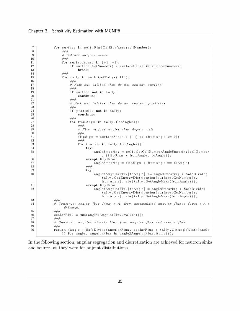
Chapter 3. Sensitivity Estimation with MCNP6
7 for s u r f a c e in s e l f . F indCe l lSur f a ce s ( cellNumber ) :8 ###9 # Extract sur face sense
10 ###11 for su r f a c eSen s e in (+1 , −1) :12 i f s u r f a c e . GetNumber ( ) ∗ su r f a c eSen s e in surfaceNumbers :13 break ;14 ###15 for t a l l y in s e l f . GetTal lys ( ’ f 1 ’ ) :16 ###17 # Kick out t a l l i e s t ha t do not contain sur face18 ###19 i f s u r f a c e not in t a l l y :20 continue ;21 ###22 # Kick out t a l l i e s t ha t do not contain p a r t i c l e s23 ###24 i f p a r t i c l e s not in t a l l y :25 continue ;26 ###27 for fromAngle in t a l l y . GetAngles ( ) :28 ###29 # Fl ip sur face ang l e s t ha t depart c e l l30 ###31 f l i p S i g n = sur f a c eSen s e ∗ (−1) ∗∗ ( fromAngle <= 0) ;32 ###33 for toAngle in t a l l y . GetAngles ( ) :34 try :35 angleSmearing = s e l f . GetCellNumberAngleSmearing ( cellNumber
, ( f l i p S i g n ∗ fromAngle , toAngle ) ) ;36 except KeyError :37 angleSmearing = f l i p S i g n ∗ fromAngle == toAngle ;38 ###39 try :40 angle2AngularFlux [ toAngle ] += angleSmearing ∗ SafeDiv ide (
t a l l y . GetEnergyDistr ibut ion ( s u r f a c e . GetNumber ( ) ,fromAngle ) , abs ( t a l l y . GetAngleMean ( fromAngle ) ) ) ;
41 except KeyError :42 angle2AngularFlux [ toAngle ] = angleSmearing ∗ SafeDiv ide (
t a l l y . GetEnergyDistr ibut ion ( s u r f a c e . GetNumber ( ) ,fromAngle ) , abs ( t a l l y . GetAngleMean ( fromAngle ) ) ) ;
43 ###44 # Construct s c a l a r f l u x (\ phi ∗ A) from accumulated angular f l u x e s (\ p s i ∗ A ∗
d\Omega)45 ###46 s ca l a rF lux = sum( angle2AngularFlux . va lue s ( ) ) ;47 ###48 # Construct angular d i s t r i b u t i o n from angular f l u x and s ca l a r f l u x49 ###50 return ang le : Sa feDiv ide ( angularFlux , s ca l a rF lux ∗ t a l l y . GetAngleWidth ( ang le
) ) for angle , angularFlux in angle2AngularFlux . i tems ( ) ;
In the following section, angular segregation and discretization are achieved for neutron sinksand sources as they were for adjoint distributions.
35

Chapter 3. Sensitivity Estimation with MCNP6
3.2.4 Angular segregation and discretization of neutron sinks andsources
Depending on the nature of the input parameter p, ∆A (or p∂A∂p
) can correspond to a neutron
sink mechanism, neutron source mechanism, or both–essentially the second and/or thirdterms in Equation 2.4. For neutron sinks, ∆Aψ is the distribution rate of neutrons precedinga reaction:
∆Asinkψ ≡ Σsink(~r, E) ψ(~r, E, ~Ω) = nsink(~r, E, ~Ω); (3.36)
for neutron sources, ∆Aψ is the distribution rate of neutrons following a reaction:
∆Asourceψ ≡∞∫
0
dE ′∫4π
d~Ω′ νsource(E′) Σsource(~r, E
′ → E, ~Ω′ → ~Ω) ψ(~r, E ′, ~Ω′)
= nsource(~r, E, ~Ω).
(3.37)
For both cases, the same procedure can be used on ∆Aψ to segregate angular dependencefrom the rest:
ψ†∆Aψ = φ†(~r, E)
∫~Ω
d~Ω α†(~r, E, ~Ω) nx(~r, E, ~Ω)
= φ†(~r, E)
∫~Ω
d~Ω nx(~r, E, ~Ω)∫~Ω
d~Ω nx(~r, E, ~Ω)
∫~Ω
d~Ω α†(~r, E, ~Ω) nx(~r, E, ~Ω)
= φ†(~r, E)nx(~r, E)
nx(~r, E)
∫~Ω
d~Ω α†(~r, E, ~Ω) nx(~r, E, ~Ω)
= φ†(~r, E) nx(~r, E)
∫~Ω
d~Ω α†(~r, E, ~Ω)nx(~r, E, ~Ω)
nx(~r, E),
(3.38)
where nx is either the neutron source or sink distribution.When the neutron sink distribution rate Equation 3.36 is examined, it is clear that
angular dependence rests entirely within ψ. Therefore, the fraction in Equation 3.38 isphysically equivalent to Equation 3.4 for neutron sinks. The neutron sink distribution rateoutside of the directional integral in Equation 3.38 is equal to the neutron sink reaction rate; the rate at which neutrons are lost is equal to the rate at which they incur sink reactions.Therefore, for neutron sinks, the fraction can be replaced with α and nsink(~r, E) can be
36

Chapter 3. Sensitivity Estimation with MCNP6
replaced with the linear functional reaction rate Rsink(~r, E):
ψ†∆Asinkψ = φ†(~r, E) Rsink(~r, E)
∫~Ω
d~Ω α†(~r, E, ~Ω) α(~r, E, ~Ω). (3.39)
When Equation 3.38 is considered for neutron sources, the realization is made that theneutron source distribution rate is related to the source reaction rate , but not in a straightfor-ward manner. With most fissions, thermal neutrons beget multiple fast neutrons, distributedin a fission energy spectrum. (n, 2n) and (n, 3n) always birth two or three neutrons respec-tively at lower kinetic energies. Scattering releases one neutron at a lower kinetic energy,except within thermal energies, where the neutron may be energized. FM4 cell flux mul-tiplier tallies identify the distribution rate of neutrons at the onset of reactions, but knownothing of the neutrons after the reaction occurs. Tally tagging, a new feature in MCNP6,is uniquely suited to provide post-reaction information.
Any particle is able to contribute to a tally for a neutron sink, but by restricting a tallyto only those particles that are born in a manner corresponding to p, a neutron source couldbe extracted. Tally tagging can be considered as a form of particle-wise filtering; it allowsfor binning of tallies according to how particles are tagged and a particle’s tag is determinedby how it is born (some combination of the cell, isotope, and reaction type) [Pelowitz et al.,2011]. All that remains is to form a tallying scheme that efficiently extracts neutron sourcerate distributions.
As depicted in Figure 3.4, all neutrons born within a cell have one of two ultimate fates:to collide within the birth cell (paths b and d), or to escape from that cell before colliding(paths a, c, and e). The rate of occurrence of the first fate can be extracted with an FM4 cell
2
1
a
c b
d
e
Figure 3.4: The five distinct paths for a particle born in a spherical shell until collision.
flux multiplier tally for collision reactions (MT = 1). The rate of the second can be countedby using F 1 surface current tallies to tabulate net surface crossings. The complication of
37

Chapter 3. Sensitivity Estimation with MCNP6
reentrant cells can be overcome with angular binning. For example, referring to Figure 3.4again, if surfaces 1 and 2 have inward/outward angular binning (with respect to the birthcell), paths are tallied as in Table 3.1. By subtracting inward surface crossing from outward
Surface # Sense Paths1 inward d+ e1 outward c+ d+ e2 inward . . .2 outward a+ e
Table 3.1: Particle path contributions to directional surface crossing tallies.
crossings, net leakages can be obtained:
F 11,out − F 1
1,in + F 12,out − F 1
2,in = (c+ d+ e)− (d+ e) + (a+ e)− () = (a+ c+ e). (3.40)
This expression can be generalized for a cell c bounded by any number of surfaces s, reentrantor not (even multiply so):
net leakage =∑s
∑µ
((−1)(∆µ is inward) F 1
s,µ
). (3.41)
Angular distributions are extracted in the usual manner but with tally tags. With schemesdefined for extracting neutron source rates and distributions, the segregated bilinear func-tional (Equation 3.38) can be written for neutron sources:
ψ†∆Asourceψ = φ†(~r, E) nsource(~r, E)
∫~Ω
d~Ω α†(~r, E, ~Ω) αsource(~r, E, ~Ω). (3.42)
The expressions for neutron sinks and sources (Equations 3.39 and 3.42) can now bediscretized, written entirely in terms of standard MCNP6 tallies. As before, cell fluxes andcell reaction rate densities can be replaced with F 4 cell flux tallies and FM4 cell flux multipliertallies, respectively:
ψ†∆Asinkψ ∼= F 4†c (E) FM4
c,z,x(E)∑i
∆µi α†c(E, µi) αc(E, µi), (3.43)
ψ†∆Asourceψ ∼= F 4†c (E) nc,source(E)
∑i
∆µi α†c(E, µi) αc,source(E, µi), (3.44)
where c is the cell index, i is the discrete angular bin index, nc,source(E) is the neutron source
38

Chapter 3. Sensitivity Estimation with MCNP6
rate, defined as:
nc,source(E) = FM4c,z=∗,x=1(E) +
∑s
∑µ
((−1)(∆µ is inward) F 1
s,µ
), (3.45)
with directional mapping taken into account, and all cell angular distributions αc are definedas in Equation 3.35. It won’t be shown until Section 3.5, but for now it is taken for grantedthat adjoint distributions can be extracted in the same manner as forward flux, within anadjoint transport calculation. Every bilinear functional product is performed externally toMCNP6 over discrete regions of phase space, in which physical quantities are averaged overcells, angles, and energy bins. While the treatment is not exact, the discrete summation overall phase space approaches the continuous integral as the bin size is shrunk to arbitrarilysmall size.
The neutron source surface accumulation scheme with tally tagging for both source rateand angular distribution is demonstrated in the GetCellSourceEnergyAngularDistributionmethod of the McnpOutputFile class within ParseMcnp.py:
Algorithm 3.4: GetCellSourceEnergyAngularDistribution1 def GetCel lSourceEnergyAngularDistr ibut ion ( s e l f , cellNumber , materialNumber , za ,
reactionNumber , p a r t i c l e s = ’np ’ ) :2 ###3 # Accumulate a l l p o s s i b l e source p a r t i c l e t r a c k s4 # Par t i c l e s can o r i g i n a t e from wi th in any s i s t e r l e a f c e l l5 ###6 su r f a c eCro s s i ngAngu l a rD i s t r i bu t i on = ;7 co l l i s ionReact ionNumber = 1 ;8 c o l l i s i o n s = 0 . ;9 ###
10 for r o o t C e l l in s e l f . FindRootCel ls ( cellNumber ) :11 ###12 # Extract root c e l l su r face numbers f o r sense13 ###14 rootCel lSurfaceNumbers = r o o t C e l l . GetSurfaceNumbers ( ) ;15 for s i s t e r C e l l in s e l f . F indLea fCe l l s ( r o o t C e l l ) :16 ###17 # Build t a l l y tag18 ###19 ta l lyTag = (1 e5 ∗ s i s t e r C e l l . GetNumber ( ) ) + za + (1 e−5 ∗
reactionNumber ) ;20 ###21 # Accumulate root c e l l bounding sur face c ro s s i n g s22 # Root c e l l bounding sur face c ro s s i n g s record p a r t i c l e s t ha t c o l l i d e
ou t s i d e o f the root c e l l23 ###24 for s u r f a c e in s e l f . F indCe l lSur f a ce s ( r o o t C e l l . GetNumber ( ) ) :25 ###26 # Kick out transformed sur f a c e s27 # This may be dangerous , but was the b e s t conceived way to
e l im ina t e the l a s e r por t su r f a c e s28 ###29 i f s u r f a c e . GetTransformationNumber ( ) :30 continue ;31 ###
39

Chapter 3. Sensitivity Estimation with MCNP6
32 # Extract sur face sense33 ###34 for su r f a c eSen s e in (+1 , −1) :35 i f s u r f a c e . GetNumber ( ) ∗ su r f a c eSen s e in
rootCel lSurfaceNumbers :36 break ;37 ###38 # I t e r a t e over F1 t a l l i e s39 ###40 for t a l l y in s e l f . GetTal lys ( ’ f 1 ’ ) :41 ###42 # Kick out t a l l i e s t ha t do not contain sur face43 ###44 i f s u r f a c e not in t a l l y :45 continue ;46 ###47 # Kick out t a l l i e s t ha t do not contain p a r t i c l e s48 ###49 i f p a r t i c l e s not in t a l l y :50 continue ;51 ###52 # Kick out t a l l i e s t ha t do not contain t a l l y tag53 ###54 i f ta l lyTag not in t a l l y :55 continue ;56 ###57 # Preserve sur face c ro s s ing t a l l y f o r l a t e r58 ###59 s u r f a c e C r o s s i n g T a l l y = t a l l y ;60 for fromAngle in t a l l y . GetAngles ( ) :61 ###62 # Fl ip sur face ang l e s t ha t depart c e l l63 ###64 f l i p S i g n = sur f a c eSen s e ∗ (−1) ∗∗ ( fromAngle <= 0) ;65 ###66 for toAngle in t a l l y . GetAngles ( ) :67 try :68 angleSmearing = s e l f . GetCellNumberAngleSmearing (
cellNumber , ( f l i p S i g n ∗ fromAngle , toAngle ) ) ;69 except :70 angleSmearing = f l i p S i g n ∗ fromAngle == toAngle ;71 ###72 try :73 su r f a c eCro s s i ngAngu la rD i s t r i bu t i on [ toAngle ] += −
f l i p S i g n ∗ angleSmearing ∗ t a l l y .GetEnergyDistr ibut ion ( s u r f a c e . GetNumber ( ) ,ta l lyTag , fromAngle ) ;
74 except KeyError :75 su r f a c eCro s s i ngAngu la rD i s t r i bu t i on [ toAngle ] = −
f l i p S i g n ∗ angleSmearing ∗ t a l l y .GetEnergyDistr ibut ion ( s u r f a c e . GetNumber ( ) ,ta l lyTag , fromAngle ) ;
76 ###77 # Accumulate c o l l i s i o n s wi th in s i s t e r l e a f c e l l s78 # S i s t e r l e a f c e l l c o l l i s i o n s record p a r t i c l e s t ha t c o l l i d e wi th in the
root c e l l79 ###80 s i s t e rCe l lMater ia lNumber = s i s t e r C e l l . GetMaterialNumber ( ) ;81 ###82 # Divide by number o f p hy s i c a l i n s t a n t i a t i o n s o f s i s t e r c e l l
40

Chapter 3. Sensitivity Estimation with MCNP6
83 ###84 d i v i s o r = 1 . ;85 i f s e l f . GetIsMult ip lyRootedLeafCe l l ( s i s t e r C e l l . GetNumber ( ) ) :86 d i v i s o r ∗= len ( s e l f . GetMult ip lyRootedLeafCel l ( s i s t e r C e l l . GetNumber
( ) ) ) ;87 ###88 # I t e r a t e over FM4 t a l l i e s89 ###90 for t a l l y in s e l f . GetTal lys ( ’ fm4 ’ ) :91 ###92 # Kick out t a l l i e s t ha t do not contain s i s t e r c e l l93 ###94 i f s i s t e r C e l l not in t a l l y :95 continue ;96 ###97 # Kick out t a l l i e s t ha t do not contain p a r t i c l e s98 ###99 i f p a r t i c l e s not in t a l l y :
100 continue ;101 ###102 # Kick out t a l l i e s t ha t do not contain t a l l y tag103 ###104 i f ta l lyTag not in t a l l y :105 continue ;106 ###107 for m u l t i p l i e r B i n in t a l l y . GetMul t ip l i e rB ins ( ) :108 ###109 # Divide out non−uni ty mu l t i p l i e r s110 ###111 m u l t i p l i e r = SafeDiv ide ( s i s t e r C e l l . GetVolume ( ) , abs (
m u l t i p l i e r B i n [ 1 ] ) ) ;112 ###113 c o l l i s i o n s += SafeDiv ide ( t a l l y . GetEnergyDistr ibut ion (
s i s t e r C e l l . GetNumber ( ) , ta l lyTag , (s i s te rCe l lMater ia lNumber , co l l i s ionReact ionNumber ) ) ∗m u l t i p l i e r , d i v i s o r ) ;
114 ###115 # Construct source neutron ra te116 ###117 sourceRate = sum( su r f a c eCro s s i ngAngu la rD i s t r i bu t i on . va lue s ( ) ) + c o l l i s i o n s ;118 ###119 # Construct source neutron angular d i s t r i b u t i o n120 ###121 angle2AngularFlux = ang le : Sa feDiv ide ( su r f a c eCro s s ing s , abs (
s u r f a c e C r o s s i n g T a l l y . GetAngleMean ( ang le ) ) ) for angle , s u r f a c e C r o s s i n g s insu r f a c eCro s s i ngAngu la rD i s t r i bu t i on . i tems ( ) ;
122 s ca l a rF lux = sum( angle2AngularFlux . va lue s ( ) ) ;123 a n g u l a r D i s t r i b u t i o n = ang le : Sa feDiv ide ( angularFlux , s ca l a rF lux ∗
s u r f a c e C r o s s i n g T a l l y . GetAngleWidth ( ang le ) ) for angle , angularFlux inangle2AngularFlux . i tems ( ) ;
124 ###125 return sourceRate , a n g u l a r D i s t r i b u t i o n ;
Bilinear functionals are constructed and then normalized within the CalculateResponse-ImplicitSensitivitys method of the SensitivityUncertaintyCalculator class in Parse-
Mcnp.py in a manner similar to Algorithm 3.1:
Algorithm 3.5: CalculateResponseImplicitSensitivitys
41

Chapter 3. Sensitivity Estimation with MCNP6
1 def C a l c u l a t e R e s p o n s e I m p l i c i t S e n s i t i v i t y s ( s e l f , response , sumOverCells , sumOverZas, sumOverReactions ) :
2 forwardMcnp = s e l f . GetForwardMcnp ( ) ;3 ###4 # Extract response por t i ons5 ###6 div idend = response . GetDividend ( ) ;7 d i v i s o r = response . GetDivisor ( ) ;8 ###9 # Extract t o t a l response
10 ###11 tota lResponse = forwardMcnp . GetTotal ( d iv idend ) ;12 s i g n s = [ + 1 ] ;13 i f d i v i s o r :14 tota lResponse ∗= SafeDiv ide (1 , forwardMcnp . GetTotal ( d i v i s o r ) ) ;15 s i g n s . append(−1) ;16 ###17 # Kick out responses f o r which e i t h e r the d iv idend or d i v i s o r are zero−va lued18 ###19 i f not tota lResponse :20 return ;21 ###22 # Perturba t ion23 ###24 per turbat i on = response . GetPerturbat ion ( ) ;25 i s P e r t u r b a t i o n = bool ( pe r turbat i on ) ;26 i f i s P e r t u r b a t i o n :27 perturbCellNumber , perturbZa , perturbReactionNumber = per turbat i on [ 0 ] ;28 ###29 # c e l l number −−> importance30 # Non−dimensional importance i s equa l to the ad j o in t f l u x mu l t i p l i e d by the
volume , or the ad j o in t p a r t i c l e track−l e n g t h31 # c e l l number −−> ad j o in t angular d i s t r i b u t i o n32 ###33 cel lNumber2Importance = ;34 cel lNumber2AdjointAngular = ;35 for s i gn in s i g n s :36 adjointMcnp = ReadMcnpFile ( ’ . o ’ . format ( re sponse . GetFileName ( ’−adj ’ .
format ( forwardMcnp . GetFileName ( ) . r e p l a c e ( ’ . o ’ , ’ ’ ) ) , s i gn ) ) ) ;37 for cellNumber in adjointMcnp . GetTa l ly Ind i ce s ( ’ f 4 ’ ) :38 try :39 cel lNumber2Importance [ cellNumber ] += s ign ∗ adjointMcnp .
GetCel l ImportancePerResponseEnergyDistr ibut ion ( cellNumber ) ;40 cel lNumber2AdjointAngular [ cel lNumber ] = adjointMcnp .
GetCe l lAngu la rDi s t r ibut ionEnergyDi s t r ibut ion ( cellNumber ) ;41 except KeyError :42 cel lNumber2Importance [ cellNumber ] = s i gn ∗ adjointMcnp .
GetCel l ImportancePerResponseEnergyDistr ibut ion ( cellNumber ) ;43 cel lNumber2AdjointAngular [ cel lNumber ] = adjointMcnp .
GetCe l lAngu la rDi s t r ibut ionEnergyDi s t r ibut ion ( cellNumber ) ;44 ###45 # I t e r a t e over reac t i on ra te t a l l y s46 ###47 k e y 2 I m p l i c i t S e n s i t i v i t y = ;48 for cellNumber , m u l t i p l i e r B i n s in so r t ed ( forwardMcnp . GetTa l ly Ind i ce s ( ’ fm4 ’ ) .
i tems ( ) ) :49 ###50 # Kick out non−rooted c e l l s51 # Only root c e l l s have meaningful angular d i s t r i b u t i o n s52 ###
42

Chapter 3. Sensitivity Estimation with MCNP6
53 i f forwardMcnp . FindCel l ( cellNumber ) . GetUniverse ( ) :54 continue ;55 ###56 # Ce l l importance energy d i s t r i b u t i o n57 ###58 importance = cellNumber2Importance [ cellNumber ] ;59 ###60 # Forward neutron s ink angular d i s t r i b u t i o n61 ###62 s inkAngular = forwardMcnp . GetCe l lAngu la rDi s t r ibut ionEnergyDi s t r ibut ion (
cellNumber ) ;63 ###64 # Sink angular i n t e g r a l65 ###66 s inkAngu la r In t eg ra l = s e l f . Ca l cu l a t eAngu la r In t eg ra l (
cel lNumber2AdjointAngular [ cel lNumber ] , s inkAngular ) ;67 ###68 # I t e r a t e over mu l t i p l i e r b ins69 ###70 for materialNumber , reactionNumber in m u l t i p l i e r B i n s :71 try :72 ###73 # Extract s i n g l e−za from mater ia l number74 ###75 za = forwardMcnp . GetMaterialNumber2SingleZa ( ) [ materialNumber ] ;76 except KeyError :77 ###78 # Kick out non−s i n g l e−za mater ia l numbers79 ###80 continue ;81 ###82 # Kick out i f i nd i c e s don ’ t match pe r tu rba t i on ind i c e s83 ###84 i f i s P e r t u r b a t i o n :85 # c86 i f perturbCellNumber not in (None , cellNumber ) :87 continue ;88 # z89 i f perturbZa not in (None , za ) :90 continue ;91 # x92 i f perturbReactionNumber not in (None , reactionNumber ) :93 continue ;94 ###95 # Neutron s ink96 ###97 sinkRate = forwardMcnp . GetCe l lS inkEnergyDis t r ibut ion ( cellNumber ,
materialNumber , reactionNumber ) ;98 ###99 # Kick out zero−va lued neutron s ink s
100 # I f the neutron s ink i s zero , the neutron source c e r t a i n l y i s , too101 ###102 i f not f l o a t ( s inkRate ) :103 continue ;104 ###105 # Neutron source106 ###107 sourceRate , sourceAngular = 0 . , 0 . ;108 i f reactionNumber in impl ic i tReact ionNumbers and
impl ic i tReact ionNumbers [ reactionNumber ] :
43

Chapter 3. Sensitivity Estimation with MCNP6
109 sourceRate , sourceAngular = forwardMcnp .GetCel lSourceEnergyAngularDistr ibut ion ( cellNumber ,materialNumber , za , reactionNumber ) ;
110 ###111 # Source angular i n t e g r a l112 ###113 sourceAngu la r In t eg ra l = s e l f . Ca l cu l a t eAngu la r In t eg ra l (
cel lNumber2AdjointAngular [ cel lNumber ] , sourceAngular ) ;114 ###115 # Calcu la t e imp l i c i t s e n s i t i v i t y116 # The imp l i c i t s e n s i t i v i t y due to source neutrons be longs to the
energy b ins t ha t caused them ##### For MT=4, 16 , 17 t h i s i s f i n e. . . f o r MT=18, we need to weight by nu(E ’) .
117 ###118 i m p l i c i t S e n s i t i v i t y = importance ∗ s inkRate ∗ s i nkAngu la r In t eg ra l ;119 i m p l i c i t S e n s i t i v i t y += SafeDiv ide ( s inkRate ∗ f l o a t ( importance ∗
sourceRate ∗ sourc eAngu la r In t eg ra l ) , f l o a t ( s inkRate ) ) ;120 ###121 # Kick out zero−va lued imp l i c i t s e n s i t i v i t y s122 ###123 i f not f l o a t ( i m p l i c i t S e n s i t i v i t y ) :124 continue ;125 ###126 # Square away summation ind i c e s127 ###128 key = [ ] ;129 ###130 i f not sumOverCells :131 key . append ( cellNumber ) ;132 ###133 i f not sumOverZas :134 key . append ( za ) ;135 ###136 i f not sumOverReactions :137 key . append ( reactionNumber ) ;138 ###139 key = tup l e ( key ) ;140 ###141 try :142 k e y 2 I m p l i c i t S e n s i t i v i t y [ key ] += i m p l i c i t S e n s i t i v i t y ;143 except KeyError :144 k e y 2 I m p l i c i t S e n s i t i v i t y [ key ] = i m p l i c i t S e n s i t i v i t y ;145 ###146 # Check imp l i c i t s e n s i t i v i t y d i s c r epanc i e s147 ###148 d i sc repancy = sum( ed . GetTotalElement ( ) for ed in k e y 2 I m p l i c i t S e n s i t i v i t y .
va lue s ( ) i f ed )149 i f abs ( d i s c repancy ) > 1e−3:150 Warning ( ’ :+.2% o f i m p l i c i t s e n s i t i v i t y i s unaccounted f o r in re sponse
‘\ ’ with s i n g l e−i s o t o p e r e a c t i o n r a t e s : ! ’ . format ( d iscrepancy ,response , ’ , ’ . j o i n ( s t r ( key ) for key in so r t ed ( k e y 2 I m p l i c i t S e n s i t i v i t y) ) ) ) ;
151 ###152 return k e y 2 I m p l i c i t S e n s i t i v i t y ;
44

Chapter 3. Sensitivity Estimation with MCNP6
3.3 Editing MCNP6 for elastic scatter tally tagging
At the time of this writing, the latest available version of MCNP6 is Beta 12 and its mostrelevant documentation is the MCNPX 2.7.E release memorandum [Pelowitz et al., 2011].Among the special designations for tally tags described in the document is an ‘elastic-scattered particle tag’ 0, designated for particles that have participated in an elastic scatter.Upon inspection of the moniker ‘0’, it is clear that it contains zero entropy bits; it cannotcontain enough information to identify a specific cell number, element, or isotope in whichthe elastic scatter occurs. Other than with this special designator, there is no way to filterparticles that have elastically scattered.
A patch composed of seven edits to five files (artf20729) was made to MCNP6, enablingthe new feature of the FTn TAG 4. Within colidn.F90 special treatment was written forelastic scatters when TAG=4. Within itally.F90 the input error checking was modified toallow for FTn TAG values up to four. Within annihilation gammas.F90, brems.F90, andttbr.F90, conditions specific to bremsstrahlung and annihilation photons for TAG=2,3 wereremoved.
Using this new tag type, particles undergoing elastic scatter in cell number CCCCC withisotope ZZAAA are assigned the production tag CCCCCZZAAA.00002, instead of 0. Conse-quently, elastic scatters are able to join inelastic scatters, (n, 2n), (n, 3n), and fissions aspossible birth reactions that can be tally tagged.
3.4 Constructing the adjoint source
In order to perform an adjoint transport calculation, the adjoint source must be constructedwith the proper distribution, units, and normalization. The adjoint source is defined inEquation 2.37 as:
S† ≡ ∂R
∂ψ. (3.46)
If working with φ rather than ψ is desired (scalar flux rather than angular flux), one can usethe chain rule:
∂R
∂ψ=∂R
∂φ
∂φ
∂ψ, (3.47)
and represent the last partial derivative as a Gateaux derivative:
∂φ
∂ψ=
ddtφ(ψ + tδψ)|t=0
δψ=
∂φ(ψ)∂ψ
δψ
δψ. (3.48)
45

Chapter 3. Sensitivity Estimation with MCNP6
From 3.13 it is clear that φ is linear in ψ, so:
∂φ
∂ψ=φ(δψ)
δψ. (3.49)
Since δψ can move through the directional integral:
∂φ
∂ψ= 4π. (3.50)
In a subtle way, this means that the adjoint source is isotropic; the presence of neutrons isall that matters for responses, not the direction of travel. If one wishes to convert betweenan angular adjoint source S†(~r, E, ~Ω) and a scalar adjoint source S†(~r, E), a factor of 4π isall that is needed.
For linear functional responses with the form of Equation 2.16, the angular adjoint sourceof Equation 2.48 can be converted to a scalar adjoint source, distributed over (~r, E) in neutronphase space:
S† =
(4π
R
〈Hψ〉
)H =
(4πR
〈Hψ〉
)Hφφ. (3.51)
Equivalently, for ratios of linear functional responses with the form of Equation 2.21, the an-gular adjoint source of Equation 2.50 can be converted to a scalar adjoint source, distributedover (~r, E) in neutron phase space:
S† =
(4π
R
〈H1ψ〉
)H1 −
(4π
R
〈H2ψ〉
)H2 =
(4πR
〈H1ψ〉
)H1φ
φ−(
4πR
〈H2ψ〉
)H2φ
φ. (3.52)
Upon inspection of these equations, it is evident that contributions from response divi-dends are positive and those from response divisors (if they exist) are negative. This presentsthe likely possibility of locally and/or globally negative adjoint sources. Negative sourceweights cannot be used in a calculation. However, the importance scales linearly with theadjoint source; the importance can be extracted from a single calculation or summed over anynumber of independent adjoint calculations given portions of the adjoint source. Knowingthis, one calculation is automatically performed for just the dividend and one is performedfor just the divisor, if it exists. The results are then superimposed, giving the dividendimportance positive sign and the divisor negative sign.
To summarize, the algorithm for extracting adjoint sources for a given response takesits dividend and divisor (if it exists) and iterates over all FM4 cell flux multiplier tallieswithin a forward MCNP6 calculation, finding those that match with the constituents ofthe response and adjusting for the required multiplicity and sign. These linear functionalsare accumulated over all isotopes, but binned over cell and energy. The results are thenmultiplied by 4π times the total response and divided by the total of that linear functional
46

Chapter 3. Sensitivity Estimation with MCNP6
times each cell’s scalar flux. The GetCellAdjointSourceEnergyDistribution method ofthe McnpOutputFile class in ParseMcnp.py is responsible for these steps and its source codeis included below to allay any confusion:
Algorithm 3.6: GetCellAdjointSourceEnergyDistribution1 def GetCe l lAdjo intSourceEnergyDis t r ibut ion ( s e l f ,
cellNumberMaterialNumberReactionNumbers ) :2 ###3 a s s e r t ( s e l f . GetIsForward ( ) ) ;4 ###5 # Check t ha t a l l q uan t i t y s e x i s t w i th in the same c e l l6 ###7 a s s e r t (1 == len ( item [ 0 ] for item in cellNumberMaterialNumberReactionNumbers )
) ;8 ###9 # Sum of c e l l r eac t i on ra t e s
10 ###11 react ionRate = sum( s e l f . GetCel lReact ionRateEnergyDist r ibut ion ( cellNumber ,
materialNumber , reactionNumber ) for cellNumber , materialNumber ,reactionNumber in cellNumberMaterialNumberReactionNumbers ) ;
12 react ionRate ∗= 4 ∗ pi ;13 ###14 # Ce l l t rack l eng t h and volume15 ###16 cellNumber = cellNumberMaterialNumberReactionNumbers [ 0 ] [ 0 ] ;17 trackLength , volume = s e l f . GetCel lTrackLengthVolumeEnergyDistr ibution (
cellNumber ) ;18 ###19 totalTrackLength = 0 . ;20 i f i s i n s t a n c e ( trackLength , EnergyDis t r ibut ion ) :21 totalTrackLength = trackLength . GetTotalElement ( ) ;22 ###23 tota lReact ionRate = ad jo in tSource = 0 . ;24 i f i s i n s t a n c e ( react ionRate , EnergyDis t r ibut ion ) :25 tota lReact ionRate = react ionRate . GetTotalElement ( ) ;26 ad jo in tSource = SafeDiv ide ( react ionRate ∗ volume , trackLength ) ;27 ###28 # In t e r p o l a t e non−zero va lue s below 2e−829 ###30 ad jo in tSource . ZeroTerp ( ) ;31 ###32 return ( tota lReact ionRate , totalTrackLength , volume , ad jo in tSource ) ;
Within the WriteAdjointInput method of the McnpOutputFile class in ParseMcnp.py,the weights and distributions of adjoint sources are calculated and formatted for adjointinput files. In some instances, the adjoint source must be summed over regions of neutronphase space: leaf cells are summed for their contributions to root cells (cell universes areorganized in tree data structures [Weisstein, 2011d]), and energy distributions are summedover energy bins. In both cases, the procedure is to divide the total response by the totalneutron track length and multiplying by the total volume, or equivalently, to divide the total
47

Chapter 3. Sensitivity Estimation with MCNP6
response by the average neutron flux:
S† =
∑c
∑g Rc(Eg)∑
c Vc∑
g φc(Eg)
∑c
Vc, (3.53)
where c and g are the cell and energy bin indices, respectively. Further inquiry is directedto the method’s source below:
Algorithm 3.7: WriteAdjointInput1 def WriteAdjointInput ( s e l f ) :2 def Cel lPath2Str ing ( c e l lPa th ) :3 pathStr ing = ’ ’ ;4 i f l en ( c e l lPa th ) > 1 :5 pathStr ing = ’ ( ) ’ ;6 ###7 return pathStr ing . format ( ’ < ’ . j o i n ( ’ ’ . j o i n ( s t r ( cellNumber ) for
cellNumber in cel lNumbers ) for cel lNumbers in c e l lPa th ) ) ;8 ###9 def CellPath2PathLengthRange ( c e l lPa th ) :
10 numberOfPaths = 1 ;11 for c e l l s in c e l lPa th :12 numberOfPaths ∗= len ( c e l l s ) ;13 return range ( numberOfPaths ) ;14 ###15 # Reset automatic input16 ###17 s e l f . ResetAutoInput ( ) ;18 ###19 # Append automatic input f i l ename20 ###21 s e l f . AppendAutoInputFileName ( ’ adj ’ ) ;22 ###23 # c e l l number −−> r a d i i24 ###25 rootCel lNumber2Radii = ;26 for r o o t C e l l in s e l f . GetCel l s ( ) :27 ###28 # Kick out non−rooted c e l l s29 # The PDS ( po s i t i on d i r e c t i on sampling ) coord inate systems are de f ined
only f o r root c e l l s and t h e i r r a d i i30 ###31 i f r o o t C e l l . GetUniverse ( ) :32 continue ;33 ###34 r a d i i = so r t ed ( s u r f a c e . GetDimension ( ) for s u r f a c e in s e l f . F indCe l lSur f a ce s
( r o o t C e l l . GetNumber ( ) ) i f s u r f a c e . GetIsSphere ( ) ) ;35 i f 1 == len ( r a d i i ) :36 r a d i i . append ( 0 . ) ;37 r a d i i . r e v e r s e ( ) ;38 ###39 rootCellNumber2Radii [ r o o t C e l l . GetNumber ( ) ] = r a d i i ;40 ###41 mnemonic2NewLines = ;42 ###43 # Necessary ad j o in t t a l l y s44 ###45 nece s sa ry = s e l f . F indNecessaryTal lys ( doAdjoint = True ) ;
48

Chapter 3. Sensitivity Estimation with MCNP6
46 ###47 # F1 and F4 t a l l y l i n e s48 ###49 tallyNumber = 0 ;50 for mnemonic in ( ’ f 1 ’ , ’ f 4 ’ ) :51 mnemonic2NewLines [ mnemonic ] = [ WordArrange ( words = sor t ed ( nece s sa ry [
mnemonic ] ) , p r e f i x = ’ f : n ’ . format (10 ∗ tallyNumber + i n t ( f l o a t (mnemonic [−1]) ) ) ) ] ;
52 ###53 # Build miss ing ang le b in l i n e s54 ###55 numberOfAngleBins = s e n s e F i l e . GetParameter ( ’ numberOfAngleBins ’ ) ;56 ang leBins = Array ( l i s t (−1. + 2 . ∗ ( index + 1) / numberOfAngleBins for index in
range ( i n t ( numberOfAngleBins ) ) ) )57 mnemonic2NewLines [ ’ ang leBins ’ ] = [ WordArrange ( words = angleBins , format = ’
:+.2 f ’ , p r e f i x = ’ c0 ’ ) ] ;58 ###59 # Build miss ing energy bin l i n e s60 ###61 energyBinsPerDecade = s e n s e F i l e . GetParameter ( ’ energyBinsPerDecade ’ ) ;62 energyBins = LogFloats ( perDecade = i n t ( energyBinsPerDecade ) ) ;63 mnemonic2NewLines [ ’ energyBins ’ ] = [ WordArrange ( words = energyBins , format = ’
: . 4E ’ , p r e f i x = ’ e0 ’ ) ] ;64 ###65 # Add/ rep l ace nps card66 ###67 nps = 1e8 ;68 npsCard = ’ nps :G ’ . format ( nps ) ;69 s e l f . ReplaceAddAutoInputCard ( ’ nps ’ , npsCard ) ;70 ###71 # Dele te kcode and ksrc cards72 ###73 s e l f . DeleteAutoInputCard ( ’ kcode ’ ) ;74 s e l f . DeleteAutoInputCard ( ’ k s r c ’ ) ;75 ###76 # Add/ rep l ace mode card77 ###78 modeCard = ’mode n ’ ;79 s e l f . ReplaceAddAutoInputCard ( ’mode ’ , modeCard ) ;80 ###81 # Add/ rep l ace mgopt card82 ###83 mgoptCard = ’ mgopt a :G $ ’ . format ( s e n s e F i l e . GetParameter ( ’
numberOfEnergyBins ’ ) − 1 , modeCard ) ;84 s e l f . ReplaceAddAutoInputCard ( ’ mgopt ’ , mgoptCard ) ;85 ###86 # Convert l i b r a r y s u f f i x e s87 ###88 mult iGroupSuf f ix = ’ . : 3 ’ . format ( L i b r a r y S u f f i x ( i sPointWise = False ,
temperature = s e n s e F i l e . GetParameter ( ’ systemTemperature ’ ) ) ) ;89 s e l f . GetMcnpInputFile ( ) . autoInputRaw = ReCompile ( r ’ \ .\d\dc ’ , 2 | 8) . sub (
mult iGroupSuff ix , s e l f . GetAutoInputRaw ( ) ) ;90 ###91 # Add/ rep l ace cut card92 ###93 cutCard = ’ cut : n j 20 .0 ’ ;94 s e l f . ReplaceAddAutoInputCard ( ’ cut ’ , cutCard ) ;95 ###96 # Dele te a l l forward t a l l i e s97 # Dele te t a l l y comment cards , thermal s c a t t e r i n g l i b r a r i e s , and t a l l y t ag s
49
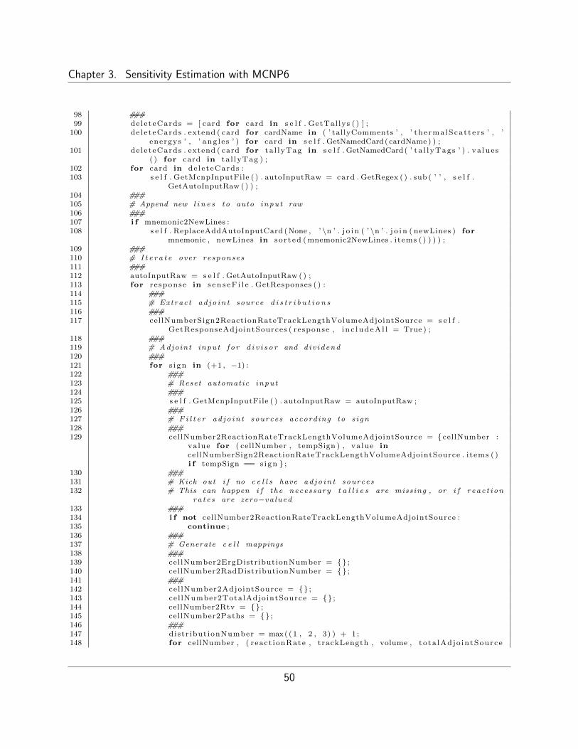
Chapter 3. Sensitivity Estimation with MCNP6
98 ###99 de le teCards = [ card for card in s e l f . GetTal lys ( ) ] ;
100 de le teCards . extend ( card for cardName in ( ’ tallyComments ’ , ’ the rma lSca t t e r s ’ , ’energys ’ , ’ ang l e s ’ ) for card in s e l f . GetNamedCard( cardName ) ) ;
101 de le teCards . extend ( card for ta l lyTag in s e l f . GetNamedCard( ’ ta l l yTags ’ ) . va lue s( ) for card in ta l lyTag ) ;
102 for card in de le teCards :103 s e l f . GetMcnpInputFile ( ) . autoInputRaw = card . GetRegex ( ) . sub ( ’ ’ , s e l f .
GetAutoInputRaw ( ) ) ;104 ###105 # Append new l i n e s to auto input raw106 ###107 i f mnemonic2NewLines :108 s e l f . ReplaceAddAutoInputCard (None , ’ \n ’ . j o i n ( ’ \n ’ . j o i n ( newLines ) for
mnemonic , newLines in so r t ed ( mnemonic2NewLines . i tems ( ) ) ) ) ;109 ###110 # I t e r a t e over responses111 ###112 autoInputRaw = s e l f . GetAutoInputRaw ( ) ;113 for re sponse in s e n s e F i l e . GetResponses ( ) :114 ###115 # Extract ad j o in t source d i s t r i b u t i o n s116 ###117 cel lNumberSign2ReactionRateTrackLengthVolumeAdjointSource = s e l f .
GetResponseAdjointSources ( response , i n c l u d e A l l = True ) ;118 ###119 # Adjoint input f o r d i v i s o r and d iv idend120 ###121 for s i gn in (+1 , −1) :122 ###123 # Reset automatic input124 ###125 s e l f . GetMcnpInputFile ( ) . autoInputRaw = autoInputRaw ;126 ###127 # F i l t e r ad j o in t sources according to s i gn128 ###129 cellNumber2ReactionRateTrackLengthVolumeAdjointSource = cellNumber :
va lue for ( cellNumber , tempSign ) , va lue incel lNumberSign2ReactionRateTrackLengthVolumeAdjointSource . i tems ( )i f tempSign == s ign ;
130 ###131 # Kick out i f no c e l l s have ad j o in t sources132 # This can happen i f the necessary t a l l i e s are missing , or i f r eac t i on
ra t e s are zero−va lued133 ###134 i f not cel lNumber2ReactionRateTrackLengthVolumeAdjointSource :135 continue ;136 ###137 # Generate c e l l mappings138 ###139 cel lNumber2ErgDistributionNumber = ;140 cellNumber2RadDistributionNumber = ;141 ###142 cel lNumber2AdjointSource = ;143 ce l lNumber2TotalAdjointSource = ;144 cellNumber2Rtv = ;145 cellNumber2Paths = ;146 ###147 distr ibut ionNumber = max( ( 1 , 2 , 3) ) + 1 ;148 for cellNumber , ( react ionRate , trackLength , volume , to ta lAdjo intSource
50

Chapter 3. Sensitivity Estimation with MCNP6
, ad jo in tSource ) in so r t ed (cel lNumber2ReactionRateTrackLengthVolumeAdjointSource . i tems ( ) ) :
149 ###150 # Each l e a f c e l l has i t s own energy d i s t r i b u t i o n151 ###152 i f cellNumber not in cel lNumber2ErgDistributionNumber :153 cel lNumber2ErgDistributionNumber [ cellNumber ] =
distr ibut ionNumber ;154 ###155 # Increment to unique number156 ###157 distr ibut ionNumber += 1 ;158 ###159 # Each root c e l l has i t s own r a d i i160 ###161 for r o o t C e l l in s e l f . FindRootCel ls ( cellNumber ) :162 i f r o o t C e l l . GetNumber ( ) not in
cellNumber2RadDistributionNumber :163 cellNumber2RadDistributionNumber [ r o o t C e l l . GetNumber ( ) ] =
distr ibut ionNumber ;164 ###165 # Increment to unique number166 ###167 distr ibut ionNumber += 1 ;168 ###169 # c e l l number −−> ad j o in t source energy d i s t r i b u t i o n170 ###171 cel lNumber2AdjointSource [ cellNumber ] = ad jo in tSource172 ###173 # c e l l number −−> t o t a l ad j o in t source174 ###175 ce l lNumber2TotalAdjointSource [ cellNumber ] = to ta lAd jo in tSource ;176 ###177 # c e l l number −−> ( r eac t i on rate , t rack l eng th , volume )178 ###179 cellNumber2Rtv [ cellNumber ] = ( react ionRate , trackLength , volume )180 ###181 # c e l l number −−> c e l l paths182 ###183 cellNumber2Paths [ cellNumber ] = s e l f . GetCellNumberPaths ( cellNumber )
;184 ###185 # System ad jo in t source186 ###187 systemReactionRate = 0 . ;188 systemTrackLength = 0 . ;189 systemVolume = 0 . ;190 for react ionRate , trackLength , volume in cellNumber2Rtv . va lue s ( ) :191 systemReactionRate += react ionRate ;192 systemTrackLength += trackLength ;193 systemVolume += volume ;194 ###195 cellNumberPaths = sor t ed ( ( cellNumber , c e l l P a t h s ) for cellNumber ,
c e l l P a t h s in so r t ed ( cellNumber2Paths . i tems ( ) ) ) ;196 ###197 # sde f card198 ###199 sdefCard = ’ ’ ;200 ###201 # sde f l i n e
51

Chapter 3. Sensitivity Estimation with MCNP6
202 ###203 sdefCard += ’ s d e f c e l d rad f c e l d erg f c e l d wgt :G ’ . format
(1 , 2 , 3 , 1 . ) ;204 ###205 # ce l path ’ s206 ###207 sdefCard += WordArrange ( words = ( Ce l lPath2Str ing ( c e l lPa th ) for
cellNumber , c e l l P a t h s in cellNumberPaths for c e l lPa th in c e l l P a t h s) , p r e f i x = ’ \ n s i l ’ . format (1 ) ) ;
208 ###209 # l e a f c e l l wgt ’ s210 ###211 sdefCard += WordArrange ( words = ( ce l lNumber2TotalAdjointSource [
cellNumber ] for cellNumber , c e l l P a t h s in cellNumberPaths forc e l lPa th in c e l l P a t h s for pathNumber in CellPath2PathLengthRange (c e l lPa th ) ) , format = ’ :G ’ , p r e f i x = ’ \nsp d ’ . format (1 ) ) ;
212 ###213 # l e a f c e l l root c e l l rad d i s t r i b u t i o n ind i c e s214 ###215 sdefCard += WordArrange ( words = ( cellNumber2RadDistributionNumber [
rootCellNumber ] for cellNumber , c e l l P a t h s in cellNumberPaths forc e l lPa th in c e l l P a t h s for pathNumber in CellPath2PathLengthRange (c e l lPa th ) for rootCellNumber in ( abs ( c e l lPa th [−1] [−1]) , ) ) , p r e f i x= ’ \nds s ’ . format (2 ) ) ;
216 ###217 # l e a f c e l l root c e l l rad d i s t r i b u t i o n s218 ###219 rootCellNumbers = sor t ed ( rootCellNumber for cellNumber , c e l l P a t h s in
cellNumberPaths for c e l lPa th in c e l l P a t h s for rootCellNumber in (abs ( c e l lPa th [−1] [−1]) , ) ) ;
220 for rootCellNumber in rootCellNumbers :221 sdefCard += WordArrange ( words = rootCel lNumber2Radii [
rootCellNumber ] , format = ’ :G ’ , p r e f i x = ’ \ n s i ’ . format (cellNumber2RadDistributionNumber [ rootCellNumber ] ) ) ;
222 ###223 # l e a f c e l l erg d i s t r i b u t i o n ind i c e s224 ###225 sdefCard += WordArrange ( words = ( cel lNumber2ErgDistributionNumber [
cellNumber ] for cellNumber , c e l l P a t h s in cellNumberPaths forc e l lPa th in c e l l P a t h s for pathNumber in CellPath2PathLengthRange (c e l lPa th ) ) , p r e f i x = ’ \nds s ’ . format (3 ) ) ;
226 ###227 # l e a f c e l l erg d i s t r i b u t i o n s228 ###229 for cellNumber , c e l l P a t h s in cellNumberPaths :230 sdefCard += WordArrange ( words = cel lNumber2AdjointSource [
cellNumber ] . GetEnergys ( ) , format = ’ : . 4E ’ , p r e f i x = ’ \ n s i h 0 .0 ’ . format ( cel lNumber2ErgDistributionNumber [ cellNumber ] ) ) ;
231 sdefCard += WordArrange ( words = cel lNumber2AdjointSource [cellNumber ] . GetElements ( ) , format = ’ : . 4E ’ , p r e f i x = ’ \nspd 0 .0 ’ . format ( cel lNumber2ErgDistributionNumber [ cellNumber ] ) ) ;
232 ###233 s e l f . ReplaceAddAutoInputCard ( ’ s d e f ’ , sdefCard ) ;234 s e l f . ReplaceAddAutoInputCard ( ’ nps ’ , s t r ( s i gn ) ) ;235 ###236 # Adjoint input f i l ename237 ###238 f i leName = response . GetFileName ( s e l f . GetAutoInputFileName ( ) , s i gn ) ;239 ###240 # Write ad j o in t input f i l e
52

Chapter 3. Sensitivity Estimation with MCNP6
241 ###242 WriteFi l e ( f i leName , s e l f . GetAutoInputRaw ( ) ) ;243 return ;
3.5 Extracting the importance
Having performed an adjoint transport calculation with the proper source, the importanceneeds to be extracted with the correct units. A dimensional analysis of the terms in equations2.3 and 2.37 is sufficient to determine the units of an F 4 cell flux tally within an adjointtransport calculation.
The units of A, S, and ψ within Equation 2.3 are:
[A] = [Σ] =
[birth− neutron
cm · neutron
], (3.54)
[S] =
[birth− neutron
cm3 · source ·MeV · ster
], (3.55)
[ψ] =[S]
[A]=
[birth− neutron
cm3 · source ·MeV · ster· cm · neutron
birth− neutron
]=
[neutron
cm2 · source ·MeV · ster
].
(3.56)F 4 tallies extract cell scalar fluxes and have the units of ψ multiplied by 4π [X-5 MonteCarlo Team, 2005, p. 2-81], which can be generalized as:
[F4]
=[S]
[A]× [4π]. (3.57)
Since A† is the adjoint of A, it has the same units:[A†]
= [A] . (3.58)
From Equation 2.37:
[S†]
=[R]
[ψ]=
[response · cm2 · ebin · ster
neutron
]. (3.59)
However, when S† is a volumetric source distributed over a V , over E bins, and over ~Ω bins:
[S†]
=
[response · cm2 · ebin · ster
neutron· 1
cm3 · ebin · ster
]=[ response
cm · neutron
]. (3.60)
53

Chapter 3. Sensitivity Estimation with MCNP6
Using the generalization of F 4 tally units from Equation 3.57 for adjoint transport calcula-tions: [
F4†] =
[S†]
[A†]× [4π] =
[response
cm · neutron· cm · neutron
birth− neutron· ster
]=
[response · ster
birth− neutron
].
(3.61)
In effect, F 4† cell scalar flux tallies for adjoint transport calculations with adjoint sourcesquantify the importance times steradians:
φ†c(E) =F 4†c
4π. (3.62)
When collapsing importances over a region of neutron phase space, weighted averagesmust always be taken. For example, combining the importance of multiple cells, the impor-tances are multiplied by their respective volumes, summed, and then divided by the totalvolume. Energy and directional bin widths are treated in the same way.
One last normalization is performed for importances. Using the relations:⟨ψ†,S
⟩=⟨ψ†,Aψ
⟩=⟨A†ψ†, ψ
⟩=⟨S†, ψ
⟩= 〈Hψ〉 = R, (3.63)
responses in the denominators of Equations 2.47 and 2.49 can be replaced with⟨ψ†,S
⟩. This
allows any incorrect magnitudes or factors in the importance (such as 4π) to cancel out. Forexample, when S is a fusion point source:
S =δ(E − E0)δ(~r − ~r0)
4π, (3.64)
and⟨ψ†,S
⟩becomes 1
4πψ†(~r = ~r0, E = E0). All importances are automatically normalized by
this factor in the McnpOutputFile class method GetCellImportancePerResponseEnergy-
Distribution, shown below:
Algorithm 3.8: GetCellImportancePerResponseEnergyDistribution1 def GetCel l ImportancePerResponseEnergyDistr ibut ion ( s e l f , cellNumber , p a r t i c l e s = ’
np ’ ) :2 ###3 a s s e r t (not s e l f . GetIsForward ( ) ) ;4 ###5 # Extract ad j o in t f l u x ( importance )6 ###7 importance = s e l f . GetCe l lSca la rF luxEnergyDis t r ibut ion ( cellNumber , p a r t i c l e s ) ;8 ###9 # Normalize importance
10 ###11 fusionChamberImportance = s e l f . GetCe l lSca la rF luxEnergyDis t r ibut ion ( s e n s e F i l e .
54

Chapter 3. Sensitivity Estimation with MCNP6
GetParameter ( ’ fusionChamberCellNumber ’ ) , p a r t i c l e s ) ;12 d i v i s o r = fusionChamberImportance . LinTerp ( s e n s e F i l e . GetParameter ( ’
fus ionNeutronEnergy ’ ) ) ;13 ###14 return importance ∗ SafeDiv ide ( 1 . , d i v i s o r ∗ 4 . ∗ pi ) ;
3.6 Figure of merit extraction loose ends
Examples of linear functional responses are the tritium breeding ratio, displacements peratom of a structural material, gaseous production rates, thermal heating rates, and theactivation rate of a problematic radioisotope. Ignoring the uncertainty in constants such asQ-values and source rates, these quantities (and their uncertainties) can all be extracted fromMCNP6 in exactly the manner that is described in previous sections. This section addressesthe somewhat more complicated linear function ratio responses: the fissile fuel conversionratio, blanket multiplication, and keff .
The fissile fuel conversion ratio is generally expressed as:
CR ≡ fertile→ fissile rate
fissile destruction rate. (3.65)
While fissile isotopes can be defined as either “isotopes able to sustain nuclear chain re-actions” or “isotopes whose fission cross-sections have no threshold,” the identification offertile isotopes is sometimes contested. Because of this, a simple algorithm was devised tofind all fertile parents of a given fissile isotope, with reasonable assumptions. First, it is as-sumed that a fertile breeding chain can originate only from a single radiative capture upon along-lived isotope. Second, the chain, which terminates at a fissile isotope, must consist onlyof short-lived isotopes. Capture and decay relational mappings are contained in fertile-
DecayFroms. These mappings are traversed upwards in a ‘fertile quick-decay tree’ starting ata fissile isotope (fissileZas) in a depth-first fashion with the function Za2FertileParents,accumulating fertile parents that reside at the roots of the fertile breeding tree. The sourcecode for the list, mapping, and function are shown below:
Algorithm 3.9: fissileZas1 ###2 # Li s t o f f i s s i l e za ’ s3 ###4 f i s s i l e Z a s = (\5 90227 ,\6 90229 ,\7 92233 ,\8 92235 ,\9 93237 ,\
10 94239 ,\11 94241 ,\12 95241 ,\
55

Chapter 3. Sensitivity Estimation with MCNP6
13 96243 ,\14 96245 ,\15 96247 ,\16 98249 ,\17 ) ;
Algorithm 3.10: fertileDecayFroms1 ###2 # Members o f f e r t i l e quick−decay t r e e s t ha t o r i g i n a t e from a s i n g l e (n , \gamma)
reac t i on upon a long−l i v e d i s o t ope3 ###4 fe r t i l eDecayFroms = \5 90228 : 89228 ,\6 91231 : 90231 ,\7 91233 : 90233 ,\8 92232 : 91232 ,\9 92233 : 91233 ,\
10 93237 : 92237 ,\11 93239 : 92239 ,\12 94238 : 93238 ,\13 94239 : 93239 ,\14 95243 : 94243 ,\15 95245 : 94245 ,\16 96244 : 95244 ,\17 96245 : 95245 ,\18 97249 : 96249 ,\19 97251 : 96251 ,\20 98249 : 97249 ,\21 98250 : 97250 ,\22 98251 : 97251 ,\23 ;
Algorithm 3.11: Za2FertileParents1 ###2 # Follow the f e r t i l e quick−decay t r e e to an o r i g i n a t i n g i s o t ope3 ###4 def Za2Fer t i l eParent s ( za ) :5 output = za ;6 while output in f e r t i l eDecayFroms :7 output = fer t i l eDecayFroms [ output ] ;8 output = [ output ] ;9 i f za not in output :
10 output . append ( za ) ;11 return [ za − 1 for za in output ] ;
Blanket neutron multiplication concerns the neutron economy of a blanket exposed toan external source. It is usually defined as:
Mn ≡S + P
S= 1 +
P
S, (3.66)
where S and P are the net neutron source and neutron production rates, respectively. Becauseall production rates are tallied on a per source particle basis, the blanket neutron multipli-cation becomes the sum of all source reactions multiplied by their respective multiplicities,
56

Chapter 3. Sensitivity Estimation with MCNP6
plus one.
Mn = 1 +∑c
∑z
∑x
(νz,x − 1) FM4c,z,x. (3.67)
If the blanket thermal multiplication is desired, the multiplicity can be replaced by theQ-value for the specific reaction divided by the energy of source neutrons:
Mth = 1 +∑c
∑z
∑x
Qz,x
EsourceFM4c,z,x. (3.68)
keff is a different measure of neutron economy, quantifying the number of neutrons thatare produced per neutron absorbed:
keff ≡P
A, (3.69)
where A is the neutron absorption rate. The fate of all neutrons is either to leak or to beabsorbed, so:
keff =P
S− L=
P/S
1− LS
=M− 1
1− LS
. (3.70)
Leakage rates are also tallied on a per source particle basis, so keff becomes:
keff =M− 1
1−∑
s
∑µ>0 F
1s,µ
, (3.71)
where s is the index of surfaces at the outer extremity of the system and µ is the surfacedirectional cosine bin. It should be noted that this interpretation of keff is different fromthe traditional one [Cullen, 2009; Kiedrowski and Brown, 2010]. Source neutrons start fromthe external source instead of an assumed fission spectrum that is artificially depressed bya constant. If the latter interpretation of keff is desired, an MCNP6 kcode calculation caninstead be performed.
Not all isotopes have fission or tritium-production cross-sections. In order to avoid theneedless tallying of zero-valued reactions, a function IsZaReactionNumberOfInterest waswritten (inspired by Monteburns [Poston and Trellue, 1999]) that is based upon the nucleardata that exists within ENDF-B/VII.0. The function returns whether a given isotope andnuclear reaction type can be of interest–if the cross-sections exist and don’t have an extremelyhigh threshold energy. Independent metrics, such as the abundance of the isotope canadditionally determine whether they can be of interest. The algorithm is shown below:
Algorithm 3.12: IsZaReactionNumberOfInterest1 ###2 # Reaction numbers o f i n t e r e s t and the za ’ s t ha t cause them3 # Based upon ENDF/B−VII .0 , Low− f i d e l i t y covar iance l i b r a r y
57

Chapter 3. Sensitivity Estimation with MCNP6
4 ###5 def IsZaReact ionNumberOfInterest ( za , reactionNumber ) :6 z , a = za // 1000 , za % 1000 ;7 ###8 # (n , n) can be s i g n i f i c a n t f o r any i s o t ope9 ###
10 i f 2 == reactionNumber :11 return True ;12 ###13 # (n , n ’) can be s i g n i f i c a n t f o r any i so tope , but does not e x i s t f o r some14 ###15 i f 4 == reactionNumber :16 return za not in (1001 , 1002 , 1003 , 2003 , 2004 , 4007 , 4009 , 23000 , 28059 ,
33074 , 39090 , 91231 , 91233 , 98253 , 99253) ;17 ###18 # (n , 2n) can be s i g n i f i c a n t f o r any i so tope , but does not e x i s t f o r some19 ###20 i f 16 == reactionNumber :21 return za not in (1001 , 2003 , 2004 , 3006 , 4007 , 5010 , 6000 , 98253 , 99253) ;22 ###23 # (n , 3n) i s assumed only s i g n i f i c a n t f o r ac t in i d e s , but does not e x i s t f o r some24 ###25 i f 17 == reactionNumber :26 return z > 88 and za not in (92234 , 92236 , 93237 , 94238 , 94240 , 94241 , 94242 ,
95241 , 95242 , 95243 , 96242 , 96243 , 96244 , 96245 , 98253 , 99253) ;27 ###28 # (n , f i s s i o n ) i s assumed only s i g n i f i c a n t f o r ac t in i de s , but does not e x i s t f o r
some29 ###30 i f 18 == reactionNumber :31 return z > 88 and za not in (89225 , 89226 , 99253) ;32 ###33 # (n , \gamma) can be s i g n i f i c a n t f o r any i so tope , but does not e x i s t f o r some34 ###35 i f 102 == reactionNumber :36 return za not in (1003 , 2004 , 4007) ;37 ###38 # (n , p ) i s assumed only s i g n i f i c a n t f o r f i s s i o n products , but does not e x i s t f o r
some39 ###40 i f 103 == reactionNumber :41 return z < 89 and za not in (1001 , 1002 , 1003 , 2004 , 3007 , 4007) ;42 ###43 # (n , t ) i s s i g n i f i c a n t below 14.1 MeV for the se i s o t op e s44 ###45 i f 205 == reactionNumber :46 return za in (3006 , 3007 , 4009 , 5011 , 7014 , 7015 , 9019) ;47 ###48 # MCNP’ s −6 i s e qu i v a l en t to MT = 1849 ###50 i f −6 == reactionNumber :51 return IsZaReact ionNumberOfInterest ( za , 18) ;52 ###53 # 205 i s a b e t t e r MT than 10554 ###55 i f 105 == reactionNumber :56 return IsZaReact ionNumberOfInterest ( za , 205) ;57 ###58 # Unaccounted−f o r r eac t i on s are assumed to be not o f i n t e r e s t59 ###
58

Chapter 3. Sensitivity Estimation with MCNP6
60 return False ;
3.7 Accounting for Monte Carlo counting uncertainty
One universal property of Monte Carlo simulations is that their results are subject to countingstatistics; there is an inherent aleatory uncertainty that depends upon the number of samplesthat are performed [Knoll, 2000, p. 83]. As in most realms of statistics, the true countingprecision cannot be known and must be estimated by employing a statistical model that isan analogue to the simulation. If Poisson or Gaussian models are used, the counting varianceis estimated as:
σ2 = N, (3.72)
and the relative standard error is:σ
N=
1√N, (3.73)
where N is the number of counted successes (particle hits). The most reliable way to decreasecounting uncertainty is to increase the number of sample histories.
MCNP6 estimates the counting uncertainty of all results and reports them alongside theexpected values [X-5 Monte Carlo Team, 2005, p. 1-6,2-108]. These results are inevitablyused to calculate derived quantities by way of summations over energy bins or cells, ratios,or products. The uncertainty that the derived quantities inherit from underlying terms mustbe propagated regardless of how they are derived.
3.7.1 Counting uncertainty propagation
Because virtually all results that ParseMcnp.py extracts from MCNP6 are energy distribu-tions with counting uncertainties, an uncertain energy distribution class EnergyDistributionwas written. All binary arithmetic operators in the class are written so that the uncertainty(along with expected values) from both objects involved in an operation is propagated cor-rectly to the result which is also an EnergyDistribution object. The standard rules areused for error propagation with random variables [Weisstein, 2011b]. When u ≡ x± c:
σ2u = σ2
x. (3.74)
When u ≡ x± y:σ2u = σ2
x + σ2y + 2σxσyρxy, (3.75)
where ρxy is the correlation coefficient between x and y. When u ≡ xc:
σ2u = c2σ2
x. (3.76)
59

Chapter 3. Sensitivity Estimation with MCNP6
When u ≡ xy: (σuu
)2
=(σxx
)2
+
(σyy
)2
+2σxσyxy
ρxy. (3.77)
When u ≡ x/c:
σ2u =
1
c2σ2x. (3.78)
When u ≡ x/y: (σuu
)2
=(σxx
)2
+
(σyy
)2
− 2σxσyxy
ρxy. (3.79)
Other methods are also attached to the EnergyDistribution class, such as getters fordistributions per unit energy and lethargy, down-sampling methods, and interpolation meth-ods. Further interest is directed towards the source below:
Algorithm 3.13: EnergyDistribution1 ###2 # Uncertain energy d i s t r i b u t i o n c l a s s3 ###4 class EnergyDis t r ibut ion :5 def f l o a t ( s e l f ) :6 return s e l f . GetTotalElement ( ) ;7 ###8 def i n i t ( s e l f , ∗ args ) :9 i f 2 == len ( args ) :
10 ###11 # Match i t e r a t o r and number o f i t e r a t i o n s12 ###13 matches , numberOfIterat ions = args ;14 ###15 index = 0 ;16 s e l f . energys , s e l f . e lements , s e l f . va r i ance s = (Empty( numberOfIterat ions )
for index in range (3 ) ) ;17 for match in matches :18 try :19 ###20 # Energys , elements , var iances21 ###22 energy , element , r e l a t i v e U n c e r t a i n t y = ( f l o a t ( number ) for number
in match . groups ( ) ) ;23 ###24 s e l f . energys [ index ] , s e l f . e lements [ index ] , s e l f . va r i ance s [ index ] =
energy , element , element ∗∗ 2 . ∗ r e l a t i v e U n c e r t a i n t y ∗∗ 2 . ;25 except ValueError :26 ###27 # Total element , t o t a l var iance28 ###29 totalElement , t o t a l R e l a t i v e U n c e r t a i n t y = ( f l o a t ( number ) for number
in match . group (2 , 3) ) ;30 ###31 s e l f . totalElement , s e l f . t o ta lVar i ance = totalElement , tota lElement
∗∗ 2 . ∗ t o t a l R e l a t i v e U n c e r t a i n t y ∗∗ 2 . ;32 ###33 index += 1 ;
60

Chapter 3. Sensitivity Estimation with MCNP6
34 ###35 e l i f 5 == len ( args ) :36 ###37 # Energys , elements , var iances , t o t a l element , t o t a l var iance38 ###39 s e l f . energys , s e l f . e lements , s e l f . var iances , s e l f . totalElement , s e l f .
t o ta lVar i ance = args ;40 return ;41 ###42 def l e n ( s e l f ) :43 return l en ( s e l f . GetEnergys ( ) ) ;44 ###45 def s t r ( s e l f ) :46 return ’ \n ’ . j o i n ( ’ ’ . format ( s e l f . GetEnergys ( ) [ index ] , s e l f . GetElements
( ) [ index ] , s e l f . GetVariances ( ) [ index ] ) for index in range ( l en ( s e l f ) ) ) ;47 ###48 # Mathematical operator ove r l oader s49 ###50 def a d d ( s e l f , o ther ) :51 i f i s i n s t a n c e ( other , i n t ) or i s i n s t a n c e ( other , f l o a t ) :52 ###53 # Elements and sum( elements ) are a f f e c t e d54 ###55 e lements = s e l f . GetElements ( ) + other ;56 tota lElement = s e l f . GetTotalElement ( ) + other ;57 ###58 # Variances , and sum( var iances ) are not a f f e c t e d59 ###60 va r i ance s = s e l f . GetVariances ( ) ;61 to ta lVar i ance = s e l f . GetTotalVariance ( ) ;62 ###63 e l i f i s i n s t a n c e ( other , s e l f . c l a s s ) :64 a s s e r t ( l en ( s e l f ) == len ( other ) and a l l ( s e l f . GetEnergys ( ) == other .
GetEnergys ( ) ) ) ;65 ###66 # var = var a + var b + (2 ∗ corr ab ∗ s t d a ∗ s t d b )67 # Corre la t ion i s assumed as 0 fo r add i t i on68 ###69 c o r r e l a t i o n C o e f f i c i e n t = 0 . ;70 ###71 e lements = s e l f . GetElements ( ) + other . GetElements ( ) ;72 va r i ance s = s e l f . GetVariances ( ) + other . GetVariances ( ) + ( 2 . ∗ s e l f .
GetUncerta intys ( ) ∗ other . GetUncerta intys ( ) ∗ c o r r e l a t i o n C o e f f i c i e n t ) ;73 tota lElement = s e l f . GetTotalElement ( ) + other . GetTotalElement ( ) ;74 to ta lVar i ance = s e l f . GetTotalVariance ( ) + other . GetTotalVariance ( ) ;75 ###76 return EnergyDis t r ibut ion ( s e l f . GetEnergys ( ) , e lements , var iances , totalElement
, t o ta lVar i ance ) ;77 ###78 def mul ( s e l f , o ther ) :79 i f i s i n s t a n c e ( other , i n t ) or i s i n s t a n c e ( other , f l o a t ) :80 ###81 # Elements , var iances , sum( elements ) , sum( var iances ) are a f f e c t e d82 ###83 e lements = s e l f . GetElements ( ) ∗ other ;84 va r i ance s = s e l f . GetVariances ( ) ∗ ( other ∗∗ 2 . ) ;85 tota lElement = s e l f . GetTotalElement ( ) ∗ other ;86 to ta lVar i ance = s e l f . GetTotalVariance ( ) ∗ ( other ∗∗ 2 . ) ;87 e l i f i s i n s t a n c e ( other , s e l f . c l a s s ) :88 a s s e r t ( l en ( s e l f ) == len ( other ) and a l l ( s e l f . GetEnergys ( ) == other .
61

Chapter 3. Sensitivity Estimation with MCNP6
GetEnergys ( ) ) ) ;89 ###90 # re l v a r = r e l v a r a + r e l v a r b + (2 ∗ r e l s t d a ∗ r e l s t d b ∗ corr ab )91 # Corre la t ion i s assumed as 1 fo r mu l t i p l i c a t i o n92 ###93 c o r r e l a t i o n C o e f f i c i e n t = +1. ;94 ###95 e lements = s e l f . GetElements ( ) ∗ other . GetElements ( ) ;96 va r i ance s = elements ∗∗ 2 . ∗ ( s e l f . GetRe lat iveVar iances ( ) + other .
GetRe lat iveVar iances ( ) + ( 2 . ∗ s e l f . GetRe lat iveUncerta intys ( ) ∗ other .GetRe lat iveUncerta intys ( ) ∗ c o r r e l a t i o n C o e f f i c i e n t ) )
97 ###98 tota lElement = sum( elements ) ;99 ###
100 to ta lVar i ance = sum( va r i ance s ) ;101 ###102 return EnergyDis t r ibut ion ( s e l f . GetEnergys ( ) , e lements , var iances , totalElement
, t o ta lVar i ance ) ;103 ###104 def t r u e d i v ( s e l f , o ther ) :105 i f i s i n s t a n c e ( other , i n t ) or i s i n s t a n c e ( other , f l o a t ) :106 return s e l f ∗ SafeDiv ide ( 1 . , o ther ) ;107 e l i f i s i n s t a n c e ( other , s e l f . c l a s s ) :108 a s s e r t ( l en ( s e l f ) == len ( other ) and a l l ( s e l f . GetEnergys ( ) == other .
GetEnergys ( ) ) ) ;109 ###110 # re l v a r = r e l v a r a + r e l v a r b − (2 ∗ r e l s t d a ∗ r e l s t d b ∗ corr ab )111 # Corre la t ion i s assumed as 1 fo r d i v i s i o n112 ###113 c o r r e l a t i o n C o e f f i c i e n t = +1. ;114 ###115 e lements = s e l f . GetElements ( ) / other . GetElements ( ) ;116 va r i ance s = elements ∗∗ 2 . ∗ abs ( s e l f . GetRe lat iveVar iances ( ) + other .
GetRe lat iveVar iances ( ) − ( 2 . ∗ s e l f . GetRe lat iveUncerta intys ( ) ∗ other .GetRe lat iveUncerta intys ( ) ∗ c o r r e l a t i o n C o e f f i c i e n t ) ) ;
117 ###118 # Change nan ’ s to zero ’ s119 ###120 e lements = Nan2Num( elements ) ;121 e lements [ abs ( e lements ) > 1 e100 ] = 0 . ;122 va r i ance s = Nan2Num( var i ance s ) ;123 va r i ance s [ abs ( va r i ance s ) > 1 e100 ] = 0 . ;124 ###125 tota lElement = sum( elements ) ;126 ###127 to ta lVar i ance = sum( va r i ance s ) ;128 ###129 return EnergyDis t r ibut ion ( s e l f . GetEnergys ( ) , e lements , var iances , totalElement
, t o ta lVar i ance ) ;130 ###131 r a d d = a d d ;132 ###133 r m u l = mul ;134 ###135 def s u b ( s e l f , o ther ) :136 return s e l f . a d d (−other ) ;137 ###138 def r s u b ( s e l f , o ther ) :139 return − s e l f . s u b ( other ) ;140 ###
62

Chapter 3. Sensitivity Estimation with MCNP6
141 def n e g ( s e l f ) :142 return −1. ∗ s e l f ;143 ###144 # Generic g e t t e r methods145 ###146 def GetElements ( s e l f ) :147 return s e l f . e lements ;148 ###149 def GetEnergys ( s e l f ) :150 return s e l f . energys ;151 ###152 def GetTotalElement ( s e l f ) :153 return s e l f . tota lElement ;154 ###155 def GetTotalVariance ( s e l f ) :156 return s e l f . t o ta lVar i ance ;157 ###158 def GetVariances ( s e l f ) :159 return s e l f . va r i ance s ;160 ###161 # Algor i thmic methods162 ###163 def HalfSample ( s e l f , doAverage = False ) :164 isOdd = len ( s e l f ) % 2 ;165 ###166 energys = s e l f . GetEnergys ( ) [ 1 − isOdd : : 2 ] ;167 ###168 e lements = s e l f . GetElements ( ) [ 1 − isOdd : : 2 ] + Concatenate ( ( ( 0 . , ) ∗ isOdd ,
s e l f . GetElements ( ) [ isOdd : : 2 ] ) ) ;169 va r i ance s = s e l f . GetVariances ( ) [ 1 − isOdd : : 2 ] + Concatenate ( ( ( 0 . , ) ∗ isOdd
, s e l f . GetVariances ( ) [ isOdd : : 2 ] ) ) ;170 tota lElement = s e l f . GetTotalElement ( ) ;171 to ta lVar i ance = s e l f . GetTotalVariance ( ) ;172 ###173 i f doAverage :174 e lements [ isOdd : ] /= 2 . ;175 va r i ance s [ isOdd : ] /= 4 . ;176 tota lElement /= 2 ;177 to ta lVar i ance /= 4 ;178 ###179 return EnergyDis t r ibut ion ( energys , elements , var iances , totalElement ,
t o ta lVar i ance ) ;180 ###181 def LinTerp ( s e l f , energy ) :182 energys , means , e lements = s e l f . GetEnergys ( ) , s e l f . GetEnergyBinMeans ( ) , s e l f .
GetElements ( ) ;183 ###184 # Extract non−zero−va lued e lements 2 decades surrounding energy185 ###186 index = LogicalAnd ( LogicalAnd ( energy / 10 <= energys , energys <= energy ∗ 10) ,
e lements != 0) ;187 ###188 # Kick out nu l l non−zeros189 ###190 i f not l en ( index ) :191 return ;192 ###193 return LogLinTerp ( means [ index ] , e lements [ index ] , energy ) ;194 ###195 def Resample ( s e l f , energys ) :
63

Chapter 3. Sensitivity Estimation with MCNP6
196 i n d i c e s = [ ] ;197 for energy in energys :198 try :199 index = Where ( s e l f . GetEnergys ( ) >= energy ) [ 0 ] [ 0 ] ;200 except IndexError :201 index = −1;202 ###203 i n d i c e s . append ( index ) ;204 ###205 le thargyPerBins = −NaturalLogarithm ( 1 . − Concatenate ( ( energys [ : 1 ] ,
D i f f e r e n c e ( energys ) ) ) / energys ) ;206 ###207 e lements = lethargyPerBins ∗ s e l f . GetPerLethargys ( ) [ i n d i c e s ] ;208 va r i ance s = lethargyPerBins ∗ SafeDiv ide ( s e l f . GetVariances ( ) [ i n d i c e s ] , s e l f .
GetLethargyPerBins ( ) [ i n d i c e s ] )209 ###210 e lements [ Where ( abs ( e lements ) > 1 e100 ) ] = 0 . ;211 va r i ance s [ Where ( abs ( va r i ance s ) > 1 e100 ) ] = 0 . ;212 ###213 return EnergyDis t r ibut ion ( energys , Nan2Num( elements ) , Nan2Num( va r i ance s ) , s e l f
. GetTotalElement ( ) , s e l f . GetTotalVariance ( ) ) ;214 ###215 def ZeroTerp ( s e l f , l i m i t = 2e−8) :216 energys , e lements , va r i ance s = s e l f . GetEnergys ( ) , s e l f . GetElements ( ) , s e l f .
GetVariances ( ) ;217 ###218 # Extract non−zero−va lued and zero−va lued e lements219 ###220 nonZeros = LogicalAnd ( energys <= l im i t , e lements != 0) ;221 z e r o s = LogicalAnd ( energys <= l im i t , e lements == 0) ;222 ###223 # Kick out nu l l non−zeros224 ###225 i f not sum( nonZeros ) :226 return ;227 ###228 # Populate zero−va lued e lements based upon l i n e a r i n t e r p o l a t i o n o f the
logar i thms229 ###230 s e l f . e lements [ z e r o s ] = LogLinTerp ( energys [ nonZeros ] , e lements [ nonZeros ] ,
energys [ z e r o s ] ) ;231 ###232 # Populate zero−va lued var iances based upon l i n e a r i n t e r p o l a t i o n o f the
logar i thms233 ###234 s e l f . va r i ance s [ z e r o s ] = s e l f . e lements [ z e r o s ] ∗∗ 2 . ;235 ###236 return ;237 ###238 # Derived s t a t i s t i c a l g e t t e r methods239 ###240 def GetUncerta intys ( s e l f ) :241 return s e l f . GetVariances ( ) ∗∗ 0 . 5 ;242 ###243 def GetRe lat iveUncerta intys ( s e l f ) :244 return s e l f . GetRe lat iveVar iances ( ) ∗∗ 0 . 5 ;245 ###246 def GetRelat iveVar iances ( s e l f ) :247 return Nan2Num( SafeDiv ide ( s e l f . GetVariances ( ) , s e l f . GetElements ( ) ∗∗ 2 . ) ) ;248 ###
64

Chapter 3. Sensitivity Estimation with MCNP6
249 def GetTota lRe lat iveUncerta inty ( s e l f ) :250 return SafeDiv ide ( s e l f . GetTotalVariance ( ) , s e l f . GetTotalElement ( ) ∗∗ 2 . ) ∗∗
0 . 5 ;251 ###252 # Bin parameter g e t t e r methods253 ###254 def GetEnergyBinMeans ( s e l f ) :255 return s e l f . GetEnergys ( ) − 0 .5 ∗ s e l f . GetEnergyPerBins ( ) ;256 ###257 def GetEnergyPerBins ( s e l f ) :258 return Concatenate ( ( s e l f . GetEnergys ( ) [ : 1 ] , D i f f e r e n c e ( s e l f . GetEnergys ( ) ) ) ) ;259 ###260 def GetLethargyPerBins ( s e l f ) :261 return Nan2Num(−NaturalLogarithm ( 1 . − s e l f . GetEnergyPerBins ( ) / s e l f .
GetEnergys ( ) ) ) ;262 ###263 # Element per g e t t e r methods264 ###265 GetPerBins = GetElements ;266 ###267 def GetPerEnergys ( s e l f ) :268 return SafeDiv ide ( s e l f . GetPerBins ( ) , s e l f . GetEnergyPerBins ( ) ) ;269 ###270 def GetPerLethargys ( s e l f ) :271 return SafeDiv ide ( s e l f . GetPerBins ( ) , s e l f . GetLethargyPerBins ( ) ) ;272 ###273 def GetNormPerLethargys ( s e l f ) :274 return SafeDiv ide ( s e l f . GetPerLethargys ( ) , s e l f . GetTotalElement ( ) ) ;
3.7.2 Variance of variance
One quantity that is derived from uncertain physical quantities is the sensitivity of a responseto uncertain nuclear data, which is used to calculate the nuclear data relative variance ofthe response. The estimate of nuclear data uncertainty has its own counting uncertainty;there is counting variance in the nuclear data variance and the two compound each other.In order for an uncertainty analysis to be meaningful, it is necessary to quantify the portionof uncertainty that is from the dispersion in nuclear cross-sections and the portion that isdue to Monte Carlo counting uncertainty.
The form of the variance of the variance that is most accessible is the counting varianceof the nuclear data relative variance of a quantitiy:
z ≡ var
[(std [r]
exp [r]
)2]≡ var [y] , (3.80)
where z is the ‘variance of the variance’, y is the expected nuclear data relative variance, andr is the expected value of the quantity. In order to accumulate these variances of variancesover several nuclear data uncertainties (e.g. over multiple energy bins or isotopes), the
65

Chapter 3. Sensitivity Estimation with MCNP6
counting variance of the nuclear data standard deviation is actually required:
var [std [r]] = var [exp [r]√y] = exp [r]2 var [
√y] . (3.81)
Using a second-order Taylor expansion of the second moment of a function of a randomvariable [Wikipedia, 2011; Powers, 2010]:
var [f (x)] ∼=(∂f
∂x
)2
var [x] , (3.82)
the variance of the square-root can be opened up:
var [std [r]] ∼= exp [r]2(∂√y
∂y
)2
var [y] = exp [r]2(
1
2√y
)2
var [y] =exp [r]2 z
4y. (3.83)
The counting relative standard deviation of the nuclear data standard deviation is alsorequired:
rstd [std [r]] =
√var [std [r]]
std [r]=
√var [std [r]]
var [r]=
√exp [r]2 z
4y exp [r]2 y=
√z
2y. (3.84)
Due to the outer relative sense of rstd []:
rstd [std [r]] ≡ rstd [rstd [r]] =
√z
2y. (3.85)
since any multiples of the inner term are divided. For completeness, the variance of thevariance is found:
var [var [r]] = var[exp [r]2 y
]= var [y] exp [r]4 = z exp [r]4 . (3.86)
3.8 Generating a multi-group cross-section library
3.8.1 Multi-group microscopic cross-sections
One requirement of deterministic neutron transport methods is the discretization of all func-tional dependencies of neutron energy. In performing this, one is presented with the awkwardtask of finding discrete-energy microscopic cross-sections for reaction x of isotope z over en-ergy group ∆Eg (σz,x(~r, Eg, t)) whose products with the not-yet known discrete-energy fluxes(φ(~r, Eg, t)) produce the same reaction rates as in the not-yet performed continuous energy
66

Chapter 3. Sensitivity Estimation with MCNP6
transport calculation (σz,x(E, t)× φ(~r, E, t)). With φ(~r, Eg, t) is defined as:
φ(~r, Eg, t) ≡∫
∆Eg
dE φ(~r, E, t), (3.87)
this property is satisfied by defining σz,x(~r, Eg, t) as in [Duderstadt and Hamilton, 1976, p.289]:
σz,x(~r, Eg, t) ≡
∫∆Eg
dE σz,x(E, t) φ(~r, E, t)∫∆Eg
dE φ(~r, E, t). (3.88)
Essentially, φ(~r, Eg, t) isn’t known, so a value must be guessed in generating σz,x(~r, Eg, t).This process is erroneous unless either σz,x(E, t) is constant over ∆Eg, φ(~r, E, t) never de-viates from the assumed spectrum, or ∆Eg is infinitesimally thin [Stamm’ler and Abbate,1983, p. 24]. In practice, most σz,x(E, t) have strong resonances within a ∆Eg, sharp de-pressions in φ(~r, E, t) can grow with time as absorptive resonances appear from newly bredisotopes, and one is limited to reasonably finite sets of ∆Eg.
For this work, discrete-energy (or ‘multi-group’) cross-sections are needed for adjointtransport calculations. These calculations are always performed after a continuous-energyforward transport calculation so that the adjoint source can be constructed. It is possible,therefore, to extract φ(~r, E, t) from the forward transport calculation, and then to generateσz,x(~r, Eg, t) exactly (if preservation of responses is desired, the adjoint distribution is alsorequired). Strictly speaking, σz,x(~r, Eg, t) varies both spatially and temporally, so a multi-group cross-section generated for a spatial region at one point in operation is different fromthat of a different spatial region at a different point in operation. It takes around a weekto generate a set of multi-group cross-sections, so it would be beneficial generate a singlelibrary in a way that minimizes the variance of cross-sections, so that it can be accuratelyused for variety of problems.
3.8.2 Generation procedure
This subsection largely mimics the documentation and procedure of the processing of theJEFF-3.1 evaluated nuclear data library [Santamarina et al., 2009; OECD/NEA, 2011] intoan ACE-formatted library [Cabellos, 2006]. Here, ENDF/B-VII.0 [Chadwick et al., 2006;BNL/NNDC, 2011b] provides the evaluated nuclear data, which is processed into eithercontinuous energy, multi-group, or covariance outputs. It must be emphasized that the pre-sented procedure is imperfect and is born out of a brobdingnagian amount of trial and error.Whenever the value of a parameter is not obvious and a precedent doesn’t exist (perhapsfrom [Trellue, 2010] and [Arcilla, 2007]), a value is chosen that achieves the best accuracywithout breaking the library (producing invalid or unbalanced cross-sections). Often library
67

Chapter 3. Sensitivity Estimation with MCNP6
breakage or malperformance is not encountered until dozens of steps following a modificationso that errors can seem unrelated to the modifications.
The NJOY99.364 [MacFarlane, 1994] and CRSRD-2F [Wagner et al., 1994] nuclear dataprocessing codes are used to process ENDF6-formatted evaluated nuclear data [CSEWG,2009] into various formats depending on the intended usage. The Python script Cross-
Sections.py automates the processing according to the script filename: Endf2Point.py
for ACE-formatted (A Compact Endf) continuous energy data, Endf2Multi.py for ACE-formatted multi-group data, or Endf2Cov.py for ERRORR-formatted covariance data. As anexample, the module sequence for each option in Figure 3.5 is walked through step-by-step,for natC (with MAT 600) at a temperature of 900 Kelvin.
GROUPR
RECONR
MODER
BROADR
HEATR
PURR
THERMR
GASPR
For
transport?
Y N
Multi-
group?
Y
N
DTFR
ERRORRzaZZZAAA.cov
ACERzaZZZAAA.c
CRSRDzaZZZAAA.m
Figure 3.5: The NJOY99 module sequence for generating multi-group or continuous-energy ACE-formatted nuclear data and covariances.
First, the MODER module converts ENDF tape tape20 (20), from ASCII to NJOY blockedbinary mode tape tape21 (-21).
moder
20 -21
68

Chapter 3. Sensitivity Estimation with MCNP6
Next, the RECONR module reconstructs point-wise cross-sections (PENDF) from resonanceparameters and interpolations schemes with reconstruction tolerance 0.1% (0.001).
reconr
-21 -22
’6-C-Nat at 900K from ENDF/B-VII.0 njoy99.364-JES’
600 7/
0.001/
‘the following reaction types are added where available’/
‘ mt152 bondarenko unresolved’/
‘ mt153 unresolved probability tables’/
‘ mt20x gas production’/
‘ mt221 free thermal scattering’/
‘ mt301 total heating kerma factor’/
‘ mt444 total damage energy production’/
0/
If covariance outputs are desired, the ERRORR module constructs covariance matrices fromcross-sections, relative or absolute covariances, and implicit relations between reactions withflat flux weighting distributed between 10−11 → 20 [MeV] and explicit relative sense (2, 19,1E-05, 2E+07, 1). This is the final module executed when producing the zaZZZAAA.cov
covariance matrix file.
errorr
-21 -22 0 23 0 0
600 19 2 0 1
0 0
/
1
1E-05 2E+07
If transport cross-sections are instead desired, the following four modules are run. First,BROADR module doppler-broadens and thins point-wise cross-sections with a thinning toler-ance of 0.1% (0.001).
broadr
-21 -22 -23
600 1/
0.001/
900/
0/
69

Chapter 3. Sensitivity Estimation with MCNP6
Second, the HEATR module constructs point-wise heating KERMA (Kinetic Energy Re-lease in MAterial) and radiation damage energy production cross-sections for elastic, non-elastic, and inelastic scatters, fissions, radiative captures, total kinetic KERMA, and totaldamage energy (302, 303, 304, 318, 402, 443, 444).
heatr
-21 -23 -24/
600 7 0 1/
302 303 304 318 402 443 444
Third, the PURR module prepares probabilistic unresolved resonance-range self-shieldingprobability tables with 20 probability bins (20), 100 resonance ladders (100), and a Bon-derenko infinite-dilution cross-section of 1010 (1E+10).
purr
-21 -24 -25
600 1 1 20 100/
900
1E+10
0/
Fourth, the GASPR module generates gas-production reactions for 1H, 2H, 3H, 3He, and4He.
gaspr
-21 -25 -26
If the transport data is to be continuous-energy, the ACER module generates ACE-formatted data for use with MCNP6 of ASCII type (1), with suffix .90c (.90).
acer
-21 -27 0 28 29
1 0 1 .90/
’6-C-Nat at 900K from ENDF/B-VII.0 njoy99.364-JES’
600 900/
/
/
Alternatively, if the transport cross-section is to be multi-group, the scattering thermallibrary (STL) is built into the cross-section file instead of being contained separately in a.##t file. In this case, the THERMR module generates incoherent free-gas thermal scatteringkernels (221), with 20 equi-probable angles (20), to a tolerance of 0.1% (0.001), up to aneutron kinetic energy of 10 [eV] (10).
70

Chapter 3. Sensitivity Estimation with MCNP6
thermr
0 -26 -27
0 600 20 1 1 0 1 221 0
900
0.001 10
Next for multi-group cross-sections, the GROUPR module is used to generate self-shieldedmulti-group cross-sections in GENDF format, with 8th order Legendre polynomials (8), aBonderenko infinite-dilution cross-section of 1010 (1E+10), a generic thermal-fission-fusion1374 energy groups distributed between 10−11 → 20 [MeV], and extracting absorptive andthermal scattering cross-sections and distributions and triton production (3, 3 221, 6, 6
221, 23).
groupr
-21 -27 0 -28
600 1 0 7 8 1 1 0
’6-C-Nat at 900K from ENDF/B-VII.0 njoy99.364-JES’
900
1E+10
1374
1.0000E-05 1.0471E-05 1.0965E-05 1.1482E-05 1.2023E-05 1.2589E-05
1.3183E-05 1.3804E-05 1.4454E-05 1.5136E-05 1.5849E-05 1.6596E-05
1.7378E-05 1.8197E-05 1.9055E-05 1.9953E-05 2.0893E-05 2.1878E-05
...
1.4183E+07 1.4229E+07 1.4276E+07 1.4323E+07 1.4371E+07 1.4418E+07
1.4466E+07 1.4514E+07 1.4562E+07 1.4610E+07 1.4658E+07 1.4706E+07
1.4755E+07 1.4804E+07 1.4852E+07 1.4901E+07 1.4951E+07 1.5000E+07
2.0000E+07
3/
3 221 ’free thermal scattering’/
6/
6 221 ’free thermal scattering’/
23/
0/
0/
Penultimately for multi-group cross-sections, DTFR is the last NJOY99 module, whichconverts from GENDF to DTF format, with 1374 energy groups (1374) and 900 thermalscattering groups (900), for 47 explicit nuclear reaction edits.
dtfr
71

Chapter 3. Sensitivity Estimation with MCNP6
-28 29 -26 30
0 1 0
9 1374 50 401 1774 47 350
221 0 0
NN NNG NNN NNNN NF NF NNF NNNF NNA NNAAA NNNA NNNNA NNP NNAA NNNAA NND NNT
NNH NNDAA NNTAA NNNNN NNNNF NG NP ND NT NH NA NAA NAAA NPP NPA NTAA
NDAA NGA NPA NDA NTA NHA NAA NKHA NFKH NKKHA NDEA NDFN NFNS NDFNS
1 2 1
2 4 1
3 16 1
4 17 1
5 18 1
6 19 1
7 20 1
8 21 1
9 22 1
10 23 1
11 24 1
12 25 1
13 28 1
14 29 1
15 30 1
16 32 1
17 33 1
18 34 1
19 35 1
20 36 1
21 37 1
22 38 1
23 102 1
24 103 1
25 104 1
26 105 1
27 106 1
28 107 1
29 108 1
30 109 1
31 111 1
32 112 1
33 113 1
72

Chapter 3. Sensitivity Estimation with MCNP6
34 114 1
35 202 1
36 203 1
37 204 1
38 205 1
39 206 1
40 207 1
41 301 1
42 318 1
43 443 1
44 444 1
45 455 1
46 470 1
47 471 1/
/
’C-Nat’ 600 1 900/
0/
Finally, multi-group cross-sections are processed with CRSRD2F to convert from DTFto ACE format, with the MORSE discrete angle scattering treatment (iang = 1) and pro-cessing of balanced and unbalanced cross-sections (iproc = 1).
za006000.dtf dtf
type1 = za006000.m
i2lp1 = 1
iskip = 0
ilen = 1774
itpos = 50
ispos = 401
ititl = 2
iengb = 1
iincp = 1 1374 1
ipn = 8
iang = 1
ibal1 = 1 1374
iproc = 1
energy
2.0000E+01 1.5000E+01 1.4951E+01 1.4901E+01 1.4852E+01 1.4804E+01 1.4755E+01
1.4706E+01 1.4658E+01 1.4610E+01 1.4562E+01 1.4514E+01 1.4466E+01 1.4418E+01
1.4371E+01 1.4323E+01 1.4276E+01 1.4229E+01 1.4183E+01 1.4136E+01 1.4089E+01
...
73

Chapter 3. Sensitivity Estimation with MCNP6
2.8840E-11 2.7542E-11 2.6303E-11 2.5119E-11 2.3988E-11 2.2909E-11 2.1878E-11
2.0893E-11 1.9953E-11 1.9055E-11 1.8197E-11 1.7378E-11 1.6596E-11 1.5849E-11
1.5136E-11 1.4454E-11 1.3804E-11 1.3183E-11 1.2589E-11 1.2023E-11 1.1482E-11
1.0965E-11 1.0471E-11 1.0000E-11
materials
6000.90 12.01103799
edit
2 4 16 17 18 19 20 21 22 23 24 25 28 29 30 32 33 34 35 36 37 38 102 103 104
105 106 107 108 109 111 112 113 114 202 203 204 205 206 207 301 318 443 444
455 901 471
Several manual steps are required before a library is suitable for transport and depletioncalculations, including (but not limited to) augmentation of ZAID values according to meta-stable conventions [Nuclear and EOS Data, 2008, p. 3], conversion from ASCII to BINARYformat with MAKXSF [X-5 Monte Carlo Team, 2005, Appendix K], and within XSDIR settingthe DATAPATH value, changing route to 0, and ensuring that no rows surpass 80 columns.
3.8.3 Library customizations
A lot of time and energy was spent tweaking the multi-group energy binning to strike a bal-ance between accuracy and remaining within memory limits. Table 3.2 summarizes the finaliteration of this process–ENJEFF (Expressly Non-Joined-Energy Fhysics Files)–which con-tains 1374 groups, equi-lethargically spaced within an energy region (usually a decade). Thegeneral scheme was to provide more energy groups as energy increased–fine-structure reso-nances appear above 1 [eV] and become more narrow with increasing energy–while avoidingthe usual strategy of fitting a group structure to the isotopes that are known to be importanta priori. Special attention was also given to threshold and fusion energies. In the future, ifmemory limitations can be circumvented, or if the cross-section files can be trimmed down(they contain mostly zeros), higher resolution multi-group libraries are be feasible. Addi-tionally, it is possible to adjust the binning density on a granularity smaller than decades,clustering groups around particularly important resonances.
Update 364 (up364) of NJOY [LANL/T-2, 2011] had to receive two modifications inorder to successfully process nuclear data in the necessary manner. First, in continuationwith up24 and up335, array limits within the DTFR module were increased to handle upto 2641 energy groups with 50 reaction edits and 900 up-scattering groups. Second, incontinuation with up93 and [Yamamoto and Sugimura, 2006], egrid and tolmin within theTHERMR module were adjusted to be more precise, increasing the number of elements in theformer by a factor of 12 and decreasing the latter from 10−6 → 3× 10⁻⁸. CRSRD also hadto be modified in three ways. First, filename strings were expanded to 13 characters from10. Second, the maximum number of energy groups was increased to 2641 from 300. Lastly,
74

Chapter 3. Sensitivity Estimation with MCNP6
Energy region [MeV] Groups per Decade10−11 → 10−10 5010−10 → 10−9 5010−9 → 10−8 5010−8 → 10−7 5010−7 → 10−6 5010−6 → 10−5 10010−5 → 10−4 10010−4 → 10−3 10010−3 → 10−2 15010−2 → 10−1 15010−1 → 10+0 20010+0 → 10+1 20010+1 → 15 70015→ 20 1
Total energy groups 1374
Table 3.2: ENJEFF multi-group energy binning scheme.
xsdir record lengths nrecnum and nxs were increased from 7 to 9 digits and 6 to 8 digits,respectively. Most of these customizations are justified in turn in the following section.
3.8.4 Accuracy and generality
The most important step in gauging the accuracy of a new cross-section library is the bench-mark, whereby transport results of the library in question and one deemed correct are com-pared. For this work, the thoroughly validated continuous energy library ENDF70 [Nuclearand EOS Data, 2008] serves as the ‘correct’ nuclear data. Continuous-energy libraries cannotbe used for adjoint transport, which is the only transport the multi-group library will be usedfor, so forward transport must be used for benchmarking. Forward and adjoint transport aredifferent (namely down-scattering in forward versus adjoint up-scattering in adjoint), so thetest isn’t considered to be a bounding validation, but rather a general test of the multi-grouplibrary’s accuracy in modeling important nuclear phenomena.
Since ENDF70 was generated in 2008, many updates have been made to NJOY99. There-fore, ENJEFF is processed with a slightly updated code, by a different practitioner, and ina different computing environment. In order to isolate code, user, and environmental dif-ferences from multi-group/continuous-energy differences, a continuous-energy library ACEJ-EFF (Advanced Champion Expressly Joined-Energy Fhysics Files) is generated which sharesthe code, environment, and user of ENJEFF. When troublesome discrepancies arise betweenENDF70 and ENJEFF, ACEJEFF helps to offer some context, showing when discrepanciesare meaningful. Additionally, when it is deemed useful, results from ‘worst-practice’ libraries
75

Chapter 3. Sensitivity Estimation with MCNP6
are shown to justify certain processing decisions.
3.8.4.1 Natural carbon and thermal scattering
The first benchmark problem is a fusion source at the center of a 10 [cm] radius fully-reflectivesphere filled with natural carbon at 1.1
[gcc
]. Carbon is prominent in many designs and is a
light element with low absorption, so good agreement in the free elastic thermal scatteringphysics is necessary.
Figure 3.6 shows that ENJEFF compares extremely well with ENDF70. The flux agrees
-3
-2
-1
0
1
2
3
4
1E-09 1E-08 1E-07 1E-06 1E-05 1E-04 1E-03 1E-02 1E-01 1E+00 1E+01
Re
lative
Diffe
ren
ce
[%
]
Neutron Energy [MeV]
1E-04
1E-03
1E-02
1E-01
1E+00
1E+01
Ab
so
lute
Va
lue
Scalar-Flux (cell 1) [particles / source - cm2 - lethargy]
endf70enjeff
Figure 3.6: Comparison of ENDF70 and ENJEFF flux spectra for natC.
within 5% for the entire spectrum and lays within 1% for the important thermal hump. Twosmall discrepancies are an oscillation at 10 [eV], where scattering physics transitions frompure down-scattering to down- and up-scattering (vector scattering to matrix scattering),and a sharp edge at the upper end of the thermal hump. They do not exist in ACEJEFFare therefore artifacts of the multi-group treatment.
It is instructive to justify certain settings and customizations employed in this work, thefirst of which is the inclusion of incoherent inelastic (free gas) scattering matrices with theTHERMR module. Figure 3.7 shows the flux and radiative capture spectra when this moduleis turned off. Without it, the flux spectrum contains no Maxwellian thermal hump andradiative capture rates are completely off. Continuous energy MCNP6 contains internal
76

Chapter 3. Sensitivity Estimation with MCNP6
-80-60-40-20
020406080
1E-09 1E-08 1E-07 1E-06 1E-05 1E-04 1E-03 1E-02 1E-01 1E+00 1E+01
Re
lative
Diffe
ren
ce
[%
]
Neutron Energy [MeV]
1E-04
1E-03
1E-02
1E-01
1E+00
1E+01
Ab
so
lute
Va
lue
Scalar-Flux (cell 1) [particles / source - cm2 - lethargy]
endf70noThermr
-80-60-40-20
020406080
1E-09 1E-08 1E-07 1E-06 1E-05 1E-04 1E-03 1E-02 1E-01 1E+00 1E+01
Re
lative
Diffe
ren
ce
[%
]
Neutron Energy [MeV]
1E-08
1E-07
1E-06
1E-05
1E-04
1E-03
1E-02
1E-01
Ab
so
lute
Va
lue
Reaction-Rate (cell 1; material 1; reaction 102) [reactions / source - lethargy]
endf70noThermr
Figure 3.7: The natC (left) flux spectrum and (right) radiative capture when the THERMR moduleis turned off.
models for free-gas physics and can also make use of coherent elastic data for crystallinematerials or incoherent elastic data for hydrogenous materials, in addition to the transportdata. For multi-group MCNP6, ENDF file 7 is ignored and all scattering physics must beembedded into the cross-sections [MacFarlane, 1994, p. 213],[X-5 Monte Carlo Team, 2005,p. 2-24].
Next, the egrid and tolmin edits are justified by showing the deficiencies that theyavoid. Figure 3.8 shows the absorption and capture cross-sections and flux spectrum with-out them. NJOY conservatively derives absorption cross-sections by subtracting scattering
-80-60-40-20
020406080
1E-09 1E-08 1E-07 1E-06 1E-05 1E-04 1E-03 1E-02 1E-01 1E+00 1E+01
Re
lative
Diffe
ren
ce
[%
]
Neutron Energy [MeV]
1E-08
1E-07
1E-06
1E-05
1E-04
1E-03
1E-02
1E-01
1E+00
Ab
so
lute
Va
lue
Cross-Sections of Natural Carbon Without EGRID/TOLMIN Edits [barns]
captureabsorption
-25
-20
-15
-10
-5
0
1E-09 1E-08 1E-07 1E-06 1E-05 1E-04 1E-03 1E-02 1E-01 1E+00 1E+01
Re
lative
Diffe
ren
ce
[%
]
Neutron Energy [MeV]
1E-04
1E-03
1E-02
1E-01
1E+00
1E+01
Ab
so
lute
Va
lue
Scalar-Flux (cell 1) [particles / source - cm2 - lethargy]
endf70noEgrid
Figure 3.8: The natC (left) absorption and capture cross-sections and (right) flux spectrumwithout the egrid and tolmin edits.
cross-sections from the total cross-sections. When thermal scattering physics exist, the ther-mal scattering matrix is numerically integrated to supply the thermal portion of the elastic
77

Chapter 3. Sensitivity Estimation with MCNP6
scattering vector. At low energies, radiative capture is the only absorption cross-section, soabsorption and capture cross-sections should be equal. Without the edits, however, discrep-ancies between the cross-sections emerge at these energies (reminiscent of lin-lin interpolationof a log-log curve) and the resultant thermal flux is significantly reduced due to excess absorp-tion. The egrid and tolmin edits effectively increase the precision to which the numericalintegration is performed and avoid the erroneous thermal flux depression.
3.8.4.2 Uranium-238 and radiative capture
The second benchmark is a fusion source at the center of a 10 [cm] radius fully-reflectivesphere filled with 238U at 10 [g/cc]. 238U is a heavy fertile/fissionable isotope, so good agree-ment with fine structure resonant radiative capture and threshold reactions is necessary.
Figures 3.9 and 3.10 show the progression of the neutron flux spectrum as the number ofenergy groups per decade is increased from 50 to 150 to that which is tabulated in Table 3.2.Gaps in the flux spectra appear at energies of 1 [eV] and below where the flux is low and
-100-80-60-40-20
020406080
1E-09 1E-08 1E-07 1E-06 1E-05 1E-04 1E-03 1E-02 1E-01 1E+00 1E+01
Re
lative
Diffe
ren
ce
[%
]
Neutron Energy [MeV]
1E-10
1E-09
1E-08
1E-07
1E-06
1E-05
1E-04
1E-03
1E-02
1E-01
Ab
so
lute
Va
lue
Scalar-Flux (cell 1) [particles / source - cm2 - lethargy]
endf70flat50
-100-80-60-40-20
020406080
1E-09 1E-08 1E-07 1E-06 1E-05 1E-04 1E-03 1E-02 1E-01 1E+00 1E+01
Re
lative
Diffe
ren
ce
[%
]
Neutron Energy [MeV]
1E-10
1E-09
1E-08
1E-07
1E-06
1E-05
1E-04
1E-03
1E-02
1E-01
Ab
so
lute
Va
lue
Scalar-Flux (cell 1) [particles / source - cm2 - lethargy]
endf70flat150
Figure 3.9: The 238U flux spectra with (left) 50 energy groups and (right) 150 energy groups perdecade multi-group libraries.
counting statistics are bad. This energy region is insignificant for this benchmark and canbe ignored. While the flux spectra do slowly approach that of ENDF70, that of ENJEFFis inadequate; many more energy groups are necessary to achieve adequate results–possiblytens of thousands. The flux at threshold and fusion energies is within 4%, but as neutronstransition from the unresolved resonance region to the resolved resonances, capture is over-predicted and the flux falls low by 10’s of percent. Radiative capture looks somewhat betterbut is still inadequate. Results from ACEJEFF (Figure 3.11) show similar discrepancies,but they do not exceed 10% difference until 100 [eV] and below, so blame is still cast uponthe multi-group treatment.
78

Chapter 3. Sensitivity Estimation with MCNP6
-100-80-60-40-20
020406080
1E-09 1E-08 1E-07 1E-06 1E-05 1E-04 1E-03 1E-02 1E-01 1E+00 1E+01
Re
lative
Diffe
ren
ce
[%
]
Neutron Energy [MeV]
1E-10
1E-09
1E-08
1E-07
1E-06
1E-05
1E-04
1E-03
1E-02
1E-01
Ab
so
lute
Va
lue
Scalar-Flux (cell 1) [particles / source - cm2 - lethargy]
endf70enjeff
-100-80-60-40-20
020406080
1E-09 1E-08 1E-07 1E-06 1E-05 1E-04 1E-03 1E-02 1E-01 1E+00 1E+01
Re
lative
Diffe
ren
ce
[%
]
Neutron Energy [MeV]
1E-10
1E-09
1E-08
1E-07
1E-06
1E-05
1E-04
1E-03
1E-02
1E-01
Ab
so
lute
Va
lue
Reaction-Rate (cell 1; material 1; reaction 102) [reactions / source - lethargy]
endf70enjeff
Figure 3.10: The 238U (left) flux spectrum and (right) radiative capture with the ENJEFF library.
-100-80-60-40-20
020406080
1E-09 1E-08 1E-07 1E-06 1E-05 1E-04 1E-03 1E-02 1E-01 1E+00 1E+01
Re
lative
Diffe
ren
ce
[%
]
Neutron Energy [MeV]
1E-10
1E-09
1E-08
1E-07
1E-06
1E-05
1E-04
1E-03
1E-02
1E-01
Ab
so
lute
Va
lue
Scalar-Flux (cell 1) [particles / source - cm2 - lethargy]
endf70acejeff
-100-80-60-40-20
020406080
1E-09 1E-08 1E-07 1E-06 1E-05 1E-04 1E-03 1E-02 1E-01 1E+00 1E+01
Re
lative
Diffe
ren
ce
[%
]
Neutron Energy [MeV]
1E-10
1E-09
1E-08
1E-07
1E-06
1E-05
1E-04
1E-03
1E-02
1E-01A
bso
lute
Va
lue
Reaction-Rate (cell 1; material 1; reaction 102) [reactions / source - lethargy]
endf70acejeff
Figure 3.11: The 238U (left) flux spectrum and (right) radiative capture with the ACEJEFF library.
3.8.4.3 Iron-56 and radiative capture
The third benchmark is a fusion source at the center of a 10 [cm] radius fully-reflective spherefilled with 56Fe at 10 [g/cc]. 56Fe is a medium-mass isotope which is the primary isotope insteel, so good agreement with fine structure resonant capture is necessary.
Like for 238U, the progression of the neutron flux spectrum is shown as the number ofenergy groups increases (Figures 3.12 and 3.13). Whereas the resolved resonance regionfor 238U ends at around 20 [keV], that of 56Fe extends to almost 10 [MeV]. Not only doesthis increase the number of resonances that need to be fit, it also presents many thin (ona logarithmic scale) resonances that individually require narrow energy groups for goodagreement. As a result, the isotope requires an enormous number of energy groups. SinceENJEFF is limited in its number of energy groups, it doesn’t perform very well. There arelarge errors between 0.1 [MeV] → 2 [MeV], under-prediction of absorption in the 27.8 [keV]
79

Chapter 3. Sensitivity Estimation with MCNP6
-100
-80
-60
-40
-20
0
20
40
60
1E-09 1E-08 1E-07 1E-06 1E-05 1E-04 1E-03 1E-02 1E-01 1E+00 1E+01
Re
lative
Diffe
ren
ce
[%
]
Neutron Energy [MeV]
1E-10
1E-08
1E-06
1E-04
1E-02
1E+00
1E+02
Ab
so
lute
Va
lue
Scalar-Flux (cell 1) [particles / source - cm2 - lethargy]
endf70flat50
-80
-60
-40
-20
0
20
40
60
1E-09 1E-08 1E-07 1E-06 1E-05 1E-04 1E-03 1E-02 1E-01 1E+00 1E+01
Re
lative
Diffe
ren
ce
[%
]
Neutron Energy [MeV]
1E-10
1E-08
1E-06
1E-04
1E-02
1E+00
1E+02
Ab
so
lute
Va
lue
Scalar-Flux (cell 1) [particles / source - cm2 - lethargy]
endf70flat150
Figure 3.12: The 56Fe flux spectra with (left) 50 energy groups and (right) 150 energy groupsper decade multi-group libraries.
-80
-60
-40
-20
0
20
40
60
1E-09 1E-08 1E-07 1E-06 1E-05 1E-04 1E-03 1E-02 1E-01 1E+00 1E+01
Re
lative
Diffe
ren
ce
[%
]
Neutron Energy [MeV]
1E-10
1E-08
1E-06
1E-04
1E-02
1E+00
1E+02
Ab
so
lute
Va
lue
Scalar-Flux (cell 1) [particles / source - cm2 - lethargy]
endf70enjeff
-80-60-40-20
020406080
1E-09 1E-08 1E-07 1E-06 1E-05 1E-04 1E-03 1E-02 1E-01 1E+00 1E+01
Re
lative
Diffe
ren
ce
[%
]
Neutron Energy [MeV]
1E-10
1E-09
1E-08
1E-07
1E-06
1E-05
1E-04
1E-03
1E-02
1E-01
1E+00
Ab
so
lute
Va
lue
Reaction-Rate (cell 1; material 1; reaction 102) [reactions / source - lethargy]
endf70enjeff
Figure 3.13: The 56Fe (left) flux spectrum and (right) radiative capture with the ENJEFF library.
resonance by over 20% causes the underlying flux to be too high, and over-prediction ofabsorption in the 1150 [eV] resonance by almost 80% causes the underlying flux to be too low.The ACEJEFF library data is identical to ENDF70 for 56Fe, so the multi-group treatment(or the insufficient number of energy groups) is solely responsible for all deficiencies.
3.8.4.4 Depleted-uranium hybrid life engine
The fourth and final benchmark is the depleted-uranium hybrid life engine (described in4.1), which contains large amounts of the materials in the three former benchmarks. Naturalcarbon resides mainly within TRISO pebbles, making up 52% of the system atoms, uranium-238 is in the depleted uranium TRISO fuel kernels, making up 0.25% of the system atoms, andiron-56 is in oxide dispersion strengthened (ODS) ferritic steel structural components, making
80

Chapter 3. Sensitivity Estimation with MCNP6
up 0.7% of the system atoms. The benchmark is more complicated than the previous three,so a global metric was chosen for comparison of ENJEFF to ENDF70–the explicit sensitivityof tritium breeding to 6Li(n,T) reactions (Figure 3.14). While the ENJEFF estimate for
01020304050607080
1E-09 1E-08 1E-07 1E-06 1E-05 1E-04 1E-03 1E-02 1E-01 1E+00 1E+01
Re
lative
Diffe
ren
ce
[%
]
Neutron Energy [MeV]
1E-06
1E-05
1E-04
1E-03
1E-02
1E-01
1E+00
Ab
so
lute
Va
lue
Explicit-Sensitivity (za 3006; reaction 205) [1 / lethargy]
endf70enjeff
Figure 3.14: Comparison of ENDF70 and ENJEFF sensitivity of TBR to 6Li(n,T) reactions forDU-hybrid LIFE at BOL.
6Li tritium breeding is only off by 0.08%, the estimate for total tritium breeding is off by−0.3% and the estimate for total sensitivity of tritium breeding (the integral of Figure 3.14)is off by −0.7%. These numbers aren’t horrible, but they hide the gross spectral differencesthat exist: the sensitivity spectrum is off by 10’s of percent for epithermal and fast energies.Although tritium breeding is more sensitive to thermal energies, the enormity of the errorcannot be ignored.
There are a few fundamental differences between forward and adjoint transport thatmay be saving graces. First, adjoint sources for non-threshold and non-resonance reactionsgo as 1
v; most adjoint particles are born at low energies. Second, adjoint elastic scatters
increase particle energies instead of decreasing them; adjoint particles generally increase inenergy. Consequently, most adjoint particles enter the resonance region from below, wherethe wider resonances reside. The tortuous path that the particles traverse will reduce thenumber of particles as energy increases, putting more emphasis on lower energies and lessat higher energies. High energies, where discrepancies in narrow resonances and thresholdreactions exist are less important than low energies, in adjoint transport. This argument falls
81

Chapter 3. Sensitivity Estimation with MCNP6
short of justifying ENJEFF as an accurate cross-section library for threshold and resonanceresponses, but should alleviate some concerns. Multi-group library generation is only a minorpart of this work, so improvement is left to future work.
3.9 Microscopic cross-section covariance matrices
There are a number of excellent evaluated nuclear data libraries available. Until recently,however, little emphasis has been placed on uncertainty quantification and most librarieslack a sufficient number of covariances. Table 3.3 addresses the covariance content of ninelibraries, tabulating the total number of covariance matrices and the number of isotopes forwhich they are distributed.
Library Origin (Year) Size [MiB]# Matrices /# Isotopes /Total
References
CENDL-3.1 China (2009) 158 87 / 6 / 240[Zhigang et al., 2007; CIAE/C-NDC, 2011]
ENDF/B-VI.8 USA (2001) 108 739 / 45 / 328[McLane and Members of theCSEWG, 1996; BNL/NNDC,2011a]
ENDF/B-VII.0 USA (2006) 396 210 / 24 / 393[Chadwick et al., 2006; BNL/N-NDC, 2011b]
ENDF/B-VII.1‡ USA (2011)‡ 800‡1858‡ / 103‡ /418‡
[BNL/NNDC, 2011c]
JEFF-3.1.1 EU (2009) 249 744 / 35 / 381[Santamarina et al., 2009;OECD/NEA, 2011]
JENDL-3.3 Japan (2002) 116 415 / 20 / 337[Shibata et al., 2002;JAEA/NDC, 2011a]
JENDL-4.0 Japan (2010) 572 2155 / 93 / 406[Shibata et al., 2011;JAEA/NDC, 2011b]
Low Fidelity USA (2008) 14 1838 / 387 / 387[Little et al., 2008; DOE/NNSA,2011]
RUSFOND-2010 Russia (2010) 293 83 / 4 / 686 [Rosatom, 2006, 2011]
Table 3.3: Availability of nuclear data covariances circa December 2011. ‡ ENDF/B-VII.1 is inbeta3 and is subject to change before final release.
ENDF/B-VII.0 is the basis for this works neutron transport data, but lacks many impor-tant covariances; ENDF/B-VII.1 (which is in beta 3 at the time of this writing) is expectedto partially address covariance deficiences by increasing the number of covariances to 103isotopes, but with a future release date of December 2011, and a large number of isotopesmissing, it falls short. A complete covariance library generated with respect to nominal
82

Chapter 3. Sensitivity Estimation with MCNP6
values is necessary. The Low Fidelity covariance library satisfies these requirements andtherefore was chosen to provide all covariances by default. The library is currently the mostcomplete set of covariances and also tends to have conservatively larger variances than otherlibraries. It however contains a number of deficiencies, whose remedies are discussed further.
The library lacks covariance data for a number of isotopes, so other libraries were re-quired as supplements: ENDF/B-VII.0 provides data for 7Li, JENDL-4.0 provides data for232Th, 233U, 235U, 238U, and 239Pu, and JENDL-3.3 provides data for natV. Another compli-cation arose due to the implicit way the Low Fidelity covariance library defines many of itscovariances: e.g. elastic scattering is often defined as the total less all absorptive reactions.Addition and summation of covariances requires their absolute values, which can only beconstructed with the relative covariances and their absolute cross-section counterparts. TheERRORR module in NJOY99 is equipped to perform all necessary operations (as well as incor-poration of MF=32 resonance uncertainties) to generate explicit relative covariances whenprovided the right information.
The ENDF/B-VII.0 and Low Fidelity ENDF6 files were concatenated and stitched to-gether by modification of index terms according to the ENDF6 format document [CSEWG,2009]. Three Low Fidelity files were invalid and required edits in order to produce correctcovariance files. Fields 2 and 3 on line 161 for 19F had to be swapped in order for energyvalues to be monotonically increasing. For the same reason, field 3 on line 125 for 252Cf hadto be increased 18 → 19 [MeV]. No edits were sufficient for successful processing of 232U,so its data was supplemented by JENDL-4.0. Appendix A contains the complete list of thecovariance source libraries according to isotope, with isotopes that required a pass throughERRORR demarcated with a ‡ symbol.
The Python script CrossSections.py is also able to parse ENDF6- and ERRORR-formatted covariance files to extract covariance matrices (when entitled Endf2Cov.py). Forexample, the 238U(n, total) covariance matrix parsed from JENDL-4.0 is shown in Figure3.15. These covariance matrices are then used to populate a DoubleEnergyDistribution
object, which can be be multiplied by an EnergyDistribution object in quadratic form(Equation 2.1).
83

Chapter 3. Sensitivity Estimation with MCNP6
10−11
10−10
10−9
10−8
10−7
10−6
10−5
10−4
10−3
10−2
10−1
100
101
0
1
2
3
4
5
6
7
8
9
10
238U (n −> total) Uncertainty
Neutron Energy [MeV]
Re
lative
Un
ce
rta
inty
[%
]
10−11
10−10
10−9
10−8
10−7
10−6
10−5
10−4
10−3
10−2
10−1
100
101
10−11
10−10
10−9
10−8
10−7
10−6
10−5
10−4
10−3
10−2
10−1
100
101
238U (n −> total) Correlation Matrix
Neutron Energy [MeV]
Ne
utr
on
En
erg
y [
Me
V]
−1
−0.8
−0.6
−0.4
−0.2
0
0.2
0.4
0.6
0.8
1
Figure 3.15: The (left) relative uncertainty and (right) correlation matrix for 238U(n, total).Covariances courtesy of [Shibata et al., 2011; JAEA/NDC, 2011b].
84

Chapter 4
Sensitivity and Uncertainty in LIFE
In this chapter, the methods developed and described in Chapters 2 and 3 are exercised onan example nuclear system. First, the system and its important characteristics are described.Then adjoint source distributions and the subsequent adjoint/importance distributions forfour neutronic responses of that system are shown and analysed for five instances during thesystem’s life-cycle. An implicit sensitivity analysis and an uncertainty analysis are performednext. Asides are taken to quantify simplifications that are sometimes done in the literature,such as a comparison between explicit and implicit sensitivities and uncertainties and a com-parison between ‘full-covariance’ uncertainties and ‘diagonal-only’ uncertainties. Statementsare made regarding the general effect of nuclear data on simulations of the system, and somevalidation is performed for the methods.
4.1 Description of the DU-hybrid LIFE blanket
The depleted uranium hybrid LIFE blanket strives to close the fission fuel cycle withoutenrichment or reprocessing, while simultaneously achieving high discharge burnups withreduced proliferation concerns [Moses et al., 2009; Abbott et al., 2009; Kramer et al., 2009;Seifried, 2009; Kramer, 2010; Fratoni et al., 2010; Powers et al., 2010; Kramer et al., 2010;Seifried et al., 2010; Kramer et al., 2011; Seifried et al., 2011]. Tritium and deuterium fuelthe engine’s DT fusion reaction. Since tritium decays with a half-life of 12.32 [y] and doesnot occur naturally, it must be synthesized during operation by way of neutron capture onthe strong 6Li tritium production cross-section shown in Figure 4.1. Carbon and a moltensalt coolant ‘flibe’ (a mixture of LiF and BeF2) act as moderating materials to bring fusionneutrons from their initial energy of 14.08 [MeV] down to thermal energies where they aremore likely to produce tritium. A beryllium multiplier region also helps to slow and multiplyfusion neutrons. The high energy of the fusion neutron source allows for efficient breedingof fissile materials as well as the fast fission of heavy metals. Fissile (and fissionable) fuel is
85

Chapter 4. Sensitivity and Uncertainty in LIFE
10-5
10-4
10-3
10-2
10-1
100
101
102
103
104
10-8
10-7
10-6
10-5
10-4
10-3
10-2
10-1
100
101
Mic
rosco
pic
Cro
ss-S
ectio
n [
ba
rns]
Neutron Energy [MeV]
Important Lithium-6 Cross-Sections
tritium productionradiative capture
Figure 4.1: The 6Li cross-section is large at thermal energies and almost exclusively producestritium. Nuclear data is courtesy of NADS [McKinley et al., 2004].
responsible for multiplication of thermal energy in the blanket at fast and thermal neutronenergies.
Three critical nuclear reactions must occur throughout the lifetime of the system: tritiumand fissile fuel breeding and energy release through fission of heavy metals. The figure ofmerit for tritium production is the tritium breeding ratio (TBR), which is defined as thenumber of tritons produced per source particle (every fusion reaction consumes one triton andproduces one source neutron). When the TBR is greater than 1, there is a net productionof tritium (ignoring radioactive decay and processing losses). The measure of fissile fuelbreeding is the conversion ratio (CR), which is defined as the rate of production of fissileisotopes divided by the rate of destruction of fissile isotopes. When the CR is greater than1, there is a net production of fissile fuel; when the CR is less than 1, there is net destructionof fissile fuel. Two measures of blanket multiplication are the thermal energy multiplicationfactor (Mth) and the neutron multiplication factor (Mn), which are defined as the ratio ofthermal power output to thermal power input and the ratio of neutrons output to neutronsinput, respectively. These last three neutronic responses are discussed more explicitly inSection 3.6. Together, these four performance parameters: TBR, CR, Mth, and Mn (thelast two being somewhat redundant) form the neutronic figure of merit responses that arestudied in this chapter.
86

Chapter 4. Sensitivity and Uncertainty in LIFE
The high burnup traversal of the design (see Figure 4.3) requires both that model un-certainties be accumulated over many time steps and that more reliance be placed on lesscertain isotopic data. The typical light-water reactor (LWR) operates across a small regionof uranium enrichments and accumulates only a small fraction of the amount and varietyof transuranics that are produced in the LIFE blanket. Additionally, the high energy ofthe fusion source shifts nuclear data dependency to energies an order of magnitude higherthan an LWR. Lastly, whereas an LWR uses ordinary water for its coolant and moderator,the LIFE blanket uses carbon and flibe. All of these differences cause the expected neutrontransport modeling uncertainty to exceed that of an LWR.
Control of the LIFE blanket is performed by adjusting the enrichment of lithium inthe flibe coolant (see Figure 4.2); natural lithium is composed of 7.5% and 92.5% of theisotopes 6Li and 7Li, respectively. This single degree of freedom cannot control all operational
0.04%
0.06%
0.08%
0.1%
0.12%
0.14%
0.16%
0.18%
0.2%
bo
l
bo
p
mp
u
eo
p
bo
t
Lith
ium
-6 E
nrich
me
nt
Lithium-6 Enrichment Over Time
enrichment
Figure 4.2: The 6Li enrichment is adjusted over time for system control. The time-step titleabbreviations are explained shortly.
paramaters independently and consequently, there are periods of operation in which one ormore of the operational parameters have undesirable values (see Figure 4.3). The operationalstrategy of the LIFE blanket has three distinct phases: the breed-up phase, the power plateauphase, and the tail incineration phase. During the breed-up phase (0→ 2% FIMA), fissile fuelis bred as quickly as possible with breakeven tritium production, at the expense of thermalpower. Once the system can sustain full thermal power with breakeven tritium production,
87

Chapter 4. Sensitivity and Uncertainty in LIFE
0.3
0.4
0.5
0.6
0.7
0.8
0.9
1
1.1
1.2
0 10 20 30 40 50 60 70 80 90 100
Percent FIMA
Operational Paramaters Versus Burnup
Tritium Breeding RatioFraction of Full Power
Figure 4.3: The LIFE operational parameters behave differently in each of the operational phases.
operation transitions to the power plateau phase (2 → 65% FIMA). At the beginning ofthis phase, tritium and fissile fuel are bred faster than they are consumed. At some point,the CR and TBR fall below one and the fissile fuel and tritium quantities start to diminish.Just before the tritium inventory is depleted, operation transitions to the tail incinerationphase (65 → 100% FIMA). During this phase, the presence of fission products prevents aTBR greater than one and full power, simultaneously. Since the heart of the LIFE blanket–the fusion reaction–requires tritium, the net production of tritium is kept positive, but assmall as possible at the expense of thermal power. Only the few neutrons that are leftoverfrom tritium breeding are able to incinerate heavy metals. As the concentration of heavymetals decreases, so does the incineration rate in an asymptotic tail, which is prolonged tosatisfaction.
Five instances of operation are selected for analysis because of their unique characteristics.BOL, the beginning of life, represents the system during the breed-up phase, when no fissionproducts exist, and there are no thermal absorbers (other than 6Li) and the flux spectrumis strongly thermal (see Figure 4.4). BOP is the timestep at the beginning of the powerplateau phase, during which the flux spectrum is somewhat less thermal, all three operationalparameters are in optimal ranges, and some fission products and transuranics are present.At MPU, the maximum amount of plutonium is present and the amount of transuranics isnear its maximum. This is approximately when the CR ratio drops below unity, the TBR
88

Chapter 4. Sensitivity and Uncertainty in LIFE
0
0.05
0.1
0.15
0.2
0.25
0.3
10-8
10-7
10-6
10-5
10-4
10-3
10-2
10-1
100
101
Sca
lar-
Flu
x [
1 /
le
tha
rgy]
Energy [MeV]
Blanket Flux Spectra
bolbopmpueopbot
Figure 4.4: The blanket neutron flux spectrum changes strongly during the life-cycle.
peaks, and the flux spectrum is the hardest. EOP occurs at the end of the power plateau,when multiplication and TBR can no longer be sustained due to the accumulated fissionproducts. 6Li is completely removed to eliminate thermal neutron absorption by the isotope,so that multiplication of thermal energy and neutrons can be maximized. Finally, at BOT, orbeginning of tail, operation is changed to the tail incineration phase. It is virtually identicalto EOP, but with 6Li increased for a super-unity TBR at the sacrifice of multiplication,resulting in a less thermal flux.
The version of the design discussed in this work has been largely frozen since late 2008.It consists of a 250 [cm] radius spherical fusion chamber surrounded by a series of sphericalshells making up a subcritical blanket. Moving outwards from the center, the functionallayers are as follows (see Figure 4.5): (1) a 25 [mm] thick tungsten armor attached to the(2) 0.275 [cm] thick oxide dispersion strengthened (ODS) ferritic steel first wall; (3) a 3 [cm]thick lithium-lead first-wall coolant; (4) a 0.3 [cm] thick ODS second wall; (5) a 3 [cm] thickflibe injection plenum; (6) a 0.3 [cm] thick porous ODS third wall; (7) a beryllium pebblemultiplier region 24 [cm] in thickness; (8) a 0.3 [cm] thick porous ODS fourth wall; (8) thedepleted-uranium pebble blanket 80 [cm] in thickness; (9) a 0.5 [cm] thick porous ODS fifthwall; (10) a 75 [cm] thick carbon pebble reflector; and (11) a 0.5 [cm] thick porous ODS finalwall. The blanket is penetrated by 48 cones, providing an empty path for lasers to propagateto the center of the fusion chamber. Further details of the dimensions and compositions and
89

Chapter 4. Sensitivity and Uncertainty in LIFE
Figure 4.5: The DU-hybrid LIFE engine consists of several functional spherical shell layers. Figureis courtesy of Morris and Abbott [Abbott et al., 2009].
their justifications can be found in the previously mentioned LIFE literature.
4.2 Response adjoint source distributions
As discussed in Section 3.4, adjoint sources are proportional to effective macroscopic cross-sections for a response. The units are responses per unit path length that a particle travels.It is instructive to compare adjoint sources for different spatial regions across different timesto show how the capacity to cause a response changes throughout operation. Total adjointsources can be constructed from a transport calculation–the total realized response dividedby the average realized neutron path-length as shown in Equation 3.53–while adjoint sourcedistributions can be constructed purely from material compositions and cross-sections.
90

Chapter 4. Sensitivity and Uncertainty in LIFE
4.2.1 Total response adjoint sources
In the left half of figure 4.6, the total adjoint sources for TBR is shown. These quantities
0
0.5
1
1.5
2
2.5
3
3.5
4
4.5
5
lithiu
m-lead
flib
e inle
t
Be m
ultip
lier
reflecto
r
bla
nket flib
e
Adjo
int-
Sourc
e [R
esponse / c
m -
part
icle
]
Total Tritium Breeding Ratio Adjoint Source
bolbopmpueopbot
-100
-50
0
50
100
150
200
250
300
350
400
450
bla
nket fu
el
Adjo
int-
Sourc
e [R
esponse / c
m -
part
icle
]
Total Conversion Ratio Adjoint Source
bolbopmpueopbot
Figure 4.6: The total adjoint source for (left) TBR and (right) CR are shown over space andtime.
are averaged across the entire neutron spectrum that each region contains. Variations intime are related to both the changing 6Li enrichment (Figure 4.2) and the changing fluxdistribution (Figure 4.4). Due to the moderating carbon and flibe and absence of parasiticabsorbers in the reflector, the region has around 20 times the TBR adjoint source of the otherregions. This means that neutrons travelling in this region (within the systems spectrum)are 20 times more likely to produce a triton than in other regions. The lithium-lead regionhas roughly twice the adjoint source of the flibe and beryllium multiplier regions, whichthemselves have quite low total adjoint sources.
The total CR adjoint source in the right of Figure 4.6 starts large and positive, decreaseswith time, becomes negative around MPU, and then jumps back positive again at the endof the plateau, between EOP and BOT. The zero-crossing occurs by definition at the pointin the life-cycle when fissile mass peaks. The overall decrease in adjoint source is consistentwith the consistent decrease in the concentration of fertile materials in time. The jump fromnegative to positive is consistent with the depression of fissions due to the increase in 6Liconcentration.
In Figure 4.7, the total adjoint sources for Mth and Mn are shown. As expected, theblanket is most capable of multiplying the thermal energy and the number of neutrons,its potential to multiply in both manners peaking at MPU. The exothermic 6Li(n,T) and9Be(n, 2n) reactions are likely to occur in the reflector and beryllium multiplier region, re-spectively, and thus their adjoint sources are high for Mth. The structural regions tend toparticipate in radiative capture reactions, which releases energy, but typically much less thanthe kinetic energy of the neutron. The large exothermic (n, 2n) cross-sections the tungsten
91

Chapter 4. Sensitivity and Uncertainty in LIFE
0
1
2
3
4
5
6
7
8
tungste
n a
rmor
1st w
all
lithiu
m-lead
2nd w
all
flib
e inle
t
3rd
wall
Be m
ultip
lier
4th
wall
5th
wall
reflecto
r
final w
all
bla
nket fu
el
bla
nket flib
e
Adjo
int-
Sourc
e [R
esponse / c
m -
part
icle
]
Total Thermal Multiplication Adjoint Source
bolbopmpueopbot
0
0.2
0.4
0.6
0.8
1
1.2
1.4
1.6
1.8
2
tungste
n a
rmor
1st w
all
lithiu
m-lead
2nd w
all
3rd
wall
Be m
ultip
lier
bla
nket fu
el
Adjo
int-
Sourc
e [R
esponse / c
m -
part
icle
]
Total Neutron Multiplication Adjoint Source
bolbopmpueopbot
Figure 4.7: The total adjoint source for (left) Mth and (right) Mn are shown over space and time.
armor possesses and the hard spectrum it is exposed to grant the region a high capacity forboth types of multiplication.
4.2.2 Response adjoint source energy distributions
Adjoint sources can also be plotted versus neutron kinetic energy. Whereas the formerrepresentation takes into account the physical neutron flux distribution (see Equation 3.53),this one does not. Figure 4.8 shows how the adjoint source changes between BOL and MPU,due to the changes in 6Li enrichment. The + and − signs in legend entries indicate the
10-5
10-4
10-3
10-2
10-1
100
101
10-8
10-7
10-6
10-5
10-4
10-3
10-2
10-1
100
101
Adjo
int-
Sourc
e [R
esponse / c
m -
part
icle
]
Energy [MeV]
Beginning of Life Tritium Breeding Ratio Adjoint Source
lithium-lead; +flibe inlet; +
Be multiplier; +reflector; +
blanket flibe; +
10-5
10-4
10-3
10-2
10-1
100
101
102
10-8
10-7
10-6
10-5
10-4
10-3
10-2
10-1
100
101
Adjo
int-
Sourc
e [R
esponse / c
m -
part
icle
]
Energy [MeV]
Maximum Plutonium Mass Tritium Breeding Ratio Adjoint Source
lithium-lead; +flibe inlet; +
Be multiplier; +reflector; +
blanket flibe; +
Figure 4.8: The adjoint source distribution is shown for TBR at (left) BOL and (right) MPU.
positivity or negativity of an adjoint source since logarithmic scales can display only one orthe other. The lithium-lead region has the largest thermal adjoint source and the lowestfast adjoint source. However, since it sees a fast neutron spectrum, its total effective adjoint
92

Chapter 4. Sensitivity and Uncertainty in LIFE
source is only slightly higher than the other regions. The reflector adjoint source has thesmallest thermal adjoint source, but ends up being larger in a total sense due to the neutronspectrum it sees.
The conversion ratio adjoint source distribution (Figure 4.9) changes a bit more drasti-cally between BOL and MPU. Both are negative at energies less than 1 [eV], but while BOL
10-3
10-2
10-1
100
101
102
103
104
10-8
10-7
10-6
10-5
10-4
10-3
10-2
10-1
100
101
Adjo
int-
Sourc
e [R
esponse / c
m -
part
icle
]
Energy [MeV]
Beginning of Life Conversion Ratio Adjoint Source
blanket fuel; -blanket fuel; +
10-4
10-3
10-2
10-1
100
101
102
103
10-8
10-7
10-6
10-5
10-4
10-3
10-2
10-1
100
101
Adjo
int-
Sourc
e [R
esponse / c
m -
part
icle
]
Energy [MeV]
Maximum Plutonium Mass Conversion Ratio Adjoint Source
blanket fuel; -blanket fuel; +
Figure 4.9: The adjoint source distribution is shown for CR at (left) BOL and (right) MPU.
is negative above 3 [MeV], MPU is negative much lower at around 130 [keV]. The 0.3 [eV]239Pu(n, fission) resonance is very prominent at MPU and the 6.67 [eV] 238U(n, γ) resonanceis prominent in both. In the resonance region, the adjoint source oscillates between positiveand negative when fertile resonance and fissile resonances are significant, respectively.
The multiplication adjoint source distributions are shown in Figure 4.10 for BOL. For
10-4
10-3
10-2
10-1
100
101
102
103
10-8
10-7
10-6
10-5
10-4
10-3
10-2
10-1
100
101
Adjo
int-
Sourc
e [R
esponse / c
m -
part
icle
]
Energy [MeV]
Beginning of Life Thermal Multiplication Adjoint Source
tungsten armor; +1st wall; +
lithium-lead; +2nd wall; +3rd wall; +4th wall; +5th wall; +
final wall; +blanket fuel; +
10-6
10-5
10-4
10-3
10-2
10-1
100
101
10-8
10-7
10-6
10-5
10-4
10-3
10-2
10-1
100
101
Adjo
int-
Sourc
e [R
esponse / c
m -
part
icle
]
Energy [MeV]
Beginning of Life Neutron Multiplication Adjoint Source
tungsten armor; +1st wall; +
lithium-lead; +2nd wall; +flibe inlet; +3rd wall; +
Be multiplier; +4th wall; +5th wall; +
blanket fuel; +blanket flibe; +
Figure 4.10: The adjoint source distribution is shown at BOL for (left) Mth and (right) Mn.
thermal multiplication, parasitic absorbers in the structures are overcome by fissions in the
93
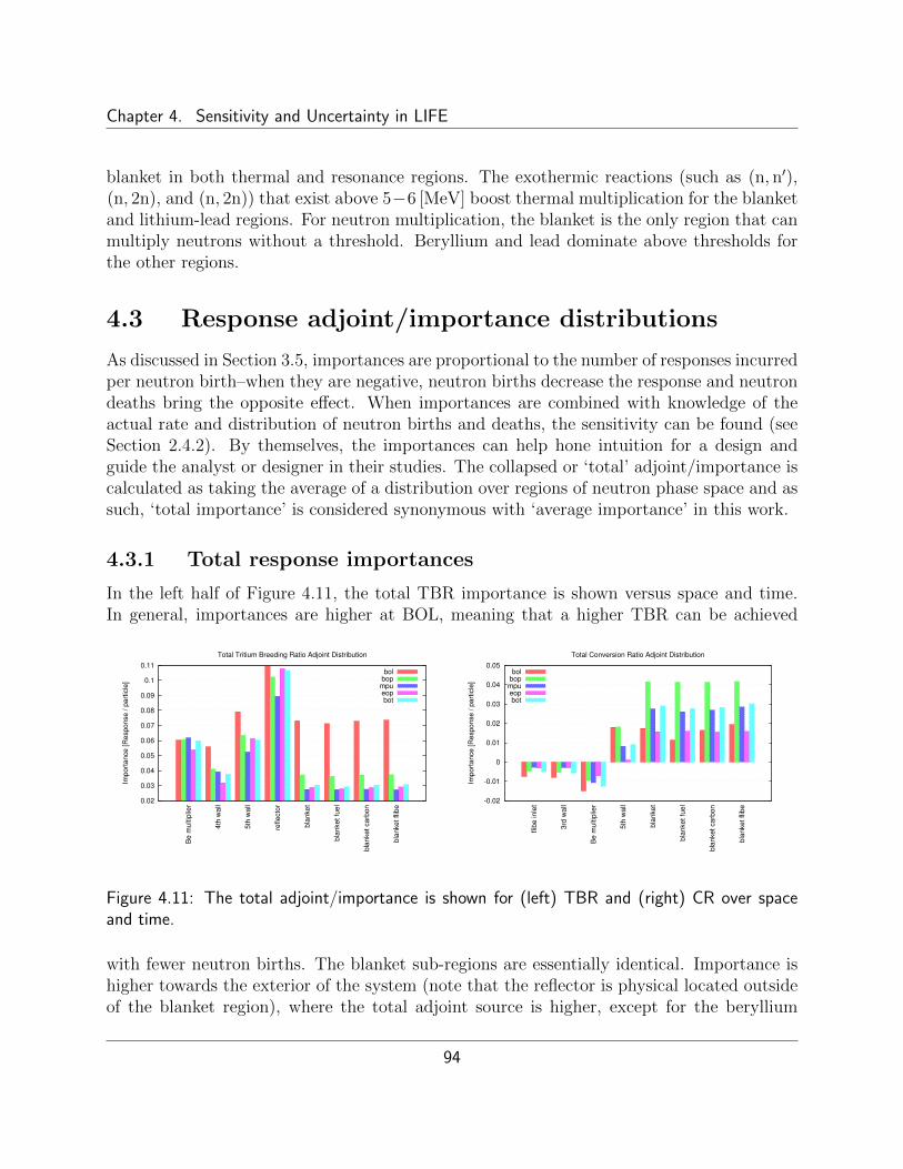
Chapter 4. Sensitivity and Uncertainty in LIFE
blanket in both thermal and resonance regions. The exothermic reactions (such as (n, n′),(n, 2n), and (n, 2n)) that exist above 5−6 [MeV] boost thermal multiplication for the blanketand lithium-lead regions. For neutron multiplication, the blanket is the only region that canmultiply neutrons without a threshold. Beryllium and lead dominate above thresholds forthe other regions.
4.3 Response adjoint/importance distributions
As discussed in Section 3.5, importances are proportional to the number of responses incurredper neutron birth–when they are negative, neutron births decrease the response and neutrondeaths bring the opposite effect. When importances are combined with knowledge of theactual rate and distribution of neutron births and deaths, the sensitivity can be found (seeSection 2.4.2). By themselves, the importances can help hone intuition for a design andguide the analyst or designer in their studies. The collapsed or ‘total’ adjoint/importance iscalculated as taking the average of a distribution over regions of neutron phase space and assuch, ‘total importance’ is considered synonymous with ‘average importance’ in this work.
4.3.1 Total response importances
In the left half of Figure 4.11, the total TBR importance is shown versus space and time.In general, importances are higher at BOL, meaning that a higher TBR can be achieved
0.02
0.03
0.04
0.05
0.06
0.07
0.08
0.09
0.1
0.11
Be m
ultip
lier
4th
wall
5th
wall
reflecto
r
bla
nket
bla
nket fu
el
bla
nket carb
on
bla
nket flib
e
Import
ance [R
esponse / p
art
icle
]
Total Tritium Breeding Ratio Adjoint Distribution
bolbopmpueopbot
-0.02
-0.01
0
0.01
0.02
0.03
0.04
0.05
flib
e inle
t
3rd
wall
Be m
ultip
lier
5th
wall
bla
nket
bla
nket fu
el
bla
nket carb
on
bla
nket flib
e
Import
ance [R
esponse / p
art
icle
]
Total Conversion Ratio Adjoint Distribution
bolbopmpueopbot
Figure 4.11: The total adjoint/importance is shown for (left) TBR and (right) CR over spaceand time.
with fewer neutron births. The blanket sub-regions are essentially identical. Importance ishigher towards the exterior of the system (note that the reflector is physical located outsideof the blanket region), where the total adjoint source is higher, except for the beryllium
94

Chapter 4. Sensitivity and Uncertainty in LIFE
multiplier, which has the opportunity to generate excess particles through (n, 2n) reactions.As thermally absorptive fission products build up in the blanket, the importance of theblanket in producing tritium decreases.
The right half of Figure 4.11 shows the total CR importance versus space and time.Importance is generally negative towards the interior and positive towards the exterior.This is because neutrons towards the interior of the blanket have to pass through manycentimeters of moderator before encountering the blanket, upon which they will be thermaland more likely to fission than breed (breeding is primarily done with radiative capture inthe resonance energies). Importance in the blanket peaks at BOP, drops down to bottomout at EOP, and then jumps up to an intermediate value at BOT. This oscillatory behavioris seen again in the thermal multiplication importance.
Figure 4.12, the total importance is shown versus space and time for both varieties ofblanket multiplication. The blanket and its containing walls possess the highest importance,
0
0.02
0.04
0.06
0.08
0.1
0.12
0.14
0.16
flib
e inle
t
3rd
wall
Be m
ultip
lier
4th
wall
5th
wall
reflecto
r
bla
nket
bla
nket fu
el
bla
nket carb
on
bla
nket flib
e
Import
ance [R
esponse / p
art
icle
]
Total Thermal Multiplication Adjoint Distribution
bolbopmpueopbot
0
0.001
0.002
0.003
0.004
0.005
0.006
0.007
fusio
n c
ham
ber
tungste
n a
rmor
1st w
all
lithiu
m-lead
2nd w
all
flib
e inle
t
3rd
wall
Be m
ultip
lier
4th
wall
5th
wall
reflecto
r
bla
nket
bla
nket fu
el
bla
nket carb
on
bla
nket flib
e
Import
ance [R
esponse / p
art
icle
]Total Neutron Multiplication Adjoint Distribution
bolbopmpueopbot
Figure 4.12: The total adjoint/importance is shown for (left) Mth and (right) Mn over space andtime.
followed by the beryllium multiplier. The reflector is least important in terms of thermaland neutron multiplication. The time-oscillation of thermal multiplication can be explainedas a combination of the accumulation of fission products and the accumulation of fissile fuel–a downward concave hump. This is the same shape as the 6Li enrichment time evolution(Figure 4.2). The jump in thermal multiplication from EOP to BOT is due to the increase inthe 6Li enrichment, which increases the adjoint source for the exothermic 6Li(n,T) reaction.At the same time, this adjustment suppresses fission reactions and thus decreases neutronmultiplication importance throughout.
95

Chapter 4. Sensitivity and Uncertainty in LIFE
4.3.2 Response importance energy distributions
Adjoint/importance distributions are also useful when viewed as a function of neutron kineticenergy. In this form, they show how possible neutron source and sink spectra could be tunedto optimize a response. In Figure 4.13, the importance spectra are shown for TBR at BOLand MPU. In general, importance is larger at thermal energies for BOL, while thermal
0
0.02
0.04
0.06
0.08
0.1
0.12
0.14
10-8
10-7
10-6
10-5
10-4
10-3
10-2
10-1
100
101
Import
ance [R
esponse / p
art
icle
]
Energy [MeV]
Beginning of Life Tritium Breeding Ratio Adjoint Distribution
Be multiplier4th wall5th wallreflectorblanket
blanket fuelblanket carbon
blanket flibe 0
0.02
0.04
0.06
0.08
0.1
0.12
10-8
10-7
10-6
10-5
10-4
10-3
10-2
10-1
100
101
Import
ance [R
esponse / p
art
icle
]
Energy [MeV]
Maximum Plutonium Mass Tritium Breeding Ratio Adjoint Distribution
lithium-lead2nd wallflibe inlet3rd wall
Be multiplier4th wall5th wallreflector
Figure 4.13: The adjoint/importance distribution is shown for TBR at (left) BOL and (right)MPU.
importances are decreased by absorptive fission products at thermal energies for MPU. Thereflector has the largest importance over the entire spectrum. There are very dramaticjumps in importance within the beryllium multiplier region due to 9Be(n, 2n) reactions.Within characteristic resonances in 238U and 56Fe, there are sharp drops in importances.These resonances capture neutrons and represent a barrier of faster neutrons from reachingthermal energies where they can breed tritium.
Figure 4.14 contains the CR adjoint distributions for BOL and MPU. The spectra arenegative at low energies and positive at high energies. This is because fission tends to occurat thermal energies and radiative capture breeding tends to occur within resonance and fastenergies. The 238U resonances that depressed the TBR importance in Figure 4.13 are positivejumps in the CR importance. The reflector and beryllium multiplier regions, which have theutility to serve as moderators and multipliers, are positive at high energies, where they tendto push neutrons to resonance energies, and negative at low energies, where they tend topush neutrons out of resonance regions and into thermal energies.
The multiplier importance distributions at BOL are shown in Figure 4.15 below. Forthermal multiplication, the blanket is most important. Multiplication is most important athigh energies. This is where the cross-sections for (n, 2n) and (n, 3n) exist. For neutronmultiplication, importance generally decreases outwards from the lithium-lead region to theberyllium multiplier region. The fusion chamber contains leaked importance from the neigh-
96

Chapter 4. Sensitivity and Uncertainty in LIFE
-0.2
-0.15
-0.1
-0.05
0
0.05
0.1
0.15
0.2
10-8
10-7
10-6
10-5
10-4
10-3
10-2
10-1
100
101
Import
ance [R
esponse / p
art
icle
]
Energy [MeV]
Beginning of Life Conversion Ratio Adjoint Distribution
Be multiplier4th wall5th wallreflectorblanket
blanket fuelblanket carbon
blanket flibe-0.2
-0.1
0
0.1
0.2
0.3
10-8
10-7
10-6
10-5
10-4
10-3
10-2
10-1
100
101
Import
ance [R
esponse / p
art
icle
]
Energy [MeV]
Maximum Plutonium Mass Conversion Ratio Adjoint Distribution
Be multiplier4th wall5th wallreflectorblanket
blanket fuelblanket carbon
blanket flibe
Figure 4.14: The adjoint/importance distribution is shown for CR at (left) BOL and (right) MPU.
0
0.02
0.04
0.06
0.08
0.1
0.12
0.14
10-8
10-7
10-6
10-5
10-4
10-3
10-2
10-1
100
101
Import
ance [R
esponse / p
art
icle
]
Energy [MeV]
Beginning of Life Thermal Multiplication Adjoint Distribution
Be multiplier4th wall5th wallblanket
blanket fuelblanket carbon
blanket flibe 0
0.01
0.02
0.03
0.04
0.05
0.06
0.07
0 2 4 6 8 10 12 14
Import
ance [R
esponse / p
art
icle
]
Energy [MeV]
Beginning of Life Neutron Multiplication Adjoint Distribution
fusion chambertungsten armor
1st walllithium-lead
2nd wallflibe inlet3rd wall
Be multiplier
Figure 4.15: The adjoint/importance distribution is shown at BOL for (left) Mth and (right) Mn.
boring inner regions. The first, second, and third wall are highly important, while the moreouter walls did not meet the threshold requirements for visibility on this graph.
4.3.3 Response importance angular distributions
The direction a particle travels is often important. For example, a particle located near theperiphery of a system is less likely to collide and cause a response when it is heading outwardsthan when it is heading inwards. Because of this, adjoint/importance angular distributionsare often anisotropic near geometrical features like boundaries and absorbers. Figure 4.16shows the angular distribution (for each energy bin) of TBR importance within two spatialregions at MPU. The lithium-lead region resides towards the center of the system and isbombarded with adjoint particles somewhat isotropically. Additionally, it is the source ofa portion of the adjoint source. Consequently, its distribution is somewhat isotropic. The
97

Chapter 4. Sensitivity and Uncertainty in LIFE
10−8
10−7
10−6
10−5
10−4
10−3
10−2
10−1
100
101
−1
−0.75
−0.5
−0.25
0
0.25
0.5
0.75
1
Lithium−Lead Adjoint/Importance Angular Distribution
Neutron Energy [MeV]
Angula
r C
osin
e µ
0
0.1
0.2
0.3
0.4
0.5
0.6
0.7
0.8
0.9
1
10−8
10−7
10−6
10−5
10−4
10−3
10−2
10−1
100
101
−1
−0.75
−0.5
−0.25
0
0.25
0.5
0.75
1
Blanket Adjoint/Importance Angular Distribution
Neutron Energy [MeV]
Angula
r C
osin
e µ
0
0.1
0.2
0.3
0.4
0.5
0.6
0.7
0.8
0.9
1
Figure 4.16: The TBR adjoint/importance angular distribution for MPU within (left) the lithium-lead region and (right) the blanket. Particles with a cosine of positive one are travelling outwardsand particles with a cosine of negative one are travelling inwards.
only anomaly (one that forbids separability of angular dependence from spatial and energydependence) is that importance at low energies preferentially heads inwards. The blanketis a different matter; its importance angular distribution is quite anisotropic. The blanketis located towards the extremity of the design and accordingly, particles that travel inwardsare somewhat more important than those travelling outwards.
4.4 Sensitivity analysis
For some, sensitivities are the end of the line–the sought after result of a sensitivity analysis.Sensitivities possess none of the limitations of the metrics shown and discussed in the previoussections. Adjoint source distributions (Figures 4.8, 4.9, and 4.10) represent the capacity ofa material to contribute to a response, but speak nothing of the neutron spectrum or thegeometrical arrangement of materials. Total adjoint sources (Figures 4.6 and 4.7) incorporatethe former, but not the latter. Total adjoint/importances (Figures 4.11 and 4.12)–the resultsof adjointly transporting adjoint sources within the system geometry–show the smearedaverage of importance over a spatial region without regard to the distribution of neutronsources and sinks. Adjoint/importance distributions (Figures 4.13, 4.14, and 4.15) are un-collapsed and therefore allow for detailed study, but still do not take into consideration theneutron sources and sinks. Only after they are considered by way of constructing the adjointbilinear functional (see Section 3.2) is the sensitivity found.
Sensitivities quantify the linear relative change in a response with respect to a relative
98

Chapter 4. Sensitivity and Uncertainty in LIFE
perturbation in an input parameter (see Section 2.3). Explicit sensitivities discount the effectof any perturbation upon the flux, holding it constant. The more physical implicit sensitivityconsiders the effect of any perturbation upon the flux, to first order. Consequently, explicitsensitivities for responses due to most input perturbations are zero (many inputs are notexplicitly related to a given response) and in contrast, implicit sensitivities of responses toany input (for which flux perturbations are expressly considered) are usually non-zero.
Response sensitivities sum up to one of two values: sensitivities for linear functional re-sponses like TBR, Mth, and Mn add up to one; sensitivities for linear function ratio responseslike CR add up to zero. For clarity of presentation, lesser sensitivities–bins for which thesensitivity is below a certain threshold–are removed from graphs. Consequently, the grandtotal of sensitivities for the following graphs may not add up conservatively.
4.4.1 Comparison of implicit and explicit sensitivities
The left half of Figure 4.17 compares total implicit and explicit sensitivities for TBR atMPU to isotopic reaction rates. While 56Fe, 238U, and 239Pu do not explicitly participate
-10%
0%
10%
20%
30%
40%
50%
60%
70%
80%
90%
100%
za 3
006
za 3
007
za 4
009
za 2
6056
za 9
2238
za 9
4239
Implic
it-S
ensitiv
ity
Maximum Plutonium Mass Tritium Breeding Ratio Implicit Versus Explicit Sensitivity
implicitexplicit
-5%
0%
5%
10%
15%
20%
25%
30%
35%
40%
45%
50%
za 3
006
za 3
007
za 2
4053
za 2
6056
za 7
4182
za 7
4183
za 7
4186
za 8
2206
za 8
2207
za 8
2208
za 9
2238
za 9
4239
za 9
4241
za 9
6245
za 9
6247
Implic
it-S
ensitiv
ity
End of Plateau Thermal Multiplication Implicit Versus Explicit Sensitivity
implicitexplicit
Figure 4.17: Comparison of total implicit and explicit sensitivities for (left) TBR at MPI and(right) Mth and EOP.
in the production or destruction tritons, their presence implicitly eliminates neutrons thatcould otherwise breed tritium; the explicit sensitivity to their concentrations is zero andthe implicit sensitivity to their concentrations is negative. 6Li and 7Li breed tritium, butdoing so removes neutrons from the system; their explicit sensitivities are positive and theirimplicit sensitivities are slightly smaller. 9Be produces 0.9% of tritons at MPU, so its explicitsensitivity is 0.9%. However, 9Be(n, 2n) reactions also generate excess neutrons that caneventually produce tritium, so its implicit sensitivity is somewhat higher (2.5%).
The right half of Figure 4.17 compares total implicit and explicit sensitivities for Mth
at EOP and its story somewhat is similar to TBR total sensitivities at MPU. Isotopes that
99

Chapter 4. Sensitivity and Uncertainty in LIFE
participate in exothermic nuclear reactions (6Li, 56Fe, 238U, 249Pu, 241Pu, 245Cm, and 247Cm),exhibit positive explicit sensitivities to thermal multiplication; their implicit sensitivitiesare also positive, but less so since their presence depresses neutrons and their ability toparticipate in other thermal multiplication. Thermal multiplication is explicitly negativelysensitive to isotopes that participate in endothermic nuclear reactions (7Li and 206−208Pb);it is implicitly slightly more negatively sensitive to those same isotopes because they thereactions parasitically absorb neutrons.
4.4.2 Total sensitivities
Sensitivities can be collapsed and distributed over a number of parameters according to theanalysis. When they are collapsed over all but cells, they represent the spatial variation ofsensitivity in a design. When they are collapsed over all but isotope, they represent thesensitivity of responses to those isotopic number densities. When they are collapsed overall but reaction type, they show how different reactions participate in causing a response.When they are collapsed over all but cells and isotopes, they show how the spatial variationof isotopic number densities affect a response. This can be especially useful for optimizationof responses [Vujic et al., 2003]. When they are collapsed over all but cells and reactiontypes, they show how different reactions affect a response spatially. When they are collapsedover all but isotope and reaction type, they quantify the influence of each isotope’s reactionupon the response. This collapsing scheme is appropriate when propagating nuclear datauncertainties for the reactions of certain isotopes. When sensitivities are not collapsed at all,they show how isotopic reactions affect a response versus space. This most detailed binningof sensitivities offers the analyst a rich set of information with which to garner insight for adesign.
The spatial distribution of neutron multiplication sensitivities are shown over time in theleft half of Figure 4.18. At BOL, when the blanket contains all fertile heavy metals and nofissile materials, it contributes only 5.9% of sensitivity to neutron multiplication while thelithium-lead region and beryllium multiplier contribute 19% and 67%, respectively. Afterthe blanket has had a chance to breed fissile materials, it jumps to around 30% of neutronmultiplication, reducing the lithium-lead and beryllium multiplier regions to around 14%and 50%, respectively. In spite of their parasitic absorption, structures generally contributeslightly positively to neutron multiplication. The right half of Figure 4.18 distributes thesame sensitivities over isotope (note the reverse order of timesteps), showing that 9Be isthe king of multiplication, followed by 239Pu, 241Pu, and 208−206Pb. The same sensitivitiesare finally shown distributed over reaction type in the left half of Figure 4.19, for intuitiveresults. (n, 2n) is responsible for the lions share of neutron multiplication throughout thelifetime, with a dip during the power plateau when the blanket can sustain ample fissions.
The right half of Figure 4.19 shows the sensitivity of TBR to various reaction types.Intuitively, tritium production is almost 100% sensitive to (n,T) reactions throughout the
100
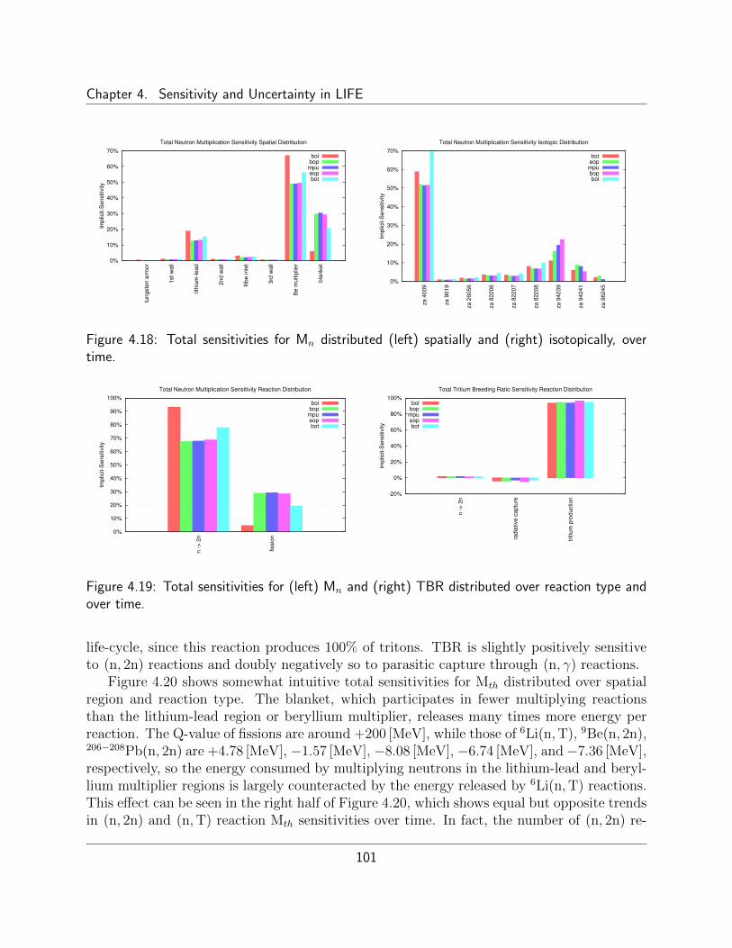
Chapter 4. Sensitivity and Uncertainty in LIFE
0%
10%
20%
30%
40%
50%
60%
70%tu
ngste
n a
rmor
1st w
all
lithiu
m-lead
2nd w
all
flib
e inle
t
3rd
wall
Be m
ultip
lier
bla
nket
Implic
it-S
ensitiv
ity
Total Neutron Multiplication Sensitivity Spatial Distribution
bolbopmpueopbot
0%
10%
20%
30%
40%
50%
60%
70%
za 4
009
za 9
019
za 2
6056
za 8
2206
za 8
2207
za 8
2208
za 9
4239
za 9
4241
za 9
6245
Implic
it-S
ensitiv
ity
Total Neutron Multiplication Sensitivity Isotopic Distribution
boteopmpubopbol
Figure 4.18: Total sensitivities for Mn distributed (left) spatially and (right) isotopically, overtime.
0%
10%
20%
30%
40%
50%
60%
70%
80%
90%
100%
n -
> 2
n
fissio
n
Implic
it-S
ensitiv
ity
Total Neutron Multiplication Sensitivity Reaction Distribution
bolbopmpueopbot
-20%
0%
20%
40%
60%
80%
100%
n -
> 2
n
radia
tive c
aptu
re
tritiu
m p
roduction
Implic
it-S
ensitiv
ity
Total Tritium Breeding Ratio Sensitivity Reaction Distribution
bolbopmpueopbot
Figure 4.19: Total sensitivities for (left) Mn and (right) TBR distributed over reaction type andover time.
life-cycle, since this reaction produces 100% of tritons. TBR is slightly positively sensitiveto (n, 2n) reactions and doubly negatively so to parasitic capture through (n, γ) reactions.
Figure 4.20 shows somewhat intuitive total sensitivities for Mth distributed over spatialregion and reaction type. The blanket, which participates in fewer multiplying reactionsthan the lithium-lead region or beryllium multiplier, releases many times more energy perreaction. The Q-value of fissions are around +200 [MeV], while those of 6Li(n,T), 9Be(n, 2n),206−208Pb(n, 2n) are +4.78 [MeV], −1.57 [MeV], −8.08 [MeV], −6.74 [MeV], and−7.36 [MeV],respectively, so the energy consumed by multiplying neutrons in the lithium-lead and beryl-lium multiplier regions is largely counteracted by the energy released by 6Li(n,T) reactions.This effect can be seen in the right half of Figure 4.20, which shows equal but opposite trendsin (n, 2n) and (n,T) reaction Mth sensitivities over time. In fact, the number of (n, 2n) re-
101

Chapter 4. Sensitivity and Uncertainty in LIFE
-10%
0%
10%
20%
30%
40%
50%
60%
70%
80%tu
ngste
n a
rmor
1st w
all
lithiu
m-lead
2nd w
all
3rd
wall
Be m
ultip
lier
4th
wall
reflecto
r
bla
nket
Implic
it-S
ensitiv
ity
Total Thermal Multiplication Sensitivity Spatial Distribution
bolbopmpueopbot
-40%
-20%
0%
20%
40%
60%
80%
100%
n -
> 2
n
fissio
n
radia
tive c
aptu
re
tritiu
m p
roduction
Implic
it-S
ensitiv
ity
Total Thermal Multiplication Sensitivity Reaction Distribution
bolbopmpueopbot
Figure 4.20: Total sensitivities for Mth distributed (left) spatially and (right) over reaction type,over time.
actions isn’t decreasing, only its relative sensitivity, as blanket fission increases. Thermalmultiplication is approximately equally sensitive to radiative capture and tritium productionthroughout life. The two are also responsible for 38% and 33% of sensitivity respectively,compared to fission’s 44% at BOL.
4.4.3 Sensitivity energy distributions
Like the previously discussed metrics, sensitivities offer a rich abundance of informationwhen they are distributed versus neutron kinetic energy. They can declare whether a systemis ‘fast’ or ‘thermal,’ by quantifying the fraction of sensitivity present in different energyregions. They can show the effect of the spatial change of neutron spectrum spatially on aresponse. They can be used to propagate energy-dependent nuclear data uncertainties toresponse uncertainties. In general, they offer another realm for the analyst to investigate intheir study of a design. Because logarithmic scales can span only positive or negative values,positive and negative sensitivities are split into their own graphs.
Figure 4.21 shows the sensitivity energy distributions for TBR at BOL for various isotopicreaction types. The sensitivity is largest for 6Li(n,T) at the thermal hump. 7Li(n,T) and9Be(n, 2n) are the second largest at energies above their thresholds–3−4 orders of magnitudehigher than that of 6Li(n,T) in the same energy range. 56Fe(n, γ) and 238U(n, γ) take awayaround 1% of TBR sensitivity within resonance regions.
Figure 4.22 shows the sensitivity energy distributions for Mth at MPU for various iso-topic reaction types. 239Pu(n, fission), 241Pu(n, fission), 245Cm(n, fission), 6Li(n,T), and238U(n, fission) contribute the largest to thermal multiplication sensitivity. The first threeare essentially distributed evenly over fast, resonance, and thermal energy regions. The plu-toniums’ thermal resonances are very prominent on the thermal hump. The fourth reaction
102
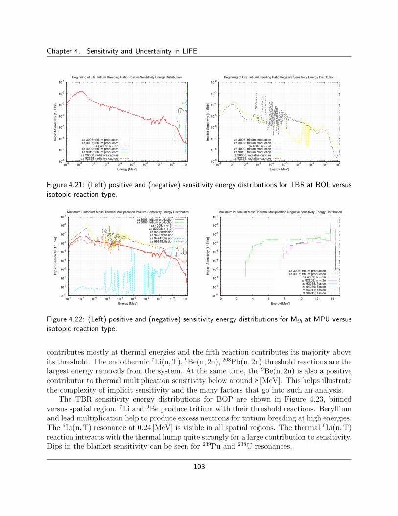
Chapter 4. Sensitivity and Uncertainty in LIFE
10-8
10-7
10-6
10-5
10-4
10-3
10-2
10-1
10-8
10-7
10-6
10-5
10-4
10-3
10-2
10-1
100
101
Implic
it-S
ensitiv
ity [1 / E
bin
]
Energy [MeV]
Beginning of Life Tritium Breeding Ratio Positive Sensitivity Energy Distribution
za 3006; tritium productionza 3007; tritium production
za 4009; n -> 2nza 4009; tritium productionza 9019; tritium production
za 26056; radiative captureza 92238; radiative capture
10-9
10-8
10-7
10-6
10-5
10-4
10-3
10-2
10-8
10-7
10-6
10-5
10-4
10-3
10-2
10-1
100
101
Implic
it-S
ensitiv
ity [1 / E
bin
]
Energy [MeV]
Beginning of Life Tritium Breeding Ratio Negative Sensitivity Energy Distribution
za 3006; tritium productionza 3007; tritium production
za 4009; n -> 2nza 4009; tritium productionza 9019; tritium production
za 26056; radiative captureza 92238; radiative capture
Figure 4.21: (Left) positive and (negative) sensitivity energy distributions for TBR at BOL versusisotopic reaction type.
10-10
10-9
10-8
10-7
10-6
10-5
10-4
10-3
10-2
10-1
10-8
10-7
10-6
10-5
10-4
10-3
10-2
10-1
100
101
Implic
it-S
ensitiv
ity [1 / E
bin
]
Energy [MeV]
Maximum Plutonium Mass Thermal Multiplication Positive Sensitivity Energy Distribution
za 3006; tritium productionza 3007; tritium production
za 4009; n -> 2nza 82208; n -> 2nza 92238; fissionza 94239; fissionza 94241; fissionza 96245; fission
10-10
10-9
10-8
10-7
10-6
10-5
10-4
10-3
10-2
10-1
0 2 4 6 8 10 12 14
Implic
it-S
ensitiv
ity [1 / E
bin
]
Energy [MeV]
Maximum Plutonium Mass Thermal Multiplication Negative Sensitivity Energy Distribution
za 3006; tritium productionza 3007; tritium production
za 4009; n -> 2nza 82208; n -> 2nza 92238; fissionza 94239; fissionza 94241; fissionza 96245; fission
Figure 4.22: (Left) positive and (negative) sensitivity energy distributions for Mth at MPU versusisotopic reaction type.
contributes mostly at thermal energies and the fifth reaction contributes its majority aboveits threshold. The endothermic 7Li(n,T), 9Be(n, 2n), 208Pb(n, 2n) threshold reactions are thelargest energy removals from the system. At the same time, the 9Be(n, 2n) is also a positivecontributor to thermal multiplication sensitivity below around 8 [MeV]. This helps illustratethe complexity of implicit sensitivity and the many factors that go into such an analysis.
The TBR sensitivity energy distributions for BOP are shown in Figure 4.23, binnedversus spatial region. 7Li and 9Be produce tritium with their threshold reactions. Berylliumand lead multiplication help to produce excess neutrons for tritium breeding at high energies.The 6Li(n,T) resonance at 0.24 [MeV] is visible in all spatial regions. The thermal 6Li(n,T)reaction interacts with the thermal hump quite strongly for a large contribution to sensitivity.Dips in the blanket sensitivity can be seen for 239Pu and 238U resonances.
103

Chapter 4. Sensitivity and Uncertainty in LIFE
10-9
10-8
10-7
10-6
10-5
10-4
10-3
10-2
10-1
10-8
10-7
10-6
10-5
10-4
10-3
10-2
10-1
100
101
Imp
licit-S
en
sitiv
ity [
1 /
Eb
in]
Energy [MeV]
Beginning of Plateau Tritium Breeding Ratio Sensitivity Energy Distribution
lithium-leadflibe inlet
Be multiplierreflectorblanket
Figure 4.23: Sensitivity energy distributions for TBR at BOP versus spatial region.
The BOP Mn sensitivity energy distributions are shown in Figure 4.24, binned versusspatial region. The blanket provides most of its multiplication sensitivity at thermal and
10-7
10-6
10-5
10-4
10-3
10-2
10-1
100
10-8
10-7
10-6
10-5
10-4
10-3
10-2
10-1
100
101
Implic
it-S
ensitiv
ity [1 / E
bin
]
Energy [MeV]
Beginning of Plateau Neutron Multiplication Positive Sensitivity Energy Distribution
lithium-leadflibe inlet
Be multiplierblanket
10-9
10-8
10-7
10-6
10-5
10-4
10-3
10-8
10-7
10-6
10-5
10-4
10-3
10-2
10-1
100
101
Implic
it-S
ensitiv
ity [1 / E
bin
]
Energy [MeV]
Beginning of Plateau Neutron Multiplication Negative Sensitivity Energy Distribution
lithium-leadflibe inlet
Be multiplierblanket
Figure 4.24: (Left) positive and (negative) sensitivity energy distributions for Mn at BOP versusspatial region.
resonance energies upon Pu(n, fission) reactions. The beryllium multiplier provides its mul-tiplication at high energies, where the 9Be(n, 2n) reaction is present. The lithium-lead and
104

Chapter 4. Sensitivity and Uncertainty in LIFE
flibe inlet regions provide the slightest bit of multiplication at energies above (n, 2n) thresh-olds. The beryllium multiplier, lithium-lead, and flibe inlet regions are strong absorbers atresonance and thermal energies. This is where neutrons are sacrificed for the breeding oftritium.
The MPU CR sensitivity energy distributions are shown in Figure 4.25, binned versusspatial region. This blanket destroys fissile fuel at thermal energies, does a mix of fuel
10-9
10-8
10-7
10-6
10-5
10-4
10-3
10-2
10-1
100
10-8
10-7
10-6
10-5
10-4
10-3
10-2
10-1
100
101
Implic
it-S
ensitiv
ity [1 / E
bin
]
Energy [MeV]
Maximum Plutonium Mass Conversion Ratio Positive Sensitivity Energy Distribution
Be multiplierblanket
10-10
10-9
10-8
10-7
10-6
10-5
10-4
10-3
10-2
10-1
10-8
10-7
10-6
10-5
10-4
10-3
10-2
10-1
100
101
Implic
it-S
ensitiv
ity [1 / E
bin
]
Energy [MeV]
Maximum Plutonium Mass Conversion Ratio Negative Sensitivity Energy Distribution
Be multiplierblanket
Figure 4.25: (Left) positive and (negative) sensitivity energy distributions for CR at MPU versusspatial region.
breeding and destruction within lower resonance regions, breeds within the upper resonanceregion, and destroys fuel again within the unresolved resonance and threshold energies. Theberyllium multiplier region steals neutrons from potential fissions at thermal energies, stealsneutrons that would thermalize somewhat and potentially breed in the blanket within upperresonance energies, steals neutrons from the unresolved resonance region that might fast-fission in the blanket, and provides a little bit of excess neutron production (and energyreduction) at threshold energies to enhance fast-fission.
4.5 Validation of adjoint-based methods
Two tests are performed in order to validated the sensitivity estimates of this work. In thefirst test, the number density of 6Li within the lithium-lead region of BOL is increased 5%from 2.992 × 10⁻⁴ → 3.142 × 10⁻⁴
[atoms
barn−cm
]. With the linear sensitivity coefficient of the
TBR response to this input estimated to be +28.5%, the TBR is predicted to increase by+1.43%. For the second test, the number density of 56Fe is decreased by 20% within allstructural regions of BOL: the 1st wall, 2nd wall, 3rd wall, 4th wall, 5th wall, and finalwall and decreasing their mass densities by almost the same amount. The linear sensitivitycoefficients of TBR to these inputs are−0.0375%, −0.0820%, −0.136%, −0.413%, −0.0242%,
105

Chapter 4. Sensitivity and Uncertainty in LIFE
−0.000982%, respectively, for a total linear sensitivity of −0.693% and a predicted changein TBR of +0.139%.
The unperturbed BOL TBR is calculated as 1.04071 ± 0.00009 (counting uncertainty).The TBR resulting from the 6Li perturbation is 1.05450 ± 0.00009. This represents anincrease of 1.33%, which is relatively 7.6% lower than the predicted increase of 1.43%: thecorrect direction and approximately the correct magnitude. The TBR resulting from the 56Feperturbation is 1.04415± 0.00009. This represents an increase of 0.331%, which is relatively58% higher than the predicted increase of 0.139%: the correct direction, but quite a differentmagnitude.
While the first test is considered to somewhat validate the adjoint-based sensitivities, thesecond test is considered less successful in this respect. The 20% change in the 56Fe densitywas necessary to bring a response change large enough to escape counting uncertainty noise.A 20% change in any input is a very large perturbation that likely lays outside the realmof linear sensitivity coefficient accuracy. Additionally, when the gross errors in resonantcapture in 56Fe within ENJEFF (see Section 3.8.4.3) are considered such a large discrepancyis almost to be expected.
4.6 Uncertainty analysis
In this section, estimates are made for the uncertainty of responses from three sources: (1)uncertain nuclear data; (2) statistical counting uncertainty of response estimates; and (3)statistical counting uncertainty of sensitivity estimates, which propagate to nuclear datauncertainty estimates–variances of variances. No restrictions were made in the uncertaintyanalysis. Every isotope present and each of their nuclear reactions are considered as sourcesof nuclear data uncertainty. Only at the very end, when uncertainty estimates are made, arethe unimportant sources thrown to the side–no isotopes were hand-picked and no nuclearreactions were ‘known’ to be important a priori.
Uncertainties can be communicated in a number of ways, for example as an absoluteuncertainty: 16 ± 2 [tangelos], a relative uncertainty: 16 [tangelos] ± 12.5%, or a confidenceinterval (the expected value minus and plus 2.58 standard deviations): “there is a 99% chancethat the number of tangelos lays between 10.8 and 21.2”. The uncertainty that an inputcontributes to a response can be reported and the intrinsic uncertainty of that input can bereported, irrespective of how sensitive that response is to the input. One can calculate theeffective intrinsic uncertainty of an input p (Up) by dividing the overall relative uncertaintythat an input contributes to a result R (UR,p) by the overall sensitivity that result has tothe input (SR,p):
Up =UR,pSR,p
, (4.1)
for example, an input that contributes 0.5% uncertainty to a response and 10% of the
106

Chapter 4. Sensitivity and Uncertainty in LIFE
sensitivity to that response has, itself, an effective 5% uncertainty. This single numberrepresents how uncertain an input is for the design and neutron spectrum the uncertaintyanalysis was performed for. More generally, nuclear data uncertainties vary with neutronkinetic energy (see Section 4.6.3).
4.6.1 Nuclear response uncertainty estimates
The uncertainty tables in this section contain seven columns. The first two identify thenuclear reaction input and the third and fourth report the reaction rate (per source neutron)and sensitivity of the response (detailed in the caption) to that input. The fifth and sixthcolumns report the relative uncertainty from nuclear data uncertainties (‘XS’) and statisticalcounting uncertainties (‘MC’), respectively with the units of pcm. One pcm is 10−5 or1%
1000or one ‘per-centi-milli.’ The seventh column shows the relative counting uncertainty
of the nuclear data uncertainty estimate (‘MCXS’), also in pcm. The cumulative row atthe bottom of each table contains the estimate of the response, plus and minus its overalluncertainty (from the three sources) and the relative uncertainty that each source contributesindividually, again in pcm.
Table 4.1 summarizes the most important contributors to BOL Mth uncertainty. The
Isotope Reaction Rate Sensitivity XS MC MC XS[rxn/s] [pcm] [pcm] [pcm]
U-235 (n,fission) 0.02434 40.19% 609.29 20.09 0.19Li-6 (n,T) 0.95380 37.52% 74.88 8.74 0.01
Fe-56 (n, γ) 0.20378 13.53% 652.65 3.27 2.66Be-9 (n, 2n) 0.60390 -7.50% 123.42 2.14 9.03
U-238 (n, γ) 0.20405 6.48% 82.56 3.89 0.24Pb-208 (n, 2n) 0.09014 -6.22% 345.21 1.24 180.95U-238 (n,fission) 0.00225 3.72% 24.53 3.35 0.05Pb-206 (n, 2n) 0.04078 -3.09% 188.91 0.62 98.61
Li-7 (n,T) 0.07315 -3.00% 274.04 0.82 81.70W-182 (n, γ) 0.05287 2.88% 252.11 2.20 8.31Pb-207 (n, 2n) 0.03820 -2.42% 132.26 0.48 74.07W-186 (n, γ) 0.04766 2.27% 66.81 1.26 1.06Be-9 (n, γ) 0.03861 2.25% 110.32 0.65 0.53Fe-56 (n, 2n) 0.01922 -2.02% 349.96 0.29 295.43W-183 (n, γ) 0.03007 1.99% 158.31 1.81 3.13
. . . . . . . . . . . . . . . . . . . . .
Cumulative 0.77280 ± 0.00957 1168.15 23.15 410.37
Table 4.1: Top uncertainties of Mth at BOL.
6Li(n,T), 9Be(n, 2n), 238U(n, γ), and 56Fe(n, γ) reactions occur the most frequently, but the
107

Chapter 4. Sensitivity and Uncertainty in LIFE
235U(n, fission) reaction contributes the most to sensitivity. The largest contributors to nu-clear data uncertainty, however, are 56Fe(n, γ), 235U(n, fission), 56Fe(n, 2n), and 208Pb(n, 2n),with effective uncertainties of 4.8%, 1.5%, 17%, and 5.6%. Of all reactions that contributemore than 0.1% of absolute sensitivity, 238U(n, 3n), 7Li(n, 2n), and 19F(n,T) have the highesteffective intrinsic uncertainties, with 38%, 34%, and 29% respectively. Statistical countinguncertainty is well bounded by nuclear data uncertainty, but the counting uncertainty of thenuclear data uncertainty is somewhat high. The uncertainty of Mth from all sources sums to1.2% at BOL, for a 99% confidence interval of 0.75− 0.78.
Table 4.2 contains the top uncertainties for TBR at BOP. The most frequent reactions are
Isotope Reaction Rate Sensitivity XS MC MC XS[rxn/s] [pcm] [pcm] [pcm]
Li-6 (n,T) 0.97393 86.75% 173.05 20.50 0.02Li-7 (n,T) 0.07509 6.51% 584.37 1.74 133.82Be-9 (n, 2n) 0.61647 1.82% 33.65 0.52 10.92Be-9 (n,T) 0.01041 0.89% 83.54 0.34 21.82Fe-56 (n, γ) 0.17800 -0.87% 41.99 0.20 2.52U-238 (n, γ) 0.35971 -0.78% 10.11 0.47 0.10Pu-239 (n,fission) 0.17783 -0.75% 5.92 0.45 0.04Pu-239 (n, γ) 0.10703 -0.53% 6.49 0.32 0.07Pu-240 (n, γ) 0.09078 -0.35% 7.19 0.28 0.45F-19 (n,T) 0.00332 0.29% 83.30 0.07 87.68Be-9 (n, γ) 0.03563 -0.24% 11.70 0.07 0.84Li-7 (n, γ) 0.03205 -0.20% 29.92 0.05 5.80
W-182 (n, γ) 0.05425 -0.18% 15.35 0.13 5.58W-186 (n, γ) 0.04788 -0.17% 5.13 0.10 1.37Pu-241 (n,fission) 0.04137 -0.17% 1.93 0.10 0.03
. . . . . . . . . . . . . . . . . . . . .
Cumulative 1.06273 ± 0.03569 624.42 20.60 3299.23
Table 4.2: Top uncertainties of TBR at BOP.
6Li(n,T), 9Be(n, 2n), 238U(n, γ), 56Fe(n, γ), 239Pu(n, fission), and 239Pu(n, γ) and those thatthe response is most sensitive to are 6Li(n,T), 7Li(n,T), 9Be(n, 2n), 9Be(n,T), and 56Fe(n, γ).The largest contributors to nuclear data uncertainty are 7Li(n,T), 6Li(n,T), 9Be(n,T), and19F(n,T), for effective intrinsic uncertainties of 9.0%, 0.20%, 9.4%, and 29%, respectively.The reactions that contribute more than 0.1% of absolute sensitivity with the highest ef-fective intrinsic uncertainty are 19F(n,T), 7Li(n, γ), 9Be(n,T), 7Li(n,T), and 182W(n, 102),with effective intrinsic uncertainties of 29%, 15%, 9.4%, 9.0%, and 8.6%. Statistical count-ing uncertainty is once again well bounded by nuclear data uncertainty, but the countinguncertainty of nuclear data uncertainty is 5× larger. This means that while the order ofmagnitude of the uncertainty estimate is likely correct, very few significant figures shouldbe trusted. The overall uncertainty of TBR from all sources (but mostly from counting
108

Chapter 4. Sensitivity and Uncertainty in LIFE
uncertainty of the nuclear data uncertainty) is 3.4% at BOP, for a 99% confidence intervalof 1.0− 1.2.
The top uncertainties for Mn at MPU are shown in Table 4.3 below. The reactions
Isotope Reaction Rate Sensitivity XS MC MC XS[rxn/s] [pcm] [pcm] [pcm]
Be-9 (n, 2n) 0.61871 51.49% 866.09 14.61 2.69Pu-239 (n,fission) 0.15420 19.52% 134.70 11.71 0.06Pu-241 (n,fission) 0.06383 8.09% 251.30 4.85 0.95Pb-208 (n, 2n) 0.09012 6.79% 375.57 1.36 36.77Pb-206 (n, 2n) 0.04077 3.07% 186.96 0.61 20.08Pb-207 (n, 2n) 0.03819 2.88% 156.45 0.58 15.09Fe-56 (n, 2n) 0.01922 1.47% 255.99 0.21 71.09
Cm-245 (n,fission) 0.00871 1.10% 63.33 0.66 0.08F-19 (n, 2n) 0.00940 0.75% 75.93 0.18 4.67Li-7 (n, 2n) 0.00502 0.40% 140.80 0.10 32.42
U-238 (n,fission) 0.00296 0.38% 2.33 0.26 0.00Li-7 (n,T) 0.07472 -0.27% 29.56 0.07 14.60
Pb-204 (n, 2n) 0.00233 0.18% 12.23 0.04 1.51Cr-52 (n, 2n) 0.00180 0.14% 28.48 0.02 17.95
Am-242 (n,fission) 0.00108 0.14% 9.73 0.10 0.03. . . . . . . . . . . . . . . . . . . . .
Cumulative 1.18160 ± 0.01261 1062.69 19.43 93.33
Table 4.3: Top uncertainties of Mn at MPU.
that the response is most sensitive to are among the most frequent reactions: 9Be(n, 2n),239Pu(n, fission), 241Pu(n, fission), 208Pb(n, 2n), and 206Pb(n, 2n). The largest contributorsto nuclear data uncertainty are the 9Be(n, 2n), 208Pb(n, 2n), 56Fe(n, γ), and 241Pu(n, fission)reactions, which have effective uncertainties of 1.7%, 5.5%, 17%, and 3.1%, respectively.The reactions with non-negligible sensitivity and the highest effective intrinsic uncertaintyare 7Li(n, 2n), 52Cr(n, 2n), 56Fe(n, 2n), and 19F(n, 2n), with values of 35%, 21%, 17%, and10%, respectively. Both flavors of counting uncertainty are well bounded by nuclear datauncertainty for this response, so the overall uncertainty estimate of 1.1% and estimated 99%confidence interval of 1.15− 1.21 can be trusted reasonably well.
Table 4.4 contains the top uncertainties for CR at EOP. The 238U(n, γ), 239Pu(n, fission),240Pu(n, γ), 239Pu(n, γ), and 240Pu(n, fission) reactions contribute the most to sensitivity.The 238U(n, γ), 240Pu(n, γ), 244Cm(n, γ), 241Pu(n, fission), 239Pu(n, fission), 239Pu(n, γ), and245Cm(n, fission) reactions contribute the most to nuclear data uncertainty, with effectiveintrinsic uncertainties of 1.3%, 2.1%, 4.4%, 1.5%, and 0.76%, respectively. The reactionsthat possess the largest effective intrinsic an non-negligible sensitivity are 247Cm(n, fission),155Eu(n, γ), 7Li(n,T), 243Am(n, γ), and 246Cm(n, γ), with values of 16%, 10%, 7.8%, 6.3%,5.8%, respectively. Counting uncertainty is well bounded by nuclear data uncertainty, but the
109

Chapter 4. Sensitivity and Uncertainty in LIFE
Isotope Reaction Rate Sensitivity XS MC MC XS[rxn/s] [pcm] [pcm] [pcm]
U-238 (n, γ) 0.17512 58.18% 740.27 40.73 1.72Pu-239 (n,fission) 0.12752 -37.17% 282.49 18.59 0.14Pu-240 (n, γ) 0.08519 28.60% 586.02 22.88 3.99Pu-239 (n, γ) 0.07664 -22.51% 261.37 11.26 0.24Pu-241 (n,fission) 0.06962 -20.44% 298.78 10.22 0.53Cm-244 (n, γ) 0.02348 7.83% 344.23 7.04 9.39Pu-241 (n, γ) 0.02577 -7.60% 96.67 3.80 0.10Cm-245 (n,fission) 0.02262 -6.65% 218.28 3.33 0.16Pu-238 (n, γ) 0.00627 2.17% 55.25 1.09 0.21Am-241 (n, γ) 0.00387 -1.14% 34.07 0.57 0.07Cm-245 (n, γ) 0.00338 -1.00% 39.86 0.50 0.05
Li-6 (n,T) 0.64414 0.86% 1.72 0.23 0.02Cm-246 (n, γ) 0.00147 0.49% 28.85 0.35 0.41Fe-56 (n, γ) 0.25548 0.44% 22.77 0.09 6.65
Cm-247 (n,fission) 0.00094 -0.28% 45.44 0.17 0.79. . . . . . . . . . . . . . . . . . . . .
Cumulative 0.88051 ± 0.03072 1146.68 53.25 3294.86
Table 4.4: Top uncertainties of CR at EOP.
counting uncertainty of nuclear data uncertainty is 3× larger. This means that perhaps onlyone significant figure of the uncertainty estimate can be trusted: 3.5% for a 99% confidenceinterval of 0.8− 1.0.
Top uncertainties for TBR at BOT are shown below in Table 4.5. Like with TBRat BOP, the most sensitive reactions are 6Li(n,T), 7Li(n,T), 9Be(n, 2n), 9Be(n,T), and56Fe(n, γ). Again, similarly to BOP, the largest contributors to nuclear data uncertaintyare the 7Li(n,T), 6Li(n,T), 9Be(n,T), and 19F(n,T), with effective intrinsic uncertaintiesof 9.1%, 0.20%, 9.4%, and 29%, respectively. The non-negligible reactions with the highesteffective intrinsic uncertainties are identical to BOP, except that the 182W(n, γ) reaction is8.8% instead of 8.6%.
Overall, the estimated nuclear data uncertainties of important figures of merit in LIFEwere quite moderate. The uncertainty in TBR remained below 1% for all time steps, stayingaround 0.6% for all time-steps except during EOP, when it was 0.9%. The CR uncertaintywas highest at BOL at 1.8% and fell to around 1.2% thereafter. The uncertainty for Mth
started at 1.2%, fell to around 0.6% at BOP, jumped up to 0.8% at MPU, and then fell backdown to 0.6% for EOP and BOT. The Mn uncertainty started at 1.4%, fell to 1% during thepower plateau, and then rose to 1.2% during BOT.
110

Chapter 4. Sensitivity and Uncertainty in LIFE
Isotope Reaction Rate Sensitivity XS MC MC XS[rxn/s] [pcm] [pcm] [pcm]
Li-6 (n,T) 0.95265 86.96% 173.35 20.56 0.02Li-7 (n,T) 0.07401 6.58% 596.17 1.78 113.77Be-9 (n, 2n) 0.61205 1.79% 32.71 0.51 9.02Be-9 (n,T) 0.01041 0.92% 85.72 0.35 18.18Fe-56 (n, γ) 0.14276 -0.68% 32.37 0.18 1.53F-19 (n,T) 0.00332 0.29% 85.40 0.08 74.50
Pu-239 (n,fission) 0.07561 -0.24% 1.89 0.14 0.01U-238 (n, γ) 0.12806 -0.22% 2.77 0.15 0.04Be-9 (n, γ) 0.02950 -0.19% 9.49 0.06 0.56
Pu-239 (n, γ) 0.04595 -0.18% 2.23 0.11 0.02Pu-240 (n, γ) 0.06142 -0.17% 3.51 0.16 0.16W-182 (n, γ) 0.04907 -0.16% 13.71 0.12 4.38W-186 (n, γ) 0.04281 -0.15% 4.62 0.09 1.08
Li-7 (n, γ) 0.02422 -0.15% 21.87 0.04 3.94Pu-241 (n,fission) 0.04114 -0.12% 1.24 0.07 0.02
. . . . . . . . . . . . . . . . . . . . .
Cumulative 1.04037 ± 0.19946 634.97 20.65 19161.73
Table 4.5: Top uncertainties of TBR at BOT.
4.6.2 Comparison of implicit and explicit uncertainty estimates
In Table 4.6, the explicit uncertainties of TBR at BOP are shown. This table, which has
Isotope Reaction Rate Sensitivity XS MC MC XS[rxn/s] [pcm] [pcm] [pcm]
Li-6 (n,T) 0.97393 91.64% 182.81 21.66 0.01Li-7 (n,T) 0.07509 7.07% 634.18 1.89 24.36Be-9 (n,T) 0.01041 0.98% 92.07 0.37 3.29F-19 (n,T) 0.00332 0.31% 91.09 0.08 10.66
Cumulative 1.06273 ± 0.00716 672.59 21.75 26.79
Table 4.6: Explicit uncertainties of TBR at BOP.
only four entries, should be viewed in the context of its implicit sibling Table 4.2. Explicitreaction rates and sensitivities are trivially related, with the latter equaling the individualcontributions to the sum of the former. 7Li(n,T) and 6Li(n,T) contribute the most touncertainty, with effective intrinsic uncertainties of 9.0% and 0.20%, each. The 9Be(n,T) and19F(n,T) intrinsic uncertainties remain essentially the same, but with TBR more explicitlysensitive to the reactions, the overall uncertainty estimate increases. These four isotopeswere the main players in the implicit uncertainty analysis. The nuclear data overwhelms
111

Chapter 4. Sensitivity and Uncertainty in LIFE
both varieties of counting uncertainty, so much trust is placed on the explicit nuclear datauncertainty estimate of 0.67%. This is 6× lower than the implicit sensitivity estimate.Consequently, the explicit 99% confidence interval is much tighter: 1.04− 1.08.
4.6.3 Intrinsic uncertainty of nuclear data
There are a few ways to represent the intrinsic uncertainty of nuclear data. The most intuitiveway, shown below in Figure 4.26, displays the expected value of the 6Li(n,T) microscopiccross-section in black and its range of possible values (plus and minus one standard deviation)in red. This relatively simple cross-section is the most important for TBR in the design (see
10-2
10-1
100
101
102
103
104
10-8
10-7
10-6
10-5
10-4
10-3
10-2
10-1
100
101
Mic
rosco
pic
Cro
ss-S
ectio
n [
ba
rns]
Neutron Energy [MeV]
Lithium-6 Tritium Production Cross-Section With Error Bounds
possible rangeexpected value
Figure 4.26: The 6Li tritium production cross-section has low uncertainty at thermal energies,but not insignificant uncertainty at high energies. Nominal nuclear data is courtesy of NADS[McKinley et al., 2004].
Tables 4.2 and 4.5). Since sensitivity to this cross-section is largest at thermal energies,where the uncertainty is quite low, the effective intrinsic uncertainty is also low.
The intrinsic uncertainty of nuclear data can also be shown as relative standard deviationsand correlation matrices, like in Figure 4.27 for 9Be(n, 2n). This threshold reaction is themost important for Mn in the design (see Table 4.3). Relative uncertainty is large at thethreshold and then 2− 3% above the threshold.
The covariance matrix for 56Fe(n, γ) is depicted below in Figure 4.28. This reaction is
112

Chapter 4. Sensitivity and Uncertainty in LIFE
1 2 3 4 5 6 7 8 9 10 11 12 13 14 15 16 17 18 19 200
5
10
15
20
25
9Be (n −> n + n) Uncertainty
Neutron Energy [MeV]
Re
lative
Un
ce
rta
inty
[%
]
1 2 3 4 5 6 7 8 9 10 11 12 13 14 15 16 17 18 19 201
2
3
4
5
6
7
8
9
10
11
12
13
14
15
16
17
18
19
20
Neutron Energy [MeV]
9Be (n −> n + n) Correlation Matrix
Ne
utr
on
En
erg
y [
Me
V]
0
0.1
0.2
0.3
0.4
0.5
0.6
0.7
0.8
0.9
1
Figure 4.27: The (left) relative uncertainty and (right) correlation matrix for 9Be(n, 2n). Covari-ances courtesy of [Little et al., 2008; DOE/NNSA, 2011].
10−11
10−10
10−9
10−8
10−7
10−6
10−5
10−4
10−3
10−2
10−1
100
101
0
10
20
30
40
50
60
56Fe (n −> γ) Uncertainty
Neutron Energy [MeV]
Rela
tive U
ncert
ain
ty [%
]
10−11
10−10
10−9
10−8
10−7
10−6
10−5
10−4
10−3
10−2
10−1
100
101
10−11
10−10
10−9
10−8
10−7
10−6
10−5
10−4
10−3
10−2
10−1
100
101
56Fe (n −> γ) Correlation Matrix
Neutron Energy [MeV]
Neutr
on E
nerg
y [M
eV
]
0
0.1
0.2
0.3
0.4
0.5
0.6
0.7
0.8
0.9
1
Figure 4.28: The (left) relative uncertainty and (right) correlation matrix for 26Fe(n, γ). Covari-ances courtesy of [Little et al., 2008; DOE/NNSA, 2011].
responsible for most of the parasitic absorption in the system and subsequently, most figuresof merit are negatively influenced by it (in a performance sense). At thermal and resonanceenergies, the uncertainty is estimated to be around 6% and around 12%. In the unresolvedregion, relative uncertainties climb to around 20% and then 30−50% in the threshold region.
Figure 4.29 shows the covariances for the 235U(n, fission) reaction. This reaction is respon-sible for a large amount of the thermal multiplication at BOL (see Table 4.1). Its overalluncertainty lays roughly between 1 − 2% for the entire energy spectrum except between
113

Chapter 4. Sensitivity and Uncertainty in LIFE
10−11
10−10
10−9
10−8
10−7
10−6
10−5
10−4
10−3
10−2
10−1
100
101
0
1
2
3
4
5
6
7
8
9
10
235U (n −> fission) Uncertainty
Neutron Energy [MeV]
Re
lative
Un
ce
rta
inty
[%
]
10−11
10−10
10−9
10−8
10−7
10−6
10−5
10−4
10−3
10−2
10−1
100
101
10−11
10−10
10−9
10−8
10−7
10−6
10−5
10−4
10−3
10−2
10−1
100
101
235U (n −> fission) Correlation Matrix
Neutron Energy [MeV]
Ne
utr
on
En
erg
y [
Me
V]
−1
−0.8
−0.6
−0.4
−0.2
0
0.2
0.4
0.6
0.8
1
Figure 4.29: The (left) relative uncertainty and (right) correlation matrix for 2U(n, 3)5fission.Covariances courtesy of [Shibata et al., 2011; JAEA/NDC, 2011b].
0.5− 10 [keV], where it jumps to 5%.The 238U(n, γ) reaction’s covariances are shown below in Figure 4.30. This resonance
10−11
10−10
10−9
10−8
10−7
10−6
10−5
10−4
10−3
10−2
10−1
100
101
0
5
10
15
20
25
30
35
40
45
50
55
238U (n −> γ) Uncertainty
Neutron Energy [MeV]
Rela
tive U
ncert
ain
ty [%
]
10−11
10−10
10−9
10−8
10−7
10−6
10−5
10−4
10−3
10−2
10−1
100
101
10−11
10−10
10−9
10−8
10−7
10−6
10−5
10−4
10−3
10−2
10−1
100
101
238U (n −> γ) Correlation Matrix
Neutron Energy [MeV]
Neutr
on E
nerg
y [M
eV
]
0
0.1
0.2
0.3
0.4
0.5
0.6
0.7
0.8
0.9
1
Figure 4.30: The (left) relative uncertainty and (right) correlation matrix for 238U(n, γ). Covari-ances courtesy of [Shibata et al., 2011; JAEA/NDC, 2011b].
reaction is responsible for most of the fertile breeding during the lifetime of the design (seeTable 4.4). The uncertainties within the range where sensitivities are highest are quite smallat around 1.3%. In the unresolved energy range, it jumps to 10%, then back below 5%. Atthreshold energies, the uncertainty is between 25− 50%, and lowest near the fusion neutron
114

Chapter 4. Sensitivity and Uncertainty in LIFE
energy of 14.08 [MeV].In Figure 4.31 below, effective intrinsic nuclear data uncertainties are plotted versus ex-
plicit sensitivity for all 2328 explicit sensitivities (binned by isotopic reaction type) generatedin this work. The overall negative correlation between the two implies that the less certain
10-4
10-3
10-2
10-1
100
10-12
10-11
10-10
10-9
10-8
10-7
10-6
10-5
10-4
10-3
10-2
10-1
100
101
Re
lative
Nu
cle
ar
Da
ta U
nce
rta
inty
Explicit Sensitivity
Correlation of Explicit Sensitivity and Nuclear Data Uncertainty
Figure 4.31: Effective intrinsic nuclear data uncertainty is negatively correlated with explicitsensitivity, with a correlation coefficient of -0.071 .
a nuclear datum is, the less explicitly sensitive the design is to it. It is expected that thiscorrelation coefficient is more negative for an LWR.
4.6.4 Comparison of nuclear data covariances and variances
In the occasional uncertainty analysis, a comparison is done between using full covariancematrices and using just the diagonal variances [Downar, 1991; Taiwo et al., 2005]. This workfollows their example by doing the same analysis, effectively changing Equation 2.1 from amatrix product to an element-wise product. By default, the full covariance matrices are used,but in order to determine how important off-diagonal terms are, a switch was programmedto allow for a comparison.
Table 4.7 shows the diagonal-only uncertainties of Mth at BOL. This table should bestudied alongside the ‘full-covariance’ version in Table 4.1. The overall nuclear data un-certainty is reduced. The 56Fe(n, 16), 208Pb(n, 16), 7Li(n, 205), 9Be(n, 16), 206Pb(n, 16),
115

Chapter 4. Sensitivity and Uncertainty in LIFE
Isotope Reaction Rate Sensitivity XS MC MC XS[rxn/s] [pcm] [pcm] [pcm]
U-235 (n,fission) 0.02434 40.20% 608.43 20.10 0.19Li-6 (n,T) 0.95380 37.52% 74.55 8.74 0.01
Fe-56 (n, γ) 0.20378 13.53% 652.16 3.27 2.66Be-9 (n, 2n) 0.60390 -7.39% 57.49 2.11 6.05
U-238 (n, γ) 0.20405 6.48% 82.55 3.89 0.24Pb-208 (n, 2n) 0.09014 -6.20% 254.70 1.24 158.98U-238 (n,fission) 0.00225 3.72% 12.73 3.35 0.05Pb-206 (n, 2n) 0.04078 -3.08% 139.87 0.62 85.46
Li-7 (n,T) 0.07315 -3.00% 196.48 0.82 69.49W-182 (n, γ) 0.05287 2.88% 252.03 2.20 8.31Pb-207 (n, 2n) 0.03820 -2.41% 97.52 0.48 64.56W-186 (n, γ) 0.04766 2.27% 66.79 1.26 1.06Be-9 (n, γ) 0.03861 2.25% 109.32 0.65 0.53Fe-56 (n, 2n) 0.01922 -2.01% 258.26 0.29 259.43W-183 (n, γ) 0.03007 1.99% 157.32 1.81 3.13
. . . . . . . . . . . . . . . . . . . . .
Cumulative 0.77280 ± 0.00879 1076.54 23.15 366.24
Table 4.7: Top ‘diagonal-only’ uncertainties of Mth at BOL.
9Be(n, 205), 207Pb(n, 16), 19F(n, 16), and 19F(n, 205) reactions all contribute 10’s of pcmless to nuclear data uncertainty. The effective intrinsic uncertainties are all reduced–on av-erage by a few percent. In general, the off-diagonal terms in covariance matrices increaseuncertainty estimates–by an amount that is not insignificant–and should not be left out inan uncertainty analysis.
4.6.5 Uncertainty associated with an imperfect uncertainty anal-ysis
In order to neglect one uncertainty among others, it should be at least 1 or 2 orders ofmagnitude smaller than the largest uncertainty. Otherwise, the total uncertainty will beerroneous by more than a percent or so (see Figure 4.32). In practice, one cannot argue thatan uncertainty or error is bounded by another until they are both quantified. Of course,once an uncertainty is quantified, it might as well be propagated.
Explicit sensitivities and explicit results uncertainties all have small counting uncertain-ties that are well bounded by nuclear data uncertainties. This is straightforward to achievesince relative counting uncertainty and explicit sensitivity are negatively correlated–regionsof phase space that a response is less explicitly sensitive to tend to be the regions that ‘see’fewer particles. For this same reason, the counting uncertainty of nuclear data estimates arenegatively correlated. Evidence for these trends are shown below in Figure 4.33. In these
116

Chapter 4. Sensitivity and Uncertainty in LIFE
10-3
10-2
10-1
100
101
102
0 0.5 1 1.5 2
Re
lative
Err
or
[%]
Orders of Magnitude Lesser of Smaller Uncertainty
Error Incurred by Neglecting Bounded Uncertainties
Figure 4.32: Penalty incurred by neglecting a smaller compounding uncertainty.
10-5
10-4
10-3
10-2
10-1
100
10-12
10-11
10-10
10-9
10-8
10-7
10-6
10-5
10-4
10-3
10-2
10-1
100
101
Sensitiv
ity R
ela
tive C
ounting E
rror
Explicit Sensitivity
Correlation of Explicit Sensitivity and Counting Error
10-9
10-8
10-7
10-6
10-5
10-4
10-3
10-2
10-1
100
10-12
10-11
10-10
10-9
10-8
10-7
10-6
10-5
10-4
10-3
10-2
10-1
100
101
Nucle
ar
Data
Uncert
ain
ty R
ela
tive C
ounting E
rror
Explicit Sensitivity
Correlation of Explicit Sensitivity and Nuclear Data Uncertainty Counting Error
Figure 4.33: Counting uncertainty and counting uncertainty of nuclear data uncertainty arenegatively correlated with explicit sensitivity, with correlation coefficients of -0.011 and -0.032,respectively.
graphs, both varieties of counting uncertainty are plotted against their associated explicitsensitivities for all 2328 explicit sensitivities that were calculated in this work. The inputsthat contribute the highest relative counting uncertainty to a response are associated withthe lowest sensitivity. Combining the two, absolute counting uncertainties remain small.
117

Chapter 4. Sensitivity and Uncertainty in LIFE
Errors associated with implicit sensitivity in this work are more complicated. For exam-ple, there are errors associated with multi-group cross-sections (see Section 3.8.4 and [Seifriedet al., 2011]). Several of the multi-group cross-sections are deemed inadequate for forwardtransport and therefore vicariously, so are some of the adjoint distributions. This is notaddressed fully. Additionally, due to computational restraints, adjoint distributions containa large degree of statistical counting uncertainty. This accounts for a large amount of thecounting uncertainty of implicit sensitivity estimates. Another large contributor to countinguncertainty in implicit sensitivities is the reliance on (the sometimes incredibly inefficient)tally tagging for source distributions. Consider, for example elastic scattering in the tung-sten armor as a simultaneous sink and source. Virtually every particle passes through thisregion (some multiple times) and provide some information to estimate the average particletrack-length within the region and therefore the probability and rate of elastic scatters. Theregion is painted onto the first wall. It is razor thin. There are very few simulated scatterswith which to construct a post-elastic-scatter distribution. Even the source rate uncertaintyis high. Physically, the elastic scatter ‘source rate’ is identical to the elastic scatter ‘sinkrate,’ but numerically this is rarely achieved, so elastic scatter sink and source rates endup unbalanced. These large errors result in very large implicit sensitivity estimates. Thisproblem was so bad that elastic scatter sensitivities are suppressed when the imbalance is toolarge. The easiest solution to this is to sample more histories. A smarter solution, however,was not found.
4.7 Convergence study (or the lack thereof)
One important aspect of any computational analysis is a convergence study. In such a study,the fidelity of the simulation is increased (usually by shrinking discrete bins or increasingthe Monte Carlo histories) until the precision of results cease to change. For Monte Carlosimulations, finer tally bins receive less information and produce per-bin results that are lesscertain. In order to preserve per-bin precision more histories must be run. Consequently,clock-time scales super-linearly (considering processor, I/O, and memory requirements) withMonte Carlo model fidelity when per-bin precisions are preserved. Convergence studiesensure that a simulation can produce results at no finer a precision, but can be cumbersome.
There was not enough time to perform a convergence study for this work. Instead, all sim-ulations were run with the highest possible fidelity–given computing and time restrictions–ina series of ‘hero’ runs. It is the hope of the author that the simulations are of sufficient fidelity.Explicit and adjoint calculations were performed with 108 histories and implicit calculationsused 107 histories. Propagation of counting uncertainties to all results was considered an ac-ceptable replacement for a convergence study. 615 bins were used to discretize all quantitieswith respect to neutron kinetic energy. This degree of binning (50 equi-lethargic bins perdecade) has been considered acceptable for other works [Cullen, 2005]. 16 bins were used
118
Chapter 4. Sensitivity and Uncertainty in LIFE
for directional binning. This number was, once again, not chosen from an explicit study ofprecision convergence, but rather was agreed to be acceptable. Spatial regions in the systemwere not subdivided. It was suggested that adjoint distributions, specifically their angulardependence would change versus location in the system. This deficiency and the others areleft for future work.
119

Chapter 5
Conclusion
Overall, this effort–the quantification of uncertainties in neutron transport simulations us-ing adjoint-based methods with MCNP6–was successful. Adjoint bilinear functionals wereconstructed with the highest available fidelity: three-dimensional neutron transport, withexplicit geometrical double heterogeneity, and continuous energy nuclear data (multi-groupfor adjoint calculations). From these functionals, sensitivities of important results to a mil-lion inputs were generated with just a handful of calculations. These sensitivities offeredrich landscapes of information from which to garner physical intuition of a design to guidedesign improvement or material composition optimization. The sensitivities also served asthe vessels to propagate the uncertainties of the million inputs to resultant figures of merit.
The analysis wasn’t without its limitations, however. The sensitivity and uncertaintyanalyses were instantaneous in nature. These quantities were unable to propagate withtime, to transition from reaction rate uncertainties to mass uncertainties and back again.With a system such as the DU-hybrid LIFE blanket that is designed to operated long periodsof time, time-dependent sensitivities and uncertainties will compound and interact. End-of-life metrics, like keff , the quantity of certain radioisotopes, and the material nature of fuelcomponents can be important parts of a design effort. Only a time-dependent uncertaintyanalysis can address how these figures of merit are prone to change with uncertain simulationinputs.
The majority of effort in this work was in extracting information from MCNP6 simula-tions in the correct manner to construct adjoint bilinear functionals, since MCNP6 is notdesigned to do so. Angular distributions and source distributions were cumbersome (in termsof programming and simulation runtimes) and could be greatly improved. Perhaps a betterapproach to adjoint-based uncertainty quantification with MCNP6 would be one that em-beds sensitivity estimation within the code its self instead constructing them externally, fromdisparate results. Fewer simplifications would be made since terms could be constructed ona per-particle basis, instead of the approximate per-tally-bin (space, energy, and direction)basis and correlations between quantities could be properly taken into account. Addition-
120

Chapter 5. Conclusion
ally, continuous-energy adjoint transport would greatly improve uncertainty analyses, whenand if the methods are developed. Inflexible multi-group cross-section libraries wouldn’t benecessary and a single consistent data set could be used for all transport calculations, withno multi-group errors.
Overall, the estimated nuclear data uncertainties of important performance metrics (TBR,CR, Mth, and Mn) for the depleted-uranium LIFE blanket were quite moderate. There weresmall changes in the estimated uncertainty of each, but for the large part, that of TBRstayed below 1%, that of CR remained 1−2%, and those of Mth and Mn hovered around 1%.The counting uncertainties of all metrics remained in the tens of pcm range (< 0.1%). Theuncertainty due to counting uncertainty of nuclear data uncertainty varied widely. For themost part it was quite small (less than 1% or so), but the metrics at a few select time-stepswere 8% and 20% due to an insufficient number of Monte Carlo histories for the adjointtransport calculations.
Statistical counting uncertainties were propagated for all physical quantities extractedand constructed from MCNP6. Some of those counting uncertainties were so large as to masknuclear data uncertainties–namely for adjoint distributions and some source distributions,so additional computational time and some improvement to the tally tagging scheme arenecessary to reduce these variances of variances in the future. It is important to recognizethat these excessive uncertainties were born out of the very analysis whose purpose was toestimate uncertainties. No analysis, even an uncertainty analysis, is without uncertainty orbias. Counting uncertainties were addressed in this analysis, but errors brought from multi-group cross-sections, were not. Diffusion-based or two-dimensional analyses incorporate theirown simplifications that are not easily quantified. It is difficult to say what ultimately has agreater effect on an analysis–the uncertainties that are quantified, or the uncertainties thatare not.
121

Bibliography
RP Abbott, MA Gerhard, KJ Kramer, JF Latkowski, KL Morris, PF Peterson, andJE Seifried. Thermal and mechanical design aspects of the LIFE engine. Fusion Sci-ence and Technology, 56(2):618–624, August 2009. Proceedings of the Eighteenth TopicalMeeting on the Technology of Fusion Energy (TOFE) (Part 2).
HS Abdel-Khalik, PJ Turinsky, MA Jesse, TE Stover, JR Elkins, and MM Iqbal. Uncertaintyquantification, sensitivity analysis, and data assimilation for nuclear system simulation.Nuclear Data Sheets, 109(12), December 2008.
G Aliberti, G Palmiotti, M Salvatores, TK Kim, TA Taiwo, M Anitescu, I Kodeli, E Sartori,JC Bosq, and J Tommasi. Nuclear data sensitivity, uncertainty, and target accuracyassessment for future nuclear systems. Annual of Nuclear Energy, 33(8):700–733, 2006.http://dx.doi.org/0.1016/j.anucene.2006.02.003.
R Arcilla. ENDF/B-VII.0 in ACE-format. Technical Report RSICC Data Package: DLC-226, Brookhaven National Laboratory — National Nuclear Data Center: BNL/NNDC,Upton, NY, 2007.
GI Bell and S Glasstone. Nuclear Reactor Theory. Van Nostrand Reinhold Company, NewYork, NY, 1970.
Brookhaven National Laboratory — National Nuclear Data Center: BNL/NNDC. Evaluatednuclear data library: ENDF/B-VI.8. http://www-nds.iaea.org/point2004/, January2011.
Brookhaven National Laboratory — National Nuclear Data Center: BNL/NNDC. Evaluatednuclear data library: ENDF/B-VII.0. http://www-nds.iaea.org/point2009/pt2009.
htm, January 2011.
Brookhaven National Laboratory — National Nuclear Data Center: BNL/NNDC. Us libraryof evaluated nuclear data: ENDF/B-VII.1beta3. https://ndclx4.bnl.gov/gf/project/endf/, August 2011.
122

BIBLIOGRAPHY
FB Brown. Monte carlo parameter studies & uncertainty analyses with mcnp5. TechnicalReport LA-UR-04-2506, LANL, Los Alamos, NM, May 2008.
O Cabellos. Processing of the JEFF-3.1 cross section library into a continuous energymonte carlo radiation transport and criticality data library. Technical Report NEA/N-SC/DOC(2006)18, Organization for Economic Co-Operation and Development — NuclearEnergy Agency — Data Bank: OECD/NEA/DB, Issy-les-Moulineaux, France, 2006.
DG Cacuci. Sensitivity and Uncertainty Analysis. Chapman & Hall/CRC, Boca Raton,2003.
MB Chadwick, P Oblozinsky, M Herman, NM Greene, RD McKnight, DL Smith, PG Young,RE MacFarlane, GM Hale, SC Frankle, AC Kahler, T Kawano, RC Little, DG Mad-land, P Moller, RD Mosteller, PR Page, P Talou, H Trellue, MC White, WB Wil-son, R Arcilla, CL Dunford, SF Mughabghab, B Pritychenko, D Rochman, AA Son-zogni, CR Lubitz, TH Trumbull, JP Weinman, DA Brown, DE Cullen, DP Heinrichs,DP McNabb, H Derrien, ME Dunn, NM Larson, LC Leal, AD Carlson, RC Block,JB Briggs, ET Cheng, HC Huria, ML Zerkle, KS Kozier, A Courcelle, V Pronyaev, andSC van der Marck. ENDF/B-VII.0: Next generation evaluated nuclear data library fornuclear science and technology. Nuclear Data Sheets, 107(12):2931–3118, December 2006.http://dx.doi.org/10.1016/j.nds.2006.11.001.
China Institute of Atomic Energy — China Nuclear Data Center: CIAE/CNDC. Chineseevaluated nuclear data library: CENDL-3.1. http://www.nea.fr/dbforms/data/eva/
evatapes/cendl_31/, January 2011.
RR Coveyou, VR Cain, and KJ Yost. Adjoint and importance in monte carlo application.Technical Report ORNL-4093, ORNL, Oak Ridge, TN, 1967.
CSEWG. ENDF-6 formats manual. Technical Report BNL-90365-2009, BNL, Upton, NY,2009.
DE Cullen. Tart 2005 a coupled neutron-photon 3-d combinatorial geometry time dependentmonte carlo transport code. Technical Report UCRL-SM-218009, LLNL, Livermore, CA,November 2005.
DE Cullen. Definition of k-eff. http://home.comcast.net/~redcullen1/Papers/K-eff/
K-eff.pdf, May 2009.
Department of Energy — National Nuclear Security Administration: DOE/NNSA. Low-fidelity covariance project: Low-fi. http://www.nndc.bnl.gov/lowfi/, January 2011.
123

BIBLIOGRAPHY
TJ Downar. Advanced depletion perturbation methods and waste transmutation in the ifr.Technical Report DOE/ER/12812–T1, Purdue University, West Lafayette, IN, December1991.
JJ Duderstadt and LJ Hamilton. Nuclear Reactor Analysis. John Wiley & Sons, New York,NY, 1976.
M Fratoni, KJ Kramer, JF Latkowski, RP Abbott, JE Seifried, and JJ Powers. Attainableburnup in a LIFE engine loaded with depleted uranium. May 2010. Presented at 2010PHYSOR.
N Garcıa-Herranz, O Cabellos, J Sanz, J Juan, and JC Kuijper. Propagation of statistical andnuclear data uncertainties in monte carlo burn-up calculations. Annals of Nuclear Energy,35(4):714–730, April 2008. http://dx.doi.org/10.1016/j.anucene.2007.07.022.
E Greenspan. Developments in perturbation theory. Advances in Nuclear Science and Tech-nology, 9:181–268, 1976.
E Greenspan. On the adjoint space in reactor theory. Annals of Nuclear Energy, 3(5-6):323–327, 1976. http://dx.doi.org/10.1016/0306-4549(76)90059-1.
E Greenspan. Sensitivity Functions for Uncertainty Analysis. Plenum Press, New York, NY,1982.
RL Iman and WJ Conover. A distribution-free approach to inducing rank correlation amonginput variables. Communications in Statistics, 11(3):311–334, 1982.
Japan Atomic Energy Agency — Nuclear Data Center: JAEA/NDC. Japanese evaluatedneutron data library: JENDL-3.3. http://wwwndc.jaea.go.jp/jendl/j33/j33.html,January 2011.
Japan Atomic Energy Agency — Nuclear Data Center: JAEA/NDC. Japanese evaluatedneutron data library: JENDL-4.0. http://wwwndc.jaea.go.jp/jendl/j40/j40.html,January 2011.
MA Jessee, ML Williams, and MD Dehard. Development of generalized perturbation theorycapability within the SCALE code package. Proceedings of M&C 2009, May 2009. Pre-sented at the 2009 International Conference on Mathematics, Computational Methods,and Reactor Physics (M&C 2009).
BC Kiedrowski and FB Brown. Mcnp calculations of subcritical fixed source and fissionmultiplication factors. ANS Transactions, 102(1):503–505, June 2010. Presented at the2010 American Nuclear Society (ANS) Annual Meeting.
124

BIBLIOGRAPHY
BC Kiedrowski, FB Brown, and PPH Wilson. Adjoint-weighted tallied for k-eigenvalue calcu-lations with continuous-energy monte carlo. Nuclear Science and Engineering, 168(3):226–241, July 2011.
GF Knoll. Radiation detection and measurement. John Wiley & Sons, New York, NY, 2000.
KJ Kramer, JF Latkowski, RP Abbott, JK Boyd, JJ Powers, and JE Seifried. Neutron trans-port and nuclear burnup analysis for the laser inertial confinement fusion-fission energy(LIFE) engine. Fusion Science and Technology, 56(2):625–631, August 2009. Proceedingsof the Eighteenth Topical Meeting on the Technology of Fusion Energy (TOFE) (Part 2).
KJ Kramer, JF Latkowski, RP Abbott, M Fratoni, JJ Powers, JE Seifried, and JM Taylor.The laser inertial fusion engine as a weapons-grade plutonium fuel burner. ANS Transac-tions, 102(1):91–92, June 2010. Presented at the 2010 American Nuclear Society (ANS)Annual Meeting.
KJ Kramer, M Fratoni, JF Latkowski, RP Abbott, TM Anklam, EM Beckett, AJ Bayramian,JA DeMuth, RJ Deri, TD De La Rubia, AM Dunne, BS El-dasher, JC Farmer, A Lafuente,WR Meier, RW Moir, KL Morris, EI Moses, JJ Powers, S Reyes, RH Sawicki, JE Seifried,E Storm, and JM Taylor. Fusion-fission blanket options for the LIFE engine. FusionScience and Technology, 60(1):72–77, August 2011. Proceedings of the Nineteenth TopicalMeeting on the Technology of Fusion Energy (TOFE) (Part 1).
KJ Kramer. Laser Inertial Fusion-based Energy: Neutronic Design Aspects of a HybridFusion-Fission Nuclear Energy System. PhD thesis, University of California, Berkeley,Berkeley, California, USA, May 2010.
Los Alamos National Laboratory — T-2 Nuclear Information Service: LANL/T-2. NJOY99 nuclear data processing system. http://t2.lanl.gov/codes/njoy99/, July 2011.
J Lewins. Importance — The Adjoint Function — The Physical Basis of Variational andPerturbation Theory in Transport and Diffusion Problems. Pergamon Press, Oxford, UK,1965.
EE Lewis and WF Jr. Miller. Computational Methods of Neutron Transport. AmericanNuclear Society, La Grange Park, IL, 1993.
RC Little, T Kawano, GD Hale, MT Pigni, Herman M, P Oblozinsky, ML Williams,ME Dunn, G Arbanas, D Wiarda, RD McKnight, JN McKamy, and JR Felty. Low-fidelity covariance project. Nuclear Data Sheets, 109(12):2828–2833, 2008. Special Issueon Workshop on Neutron Cross Section Covariances June 24-28, 2008, Port Jefferson, NewYork, USA.
125

BIBLIOGRAPHY
RE MacFarlane. NJOY99.0 — code system for producing pointwise and multigroup neutronand photon cross sections from ENDF/B data. Technical Report PSR-480, LANL, LosAlamos, NM, 1994.
MS McKinley, B Beck, and DP McNabb. Nuclear and atomic database system (nads).http://nuclear.llnl.gov/CNP/nads/NADSApplet.html, July 2004.
V McLane and Members of the CSEWG. ENDF-201 4th edition supplement i: ENDF/B-VIsummary documentation. Technical Report BNL-NCS-17641, BNL, Upton, NY, 1996.
EI Moses, T Diaz de la Rubia, E Storm, JF Latkowski, JC Farmer, RP Abbott, KJ Kramer,PF Peterson, HF Shaw, and RF Lehman II. A sustainable nuclear fuel cycle based onlaser inertial fusion-fission energy (LIFE). Fusion Science and Technology, 56(2):547–565,August 2009. Proceedings of the Eighteenth Topical Meeting on the Technology of FusionEnergy (TOFE) (Part 2).
Atomic Nuclear and X-1-NAD EOS Data. New ace-formatted neutron and proton librariesbased on ENDF/B-VII.0. Technical Report LA-UR-08-1999, LANL, Los Alamos, NM,May 2008.
Organization for Economic Co-Operation and Development — Nuclear Energy Agency:OECD/NEA. Joint evaluated fission and fusion file: JEFF-3.1.1. http://www.nea.fr/
dbforms/data/eva/evatapes/jeff_31/index-JEFF3.1.1.html, January 2011.
HJ Park, HJ Shim, and CH Kim. Uncertainty propagation in monte carlo depletion analysis.Nuclear Science and Engineering, 167:196–208, January 2011. http://epubs.ans.org/
?a=11669.
DB Pelowitz, JW Durkee, JS Elson, ML Fensin, JS Hendricks, MR James, RC Johns,GW McKinney, SG Mashnik, JM Verbeke, LS Waters, and TA Wilcox. Mcnpx 2.7.eextensions. Technical Report LA-UR-11-01502, LANL, Los Alamos, NM, March 2011.
DI Poston and Trellue. User’s manual, version 2.0 for monteburns, version 1.0. TechnicalReport LA-UR-99-4999, LANL, Los Alamos, NM, September 1999.
JJ Powers, RP Abbott, M Fratoni, KJ Kramer, JF Latkowski, and JE Seifried. Neutronicsdesign of a thorium-fueled fission blanket for LIFE (laser inertial fusion-based energy).San Diego, CA, June 2010. American Nuclear Society. Presented at the 2010 InternationalCongress on Advances in Nuclear Power Plants (ICAPP) Embedded Topical Conference.
S Powers. Variance of a function of a random variable. Private Communications, August2010.
126

BIBLIOGRAPHY
BT Rearden and ML Williams. Eigenvalue contribution estimator for sensitivity calculationswith TSUNAMI-3D. Proceedings of 8th ICNCS, May 2007. Presented at the 2007 8thInternational Conference on Nuclear Criticality Safety.
BT Rearden, CM Perfetti, ML Williams, and LM Petrie. SCALE sensitivity calculationsusing contribution theory. Proceedings of SNA + MC2010, October 2010. Presented atthe 2010 Joint International Conference on Supercomputing in Nuclear Applications andMonte Carlo 2010.
BT Rearden, ML Williams, MA Jessee, DE Mueller, and DA Wiarda. Sensitivity anduncertainty analysis capabilities and data in SCALE. Nuclear Technology, 174(2):236–288, May 2011.
J Renze. Inner product. http://mathworld.wolfram.com/InnerProduct.html, August2011.
State Atomic Energy Corporation — State Scientific Center of the Russion Federation —Institude of Physics and Power Engineering: Rosatom. Encyclopedia of neutron datarusfond (russian library files evaluated neutron data) complete package background selec-tion of assessments (translated from russian). Technical Report 02.434.11.5001, Rosatom,Moscow, Russia, 2006.
State Atomic Energy Corporation — State Scientific Center of the Russion Federation —Institude of Physics and Power Engineering: Rosatom. Russian file of evaluated nucleardata RUSFOND-2010. http://www.ippe.ru/podr/abbn/english/libr/intr-rosfond.php, January 2011.
A Santamarina, D Bernard, P Blaise, M Coste, A Courcelle, TD Huynh, C Jouanne,P Leconte, O Litaize, S Mengelle, G Noguere, JM Ruggieri, O Serot, J Tommasi, C Vaglio,and JF Vidal. The JEFF-3.1.1 Nuclear Data Library. OECD/NEA, Paris, France, 2009.
JE Seifried, RP Abbott, M Fratoni, KJ Kramer, JF Latkowski, PF Peterson, JJ Powers,and JM Taylor. Explicit uncertainty analysis for tritium breeding in a laser inertial fusionengine. ANS Transactions, 102(1):250–251, June 2010. Presented at the 2010 AmericanNuclear Society (ANS) Annual Meeting.
JE Seifried, M Fratoni, KJ Kramer, JF Latkowski, PF Peterson, JJ Powers, and JM Tay-lor. Adjoint-based uncertainty analysis for essential reactions in a laser inertial fusionengine. Fusion Science and Technology, 60(2):692–697, August 2011. Proceedings of theNineteenth Topical Meeting on the Technology of Fusion Energy (TOFE) (Part 2).
JE Seifried. Thermal modeling and feedback requirements for LIFE neutronic simulations.Technical Report LLNL-TR-416167, LLNL, August 2009. http://dx.doi.org/10.2172/966912.
127

BIBLIOGRAPHY
DS Selengut. Variational analysis of a multi-dimensional system. Technical Report HW-59126, HNR, Hanford, WA, 1959.
K Shibata, T Kawano, T Nakagawa, O Iwamoto, J Katakura, T Fukahori, S Chiba,A Hasegawa, T Murata, H Matsunobu, T Ohsawa, Y Nakajima, T Yoshida, A Zuk-eran, M Kawai, M Baba, M Ishikawa, T Asami, T Watanabe, Y Watanabe, M Igashira,N Yamamuro, H Kitazawa, N Yamano, and H Takano. Japanese evaluated nuclear datalibrary version 3 revision-3: JENDL-3.3. Journal of Nuclear Science and Technology,39(11):1125–1136, 2002.
K Shibata, O Iwamoto, T Nakagawa, N Iwamoto, A Ichihara, S Kunieda, S Chiba, K Fu-rutaka, N Otuka, T Ohsawa, H Matsunobu, A Zukeran, S Kamada, and J Katakura.JENDL-4.0: a new library for nuclear science and engineering. Journal of Nuclear Scienceand Technology, 48(1):1–30, 2011.
WM Jr. Stacey. Variational Methods in Nuclear Reactor Physics. Academic Press, NewYork, NY, 1974.
RJJ Stamm’ler and MJ Abbate. Methods of Steady-State Reactor Physics in Nuclear Design.Academic Press, London, UK, 1983.
TA Taiwo, G Palmiotti, G Aliberti, M Salvatores, and TK Kim. Uncertainty and target accu-racy studies for the very high temperature reactor (VHTR) physics parameters. TechnicalReport ANL-GenIV-051, ANL, Argonne, IL, August 2005.
ORNL SCALE Team. Scale: A comprehensive modeling and simulation suite for nuclearsafety analysis and design. Technical Report ORNL/TM-2005/39, ORNL, Oak Ridge,TN, June 2011. Available from Radiation Safety Information Computational Center atOak Ridge National Laboratory as CCC-785.
H Trellue. njoy-trellue.inp. Private Communications, May 2010.
JL Vujic, E Greenspan, WE Kastenberg, Y Karni, and D Regev. Optimal neutron source& beam shaping assembly for boron neutron capture therapy. Technical Report UCBNE4239, UCB, Berkeley, CA, April 2003.
JC Wagner, EL II Redmond, SP Palmtag, and JS Hendricks. MCNP: Multigroup/adjointcapabilities. Technical Report LA-12704 — UC-705, LANL, Los Alamos, NM, April 1994.
CR Weisbin, G de Saussure, RT Santoro, and D Gilai. Meeting cross-section requirementsfor nuclear-energy design. Annals of Nuclear Energy, 9(11-12):615–673, 1982. http:
//dx.doi.org/10.1016/0306-4549(82)90006-8.
EW Weisstein. Adjoint. http://mathworld.wolfram.com/Adjoint.html, August 2011.
128

BIBLIOGRAPHY
EW Weisstein. Error propagation. http://mathworld.wolfram.com/ErrorPropagation.
html, August 2011.
EW Weisstein. Solid of revolution. http://mathworld.wolfram.com/SolidofRevolution.html, August 2011.
EW Weisstein. Tree. http://mathworld.wolfram.com/Tree.html, August 2011.
Wikipedia. Taylor expansions for the moments of functions of random variables —wikipedia, the free encyclopedia. http://en.wikipedia.org/w/index.php?title=
Taylor_expansions_for_the_moments_of_functions_of_random_variables&oldid=
403047885, August 2011.
ML Williams. Perturbation Theory for Nuclear Reactor Analysis. CRC Press, Boca Raton,FL, 1982.
X-5 Monte Carlo Team. Mcnp – a general monte carlo n-particle transport code, version5 — volume i: Overview and transport. Technical Report LA-UR-03-1987, LANL, LosAlamos, NM, October 2005.
A Yamamoto and N Sugimura. Improvement on multi-group scattering matrix in thermalenergy range generated by NJOY. Annals of Nuclear Energy, 33:555–559, 2006. http:
//dx.doi.org/10.1016/j.anucene.2006.01.005.
G Zhigang, Y Hongwei, Z Youxiang, L Tingjin, Z Jingshang, L Ping, H Xiaolong, Z Zhix-iang, and X Haihong. The updated version of the chinese evaluated nuclear data library(CENDL-3.1) and china nuclear data evaluation activities. ND2007, pages 753–757, 2007.
129

Appendix A
Source libraries for nuclear datacovariances
Isotope Library1H Low Fidelity2H Low Fidelity‡3H Low Fidelity‡3He Low Fidelity‡4He Low Fidelity‡6Li Low Fidelity7Li ENDF/B-VII.07Be Low Fidelity9Be Low Fidelity‡10B Low Fidelity‡11B Low Fidelity‡natC Low Fidelity‡14N Low Fidelity‡15N Low Fidelity‡16O Low Fidelity‡17O Low Fidelity19F Low Fidelity‡22Na Low Fidelity23Na Low Fidelity24Mg Low Fidelity25Mg Low Fidelity26Mg Low Fidelity27Al Low Fidelity28Si Low Fidelity29Si Low Fidelitycontinued on next page
130

Chapter A. Source libraries for nuclear data covariances
continued from previous pageIsotope Library
30Si Low Fidelity31P Low Fidelity32S Low Fidelity33S Low Fidelity34S Low Fidelity36S Low Fidelity35Cl Low Fidelity37Cl Low Fidelity36Ar Low Fidelity38Ar Low Fidelity40Ar Low Fidelity39K Low Fidelity40K Low Fidelity41K Low Fidelity40Ca Low Fidelity42Ca Low Fidelity43Ca Low Fidelity44Ca Low Fidelity46Ca Low Fidelity48Ca Low Fidelity45Sc Low Fidelity46Ti Low Fidelity47Ti Low Fidelity48Ti Low Fidelity49Ti Low Fidelity50Ti Low FidelitynatV JENDL-3.351V Low Fidelity50Cr Low Fidelity52Cr Low Fidelity53Cr Low Fidelity54Cr Low Fidelity55Mn Low Fidelity54Fe Low Fidelity56Fe Low Fidelity57Fe Low Fidelity58Fe Low Fidelity58Co Low Fidelity
58mCo Low Fidelity59Co Low Fidelity58Ni Low Fidelity59Ni Low Fidelitycontinued on next page
131

Chapter A. Source libraries for nuclear data covariances
continued from previous pageIsotope Library60Ni Low Fidelity61Ni Low Fidelity62Ni Low Fidelity64Ni Low Fidelity63Cu Low Fidelity65Cu Low Fidelity64Zn Low Fidelity66Zn Low Fidelity67Zn Low Fidelity68Zn Low Fidelity70Zn Low Fidelity69Ga Low Fidelity71Ga Low Fidelity70Ge Low Fidelity72Ge Low Fidelity73Ge Low Fidelity74Ge Low Fidelity76Ge Low Fidelity74As Low Fidelity75As Low Fidelity74Se Low Fidelity76Se Low Fidelity77Se Low Fidelity78Se Low Fidelity79Se Low Fidelity80Se Low Fidelity82Se Low Fidelity79Br Low Fidelity81Br Low Fidelity78Kr Low Fidelity80Kr Low Fidelity82Kr Low Fidelity83Kr Low Fidelity84Kr Low Fidelity85Kr Low Fidelity86Kr Low Fidelity85Rb Low Fidelity86Rb Low Fidelity87Rb Low Fidelity84Sr Low Fidelity86Sr Low Fidelity87Sr Low Fidelitycontinued on next page
132

Chapter A. Source libraries for nuclear data covariances
continued from previous pageIsotope Library88Sr Low Fidelity89Sr Low Fidelity90Sr Low Fidelity89Y Low Fidelity90Y Low Fidelity91Y Low Fidelity90Zr Low Fidelity91Zr Low Fidelity92Zr Low Fidelity93Zr Low Fidelity94Zr Low Fidelity95Zr Low Fidelity96Zr Low Fidelity93Nb Low Fidelity94Nb Low Fidelity95Nb Low Fidelity92Mo Low Fidelity94Mo Low Fidelity95Mo Low Fidelity96Mo Low Fidelity97Mo Low Fidelity98Mo Low Fidelity99Mo Low Fidelity100Mo Low Fidelity99Tc Low Fidelity96Ru Low Fidelity98Ru Low Fidelity99Ru Low Fidelity100Ru Low Fidelity101Ru Low Fidelity102Ru Low Fidelity103Ru Low Fidelity104Ru Low Fidelity105Ru Low Fidelity106Ru Low Fidelity103Rh Low Fidelity105Rh Low Fidelity102Pd Low Fidelity104Pd Low Fidelity105Pd Low Fidelity106Pd Low Fidelity107Pd Low Fidelity
continued on next page
133

Chapter A. Source libraries for nuclear data covariances
continued from previous pageIsotope Library108Pd Low Fidelity110Pd Low Fidelity107Ag Low Fidelity109Ag Low Fidelity
110mAg Low Fidelity111Ag Low Fidelity106Cd Low Fidelity108Cd Low Fidelity110Cd Low Fidelity111Cd Low Fidelity112Cd Low Fidelity113Cd Low Fidelity114Cd Low Fidelity
115mCd Low Fidelity116Cd Low Fidelity113In Low Fidelity115In Low Fidelity112Sn Low Fidelity113Sn Low Fidelity114Sn Low Fidelity115Sn Low Fidelity116Sn Low Fidelity117Sn Low Fidelity118Sn Low Fidelity119Sn Low Fidelity120Sn Low Fidelity122Sn Low Fidelity123Sn Low Fidelity124Sn Low Fidelity125Sn Low Fidelity126Sn Low Fidelity121Sb Low Fidelity123Sb Low Fidelity124Sb Low Fidelity125Sb Low Fidelity126Sb Low Fidelity120Te Low Fidelity122Te Low Fidelity123Te Low Fidelity124Te Low Fidelity125Te Low Fidelity126Te Low Fidelitycontinued on next page
134

Chapter A. Source libraries for nuclear data covariances
continued from previous pageIsotope Library127mTe Low Fidelity128Te Low Fidelity
129mTe Low Fidelity130Te Low Fidelity132Te Low Fidelity127I Low Fidelity129I Low Fidelity130I Low Fidelity131I Low Fidelity135I Low Fidelity
123Xe Low Fidelity124Xe Low Fidelity126Xe Low Fidelity128Xe Low Fidelity129Xe Low Fidelity130Xe Low Fidelity131Xe Low Fidelity132Xe Low Fidelity133Xe Low Fidelity134Xe Low Fidelity135Xe Low Fidelity136Xe Low Fidelity133Cs Low Fidelity134Cs Low Fidelity135Cs Low Fidelity136Cs Low Fidelity137Cs Low Fidelity130Ba Low Fidelity132Ba Low Fidelity133Ba Low Fidelity134Ba Low Fidelity135Ba Low Fidelity136Ba Low Fidelity137Ba Low Fidelity138Ba Low Fidelity140Ba Low Fidelity138La Low Fidelity139La Low Fidelity140La Low Fidelity136Ce Low Fidelity138Ce Low Fidelity139Ce Low Fidelitycontinued on next page
135

Chapter A. Source libraries for nuclear data covariances
continued from previous pageIsotope Library140Ce Low Fidelity141Ce Low Fidelity142Ce Low Fidelity143Ce Low Fidelity144Ce Low Fidelity141Pr Low Fidelity142Pr Low Fidelity143Pr Low Fidelity142Nd Low Fidelity143Nd Low Fidelity144Nd Low Fidelity145Nd Low Fidelity146Nd Low Fidelity147Nd Low Fidelity148Nd Low Fidelity150Nd Low Fidelity147Pm Low Fidelity148Pm Low Fidelity
148mPm Low Fidelity149Pm Low Fidelity151Pm Low Fidelity144Sm Low Fidelity147Sm Low Fidelity148Sm Low Fidelity149Sm Low Fidelity150Sm Low Fidelity151Sm Low Fidelity152Sm Low Fidelity153Sm Low Fidelity154Sm Low Fidelity151Eu Low Fidelity152Eu Low Fidelity153Eu Low Fidelity154Eu Low Fidelity155Eu Low Fidelity156Eu Low Fidelity157Eu Low Fidelity152Gd Low Fidelity153Gd Low Fidelity154Gd Low Fidelity155Gd Low Fidelity156Gd Low Fidelitycontinued on next page
136

Chapter A. Source libraries for nuclear data covariances
continued from previous pageIsotope Library157Gd Low Fidelity158Gd Low Fidelity160Gd Low Fidelity159Tb Low Fidelity160Tb Low Fidelity156Dy Low Fidelity158Dy Low Fidelity160Dy Low Fidelity161Dy Low Fidelity162Dy Low Fidelity163Dy Low Fidelity164Dy Low Fidelity165Ho Low Fidelity
166mHo Low Fidelity162Er Low Fidelity164Er Low Fidelity166Er Low Fidelity167Er Low Fidelity168Er Low Fidelity170Er Low Fidelity175Lu Low Fidelity176Lu Low Fidelity174Hf Low Fidelity176Hf Low Fidelity177Hf Low Fidelity178Hf Low Fidelity179Hf Low Fidelity180Hf Low Fidelity181Ta Low Fidelity182Ta Low Fidelity182W Low Fidelity183W Low Fidelity184W Low Fidelity186W Low Fidelity185Re Low Fidelity187Re Low Fidelity191Ir Low Fidelity193Ir Low Fidelity197Au Low Fidelity196Hg Low Fidelity198Hg Low Fidelity199Hg Low Fidelity
continued on next page
137

Chapter A. Source libraries for nuclear data covariances
continued from previous pageIsotope Library200Hg Low Fidelity201Hg Low Fidelity202Hg Low Fidelity204Hg Low Fidelity204Pb Low Fidelity206Pb Low Fidelity207Pb Low Fidelity208Pb Low Fidelity209Bi Low Fidelity225Ac Low Fidelity‡226Ac Low Fidelity‡227Ac Low Fidelity‡227Th Low Fidelity‡228Th Low Fidelity‡229Th Low Fidelity‡230Th Low Fidelity‡232Th JENDL-4.0233Th Low Fidelity‡234Th Low Fidelity‡231Pa Low Fidelity‡232Pa Low Fidelity‡233Pa Low Fidelity‡232U JENDL-4.0233U JENDL-4.0234U Low Fidelity235U JENDL-4.0236U Low Fidelity237U Low Fidelity‡238U JENDL-4.0239U Low Fidelity‡240U Low Fidelity‡241U Low Fidelity‡235Np Low Fidelity‡236Np Low Fidelity‡237Np Low Fidelity238Np Low Fidelity‡239Np Low Fidelity‡236Pu Low Fidelity‡237Pu Low Fidelity‡238Pu Low Fidelity239Pu JENDL-4.0240Pu Low Fidelity
continued on next page
138

Chapter A. Source libraries for nuclear data covariances
continued from previous pageIsotope Library241Pu Low Fidelity242Pu Low Fidelity243Pu Low Fidelity‡244Pu Low Fidelity‡246Pu Low Fidelity‡241Am Low Fidelity242Am Low Fidelity‡
242mAm Low Fidelity243Am Low Fidelity244Am Low Fidelity‡
244mAm Low Fidelity‡241Cm Low Fidelity‡242Cm Low Fidelity243Cm Low Fidelity244Cm Low Fidelity245Cm Low Fidelity246Cm Low Fidelity‡247Cm Low Fidelity‡248Cm Low Fidelity‡249Cm Low Fidelity‡250Cm Low Fidelity‡249Bk Low Fidelity‡250Bk Low Fidelity‡249Cf Low Fidelity‡250Cf Low Fidelity‡251Cf Low Fidelity‡252Cf Low Fidelity‡253Cf Low Fidelity‡254Cf Low Fidelity‡253Es Low Fidelity‡254Es Low Fidelity‡255Es Low Fidelity‡255Fm Low Fidelity‡
Table A.1: Source libraries for nuclear data covariances
‡ denotes that a library was processed with the NJOY99 ERRORR module with ENDF/B-VII.0
nominal cross-sections.
139