adoption of best management practices in the louisiana
TRANSCRIPT
Louisiana State UniversityLSU Digital Commons
LSU Doctoral Dissertations Graduate School
2002
Adoption of best management practices in theLouisiana dairy industryNoro C. RahelizatovoLouisiana State University and Agricultural and Mechanical College, [email protected]
Follow this and additional works at: https://digitalcommons.lsu.edu/gradschool_dissertations
Part of the Agricultural Economics Commons
This Dissertation is brought to you for free and open access by the Graduate School at LSU Digital Commons. It has been accepted for inclusion inLSU Doctoral Dissertations by an authorized graduate school editor of LSU Digital Commons. For more information, please [email protected].
Recommended CitationRahelizatovo, Noro C., "Adoption of best management practices in the Louisiana dairy industry" (2002). LSU Doctoral Dissertations.1412.https://digitalcommons.lsu.edu/gradschool_dissertations/1412
ADOPTION OF BEST MANAGEMENT PRACTICES IN THE LOUISIANA DAIRY INDUSTRY
A Dissertation
Submitted to the Graduate Faculty of the Louisiana State University and
Agricultural and Mechanical College In partial fulfillment of the
Requirements for the degree of Doctor of Philosophy
in
The Department of Agricultural Economics and Agribusiness
By Noro C. Rahelizatovo
B.S., University of Madagascar, 1984 M.S., Louisiana State University, 1997
December 2002

ii
To the Almighty for his Love and Merci, and for being always there…
To my beloved sons, Tolotra and Tantely, for giving me the strength to continue…
And in remembrance of my parents and my sisters who passed away …

iii
ACKNOWLDGEMENTS
This accomplishment has been the fruit of a long journey, during which I have incurred
debts to a wide range of people who made my dream a reality. I would like to express my
gratitude to the members of my dissertation committee:
(i) Dr. Jeffrey M. Gillespie, my major professor, for the valuable guidance and support
throughout the duration of my studies at LSU. The task of advising a returning graduate student
for the second time is not easy, but he has been understanding and courageous enough to accept
the role, and I will always be grateful; and
(ii) Dr. R. Carter Hill, Dr. Steve Henning, Dr. Krishna Paudel, Dr. Michael Salassi, and
Dr. Maud Walsh for their encouragement, and helpful comments and suggestions in the review
of this dissertation.
I would like to extend my sincere thanks to the former and new Heads of the Department
of Agricultural Economics and Agribusiness, Dr. Leo Guedry, Dr. Kenneth Paxton, Dr. Albert
Ortego and Dr. Gail Cramer, the graduate advisor Dr. Hector Zapata, the faculty members,
research associates, and secretaries for their help and encouragement. My pursuit of a doctoral
program has not been successful without the financial assistance from the department.
I would like to thank Dr. Gary Hay, Dr. Charles Hutchison, and Donny Latiolais for their
valuable time and comments to improve my understanding of the best management practices.
I have enjoyed the friendship of my colleague graduate students, and I really appreciate
their supportive help when my Dad passed away. I am deeply indebt to all my friends around the
world for their encouragement and prayers to guide me through.
Finally, my special thanks go to my brothers and sister and their family for their love and
encouragement, and to my cousins and extended family for caring for my sons.
iv
TABLE OF CONTENTS
DEDICATION ……………………………………………………………………………… ii
ACKNOWLEDGEMENTS ………………………………………………………………… iii
LIST OF TABLES ……………….…………………………………………………………. vi
LIST OF FIGURES …………………………………..…………………………………..… viii
ABSTRACT ………………………………………………………………………………… ix
CHAPTER 1. INTRODUCTION ……………..………………………………………….. 1 1.1. Problem Statement ………….……………………………………. ………………. 2 1.2. Justification ………………………………………………………. ………….. 5 1.3. Objectives of the Study …………………..………………………. ………………. 6 1.4. Background …..……………………………………………………………………. 7 1.4.1. Point and Nonpoint Sources of Pollution ………………….……………….. 7 1.4.2. Water Quality Degradation ………………………………………………… 8 1.4.3. Agricultural Pollution ……………………………………………………… 9 1.4.4. Environmental Policy in Agriculture ………………………………………. 10 1.5. Current Programs for Controlling Agricultural Pollution …..….…………………. 13 1.5.1. Current EPA Programs …………………………………………………….. 13 1.5.2. Current USDA Conservation Programs …………………………………… 15 1.5.3. Current Conservation Programs in Louisiana ………………………........... 17 1.6. Best Management Practices (BMPs) ……………………………………………… 20 1.6.1. Generalities ………………………………………………………………… 20 1.6.2. Best Management Practices for the Louisiana Dairy Industry …..………… 21 1.7. Dissertation Outline ………………………………………………………………. 28 CHAPTER 2. LITERATURE REVIEW …………………………………………………. 29 2.1. Technology Adoption in the Agricultural Sector ………………………………… 29 2.2. Empirical Studies on Conservation Technologies ……..…………………………... 35 2.3. Environmental Attitude …………………………………………………………… 42 CHAPTER 3. DATA AND METHODOLOGY …….………………………………….… 47 3.1. Survey Design and Implementation …….………………………………….…….. 47 3.1.1. Mail Survey ….………………………………………………..………….... 47 3.1.2. Data Collected ….…………………………………………………………. 49 3.2. The Theory of Choice …..………………………………………………………… 53 3.2.1. Rational Choice Theory …..………………………………………….......... 54 3.2.2. Discrete Choice Modeling …..……………………………………….......... 57 3.3. Analytical Framework ………………………………………….…………............ 59 3.3.1. Econometric Models ….…………………………………………………… 60 3.3.2. Variables Included in the Model ….………………………………………. 68
v
3.4. Special Computations and Tests ….……………………………………………… 82 3.4.1. Testing for Multicollinearity …………………………………………......... 82 3.4.2. Principal Component Analysis (PCA) …..……………………………….. 83 3.4.3. LM Test for Heteroskedasticity …..………………………. ……………... 85 3.4.4. Goodness of Fit for the Probit Model …..………………………………… 86 3.4.5. Closeness to the True Data Generating Process ..………………………… 87 3.4.6. LR Test for Joint Restrictions ……………………………………………. 88 3.4.7. Delta Method …………………………………………………………….. 90 3.5. Steps in the Empirical Analysis …………………………………………………. 90 CHAPTER 4. DESCRIPTIVE STATISTICS AND EMPIRICAL RESULTS …………… 92 4.1. Descriptive Statistics …..…………………………………………………………. 92 4.1.1. General Characteristics of the Respondents to the Survey …….................. 92 4.1.2. New Environmental Paradigm Scale …..…………………………………. 94 4.1.3. Adoption Rates of BMPs .………………………………………………… 99 4.1.4. The Explanatory Variables ………………………………………………… 102 4.2. Empirical Results ………………………………………………………………… 108 4.2.1. Test for Multicollinearity …………………………………………………. 108 4.2.2. Principal Component Analysis .…………………………………………… 110 4.2.3. Probit Ana lysis on Each Specific BMP …………………………………… 110 4.2.4. Bivariate Probit Analysis ………………………………………………….. 123 4.2.5. Multivariate Probit Analysis ………………………………………………. 128 CHAPTER 5. SUMMARY AND CONCLUSIONS … …………………………………... 135 5.1. Summary …………………………………………………………………………. 135 5.2. Conclusions and Recommendations …….……………………………………….. 144 REFERENCES …………………………………………………………………………….. 149 APPENDIX A SELECTED STATISTICS ON LIVESTOCK AND MILK PRODUCTION IN LOUISIANA ………………………………………… 158 B THE SURVEY QUESTIONNAIRE AND COMPLEMENTARY DOCUMENTS ………………………………................. 161 C COLLINEARITY DIAGNOSTICS RESULTS …………..…………………….... 180 D PRICIPAL COMPONENT ANALYSIS RESULTS …………………………….. 187 E PROBIT ANALYSIS WITH 30 VARIABLES ………………………………….. 191 VITA ……………………………………………………………………………................. 198
vi
LIST OF TABLES
3.1. Binary Dependent Variables in the Analyses ..………………………….………….. 70 3.2. Explanatory Variables Included in the Analyses ……………………………….…... 71 4.1 General Characteristics of Louisiana Dairy Production in 2000 …………………… 93 4.2 Characteristics of Dairy Operators in 2000 ………………………………………… 95 4.3. Dairy Producers Awareness of water Quality Issues and BMPs …………………… 96 4.4. Frequency Distributions Associated with the NEP Statements ………………….…. 97 4.5. Dairy Producers adoption Rates of BMPs ………………………………………..…. 100 4.6. Descriptive Statistics of the Farm Characteristic Variables …………………….…... 103 4.7. Descriptive Statistics of the Operator Characteristic Variables ……………….….… 107 4.8. Descriptive Statistics of the Institutional Variables …………………………..…….. 107 4.9. Descriptive Statistics of the Attitudinal Variables ……………………………..…… 109 4.10. Results from the Probit Analysis of Each Individual BMP ……………………..…. 112 4.11. Rho Coefficients for the Bivariate Probit Analysis ………………………………… 125 4.12. Selected Results from the Bivariate Probit Analysis …………………………..…… 126 4.13. Different Scenarios Considered in the Multivariate Probit Analysis ……………….. 130 4.14. Results of the Multivariate Probit Analysis ………….……………………………… 131 A1. Cash Receipts from Farm Marketing in Louisiana: Livestock and Products ................ 158 A2. Selected Statistics on Milk Production in the U.S. and Louisiana : 1981 to 2000 …... 159 A3. Selected Statistics on Dairy Farms and Milk Production in Louisiana: 1981 to 2000 ... 160 C1. Results of the Collinearity Diagnostics – 32 Variables …………………..…………… 181

vii
C2. Results of the Collinearity Diagnostics – 30 Variables ……….……………………… 184
D. Results of the Principal Component Analysis ………………..…………………….… 187 E. Results of the Probit Analysis – 30 Variables ………………………………………... 192
viii
LIST OF FIGURES
1. Milk Production in Louisiana over the 1981-2000 Period ……………….…………….. 4 2. Evolution of Average Number of Cows per Farm and Milk Production per Cow in Louisiana over 1981-2000 …………………………… 4
ix
ABSTRACT
The traditional view of the agricultural community as a good steward of the environment
has been challenged by increasing concerns about the complex relationship between agricultural
production activities and environmental quality. Agriculture provides a large range of products
to satisfy human needs. It has also been singled out as major source of water pollution.
Largely improved surface water quality has been assessed in the U.S. since the enactment
of the Clean Water Act. However, efforts to reduce water pollution continue, targeting
discharges from identifiable sources of water pollution and diffused discharges from nonpoint
sources. Agricultural producers are encouraged to voluntarily implement site specific
management practices known as best management practices (BMPs) to reduce the delivery and
transport of agriculturally derived pollutants such as sediment, nutrients, pesticides, salt and
pathogens to surface and ground waters. Louisiana is not a major U.S. milk producer. However,
the dairy industry represents one of the most important animal agricultural industries in the state,
and the need to adopt specific practices to improve water quality has become greater in the
industry.
This study examined the current implementation of BMPs by Louisiana dairy producers
and investigated the likelihood of a dairy producer to adopt a conservation practice. Data for the
analysis was based on a mail survey of the population of dairy producers conducted in Summer,
2001. Univariate, bivariate and multivariate probit analyses allowed for estimating the
probability of a dairy producer adopting one, two or a set of BMPs, given the economic and non-
economic factors hypothesized as determinant in the decision to adopt. Principal component
analysis was used to reduce the number of explanatory variables needed for the multivariate
probit analysis.
x
Findings of this study emphasized the significant influence of farm size, milk
productivity per cow, frequency of meetings with Louisiana Cooperative Extension Service
(LCES) personnel, and producer’s risk aversion on the increased adoption of BMP. Results also
pointed out the need to address the lack of information regarding the legislation and the efforts to
control nonpoint sources of water pollution through the use of BMPs, and the need of expanded
incentives to induce producers’ adoption.
1
CHAPTER 1
INTRODUCTION
For years, family farms in North America have received special consideration from the
public. The agricultural community has been regarded as a good steward of the environment.
However, as the waves of industrialization have reached the agricultural sector, there has been
more concern about the complex relationship between agricultural production activities and
environmental quality. Agriculture has always been central to human existence: it provides
agricultural products that satisfy human needs, as well as open space and scenery. But along
with these positive contributions, agriculture also contributes to environmental problems.
Randall (1987) discussed environmental degradation due to modern methods of
agricultural production. He pointed at the accelerated loss of topsoil and pollution from animal
wastes, fertilizer, and pesticide residues has become widespread. Odor from concentrated
livestock facilities has affected the general quality of life of rural communities. Complaints have
alleged that odor contamination causes residential property-value depreciation and potentially
harms other businesses1. Lichtenberg (2000) emphasized the harm on drinking water quality
caused by nitrates and pesticides, bacterial contamination from animal wastes, and other factors.
The dairy industry is one of the most important animal agricultural industries in
Louisiana. In gross receipts from animal agricultural enterprises, it ranks third to poultry and
cattle production. Dairy products yielded over $96 million in cash receipts in 2000 (Appendix
Table A1). Similar to other agricultural production activities, the need to adopt specific
management practices in dairy production has become greater in order to improve water quality.
1 In 1996, a group of citizens in Cass County, Illinois worried about potential odor contamination on the Christmas Tree Farm business nearby Land O’Lakes Inc. facilities. Another example is the concern of opponents to Hawakeye Farms, LLC, in Iowa about the proximity of the swine facilities to a local bakery. (Marbery, 1996).
2
The Louisiana dairy industry, specifically those farms in the Florida parishes2, has been targeted
in recent years as a polluter of waterways. Interest has spawned substantial research in recent
years to assess the impact of dairy production on water quality in the Tangipahoa River.
This study aims to examine the current adoption of best management practices (BMPs)
by Louisiana dairy producers. The conduct of univariate, bivariate and multivariate probit
analysis allows for investigating the economic and non-economic determinant factors of
producers’ decisions to adopt one, two or a set of BMPs.
1.1. Problem Statement
Louisiana is far from being a major U.S. milk producer. In 1980, farms with milk cows
in Louisiana accounted for about one percent of the total U.S. farms with milk cows. This share
decreased to 0.63 percent by 2000. Average production per cow represented about 75 percent of
the national level in the early 1980s, and dropped to 66 percent in 2000 (Appendix Table A2).
Over the past two decades, the Louisiana dairy industry has experienced the same basic trend as
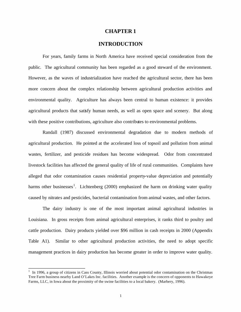
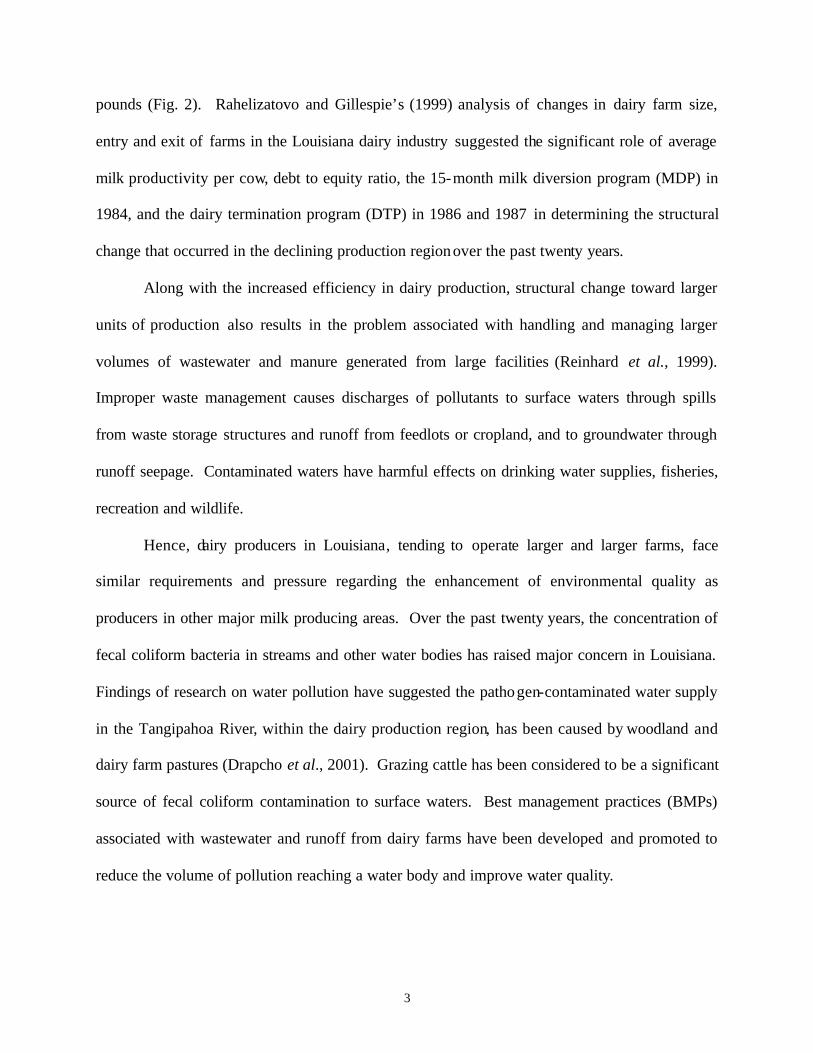
in the nation, toward fewer yet larger units of production. The declining trends in the number of
dairy farms, number of milk cows, total production of milk and gross farm income from dairy
products are shown in Figure 1.
The number of commercial dairy farms decreased from 995 in 1981 to 448 in 2000, a
drop of 55 percent. Over the twenty-year period, total milk production in Louisiana declined by
29 percent, from 996 million pounds in 1981 to 705 million pounds in 2000. Average milk
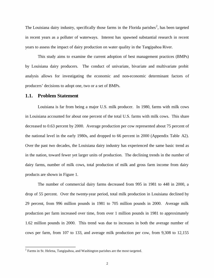
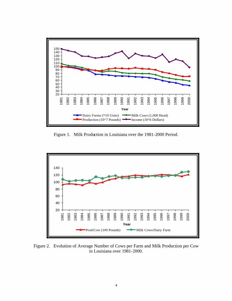
production per farm increased over time, from over 1 million pounds in 1981 to approximately
1.62 million pounds in 2000. This trend was due to increases in both the average number of
cows per farm, from 107 to 133, and average milk production per cow, from 9,308 to 12,155
2 Farms in St. Helena, Tangipahoa, and Washington parishes are the most targeted.
3
pounds (Fig. 2). Rahelizatovo and Gillespie’s (1999) analysis of changes in dairy farm size,
entry and exit of farms in the Louisiana dairy industry suggested the significant role of average
milk productivity per cow, debt to equity ratio, the 15-month milk diversion program (MDP) in
1984, and the dairy termination program (DTP) in 1986 and 1987 in determining the structural
change that occurred in the declining production region over the past twenty years.
Along with the increased efficiency in dairy production, structural change toward larger
units of production also results in the problem associated with handling and managing larger
volumes of wastewater and manure generated from large facilities (Reinhard et al., 1999).
Improper waste management causes discharges of pollutants to surface waters through spills
from waste storage structures and runoff from feedlots or cropland, and to groundwater through
runoff seepage. Contaminated waters have harmful effects on drinking water supplies, fisheries,
recreation and wildlife.
Hence, dairy producers in Louisiana, tending to operate larger and larger farms, face
similar requirements and pressure regarding the enhancement of environmental quality as
producers in other major milk producing areas. Over the past twenty years, the concentration of
fecal coliform bacteria in streams and other water bodies has raised major concern in Louisiana.
Findings of research on water pollution have suggested the pathogen-contaminated water supply
in the Tangipahoa River, within the dairy production region, has been caused by woodland and
dairy farm pastures (Drapcho et al., 2001). Grazing cattle has been considered to be a significant
source of fecal coliform contamination to surface waters. Best management practices (BMPs)
associated with wastewater and runoff from dairy farms have been developed and promoted to
reduce the volume of pollution reaching a water body and improve water quality.
4
2030405060708090
100110120130140150
1981
1982
1983
1984
1985
1986
1987
1988
1989
1990
1991
1992
1993
1994
1995
1996
1997
1998
1999
2000
Year
Dairy Farms (*10 Units) Milk Cows (1,000 Head)Production (10^7 Pounds) Income (10^6 Dollars)
Figure 1. Milk Production in Louisiana over the 1981-2000 Period.
20
40
60
80
100
120
140
1981
1982
1983
1984
1985
1986
1987
1988
1989
1990
1991
1992
1993
1994
1995
1996
1997
1998
1999
2000
Year
Prod/Cow (100 Pounds) Milk Cows/Dairy Farm
Figure 2. Evolution of Average Number of Cows per Farm and Milk Production per Cow in Louisiana over 1981-2000.
5
1.2. Justification
The agricultural community has traditionally been viewed as a good steward of the
environment. However, there has been increasing concern about the complex relationship
between farming activities and environmental quality. The significant role of agriculture as a
major source of several nonpoint source pollutants such as sediment, nutrients, pesticides, salt
and pathogens has been pointed out. Different studies have investigated the extent of BMP
adoption in crop production since the release of the U.S. Environmental Protection Agency
(EPA) guidance and specification of management measures for sources of nonpoint pollution in
coastal waters, in 1993 and revised in 1997. Findings of these studies have suggested a low level
of adoption of some BMPs and the need of more aggressive extension programs to convince crop
producers of the benefits of implementing specific BMPs for their land.
Agricultural production is not limited to crop production but embraces diverse activities.
A comprehensive understanding of the reduction of water pollution from agricultural nonpoint
sources would require similar investigation conducted in crop production to be applied to other
agricultural activities. Information on how other agricultural industries aim at reducing water
pollution is of importance. This study focuses on the voluntary implementation of BMPs in the
dairy industry. BMPs for Louisiana dairy farms target the reduction of soil, nutrients, pesticides
and microbial contaminants entering surface and groundwater while maintaining or improving
the productivity of agricultural land. The set of conservation practices comprises twenty one
specific practices. Dairy producers are encouraged to voluntarily implement these BMPs to
improve the quality of water in Louisiana. Knowledge of the current rates of adoption of BMPs
as well as the types of producers most likely to adopt will allow for the implementation of
extension and economic incentive programs to encourage further adoption.
6
1.3. Objectives of the Study
This study aims to assess the extent of current adoption of BMPs in the Louisiana dairy
industry and to determine the effect of demographic, socioeconomic and farm characteristics on
dairy farmer adoption of BMPs. It determines the type of producer that is most likely to adopt
specific conservation practices, enabling users of the research to target specific farm types for
programs to encourage the adoption of BMPs.
Specific objectives of the study include:
1. Determine the current efforts to contain water quality degradation, including regulatory
measures, research and educational programs on environmental issues as they relate to
Louisiana dairy production;
2. Review the literature on technology adoption in the agricultural sector;
3. Assess the extent of current adoption of BMPs in the Louisiana dairy industry;
4. Determine the effect of demographic, socioeconomic and farm characteristics on dairy
producers’ decisions to adopt specific BMPs; and
5. Make policy recommendations based on the empirical results.
A comprehensive review of literature on technology adoption in the agricultural sector
allow for the fulfillment of objective two. The extent of current adoption of BMPs in the
Louisiana dairy industry is assessed based on dairy producer responses obtained from a mail
survey conducted during Summer, 2001. Producers were asked to check any of the practices
they currently implement, and the possible reasons for not implementing the others.
Qualitative response econometric models are developed and analyzed to identify the
variables that significantly influence dairy producers’ decisions to implement or not implement a
specific management practice. Univariate, bivariate and multivariate probit analyses are
7
conducted. Univariate probit analysis focuses on current implementation of a single
management practice. Bivariate and multivariate probit analyses examine the adoption of a set
of two or more management practices simultaneously.
1.4. Background
1.4.1. Point and Nonpoint Sources of Pollution
Water pollution can result from two different sources. A point source is defined as “any
discernible, confined and discrete conveyance, including but not limited to any pipe, ditch,
channel, tunnel, conduit, well, discrete fissure, container, rolling stock, concentrated animal
feeding operation, or vessel or other floating craft from which pollutants are or may be
discharged. This term does not include agricultural storm water discharges and return flows from
irrigated agriculture” (Section 502 (14) of the Clean Water Act (CWA) of 1987). Point sources
of water pollution generally originate from identifiable sites and discharge sources. These
sources are subject to the permit requirements of the CWA.
A nonpoint source is technically defined as any other source of water pollution that does
not meet the legal definition of a point source (EPA, 2000). Water pollution that results from a
nonpoint source involves discharges not occurring at a single location. Nonpoint source
pollution takes place in a diffuse manner and is mostly related to meteorological events such as
rainfall and snow melt. Natural and manmade pollutants are carried over and through the ground
and reach surface waters such as lakes, rivers, streams, wetlands and other coastal waters as well
as ground water.
Studies conducted by the EPA have pointed out the gains in controlling point sources of
pollution, yet the water quality problem has not been solved. Since the late 1980s, there has been
a rising awareness of the significant influence of nonpoint sources of pollution that results from
8
human activities on land. A wide variety of means carries pollutants to surface water. The EPA
developed guidelines that specified different management measures for sources of nonpoint
pollution in coastal waters in 1993, and a revised version of the guidance in 1997. The
guidelines focused on appropriate source control measures and pollution delivery reduction in
five major categories of nonpoint sources pollution: agricultural runoff; urban runoff;
silviculture; marinas and recreational boating; and canalization and channel modification.
Management measures for agricultural sources aim at lessening pollution from erosion
and sediment, wastewater and runoff from confined animal facilities, and better management of
nutrient, pesticide, grazing, and irrigation on farm land. Management practices specific to the
source of pollution, location and climate can be applied to successfully control the addition of
pollutants to surface and coastal waters. Appropriate combinations of these practices, known as
best management practices (BMPs), are determined to be effective and practical means to reduce
water pollution from agricultural activities.
1.4.2. Water Quality Degradation
Water quality is defined according to the principal use of the resource. The CWA of 1972
describes water quality of designated beneficial uses such as drinking water supply, recreational,
and aquatic life support by means of numerical criteria that set physical, chemical and biological
norms, as well as narrative criteria that state the conditions required to be maintained for the
designated use. Reports on water quality assessment in the U.S. indicate a largely improved
surface water quality since the enactment of the CWA (EPA, 2000a; USDA-ERS, 2000). Such
achievement is mainly attributed to the technology and performance based regulatory approach to
reduce pollution from point sources. Assessment results also show continued discharges from
point sources and an increased contribution of discharges from nonpoint sources, implying the
9
need for a sustained effort to reduce water pollution. Reports on water quality across all water
bodies indicate that, in 1998, 35 percent of assessed river miles, 45 percent of assessed lake acres,
and 44 percent of estuary square miles are polluted (EPA, 2000a).
In Louisiana, the Tangipahoa River, within the dairy production region, has been subject
to environmental problems from nutrient and sediment pollution, bacterial contamination from
improperly functioning municipal wastewater treatment facilities, runoff and discharges from
dairies and concentrated animal operations, as well as truck farming and forest harvest areas
(EPA, 1995). The Louisiana Department of Environmental Quality (LDEQ) developed projects
within the Tangipahoa River watershed to deal with bacterial and nonpoint source pollution, and
promoted the implementation of NRCS designed lagoon systems by dairy producers in
Tangipahoa parish.
1.4.3. Agricultural Pollution
Studies have pointed out the significant role of agriculture as a major nonpoint source of
water pollution (EPA, 1998; Kahn, 1998; Knutson et al., 1998; Ribaudo et al., 1999). Pollutants
that originate from agriculture include sediment, nutrients (nitrogen and phosphorus), pesticides,
salts, and pathogens. Although agricultural activities are not the only source of nutrient
pollutant, nitrogen from animal waste constitutes an important source of total nitrogen loads in
some parts of the U.S. Similar to nutrients, pesticides move to water resources in run-off, run-in
and leaching. Furthermore, they can be carried into the air and deposited to water bodies with
rainfall. The possibility of pathogen-contaminated water supplies has attracted increasing
attention. The EPA reports released in 1998 indicate that bacteria constitute the second leading
cause in estuaries and the third leading impairment of rivers. Inadequa tely treated human waste,
wildlife, and animal operations are identified as potential sources of bacteria. Microorganisms in
10
livestock waste may cause several human diseases through direct contact with contaminated
water or consumption of contaminated drinking water and/or contaminated shellfish.
1.4.4. Environmental Policy in Agriculture
Improving environmental quality through sustainable agricultural production is not an
easy task. The questions of whether and how the government should intervene to correct
environmental externalities have been discussed by many. Policy debates have been conducted
and decisions made since Pigou’s arguments for government intervention in the late 1930’s and
Coase’s view of a market solution and negotiation process in the early 1960’s. Pigou (1938)
introduced the concept of externality taxes to eliminate the discrepancy between marginal private
cost and marginal social cost. Appropriate taxes against the offending party would allow for
internalizing the externality and achieving an efficient level of pollution emissions. Coase
(1960), on the other hand, perceived the use of a tax as unnecessary and argued for the
development of a market for the externality to achieve an optimal level of emissions, regardless
of the definition of property rights. Concerned groups would negotiate to achieve a mutually
profitable agreement, as long as the transaction cost is lower.
The presence and persistence of an environmental externality, however, can be attributed
to market failure and therefore prevents the conduct of the Coasian market approach. Researchers
have discussed different policy instruments for achieving environmental goals (Randall, 1987;
Weersink et al., 1997; Kahn, 1998). Governmental interventions to correct market failures
associated with environmental externalities include: moral suasion, direct production of
environmental quality, pollution prevention, command and control regulations and economic
incentives.
11
Moral suasion, which consists of persuading the public about the benefits of behaving in
a desired manner, has been used to influence individual behavior without specifying any rules. Its
extensive use in agro-environmental policy intends to encourage agricultural operators to enhance
environmental quality by adopting appropriate management practices. Yet, such voluntary
approaches may not be applicable in many situations and can have limited effectiveness with the
“free rider” problem. Individuals may consider their actions as minor in the collective effort. If
the individual views his or her contribution as worthless, this would lead to a suboptimal
provision of environmental quality in the long-run.
The second policy instrument consists of governmental programs that promote direct
production of environmental quality. This ameliorative approach would include actions such
as planting trees, stocking fish, creating wetlands and cleaning up toxic sites, and has been
successful at improving environmental quality. These first two policy instruments are both
appealing. However, the limited possibilities to use either have urged policy makers to develop
more rigorous courses of action. Pollution prevention programs aim at developing more
profitable and cleaner technologies. They promote the joint efforts of governmental agencies,
universities, and private firms to develop research programs to reduce pollution. The efforts aim
to address the lack of information associated with pollution production.
Command and control regulation is a direct control policy. It has been widely used to
modify harmful behavior toward the environment by directing polluters to comply with allowable
levels of pollution, and adopt the promoted type of activities or technologies to be used. Failure
to adhere to such restrictions would result in penalties. Direct control policy has generally been
under criticism because it may lead to greater abatement costs than necessary. Indeed, the
minimum abatement costs would be achieved only if the assigned pollution levels are based on
12
equal marginal abatement costs across polluters (Kahn, 1998, p. 62). Nevertheless, direct control
constitutes an appropriate policy instrument to face emergencies and reduce environmental
externalities that require high monitoring costs and/or very low optimal levels of pollution
emissions.
Incentive-based mechanisms, mostly economic incentives, are expected to alter
individual behavior and cause self- interest to agree with social interest. Individuals are given
incentives to voluntarily modify their actions toward more environmentally friendly behavior.
Economic instruments may include a variety of incentives such as a deposit-refund system,
charges or subsidies, marketable pollution permits or transferable discharge permits, a pollution
liability system, etc.
Usually, a single policy instrument does not suffice to reduce all existing environmental
problems, nor is it appropriate for all situations. The effectiveness of a policy instrument in
achieving environmental goals generally depends on its ability to minimize total costs of attaining
the desired environmental objectives. The design of an appropriate environmental policy to
reduce pollution from agricultural sources is challenging. The diffused nature of pollution
emissions associated with agricultural activities rends the mission more difficult.
Programs that provide economic incentives are likely to be more successful in motivating
producers. They are more flexible than command and control regulation, and allow for achieving
the environmental target level at lower cost. Producers are also motivated since the cost savings
form the implementation of new technology or practice accrue directly to the firm (Weersink et
al., 1997).
13
1.5. Current Programs for Controlling Agricultural Pollution
Different programs and actions have been undertaken to address agricultural point and
nonpoint sources of pollution at both Federal and State levels. The EPA is the Federal authority
in charge of developing policies and programs on water quality. Several environmental laws have
been enacted since the Federal Food, Drug and Cosmetic Act of 1938. The Federal Water
Pollution Control Act, initially approved in 1948, has been revised over the years.
The U.S. Department of Agriculture (USDA) has also provided assistance to state
agencies, local government and producers to reduce erosion and chemical use in agriculture and
to improve water quality since the 1930s. The Conservation Technical Program (CTP) offered
technical assistance on soil and water conservation as well as water quality practices to farmers.
At the state level, farmers are given incentives to adopt management practices to reduce
agricultural nonpoint source pollution. State implementation of regulations and liabilities
provisions constitutes a step to move beyond a voluntary approach.
Federal and state actions targeting the enhancement of national water quality have been
steady over the years. Current programs include the pursuit of existing long-term programs
initiated over more than half a century ago as well as recent programs established to address
specific problems.
1.5.1. Current EPA Programs
Current EPA programs targeting water quality enhancement relate to the CWA of 1977,
which constitutes the primary Federal Law to address both point and nonpoint source pollution,
the Coastal Zone Act Reauthorization Amendment (CZARA) of 1990 that requires specific
measures for agricultural nonpoint sources of pollution, and the Safe Drinking Water Act of 1974
14
that establishes standards for drinking-water quality and water treatment requirements for public
water systems.
The Nonpoint Source Management Program, established by Section 319 of the CWA,
amended in 1987, gives EPA the authority to provide grants, program guidance and technical
support for state projects promoting nonpoint source management plans and other programs.
Such grants reached over $537 million in 1998 (USDA-ERS, 2000). Section 320, related to the
National Estuary Program (NEP) and section 314, linked to the Clean Lakes Program, authorize
USEPA to provide grants and technical assistance to states and local government for developing
and implementing comprehensive conservation plans to protect and restore estuary resources and
publicly owned lakes, respectively.
The Comprehensive State Ground Water Protection Program (GSGWPP), established in
1991, coordinates federal, state and local government programs addressing ground water quality.
EPA also has leadership in the conduct of regional water quality programs such as: the Great
Lakes Program, established in 1978 to restore and protect the Great Lakes water quality; the
Chesapeake Bay Program directing the restoration of the bay since 1983 and involving the states
of Maryland, Pennsylvania, Virginia and the District of Columbia; the Gulf of Mexico Program
established in 1988 to protect the Gulf resources and involving the States of Florida, Alabama,
Mississippi, Louisiana, and Texas; and the Lake Champlain Basin Program established by the
Lake Champlain Special Designation Act of 1990 jointly administered by EPA, the States of
Vermont and New York, and the New England Interstate Water Pollution Control Commission.
The CZARA remains the federally mandated program requiring specific measures for
agricultural nonpoint source pollution. The program obligates each of the 29 States and territories
with USEPA approved coastal zone management programs to implement their plans starting in
15
year 2004. Annual costs of CZARA management measures are estimated to be less than $5,000
per farm (USDA-ERS, 2000).
The Wellhead Protection Program (WPP), authorized in 1986 by the Safe Drinking Water
Act (SDWA), provides EPA the authority to approve state well protection programs. Forty five
states had been granted EPA approved WPP programs by December 1998. Amendment of the
SDWA in 1996 requires water suppliers to inform customers about the levels of certain
contaminants and associated EPA standards.
1.5.2. Current USDA Conservation Programs
Conservation programs promoted by USDA are generally voluntary and provide technical,
educational and financial (cost-sharing and incentive payments) assistance, rental and easement
payments as well as other program benefits. In 1999, reports indicate USDA allocated $286
million for water quality and conservation activities (USDA-ERS, 2000).
The Environmental Quality Incentives Program (EQIP), initiated in the 1996 Federal
Agriculture Improvement and Reform Act (1996 Farm Act), jointly administrated by NRCS and
the Farm Service Agency (FSA), provides technical, educational and financial assistance to
eligible farmers and ranchers in complying with federal, state, and tribal environmental laws, and
encourages the implementation of conservation practices to enhance environmental quality. The
program supplies up to 75 percent cost share for the implementation of conservation practices
related to cropland, grazing lands and timberland such as management of grassed waterways,
filter strips, and manure facilities. Incentive payments can also be extended to eligible farmers
implementing practices such as nutrient management, manure management, pest management,
irrigation water management and wildlife habitat management. EQIP has been reauthorized in
the Farm Security and Rural Investment Act of 2002, known as the 2002 Farm Bill, with an
16
approved funding of $6.1 billion over six years, starting with $400 million in fiscal year 2002 and
increasing to $1.3 billion in fiscal year 2006 (NRCS, 2002). Changes have been made regarding
its implementation. These changes include EQIP payments being made the same year as the
contract approval, a one year minimum EQIP contract length, up to a 90 percent cost-share for
beginning farmers and ranchers, and increased total cost-share and incentive payments to
$450,000 per individual over the life of 2002 Farm Bill regardless of the number of farms or
contracts. Sixty percent of the funds for EQIP are targeted to livestock production. EQIP and
similar incentive programs are expected to significantly impact the adoption of environmental
practices by agricultural producers.
Other USDA conservation programs are associated with crop production and land
management. The Conservation Technical Assistance (CTA) program, authorized by the Soil
Conservation and Domestic Allotment Act of 1935 and administered by NRCS, helps land-users
in planning and implementing conservation systems to reduce erosion and improve soil and water
quality. CTA provides assistance to farmers in complying with the highly erodible land and
wetland provisions of the Food Security Act, as well as participant farmers in USDA cost-share
and conservation assistance programs.
The Conservation Compliance Provisions enacted in the Food Security Act of 1985
require producers who farm highly erodible land to implement a soil conservation plan to remain
eligible for commodity price and income support, crop insurance, and farm loan programs. The
Conservation Reserve Program (CRP), established in the same Act as a voluntary long-term
cropland retirement program, provides participants with annual per-acre rent and half the cost of
establishing permanent land cover for retiring highly erodible and environmentally sensitive
17
croplands for 10 to 15 years. The Conservation Reserve Enhancement Program (CREP) consists
of State-Federal partnership programs targeting partial field retirement.
The Buffer Initiative established in 1997 assists landowners in installing 2 million miles
of conservation buffers by 2002, and improves pollutants interception. The Wetlands Reserve
Program, authorized in 1990 as part of the Food, Agriculture, Conservation and Trade Act of
1990, provides easement payments and restoration cost-shares to landowners who permanently
return prior-converted or farmed wetlands to initial wetland conditions. The Small Watershed
Program authorized in 1954 provides technical and financial assistance to states, local
government, and other organizations that voluntarily plan and install watershed based projects on
private lands. The Wildlife Habitat Incentives Program, created by the 1996 Farm Act, provides
cost-sharing assistance to landowners for developing habitat for wildlife and endangered species.
1.5.3. Current Conservation Programs in Louisiana
The protection, conservation and restoration of the natural resources of Louisiana has
involved the Natural Resources and Conservation Service (NRCS) through 43 local soil and water
conservation districts, 7 resource conservation development areas, over 50,000 landowners, and
many partners and volunteers. The team work also targets the prevention of threats to public
health and the sustainability of viable agricultural enterprises. An overview of some
conservation programs conducted in Louisiana is presented in the following sections.
There has been evidence of increased interest and participation of agricultural producers
in the EQIP program (NRCS, 2002). The total Louisiana EQIP fund application level reached
$13,947,032 over the period 1997-2000 with over 4,848 contracts funded. The 660 new contracts
established in 2001 with funding of $3,188,669 involved cropland (51 percent), livestock
18
production (47 percent), and forestland (2 percent). The total number of contracts established
over the 1997-2002 period was 5,508 with a cumulative funding of over $17 million.
Louisiana has recorded 96 percent of the total Wetland Reserve Program (WRP)
easements in the nation, conferring the state the lead in acres enrolled in WRP in December 2000.
More than $94 million had been invested in the WRP in Louisiana by December 2000, to restore
87,102 acres in 24 parishes in the north and central parts of the state. By December 2001, the
total number of WRP easements recorded had increased to 374, involving 139,801 acres of land.
Over 13 thousand new acres were restored in 2001, yielding a total of 100,391 acres restored in
Louisiana.
The Louisiana Grazing Lands Conservation Initiative (GLCI) constitutes a part of the
voluntary nationwide effort to address owners and managers of grazing lands concern for
resource needs and technical assistance. Over 4 million acres of grazing lands have been
identified in Louisiana, including pastureland, rangeland, grazed woodlands, and potentially-
grazed cropland. During 2000, NRCS established 8 specific projects that involved 33 livestock
producers. The program aims at strengthening partnerships with the University of Louisiana at
Lafayette for the completion of a dairy grazing research project, and promotes voluntary action
through technical assistance for the application of NRCS prescribed grazing practices.
Agricultural producers are encouraged to diversify their farming activities to achieve multiple
benefits. The program provides training and education for NRCS employees as well as funding
assis tance to Research Conservation and Development councils for livestock educational tours.
Public awareness is enhanced through the organization of workshops, field days, livestock
producer meetings, and livestock publication.
19
A total of 2,654 contracts have been recorded in the Conservation Reserve Program (CRP)
in Louisiana. The program covers 207,235 acres of land in 41 parishes, and involves total annual
payments of $9,157,000 for restoring over 46,453 acres of cropped wetlands to approved
bottomland hardwood and native marsh cover.
Watershed projects have promoted the reduction and elimination of flooding problems,
improved water quality, and provided valuable irrigation water as well as economic development
on over 5 million acres of land in Louisiana. The Watershed Program has been administered by
NRCS under Public Law 83-566 since 1954. Major accomplishments have included the
completion of 37 projects (9 currently active), 4 recreational areas, 11 cooperative river basin
studies and the construction of dams, stabilization structures and channels with pipe drops. The
USDA Emergency Watershed Protection Program provides vital natural disaster relief assistance
after tropical storms, hurricanes and tornadoes. In 2001, NRCS completed emergency watershed
work for damage caused by tornadoes in Webster parish, and damage caused by tropical storm
Allison in East Baton Rouge parish.
Other conservation programs include the Wildlife Habitat Incentive Program (WHIP),
created in the 1996 Farm Bill to provide technical assistance and cost-share payments to
participants by voluntarily improving wildlife habitat on private land; the Forestry Incentives
Program (FIP), authorized by the Congress to provide cost-sharing assistance for tree planting,
timber stand improvement, and other related practices on non- industrialized, private forest lands;
and the Coastal Wetlands Planning, Protection, and Restoration Act (CWPPRA), known as the
Breaux Act of 1990 and reauthorized for nine more years in 2000 to carry out high priority
projects to protect and restore coastal wetlands.
20
1.6. Best Management Practices (BMPs)
1.6.1. Generalities
Best management practices consist of a specific set of practices determined to be effective
and practical means to prevent or reduce pollution from nonpoint sources associated with
agricultural activities, forestry, urban run-off, marinas, recreational boating and channel
modification. Management practices are site specific. Indeed, BMPs are usually designed to
control a particular pollutant type from specific land uses by minimizing the delivery and
transport of pollutants available to surface and ground waters.
Implementation of BMPs is generally voluntary. However, such implementation may
move toward a regulatory means of nonpoint pollution control, provided that the specified
management measures are economically feasible. As Knutson et al. (1998) emphasized,
economic incentives including conservation compliance, green payment, or regulation could
improve the implementation of BMPs.
General measures for containing agricultural nonpoint sources of pollution include:
control of erosion and sediment ; management of wastewater and runoff from confined animal
facilities3 (large or small units); effective use of nutrients and pesticides; protecting range, pasture
and other grazing lands; and managing irrigation water. A confined animal facility is described in
the EPA guidance of management measures as “a facility where animals are stabled or
maintained for a total of 45 days or more within any 12-month period and crops, vegetation
forage growth, or post-harvest residues are not sustained in the normal growing season over any
portion of the lot or facility” (EPA, 1993).
3 Management measures are relevant to all new facilities regardless of their size. They are also appropriate to existing animal facilities. Dairies with at least 70 animals, equivalent to 98 animal units, are considered as large facilities, and operations with 20 to 69 animals, corresponding to 28-97 animal units, are classified as small farms. (EPA, 1997).
21
The animal feeding operation (AFO) strategy, released in 1999, emphasizes the use of
regulatory and voluntary incentive-based approaches to minimize water quality and public health
impacts from improperly managed animal manure and wastewater, while preserving and
enhancing sustainability of livestock production. AFO operators are expected to take actions to
reduce water pollution by developing and implementing site-specif`ic comprehensive nutrient
management plans (CNMPs). These plans include conservation practices and management
activities that promote the use of manure and organic by-products as beneficial resources and
lessen the adverse impacts of AFOs on water quality.
Given the controversial issues associated with concentrated animal feeding operations
(CAFO)4, specific guidance was developed in 1999 to provide information on permitting
requirements for CAFOs. The CAFO designation concerns operations that confine a large
number of animals and store wastewater and manure in a contained area for extended periods of
time.
The AFO strategy described the two-phase approach to issue National Pollutant
Discharge Elimination System (NPDES) permits to CAFOs. During the first phase from 2000 to
2005, EPA and State permitting authorities refer to existing NPDES regulations to ensure CAFO
compliance with applicable water quality standards. The second phase, beginning in 2005, will
consist of reissuing NPDES permits to CAFOs based on revised effluent limitation guidelines for
feedlots and NPDES regulations.
1.6.2. Best Management Practices for the Louisiana Dairy Industry
A team effort led by the Louisiana State University Agricultural Center developed BMP
manuals aimed at reducing the impact of agriculture on Louisiana’ s environment. BMPs for
22
Louisiana dairy farms target the reduction of soil, nutrients, pesticides and microbial
contaminants entering surface and groundwater while maintaining or improving the productivity
of agricultural land (LSU Agricultural Center, 2000).
Management practices targeting the reduced impacts of agriculture on Louisiana’s
environment include twenty one specific practices. They refer to specific NRCS codes and are
implemented on agricultural land for different purposes. The description presented below was
borrowed from the EPA specification of management measures and the BMP manual for dairy
production in Louisiana.
Conservation tillage (NRCS Code 329) is described as a system designed to manage the
amount, orientation and distribution of crop and other plant residues on the soil surface year-
round. Crop residues are maintained at or near soil surfaces. Such a management system
improves water flow into and through the root zone, reduces soil erosion and sediment transport
by providing soil cover during critical times in the cropping cycle and influences the movement
of nitrogen from the soil-plant system into the environment. Nitrogen losses associated with soil
erosion and surface runoff are greatly reduced.
Cover and green manure crop (NRCS Code 340) consists of establishing a crop of
close-growing grasses, legumes or small grains for seasonal protection and soil improvement.
The crop is usually grown for one year or less except where there is permanent cover. This
practice is designed to control erosion during periods when major crops fail to furnish enough
cover. Winter cover can absorb nitrates and available water for the remaining season and
therefore reduce the potential of nitrogen to leach. The cover crop, once returned to the soil,
4 An animal feeding operation is designated as a CAFO by the permitting authority on a case-by-case basis. CAFOs generally confine more than 1,000 animal units at the facility. The definition extends to smaller operations with 300 to 999 animal units, discharging pollutants directly into waters of the U.S.(EPA, 2000b).
23
provides organic materials that improve soil structure with better infiltration capacity, aeration
and tilth.
Critical area planting (NRCS Code 342) involves the planting of vegetation such as
trees, shrubs, vines, grasses, or legumes on highly erodible or critically eroding areas, excluding
planting trees for wood products. This practice aims at reducing soil erosion and sediment
delivery to downstream areas and at improving wildlife habitat and aesthetics. Plants may also
take up more of the nutrients in the soil, reducing the amount of nutrients washed into surface
waters or leached into ground water.
Field borders (NRCS Code 386) consist of strips of perennial vegetation established at
the edge of a field to reduce erosion. Field borders serve as anchoring points for contour rows,
terraces, diversions and contour strip cropping. The use of a field border may reduce the quantity
of sediment and related pollutants delivered to surface waters. Other purposes include erosion
control, protection of edges of fields used as turn rows or travel lanes for farming machinery,
reduced competition from adjacent woodland, food and cover provisions for wildlife, and
landscape improvement.
Filter strips (NRCS Code 393) are vegetative areas designed to trap sediment, organic
material, nutrients and chemicals from runoff and wastewater, and thus reduce pollution and
protect the environment. Implementation of filter strips relieves the problem associated with
fertilizer and herbicide application close to susceptible water sources. In general, filter strip
effectiveness depends on the quantity of sediment reaching the strip, the amount of time the water
is retained, the infiltration rate of the soil, the uniformity of water flow through the filter strip, and
the quality of maintenance.

24
Grassed waterways (NRCS Code 412) consist of natural or constructed channels shaped
or graded to required dimensions. They are established with suitable vegetation to stabilize the
conveyance of runoff from terraces, diversion or other water concentration. The design of the
channel aims at reducing erosion in concentrated flow areas as well as improving water quality by
filtering out suspended sediment.
Heavy use area protection (NRCS Code 561) stabilizes areas frequently and intens ively
used by people, animals or vehicles by establishing vegetative cover, surfacing with suitable
materials, or installing needed structures. Design criteria include drainage and erosion control,
appropriate structures according to engineering standards and specifications, and suitable
vegetation to reduce erosion as well as air and water pollution.
Regulating water in drainage systems (NRCS Code 554) directs the operation of water
control structures. This management practice is designed to regulate the outflow from drainage
systems and thereby remove surface runoff. It aims at conserving surface or subsurface water and
maintaining soil moisture conditions, specifically in organic soil and in highly permeable soil of
low water capacity. The outflow controls should be designed based on the amount of water
available and the degree of water control required.
Riparian forest buffers (NRCS Code 391) are areas of trees, shrubs or other vegetation
adjacent to and uphill from water bodies. Buffer zones can be established on cropland, hay land,
rangeland, forestland or pastureland neighboring permanent streams, lakes, rivers, ponds,
wetlands, and other water bodies with high potential of water quality impairment. They create
shade to lower water temperature and improve habitat for aquatic organisms, provide habitat and
corridors for wildlife, and remove excess amounts of sediment, organic material, nutrients,
pesticides and others pollutants in surface water.
25
A sediment basin (NRCS Code 350) is constructed for manure, waterborne sediment
and debris storage purposes. Its design assists in maintaining the capacity of lagoons, preventing
bedding materials from entering waste disposal systems, and preventing manure from moving to
fields. Sediment basin capacity should be based on the expected volume of sediment to be
trapped at the site.
Streambank and shoreline protection (NRCS Code 580) uses vegetation or structures
to stabilize and protect banks of streams, lakes, estuaries, or excavated channels against scour and
erosion. This practice applies to natural and excavated channels threatened by water erosion,
livestock damage and vehicular traffic.
Roof runoff management (NRCS Code 558) deals with the collection, control and
disposal of runoff water from roofs. The practice is designed to reduce erosion and pollution by
preventing roof runoff water from flowing across concentrated waste areas, barnyards, roads and
alleys. It is also applied for drainage improvement and environmental protection.
A waste management system (NRCS Code 312) is a planned system installed for
managing liquid and solid waste, including runoff from concentrated waste areas. This practice is
designed to preclude or minimize degradation of air, soil, and water resources, and to protect
public health and safety. The system may consist of a single component or several components
such as waste storage ponds, waste storage structures, waste treatment lagoons, waste utilization.
A waste storage facility (NRCS Code 313) consists of a waste impoundment made by
constructing an embankment and/or excavating a pit, or a structure. The construction is designed
for temporary storage of wastes such as manure, wastewater and contaminated runoff. The
standard establishes the minimum acceptable requirements for planning, designing, constructing,

26
and operating waste storage facilities including waste storage tanks, waste stacking facilities and
settling basins, but excluding waste treatment lagoons.
A waste treatment lagoon (NRCS Code 359) is a waste impoundment made by
excavation or earthfill for temporarily storing and biologically treating organic wastes from
animal and other agricultural activities. Standards for waste treatment lagoons differ from those
for waste storage ponds and waste storage structures. Lagoons must be located near the source of
the waste, far from neighboring dwellings (a minimum distance of 300ft) and water wells (a
minimum distance of 150 ft), and where prevailing winds carry odors away from residences and
public areas.
Waste utilization (NRCS Code 633) involves the use of wastes from agricultural and
other activities on land in an environmentally acceptable manner. This practice aims at
maintaining and/or improving soil and plant resources. Wastes are safely applied on land and
vegetation suited to the use of waste as fertilizer. Implementation of this practice is expected to
enhance crop, forage and fiber production, improve or maintain soil structure, prevent erosion and
protect water resources.
Nutrient management (NRCS Code 590) addresses the need for managing the amount,
form, placement and timing of the application of plant nutrients associated with organic waste,
commercial fertilizer, legume crops and crop residue. Comprehensive nutrient management plans
are developed to realize optimum forage and crop yields, minimize nutrient entry to sur face and
groundwater, and maintain and/or improve the soil chemical and biological conditions. Planning
considerations include a thorough evaluation of soil nutrient needs, an inventory of nutrient
supply, an assessment of nutrient balance, and monitoring procedures.

27
Pest management (NRCS Code 595) concerns the management of agricultural pest
infestations including weeds, insects and diseases, coherent with crop production and
environmental standards. The development of a pest management program promotes appropriate
cultural, biological, and chemical controls and includes planning considerations such as pest
management procedures, pesticide selection and application, and storage and safety measures.
Agricultural producers are urged to follow extension recommendations to ensure proper usage of
pesticides.
Fencing (NRCS Code 382) can be used as part of a conservation management system to
address soil, water, air, plant, animal and human resource issues. A constructed barrier is built to
control and/or exclude livestock or wildlife and regulate human access. Plans for fencing along
waterways should include crossings over waterways and provisions for animal drinking water
sources.
Prescribed grazing (NRCS Code 528-A) is applied as part of a conservation
management system to improve and maintain controlled harvest of vegetation for grazing
animals, and enhance the quality and quantity of water and soil conditions in the area. The
establishment of a prescribed grazing plan should include considerations of the duration,
intensity, frequency, and season of grazing to enhance nutrient cycling and minimize soil
compaction, and the needs of other enterprises such as wildlife and recreational uses.
A trough or tank (NRCS Code 614) provides livestock watering facilities at a selected
location that will protect vegetative cover. Watering facilities are supplied by streams, springs,
wells, ponds and other sources. This practice permits a desired level of grassland management,
reduces health hazards for livestock and prevents livestock waste in streams.
28
1.7. Dissertation Outline
The dissertation is organized into five chapters. The second chapter consists of a review
of relevant literature to the research problem. The third chapter focuses on data collection, the
theoretical framework and research methodology. Discussion about the implementation of the
mail survey, the conduct of principal component analysis to reduce the number of explanatory
variables in the bivariate and multivariate probit analysis, and the different tests included in the
study are provided. Descriptive statistics from the survey on Louisiana dairy producers along
with the empirical results of the analyses are presented in the fourth chapter. The last chapter
provides a summary and the conclusions of the study as well as some suggestions for further
research.
29
CHAPTER 2
LITERATURE REVIEW
This chapter consists of three major sections. Section one concentrates on selected
literature related to technological adoption in the agricultural sector. Section two presents a
review of selected empirical studies on conservation adoption over the past two decades. The last
section focuses on environmental attitude.
2.1. Technology Adoption in the Agricultural Sector
One of the earliest studies on technology adoption was Griliches’ exploration in 1957 of
the economics of technological change, specifically the wide differences in the rate of use of
hybrid seed corn. His interests led to investigation of the possibility that one can perform an
economic analysis on the process of innovation, and the adoption of a particular invention. He
emphasized the differences between the lag in “availability” due to the time- lag in the
development of adaptable hybrids for specific regions, and the lag in “acceptance” perceived in
the different rates of adoption by farmers, although both can be explained on the basis of varying
profitability of entry. He estimated the rate of acceptance along with other parameters for each of
31 states and 132 crop-reporting districts within these states. A logistic growth curve was
assumed, based on the graphical analysis of the state data on percentage of hybrid corn planted
over time. An S-shaped trend was found.
Average corn acres per farm, average difference between hybrid and open pollinated
yields and pre-hybrid average yield were included in linear and log regression estimations to
explain the farmer’s rate of acceptance. Results showed the substantial influence of the
differences in profitability from shifting to hybrids on adoption. Since the publication of
Griliches’ work, the economics of technology adoption has captured researchers’ interests,
30
yielding hundreds of publications. Selected literature of relevance to the present study is
presented in the following sections.
Feder et al. (1985) reviewed theoretical developments and empirical studies on adoption
of agricultural innovations in developing countries. The survey showed the dependency of
observed diffusion patterns on complex relationships between factors such as risks associated
with the new technologies, farmers’ attitudes toward risk, fixed adoption costs and cash
availability. The authors discussed the variables often hypothesized by a number of empirical
studies to influence farmers’ adoption decisions. These variables account for farm size, risk and
uncertainty, human capital, labor availability, credit constraints, supply constraints, and
landownership and rental arrangements. Feder et al. pointed out the tendency of empirical studies
to consider innovation adoption in dichotomous terms, and the need for appropriate econometric
tools to allow for the simultaneous nature of adoption decisions when farmers are presented a set
of new practices with various degrees of complementarity.
Caswell and Zilberman (1985) examined the determinant factors in the adoption of
furrow, sprinkler, and drip irrigation by fruit growers in the San Joaquin Valley of California.
Land shares of each technology type and for each region were included as estimates of adoption
probabilities in a multinomial logit model. Reliability of the results was assessed based on four
measures: the value of the log- likelihood function, McFadden and Efron R2 estimators, and the
percentage of correct predictions. This study emphasized the significant role of economic
considerations in determining farmers’ adoption of new irrigation technologies in California, and
the substantial water saving from water-price policies. An increase in a water tax would
encourage fruit growers to adopt modern technologies associated with water cost-saving. Such a
decision would lead to a decrease in water use.
31
Shields et al. (1993) performed a longitudinal analysis of factors influencing increased
technology adoption in Swaziland maize production. Their study provided insight into the
adoption process shaped by different factors and endowments such as farm size, farm labor, input
and output prices, capital availability, education, risk and uncertainty, and draft animal
ownership. Recommended farming practices included improved seed varieties, tractor plowing,
chemical fertilizers, and insecticides. A logistic model was applied to examine the probability
that a maize farmer would increase application rates of a selected technology over time. The
analysis was based on data collected from three surveys (in 1985, 1988, and 1991) of 85
households. Results showed the significant influence of four factors on maize farmers’ decisions
to adopt new technology: farmers’ ability to mobilize sufficient labor, the availability of capital,
farm size and risk aversion. The lack of cash would reduce the use of hybrid seed, basal and top
dressed fertilizer. Certainty in the expected rainfall, associated with higher anticipated output
levels would encourage farmers to adopt new technology.
Ghosh et al. (1994) investigated the effects of technical efficiency and risk attitudes on
the adoption of artificial insemination (AI) and/or computerized dairy herd inventory accounting
(DHIA) technologies in the U.S. dairy industry. The study was based on a two-step process.
First, individual firms’ technical inefficiencies were estimated using the stochastic production
frontier approach. Then, multinomial logit analysis was used to model technology choice.
Firms’ technical inefficiencies and producers’ risk attitudes were included as explanatory
variables in the logit analysis. The theoretical model assumed farmers’ knowledge of input and
output prices and acknowledged the risky aspect of technology adoption. Given the stochastic
nature of agricultural output, farmers would maximize expected utility, and would consider both
expected profit and variance of profit. Farmer’s risk attitude was assessed through participation
32
in government-program crops, off- farm income and insurance purchase on dairy assets. All
three variables were expected to have a negative sign in the multinomial logit model. The
findings of the study based on 145 cross-sectional data from the Appalachian dairy region
suggested significant effects of technical efficiency, milk prices and farmer’s risk aversion
behavior in the simultaneous adoption of both technologies.
Zepeda (1994) examined simultaneity of technology adoption and productivity in her
assessment of the determinants of DHIA technology adoption by California dairy farmers. She
emphasized the need for consistent and asymptotically more efficient generalized probit results
that would account for the joint determination of productivity and technology choice and avoid
biased estimates obtained from a single-equation. She considered a simultaneous system of
structural form equations, as well as generalized probit ordinary least squares and generalized
probit generalized least squares estimations to analyze 153 observations obtained from a
telephone survey of randomly selected California Grade-A milk producers. The findings of the
study suggested the need to correct for simultaneous equation bias in the investigation of
technology adoption. Single-equation estimates would lead to overstated significance of the
relationships as well as different conclusions concerning the factors affecting the decision to
adopt. The model, however, suffered from a high degree of multicollinearity, affecting the
significance of the coefficients.
Dorfman (1996) modeled the multiple adoption decisions of U.S. apple growers over two
technologies in a joint framework, given the fact that it is essential to understand multivariate
adoption decisions. Apple growers’ adoption decisions on integrated pest management practices
(IPM) and improved irrigation techniques were examined using four technology-bundle choices:
neither technology; integrated pest management only; improved irrigation only; and both
33
technologies. Analysis based on the four possible related choices was expected to provide a
better understanding of the characteristics associated with techno logy adoption and an improved
forecast ability. Farmers’ decisions to adopt were analyzed using a univariate probit model for
each technology and a multinomial probit model to account for the interrelationships among
decisions. A Bayesian approach using Gibbs sampling was developed to address the
computational problem associated with the maximum likelihood estimation of the n-dimensional
cone integrals in the multivariate normal distribution. Findings of the study suggested a 60.3%
accuracy rate of prediction (adoption decision correctly predicted). Results showed the
importance of education level and the amount of off- farm work on the farmer’s decision to
adopt. A strong negative covariance was found between adoption of IPM and improved
irrigation, challenging the tendency to believe that farmers who adopt advanced technologies
necessarily tend to adopt many of them. The study suggested that IPM practices and improved
irrigation techniques were not adopted simultaneously by the same farmers.
El-Osta and Morehart (1999) investigated the effects of herd expansion and other factors
on dairy farmer decisions to adopt a capital- intensive and/or a management- intensive technology.
Based on national data from the 1993 USDA Farm Costs and Returns Survey, the authors
estimated a multinomial logit model to illustrate the economics of choosing among four types of
technologies: a capital- intensive technology (an array of advanced milking parlors); a
management- intensive technology (the Dairy Herd Improvement production record keeping
system); a combined adoption of both technologies; and the choice of neither. Findings of the
study suggested a significant role of educational attainment, farm operator’s age, ownership of
land and farm size in the choice and adoption of technology. Alternative simulations were run
using the estimated coefficients and different farm sizes in order to assess the effects of farm
34
expansion (doubling or tripling farm size) on the likelihood to adopt a technology. The pattern
of adoption was found to be sensitive to herd expansion, which supports the idea of scale-
biasedness in technology adoption. The authors concluded that benefits from farm expansion
and technology adoption would remain possible providing that the purpose would be to lower
per-unit costs through enhanced production efficiency rather than sole ly increasing per-cow
yields.
Reinhard et al. (1999) analyzed the technical and environmental efficiency of Dutch
dairy farms. The study was based on production activities of 613 strongly specialized dairy
farms in the Dutch Farm Accountancy Data Network over the 1991-1994 period. The authors
estimated a stochastic translog production frontier using a single index of dairy farm output, and
three categories of aggregate inputs including LABOR, CAPITAL, and variable INPUT.
Nitrogen surplus from application of excessive amounts of manure and chemical fertilizer was
also included as an environmentally detrimental input. The derived output-oriented measure of
technical efficiency was computed as the ratio of observed level of output to maximum feasible
output. The authors estimated the environmental efficiency associated with each farm using the
“+ V formula” based on the assumption that a technically efficient farm is necessarily
environmentally efficient. Findings of the study emphasized the generally high levels of
technical efficiency (89 to 90 percent on average) and the low levels of environmental efficiency
(44 percent on average although steadily increasing over the sample period) achieved by the
Dutch dairy farms. The estimated shadow prices of nitrogen surplus of 3.1 1991 guilders per
kilogram of nitrogen surplus could provide the Dutch government information on appropriate
taxes on nitrogen surpluses. Results also emphasized the weak positive relationship between
environmental efficiency and intensity of dairy farming.
35
Davis and Gillespie (2000) examined technology adoption in U.S. hog production. Their
focus was to determine the impact of financial, demographic, and struc tural variables on the
adoption of four breeding practices and five production management practices in the hog
industry. The effects of twenty-two identified explanatory variables on the decision to adopt
specific technologies were assessed using a binomial logit analysis and 1025 observations
obtained from a national mail survey. The influence of financial and socioeconomic aspects on
the biosecurity of the operation was also examined using a two-limit tobit model. The findings
of the study, consistent with the results in previous publications, supported the notion of scale-
biasedness in favor of larger firms in the adoption of most of the technologies and managerial
practices considered in the analysis.
Moser and Barrett (2002) investigated the complex dynamics of smallholder technology
adoption of rice producers in Madagascar. They examined the potential determinants in the
farmer’s decision to adopt a high yielding and low external input technology known as system of
rice intensification. They proposed a framework that took into account the importance of time
and experience in learning a new method, the critical constraints on family labor and seasonal
liquidity, as well as the possibility of nonmaterial preferences. Results of the study based on
quasi-panel data and recall data related to 317 households in five villages emphasized the key
roles of learning effects, financial constraints and labor availability in farmers’ decisions to
experiment with and adopt a new technology.
2.2. Empirical Studies on Conservation Technologies
Conservation technologies or practices considered in this section include
environmentally-sound technologies, which differ from other technologies implemented in the
production process. Selected literature is presented.
36
Gould et al. (1989) investigated the role of farm and operator characteristics in
conjunction with the perception of soil erosion in understanding the adoption and use of
alternative tillage practices by Wisconsin farmers. The ir analysis, based on the 1987 Wisconsin
Family Farm Survey (WFFS), involved two stages. The first stage examined the producer’s
level of awareness of soil erosion. The binary dependent variable, PERCEIVE, was set to one if
the farm operator strongly agreed that soil erosion was an important problem in the area, and
zero otherwise. The second stage analyzed farmers’ adoption of conservation practices. The
farmer’s perception of soil erosion was derived from the probit analysis in the first stage. Then,
predicted perception was included as a determinant of the farmer’ s adoption decision in the two-
limit tobit analysis in the second stage. Findings of the study emphasized the importance of land
slope steepness and contact with the Soil Conservation Service on farm operators’ awareness of
soil erosion problems in their area. Results also suggested that younger farmers operating larger
farms were more likely to adopt soil conserving technologies, and reliable information gathering
and dissemination systems could improve the effectiveness of voluntary adoption programs.
Barbier (1990) analyzed the farm-level economics of soil conservation in the uplands of
Java, Indonesia, and concentrated on farmers’ decisions to invest in the control of soil loss and
land degradation. The upland conservation technical packages include construction of bench
terraces in areas of up to 50 percent slopes in conjunction with improved cropping patterns, and
agro-forestry-based systems on areas with greater slopes. Results of the study suggested that the
farmer’s decision to adopt a soil conservation strategy was influenced by the correlation between
land erodibility and profitability of different farming systems on different soils and slopes.
Furthermore, appropriate economic incentives would likely provide farmers with motivation to
adjust their land management practices and farming systems.
37
Govindasamy and Cochran (1995) used an integrated approach to analyze the economics
of the conservation compliance program and adoption of five best management practices in
Iowa. The management practices included fall plow, spring plow, and conservation tillage with
20 percent, 30 percent, and 40 percent crop residues. The authors developed a linear
programming model to analyze three scenarios related to a typical 350-acre Iowa farm and 12
selected soil types and percent slopes: Marshal (5 to 10 percent); Monoma (5 to 10 percent);
Kenyon (2 to 5 percent); Kenyon (5 to 10 percent); Tama (2 to 5 percent); Clarion (2 to 5
percent); Clarion (55 to 10 percent); Downs (5 to 10 percent); Fayette (5 to 10 percent); Otley (2
to 5 percent); Galva (5 to 10 percent); and Sharpburg (2 to 5 percent). Marginal values of
different soil types were obtained from the efficiency analysis of the Conservation Compliance
Program (CCP). Govindasamy and Cochran suggested that society could benefit from farmers
greater compliance to the program if marginal values of soil were equal across different types of
soil. A higher net return from compliance also would enhance farmers’ motivation to adopt
management practices.
Lynne (1995) attempted to modify the neo-classical approach to technology adoption
with behavioral science models in his examination of water conserving technology adoption
behavior of Florida strawberry growers. He suggested the need for a multiple-utility framework
similar to the one in the theory of planned behavior model. In this model, behavior or intention
to act was determined by three components: the “I-utility” that reflects the producer’s self-
interest; the “We-utility” that accounts for the commitment, meta-preferences or moral
dimensions; and the perceived behavioral control reflected in capital constraints and the
producer’s profit maximizing behavior. Tobit regression analysis was performed based on data
obtained through personal interview of 44 strawberry growers. Three different scenarios were
38
estimated depending on the type of utility considered: the mono-utility model (producers’ utility
uniquely from profit maximization); the profit seeking and I-utility model; and all three types of
utility. Results of the study suggested that behavior in conservation technology adoption would
be more than a strictly profit driven phenomenon.
Krause and Black (1995) evaluated the joint effects of machinery replacement decisions,
learning curves and risk aversion on optimal adoption strategies for no-till technology1 in
Michigan, using two normative dynamic analyses. Optimal machinery selection and acquisition
strategies for a representative expected profit-maximizing farmer, and a representative risk-
averse, expected utility-maximizing farmer were analyzed through separate dynamic
programming models. A deterministic model with maximization of time-discounted net revenues
was used for the first type of farmer. A stochastic model with maximization of a time-discounted,
semi- log expected utility function of net income was estimated for the second type of farmer.
Key parameters assumed in determining adoption strategies included crop yields, crop prices,
input costs, tractor and planter costs, tractor and planter residual values, and the discount rate.
The Markovian probabilities of price were included as additional parameters for the stochastic
model. Findings of the study emphasized the effects of planter age, current tractor age, relative
yield expectations, risk aversion, crop price expectations, the learning curve, and the discount rate
on the optimal time to adopt no-till technology. Results suggested that adjustment costs and risk
aversion could substantially delay adoption. Learning curve effects and risk aversion would
prevent adoption of no-till technology in the case of unfavorable crop price expectations.
Westra and Olson (1997) investigated the adoption of conservation tillage practices by
farmers in two count ies in East-Central Minnesota, and emphasized the importance of factors
1 No-till technology has been promoted for reducing soil erosion and production costs (Krause and Black, 1995).
39
such as information availability, consistency and relevance especially to local area, and the
existence of a support system or resources in the farmer’s decision process. Better quality of
information would enhance producers’ willingness to adopt conservation tillage practices whereas
the degree of support resources available would affect their ability to implement the practice. The
effects of hypothesized determinants of producers’ adoption decisions were estimated using five
logistic models: a base model that included the complete set of 25 explanatory variables and four
parsimonious models derived from the base model. The overall findings of the study are
consistent with previous research conclusions. Operators of large-sized farms, more concerned
about soil erosion issues on their land, engaged in a recent major farm investment, or primarily
informed about the practice by other farmers were more likely to adopt conservation tillage
practices. In this study, farmers’ experience was not found to be a significant factor in the
adoption decision.
Cardona (1999) assessed the feasibility of alternative approaches to meeting agricultural
nonpoint pollution control standards for sugarcane in Louisiana’s coastal zone management
areas. The study hinges on the neoclassical analysis of behavior which emphasizes individual
preferences, rational economic behavior and utility maximization as well as the analysis of
producers’ attitudes. Sugarcane producers’ adoption of best management practices (BMPs) was
hypothesized as being determined by different economic, socioeconomic, institutional and
attitudinal variables. Univariate probit and multivariate probit estimations to account for the
contemporaneous disturbances between the adoption of specific management practices were
analyzed based on 223 observations obtained from a mail survey of Louisiana sugarcane
producers in 1999. The findings of the study suggested a significant influence of number of
times producers met with extension service personnel, number of grower-meetings attended,
40
participation in cost-sharing, farmers’ beliefs of agricultural activities reducing the quality of
water coming off farmland, level of debt, and land tenure.
Soule et al. (2000) explored the relationship between tenure and adoption of conservation
practices. Logit regression models for conservation tillage and medium-term practices2 were
estimated, based on data from the 1996 Agricultural Resource Management Study survey
administrated by NASS and the NCRS-Oregon State University PRISM project. Farmers were
assumed to maximize private returns (present value of current net returns and terminal land
value). The base model included farmer attributes, attributes of the farm, variables specific to
the field, regional attributes and a dummy variable for tenure. Two dummy variables for cash-
rented and share-rented arrangements substituted for tenure variable in a modified model.
Findings of the study suggested that land tenure, timing of benefits, and land erodibility were
influential factors in a farmer’s decision to adopt conservation practices. Although all tenure
types adopted medium-term practices, cash-rent farmers were more likely to adopt conservation
tillage.
Ipe et al. (2001) simulated a Group Incentive Program to encourage farmer adoption of
BMPs for the Lake Decatur watershed in Central Illinois. The program promoted farmers’
participation in changing the timing of fertilizer application and reducing the application rate.
Financial incentives were considered as necessary to ease farmers’ skepticism about the
profitability of implementing these practices and to promote adoption. The model was based on
long-run group average profits received by both participating and non-participating farmers. An
incentive payment scheme was proposed to compensate farmers participating in the program for
2 Medium-term conservation practices included contour farming, strip-cropping, and grassed waterways. Adoption of any of these practices would require several years to generate positive benefits, while cost savings from conservation tillage would increase profits in the short-term.
41
eventual losses in profits, so as to receive at least the same level of profits as non-participating
farmers. Four alternative scenarios3 were simulated. Results of the study supported a lower
expected total profit for non-participants in all alternative reductions in nitrogen application.
Moreover, participants in the simulated program would achieve higher expected profits even
without an incentive payment. This would suggest a risk-averse farmer might be better off by
participating in the Group Incentive program, because current application of nitrogen fertilizers
could already be at rates above profit-maximizing levels. Thus, the proposed program would
increase farmers’ profits, reduce the variance of farmers’ profits, and mitigate nitrate pollution in
Lake Decatur.
Soule (2001) investigated the hypothesis that small farmers are better stewards of land
than larger farmers in her analysis of the adoption of six nitrogen management practices and five
soil management practices by U.S. corn producers in the 16 major corn producing states.4
Nutrient management practices would lower the cost of fertilizer applications and reduce nitrate
leaching and denitrification. Soil management practices, on the other hand, would reduce soil
erosion and runoff and increase infiltration. A logit model was considered to analyze the factors
associated with adopting a technology, based on data from a completed survey in Fall, 1996, and
a Spring follow-up survey on farms that raised corn. The findings of the study suggested an
equal likelihood of all types of farmers adopting soil and nutrient management practices and did
not support the hypothesis of small farmers practicing better land husbandry than larger farms.
College education, cash grain farming and highly erodible land variables positively affected the
3 Scenario 1: 75 percent of total nitrogen applied in fall and 25 percent applied in spring; Scenario 2: 50 percent of total nitrogen applied in fall and 50 percent applied in spring; Scenario 3: 25 percent of total nitrogen applied in fall and 75 percent applied in spring; and Scenario 4: 25 percent of total nitrogen applied in fall, 50 percent in spring and 25 percent as side dressed. 4 Major Corn producing states include Iowa, Illinois, Indiana, Kansas, Kentucky, Michigan, Minnesota, Missouri, North Carolina, Nebraska, Ohio, Pennsylvania, South Carolina, South Dakota, Texas, Wisconsin (Soule, 2001).
42
adoption of conservation tillage. Owner-operators with fewer years of farming experience would
be more likely to adopt grassed waterways in areas with higher precipitation and lower
temperatures.
Cooper (2001) developed a joint framework for analyzing farmers’ perceptions of the
desirability of adopting a bundle of environmentally benign management practices, known as
best management practices (BMPs), providing the amount of payment and the types of practices
offered by the Environmental Quality Incentives Program (EQIP). The author used a
multinomial probit model to analyze the simultaneous discrete choice adoption decisions over
five management practices: conservation tillage; integrated pest management; legume crediting;
manure testing; and soil moisture testing. The study was based on dataset from surveys of over
1,000 farmers located in four U.S. regions: the eastern Iowa; the Illinois basin area; the
Albermarle-Pamlico drainage area; and the Upper Snake River basin area in Idaho. The
multiple-bounded approach allowed for accounting for both current users of BMPs without an
incentive payment and hypothetical farmers’ decisions to adopt BMPs providing the cost-sharing
payment based on the survey. The bid offer in the willingness to accept (WTA) survey question
was included as a factor explaining the joint probability to adopt a bundle of BMPs. Findings of
the study suggested producers perceptions of BMPs as jointly beneficial or bundled. Thus, the
identification of such bundles of BMPs would greatly increase the adoption and lower the cost of
voluntary adoption programs.
2.3. Environmental Attitude
The increased loss of environmental amenities as well as the reduced capacity of the
natural world to assimilate wastes has raised public awareness and support for environmental
protection. Although many agree on the need to protect the environment, views differ on how to
43
do so. Individuals with a more anthropocentric belief (as most neoclassical economists would
be) would view an environmental problem as more of a technological problem and advocate
greater efficiency in consumption and production. Those with a new environmental paradigm
worldview, on the other hand, would acknowledge the reality of growth limits and the fragility of
nature’s balance. These persons would actively support efforts to lessen the harmful effects of
human interactions with the environment. Researchers have investigated the different aspects of
increased environmental concern. Some have examined the conceptualization and measurement
of environmental attitude by means of attitude-measurement instruments. Others have examined
the likely determinants of individual and social views of the environment.
Dunlap et al. (1978 and 2000) proposed and refined a measuring instrument of pro-
environmental orientation, termed as the new environmental paradigm (NEP) scale. The
construct of the NEP scale was based on beliefs about the nature of the relationship between
earth and humans. As with many social attitude measurements, the NEP scale attempted to
locate the individual’s position on an affective continuum, from a “very positive” to a “very
negative” attitude toward the pro-ecological view. The pool of items that formed the basis of the
construct scale included a set of 12 statements in the 1978 version of the NEP scale, and
extended to 15 statements in the 2000 version. Such change was intended to improve the
balance between pro- and anti-NEP statements and broaden the scale content as well. Thus, the
15 statements were designed to elicit diverse opinions on five hypothesized features of an
ecological worldview: the reality of limits to growth, the anti-anthropocentrism view, the
fragility of nature’ s balance, the rejection of human exemptionalism, and the possibility of an
ecological crisis. Moreover, the statements were worded in such a way that agreement to the
eight odd-numbered items and disagreement to the seven even-numbered ones would denote a
44
pro-ecological worldview. The validity and reliability of the NEP scale has favored its extensive
use in many environmental studies.
Pierce et al. (1987) compared the effects of shared forces of post- industrialism on belief
structures in nations with distinct cultural, political and historical backgrounds, and focused on
the case of Japanese and American elites and the public. The authors considered twenty specific
belief system elements aggregated into four categories: environmental policy variables;
traditional political variables; postindustrial variables; and policy relevant knowledge. The
postindustrial category included an NEP scale variable derived from responses to six of the item
statements developed by Dunlap and Van Liere in 1978. Results of the analysis emphasized the
persistence of cross-national differences in elites belief systems in both countries. They also
highlighted the fact that political culture and social stratification are important in shaping the
nature of aggregate belief systems of a country.
Arcury and Christianson (1990) examined the effects of major environmental events in
1988 on the environmental worldview of Kentucky residents. The study aimed to identify the
determinants of disparity in the environmental worldview and the likely changes in the Kentucky
residents’ worldview between 1984 to 1988. The authors used variants of the NEP scale
developed by Dunlap and Van Liere in 1978 as a dependent variable in their study. Findings of
the study supported that younger educated males with higher income and living in urban areas
were likely to hold a more environmental worldview. Furthermore, the results showed evidence
of incremental changes in Kentucky residents’ worldview toward a more environmental
perspective within the entire population, between 1984 and 1988. Critical environmental
experiences such as the 1988 drought and water restrictions were important factors that likely
accelerated the change.
45
Arcury (1990) investigated the direct relationship between public environmental
knowledge and environmental attitudes. He based his study on a statewide telephone survey of
Kentucky residents in June, 1985. Four variants derived from the NEP scale were used as
measures of environmental attitude: a base measure from the complete set of NEP item
statements and three subscale measures based on four different item statements each. Three
knowledge measures were considered. Consistent positive correlations were found between the
four variants of the NEP scale and three environmental knowledge variables. Such result would
suggest a knowledge-attitude association. The strong positive relationship between education
and both knowledge about the environment and attitude toward the environment would
emphasize knowledge leading over attitude. Thus, a relatively high level of public knowledge
about environmental issues would affect the public awareness of the problem and direct its
behavior toward a more environmentally friendly attitude.
Jones and Dunlap (1992) examined the changes in social bases of environmental concern
over time. They tested the soundness of considering the hypotheses of a broadening base support
for environmental protection and/or an economic contingency view in an environmental study.
The broadening base hypothesis would suggest a spreading environmental concern downward
into class structure. As a consequence, sociopolitical and socioeconomic variables would
become weak determinants of environmental concern over time. The economic contingency
hypothesis would support a decline in environmental concern in the case of worsening economic
conditions. The disadvantaged socioeconomic groups would favor economic well-being over
environmental quality. The analysis investigated the bivariate correlations as well as multiple
regression relationships between the dependent variable “support for governmental spending on
the environment” and the socio-political variables frequently suggested as predictors of
46
environmental concern such as age, gender, race, income, political ideology, party affiliation,
etc. Results provided little support for the broadening base support hypothesis and indicated no
environmental concern spreading into class structure and across rural-urban dwellers. Indeed,
sociopolitical variables remained significant predictors of environmental concern over the 1973-
1990 period of study. Moreover, the study failed to corroborate the proposition that individual
concern about environmental issues would be dependent on economic conditions.
This chapter has presented a review of relevant literature for the study. The next chapter
will discuss the data and the theoretical framework.
47
CHAPTER 3
DATA AND METHODOLOGY
This chapter consists of five parts. A presentation of the mail survey along with a
discussion of the data constitute the first section. The theoretical and analytical frameworks are
discussed in sections two and three. The fourth section provides a narrative of the specific
computation and different tests performed throughout the analysis. The different steps followed
in the analysis are summarized at the end of the chapter.
3.1. Survey Design and Implementation
3.1.1. Mail Survey
In order to meet the objectives of the study, a statewide mail survey of the entire
population of Louisiana dairy producers (428) was conducted in Summer, 2001. The survey was
designed according to Dillman’s method of surveying1, which has been proven to yield a
relatively high return rate. It included sending a first mail survey to each producer, a postcard
reminder about two weeks later, and a second reminder two weeks after that to non-respondents.
The third follow-up suggested by Dillman was not included because the required certified mail
would not only be high cost, but also create a delivery problem associated with the requested
recipient signature.
The first mailing included a cover letter stating the rationale for conducting the survey,
with emphasis on the strict confidentiality of the individual responses; the twelve page
questionnaire on the use of conservation practices and goals of Louisiana dairy producers; and a
postage-paid return envelope. A postcard was sent two weeks later to remind dairy producers
1 Further discussion can be viewed in Dillman (1978 and 1991).
48
about the importance of their responses. The third mailing included a new cover letter, the
questionnaire and a return envelope. This mailing served as second reminder to non-
respondents. Samples of the cover letter for each of the mailings and the postcard reminder are
presented in Appendix B.
Because of the relatively small population of dairy farmers in Louisiana, it was highly
important to receive a high return rate on the survey to ensure an acceptable scientific ana lysis.
A payment of $10.00 was offered to producers who completed the survey and provided their
name and social security number. Such payment has proven to be effective. Indeed, a similar
payment was used in a previous study conducted by Fausti and Gillespie in 2000 to collect
information on beef producer’s risk attitudes, leading to a high return rate.
The mail survey for the study was conducted jointly with another study that focused on
the goals of the Louisiana dairy producers. The reasons for the combined mail survey are three-
fold. It was important to achieve a good rate of return on both surveys. Since both studies target
the same population, sending two different surveys that include a significant number of similar
questions would likely reduce the return rate of the second survey sent within a short period after
the first survey. There would be a possibility that a survey on BMP adoption might not yield
enough returns to perform a scientific analysis if the surveys were sent separately. Furthermore,
Louisiana dairy producers had been subject to two previous mail surveys shortly before the
survey was carried out. For these reasons, it was appropriate to prepare a single questionnaire
that covered the interests of both studies. The questionna ire is presented in Appendix B.
The combined survey collected information on production characteristics such as size of
operation, technology adoption, farm diversification and productivity; goals of dairy producers
including conservation, profit maximization, expansion plans, risk management, and others; risk
49
attitude and attitudes about social capital; producer and farm characteristics; knowledge and
adoption of best management practices; and environmental attitude. The questionnaire was
mailed out to the 428 private dairy producers identified as being in business in the first quarter of
2001. Dairy farms associated with research stations and universities were not included in the
study. Five dairy farms were no longer in business by the time the survey was sent out. A total
of 131 surveys were returned with 124 completed, yielding an effective rate of return of 29.31
percent.
3.1.2. Data Collected
3.1.2.1. Dairy Production Attributes
Thirteen questions were related to dairy production characteristics and covered a wide
range of information. Producers were asked to state the number of cows in their dairy herd as
well as the average pounds of milk per cow produced in 2000. Information on farmers’ adoption
of new technologies such as the computer, the PC DART program, bovine somatotropin (BSt)
and artificial insemination was collected. These data served as proxies for producers’
willingness to enhance production efficiency by adopting new technologies.
Diversification in farming activities is a strategy to minimize risk. Thus, dairy producers
were asked which other livestock and crops they raised. Land ownership constitutes an
important factor in agricultural production and may impact the decision to adopt conservation
practices, especially those related to erosion and sedimentation management. Dairy farmer
assessment of land owned compared to the total land included in the farm operation was
collected. Number of family members and non-family employees working on the dairy
operation may also offer an indication of the size of the operation, as well as labor available to
conduct more labor intensive practices. Thus, this information was also collected.
50
3.1.2.2. Producer Risk Preferences and the Importance of Social Capital
Agricultural production is characterized by substantial risk and uncertainty. Decision
making involves uncertainty regarding the probability of an expected result to occur.
Researchers have developed a number of techniques to elicit producers’ risk preferences such as
the direct elicitation procedure (Fausti and Gillespie, 2000) and the interval approach discussed
by King and Robison (1981).
In this study, the direct self-rank technique was used. Dairy producers’ risk preferences
were assessed based on the stated tendency to seek or avoid risk when making investment
decisions. The question was asked as follows: “Relative to other investors, how would you
characterize yourself?” Producers were asked to choose between the following responses: “I
tend to take on substantial levels of risk in my investment decisions”; “I neither seek nor avoid
risk in my investment decisions”; and “I tend to avoid risk when possible in my investment
decisions.” Producers who tended to take substantial levels of risk were considered as risk
loving, those who preferred avoiding risk whenever it was possible were considered as risk
averse, and those who neither sought nor avoided risk were considered as risk neutral.
Farmers were asked to evaluate the importance of their relationships with neighboring
farmers and non-farmers, other dairy producers, lending institutions, agricultural businesses, and
regulatory agencies. Each interaction was assessed as not important at all, not very important,
somewhat important, or very important, and thus received a score of 0, 1, 2, or 3 respectively.
For example, a relationship viewed as very important was assigned a score of 3. On the other
hand, a relationship considered as not important at all received a score of 0.
51
3.1.2.3. Producers and Farm Characteristics
This section included eighteen questions that described the characteristics of dairy
producers and the farm operation. The first part of the section collected information related to
producers’ socioeconomic backgrounds. Dairy producers were asked to specify their gender,
marital status, ethnic background, age, level of educational attainment, the current generation
operating the farm, and whether any family member planned to take over the dairy operation
upon producer’s retirement. Information on farm business structure, household net income,
dairy operation current net worth and debt/asset ratio were solicited. Producers were asked to
specify which of the following business structures applied to their dairy operation: sole
proprietorship, partnership, family corporation or non-family corporation. Respondents were
also asked to assess their household annual net income based on eight categories of income
defined between the lower bound “less than $20,000” and an upper bound “greater than or equal
to $140,000”. An increment of $19,999 was added to specify the six categories between the two
boundaries.
Dairy farm net worth was assessed using the following six categories: less than $50,000;
$50,000 to $99,999; $100,000 to 199,999; $200,000 to 399,999; $400,000 to 799,999; and more
than $800,000. Debt load is critical to producers’ financial decision making. The debt-asset
ratio gives insight as to the proportion of total debt compared to total farm asset value.
Producers were asked to specify their debt-asset ratio among five categories: zero percent; 1 to
20 percent ; 21 to 40 percent ; 41 to 60 percent ; and over 60 percent.
3.1.2.4. Best Management Practices
The section on best management practices included questions related to producers’
awareness of regulations and programs dealing with water quality. Respondents were asked to
52
identify their primary source of information about water quality problems and BMPs. Current
implementation of each BMP was assessed by checking “yes” in the appropriate column of the
BMP table. Four columns were included in the BMP table to account for the reasons for not
implementing a BMP. These reasons included dairy producer’s lack of information, need of
more information, the high cost of implementation, and BMP not applicable to the respondent’s
farm. Producers were provided with a brief description of each BMP to assist in their
assessment.
Questions related to geographical information that might impact dairy producers’
adoption of a BMP were specified. The percentages of dairy farm land classified as “highly
erodible” and as “well-drained” were assessed using five categories with 20 percent increments
between each category for each classification. Dairy producers’ awareness of a stream or river in
the area was evaluated based on whether a stream and/or river ran through the farm, less than
half a mile away from the farm, between one half and one mile away from the farm, or more than
one mile away from the farm.
Frequency of meetings with LCES and NRCS agents, attendance at seminars and
meetings that dealt with issues in the dairy industry, subscription to different farm magazines and
dairy-related university publications are all potential means that would provide producers a better
understanding of the dairy farming environment and therefore impact their decision making.
Producers were asked to state the number of times they met with extension agents and NRCS
personnel in 2000 and the number of subscriptions to farm magazines and dairy related
publications.
53
3.1.2.5. Producer Environmental Attitude
Elicitation of dairy producers’ attitudes toward the environment constituted the last
section of the survey. Measurement of environmental attitude was based on the new
environmental paradigm (NEP) revised scale developed by Dunlap et al. in 2000. The set of 15
items takes into account five features of an ecological worldview: the reality of limits to growth,
the anti-anthropocentrism view, the fragility of nature’s balance, rejection of exemptionalism,
and the possibility of an ecocrisis (Dunlap et al., 2000, p. 432).
Respondents were asked whether they strongly agreed, mildly agreed, were unsure,
mildly disagreed or strongly disagreed with each stated item. Agreement with the eight odd-
numbered items and disagreement with the seven even-numbered statements indicate pro-
environmental responses. Therefore, respondents were assigned a score of 5 for “strongly
agree”, 4 for “mildly agree”, 3 for “unsure”, 2 for “mildly disagree”, and 1 for “strongly
disagree” for the odd-numbered statements, and a score in reverse order for the even-numbered
assertions. A higher score would always connote a more pro-environmental attitude.
3.2. The Theory of Choice
Dairy producers’ decisions to adopt one or a set of BMPs is a matter of choice that can be
examined under the theoretical framework of economics, often called the science of choice
(Parkin, 1997). Economics is a behavioral science. It is a social science as are sociology,
political science, psychology, and philosophy.
Over the years, economists have provided different definitions of “economics” depending
on what they intended to emphasize. Alfred Marshall’s definition of economics in the early
1900s as “the study of humankind in the ordinary business of life” led to the neoclassical
definition: “the study of choice in the ordinary business of life” (McCloskey, 1996). Henderson

54
and Quandt (1980) presented it as “a social science which covers the actions of individuals and
groups of individuals in the processes of producing, exchanging, and consuming goods and
services.” Case and Fair (1992) defined economics as “the study of how individuals and
societies choose to use the scarce resources that nature and previous generations have provided.”
Miller (1994) viewed economics as “the study of how people make choices to satisfy their
wants.” Parkin (1997) simply described it as “the study of the choices people make to cope with
scarcity.”
Hence, economics is concerned with the allocation of scarce resources associated with
the production, exchange and consumption of goods and services to achieve the most attractive
end results and fulfill the human unlimited wants and needs. Rational choice theory constitutes a
dominant paradigm in explaining human behavior and actions. Neoclassical economic theory
and utilitarian theory form its basis.
3.2.1. Rational Choice Theory
Rational choice theory, usually referred to by economists as the economic approach or
rational optimization approach, has been widely used in the social sciences. Like many theories,
it uses abstract deductive reasoning by drawing conclusions and predictions from sets of
assumptions, and provides guidance of “what ought to be”, though the description of a situation
is far from complete. Proponents of the rational choice approach claim that it provides a unified
and rigorous framework to understand human behavior and actions, an analytical tool for relating
aggregate events to micro-worlds of individual decision making, and has a great predictive
power not found in other approaches (Friedman and Hechter, 1988; Rule, 1997; Chai, 2001).
On the other hand, critics have pointed to the shortcomings of the theory, including the
unrealistic assumptions on preferences and the failure to incorporate such factors as altruism and
55
cultural diversity. Such limitations, however, have confirmed the fact that a tractable
representation of the complex world would only capture limited features of such complexity.
Therefore, details are stripped away to expose only specific aspects of behavior relevant to the
question being analyzed.
Rational choice theory assumes that individuals are purposive and intentional (Friedman
and Hechter, 1988, p. 208). Individual decisions and actions are shaped by rational preferences
(likes and dislikes) and constrained by resource scarcity, opportunity costs, institutional norms
and quality of information.
3.2.1.1. Rational Preferences
The postulate of rationality of preferences constitutes a key assumption in the
neoclassical economic analysis of behavior. Individuals are assumed to have explicit, complete,
reflexive, and transitive rank ordered preferences over the possible outcomes of their actions.
Preferences would also assume non-satiation, strict convexity, and continuity properties. In
other words, individuals would consistently prefer “more of something to less” and “average
outcomes to extremes”.
Usually, preferences are described by means of the graphical representation of an
indifference curve. Such a curve consists of a locus of pair-wise combinations of outcomes that
would provide the same level of satisfaction to the decision maker. Each indifference curve
represents a different level of utility. The continuity and completeness of a preference ranking
would lead to a dense map of indifference curves. Curves positioned further to the north-east of
the map are assumed to provide decision makers with higher satisfaction. In addition, the
convexity of preferences ensures that the indifference curve exhibits the diminishing marginal
rate of substitution. In other words, the more an individual has of a good, the less satisfaction he
56
perceives from an additional unit of the same good and the more he is willing to exchange it for a
given amount of the other good (Case and Fair, 1992; Varian, 1993; Parkin, 1997).
3.2.1.2. Optimization Behavior
The fundamental economic problem has been attributed to the limited resources available
to satisfy human beings’ unlimited wants and needs (Parkin, 1997). Resource scarcity drives
individuals to make choices to attain satisfactory ends consistent with their preference hierarchy.
Differential access to resources affects the individual’s ability to attain the alternative end results,
making some easy to achieve, and others more difficult or even impossible to reach (Friedman
and Hechter, 1988). However, decision makers are assumed to conduct rational calculation and
subsequently select the course of action likely to be associated with the highest outcome values.
Utility theory provides an understanding of individuals’ choice through utility
maximization behavior (Varian, 1993; Parkin, 1997). Individuals’ preferences are associated
with a real-value indexed utility. Consequently, individuals’ choice is assumed to favor the
course of action that provides the highest utility, or maximum satisfaction. Yet, individuals’
choices often fail to agree with such an ideal proposition.
There are other factors that affect individuals’ decisions. One factor is what economists
term as opportunity costs, which arise with making a specific choice. These implicit costs are
associated with the act of foregoing the next best alternative available to decision makers.
Individuals must consider these implicit costs in their pursuit of maximum benefits and
satisfaction. High opportunity costs can affect the attractiveness of the most preferred action and
may urge decision makers to act accordingly, by choosing a lower level of satisfaction
attainment instead. Thus, individuals’ cho ices favor the course of action that would provide the
highest expected net benefits.
57
Likewise, institutional norms and rules, as well as access to better quality information at
the time a choice has to be made, also influence individuals’ decision outcomes. Perception of
rewards and costs are shaped by social institution rules. As Friedman and Hechter expressed:
“…an individual will find his or her actions checked from birth to death by familial and school
rules; laws and ordinances; firm policies; churches, synagogues and mosques; and hospitals and
funeral parlors” (Friedman and Hechter, 1988, p. 202).
The role of information in determining a situation as involving certainty or risk has been
emphasized in most microeconomics textbooks as well as risk analysis and choice behavior
studies (Heath, 1976; Williams and Findlay, 1981; Machina, 1987; Varian, 1992; Keeney and
Raiffa, 1993; Lichtenberg, 2000; Chai, 2001). Under certainty, individuals are assumed to
possess all the information necessary for making selections among alternative strategies. The
decision maker can make a clear choice between the available course of action, and select the
most preferred alternative. In a risky situation, individuals face many possible effects of each
alternative cho ice of action. In consequence, decisions are strategically made according to the
likelihood of occurrence of each end result. Individuals may also reduce the uncertainty
surrounding their choices by acquiring more information.
3.2.2. Discrete Choice Modeling
Discrete choice models are econometric modeling techniques that focus on the analysis of
the behavior of decision makers who face a finite set of alternative choices. Such models
attempt to relate the conditional probability of a particular cho ice to various attributes of the
alternatives, which are specific to each individual, as well as the characteristics of the decision
makers (Judge et al., 1985). The choice behavior of individuals with only two alternatives can
be examined using a dichotomous dependent variable as in the case of binary choice models.
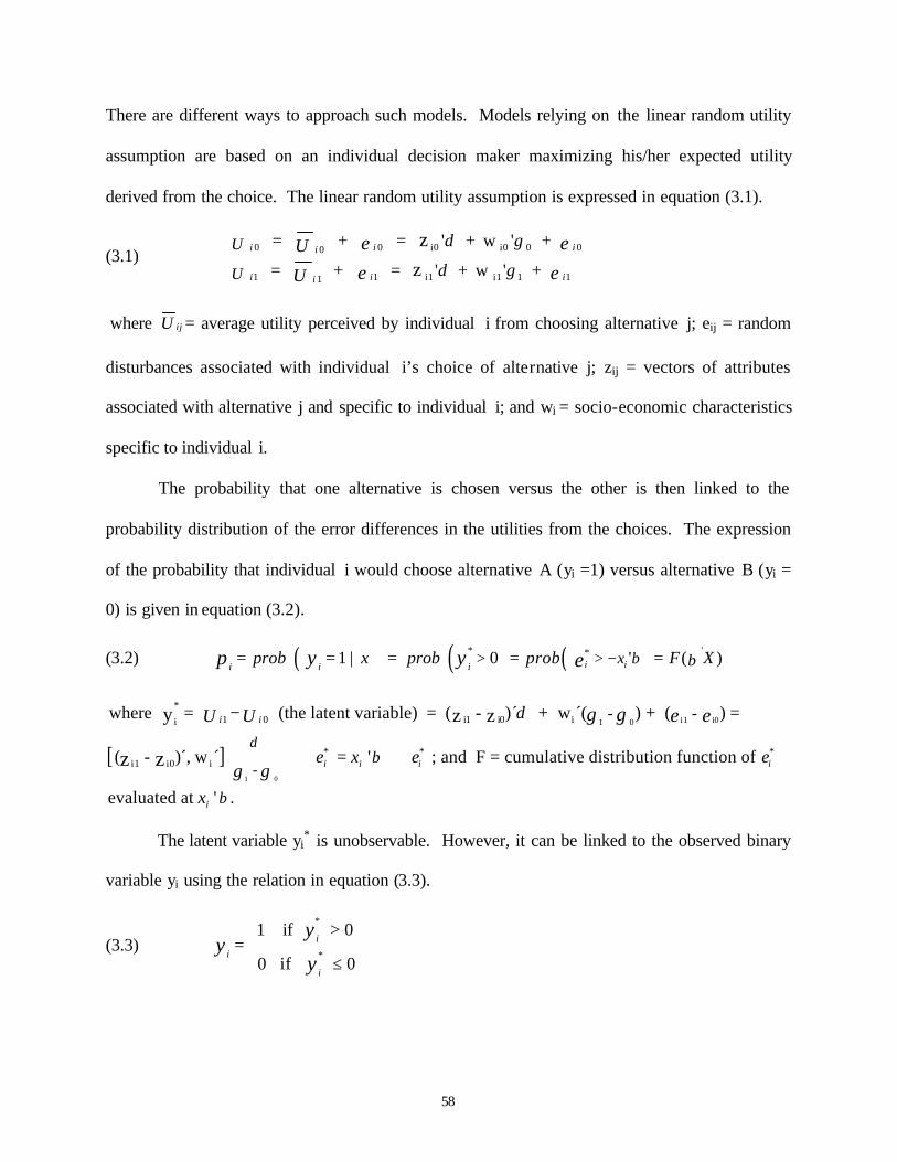
58
There are different ways to approach such models. Models relying on the linear random utility
assumption are based on an individual decision maker maximizing his/her expected utility
derived from the choice. The linear random utility assumption is expressed in equation (3.1).
(3.1) i0 i0 00 0 00
i1 i1 11 1 11
= + = ' + w ' +
= + = ' + w ' +
zz
i i ii
i i ii
U
U
U
U
e ee e
δ γ
δ γ
where ijU = average utility perceived by individual i from choosing alternative j; eij = random
disturbances associated with individual i’s choice of alternative j; zij = vectors of attributes
associated with alternative j and specific to individual i; and wi = socio-economic characteristics
specific to individual i.
The probability that one alternative is chosen versus the other is then linked to the
probability distribution of the error differences in the utilities from the choices. The expression
of the probability that individual i would choose alternative A (yi =1) versus alternative B (yi =
0) is given in equation (3.2).
(3.2) ( ) ( ) ( )* '* 1 | 0 ' ( ) iii i ixprob x prob prob F Xp y y e β β> > −= = = = =
[ ]1 0
i1 i01 0
*ii1 i01 0i
* *ii1 i0
-
- - where = (the latent variable) = ( - )´ + w ´( ) + ( ) =
( - )´, w ´ = ' ; and F = cumulative distribution function of
y z z
z z
i i
i i i ie x e e
U U e eδ
β
δ
γ γ
γ γ−
+ +
*
evaluated at ' .ix β
The latent variable yi* is unobservable. However, it can be linked to the observed binary
variable yi using the relation in equation (3.3).
(3.3) *
*
1 if 0
0 if 0
ii
i
yy
y
>= ≤
59
The interpretation of the relationship between a specific explanatory variable and the
outcome of the probability is different from the standard interpretation in multiple linear
regression. Indeed, in the multiple linear regression case, the parameter estimate accounts for the
changes in the dependent variable with respect to a change in the exogenous variable. Therefore,
a significant parameter would imply a significant effect on the dependent variable. The
nonlinearity in the binary response model, however, prevents such interpretation and requires a
different measure to summarize the effect of an explanatory variable. The partial change in the
probability of an event is called a marginal effect. It is obtained by taking the partial derivative
of the expression of the probability with respect to a change in the variable of interest.
Assumption of a specific form for the distribution of the error terms allows for computing
the probability of Y =1, given the explanatory variables X. The standard normal and logistic
distributions represent the two distributions frequently considered in discrete choice modeling.
Both distributions are symmetric and lead to probabilities confined to the unit interval.
3.3. Analytical Framework
The present study aims to analyze the likelihood of a dairy producer of a specific
description to adopt one or more technologies. The conduct of a probit analysis will allow for
estimating the probability of a dairy producer adopting a specific BMP, given the economic and
non-economic factors hypothesized as determinant in the decision to adopt and the assumption of
normal random errors associated with the random utility. Analysis of the coefficients and
marginal effects of significant explanatory variables establishes the relationship between the
explanatory variables and the conservation practices.
Findings of previous studies suggest the appropriateness of assuming contemporaneous
correlation between adoption equations of multiple management measures. Consequently,
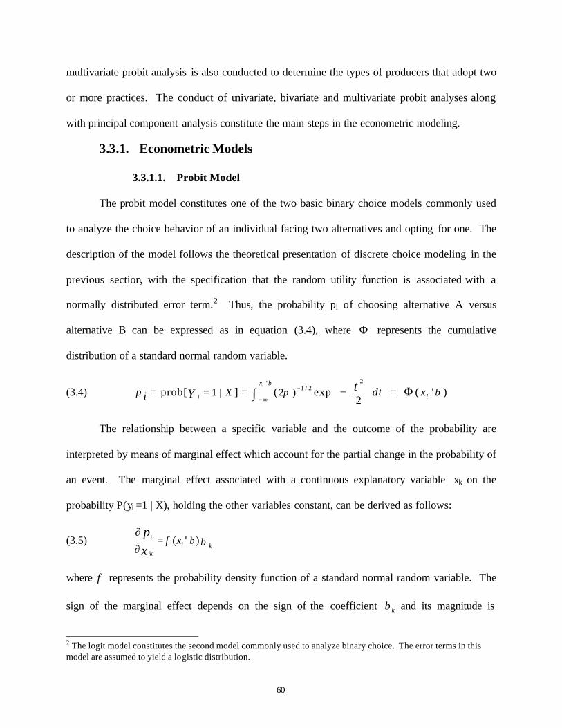
60
multivariate probit analysis is also conducted to determine the types of producers that adopt two
or more practices. The conduct of univariate, bivariate and multivariate probit analyses along
with principal component analysis constitute the main steps in the econometric modeling.
3.3.1. Econometric Models
3.3.1.1. Probit Model
The probit model constitutes one of the two basic binary choice models commonly used
to analyze the choice behavior of an individual facing two alternatives and opting for one. The
description of the model follows the theoretical presentation of discrete choice modeling in the
previous section, with the specification that the random utility function is associated with a
normally distributed error term.2 Thus, the probability pi of choosing alternative A versus
alternative B can be expressed as in equation (3.4), where Φ represents the cumulative
distribution of a standard normal random variable.
(3.4) 2'
1 / 21 | 2 )prob[ ] exp ( ' )(2i
ix
iX dt xp i Y tβ
βπ −
−∞=
= = − =
Φ∫
The relationship between a specific variable and the outcome of the probability are
interpreted by means of marginal effect which account for the partial change in the probability of
an event. The marginal effect associated with a continuous explanatory variable xk on the
probability P(yi =1 | X), holding the other variables constant, can be derived as follows:
(3.5) ( ' )ii k
ik
xpx
β βφ∂
=∂
where φ represents the probability density function of a standard normal random variable. The
sign of the marginal effect depends on the sign of the coefficient kβ and its magnitude is
2 The logit model constitutes the second model commonly used to analyze binary choice. The error terms in this model are assumed to yield a logistic distribution.
61
determined by the values of both kβ and X .β Consequently, the size of the effect depends on
the levels of all variables included in the X matrix. Different estimates of marginal effects can
be obtained from different values of the independent variables.
Estimates of marginal effects at the mean values of all independent variables constitute
the commonly reported summary measure in many studies. Such results are automatically
obtained using LIMDEP. However, they might be inappropriate if the X matrix includes dummy
variables. The mean value for a dummy variable is not suitable because it does not correspond to
any observable values (Long, 1997). Hence, it would be more appropriate to estimate the
marginal effects at specific values of the dummy variable while holding continuous variables at
their means. In this study, the value of a specific dummy variable included in the marginal effect
estimation was set to either 0 or 1 based on its mean value. Dummy variables with mean values
less than 0.5 were set to 0 and 1 otherwise.
Furthermore, discrete changes in the predicted probabilities constitute an alternative to
the marginal effect when evaluating the influence of a dummy variable d. Such effect can be
derived from equation (3.6).
(3.6) ( ) ( ), 1 , d =0X d Xβ β∆ = Φ = − Φ
In this analysis, three types of marginal effects were computed: at the mean values of all
variables; at specific values of the dummy variables; and assuming discrete changes for
significant dummy variables. The significance of a marginal effect was assessed using the delta
method as presented in the section, Special Computations and Tests.
3.3.1.2. Bivariate Probit Model
Discrete modeling that requires the inclusion of two equations with correlated
disturbances extends the probit model to what is known as the bivariate probit model. The basic
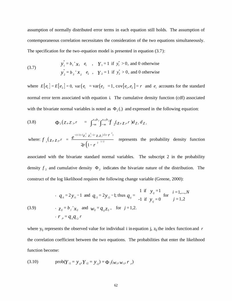
62
assumption of normally distributed error terms in each equation still holds. The assumption of
contemporaneous correlation necessitates the consideration of the two equations simultaneously.
The specification for the two-equation model is presented in equation (3.7):
(3.7)
* *1 1 1111
* *2 2222 2
' , 1 if 0, and 0 otherwise
, 1 if 0, and 0 otherwise'
e y
e y
y x Yxy Y
β
β
= + = >
= + = >
where [ ] [ ] ( ) ( ) [ ]1 2 1 2 1 20, var var 1, cov ,E Ee e e e e e ρ= = = = = and ie accounts for the standard
normal error term associated with equation i. The cumulative density function (cdf) associated
with the bivariate normal variables is noted as 2 (.)Φ and expressed in the following equation:
(3.8) ( ) 21 2 1 2 1
1 21 22 2, , , , ( ) i ix x
Z ZZ Z d dz zβ β
ρ ρφ−∞ −∞=Φ ∫ ∫
( )( )
22 21 2 1 2
2 (1 )
1 2 1 / 22 2
(1/2) ( ) /, ,
2 1where:
z z z zez zρ ρ
ρπ
φρ
+ − −−
=−
represents the probability density function
associated with the bivariate standard normal variables. The subscript 2 in the probability
density 2φ and cumulative density 2Φ indicates the bivariate nature of the distribution. The
construct of the log likelihood requires the following change variable (Greene, 2000):
(3.9)
1 1 2 2
* 1 2
1 if 1 1,...,2 1 and 2 1; thus for
1,2-1 if 0
' and , for 1,2.
ij
i i i i ijij
jij ijij ij ij
i i i
i Nj
j
yq y q y q
y
qx wz zq q
β
ρρ
•
•
•
= == − = − = ==
= = =
=
where yij represents the observed value for individual i in equation j, zij the index function and ρ
the correlation coefficient between the two equations. The probabilities that enter the likelihood
function become:
(3.10) 1 2 *1 2 21 2, ,prob( , ) ( )i i ii ii i w wy yY Y ρ= = = Φ
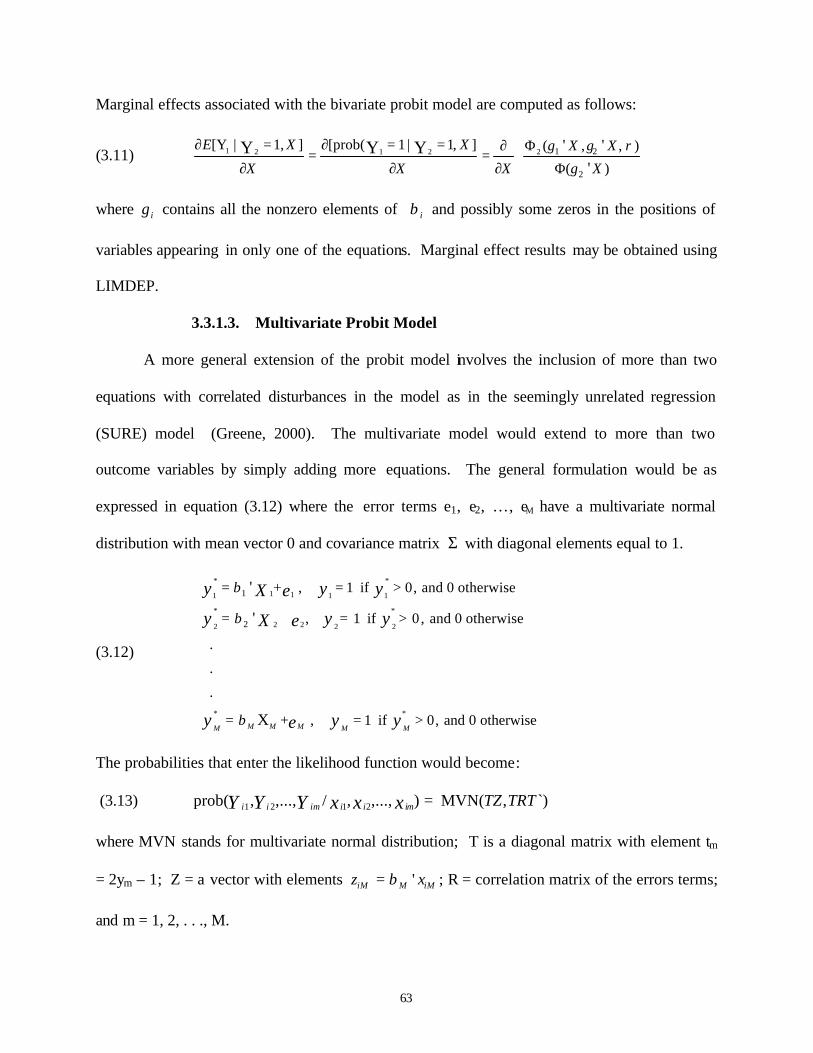
63
Marginal effects associated with the bivariate probit model are computed as follows:
(3.11) 1 2 1 2 2 1 2
2
[Y | 1, ] [prob( 1 | 1, ] ( , , )
( )
' ''
Y Y YE X X X X
X X X X
γ γ ρ
γ
∂ = ∂ = = Φ∂= =
∂ ∂ ∂ Φ
where iγ contains all the nonzero elements of iβ and possibly some zeros in the positions of
variables appearing in only one of the equations. Marginal effect results may be obtained using
LIMDEP.
3.3.1.3. Multivariate Probit Model
A more general extension of the probit model involves the inclusion of more than two
equations with correlated disturbances in the model as in the seemingly unrelated regression
(SURE) model (Greene, 2000). The multivariate model would extend to more than two
outcome variables by simply adding more equations. The general formulation would be as
expressed in equation (3.12) where the error terms e1, e2, …, eM have a multivariate normal
distribution with mean vector 0 and covariance matrix Σ with diagonal elements equal to 1.
(3.12)
* *
1 11 1 1
* *
2 22 2 2
* *
1
2
+ , 1 if 0, and 0 otherwise
, 1 if 0 , and 0 otherwise
.
.
.
+ , 1 if 0, and 0 otherwise
'
'
XM M MM M M
y y yeX
y y yeX
y y ye
β
β
β
= = >
= + = >
= = >
The probabilities that enter the likelihood function would become:
(3.13) 1 2 1 2prob( , ,..., / , ,..., ) MVN( , `)i i im i i im TZ TRTx x xY Y Y =
where MVN stands for multivariate normal distribution; T is a diagonal matrix with element tm
= 2ym – 1; Z = a vector with elements 'iM M iMz xβ= ; R = correlation matrix of the errors terms;
and m = 1, 2, . . ., M.
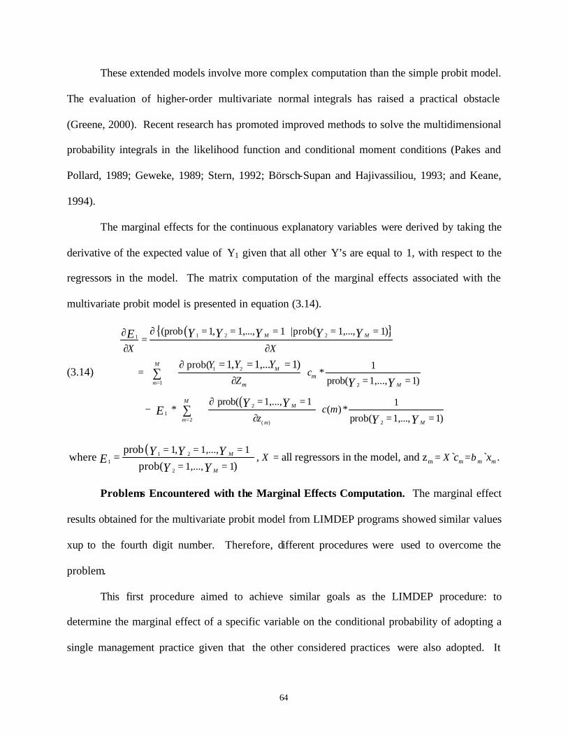
64
These extended models involve more complex computation than the simple probit model.
The evaluation of higher-order multivariate normal integrals has raised a practical obstacle
(Greene, 2000). Recent research has promoted improved methods to solve the multidimensional
probability integrals in the likelihood function and conditional moment conditions (Pakes and
Pollard, 1989; Geweke, 1989; Stern, 1992; Börsch-Supan and Hajivassiliou, 1993; and Keane,
1994).
The marginal effects for the continuous explanatory variables were derived by taking the
derivative of the expected value of Y1 given that all other Y’s are equal to 1, with respect to the
regressors in the model. The matrix computation of the marginal effects associated with the
multivariate probit model is presented in equation (3.14).
(3.14)
( ){ }
( )
1 2 21
1 2
1 2
21
( )
(prob 1, 1,..., 1 |prob( 1,..., 1)
prob( 1 *
prob( 1,..., 1)
prob( 1,..., 1 1 * ( ) *
p
1, 1,... 1)
M M
MM
m M
M
m
mm
X X
Yc
Z
c mz
Y Y
Y Y Y Y YE
Y Y
Y YE
=
∂ = = = = =∂=
∂ ∂
∂=
∂ = =
∂ = =−
∂
= = =
∑
2 2
rob( 1,..., 1)
M
m MY Y= = =
∑
( )1 21
2
m
1, 1,..., 1= =
1,..., 1
probwhere , all regressors in the model, and z ` ` .
prob( )M
M
m m mX X c xY Y YE
Y Yβ
= = ==
= ==
Problems Encountered with the Marginal Effects Computation. The marginal effect
results obtained for the multivariate probit model from LIMDEP programs showed similar values
xup to the fourth digit number. Therefore, different procedures were used to overcome the
problem.
This first procedure aimed to achieve similar goals as the LIMDEP procedure: to
determine the marginal effect of a specific variable on the conditional probability of adopting a
single management practice given that the other considered practices were also adopted. It
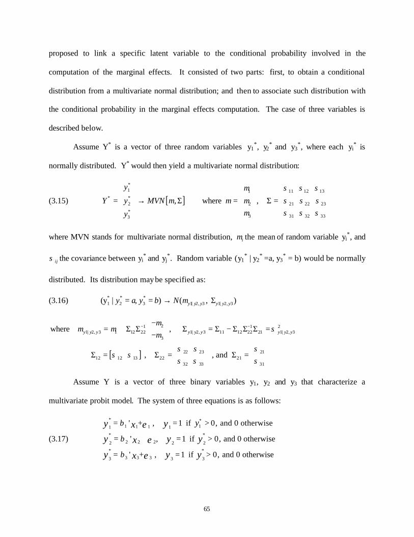
65
proposed to link a specific latent variable to the conditional probability involved in the
computation of the marginal effects. It consisted of two parts: first, to obtain a conditional
distribution from a multivariate normal distribution; and then to associate such distribution with
the conditional probability in the marginal effects computation. The case of three variables is
described below.
Assume Y* is a vector of three random variables y1*, y2
* and y3*, where each yi
* is
normally distributed. Y* would then yield a multivariate normal distribution:
(3.15) [ ]
*1 11 12 131
* *2 2 21 22 23
*3 31 32 333
, where ,
y
Y y MVN
y
σ σ σµ
µ µ µ σ σ σµ σ σ σ
= → Σ = Σ =
where MVN stands for multivariate normal distribution, iµ the mean of random variable yi*, and
ijσ the covariance between yi* and yj
*. Random variable (y1* | y2
* =a, y3* = b) would be normally
distributed. Its distribution may be specified as:
(3.16) * * *1 2 3 1| 2, 3 1| 2, 3(y | , ) ( , )y y y y y yy a y b N µ= = → Σ
[ ]
21 1 21| 2, 3 1 12 22 1| 2, 3 11 12 22 21 1| 2, 3
3
22 23 2112 12 13 22 21
3132 33
where ,
, , and
y y y y y y y y y
µµ µ σ
µ
σ σ σσ σ
σσ σ
− −− = + Σ Σ Σ = Σ − Σ Σ Σ = −
Σ = Σ = Σ =
Assume Y is a vector of three binary variables y1, y2 and y3 that characterize a
multivariate probit model. The system of three equations is as follows:
(3.17)
* *1 11 11 1
* *2 2 22 2 2
* *3 3 33 3 3
' + , 1 if 0, and 0 otherwise
' , 1 if 0, and 0 otherwise
' + , 1 if 0, and 0 otherwise
yy yxy y yxy y yx
β
β
β
ε
ε
ε
= = > = + = >
= = >
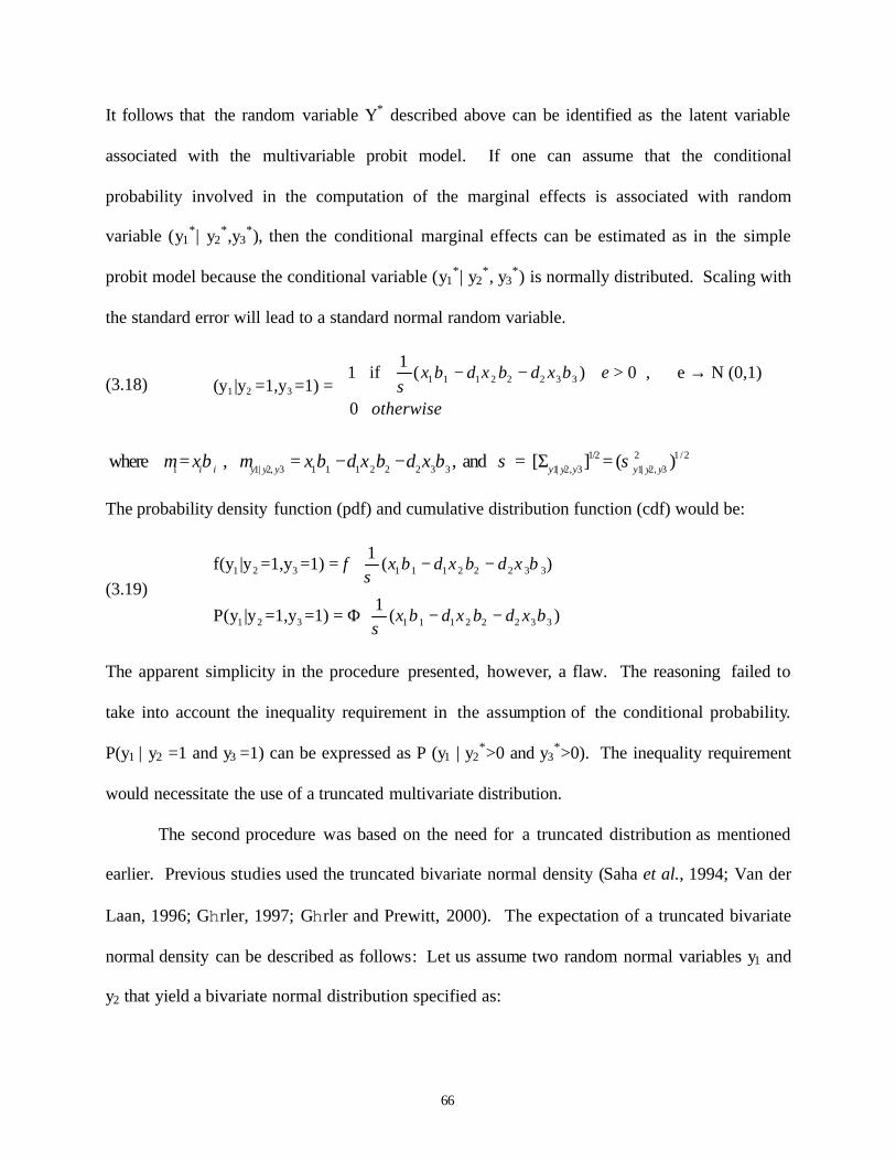
66
It follows that the random variable Y* described above can be identified as the latent variable
associated with the multivariable probit model. If one can assume that the conditional
probability involved in the computation of the marginal effects is associated with random
variable (y1*| y2
*,y3*), then the conditional marginal effects can be estimated as in the simple
probit model because the conditional variable (y1*| y2
*, y3*) is normally distributed. Scaling with
the standard error will lead to a standard normal random variable.
(3.18) 1 1 1 2 2 2 3 31 2 3
11 if ( ) 0 , e N (0,1)
(y |y =1,y =1) = 0
x x x e
otherwise
β δ β δ βσ
− − + > →
1/2 2 1 /2i 1| 2, 3 1 1 1 2 2 2 3 3 1| 2, 3 1| 2, 3where = , , and = [ ] = ( )i i y y y y y y y y yx x x xµ β µ β δ β δ β σ σ= − − Σ
The probability density function (pdf) and cumulative distribution function (cdf) would be:
(3.19) 1 2 3 1 1 1 2 2 2 3 3
1 2 3 1 1 1 2 2 2 3 3
1f(y |y =1,y =1) = ( )
1P(y |y =1,y =1) = ( )
x x x
x x x
φ β δ β δ βσ
β δ β δ βσ
− − Φ − −
The apparent simplicity in the procedure presented, however, a flaw. The reasoning failed to
take into account the inequality requirement in the assumption of the conditional probability.
P(y1 | y2 =1 and y3 =1) can be expressed as P (y1 | y2*>0 and y3
*>0). The inequality requirement
would necessitate the use of a truncated multivariate distribution.
The second procedure was based on the need for a truncated distribution as mentioned
earlier. Previous studies used the truncated bivariate normal density (Saha et al., 1994; Van der
Laan, 1996; Ghrler, 1997; Ghrler and Prewitt, 2000). The expectation of a truncated bivariate
normal density can be described as follows: Let us assume two random normal variables y1 and
y2 that yield a bivariate normal distribution specified as:
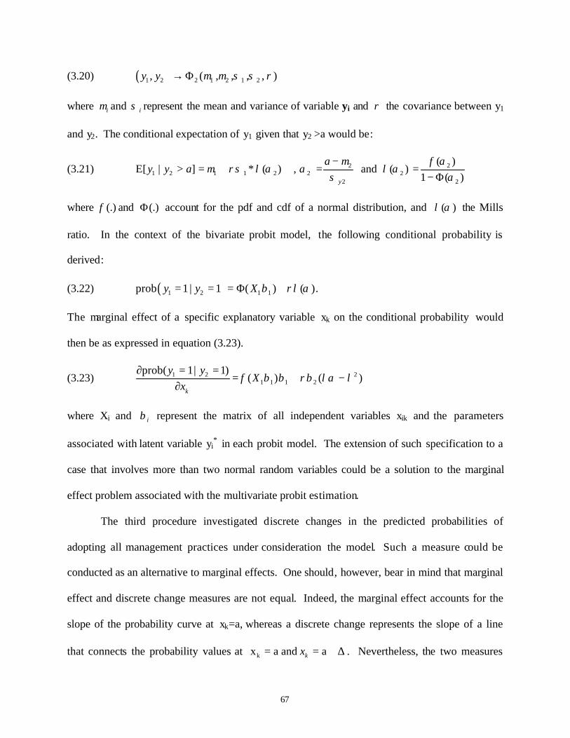
67
(3.20) ( )1 2 2 1 2 1 2, ( , , , , )y y µ µ σ σ ρ→ Φ
where iµ and iσ represent the mean and variance of variable yi and ρ the covariance between y1
and y2. The conditional expectation of y1 given that y2 >a would be:
(3.21) 2 21 2 1 1 2 2 2
2 2
( )E[ | ] * ( ) , and ( )
1 ( )y
ay y a
µ φ αµ ρσ λ α α λ α
σ α−
> = + = =− Φ
where (.)φ and (.)Φ account for the pdf and cdf of a normal distribution, and ( )λ α the Mills
ratio. In the context of the bivariate probit model, the following conditional probability is
derived:
(3.22) ( )1 2 1 1prob 1 | 1 ( ) ( ).y y X β ρλ α= = = Φ +
The marginal effect of a specific explanatory variable xk on the conditional probability would
then be as expressed in equation (3.23).
(3.23) 21 21 1 1 2
prob( 1| 1)( ) ( )
k
y yX
xφ β β ρβ λα λ
∂ = == + −
∂
where Xi and iβ represent the matrix of all independent variables xik and the parameters
associated with latent variable yi* in each probit model. The extension of such specification to a
case that involves more than two normal random variables could be a solution to the marginal
effect problem associated with the multivariate probit estimation.
The third procedure investigated discrete changes in the predicted probabilities of
adopting all management practices under consideration the model. Such a measure could be
conducted as an alternative to marginal effects. One should, however, bear in mind that marginal
effect and discrete change measures are not equal. Indeed, the marginal effect accounts for the
slope of the probability curve at xk=a, whereas a discrete change represents the slope of a line
that connects the probability values at kx a and akx= = + ∆ . Nevertheless, the two measures
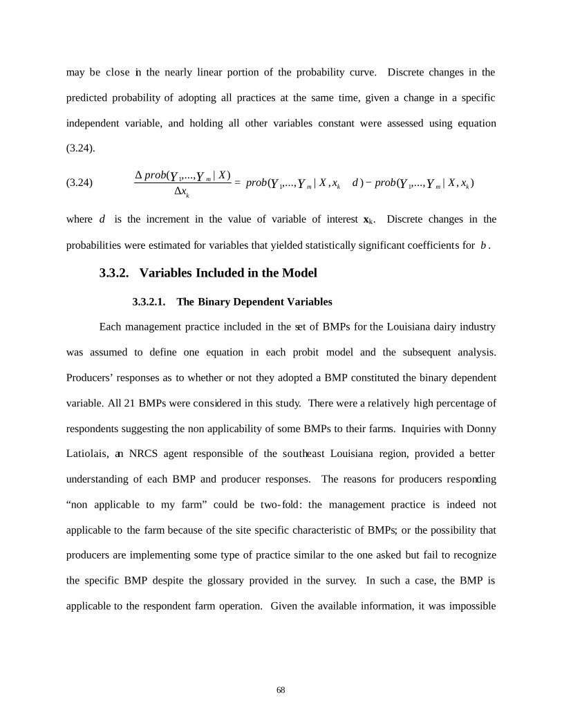
68
may be close in the nearly linear portion of the probability curve. Discrete changes in the
predicted probability of adopting all practices at the same time, given a change in a specific
independent variable, and holding all other variables constant were assessed using equation
(3.24).
(3.24) 11 1
( ,..., | ) ( ,..., | , ) ( ,..., | , )m
k km mk
prob Xprob X x prob X x
xY Y Y Y Y Yδ
∆= + −
∆
where δ is the increment in the value of variable of interest xk. Discrete changes in the
probabilities were estimated for variables that yielded statistically significant coefficients for .β
3.3.2. Variables Included in the Model
3.3.2.1. The Binary Dependent Variables
Each management practice included in the set of BMPs for the Louisiana dairy industry
was assumed to define one equation in each probit model and the subsequent analysis.
Producers’ responses as to whether or not they adopted a BMP constituted the binary dependent
variable. All 21 BMPs were considered in this study. There were a relatively high percentage of
respondents suggesting the non applicability of some BMPs to their farms. Inquiries with Donny
Latiolais, an NRCS agent responsible of the southeast Louisiana region, provided a better
understanding of each BMP and producer responses. The reasons for producers responding
“non applicable to my farm” could be two-fold: the management practice is indeed not
applicable to the farm because of the site specific characteristic of BMPs; or the possibility that
producers are implementing some type of practice similar to the one asked but fail to recognize
the specific BMP despite the glossary provided in the survey. In such a case, the BMP is
applicable to the respondent farm operation. Given the available information, it was impossible
69
to sort out the stated “non applicability” responses according to these two reasons. Thus,
producers answering “BMP Not Applicable to My Farm” was treated as not adopting the BMP.
The 21 management practices were grouped into four main categories for the purpose of
multivariate probit analysis, based on the primary objective of each management practice.
Eleven practices aimed to control erosion and sediment. Five practices focused on the
management of facility wastewater and runoff. Nutrient and pesticide management formed a
separate group. Three management practices were related to grazing management. A summary
of these variables is presented in Table 3.1. The producer’s response regarding his current
adoption of each management practice defined the binary dependent variable that took the value
of one if the BMP was currently implemented and zero otherwise. The unobservable latent
variable y* associated with each binary variable was assumed to be a linear function of the
hypothesized independent variables described in the next section.
3.3.2.2. The Explanatory Variables Included in the Analysis
A number of factors were hypothesized to affect the probability of adopting a specific
management practice. Such factors included farm attributes, dairy producer characteristics,
institutional variables and dairy producer’s attitude toward risk and the environment. Thirty-two
independent variables displayed in Table 3.2 were included as determinant of dairy farmers’
decision making with regard to the implementation of conservation practices.
3.3.2.2.1. Farm Attributes
Larger sized farms have generally been associated with an increased likelihood to adopt
technology (Westra and Olson, 1997; El-Osta and Morehart, 1999; Davis and Gillespie, 2000).
Adoption of a new technology often involves high initial outlay and farmers with greater
resources are better able to afford the technology. As Feder et al. (1985) stated, “the theoretical

70
Table 3.1. Binary Dependent Variables in the Analyses.
Categories Management Practices
Erosion and Sediment Control Practices 1. Conservation Tillage Practices 2. Cover and Green Manure Crop 3. Critical Area Planting 4. Field Borders 5. Filter Strips 6. Grassed Waterways 7. Heavy Use Area Protection 8. Regulating Water in Drainage System 9. Riparian Forest Buffer 10. Sediment Basin 11. Streambank and Shoreline Protection Facility Wastewater and Runoff Management 1. Roof Runoff Mangement 2. Waste Management System 3. Waste Storage Facility 4. Waste Treatment Lagoon 5. Waste Utilitzation
Nutrient and Pesticide Management 1. Nutrient Management 2. Pest Management Grazing Management 1. Fence 2. Prescribed Grazing 3. Trough or Tank
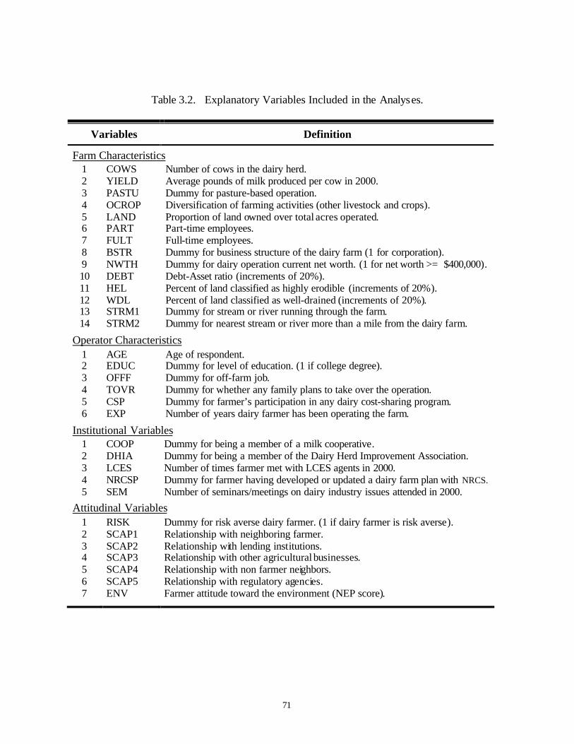
71
Table 3.2. Explanatory Variables Included in the Analyses.
Variables Definition
Farm Characteristics 1 COWS Number of cows in the dairy herd. 2 YIELD Average pounds of milk produced per cow in 2000. 3 PASTU Dummy for pasture-based operation. 4 OCROP Diversification of farming activities (other livestock and crops). 5 LAND Proportion of land owned over total acres operated. 6 PART Part-time employees. 7 FULT Full-time employees. 8 BSTR Dummy for business structure of the dairy farm (1 for corporation). 9 NWTH Dummy for dairy operation current net worth. (1 for net worth >= $400,000). 10 DEBT Debt-Asset ratio (increments of 20%). 11 HEL Percent of land classified as highly erodible (increments of 20%). 12 WDL Percent of land classified as well-drained (increments of 20%). 13 STRM1 Dummy for stream or river running through the farm. 14 STRM2 Dummy for nearest stream or river more than a mile from the dairy farm.
Operator Characteristics 1 AGE Age of respondent. 2 EDUC Dummy for level of education. (1 if college degree). 3 OFFF Dummy for off-farm job. 4 TOVR Dummy for whether any family plans to take over the operation. 5 CSP Dummy for farmer’s participation in any dairy cost-sharing program. 6 EXP Number of years dairy farmer has been operating the farm.
Institutional Variables 1 COOP Dummy for being a member of a milk cooperative. 2 DHIA Dummy for being a member of the Dairy Herd Improvement Association. 3 LCES Number of times farmer met with LCES agents in 2000. 4 NRCSP Dummy for farmer having developed or updated a dairy farm plan with NRCS. 5 SEM Number of seminars/meetings on dairy industry issues attended in 2000.
Attitudinal Variables 1 RISK Dummy for risk averse dairy farmer. (1 if dairy farmer is risk averse). 2 SCAP1 Relationship with neighboring farmer. 3 SCAP2 Relationship with lending institutions. 4 SCAP3 Relationship with other agricultural businesses. 5 SCAP4 Relationship with non farmer neighbors. 6 SCAP5 Relationship with regulatory agencies. 7 ENV Farmer attitude toward the environment (NEP score).
72
literature suggests that large fixed costs cause a reduced tendency to adopt and a slower rate of
adoption on smaller farms.” Furthermore, even size neutral techno logies may be more heavily
adopted by larger farmers if the costs associated with learning are appropriated as fixed expenses
(Feder et al., 1985). Total number of cows in the dairy herd (COWS) was used as a proxy for
farm size in this study. Larger dairy farms were hypothesized to be more involved in wastewater
and runoff management to better handle the large amount of manure and waste produced on their
farms.
Farm productivity may reflect producers’ openness to new technology that provides
greater productivity gains (Ghosh et al., 1994; Zepeda, 1994; El-Osta and Morehart, 1999). It
characterizes farm operator management ability. Farm productivity has usually been
incorporated in technological adoption studies as an endogenous variable because technology
affects productivity. El-Osta and Morehart (1999) considered YIELD as a determinant factor in
the adoption of advanced milking parlors and DHIA technology in the U.S. dairy industry, and
used an instrument variable for yield to deal with the endogeneity problem. Zepeda (1994)
included dairy farm productivity as one of the three endogenous variables in the simultaneous
equations of adopting DHIA. In this study, cow productivity was not considered as an
endogenous variable because conservation management practices target primarily the
enhancement of the environment, not farm production. Therefore, the productivity variable was
included as an exogenous determinant of BMP adoption. Average pounds of milk per cow
(YIELD) was incorporated as an explanatory variable to account for the differential ability of the
productive farm to bear the fixed adoption costs of conservation management as high
productivity would likely ensure larger profits.
73
Diversification in farming activities is a risk management strategy, one of the common
tools for managing agricultural risks associated with yield, price and income (Fleisher, 1990;
Anderson and Dillon, 1992). Hence, risk aversion would drive farmers to engage in alternative
enterprises. Fernandez-Cornejo et al. (1994) included output diversification as one proxy of risk
aversion in their study of the adoption of integrated pest management techniques by vegetable
growers in Florida, Michigan and Texas. They found a significant positive relationship between
the diversification variable and farmers’ adoption of the technique. In this study, producers
engaged in diverse agricultural enterprises were hypothesized to likely adopt management
practices relevant to each type of activity. Variable (OCROP) was included to account for the
number of other farming activities in which the dairy farmer was involved besides milk
production and raising hay. It was hypothesized to be positively correlated with the probability
to adopt a BMP.
The effect of land tenure has been examined in many technology adoption studies. Soule
et al. (2000) emphasized the importance of land tenure in farmer’s adoption of conservation
practices and the negative association between adoption and variable “renter” of land. Cardona
(1999) also pointed out sugarcane farmers’ unwillingness to implement BMPs on rented land,
showing a negative relationship between adoption and the variable “tenure”. Fernandez-Cornejo
et al. (1994) provided a discussion on the likelihood of land ownership to influence adoption of
innovations requiring investments tied to the land. Tenants’ lack of motivation to adopt would
be due to the perception of benefits accruing to the landowner, and not to the renter. In this
study, the proportion of owned land to total acres operated (LAND) was included. A greater
fraction of land owned was hypothesized to increase the adoption of soil management practices.
74
Respondents were asked whether their operation was a pasture-based operation or a free-
stall operation. In pasture-based operations, cows are allowed to graze much of the day on
forages. A free-stall operation differs from the pasture-based operation in that it includes
separate areas for milking, feeding and lounging, all generally inside the structure on cement.
Animals are not allowed to graze on forage. Both pasture-based and free-stall dairy farms were
expected to be involved in the runoff and waste management practices. Dairy farms more
involved in grazing activity were assumed to have information about grazing management
practices. Pasture-based operation was included as dummy variable (PASTU) that took the value
of one if the operation was forage based and zero otherwise. It was hypothesized to enhance the
adoption of grazing management practices.
As discussed by Feder et al. (1985), labor availability may affect a farmer’s decision to
adopt technology. Labor shortages promote the adoption of labor-saving practices, but hinder
the implementation of technologies that require more labor input. The number of part-time
(PART) and full time (FULT) employees were included as explanatory variables. A greater
labor force was hypothesized to increase the adoption of labor demanding conservation practices
such as waste management, nutrient management and pesticide management. On the other hand,
some labor saving practices might include conservation tillage.
Business structure constitutes a decision factor that is likely to impact the adoption of
management practices. The corporate farm structure allows producers to take greater investment
risk than sole proprietors. Furthermore, sole proprietors are likely older farm operators with
shorter planning horizons, and therefore, less willing to adopt technology (El-Osta and Morehart,
1999, p. 88). Business structured as a farm corporation was included as a dummy variable
75
(BSTR) which took the value of one for a corporate farm and zero otherwise. BSTR was
hypothesized to increase the adoption of BMPs.
A dairy farmer’s financial situation could also impact his decision as to whether to incur
greater costs by implementing management practices. Dairy operations with greater net worth
are farms with greater resources, able to afford the costs of implementing a BMP. Current dairy
operation net worth (NWTH) was included as a dummy variable that took the value of one if the
farm net worth was at least $400,000, which described the level of net worth of a medium sized
dairy farm.
Debt-asset ratio (DEBT) is critical in a dairy farmer’s financial decision making. Higher
debt that is most likely borne by turnkey and established dairy farms may indicate two different
things. The debt could be the result of an increased investment from a recent adoption of
technology. In such a case, the debt variable would positively affect the adoption of BMPs. On
the other hand, a high debt load could be an impediment to new BMP implementation because
the farm operator would be reluctant to increase his or her liabilities. Thus, a high debt-asset
ratio would be less likely to increase adoption. The ambiguous effects of debt-to-asset ratio on
adoption were discussed by Fernandez-Cornejo et al. (1994). They found higher debt/asset
ratios associated with an increased adoption of integrated pest management by vegetable growers
in Florida and Texas, and a negative effect on growers in Michigan. Gould et al. (1989) found a
negative association of debt ratio and adoption of conservation tillage in Wisconsin. In this
study, the sign of variable DEBT is to be explored.
The four remaining farm attribute variables relate to the physical characteristics of the
farmer’s land. Operators with land classified as highly erodible would have a greater need to
carry out soil conservation practices. Thus, variable HEL, which accounts for the percentage of
76
the farmer’s land classified as highly erodible, was included to capture this effect. The drainage
characteristics of the land is important in farming activities. The drainage variable would affect
some BMP adoption more than others. Dairy farmers who have poorly drained areas may opt to
improve their drainage system through water control structures. Variable WDL measured the
percentage of the farmer’s land classified as well-drained. WDL was hypothesized to
specifically increase the implementation of erosion and sediment control practices.
Two dummy variables were included to account for the existence of a stream and/or river
on the dairy farm or nearby. Variable STRM1 took the value of one if a stream and/or river ran
through the farm. Variable STRM2 took into consideration the existence of the nearest stream or
river distant from the farm, taking the value of one if the nearest stream or river was more than
one mile away from the dairy farm and zero otherwise. STRM1 variable was expected to
increase the implementation of BMPs, especially those such as streambank and shoreline
protection, whereas STRM2 would likely reduce the adoption of BMPs.
3.3.2.2.2. Dairy Operator Characteristics
Six variables that describe dairy operators in Louisiana were considered in the
econometric model. The roles of age and educational attainment in farmers’ decisions to adopt
technology have been shown in previous studies (Feder et al., 1985; Gould et al., 1989; Shields
et al., 1993; Zepeda, 1994; Dorfman, 1996; Westra and Olson, 1997; Cardona, 1999; El-Osta and
Morehart, 1999; Soule et al., 2000). Both variables were included. Variable AGE accounted for
the age of the primary operator and was hypothesized to negatively affect farmers’ adoption of
BMPs because older operators with shorter planning horizons would be less inclined to adopt
new technologies. Dummy variable EDUC accounted for level of education. It took the value of
one if the dairy farmer held a college degree and zero otherwise. Educational attainment was
77
expected to improve the decision-making process and enhance adoption. Consequently, EDUC
was hypothesized to have a positive sign.
Other factors such as holding an off- farm job (OFFF), having family members who plan
to take over the operation upon the farmer’s retirement (TOVR), and participation in a dairy
cost-sharing program (CSP) such as EQIP were assessed and included as dummy variables.
Each variable took the value of one if the producer responded “yes” to the related question in the
survey, and zero otherwise. As Feder et al. (1985) suggested, off- farm income would permit
farmers to overcome the capital constraint and carry out agricultural practices. Hence, variable
OFFF was expected to have a positive sign. The existence of family plans to take over the
operation upon the farmer’s retirement in effect would extend farmers’ planning horizons. It
would encourage the adoption of conservation practices as farm operators would have an
incentive to maintain productivity of soil for future generations (Gould et al., 1989) Therefore,
TOVR was expected to increase the adoption of BMPs. Participation in cost-sharing programs
likely increases producer involvement in governmental conservation programs. Therefore,
variable CSP was expected to be associated with a positive sign.
The last variable that characterizes the dairy producer accounts for his experience in dairy
farming. The number of years the dairy farmer had been operating the farm (EXP) was included
to capture the increased effect of experience on the adoption decision. Similar to education,
experience was expected to improve farmers’ ability to adopt new technologies.
3.3.2.2.3. Institutional Variables
Adoption decision making evolves within a multi-stage process where information plays
a major role (Freda and Shields, 1980; Anderson, 1993; Moser and Barrett, 2002). A farmer’s
decision to adopt a management practice is shaped by different sources of information. Training
78
programs provided primarily by the Natural Resource Conservation Service (NRCS) and the
Louisiana Cooperative Extension Service (LCES) via programs such as the Modern Farmer
Program, would constitute dairy farmers’ sources of information regarding environmental issues
related to agricultural activities and potential solutions to such problems. More frequent
meetings with extension agents would indicate the farmer’s reliance on the type of information
provided and the likely subsequent acceptance of the recommended practices. Thus, the number
of times the farmer met with extension agents in 2000 (LCES) was included as an explanatory
variable to capture the increased adoption effect. A dairy farm plan developed with NRCS
would suggest the farmer’s willingness to comply with environmental standards and, therefore,
to adopt conservation practices. Such information was incorporated as a dummy variable
(NRCSP) that took the value of one if a plan was developed or updated with NRCS and zero
otherwise.
Other sources of information included dairy cooperatives and associations as well as the
mass media. A farmer’s awareness of other dairy operators’ experiences was likely to be
important in deciding whether to adopt technology. Many cooperatives promote communication
among dairy producers and provide cooperative members information through newsletters,
quarterly meetings or other activities. Thus, a dummy variable (COOP) to account for being a
member of a dairy cooperative was included. Producers who are better record keepers were also
hypothesized to be more willing to adopt conservation practices since they were likely to be
more progressive farmers. Dummy variable (DHIA) accounted for being member of the Dairy
Herd Improvement Association. DHIA was hypothesized to positively influence the decision to
adopt.

79
Gathering information through seminars and meetings that deal with dairy industry issues
constitutes another source of information for dairy farmers. Greater concern for industry issues
is likely to enhance adoption of technologies. Number of seminars and/or meetings attended in
2000 (SEM) was expected to positively influence the farmer’s decision to adopt.
3.3.2.2.4. Attitudinal Variables
Thurstone’s (1928) view of attitude as a multidimensional psychological construct that
embraces all inclinations and feelings an individual experiences toward a specific subject has
been well accepted and restated in attitudinal research literature. The broad extent of liking or
disliking something establishes the complex aspect of human attitude. Over time, research
findings have emphasized the rationale for linking individual’s attitude and behavior (Albrecht
and Carpenter, 1976; Werner, 1977; Mueller, 1986; Arcury and Christianson, 1990; Arcury,
1990; Stern et al., 1995; Schultz and Oskamp, 1996). Mueller concluded ‘…people would
routinely behave according to their attitudes and predispositions.’ (Mueller, 1986: p. 98).
Unidimensional concepts were developed to account for a particular aspect of a human
being’s attitude and narrow down the focus to a specific attitudinal object. Seven specific
attitudinal variables were included in this study. One variable relates to a dairy farmer’s attitude
toward risk, another relates to his attitude toward the environment, and five variables describe his
social relationships with neighbors, as well as financial and regulatory institutions relevant to
dairying activities.
Risk and uncertainty have been discussed in previous empirical studies as impeding
factors to technology adoption (Shields et al, 1993; Ghosh et al., 1994; Fernandez-Cornejo et al.,
1994; Feder et al., 1994; Krause and Black, 1995). These factors urge the risk averse farmer to
selectively adopt technology that ensures net expected marginal benefits. In this study,
80
producer’s risk aversion was estimated based on the subjective assessment of whether they took
substantial levels of risk, neither seek nor avoid risk, or tended to avoid risk whenever possible in
their investment decisions. Variable RISK was included as a dummy variable that took the value
of 1 if farmer tended to avoid risk and zero otherwise. RISK was expected to increase the
adoption of BMPs that reduce soil runoff, insuring long-run viability of land. For some BMPs
such as conservation tillage, however, the hypothesized sign may be ambiguous, since
conventional tillage has been shown in some uses to reduce yield variability.
Farmer’s behavior toward the environment was assessed based on the New
Environmental Paradigm (NEP) scale developed by Dunlap et al. in 2000. The pool of items
considered in the NEP scale includes 15 statements to elicit opinions on five hypothesized
features of an ecological worldview, and locate the individual’s position on an affective
continuum, from a “very positive” to a “very negative” attitude toward the pro-ecological view.
The statements are worded in such a way that agreement with the eight odd-numbered items and
disagreement with the seven even-numbered ones would denote a pro-ecological worldview.
Variable ENV described the NEP score associated with the dairy operator’s environmental
attitude. It accounted for the dairy producer’s average score over the 15 statements. It was
expected that environmental concern would drive the farm operator to implement conservation
practices.
The concept of social capital, introduced by Bourdieu in 1983 and later developed by
Coleman (1988), has received researchers’ interest over the past two decades. Social capital has
been defined in many ways. Coleman emphasized that “social capital is defined by its function.
It consists of different entities with two elements in common: the social structure aspects and the
facilitation of certain actions of actors.” Putman (1995) defined social capital as “the features of
81
social organization, such as networks, norms and social trust, that facilitate coordination and
cooperation for mutual benefits.” Although researchers have attempted to describe the concept
while emphasizing a specific aspect or dimension of social capital in human action, the general
perception of social capital as an aggregate concept based on individual’s social networks and
relationships is well accepted (Coleman, 1988; Putman, 1995; Brehm,1997; Burt, 1997; Paxton,
1999; Schmid, 2000). Research findings have emphasized the critical role of inherent social
capital in networks and organizations in community and economic development (Bebbington,
1997; Grant, 2001). Trusting and positive network relationships as well as availability of
information inherent in social relations would increase individual capacity for action.
Economists have acknowledged the role of social capital in the conduct of business
transactions. Schmid and Robison (1995) defined social capital as “a productive asset which is a
substitute for and complement to other productive assets.” Peterson et al. (1999) discussed the
role of trust, reputation and affiliation in creating different types of social capital between
business partners. Trust built upon repeated transactions between business partners would
influence the establishment of direct social capital. Consistent and reliable transactions would
develop reputations, and association affiliation or acquaintanceship would reinforce the
establishment of a trusting relationship.
A dairy operator’s perception of his social relationships with neighboring farmers
(SCAP1), lending institutions (SCAP2), other agricultural businesses (SCAP3), non farmer
neighbors (SCAP4) and regulatory agencies (SCAP5) was hypothesized to affect his decision to
adopt management practices. The farmer’s assessment of his relation with each entity as “not
important”, “not very important”, “somewhat important” and “very important” was scored 0, 1,
2, or 3, respectively. SCAP2 and SCAP5 were hypothesized to increase the adoption of BMPs
82
since important relationships with lending institutions would ensure financial support for the
required investment and important relationships with regulatory agency would provide better
information regarding the necessity to implement specific management practices. The
remaining social capital variables SCAP1, SCAP3 and SCAP4 were included for exploratory
purposes.
3.4. Special Computations and Tests
3.4.1. Testing for Multicollinearity
Collinearity problems have received much attention from researchers dealing with
multivariate analysis. Collinearity among multiple explanatory variables included in an analysis
can impair the interpretation of the effects of a specific variable due to the lack of variability in
the data or a nearly exact linear interrelationship among explanatory variables (Judge et al.,
1988; Hair et al., 1998). Testing for multicollinearity and taking the appropriate measures to
minimize the problem are usually among the first steps in econometric analysis. A collinear
relationship between two variables can be ascertained by examining the values of the correlation
coefficients and using the rule of thumb of greater than or equal to 0.8 to specify a strong linear
association between the two variables.
In the case of multiple variables, it would be more appropriate to investigate the
condition indexes associated with the characteristic roots or eigenvalues of the matrix X’X where
the X matrix takes into account all the explanatory variables in the model. The condition index
can be evaluated using equation (3.25)
(3.25) 1 / 2
ii
k
CIλλ
=
83
where λi accounts for a specific eigenvalue i, and λk represents the largest eigenvalue. A value
of the ratio between 30 to 100 or above 100 would indicate a strong or very strong collinearity
problem, respectively. The study of the variance proportions matrix allows one to identify the
variables associated with the large condition indexes and take appropriate measures to correct the
collinearity problem. Diagnostics for multicollinearity were performed using SAS.
3.4.2. Principal Component Analysis (PCA)
PCA was used in this analysis to scale down the large number of potentially relevant
explanatory variables included in the empirical model. The use of all 32 variables in the
multivariate probit analysis would lead to the problem of too few degrees of freedom and
therefore, required the need for fewer variables.
PCA consists of a multivariate technique for examining relationships among several
quantitative variables. It allows for exposing linear relationships among a larger set of variables
and obtaining fewer uncorrelated components which retain much of the information in the
original data (Rao, 1964; Jolliffe, 1972 and 1973; Isebrands and Crow, 1975; Daultrey, 1976;
Fomby et al., 1984, Basilevsky, 1994; Hutcheson and Sofroniou, 1999). The PCA technique
associates each component to a weighted linear combination of the original variables where the
eigenvectors of the correlation or covariance matrix are the coefficients in such linear
combination and the eigenvalues of the matrix account for the variance of each component.
The fundamental question in PCA is how to select the components that best describe the
structure of the inter-correlations among the original set of variables and discard the remaining
components. Different methods have been proposed for discarding variables. Fomby et al.
(1984) discussed two methods. The first method simply suggests deleting principal components
associated with relatively small characteristic roots. Given that the variations in the data are
84
measured by the characteristic roots, such a technique would still preserve as much variation in
the data as before. However, the limitation of the method lies in its inability to provide insight
on the appropriateness of the restrictions. The second method emphasizes sequential test
restrictions implied by deleting components with increasingly large characteristic roots.
Jolliffe (1972 and 1973) investigated the problem of discarding variables using PCA on
artificial and actual data. Among other methods, his suggestion of associating one variable with
each of the first p components and retaining these variables seemed to give satisfactory results,
especially with actual data. The value of p can be set equal to either the number of eigenvalues
derived from the correlation matrix greater than λ0 or the number of components necessary to
account for some proportion of the total variation 0 .α Jolliffe’s findings advocated a suitable
level of λ0 equal to 0.7, but no acceptable value for 0 .α Daultrey (1976) also found an optimum
value for λ0 equal to 0.7 in his analysis of the post-War changes in agricultural structure in the
Republic of Ireland. Hutcheson and Sofroniou (1999) reported that, “the easiest and most
commonly used method is to select any component associated with an eigenvalue greater than
1.0.” However, they emphasized the absence of firm rules to establish the optimum number of
components, and drew attention to the need for a balance between the amount of variance
accounted for and the number of interpretable components.
In this study, two different levels of λ0 were selected to reduce the number of explanatory
variables in the econometric models and dispose of enough degrees of freedom in the estimation.
The basic rule for selecting variables considered for the bivariate probit analysis was λ0 = 0.7,
allowing for the retention of 17 explanatory variables. As more equations were added in the
multivariate probit model, a further reduction of the number of variables was crucial. The value
85
of λ0 was set to 1, yielding 12 variables. Joint tests on the discarded variables were conducted to
ascertain the variable selection.
3.4.3. LM Test for Heteroskedasticity
The assumption of homoskedastic error terms is one of the key assumptions in
econometric modeling. Errors across observations are assumed to be uncorrelated and to yield a
constant variance 2 .σ However, when such assumptions do not hold because the covariance
between two observations i and j is non zero, the errors are specified as heteroskedastic. In the
multiple regression case, heteroskedasticity may still allow one to obtain unbiased and consistent
estimators, though not efficient, because the true covariance matrix may be larger. However,
heteroskedastic errors in the probit model would greatly impair the analysis. Indeed, estimation
with the wrong covariance matrix of the error terms would yield biased and inconsistent
maximum likelihood estimators.
The Lagrange multiplier test on the null hypothesis (H0) of homoskedastic errors was
carried out to validate the use of the probit model. Multiplicative heteroskedasticity as specified
in (3.26) was assumed to be present.
(3.26) ' 2var( ) [exp( )]i ie wγ=
The probit model was considered as the constrained model. The statistical test solely based on
the restricted model is presented in (3.27).
(3.27)
0
'2
( ) 0
: 0 => Probit model is appropriate
: 0 => Heteroskedasticity is present and probit model is invalid
ln lnˆ ˆ ˆ| ( ) | under
A
a
R R R q
H
H
L LLM I H
γ
γ
θ θ θθ θ
χ
=
≠
∂ ∂ = → ∂ ∂
where Rθ accounts for the estimates obtained from the probit model and q is the number of
variables included in matrix W in the multiplicative heteroskedasticity model. The decision rule
86
implies that one fails to reject the null hypothesis of homoskedastic errors when the value of the
LM statistic is smaller than the critical value of the 2χ distribution with q degrees of freedom.
Alternatively, a p-value associated with the LM statistic larger than the 5 percent level of
significance would lead to the same conclusion of homoskedastic errors. In such a case, one can
conclude that the use of the probit model is appropriate. The heteroskedasticity test was
conducted for all univariate and bivariate probit models analyzed in this study and a report of all
findings is provided.
3.4.4. Goodness of Fit for the Probit Model
Researchers have always shown interest in the assessment of overall goodness of fit of a
model and have referred to measure criteria bounded between 0 and 1. A larger value close to 1
is assumed to indicate better fit of the model. The coefficient of determination, R2, is defined as
the proportion of the variation in the dependent variable explained by the regression model. The
adjusted R2, which accounts for the trade-off between increasing the number of variables and
losing some degrees of freedom, is also commonly reported in linear regression analyses. In the
case of dichotomous dependent variables, different measures have been proposed. McFadden
(1973) suggested the likelihood ratio index in equation (3.28) based on the log likelihood for
model M β with regressors and Mα without regressors (except for the constant term).
(3.28) 2ˆln ( )
1 ˆln ( )McF
L MR
L Mβ
α
= −
Estrella (1998) proposed a measure that would take values in the unit interval and allow
the right interpretation at the end points: 0 corresponds to no fit and 1 to a perfect fit. The
measure is based on the joint test statistic that all explanatory variables are zero except the
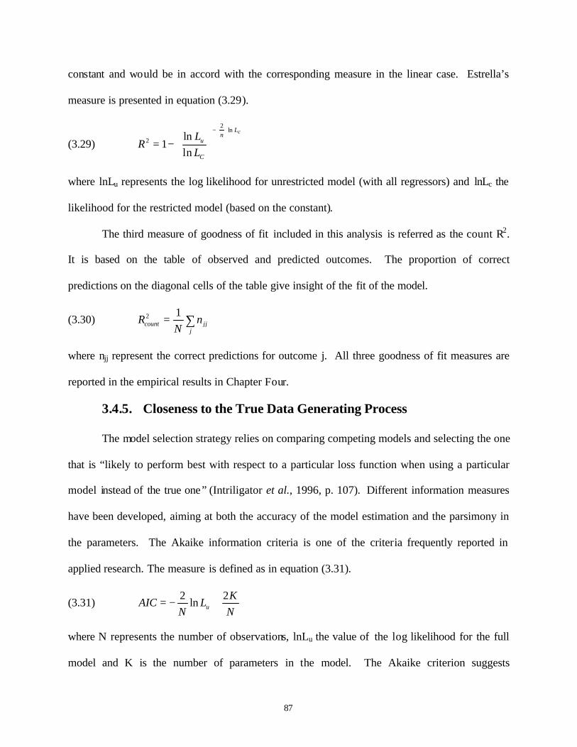
87
constant and would be in accord with the corresponding measure in the linear case. Estrella’s
measure is presented in equation (3.29).
(3.29)
2ln
2 ln1
ln
cLn
u
C
LR
L
−
= −
where lnLu represents the log likelihood for unrestricted model (with all regressors) and lnLc the
likelihood for the restricted model (based on the constant).
The third measure of goodness of fit included in this analysis is referred as the count R2.
It is based on the table of observed and predicted outcomes. The proportion of correct
predictions on the diagonal cells of the table give insight of the fit of the model.
(3.30) 2 1count jj
jR n
N= ∑
where njj represent the correct predictions for outcome j. All three goodness of fit measures are
reported in the empirical results in Chapter Four.
3.4.5. Closeness to the True Data Generating Process
The model selection strategy relies on comparing competing models and selecting the one
that is “likely to perform best with respect to a particular loss function when using a particular
model instead of the true one” (Intriligator et al., 1996, p. 107). Different information measures
have been developed, aiming at both the accuracy of the model estimation and the parsimony in
the parameters. The Akaike information criteria is one of the criteria frequently reported in
applied research. The measure is defined as in equation (3.31).
(3.31) 2 2
ln u
KAIC L
N N= − +
where N represents the number of observations, lnLu the value of the log likelihood for the full
model and K is the number of parameters in the model. The Akaike criterion suggests
88
maximizing the likelihood functions for each alternative function and selecting the model with
the smallest AIC value. The Schwartz criterion, on the other hand, is formulated as:
(3.32) 1
ln ln( )2uSC L K N= −
where N, K and lnLu receive the same specification as in the Akaike measure. The Schwartz
criterion places greater penalty on the dimension of the model and gives preference to the less
complex or parsimonious model. The decision rule is to select the model with the largest SC
numerical value. Both information measures were reported and discussed in the empirical
analysis.
3.4.6. LR Test for Joint Restrictions
Insight into the statistical significance of a particular estimated coefficient can be
obtained using the usual t-test. The test examines the significance of the hypothetical
assumption that a specific jβ is equal to zero (H0) against the alternative that it is not, and
determines the ratio of the particular estimate to the value of its standard error.
(3.33)
0
( ) 0
: 0
: 0
ˆ under
ˆ( )
j
A j
jN K
j
H
H
t Hse
T
β
β
β
β−
=
≠
= →
where ß̂ j and ˆsec(ß )j account for the value and the standard errors of the estimate of jβ ,
respectively, and N and K for the sample size and the number of explanatory variables included
in the model. The decision rule is that one should reject the null hypothesis when the absolute
value of the t statistic is greater than the critical value obtained from the t-distribution with N-K
degrees of freedom. Alternatively, a p-value associated with the t-statistic smaller than the 5
percent level of significance will imply the same conclusion.
89
The act of scaling down the number of variables from PCA necessitates the assumption
that many of the variables are zero and can be omitted in the probit and multivariate probit
analyses. Such linear restrictions on a set of coefficients require more elaborate tests than the
one discussed in the previous section. The likelihood ratio (LR) test constitutes one of the three
different tests based on the likelihood principle, which are used to analyze joint tests on the
parameters .β The Wald test is based solely on the unconstrained model and the Lagrange
Multiplier (LM) test on the restricted model. The LR test requires both constrained and
unconstrained models. All three tests would be asymptotically equivalent under the null
hypothesis that the restrictions hold.
The LR test was conducted to determine whether to reduce the number of explanatory
variables in the bivariate and multivariate probit model. The test is specified as:
(3.34)
0
2( ) 0
: ( ) 0 => the constrained model is appropriate: ( ) 0 => at least one of the coefficients is non zero
2 ln under
A
aR
Ju
H RH R
LR H
θθ
χλλ
=
≠
= − →
where ( )R θ accounts for the joint restrictions, λR and λu the log likelihood values for the
restricted and unrestricted models respectively, and J the number of restrictions. The decision
rule infers that one should fail to reject the null hypothesis that the complex restrictions hold
when the value of the LR statistic is smaller than the critical value of the 2χ distribution with J
degrees of freedom. Alternatively, a p-value associated with the LR statistic larger than the 5
percent level of significance would imply the same conclusion. Thus, one can conclude that the
parsimonious model is more appropriate.
90
3.4.7. Delta Method
The delta method is a means to determine the asymptotic distribution of a function of the
b coefficients, say g(b). The method specified in (3.35) allows for determining the asymptotic
variance of g(b) and deriving the standard errors required in the assessment of the statistical
significance of the function estimates.
(3.35) a
( )If then Est. Asy. Var[g(b)] * * '
'
and g(b) [ ( ), * * ']
gG G V G
N g G V G
ββ
β
∂= =
∂
→
where g(b) is the consistent estimator of ( )g β , G is the (J x K) Jacobian matrix of ( )g β with
respect to 'β and V the variance of the estimates b. The delta method was used in determining
the significance of the marginal effects obtained in the analysis.
3.5. Steps in the Empirical Analysis
In summary, the steps in the analysis are to:
1. Conduct descriptive statistics analysis;
2. Test for multicollinearity;
3. Conduct pincipal component analysis;
4. Conduct probit analysis on each specific best management practice with emphasis
on the heteroskedasticity test, goodness of fit, and marginal effects;
5. Select the appropriate model for each BMP to include in the multivariate probit
analysis based on the likelihood ratio test;
6. Conduct bivariate probit analyses based on the selected models from previous
steps, while stressing the contemporaneous correlation among the error terms, the
assumption of homoskedastic errors, and the marginal effects analysis; and

91
7. Conduct multivariate probit analyses that involve systems of three or more
management practices along with the assessment of discrete changes in the
probability as an alternative to estimation of marginal effects.
The empirical results from the analysis are presented in the next chapter. Discussion of the
results are also provided.
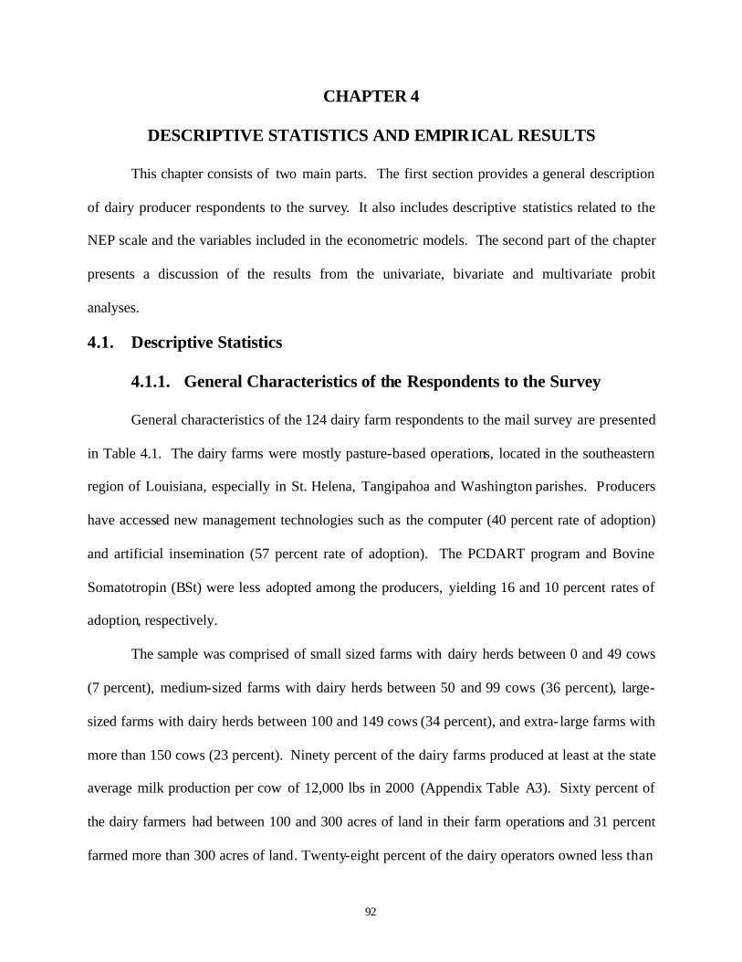
92
CHAPTER 4
DESCRIPTIVE STATISTICS AND EMPIRICAL RESULTS
This chapter consists of two main parts. The first section provides a general description
of dairy producer respondents to the survey. It also includes descriptive statistics related to the
NEP scale and the variables included in the econometric models. The second part of the chapter
presents a discussion of the results from the univariate, bivariate and multivariate probit
analyses.
4.1. Descriptive Statistics
4.1.1. General Characteristics of the Respondents to the Survey
General characteristics of the 124 dairy farm respondents to the mail survey are presented
in Table 4.1. The dairy farms were mostly pasture-based operations, located in the southeastern
region of Louisiana, especially in St. Helena, Tangipahoa and Washington parishes. Producers
have accessed new management technologies such as the computer (40 percent rate of adoption)
and artificial insemination (57 percent rate of adoption). The PCDART program and Bovine
Somatotropin (BSt) were less adopted among the producers, yielding 16 and 10 percent rates of
adoption, respectively.
The sample was comprised of small sized farms with dairy herds between 0 and 49 cows
(7 percent), medium-sized farms with dairy herds between 50 and 99 cows (36 percent), large-
sized farms with dairy herds between 100 and 149 cows (34 percent), and extra- large farms with
more than 150 cows (23 percent). Ninety percent of the dairy farms produced at least at the state
average milk production per cow of 12,000 lbs in 2000 (Appendix Table A3). Sixty percent of
the dairy farmers had between 100 and 300 acres of land in their farm operations and 31 percent
farmed more than 300 acres of land. Twenty-eight percent of the dairy operators owned less than
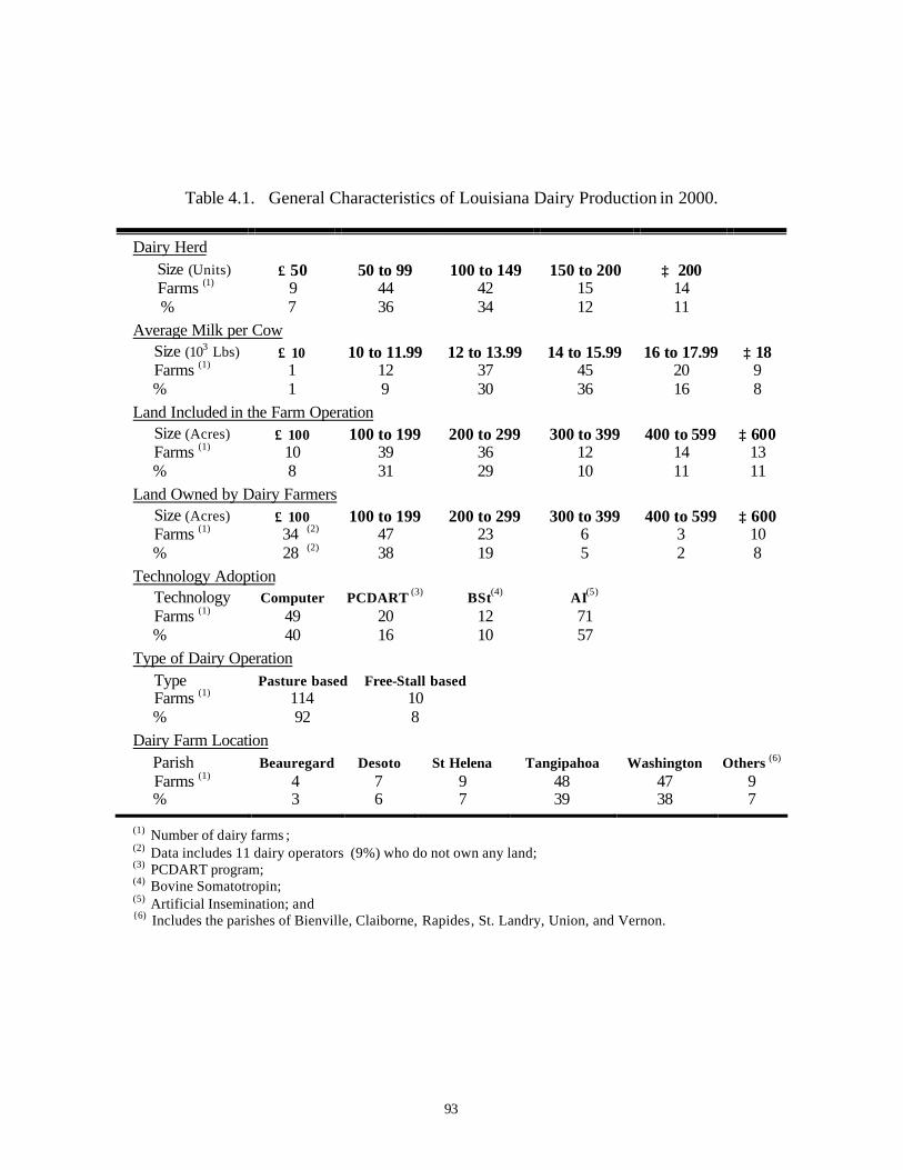
93
Table 4.1. General Characteristics of Louisiana Dairy Production in 2000.
Dairy Herd Size (Units) ≤ 50 50 to 99 100 to 149 150 to 200 ≥ 200 Farms (1) 9 44 42 15 14 % 7 36 34 12 11 Average Milk per Cow Size (103 Lbs) ≤ 10 10 to 11.99 12 to 13.99 14 to 15.99 16 to 17.99 ≥ 18 Farms (1) 1 12 37 45 20 9 % 1 9 30 36 16 8 Land Included in the Farm Operation Size (Acres) ≤ 100 100 to 199 200 to 299 300 to 399 400 to 599 ≥ 600 Farms (1) 10 39 36 12 14 13 % 8 31 29 10 11 11 Land Owned by Dairy Farmers Size (Acres) ≤ 100 100 to 199 200 to 299 300 to 399 400 to 599 ≥ 600 Farms (1) 34 (2) 47 23 6 3 10 % 28 (2) 38 19 5 2 8 Technology Adoption Technology Computer PCDART (3) BSt(4) AI(5) Farms (1) 49 20 12 71 % 40 16 10 57 Type of Dairy Operation Type Pasture based Free-Stall based Farms (1) 114 10 % 92 8 Dairy Farm Location Parish Beauregard Desoto St Helena Tangipahoa Washington Others (6) Farms (1) 4 7 9 48 47 9 % 3 6 7 39 38 7
(1) Number of dairy farms ; (2) Data includes 11 dairy operators (9%) who do not own any land; (3) PCDART program; (4) Bovine Somatotropin; (5) Artificial Insemination; and {6) Includes the parishes of Bienville, Claiborne, Rapides, St. Landry, Union, and Vernon.
94
100 acres of the farmland, 57 percent owned between 100 and 300 acres, and 15 percent owned
more than 300 acres.
As described in Table 4.2, the survey respondents were mostly male, between 40 and 59
years old, with a high school diploma or a bachelor’s degree. Eighty percent of the producers
had more than 10 years of experience in dairy farming. The majority of the producers did not
hold an off- farm job, but held membership in a milk cooperative.
More than half of the respondents were not aware of the Coastal Nonpoint Control
Program (CNCP) nor the effort to control water pollution through the Clean Water Act, as shown
in Table 4.3. Forty-eight percent of the producers had heard about BMPs for dairy operations.
The producers received information about water quality problems and BMPs primarily from the
Louisiana Cooperative Extension Service (LCES), government agencies and farm organizations
such as the Farm Bureau. Thirty-five percent of the dairy farms had developed and/or updated a
plan with NRCS within the last three years and 52 percent of the producers participated in a cost-
sharing program for implementing BMPs.
4.1.2. New Environmental Paradigm Scale
A summary of the distribution of the dairy producers’ responses to the NEP statements is
presented in Table 4.4. As discussed in the previous chapters, agreement with the eight odd-
numbered statements and disagreement with the seven even-numbered items indicate a pro-
environmental view. The frequency distribution of the responses shows that more than 50
percent of the dairy producers hold a pro-environmental view regarding statements 2, 3, 5, 7, 8,
9, 11, 13, and 14. Particularly, more than 60 percent of the producers agree with the views in
statements 3, 5, 9, and 13 which stipulate the disastrous consequences of human interference
with nature, severe human abuse of the environment, humans being subject to the laws of nature,
95
Table 4.2. Characteristics of Dairy Operators in 2000.
Gender Answers Male Female Number 112 12 % 90 10 Age Years ≤ 30 30 to 39 40 to 49 50 to 59 60 to 69 ≥ 70 Number 7 14 37 46 14 6 % 6 11 30 37 11 5 Experience in the Dairy Operation Years ≤ 10 10 to 19 20 to 29 30 to 39 ≥ 40 Number 25 29 38 24 8 % 20 24 31 19 6 Educational Attainment Degree NHS (1) High School Technical Bachelor Master Doctoral Number 12 70 10 26 6 0 % 10 56 8 21 5 0 Current Generation Operating the Dairy Farm Level 1st 2nd 3rd 4th 5th 6th Number 39 50 26 4 4 1 % 32 40 21 3 3 1 Off-Farm Job Answers Yes No Number 27 97 % 22 78 Membership in a Milk Cooperative Answers Yes No Number 104 20 % 84 16 Membership in the Dairy Herd Improvement Association Label Yes No Number 59 65 % 48 52
(1) No High School Diploma.
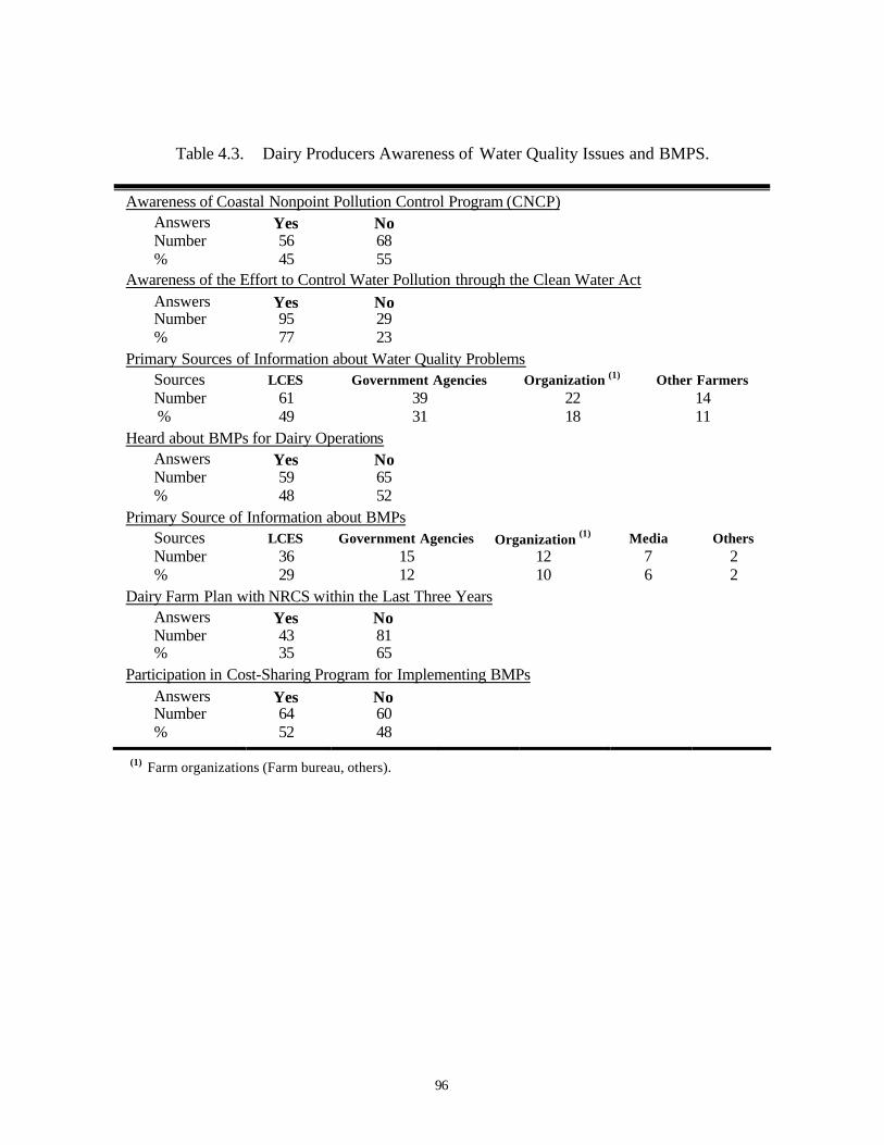
96
Table 4.3. Dairy Producers Awareness of Water Quality Issues and BMPS.
Awareness of Coastal Nonpoint Pollution Control Program (CNCP) Answers Yes No Number 56 68 % 45 55 Awareness of the Effort to Control Water Pollution through the Clean Water Act Answers Yes No Number 95 29 % 77 23 Primary Sources of Information about Water Quality Problems Sources LCES Government Agencies Organization (1) Other Farmers Number 61 39 22 14 % 49 31 18 11 Heard about BMPs for Dairy Operations Answers Yes No Number 59 65 % 48 52 Primary Source of Information about BMPs Sources LCES Government Agencies Organization (1) Media Others Number 36 15 12 7 2 % 29 12 10 6 2 Dairy Farm Plan with NRCS within the Last Three Years Answers Yes No Number 43 81 % 35 65 Participation in Cost-Sharing Program for Implementing BMPs Answers Yes No Number 64 60 % 52 48
(1) Farm organizations (Farm bureau, others).
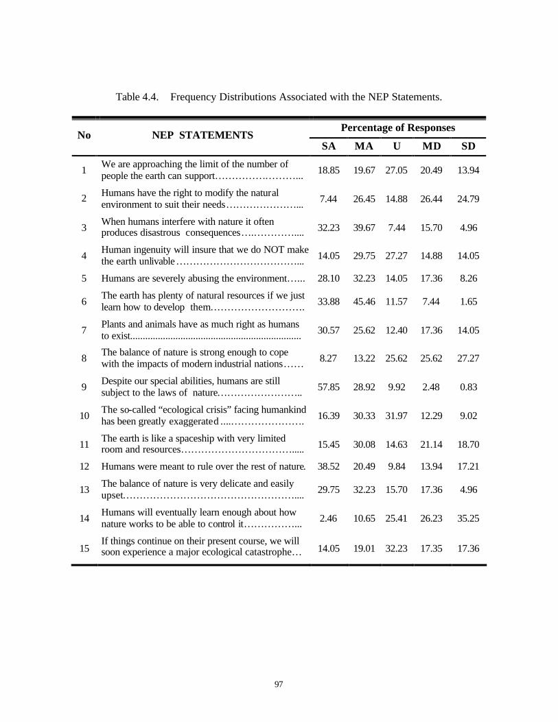
97
Table 4.4. Frequency Distributions Associated with the NEP Statements.
Percentage of Responses No NEP STATEMENTS
SA MA U MD SD
1 We are approaching the limit of the number of people the earth can support……………………... 18.85 19.67 27.05 20.49 13.94
2 Humans have the right to modify the natural environment to suit their needs…………………... 7.44 26.45 14.88 26.44 24.79
3 When humans interfere with nature it often produces disastrous consequences….………….... 32.23 39.67 7.44 15.70 4.96
4 Human ingenuity will insure that we do NOT make the earth unlivable………………………………... 14.05 29.75 27.27 14.88 14.05
5 Humans are severely abusing the environment…... 28.10 32.23 14.05 17.36 8.26
6 The earth has plenty of natural resources if we just learn how to develop them………………………. 33.88 45.46 11.57 7.44 1.65
7 Plants and animals have as much right as humans to exist.................................................................... 30.57 25.62 12.40 17.36 14.05
8 The balance of nature is strong enough to cope with the impacts of modern industrial nations…… 8.27 13.22 25.62 25.62 27.27
9 Despite our special abilities, humans are still subject to the laws of nature…………………….. 57.85 28.92 9.92 2.48 0.83
10 The so-called “ecological crisis” facing humankind has been greatly exaggerated ....…………………. 16.39 30.33 31.97 12.29 9.02
11 The earth is like a spaceship with very limited room and resources……………………………..... 15.45 30.08 14.63 21.14 18.70
12 Humans were meant to rule over the rest of nature. 38.52 20.49 9.84 13.94 17.21
13 The balance of nature is very delicate and easily upset…………………………………………….... 29.75 32.23 15.70 17.36 4.96
14 Humans will eventually learn enough about how nature works to be able to control it……………... 2.46 10.65 25.41 26.23 35.25
15 If things continue on their present course, we will soon experience a major ecological catastrophe… 14.05 19.01 32.23 17.35 17.36
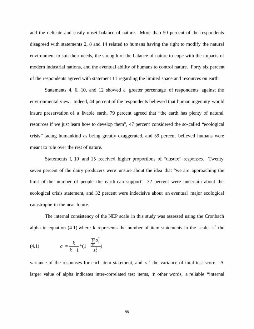
98
and the delicate and easily upset balance of nature. More than 50 percent of the respondents
disagreed with statements 2, 8 and 14 related to humans having the right to modify the natural
environment to suit their needs, the strength of the balance of nature to cope with the impacts of
modern industrial nations, and the eventual ability of humans to control nature. Forty six percent
of the respondents agreed with statement 11 regarding the limited space and resources on earth.
Statements 4, 6, 10, and 12 showed a greater percentage of respondents against the
environmental view. Indeed, 44 percent of the respondents believed that human ingenuity would
insure preservation of a livable earth, 79 percent agreed that “the earth has plenty of natural
resources if we just learn how to develop them”, 47 percent considered the so-called “ecological
crisis” facing humankind as being greatly exaggerated, and 59 percent believed humans were
meant to rule over the rest of nature.
Statements 1, 10 and 15 received higher proportions of “unsure” responses. Twenty
seven percent of the dairy producers were unsure about the idea that “we are approaching the
limit of the number of people the earth can support”, 32 percent were uncertain about the
ecological crisis statement, and 32 percent were indecisive about an eventual major ecological
catastrophe in the near future.
The internal consistency of the NEP scale in this study was assessed using the Cronbach
alpha in equation (4.1) where k represents the number of item statements in the scale, si2 the
(4.1)
2
2*(1 )
1
ik
T
sk
k sα = −
−
∑
variance of the responses for each item statement, and sT2 the variance of total test score. A
larger value of alpha indicates inter-correlated test items, in other words, a reliable “internal
99
consistency” of the scale measure (Mueller, 1986; Nunnally and Bernstein, 1994). A coefficient
alpha of 0.78 was found. This result indicates reasonable internal consistency of the scale.
4.1.3. Adoption Rates of BMPs
Different rates of adoption were found for each BMP as displayed in Table 4.5.
Adoption rates vary across BMP mainly due to a need of greater information or the non
applicability of the specific practice to the farm.
Erosion and sediment control practices. Conservation tillage practices had the highest
rate of adoption among the management practices targeting the control of soil erosion and
sediment transport. Seventy-seven percent of the dairy producers had adopted a tillage practice
system to maintain crop residues near soil surfaces. Riparian forest buffers and streambank and
shoreline protection were the least adopted in the group, with only 28 percent adoption rates for
either practice. The low adoption rates of streambank protection could be because of the few
farms having a stream and/or river running through. The survey responses show that 25 percent
of the dairy farms had a stream and/or river running through their farm land. The remaining
dairy producers had a stream and/or river less than half a mile away from the farm (5 percent),
between one half to one mile away from the farm (21 percent), and more than one mile away
from the farm (49 percent).
The adoption rates of filter strips and heavy use area protection were 35 and 31 percent,
respectively. These results suggest limited establishment of vegetative areas to trap sediment
and other pollutants from runoff and wastewater, and/or appropriate surfacing covers to protect
frequent ly and intensively used areas. Grassed waterways and sediment basin management
practices had adoption rates of 43 percent. Thus, 43 percent of the respondents had established
constructed channels with suitable vegetation to stabilize the conveyance of runoff from water
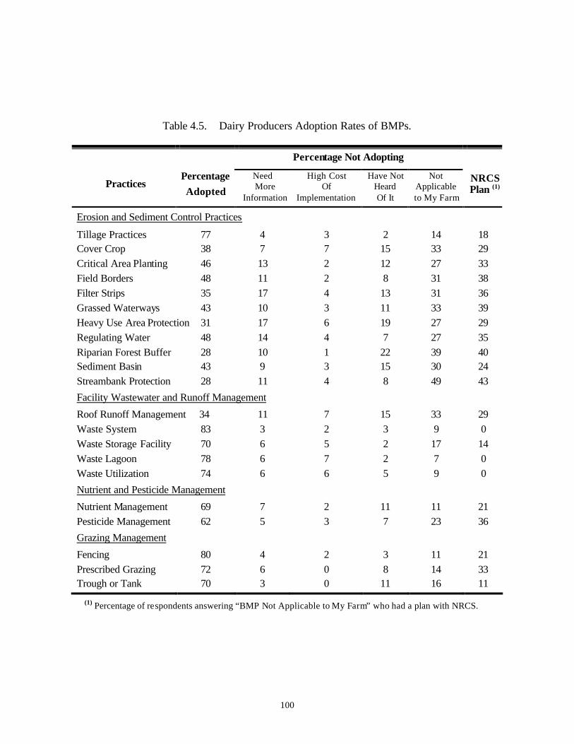
100
Table 4.5. Dairy Producers Adoption Rates of BMPs.
Percentage Not Adopting
Practices
Percentage Adopted
Need More
Information
High Cost Of
Implementation
Have Not Heard Of It
Not Applicable to My Farm
NRCS Plan (1)
Erosion and Sediment Control Practices
Tillage Practices 77 4 3 2 14 18 Cover Crop 38 7 7 15 33 29 Critical Area Planting 46 13 2 12 27 33 Field Borders 48 11 2 8 31 38 Filter Strips 35 17 4 13 31 36 Grassed Waterways 43 10 3 11 33 39 Heavy Use Area Protection 31 17 6 19 27 29 Regulating Water 48 14 4 7 27 35 Riparian Forest Buffer 28 10 1 22 39 40 Sediment Basin 43 9 3 15 30 24 Streambank Protection 28 11 4 8 49 43
Facility Wastewater and Runoff Management
Roof Runoff Management 34 11 7 15 33 29 Waste System 83 3 2 3 9 0 Waste Storage Facility 70 6 5 2 17 14 Waste Lagoon 78 6 7 2 7 0 Waste Utilization 74 6 6 5 9 0
Nutrient and Pesticide Management
Nutrient Management 69 7 2 11 11 21 Pesticide Management 62 5 3 7 23 36
Grazing Management
Fencing 80 4 2 3 11 21 Prescribed Grazing 72 6 0 8 14 33 Trough or Tank 70 3 0 11 16 11
(1) Percentage of respondents answering “BMP Not Applicable to My Farm” who had a plan with NRCS.
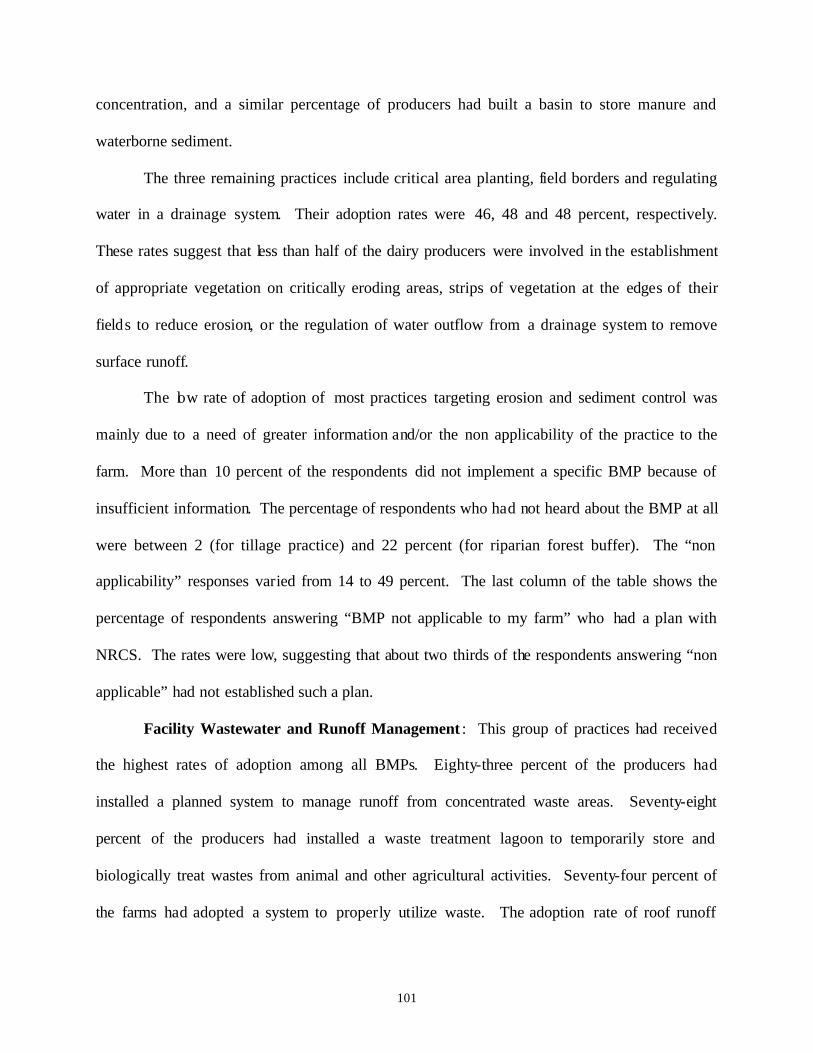
101
concentration, and a similar percentage of producers had built a basin to store manure and
waterborne sediment.
The three remaining practices include critical area planting, field borders and regulating
water in a drainage system. Their adoption rates were 46, 48 and 48 percent, respectively.
These rates suggest that less than half of the dairy producers were involved in the establishment
of appropriate vegetation on critically eroding areas, strips of vegetation at the edges of their
fields to reduce erosion, or the regulation of water outflow from a drainage system to remove
surface runoff.
The low rate of adoption of most practices targeting erosion and sediment control was
mainly due to a need of greater information and/or the non applicability of the practice to the
farm. More than 10 percent of the respondents did not implement a specific BMP because of
insufficient information. The percentage of respondents who had not heard about the BMP at all
were between 2 (for tillage practice) and 22 percent (for riparian forest buffer). The “non
applicability” responses varied from 14 to 49 percent. The last column of the table shows the
percentage of respondents answering “BMP not applicable to my farm” who had a plan with
NRCS. The rates were low, suggesting that about two thirds of the respondents answering “non
applicable” had not established such a plan.
Facility Wastewater and Runoff Management : This group of practices had received
the highest rates of adoption among all BMPs. Eighty-three percent of the producers had
installed a planned system to manage runoff from concentrated waste areas. Seventy-eight
percent of the producers had installed a waste treatment lagoon to temporarily store and
biologically treat wastes from animal and other agricultural activities. Seventy-four percent of
the farms had adopted a system to properly utilize waste. The adoption rate of roof runoff
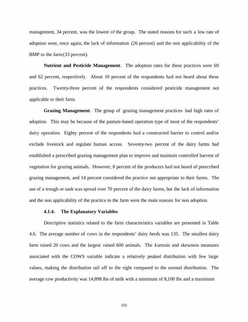
102
management, 34 percent, was the lowest of the group. The stated reasons for such a low rate of
adoption were, once again, the lack of information (26 percent) and the non applicability of the
BMP to the farm (33 percent).
Nutrient and Pesticide Management. The adoption rates for these practices were 69
and 62 percent, respectively. About 10 percent of the respondents had not heard about these
practices. Twenty-three percent of the respondents considered pesticide management not
applicable to their farm.
Grazing Management. The group of grazing management practices had high rates of
adoption. This may be because of the pasture-based operation type of most of the respondents’
dairy operation. Eighty percent of the respondents had a constructed barrier to control and/or
exclude livestock and regulate human access. Seventy-two percent of the dairy farms had
established a prescribed grazing management plan to improve and maintain controlled harvest of
vegetation for grazing animals. However, 8 percent of the producers had not heard of prescribed
grazing management, and 14 percent considered the practice not appropriate to their farms. The
use of a trough or tank was spread over 70 percent of the dairy farms, but the lack of information
and the non applicability of the practice to the farm were the main reasons for non adoption.
4.1.4. The Explanatory Variables
Descriptive statistics related to the farm characteristics variables are presented in Table
4.6. The average number of cows in the respondents’ dairy herds was 135. The smallest dairy
farm raised 20 cows and the largest raised 600 animals. The kurtosis and skewness measures
associated with the COWS variable indicate a relatively peaked distribution with few large
values, making the distribution tail off to the right compared to the normal distribution. The
average cow productivity was 14,898 lbs of milk with a minimum of 8,100 lbs and a maximum
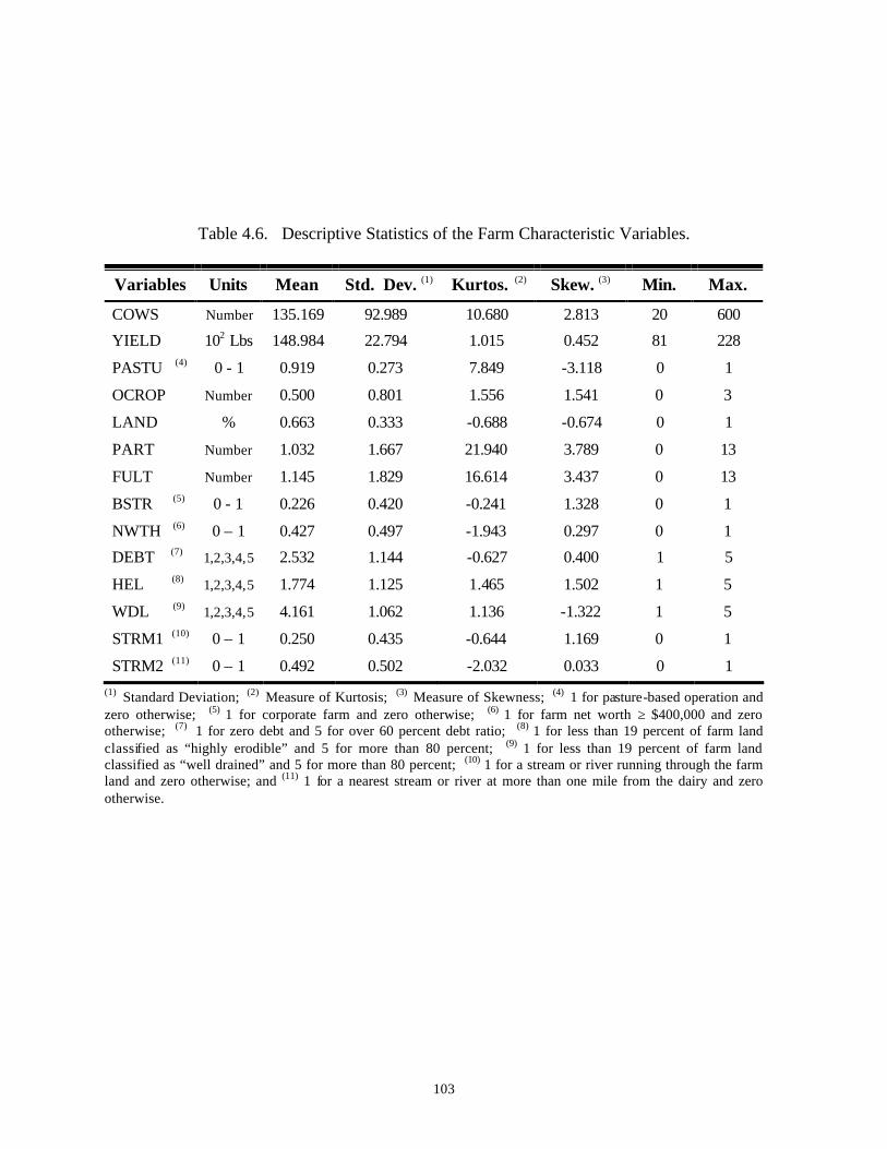
103
Table 4.6. Descriptive Statistics of the Farm Characteristic Variables.
Variables Units Mean Std. Dev. (1) Kurtos. (2) Skew. (3) Min. Max.
COWS Number 135.169 92.989 10.680 2.813 20 600
YIELD 102 Lbs 148.984 22.794 1.015 0.452 81 228
PASTU (4) 0 - 1 0.919 0.273 7.849 -3.118 0 1
OCROP Number 0.500 0.801 1.556 1.541 0 3
LAND % 0.663 0.333 -0.688 -0.674 0 1
PART Number 1.032 1.667 21.940 3.789 0 13
FULT Number 1.145 1.829 16.614 3.437 0 13
BSTR (5) 0 - 1 0.226 0.420 -0.241 1.328 0 1
NWTH (6) 0 – 1 0.427 0.497 -1.943 0.297 0 1
DEBT (7) 1,2,3,4,5 2.532 1.144 -0.627 0.400 1 5
HEL (8) 1,2,3,4,5 1.774 1.125 1.465 1.502 1 5
WDL (9) 1,2,3,4,5 4.161 1.062 1.136 -1.322 1 5
STRM1 (10) 0 – 1 0.250 0.435 -0.644 1.169 0 1
STRM2 (11) 0 – 1 0.492 0.502 -2.032 0.033 0 1 (1) Standard Deviation; (2) Measure of Kurtosis; (3) Measure of Skewness; (4) 1 for pasture-based operation and zero otherwise; (5) 1 for corporate farm and zero otherwise; (6) 1 for farm net worth ≥ $400,000 and zero otherwise; (7) 1 for zero debt and 5 for over 60 percent debt ratio; (8) 1 for less than 19 percent of farm land classified as “highly erodible” and 5 for more than 80 percent; (9) 1 for less than 19 percent of farm land classified as “well drained” and 5 for more than 80 percent; (10) 1 for a stream or river running through the farm land and zero otherwise; and (11) 1 for a nearest stream or river at more than one mile from the dairy and zero otherwise.
104
of 22,800 lbs. Variable YIELD was scaled down by 100 for the regression analyses, to reduce
the size difference between explanatory variables. Variable PASTU yielded a mean value of
0.92 and a standard deviation of 0.27. The negative skewness value indicates the relatively small
number of farms associated with PASTU values equal to zero. This is consistent with the fact
that 92 percent of the dairy farms were pasture-based operations. Most of the dairy farms were
not diversified with the exception of a few farms. The percentage of respondents who raised
corn, cotton, wheat, soybean, oats, broilers, or beef were, respectively, 19, 1, 2, 4, 8, 2, and 14.
Nineteen percent of the respondents were involved in forestry. The average number of other
enterprises was 0.5 with a minimum of zero and a maximum of 3 enterprises. The distribution of
the OCROP variable is slightly peaked and tailed to the right compared to the normal
distribution.
The mean proportion of land owned to total acres of land included in the farm operation
was 66 percent with a standard deviation of 33 percent. The distribution of the LAND variable
is slightly flat and tailed off to the left compared to the normal distribution. The number of part-
time workers varied from zero to 13, with a mean value of 1.03 and a standard deviation of 1.67.
The large kurtosis measure indicates a relatively peaked distribution of variable PART compared
to the normal distribution. Similar results were obtained with the number of fulltime workers.
Variable BSTR was included as a dummy variable that takes the value of 1 if the dairy
farm is structured as a corporation. The mean value of 0.23 confirms the fact that 23 percent of
the respondents operated a family or non-family corporation farm. Variable NWTH was
incorporated as a dummy variable with a value of 1 for farm net worth greater than or equal to
$400,000. The mean value was 0.43 with a standard deviation of 0.5.
105
Debt to asset ratio was coded as 1, 2, 3, 4, and 5 for values of zero, 1 to 20 percent, 21 to
40 percent, 41 to 60 percent and over 60 percent, respectively. The variable was treated as
continuous. Results from the survey indicated that 20 percent of the respondents were debt- free,
33 percent had 1 to 20 percent debt/asset ratios, 26 percent had 21 to 40 percent, 15 percent had
41 to 60 percent and 5 percent had over 60 percent. The DEBT variable has a mean value of 2.5
and a slightly flat distribution, tailed off to the right relative to the normal distribution.
The highly erodible land variable (HEL), also treated as continuous, took the values of 1,
2, 3, 4, and 5 if the percentage of respondents’ land fell into the following categories: 0 to 19
percent, 20 to 39 percent, 40 to 59 percent, 60 to 79 percent, or 80 to 100 percent, respectively.
Fifty-seven percent of the respondents had less than 20 percent highly erodible land, 23 percent
had 20 to 39 percent, 10 percent had 40 to 59 percent, 5 percent had 60 to 79 percent and 5
percent had 80 to 100 percent. The well-drained land variable (WDL) was included as
continuous similar to variable HEL. Results show that half of the respondents did not experience
major land drainage problems. Only 3 percent of the respondents had less than 20 percent well-
drained land, 6 percent had 20 to 39 percent, 10 percent had 40 to 59 percent, 31 percent had 60
to 79 percent, and 49 percent had 80 to 100 percent. Variable WDL has a mean value of 4.16
and a standard deviation of 1.06.
The existence of a stream and/or river on the dairy farm or nearby was accounted for
using two dummy variables: STRM1 accounts for a stream or river running through the farm,
and STRM2 for the nearest stream or river distant from the farm. Twenty-five percent of the
respondents had a stream and/or river running through their farmland. Among the remaining
producers who did not have a stream on their farm, 5 percent were half a mile away, 21 percent
106
were between one-half and one mile, and 49 percent were more than one mile away from the
nearest stream.
Variables that account for farm characteristics are described in Table 4.7. Respondents to
the mail survey were, on average, 51 years old. The youngest producer was 26 and the oldest 78
years old. Twenty-six percent of the respondents had a college degree, 22 percent had an off-
farm job, 26 percent had family who planned to take over the operation upon the operator’s
retirement, and 52 percent participated in a cost sharing program.
Respondents’ years of experience in dairy farming were between 2 to 50 years, yielding
an average of 23 years. Specifically, 11 percent of the respondents had less than 5 years of
experience, 9 percent had 6 to 9 years, 24 percent had 10 to 19 years, 31 percent had 20 to 29
years, 19 percent had 30 to 39 years, and 6 percent had more than 40 years of experience.
Variable EXP has a slightly flat and positively skewed distribution.
Descriptive statistics related to the institutional variables are presented in Table 4.8.
Eighty-four percent of the respondents held membership in a milk cooperative and 48 percent in
the DHIA. Thirty-five percent of the respondents had developed a dairy farm plan with NRCS.
The average number of meetings with LCES over the year 2000 was 2.5, with a minimum of
zero and a maximum of six meetings. Twenty-six of the respondents did not attend any meetings
with LCES in 2000, 38 percent attended 1 or 2, 23 percent attended 3 to 4, and 12 percent
attended 4 to 6 meetings. Variable LCES has a relatively flat distribution, tailed off to the right.
Survey responses show that respondents attended, on average, 2 to 3 seminars and/or
meetings that dealt with dairy industry issues in 2000, with a maximum of 20 meetings attended.
The attendance was as follows: 31 percent of the producers did not attend any meetings at all, 60
percent attended less than 5 meetings, 6 percent participated in 5 to 10, and 3 percent attended
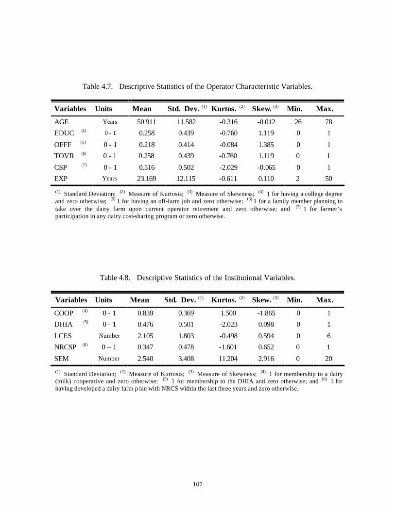
107
Table 4.7. Descriptive Statistics of the Operator Characteristic Variables.
Variables Units Mean Std. Dev. (1) Kurtos. (2) Skew. (3) Min. Max.
AGE Years 50.911 11.582 -0.316 -0.012 26 78
EDUC (4) 0 - 1 0.258 0.439 -0.760 1.119 0 1
OFFF (5) 0 - 1 0.218 0.414 -0.084 1.385 0 1
TOVR (6) 0 - 1 0.258 0.439 -0.760 1.119 0 1
CSP (7) 0 - 1 0.516 0.502 -2.029 -0.065 0 1
EXP Years 23.169 12.115 -0.611 0.110 2 50
(1) Standard Deviation; (2) Measure of Kurtosis; (3) Measure of Skewness; (4) 1 for having a college degree and zero otherwise; (5) 1 for having an off-farm job and zero otherwise; (6) 1 for a family member planning to take over the dairy farm upon current operator retirement and zero otherwise; and (7) 1 for farmer’s participation in any dairy cost-sharing program or zero otherwise.
Table 4.8. Descriptive Statistics of the Institutional Variables.
Variables Units Mean Std. Dev. (1) Kurtos. (2) Skew. (3) Min. Max.
COOP (4) 0 - 1 0.839 0.369 1.500 -1.865 0 1
DHIA (5) 0 - 1 0.476 0.501 -2.023 0.098 0 1
LCES Number 2.105 1.803 -0.498 0.594 0 6
NRCSP (6) 0 – 1 0.347 0.478 -1.601 0.652 0 1
SEM Number 2.540 3.408 11.204 2.916 0 20
(1) Standard Deviation; (2) Measure of Kurtosis; (3) Measure of Skewness; (4) 1 for membership to a dairy (milk) cooperative and zero otherwise; (5) 1 for membership to the DHIA and zero otherwise; and (6) 1 for having developed a dairy farm p lan with NRCS within the last three years and zero otherwise.
108
more than 10 meetings. Variable SEM has a relatively peaked distribution, tailed off to the right
because of the few large values.
Descriptive statistics related to the attitudinal variables are presented in Table 4.9.
Survey results show that 73 percent of the respondents tended to avoid risk whenever it was
possib le in their investment decisions, 19 percent neither sought nor avoided risk in their
investment decisions, and 8 percent tended to take on substantial levels of risk in their
investment decisions.
On average, respondents perceived their social relationships with the different entities
related to their farm operation as “somewhat important” to “very important”. Each of the five
social capital variables has a relatively peaked and negatively skewed distribution compared to
the normal distribution. Respondents’ average score related to the environmental variable was
3.22 with a standard deviation of 0.61. The lowest value of 1.53 suggest a more anthropocentric
view and the largest value of 4.53 indicate a strong pro-environmental attitude. Variable ENV
has a slightly peaked and negatively skewed distribution compared to the normal distribution.
4.2. Empirical Results
4.2.1. Test for Multicollinearity
Collinearity among the 32 variables hypothesized as important in determining producers’
decisions to adopt BMPs was analyzed using SAS. The collinearity diagnostic consisted of
determining the eigenvalues ( )iλ , condition indexes ( )iη and the proportion of variation matrix.
The procedure was to associate the lowest eigenvalues with condition index values of at least 30
to specific independent variables. A first test was run on the complete set of 32 explanatory
variables. Summary of the results, presented in Appendix Table C1, showed four values above
30 at the bottom of the condition indexes column. This suggested a strong collinearity problem
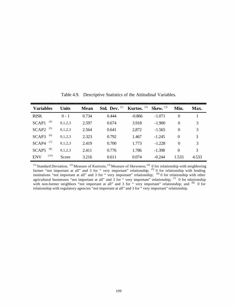
109
Table 4.9. Descriptive Statistics of the Attitudinal Variables.
Variables Units Mean Std. Dev. (1) Kurtos. (2) Skew. (3) Min. Max.
RISK 0 - 1 0.734 0.444 -0.866 -1.071 0 1
SCAP1 (4) 0,1,2,3 2.597 0.674 3.918 -1.900 0 3
SCAP2 (5) 0,1,2,3 2.564 0.641 2,872 -1.565 0 3
SCAP3 (6) 0,1,2,3 2.323 0.792 1.467 -1.245 0 3
SCAP4 (7) 0,1,2,3 2.419 0.700 1.773 -1.228 0 3
SCAP5 (8) 0,1,2,3 2.411 0.776 1.786 -1.398 0 3
ENV (10) Score 3.216 0.611 0.074 -0.244 1.533 4.533
(1) Standard Deviation; (2) Measure of Kurtosis; (3) Measure of Skewness; (4) 0 for relationship with neighboring farmer “not important at all” and 3 for “ very important” relationship; (5) 0 for relationship with lending institutions “not important at all” and 3 for “ very important” relationship; (6) 0 for relationship with other agricultural businesses “not important at all” and 3 for “ very important” relationship; (7) 0 for relationship with non-farmer neighbors “not important at all” and 3 for “ very important” relationship; and (8) 0 for relationship with regulatory agencies “not important at all” and 3 for “ very important” relationship.
110
between four variables. Variables YIELD, AGE, SCAP1 and SCAP3 were identified as strongly
correlated using the rule of thumb of 50 percent on the sum of the last four lines in each column
of the proportion variance matrix. Social relationships with neighboring farmers (SCAP1) as
well as other agricultural businesses (SCAP3) were assessed as less important in producers’
decisions to adopt and, therefore, were excluded from the set of explanatory variables to reduce
the collinearity problem.
A second test was performed using the 30 remaining variables and the results are
presented in appendix Table C2. Variables YIELD and AGE remained strongly correlated. The
process of discarding variables through principal components analysis constitutes another
method for dealing with the collinearity problem. Therefore, all 30 variables were included in
the base model for the probit analysis of each individual BMP, but their number was reduced for
multivariate probit analysis purposes using PCA.
4.2.2. Principal Component Analysis
Results of the PCA are presented in Appendix D. Two different levels of the eigenvalues
( )iλ were selected based on previous research. First, an optimum eigenvalue of 0.7, as
suggested by Jolliffe (1973) and Daultrey (1976), was considered in the process of discarding
variables for the parsimonious probit model for each BMP. The process allowed for the
retention of 17 variables. The need for further reduction of the number of independent variables
required the selection of a larger value of λ equal to 1. The PCA process allowed for the
retention of 12 variables necessary for the multivariable probit analyses.
4.2.3. Probit Analysis on Each Specific BMP
Four different models were estimated for each BMP. The base model included all 30
variables retained from the collinearity analysis. The second model incorporated the 17 variables
111
retained from PCA procedure. The third model was an extension of the second model and
included extra variables from the base model which were significant at the 10 percent level. The
fourth model included variables from the base model which were significant at the 50 percent
level. Results of the heteroskedasticity tests showed all Lagrange Multiplier (LM) statistic
values associated with very large p-values. Thus, one could conclude that the models were not
affected by heteroskedasticity.
The goodness of fit of each model was assessed using McFadden’s and Estrella’s R2
statistics. Most of the values were very low, about 0.20, except for the models associated with
conservation tillage practices (0.30), streambank protection (0.32), waste management system
(0.50), nutrient management (0.33), and prescribed grazing (0.40). AIC and SC criteria were
estimated to determine the model closeness to the data generation process.
The conduct of the likelihood ratio test allowed for selecting the relevant parsimonious
model to be included in the multivariate analysis. Marginal effects at mean values of all
variables as well as at selected values of the dummies were estimated. Finally, discrete changes
in the predicted probabilities were assessed for dummy variables with significant coefficients .β
The summary of results for the selected model associated with each BMP probit analysis is
presented in Table 4.10.
4.2.3.1. Erosion and Sediment Control Practices
The final model for conservation tillage practices included the 17 variables retained from
PCA. Seven variables were significant at the 5 or 10 percent level of significance. Variables
COWS, YIELD, OFFF, and LCES had the expected positive signs. The magnitude of the
marginal effects of COWS and YIELD variables on the probability that a dairy producer would
adopt conservation tillage practices were relatively small, about 0.002 and 0.008, respectively.
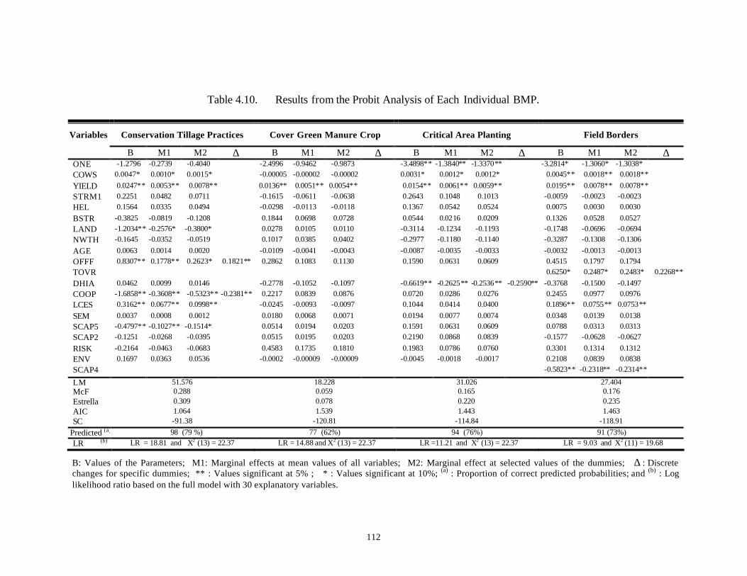
112
Table 4.10. Results from the Probit Analysis of Each Individual BMP.
Conservation Tillage Practices Cover Green Manure Crop Critical Area Planting Field Borders Variables
B M1 M2 ∆ B M1 M2 ∆ B M1 M2 ∆ B M1 M2 ∆ ONE -1.2796 -0.2739 -0.4040 -2.4996 -0.9462 -0.9873 -3.4898** -1.3840** -1.3370** -3.2814* -1.3060* -1.3038* COWS 0.0047* 0.0010* 0.0015* -0.00005 -0.00002 -0.00002 0.0031* 0.0012* 0.0012* 0.0045** 0.0018** 0.0018** YIELD 0.0247** 0.0053** 0.0078** 0.0136** 0.0051** 0.0054** 0.0154** 0.0061** 0.0059** 0.0195** 0.0078** 0.0078** STRM1 0.2251 0.0482 0.0711 -0.1615 -0.0611 -0.0638 0.2643 0.1048 0.1013 -0.0059 -0.0023 -0.0023 HEL 0.1564 0.0335 0.0494 -0.0298 -0.0113 -0.0118 0.1367 0.0542 0.0524 0.0075 0.0030 0.0030 BSTR -0.3825 -0.0819 -0.1208 0.1844 0.0698 0.0728 0.0544 0.0216 0.0209 0.1326 0.0528 0.0527 LAND -1.2034** -0.2576* -0.3800* 0.0278 0.0105 0.0110 -0.3114 -0.1234 -0.1193 -0.1748 -0.0696 -0.0694 NWTH -0.1645 -0.0352 -0.0519 0.1017 0.0385 0.0402 -0.2977 -0.1180 -0.1140 -0.3287 -0.1308 -0.1306 AGE 0.0063 0.0014 0.0020 -0.0109 -0.0041 -0.0043 -0.0087 -0.0035 -0.0033 -0.0032 -0.0013 -0.0013 OFFF 0.8307** 0.1778** 0.2623* 0.1821** 0.2862 0.1083 0.1130 0.1590 0.0631 0.0609 0.4515 0.1797 0.1794 TOVR 0.6250* 0.2487* 0.2483* 0.2268**
DHIA 0.0462 0.0099 0.0146 -0.2778 -0.1052 -0.1097 -0.6619** -0.2625** -0.2536** -0.2590** -0.3768 -0.1500 -0.1497 COOP -1.6858** -0.3608** -0.5323** -0.2381** 0.2217 0.0839 0.0876 0.0720 0.0286 0.0276 0.2455 0.0977 0.0976 LCES 0.3162** 0.0677** 0.0998** -0.0245 -0.0093 -0.0097 0.1044 0.0414 0.0400 0.1896** 0.0755** 0.0753** SEM 0.0037 0.0008 0.0012 0.0180 0.0068 0.0071 0.0194 0.0077 0.0074 0.0348 0.0139 0.0138 SCAP5 -0.4797** -0.1027** -0.1514* 0.0514 0.0194 0.0203 0.1591 0.0631 0.0609 0.0788 0.0313 0.0313 SCAP2 -0.1251 -0.0268 -0.0395 0.0515 0.0195 0.0203 0.2190 0.0868 0.0839 -0.1577 -0.0628 -0.0627 RISK -0.2164 -0.0463 -0.0683 0.4583 0.1735 0.1810 0.1983 0.0786 0.0760 0.3301 0.1314 0.1312 ENV 0.1697 0.0363 0.0536 -0.0002 -0.00009 -0.00009 -0.0045 -0.0018 -0.0017 0.2108 0.0839 0.0838 SCAP4 -0.5823** -0.2318** -0.2314** LM 51.576 18.228 31.026 27.404 McF 0.288 0.059 0.165 0.176 Estrella 0.309 0.078 0.220 0.235 AIC 1.064 1.539 1.443 1.463 SC -91.38 -120.81 -114.84 -118.91
Predicted (a) 98 (79 %) 77 (62%) 94 (76%) 91 (73%) LR (b) LR = 18.81 and X2 (13) = 22.37 LR = 14.88 and X2 (13) = 22.37 LR =11.21 and X2 (13) = 22.37 LR = 9.03 and X2 (11) = 19.68
B: Values of the Parameters; M1: Marginal effects at mean values of all variables; M2: Marginal effect at selected values of the dummies; ∆ : Discrete changes for specific dummies; ** : Values significant at 5% ; * : Values significant at 10%; (a) : Proportion of correct predicted probabilities; and (b) : Log likelihood ratio based on the full model with 30 explanatory variables.
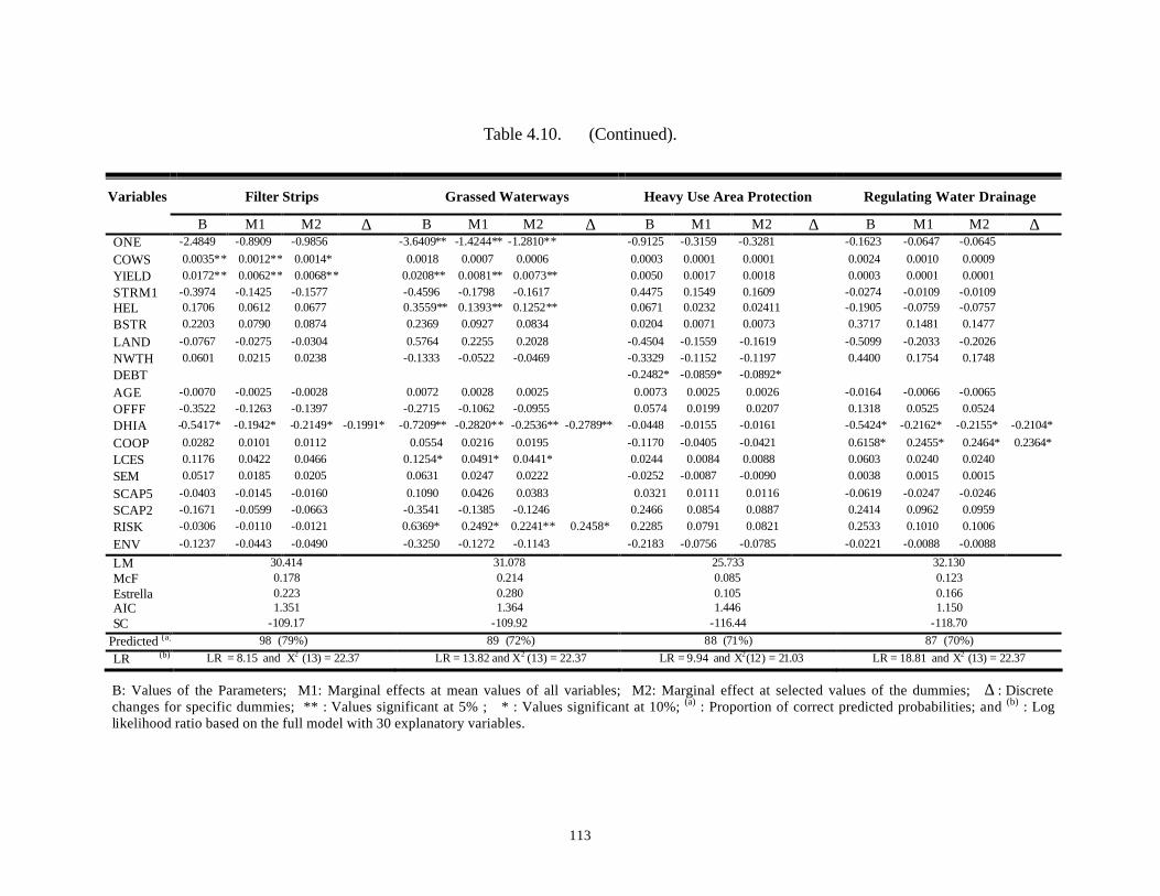
113
Table 4.10. (Continued).
Filter Strips Grassed Waterways Heavy Use Area Protection Regulating Water Drainage Variables
B M1 M2 ∆ B M1 M2 ∆ B M1 M2 ∆ B M1 M2 ∆ ONE -2.4849 -0.8909 -0.9856 -3.6409** -1.4244** -1.2810** -0.9125 -0.3159 -0.3281 -0.1623 -0.0647 -0.0645
COWS 0.0035** 0.0012** 0.0014* 0.0018 0.0007 0.0006 0.0003 0.0001 0.0001 0.0024 0.0010 0.0009 YIELD 0.0172** 0.0062** 0.0068** 0.0208** 0.0081** 0.0073** 0.0050 0.0017 0.0018 0.0003 0.0001 0.0001 STRM1 -0.3974 -0.1425 -0.1577 -0.4596 -0.1798 -0.1617 0.4475 0.1549 0.1609 -0.0274 -0.0109 -0.0109 HEL 0.1706 0.0612 0.0677 0.3559** 0.1393** 0.1252** 0.0671 0.0232 0.02411 -0.1905 -0.0759 -0.0757 BSTR 0.2203 0.0790 0.0874 0.2369 0.0927 0.0834 0.0204 0.0071 0.0073 0.3717 0.1481 0.1477
LAND -0.0767 -0.0275 -0.0304 0.5764 0.2255 0.2028 -0.4504 -0.1559 -0.1619 -0.5099 -0.2033 -0.2026 NWTH 0.0601 0.0215 0.0238 -0.1333 -0.0522 -0.0469 -0.3329 -0.1152 -0.1197 0.4400 0.1754 0.1748 DEBT -0.2482* -0.0859* -0.0892*
AGE -0.0070 -0.0025 -0.0028 0.0072 0.0028 0.0025 0.0073 0.0025 0.0026 -0.0164 -0.0066 -0.0065 OFFF -0.3522 -0.1263 -0.1397 -0.2715 -0.1062 -0.0955 0.0574 0.0199 0.0207 0.1318 0.0525 0.0524 DHIA -0.5417* -0.1942* -0.2149* -0.1991* -0.7209** -0.2820** -0.2536** -0.2789** -0.0448 -0.0155 -0.0161 -0.5424* -0.2162* -0.2155* -0.2104*
COOP 0.0282 0.0101 0.0112 0.0554 0.0216 0.0195 -0.1170 -0.0405 -0.0421 0.6158* 0.2455* 0.2464* 0.2364* LCES 0.1176 0.0422 0.0466 0.1254* 0.0491* 0.0441* 0.0244 0.0084 0.0088 0.0603 0.0240 0.0240 SEM 0.0517 0.0185 0.0205 0.0631 0.0247 0.0222 -0.0252 -0.0087 -0.0090 0.0038 0.0015 0.0015
SCAP5 -0.0403 -0.0145 -0.0160 0.1090 0.0426 0.0383 0.0321 0.0111 0.0116 -0.0619 -0.0247 -0.0246 SCAP2 -0.1671 -0.0599 -0.0663 -0.3541 -0.1385 -0.1246 0.2466 0.0854 0.0887 0.2414 0.0962 0.0959 RISK -0.0306 -0.0110 -0.0121 0.6369* 0.2492* 0.2241** 0.2458* 0.2285 0.0791 0.0821 0.2533 0.1010 0.1006
ENV -0.1237 -0.0443 -0.0490 -0.3250 -0.1272 -0.1143 -0.2183 -0.0756 -0.0785 -0.0221 -0.0088 -0.0088
LM 30.414 31.078 25.733 32.130 McF 0.178 0.214 0.085 0.123 Estrella 0.223 0.280 0.105 0.166 AIC 1.351 1.364 1.446 1.150 SC -109.17 -109.92 -116.44 -118.70
Predicted (a) 98 (79%) 89 (72%) 88 (71%) 87 (70%)
LR (b) LR = 8.15 and X2 (13) = 22.37 LR = 13.82 and X2 (13) = 22.37 LR = 9.94 and X2(12) = 21.03 LR = 18.81 and X2 (13) = 22.37
B: Values of the Parameters; M1: Marginal effects at mean values of all variables; M2: Marginal effect at selected values of the dummies; ∆ : Discrete changes for specific dummies; ** : Values significant at 5% ; * : Values significant at 10%; (a) : Proportion of correct predicted probabilities; and (b) : Log likelihood ratio based on the full model with 30 explanatory variables.
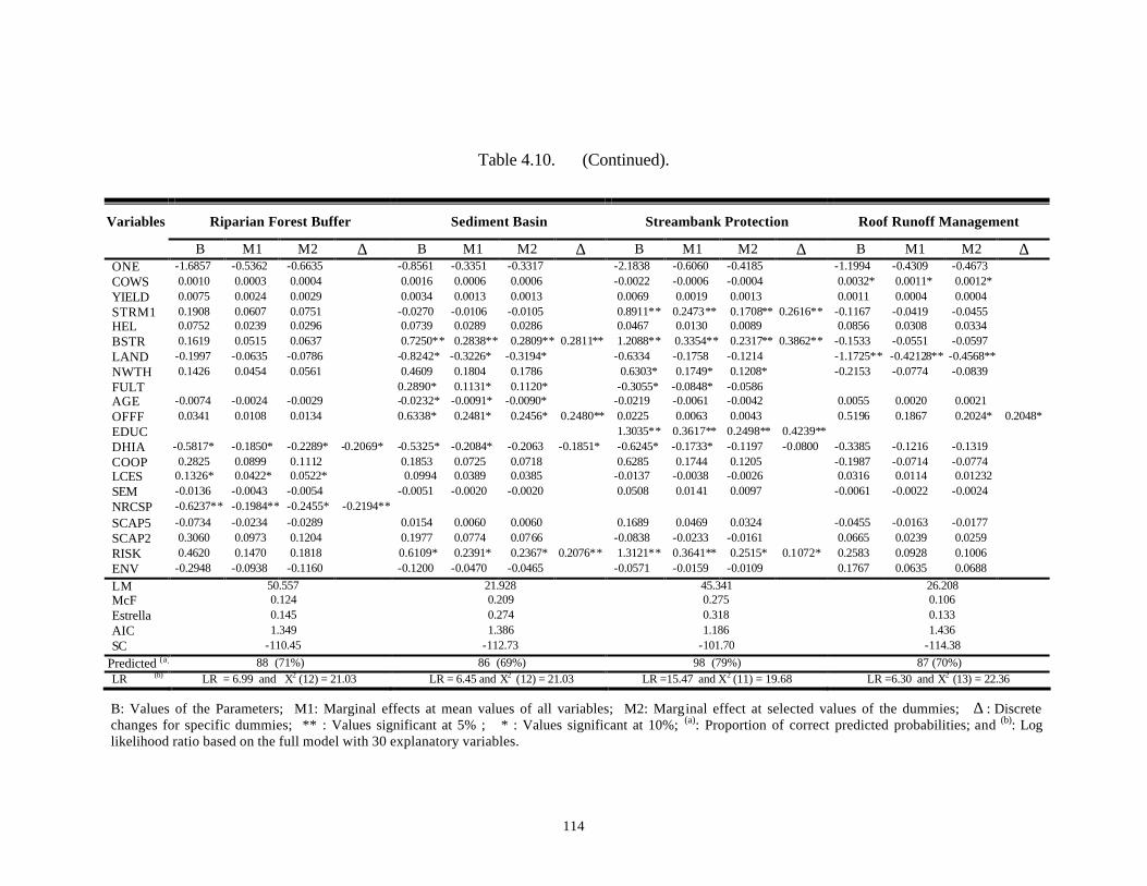
114
Table 4.10. (Continued).
Riparian Forest Buffer Sediment Basin Streambank Protection Roof Runoff Management Variables
B M1 M2 ∆ B M1 M2 ∆ B M1 M2 ∆ B M1 M2 ∆ ONE -1.6857 -0.5362 -0.6635 -0.8561 -0.3351 -0.3317 -2.1838 -0.6060 -0.4185 -1.1994 -0.4309 -0.4673 COWS 0.0010 0.0003 0.0004 0.0016 0.0006 0.0006 -0.0022 -0.0006 -0.0004 0.0032* 0.0011* 0.0012* YIELD 0.0075 0.0024 0.0029 0.0034 0.0013 0.0013 0.0069 0.0019 0.0013 0.0011 0.0004 0.0004 STRM1 0.1908 0.0607 0.0751 -0.0270 -0.0106 -0.0105 0.8911** 0.2473** 0.1708** 0.2616** -0.1167 -0.0419 -0.0455 HEL 0.0752 0.0239 0.0296 0.0739 0.0289 0.0286 0.0467 0.0130 0.0089 0.0856 0.0308 0.0334 BSTR 0.1619 0.0515 0.0637 0.7250** 0.2838** 0.2809** 0.2811** 1.2088** 0.3354** 0.2317** 0.3862** -0.1533 -0.0551 -0.0597 LAND -0.1997 -0.0635 -0.0786 -0.8242* -0.3226* -0.3194* -0.6334 -0.1758 -0.1214 -1.1725** -0.42128** -0.4568** NWTH 0.1426 0.0454 0.0561 0.4609 0.1804 0.1786 0.6303* 0.1749* 0.1208* -0.2153 -0.0774 -0.0839 FULT 0.2890* 0.1131* 0.1120* -0.3055* -0.0848* -0.0586 AGE -0.0074 -0.0024 -0.0029 -0.0232* -0.0091* -0.0090* -0.0219 -0.0061 -0.0042 0.0055 0.0020 0.0021 OFFF 0.0341 0.0108 0.0134 0.6338* 0.2481* 0.2456* 0.2480** 0.0225 0.0063 0.0043 0.5196 0.1867 0.2024* 0.2048* EDUC 1.3035** 0.3617** 0.2498** 0.4239** DHIA -0.5817* -0.1850* -0.2289* -0.2069* -0.5325* -0.2084* -0.2063 -0.1851* -0.6245* -0.1733* -0.1197 -0.0800 -0.3385 -0.1216 -0.1319 COOP 0.2825 0.0899 0.1112 0.1853 0.0725 0.0718 0.6285 0.1744 0.1205 -0.1987 -0.0714 -0.0774 LCES 0.1326* 0.0422* 0.0522* 0.0994 0.0389 0.0385 -0.0137 -0.0038 -0.0026 0.0316 0.0114 0.01232 SEM -0.0136 -0.0043 -0.0054 -0.0051 -0.0020 -0.0020 0.0508 0.0141 0.0097 -0.0061 -0.0022 -0.0024 NRCSP -0.6237** -0.1984** -0.2455* -0.2194** SCAP5 -0.0734 -0.0234 -0.0289 0.0154 0.0060 0.0060 0.1689 0.0469 0.0324 -0.0455 -0.0163 -0.0177 SCAP2 0.3060 0.0973 0.1204 0.1977 0.0774 0.0766 -0.0838 -0.0233 -0.0161 0.0665 0.0239 0.0259 RISK 0.4620 0.1470 0.1818 0.6109* 0.2391* 0.2367* 0.2076** 1.3121** 0.3641** 0.2515* 0.1072* 0.2583 0.0928 0.1006 ENV -0.2948 -0.0938 -0.1160 -0.1200 -0.0470 -0.0465 -0.0571 -0.0159 -0.0109 0.1767 0.0635 0.0688
LM 50.557 21.928 45.341 26.208 McF 0.124 0.209 0.275 0.106 Estrella 0.145 0.274 0.318 0.133 AIC 1.349 1.386 1.186 1.436 SC -110.45 -112.73 -101.70 -114.38
Predicted (a) 88 (71%) 86 (69%) 98 (79%) 87 (70%) LR (b) LR = 6.99 and X2 (12) = 21.03 LR = 6.45 and X2 (12) = 21.03 LR =15.47 and X2 (11) = 19.68 LR =6.30 and X2 (13) = 22.36
B: Values of the Parameters; M1: Marginal effects at mean values of all variables; M2: Marginal effect at selected values of the dummies; ∆ : Discrete changes for specific dummies; ** : Values significant at 5% ; * : Values significant at 10%; (a): Proportion of correct predicted probabilities; and (b): Log likelihood ratio based on the full model with 30 explanatory variables.
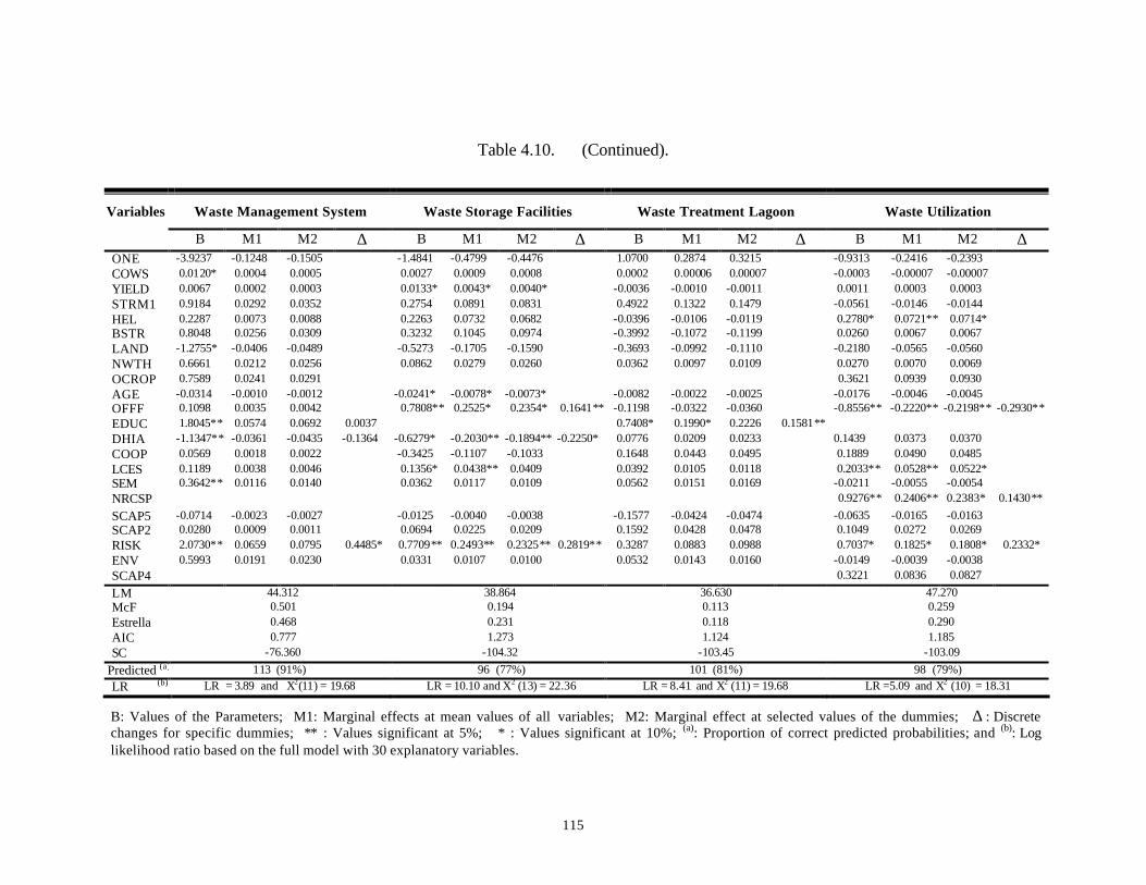
115
Table 4.10. (Continued).
Variables Waste Management System Waste Storage Facilities Waste Treatment Lagoon Waste Utilization
B M1 M2 ∆ B M1 M2 ∆ B M1 M2 ∆ B M1 M2 ∆ ONE -3.9237 -0.1248 -0.1505 -1.4841 -0.4799 -0.4476 1.0700 0.2874 0.3215 -0.9313 -0.2416 -0.2393 COWS 0.0120* 0.0004 0.0005 0.0027 0.0009 0.0008 0.0002 0.00006 0.00007 -0.0003 -0.00007 -0.00007 YIELD 0.0067 0.0002 0.0003 0.0133* 0.0043* 0.0040* -0.0036 -0.0010 -0.0011 0.0011 0.0003 0.0003 STRM1 0.9184 0.0292 0.0352 0.2754 0.0891 0.0831 0.4922 0.1322 0.1479 -0.0561 -0.0146 -0.0144 HEL 0.2287 0.0073 0.0088 0.2263 0.0732 0.0682 -0.0396 -0.0106 -0.0119 0.2780* 0.0721** 0.0714* BSTR 0.8048 0.0256 0.0309 0.3232 0.1045 0.0974 -0.3992 -0.1072 -0.1199 0.0260 0.0067 0.0067 LAND -1.2755* -0.0406 -0.0489 -0.5273 -0.1705 -0.1590 -0.3693 -0.0992 -0.1110 -0.2180 -0.0565 -0.0560 NWTH 0.6661 0.0212 0.0256 0.0862 0.0279 0.0260 0.0362 0.0097 0.0109 0.0270 0.0070 0.0069 OCROP 0.7589 0.0241 0.0291 0.3621 0.0939 0.0930 AGE -0.0314 -0.0010 -0.0012 -0.0241* -0.0078* -0.0073* -0.0082 -0.0022 -0.0025 -0.0176 -0.0046 -0.0045 OFFF 0.1098 0.0035 0.0042 0.7808** 0.2525* 0.2354* 0.1641** -0.1198 -0.0322 -0.0360 -0.8556** -0.2220** -0.2198** -0.2930** EDUC 1.8045** 0.0574 0.0692 0.0037 0.7408* 0.1990* 0.2226 0.1581** DHIA -1.1347** -0.0361 -0.0435 -0.1364 -0.6279* -0.2030** -0.1894** -0.2250* 0.0776 0.0209 0.0233 0.1439 0.0373 0.0370 COOP 0.0569 0.0018 0.0022 -0.3425 -0.1107 -0.1033 0.1648 0.0443 0.0495 0.1889 0.0490 0.0485 LCES 0.1189 0.0038 0.0046 0.1356* 0.0438** 0.0409 0.0392 0.0105 0.0118 0.2033** 0.0528** 0.0522* SEM 0.3642** 0.0116 0.0140 0.0362 0.0117 0.0109 0.0562 0.0151 0.0169 -0.0211 -0.0055 -0.0054 NRCSP 0.9276** 0.2406** 0.2383* 0.1430**
SCAP5 -0.0714 -0.0023 -0.0027 -0.0125 -0.0040 -0.0038 -0.1577 -0.0424 -0.0474 -0.0635 -0.0165 -0.0163 SCAP2 0.0280 0.0009 0.0011 0.0694 0.0225 0.0209 0.1592 0.0428 0.0478 0.1049 0.0272 0.0269 RISK 2.0730** 0.0659 0.0795 0.4485* 0.7709** 0.2493** 0.2325** 0.2819** 0.3287 0.0883 0.0988 0.7037* 0.1825* 0.1808* 0.2332* ENV 0.5993 0.0191 0.0230 0.0331 0.0107 0.0100 0.0532 0.0143 0.0160 -0.0149 -0.0039 -0.0038 SCAP4 0.3221 0.0836 0.0827
LM 44.312 38.864 36.630 47.270 McF 0.501 0.194 0.113 0.259 Estrella 0.468 0.231 0.118 0.290 AIC 0.777 1.273 1.124 1.185 SC -76.360 -104.32 -103.45 -103.09
Predicted (a) 113 (91%) 96 (77%) 101 (81%) 98 (79%) LR (b) LR = 3.89 and X2(11) = 19.68 LR = 10.10 and X2 (13) = 22.36 LR = 8.41 and X2 (11) = 19.68 LR =5.09 and X2 (10) = 18.31
B: Values of the Parameters; M1: Marginal effects at mean values of all variables; M2: Marginal effect at selected values of the dummies; ∆ : Discrete changes for specific dummies; ** : Values significant at 5%; * : Values significant at 10%; (a): Proportion of correct predicted probabilities; and (b): Log likelihood ratio based on the full model with 30 explanatory variables.
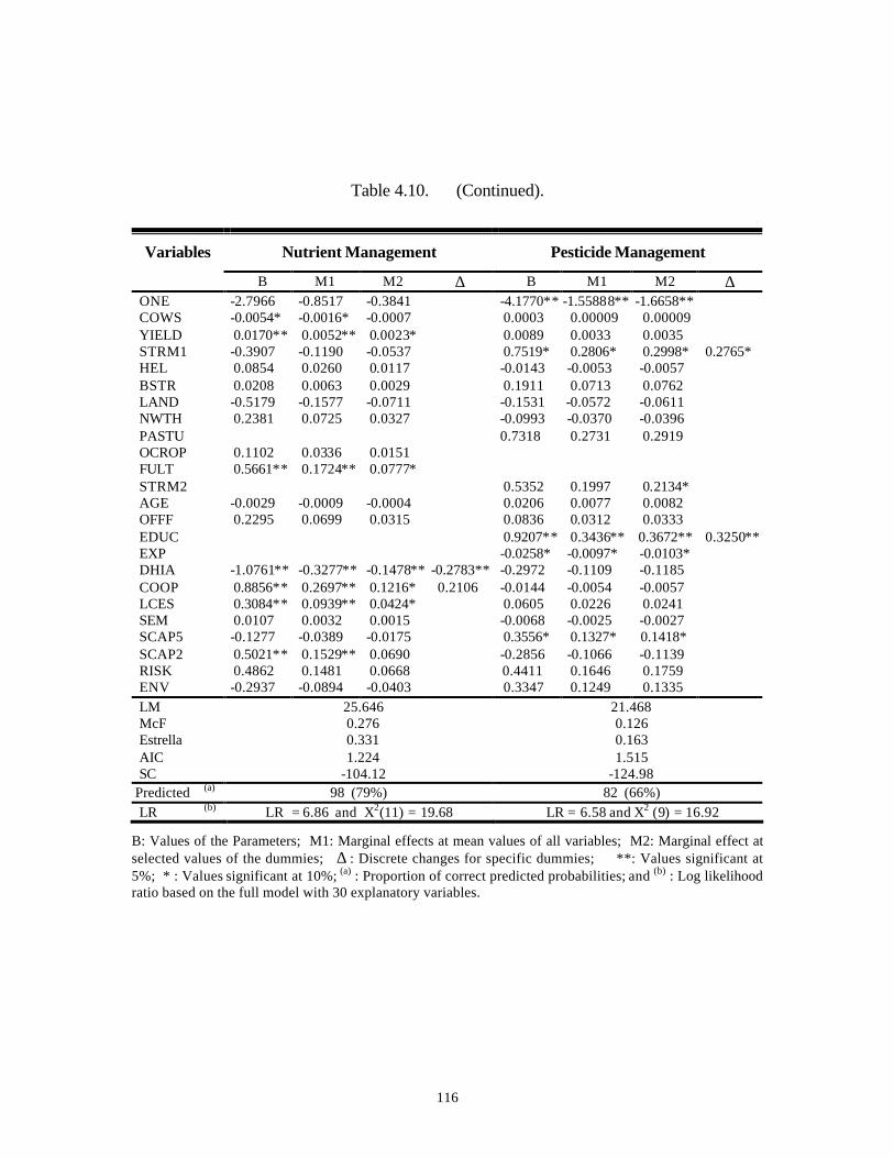
116
Table 4.10. (Continued).
Nutrient Management Pesticide Management Variables
B M1 M2 ∆ B M1 M2 ∆ ONE -2.7966 -0.8517 -0.3841 -4.1770** -1.55888** -1.6658** COWS -0.0054* -0.0016* -0.0007 0.0003 0.00009 0.00009 YIELD 0.0170** 0.0052** 0.0023* 0.0089 0.0033 0.0035 STRM1 -0.3907 -0.1190 -0.0537 0.7519* 0.2806* 0.2998* 0.2765* HEL 0.0854 0.0260 0.0117 -0.0143 -0.0053 -0.0057 BSTR 0.0208 0.0063 0.0029 0.1911 0.0713 0.0762 LAND -0.5179 -0.1577 -0.0711 -0.1531 -0.0572 -0.0611 NWTH 0.2381 0.0725 0.0327 -0.0993 -0.0370 -0.0396 PASTU 0.7318 0.2731 0.2919 OCROP 0.1102 0.0336 0.0151 FULT 0.5661** 0.1724** 0.0777* STRM2 0.5352 0.1997 0.2134* AGE -0.0029 -0.0009 -0.0004 0.0206 0.0077 0.0082 OFFF 0.2295 0.0699 0.0315 0.0836 0.0312 0.0333 EDUC 0.9207** 0.3436** 0.3672** 0.3250** EXP -0.0258* -0.0097* -0.0103* DHIA -1.0761** -0.3277** -0.1478** -0.2783** -0.2972 -0.1109 -0.1185 COOP 0.8856** 0.2697** 0.1216* 0.2106 -0.0144 -0.0054 -0.0057 LCES 0.3084** 0.0939** 0.0424* 0.0605 0.0226 0.0241 SEM 0.0107 0.0032 0.0015 -0.0068 -0.0025 -0.0027 SCAP5 -0.1277 -0.0389 -0.0175 0.3556* 0.1327* 0.1418* SCAP2 0.5021** 0.1529** 0.0690 -0.2856 -0.1066 -0.1139 RISK 0.4862 0.1481 0.0668 0.4411 0.1646 0.1759 ENV -0.2937 -0.0894 -0.0403 0.3347 0.1249 0.1335 LM 25.646 21.468 McF 0.276 0.126 Estrella 0.331 0.163 AIC 1.224 1.515 SC -104.12 -124.98
Predicted (a) 98 (79%) 82 (66%) LR (b) LR = 6.86 and X2(11) = 19.68 LR = 6.58 and X2 (9) = 16.92
B: Values of the Parameters; M1: Marginal effects at mean values of all variables; M2: Marginal effect at selected values of the dummies; ∆ : Discrete changes for specific dummies; **: Values significant at 5%; * : Values significant at 10%; (a) : Proportion of correct predicted probabilities; and (b) : Log likelihood ratio based on the full model with 30 explanatory variables.
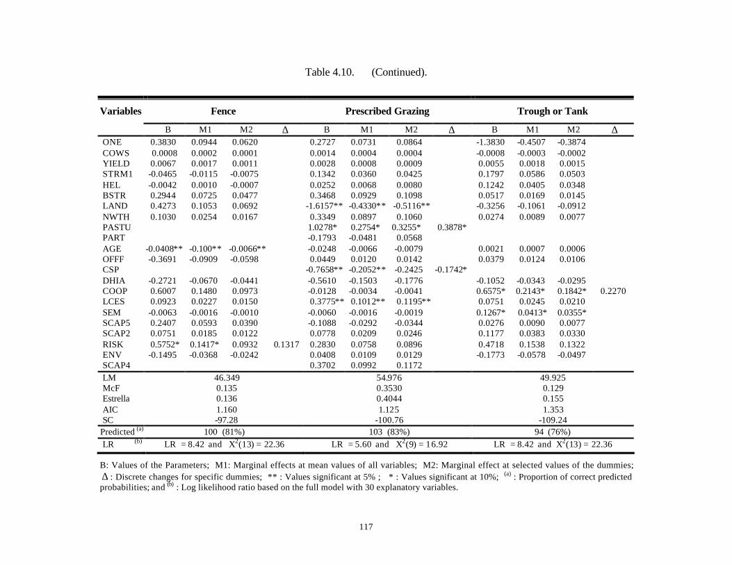
117
Table 4.10. (Continued).
Fence Prescribed Grazing Trough or Tank Variables
B M1 M2 ∆ B M1 M2 ∆ B M1 M2 ∆ ONE 0.3830 0.0944 0.0620 0.2727 0.0731 0.0864 -1.3830 -0.4507 -0.3874 COWS 0.0008 0.0002 0.0001 0.0014 0.0004 0.0004 -0.0008 -0.0003 -0.0002 YIELD 0.0067 0.0017 0.0011 0.0028 0.0008 0.0009 0.0055 0.0018 0.0015 STRM1 -0.0465 -0.0115 -0.0075 0.1342 0.0360 0.0425 0.1797 0.0586 0.0503 HEL -0.0042 0.0010 -0.0007 0.0252 0.0068 0.0080 0.1242 0.0405 0.0348 BSTR 0.2944 0.0725 0.0477 0.3468 0.0929 0.1098 0.0517 0.0169 0.0145 LAND 0.4273 0.1053 0.0692 -1.6157** -0.4330** -0.5116** -0.3256 -0.1061 -0.0912 NWTH 0.1030 0.0254 0.0167 0.3349 0.0897 0.1060 0.0274 0.0089 0.0077 PASTU 1.0278* 0.2754* 0.3255* 0.3878* PART -0.1793 -0.0481 0.0568 AGE -0.0408** -0.100** -0.0066** -0.0248 -0.0066 -0.0079 0.0021 0.0007 0.0006 OFFF -0.3691 -0.0909 -0.0598 0.0449 0.0120 0.0142 0.0379 0.0124 0.0106 CSP -0.7658** -0.2052** -0.2425 -0.1742* DHIA -0.2721 -0.0670 -0.0441 -0.5610 -0.1503 -0.1776 -0.1052 -0.0343 -0.0295 COOP 0.6007 0.1480 0.0973 -0.0128 -0.0034 -0.0041 0.6575* 0.2143* 0.1842* 0.2270 LCES 0.0923 0.0227 0.0150 0.3775** 0.1012** 0.1195** 0.0751 0.0245 0.0210 SEM -0.0063 -0.0016 -0.0010 -0.0060 -0.0016 -0.0019 0.1267* 0.0413* 0.0355* SCAP5 0.2407 0.0593 0.0390 -0.1088 -0.0292 -0.0344 0.0276 0.0090 0.0077 SCAP2 0.0751 0.0185 0.0122 0.0778 0.0209 0.0246 0.1177 0.0383 0.0330 RISK 0.5752* 0.1417* 0.0932 0.1317 0.2830 0.0758 0.0896 0.4718 0.1538 0.1322 ENV -0.1495 -0.0368 -0.0242 0.0408 0.0109 0.0129 -0.1773 -0.0578 -0.0497 SCAP4 0.3702 0.0992 0.1172 LM 46.349 54.976 49.925 McF 0.135 0.3530 0.129 Estrella 0.136 0.4044 0.155 AIC 1.160 1.125 1.353 SC -97.28 -100.76 -109.24
Predicted (a) 100 (81%) 103 (83%) 94 (76%) LR (b) LR = 8.42 and X2(13) = 22.36 LR = 5.60 and X2(9) = 16.92 LR = 8.42 and X2(13) = 22.36
B: Values of the Parameters; M1: Marginal effects at mean values of all variables; M2: Marginal effect at selected values of the dummies; ∆ : Discrete changes for specific dummies; ** : Values significant at 5% ; * : Values significant at 10%; (a) : Proportion of correct predicted probabilities; and (b) : Log likelihood ratio based on the full model with 30 explanatory variables.
118
The negative sign for variable LAND could be due to the larger percentage of owned
land among smaller-sized farms that did not adopt conservation tillage practices. Holding other
variables constant, a one percent increase in land owned would likely reduce the probability of
adopting conservation tillage practices by 38 percent, and membership in a milk cooperative
would decrease the probability by 23 percent. Having an off- farm job would, on the other hand,
increase the probability of adopting by 18 percent. This is not surprising since conservation
tillage generally requires less labor than conventional tillage, and the off- farm employee is likely
to be labor-constrained. The model also shows that producers who rated relationships with
regulatory agencies as more important were less likely to adopt, as suggested by the 15 percent
decrease in the probability of adopting conservation tillage, associated with variable SCAP5.
Such result was not as initially expected.
The model for the cover green manure crop practice included the 17 variables from the
PCA. YIELD was the only significant variable, though the effect was very small. A 100 pound
increase in cow productivity would increase the probability of adopting the practice by 0.5
percent, holding other variables constant. COWS, YIELD and membership in DHIA
significantly influenced the adoption of the critical area planting practice. The negative sign of
the DHIA variable was not as initially expected. The effect may be because of the purposes of
DHIA in enhancing dairy operation productivity and ensuring higher profit through highly
monitored business management. Adoption of conservation practices, on the other hand, aims at
an overall improvement of the environment which would ensure long term financial outcomes.
Thus, adoption of this BMP (and others as will later be seen) may not be consistent with the
goals of profit maximizing producers. Membership in DHIA would likely reduce the probability
of adopting critical area planting by 26 percent, holding the other variables constant.
119
The probit model for the field borders practice included 19 explanatory variables, five of
which significantly influenced the probability of adopting the practice. The positive effects of
COWS, YIELD, TOVR, and LCES variables were as expected. With respect to the negative
effect of SCAP4 variable, a good relationship with non-farmer neighbors would reduce the
probability of establishing perennial vegetation at the edge of the field by 23 percent, holding the
other variables constant. This may be due to a perception that such vegetation is unsightly and,
thus, un-neighborly. Having any family member planning to take over the farm operation upon
the producer’s retirement would likely increase the probability to establish field borders by 23
percent, holding the other variables constant.
Variables COWS, YIELD and DHIA significantly affected the adoption of filter strips.
The magnitude of the positive effects of COWS and YIELD were again relatively small, about
0.001 and 0.007, respectively. Membership in DHIA would decrease the probability of
establishing vegetative areas to trap sediment, organic material, nutrients and chemicals from
runoff by 20 percent, holding other variables constant.
The adoption of grassed waterways was significantly influenced by five variables:
YIELD, HEL, DHIA, LCES, and RISK. The signs of the effects were as expected. A twenty
percent increase in farmland classified as “highly erodible” would result in an increased
probability to construct grassed waterway channels of 13 percent, holding other variables
constant. One additional meeting with LCES and producer’s risk aversion would likely increase
the adoption by 4 and 25 percent, respectively, holding the other variables constant. The risk
averse producer might adopt grassed waterways to reduce the potential negative impact of a
heavy rain event on the long-run productivity and economic viability of the land.
120
Producers’ decisions to stabilize frequently and intensively used areas were significantly
affected by the level of their debt/asset ratio. A twenty percent increase in the ratio would likely
decrease the probability of protecting heavy use areas by 9 percent, holding the other variables
constant.
Memberships in milk cooperatives as well as in DHIA had significant impacts on the
adoption of regulating in a water drainage system. The effects, although similar in magnitude,
were in the opposite direction. DHIA would likely reduce the probability to adopt the practice
by 21 percent, whereas COOP would likely enhance the adoption by 24 percent, holding the
other variables constant. Many COOP newsletters inform producers about dairy management
issues, allowing them to make better informed management decisions.
Three variables significantly affected the adoption of riparian forest buffers. Membership
in DHIA, and a plan established with NRCS would likely decrease the probability to establish
buffer zones adjacent to and uphill from water bodies by 21 and 22 percent, respectively. An
additional meeting with LCES, on the other hand would enhance the adoption by 5 percent.
Seven variables significantly influenced the construction of sediment basins. Business
structured as a corporation, number of fulltime workers, the holding of an off- farm job, and
farmer’s risk aversion were associated with increased adoption of the practice. Increases in the
probability to construct a sediment basin associated with these three dummy variables were 28,
25 and 21 percent, respectively. Having one additional fulltime worker would increase the
probability of constructing sediment basins by 11 percent. On the other hand, a larger
percentage of land owned, age and membership in DHIA reduced the adoption. A one unit
increase in the percentage of land owned, one year of age older, and membership in DHIA would
reduce the probability to construct sediment basins by 32, 0.9 and 19 percent, respectively.
121
The positive effects of having a stream and/or river running through the farmland,
business structured as a corporation, higher net worth, education and risk aversion on the
establishment of vegetation or structures to protect banks of streams from erosion were as
expected. The increased effects on the probability of protecting streambanks and shorelines,
associated with these four variables were 26, 38, 42, and 11 percent, respectively. The hiring of
one additional fulltime worker and membership in DHIA would reduce the probability of
adoption by 6 and 8 percent, respectively.
4.2.3.2. Facility Wastewater and Runoff Management Practices
Having a larger sized farm and the holding of an off- farm job enhanced the adoption of
roof runoff management. These two variables were associated with marginal increases of 0.1
and 20 percent, respectively, in the probability to adopt the practice. A one percent increase in
the land owned would reduce the probability to manage roof runoff by 46 percent.
The probit model for the waste management system included 20 variables, six of which
had significant β coefficients. However, their effects on the probability to adopt the practice
were not significant except for the RISK variable. Producer’s aversion to risk would increase the
probability of adopting a system to manage waste by 45 percent.
Four variables significantly and positively influenced the increased construction of a
waste storage impoundment. Cow productivity, the holding of an off- farm job, frequency of
meetings with LCES and farmers’ risk aversion increased the probability of adopting a waste
storage facility. These variables were associated with an increased probability of constructing a
waste impoundment of 0.4, 16, 4, and 28 percent, respectively, holding the other variables
constant. On the other hand, Age and DHIA membership negatively affected the adoption. One
year of age older and membership in DHIA would decrease the probability to adopt by 0.7 and
122
23 percent, respectively. The probit model for waste treatment lagoon included 20 variables.
Producer’s educational attainment was the only variable that significantly influenced producer’s
adoption of the practice. Having a college degree would increase the probability of adopting by
16 percent.
Higher percentage of farmland classified as “highly erodible”, frequency of meetings
with LCES, the establishment of a dairy farm plan with NRCS, and farmer’ s risk aversion were
associated with proper utilization of wastes. The increased effects on the probability of adoption
were 7, 14 and 23 percent, respectively. The holding of an off- farm job would reduce the
probability of adopting the practice by 29 percent. The spreading of manure is very labor
intensive, perhaps preventing producers with off farm employment from doing it.
4.2.3.3. Nutrient and Pesticide Management
The probit model for nutrient management included 19 variables and six variables were
found to significantly influence farmers’ decisions to adopt the practice. Milk yield, the number
of full time employees, membership in a milk cooperative, frequency of meetings with LCES,
and a good relationship with lending institutions were associated with greater implementation of
nutrient management. A higher number of cows and membership in DHIA would likely
decrease the adoption of nutrient management. The effect of cows is surprising, given the
increased scrutiny of regulatory agencies, especially with respect to larger operations.
The existence of a stream and/or river running through the farm, higher educational
attainment and good a relationship with regulatory agencies were found to be positively
associated with enhanced adoption of pesticide management. Dairy producers who have been in
business longer have likely become more accustomed to existing practices and less likely to
change, thus explaining the negative coefficient on experience.
123
4.2.3.4. Grazing Management
The probit model for fencing practice included the 17 variables retained from the PCA.
Age and risk aversion were the two variables which significantly influenced the dairy producers’
adoption of the practice. One year of age older would decrease the probability of adopting by 7
percent, whereas, risk aversion would increase the adoption by 13 percent.
Producers operating a pasture-based dairy farm and meeting frequently with LCES
personnel would be more likely to adopt prescribed grazing. The increased effects of the
PASTU and LCES variables on the probability that a dairy producer would establish a prescribed
grazing plan would be 39 and 12 percent, respectively. A one percent increase in land owned
and participation in a cost-sharing program would reduce the probability of adopting by 51 and
17 percent, respectively. These negative effects of LAND and CSP are not as initially expected.
Membership in a milk cooperative and frequent attendance of seminars and/or meetings that
dealt with dairy industry issues were associated with greater implementation of livestock
watering facilities such as a trough or tank. These variables were associated with 22 and 4
percent increases in the probability of adopting, respectively.
4.2.4. Bivariate Probit Analysis
The simultaneous adoption of two BMPs was examined in this section. The system of
two equations in the bivariate probit model was based on the selected models from the univariate
probit analysis. The group of practices which aimed at erosion and sediment control was divided
into two subcategories according to whether they targeted primarily erosion reduction or
sediment control. In total, 38 bivariate models were estimated for the 21 BMPs, as shown in
Table 4.11. Twenty-one models were explored for the seven practices included in the subgroup
of practices targeting the reduction of erosion, and six models were analyzed for the group of
124
practices for sediment control. Waste storage facility, waste treatment lagoon, and waste
utilization were considered as nested in the waste management system. Therefore, the number of
bivariate estimations was reduced to 7 for the group of practices dealing with facility wastewater
and runoff management. The 4 remaining estimations concerned nutrient and pesticide
management and the grazing management practices.
Thirty-two of the rho coefficients were found significant at the 5 or 10 percent levels of
significance. Results also showed few strong correlations of 0.8 or more. Comparison of the
initial frequency of dependent variable outcomes (0,0), (0,1), (1,0) and (1,1) with the fitted
values provided information about model predictability. The bivariate probit models for the
group of practices targeting erosion and sediment control tended to heavily predict the adoption
of neither practices under consideration. This may be due to the low adoption rate of most of the
erosion and sediment control practices. Marginal effects of the explanatory variables were
estimated conditional on the adoption of one practice. All the Lagrange Multiplier statistical
values were associated with very large p-values, allowing one to conclude no problem with
heteroskedasticity. The goodness of fit of the model was assessed using the pseudo-R2 measure
used by Lim-Applegate et al. (2002).
Selected results for the bivariate probit models are summarized in Table 4.12. The
bivariate probit model for field borders and grassed waterways included in total 38 independent
variables. The holding of an off- farm job, plans for a family member to take over the dairy
operation upon the farmer’s retirement, frequency of meetings with LCES personnel, and good
relationships with non-farmer neighbors were associated with an increased joint adoption of field
borders and grassed waterways. The negative effect of variable SCAP4 on the conditional
probability of establishing any field borders given that grassed waterways practice was adopted,
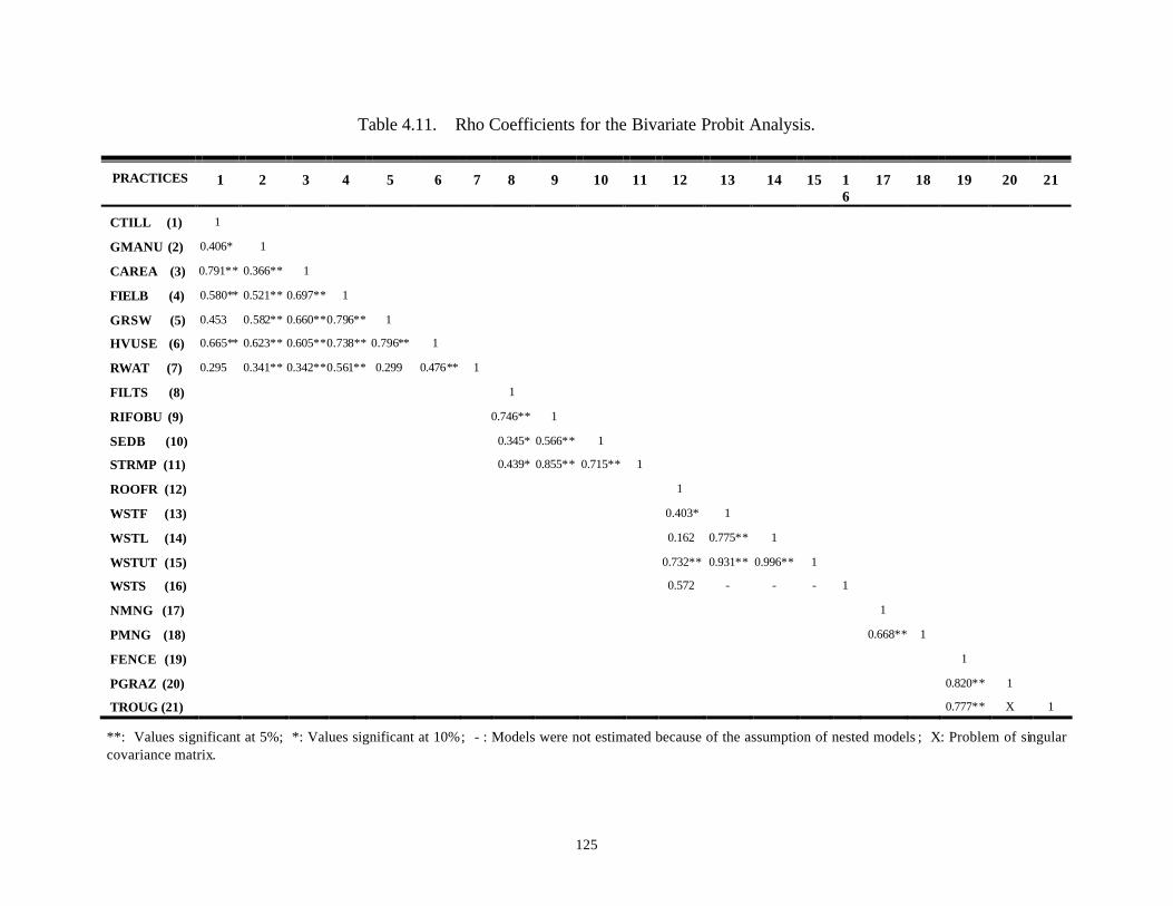
125
Table 4.11. Rho Coefficients for the Bivariate Probit Analysis.
PRACTICES 1 2 3 4 5 6 7 8 9 10 11 12 13 14 15 16
17 18 19 20 21
CTILL (1) 1
GMANU (2) 0.406* 1
CAREA (3) 0.791** 0.366** 1
FIELB (4) 0.580** 0.521** 0.697** 1
GRSW (5) 0.453 0.582** 0.660**0.796** 1
HVUSE (6) 0.665** 0.623** 0.605**0.738** 0.796** 1
RWAT (7) 0.295 0.341** 0.342**0.561** 0.299 0.476** 1
FILTS (8) 1
RIFOBU (9) 0.746** 1
SEDB (10) 0.345* 0.566** 1
STRMP (11) 0.439* 0.855** 0.715** 1
ROOFR (12) 1
WSTF (13) 0.403* 1
WSTL (14) 0.162 0.775** 1
WSTUT (15) 0.732** 0.931** 0.996** 1
WSTS (16) 0.572 - - - 1
NMNG (17) 1
PMNG (18) 0.668** 1
FENCE (19) 1
PGRAZ (20) 0.820** 1
TROUG (21) 0.777** X 1
**: Values significant at 5%; *: Values significant at 10%; - : Models were not estimated because of the assumption of nested models ; X: Problem of singular covariance matrix.
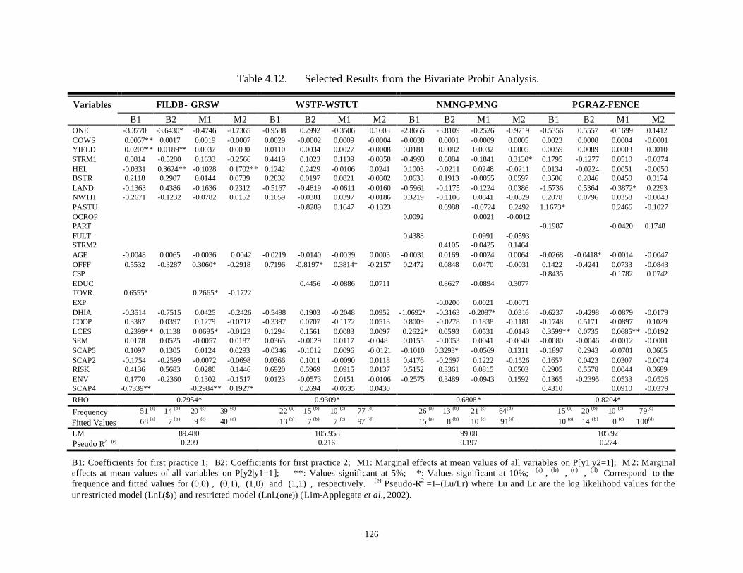
126
Table 4.12. Selected Results from the Bivariate Probit Analysis.
Variables FILDB- GRSW WSTF-WSTUT NMNG-PMNG PGRAZ-FENCE
B1 B2 M1 M2 B1 B2 M1 M2 B1 B2 M1 M2 B1 B2 M1 M2 ONE -3.3770 -3.6430* -0.4746 -0.7365 -0.9588 0.2992 -0.3506 0.1608 -2.8665 -3.8109 -0.2526 -0.9719 -0.5356 0.5557 -0.1699 0.1412 COWS 0.0057** 0.0017 0.0019 -0.0007 0.0029 -0.0002 0.0009 -0.0004 -0.0038 0.0001 -0.0009 0.0005 0.0023 0.0008 0.0004 -0.0001 YIELD 0.0207** 0.0189** 0.0037 0.0030 0.0110 0.0034 0.0027 -0.0008 0.0181 0.0082 0.0032 0.0005 0.0059 0.0089 0.0003 0.0010 STRM1 0.0814 -0.5280 0.1633 -0.2566 0.4419 0.1023 0.1139 -0.0358 -0.4993 0.6884 -0.1841 0.3130* 0.1795 -0.1277 0.0510 -0.0374 HEL -0.0331 0.3624** -0.1028 0.1702** 0.1242 0.2429 -0.0106 0.0241 0.1003 -0.0211 0.0248 -0.0211 0.0134 -0.0224 0.0051 -0.0050 BSTR 0.2118 0.2907 0.0144 0.0739 0.2832 0.0197 0.0821 -0.0302 0.0633 0.1913 -0.0055 0.0597 0.3506 0.2846 0.0450 0.0174 LAND -0.1363 0.4386 -0.1636 0.2312 -0.5167 -0.4819 -0.0611 -0.0160 -0.5961 -0.1175 -0.1224 0.0386 -1.5736 0.5364 -0.3872* 0.2293 NWTH -0.2671 -0.1232 -0.0782 0.0152 0.1059 -0.0381 0.0397 -0.0186 0.3219 -0.1106 0.0841 -0.0829 0.2078 0.0796 0.0358 -0.0048 PASTU -0.8289 0.1647 -0.1323 0.6988 -0.0724 0.2492 1.1673* 0.2466 -0.1027 OCROP 0.0092 0.0021 -0.0012 PART -0.1987 -0.0420 0.1748 FULT 0.4388 0.0991 -0.0593 STRM2 0.4105 -0.0425 0.1464 AGE -0.0048 0.0065 -0.0036 0.0042 -0.0219 -0.0140 -0.0039 0.0003 -0.0031 0.0169 -0.0024 0.0064 -0.0268 -0.0418* -0.0014 -0.0047 OFFF 0.5532 -0.3287 0.3060* -0.2918 0.7196 -0.8197* 0.3814* -0.2157 0.2472 0.0848 0.0470 -0.0031 0.1422 -0.4241 0.0733 -0.0843 CSP -0.8435 -0.1782 0.0742 EDUC 0.4456 -0.0886 0.0711 0.8627 -0.0894 0.3077 TOVR 0.6555* 0.2665* -0.1722 EXP -0.0200 0.0021 -0.0071 DHIA -0.3514 -0.7515 0.0425 -0.2426 -0.5498 0.1903 -0.2048 0.0952 -1.0692* -0.3163 -0.2087* 0.0316 -0.6237 -0.4298 -0.0879 -0.0179 COOP 0.3387 0.0397 0.1279 -0.0712 -0.3397 0.0707 -0.1172 0.0513 0.8009 -0.0278 0.1838 -0.1181 -0.1748 0.5171 -0.0897 0.1029 LCES 0.2399** 0.1138 0.0695* -0.0123 0.1294 0.1561 0.0083 0.0097 0.2622* 0.0593 0.0531 -0.0143 0.3599** 0.0735 0.0685** -0.0192 SEM 0.0178 0.0525 -0.0057 0.0187 0.0365 -0.0029 0.0117 -0.048 0.0155 -0.0053 0.0041 -0.0040 -0.0080 -0.0046 -0.0012 -0.0001 SCAP5 0.1097 0.1305 0.0124 0.0293 -0.0346 -0.1012 0.0096 -0.0121 -0.1010 0.3293* -0.0569 0.1311 -0.1897 0.2943 -0.0701 0.0665 SCAP2 -0.1754 -0.2599 -0.0072 -0.0698 0.0366 0.1011 -0.0090 0.0118 0.4176 -0.2697 0.1222 -0.1526 0.1657 0.0423 0.0307 -0.0074 RISK 0.4136 0.5683 0.0280 0.1446 0.6920 0.5969 0.0915 0.0137 0.5152 0.3361 0.0815 0.0503 0.2905 0.5578 0.0044 0.0689 ENV 0.1770 -0.2360 0.1302 -0.1517 0.0123 -0.0573 0.0151 -0.0106 -0.2575 0.3489 -0.0943 0.1592 0.1365 -0.2395 0.0533 -0.0526 SCAP4 -0.7339** -0.2984** 0.1927* 0.2694 -0.0535 0.0430 0.4310 0.0910 -0.0379 RHO 0.7954* 0.9309* 0.6808* 0.8204*
Frequency 51 (a) 14 (b) 20 (c) 39 (d) 22 (a) 15 (b) 10 (c) 77 (d) 26 (a) 13 (b) 21 (c) 64(d) 15 (a) 20 (b) 10 (c) 79(d)
Fitted Values 68 (a) 7 (b) 9 (c) 40 (d) 13 (a) 7 (b) 7 (c) 97 (d) 15 (a) 8 (b) 10 (c) 91(d) 10 (a) 14 (b) 0 (c) 100(d)
LM 89.480 105.958 99.08 105.92 Pseudo R2 (e) 0.209 0.216 0.197 0.274
B1: Coefficients for first practice 1; B2: Coefficients for first practice 2; M1: Marginal effects at mean values of all variables on P[y1|y2=1]; M2: Marginal effects at mean values of all variables on P[y2|y1=1]; **: Values significant at 5%; *: Values significant at 10%; (a) , (b) , (c) , (d) Correspond to the frequence and fitted values for (0,0) , (0,1), (1,0) and (1,1) , respectively. (e) Pseudo-R2 =1–(Lu/Lr) where Lu and Lr are the log likelihood values for the unrestricted model (LnL($)) and restricted model (LnL(one)) (Lim-Applegate et al., 2002).
127
is similar to tha t encountered in the univariate probit model for field borders. A good
relationship with non-farmer neighbors would reduce the probability of establishing perennial
vegetation at the edge of the field by 29 percent if grassed waterways had been established. On
the other hand, percentage of farm land classified as “highly erodible” and good relationships
with neighbors were associated with increased construction of grassed waterways by dairy
farmers who had established field borders.
The model for waste storage facility and waste utilization included 39 variables. The
distribution of the fitted values associated the model with higher predictions on the adoption of
both practices (78 percent) and relatively less on the adoption of neither one (10 percent)
compared to the initial frequency of the dependent variable outcomes. The holding of an off-
farm job was the only variable which significantly affected the adoption of both practices. It
increased the probability of constructing temporary storage impoundments given that the dairy
producers had adopted proper utilization of wastes by 38 percent.
The model for nutrient and pesticide management included 42 variables in total. The rho
coefficient of 0.68 was significant at the 5 percent level of significance. The model predicted an
increased adoption of both practices simultaneously. Three variables were found to significantly
affect the joint adoption. The directions of the effects, reflected in the signs of the estimated
coefficients, were consistent with the findings in the probit analysis of each BMP. Membership
in DHIA likely reduced the implementation of nutrient management if the dairy farmer had
adopted pesticide management. Having a stream and/or river running through the farm likely
increased the adoption of pesticide management by dairy farmers who had a nutrient
management plan.
128
The bivariate probit model for prescribed gazing and fencing practices had a rho
coefficient of 0.82, significant at the 5 percent level. This model also predicted a higher
percentage (81 percent) of adopting both practices simultaneously compared to the initial
frequency of the dependent variables outcomes. The signs of the coefficients associated with
variables PASTU, AGE and LCES were similar to those in the univariate probit models. One
additional meeting with LCES personnel would increase the establishment of a prescribed
grazing plan by dairy farmers who had fenced their land by 7 percent. One percent additional
land owned to total land in the farm operation would decrease the adoption by 39 percent.
4.2.5. Multivariate Probit Analysis
The simultaneous adoption of larger sets of BMPs in each subgroup of practices were
examined in this section. Variables to be included in the system of 3 to 6 equations in the
multivariate probit analysis were determined using 4 different scenarios. In the first scenario,
variables were based on the selected models from the univariate probit analysis. In scenario two,
each equation incorporated the 12 variables obtained from the PCA ( 1)λ = . These models were
extended in scenario three by including other variables significant at least at the 10 percent level,
from the probit analysis of each BMP. Models in scenario four included variables from the
probit analysis, which were significant at least at the 50 percent level of significance. Discrete
changes in the probability of adopting all practices under consideration were estimated as
alternative to marginal effects of variables associated with coefficients with significance at least
at the 10 percent level.
4.2.5.1. Erosion and Sediment Control Practices
Two sets of models were considered for the group of practices targeting erosion reduction
labeled category I in Table 4.13. Conservation tillage was left out because of its relatively high
129
rate of adoption compared to the remaining practices in the group. Indeed, conservation tillage
was adopted at the rate of 77 percent while the adoption rates of the remaining erosion and
sediment practices were from 28 to 48 percent. Such a difference would affect the estimation.
The first set of models included six equations associated with the following practices:
cover and green manure crop (GMANU), critical area planting (CAREA), field borders
(FILDB), grassed waterways (GRSW), heavy use area protection (HVUSE) and regulating water
in drainage systems (RWAT). Results from the four scenarios showed the following: estimation
of scenarios one and four encountered singular covariance matrices, and models in scenarios two
and three were successfully estimated but did not yield any significant variables.
According to Donny Latiolais, cover and green manure crop have not been used much in
the southeastern region of Louisiana. Since most of the respondents were from that region,
GMANU was left out of the second set of models for the group of practices targeting erosion
reduction. Estimations in scenarios two and three were successful but did not yield any
significant variables. Estimation of the model in scenario four yielded the largest log likelihood
value. The β coefficient associated with YIELD was significant at the 10 percent level, as
shown in Table 4.14. The value of the discrete change suggested that an increase of 100 lbs of
milk in the productivity per cow would increase the probability to adopt all five practices
simultaneously by 0.2 percent.
Two sets of models were considered for the group of practices for sediment control
purposes labeled category II in Table 4.13. The first set of models included all four practices:
filter strips (FILTS), sediment basin (SEDB), riparian forest buffers (RIFOBU), and streambank
and shoreline protection (STRMP). Estimations of the models in scenario s one and four resulted
in singular covariance matrices. Models in scenarios two and three were successfully estimated.
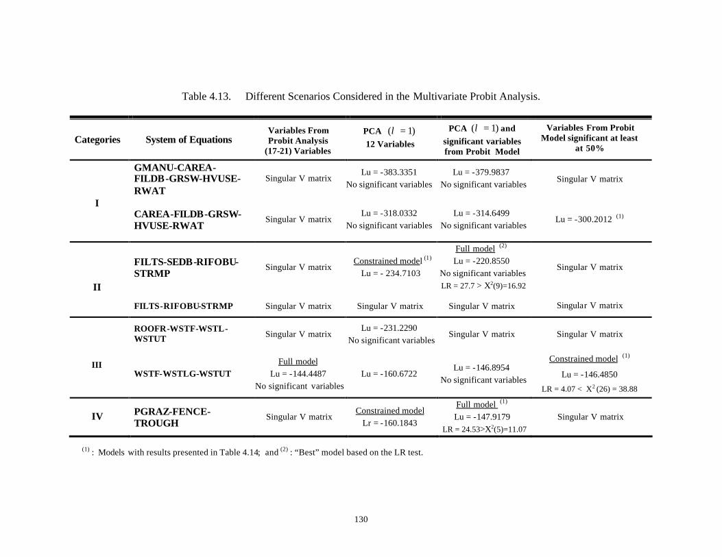
130
Table 4.13. Different Scenarios Considered in the Multivariate Probit Analysis.
Categories System of Equations Variables From Probit Analysis
(17-21) Variables
PCA ( 1)λ = 12 Variables
PCA ( 1)λ = and significant variables from Probit Model
Variables From Probit Model significant at least
at 50%
GMANU-CAREA-FILDB-GRSW-HVUSE-RWAT
Singular V matrix Lu = -383.3351
No significant variables Lu = -379.9837
No significant variables Singular V matrix
I CAREA-FILDB-GRSW-HVUSE-RWAT
Singular V matrix Lu = -318.0332
No significant variables Lu = -314.6499
No significant variables Lu = -300.2012 (1)
FILTS-SEDB-RIFOBU-STRMP
Singular V matrix Constrained model (1)
Lu = - 234.7103
Full model (2)
Lu = -220.8550 No significant variables LR = 27.7 > X2(9)=16.92
Singular V matrix
II
FILTS-RIFOBU-STRMP Singular V matrix Singular V matrix Singular V matrix Singular V matrix
ROOFR-WSTF-WSTL-WSTUT Singular V matrix
Lu = -231.2290 No significant variables
Singular V matrix Singular V matrix
III WSTF-WSTLG-WSTUT
Full model Lu = -144.4487
No significant variables
Lu = -160.6722
Lu = -146.8954 No significant variables
Constrained model (1)
Lu = -146.4850
LR = 4.07 < X2 (26) = 38.88
IV PGRAZ-FENCE-TROUGH
Singular V matrix Constrained model
Lr = -160.1843
Full model (1)
Lu = -147.9179 LR = 24.53>X2(5)=11.07
Singular V matrix
(1) : Models with results presented in Table 4.14; and (2) : “Best” model based on the LR test.
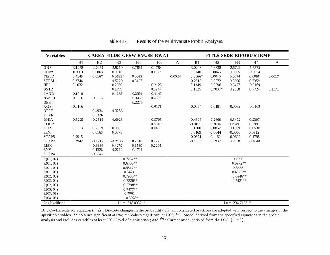
131
Table 4.14. Results of the Multivariate Probit Analysis.
Variables CAREA-FILDB-GRSW-HVUSE-RWAT FITLS-SEDB-RIFOBU-STRMP B1 B2 B3 B4 B5 ∆ B1 B2 B3 B4 ∆
ONE -3.1258 -2.7053 -2.9210 -0.7861 -0.1783 -3.0243 -1.6338 -2.6722 -1.5575 COWS 0.0031 0.0063 0.0010 0.0022 0.0040 0.0045 0.0005 -0.0024 YIELD 0.0145 0.0167 0.0192* 0.0052 0.0024 0.0166* 0.0040 0.0074 0.0058 0.0017 STRM1 0.2744 -0.5220 0.3197 -0.2613 -0.0272 0.2306 0.7359 HEL 0.1032 0.2930 -0.2126 0.1349 -0.0296 0.0477 -0.0169 BSTR 0.1799 0.3247 0.1625 0.7887* 0.2538 0.7724 0.1371 LAND -0.1649 0.4783 -0.2561 -0.4146 NWTH -0.3566 -0.3525 -0.3460 0.4808 DEBT -0.2276 AGE -0.0106 -0.0171 -0.0054 -0.0181 -0.0032 -0.0109 OFFF 0.4934 -0.3253 TOVR 0.3326 DHIA -0.5225 -0.2516 -0.6928 -0.5705 -0.4893 -0.2669 -0.5472 -0.2307 COOP 0.5845 -0.0199 0.2604 0.1949 0.3997 LCES 0.1113 0.2119 0.0965 0.0495 0.1100 0.0862 0.1569 0.0530 SEM 0.0163 0.0578 0.0469 -0.0044 -0.0060 0.0312 SCAP5 0.0915 -0.0371 0.1162 -0.0602 0.1795 SCAP2 0.2942 -0.1715 -0.2186 0.2940 0.2275 -0.1580 0.1937 0.2958 -0.1048 RISK 0.3630 0.4279 0.1589 0.2205 ENV 0.1328 -0.2212 -0.1721 SCAP4 -0.5845 R(01, 02) 0.7252** 0.1990 R(01, 03) 0.6705** 0.6972** R(01, 04) 0.5817** 0.3558 R(01, 05) 0.3424 0.4675** R(02, 03) 0.7905** 0.6646** R(02, 04) 0.7226** 0.7921** R(02, 05) 0.5798** R(03, 04) 0.7477** R(03, 05) 0.3061 R(04, 05) 0.5078* Log likelihood Lu = -318.0332 (a) Lu = -234.7103 (b)
Bi : Coefficients for equation i; ∆ : Discrete changes in the probability that all considered practices are adopted with respect to the changes in the specific variables; ** : Values significant at 5%; * : Values significant at 10%; (a) : Model derived from the specified equations in the probit analysis and includes variables at least 50% level of significance; and (b) : Current model derived from the PCA ( 1)λ = .
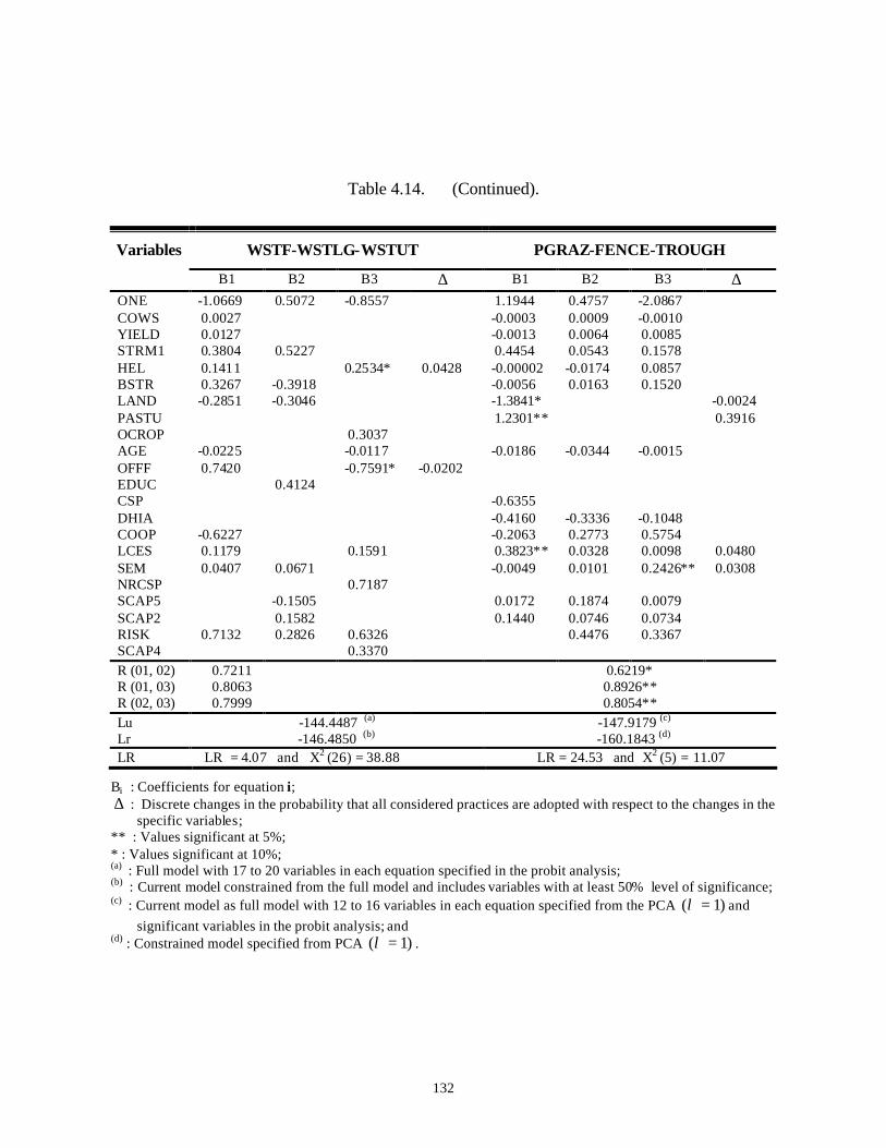
132
Table 4.14. (Continued).
Variables WSTF-WSTLG-WSTUT PGRAZ-FENCE-TROUGH
B1 B2 B3 ∆ B1 B2 B3 ∆ ONE -1.0669 0.5072 -0.8557 1.1944 0.4757 -2.0867 COWS 0.0027 -0.0003 0.0009 -0.0010 YIELD 0.0127 -0.0013 0.0064 0.0085 STRM1 0.3804 0.5227 0.4454 0.0543 0.1578 HEL 0.1411 0.2534* 0.0428 -0.00002 -0.0174 0.0857 BSTR 0.3267 -0.3918 -0.0056 0.0163 0.1520 LAND -0.2851 -0.3046 -1.3841* -0.0024 PASTU 1.2301** 0.3916 OCROP 0.3037 AGE -0.0225 -0.0117 -0.0186 -0.0344 -0.0015 OFFF 0.7420 -0.7591* -0.0202 EDUC 0.4124 CSP -0.6355 DHIA -0.4160 -0.3336 -0.1048 COOP -0.6227 -0.2063 0.2773 0.5754 LCES 0.1179 0.1591 0.3823** 0.0328 0.0098 0.0480 SEM 0.0407 0.0671 -0.0049 0.0101 0.2426** 0.0308 NRCSP 0.7187 SCAP5 -0.1505 0.0172 0.1874 0.0079 SCAP2 0.1582 0.1440 0.0746 0.0734 RISK 0.7132 0.2826 0.6326 0.4476 0.3367 SCAP4 0.3370 R (01, 02) 0.7211 0.6219* R (01, 03) 0.8063 0.8926** R (02, 03) 0.7999 0.8054** Lu -144.4487 (a) -147.9179 (c) Lr -146.4850 (b) -160.1843 (d) LR LR = 4.07 and X2 (26) = 38.88 LR = 24.53 and X2 (5) = 11.07
Bi : Coefficients for equation i; ∆ : Discrete changes in the probability that all considered practices are adopted with respect to the changes in the
specific variables; ** : Values significant at 5%; * : Values significant at 10%; (a) : Full model with 17 to 20 variables in each equation specified in the probit analysis; (b) : Current model constrained from the full model and includes variables with at least 50% level of significance; (c) : Current model as full model with 12 to 16 variables in each equation specified from the PCA ( 1)λ = and
significant variables in the probit analysis; and (d) : Constrained model specified from PCA ( 1)λ = .
133
Since the model in scenario two was nested within that of scenario three, the likelihood
ratio test was conducted to select the appropriate model. The LR value of 27.7 was smaller than
the 2χ critical value; therefore, the constrained model in scenario two was selected. Cow
productivity and business structured as a corporation significantly influenced the adoption of all
four practices. An increase of 100 lbs of milk in the productivity per cow as well as a dairy farm
structured as corporation would increase the probability of adopting all four practices
simultaneously by 0.2 percent and 14 percent, respectively. The second set of models included
three practices. All four estimations associated with the second model resulted in singular
covariance matrices.
4.2.5.2. Wastewater and Runoff Management Practices
Two different sets of models were considered for the group of practices targeting facility
wastewater and runoff management. The first set of models included all practices in the group :
roof runoff management (ROOFR), waste storage facility (WSTF), waste treatment lagoon
(WSTL), and waste utilization (WSTUT). Estimation of the model in scenario two was
successful, but did not yield any significant variables. Estimation of the other three scenarios
resulted in singular covariance matrices. Roof runoff management was left out of the second set
of models, allowing for the examination of the adoption of the three waste management practices
simultaneously. The models in scenario one and four are nested. Therefore, the LR test was
performed to select the appropriate model. Since the LR statistical value of 4.07 was relatively
smaller than the relevant critical value, the constrained model in scenario four was selected. The
higher percentage of farm land classified as “highly erodible” and the holding of an off- farm job
affected the adoption of the three waste management practices simultaneously. A one unit
increase in the percentage of land classified as “highly erodible” would increase the joint
134
adoption of the three waste management practices by 4 percent, and holding an off- farm job
would reduce the probability by 2 percent, holding other variables constant.
4.2.5.3. Grazing Management
Estimation of the multivariate probit model for the three grazing management practices
exhibit the following results: scenarios one and four resulted in singular matrices. The LR test
was performed to select the appropriate model between the two nested models in scenarios two
and three. The LR statistical value of 24.53 was relatively large compared to the relevant
critical value. Therefore, the full model in scenario three was selected. Four variables were
found statistically significant at the 5 and 10 percent levels of significance and included LAND,
PASTU, LCES, and SEM. Each of the variables were associated with similar signs as in the
univariate probit analysis. A one unit increase in the percentage of land owned would decrease
the probability of adopting all three practices by 0.2 percent. The dairy being a pasture-based
operation, one additional meeting with LCES personnel, and attendance at one additional
seminar that dealt with dairy industry issues would raise the probability of adopting all grazing
management practices by 39 , 5 , and 3 percent, respectively.
In summary, the adoption of BMPs by the dairy producer respondents to the survey has
been influenced by the selected variables included in this study. Results of the probit analysis
showed the increased effects of farm size, milk productivity per cow, frequency of meetings
with LCES, and risk aversion. DHIA has consistently been associated with a negative sign.
Results of the bivariate and multivariate probit analyses showed fewer variables which
significantly affected the simultaneous adoption of the practices under consideration.
135
CHAPTER 5
SUMMARY AND CONCLUSIONS
5.1. Summary
Water quality assessments in the U.S. have shown largely improved surface water quality
since the enactment of the Clean Water Act. Even so, efforts to reduce water pollution continue.
These efforts aim to decrease discharges from identifiable sources of water pollution and the
increased contribution of diffused discharges from nonpoint sources. The traditional view of the
agricultural community as a good steward of the environment has been challenged by increasing
concerns about the complex relationship between agricultural production activities and
environmental quality. Along with its positive contribution of providing a wide range of
products to satisfy human needs, agriculture has also been blamed for contributing to
environmental problems. The significant role of agriculture as a major source of water pollution
has been pointed out.
Recent environmental policy has focused on reducing water pollution produced by
agriculture. Different programs have been undertaken at the Federal and State levels to address
agricultural point and nonpoint sources of pollution, and agricultural producers are encouraged to
voluntarily implement site specific management practices known as best management practices
(BMPs). These practices consist of conservation methods designed to reduce the delivery and
transport of agriculturally derived pollutants such as sediment, nutrients, pesticides, salt and
pathogens to surface and ground waters.
Louisiana is far from being a major U.S. milk producer. However, the dairy industry
represents one of the most important animal agricultural industries in the state. Similar to other
agricultural production activities, the need to adopt specific practices to improve water quality

136
has become greater in the dairy industry as dairy farms in the Florida parishes have been targeted
in recent years as polluters of waterways.
This study investigated the adoption of 21 BMPs aimed at reducing the impact of dairy
farming on Louisiana’s environment. Specific objectives of the study were to: examine the
current efforts to contain water quality degradation, including regulatory measures, research and
educational programs on environmental issues as they relate to Louisiana dairy industry; review
the literature on technology adoption in the agricultural sector; assess the extent of current
adoption of BMPs in the Louisiana dairy industry; determine the effects of demographic,
socioeconomic and farm characteristics on producers’ decisions to adopt specific BMPs; and
make policy recommendations based on the empirical results.
Federal and state actions aiming at the improvement of national water quality have been
continual over the years. Current programs include the pursuit of existing long-term programs
initiated over fifty years ago as well as recent programs established to address specific issues.
The protection, conservation and restoration of natural resources in Louisiana has involved the
Natural Resources and Conservation Service (NRCS) through local soil and conservation
districts, conservation development areas, landowners and partners and volunteers. Current
conservation programs in Louisiana include but are not limited to: the Environmental Quality
Incentives Program (EQIP), which assists eligible farmers and ranchers in complying with
federal, state and tribal environmental laws through cost-sharing to implement BMPs; the
Louisiana Grazing Lands Conservation Initiative (GLCI), which provides financial and technical
assistance to owners and managers of pastureland, rangeland, grazed woodlands, and potentially
grazed cropland, and promotes voluntary adoption of prescribed grazing practices by livestock
producers; and the Conservation Reserve Program (CRP), which assists producers in retiring
137
highly erodible and environmentally sensitive croplands for 10 to 15 years by paying producers
an annual “rental fee” upon entering the program.
The study of technology adoption has retained researchers’ interests over the years since
Griliches’ exploration of the wide differences in the rate of adoption of hybrid seed corn in 1957.
Selected literature of relevance to this study were reviewed to provide insights of previous
findings regarding agricultural producers’ adoption of technology. Technologies ranged from
those that increase production efficiency to those whose sole purpose is to reduce environmental
damages associated with production activities. These studies investigated the likely determinants
of agricultural producers’ decisions to adopt a specific technology and used different theoretical
models of adoption. Studies on environmental attitude have shown the wide-spread use of the
New Environmental Paradigm (NEP) scale, developed by Dunlap et al. in 1978, and revised in
2000, as a measure of environmental attitude.
A mail survey of the population of dairy producers (428), designed according to
Dillman’s method of surveying, was conducted in Summer, 2001, to provide data for the
analysis. It included a first mailing, followed by a postcard reminder, and a second mailing to
non-respondents. One hundred and thirty one surveys were returned with 124 completed,
achieving an effective rate of return of 29 percent.
The sample was comprised mostly of pasture-based operations located in the southeastern
region of Louisiana, specifically in St. Helena, Tangipahoa and Washington parishes. Ninety
percent of the farms were producing at least at the state average milk production per cow of
12,155 pounds in 2000. The survey respondents were mostly male producers, between 40 and 59
years old, with a high school diploma or a bachelor’s degree. A large number of respondents
were not aware of the Coastal Nonpoint Control Program, nor the effort to control water
138
pollution through the Clean Water Act. Producers who had heard about BMPs for dairy had
received the information primarily from the LCES, government agencies such as NRCS, and
farm organizations such as the Farm Bureau.
Elicitation of dairy producers’ attitudes toward the environment was conducted using the
NEP scale developed by Dunlap et al. in 2000. Results showed an average score of 3.22,
suggesting a tendency of dairy producers to hold, on average, a neutral attitude regarding the
issues stated in the 15 items of the NEP scale.
Different rates of adoption were found for each BMP. Non-adoption was due mainly to a
need for more information or the real or perceived non applicability of the specific practice to the
farm. The group of practices targeting erosion and sediment control had the lowest rates of
adoption, varying from 28 percent (for streambank and shoreline protection) to 48 percent (for
field borders), except for conservation tillage, which was adopted by 77 percent of the
respondents. The low rates might be due to producers’ adoption of BMPs according to their
primary activities. The adoption of practices related to erosion and sediment reduction could be
secondary in the eyes of the dairy producers. Practices aiming at the management of facility
wastewater recorded the highest rates of adoption among all BMPs. The adoption rates vary
from 70 percent (for waste storage facility) to 83 percent (for waste management system). These
practices have been emphasized greatly by NRCS in recent years. The adoption of nutrient and
pesticide management were 69 and 62 percent, respectively. Survey results suggest that about 10
percent of the producers had not heard about these two BMPs, 11 percent of the respondents
considered nutrient management not applicable to their farms and 23 percent thought the same
regarding pesticide management. The three grazing management practices had high rates of
adoption: 80 percent for fencing; 72 percent for grazing management ; and 70 percent for trough
139
or tank. The pasture-based operation type of most respondents’ dairies expla ins these rates of
adoption of grazing management practices.
However, these adoption rates, based on the total respondents, might be understated
given the relatively high rates of “non applicability” responses. The true adoption rates
regarding the practices targeting erosion and sediment control might be higher than those
actually provided when accounting only for dairy farms that should apply the BMP. This is
consistent with the site specific characteristic of BMPs. The adoption rate will go up if the
denominator accounts for a smaller number of producers that should adopt the BMP. On the
other hand, as Donny Latiolais suggested, there might be producers who already implemented
the practice but failed to recognize the BMP despite the short glossary provided in the survey. In
such a case, the numerator of the ratio, accounting for the total number of producers adopting the
BMP would be higher, and so would be the percentage of adoption.
A second limitation in interpreting these numbers as representative is that the average
milk yield of the surveyed farmers, 14,984 pounds, was higher than the average Louisiana dairy
farm milk yield, 12,155 pounds in 2000. Since higher yielding producers were generally the
more extensive adopters, these adoption rates may be overstated. However, the differences may
not be great, given the relatively small marginal effects of YIELD on the probability to adopt,
ranging from 0.02 to 0.08 percent for each additional 100 pounds in milk production per cow.
Producers’ decisions regarding whether to adopt a specific BMP were investigated
through probit analysis. The simultaneous adoption of two or more BMPs was examined using
bivariate and multivariate probit models, assuming contemporaneous errors between adoption
equations. Thirty two variables were hypothesized as relevant in determining dairy producers’
decisions to adopt BMPs, and descriptive statistics of these variables were provided.
140
Collinearity diagnostic s revealed four variables were strongly correlated. Thus, variables
accounting for social relationships with neighboring farmers (SCAP1) and other agricultural
businesses (SCAP3) were assessed as less important in the decision process and were excluded
from the set of explanatory variables to reduce the collinearity problem. The conduct of
principal component analysis (PCA) allowed for reducing the number of variables from 30 to 17
(with 0.7λ = ) and 12 (with 1λ = ) needed for the multivariate probit analysis.
Four different probit models were run for each BMP: a base model with 30 variables; a
second model with the 17 variables retained from the PCA procedure; a third model as an
extension of model two, with extra variables from the base model that were significant at the 10
percent level; and a fourth model with variables from the base model that were significant at the
50 percent level. All Lagrange multiplier statistic values had large p-values, suggesting
homoskedastic error terms associated with each adoption equation. The values of McFadden and
Estrella R2 statistics were relatively low, about 0.20, except for the waste management system
(0.50) and prescribed grazing (0.40) equations. Estimates of the Akaike Information Criterion
(AIC) and the Schwartz Criterion (SC), as well as the conduct of the likelihood ratio test allowed
for selection of the best model to be considered in the multivariate analysis. The marginal
effects of continuous explanatory variables were assessed at mean values of all variables as well
as at selected values of the dummy variables. Discrete changes in the predicted probabilities
were estimated as an alternative to marginal effects in the case of dummy variables.
Results from the probit models suggest that farm size (COWS), milk productivity
(YIELD), frequency of meetings with LCES personnel (LCES), and risk aversion (RISK) were
associated with significant increases in the adoption of 5 to 8 specific BMPs. Nine variables
were found significantly associated with increased adoption of 1 to 3 specific BMPs. These
141
variables include: having a stream running through the farm land (STRM1), percentage of land
classified as “highly erodible” (HEL), business structured as a corporation (BSTR), dairy farm
net worth (NWTH), the holding of an off- farm job (OFFF), farmer’s educational attainment
(EDUC), having a family member planning to take over the dairy operation upon the producer’s
retirement (TOVR), membership in a milk cooperative (COOP), and good relationships with
lending institutions (SCAP2).
Variable AGE frequently had a negative sign, which was as expected. Older producers
would be expected to have shorter planning horizons and would be less willing to alter their
management strategies. The consistent negative association between membership in DHIA and
BMP adoption was not as expected. In this study, better record keepers, likely to be the more
progressive farmers, were hypothesized to be more willing to adopt conservation practices. The
negative correlation could be because of DHIA targeting dairy farm productivity and ensuring
higher profit through highly monitored business management. Conservation practices, on the
other hand, primarily target an overall improvement of the environment, which may ensure long
term financial viability, but may not result in greater short-run profit.
Dairy producers most likely to adopt BMPs were more likely to be operating larger farms
with greater milk productivity per cow. These producers were also more highly educated and
risk averse. The significant influence of meetings with LCES personnel suggests the importance
of information dissemination in inducing adoption of BMPs, and the effectiveness of LCES at
influencing adoption.
The adoption of two BMPs simultaneously was examined using bivariate probit analysis,
based on the selected models from the probit analysis of each BMP. The group of practices
aiming at erosion and sediment control was divided into two subcategories according to whether
142
they target primarily erosion reduction or sediment control. Thirty-eight bivariate probit models
were analyzed in total: 21 for the seven practices in the subgroup of practices targeting the
reduction of soil erosion; six for the group of practices aiming at sediment control; seven for the
group of practices dealing with facility and wastewater and runoff management; one for nutrient
and pesticide management; and three for the grazing management practices.
Thirty-two of the rho coefficients were found statistically significant at the 5 or 10
percent levels of significance, suggesting simultaneity in the adoption of BMPs. Conditional
marginal effects associated with the bivariate model were provided. Models associated with the
group of practices targeting erosion and sediment control tended to heavily predict the adoption
of neither practice under consideration, probably due to the low rate of adoption of most
practices in the group.
Compared with the univariate probit analyses, fewer variables were found to significantly
influence the simultaneous adoption of two practices. The holding of an off- farm job, plans for a
family member to take over the dairy operation upon the farmer’s retirement, frequency of
meetings with LCES personnel and good relationships with non-farmer neighbors were
associated with greater adoption of field borders given that grassed waterways had been adopted.
Larger percentages of farm land classified as “highly erodible” and a good relationship with non-
farmer neighbors would increase the adoption of grassed waterways provided that field borders
had been established.
The holding of an off- farm job was the only variable that had a significant positive effect
on the implementation of both a waste storage facility and waste utilization practices. Off- farm
income allow producers to overcome the capital constraint associated with the implementation of
somewhat capital intensive practices such as the construction of pound for waste storage.
143
Membership in DHIA would reduce the implementation of nutrient management if producers
had adopted pesticide management. Having a stream and/or river running through the farm
would increase the adoption of pesticide management by producers with a nutrient management
plan. Meeting with LCES personnel would increase the establishment of a prescribed grazing
plan if dairy farmers had their land fenced, but a larger percentage of land owned to total acres of
land included in the operation would reduce the adoption.
The simultaneous adoption of larger sets of three to six BMPs in each group of practices
was investigated. Four different scenarios were examined regarding the variables to be included
in the system of 3 to 6 equations in the multivariate probit analysis. Models in the first scenario
included variables from the selected probit models. Models in scenario two included the 12
variables obtained from the PCA ( 1)λ = in each of the equations. Models in scenario three, as
extensions of the models in scenario two, included some extra variables from the probit models
that were significant at the 10 percent level. Models in scenario four included variables from the
probit models that were significant at the 50 percent level of significance. Two sets of models
were considered for each group of practices. Discrete changes in the probability of adopting all
practices under consideration were estimated as alternatives to marginal effects. Fewer variables
were significant as more equations were considered in the multivariate probit analysis. Dairy
farms with higher milk productivity were likely to simultaneously implement the five practices
targeting erosion reduction including critical area planting, field borders, grassed waterways,
heavy use area protection and regulating water in a drainage system. Milk productivity and
business structured as a corporation would enhance the adoption of four sediment control
practices such as filter strips, sediment basin, riparian forest buffer and streambank and shoreline
protection. A higher percentage of farmland classified as “highly erodible” and the holding of an
144
off- farm job likely increased the adoption of waste facilities, a lagoon and proper waste
utilization. Pasture-based operations and diversification of farming activities would enhance
producers’ implementation of the three grazing management practices.
5.2. Conclusions and Recommendations
This study showed that the adoption of BMPs by Louisiana dairy producers was
influenced by factors such as farm characteristics, operator characteristics, institutions related to
the dairy operation, and producers attitude. Results of the analysis emphasized:
• The positive influence of farm size on the adoption of BMPs that are not particularly
capital- intensive in nature such as conservation tillage, critical area planting, field
borders and filter strips. Such practices are unlikely to require substantial initial
capital investment and economies associated with spreading associated fixed costs
over greater output are not likely to be substantial in most cases. The rationale for
such results would be the possibility of larger farms appropriating the learning costs
as fixed expenses, as suggested by Feder et al. (1985);
• The effect of milk productivity per cow on the increased adoption of BMPs such as
cover and green manure crops, establishment of field borders, filter strips, grassed
waterways, waste storage facility, and nutrient management. Higher milk
productivity is indicative of a well-managed farm. Although BMPs do not
necessarily affect milk productivity in the short-run, better managers are likely to
adopt practices that ensure the long-run viability of their operations. In the case of
the waste storage facility, substantial initial investment is likely to be required. More
productive farms will more likely be better able to bear the fixed adoption costs
associated with such a facility;
145
• The increased effect of frequent meetings with LCES personnel on the adoption of
eight BMPs including conservation tillage, the establishment of field borders, grassed
waterways, riparian forest buffers, the construction of a waste storage facility, proper
utilization of wastes, a nutrient management plan, and prescribed grazing. These
results underscore the importance of information dissemination in inducing adoption
and the effectiveness of LCES in providing BMP information to producers;
• The influence of producer’s risk aversion on the adoption of six of the more capital
intensive BMPs. These practices included the establishment of grassed waterways,
the construction of a sediment basin, streambank and shoreline protection, waste
storage facilities, proper utilization of waste and fencing. Adoption of such BMPs
helps to ensure long-run economic viability of the land and avoidance of the risk
associa ted with decreased productivity resulting from unusually heavy rainfall events;
• The consistent negative effect of membership in DHIA on the adoption of nine
somewhat capital intensive BMPs including critical area planting, filter strips, grassed
waterways, regulating water in a drainage system, riparian forest buffers, sediment
basins, streambank and shoreline protection, and waste storage facility. DHIA allows
for enhancing dairy operation productivity and ensuring higher profit through an
extensive record keeping system. The negative effect of DHIA suggests that the
adoption of BMPs might not be consistent with the goals of producers who place
greater weight on the profit-maximization goal, as opposed to other goals such as
conserving and maintaining land. These producers may require greater economic
incentives to induce adoption, offered through extended cost-sharing programs or
programs that provide financial assistance for maintenance of BMPs;
146
• The lower probability that older producers had adopted BMPs that required
substantial initial capital investments such as sediment basins, waste storage facilities,
and fencing. Such investments are unlikely to be made by producers with short
planning horizons since the producer cannot benefit from the full stream of benefits,
but must absorb the full costs;
• The result that producers with highly erodible land or streams running through their
farms, land characteristics that place a farm at particular risk of polluting water, were
more likely to adopt several practices. Grassed waterways and waste utilization were
used more by producers with highly erodible land. These are BMPs that can address
runoff concerns if utilized properly. Streambank and shoreline protection was
utilized, not surprisingly, by those who had streams running through their land.
These results likely show the effectiveness of educational programs at targeting high
risk polluters for adoption, and the benefits such producers recognize from adoption;
and
• The greater likelihood of more highly educated producers to adopt streambank and
shoreline protection, waste management systems, waste treatment lagoons and
pesticide management. Higher educational attainment allows farmers not only
greater access to information, but also recognition of the benefits and costs of
alternative management strategies such as adopting BMPs. More educated producers
may have more ability to adjust to changes.
The relatively high rates of adoption of facility wastewater management practices as well
as those related to grazing management indicate that most dairy producers have established these
practices. However, the overall findings suggest the need to address the following points:
147
• The lack of knowledge among dairy producers about BMPs. This is reflected by the
large number of producers unaware of legislation and efforts to control nonpoint
sources of water pollution, as well as the high rates of respondents answering “need
more information” and “have not heard about it” as reasons for not adopting a BMP;
• The low rate of producers having a dairy farm plan with NRCS; and
• The need of expanded economic incentives to induce the adoption of producers who
find a BMP too expensive to adopt, or are short-run profit maximizers.
The lack of information can be addressed through intensive educational programs to
inform producers about BMPs such as the Louisiana Master Farmer Program. This program, co-
sponsored by the LSU Agricultural Center and other groups, puts primary emphasis on educating
Louisiana farmers about BMPs in a three-year program of study. The statewide educational
program intends to cover the 12 watersheds in Louisiana over the next five years. Along with
the educational program, it is also important to encourage dairy producers to establish a dairy
farm plan with NRCS, which would allow for specifying the BMPs applicable to the dairy farm.
The need of economic incentives can be addressed through the technical and financial
assistance promoted by EQIP. EQIP targets primarily (60 percent) livestock operations and
supplies up to a 75 percent cost-share (90 percent for beginning farmers and ranchers) for
implement ing conservation practices. This program increases the profitability associated with
BMPs, thereby inducing producers who place greater emphasis on the profit-maximization goal
to adopt.
Lastly, the conduct of programs that assist producers in maintaining established BMPs
would be necessary to ensure sustained improvement in the environment. Indeed, the recurrent
expenses associated with the operation and maintenance of established BMPs could be costly to
148
the farm operation. The Conservation Security Program (CSP), established under the 2002 Farm
Bill, constitutes a national incentive payment program to assist agricultural producers in adopting
and maintaining new conservation measures related to the management of land. Provisions list
management practices as including but not limited to nutrient management, integrated pest
management, grazing management, controlled rotational grazing, and soil conservation and
residue management. Unfortunately, the program does not cover already established
conservation practices. However, it might be a motivating factor for current non-adopters of
BMPs for targeting erosion and sediment control.
The findings of this study pointed out, among others things, the importance of economic
incentives in producers’ decisions to adopt. However, this study did not provide insights
regarding the extent of such incentives to induce BMP adoption nor the likely profitability of
BMPs. Therefore, a thorough investigation of producers’ willingness to adopt BMPs provided
that economic incentives are available would allow for ascertaining the likely positive
association between BMP adoption and economic incentives. Given that few estimates are
available as to the costs associated with BMP adoption, further research may also examine the
true profitability of a BMP to a farm and provide agricultural producers a better understanding of
how BMPs impact not only the environment but also the economic viability of their operation.
149
REFERENCES
1998 Louisiana Agricultural Statistics. Louisiana State University Agricultural Center. Department of Agricultural Economics and Agribusiness. A.E.A. Information Series No. 177. October 1999.
2000 Louisiana Agricultural Statistics. Louisiana State University Agricultural Center.
Department of Agricultural Economics and Agribusiness. A.E.A. Information Series No. 195. September 2001.
Albrecht, Stan L. and Kerry E. Carpenter. “Attitudes as Predictors of Behavior versus Behavior
Intentions: A Convergence of Research Traditions.” Sociometry. 39 (1976): 1-10. Anderson, Jock R. “The Economics of New Technology Adaptation and Adoption.” Review of
Marketing and Agricultural Economics. 61 (August 1993): 301-309. Anderson, Jock R. and John Dillon. “Risk Analysis in Dryland Farming Systems.” Farm
Systems Management Series No. 2. Food and Agriculture Organization of the United Nations. Rome. 1992.
Arcury, Thomas and Eric H. Christianson. “Environmental Worldview in Response to
Environmental Problems – Kentucky 1984 and 1988 Compared.” Environment and Behavior. 22 (May 1990): 387-407.
Arcury, Thomas. “Environmental Attitude and Environmental Knowledge.” Human
Organization. 49 (1990): 300-304. Barbier, Edward B. “The Farm-Level Economics of Soil Conservation: The Uplands of Java.”
Land Economics. 66 (May 1990): 199-211. Basilevsky, Alexander. “Statistical Factor Analysis and Related Methods. Theory and
Applications.” Wiley Series in Probability and Mathematical Statistics. John Wiley & Sons, Inc. New York. 1994.
Bebbington, Anthony. “Social Capital and Rural Intensification: Local Organizations and
Islands of Sustainability in the Rural Andes.” The Geographical Journal. 163 (July 1997): 189-97.
Börsch-Supan, Axel and Vassilis A. Hajivassiliou. “Smooth Unbiased Multivariate Probability
Simulators for Maximum Likelihood Estimation of Limited Dependent Variable Models.” Journal of Econometrics. 58 (August 1993): 347-68.
Bourdieu, Pierre. “Forms of Capital.” Handbook of Theory and Research for the Sociology of
Education. John G. Richardson. Greenwood Press. New York. 1983.
150
Brehm, John. “Individual-Level Evidence for the Causes and Consequences of Social Capital.” American Journal of Political Science. 41 (July 1997): 999-1023.
Burt, Ronald S. “The Contingent Value of Social Capital.” Administrative Science Quarterly.
42 (June 1997): 339-65. Cardona, Hugo. “Analysis of Policy Alternatives in the Implementation of Coastal Nonpoint
Pollution Control Program for Agriculture.” Unpublished PhD. Dissertation. Louisiana State University. Department of Agricultural Economics and Agribusiness. 1999.
Case, Karl E and Ray C. Fair. Principles of Microeconomics. 2nd Ed. Prentice Hall, Inc.
Englewood Cliffs, New Jersey. 1992. Caswell, Margriet and David Zilberman. “The Choices of Irrigation Technologies in
California.” American Journal of Agricultural Economics. 67 (May 1985): 224-234. Chai, Sun-Ki. Choosing an Identity: A General Model of Preference and Belief Formation. The
University of Michigan Press. Ann Arbor. USA. 2001. Coase, R. H. “The Problem of Social Cost.” Journal of Law and Economics. 3 (1960): 1-44. Coleman, James S. “Social Capital in the Creation of Human Capital.” American Journal of
Sociology. 94 (1988): S95-S120. Cooper, Joseph C. “A Joint Framework for Analysis of Agri-Environmental Payment
Programs.” Paper presented at the Annual Meetings of the American Agricultural Economics Association, Chicago, Illinois, August 5-8, 2001.
Daultrey, S. “Principal Component Analysis.” Concepts and Techniques in Modern
Geography. No. 8. Geo Abstracts. University of East Anglia, Norwich. 1976. Davis, Christopher G. and Jeffrey M. Gillespie. “Technology Adoption in U.S. Hog
Production.” Paper presented at the Annual Meetings of the Southern Agricultural Economics Association, Fort Worth Texas, January 28-31, 2000.
Dillman, Don A. “The Design and Administration of Mail Surveys.” Annual Review of
Sociology. 17 (1991): 225-49. ______________. Mail and Telephone Surveys: The Total Design Method. Wiley. New York.
1978. Dorfman, Jeffrey H. “Modeling Multiple Adoption Decisions in a Joint Framework.” American
Journal of Agricultural Economics. 78 (August 1996): 547-57.
151
Drapcho, Caye M., James F. Beatty and Eric C. Achberger. “Water Quality and the Tangipahoa River.” Louisiana Agriculture: The Magazine of the Louisiana Agricultural Experiment Station. 44 (Spring 2001): 16-17.
Dunlap, Riley E. and Kent D. Van Liere. “The New Environmental Paradigm: A Proposed
Measuring Instrument and Preliminary Results.” Journal of Environmental Education. 9 (1978): 10-19.
Dunlap, Riley E., Kent D. Van Liere, Angela G. Mertig, and Robert E. Jones. “Measuring
Endorsement of the New Ecological Paradigm: A Revised NEP Scale.” Journal of Social Issues. 56 (Fall 2000): 425-42.
El-Osta, Hisham S. and Mitchell J. Morehart. “Technology Adoption Decisions in Dairy
Production and the Role of the Herd Expansion. ” Agricultural and Resource Economics Review. 28 (April 1999): 84-95.
Environmental Protection Agency. National Water Quality Inventory: 1998 Report to
Congress. EPA841-R-00-001. 1998. (http://www.epa.gov/305b/98report/). _____________________________. A Phase I Inventory of Current EPA Efforts to Protect
Ecosystems. Tangipahoa River. 1995. (http://www.epa.gov/ecoplaces/part2/region6/site10.html) _____________________________. Office of Water. Guidance Specifying Management
Measures for Sources of Nonpoint Pollution in Coastal Waters. EPA-840-B-93-001C. January 1993.
_____________________________. Office of Water. Guidance Specifying Management
Measures for Sources of Nonpoint Pollution in Coastal Waters. EPA-840-B-93-001C. Revised January 1997.
(http://www.epa.gov/OWOW/NPS/MMGI/index.html) _____________________________. Office of Water. National Management Measures to
Control Nonpoint Source Pollution from Agriculture. EPA-68-C99-249. August 2000(a). (http://www.epa.gov/OWOW/NPS/AGMM/index.html)
_____________________________. Office of Wastewater Management. Guidance Manual
and Sample NPDES Permit for Concentrated Animal Feeding Operations. Final Internal Review Draft. September 2000(b).
(http://www.epa.gov/npdes/pubs/dman_afo-2000.pdf) Estrella, Arturo. “A New Measure of Fit for Equations with Dichotomous Dependent
Variables.” Journal of Business and Economic Statistics. 16 (April 1998): 198-205.
152
Fausti, S. W. and J. M. Gillespie. “A Comparative Analysis of Risk Preference Elicitation Procedures Using Mail Survey Results.” Presented at SERA-IEG-31 Meeting, Gulf Shores, Alabama. March 23-25, 2000.
Feder, Gershon, Richard E. Just, and David Zilberman. Adoption of Agricultural Innovations in
Developing Countries. A Survey. World Bank Staff Working Paper No. 542. Washington, DC. USA. 1985.
Fernandez-Cornejo, Jorge, E. Douglas Beach, and Wen-Yuan Huang. “The Adoption of IPM
Techniques by Vegetable Growers in Florida, Michigan and Texas.” Journal of Agricultural and Applied Economics. 26 (July 1994): 158-72.
Fleisher, Beverly. Agricultural Risk Management. Lynne Rienner Publishers, Boulder &
London. Boulder, Colorado. USA. 1990. Fomby, Thomas B., R. Carter Hill and Stanley R. Johnson. Advanced Econometric Methods.
Springer-Verlag New York Inc. New York. 1984. Freda, Jon S. and Joyce L. Shields. “An Investigation of the Adoption Process in Training
Technology Transfer.” U.S. Army Research Institute for the Behavioral and Social Sciences. Technical Report 448. June 1980.
Friedman, Debra and Michael Hechter. “The Contribution of Rational Choice Theory to
Macrosociological Research”. Sociology Theory. 6 (Fall 1988): 201-18. Geweke, John. “Bayesian Inference in Econometric Models Using Monte Carlo Integration.”
Econmetrica. 57 (November 1989): 1317-39. Ghosh, Soumen, J. T. McGuckin, and S. C. Kumbhakar. “ Technical Efficiency, Risk Attitude,
and Adoption of New Technology: The Case of the U.S. Dairy Industry.” Technological Forecasting and Social Change. 46 (July 1994): 269-78.
Gould, Brian W., William E. Saupe, and Richard M. Klemme. “Conservation Tillage: The Role
of Farm and Operator Characteristics and the Perception of Soil Erosion.” Land Economics. 65 (May 1989): 167-182.
Govindasamy, Ramu and Mark J. Cochran. “ The Conservation Compliance Program and Best
Management Practices: An Integrated Approach for Economic Analysis.” Review of Agricultural Economics. 17 (1995): 369-381.
Grant, Emma. “Social Capital and Community Strategies: Neighbourhood Development in
Guatemala City.” Development and Change. 32 (2001): 975-97. Greene, William H. Econometric Analysis. Fourth Edition. Prentice Hall, Inc. Upper Saddle
River, New Jersey. 2000.
153
Griliches, Zvi. “Hybrid Corn: An Exploration in the Economics of Technological Change.” Econometrica. 25 (October 1957): 501-522.
Gürler, Ülkü and Kathryn Prewitt. “Bivariate Density Estimation with Randomly Truncated
Data.” Journal of Multivariate Analysis. 74 (2000): 88-115. Gürler, Ülkü. “Bivariate Distribution and Hazard Functions when a Component is Randomly
Truncated.” Journal of Multivariate Analysis. 60 (1997): 20-47. Hair, Joseph F., Rolph E. Anderson, Ronald L. Nathan, and William C. Black. Multivariate
Data Analysis. Fifth Edition. Prentice Hall Inc. Upper Saddle River, New Jersey. 1998. Heath, Anthony. Rational Choice & Social Exchange: A Critic of Exchange Theory.
Cambridge University Press. New York. 1976. Henderson, James H. and Richard E. Quandt. “Microeconomic Theory: A Mathematical
Approach.” 3rd Ed. Economics Handbook Series. McGraw-Hill, Inc. New York. 1980. Hutcheson, Graeme D. and Nick Sofroniou. The Multivariate Social Scientist. Sage
Publications Ltd, London. 1999. Intriligator, Michael D., Ronald G. Bodkin, and Cheng Hsiao. Econometric Models,
Techniques, and Applications. 2nd Ed. Prentice Hall, Inc. Upper Saddle River, New Jersey. 1996.
Ipe, Viju C., Eric A. DeVuyst, John B. Braden and David C. White. “Simulation of a Group
Incentive Program for Farmer Adoption of Best Management Practices.” Agricultural and Resource Economics Review. 30 (October 2001): 139-150.
Isebrands, J. G. and Thomas R. Crow. Introduction to Uses and Interpretation of Principal
Component Analysis in Forest Biology. USDA Forest Service General Technical Report NC-17. North Central Forest Experiment Station. St. Paul, Minnesota. 1975.
Jolliffe, L. T. “Discarding Variables in a Principal Component Analysis. I: Artificial Data.”
Applied Statistics. 21 (1972): 160-173. ___________. “Discarding Variables in a Principal Component Analysis. II: Real Data.”
Applied Statistics. 22 (1973): 21-31. Jones, Robert Emmet and Riley E. Dunlap. “ The Social Bases of Environmental Concern:
Have They Changed Over Time?” Rural Sociology. 57 (1992): 28-47. Judge, G. G., R. C. Hill, W. E. Griffiths, H. Lütkepohl, and T. Lee. Introduction to the Theory
and Practice of Econometrics. 2nd Edition. John Wiley & Sons, Inc. New York. 1988.
154
Judge, G. G., W. E. Griffiths, R. C. Hill, H. Lütkepohl, and T. Lee. “The Theory and Practice of Econometrics.” 2nd Edition. Wiley Series in Probability and Mathematical Statistics. John Wiley & Sons, Inc. New York. 1985.
Kahn, James R. The Economic Approach to Environmental and Natural Resources. 2nd Ed. The
Dryden Press. Harcourt Brace College Publishers. New York. 1998. Keane, Michael P. “A Computationally Practical Simulation Estimator for Panel Data.”
Econometrica. 62 (January 1994): 95-116. Keeney, Ralph L. and Howard Raiffa. Decisions with Multiple Objectives: Preferences and
Value Tradeoffs. Cambridge University Press. New York. 1993. King, R. P. and L. J. Robison. “An Interval Approach to the Measure of Decision Maker
Preferences.” American Journal of Agricultural Economics. 63 (1981): 510-20. Knutson, Ronald D., J. B. Penn, and Barry L. Flinchbaugh. Agricultural and Food Policy. 4th
Edition. Prentice Hall. Upper Saddle River, New Jersey. 1998. Krause, Mark A. and J. Roy Black. “ Optimal Adoption Strategies for No-Till Technology in
Michigan.” Review of Agricultural Economics. 17 (September 1995): 299-310. Lichtenberg, Erik. “Agriculture and the Environment.” University of Maryland. Department of
Agricultural and Resource Economics. Working Paper No. 00-15. September 2000. Lim-Applegate, Hazel, Gil Rodriguez and Rose Olfert. “Determinants of Non-Farm Labour
Participation Rates Among Farmers in Australia.” The Australian Journal of Agricultural and Resource Economics. 46 (2002): 85-98.
Long, Scott J. “Regression Models for Categorical and Limited Dependent Variables.”
Advanced Quantitative Techniques in Social Sciences Series. Sage Publications, Inc. Thousand Oaks, California. 1997.
Louisiana State Department of Health and Human Resources. Office of Health Services and
Environmental Quality. Reports prepared by the Milk and Dairy Division (1981 through 2000).
Louisiana State University Agricultural Center. Dairy Production Best Management Practices
(BMPs). Pub. 2823. 2000. Lynne, Gary D. “Modifying the Neo-Classical Approach to Technology Adoption with
Behavioral Science Models.” Journal of Agricultural and Applied Economics. 27 (July 1995): 67-80.
Machina, Mark J. “Choice Under Uncertainty: Problems Solved and Unsolved.” Journal of
Economic Perspectives. 1 (Summer 1987): 121-54.
155
Marbery, Steve. “Citizens Sue EPA and Land O’Lakes, Inc.” Feedstuffs. March 18, 1996. McCloskey, Donald N. “The Economics of Choice. Neoclassical Supply and Demand.”
Economics and the Historian. University of California Press. Berkeley and Los Angeles. 1996.
McFadden, D. “Conditional Logit Analysis of Qualitative Choice Behavior.” Frontiers in
Econometrics. Editor P. Zarembka. Academic Press, New York. 1973. Miller, Roger Leroy. Economics Today: The Micro View. 8th Ed. HarperCollins College
Publishers. New York. 1994 Moser, M. Christine and Christopher B. Barrett. “The Complex Dynamics of Smallholder
Technology Adoption: The Case of SRI in Madagascar.” Paper presented at the AAEA-WAEA Annual Meeting, Long Beach California, July 28-31, 2002.
Mueller, Daniel J. Measuring Social Attitude. A Handbook for Researchers and Practitioners.
Teachers College Press. Columbia University. New York. 1986. Natural Resources Conservation Service. Farm Bill 2002. Environmental Quality Incentives
Program. Key Points. June 2002. (http://www.usda.gov/farmbill/conference_report/title2.pdf) Nunnally, Jum C. and Ira H. Bernstein. Psychometric Theory. 3rd Ed. McGraw-Hill, Inc. 1994. Pakes, Ariel and David Pollard. “Simulation and the Asymptotics of Optimization Estimators.”
Econometrica. 57 (September 1989): 1027-57. Parkin, Michael. “Microeconomics.” 3rd Ed. Updated Edition. The Addison–Wesley Series in
Economics. Addison Wesley Longman Inc. New York. 1997. Paxton, Pamela. “Is Social Capital Declining in the United States? A Multiple Indicator
Assessment.” American Journal of Sociology. 105 (July 1999): 88-127. Peterson, H. Christopher, Lindon Robison, and Marcelo E. Siles. “The Social Capital
Foundations of Trust in Global Agri-Food System Transactions.” Staff Paper No. 99-19. Department of Agricultural Economics, Michigan State University. June 1999.
Pierce, John C., Nicholas P. Lovrich, Jr., Taketsugu Tsurutani, and Takematsu Abe. “
Environmental Belief Systems Among Japanese and American Elites and Publics.” Political Behavior. 9 (1987): 139-159.
Pigou, A. C. The Economics of Welfare. MacMillan and Company, London. 1938. Putman, Robert P. “Bowling Alone: America’s Declining Social Capital.” Journal of
Democracy. 6 (1995): 65-78.
156
Randall, Allan. Resources Economics: An Economic Approach to Natural Resource and Environmental Policy. 2nd Edition. John Wiley & Sons. New York. 1987.
Rahelizatovo, Noro C. and Jeffrey M. Gillespie. “Dairy Farm Size, Entry, and Exit in a
Declining Production Region.” Journal of Agricultural and Applied Economics. 31 (August 1999): 333-47.
Rao, C. R. “The Use and Interpretation of Principal Component Analysis in Applied Research.”
Sankhya: The Indian Journal of Statistics: Series A. 26 (1964): 329-358. Reinhard, Stijn, C. A. Knox Lovell, and Geert Thijssen. “Econometric Estimation of Technical
and Environmental Efficiency: An Application to Dutch Dairy Farms.” American Journal of Agricultural Economics. 81 (February 1999): 44-60.
Ribaudo, Marc O., Richard D. Horan, and Mark E. Smith. Economics of Water Quality
Protection From Nonpoint Sources: Theory and Practice. USDA-ERS Agricultural Economic Report. No. 782. November 1999.
Rule, James B. Theory and Progress in Social Science. Cambridge University Press. New
York. 1997. Saha, Atanu, H. Alan Love, and Robert Schwart. “Adoption of Emerging Technologies Under
Output Uncertainty.” American Journal of Agricultural Economics. 76 (November 1994): 836-46.
Schmid, A. A. and L. J. Robison. “Application of Social Capital Theory.” Journal of
Agricultural and Applied Economics. 27 (July 1995): 59-66. Schmid, A. Allan. “Affinity as Social Capital: Its Role in Development.” Journal of Socio-
Economics. 29 (2000): 159-71. Schultz, P. Wesley and Stuart Oskamp. “Effort as a Moderator of the Attitude-Behavior
Relationship: General Environmental Concern and Recycling.” Social Psychology Quarterly. 59 (1996): 375-83.
Shields, Martin L., Ganesh P. Rauniyar, and Frank M. Goode. “A Longitudinal Analysis of
Factors Influencing Increased Technology Adoption in Swaziland, 1985-1991”. Journal of Developing Areas. 27 (July 1993): 469-84.
Soule, Meredith J, Abebayehu Tegene, and Keith D. Wiebe. “Land Tenure and the Adoption of
Conservation Practices.” American Journal of Agricultural Economics. 82 (November 2000): 993-1005.
Soule, Meredith J. “Soil Management and the Farm Typology: Do Small Family Farms
Manage Soil and Nutrient Resources Differently than Large Family Farms?” Agricultural and Resources Economics Review. 30 (October 2001): 179-88.
157
Stern, Paul C., Thomas Dietz, Linda Kalof, and Gregory A. Guagnano. “Values, Beliefs, and
Proenvironmental Action: Attitude Formation Toward Emergent Attitude Objects.” Journal of Applied Social Psychology. 25 (1995): 1611-36.
Stern, Steven. “A Method of Smoothing Simulated Moments of Discrete Probabilities in
Multinomial Probit Models. Econometrica. 60 (July 1992): 943-52. Stopher, Peter R. and Arnim H. Meyburg. Survey Sampling and Multivariate Analysis for
Social Scientists and Engineers. Lexington Books. D. C. Heath and Company. Lexington, Massachusetts. 1979.
U.S. Department of Agriculture. Economic Research Service. Agricultural Resources and
Environmental Indicators, 2000. Washington, D.C. September 2000. Van der Laan, Mark. “Nonparametric Estimation of the Bivariate Survival Function with
Truncated Data.” Journal of Multivariate Analysis. 58 (1996): 107-31. Varian, Hal R. Intermediate Microeconomics: A Modern Approach. 3rd Ed. W. W. Norton &
Company. USA. 1993. Varian, Hal R. Microeconomics Analysis. 3rd Ed. W. W. Norton & Company. USA. 1992. Weersink, Alfons, John Livernois, Jason F. Shogren, and James S. Shortle. Economic
Instruments and Environmental Policy in Agriculture. University of Guelph. Department of Agricultural Economics and Business. Working Paper WP97/01. January 1997.
Werner, Paul D. “Implications of Attitude-Behavior Studies for Population Research and
Action.” Studies in Family Planning. 8 (November 1977): 294-99. Westra, John and Kent Olson. Farmers’ Decision Processes and Adoption of Conservation
Tillage. University of Minnesota. College of Agricultural, Food, and Environmental Sciences. Department of Applied Economics. Staff Paper P97-9. June 1997.
Williams, Edward E. and M. Chapman Findlay. “A Reconsideration of the Rationality
Postulate: Right Hemisphere Thinking in Economics”. American Journal of Economics and Sociology. 40 (January 1981): 17-36.
Zapata, H. O. and David Frank. Agricultural Statistics and Prices for Louisiana. Louisiana
State University Agricultural Center. Department of Agricultural Economics and Agribusiness. A.E.A. Information Series. 1991, 1996, 1997.
Zepeda, Lydia. “Simultaneity of Technology Adoption and Productivity.” Journal of
Agricultural and Resource Economics. 19 (July 1994): 46-57.
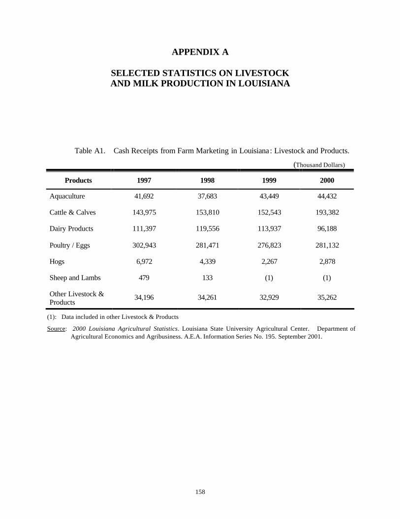
158
APPENDIX A
SELECTED STATISTICS ON LIVESTOCK AND MILK PRODUCTION IN LOUISIANA
Table A1. Cash Receipts from Farm Marketing in Louisiana: Livestock and Products.
(Thousand Dollars)
Products 1997 1998 1999 2000
Aquaculture 41,692 37,683 43,449 44,432
Cattle & Calves 143,975 153,810 152,543 193,382
Dairy Products 111,397 119,556 113,937 96,188
Poultry / Eggs 302,943 281,471 276,823 281,132
Hogs 6,972 4,339 2,267 2,878
Sheep and Lambs 479 133 (1) (1)
Other Livestock & Products
34,196 34,261 32,929 35,262
(1): Data included in other Livestock & Products
Source: 2000 Louisiana Agricultural Statistics. Louisiana State University Agricultural Center. Department of Agricultural Economics and Agribusiness. A.E.A. Information Series No. 195. September 2001.
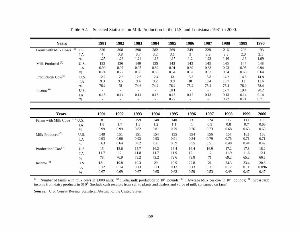
159
Table A2. Selected Statistics on Milk Production in the U.S. and Louisiana : 1981 to 2000.
Years 1981 1982 1983 1984 1985 1986 1987 1988 1989 1990
Farms with Milk Cows (1) U.S. LA
%
320 4
1.25
308 3.8 1.23
298 3.7 1.24
282 3.2 1.13
269 3.1 1.15
249 3
1.2
228 2.8 1.23
216 2.5 1.16
203 2.3 1.13
193 2.1 1.09
Milk Produced (2) U.S. LA %
133 0.99 0.74
136 0.97 0.72
140 0.95 0.68
135 0.89 0.66
143 0.91 0.64
143 0.89 0.62
143 0.88 0.62
145 0.93 0.64
144 0.95 0.66
148 0.94 0.64
Production/ Cow(3) U.S. LA %
12.2 9.3 76.2
12.3 9.6 78
12.6 9.4 74.6
12.4 9.2 74.2
13 9.9 76.2
13.3 10
75.2
13.8 10.4 75.4
14.2 10.7 75.4
14.3 11
76.9
14.8 11.6 78.4
Income (4) U.S. LA %
- 0.15
-
- 0.14
-
- 0.14
-
- 0.13
-
18.1 0.13 0.72
- 0.12
-
- 0.13
-
17.7 0.13 0.72
19.4 0.14 0.71
20.2 0.14 0.71
Years 1991 1992 1993 1994 1995 1996 1997 1998 1999 2000 Farms with Milk Cows (1) U.S.
LA %
181 1.8 0.99
171 1.7 0.99
159 1.3 0.82
148 1.2 0.81
140 1.1 0.79
131 1
0.76
124 0.9 0.73
117 0.8 0.68
111 0.7 0.63
105 0.66 0.63
Milk Produced (2) U.S. LA %
148 0.93 0.63
151 0.96 0.64
151 0.93 0.62
154 0.93 0.6
155 0.91 0.59
154 0.84 0.55
156 0.79 0.51
157 0.75 0.48
163 0.71 0.44
168 0.71 0.42
Production/ Cow(3) U.S. LA %
15 11.7 78
15.6 12
76.9
15.7 11.8 75.2
16.2 11.7 72.2
16.4 11.9 72.6
16.4 12.1 73.8
16.9 12 71
17.2 11.9 69.2
17.8 11.6 65.2
18.2 12.1 66.5
Income (4) U.S. LA %
18.1 0.12 0.67
19.8 0.14 0.69
19.3 0.13 0.67
20 0.13 0.65
19.9 0.12 0.62
22.8 0.13 0.59
21 0.11 0.53
24.3 0.12 0.49
23.4 0.11 0.47
20.8 0.096 0.47
(1) : Number of farms with milk cows in 1,000 units; (2) : Total milk production in 109 pounds; (3) : Average Milk per cow in 103 pounds; (4) : Gross farm income from dairy products in $109 (include cash receipts from sell to plants and dealers and value of milk consumed on farm).
Source: U.S. Census Bureau, Statistical Abstract of the United States.
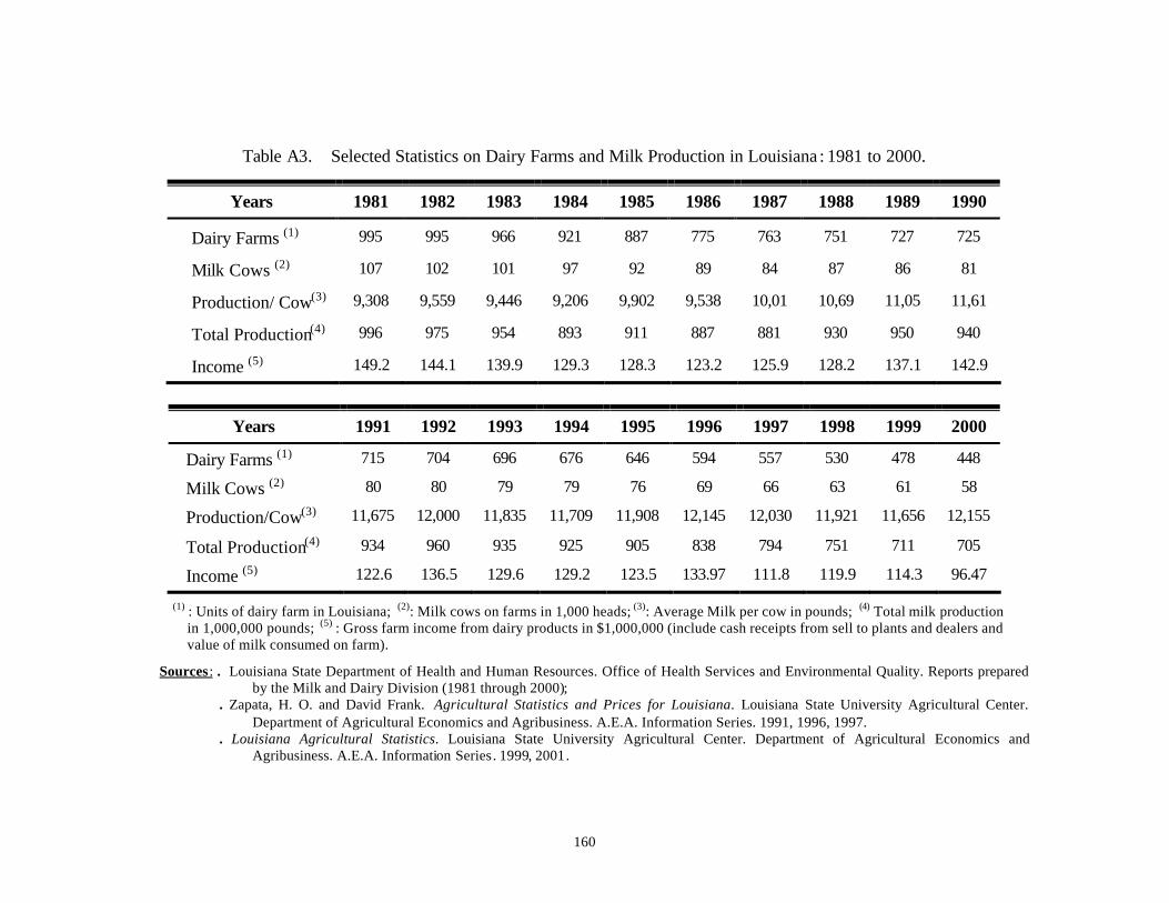
160
Table A3. Selected Statistics on Dairy Farms and Milk Production in Louisiana : 1981 to 2000.
Years 1981 1982 1983 1984 1985 1986 1987 1988 1989 1990
Dairy Farms (1) 995 995 966 921 887 775 763 751 727 725
Milk Cows (2) 107 102 101 97 92 89 84 87 86 81
Production/ Cow(3) 9,308 9,559 9,446 9,206 9,902 9,538 10,01 10,69 11,05 11,61
Total Production(4) 996 975 954 893 911 887 881 930 950 940
Income (5) 149.2 144.1 139.9 129.3 128.3 123.2 125.9 128.2 137.1 142.9
Years 1991 1992 1993 1994 1995 1996 1997 1998 1999 2000
Dairy Farms (1) 715 704 696 676 646 594 557 530 478 448
Milk Cows (2) 80 80 79 79 76 69 66 63 61 58
Production/Cow(3) 11,675 12,000 11,835 11,709 11,908 12,145 12,030 11,921 11,656 12,155
Total Production(4) 934 960 935 925 905 838 794 751 711 705
Income (5) 122.6 136.5 129.6 129.2 123.5 133.97 111.8 119.9 114.3 96.47
(1) : Units of dairy farm in Louisiana; (2): Milk cows on farms in 1,000 heads; (3): Average Milk per cow in pounds; (4) Total milk production in 1,000,000 pounds; (5) : Gross farm income from dairy products in $1,000,000 (include cash receipts from sell to plants and dealers and value of milk consumed on farm).
Sources : . Louisiana State Department of Health and Human Resources. Office of Health Services and Environmental Quality. Reports prepared by the Milk and Dairy Division (1981 through 2000);
. Zapata, H. O. and David Frank. Agricultural Statistics and Prices for Louisiana. Louisiana State University Agricultural Center. Department of Agricultural Economics and Agribusiness. A.E.A. Information Series. 1991, 1996, 1997.
. Louisiana Agricultural Statistics. Louisiana State University Agricultural Center. Department of Agricultural Economics and Agribusiness. A.E.A. Information Series. 1999, 2001.

161
APPENDIX B
THE SURVEY QUESTIONAIRE AND COMPLEMENTARY DOCUMENTS

162
“FIRST LETTER TO PRODUCERS"

163
Department of Agricultural Economics andAgribusiness 101 Agricultural Administration Building Louisiana State University Baton Rouge, LA 70803-5604 (225) 578-3282
FAX: (225) 578-2716 June 26, 2001
Dear Dairy Producer: As you are aware, many Americans have become concerned in recent years with the impact of agriculture on water quality. This has resulted in increased pressure for farmers to adopt management practices that are Aenvironmentally friendly,@ practices that are intended to reduce soil and nutrient runoff into streams. What remains unknown is the extent to which farmers have voluntarily adopted these practices. This survey seeks to determine the extent of adoption of best management practices in the dairy industry, as well as the importance of alternative goals to dairy producers. Your participation in the survey is very important in assuring that as many producers as possible are represented in this study. The reliability of the survey results depends on the participation of producers such as you. All individual responses will be kept strictly confidential. The questionnaire has an identification number for mailing purposes only. This is so that we may check your name off the mailing list when the questionnaire is returned. Your name will never be placed on the questionnaire. We request that the person with primary decision-making authority on the farm complete the survey. Upon receipt of your completed survey, we will send you a check for $10.00. In order for you to receive the payment, you must complete and return the enclosed slip along with the completed survey. The summarized results of the survey will be made available to all interested citizens. Two LSU graduate students in Agricultural Economics will be assisting me in analyzing the data, and will be writing their dissertations based upon the results. Thus, your participation in the study will help them complete their degree requirements. I would be most happy to answer any questions you might have. Please write or call. The telephone number is (225) 578-2759 and my e-mail address is [email protected]. Thank you for your participation.
Sincerely,
Jeffrey M. Gillespie, Ph.D. Associate Professor
THE LOUISIANA AGRICULTURAL EXPERIMENT STATION PROVIDES EQUAL OPPORTUNITIES IN PROGRAMS AND EMPLOYMENT

164
“POSTCARD REMINDER TO PRODUCERS”

165
July 5, 2001
Dear Dairy Producer: Last week, a questionnaire seeking information about your dairy operation was mailed to you. The survey deals with the adoption of best management practices, dairy herd efficiency, and the importance of alternative goals. If you have already completed and returned the survey, please accept our sincere thanks. If not, we would appreciate your returning it as soon as possible. It is important that your response be included in the study if the results are to accurately represent the production characteristics of Louisiana dairy producers. If by some chance you did not receive the questionnaire, or it was misplaced, please call (225) 578-2759. We will send you another one today. Thank you! Sincerely, Jeffrey M. Gillespie, Ph.D.

166
“SECOND REMINDER TO PRODUCERS”

167
Department of Agricultural Economics andAgribusiness 101 Agricultural Administration Building Louisiana State University Baton Rouge, LA 70803-5604
(225) 578-3282 FAX: (225) 578-2716
July 20, 2001 Dear Dairy Producer: About three weeks ago, I wrote to you asking for your participation in a survey on the use of conservation practices and goals of Louisiana dairy producers. As of today, we have not yet received your completed questionnaire. I am writing to you again because of the importance of each survey to the usefulness of this study. The reliability of the study results depends on the participation of producers such as you. The information gathered in this survey will be used to assess the extent of adoption of best management practices in the dairy industry. Results will allow us to determine which practices are being used and the economic forces that affect adoption. We are also assessing the importance of each of seven producer goals with respect to dairy production. Lastly, information collected in this survey will be help us in estimating our annual costs and returns for dairy production. These estimates are useful management tools for dairy producers throughout Louisiana. The survey results will be analyzed by two graduate students in Agricultural Economics. These students' dissertations depend upon a good response rate to this study. All individual responses will be kept strictly confidential . No data on individual responses will ever be reported. The questionnaire has an identification number for mailing purposes only. This is so that we may check your name off the mailing list when the questionnaire is returned. Your name will never be placed on the questionnaire. The questionnaire should be completed by the person with primary decision-making authority on the farm. Because of the importance of this study, we will send you a check for $10.00 upon receipt of the survey. To receive the payment, you must complete and return the enclosed slip along with the completed survey. In the event that your survey has been misplaced, a replacement is enclosed. If you have already responded to the survey and we haven't yet received your response, please accept our sincerest thanks. I would be most happy to answer any questions you might have. Please write or call. The telephone number is (225) 578-2759 and my e-mail address is [email protected].
Your cooperation is greatly appreciated.
Sincerely,
Jeffrey M. Gillespie, Ph.D. Associate Professor
THE LOUISIANA AGRICULTURAL EXPERIMENT STATION PROVIDES EQUAL OPPORTUNITIES IN PROGRAMS AND EMPLOYMENT

168
“SURVEY USED TO COLLECT THE DATA”
169
Use of Conservation Practices and Goals of
Louisiana Dairy Producers
A SURVEY

170
Throughout this survey, you will be asked questions about your dairy operation and how you make production decisions. Please check the answer that best reflects your situation. Note that all information is strictly confidential.
Section I: Production Characteristics 1. How many cows in total do you run in your dairy herd?
________ (number of cows)
2. Do you raise your own replacement heifers? (Circle one)
a) yes b) no 3. What was the average number of pounds of milk produced per cow in your herd in 2000?
________ lbs/cow 4. Which of the following technologies do you use in your operation? (Circle all that apply)
a) Computer b) PC DART program c) Bovine Somatotropin (BSt) d) Artificial Insemination 5. Is your operation a pasture-based operation or a free-stall based operation? (Circle one)
a) Pasture-Based Operation b) Free-Stall Based Operation 6. Please circle any other livestock and/or crops that you raise for sale and/or feeding
(Circle all that apply).
a) Corn e) Oats i) Broilers m) Hay q) Other (Please List) b) Cotton f) Sugarcane j) Sheep n) Vegetable Production _____________ c) Wheat g) Rice k) Goats o) Fruit Production _____________ d) Soybeans h) Hogs l) Beef Cattle p) Forestry _____________
7. How many acres of land are included in your farm operation?
________ (acres) 8. Of the land you farm, how many acres do you own?
________ (acres) 9. How many acres of your farm are devoted to the dairy operation, including the land for crops
supporting the dairy, hay, silage, pasture, barn, feedlot, etc.
________ (acres) 10. Do you raise corn for silage on your dairy operation? (Circle one)
a) yes b) no

171
11. How many family members work on your farm?
_______ (number)
12. How many non-family member employees work on your dairy operation between 1 and 29 hours per
week?
_______ (number)
13. How many non-family member employees work on your dairy operation 30 hours or more per week?
________ (number)
Section II: Goals of Dairy Producers
Dairy producers have a number of goals with respect to their operations. Below are some potential goals that you may have for your operation. Please examine each of the following goals and their definitions and then answer the questions that follow. Maintain and Conserve Land: I want to maintain and conserve the land such that it can be preserved for future generations. Maximize Profit: I want to make the most profit each year given my available resources. Increase Farm Size : I want to increase the size of my operation by controlling more land and/or having newer or larger equipment or buildings. Avoid Years of Loss / Low Profit: I want to avoid years of high losses or low profits. I want to avoid being forced out of business. Increase Net Worth: I want to increase my material and investment accumulations. Have Time for Other Activities: I want to have ample time available for activities other than farming, such as leisure or family activities. Have Family Involved in Agriculture : I want my family to have the opportunity to be involved in agriculture.
Some goals are likely to be more important to you than others. Please rank the following set of goals in the order of your perceived importance. Rank the most important goal as “1”, the least important goal as “7”, and each of the others accordingly. Do not use a ranking more than once. In other words, do not rank two or more goals as equal.
Goal Rank Maintain and Conserve Land: ________ Maximize Profit: ________ Increase Farm Size: ________ Avoid Years of Loss / Low Profit ________ Increase Net Worth: ________ Have Time for Other Activities: ________ Have Family Involved in Agriculture: ________
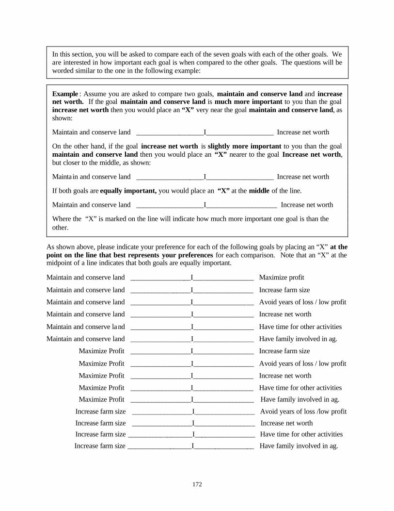
172
In this section, you will be asked to compare each of the seven goals with each of the other goals. We are interested in how important each goal is when compared to the other goals. The questions will be worded similar to the one in the following example:
Example : Assume you are asked to compare two goals, maintain and conserve land and increase net worth. If the goal maintain and conserve land is much more important to you than the goal increase net worth then you would place an “X” very near the goal maintain and conserve land, as shown: Maintain and conserve land ___________________I___________________ Increase net worth On the other hand, if the goal increase net worth is slightly more important to you than the goal maintain and conserve land then you would place an “X” nearer to the goal Increase net worth, but closer to the middle, as shown: Mainta in and conserve land ___________________I___________________ Increase net worth If both goals are equally important, you would place an “X” at the middle of the line. Maintain and conserve land ___________________I____________________ Increase net worth Where the “X” is marked on the line will indicate how much more important one goal is than the other.
As shown above, please indicate your preference for each of the following goals by placing an “X” at the point on the line that best represents your preferences for each comparison. Note that an “X” at the midpoint of a line indicates that both goals are equally important. Maintain and conserve land _________________I_________________ Maximize profit
Maintain and conserve land _________________I_________________ Increase farm size
Maintain and conserve land _________________I_________________ Avoid years of loss / low profit
Maintain and conserve land _________________I_________________ Increase net worth
Maintain and conserve land _________________I_________________ Have time for other activities
Maintain and conserve land _________________I_________________ Have family involved in ag.
Maximize Profit _________________I_________________ Increase farm size
Maximize Profit _________________I_________________ Avoid years of loss / low profit
Maximize Profit _________________I_________________ Increase net worth
Maximize Profit _________________I_________________ Have time for other activities
Maximize Profit _________________I_________________ Have family involved in ag.
Increase farm size _________________I_________________ Avoid years of loss /low profit
Increase farm size _________________I_________________ Increase net worth
Increase farm size __________________I_________________ Have time for other activities
Increase farm size __________________I_________________ Have family involved in ag.

173
Avoid years of loss / low profit _________________I_________________ Increase net worth
Avoid years of loss / low profit _________________I_________________ Have time for other activities
Avoid years of loss / low profit _________________I_________________ Have family involved in ag.
Increase net worth _________________I_________________ Have time for other activities
Increase net worth _________________I_________________ Have family involved in ag.
Have time for other activities _________________I_________________ Have family involved in ag.
Section III: Risk Attitude and Relationship with Community 1. Relative to other investors, how would you characterize yourself? (Circle one)
a) I tend to take on substantial levels of risk in my investment decisions. b) I neither seek nor avoid risk in my investment decisions. c) I tend to avoid risk when possible in my investment decisions.
2. With respect to your farm operation, how important are each of the following relationships with the
other members of your community? (Please circle your response)
NI = not important at all NVI = not very important SI = somewhat important VI = very important
a) Relationship with neighboring farmers NI NVI SI VI
b) Relationship with lending institutions (i.e., banks) NI NVI SI VI
c) Relationship with other agricultural businesses NI NVI SI VI
d) Relationship with neighbors who are non-farmers NI NVI SI VI
e) Relationship with other dairy producers throughout Louisiana NI NVI SI VI
f) Relationship with regulatory agencies NI NVI SI VI
Section IV: Producer and Farm Characteristics 1. Are you male or female? (Circle one)
a) male b) female 2. Are you married? (Circle one)
a) yes b) no 3. Which of the following best describes your ethnic background? (Circle one)
a) American Indian c) Black (African American) e) White (Caucasian)
b) Asian or Pacific Islander d) Hispanic f) Other________________

174
4. What is your age?
________ (years)
5. What is your level of education? (Circle one)
a) Not a High School Graduate c) Technical or College Associate’s Degree e) College Master’s Degree b) High School Graduate d) College Bachelor’s Degree f) College Doctoral Degree
6. How many children 18 years or younger live in your home?
a) None b) 1 c) 2 d) 3 e) 4 f) 5 or more 7. Do any of your children or any other family member plan to take over your dairy operation upon your
retirement?
a) yes b) no c) do not know 8. Please circle the business structure that applies to your dairy farm. (Circle one)
a) Sole Proprietorship b) Partnership c) Family Corporation d) Non-Family Corporation 9. Are you a member of a dairy (milk) cooperative? (Circle one)
a) yes b) no 10. How many years have you been operating your dairy farm? ________ (years)
11. Do you have an off-farm job? (Circle one) a) yes b) no
12. Which of the following best describes your annual household net income? (Circle one)
a) <$20,000 d) $60,000 to $79,999 g) $120,000 to $139,999 b) $20,000 to $39,999 e) $80,000 to $99,999 h) ≥$140,000 c) $40,000 to $59,999 f) $100,000 to $119,999
13. What percentage of your annual household net income comes from your dairy operation? (Circle one)
a) 1 to 20 percent c) 41 to 60 percent e) 81 to 100 percent b) 21 to 40 percent d) 61 to 80 percent
14. What percentage of your annual household net income comes from off-farm employment? (Circle one) a) zero c) 21 to 40 percent e) 61 to 80 percent
b) 1 to 20 percent d) 41 to 60 percent f) 81 to 100 percent 15. Which of the following best describes your current net worth? (Circle one)
a) <$50,000 c) $100,000 to $199,999 e) $400,000 to 799,999 b) $50,000 to $99,999 d) $200,000 to $399,999 f) ≥$800,000

175
16. What is your debt/asset ratio? (Circle one)
a) zero b) 1 to 20 percent c) 21 to 40 percent d) 41 to 60 percent e) over 60 percent
17. On this farm, which generation does the current operator represent (including your family or your spouse’s family)? (Circle one)
a) 1st b) 2nd c) 3rd d) 4th e) 5th f) 6th or more
18. In which parish is your dairy farm located? _____________________________ (the name of parish)
Section V: Best Management Practices 1. Are you aware of the Coastal Non-Point Pollution Control Program (CNPCP) as specified in the
Coastal Zone Management Act? (Circle one)
a) yes b) no 2. Are you aware of efforts to control non-point sources of water pollution through the Clean Water
Act?
a) yes b) no 3. Have you modified the management of your dairy farm as a result of this legislation? (Circle one)
a) yes b) no c) not applicable
4. How would you rate the quality of surface water in your area? (Circle one)
a) very good b) good c) fair d) poor e) very poor
5. What is your primary source of information about water quality problems? (Circle one)
a) Louisiana Cooperative Extension Service b) Government agencies (Natural Resources Conservation Service (NRCS), and others) c) Farm organizations (Farm Bureau, others) d) Other farmers
6. Have you ever heard about BMPs for dairy operations? (Circle one)
a) yes b) no If yes, what is your primary source of information? (Circle one)
a) Louisiana Cooperative Extension Service d) Media (Radio, TV, Magazines, etc.) b) Government agencies (NRCS, others) e) Other ____________________________ c) Farm organizations (Farm Bureau, others)
7. In your opinion, would/does the use of Best Management Practices on your dairy farm improve the
quality of water leaving your land? (Circle one)
a) yes b) no

176
8. Please check any of the practices that you currently implement under “yes” column. In cases where you have not implemented a BMP, please indicate your reason for non-implementation under the appropriate “no” column. Please check only one box in each row. A description of the management practices is provided following on the next page.
Current Adoption
No
Management Practices
Yes Need More Information
High Cost of Implementation
Have Not Heard of It
Not Applicable to my Farm
Conservation Tillage Practices
Cover and Green Manure Crop
Critical Area Planting
Fence
Field Borders
Filter Strips
Grassed Waterway
Heavy Use Area Protection
Nutrient Management
Pest Management
Prescribed Grazing
Regulating Water in Drainage System
Riparian Forest Buffer
Roof Runoff Management
Sediment Basin
Streambank and Shoreline Protection
Trough or Tank
Waste Management System
Waste Storage Facility
Waste Treatment Lagoon
Waste Utilization

177
Description
Conservation Tillage Practices: A system designed to manage the amount, orientation and distribution of crop and other plant residues on the soil surface year-round.
Cover and Green Manure Crop: A crop of close growing grasses, legumes or small grains grown primarily for seasonal protection and soil improvement.
Critical Area Planting: A planting of vegetation such as trees, shrubs, vines, grasses or legumes on highly erodible areas.
Fence: A constructed barrier to livestock, wildlife or people to facilitate the application of conservation practices.
Field Borders: Strips of perennial vegetation to control erosion and protect the edges of a field.
Filter Strips: Areas of vegetation planted around fields to remove wastewater sediment and nutrients from runoff.
Grassed Waterway: A channel that is shaped or graded to required dimensions and established in suitable vegetation to convey runoff from terraces, diversion or other water concentration.
Heavy Use Area Protection: Protection of heavily used areas by establishing vegetative cover.
Nutrient Management: Management of the amount, form, placement and timing of application of plant nutrients (fertilizers) for optimum forage and crop yields.
Pest Management: A pest management program consistent with crop production goals and environmental standards.
Prescribed Grazing: Controlled harvest of vegetation with grazing animals.
Regulating Water in Drainage System: To control the removal of surface runoff, primarily through the operation of water control structures.
Riparian Forest Buffer: An area of trees, shrubs and other vegetation located adjacent to watercourses or water bodies.
Roof Runoff Management: A facility for collecting, controlling and disposing of roof runoff water.
Sediment Basin: A basin to collect and store debris or sediment.
Streambank and Shoreline Protection: Use of vegetation or structures to stabilize and protect banks of streams and lakes against scour and erosion.
Trough or Tank: A trough or tank with needed devices for water control and waste disposal installed to provide drinking water for livestock.
Waste Management System: A planned system for managing liquid and solid waste including runoff from concentrated waste areas.
Waste Storage Facility: An impoundment to temporarily store manure, wastewater and contaminated runoff.
Waste Treatment Lagoon: An impoundment to biologically treat organic waste, reduce pollution and protect the environment.
Waste Utilization: Use of agricultural waste on land in an environmentally acceptable manner to provide fertility for crop forage, and to improve or maintain soil structure.

178
9. Have you developed and/or updated a dairy farm plan with NRCS within the last three years?
a) yes b) no 10. Of the land on your dairy farm, approximately what percentage would be classified as “highly
erodible”? (Circle one)
a) 0 to 19 percent c) 40 to 59 percent e) 80 to 100 percent b) 20 to 39 percent d) 60 to 70 percent
11. Of the land on your dairy farm, approximately what percentage would you classify as “well-drained”? (Circle one)
a) 0 to 19 percent c) 40 to 59 percent e) 80 to 100 percent b) 20 to 39 percent d) 60 to 70 percent
12. How far from your dairy farm is the nearest neighboring dairy farm? (Circle one)
a) < 1 mile b) 1 to 5 miles c) > 5 miles
13. How far from your dairy farm is the nearest stream or river? (Circle one)
a) a stream / river runs through my farm c) between one-half mile and one mile b) less than half a mile d) more than one mile
14. During the last year, how often did you meet with Louisiana Cooperative Extension Service personnel?
________ (number of times)
15. During the last year, how often did you meet with NRCS personnel?
________ (number of times)
16. Are you a member of the Dairy Herd Improvement Association (DHIA)? (Circle one)
a) yes b) no
17. Have you participated in any dairy cost-sharing programs while implementing a BMP? (Circle one)
a) yes b) no 18. How many seminars and/or meetings did you attend in 2000 that dealt with dairy production and/or dairy industry issues?
________ (number)
19. How many farm magazines did you subscribe to in 2000? (i.e., an annual subscription to Farm Journal would be considered one subscription.) ________ (number) 20. How many dairy-related university publications did you read in 2000? ________ (number)
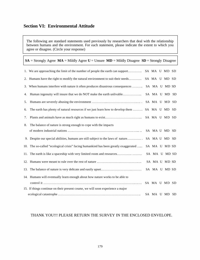
179
Section VI: Environmental Attitude
The following are standard statements used previously by researchers that deal with the relationship between humans and the environment. For each statement, please indicate the extent to which you agree or disagree. (Circle your response)
SA = Strongly Agree MA = Mildly Agree U = Unsure MD = Mildly Disagree SD = Strongly Disagree
1. We are approaching the limit of the number of people the earth can support…………. SA MA U MD SD
2. Humans have the right to modify the natural environment to suit their needs………… SA MA U MD SD
3. When humans interfere with nature it often produces disastrous consequences ………. SA MA U MD SD
4. Human ingenuity will insure that we do NOT make the earth unlivable……………... SA MA U MD SD
5. Humans are severely abusing the environment …………...…………………………. . SA MA U MD SD
6. The earth has plenty of natural resources if we just learn how to develop them ……… SA MA U MD SD
7. Plants and animals have as much right as humans to exist.………………………….... SA MA U MD SD
8. The balance of nature is strong enough to cope with the impacts
of modern industrial nations .…..……………………….……………………….…... .. SA MA U MD SD
9. Despite our special abilities, humans are still subject to the laws of nature…………. . SA MA U MD SD
10. The so-called “ecological crisis” facing humankind has been greatly exaggerated …... SA MA U MD SD
11. The earth is like a spaceship with very limited room and resources………….. ……… SA MA U MD SD
12. Humans were meant to rule over the rest of nature ..…………………………………. SA MA U MD SD
13. The balance of nature is very delicate and easily upset………………………..……… SA MA U MD SD
14. Humans will eventually learn enough about how nature works to be able to
control it …………………………………………………………………………….… SA MA U MD SD
15. If things continue on their present course, we will soon experience a major
ecological catastrophe .…………………………………….…………………………... SA MA U MD SD
THANK YOU!!! PLEASE RETURN THE SURVEY IN THE ENCLOSED ENVELOPE.

180
APPENDIX C
COLLINEARITY DIAGNOSTICS RESULTS
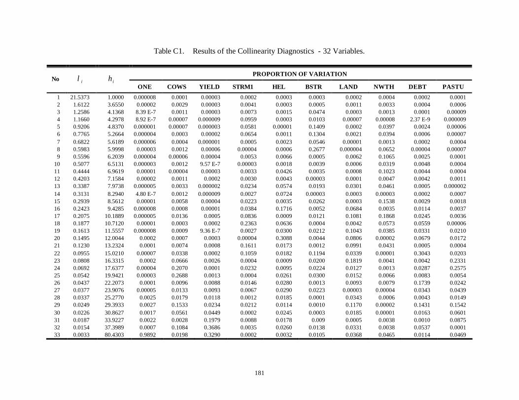
181
Table C1. Results of the Collinearity Diagnostics - 32 Variables.
PROPORTION OF VARIATION No iλ iη
ONE COWS YIELD STRM1 HEL BSTR LAND NWTH DEBT PASTU
1 21.5373 1.0000 0.000008 0.0001 0.00003 0.0002 0.0003 0.0003 0.0002 0.0004 0.0002 0.0001 2 1.6122 3.6550 0.00002 0.0029 0.00003 0.0041 0.0003 0.0005 0.0011 0.0033 0.0004 0.0006 3 1.2586 4.1368 8.39 E-7 0.0011 0.00003 0.0073 0.0015 0.0474 0.0003 0.0013 0.0001 0.00009 4 1.1660 4.2978 8.92 E-7 0.00007 0.000009 0.0959 0.0003 0.0103 0.00007 0.00008 2.37 E-9 0.000009 5 0.9206 4.8370 0.000001 0.00007 0.000003 0.0581 0.00001 0.1409 0.0002 0.0397 0.0024 0.00006 6 0.7765 5.2664 0.000004 0.0003 0.00002 0.0654 0.0011 0.1304 0.0021 0.0394 0.0006 0.00007 7 0.6822 5.6189 0.000006 0.0004 0.000001 0.0005 0.0023 0.0546 0.00001 0.0013 0.0002 0.0004 8 0.5983 5.9998 0.00003 0.0012 0.00006 0.00004 0.0006 0.2677 0.000004 0.0652 0.00004 0.00007 9 0.5596 6.2039 0.000004 0.00006 0.00004 0.0053 0.0066 0.0005 0.0062 0.1065 0.0025 0.0001
10 0.5077 6.5131 0.000003 0.0012 9.57 E-7 0.00003 0.0018 0.0039 0.0006 0.0319 0.0048 0.0004 11 0.4444 6.9619 0.00001 0.00004 0.00003 0.0033 0.0426 0.0035 0.0008 0.1023 0.0044 0.0004 12 0.4203 7.1584 0.00002 0.0011 0.0002 0.0030 0.0043 0.00003 0.0001 0.0047 0.0042 0.0011 13 0.3387 7.9738 0.000005 0.0033 0.000002 0.0234 0.0574 0.0193 0.0301 0.0461 0.0005 0.000002 14 0.3131 8.2940 4.80 E-7 0.0012 0.000009 0.0027 0.0724 0.00003 0.0003 0.00003 0.0002 0.0007 15 0.2939 8.5612 0.00001 0.0058 0.00004 0.0223 0.0035 0.0262 0.0003 0.1538 0.0029 0.0018 16 0.2423 9.4285 0.000008 0.0008 0.00001 0.0384 0.1716 0.0052 0.0684 0.0035 0.0114 0.0037 17 0.2075 10.1889 0.000005 0.0136 0.0005 0.0836 0.0009 0.0121 0.1081 0.1868 0.0245 0.0036 18 0.1877 10.7120 0.00001 0.0003 0.0002 0.2363 0.0636 0.0004 0.0042 0.0573 0.0559 0.00006 19 0.1613 11.5557 0.000008 0.0009 9.36 E-7 0.0027 0.0300 0.0212 0.1043 0.0385 0.0331 0.0210 20 0.1495 12.0044 0.0002 0.0007 0.0003 0.00004 0.3088 0.0044 0.0806 0.00002 0.0679 0.0172 21 0.1230 13.2324 0.0001 0.0074 0.0008 0.1611 0.0173 0.0012 0.0991 0.0431 0.0005 0.0004 22 0.0955 15.0210 0.00007 0.0338 0.0002 0.1059 0.0182 0.1194 0.0339 0.00001 0.3043 0.0203 23 0.0808 16.3315 0.0002 0.0666 0.0026 0.0004 0.0009 0.0200 0.1819 0.0041 0.0042 0.2331 24 0.0692 17.6377 0.00004 0.2070 0.0001 0.0232 0.0095 0.0224 0.0127 0.0013 0.0287 0.2575 25 0.0542 19.9421 0.00003 0.2688 0.0013 0.0004 0.0261 0.0300 0.0152 0.0066 0.0083 0.0054 26 0.0437 22.2073 0.0001 0.0096 0.0088 0.0146 0.0280 0.0013 0.0093 0.0079 0.1739 0.0242 27 0.0377 23.9076 0.00005 0.0133 0.0093 0.0067 0.0290 0.0223 0.00003 0.00004 0.0343 0.0439 28 0.0337 25.2770 0.0025 0.0179 0.0118 0.0012 0.0185 0.0001 0.0343 0.0006 0.0043 0.0149 29 0.0249 29.3933 0.0027 0.1533 0.0234 0.0212 0.0114 0.0010 0.1170 0.00002 0.1431 0.1542 30 0.0226 30.8627 0.0017 0.0561 0.0449 0.0002 0.0245 0.0003 0.0185 0.00001 0.0163 0.0601 31 0.0187 33.9227 0.0022 0.0028 0.1979 0.0088 0.0178 0.009 0.0005 0.0038 0.0010 0.0875 32 0.0154 37.3989 0.0007 0.1084 0.3686 0.0035 0.0260 0.0138 0.0331 0.0038 0.0537 0.0001 33 0.0033 80.4303 0.9892 0.0198 0.3290 0.0002 0.0032 0.0105 0.0368 0.0465 0.0114 0.0469
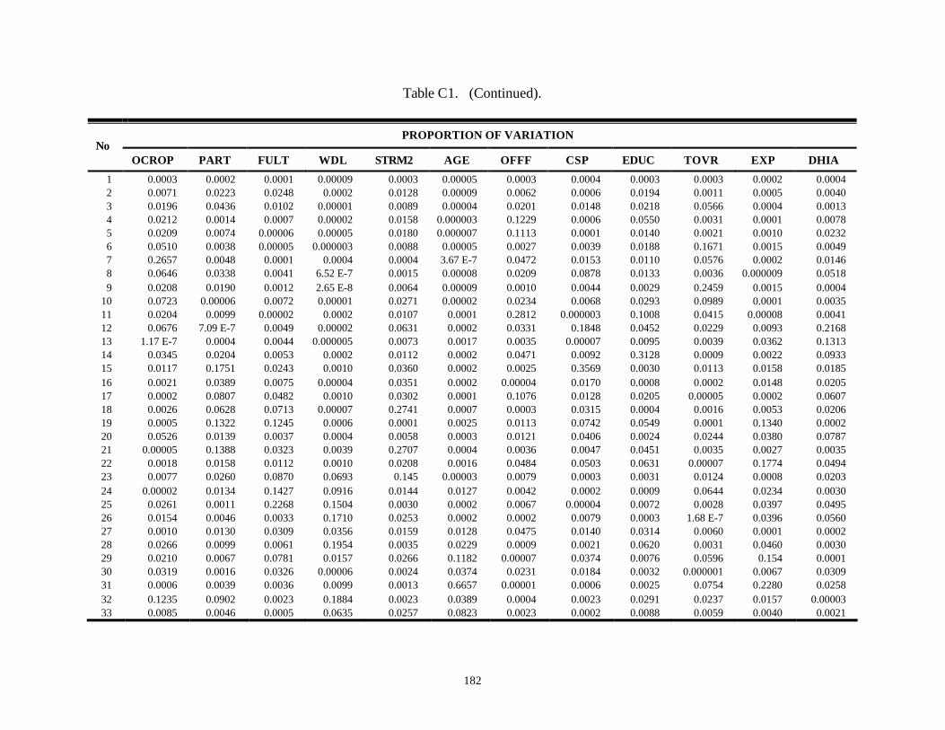
182
Table C1. (Continued).
PROPORTION OF VARIATION No
OCROP PART FULT WDL STRM2 AGE OFFF CSP EDUC TOVR EXP DHIA
1 0.0003 0.0002 0.0001 0.00009 0.0003 0.00005 0.0003 0.0004 0.0003 0.0003 0.0002 0.0004 2 0.0071 0.0223 0.0248 0.0002 0.0128 0.00009 0.0062 0.0006 0.0194 0.0011 0.0005 0.0040 3 0.0196 0.0436 0.0102 0.00001 0.0089 0.00004 0.0201 0.0148 0.0218 0.0566 0.0004 0.0013 4 0.0212 0.0014 0.0007 0.00002 0.0158 0.000003 0.1229 0.0006 0.0550 0.0031 0.0001 0.0078 5 0.0209 0.0074 0.00006 0.00005 0.0180 0.000007 0.1113 0.0001 0.0140 0.0021 0.0010 0.0232 6 0.0510 0.0038 0.00005 0.000003 0.0088 0.00005 0.0027 0.0039 0.0188 0.1671 0.0015 0.0049 7 0.2657 0.0048 0.0001 0.0004 0.0004 3.67 E-7 0.0472 0.0153 0.0110 0.0576 0.0002 0.0146 8 0.0646 0.0338 0.0041 6.52 E-7 0.0015 0.00008 0.0209 0.0878 0.0133 0.0036 0.000009 0.0518 9 0.0208 0.0190 0.0012 2.65 E-8 0.0064 0.00009 0.0010 0.0044 0.0029 0.2459 0.0015 0.0004
10 0.0723 0.00006 0.0072 0.00001 0.0271 0.00002 0.0234 0.0068 0.0293 0.0989 0.0001 0.0035 11 0.0204 0.0099 0.00002 0.0002 0.0107 0.0001 0.2812 0.000003 0.1008 0.0415 0.00008 0.0041 12 0.0676 7.09 E-7 0.0049 0.00002 0.0631 0.0002 0.0331 0.1848 0.0452 0.0229 0.0093 0.2168 13 1.17 E-7 0.0004 0.0044 0.000005 0.0073 0.0017 0.0035 0.00007 0.0095 0.0039 0.0362 0.1313 14 0.0345 0.0204 0.0053 0.0002 0.0112 0.0002 0.0471 0.0092 0.3128 0.0009 0.0022 0.0933 15 0.0117 0.1751 0.0243 0.0010 0.0360 0.0002 0.0025 0.3569 0.0030 0.0113 0.0158 0.0185 16 0.0021 0.0389 0.0075 0.00004 0.0351 0.0002 0.00004 0.0170 0.0008 0.0002 0.0148 0.0205 17 0.0002 0.0807 0.0482 0.0010 0.0302 0.0001 0.1076 0.0128 0.0205 0.00005 0.0002 0.0607 18 0.0026 0.0628 0.0713 0.00007 0.2741 0.0007 0.0003 0.0315 0.0004 0.0016 0.0053 0.0206 19 0.0005 0.1322 0.1245 0.0006 0.0001 0.0025 0.0113 0.0742 0.0549 0.0001 0.1340 0.0002 20 0.0526 0.0139 0.0037 0.0004 0.0058 0.0003 0.0121 0.0406 0.0024 0.0244 0.0380 0.0787 21 0.00005 0.1388 0.0323 0.0039 0.2707 0.0004 0.0036 0.0047 0.0451 0.0035 0.0027 0.0035 22 0.0018 0.0158 0.0112 0.0010 0.0208 0.0016 0.0484 0.0503 0.0631 0.00007 0.1774 0.0494 23 0.0077 0.0260 0.0870 0.0693 0.145 0.00003 0.0079 0.0003 0.0031 0.0124 0.0008 0.0203 24 0.00002 0.0134 0.1427 0.0916 0.0144 0.0127 0.0042 0.0002 0.0009 0.0644 0.0234 0.0030 25 0.0261 0.0011 0.2268 0.1504 0.0030 0.0002 0.0067 0.00004 0.0072 0.0028 0.0397 0.0495 26 0.0154 0.0046 0.0033 0.1710 0.0253 0.0002 0.0002 0.0079 0.0003 1.68 E-7 0.0396 0.0560 27 0.0010 0.0130 0.0309 0.0356 0.0159 0.0128 0.0475 0.0140 0.0314 0.0060 0.0001 0.0002 28 0.0266 0.0099 0.0061 0.1954 0.0035 0.0229 0.0009 0.0021 0.0620 0.0031 0.0460 0.0030 29 0.0210 0.0067 0.0781 0.0157 0.0266 0.1182 0.00007 0.0374 0.0076 0.0596 0.154 0.0001 30 0.0319 0.0016 0.0326 0.00006 0.0024 0.0374 0.0231 0.0184 0.0032 0.000001 0.0067 0.0309 31 0.0006 0.0039 0.0036 0.0099 0.0013 0.6657 0.00001 0.0006 0.0025 0.0754 0.2280 0.0258 32 0.1235 0.0902 0.0023 0.1884 0.0023 0.0389 0.0004 0.0023 0.0291 0.0237 0.0157 0.00003 33 0.0085 0.0046 0.0005 0.0635 0.0257 0.0823 0.0023 0.0002 0.0088 0.0059 0.0040 0.0021
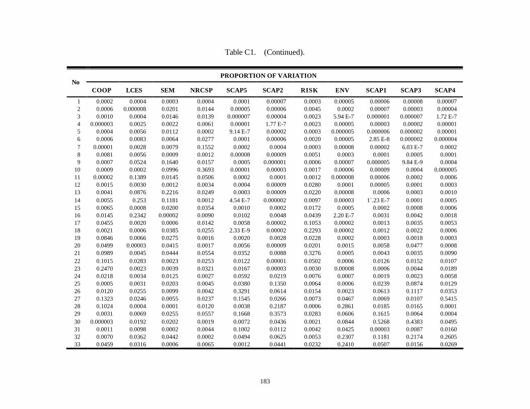
183
Table C1. (Continued).
PROPORTION OF VARIATION No
COOP LCES SEM NRCSP SCAP5 SCAP2 RISK ENV SCAP1 SCAP3 SCAP4
1 0.0002 0.0004 0.0003 0.0004 0.0001 0.00007 0.0003 0.00005 0.00006 0.00008 0.00007 2 0.0006 0.000008 0.0201 0.0144 0.00005 0.00006 0.0045 0.0002 0.00007 0.00003 0.00004 3 0.0010 0.0004 0.0146 0.0139 0.000007 0.00004 0.0023 5.94 E-7 0.000001 0.000007 1.72 E-7 4 0.000003 0.0025 0.0022 0.0061 0.00001 1.77 E-7 0.0023 0.00005 0.00003 0.00002 0.00001 5 0.0004 0.0056 0.0112 0.0002 9.14 E-7 0.00002 0.0003 0.000005 0.000006 0.000002 0.00001 6 0.0006 0.0083 0.0064 0.0277 0.0001 0.00006 0.0020 0.00005 2.85 E-8 0.000002 0.000004 7 0.00001 0.0028 0.0079 0.1552 0.0002 0.0004 0.0003 0.00008 0.00002 6.03 E-7 0.0002 8 0.0081 0.0056 0.0009 0.0012 0.00008 0.00009 0.0051 0.0003 0.0001 0.0005 0.0001 9 0.0007 0.0524 0.1640 0.0157 0.0005 0.000001 0.0006 0.00007 0.000005 9.84 E-9 0.0004
10 0.0009 0.0002 0.0996 0.3693 0.00001 0.00003 0.0017 0.00006 0.00009 0.0004 0.000005 11 0.00002 0.1389 0.0145 0.0506 0.0002 0.0001 0.0012 0.000008 0.00006 0.0002 0.0006 12 0.0015 0.0030 0.0012 0.0034 0.0004 0.00009 0.0280 0.0001 0.00005 0.0001 0.0003 13 0.0041 0.0876 0.2216 0.0249 0.0003 0.00009 0.0220 0.00008 0.0006 0.0003 0.0010 14 0.0055 0.253 0.1181 0.0012 4.54 E-7 0.000002 0.0097 0.00003 1`.23 E-7 0.0001 0.0005 15 0.0065 0.0008 0.0200 0.0354 0.0010 0.0002 0.0172 0.0005 0.0002 0.0008 0.0006 16 0.0145 0.2342 0.00002 0.0090 0.0102 0.0048 0.0439 2.20 E-7 0.0031 0.0042 0.0018 17 0.0455 0.0020 0.0006 0.0142 0.0058 0.00002 0.1053 0.00002 0.0013 0.0035 0.0053 18 0.0021 0.0006 0.0385 0.0255 2.33 E-9 0.00002 0.2293 0.00002 0.0012 0.0022 0.0006 19 0.0846 0.0066 0.0275 0.0016 0.0020 0.0028 0.0228 0.0002 0.0003 0.0018 0.0003 20 0.0499 0.00003 0.0415 0.0017 0.0056 0.00009 0.0201 0.0015 0.0058 0.0477 0.0008 21 0.0989 0.0045 0.0444 0.0554 0.0352 0.0088 0.3276 0.0005 0.0043 0.0035 0.0090 22 0.1015 0.0283 0.0023 0.0253 0.0122 0.00001 0.0502 0.0006 0.0126 0.0152 0.0107 23 0.2470 0.0023 0.0039 0.0321 0.0167 0.00003 0.0030 0.00008 0.0006 0.0044 0.0189 24 0.0218 0.0034 0.0125 0.0027 0.0592 0.0219 0.0076 0.0007 0.0019 0.0023 0.0058 25 0.0005 0.0031 0.0203 0.0045 0.0380 0.1350 0.0064 0.0006 0.0239 0.0874 0.0129 26 0.0120 0.0255 0.0099 0.0042 0.3291 0.0614 0.0154 0.0023 0.0613 0.1117 0.0353 27 0.1323 0.0246 0.0055 0.0237 0.1545 0.0266 0.0073 0.0467 0.0069 0.0107 0.5415 28 0.1024 0.0004 0.0001 0.0120 0.0038 0.2187 0.0006 0.2861 0.0185 0.0165 0.0001 29 0.0031 0.0069 0.0255 0.0557 0.1668 0.3573 0.0283 0.0606 0.1615 0.0064 0.0004 30 0.000003 0.0192 0.0202 0.0019 0.0072 0.0436 0.0021 0.0844 0.5268 0.4383 0.0495 31 0.0011 0.0098 0.0002 0.0044 0.1002 0.0112 0.0042 0.0425 0.00003 0.0087 0.0160 32 0.0070 0.0362 0.0442 0.0002 0.0494 0.0625 0.0053 0.2307 0.1181 0.2174 0.2605 33 0.0459 0.0316 0.0006 0.0065 0.0012 0.0441 0.0232 0.2410 0.0507 0.0156 0.0269
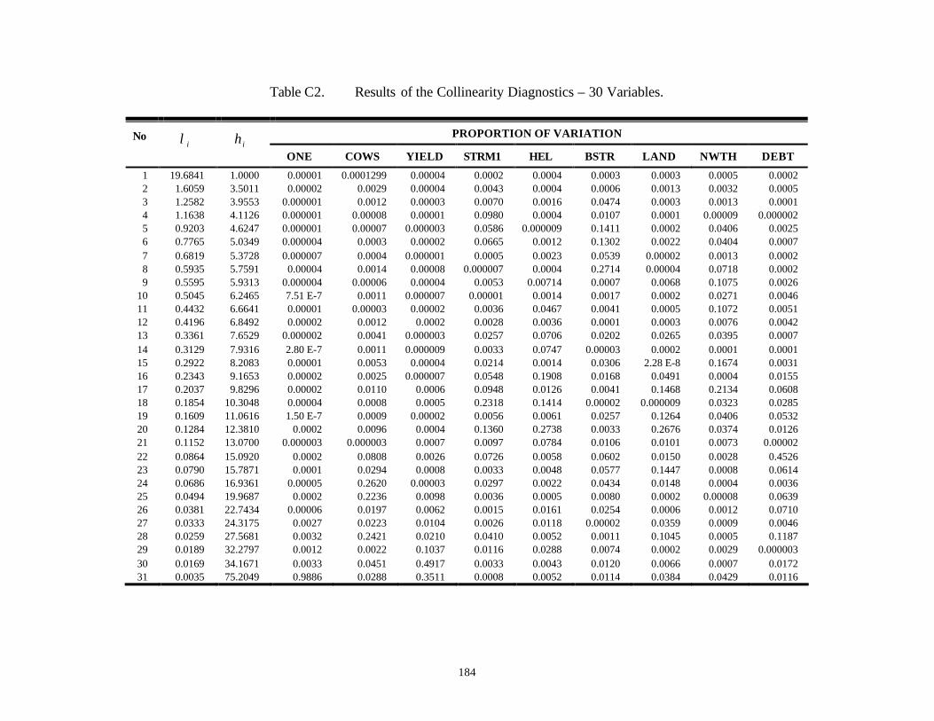
184
Table C2. Results of the Collinearity Diagnostics – 30 Variables.
PROPORTION OF VARIATION No iλ iη
ONE COWS YIELD STRM1 HEL BSTR LAND NWTH DEBT
1 19.6841 1.0000 0.00001 0.0001299 0.00004 0.0002 0.0004 0.0003 0.0003 0.0005 0.0002 2 1.6059 3.5011 0.00002 0.0029 0.00004 0.0043 0.0004 0.0006 0.0013 0.0032 0.0005 3 1.2582 3.9553 0.000001 0.0012 0.00003 0.0070 0.0016 0.0474 0.0003 0.0013 0.0001 4 1.1638 4.1126 0.000001 0.00008 0.00001 0.0980 0.0004 0.0107 0.0001 0.00009 0.000002 5 0.9203 4.6247 0.000001 0.00007 0.000003 0.0586 0.000009 0.1411 0.0002 0.0406 0.0025 6 0.7765 5.0349 0.000004 0.0003 0.00002 0.0665 0.0012 0.1302 0.0022 0.0404 0.0007 7 0.6819 5.3728 0.000007 0.0004 0.000001 0.0005 0.0023 0.0539 0.00002 0.0013 0.0002 8 0.5935 5.7591 0.00004 0.0014 0.00008 0.000007 0.0004 0.2714 0.00004 0.0718 0.0002 9 0.5595 5.9313 0.000004 0.00006 0.00004 0.0053 0.00714 0.0007 0.0068 0.1075 0.0026
10 0.5045 6.2465 7.51 E-7 0.0011 0.000007 0.00001 0.0014 0.0017 0.0002 0.0271 0.0046 11 0.4432 6.6641 0.00001 0.00003 0.00002 0.0036 0.0467 0.0041 0.0005 0.1072 0.0051 12 0.4196 6.8492 0.00002 0.0012 0.0002 0.0028 0.0036 0.0001 0.0003 0.0076 0.0042 13 0.3361 7.6529 0.000002 0.0041 0.000003 0.0257 0.0706 0.0202 0.0265 0.0395 0.0007 14 0.3129 7.9316 2.80 E-7 0.0011 0.000009 0.0033 0.0747 0.00003 0.0002 0.0001 0.0001 15 0.2922 8.2083 0.00001 0.0053 0.00004 0.0214 0.0014 0.0306 2.28 E-8 0.1674 0.0031 16 0.2343 9.1653 0.00002 0.0025 0.000007 0.0548 0.1908 0.0168 0.0491 0.0004 0.0155 17 0.2037 9.8296 0.00002 0.0110 0.0006 0.0948 0.0126 0.0041 0.1468 0.2134 0.0608 18 0.1854 10.3048 0.00004 0.0008 0.0005 0.2318 0.1414 0.00002 0.000009 0.0323 0.0285 19 0.1609 11.0616 1.50 E-7 0.0009 0.00002 0.0056 0.0061 0.0257 0.1264 0.0406 0.0532 20 0.1284 12.3810 0.0002 0.0096 0.0004 0.1360 0.2738 0.0033 0.2676 0.0374 0.0126 21 0.1152 13.0700 0.000003 0.000003 0.0007 0.0097 0.0784 0.0106 0.0101 0.0073 0.00002 22 0.0864 15.0920 0.0002 0.0808 0.0026 0.0726 0.0058 0.0602 0.0150 0.0028 0.4526 23 0.0790 15.7871 0.0001 0.0294 0.0008 0.0033 0.0048 0.0577 0.1447 0.0008 0.0614 24 0.0686 16.9361 0.00005 0.2620 0.00003 0.0297 0.0022 0.0434 0.0148 0.0004 0.0036 25 0.0494 19.9687 0.0002 0.2236 0.0098 0.0036 0.0005 0.0080 0.0002 0.00008 0.0639 26 0.0381 22.7434 0.00006 0.0197 0.0062 0.0015 0.0161 0.0254 0.0006 0.0012 0.0710 27 0.0333 24.3175 0.0027 0.0223 0.0104 0.0026 0.0118 0.00002 0.0359 0.0009 0.0046 28 0.0259 27.5681 0.0032 0.2421 0.0210 0.0410 0.0052 0.0011 0.1045 0.0005 0.1187 29 0.0189 32.2797 0.0012 0.0022 0.1037 0.0116 0.0288 0.0074 0.0002 0.0029 0.000003 30 0.0169 34.1671 0.0033 0.0451 0.4917 0.0033 0.0043 0.0120 0.0066 0.0007 0.0172 31 0.0035 75.2049 0.9886 0.0288 0.3511 0.0008 0.0052 0.0114 0.0384 0.0429 0.0116
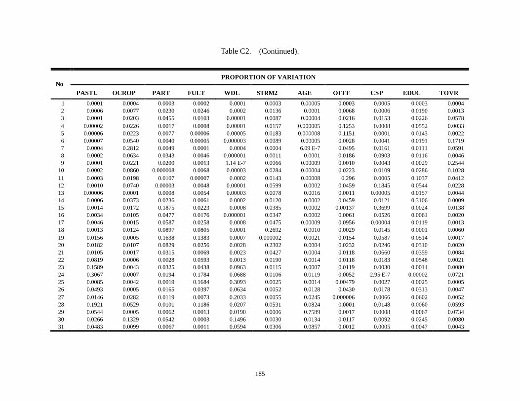
185
Table C2. (Continued).
PROPORTION OF VARIATION No
PASTU OCROP PART FULT WDL STRM2 AGE OFFF CSP EDUC TOVR
1 0.0001 0.0004 0.0003 0.0002 0.0001 0.0003 0.00005 0.0003 0.0005 0.0003 0.0004 2 0.0006 0.0077 0.0230 0.0246 0.0002 0.0136 0.0001 0.0068 0.0006 0.0190 0.0013 3 0.0001 0.0203 0.0455 0.0103 0.00001 0.0087 0.00004 0.0216 0.0153 0.0226 0.0578 4 0.00002 0.0226 0.0017 0.0008 0.00001 0.0157 0.000005 0.1253 0.0008 0.0552 0.0033 5 0.00006 0.0223 0.0077 0.00006 0.00005 0.0183 0.000008 0.1151 0.0001 0.0143 0.0022 6 0.00007 0.0540 0.0040 0.00005 0.000003 0.0089 0.00005 0.0028 0.0041 0.0191 0.1719 7 0.0004 0.2812 0.0049 0.0001 0.0004 0.0004 6.09 E-7 0.0495 0.0161 0.0111 0.0591 8 0.0002 0.0634 0.0343 0.0046 0.000001 0.0011 0.0001 0.0186 0.0903 0.0116 0.0046 9 0.0001 0.0221 0.0200 0.0013 1.14 E-7 0.0066 0.00009 0.0010 0.0043 0.0029 0.2544
10 0.0002 0.0860 0.000008 0.0068 0.00003 0.0284 0.00004 0.0223 0.0109 0.0286 0.1028 11 0.0003 0.0198 0.0107 0.00007 0.0002 0.0143 0.00008 0.296 0.0005 0.1037 0.0412 12 0.0010 0.0740 0.00003 0.0048 0.00001 0.0599 0.0002 0.0459 0.1845 0.0544 0.0228 13 0.00006 0.0001 0.0008 0.0054 0.00003 0.0078 0.0016 0.0011 0.00005 0.0157 0.0044 14 0.0006 0.0373 0.0236 0.0061 0.0002 0.0120 0.0002 0.0459 0.0121 0.3106 0.0009 15 0.0014 0.0172 0.1875 0.0223 0.0008 0.0385 0.0002 0.00137 0.3699 0.0024 0.0138 16 0.0034 0.0105 0.0477 0.0176 0.000001 0.0347 0.0002 0.0061 0.0526 0.0061 0.0020 17 0.0046 0.0015 0.0587 0.0258 0.0008 0.0475 0.00009 0.0956 0.00004 0.0119 0.0013 18 0.0013 0.0124 0.0897 0.0805 0.0001 0.2692 0.0010 0.0029 0.0145 0.0001 0.0060 19 0.0156 0.0005 0.1638 0.1383 0.0007 0.000002 0.0021 0.0154 0.0587 0.0514 0.0017 20 0.0182 0.0107 0.0829 0.0256 0.0028 0.2302 0.0004 0.0232 0.0246 0.0310 0.0020 21 0.0105 0.0017 0.0315 0.0069 0.0023 0.0427 0.0004 0.0118 0.0660 0.0359 0.0084 22 0.0819 0.0006 0.0028 0.0593 0.0013 0.0190 0.0014 0.0118 0.0183 0.0548 0.0021 23 0.1589 0.0043 0.0325 0.0438 0.0963 0.0115 0.0007 0.0119 0.0030 0.0014 0.0080 24 0.3067 0.0007 0.0194 0.1784 0.0688 0.0106 0.0119 0.0052 2.95 E-7 0.00002 0.0721 25 0.0085 0.0042 0.0019 0.1684 0.3093 0.0025 0.0014 0.00479 0.0027 0.0025 0.0005 26 0.0493 0.0005 0.0165 0.0397 0.0634 0.0052 0.0128 0.0430 0.0178 0.0313 0.0047 27 0.0146 0.0282 0.0119 0.0073 0.2033 0.0055 0.0245 0.000006 0.0066 0.0602 0.0052 28 0.1921 0.0529 0.0101 0.1186 0.0207 0.0531 0.0824 0.0001 0.0148 0.0060 0.0593 29 0.0544 0.0005 0.0062 0.0013 0.0190 0.0006 0.7589 0.0017 0.0008 0.0067 0.0734 30 0.0266 0.1329 0.0542 0.0003 0.1496 0.0030 0.0134 0.0117 0.0092 0.0245 0.0080 31 0.0483 0.0099 0.0067 0.0011 0.0594 0.0306 0.0857 0.0012 0.0005 0.0047 0.0043
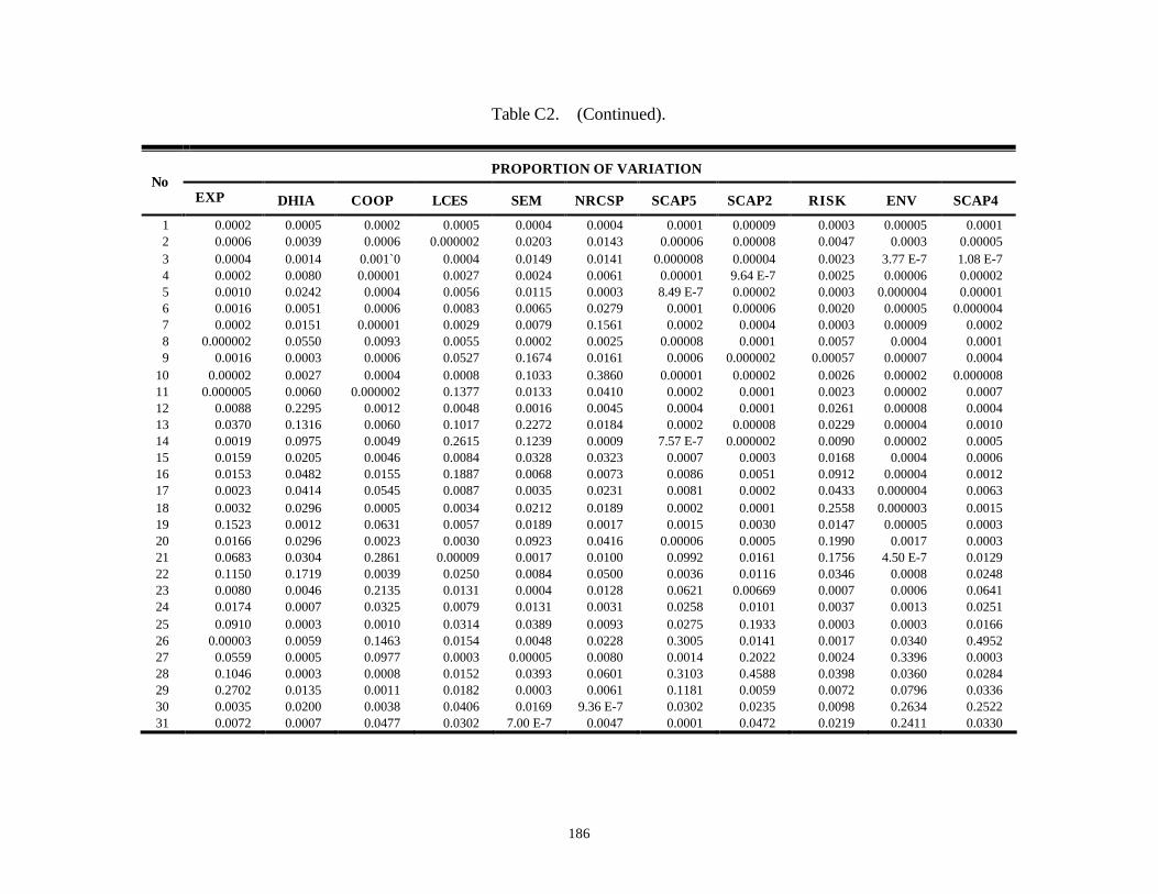
186
Table C2. (Continued).
PROPORTION OF VARIATION No
EXP DHIA COOP LCES SEM NRCSP SCAP5 SCAP2 RISK ENV SCAP4
1 0.0002 0.0005 0.0002 0.0005 0.0004 0.0004 0.0001 0.00009 0.0003 0.00005 0.0001 2 0.0006 0.0039 0.0006 0.000002 0.0203 0.0143 0.00006 0.00008 0.0047 0.0003 0.00005 3 0.0004 0.0014 0.001`0 0.0004 0.0149 0.0141 0.000008 0.00004 0.0023 3.77 E-7 1.08 E-7 4 0.0002 0.0080 0.00001 0.0027 0.0024 0.0061 0.00001 9.64 E-7 0.0025 0.00006 0.00002 5 0.0010 0.0242 0.0004 0.0056 0.0115 0.0003 8.49 E-7 0.00002 0.0003 0.000004 0.00001 6 0.0016 0.0051 0.0006 0.0083 0.0065 0.0279 0.0001 0.00006 0.0020 0.00005 0.000004 7 0.0002 0.0151 0.00001 0.0029 0.0079 0.1561 0.0002 0.0004 0.0003 0.00009 0.0002 8 0.000002 0.0550 0.0093 0.0055 0.0002 0.0025 0.00008 0.0001 0.0057 0.0004 0.0001 9 0.0016 0.0003 0.0006 0.0527 0.1674 0.0161 0.0006 0.000002 0.00057 0.00007 0.0004
10 0.00002 0.0027 0.0004 0.0008 0.1033 0.3860 0.00001 0.00002 0.0026 0.00002 0.000008 11 0.000005 0.0060 0.000002 0.1377 0.0133 0.0410 0.0002 0.0001 0.0023 0.00002 0.0007 12 0.0088 0.2295 0.0012 0.0048 0.0016 0.0045 0.0004 0.0001 0.0261 0.00008 0.0004 13 0.0370 0.1316 0.0060 0.1017 0.2272 0.0184 0.0002 0.00008 0.0229 0.00004 0.0010 14 0.0019 0.0975 0.0049 0.2615 0.1239 0.0009 7.57 E-7 0.000002 0.0090 0.00002 0.0005 15 0.0159 0.0205 0.0046 0.0084 0.0328 0.0323 0.0007 0.0003 0.0168 0.0004 0.0006 16 0.0153 0.0482 0.0155 0.1887 0.0068 0.0073 0.0086 0.0051 0.0912 0.00004 0.0012 17 0.0023 0.0414 0.0545 0.0087 0.0035 0.0231 0.0081 0.0002 0.0433 0.000004 0.0063 18 0.0032 0.0296 0.0005 0.0034 0.0212 0.0189 0.0002 0.0001 0.2558 0.000003 0.0015 19 0.1523 0.0012 0.0631 0.0057 0.0189 0.0017 0.0015 0.0030 0.0147 0.00005 0.0003 20 0.0166 0.0296 0.0023 0.0030 0.0923 0.0416 0.00006 0.0005 0.1990 0.0017 0.0003 21 0.0683 0.0304 0.2861 0.00009 0.0017 0.0100 0.0992 0.0161 0.1756 4.50 E-7 0.0129 22 0.1150 0.1719 0.0039 0.0250 0.0084 0.0500 0.0036 0.0116 0.0346 0.0008 0.0248 23 0.0080 0.0046 0.2135 0.0131 0.0004 0.0128 0.0621 0.00669 0.0007 0.0006 0.0641 24 0.0174 0.0007 0.0325 0.0079 0.0131 0.0031 0.0258 0.0101 0.0037 0.0013 0.0251 25 0.0910 0.0003 0.0010 0.0314 0.0389 0.0093 0.0275 0.1933 0.0003 0.0003 0.0166 26 0.00003 0.0059 0.1463 0.0154 0.0048 0.0228 0.3005 0.0141 0.0017 0.0340 0.4952 27 0.0559 0.0005 0.0977 0.0003 0.00005 0.0080 0.0014 0.2022 0.0024 0.3396 0.0003 28 0.1046 0.0003 0.0008 0.0152 0.0393 0.0601 0.3103 0.4588 0.0398 0.0360 0.0284 29 0.2702 0.0135 0.0011 0.0182 0.0003 0.0061 0.1181 0.0059 0.0072 0.0796 0.0336 30 0.0035 0.0200 0.0038 0.0406 0.0169 9.36 E-7 0.0302 0.0235 0.0098 0.2634 0.2522 31 0.0072 0.0007 0.0477 0.0302 7.00 E-7 0.0047 0.0001 0.0472 0.0219 0.2411 0.0330
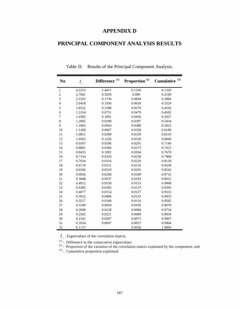
187
APPENDIX D
PRINCIPAL COMPONENT ANALYSIS RESULTS
Table D. Results of the Principal Component Analysis.
No iλ Difference (1) Proportion (2) Cumulative (3)
1 4.2253 1.4411 0.1320 0.1320 2 2.7841 0.5639 0.080 0.2190 3 2.2202 0.1744 0.0694 0.2884 4 2.0458 0.1936 0.0639 0.3524 5 1.8522 0.3188 0.0579 0.4102 6 1.5334 0.0751 0.0479 0.4582 7 1.4583 0.1891 0.0456 0.5037 8 1.2692 0.0290 0.0397 0.5434 9 1.2402 0.0943 0.0388 0.5822 10 1.1458 0.0607 0.0358 0.6180 11 1.0851 0.0288 0.0339 0.6519 12 1.0563 0.1256 0.0330 0.6849 13 0.9307 0.0506 0.0291 0.7140 14 0.8801 0.0366 0.0275 0.7415 15 0.8435 0.1081 0.0264 0.7678 16 0.7354 0.0320 0.0230 0.7908 17 0.7034 0.0316 0.0220 0.8128 18 0.6718 0.0151 0.0210 0.8338 19 0.6566 0.0510 0.0205 0.8543 20 0.6056 0.0208 0.0189 0.8732 21 0.5848 0.0937 0.0183 0.8915 22 0.4912 0.0530 0.0153 0.9068 23 0.4382 0.0305 0.0137 0.9205 24 0.4077 0.0154 0.0127 0.9333 25 0.3922 0.0406 0.0123 0.9455 26 0.3517 0.0168 0.0110 0.9565 27 0.3349 0.0659 0.0105 0.9670 28 0.2690 0.0128 0.0084 0.9754 29 0.2562 0.0221 0.0080 0.9834 30 0.2341 0.0507 0.0073 0.9907 31 0.1834 0.0697 0.0057 0.9964 32 0.1137 0.0036 1.0000
iλ : Eigenvalues of the correlation matrix;
(1) : Difference in the consecutive eigenvalues (2) : Proportion of the variation of the correlation matrix explained by the component; and (3) : Cumulative proportion explained.
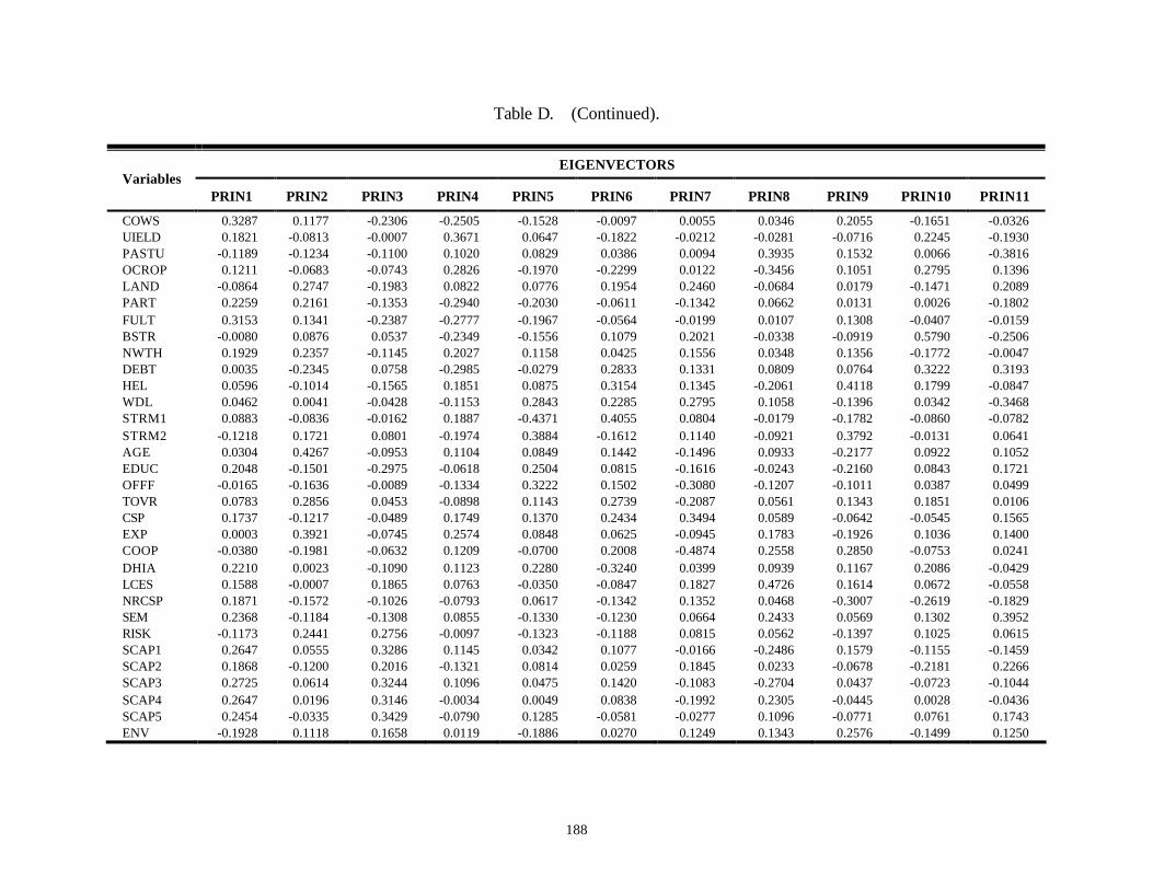
188
Table D. (Continued).
EIGENVECTORS Variables
PRIN1 PRIN2 PRIN3 PRIN4 PRIN5 PRIN6 PRIN7 PRIN8 PRIN9 PRIN10 PRIN11
COWS 0.3287 0.1177 -0.2306 -0.2505 -0.1528 -0.0097 0.0055 0.0346 0.2055 -0.1651 -0.0326 UIELD 0.1821 -0.0813 -0.0007 0.3671 0.0647 -0.1822 -0.0212 -0.0281 -0.0716 0.2245 -0.1930 PASTU -0.1189 -0.1234 -0.1100 0.1020 0.0829 0.0386 0.0094 0.3935 0.1532 0.0066 -0.3816 OCROP 0.1211 -0.0683 -0.0743 0.2826 -0.1970 -0.2299 0.0122 -0.3456 0.1051 0.2795 0.1396 LAND -0.0864 0.2747 -0.1983 0.0822 0.0776 0.1954 0.2460 -0.0684 0.0179 -0.1471 0.2089 PART 0.2259 0.2161 -0.1353 -0.2940 -0.2030 -0.0611 -0.1342 0.0662 0.0131 0.0026 -0.1802 FULT 0.3153 0.1341 -0.2387 -0.2777 -0.1967 -0.0564 -0.0199 0.0107 0.1308 -0.0407 -0.0159 BSTR -0.0080 0.0876 0.0537 -0.2349 -0.1556 0.1079 0.2021 -0.0338 -0.0919 0.5790 -0.2506 NWTH 0.1929 0.2357 -0.1145 0.2027 0.1158 0.0425 0.1556 0.0348 0.1356 -0.1772 -0.0047 DEBT 0.0035 -0.2345 0.0758 -0.2985 -0.0279 0.2833 0.1331 0.0809 0.0764 0.3222 0.3193 HEL 0.0596 -0.1014 -0.1565 0.1851 0.0875 0.3154 0.1345 -0.2061 0.4118 0.1799 -0.0847 WDL 0.0462 0.0041 -0.0428 -0.1153 0.2843 0.2285 0.2795 0.1058 -0.1396 0.0342 -0.3468 STRM1 0.0883 -0.0836 -0.0162 0.1887 -0.4371 0.4055 0.0804 -0.0179 -0.1782 -0.0860 -0.0782 STRM2 -0.1218 0.1721 0.0801 -0.1974 0.3884 -0.1612 0.1140 -0.0921 0.3792 -0.0131 0.0641 AGE 0.0304 0.4267 -0.0953 0.1104 0.0849 0.1442 -0.1496 0.0933 -0.2177 0.0922 0.1052 EDUC 0.2048 -0.1501 -0.2975 -0.0618 0.2504 0.0815 -0.1616 -0.0243 -0.2160 0.0843 0.1721 OFFF -0.0165 -0.1636 -0.0089 -0.1334 0.3222 0.1502 -0.3080 -0.1207 -0.1011 0.0387 0.0499 TOVR 0.0783 0.2856 0.0453 -0.0898 0.1143 0.2739 -0.2087 0.0561 0.1343 0.1851 0.0106 CSP 0.1737 -0.1217 -0.0489 0.1749 0.1370 0.2434 0.3494 0.0589 -0.0642 -0.0545 0.1565 EXP 0.0003 0.3921 -0.0745 0.2574 0.0848 0.0625 -0.0945 0.1783 -0.1926 0.1036 0.1400 COOP -0.0380 -0.1981 -0.0632 0.1209 -0.0700 0.2008 -0.4874 0.2558 0.2850 -0.0753 0.0241 DHIA 0.2210 0.0023 -0.1090 0.1123 0.2280 -0.3240 0.0399 0.0939 0.1167 0.2086 -0.0429 LCES 0.1588 -0.0007 0.1865 0.0763 -0.0350 -0.0847 0.1827 0.4726 0.1614 0.0672 -0.0558 NRCSP 0.1871 -0.1572 -0.1026 -0.0793 0.0617 -0.1342 0.1352 0.0468 -0.3007 -0.2619 -0.1829 SEM 0.2368 -0.1184 -0.1308 0.0855 -0.1330 -0.1230 0.0664 0.2433 0.0569 0.1302 0.3952 RISK -0.1173 0.2441 0.2756 -0.0097 -0.1323 -0.1188 0.0815 0.0562 -0.1397 0.1025 0.0615 SCAP1 0.2647 0.0555 0.3286 0.1145 0.0342 0.1077 -0.0166 -0.2486 0.1579 -0.1155 -0.1459 SCAP2 0.1868 -0.1200 0.2016 -0.1321 0.0814 0.0259 0.1845 0.0233 -0.0678 -0.2181 0.2266 SCAP3 0.2725 0.0614 0.3244 0.1096 0.0475 0.1420 -0.1083 -0.2704 0.0437 -0.0723 -0.1044 SCAP4 0.2647 0.0196 0.3146 -0.0034 0.0049 0.0838 -0.1992 0.2305 -0.0445 0.0028 -0.0436 SCAP5 0.2454 -0.0335 0.3429 -0.0790 0.1285 -0.0581 -0.0277 0.1096 -0.0771 0.0761 0.1743 ENV -0.1928 0.1118 0.1658 0.0119 -0.1886 0.0270 0.1249 0.1343 0.2576 -0.1499 0.1250
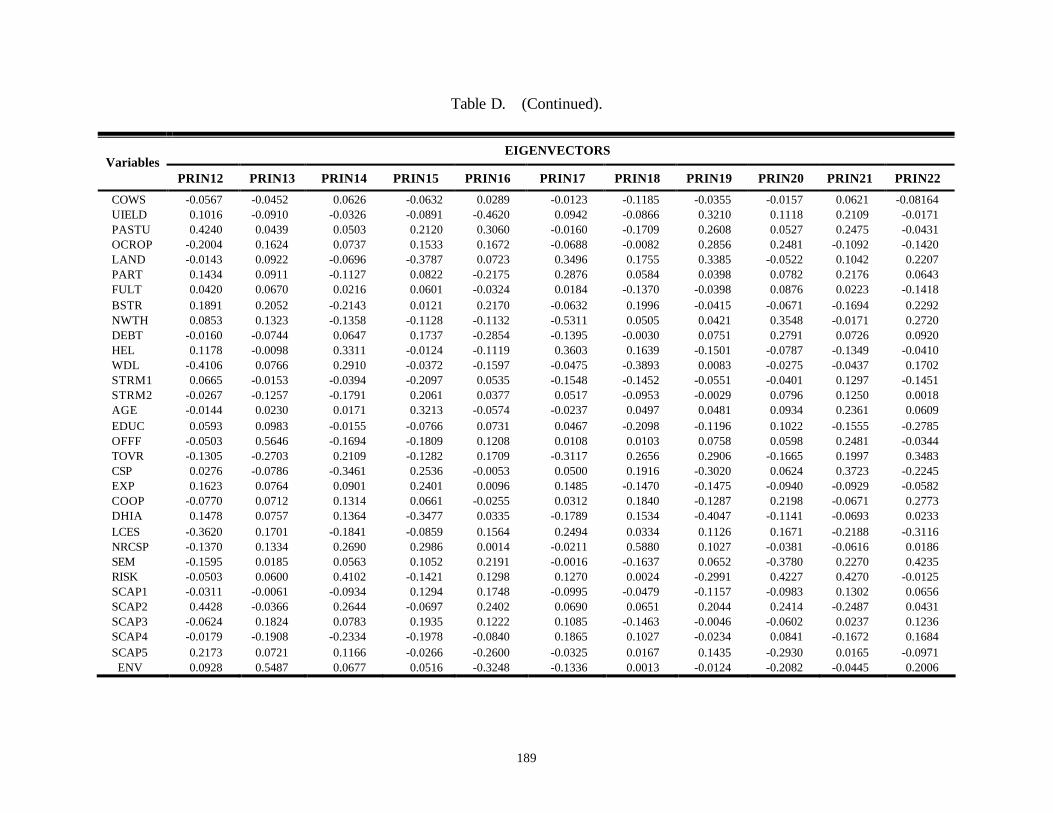
189
Table D. (Continued).
EIGENVECTORS Variables
PRIN12 PRIN13 PRIN14 PRIN15 PRIN16 PRIN17 PRIN18 PRIN19 PRIN20 PRIN21 PRIN22
COWS -0.0567 -0.0452 0.0626 -0.0632 0.0289 -0.0123 -0.1185 -0.0355 -0.0157 0.0621 -0.08164 UIELD 0.1016 -0.0910 -0.0326 -0.0891 -0.4620 0.0942 -0.0866 0.3210 0.1118 0.2109 -0.0171 PASTU 0.4240 0.0439 0.0503 0.2120 0.3060 -0.0160 -0.1709 0.2608 0.0527 0.2475 -0.0431 OCROP -0.2004 0.1624 0.0737 0.1533 0.1672 -0.0688 -0.0082 0.2856 0.2481 -0.1092 -0.1420 LAND -0.0143 0.0922 -0.0696 -0.3787 0.0723 0.3496 0.1755 0.3385 -0.0522 0.1042 0.2207 PART 0.1434 0.0911 -0.1127 0.0822 -0.2175 0.2876 0.0584 0.0398 0.0782 0.2176 0.0643 FULT 0.0420 0.0670 0.0216 0.0601 -0.0324 0.0184 -0.1370 -0.0398 0.0876 0.0223 -0.1418 BSTR 0.1891 0.2052 -0.2143 0.0121 0.2170 -0.0632 0.1996 -0.0415 -0.0671 -0.1694 0.2292 NWTH 0.0853 0.1323 -0.1358 -0.1128 -0.1132 -0.5311 0.0505 0.0421 0.3548 -0.0171 0.2720 DEBT -0.0160 -0.0744 0.0647 0.1737 -0.2854 -0.1395 -0.0030 0.0751 0.2791 0.0726 0.0920 HEL 0.1178 -0.0098 0.3311 -0.0124 -0.1119 0.3603 0.1639 -0.1501 -0.0787 -0.1349 -0.0410 WDL -0.4106 0.0766 0.2910 -0.0372 -0.1597 -0.0475 -0.3893 0.0083 -0.0275 -0.0437 0.1702 STRM1 0.0665 -0.0153 -0.0394 -0.2097 0.0535 -0.1548 -0.1452 -0.0551 -0.0401 0.1297 -0.1451 STRM2 -0.0267 -0.1257 -0.1791 0.2061 0.0377 0.0517 -0.0953 -0.0029 0.0796 0.1250 0.0018 AGE -0.0144 0.0230 0.0171 0.3213 -0.0574 -0.0237 0.0497 0.0481 0.0934 0.2361 0.0609 EDUC 0.0593 0.0983 -0.0155 -0.0766 0.0731 0.0467 -0.2098 -0.1196 0.1022 -0.1555 -0.2785 OFFF -0.0503 0.5646 -0.1694 -0.1809 0.1208 0.0108 0.0103 0.0758 0.0598 0.2481 -0.0344 TOVR -0.1305 -0.2703 0.2109 -0.1282 0.1709 -0.3117 0.2656 0.2906 -0.1665 0.1997 0.3483 CSP 0.0276 -0.0786 -0.3461 0.2536 -0.0053 0.0500 0.1916 -0.3020 0.0624 0.3723 -0.2245 EXP 0.1623 0.0764 0.0901 0.2401 0.0096 0.1485 -0.1470 -0.1475 -0.0940 -0.0929 -0.0582 COOP -0.0770 0.0712 0.1314 0.0661 -0.0255 0.0312 0.1840 -0.1287 0.2198 -0.0671 0.2773 DHIA 0.1478 0.0757 0.1364 -0.3477 0.0335 -0.1789 0.1534 -0.4047 -0.1141 -0.0693 0.0233 LCES -0.3620 0.1701 -0.1841 -0.0859 0.1564 0.2494 0.0334 0.1126 0.1671 -0.2188 -0.3116 NRCSP -0.1370 0.1334 0.2690 0.2986 0.0014 -0.0211 0.5880 0.1027 -0.0381 -0.0616 0.0186 SEM -0.1595 0.0185 0.0563 0.1052 0.2191 -0.0016 -0.1637 0.0652 -0.3780 0.2270 0.4235 RISK -0.0503 0.0600 0.4102 -0.1421 0.1298 0.1270 0.0024 -0.2991 0.4227 0.4270 -0.0125 SCAP1 -0.0311 -0.0061 -0.0934 0.1294 0.1748 -0.0995 -0.0479 -0.1157 -0.0983 0.1302 0.0656 SCAP2 0.4428 -0.0366 0.2644 -0.0697 0.2402 0.0690 0.0651 0.2044 0.2414 -0.2487 0.0431 SCAP3 -0.0624 0.1824 0.0783 0.1935 0.1222 0.1085 -0.1463 -0.0046 -0.0602 0.0237 0.1236 SCAP4 -0.0179 -0.1908 -0.2334 -0.1978 -0.0840 0.1865 0.1027 -0.0234 0.0841 -0.1672 0.1684 SCAP5 0.2173 0.0721 0.1166 -0.0266 -0.2600 -0.0325 0.0167 0.1435 -0.2930 0.0165 -0.0971 ENV 0.0928 0.5487 0.0677 0.0516 -0.3248 -0.1336 0.0013 -0.0124 -0.2082 -0.0445 0.2006
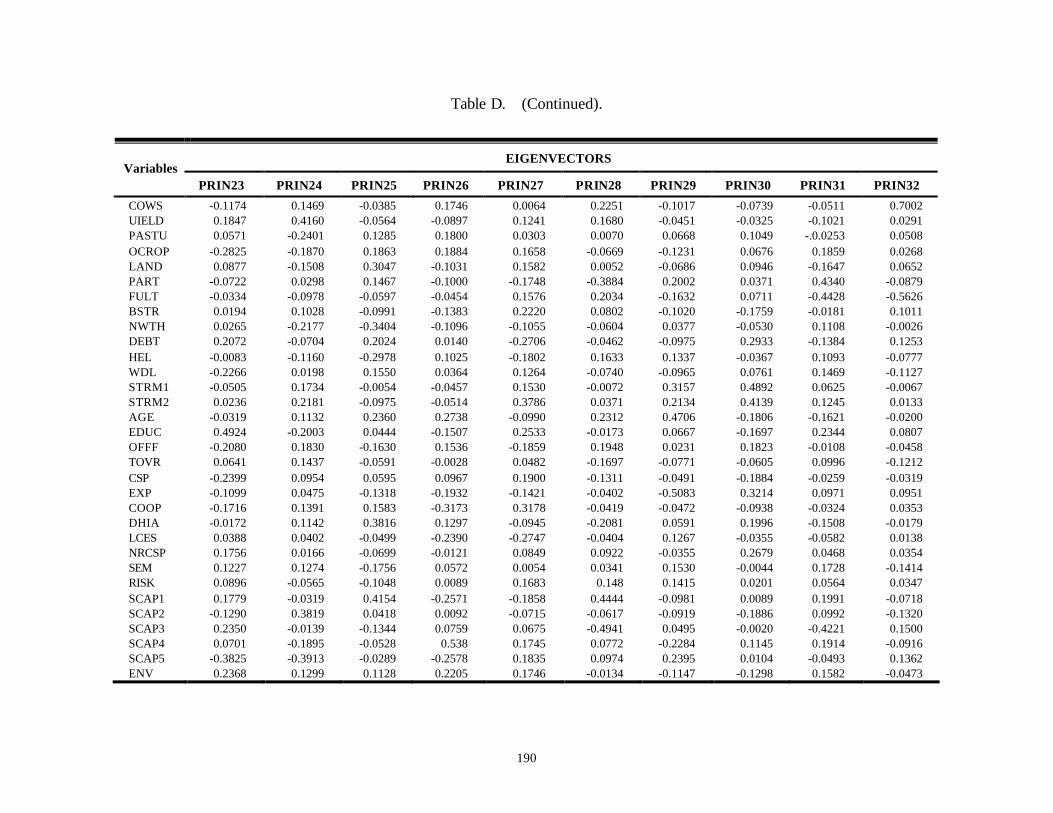
190
Table D. (Continued).
EIGENVECTORS Variables
PRIN23 PRIN24 PRIN25 PRIN26 PRIN27 PRIN28 PRIN29 PRIN30 PRIN31 PRIN32
COWS -0.1174 0.1469 -0.0385 0.1746 0.0064 0.2251 -0.1017 -0.0739 -0.0511 0.7002 UIELD 0.1847 0.4160 -0.0564 -0.0897 0.1241 0.1680 -0.0451 -0.0325 -0.1021 0.0291 PASTU 0.0571 -0.2401 0.1285 0.1800 0.0303 0.0070 0.0668 0.1049 -.0.0253 0.0508 OCROP -0.2825 -0.1870 0.1863 0.1884 0.1658 -0.0669 -0.1231 0.0676 0.1859 0.0268 LAND 0.0877 -0.1508 0.3047 -0.1031 0.1582 0.0052 -0.0686 0.0946 -0.1647 0.0652 PART -0.0722 0.0298 0.1467 -0.1000 -0.1748 -0.3884 0.2002 0.0371 0.4340 -0.0879 FULT -0.0334 -0.0978 -0.0597 -0.0454 0.1576 0.2034 -0.1632 0.0711 -0.4428 -0.5626 BSTR 0.0194 0.1028 -0.0991 -0.1383 0.2220 0.0802 -0.1020 -0.1759 -0.0181 0.1011 NWTH 0.0265 -0.2177 -0.3404 -0.1096 -0.1055 -0.0604 0.0377 -0.0530 0.1108 -0.0026 DEBT 0.2072 -0.0704 0.2024 0.0140 -0.2706 -0.0462 -0.0975 0.2933 -0.1384 0.1253 HEL -0.0083 -0.1160 -0.2978 0.1025 -0.1802 0.1633 0.1337 -0.0367 0.1093 -0.0777 WDL -0.2266 0.0198 0.1550 0.0364 0.1264 -0.0740 -0.0965 0.0761 0.1469 -0.1127 STRM1 -0.0505 0.1734 -0.0054 -0.0457 0.1530 -0.0072 0.3157 0.4892 0.0625 -0.0067 STRM2 0.0236 0.2181 -0.0975 -0.0514 0.3786 0.0371 0.2134 0.4139 0.1245 0.0133 AGE -0.0319 0.1132 0.2360 0.2738 -0.0990 0.2312 0.4706 -0.1806 -0.1621 -0.0200 EDUC 0.4924 -0.2003 0.0444 -0.1507 0.2533 -0.0173 0.0667 -0.1697 0.2344 0.0807 OFFF -0.2080 0.1830 -0.1630 0.1536 -0.1859 0.1948 0.0231 0.1823 -0.0108 -0.0458 TOVR 0.0641 0.1437 -0.0591 -0.0028 0.0482 -0.1697 -0.0771 -0.0605 0.0996 -0.1212 CSP -0.2399 0.0954 0.0595 0.0967 0.1900 -0.1311 -0.0491 -0.1884 -0.0259 -0.0319 EXP -0.1099 0.0475 -0.1318 -0.1932 -0.1421 -0.0402 -0.5083 0.3214 0.0971 0.0951 COOP -0.1716 0.1391 0.1583 -0.3173 0.3178 -0.0419 -0.0472 -0.0938 -0.0324 0.0353 DHIA -0.0172 0.1142 0.3816 0.1297 -0.0945 -0.2081 0.0591 0.1996 -0.1508 -0.0179 LCES 0.0388 0.0402 -0.0499 -0.2390 -0.2747 -0.0404 0.1267 -0.0355 -0.0582 0.0138 NRCSP 0.1756 0.0166 -0.0699 -0.0121 0.0849 0.0922 -0.0355 0.2679 0.0468 0.0354 SEM 0.1227 0.1274 -0.1756 0.0572 0.0054 0.0341 0.1530 -0.0044 0.1728 -0.1414 RISK 0.0896 -0.0565 -0.1048 0.0089 0.1683 0.148 0.1415 0.0201 0.0564 0.0347 SCAP1 0.1779 -0.0319 0.4154 -0.2571 -0.1858 0.4444 -0.0981 0.0089 0.1991 -0.0718 SCAP2 -0.1290 0.3819 0.0418 0.0092 -0.0715 -0.0617 -0.0919 -0.1886 0.0992 -0.1320 SCAP3 0.2350 -0.0139 -0.1344 0.0759 0.0675 -0.4941 0.0495 -0.0020 -0.4221 0.1500 SCAP4 0.0701 -0.1895 -0.0528 0.538 0.1745 0.0772 -0.2284 0.1145 0.1914 -0.0916 SCAP5 -0.3825 -0.3913 -0.0289 -0.2578 0.1835 0.0974 0.2395 0.0104 -0.0493 0.1362 ENV 0.2368 0.1299 0.1128 0.2205 0.1746 -0.0134 -0.1147 -0.1298 0.1582 -0.0473

191
APPENDIX E
PROBIT ANALYSIS WITH 30 VARIABLES
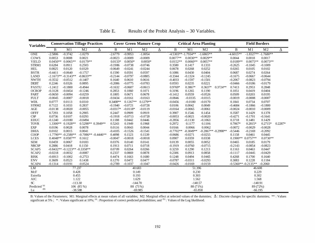
192
Table E. Results of the Probit Analysis – 30 Variables.
Conservation Tillage Practices Cover Green Manure Crop Critical Area Planting Field Borders Variables B M1 M2 ∆ B M1 M2 ∆ B M1 M2 ∆ B M1 M2 ∆
ONE -2.5806 -0.3742 -1.0279 -2.6779 -0.9953 -1.0054 -4.5303** -1.7934** -1.6865** -4.6015** -1.8327** -1.7680** COWS 0.0053 0.0008 0.0021 -0.0023 -0.0009 -0.0009 0.0077** 0.0030** 0.0029** 0.0044 0.0018 0.0017 YIELD 0.0450** 0.0065** 0.0179** 0.0133* 0.0050* 0.0050* 0.0152** 0.0060** 0.0057** 0.0189** 0.0075** 0.0073** STRM1 0.6284 0.0911 0.2503 -0.1986 -0.0738 -0.0746 0.3580 0.1417 0.1333 -0.2625 -0.1045 -0.1009 HEL 0.0825 0.0120 0.0329 -0.0649 -0.0241 -0.0244 0.0678 0.0268 0.0252 0.0265 0.0105 0.0102 BSTR -0.4411 -0.0640 -0.1757 0.1590 0.0591 0.0597 0.1086 0.0430 0.0404 0.0687 0.0274 0.0264 LAND -2.1673** -0.3143** -0.8633** -0.2144 -0.0797 -0.0805 -0.3344 -0.1324 -0.1245 -0.1675 -0.0667 -0.0644 NWTH -0.3532 -0.0512 -0.1407 0.1640 0.0610 0.0616 -0.4033 -0.1597 -0.1501 -0.2067 -0.0823 -0.0794 DEBT 0.2246 0.0326 0.0895 -0.2086 -0.0775 -0.0783 0.0593 0.0235 0.0221 -0.0466 -0.0186 -0.0179 PASTU -1.2412 -0.1800 -0.4944 -0.1632 -0.0607 -0.0613 0.9769* 0.3867* 0.3637* 0.3724** 0.7413 0.2953 0.2848 OCROP -0.3128 -0.0454 -0.1246 0.2853 0.1060 0.1071 0.3196 0.1265 0.1190 0.1051 0.0419 0.0404 PART -0.0650 -0.0094 -0.0259 0.1805 0.0671 0.0678 -0.1412 0.0559 -0.0526 0.0509 0.0203 0.0195 FULT -0.0045 -0.0007 -0.0018 -0.0434 -0.0161 -0.0163 -0.0846 -0.0335 -0.0315 -0.0019 -0.0008 -0.0007 WDL 0.0777 0.0113 0.0310 0.3408** 0.1267** 0.1279** -0.0456 -0.0180 -0.0170 0.1841 0.0734 0.0707 STRM2 0.7122 0.1033 0.2837 -0.1940 -0.0721 -0.0728 0.0106 0.0042 0.0049 -0.4684 -0.1866 -0.1800 AGE -0.0138 -0.0020 -0.0055 -0.0317* -0.0118* -0.0119 -0.0164 -0.0065 -0.0061 -0.0024 -0.0010 -0.0009 OFFF 0.7293 0.1058 0.2905 0.2447 0.0909 0.0919 0.3907 0.1546 0.1454 0.3587 0.1429 0.1378 CSP 0.0736 0.0107 0.0293 -0.1918 -0.0713 -0.0720 -0.0053 -0.0021 -0.0020 -0.4271 -0.1701 -0.1641 EDUC -0.1240 -0.0180 -0.0494 0.1188 0.0442 0.0446 -0.2856 -0.1130 -0.1063 0.3718 0.1481 0.1429 TOVR 1.3300** 0.1928** 0.5298** 0.3949** 0.5243 0.1949 0.1968 0.2972 0.1177 0.1106 0.7067* 0.2815* 0.2715* 0.2287* EXP 0.0196 0.0028 0.0078 0.0116 0.0043 0.0044 0.0166 0.0066 0.0062 -0.0072 -0.0029 -0.0028 DHIA 0.0102 0.0015 0.0041 -0.4105 -0.1526 -0.1541 -0.7702** -0.3049** -0.2867** -0.2998** -0.5446 -0.2169 -0.2092 COOP -1.7790** -0.2580** -0.7086** -0.4446** 0.4098 0.1523 0.1539 -0.0686 -0.0271 -0.0255 0.1158 0.0461 0.0445 LCES 0.4048** 0.0587** 0.1612 -0.0047 -0.0018 -0.0018 0.0907 0.0359 0.0338 0.1900** 0.0757** 0.0730** SEM 0.0459 0.0067 0.0183 0.0376 0.0140 0.0141 0.0139 0.0055 0.0052 0.0465 0.0185 0.0179 NRCSP 0.2886 0.0418 0.1150 0.1913 0.0711 0.0718 -0.1919 -0.0760 -0.0715 -0.2143 -0.0854 -0.0823 SCAP5 -0.8432** -0.1223** -0.3358** 0.0709 0.0264 0.0266 0.3259 0.1290 0.1213 0.1163 0.0463 0.0447 SCAP2 -0.0218 -0.0032 -0.0087 0.2337 0.0869 0.0878 0.2306 0.0913 0.0858 -0.1117 -0.0445 -0.0429 RISK -0.6913 -0.1002 -0.2753 0.4474 0.1663 0.1680 0.1248 0.0494 0.0465 0.4268 0.1700 0.1640 ENV 0.3609 0.0523 0.1438 0.1270 0.0472 0.0477 -0.0787 -0.0311 -0.0293 0.3083 0.1228 0.1184 SCAP4 -0.1314 -0.0191 -0.0524 -0.2789 -0.1037 -0.1047 -0.0426 -0.0169 -0.0159 -0.5360** -0.2135** -0.2060 LM 77.237 40.683 51.396 46.608 McF 0.428 0.149 0.230 0.229 Estrella 0.455 0.193 0.303 0.302 AIC 1.122 1.629 1.562 1.568 SC -113.30 -144.70 -140.57 -140.91
Predicted (a) 106 (85 %) 88 (71%) 88 (71%) 89 (72%) Lu (B) -38.588 -69.985 -65.858 -66.195
B: Values of the Parameters; M1: Marginal effects at mean values of all variables; M2: Marginal effect at selected values of the dummies; ∆ : Discrete changes for specific dummies; ** : Values significant at 5% ; * : Values significant at 10%; (a) : Proportion of correct predicted probabilities; and (b) : Values of the Log likelihood.
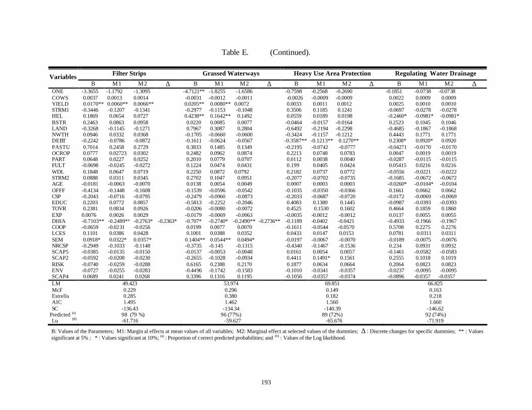
193
Table E. (Continued).
Filter Strips Grassed Waterways Heavy Use Area Protection Regulating Water Drainage Variables B M1 M2 ∆ B M1 M2 ∆ B M1 M2 ∆ B M1 M2 ∆
ONE -3.3655 -1.1792 -1.3095 -4.7121** -1.8255 -1.6586 -0.7598 -0.2568 -0.2690 -0.1851 -0.0738 -0.0738 COWS 0.0037 0.0013 0.0014 -0.0031 -0.0012 -0.0011 -0.0026 -0.0009 -0.0009 0.0022 0.0009 0.0009 YIELD 0.0170** 0.0060** 0.0066** 0.0205** 0.0080** 0.0072 0.0033 0.0011 0.0012 0.0025 0.0010 0.0010 STRM1 -0.3446 -0.1207 -0.1341 -0.2977 -0.1153 -0.1048 0.3506 0.1185 0.1241 -0.0697 -0.0278 -0.0278 HEL 0.1869 0.0654 0.0727 0.4238** 0.1642** 0.1492 0.0559 0.0189 0.0198 -0.2460* -0.0981* -0.0981* BSTR 0.2463 0.0863 0.0958 0.0220 0.0085 0.0077 -0.0464 -0.0157 -0.0164 0.2523 0.1045 0.1046 LAND -0.3268 -0.1145 -0.1271 0.7967 0.3087 0.2804 -0.6492 -0.2194 -0.2298 -0.4685 -0.1867 -0.1868 NWTH 0.0946 0.0332 0.0368 -0.1705 -0.0660 -0.0600 -0.3424 -0.1157 -0.1212 0.4443 0.1771 0.1771 DEBT -0.2242 -0.0786 -0.0872 -0.1611 -0.0624 -0.0567 -0.3587** -0.1213** 0.1270** 0.2308* 0.0920* 0.0920 PASTU 0.7014 0.2458 0.2729 0.3833 0.1485 0.1349 -0.2195 -0.0742 -0.0777 -0.04271 -0.0170 -0.0170 OCROP 0.0777 0.02723 0.0302 0.2482 0.0962 0.0874 0.2213 0.0748 0.0783 0.0047 0.0019 0.0019 PART 0.0648 0.0227 0.0252 0.2010 0.0779 0.0707 0.0112 0.0038 0.0040 -0.0287 -0.0115 -0.0115 FULT -0.0698 -0.0245 -0.0272 0.1224 0.0474 0.0431 0.199 0.0405 0.0424 0.05415 0.0216 0.0216 WDL 0.1848 0.0647 0.0719 0.2250 0.0872 0.0792 0.2182 0.0737 0.0772 -0.0556 -0.0221 -0.0222 STRM2 0.0888 0.0311 0.0345 0.2702 0.1047 0.0951 -0.2077 -0.0702 -0.0735 -0.1685 -0.0672 -0.0672 AGE -0.0181 -0.0063 -0.0070 0.0138 0.0054 0.0049 0.0007 0.0003 0.0003 -0.0260* -0.0104* -0.0104 OFFF -0.4134 -0.1448 -0.1608 -0.1539 -0.0596 -0.0542 -0.1035 -0.0350 -0.0366 0.1661 0.0662 0.0662 CSP -0.2043 -0.0716 -0.0795 -0.2479 -0.0960 -0.0873 -0.2033 -0.0687 -0.0720 -0.0172 -0.0069 -0.0069 EDUC 0.2203 0.0772 0.0857 -0.5813 -0.2252 -0.2046 0.4083 0.1380 0.1445 -0.0987 -0.0393 -0.0393 TOVR 0.2381 0.0834 0.0926 -0.0206 -0.0080 -0.0072 0.4525 0.1530 0.1602 0.4664 0.1859 0.1860 EXP 0.0076 0.0026 0.0029 -0.0179 -0.0069 -0.0063 -0.0035 -0.0012 -0.0012 0.0137 0.0055 0.0055 DHIA -0.7103** -0.2489** -0.2763* -0.2363* -0.707* -0.2740* -0.2490** -0.2736** -0.1189 -0.0402 -0.0421 -0.4933 -0.1966 -0.1967 COOP -0.0659 -0.0231 -0.0256 0.0199 0.0077 0.0070 -0.1611 -0.0544 -0.0570 0.5708 0.2275 0.2276 LCES 0.1101 0.0386 0.0428 0.1001 0.0388 0.0352 0.0433 0.0147 0.0153 0.0781 0.0311 0.0311 SEM 0.0918* 0.0322* 0.0357* 0.1404** 0.0544** 0.0494* -0.0197 -0.0067 -0.0070 -0.0189 -0.0075 -0.0076 NRCSP -0.2949 -0.1033 -0.1148 -0.3735 -0.145 -0.1315 -0.4340 -0.1467 -0.1536 0.234 0.0931 0.0932 SCAP5 -0.0385 -0.0135 -0.0150 -0.0137 -0.0053 -0.0048 0.0161 0.0054 0.0057 -0.1461 -0.0582 -0.0583 SCAP2 -0.0592 -0.0208 -0.0230 -0.2655 -0.1028 -0.0934 0.4411 0.1491* 0.1561 0.2555 0.1018 0.1019 RISK -0.0740 -0.0259 -0.0288 0.6165 0.2388 0.2170 0.1877 0.0634 0.0664 0.2064 0.0823 0.0823 ENV -0.0727 -0.0255 -0.0283 -0.4496 -0.1742 -0.1583 -0.1010 -0.0341 -0.0357 -0.0237 -0.0095 -0.0095 SCAP4 0.0689 0.0241 0.0268 0.3396 0.1316 0.1195 -0.1056 -0.0357 -0.0374 -0.0896 -0.0357 -0.0357 LM 49.423 53.974 69.851 66.825 McF 0.229 0.296 0.149 0.163 Estrella 0.285 0.380 0.182 0.218 AIC 1.495 1.462 1.560 1.660 SC -136.43 -134.34 -140.39 -146.62
Predicted (a) 98 (79 %) 96 (77%) 89 (72%) 92 (74%) Lu (B) -61.716 -59.627 -65.676 -71.919
B: Values of the Parameters; M1: Margin al effects at mean values of all variables; M2: Marginal effect at selected values of the dummies; ∆ : Discrete changes for specific dummies; ** : Values significant at 5% ; * : Values significant at 10%; (a) : Proportion of correct predicted probabilities; and (b) : Values of the Log likelihood.
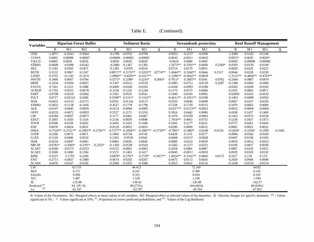
194
Table E. (Continued).
Riparian Forest Buffer Sediment Basin Streambank protection Roof Runoff Management Variables B M1 M2 ∆ B M1 M2 ∆ B M1 M2 ∆ B M1 M2 ∆
ONE -1.4071 -0.4343 -0.5604 -0.1786 -0.0702 -0.0709 -0.9053 -0.2157 -0.0390 -1.4389 -0.5102 -0.5146 COWS 0.0002 0.00006 0.00007 -0.00006 -0.00002 -0.00002 -0.0045 -0.0011 -0.0002 0.0055* 0.0020 0.0020* YIELD 0.0065 0.0020 0.0026 0.0050 0.0020 0.0020 0.0024 0.0006 0.0001 -0.0002 -0.00008 -0.00008 STRM1 -0.0608 -0.0188 -0.0242 -0.3480 -0.1367 -0.1381 1.5073** 0.3591** 0.0649 0.2560* -0.0393 -0.0139 -0.0140 HEL 0.1182 0.0365 0.0471 0.1285 0.0505 0.0510 0.0714 0.0170 0.0031 0.0620 0.0220 0.0222 BSTR 0.3132 0.0967 0.1247 0.8071** 0.3170** 0.3203** 02774** 1.4944** 0.3560** 0.0644 0.2517 0.0644 0.0228 0.0230 LAND -0.3701 -0.1142 -0.1474 -1.0904** -0.4283** -0.4327** -1.5286** -0.3642** -0.0659 -1.3152** -0.4664** -0.4703** NWTH 0.1968 0.0607 0.0784 0.5571* 0.2188* 0.2210* 0.2043* 0.7911* 0.1885** 0.0341 0.0762 -0.2444 -0.0867 -0.0874 DEBT -0.1634 -0.0504 -0.0651 -0.1307 -0.0513 -0.0519 -0.2983 -0.0711 -0.0129 0.2587 -0.1386 -0.0492 -0.0496 PASTU 0.7501 0.2315 0.2988 -0.0409 -0.0160 -0.0162 -0.4166 -0.0993 -0.0180 -0.0565 -0.0200 -0.0202 OCROP -0.1702 -0.0525 -0.0678 -0.3136 -0.1232 -0.1244 0.1573 0.0375 0.0068 0.2435 0.0863 0.0871 PART -0.0708 -0.0219 -0.0282 0.1363 0.0535 0.0541 0.1449 0.0345 0.0062 -0.02859 -0.0101 -0.0102 FULT 0.0717 0.02214 0.0286 0.3338** 0.1311* 0.1324** -0.4411** -0.1051** -0.0190 -0.1403 -0.0498 -0.0502 WDL -0.0431 -0.0133 -0.0172 0.0291 0.01142 0.0115 0.0193 0.0046 0.0008 0.0667 0.0237 0.0239 STRM2 -0.3655 -0.1128 -0.1456 -0.4527 -0.1778 -0.1796 0.7258 0.1729 0.0313 0.1870 0.0663 0.0669 AGE -0.0147 -0.0045 -0.0059 -0.0214 -0.0084 -0.0085 -0.0517** -0.0123** -0.0022 -0.0012 -0.0004 -0.0004 OFFF -0.0233 -0.0072 -0.0093 0.5527 0.2171 0.2193 0.1854 0.0442 0.0080 0.4108 0.1457 0.1469 CSP -0.0184 -0.0057 -0.0073 0.1177 0.0462 0.0467 -0.1470 -0.0350 -0.0063 -0.1453 -0.0515 -0.0520 EDUC 0.3305 0.1020 0.1316 0.2136 0.0839 0.0848 1.7054** 0.4063 0.0735 0.5238 0.1857 0.1873 TOVR 0.0506 0.0156 0.0202 0.3645 0.1432 0.1446 0.5362 0.1277 0.0231 0.0737 0.0261 0.0264 EXP 0.0078 0.0024 0.0031 -0.0129 -0.0051 -0.0051 0.0290 0.0069 0.0012 0.0062 0.0022 0.0022 DHIA -0.7518** -0.2321** -0.2995** -0.2792** -0.7277** -0.2858** -0.2887** -0.2750** -0.7901* -0.1882* -0.0340 -0.0156 -0.5454* -0.1934* -0.1950 -0.1645 COOP 0.2186 0.0675 0.0871 0.1869 0.0734 0.0742 0.6428 0.1531 0.0277 -0.0966 -0.0342 -0.0345 LCES 0.1316 0.0406 0.0524 0.1363 0.0536 0.0541 -0.0660 -0.0157 -0.0028 0.0447 0.0158 0.0160 SEM -0.0154 -0.0047 -0.0061 0.0066 0.0026 0.0026 0.0900 0.0214 0.0039 -0.0035 -0.0012 -0.0013 NRCSP -0.6781* -0.2093* -0.2701* -0.2555* -0.1369 -0.0538 -0.0543 -0.5362 -0.1277 -0.0231 0.0106 0.0037 0.0038 SCAP5 -0.0560 -0.0173 -0.0223 -0.0155 -0.0061 -0.0062 0.2018 0.0481 0.0087 0.0897 0.0318 0.0321 SCAP2 0.3500 0.1080 0.1394 0.3572 0.1403 0.1417 -0.0045 -0.0011 -0.0002 0.0929 0.0329 0.0332 RISK 0.5525 0.1705 0.2200 0.6878* 0.2702* 0.2729* 0.2617** 1.4024** 0.3341** 0.0604 0.0172 0.3317 0.118 0.119 ENV -0.2711 -0.0837 -0.1080 -0.0674 -0.0265 -0.0267 0.0475 0.0113 0.0020 0.2650 0.0940 0.0948 SCAP4 0.0476 0.0147 0.0190 -0.2686 -0.1055 -0.1066 0.2653 0.0632 0.0114 -0.1438 -0.0510 -0.0514 LM 63.719 44.413 72.164 64.82 McF 0.171 0.247 0.380 0.145 Estrella 0.200 0.321 0.434 0.182 AIC 1.487 1.528 1.238 1.594 SC -135.88 -138.42 -120.48 -142.57
Predicted (a) 94 (76 %) 88 (71%) 104 (84%) 86 (69%) Lu (B) -61.167 -63.707 -45.764 -67.853
B: Values of the Parameters; M1: Marginal effects at mean values of all variables; M2: Marginal effect at selected values of the dummies; ∆ : Discrete changes for specific dummies; ** : Values significant at 5% ; * : Values significant at 10%; (a) : Proportion of correct predicted probabilities; and (b) : Values of the Log likelihood.
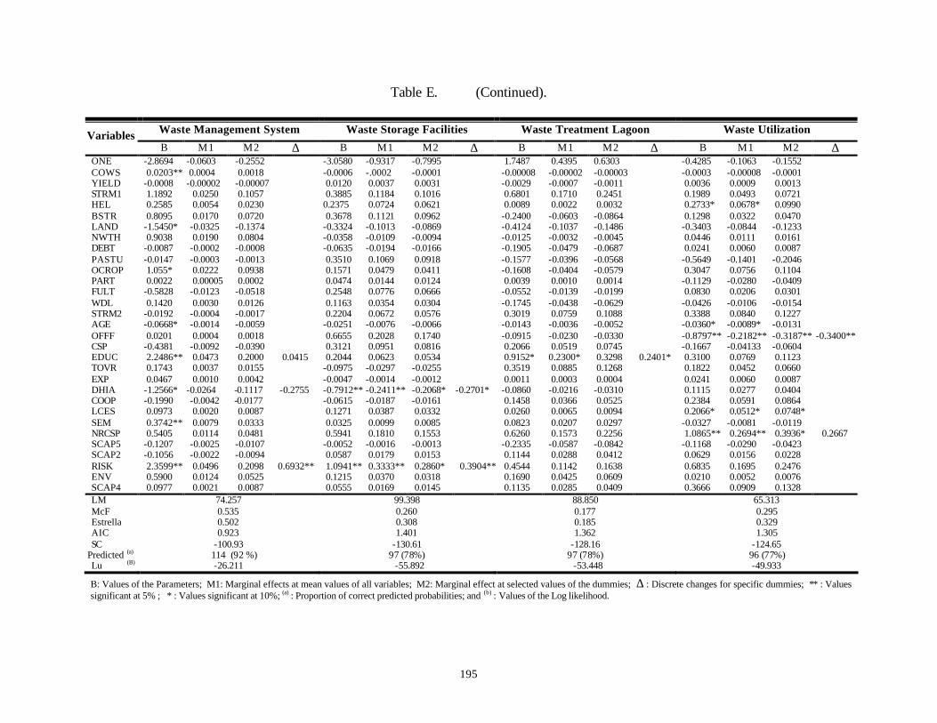
195
Table E. (Continued).
Waste Management System Waste Storage Facilities Waste Treatment Lagoon Waste Utilization Variables B M1 M2 ∆ B M1 M2 ∆ B M1 M2 ∆ B M1 M2 ∆
ONE -2.8694 -0.0603 -0.2552 -3.0580 -0.9317 -0.7995 1.7487 0.4395 0.6303 -0.4285 -0.1063 -0.1552 COWS 0.0203** 0.0004 0.0018 -0.0006 -.0002 -0.0001 -0.00008 -0.00002 -0.00003 -0.0003 -0.00008 -0.0001 YIELD -0.0008 -0.00002 -0.00007 0.0120 0.0037 0.0031 -0.0029 -0.0007 -0.0011 0.0036 0.0009 0.0013 STRM1 1.1892 0.0250 0.1057 0.3885 0.1184 0.1016 0.6801 0.1710 0.2451 0.1989 0.0493 0.0721 HEL 0.2585 0.0054 0.0230 0.2375 0.0724 0.0621 0.0089 0.0022 0.0032 0.2733* 0.0678* 0.0990 BSTR 0.8095 0.0170 0.0720 0.3678 0.1121 0.0962 -0.2400 -0.0603 -0.0864 0.1298 0.0322 0.0470 LAND -1.5450* -0.0325 -0.1374 -0.3324 -0.1013 -0.0869 -0.4124 -0.1037 -0.1486 -0.3403 -0.0844 -0.1233 NWTH 0.9038 0.0190 0.0804 -0.0358 -0.0109 -0.0094 -0.0125 -0.0032 -0.0045 0.0446 0.0111 0.0161 DEBT -0.0087 -0.0002 -0.0008 -0.0635 -0.0194 -0.0166 -0.1905 -0.0479 -0.0687 0.0241 0.0060 0.0087 PASTU -0.0147 -0.0003 -0.0013 0.3510 0.1069 0.0918 -0.1577 -0.0396 -0.0568 -0.5649 -0.1401 -0.2046 OCROP 1.055* 0.0222 0.0938 0.1571 0.0479 0.0411 -0.1608 -0.0404 -0.0579 0.3047 0.0756 0.1104 PART 0.0022 0.00005 0.0002 0.0474 0.0144 0.0124 0.0039 0.0010 0.0014 -0.1129 -0.0280 -0.0409 FULT -0.5828 -0.0123 -0.0518 0.2548 0.0776 0.0666 -0.0552 -0.0139 -0.0199 0.0830 0.0206 0.0301 WDL 0.1420 0.0030 0.0126 0.1163 0.0354 0.0304 -0.1745 -0.0438 -0.0629 -0.0426 -0.0106 -0.0154 STRM2 -0.0192 -0.0004 -0.0017 0.2204 0.0672 0.0576 0.3019 0.0759 0.1088 0.3388 0.0840 0.1227 AGE -0.0668* -0.0014 -0.0059 -0.0251 -0.0076 -0.0066 -0.0143 -0.0036 -0.0052 -0.0360* -0.0089* -0.0131 OFFF 0.0201 0.0004 0.0018 0.6655 0.2028 0.1740 -0.0915 -0.0230 -0.0330 -0.8797** -0.2182** -0.3187** -0.3400** CSP -0.4381 -0.0092 -0.0390 0.3121 0.0951 0.0816 0.2066 0.0519 0.0745 -0.1667 -0.04133 -0.0604 EDUC 2.2486** 0.0473 0.2000 0.0415 0.2044 0.0623 0.0534 0.9152* 0.2300* 0.3298 0.2401* 0.3100 0.0769 0.1123 TOVR 0.1743 0.0037 0.0155 -0.0975 -0.0297 -0.0255 0.3519 0.0885 0.1268 0.1822 0.0452 0.0660 EXP 0.0467 0.0010 0.0042 -0.0047 -0.0014 -0.0012 0.0011 0.0003 0.0004 0.0241 0.0060 0.0087 DHIA -1.2566* -0.0264 -0.1117 -0.2755 -0.7912** -0.2411** -0.2068* -0.2701* -0.0860 -0.0216 -0.0310 0.1115 0.0277 0.0404 COOP -0.1990 -0.0042 -0.0177 -0.0615 -0.0187 -0.0161 0.1458 0.0366 0.0525 0.2384 0.0591 0.0864 LCES 0.0973 0.0020 0.0087 0.1271 0.0387 0.0332 0.0260 0.0065 0.0094 0.2066* 0.0512* 0.0748* SEM 0.3742** 0.0079 0.0333 0.0325 0.0099 0.0085 0.0823 0.0207 0.0297 -0.0327 -0.0081 -0.0119 NRCSP 0.5405 0.0114 0.0481 0.5941 0.1810 0.1553 0.6260 0.1573 0.2256 1.0865** 0.2694** 0.3936* 0.2667 SCAP5 -0.1207 -0.0025 -0.0107 -0.0052 -0.0016 -0.0013 -0.2335 -0.0587 -0.0842 -0.1168 -0.0290 -0.0423 SCAP2 -0.1056 -0.0022 -0.0094 0.0587 0.0179 0.0153 0.1144 0.0288 0.0412 0.0629 0.0156 0.0228 RISK 2.3599** 0.0496 0.2098 0.6932** 1.0941** 0.3333** 0.2860* 0.3904** 0.4544 0.1142 0.1638 0.6835 0.1695 0.2476 ENV 0.5900 0.0124 0.0525 0.1215 0.0370 0.0318 0.1690 0.0425 0.0609 0.0210 0.0052 0.0076 SCAP4 0.0977 0.0021 0.0087 0.0555 0.0169 0.0145 0.1135 0.0285 0.0409 0.3666 0.0909 0.1328 LM 74.257 99.398 88.850 65.313 McF 0.535 0.260 0.177 0.295 Estrella 0.502 0.308 0.185 0.329 AIC 0.923 1.401 1.362 1.305 SC -100.93 -130.61 -128.16 -124.65
Predicted (a) 114 (92 %) 97 (78%) 97 (78%) 96 (77%) Lu (B) -26.211 -55.892 -53.448 -49.933
B: Values of the Parameters; M1: Marginal effects at mean values of all variables; M2: Marginal effect at selected values of the dummies; ∆ : Discrete changes for specific dummies; ** : Values significant at 5% ; * : Values significant at 10%; (a) : Proportion of correct predicted probabilities; and (b) : Values of the Log likelihood.
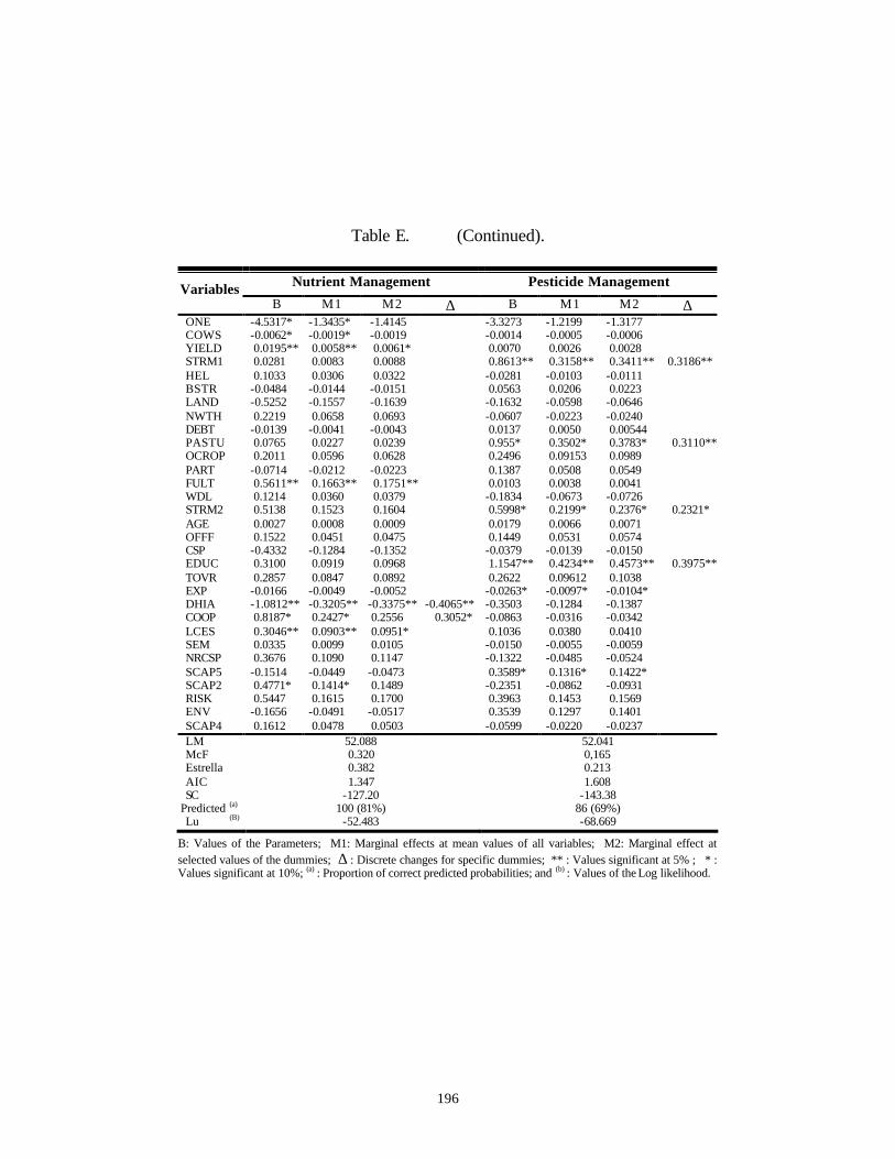
196
Table E. (Continued).
Nutrient Management Pesticide Management Variables B M1 M2 ∆ B M1 M2 ∆
ONE -4.5317* -1.3435* -1.4145 -3.3273 -1.2199 -1.3177 COWS -0.0062* -0.0019* -0.0019 -0.0014 -0.0005 -0.0006 YIELD 0.0195** 0.0058** 0.0061* 0.0070 0.0026 0.0028 STRM1 0.0281 0.0083 0.0088 0.8613** 0.3158** 0.3411** 0.3186** HEL 0.1033 0.0306 0.0322 -0.0281 -0.0103 -0.0111 BSTR -0.0484 -0.0144 -0.0151 0.0563 0.0206 0.0223 LAND -0.5252 -0.1557 -0.1639 -0.1632 -0.0598 -0.0646 NWTH 0.2219 0.0658 0.0693 -0.0607 -0.0223 -0.0240 DEBT -0.0139 -0.0041 -0.0043 0.0137 0.0050 0.00544 PASTU 0.0765 0.0227 0.0239 0.955* 0.3502* 0.3783* 0.3110** OCROP 0.2011 0.0596 0.0628 0.2496 0.09153 0.0989 PART -0.0714 -0.0212 -0.0223 0.1387 0.0508 0.0549 FULT 0.5611** 0.1663** 0.1751** 0.0103 0.0038 0.0041 WDL 0.1214 0.0360 0.0379 -0.1834 -0.0673 -0.0726 STRM2 0.5138 0.1523 0.1604 0.5998* 0.2199* 0.2376* 0.2321* AGE 0.0027 0.0008 0.0009 0.0179 0.0066 0.0071 OFFF 0.1522 0.0451 0.0475 0.1449 0.0531 0.0574 CSP -0.4332 -0.1284 -0.1352 -0.0379 -0.0139 -0.0150 EDUC 0.3100 0.0919 0.0968 1.1547** 0.4234** 0.4573** 0.3975** TOVR 0.2857 0.0847 0.0892 0.2622 0.09612 0.1038 EXP -0.0166 -0.0049 -0.0052 -0.0263* -0.0097* -0.0104* DHIA -1.0812** -0.3205** -0.3375** -0.4065** -0.3503 -0.1284 -0.1387 COOP 0.8187* 0.2427* 0.2556 0.3052* -0.0863 -0.0316 -0.0342 LCES 0.3046** 0.0903** 0.0951* 0.1036 0.0380 0.0410 SEM 0.0335 0.0099 0.0105 -0.0150 -0.0055 -0.0059 NRCSP 0.3676 0.1090 0.1147 -0.1322 -0.0485 -0.0524 SCAP5 -0.1514 -0.0449 -0.0473 0.3589* 0.1316* 0.1422* SCAP2 0.4771* 0.1414* 0.1489 -0.2351 -0.0862 -0.0931 RISK 0.5447 0.1615 0.1700 0.3963 0.1453 0.1569 ENV -0.1656 -0.0491 -0.0517 0.3539 0.1297 0.1401 SCAP4 0.1612 0.0478 0.0503 -0.0599 -0.0220 -0.0237 LM 52.088 52.041 McF 0.320 0,165 Estrella 0.382 0.213 AIC 1.347 1.608 SC -127.20 -143.38
Predicted (a) 100 (81%) 86 (69%) Lu (B) -52.483 -68.669
B: Values of the Parameters; M1: Marginal effects at mean values of all variables; M2: Marginal effect at selected values of the dummies; ∆ : Discrete changes for specific dummies; ** : Values significant at 5% ; * : Values significant at 10%; (a) : Proportion of correct predicted probabilities; and (b) : Values of the Log likelihood.
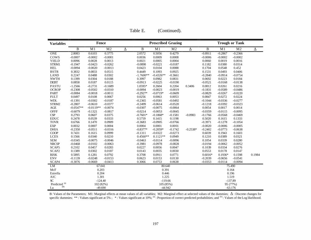
197
Table E. (Continued).
Variables Fence Prescribed Grazing Trough or Tank
B M1 M2 ∆ B M1 M2 ∆ B M1 M2 ∆ ONE 2.8083 0.6103 0.3775 2.0572 0.5056 0.4279 -0.8911 -0.2867 -0.2366 COWS -0.0007 -0.0002 -0.0001 0.0036 0.0009 0.0008 -0.0006 -0.0002 -0.0002 YIELD 0.0096 0.0028 0.0013 0.0021 0.0005 0.0004 0.0060 0.0019 0.0016 STRM1 -0.1947 -0.0423 -0.0262 -0.0898 -0.0221 -0.0187 0.1182 0.0380 0.0314 HEL -0.0094 -0.0020 -0.0013 0.0423 0.0104 0.0088 0.1704 0.0548 0.452 BSTR 0.3832 0.0833 0.0515 0.4449 0.1093 0.0925 0.1531 0.0493 0.0406 LAND 0.2247 0.0488 0.0302 -1.7600** -0.4326** -0.3661 -0.2840 -0.0914 -0.0754 NWTH 0.1399 0.0304 0.0188 0.3997 0.0982 0.0831 0.0692 0.0223 0.0184 DEBT 0.0858 0.0187 0.0115 -0.0913 -0.0225 -0.0190 -0.0521 -0.0168 -0.0138 PASTU -1.2566 -0.2731 -0.1689 1.0595* 0.2604 0.2204 0.3406 0.0812 0.0261 0.0216 OCROP -0.2308 -0.0502 -0.0310 -0.0094 -0.0023 -0.0019 -0.1831 -0.0589 -0.0486 PART -0.0084 -0.0018 -0.0011 -0.2927* -0.0719* -0.0609 -0.0829 -0.0267 -0.0220 FULT 0.0497 0.0108 0.0067 0.0256 0.0063 0.0053 0.0847 0.0272 0.0224 WDL -0.1391 -0.0302 -0.0187 -0.2365 -0.0581 -0.0492 -0.1044 -0.0336 -0.0277 STRM2 -0.2807 -0.0610 -0.0377 -0.2499 -0.0614 -0.0520 -0.1218 -0.0392 -0.0323 AGE -0.0547** -0.0119** -0.0074 -0.0307 -0.0075 -0.0064 0.0054 0.0017 0.0014 OFFF -0.6079 -0.1321 -0.0817 -0.0214 -0.0053 -0.0045 -0.0359 -0.0115 -0.0095 CSP 0.2793 0.0607 0.0375 -0.7601* -0.1868* -0.1581 -0.0983 -0.1766 -0.0568 -0.0469 EDUC 0.2478 0.0539 0.0333 0.5759 0.1415 0.1198 0.5020 0.1615 0.1333 TOVR 0.6766 0.1470 0.0909 -0.3683 -0.0905 -0.0766 -0.3971 -0.1278 -0.1054 EXP 0.0032 0.0007 0.0004 0.0004 0.0001 0.0001 -0.0020 -0.0006 -0.0005 DHIA -0.2350 -0.0511 -0.0316 -0.8377* -0.2059* -0.1742 -0.2538* -0.2402 -0.0773 -0.0638 COOP 0.7431 0.1615 0.0999 -0.1311 -0.0322 -0.0273 0.6039 0.1943 0.1603 LCES 0.1566 0.0340 0.0210 0.4560** 0.1121** 0.0949 0.1210 0.0389 0.0321 SEM -0.0345 -0.0075 -0.0046 -0.0463 -0.0114 -0.0096 0.1054 0.0339 0.0280 NRCSP -0.0468 -0.0102 -0.0063 -0.3981 -0.0978 -0.0828 -0.0194 -0.0062 -0.0052 SCAP5 0.2102 0.0457 0.0283 0.0227 0.0056 0.0047 0.1039 0.0334 0.0276 SCAP2 0.1389 0.0302 0.0187 0.0143 0.0035 0.0030 0.0553 0.0178 0.0147 RISK 0.5895 0.1281 0.0792 0.3708 0.0911 0.0771 0.6016* 0.1936* 0.1598 0.1984 ENV -0.1139 -0.0248 -0.0153 0.0623 0.0153 0.0130 -0.2039 -0.0656 -0.0541 SCAP4 -0.3076 -0.0669 -0.0413 0.3066 0.0753 0.0638 -0.0353 -0.0114 -0.0094 LM 67.041 80.640 75.490 McF 0.203 0.391 0.164 Estrella 0.204 0.446 0.196 AIC 1.301 1.225 1.519 SC -124.40 -119.66 -137.89 Predicted (a) 102 (82%) 105 (85%) 95 (77%) Lu (B) -49.690 -44.942 -63.176
B: Values of the Parameters; M1: Marginal effects at mean values of all variables; M2: Marginal effect at selected values of the dummies; ∆ : Discrete changes for specific dummies; ** : Values significant at 5% ; * : Values significant at 10%; (a) : Proportion of correct predicted probabilities; and (b) : Values of the Log likelihood.
198
VITA
Noro C. Rahelizatovo was born in Antananarivo, Madagascar. Upon completion of a
high school degree at Lycee Jules Ferry, Antananarivo, in 1977, she performed the mandatory
“national” service. She completed her undergraduate degree in 1982, and graduated as an
agricultural engineer, specialized in Food Industry, from the University of Madagascar in 1984.
She has worked at the Service of project Monitoring and Evaluation, Department of
Programming, Ministry of Agriculture, since 1985. She has been responsible of the Division of
Methodology, Coordination and Synthesis. She completed two years of professional training at
the Institute of Madagascar for Techniques of Planning to enhance her professional abilities, and
graduated as a Planner in 1990. In 1993, she was responsible of the Service of Programming,
Department of Programs and Finance, Ministry of Agriculture.
In 1995, she pursued her graduate studies in the Department of Agricultural Economics
and Agribusiness at Louisiana State University, and received her Master of Science degree in
1997. She went back to Madagascar and worked at the Ministry of Agriculture.
She reentered LSU in 1999, to pursue her doctoral program in the Department of
Agricultural Economics and Agribusiness. She received the outstanding doctoral student award
in October 2002. Noro C. Rahelizatovo is now a candidate for the degree of Doctor of
Philosophy in agricultural economics.