Beyond Highway Dimension:Small Distance Labels Using Tree Skeletons∗

Adrian Kosowski and Laurent Viennot

Inria Paris and IRIF, Universite Paris Diderot, France

Abstract

The goal of a hub-based distance labeling scheme for a network G = (V,E) is to assign a smallsubset S(u) ⊆ V to each node u ∈ V , in such a way that for any pair of nodes u, v, the intersectionof hub sets S(u) ∩ S(v) contains a node on the shortest uv-path.

The existence of small hub sets, and consequently efficient shortest path processing algorithms,for road networks is an empirical observation. A theoretical explanation for this phenomenon wasproposed by Abraham et al. (SODA 2010) through a network parameter they called highway dimen-sion, which captures the size of a hitting set for a collection of shortest paths of length at least rintersecting a given ball of radius 2r. In this work, we revisit this explanation, introducing a moretractable (and directly comparable) parameter based solely on the structure of shortest-path spanningtrees, which we call skeleton dimension. We show that skeleton dimension admits an intuitive defi-nition for both directed and undirected graphs, provides a way of computing labels more efficientlythan by using highway dimension, and leads to comparable or stronger theoretical bounds on hubset size.

Key Words: Distance Labeling, Highway Dimension, Shortest Path Tree, Skeleton Dimension

1 Introduction

The task of efficiently processing shortest path queries to a graph has been studied in a plethora of set-tings. One interesting observation is that for many real-world graphs of small degree in a geometric orgeographical setting, such as road networks, it is possible to design compact data structures and schemesfor efficiently answering shortest path queries. The general principle of operation of this approach con-sists in detecting and storing subsets of so-called transit nodes, which appear on shortest paths betweenmany node pairs.

In an attempt to explain the efficiency of variants of the transit node routing (TNR) algorithm [13,14],Abraham et al. [7] introduced the concept of highway dimension h. This parameter captures the intuitionthat when a map is partitioned into regions, all significantly long shortest paths out of each region canbe hit by a small number of transit node vertices. The value of h is presumed to be a small constant e.g.for road networks. However, the definition of highway dimension relies on the notion of a hitting set ofshortest path sets within network neighborhoods, and hence, e.g., exact computation of the parameter isknown to be NP-hard even for unweighted networks [20]. This motivates us to look at other measures,which are both more locally defined and computationally tractable, while capturing essentially the same(or more) characteristics of the network’s amenability to shortest path queries.∗Supported by Inria project GANG, ANR project DESCARTES, and NCN grant 2015/17/B/ST6/01897.

1

arX

iv:1

609.

0051

2v2

[cs

.DS]

12

Dec

201

6

Looking more precisely at the TNR algorithm, one observes that it is built around the idea that forevery source node, the set of transit nodes which are the first to be encountered when going a longway from the source, is small. This is a weaker assumption than the existence of a small hitting setfor the set of shortest paths in a given network neighborhood, since different source nodes could usedifferent transit nodes resulting in an overall large number of transit nodes around a given region. Thissource-centered approach leads us to the definition of skeleton dimension k , to which we devote theremainder of this paper. Informally, the skeleton dimension is the maximum, taken over all nodes uof the graph and all radii r > 0, of the number of distinct nodes at distance r from u in the set of allshortest paths originating at u and having length at least 3r/2.1 In transit node parlance, it states that thepaths from u that extend by r/2 at least outside the disk of radius r pass through at most k transit nodesat the disk border. This property ensures that each shortest-path spanning tree is built around a coreskeleton with at most k branches at a given distance range while the rest of the branches are relativelyshort. Bounding tree skeletons turns out to encompass a larger class of constant-degree graphs thanthe shortest path cover approach used in the definition of highway dimension, while still ensuring theexistence of efficient labeling schemes.

Motivated by applications in distributed algorithms and distributed data representation, we will dis-play the link between small skeleton dimension of a graph and efficient processing of shortest pathqueries using the framework of distance labeling. Distance labeling schemes, popularized by Gavoilleet al. [21], are among the most fundamental distributed data structures for graph data. Within distancelabeling, we work with the most basic framework of transit-node based schemes, namely so-called hublabelings, cf. [5] (this framework was first described in [18] under the name of 2-hop covers, and is alsoreferred to as landmark labelings [8]). In this setting, each node u ∈ U stores the set of its distances tosome subset S(u) ⊆ V of other nodes of the graph. Then, the computed distance value d′(u, v) for aqueried pair of nodes u, v ∈ V is returned as:

d′(u, v) := minw∈S(u)∩S(v)

d(u,w) + d(w, v), (1)

where d denotes the shortest path distance function between a pair of nodes. The computed distancebetween all pairs of nodes u and v is exact if set S(u)∩S(v) contains at least one node on some shortestu − v path. This property of the family of sets (S(u) : u ∈ V ) is known as shortest path cover.The hub-based method of distance computation is in practice effective for two reasons. First of all, fortransportation-type networks it is possible to show bounds on the sizes of sets S, which follow from thenetwork structure. Notably, considering networks of bounded highway dimension h, Abraham et al. [7]show that an appropriate cover of all shortest paths in the graph can be achieved using sets S of sizeO(h), where the O-notation conceals logarithmic factors in the studied graph parameters.

Moreover, the order in which elements of sets S(u) and S(v) is browsed when performing the min-imum operation is relevant, and in some schemes, the operation can be interrupted once it is certain thatthe minimum has been found, before probing all elements of the set. This is the principle of numerousheuristics for the exact shortest-path problem, such as contraction hierarchies and algorithms with arcflags [15, 25].

1.1 Results and Organization of the Paper

In Section 2, we formally define skeleton dimension k , and show that in the so-called continuous repre-sentation of the graph, the skeleton dimension is at most highway dimension, i.e. it satisfies the boundk ≤ h. In all cases, k = O(h) for graphs of bounded maximum degree. On the other hand, we show that

1One may also define skeleton dimension with a different choice of constants, considering the set of shortest paths havinglength at least αr, where α ∈ (1, 2) is an absolute constant. The choice of α = 3/2 is subsequently necessary only forestablishing relations with highway dimension.

2

skeleton dimension provides a better explanation for small hub set size in Manhattan-type networks thanhighway dimension. In particular, we provide a natural example of a weighted grid with k = O(log n)and h = Ω(

√n).

In Section 3, we show how to construct efficient hub labelings for networks of small skeleton dimen-sion. The hub set sizes we obtain for a graph of weighted diameter D are bounded by O(k logD) onaverage and O(k log log k logD) in the worst case (cf. Corollaries 1 and 3, respectively), as comparedto previous best bounds ofO(h log h logD) for labels computable in polynomial time based on highwaydimension.

Our labeling technique, based on picking hubs through a random selection process on a subtree ofthe shortest-path tree, allows each node to compute its hub set independently in almost-linear time, andappears to be of independent interest. In particular, as an extension of our technique, we provide inSection 4 improved bounds on label size (in general unweighted graphs) for the so-called δ-preservingdistance labeling problem, in which the considered distance queries are restricted to nodes at distance atleast δ from each other. The hub sets constructed using the hub-based method have average sizeO(n/δ).Their worst-case size is also bounded by O(n/δ) up to some threshold δ = O(

√n), and bounded by

O(log δ+ (n/δ) log log δ) in general (Theorem 2). This improves upon previous δ-preserving schemes,including the previously best result from [10], where hub sets of worst-case size O((n/δ) log δ) areconstructed by a more direct application of the probabilistic method to sets of randomly sampled vertices.

Finally, in Sections 5, 6, and 7 we provide some concluding remarks on the computability of theproposed parameter of skeleton dimension, as well as its possible generalizations and applications.

1.2 Other Related Work

Distance Labelings. The distance labeling problem in undirected graphs was first investigated byGraham and Pollak [23], who provided the first labeling scheme with labels of size O(n). The decodingtime for labels of size O(n) was subsequently improved to O(log log n) by Gavoille et al. [21] and toO(log∗ n) by Weimann and Peleg [29]. Finally, Alstrup et al. [11] present a scheme for general graphswith decoding in O(1) time using labels of size log 3

2 n + o(n) bits. This matches up to low order termsthe space of the currently best know distance oracle with O(1) time and log 3

2 n2 + o(n2) total space in acentralized memory model, due to Nitto and Venturini [27]. For specific classes of graphs, Gavoille etal. [21] described aO(

√n log n) distance labeling for planar graphs, together with Ω(n1/3) lower bound

for the same class of graphs. Additionally, O(log2 n) upper bound for trees and Ω(√n) lower bound for

sparse graphs were given.

Distance Labeling with Hub Sets. For a given graph G, the computational task of minimizing thesizes of hub sets (S(u) : u ∈ V ) for exact distance decoding is relatively well understood. A O(log n)-approximation algorithm for minimizing the average size of a hub set having the sought shortest pathcover property was presented in Cohen et al. [18], whereas a O(log n)-approximation for minimizingthe largest hub set at a node was given more recently in Babenko et al. [12]. Rather surprisingly, thestructural question of obtaining bounds on the size of such hub sets for specific graph classes, such asgraphs of bounded degree or unweighted planar graphs, is wide open.

δ-preserving Labeling. The notion of δ-preserving distance labeling, first introduced by Bollobas etal. [16], describes a labeling scheme correctly encoding every distance that is at least δ. [16] presentssuch a δ-preserving scheme of size O(nδ log2 n). This was recently improved by Alstrup et al. [10] toa δ-preserving scheme of size O(nδ log2 δ). Together with an observation that all distances smaller thanδ can be stored directly, this results in a labeling scheme of size O(nx log2 x), where x = logn

log m+nn

. For

sparse graphs, this is o(n).

3

Road networks. Highway dimension h guarantees the existence of distance labels of size O(h logD)where D is the weighted diameter of the graph [7]. However, when restricting to polynomial timealgorithms, such labels can only be approximated within a log n factor using shortest path cover algo-rithms [7] or a log h factor with a more involved procedure based on VC-dimension [3]. In any case, thisrequires an all-pair shortest path computation. For large networks, labels can be practically computedwhen classical heuristics such as contraction hierarchies (CH) can be performed [4, 6, 7]. Low highwaydimension guarantees that there exists an elimination ordering for CH such that the graph produced hasbounded size [7]. However, it does not ensure running time faster than all pair shortest path computation.

Besides highway dimension, skeleton dimension is also related to the notion of reach introducedin [24] and also used in the RE algorithm [22]. The reach of a node v on a pathP is the minimum distanceto an extremity of P , and the reach of v is its maximum reach over all shortest paths P containing v.Efficient algorithms are obtained by pruning nodes with small reach during Dijkstra search. Similarly,we obtain the skeleton of a tree by pruning nodes whose reach (in the tree) is less than half of theirdistance to the root.

1.3 Notation and Parameters

We consider a connected undirected graph G and a non-negative length function ` : E(G)→ R+. Let ndenote the number of nodes in V (G). We let `(P ) denote the length of a path P under the given lengthfunction. Given two nodes u and v, we assume that there is a unique shortest path Puv between them.This common assumption can be made without loss of generality, as one can perturb the input to ensureuniqueness. Given two nodes u and v, their distance is dG(u, v) = `(Puv). Let D = maxu,v dG(u, v)denote the diameter of G. For u ∈ V (G) and r > 0, the ball BG(u, r) of radius r centered at u isthe set of nodes v with dG(u, v) ≤ r. In this paper, we assume that ` is non-negative and integral. Thenotions presented here easily extend to non-negative real lengths, but we use integer lengths for a cleanerexposition of algorithms and theorems.

We also recall two structural parameters, which have application to networks in a geometric settingor low-dimensional topological embedding: highway dimension and doubling dimension.

For r > 0, let PG(r) denote the collection of all shortest paths P with r2 < `(P ) ≤ r in G. For

u ∈ V (G), we consider the collection PG(u, r) = P ∈ Pr(G) | P ∩BG(u, r) 6= ∅ of shortest pathsaround u. A hitting set for PG(u, r) is a set H of nodes such that any path in PG(u, r) contains a nodein H . In [3], the highway dimension of G is defined as the smallest h such that PG(u, r) has a hitting setof size at most h for all u, r. (This definition is slightly less restrictive than that of [7] while allowing toprove similar results with improved bounds.)

The notion of highway dimension is related to that of doubling dimension. Recall that a graph ish-doubling if any ball can be covered by at most h balls of half the radius. That is, for all u, r, thereexists H with |H| ≤ h such that BG(u, r) ⊆ ∪v∈HBG(v, r2). It is shown in [7] that if the geometricrealization of a graph G has highway dimension h, then G is h-doubling. Informally, the geometricrealization G can be seen as the “continuous” graph where each edge is seen as infinitely many verticesof degree two with infinitely small edges, such that for any uv ∈ E(G) and t ∈ [0, 1], there is a node inG at distance t`(u, v) from u on edge uv. (The proof in [7] consists in proving that any node inBG(u, r)is at distance at most r2 from any hitting set of P

G(u, r) in G and holds also for the highway dimension

definition of [3].)

2 A Presentation of Skeleton Dimension

We start by providing a standalone definition of skeleton dimension based on size of cuts in shortestpath trees, and then show its relation to the previously considered parameters of highway and doublingdimension.

4

2.1 Definition of the Parameter

Tree skeleton. Given a tree T rooted at node u with length function ` : E(T ) → R+, we treat it asdirected from root to leaves and consider the geometric realization T of this directed graph. We definethe reach of v ∈ V (T ) as Reach

T(v) := max

x∈V (T )dT

(v, x). We then define the skeleton T ∗ of T as

the subtree of T induced by nodes with reach at least half their distance from the root. More precisely,T ∗ is the subtree of T induced by v ∈ V (T ) | Reach

T(v) ≥ 1

2dT (u, v).

Width of a tree. The width of a tree T with root u is defined as the maximum number of nodes (points)in T at a given distance from its root. More precisely, the width of T is Width(T ) = maxr>0 |Cutr(T )|where Cutr(T ) is the set of nodes v ∈ V (T ) with d

T(u, v) = r.

Skeleton dimension. The skeleton dimension k of a graph G is defined as the maximum width of theskeleton of a shortest path tree, that is k = maxu∈V (G) Width(T ∗u ), where Tu denotes the shortest pathtree of u obtained as the union of shortest paths from u to all v ∈ V (G).

We remark that, under the assumption of scale-invariance of the graph, different cuts of the treeskeleton have similar width, and the definition of the skeleton dimension is a meaningful measure of thestructure of the tree. A smoothed (integrated) variant of skeleton dimension is also discussed further on,cf. Eq. (2).

2.2 Skeleton Dimension is at most (Geometric) Highway Dimension

Claim 1. If the geometric realization G of a graph G has highway dimension h, then G has skeletondimension k ≤ h.

Proof. Consider a node u and the skeleton T ∗u of its shortest path tree Tu. For r > 0, consider thecut Cutr(T ∗u ). For ε > 0 sufficiently small, Cutr(T ∗u ) and Cutr−ε(T

∗u ) have same size. Now, for

v ∈ Cutr−ε(T∗u ), consider a node x in Tu such that dTu(v, x) = ReachTu(v). The shortest path Pvx

intersectsBG(u, r) and has length `(Pvx) = ReachTu(v) ≥ r/2+ε > r/2. Pvw is thus in PG

(u, r). Foreach node in Cutr−ε(T

∗u ), we get a similar path in P

G(u, r). All these paths are pairwise node-disjoint

as they belong to disjoint sub-branches of Tu. Their number is thus upper-bounded by the size of anyhitting set of P

G(u, r). We then get |Cutr(T ∗u )| ≤ h for all u, r and the skeleton dimension of G is at

most h.

Note that a (discrete) graph G has highway dimension h ≤ h, where h is the highway dimension ofits geometric realization G. In road networks it is expected that the continuous and the discrete versionsof highway dimension coincide almost exactly, in particular due to the constant maximum degree andbounded length of edges in these graphs. In a more general setting, one can easily show h ≤ (∆ + 1)hwhere ∆ is the maximum degree of G, with a star being a worst-case example. (Indeed, a hitting set Hof PG(u, r) may miss some shortest path P ∈ P

G(u, r). Making P longer to have extremities in V (G)

transforms it into a path of PG(u, r) that is hit by H . It is thus possible to hit all PG

(u, r) by adding atmost one node per edge adjacent to a node in H .)

We remark that the extended tech-report version [2] of [7] introduces a modified notion of highwaydimension, in a way more closely related to its geometric variant, which we can denote here as h∗. Forthis modified parameter, we have: k ≤ h∗ ≤ h ≤ 2h∗, where the first inequality follows from ananalysis similar to the proof of Claim 1, while the latter two are shown in [2][Section 11].

5

2.3 Low Skeleton Dimension Implies Low Doubling Dimension

It is known [7] that a graph having a geometric realization with highway dimension h is at most h-doubling. However, the relation k ≤ h need not be tight, and it turns out that the link between skeletondimension and doubling dimension holds in a slightly weaker form.

Proposition 1. If a graph G has skeleton dimension k , then G is (2 k +1)-doubling.

Proof. We show the stronger requirement that each ball of radius 19r/9 can be covered by 2 k +1 ballsof radius r. For u ∈ V (G), consider the shortest path tree Tu of u. For r′ > 0, consider the set Cr′ ofthe edges containing a node in Cutr′(T

∗u ) and let Ir′ = w | vw ∈ Cr′ and dG(u,w) ≥ r′ be the (at

most k ) far extremities of edges cutting distance r′ in the skeleton of Tu. Each node v at distance greaterthan 3

2r′ from u is descendant in Tu of a node x ∈ Ir′ by skeleton definition and is thus in BG(x, r) if

dG(u, v) ≤ r′ + r. Considering r′ = 2r/3, we obtain that any node v with r < dG(u, v) ≤ 53r is at

distance at most r from a node in I2r/3. Similarly any node v with 53r < dG(u, v) ≤ 19

9 r is at distanceat most r from a node in I10r/9. The ball BG(u, 19r/9) is thus covered by balls of radius r centered atthe at most 2 k +1 nodes in u ∪ I2r/3 ∪ I10r/9.

2.4 Separating Skeleton Dimension and Highway Dimension

We now provide a family of graphs which exhibit an exponential gap between skeleton and highwaydimensions, in a setting directly inspired by Manhattan-type road networks. The idea is to considerthe usual square grid and define edge lengths, which give priority to certain transit “arteries”. In ourexample, paths using edges whose coordinates are multiples of high powers of 2 have slightly lowertransit times.

For L > 0, let GL denote the 2L × 2L grid with length function ` defined as follows. We iden-tify a node with its coordinates (x, y) with 1 ≤ x ≤ 2L and 1 ≤ y ≤ 2L. We consider smalllength perturbations pxy for every horizontal edge (x, y), (x + 1, y) and qxy for every vertical edge(x, y), (x, y + 1), and define Q = 1 + maxx,y maxpxy, qxy. These non-negative integers will bechosen to ensure uniqueness of shortest paths. For x = 2ix′ with 0 ≤ i ≤ L and x′ odd, we define`((x, y), (x+ 1, y)) = Q((D+ 2)L− i)− qxy for all y where D = 2L+3. For y = 2jy′ with 0 ≤ j ≤ Land y′ odd, we define `((x, y), (x, y + 1)) = Q((D + 2)L − j) − pxy for all x. A possible choice forperturbations ensuring uniqueness of shortest paths is pxy = 0 and qxy = x for all x, y as will be clearlater on.

Proposition 2. For any L > 0, grid GL has highway dimension Ω(√n) and skeleton dimension

O(log n), where n = 22L is the number of nodes in GL.

Proof. We first prove that the shortest paths of GL are also shortest path of the 2L × 2L grid UL withunit edge lengths, that is those paths that use a minimum number of edges. Any path P with p edges haslength at most pQ(D+ 2)L and at least pQ((D+ 2)L−L−1) ≥ pQDL. Given two nodes u and v, letp denote the minimum number of edges of a path from u to v and let q denote the number of edges of theshortest path Puv from u to v in GL. We then have p ≤ q ≤ p(D+2)L

DL ≤ p+ 12 since p ≤ 2L+1 = D/4.

This implies q = p. Puv is thus a shortest path of the grid UL. Note that balls must then also be almostidentical: for all u, p, we have BGL(u, pQ(D + 2)L) = BUL(u, p).

This implies that the highway dimension ofGL is Ω(√n) since the ball of radius r = Q(D+2)L

√n

centered at (1, 1) intersects at least√n horizontal shortest paths of length QDL

√n > r/2 at least.

We define the 2i × 2j rectangle R at (x, y) with odd x and y as the set of nodes with coordinates(x′, y′) such that 2ix ≤ x′ ≤ 2i(x+1) and 2jy ≤ y′ ≤ 2j(y+1). Its border is the set of nodes for whichone inequality at least is indeed an equality. Other nodes are said to be interior. The main argument forbounding skeleton dimension is that a shortest path from u = (x′, y′) with x′ < 2ix and y′ < 2jy cannot

6

traverse the interior of R: a shortest path passing through an inner node of R necessarily ends insideR. The reason is that such a path necessarily passes through the lower left corner at (2ix, 2jy). It isthen shorter to reach a border node by following the border rather than using edges inside the rectangle.Note that two possible choices of shortest paths could be possible when going from a corner of a 2i× 2i

rectangle to the corner diagonally opposed. However the choice of perturbing lengths by decreasing thelength of any vertical edge in position (x, y) by qxy = x ensures that the path through the rightmost sideis preferred.

Now consider a node u = (x, y) and a radius r with 2iQDL ≤ r < 2i+1QDL. Set p =⌊

rQDL

⌋.

According to the first part of the proof, the ball BGL(u, r) is in sandwich between the balls of radius pand p+ 1 in UL: BUL(u, p) ⊆ BGL(u, r) ⊆ BUL(u, p+ 1). We first consider the upper right quadrantof BUL(u, p) and the border set SUR of nodes v = (x+ a, y + b) with a, b ≥ 0 and a+ b = p. We nowbound the number of nodes v ∈ SUR such that ReachTu(v) > r

2 where Tu denote the shortest path treeof u in GL. As r

2 ≥ 2i−1QDL, such a node v cannot be interior to a 2i−2 × 2i−2 rectangle as shortestpaths interior to the rectangle have length at most (2i−1 − 4)Q(D + 2)L. The number of nodes in SURwhose x coordinate is a multiple of 2i−2 is bounded by 8 as p < 2i+1. Similarly, the number of nodeswhose y coordinate is a multiple of 2i−2 is also bounded by 8. Apart from these 16 nodes, we have toconsider nodes v = (x′, y′) where x′ (resp. y′) is less than the smallest multiple of 2i−2 greater thanx (resp. y). Such a node cannot be interior to a 2j × 2i−2 (resp. 2i−2 × 2j) rectangle for j ≤ i − 3.For j = i − 3, we obtain at most two nodes whose x coordinate is a multiple of 2j . By repeating theargument for j = i − 4..1, we can finally bound the number of nodes v ∈ SUR with reach greater thanr/2 by 4(i− 3) + 16 = 4(i+ 1). Nodes in the upper right quadrant that are at distance r from u in Tumust be on edges outgoing from nodes in SUR and Cutr(T

∗u ) has thus size at most 8(i+ 1) = O(log n).

By symmetry, the bound holds for other quadrants and the skeleton dimension of GL is O(log n).

We remark that there exist different lengths functions on the grid for which the skeleton dimensionis also as large as Θ(

√n). This is the case, for example, for a grid with unit lengths of all edges except

for edges intersecting its major diagonal, which is configured to be a fast transit artery (it suffices to set`((x, y), (x+ 1, y)) = 0.5 for all x = y).

We complement this result with experimental observation in real grid like networks such as encoun-tered in Brooklyn. We computed the skeleton dimension of the New York travel-time graph proposed inthe 9th DIMACS challenge [1] which turns out to be k = 73. (Average skeleton tree width is 30, but amaximum width of 73 is encountered for a skeleton tree rooted in Manhattan.) In order to estimate thehighway dimension of this graph, we have implemented a heuristic for finding a large packing of pathsnear a given ball, that is a set of disjoint paths intersecting the ball and having length greater than halfradius. We could find a packing of 172 paths in Brooklyn. This proves that the highway dimension ofthis graph is 172 at least (h ≥ 172). In comparison the skeleton tree of the center of the correspondingball has width 48, and 42 branches are cut at radius distance (see Figure 1).

3 Hub Labeling using Tree Skeletons

In this section, we assign shortest-path-intersecting hub sets to a set of (terminal) nodes V of the con-sidered network. We will assume that the length function ` on edges is integer weighted. To emulatethe geometric realization of the graph, we subdivide edges into sufficiently short fragments by insertinga set of additional nodes V + into the network. For convenience of subsequent analysis, we assume thatan edge vw, for v, w ∈ V , of integer length `(vw) is subdivided into 12`(vw) edges of length 1/12each. After this, all edges have the same length, and we subsequently treat the graph as unweighted. Allthe parameter definitions carry over directly from the geometric setting; for the sake of precision, weformally state the assumptions on the studied setting below.

7

Figure 1: An OpenStreetMap view of Brooklyn, with a packing of 172 paths (in black) intersecting aball of radius 720 seconds (with white border) on the left, and the skeleton tree (in black) of the centerof the ball on the right.

We consider an unweighted graph G = (V ∪ V +, E), with a distinguished set of terminal nodes Vand where all nodes from V + have degree 2. We denote n := |V |. We assume that every node u ∈ V isassociated with a fixed (unweighted) tree Tu ⊆ G. Throughout the section, we will denote by Pu(v, w)the unique path between the pair of nodes v and w in tree Tu, and more concisely Pu(v) := Pu(u, v).Where this does not lead to confusion, we will identify a path with its edge set, and we will also usethe symbol |P | to denote the length of path P , i.e., the number of edges belonging to P . We writedu(v) := |Pu(v)|. We require that the collection of trees Tuu∈V satisfies the following property: Forany pair of nodes u, v ∈ V , we have Pu(v) = Pv(u). We will also assume that for all u, v, w ∈ V , wehave that |Pu(v, w)| is an integer multiple of 12.

We remark that if the graph G was obtained by a distance-preserving subdivision of nodes of anedge-weighted graph on node set V under some distance metric `, then each tree Tu ∈ G corresponds tothe shortest path tree of node u under the original distance metric, and the assumption Pu(v) = Pv(u)corresponds to the assumption of uniqueness of shortest paths under the original metric `.

An edge hub labeling is an assignment of a set of edges S(u) ⊆ E to each node u ∈ V , such that thefollowing property is fulfilled: for every pair of nodes u, v ∈ V , there exists an edge η ∈ S(u) ∩ S(v)such that η ∈ Pu(v). The set S(u) is known as the edge hub set of u. We remark that this edge-basednotion of hub sets is slightly stronger than an analogous vertex-based notion: indeed, knowing that anedge η ∈ Pu(v), we also conclude that both of the endpoints of edge η belong to Pu(v). We choose towork with edge hub sets rather than node hub sets in this Section for compactness of arguments.

We restate in the setting of the family of trees Tuu∈V the notion of the skeleton T ∗u = Tu[V ∗u ] ⊆ Tuas the subtree of Tu induced by node set V ∗u = v ∈ V (Tu) : ReachTu(v) ≥ 1

2du(v). For u ∈ V , the

width Width(T ∗u ) of the skeleton T ∗u may be written as Width(T ∗u ) = maxr∈N |Cut∗(r)u |, where:

Cut∗(r)u := v ∈ V ∗u : du(v) = r.

Finally, we note that the skeleton dimension of graph G may be written as k = maxu∈V Width(T ∗u ).

8

3.1 Construction of the Hub Sets

The edge hub sets S(u), u ∈ V , are obtained by the following randomized construction. Assign toeach edge e ∈ E a real value ρ(e) ∈ [0, 1], uniformly and independently at random. We condition allsubsequent considerations on the event that all values ρ are distinct, |ρ(E)| = |E|, which holds withprobability 1.

For all u, v ∈ V , we define the central subpath P ′u(v) ⊆ Pu(v) as the subpath of Pu(v) consistingof its middle du(v)

6 edges; formally, P ′u(v) := Pu(u′, v′), where u′, v′ ∈ Pu(v) are nodes given by:du(u′) = 5

12du(v) and du(v′) = 712du(v). Next, for all u, v ∈ V , v 6= u, we define the hub edge

ηu(v) ∈ Pu(v) as the edge with minimum value of ρ on the central subpath between u and v:

ηu(v) = arg mine∈P ′u(v)

ρ(e).

Finally, for each node u ∈ V , we adopt the natural definition of edge hub set S(u) as the set of all edgehubs of node u on paths to all other nodes:

S(u) := ηu(v) : v ∈ V, v 6= u .

Proof of Correctness. Taking into account that for all u, v ∈ V , Pu(v) = Pv(u), we observe thatby symmetry of the central subpath with respect to its two endpoints, we also have P ′u(v) = P ′v(u). Itfollows directly that ηu(v) = ηv(u). Hence, we have ηu(v) ∈ S(u) ∩ S(v), and also ηu(v) ∈ Pu(v),which completes the proof of correctness of the edge hub labeling.

We devote the rest of this Section to bounding the size of hub sets S(u).

3.2 Bounding Average Hub Set Size

In subsequent considerations we will fix a node u ∈ V , and restrict considerations to the tree Tu. Wewill assume that tree Tu is oriented from its root u towards its leaves, and we will call a path P ⊆ Tu adescending path in Tu if one of its endpoints is a descendant of the other in Tu. In particular, every pathPu(v) is a descending path. For an edge e ∈ Tu, we will denote by e+ and e− the two endpoints of e, withe− being the one further away from the root (du(e−) = du(e+) + 1). Likewise, for a descending pathP , we denote by P+ and P− its two extremal vertices, closest and furthest from the root u, respectively.We also denote by du(e) := du(e−) the distance of edge e from the root.

In order to bound the expected size of the hub set S(u), we will observe that elements of S(u) nec-essarily belong to the skeleton T ∗u and satisfy certain minimality constraints with respect to descendingpaths of sufficiently large length, contained entirely within the skeleton T ∗u .

Lemma 1. Let η ∈ S(u), for some u ∈ V . Then, the following claims hold:

(1) η ∈ E(T ∗u ).

(2) ReachT ∗u (η−) ≥ 17du(η).

(3) There exists a descending path P ⊆ T ∗u , such that η = arg mine∈P ρ(e) and |P | ≥ 27du(η).

Furthermore, the following claims hold for any edge η ∈ E satisfying Claims (1) and (3):

(4) There exists a descending path P ⊆ T ∗u , such that η = arg mine∈P ρ(e), η is one of the twoextremal edges of P (i.e., P+ = η+ or P− = η−), and |P | =

⌈17du(η)

⌉.

(5) There exists a descending path Pu(x, y), for some y ∈ V ∗u and x ∈ V ∗u satisfying du(x) =⌊78du(y)

⌋, such that η = arg mine∈Pu(x,y) ρ(e) and η is one of the two extremal edges of Pu(x, y).

9

Proof. Select η ∈ S(u) arbitrarily. Let v ∈ V be any node such that η = ηu(v). We recall that for thedescending path Pu(u′, v′) ⊆ Pu(v), we have η = arg mine∈Pu(u′,v′) ρ(e), where du(u′) = 5

12du(v)

and du(v′) = 712du(v). Let v′′ ∈ Pu(v) be a node such that du(v′′) = 2

3du(v) (we recall that 12|du(v)by assumption). By the definition of skeleton T ∗u , we have v′′ ∈ V ∗u , and clearly Pu(v′′) ⊆ T ∗u . We notethat η ∈ Pu(v′′) and moreover:

ReachT ∗u (η−) ≥ |Pu(η−, v′′)| ≥ |Pu(v′, v′′)| = 2

3du(v)− 7

12du(v) =

1

12du(v) =

1

7du(v′) ≥ 1

7du(η),

hence Claims (1) and (2) follow. To show Claim (3), we put P = Pu(u′, v′) and observe that η =arg mine∈P ρ(e) by definition, and:

|P | = |Pu(u′, v′)| = 7

12du(v)− 5

12du(v) =

1

6du(v) =

2

7du(v′) ≥ 2

7du(η).

Next, to show Claim (4), we observe that by Claim (3), η = arg mine∈Pu(u′,η−) ρ(e) and η = arg mine∈Pu(η+,v′) ρ(e).Moreover, since |Pu(u′, v′)| ≥ 2

7du(η), we have |Pu(u′, η−)|+|Pu(η+, v′)| ≥ 1+27du(η) ≥ 2

⌈17du(η)

⌉,

and so |Pu(u′, η−)| ≥⌈

17du(η)

⌉or |Pu(η+, v′)| ≥

⌈17du(η)

⌉. Claim (4) thus follows for an appropriate

choice of descending path P ⊆ |Pu(u′, η−)| or P ⊆ |Pu(η+, v′)|, respectively, with |P | =⌈

17du(η)

⌉.

Finally, to show Claim (5), we consider separately the two cases from the proof of Claim (4).If P ⊆ Pu(u′, η−), then we set y = η−, and choose x ∈ Pu(η−) so that du(x) = b7

8du(η−)c. Wehave du(x, y) = d1

8du(η−)e ≤ d17du(η−)e = |P |, hence Pu(x, y) ⊆ P , η = arg mine∈Pu(x,y) ρ(e), and

the claim follows.If P ⊆ Pu(η+, v′), then we set x = η+, and choose y ⊆ Pu(x, v′) so that du(x) = b7

8du(y)c. Sucha choice of y is always possible since, when moving with y along the path P , the value of b7

8du(y)cincreases by at most 1 in every step; moreover, for the lower end node v∗ of path P we have du(v∗) >du(x) + 1

7du(x), and so du(x) ≤ b78du(v∗)c. We again obtain η = arg mine∈Pu(x,y) ρ(e), and the claim

follows.

We remark that the remainder of our analysis is valid for any construction of hub sets S whichsatisfies Claims (1), (2), and (3) of Lemma 1.2

To bound the average hub set size precisely, we introduce for each node u a parameter called inte-grated skeleton dimension k(u), defined through a sum of inverse distances to u over nodes of its treeskeleton:

k(u) :=∑v∈V ∗u

1

du(v)=∑r∈N

|Cut∗(r)u |r

, (2)

where the equivalence of the two definitions follows directly from the definition of cuts, Cut∗(r)u = v ∈V ∗(u) : du(v) = r.

Taking into account that |Cut∗(r)u | ≤Width(T ∗u ), we have k(u) = O(Width(T ∗u ) logD(T ∗u )), andeven more roughly, we have for all u ∈ V :

k(u) = O(k logD), (3)

where we recall that D = maxu∈V D(Tu).

2One may, in particular consider an alternative construction of a hub set S+(u), defined as the set of all edges η ∈ E(Tu)which satisfy Claims (1), (2), and (3) of the Lemma. All of our bounds on hub set size also hold in the case of S+(u)u∈V .The definition results in larger labels in practice: we always have S(u) ⊆ S+(u) (correctness results from this observation).On the other hand, hub sets S+(u) may sometimes be constructed more efficiently than S(u): the definition of S(u) requiresa scan of the entire tree T (u), whereas hub set S+(u) may be constructed based only on the smaller skeleton T ∗(u).

10

Lemma 2. The expected hub set size of a node u ∈ V satisfies the bound:

E|S(u)| ≤ 16 k(u).

Proof. Fix u ∈ V arbitrarily. For y ∈ V ∗u , we define xy as the unique node on the path Pu(y) such thatdu(xy) =

⌊78du(y)

⌋. We define random variable Qu(y) ∈ 0, 1 as the number of extreme edges e of

the path Pu(xy, y) (i.e., e+ = xy or e− = y), which satisfy e = arg min ρ(Pu(xy, y)). We have:

Pr[Qu(y) = 1] =2

|Pu(xy, y)|≤ 2

du(y)− 78du(y)

=16

du(y).

By Claim (5) of Lemma 1, it follows that by summing random variables Qu(y) exhaustively over allvertices y we count each element η ∈ S(u) at least once, hence:

|S(u)| ≤∑y∈V ∗u

Qu(y).

By linearity of expectation, it follows that:

E|S(u)| ≤∑y∈V ∗u

EQu(y) =∑y∈V ∗u

Pr[Qu(y) = 1] ≤∑y∈V ∗u

16

du(y).

A direct application of Markov’s inequality to the bound from Lemma 2, combined with Eq. (3),gives the following Corollary.

Corollary 1. The average hub set size satisfies 1n

∑u∈V |S(u)| = O( 1

n

∑u∈V k(u)) ≤ O(k logD),

with probability at least 1/2 w.r.t. choice of random values ρ.

Obtaining concentration bounds on the maximal size of a hub set, maxu∈V |S(u)|, requires somemore care, and we proceed with the analysis in the following subsection.

3.3 Concentration Bounds on Hub Set Size

For fixed u ∈ V , we consider the size of the hub set of u given by the random variable:

|S(u)| =∑

η∈E(T ∗u )

X(η), (4)

where X(η) ∈ 0, 1 is the indicator variable for the event “η ∈ S(u)”. The random variablesX(η)η∈E(T ∗u ) need not, in general, be independent or negatively correlated. In the subsequent analy-sis, for fixed η, we make use of Claim (4) of Lemma 1 to bound random variable X(η). By the Claim ofthe Lemma, we can decompose X(η) into the contributions from descending paths located towards theroot and away from the root with respect to η:

X(η) ≤ X+(η) +X−(η),

where we define:

• X+(η) ∈ 0, 1 is the indicator variable for the event: “for the unique descending subpathP ⊆ Pu(η−) of length |P | =

⌈17du(η)

⌉ending in edge η (i.e., P− = η−), it holds that

η = arg min ρ(P )”,

• X−(η) ∈ 0, 1 is the indicator variable for the event: “there exists a descending path P ⊆ T ∗u oflength |P | =

⌈17du(η)

⌉starting in edge η (i.e., P+ = η+), such that η = arg min ρ(P )”.

11

Moreover, by Claim (2) of Lemma 1, we may have X(η) 6= 0 only for those edges η for whichReachT ∗u (η−) ≥ 1

7du(η). We denote V ∗∗u = v ∈ V ∗u : ReachT ∗u (v) ≥ 17du(v) and T ∗∗u = Tu[V ∗∗u ].

We can now rewrite Eq. (4) as:

|S(u)| ≤∑

η∈E(T ∗∗u )

X+(η) +∑

η∈E(T ∗∗u )

X−(η), (5)

and proceed to bound both of these sums separately. In order to be able to manipulate the sums moreconveniently, we first introduce a partition of the tree according to geometrically increasing scales ofdistance.

Partition of T ∗u into Layers. We consider a sequence of increasing integer radii (r[i])i∈N, given asr[0] = 0 and r[i] =

⌈15(

1615

)i⌉, for i ≥ 1. The last non-empty layer corresponds to index imax <

log16/15 D < 16 lnD . Cutting the edge set of tree T ∗u at vertices located at distances r[i]i∈N from theroot u yields the following partition into layers:

E(T ∗u ) =⋃i∈N

L∗[i], where: L∗[i] := e ∈ E(T ∗u ) : r[i] < du(e) ≤ r[i+1].

We further denote the subset of each layer restricted to edges from T ∗∗u as L∗∗[i] := L∗[i] ∩ E(T ∗∗u ),i ∈ N.

Lemma 3. For all i ≥ 1, edge set L∗∗[i] admits a partition into paths, L∗∗[i] =⋃lij=1 P

[i,j], such that

li < 2 minr∈[r[i+1],r[i+2]] |Cut∗(r)u | ≤ 2 k , each P [i,j] is a descending path, and all internal nodes of all

paths P [i,j] have degree exactly 2 in T ∗∗u .

Proof. Define partition L∗∗[i] =⋃lij=1 P

[i,j] of the edge set of the considered layer so that each pathP [i,j], 1 ≤ j ≤ li, is a maximal descending path whose internal nodes all have degree exactly 2 in T ∗∗u .Let F = Tu(L∗∗[i]) be the oriented sub-forest of Tu induced by the edges of L∗∗[i]. Let l be the numberof leaves of F and c be the number of its connected components. An elementary relation between thenumber of leaves and the number of nodes of degree more than 2 in a forest gives li ≤ 2l − c <2l. Moreover, by the definition of T ∗∗u , we have that for each η ∈ L∗∗[i], we have ReachT ∗u (η−) ≥17du(η−). It follows that each of the l paths P [i,j], such that P [i,j]− is a leaf of F , can be extended alonga descending path in T ∗u by a distance of 1

7du(P [i,j]−) ≥ 17r

[i] ≥ r[i+2] − r[i] − 1. It follows that eachof the l leaves of F can be extended along a (independent) descending path until radius r[i+2] inclusive.Thus, l < minr∈[r[i+1],r[i+2]] |Cut

∗(r)u | ≤ k , which completes the proof.

Bounding the Sum of X+(η). Denote by P [i] the set of descending paths P in Tu which stretchprecisely between the endpoints of the i-th layer: du(P+) = r[i], du(P−) = r[i+1]. For a fixed pathP [i,j] ⊆ L∗∗[i], i ≥ 1, we denote by Q[i,j] the unique path in P [i−1] which extends to P [i,j], i.e.,Q[i,j] ∈ P [i−1] and Q[i,j] ⊆ Pu(P [i,j]+).

Consider now an arbitrary edge η which does not belong to layers 0 or 1 of the tree partition, η ∈E(T ∗∗u ) \ (L∗∗[0] ∪ L∗∗[1]). Taking into account the above decomposition of set T ∗∗u into layers, and oflayers into paths, there exists a unique path P [i,j], such that η ∈ P [i,j]. Then, we observe that for theevent X+(η) = 1 to hold, it is necessary that two conditions are jointly fulfilled: η must satisfy theprefix minimum condition on the path P [i,j]:

η = arg mine∈P [i,j]∩Pu(η−)

ρ(e), (6)

12

and moreover, we must have ρ(η) < min ρ(Q[i,j]). Indeed, considering the definition of X+(η), theunique descending subpath P ⊆ Pu(η−) of length |P | =

⌈17du(η)

⌉which ends with edge η has its other

endpoint in L∗[i−2]. We have η = arg min ρ(P ), and path P includes as subpaths both the entire prefixP [i,j] ∩ Pu(η+), and the path Q[i,j].

We denote by M+[i,j] ⊆ P [i,j] the set of all edges η ∈ P [i,j] satisfying ρ(η) < min ρ(Q[i,j]).We further denote by η+[i,j,k] the k-th edge in M+[i,j], when ordering edges of M+[i,j] by increasingdistance from the root u, 1 ≤ k ≤ |M+[i,j]|. Finally, we denote by Z+[i,j,k] ∈ 0, 1 the indicatorrandom variable for the event that “edge η+[i,j,k] satisfies the prefix minimum condition (6) on pathP [i,j]”. It follows that:

∑η∈E(T ∗∗u )

X+(η) ≤∑

η∈L∗∗[0]∪L∗∗[1]X+(η) +

∑i=2,3,4,...1≤j≤li

|M+[i,j]|∑k=1

Z+[i,j,k],

where we note that the ranges of sum indices i, j do not depend on the random choice of ρ in our setting.We further rewrite the above expression, roughly bounding the first sum by cardinality, and splitting thesecond double sum according to even and odd values of i:

∑η∈E(T ∗∗u )

X+(η) ≤19∑r=0

|Cut∗(r)u |+∑

i=2,4,6,...1≤j≤li

|M+[i,j]|∑k=1

Z+[i,j,k]

︸ ︷︷ ︸:=A+

even

+∑

i=3,5,7,...1≤j≤li

|M+[i,j]|∑k=1

Z+[i,j,k]

︸ ︷︷ ︸:=A+

odd

. (7)

We subsequently consider only bounds on the summed expression A+even for 2|i (bounds on the expres-

sion A+odd follow by identical arguments).

We observe that for fixed i, i = 2a for some a ∈ N+, the random variables |M+[i,j]| depend onlyon the choice of random values ρ(e) for e ∈ L∗[i−1]. Now, conditioning on a choice ρodd of randomvalues ρ(e) for e ∈ L∗[2a−1], for all a ∈ N+, we observe that Z+[i,j,k]2|i,j,1≤k≤|M+[i,j]| is a set ofindependent random variables, with:

Pr[Z+[i,j,k] = 1|ρodd] = 1/k.

The above probability and independence follows directly from a well-known characterization of theprobability that the k-th element of a uniformly random permutation (ordering) is its prefix minimum.

We have:

E[A+even|ρodd] =

∑i=2,4,6,...1≤j≤li

|M+[i,j]|∑k=1

1

k<

∑i=2,4,6,...1≤j≤li

(1 + ln |M+[i,j]|) =: N+even, (8)

where ln x = lnx for x > 0 and ln 0 = 0. By an application of a simple Chernoff bound for the sumof variables Z+[i,j,k]i,j,k, we have:

Pr[A+even < N+

even + 3c lnn] > 1− n−c, for c > 1. (9)

It now remains to provide bounds on the concentration of random variable N+even in its upper tail.

If our only goal is to bound the hub set size as O(k logD log logn + log n), then obtaining suchbounds becomes a relatively straightforward exercise in Chernoff bounds over individual paths P [i,j].In this work, we go for a more pedestrian approach through a type of balls-into-bins process, optimizingbounds over larger path sets, which will eventually give us slightly tighter bounds, including a bound ofO(k logD log log k).

Denote M+i :=

∑lij=1 |M+[i,j]|, for i ≥ 2. Then, we have the following bound.

13

Q[i, j=1,2,3,4,5]

Q[i, 6]

Q[i, 7]

P[i, 1] P[i, 2]

P[i, 3]

P[i, 4]

P[i, 5]

P[i, 6]

P[i, 7]

u

L*[i-1] L*[i] L*[i+1]

r [i-1] r [i] r [i+1] r [i+2]

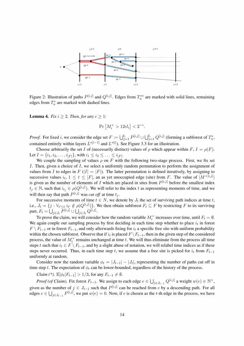
Figure 2: Illustration of paths P [i,j] and Q[i,j]. Edges from T ∗∗u are marked with solid lines, remainingedges from T ∗u are marked with dashed lines.

Lemma 4. Fix i ≥ 2. Then, for any c ≥ 1:

Pr[M+i > 12cli

]< 2−c.

Proof. For fixed i, we consider the edge set F :=⋃lij=1 P

[i,j] ∪⋃lij=1Q

[i,j] (forming a subforest of T ∗u ,contained entirely within layers L∗[i−1] and L∗[i]). See Figure 3.3 for an illustration.

Choose arbitrarily the set I of (necessarily distinct) values of ρ which appear within F , I = ρ(F ).Let I = i1, i2, . . . , i|F |, with i1 ≤ i2 ≤ . . . ≤ i|F |.

We couple the sampling of values ρ on F with the following two-stage process. First, we fix setI . Then, given a choice of I , we select a uniformly random permutation to perform the assignment ofvalues from I to edges in F (|I| = |F |). The latter permutation is defined iteratively, by assigning tosuccessive values it, 1 ≤ t ≤ |F |, an as yet unoccupied edge (site) from F . The value of |M+[i,j]|is given as the number of elements of I which are placed in sites from P [i,j] before the smallest indextj ∈ N, such that itj ∈ ρ(Q[i,j]). We will refer to the index t as representing moments of time, and wewill then say that path P [i,j] was cut off at time tj .

For successive moments of time t ∈ N , we denote by Jt the set of surviving path indices at time t,i.e., Jt = j : ∀t′≤t it′ /∈ ρ(Q[i,j]). We then obtain subforest Ft ⊆ F by restricting F to its survivingpart, Ft =

⋃j∈Jt P

[i,j] ∪⋃j∈Jt Q

[i,j].To prove the claim, we will consider how the random variableM+

i increases over time, until Ft = ∅.We again couple our sampling process by first deciding in each time step whether to place it in forestF \ Ft−1 or in forest Ft−1, and only afterwards fixing for it a specific free site with uniform probabilitywithin the chosen subforest. Observe that if it is placed F \Ft−1, then in the given step of the consideredprocess, the value of M+

i remains unchanged at time t. We will thus eliminate from the process all timesteps t such that it ∈ F \ Ft−1, and by a slight abuse of notation, we will relabel time indices as if thesesteps never occurred. Thus, in each time step t, we assume that a free site is picked for it from Ft−1

uniformly at random.Consider now the random variable φt = |Jt−1| − |Jt|, representing the number of paths cut off in

time step t. The expectation of φt can be lower-bounded, regardless of the history of the process.

Claim (*). E[φt|Ft−1] > 1/3, for any Ft−1 6= ∅.Proof (of Claim). Fix forest Ft−1. We assign to each edge e ∈

⋃j∈Jt−1

Q[i,j] a weight w(e) ∈ N+,given as the number of j ∈ Jt−1 such that P [i,j] can be reached from e by a descending path. For alledges e ∈

⋃j∈Jt−1

P [i,j], we put w(e) = 0. Now, if e is chosen as the t-th edge in the process, we have

14

φt = |Jt−1| − |Jt| = w(e). It follows that:

E[φt|Ft−1] =

∑e∈Ft−1

w(e)

|Ft−1 \ e ∈ F : ρ(e) < it|≥∑

e∈Ft−1w(e)

|Ft−1|≥ |Jt−1|(r[i] − r[i−1])

|Jt−1|(r[i+1] − r[i−1])>

1

3,

which completes the proof of the claim.

Moreover, taking into that φt has bounded range φt ∈ [0, li], and that∑

t∈N φt = li, we obtain aconcentration result on the number of steps until the stopping of the process (Ft = ∅); for completeness,we provide a standalone proof.

Claim (**). For T = 12cli, we have: Pr[FT 6= ∅] < 2−c.

Proof (of Claim). We define the non-negative submartingale Φ′T =∑T

t=1 φ′t as follows. When

Ft−1 6= ∅, we choose φ′t ∈ [0, li] to be dominated by φt, so that φ′t ≤ φt and E[φ′t|Ft−1] = 1/3. (Thelatter condition can always be satisfied by Claim (*)). When Ft−1 = ∅, we put φ′t = 1/3. Observe thatwhen Φ′T > li for some T , we necessarily have φ′t > φt for some t ≤ T , hence FT = ∅. To lower-boundthe probability of the event Φ′T > li, we remark that the bounds φ′t ∈ [0, li] and E[φ′t|Ft−1] = 1/3 implythe following bound on variance of the process: σ2[φ′t|Ft−1] ≤ li/3. Now, using a standard martingalebound (cf. e.g. [17][Thm. 18] applied to the process Xt = Φ′t − t/3), we obtain for any λ > 0:

Pr[Φ′T ≤ T/3− λ] ≤ exp

(−λ2/2

T li/3 + λli/3

).

Substituting T = 12cli and λ = 3cli, we obtain:

Pr[Φ′T ≤ cli] ≤ e−0.9c < 2−c.

Taking into account that c ≥ 1 by assumption, the claim follows directly.

Recalling that in each time step twith Ft 6= ∅, the value of random variableM+i increases by at most

1, we obtain directly from Claim (**) that Pr[M+i > 12cli] < 2−c, which completes the proof.

Next, for 2|i, let Ci ∈ N+ be a random variable defined as the smallest integer such that M+i ≤

12Cili. Since Ci depends only on random values ρ chosen with L∗[i−1] ∪ L∗[i], the random variablesCi2|i are independent. Moreover, by Lemma 4, each Ci may be stochastically dominated by a (inde-pendent) geometrically distributed random variable Γi with parameter p = 1/2. It follows that:∑

2|i,i≤imax

Ci ≤∑2|i,

i≤imax

Γi ∼ NB(bimax/2c, 1/2),

where the parameters of the negative binomial distribution NB(r, p) represent the number of trialswith success probability p until r successes are reached. An application of a rough tail bound forNB(bimax/2c, 1/2) gives:

Pr

∑2|i

Ci < 2imax + 4c lnn

> 1− n−c, for any c > 1. (10)

Recalling that M+i =

∑lij=1 |M+[i,j]| ≤ 12Cili, we may write by concavity of the logarithm function:

li∑j=1

(1 + ln |M+[i,j]|) ≤ li + li ln

1

li

li∑j=1

|M+[i,j]|

≤ li + li ln(12Ci) < li ln(33Ci).

15

We can therefore bound variable N+even, taking into account its definition (8):

N+even =

∑2|i

1≤j≤li

(1 + ln |M+[i,j]|) ≤∑2|i

li ln(33Ci). (11)

We now apply a union bound over the two events given by (9) and (10), which hold w.h.p., From Eq. (9),(10), and (11), we have that for any c > 1, the following event holds w.p. at least 1− 2n−c:

N+even ≤ 3c lnn+ max

(ci)

∑2|i

i≤imax

li ln(33ci), (12)

where (ci)i≤imax,2|i are positive integers satisfying the condition:∑

2|i ci < 2imax + 4c lnn.Returning to Eq. (7), with respect toN+

odd an analogous technique gives us that w.p. at least 1−2n−c:

N+odd ≤ 3c lnn+ max

(ci)

∑26=i

i≤imax

li ln(33ci), (13)

where (ci)i≤imax,2 6| i are likewise positive integers satisfying the condition:∑

26| i ci < 2imax + 4c lnn.Combining Eq. (7) with Eq. (12) and (13) through a union bound (and substituting γi := 33ci), we

eventually obtain that w.p. at least 1− 4n−c:

∑η∈E(T ∗∗u )

X+(η) ≤19∑r=0

|Cut∗(r)u |+ 6c lnn+ max(γi)

∑i≤imax

li ln γi, (14)

where (γi)i≤imax satisfy the condition:

∀iγi ∈ N+ and∑

γi < 132imax + 264c lnn. (15)

Bounding the Sum of X−(η). For the random variables X−(η), the main arguments required toestablish the bound are similar to those in the case of X+(η); we confine ourselves to an exposition ofthe differences. The main difference is that for a path P [i,j], instead of a unique predecessor path Q[i,j]

in layer L∗[i−1], we now have to deal with multiple possible descendant paths in layer L∗[i+1]; on theother hand, the outward-branching structure of the tree means that we can show tighter concentrationbounds in this case.

We recall that P [i] is the set of descending paths P in Tu which stretch precisely between the end-points of the i-th layer, and for 1 ≤ j ≤ li, we denote by R[i,j] the set of all paths in P [i+1] which areextensions of P [i,j], i.e., R[i,j] ⊆ P [i+1] and for all R ∈ R[i,j], we have P [i,j] ⊆ Pu(R+). For the eventX−(η) = 1 to hold, it is now necessary that two conditions are jointly fulfilled: η must satisfy the suffixminimum condition on the path P [i,j]:

η = arg mine∈P [i,j]\Pu(η+)

ρ(e), (16)

and moreover, ρ(η) < maxR∈R[i,j] min ρ(R). We next denote by M−[i,j] ⊆ P [i,j] the set of all edgesη ∈ P [i,j] satisfying ρ(η) < maxR∈R[i,j] min ρ(R). We further denote by η−[i,j,k] the k-th edge inM−[i,j], when ordering edges of M−[i,j] by decreasing distance to the root u, 1 ≤ k ≤ |M−[i,j]|.Finally, we denote by Z−[i,j,k] ∈ 0, 1 the indicator random variable for the event that “edge η−[i,j,k]

satisfies the suffix minimum condition (16) on path P [i,j]”.The subsequent analysis proceeds as before, and we obtain direct analogues of Eq. (7), (8), and (9),

replacing superscripts “+” of all random variables by “−”.We next denote M−i :=

∑lij=1 |M−[i,j]|, for i ≥ 2, and obtain the following analogue of Lemma 4.

16

Lemma 5. Fix i ≥ 2. Then, for any c ≥ 1:

Pr[M−i > 12cli

]< e−4cli < 2−c.

Proof. The proof follows along similar lines as that of Lemma 4.For fixed i, let R[i] :=

⋃lij=1R[i,j]. We consider the edge set F :=

⋃lij=1 P

[i,j] ∪ R[i] (forminga subforest of T ∗u , contained entirely within layers L∗[i] and L∗[i+1]). Choose arbitrarily the set I of(necessarily distinct) values of ρ which appear within F , I = ρ(F ). Let I = i1, i2, . . . , i|F |, withi1 ≤ i2 ≤ . . . ≤ i|F |.

As in the proof of Lemma 4, we couple the sampling of values ρ on F with the following two-stageprocess. First, we fix set I . Then, given a choice of I , we select a uniformly random permutation toperform the assignment of values from I to edges in F (|I| = |F |). The latter permutation is definediteratively, by assigning to successive values it, 1 ≤ t ≤ |F |, an as yet unoccupied edge (site) from F .The value of |M−[i,j]| is given as the number of elements of I which are placed in sites from P [i,j] beforethe smallest index t ∈ N, such that for all paths R ∈ R[i,j], there exists t′ < t such that it′ ∈ ρ(R). Wewill refer to the index t as representing moments of time.

Let R[i] = R1, . . . , R|R[i]|. We say that a path Rk ∈ R[i] was cut off at time t if t is the smallesttime such that it ∈ ρ(Rk). For successive moments of time t ∈ N , we denote by Kt the set of survivingindices k of paths Rk which have not been cut off at time t. We obtain subforest Ft ⊆ F by restrictingF to its surviving part, where we treat a path P [i,j] if it extends to at least one surviving path Rk:

Ft =⋃k∈Kt

Rk ∪⋃j:

∃k∈Kt P[i,j]⊆Pu(R+

k )

P [i,j].

Exactly as in the proof of Lemma 4, we will consider how the random variable M−i increases over time,until Ft = ∅. We again couple our sampling process by first deciding in each time step whether to placeit in forest F \ Ft−1 or in forest Ft−1, and only afterwards fixing for it a specific free site with uniformprobability within the chosen subforest. Observe that if it is placed F \ Ft−1, then in the given step ofthe considered process, the value of M−i remains unchanged at time t. We will thus eliminate from theprocess all time steps t such that it ∈ F \ Ft−1, and by a slight abuse of notation, we will relabel timeindices as if these steps never occurred. Thus, in each time step t, we assume that a free site is pickedfor it from Ft−1 uniformly at random.

Consider now the random variable φt = |Kt−1| − |Kt|, representing the number of paths R cut offin time step t. The expectation of φt can be lower-bounded, regardless of the history of the process.

Claim (*). E[φt|Ft−1] ≥ 1/2, for any Ft−1 6= ∅.Proof (of Claim). Fix forest Ft−1. When inserting it, the number of free sites in layer L∗[i+1] is at

least: ∑k∈Kt−1

|Rk| ≥ |Kt−1|(r[i+1] − r[i]).

On the other hand, since each surviving path P [i,j] extends to some surviving path Rk, the total numberof free sites for insertion of it is upper-bounded by |Kt−1|(r[i+1]− r[i−1]. Since insertion of it into layerL∗[i] means that |Kt| = |Kt−1|, and insertion of it into layer L∗[i+1] means that |Kt| = |Kt−1| − 1, weobtain:

E[φt|Ft−1] ≥ |Kt−1|(r[i+1] − r[i])

|Kt−1|(r[i+1] − r[i−1])≥ 1

2,

which completes the proof of the claim.

Moreover, taking into that φt has bounded range φt ∈ 0, 1, and that∑

t∈N φt ≤ li, we obtain aconcentration result on the number of steps until the stopping of the process (Ft = ∅) directly from the

17

Azuma-McDiarmid martingale inequality (cf. e.g. [17][Thm. 16], [26]). For parameter T = 12cli, weobtain after some transformations:

Pr[F12cli 6= ∅] < e−4cli .

Recalling that in each time step t with Ft 6= ∅, the value of random variable M−i increases by at most 1,we obtain directly that Pr[M−i > 12cli] < e−4cli , which completes the proof.

The rest of the argument proceeds as for the case ofX+, applying Lemma (5) in place of Lemma (4).We eventually obtain the following analogue of Eq. (7): for any c > 1, w.p. at least 1− 4n−c:

∑η∈E(T ∗∗u )

X−(η) ≤19∑r=0

|Cut∗(r)u |+ 6c lnn+ max(γi)

∑i≤imax

li ln γi, (17)

where (γi)i≤imax satisfy condition (15).

Combining Bounds. Introducing the bounds of Eq. (14) and (17) into Eq. (5) through a union boundwe obtain the following statement: For any c > 1, w.p. at least 1− 8n−c:

|S(u)| ≤ 2

19∑r=0

|Cut∗(r)u |+ 12c lnn+ 2 max(γi)

∑i≤imax

li ln γi, (18)

where (γi)i≤imax satisfy condition (15).Now, recalling the bounds on li from Lemma 3, the bound imax < 16 lnD , setting c = 2, and

applying a union bound over all vertices u, we obtain the main technical result of the Section. Wepresent it first in its strongest form, and then provide two more useful corollaries.

Theorem 1. With probability at least 1 − 8/n, all nodes u ∈ V satisfy the following bound on hub setsize:

S(u) ≤ 219∑r=0

|Cut∗(r)u |+ 24 lnn+ 2 max(γi)

∑i=1,2,...,b16 lnDc

li ln γi, (19)

where li ≤ 2 minr∈[r[i+1],r[i+2]] |Cut∗(r)u | with r[i] =

⌈15(

1615

)i⌉, and the maximum is taken over posi-tive integers (γi) satisfying the condition:

∑γi < 2112 lnD +528 lnn.

We provide two more convenient corollaries of Theorem 1. For the case when the considered treesTu are close to scale-free, we simply bound the size of all cuts Cut

∗(r)u through skeleton dimension:

|Cut∗(r)u | ≤ k . Bound (19) then takes the asymptotic form, for imax = b16 lnDc:

S(u) ≤ O(k) +O(log n) +O(k) max(γi)

∑i≤imax

ln γi, (20)

where the latter sum can be bounded using the concavity of the logarithm function as:

max(γi)

∑i≤imax

ln γi ≤ imax max(γi)

ln

1

imax

∑i≤imax

γi

≤ imaxO(max

1, log

log n

logD

)≤

≤ O(

logD max

1, log

log n

logD

).

18

We also observe the following link between the parameters k , D , and n. Since by Proposition 1 graphG has doubling dimension bounded by 2 k +1, it follows that a radius-D ball in G may only contain atmost (2 k +1)dlog2 De nodes from V . Hence, (2 k +1)dlog2De ≥ n, and we obtain:

log n = O(log k · logD). (21)

Thus, the O(log n) additive factor in the bound (20) on S(u) is dominated in notation by the last factorof the sum, which is stated as at least O(k logD).

Combining the above, we obtain the following corollary.

Corollary 2. With probability at least 1−O(1/n), the hub set size of every node is bounded by:

O

(k logD max

1, log

log n

logD

).

In particular, when the graph has sufficiently large diameter, D = nΩ(1), we have that the hub set sizeof all nodes is bounded by O(k logD). For the general case, by introducing Eq. (21) into Corollary 2,we obtain the following statement.

Corollary 3. With probability at least 1−O(1/n), the hub set size of every node is bounded by:

O (k log log k logD) .

When considering the case of trees in which the width of tree T ∗u is far from uniform over differentscales of distance, tighter bounds are obtained by relating the size of S(u) to the integrated skeletondimension k(u). To do this, we apply in Eq. (19) the rough bound: ln γi < ln

∑i γi = O(log log n +

log logD). This leaves us with an expression of the form:

S(u) ≤ O(k(u))+O(log n)+O(log log n+log logD)∑

i≤imax

li ≤ O(log n+k(u)(log log n+log logD)),

where we used the bound∑

i≤imax li ≤ O(k(u)), which follows easily from the definition of the pa-rameter k .

Corollary 4. With probability at least 1−O(1/n), the hub set size of every node u ∈ V is bounded byO(log n+ k(u)(log log n+ log logD)).

4 An Application to δ-preserving Distance Labeling

As a slight extension of our results, we note that our technique based on analyzing tree skeletons forshortest path trees has direct application the δ-preserving distance labeling problem in unweightedgraphs, for some parameter δ > 0. We recall that a scheme is called δ-preserving if for any queriedpair of nodes (u, v) with δ(u, v) > δ, the value returned by the decoder is equal to δ(u, v).

By analogy to the integrated skeleton dimension given by (2), we introduce a variant for this param-eter which only considers cuts at distance more than δ/6.

k δ(u) :=∑

v∈V ∗u :d(u,v)>δ/6

1

du(v)=

∑r∈N,r>δ/6

|Cut∗(r)u |r

. (22)

The claims of Lemma 2 and Corollary 4, which give bounds on average hub size of O(k(u)) andO(log n + k(u)(log log n)) in the unweighted setting, naturally translate to δ-preserving labeling. Forour techniques to be directly applicable, it suffices to subdivide each edge of the graph into a path of 12

19

vertices so that all distances between u − v pairs are divisible by 12, and to choose shortest path treesso that for any pair of nodes u, v, the intersection Tu ∩ Tv contains a shortest u − v path (this may beachieved, for example, by enforcing a unique choice of shortest paths between any node pair, e.g., bychoosing i.a.r. the length of each edge in the range [1− 1/n, 1]). Then, the entire analysis holds, and wecan eventually replace k(u) by k δ(u) in the statement of the claims.

We remark that it is an elementary property of the tree skeleton that |Cut∗(r)u | = O(n/r), since anynode at distance r from u continues in Tu along an independent path of length at least r/2. By perform-ing the latter sum in (22), we obtain k δ(u) = O(n/δ). Thus, we obtain the following Proposition.

Proposition 3. There exists a hub labeling scheme for the δ-preserving distance labeling problem withhubs of average sizeO(n/δ) and worst case sizeO(log n+(n/δ) log log n). The size of the bit represen-tations of the corresponding labels isO((n/δ) log n) andO(log2 n+(n/δ) log n log logn), respectively.

The size of the obtained δ-preserving hub-based labeling scheme is (almost) optimal, since thereholds a lower bound of Ω(n/δ) on both the average and worst-case size of hub sets [10]. In fact, ourscheme can be modified slightly to obtain hub sets of worst-case size O(n/δ) up to a certain thresholdvalue δ = O(

√n). We present the details of this modified scheme in the following Subsection.

4.1 A Modified δ-preserving Labeling Scheme

In this section we present an independent family of distance labeling schemes, which have the δ-preserving property. Whereas the scheme and the presented analysis are valid for any value of parameterδ > 0, we obtain an improvement on the previously discussed scheme only up to some threshold valueδ = O(

√n).

Construction of the Labeling. Fix the value of parameter δ > 0, with 12|δ. The basic building blockof our labeling is a construction of hub sets Sδ(u) for each node u ∈ V , which allow us to handledistance queries for pairs of nodes whose distance is in the range [δ, 5δ/4].

Before providing the details of the constructions of sets Sδ(u), we first introduce some auxiliarynotation. As before, for a pair of nodes u, v ∈ V , we denote by P (u, v) a fixed shortest path between uand v. In the definition of P (u, v), ties between different shortest paths should be broken in a consistentmanner over the whole graph, so that P (u, v) = P (v, u), and the set of shortest paths rooted at a nodeu,⋃v∈V P (u, v), is a spanning tree of G.

For a node u ∈ V , we denote by Tu the shortest path subtree of G, rooted at u, leading from u tonodes at distance in the range [δ, 5δ/4]:

Tu =⋃

v∈V : d(u,v)∈[δ,5δ/4]

P (u, v).

We denote by T ∗u the subtree (skeleton) of tree Tu, also rooted at u and truncated to its first 3δ/4 levelsfrom the root: T ∗u = Tu[v ∈ V (Tu) : d(u, v) ≤ 3δ/4]. We remark that all descending paths in T ∗uhave reach of at least δ/4 in Tu.

The set Sδ(u) will be constructed similarly as before, to include vertices from the central part of anyu−v path in the tree, for vertices v with d(u, v) ∈ [δ, 5δ/4]. However, we wish to control the number ofpossible bad events in which a descending path in the tree T ∗u branches out at some level into too manysubpaths, from each of which some representative node will need be chosen into Sδ(u). To do this, wewill partition the vertex set of tree T ∗u into two subsets, Hu ∪ Lu, known as heavy and light vertices,respectively. A vertex w of T ∗u belongs to Hu if the subtree of T ∗u rooted at w has at least δ leaves (all inthe last level 3δ/4), and belongs to Lu otherwise. We remark that T ∗u [Hu] is a (possibly empty) subtreeof T ∗u , whereas T ∗u [Lu] is a sub-forest of T ∗u , in which each connected component is a tree with less than

20

u

34 δ

54 δ

Hu

δ

Figure 3: Hub set selection for distance range [δ, 5δ/4]. The corresponding shortest path tree Tu for somevertex u is shown in the figure. The set of heavy vertices Hu is shaded around vertex u; all remainingvertices up to distance 3

4δ belong to Lu. Vertices of L′u ⊆ Lu are also marked, with correspondingdescending paths Pd shaded.

δ leaves. In all the considered trees, we maintain the same ancestry relation. In particular, we speak ofa descending subpath in a tree if one of its endpoints is an ancestor of the other with respect to the treeT ∗u rooted at u.

We are now ready to define the hub sets Sδ(u), u ∈ V by the following randomized construction.Assign to each node v ∈ V a real value ρ(v) ∈ [0, 1], uniformly and independently at random. We nowput for all u ∈ V :

Sδ(u) := Hu ∪ L′u, (23)

where L′u ⊆ Lu is defined as the set of all vertices v ∈ Lu, such that there exists a descending subpathPd in T ∗u [Lu], such that v ∈ Pd, |Pd| = δ/12, and v has the minimal value of ρ along path Pd, v =arg minw∈Pd ρ(w) ≡ arg min ρ(Pd). See Fig. 3 for an illustration.

Correctness. We start by showing that sets Sδ have the desired hub property, regardless of the choiceof random values ρ (which may only affect the size of these sets).

Lemma 6. For any pair of nodes u, v ∈ V such that d(u, v) ∈ [δ, 5δ/4], we have:

d(u, v) = minw∈Sδ(u)∩Sδ(v)

(d(u,w) + d(w, v)) .

Proof. Consider the path P = P (u, v) = P (v, u). We have P ⊆ Tu and P ⊆ Tv. Moreover, |P | ≤5δ/4 and |P ∩ T ∗u | = |P ∩ T ∗v | = 3δ/4. Denoting by P ∗ the subpath of P which belongs to both treesT ∗u and T ∗v , P ∗ = P ∩ T ∗u ∩ T ∗v , it follows that |P ∗| ≥ δ/4. We now prove the claim of the lemmaby showing that at least one vertex from P ∗ has to belong to Sδ(u) ∩ Sδ(v). We achieve this by a caseanalysis, depending on the portions of path P ∗ which belong to the sets Lu, Hu, Lv, and Hv.

• If |P ∗∩Hu∩Hv| > 0, then there exists at least one vertexw ∈ P ∗∩Hu∩Hv ⊆ P ∗∩Sδ(u)∩Sδ(v),which completes the proof.

• If |P ∗ ∩ Lu ∩Hv| ≥ δ/12, then there exists at least one descending subpath Pd of length δ/12 inT ∗u [Lu] which is completely contained in P ∗ ∩Hv. Setting w = arg min ρ(Pd), we have w ∈ L′u,and so it follows that w ∈ P ∗ ∩ L′u ∩Hv ⊆ P ∗ ∩ Sδ(u) ∩ Sδ(v).

• If |P ∗ ∩ Hu ∩ Lv| ≥ δ/12, we obtain the result by applying analogous considerations as in theprevious case.

21

• Finally, in all other cases we must have |P ∗ ∩ Lu ∩ Lv| ≥ δ/12. It follows that there exists atleast one subpath Pd ⊆ P ∗ of length δ/12, which is a descending subpath in both T ∗u [Lu] andT ∗v [Lv]. Setting w = arg min ρ(Pd), we obtain w ∈ L′u and w ∈ L′v, hence w ∈ P ∗ ∩L′u ∩L′v ⊆P ∗ ∩ Sδ(u) ∩ Sδ(v).

Analysis. We now consider the size of sets Sδ(u). The size of set Hu is independent of the choice ofrandom variables ρ; it can easily be bounded, taking into account that tree T ∗u has O(n/δ) leaves.

Lemma 7. For all u ∈ V , |Hu| ≤ 3n/δ.

Proof. Let l ∈ Hu be a leaf node of T ∗u [Hu]. By definition of Hu, we have that the subtree of T ∗u rootedat l has at least δ leaves. As every leaf of T ∗u is at depth 3δ/4, and all leaves in tree Tu are at depth atleast δ, it follows that the subtree of l in Tu contains at least δ disjoint descending paths of length δ/4each, and so it has at least δ2/4 nodes. Since the size of tree Tu is at most n, we obtain that tree T ∗u [Hu]has at most 4n/δ2 leaves. Moreover, the distance of each node of T ∗u [Hu] from its root u is at most3δ/4. Hence, |T ∗u [Hu]| ≤ (3δ/4)(4n/δ2) = 3n/δ.

The size of set L′u depends on the choice of random variables ρ. We start by bounding the expectednumber of elements of L′u, belonging to specific connected components of T ∗u [Lu]. Suppose T ∗u [Lu] bea forest consisting of ku trees, and let Lu = L

(1)u ∪ . . . ∪ L(ku)

u be the partition of its vertex set such thatT ∗u [L

(i)u ] represents its i-th connected component. Let l(i)u denote the number of leaves of tree T ∗u [L

(i)u ].

Finally, let L′(i)u = L′u ∩ L(i)u . Clearly, L′(1)

u ∪ . . . ∪ L′(ku)u is a partition of L′u. In the following, we

consider the random variable |L′u| =∑ku

i=1 |L′(i)u |, showing that it has an expectation of O(n/δ), and

obtaining concentration results around this expectation.First, we remark that each descending path of tree T ∗u contributesO(1) elements in expectation to set

T ∗u . Consequently, the expected size of set |L′(i)u | can be related to the number of leaves in the consideredconnected component.

Lemma 8. For all u ∈ V and all 1 ≤ i ≤ ku, E|L′(i)u | ≤ 36l(i)u .

Proof. Let P(i)u be the set of (inclusion-wise) maximal descending paths in the tree T ∗u [L

(i)u ]. We remark

that |P(i)u | ≤ l(i)u .

For a path P ∈ P(i)u , let MP (v) be the event that there exists a subpath Pd ⊆ P , with |Pd| = δ/12,

such that v = arg min ρ(Pd). We have Pr[MP (v)] = 0 for v /∈ P . If v ∈ P , then we use the followingfolklore probability estimation: for MP (v) to hold, one of the two (at most) descending subpaths P ′ ofP of length δ/24, having v as one of their endpoints, must satisfy v = arg min ρ(P ′). It follows that forv ∈ P , we have Pr[MP (v)] ≤ 48/δ. By linearity of expectation we now obtain a bound on E|L′(i)u |:

E|L′(i)u | =∑v∈V

Pr[v ∈ L′(i)u ] ≤∑

P∈P(i)u

∑v∈P

Pr[MP (v)] ≤ |P(i)u | · max

P∈P(i)u

|P | · 48

δ≤ l(i)u ·

3δ

4· 48

δ= 36l(i)u .

By linearity of expectation, we can apply the claim of Lemma 8 over all connected components,obtaining the following result.

Lemma 9. For all u ∈ V , E|L′u| ≤ 144n/δ.

22

Proof. By Lemma 8 we have:

E|L′u| = Eku∑i=1

|L′(i)u | ≤ 36

ku∑i=1

l(i)u .

The claim follows when we observe that∑ku

i=1 l(i)u ≤ 4n/δ. Indeed, this sum represents the total number

of leaves in T ∗u [Lu]. Each such leaf (located at distance 3δ/4 from u) is the upper endpoint of a distinctdescending path of length at least δ/4 in the tree Tu, and |Tu| ≤ n, hence we obtain the bound.

In order to apply Chernoff bounds to the sum of random variables |L′u|, we start by bounding therange of these variables.

Lemma 10. For all u ∈ V and all 1 ≤ i ≤ ku, |L′(i)u | ≤ |L(i)u | < δ2.

Proof. We have L′(i)u ⊆ L(i)u . By the definition of set Lu, tree T ∗u [L

(i)u ] has less than δ leaves and all its

nodes are at distance at most 3δ/4 from its root. It follows that |L(i)u | < δ · 3δ/4 < δ2.

The above upper bound provides an estimate on the maximum value of each random variable |L′(i)u |.However, in order to be able to perform a concentration analysis in a range of fairly large δ (roughly,for n1/3 < δ < n0.5), we also need to bound more tightly the concentration of each |L′(i)u | around itsexpected value.

Let V0 = v ∈ V : ρ(v) < 50 lnnδ . We start by showing that with high probability, all elements of

the sets |L′u| belong to V0.

Lemma 11. Denote by X the “bad” event that there exists a node u ∈ V , such that L′u 6⊆ V0. We have:Pr[X] < 1/n.

Proof. Consider first the probability pv that a fixed node v ∈ V \ V0 satisfies v = arg min ρ(P ), whereP is any fixed path of δ/12 nodes inG which contains v. We have (with the last inequality holding whenδ ≥ 300):

pv =∏

w∈P\v

(1− ρ(v)) = (1− ρ(v))δ/12−1 < (1− 50 lnn/δ)δ/12−1 < n−4.

The probability of event X occurring can be upper-bounded by performing a union bound over allnodes u, all descending paths P in T ∗u [Lu], and all nodes v ∈ P of the event [v = arg min ρ(P )∩v /∈ V0]occurring. For each node u, there are at most n such paths to consider, and less than δ possible nodes vin each path. Overall, we obtain:

Pr[X] ≤ n · n · δ · pv < n3 · n−4 = 1/n.

Next, we show that with high probability, each connected componentL(i)u contains at mostO(δ log n)

nodes from V0.

Lemma 12. Denote by Y the “bad” event that there exists a node u ∈ V and 1 ≤ i ≤ ku, such that|L(i)u ∩ V0| > 100δ lnn. We have: Pr[Y ] < 1/n.

23

Proof. Let Z(v) denote the indicator variable for node v and set V0, i.e., Z(v) = 1 if v ∈ V0 andZ(v) = 0 otherwise. Clearly, Pr[Z(v) = 1] = 50 lnn/δ, and all random variables Z(v), v ∈ V areindependent. For any fixed |L(i)

u |, we have:

E∑v∈L(i)

u

Z(v) ≤ |L(i)u | · 50 lnn/δ ≤ 50δ lnn,

where we used 10 to bound |L(i)u |. Next, we proceed by apply a simple multiplicative Chernoff bound

for the considered random variable:

Pr[|L(i)u ∩ V0| > 100δ lnn] = Pr[

∑v∈L(i)

u

Z(v) > 100δ lnn] ≤ e−50δ lnn/3 < n−16.

Applying a union bound over L(i)u , for all u ∈ V and 1 ≤ i ≤ ku, gives the claim.

We are now ready to apply a Chernoff-bound type analysis to the random variable |L′u|.

Lemma 13. Let δ ≤√n/ lnn. Then: Pr[∀u∈V |L′u| < 800n/δ] = 1−O(1/n).

Proof. Define the random variable λ′(i)u as |L′(i)u | when L′(i)u ⊆ L(i)u ∩ V0 and |L(i)

u ∩ V0| ≤ 100δ lnn,and fix λ′(i)u = 0 otherwise.

Define λ′u =∑ku

i=1 λ′(i)u . All λ′(i)u are independent random variables, since they are functions of

disjoint sets of random variables (ρ(v) : v ∈ L(i)u ). Moreover, we have 0 ≤ λ

′(i)u ≤ 100δ lnn. An

application of a simple multiplicative Chernoff bound gives for any A > 0:

Pr[λ′u ≥ A] <

(eEλ′uA

)A/(100δ lnn)

≤(

144en/δ

A

)A/(100δ lnn)

<

(400n/δ

A

)A/(100δ lnn)

,

where we used the bound Eλ′u ≤ E|L′u| ≤ 144n/δ following from Lemma 9. Putting A = 800n/δ andtaking into account that δ ≤

√n/ lnn, we get for sufficiently large n:

Pr[λ′u ≥ 800n/δ] < 2−8n/(δ2 lnn) <1

n2.

By applying a union bound over all nodes, we obtain that Pr[∀u∈V λ′u < 800n/δ] > 1 − 1/n. Takinginto account Lemmas 11 and 12, we also have:

Pr[∀u∈V λ′u = |L′u|] > 1− 2/n.

Overall, we obtain:Pr[∀u∈V |L′u| < 800n/δ] > 1− 3/n.

In view of the definition of the proposed hub set labeling (Eq. (23)), Lemmas 7 and 13 completethe analysis of the case of δ ≤

√n/ lnn, showing that our randomized construction yields with high

probability hub sets of size O(n/δ) for all nodes of the graph.

Proposition 4. For any 0 < δ ≤√n/ lnn, 12|δ, there exists a hub labeling scheme which correctly

decodes the distance between any pair of nodes lying at a distance in the range [δ, 5δ/4], using hubs ofsize at most O(n/δ).

24

4.2 Improved δ-preserving Distance Labeling for Arbitrary Distance

For an arbitrary instance of the δ-preserving distance labeling problem, we can now construct a hubset S+(u) by combining the results of Propositions 4 and 3, for large and small scales of distance,respectively. Formally, we put:

S+(u) := Sδmax(u) ∪⋃

i=0,1,2,...δi<δmax

Sδi(u), (24)

where in the first part of the expression, the value

δmax = maxδ, b√n/ lnnc

is a suitably chosen threshold parameter, and the hub set Sδmax(u) is constructed following Proposition 4,thus providing a δmax-preserving distance labeling. In the second part of the expression, we take care ofsmaller distances from the range [δ, δmax), by applying Proposition 3 over a specifically chosen distancesequence δii, to obtain hub sets Sδi(u), such that each set Sδi(u) intersects with a shortest u− v path,for all nodes v such that d(u, v) ∈ [δi, 5δi/4]. To obtain a coverage of the entire distance range [δ, δmax),we put δ0 = 12bδ/12c < δ, and choose δi+1 as the largest integer such that 12|δi+1 and δi+1 < 5δi/4.Since the sequence δii is geometrically increasing, in view of Proposition 3, we obtain the followingbound:

|S+(u)| = O(n/δ + |Sδmax(u)|). (25)

Now, taking into account the definition of δmax and bounding |Sδmax(u)| by Proposition 4, we directlyobtain the main result of this Section.

Theorem 2. There exists a δ-preserving distance labeling scheme based on hub sets, such that:

(i) When δ ≤√n/(lnn ln lnn), the hub sets of all nodes are of size O(n/δ), which corresponds to

distance labels of size O(n log δ/δ) per node.

(ii) For any δ > 0, the hub sets of all nodes are of size O(log δ + n log log δ/δ), which correspondsto distance labels of size O

(log2 δ + n log δ log log δ/δ

)per node.

(iii) For any δ > 0, the average size of a hub set, taken over all nodes, is O(n/δ), which correspondsto distance labels of average size O(n log δ/δ) per node.

Furthermore, the corresponding labels can be constructed in expected polynomial time.

5 Computing Skeleton Dimension and Distance Labels

Discrete skeleton representation. Given a tree T rooted at node u with length function `, a discreterepresentation of its skeleton T ∗ can be obtained as the sub-tree with edges vw ∈ E(T ) such thatReachT (v) ≥ 1

2dT (u, v) equipped with length function `′ defined by `′(vw) = `(vw) if ReachT (w) ≥12dT (u,w) and `′(vw) = r − dT (u, v) with r = 2

3(dT (u,w) + ReachT (w)) otherwise. The idea is thatnode w is a leaf of T ∗ that corresponds to the point w′ of edge vw in T that satisfies Reach

T(w′) =

12dT (u,w′). To see this, let x be a descendant of w such dT (w, x) = ReachT (w). We then haver = 2

3dT (u, x). We thus get ReachT

(w′) = dT (v, x) − `′(vw) = dT (u, x) − r = 13dT (u, x) = r

2whereas d

T(u,w′) = dT (u, v) + `′(vw) = r.

25

Skeleton dimension computation. Given a tree T , the reach of each node can be computed by a scanof vertices in reverse topological order. Obtaining the discrete skeleton representation is then straight-forward. Its width k can be computed by scanning vertices by non-decreasing distance from the rootusing a priority queue for storing edges containing nodes in Cutr(T ). This can be done inO(n log log k)time using a dedicated integer priority queue [28].

The skeleton of a graph can thus be simply obtained from an all pair shortest path computation. Withinteger lengths and dedicated priority queues [28], this can be done in O(nm+ n2 log logn) time.

We remark that faster computation of tree skeletons could be obtained in practice by using classi-cal heuristics for bounding reach of nodes [22, 24]. The algorithm proposed in [24] alternates partialshortest-path tree computation with introduction of shortcuts to obtain efficiently reach bounds on thegraph plus the added shortcuts. The computation of partial trees up to a given radius 2r allows to prunenodes with reach less than r. Shortcuts allow to reduce reach of nodes with degree 2: if a node v has twoneighbors u,w, a shortcut uw with length `(uv) + `(vw) is added to by-pass v. The algorithm resultsin reach bounds on the graph with shortcuts. Reach bounds on the original graph can then be obtainedby removing shortcuts in reverse order and updating the reach bound R(v) of a node v by-passed byshortcut uw as R(v) := max(R(v),min(R(u) + `(uv), `(vw) +R(w))) where R(u) and R(w) denotethe reach bounds obtained for u and w respectively. A subtree containing the tree skeleton of a node ucan then be obtained through a partial Dijkstra from u where we prune nodes whose reach is known tobe less than half of the current distance from u. In practice, we believe that this would allow to computeeach skeleton tree in time comparable to an RE query. Our labeling algorithm can then be adapted totake the resulting family of trees as input.

Distance label computation. Computing the hub set of a tree T is more intricate as we have to em-ulate the subdivision of each edge of length a into 12a unweighted edges to conform to the analysis ofSection 3. For the sake of notation, we number these unweighted edges of the subdivision from 1 to12a, and let ρi, 1 ≤ i ≤ 12a, denote the associated random number which is generated for each of theedges of the subdivision. Given a sample ρi | 1 ≤ i ≤ 12a, let M denote the set of indices of edgeswhich are prefix minima or suffix minima in the sequence (ρ1, . . . , ρ12a). For the purpose of our selec-tion algorithm, we only need to generate set M and the ρi-values associated with i ∈ M . We start bygenerating those elements of M which are prefix minima. By a slight abuse of notation, to initialise theprocess, we set i0 = 1 and generate ρ1 uniformly at random in [0, 1], ρ1 := rand(0, 1). For successivej = 0, 1, 2, . . ., we then generate the index ij+1 of the first edge ofM after the edge with index ij (whichis also the first index of M having value less than ρij ). As ij+1 − ij follows a geometric distribution

with parameter p = ρij , this can be done in constant time by setting ij+1 := ij +⌊

log rand(0,1)log(1−p)

⌋(see

e.g. [19]). We then generate ρij+1 uniformly in [0, ρij ]. We generate in this way indices i1, . . . , ix, untilfor some x ∈ N we reach the 12a bound (i.e. ix+1 > 12a). We then proceed similarly in reverse orderfor edges with index greater than ix, to generate those edges with suffix minimal value (note that thistime we have to sample values greater than ρix , rather than greater than 0, and adapt all ranges accord-ingly, for consistency with the choice of prefix minima). In this way, we performO(log a) constant-timesampling operations per edge of length a, obtaining O(log a) values (together with their positions) peredge, in expectation (and also w.h.p. with respect to a). Since random choices made for all edges of theoriginal graph are independent, by a quick Chernoff bound, the total amortized sampling time over thewhole graph is O(m logC), w.h.p., where C denotes the maximum length of an edge. We remark thatwhen constructing a hub set for a subset of nodes, each node only relies on the random choices made inits shortest-path tree, which can be evaluated in time O(n logC), w.h.p.

Our selection algorithm of the edge with minimal value in the middle window for a pair u, v willnecessarily select an edge that we have generated when the window contains a (real) edge extremity.Each time a virtual unweighted edge is selected as a hub, we indeed select the real edge it belongs to.

26

We also have to manage the special case where the middle window entirely falls inside a long edge. Inthat case, the long edge is selected as hub.

The computation of the hub set is then a matter of scanning the tree by non-decreasing distance rof generated vertices while maintaining a sliding middle window for each branch reaching distance r.Using a balanced binary search tree per window for storing the virtual edges it contains, we obtain thehub set in O(n logC log(n logC)) time. Distance labels can thus be computed in expected O(nm +n2 logC(log n + log logC)) time. Note that each of the n labels can be computed independently (e.g.in parallel) in O(m + n logC(log n + log logC)) time per label, as long as randomness is shared (e.g.using random generators with same seeds).

6 Generalizing the Definition of a Skeleton

The definition of a skeleton, and the corresponding notion of skeleton dimension can be generalized intwo ways, by using a different distinct distance metric to compute reach of a point in a tree, as well asby modifying the threshold value of reach required to retain a point in the skeleton.

Using two metrics. Suppose the graph G is associated with two non-negative length functions, ` and`′, of its edges. For example, in road networks, one can typically consider travel time `t and geographicdistance `d, resulting in time and distance metrics, respectively. Another metric which may be of interestis hop count, corresponding to the constant function `h = 1 (i.e. `h(uv) = 1 for each edge uv). Oncea shortest path tree Tu for node u and its geometric realization Tu has been computed according tolength function `, distance and reach within Tu can be computed according to `′. Formally, extendingthe definition from Section 2.1, the skeleton T ∗`

′u of Tu is then defined as the subtree of Tu induced

by v ∈ V (Tu) | Reach`′Tu

(v) ≥ 12d

`′

Tu(u, v), where d`

′

Tuand Reach`

′

Tudenote distance and reach with

respect to `′. The skeleton dimension ofG is then k`′

= maxu∈V (G) Width(T ∗`′

u ). The advantage of thisapproach is that it sometimes results in smaller skeleton dimension (depending on the choice of metric`′), without affecting the correctness of any of the hub labeling schemes designed in this paper. Asan example, the respective skeleton dimensions of the 9-th DIMACS New York graph [1] for differentchoices of metrics turn out to be: k`t = 73, k`d = 66, and k`h = 56, where `t, `d, and `h denote travel-time, geographic-distance, and hop-count length functions, respectively (considering shortest path treesfor the metric `t in all three cases).

We remark that a similar phenomenon, also taking advantage of two metrics, was observed and usedin the reach-pruning approach [24].

Modifying reach threshold. The choice of a reach threshold of 12 in the definition of skeleton is

arbitrary. Indeed, for any fixed α > 0, we can define the skeleton Tα∗u as the subtree of Tu inducedby v ∈ V (Tu) | Reach

Tu(v) ≥ αd

Tu(u, v), and the skeleton dimension kα of G is given as kα =

maxu∈V (G) Width(Tα∗u ). The values of skeleton dimension for different values α and β of the reachthreshold are related to each other by the following Proposition.

Proposition 5. For two constants α < β, the following bounds hold:

kβ ≤ kα ≤ kβk β+1β/α−1

.

Proof. The first relation is immediate since T β∗u is a subtree of Tα∗u for β ≥ α. The second relationis obtained by observing that Cutr(Tα∗u ) ⊆

⋃v∈Cutr′ (T

β∗u )

Cutr−r′(Tβ′∗v ), with r′ = 1+α

1+β and β′ =β+1β/α−1 . Indeed, for w ∈ Cutr(T

α∗u ), we can consider in Tu the point v at distance r′ from u on the

branch leading to w. The reach of w in Tu is then at least r− r′+ReachTu

(v) ≥ r− r′+αr ≥ βr′ for

27

(1 + α)r ≥ (1 + β)r′ and v thus belongs to T β∗u for r′ = 1+α1+β . Moreover, w is at distance r− r′ from v

in Tv and has reach at least αr, implying w ∈ V (T β′∗

v ) for β′ ≤ αrr−r′ , which is the case for β′ = β+1

β/α−1

when r′ = 1+α1+β .

For β = 1 and α < 1, the second relation of the above Proposition gives kα ≤ k1k 2α1−α

, which

also implies that k1 ≤ kα ≤ k21 for α ≥ 1/3. More generally, we can derive the following bounds by

repeatedly applying Proposition 5 for β = 1:

k1 ≤ kα ≤ kdlog(1+1/α)e1 for α < 1.

This shows that for a given graph, skeleton dimension kα grows at most polynomially with 1α .

Naturally, one can also apply both of the above-described generalizations together, obtaining a newskeleton dimension parameter k`

′α with reach metric `′ and reach threshold α. All the results of the

paper about hub labelings and their computation in graphs with low skeleton dimension can be easilygeneralized to use k`

′α instead of k, as long as α < 1 (ensuring that any two skeleton trees T `

′∗αu and

T `′∗αv share a constant fraction of the u− v shortest path). The particular choice of k = k`1/2 was made

with the objective of clarity, and also on account of the simple relationship between k`1/2 and highwaydimension.

7 Conclusion

In this paper, we have proposed skeleton dimension as a measure of the network’s amenability to shortestpath schemes based on hub/transit nodes. We intend it as a parameter which is easy to describe and canbe computed efficiently. Computations of hub sets based on skeleton dimension allow each node toindividually and efficiently define its own hub set, subject only to a universal choice of random id-s.Such a construction is always correct, and gives small hub sets w.h.p. We remark that in a weightednetwork each node can compute its own appropriate labeling in O(m + n logC(log n + log logC))time, where C is the length of the longest integer weight in the network. The definition of hub sets, andthe obtained bounds on their size, hold both for undirected and directed graphs. For directed graphs,skeleton dimension appears to be a parameter which is more directly usable than highway dimension.

Possible extensions of skeleton dimension, discussed in Section 6, include variants of skeleton di-mension with other values of reach threshold, as well as skeleton dimension defined using two separatedistance metrics in the graph: one corresponding to the needs of the shortest path queries (used toconstruct shortest path trees), and another, potentially independent metric used internally in the compu-tation of hub labelings, chosen so as to empirically minimize the width of the skeleton. When studyingaverage-case parameters of a network, the integrated skeleton dimension given by (2) (as well as itsnatural generalizations to weighted graphs) appear to be a natural parameter, which may be related tothat of average highway dimension [3]. We could also use the integrated skeleton dimension averagedover all nodes to get an even more accurate bound on average label size.

Finally, we remark on the interplay between skeleton and highway dimension. Skeleton dimensionis always not greater than geometric highway dimension. We have also shown a clear case of separationin a weighted Manhattan-type network, where skeleton dimension is asymptotically much smaller than(geometric) highway dimension.

We remark that skeleton dimension appears particularly worthy of further theoretical study in thecontext of scale-free models of random graphs (cf. e.g. [9] for a discussion in the context of highwaydimension and reach). For geometric percolation graphs, skeleton dimension displays a close link withthe coalescence exponent for geodesics. Consequently, it may be easier to show rigorous theoreticalbounds for skeleton dimension than for highway dimension.

28

Acknowledgment

The authors thank Przemek Uznanski and Olivier Marty for inspiring discussions on closely relatedproblems. We also thank PU and Zuzanna Kosowska-Stamirowska for their help with the figures.

References

[1] 9th DIMACS Implementation Challenge: The Shortest Path Problem, 2006.

[2] Ittai Abraham, Daniel Delling, Amos Fiat, Andrew Goldberg, and Renato Werneck. Highwaydimension and provably efficient shortest path algorithms. Technical report, September 2013.

[3] Ittai Abraham, Daniel Delling, Amos Fiat, Andrew V. Goldberg, and Renato F. Werneck. VC-dimension and shortest path algorithms. In ICALP, volume 6755 of Lecture Notes in ComputerScience, pages 690–699. Springer, 2011.

[4] Ittai Abraham, Daniel Delling, Andrew V. Goldberg, and Renato F. Werneck. A hub-based labelingalgorithm for shortest paths in road networks. In SEA, volume 6630 of Lecture Notes in ComputerScience, pages 230–241. Springer, 2011.

[5] Ittai Abraham, Daniel Delling, Andrew V. Goldberg, and Renato F. Werneck. Hierarchical hub la-belings for shortest paths. In Proceedings of the 20th Annual European Conference on Algorithms,ESA’12, pages 24–35, Berlin, Heidelberg, 2012. Springer-Verlag.

[6] Ittai Abraham, Daniel Delling, Andrew V. Goldberg, and Renato F. Werneck. Hierarchical hublabelings for shortest paths. In ESA, volume 7501 of Lecture Notes in Computer Science, pages24–35. Springer, 2012.

[7] Ittai Abraham, Amos Fiat, Andrew V. Goldberg, and Renato F. Werneck. Highway dimension,shortest paths, and provably efficient algorithms. In Moses Charikar, editor, Proceedings of theTwenty-First Annual ACM-SIAM Symposium on Discrete Algorithms, SODA 2010, Austin, Texas,USA, January 17-19, 2010, pages 782–793. SIAM, 2010.

[8] Ittai Abraham and Cyril Gavoille. On approximate distance labels and routing schemes with affinestretch. In In International Symposium on Distributed Computing (DISC), pages 404–415, 2011.

[9] David Aldous and Karthik Ganesan. True scale-invariant random spatial networks. Proceedings ofthe National Academy of Sciences, 110(22):8782–8785, 2013.

[10] Stephen Alstrup, Søren Dahlgaard, Mathias Bæk Tejs Knudsen, and Ely Porat. Sublinear distancelabeling. In Piotr Sankowski and Christos D. Zaroliagis, editors, 24th Annual European Symposiumon Algorithms, ESA 2016, August 22-24, 2016, Aarhus, Denmark, volume 57 of LIPIcs, pages 5:1–5:15. Schloss Dagstuhl - Leibniz-Zentrum fuer Informatik, 2016.

[11] Stephen Alstrup, Cyril Gavoille, Esben Bistrup Halvorsen, and Holger Petersen. Simpler, fasterand shorter labels for distances in graphs. In Robert Krauthgamer, editor, Proceedings of theTwenty-Seventh Annual ACM-SIAM Symposium on Discrete Algorithms, SODA 2016, Arlington,VA, USA, January 10-12, 2016, pages 338–350. SIAM, 2016.

[12] Maxim A. Babenko, Andrew V. Goldberg, Anupam Gupta, and Viswanath Nagarajan. Algorithmsfor hub label optimization. In Fedor V. Fomin, Rusins Freivalds, Marta Z. Kwiatkowska, andDavid Peleg, editors, Automata, Languages, and Programming - 40th International Colloquium,ICALP 2013, Riga, Latvia, July 8-12, 2013, Proceedings, Part I, volume 7965 of Lecture Notes inComputer Science, pages 69–80. Springer, 2013.

29

[13] H. Bast, Stefan Funke, Domagoj Matijevic, Peter Sanders, and Dominik Schultes. In transit toconstant time shortest-path queries in road networks. In ALENEX. SIAM, 2007.

[14] Holger Bast, Stefan Funke, Peter Sanders, and Dominik Schultes. Fast routing in road networkswith transit nodes. Science, 316(5824):566–566, 2007.

[15] Reinhard Bauer and Daniel Delling. SHARC: Fast and robust unidirectional routing. J. Exp.Algorithmics, 14:4:2.4–4:2.29, January 2010.

[16] Bela Bollobas, Don Coppersmith, and Michael Elkin. Sparse distance preservers and additivespanners. SIAM Journal on Discrete Mathematics, 19(4):1029–1055, 2005.

[17] Fan R. K. Chung and Lincoln Lu. Survey: Concentration inequalities and martingale inequalities:A survey. Internet Mathematics, 3(1):79–127, 2006.

[18] Edith Cohen, Eran Halperin, Haim Kaplan, and Uri Zwick. Reachability and distance queries via2-hop labels. SIAM J. Comput., 32(5):1338–1355, May 2003.

[19] Luc Devroye. Non-Uniform Random Variate Generation. Springer-Verlag, 1986.

[20] Andreas Emil Feldmann, Wai Shing Fung, Jochen Konemann, and Ian Post. A 1 + ε-embeddingof low highway dimension graphs into bounded treewidth graphs. In ICALP 2015, volume 9134of Lecture Notes in Computer Science, pages 469–480. Springer, 2015.

[21] Cyril Gavoille, David Peleg, Stephane Perennes, and Ran Raz. Distance labeling in graphs. J.Algorithms, 53(1):85–112, October 2004.

[22] Andrew V. Goldberg, Haim Kaplan, and Renato F. Werneck. Reach for A*: Efficient point-to-pointshortest path algorithms. In ALENEX, pages 129–143. SIAM, 2006.

[23] R.L. Graham and H.O. Pollak. On embedding graphs in squashed cubes. In Y. Alavi, D.R. Lick, andA.T. White, editors, Graph Theory and Applications, volume 303 of Lecture Notes in Mathematics,pages 99–110. Springer Berlin Heidelberg, 1972.

[24] Ronald J. Gutman. Reach-based routing: A new approach to shortest path algorithms optimizedfor road networks. In ALENEX/ANALCO, pages 100–111. SIAM, 2004.

[25] Ekkehard Kohler, Rolf H. Mohring, and Heiko Schilling. Fast point-to-point shortest path compu-tations with arc-flags. In 9th DIMACS Implementation Challenge, 2006.

[26] Colin McDiarmid. Concentration. In Michel Habib, Colin McDiarmid, Jorge Ramirez-Alfonsin,and Bruce Reed, editors, Probabilistic Methods for Algorithmic Discrete Mathematics, pages 195–248. Springer Berlin Heidelberg, 1998.

[27] Igor Nitto and Rossano Venturini. On compact representations of all-pairs-shortest-path-distancematrices. In Paolo Ferragina and Gad M. Landau, editors, Combinatorial Pattern Matching, 19thAnnual Symposium, CPM 2008, Pisa, Italy, June 18-20, 2008, Proceedings, volume 5029 of Lec-ture Notes in Computer Science, pages 166–177. Springer, 2008.

[28] Mikkel Thorup. Integer priority queues with decrease key in constant time and the single sourceshortest paths problem. Journal of Computer and System Sciences, 69(3):330 – 353, 2004.

[29] Oren Weimann and David Peleg. A note on exact distance labeling. Inf. Process. Lett.,111(14):671–673, 2011.

30