1

Using AutoDock with

AutoDockTools: A Tutorial

Written by Ruth Huey and Garrett M. Morris

The Scripps Research Ins ti tute Molecular Graphics Labora tory

10550 N. Torrey Pines Rd. La Jolla, California 92037-1000

USA

3 August 2006

2

Contents

Contents .......................................................................... 2

Introduction ..................................................................... 4 Before We Start….............................................................................4

FAQ – Frequently Asked Questions ..................................... 5

Exercise One: PDB Fi les are Not Perfect: Edit ing a PDB fi le ... 7 Procedure: .......................................................................................7

Exercise Two: Preparing a l igand f i le for AutoDock. ............ 11 Procedure: .....................................................................................11

Exercise Three: Preparing the macromolecule f i le. .............. 15 Procedure: .....................................................................................15

Exercise Four: Preparing the grid parameter f i le. ................ 17 Procedure: .....................................................................................17

Exercise Five: Start ing AutoGrid ....................................... 20 Procedure: .....................................................................................20

Exercise Six: Preparing the docking parameter f i le. ............. 22 Procedure: .....................................................................................22

Exercise Seven: Start ing AutoDock. .................................. 24 Procedure: .....................................................................................24

Exercise Eight : Analyzing AutoDock Results -Reading Docking Logs .............................................................................. 26

Procedure: .....................................................................................26

Exercise Nine: Analyzing AutoDock Results -Visualizing Docked Conformations ................................................................ 29

Procedure: .....................................................................................29

Exercise Ten: Analyzing AutoDock Results -Clustering Conformations ................................................................ 31

Procedure: .....................................................................................31

Two Step QA Analysis of AutoDock Results ......................... 34

3

Exercise Eleven: Analyzing AutoDock Results -Visualizing Conformations in Context ................................................. 36

Procedure: .....................................................................................36

Files for exercises: .......................................................... 40 Input Files:......................................................................................40 Results Files ....................................................................................40 Useful Scripts..................................................................................40 Customization Options for ADT ........................................................40

Appendix 1: Docking Parameters ...................................... 41 Parameters common to SA, GA, GALS: ............................................41 Simulated Annealing Specific Parameters:.........................................43 Genetic Algorithm Specific Parameters: ............................................44 Local Search Specific Parameters: ....................................................45 Clustering keywords:.......................................................................46

Appendix 2: Conformation Player ..................................... 47

4

Introduction

This tutorial will introduce you to docking using the AutoDock suite of programs. We will use a Graphical User Interface called AutoDockTools, or ADT, that helps a user easily set up the two molecules for docking, launches the external number crunching jobs in AutoDock, and when the dockings are completed also lets the user interactively visualize the docking results in 3D.

Before We Start…

And only if you are at The Scripps Research Institute… These commands are for people attending the tutorial given at Scripps. We will be starting the graphical user interface to AutoDock from the command line. To do this, you need to open a Terminal window and then type this at the UNIX, Mac OS X or Linux prompt:

% alias adt /mgl/prog/share/bin/adt14

% source /tsri/python/share/bin/initadt_v2.csh

% limit stacksize unlimited

% cd tutorial

% adt

5

FAQ – Frequently Asked Questions

1. Where should I start ADT? You should always start ADT in the same directory as the macromolecule and ligand files. You can start ADT from the command line in a Terminal by typing “adt” and pressing <Return> or <Enter>.

2. Should I always add polar hydrogens? Yes, for the macromolecule you should always add polar hydrogens and then assign Kollman United Atom charges. For the ligand, you should add all hydrogens before computing Gasteiger charges, and then you must merge the non-polar hydrogens. If your ligand is a peptide, instead you can ust add polar hydrogens and assign Kollman United Atom charges. Polar hydrogens are hydrogens that are bonded to electronegative atoms like oxygen and nitrogen. Non-polar hydrogens are hydrogens bonded to carbon atoms.

3. How many AutoGrid grid maps do I need? You need one AutoGrid map for every atom type in the ligand plus an electrostatics map. E.g.: for ethanol, C2H5OH, you would need C, O and H maps plus an ‘e’ map.

4. Why should all the total charges on the residues be an integer? This is because it is assumed that the residue is interchangeable with others, and that no electrons are withdrawn or received by adjacent residues. In proteins, e.g., arginines should have a total charge of +1.000 if they are protonated, or 0.000 if they are neutral.

5. How easy will it be to get good docking results? In general, the more rotatable bonds in the ligand, the more difficult it will be to find good binding modes in repeated docking experiments.

6

6. How big should the AutoGrid grid box be? The grid volume should be large enough to at least allow the ligand to rotate freely, even when the ligand is in its most fully-extended conformation.

7. Can I identify potential binding sites of a ligand on a protein with AutoDock? Yes, if you do not know where the ligand binds, you can build a grid volume that is big enough to cover the entire surface of the protein, using a larger grid spacing than the default value of 0.375Å, and more grid points in each dimension. Then you can perform preliminary docking experiments with AutoDock to see if there are particular regions of the protein that are preferred by the ligand. This is sometimes referred to as “blind docking”. Then, in a second round of docking experiments, you can build smaller grids around these potential binding sites and dock in these smaller grids. If the protein is very large, then you can break it up into overlapping grids and dock into each of these grid sets, e.g. one covering the top half, one covering the lower half, and one covering the middle half.

7

Exercise One: PDB Files are Not Perfect: Editing a PDB file

Protein Data Bank (PDB) files can have a variety of potential problems that need to be corrected before they can be used in AutoDock. These potential problems include missing atoms, added waters, more than one molecule, chain breaks, alternate locations etc.

AutoDockTools (ADT) is built on the Python Molecule Viewer (PMV), and has an evolving set of tools designed to solve these kinds of problems. In particular, two modules, editCommands and repairCommands, contain many useful tools which permit you to add or remove hydrogens, repair residues by adding missing atoms, modify histidine protonation, modify protonation of intrachain breaks, etc.

In this exercise, you will work on the macromolecule, the molecule we want to dock to and which will be kept fixed during the dockings. You will learn how to remove waters, how to add the polar hydrogens that AutoDock expects, and how to save the modified result.

Procedure:

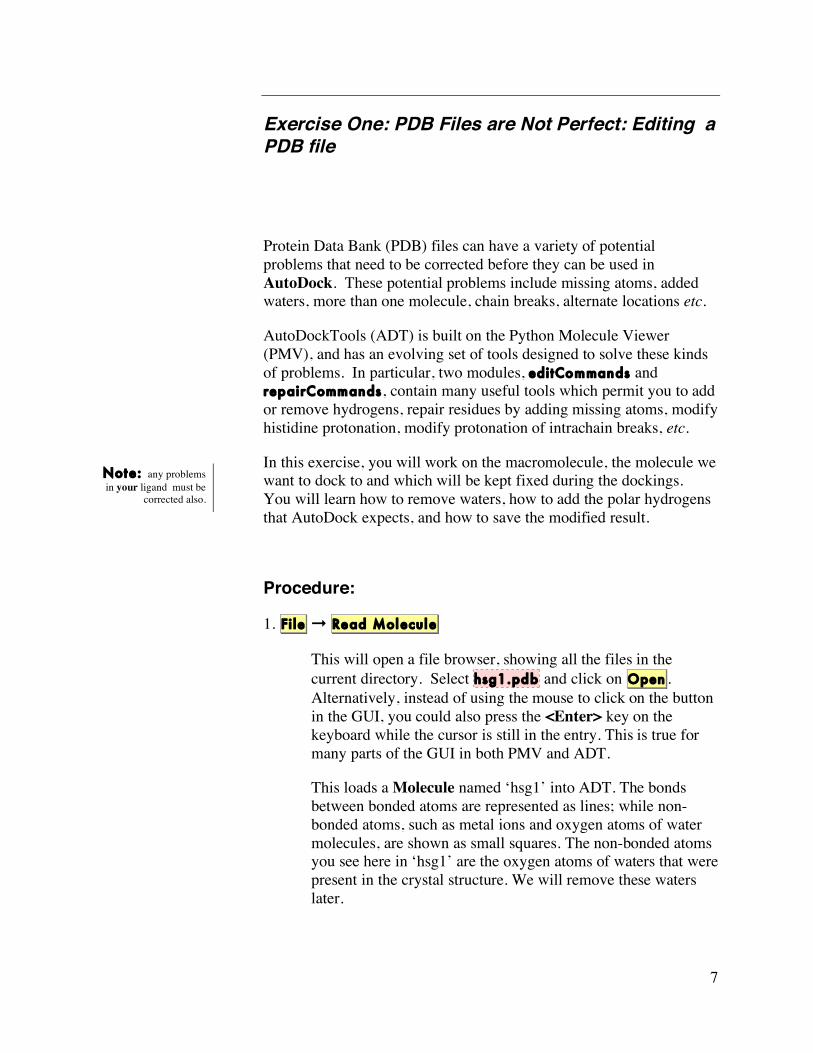
1. File ➞ Read Molecule

This will open a file browser, showing all the files in the current directory. Select hsg1.pdb and click on Open . Alternatively, instead of using the mouse to click on the button in the GUI, you could also press the <Enter> key on the keyboard while the cursor is still in the entry. This is true for many parts of the GUI in both PMV and ADT.

This loads a Molecule named ‘hsg1’ into ADT. The bonds between bonded atoms are represented as lines; while non-bonded atoms, such as metal ions and oxygen atoms of water molecules, are shown as small squares. The non-bonded atoms you see here in ‘hsg1’ are the oxygen atoms of waters that were present in the crystal structure. We will remove these waters later.

Note: any problems in your ligand must be

corrected also.

8

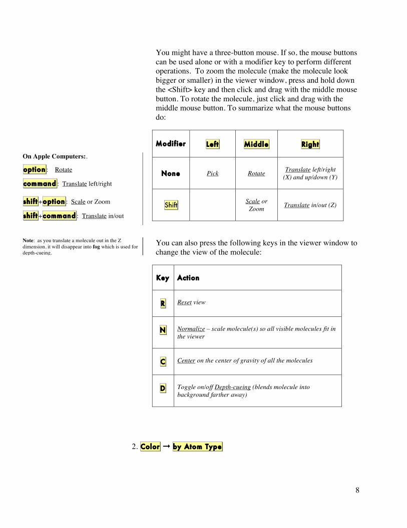
You might have a three-button mouse. If so, the mouse buttons can be used alone or with a modifier key to perform different operations. To zoom the molecule (make the molecule look bigger or smaller) in the viewer window, press and hold down the <Shift> key and then click and drag with the middle mouse button. To rotate the molecule, just click and drag with the middle mouse button. To summarize what the mouse buttons do:

Modif ier

Left

Middle

Right

None Pick Rotate Translate left/right (X) and up/down (Y)

Shift Scale or Zoom Translate in/out (Z)

You can also press the following keys in the viewer window to change the view of the molecule:

Key Action

R Reset view

N Normalize – scale molecule(s) so all visible molecules fit in the viewer

C Center on the center of gravity of all the molecules

D Toggle on/off Depth-cueing (blends molecule into background farther away)

2. Color ➞ by Atom Type

On Apple Computers:.

option : Rotate

command : Translate left/right shif t +option : Scale or Zoom

shif t +command : Translate in/out

Note: as you translate a molecule out in the Z dimension, it will disappear into fog which is used for depth-cueing.

9

Click on All Geometries and then click OK . All of the displayed objects will be colored according to the chemical element, as follows:

❍ Carbons that are aliphatic (C) - white, ● Carbons that are aromatic (A) - green, ● Nitrogens (N) - blue, ● Oxygens (O) - red, ● Sulfurs (S) - yellow, ● Hydrogens (H) - cyan.

This makes the display more informative.

3. Select ➞ Select From String

Select From String lets you build a selection based on strings you enter for the Molecule, Chain, Residue and/or Atom level. These strings can be names, numbers, ranges of numbers, or lambda expressions which are evaluated to build a set. The strings can contain regular expressions including wild cards such as * which matches anything. For our example, we want to select all atoms (*) in residues named HOH*. Type HOH* in the Residue entry, press the <Tab> key to move to the next entry field, and type * in the Atom entry. Now click Add . You may get a warning asking you if you want to “change selection level to Atom”: if so, click Yes .

You will see Selected: 127 Atom(s) with a yellow background in the center of the message-bar at the bottom of the ADT window. Click Dismiss to close the Select From String widget.

4. Edit ➞ Delete ➞ Delete AtomSet

If there is a current selection, it is deleted by this command. You will be asked if you really want to do this, because deleting an AtomSet (or a molecule) cannot be undone. Click on CONTINUE . The selected oxygens will disappear from the viewer.

Note: if there is no current selection, ADT expands the selection to include all atoms

in the viewer. If the userpref, ‘warnOnEmptySelection’ is set to 1, ADT

will ask you if it should “expand empty selection to all molecules.” The default

behavior is to not ask you if you want the empty selection to be expanded to include

every molecule in the viewer. For ADT, make sure to leave the

warnOnEmptySelection set to 0.

10

5. Edit ➞ Hydrogens ➞ Add

Choose to add Polar Only using Method noBondOrder with yes to renumbering. Click OK to add the polar hydrogens. 330 hydrogen atoms are added to hsg1.

Step 6 is optional because we are going to add charges and atomic solvation parameters to hsg1 in Exercise Three. However, if you had no further plans to modify this molecule, you would save your modified result at this point:

[6. Fi le ➞ Save ➞ Write PDB

This opens a Write Options widget that lets you enter various options including Filename. Type in hsg1.pdb. You can choose which if any types PDB records to write (default is to write ATOM and HETATM records only, whether to Sort Nodes and whether to Save Transformed Coords. Choose Sort Nodes but leave all the other check-buttons off so that no CONECT records are written. Click on OK to write the file.]

Note: The added hydrogens are automatically saved as a set

“hsg1_addedH” which you could select with the sequence:

Select ➞ Select a set , hsg1_addedH, OK

If you try this, be sure to clear the selection using the pencil eraser

icon before you go on.

11

Exercise Two: Preparing a ligand file for AutoDock.

AutoDock ligands have partial atomic charges for each atom. We also distinguish between aliphatic and aromatic carbons: names for aromatic carbons start with ‘A’ instead of ‘C’. AutoDock ligands are written in files with special keywords recognized by AutoDock. The keywords ROOT, ENDROOT, BRANCH, and ENDBRANCH establish a “torsion tree” object or torTree that has a root and branches. The root is a rigid set of atoms, while the branches are rotatable groups of atoms connected to the rigid root. The keyword TORSDOF signals the number of torsional degrees of freedom in the ligand. The TORSDOF for a ligand is the total number of possible torsions in the ligand minus the number of torsions that only rotate hydrogens. TORSDOF is used in calculating the change in free energy caused by the loss of torsional degrees of freedom upon binding.

You can follow what happens with the ligand more easily if you undisplay the macromolecule first. To do this, click on Display ➞ Show/Hide Molecule . Click on the check-button labelled ❑ hsg1:ON/OFF to undisplay hsg1. Close the widget by clicking on the X in the top right corner of the widget (or the left-most red circle at the top).

Procedure:

1. Ligand ➞ Input ➞ Open..(AD3)

Opens a file browser. Click on the PDBQ fi les: (*.pdbq) menu button to display file type choices and click on PDB fi les: (* .pdb) files. Choose ind.pdb . Click on Open .

After the ligand is loaded in the viewer, ADT initializes it. This process involves a number of steps:

• ADT checks for and merges non-polar hydrogens, unless you have set a userpref ‘adt_automergeNPHS’ not to do so.

• ADT detects whether the ligand already has charges or not. If not, ADT determines whether the ligand is a peptide, by checking whether all of its residues’ names appear in the

Note: you must always add hydrogens to the ligand before you select it to be the ligand.

.

12

standard set of the 20 commonly occurring amino acids. If all the residues are amino acids, ADT adds Kollman charges to the ligand. If not, it computes Gasteiger charges; remember that for the Gasteiger calculation to work correctly, the ligand must have all hydrogen atoms added, including both polar and non-polar ones. If the charges are all zero, ADT will try to add charges. It checks whether the total charge per residue is an integer. Kollman charges are added using a look-up dictionary based on the names of the atoms in the ligand. If the name is not found, a charge of 0.0 is assigned.

• ADT renames planar carbons unless you have set a user preference, ‘autotors_autoCtoA’ not to do so. For peptide ligands, ADT uses a look-up dictionary for planar cyclic carbons (unless you set another userpref, ‘autotors_use ProteinAromaticList’, not to do so). For other ligands, ADT determines which are planar cyclic carbons by calculating the angle between adjacent carbons in the ring. If the angle is less than the cut-off of 7.5° (the default value) for all the atoms in the ring, the first letter of the ring carbons’ atom names will be renamed “A”.

• ADT displays a summary for the formatted ligand which lists what type of changes were added, how many non-polar hydrogens, aromatic carbons and rotatable bonds were found, the number of torsional degrees of freedom detected (TORSDOF) and the amount the total charge differed from an integral value (total charge error). Click on OK to close the summary.

2. Ligand ➞ Torsion Tree ➞ Detect Root…

ADT determines which atom fits its idea of the best root and marks it with a green sphere.

This best root is the atom in the ligand with the smallest largest subtree. In the case of a tie, if either atom is in a cycle, it is picked to be root. If neither atom is in a cycle, the first found is picked. (If both are in a cycle, the first found is picked). As you might imagine, this can be a slow process for large ligands.

The rigid portion of the molecule includes this root atom and all atoms connected to it by non-rotatable bonds (which we will examine in the next section.) You can visualize the current

Note: it is also possible to edit which planar, cyclic carbons are renamed ‘A’ but we are not going to do that in this example. Also you can adjust the aromaticity cut-off if a ring is more warped via Ligand ➞ Aromatic Carbons � ➞ � Aromaticity Criterion .

13

root portion with Ligand ➞ Torsion Tree ➞ Show Root Expansion (and hide this with Ligand ➞ Torsion Tree ➞ Show/Hide Root Marker ) However, at this point in our example, the root portion includes only the best root atom, atom C11, because all its bonds to other atoms are rotatable.

3. Ligand ➞ Torsion Tree ➞ Choose Torsions…

Opens the Torsion Count widget. The widget displays the number of currently active bonds. Bonds which cannot be rotated are colored red. Bonds which could be rotated but are currently marked as inactive are colored purple. Bonds which are currently active are colored green.

Bonds in cycles cannot be rotated. Bonds to leaf atoms cannot be meaningfully rotated. Only single bonds can be rotated (not double or aromatic etc…). ADT determines which bonds could be rotated (‘possibleTors’). You set which of these are to be rotatable (‘activeTors’) by inactivating the others

You can toggle the activity of a bond or group of bonds by picking them in the viewer. Alternatively, buttons on this widget let you toggle the activity of a type of bonds such as ‘peptide bonds’, ‘amide bonds’, ‘bonds between selected atoms’ or ‘all rotatable bonds’. One way to do this is to click on Make all act ive bonds non-rotatable then click on Make all rotatable bonds rotatable .

Amide bonds should not be rotatable. By default, amide bonds amide bonds are treated as non-rotatable. You can see that two bonds have been inactivated, the bond between atoms N2;6 and C3;4 and that between atoms C21;26 and N4:28. Notice that the current total number of rotatable bonds is 14. You could reactivate these bonds by clicking on Make all amide bonds rotatable If you do, be sure to inactive them before the next step.

Before you close this widget with Done , leave all the bonds except the two amide bonds active. 14/32 on the widget indicates that 14 are currently active out of the maximum allowed by AutoDock which is 32.

Note: CAUTION! Trying to make all bonds between selected atoms inactive when there is no specific selection in ind will cause an error because then the selection is expanded to include everything and ADT will try to change the activity of bonds in hsg1.

14

4.Ligand ➞ Torsion Tree ➞ Set Number of Torsions…

This feature allows you to set the total number of active bonds while specifying whether you want active bonds which move the fewest atoms or those which move the most. To see this distinction, set the radiobutton for fewest atoms , type ‘6’ in the entry and then press <Enter> on your keyboard. ADT will turn off all but six torsions, leaving active the torsions which move the fewest atoms.

Set the radiobutton to most atoms and type <Enter> in the entry window. You will see a very different set of 6 rotatable bonds.

For our exercise, leave the 6 torsions that move the fewest atoms active. Click Dismiss to close the widget.

5. Ligand ➞ Output ➞ Save as PDBQ…(AD3)

Opens a file browser allowing you to enter a name. Type in ‘ind.out.pdbq’ and click Save .

You must write a pdbq file, which is an AutoDock specific file format, pdb augmented by ‘q’, a charge. Our convention is to name the ligand output files ‘*.out.pdbq’, but this is not required.

Note: This step, using Set Number of

Active Torsions is optional. We are

including it so that your ligand will always have

the same torsion tree with only a few torsions for

this tutorial

15

Exercise Three: Preparing the macromolecule file.

The receptor file used by AutoDock must be in pdbqs format which is pdb plus ‘q’ charge and ‘s’ solvation parameters: AtVol, the atomic fragmental volume, and AtSolPar, the atomic solvation parameter which are used to calculate the energy contributions of desolvation of the macromolecule by ligand binding.

If the molecule from Exercise One is not still in your viewer, repeat Exercise One. Undisplay the ligand using Display ➞ Show/Hide Molecule .

Procedure:

1. Grid ➞ Macromolecule ➞ Choose…(AG3)

Choose hsg1 .

Selecting the macromolecule in this way causes the following sequence of initialization steps to be carried out automatically:

• ADT checks that the molecule has charges. If not, ADT determines whether it is a peptide. If so, ADT adds Kollman charges; if not, it adds gasteiger charges. ADT checks that the total charge per residue is an integer. If not, a list of residues with non-integral charges pops up.* ADT also adds solvation parameters,. This process, like that of adding Kollman charges, depends on a look-up dictionary based on the names of the atoms and the name of their parent residues. If a name is not found, 0.0 is assigned for each parameter.

• ADT merges non-polar hydrogens unless the userpref adt_automergeNPHS is set not to do so.

• ADT also determines the types of atoms in the macromolecule. AutoDock can accommodate up to 7 atom types in the macromolecule. It uses a standard set with two customizable types, ‘X’ and ‘M’. If your macromolecule has a non-standard atom type, ADT will prompt you to set up a customizable type X or M for it by entering energy parameters. For example, Zn is not in the standard set. If your

* Note: the most likely cause of non-integral charges using our tutorial

example hsg1 is that it lacks polar hydrogens (see Exercise One). With

other molecules, it is also possible that some atoms are missing from the pdb

file. You can repair these missing atoms with a command in the

repairCommands module. To do so, first load that module then

Edit ➞Misc➞Repair Missing Atoms . Obviously, you have to repeat

Exercise One: adding polar hydrogens etc if any residues have been repaired.

16

macromolecule has Zn, for AutoDock you have to rename the ‘Zn’ as ‘M’ and provide energy coefficients for Zn. ‘X’ can be used as a second customizable type. It is not possible to have more than 7 types in the macromolecule.

The macromolecule must be written in a pdbqs file for use by AutoGrid. Since the molecule you chose has been modified by ADT, a file browser opens for you to specify a file name. Type hsg1.pdbqs in the input entry and click Save .

17

Exercise Four: Preparing the grid parameter file.

The grid parameter file tells AutoGrid the types of maps to compute, the location and extent of those maps and specifies pair-wise potential energy parameters. In general, one map is calculated for each element in the ligand plus an electrostatics map. Self-consistent 12-6 Lennard-Jones energy parameters - Rij, equilibrium internuclear separation and epsij, energy well depth - are specified for each map based on types of atoms in the macromolecule. If you want to model hydrogen bonding, this is done by specifying 12-10 instead of 12-6 parameters in the gpf.

Procedure:

1. Grid ➞ Set Map Types

The types of maps depend on the types of atoms in the ligand. Thus one way to specify the types of maps is by choosing a ligand. If the ligand you formatted in Exercise Two is still in the viewer, choose Grid ➞ Set Map Types ➞ Choose Ligand…(AG3) . If not, use Grid ➞ Set Map Types ➞ Open Ligand…(AG3) .

Choosing the ligand opens the AutoGpf Ligand widget that allows you to modify the types of maps to be calculated, and to choose whether to model possible hydrogen bonding. In our example, the ligand has Nitrogen, Oxygen and Hydrogen atoms so we can model N-H and O-H hydrogen bonds but not S-H hydrogen bonds.

Close this widget with the Accept button.

2. Grid ➞ Grid Box…

Opens the Grid Options Widget. First a brief tour of this widget:

• This has menu buttons at the top: File , Center , View and Help .

Note: Alternatively, if you plan to use the same macromolecule with a variety of different ligands, you might choose

to calculate all the maps you would eventually need via

Set Map Types -> Directly .

18

➞ File

This menu lets you close the Grid Options Widget, which also causes the grid box to disappear. You can Close saving current values to keep your changes or Close w/out saving to forget your changes.

➞ Center

This menu lets you set the center of the grid box in four ways: ➞ Pick an atom , ➞ Center on l igand , ➞ Center on macromolecule or ➞ On a named atom .

➞ View

This menu allows you to change the visibility of the box using Show box , and whether it is displayed as lines or faces, using Show box as l ines . This menu also allows you to show or hide the center marker using Show center marker and to adjust its size using Adjust marker size .

• The “Grid Options Widget” displays the Current Total Grid Points per map. This tells you how big each grid map will be: (nx + 1) x (ny + 1) x (nz + 1), where nx is the number of grid points in the x-dimension, etc.

• This has 3 thumbwheel widgets which let you change the number of points in the x, y and z dimensions. The default settings are 40, 40, 40 which makes the total number of grid pts per map 68921 because AutoGrid always adds one in each dimension.

• You will also notice it has a thumbwheel that lets you adjust the spacing between the grid points.

• There are also entries and thumbwheels that let you change the location of the center of the grid.

The number of points in each dimension can be adjusted up to 126. AutoGrid requires that the input number of grid points be an even number. It then actually adds one point in each dimension, since AutoGrid and AutoDock need a central grid point.

Note: clicking with the right mouse button on a thumbwheel

widget opens a box that allows you to type in the desired value directly. Like many other entry fields in ADT, this updates only

when you press <Enter>.

19

The spacing between grid points can be adjusted with another thumbwheel. The default value is 0.375 Å between grid points, which is about a quarter of the length of a carbon-carbon single bond. Grid spacing values of up to 1.0 Å can be used when a large volume is to be investigated. If you were to need grid spacing values larger than this, you could edit the GPF in a text editor before running AutoGrid.

For this exercise:

Adjust the number of points in each dimension to 60 . Notice that each map will have 226,981 points.

Type in 2.5 , 6.5 and -7.5 in the x center, y center and z center entries. This will center the grid box on the active site of the HIV-1 protease, hsg1.

Close this widget by clicking File ➞ Close saving current .

3. Grid ➞ Output ➞ Save GPF…(AG3)

Opens a file browser allowing the user to specify the name of the grid parameter file. The convention is to use ‘.gpf’ as the extension.

Write the gpf as ‘hsg1.gpf’

[4. Grid ➞ Edit GPF…

If you have written a grid parameter file, it opens in an editing window. If not, you can pick one to read in and edit via the Read button. If you make any changes to the content of the grid parameter file, you can save the changes via the Write button. Edit GPF will open the file we wrote in step 3. Either OK or Cancel close this widget]

Important Note: z value is NEGATIVE 7.5

20

Exercise Five: Starting AutoGrid

In general you should know:

AutoGrid (and AutoDock) must be run in the directories where the macromolecule, ligand and parameter files are to be found.

The named files in the parameter file must not include pathnames.

Currently, it is not possible to run either program on a WINDOWS platform except in a cygwin shell.

Procedure:

Run ➞ Run AutoGrid…

Opens the Run AutoGrid widget. Here is a brief tour:

The first two entries in the widget are used to specify which machine to use. By default the local machine is named in the Macro Name: entry and in the Host name: entry. It is possible to define macros to specify other machines with Run -> Host Preferences…

Program Pathname: entry specifies the location of the autogrid3 executable. If it is not in your path, you can use the Browse button to locate it.

Parameter Filename: entry specifies the gpf file. If you have just written a gpf file, opening this widget will automatically load the gpf filename in the Parameter Filename: entry. If not, you can use the Browse button to the right of the entry to locate the gpf you want to use.

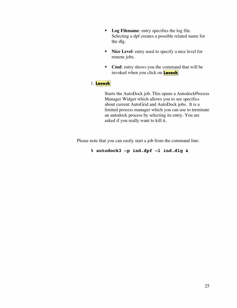
Log Filename: entry specifies the log file. Selecting a gpf creates a possible related name for the glg.

21

Nice Level: entry used to specify a nice level for remote jobs.

Cmd: entry shows you the command that will be invoked when you click on Launch .

1. Launch

Starts the AutoGrid job. On most platforms, this opens a AutodockProcess Manager Widget which allows you to see specifics about current AutoGrid and AutoDock jobs. It is a limited process manager which you can use to terminate an autoxxxx process by selecting its entry. You are asked if you really want to kill it.

Please note that you can easily start a job from the command line:

% autogrid3 –p hsg1.gpf –l hsg1.glg &

22

Exercise Six: Preparing the docking parameter file.

The docking parameter file tells AutoDock which map files to use, the ligand molecule to move, what its center and number of torsions are, where to start the ligand, which docking algorithm to use and how many runs to do. It usually has the file extension, “.dpf”. Four different docking algorithms are currently available in AutoDock: SA, the original Monte Carlo simulated annealing; GA, a traditional Darwinian genetic algorithm; LS, local search; and GALS, which is a hybrid genetic algorithm with local search. The GALS is also known as a Larmarckian genetic algorithm, or LGA, because children are allowed to inherit the local search adaptations of their parents.

Each search method has its own set of parameters, and these must be set before running the docking experiment itself. These parameters include what kind of random number generator to use, step sizes, etc. The most important parameters affect how long each docking will run. In simulated annealing, the number of temperature cycles, the number of accepted moves and the number of rejected moves determine how long a docking will take. In the GA and GALS, the number of energy evaluations and the number of generations affect how long a docking will run. ADT lets you change all of these parameters, and others not mentioned here. See Appendix: Docking Parameters for more information about individual keywords.

Procedure:

1. Docking ➞ Macromolecule ➞ Choose…(AD3)

Select hsg1 .

2. Docking ➞ Ligand ➞ Choose…(AD3)

Choose ind . Click Select Ligand .

This opens a panel that tells you the name of the current ligand, its atom types, its center, its number of active torsions and its number of torsional degrees of freedom. You can set a specific initial position of the ligand and initial relative dihedral offsets

Note: You can only choose a ligand if you have previously

written it to an output file because AutoDock requires the filename of

the formatted ligand.

23

and values for its active torsions. For our exercise we will use the defaults. Click Close to close this widget.

3. Docking ➞ Search Parameters… ➞ Genetic Algorithm…

This lets you change the genetic algorithm specific parameters. It is a good idea to do a trial run with fewer energy evaluations maybe 25 000 evals. For our exercise, we will use the defaults. Click Close to continue.

4. Docking ➞ Docking Parameters…

Here you can choose which random number generator to use, the random number generator seeds, the energy outside the grid, the maximum allowable initial energy, the maximum number of retries, the step size parameters, output format specification and whether or not to do a cluster analysis of the results. For today, use the defaults and just click Close .

5. Docking ➞ Output ➞ Lamarckian GA…(AD3)

We specify the name of the DPF we are about to write out here. This file will contain docking parameters and instructions for a), Lamarckian Genetic Algorithm (LGA) docking also known as a Genetic Algorithm-Local Search (GA-LS).

Type in ind.dpf and click on Save .

[6. Docking ➞ Edit DPF…

Use this menu option to look at the contents of the file from step 5,. Check that the outputfilename, “ind.out.pdbq” appears after the keyword ‘move’, that ndihe is “6”, and torsdof is set to “14 0.3113”. You can click either OK or Cancel to continue.]

Note: ADT allows you to change the parameters for any of the four possible docking algorithms at any time. You

commit to a specific algorithm only at the Output DPF stage.

24

Exercise Seven: Starting AutoDock.

In general you should know:

AutoGrid and AutoDock must be run in the directories where the macromolecule, ligand, gpf and dpf files are to be found.

The named files in the parameter file must not include pathnames.

Currently, it is not possible to run either program on a WINDOWS platform except in a cygwin shell.

NOTE: To run AutoDock on Linux and Mac OS X machines, you must put the following line in your “.cshrc” or “.login” file:

limit stacksize unlimited

Procedure:

Run ➞ Run AutoDock…

This opens the “Run AutoDock” widget. Here is a brief tour:

The first two entries in the widget are used to specify which machine to use. By default the local machine is named in the Macro Name: entry and in the Host Name: entry. It is possible to define macros to specify other machines.

Program Pathname: entry specifies the location of the autodock3 executable. If it is not in your path, you can use the Browse button to locate it.

Parameter Filename: entry specifies the dpf file. If you have just written a dpf file, opening this widget will automatically load the dpf filename in the Parameter Filename: entry. If not, you can use the Browse button to the right of the entry to locate the dpf you want to use.

25

Log Filename: entry specifies the log file. Selecting a dpf creates a possible related name for the dlg.

Nice Level: entry used to specify a nice level for remote jobs.

Cmd: entry shows you the command that will be invoked when you click on Launch .

1. Launch

Starts the AutoDock job. This opens a AutodockProcess Manager Widget which allows you to see specifics about current AutoGrid and AutoDock jobs. It is a limited process manager which you can use to terminate an autodock process by selecting its entry. You are asked if you really want to kill it.

Please note that you can easily start a job from the command line:

% autodock3 –p ind.dpf –l ind.dlg &

26

Exercise Eight: Analyzing AutoDock Results-Reading Docking Logs

Reading a docking log or a set of docking logs is the first step in analyzing the results of docking experiments. (By convention, these results files have the extension “.dlg”.)

During its automated docking procedure, AutoDock outputs a detailed record to the file specified after the –l parameter. In our example, this log was written to the file ‘ind.dlg’. The output includes many details about the docking which are output as AutoDock parses the input files and reports what it finds. For example, for each AutoGrid map, it reports opening the map file and how many data points it read in. When it parses the input ligand file, it reports building various internal data structures. After the input phase, AutoDock begins the specified number of runs. It reports which run number it is starting; it may report specifics about each generation. After completing the runs, AutoDock begins an analysis phase and records details of that process. At the very end, it reports a summary of the amount of time taken and the words ‘Successful Completion’. The level of output detail is controlled by the parameter “outlev” in the docking parameter file. For dockings using the GA-LS algorithm, outlev 0 is recommended.

The key results in a docking log are the docked structures found at the end of each run, the energies of these docked structures and their similarities to each other. The similarity of docked structures is measured by computing the root-mean-square-deviation, rmsd, between the coordinates of the atoms. The docking results consist of the PDBQ of the Cartesian coordinates of the atoms in the docked molecule, along with the state variables that describe this docked conformation and position.

Before starting this exercise, you should undisplay any molecules in the viewer using the Display ➞ Show/Hide Molecule

Procedure:

1. Analyze ➞ Dockings ➞ Open…

First, you need to choose the AutoDock log file you would like to Analyze. This command opens a file

27

browser that lets you choose a file with the extension .dlg

Choose ind.dlg .

Reading a docking log creates a Docking instance in the viewer. A Conformation instance is created for each docked result found in the docking log. A Conformation represents a specific state of the ligand and has either a particular set of state variables from which all the ligand atoms’ coordinates can be computed or the coordinates themselves. Conformations also have energies: docked energy, binding energy, and possibly per atom electrostatic and vdw energies. AutoDock computes intermolecular energy, internal energy and torsional energy. The first two of these combined give ‘docking energy’ while the first and third give ‘binding energy.’

ADT reports how many docked conformations were read in from the dlg and tells you to how to visualize the docked conformations or ‘states’.

2. Analyze ➞ Conformations ➞ Load…

This opens ind Conformation Chooser which gives you a concise view of the energies and clusters of the docked results.

The lower panel lists the docked conformations for the ligand grouped according to the clustering performed at the end of the autodock calculation. Double clicking on an entry in this list makes that entry the current conformation of the ligand. This results in displaying ligand in the viewer with new coordinates. The input conformation is always the first entry in this list.

The upper panel displays information about the current conformation. This includes its overall rank, for example the best result is always 1_1: lowest energy cluster_best individual in cluster. Docked Energy is the sum of the intermolecular and internal energy components. Cluster RMS is the root mean square difference rms between this individual and the seed for the cluster. 1_1 is the seed for the first cluster so its Cluster RMS is 0.0. Ref RMS is the rms between the specified reference structure. If no reference structure is specified in the

* If there is a previous Docking instance in the viewer, you are asked whether you want to add

this dlg to the previous Docking instance. This can be done when

the same autogrid map files, ligand, and dpf files were used for both docking experiments. In this

case the total number of docked conformations is reported.

Clear… renoves dockings Select… changes current docking Open All… reads all dlg files in directory you specify ….

Note: Autodock clusters by first sorting all the docked conformations from lowest energy (best docking) to highest. The best overall docked conformation is used as the ‘seed’ for the first cluster. Then the coordinates of the second best conformation are compared with those of the best to calculate the root-mean-square deviation between the two conformations. If the calculated rms value is smaller than the specified cutoff, which is 0.5 by default, that conformation is added to the ‘bin’ containing the best conformation. If not, the second becomes the reference for a second ‘bin’. Then the rms between the third conformation and the ‘best’ is computed . If close enough, it is added to the first bin. If not it compared with the seed of the second bin and so on….

28

dpf, the input structure is used as the reference. freeEnergy is the sum of the intermolecular energy plus the torsion entropy penalty which is a constant times the number of rotatable bonds in the ligand, kI calculated from the Docked Energy.

Double click on the ind_out_1_1 to put the ligand in the best docked conformation. Look at the information displayed in the top panel. Scroll down through the list to see how many clusters were formed with your docking results. Notice the range in energy between the ‘best’ docking and the seed of the the last cluster. Compare your results with your neighbors. Remember that the hybrid genetic-algorithm-local search method we used by autodock is stochastic.

.

Scripps Research Institute Tutorials Only

If time permits, we will attempt to cluster all the output files from every computer in the class. Please copy your ‘ind.dlg’ into the /home/user1/results directory (unless we write something else on the white board) as ‘ind_XX.dlg’ where XX is your user number here in the training room. For instance, if you are logged on as ‘user5’, type this in a terminal window:

% cp ind.dlg /home/user1/results/ind_5.dlg

and press <Enter> to continue.

29

Exercise Nine: Analyzing AutoDock Results-Visualizing Docked Conformations

This exercise lets you visualize the docked conformations of the current Docking instance, which was created in the last exercise by reading ind.dlg. The ‘best’ docking result can be considered to be the conformation with the lowest (docked) energy. Alternatively, it can be selected based on its rms deviation from a reference structure.

At the end of each docking run, AutoDock outputs a result which is the lowest energy conformation of the ligand it found during that run. This conformation is a combination of translation, quaternion and torsion angles and is characterized by intermolecular energy, internal energy and torsional energy. The first two of these combined give the ‘docking energy’ while the first and third give ‘binding energy.’ AutoDock also breaks down the total energy into a vdW energy and an electrostatic energy for each atom.

For this exercise, you may want to hide the macromolecule and input ligand using Display ➞ Show/Hide Molecule and zoom in on the docked ligand using Shift -Button2 .

Procedure:

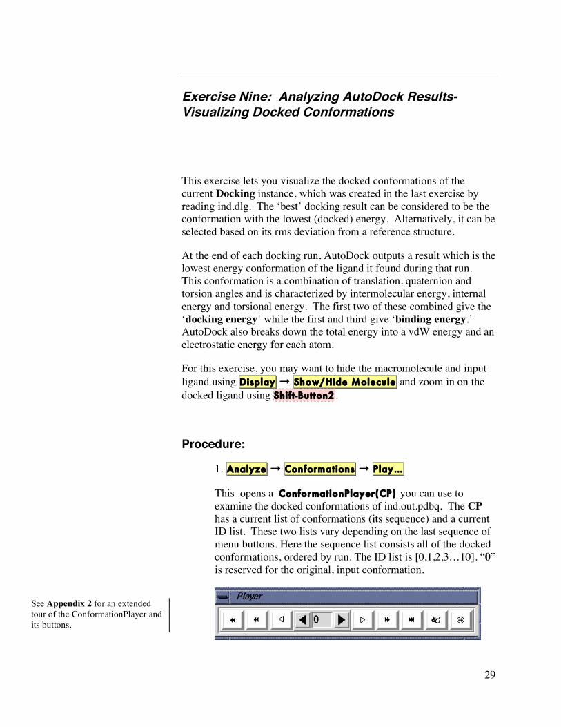
1. Analyze ➞ Conformations ➞ Play…

This opens a ConformationPlayer(CP) you can use to examine the docked conformations of ind.out.pdbq. The CP has a current list of conformations (its sequence) and a current ID list. These two lists vary depending on the last sequence of menu buttons. Here the sequence list consists all of the docked conformations, ordered by run. The ID list is [0,1,2,3…10]. “0” is reserved for the original, input conformation.

See Appendix 2 for an extended tour of the ConformationPlayer and its buttons.

30

• Type-in entry at center for random access to any conformation by its id. Valid ids depend on which menubutton was last used to start the player.

• Click on black arrow buttons next to entry to change to next or previous conformation in current list.

• White arrow buttons start play according to current play mode parameters (see below). Clicking on an active white arrow button stops play. [While a play button is active, its icon is changed to double vertical bars.]

• Double black arrow buttons start play as fast as possible in the specified direction.

• Double black arrow plus l ine buttons advance to beginning or end of conformation list.

• Ampersand button opens the Set Play Options widget (see Appendix 2).

• Quatrefoil button closes the player.

Step through the sequence of conformations one by one using the black arrows. Open the Set Play Options widget by clicking on the Ampersand button. Set the conformation to 4. Change the coloring scheme to vdw or elect_stat in the dropdown menu labelled Color by.

Set the Play Mode to continuously in 1 direction from the Play Mode menu. Click on the forward white arrow. Click again to stop play. Open the Play Parameters widget and set the start frame to 1. This excludes the input conformation which is always conformation 0. Adjust the frame rate to 3. Display information about each conformation by opening the Conformation Info widget by clicking on Show Info.

In the next exercise, we will use the Build button to add new molecules to the Viewer.

31

Exercise Ten: Analyzing AutoDock Results -Clustering Conformations

An AutoDock docking experiment usually has several solutions. The reliability of a docking result depends on the similarity of its final docked conformations. One way to measure the reliability of a result is to compare the rmsd of the lowest energy conformations and their rmsd to one another, to group them into families of similar conformations or “clusters.”

The dpf keyword, analysis, determines whether clustering is done by AutoDock. As you will see below, it is also possible to cluster conformations with ADT. By default, AutoDock clusters docked results at 0.5Å rmsd. This process involves ordering all of the conformations by docked energy, from lowest to highest. The lowest energy conformation is used as the seed for the first cluster. Next, the second conformation is compared to the first. If it is within the rmsd tolerance, it is added to the first cluster. If not, it becomes the first member of a new cluster. This process is repeated with the rest of the docked results, grouping them into families of similar conformations.

First we will examine the AutoDock clustering that we read in from ind.dlg. Next we will make new clusterings at different rms values.

Procedure:

1. Analyze ➞ Clusterings ➞ Show…

Opens an instance of a Python object, an interactive histogram chart labelled ‘ind_out_1:rms = 0.5 clustering’. This chart has bars which represent the clusters computed at the specified rmsd. The bars are sorted by energy of the lowest-energy conformation in that cluster and start off colored blue.

For example, the lowest energy conformation in the second bar is 2_1. The height of the bar represents how many conformations are in that cluster. Clicking on a bar makes that cluster the current sequence for the ligand’s CP, and its color changes to red.

Note: If you have read in more than one docking log into the current Docking or if the results did not

include clustering, you must Recluster… to create a clustering

before you can show one.

Note: lower energies are “better” and in the genetic

algorithm, “fitter.”

Note: if clusterings were performed using several different rms tolerance values, the menu option: Analyze ➞Clusterings➞Show… would open a widget containing a list of the available rms values. Be sure to click only once and to click delicately on this list to open a new interactive histogram. (Otherwise, you may get several identical windows.)

32

The Conformation # Info Widget shows you both refRMSD, the rmsd between the current reference and the displayed conformation and clRMSD, the rmsd between the displayed conformation and the lowest energy conformation in this cluster. As described above in the tour of the CP, you can set the reference coordinates to that of any of the docked conformations when it is the current conformation. When viewing clustering results, this is especially useful because it allows you to examine the rmsd between cluster members. To do this, choose a cluster and use the arrow key to step forward to its lowest energy conformation, e.g. 1-1. Set the rms reference to this conformation. Now, stepping through the cluster will show you the rms difference between the lowest energy member of this cluster, i.e. 1-1, and the rest of the conformations in this cluster.

You can change clusters by picking a different bar in the interactive histogram chart. You can save this histogram as a PostScript file: from the interactive histogram’s menu select Edit ➞ Write to open a file browser for you to enter a filename. Make sure to use “.ps” extension. Select File ➞ Exit to close.

The active-site of the hiv protease has C2 symmetry. You can probably see evidence of this by examining the clusters of docked indinavir molecules.* Step 1 is to build a copy of the lowest energy conformation: cluster 1, conformation 1. First display it via the CP, then click the Build button. Try clicking on the second bar in the histogram and display the lowest energy member of the second cluster by using the arrow keys next to the entry. If this result doesn’t show C2 symmetry, try another cluster bar. You should see the symmetry related docked conformations.

2. Analyze ➞ Clusterings ➞ Recluster…

Opens a widget which lets you enter a series of new rms tolerances as floating point number separated by spaces. These will be used to perform new clustering operations on the docked results. The time consuming step in clustering is computing a difference matrix between conformations to be compared. Larger rms

* Note: To facilitate comparing the docked conformations, type File ➞Preferences➞Set Commands to be Applied on Object s then select colorByMolecules When this is on, each time a new molecule is added to the viewer (up to a current limit of 20), it is colored differently.

33

values require fewer comparisons; conformations which are more similar require fewer comparisons. If you type a name in the OutputfileName: entry, a clustering output file will be written. Our convention is to use the extension “.clust” for these files.

It is important to set the ligand to the original, input conformation (numbered 0) before clustering.

Type in a list of RMSD tolerances separated by spaces thus 1.0 2.0 3.0 and click on OK . For our example, this should be very fast. You can visualize the new clusterings by repeating Step 1.

34

Two Step QA Analysis of AutoDock Results

For quality assurance, after you have read in the docking log(s)

1. Evaluate convergence to determine the thoroughness of the search:

Analyze ➞ Clusterings ➞ Show…

The basic premise is that if you use a large enough number of evaluations, the results will cluster. That is, that there is a small number of ‘best’ results which will be found if you look ‘long enough’. The question you are answering here is ‘were the conditions of the docking experiment sufficient to find these results?’ If the results do not show reasonable clustering, you may want to repeat the docking calculation after increasing the number of evaluations, ga_num_evals, in the dpf. When docking ligands with more than 8-10 active torsions, you will probably need to increase the number of evaluations by a factor of ten or more.

2. Evaluate the chemical reasonableness of the best results by examining the interactions between the receptor and the best docked conformation(s).

Click on the lowest energy cluster in the clustering shown in step one. Put the ligand in the lowest energy conformation using the ConformationPlayer.

Analyze ➞ Macromolecule ➞ Choose…

Look at the interactions between the ligand and nearby atoms in the receptor:

• Is the ligand bound inside a pocket in the receptor? • Are non-polar atoms in the ligand docked near non-polar

atoms in the receptor? Are polar atoms in the ligand docked near polar atoms in the receptor?

• If you know that a particular residue or residues in the protein interact with the ligand, is that interaction shown in the docked result?

Note: In the pharmaceutical industry, medicinal chemists may visually inspect hundreds of docked structures for chemical reasonableness during the drug discovery process.

35

• Do the interactions seem reasonable in the context of what you know about your ligand-receptor from other experimental results such as mutation studies?

The interpretation of AutoDock results is open-ended. In large part it depends on your chemical insight and creativity. Docked poses of the ligand may suggest chemical modifications such as side-group substitutions, etc….

36

Exercise Eleven: Analyzing AutoDock Results-Visualizing Conformations in Context

Ultimately, the goal of a docking experiment is to illustrate the docked result in the context of the macromolecule, explaining the docking in terms of the overall energy landscape. The interactions between the ligand and the macromolecule are driven by energy composed of van der Waals (vdW), electrostatic, hydrogen bonding and desolvation component energies.

This exercise has three parts:

First to evaluate the chemical reasonableness of our results, we will represent the macromolecule as a solvent-excluded surface using msms and check whether the ligand has docked in a ‘pocket’ on the receptor and whether the pairwise-interactions between atoms in the ligand and those in the receptor are reasonable.

Next we will explore the energy landscape of the binding site, representing it using isocontours. This view of the docking can suggest elucidate the binding mechanism and suggest chemical modifications of the ligand.

Finally, we will introduce two ways of visualizing all the docked structures at once, the ‘overall’ binding pattern.

If hsg1 is still in your viewer, skip Step 1. Instead use Display ➞ Show/Hide Molecule to display it. Put indinavir into the lowest energy conformation, 1_1. Also, undisplay any docked conformations you may have already built.

Procedure:

1. Analyze ➞ Macromolecule ➞ Choose…

to link hsg1 to the current docking. If hsg1 is not currently displayed, use Display ➞ Show/Hide Molecule to redisplay it.

37

If hsg1 is not present in your viewer, instead use Analyze ➞ Macromolecule ➞ Open… If hsg1.pdbqs cannot found in the current directory, a file browser open to ask you to specify where it can be found.

2. Select ➞ Direct Select

Opens a Direct Select widget which lets you pick a molecule or chain or named saved set. Click on Molecule List … to display checkbuttons for hsg1 and ind_out . Click on hsg1 . Click on Dismiss to close the widget.

3. Compute ➞ Molecular Surface ➞ Compute Molecular Surface

Opens a MSMS Parameters Panel: widget which lets you set the probe radius and density parameters for the msms surface computation. The density parameter governs the fineness of the calculated mesh. Increase the Density to 10. Click on OK to start the computation.

4. Color ➞ by Atom Type

Click on MSMS-MOL and then click OK . The msms surface will be colored according to the element of the nearest atom.

This view of the docking allows you to see how the docked ligand ‘fits’ into the macromolecule. Verify that polar oxygens and hydrogens are docked near polar atoms in hsg1 and that non-polar carbons are docked near carbons.

Use Un/Display ➞ Molecular Surface to hide the msms surface. You must click on the name of the surface MSMS-MOL as well as the buttons undisplay and OK .

Alternatively, you may want to visualize the docked conformations in the context of the energy grids. This may be useful for computer-aided drug design. In the steps which follow, you will visualize the oxygen affinity map as an isocontour, then display only two residues in the active site of hsg1 and finally see atom O2 of indinavir sitting in a pocket of oxygen affinity between the two ASP25 residues. This is our most complicated exercise.

5. Analyze ➞ Grids ➞ Open…

Note: If you wanted to examine the msms of the various docked

conformations, you could use the CP to step through all the docked

conformations or the conformations in a specific cluster. For each

conformation, you could build a molecule, select that new molecule and

compute an msms surface for it. Display ➞ Show/Hide

molecule turns on and off all the geometries for each molecule.

38

This opens a list chooser of the grids used in this docking. Select hsg1.O.map .

The AutoGrid map file is read into the viewer, creating an instance of a Grid. This map is visualized as an isocontour in 3D. This means that every point in the grid box that is equal to the isocontour level will be connected together by lines or polygons. You can change the isocontour level, which is an energy in Kcal/mol; the step between grid points for sampling the grid values; and whether to show the isocontoured regions as lines or filled (solid) polygons. You can also toggle the visibility of the Grid and its bounding box.

To illustrate the kind of information you can obtain from the atomic affinity grid maps, try this:

1. Set the IsoValue to –0.15 ; if you type into the slider entry, remember to press <Return> or <Enter>.

2. Set the Sampling to 1 and press <Return> or <Enter>.

3. Display hsg1.pdbqs ; if it is not present in the viewer, use Analyze ➞ Macromolecule ➞ Open… .

4. Choose Select ➞ Select From String and type in ASP25 into the Residue field and then click Add . Click Yes to change selection level if necessary and Dismiss to close Select From String widget.

5. Choose Display ➞ Sticks And Balls

Opens Display Sticks and Balls: widget. Increase the quality to 15 and click ok.

Choose Color ➞ By Atom Type and select ‘balls’ and ‘sticks’ in the widget which opens and click OK .

6. Choose a low-energy docked conformation using the CP.

Now you can rotate the objects in the viewer. You will see that the single selected atom in the inhibitor IND201:O2, is buried in a pocket of Oxygen-affinity. If you Build (see below) other low-energy docked conformations, you should be able to see the same O2 atom sitting in this region.

Note: The grid isocontours are colored by atom type. (See

Exercise One for a list of these colors.)

39

Click Display Map and Show Box to undisplay the isocontour and its bounding box before you Dismiss this panel.

It is maybe useful to visualize all the docked conformations at once by placing spheres, one for each docking, at the center of each docked conformation. Here the average of the coordinates is used.

6. Analyze ➞ Dockings ➞ Show as Spheres…

This command represents each docked conformation by a sphere. A sphere is placed at the average position of the coordinates of all the atoms in each conformation. Clicking on the name of a docking log in the list makes the spheres representing its results visible only if the associated ligand is visible.

Click on ind.dlg in the list. You can change the radii of the spheres, their color and their smoothness (or “quali ty ”). [You may need to reduce the radii to .03 to see the overlapping dockings of our result.]

This command gives you a nice overview of the distribution of the docked results.

Finally we will visualize the docked results by building all the conformations. To help distinguish them, first set a user preference to color each added molecule by Molecule. Click on File➞>Preferences➞ Set Commands to be Applied on Objects . Select Color by Molecules . Click on >> and OK .

7. CP ➞ ➞ Build All

This builds a new molecule for each docked conformation in the current set bound to the CP. This gives you a quick idea of the overall results of your docking experiment.

Scripps Research Insti tu te Tutorials Only

If time permits, read in all the results from,/home/user1/results using Analyze->Dockings-> Open All…

Click on Yes when asked Should all the Docking logfiles be read into one Docking?

Recluster using Analyze->Clusterings->Recluster… Click on OK in Clueter ind_out Conformation widget.

Show the Clustering via Analyze->Clustering->Show… Select 2.000 in the Select RMS Tolerance list.

It is expected that there would be only two energy bins in the histogram at this RMS value.

Click on lowest energy bin to open CP. Play all the conformations.

40

Files for exercises:

Input Files: hsg1.pdb ind.pdb

Results Files

Ligand

ind.out.pdbq (6 torsions moving fewest atoms)

Macromolecule

hsg1.pdbqs

AutoGrid

hsg1.gpf hsg1.glg hsg1.*.map hsg1.maps.fld,hsg1.maps.xyz

AutoDock

hsg1.dpf ind.dlg

Useful Scripts extract.py (file.dlg out - pares down dlg) extractDir.py (for all dlgs in this dir) submit.py (launch many dockings on a queue) recluster.py (cluster dlgs)

Customization Options for ADT adt_automergeNPHS: default is 1 adt_autoCtoA: default is 1 adt_editHISprotonation: default is ‘No Change’ autotors_userProteinAromaticList

41

Appendix 1: Docking Parameters

Parameters common to SA, GA, GALS:

'seed': The number of arguments following this keyword determines which random number generator is to be used. One argument causes AutoDock to use the system’s implementation of the random number generator and a corresponding system seed call. One argument is required for the simulated annealing algorithm. Two arguments tells AutoDock to use the platform-independent library for random number generation. Two arguments are required for the genetic algorithm. The arguments themselves can be any combination of explicit long integers, the key word ‘time’ or the keyword ‘pid’. ‘time’ is the number of seconds since the epoch, referenced to 00:00:00CUT 1 Jan 1970. ‘pid’ gives the UNIX process ID of the currently executing AutoDock process.

'types': Atom names for all atom types present in ligand.

'fld': grid data field file created by AutoGrid and readable by AVS.

'map': filename for the first AutoGrid affinity grid map of the 1st atom type. Repeated for all atom types specified in ‘types’ plus ‘e’ for required electrostatics map.

'move': filename for the ligand to be docked.

'about': x y z center of ligand about which rotations will be made. Coordinate frame of reference inside AutoDock. That is, internally the ligand’s coordinates become centered at the origin.

'tran0': initial coordinates for the center of the ligand or random. Each new run starts the ligand from this location. Please note: the user should enscure that the ligand, when translated to these coordinates still fits inside the volume of the grid maps. If there are some atoms which do lie outside this volume, AutoDock will automatically move the ligand until the ligand is completely inside the box.

'quat0': initial quaternion Qx, Qy, Qz, Qw or random.

'ndihe': number of rotatable bonds in the ligand.

42

'dihe0': initial relative dihedral angles or random. There must be ndihe number of values specified if the user decides to explicitly set the initial relative dihedrals.

'tstep': if one argument, the maximum translation jump per step. If single argument and less than one, the reduction factor is multiplied with the tstep at the end of each cycle to get next value. Alternatively, if there are two arguments, the user specifies the value for the first and last cycle and AutoDock calculates the reduction factor that satisfies these constraints. Default is 2.0 Angstrom

'qstep': maximum orientation step size for the angular component w of quaternion. Default is 50.0 degrees.

'dstep': maximum dihedral step size. Default is 50.0 degrees.

'torsdof': number and coefficient of the torsional degrees of freedom for the estimation of the change of free energy upon binding. Here, the number of possible rotatable bonds in the ligand excluding any torsions that only rotate hydrogens: eg hydroxyls, amines… The coefficient is 0.3113 kcal/mol

'intnbp_r_eps': internal pairwise non-bonded energy parameters for the flexible ligand: equilibrium distance and well depth followed by integer exponents n and m.

'intelec': Optional: whether to calculate internal ligand electrostatic energies. Default is no.

'outlev': diagnostic output level. For simulated annealing 0= no output, 1=minimal output, 2 = full state output at end of each cycle, 3=detailed output for each step. For GA and GA-LS: 0=minimal output, 1= write minimum, mean and maximum of each state variable at the end of every generation. Use outlev 1 for SA and outlev 0 for GA and GA-LS.

'rmstol': the rms deviation tolerance for cluster analysis, carried out after multiple docking runs. If two conformations have an rms less than this tolerance, they will be placed in the same cluster. The structures are ranked by energy, as are the clusters.

'rmsref': the root mean square deviation of the docked conformations calculated with respect to the coordinates in the pdbq file or pdb file specified here. Particularly useful for comparing a docked result to a known crystal structure.

43

'extnrg': external grid energy assigned to any atoms that stray outside the volume of the grid during a docking. Default is 1000. kcal/mole.

'analysis': perform a cluster analysis on results of a docking and output results to the log file. The docked conformations are sorted in order of increasing energy, then compared by root mean square deviation. If the docked result is within the ‘rmstol’ threshold, it is placed into the same cluster.

Simulated Annealing Specific Parameters:

'rt0': initial annealing temperature-actually absolute temperature multiplied by the gas constant. Default is 500. cal/mole.

'e0max': two floats-used only in SA. Keyword stipulates that the ligand’s initial state cannot have an energy greater than the first value, nor can there be more than the second value’s number of retries. Default is 0, 10000.

'linear_schedule': instructs AutoDock to use a linear temperature reduction schedule during Monte Carlo simulated annealing. Unless given, a geometric reduction schedule is used according to rtrf described below. Default is to use linear_schedule.

'rtrf': annealing temperature reduction factor. At the end of each cycle the annealing temperature is multiplied by this factor to give that of the next cycle. Must be positive and less than one. Default is 0.95

'trnrf': per cycle reduction factor for translations. Default is 1.0.

'quarf': per cycle reduction factor for quaternions. Default is 1.0.

'dihrf': per cycle reduction factor for dihedrals. Default is 1.0

'runs': number of automated docking runs to carry out. Default is 10.

'cycles': number of temperature reduction cycles. Default is 50.

'accs': Maximum number of accepted steps per cycle. Default is 100.

'rejs': Maximum number of rejected steps per cycle. Default is 100.

44

'select': State selection flag. ‘m’ minimum state is selected or ‘l’ last state. Default is m.

'simanneal': instructs AutoDock to do specified number of docking runs using the simulated annealing SA search engine.

Genetic Algorithm Specific Parameters:

'ga_pop_size': number of individuals in the population. Each individual is a coupling of a genotype and its associated phenotype. Typical values range from 50 to 200. Default is 50.

'ga_num_evals':Maximum number of energy evaluations that a GA run should make. Default is 250000.

'ga_num_generations': Maximum number of generations that a GA or LGA run should last. Default is 27000.

'ga_elitism': Number of top individuals that are guaranteed to survive into the next generation. Default is 1.

'ga_mutation_rate': The probability that a particular gene is mutated. Default is 0.02

'ga_crossover_rate': Crossover rate is the expected number of pairs in the population that will exchange genetic material. Setting this value to 0 turns the GA into the evolutionary programming method (EP) but that requires a concomitant increase in the ga_mutation_rate in order to be effective. Default is 0.80.

'ga_window_size': Number of preceding generations to take into consideration when deciding the threshold for the worst individual in the current population. Default is 10.

'ga_cauchy_alpha': Alpha parameter in a Cauchy distribution which corresponds roughly to the mean of the distribution. Default is 0.

'ga_cauchy_beta': Beta parameter in a Cauchy distribution which corresponds roughly to something like the variance of the distribution. However, the Cauchy distribution doesn’t have finite variance. Default is 1.

45

'set_ga': sets the global optimizer to be a genetic algorithm. PLEASE note all ga_ parameters must be specified before this line in order to be used in the docking.

'do_global_only': instructs AutoDock to carry out docking using only a global search. Local search parameters in the dpf are ignored when this is present.

Local Search Specific Parameters:

'sw_max_its': Maximum number of iterations that the local search procedure applies to the phenotype of any given individual. Default is 50.

'sw_max_succ': Number of successes in a row before a change is made to the rho parameter in Solis & Wets algorithm. Default is 4.

'sw_max_fail': Number of failures in a row before Solis & Wets algorithms adjust rho. Default is 4.

'sw_rho': Parameter defining the initial variance and specifying the size of the local space to sample. Default is 1.0.

'sw_lb_rho': Lower bound on rho, the variance for making changes to genes. Rho can never be modified to a value smaller than sw_lb_rho. Default is 0.01.

'ls_search_freq': The probability of any particular phenotype being subjected to local search. Default is 0.06.

'set_psw1': Instructs AutoDock to use the pseudo-Solis and Wets local searcher. This method maintains the relative proportions of variances for the translations in Angstrom and the rotations in radians. These are typically 0.2 Angstrom and 0.087 radians to start with so the variance for translations will always be 2.3 times larger than that for the rotations (i.e. the orientation and torsions).

'do_local_only': Instructs AutoDock to carry out only the local search of a global-local search. The genetic algorithm parameters are ignored, except for the population size. This is an ideal way of carrying out a minimization using the same force field as is used during the dockings. The ga_run keyword should not be given. The integer following the keyword determines how many dockings will be performed. Default is 50.

46

GALS parameters include all Genetic Algorithm and Local Search parameters listed above except do_global_only and do_local_only.

Clustering keywords:

'cluster': keyword specific to reclustering jobs. Parameter which follows is filename for concatenated docking logs. Script ‘recluster.py’ produces this kind of file.

'rmstol': root mean square tolerance for reclustering.

'types': types of atoms present in ligand

'write_all_cluster_members': option causes printed output of all docked structures in each cluster. Default is to write the first docked structure in each cluster only. (The first docked structure has the lowest energy of all the docked structures in the cluster.)

47

Appendix 2: Conformation Player

• Type-in entry at center for random access to any conformation by its id. Valid ids depend on which menubutton was last used to start the player.

• Click on black arrow buttons next to entry to change to next or previous conformation in current list.

• White arrow buttons start play according to current play mode parameters (see below). Clicking on an active white arrow button stops play. [While a play button is active, its icon is changed to double vertical bars.]

• Double black arrow buttons start play as fast as possible in the specified direction.

• Double black arrow plus l ine buttons advance to beginning or end of conformation list.

• Ampersand button opens the Set Play Options widget (see next).

• Quatrefoil button closes the player.

Next, a tour of the Set Play Options widget and its buttons:

48

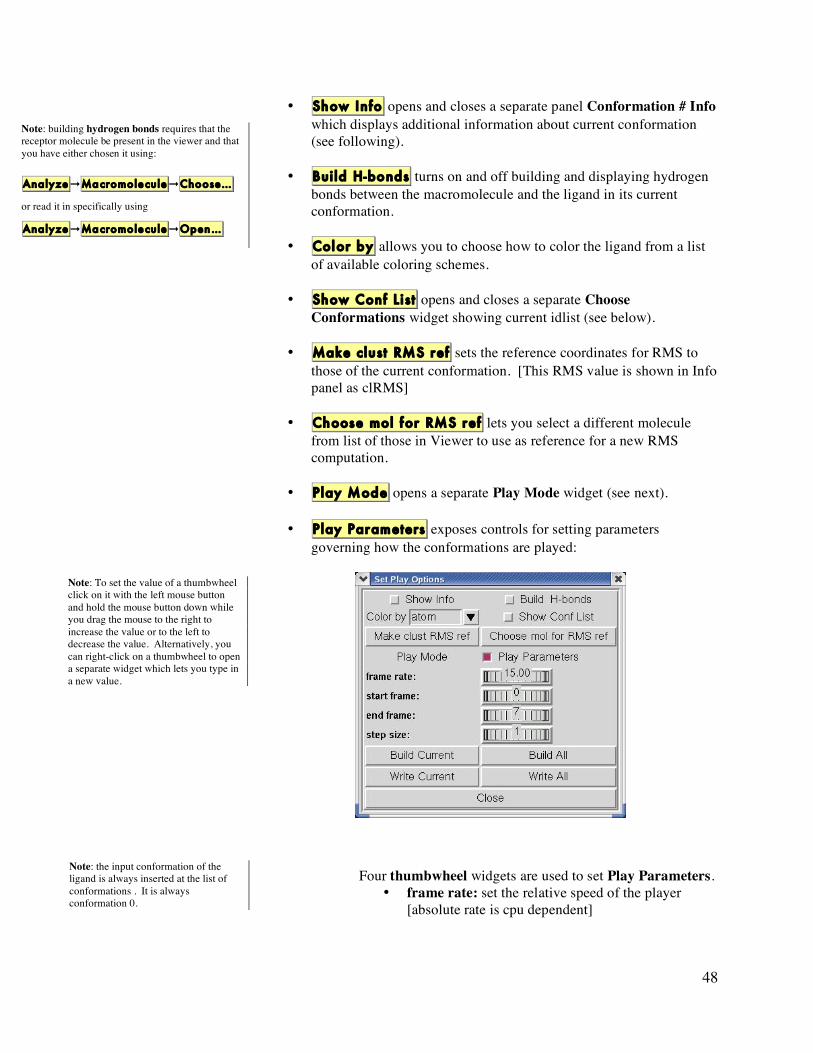
• Show Info opens and closes a separate panel Conformation # Info which displays additional information about current conformation (see following).

• Build H-bonds turns on and off building and displaying hydrogen bonds between the macromolecule and the ligand in its current conformation.

• Color by allows you to choose how to color the ligand from a list of available coloring schemes.

• Show Conf Li st opens and closes a separate Choose Conformations widget showing current idlist (see below).

• Make clust RMS ref sets the reference coordinates for RMS to those of the current conformation. [This RMS value is shown in Info panel as clRMS]

• Choose mol for RMS ref lets you select a different molecule from list of those in Viewer to use as reference for a new RMS computation.

• Play Mode opens a separate Play Mode widget (see next).

• Play Parameters exposes controls for setting parameters governing how the conformations are played:

Four thumbwheel widgets are used to set Play Parameters. • frame rate: set the relative speed of the player

[absolute rate is cpu dependent]

Note: To set the value of a thumbwheel click on it with the left mouse button and hold the mouse button down while you drag the mouse to the right to increase the value or to the left to decrease the value. Alternatively, you can right-click on a thumbwheel to open a separate widget which lets you type in a new value.

Note: the input conformation of the ligand is always inserted at the list of conformations . It is always conformation 0.

Note: building hydrogen bonds requires that the receptor molecule be present in the viewer and that you have either chosen it using:

Analyze ➞Macromolecule ➞Choose…

or read it in specifically using

Analyze ➞Macromolecule ➞Open…

49

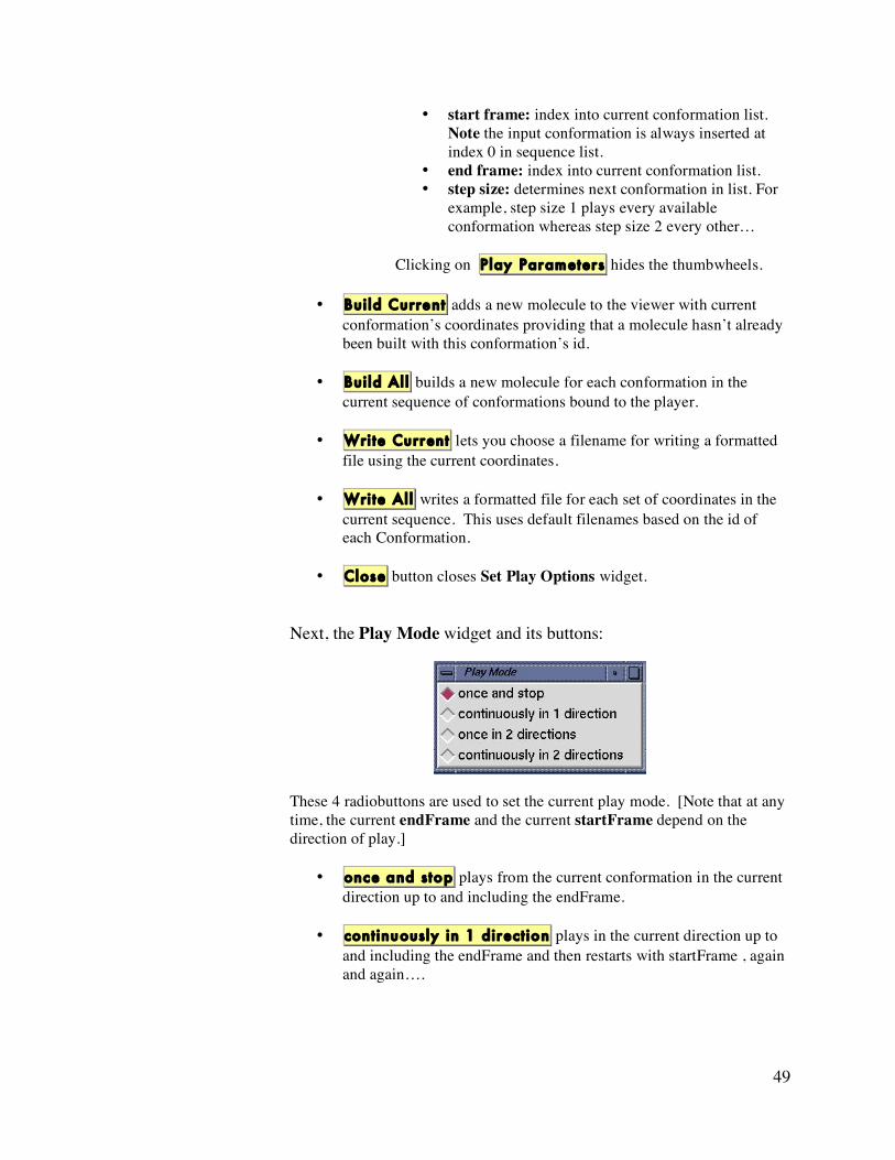
• start frame: index into current conformation list. Note the input conformation is always inserted at index 0 in sequence list.

• end frame: index into current conformation list. • step size: determines next conformation in list. For

example, step size 1 plays every available conformation whereas step size 2 every other…

Clicking on Play Parameters hides the thumbwheels.

• Build Current adds a new molecule to the viewer with current conformation’s coordinates providing that a molecule hasn’t already been built with this conformation’s id.

• Build All builds a new molecule for each conformation in the current sequence of conformations bound to the player.

• Write Current lets you choose a filename for writing a formatted file using the current coordinates.

• Write All writes a formatted file for each set of coordinates in the current sequence. This uses default filenames based on the id of each Conformation.

• Close button closes Set Play Options widget.

Next, the Play Mode widget and its buttons:

These 4 radiobuttons are used to set the current play mode. [Note that at any time, the current endFrame and the current startFrame depend on the direction of play.]

• once and stop plays from the current conformation in the current direction up to and including the endFrame.

• continuously in 1 direction plays in the current direction up to and including the endFrame and then restarts with startFrame , again and again….

50

• once in 2 directions plays from the current conformation in the current direction up to and including the endFrame and then plays back to startFrame and stops.

• continuously in 2 directions plays from current conformation in current direction up to endFrame then back to the beginning then back to the end, again and again….

•

The Choose Conformation widget:

Choose Conformation widget has list of ids for each conformation in the current sequence list. Double clicking on an entry in this list updates the ligand to the corresponding conformation. This widget is closed by clicking on the checkbutton Show Conf List in Set Play Options widget.

Conformation # Info widget shows information about a specific conformation from a docking experiment.

• binding energy is the sum of the intermolecular energy and the torsional free-energy penalty.

• docking energy is the sum of the intermolecular energy and the ligand’s internal energy.

51

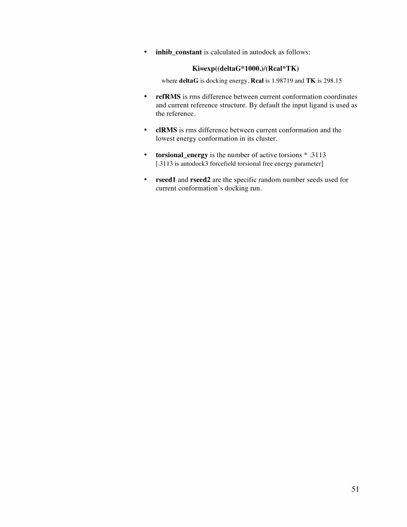
• inhib_constant is calculated in autodock as follows:

Ki=exp((deltaG*1000.)/(Rcal*TK) where deltaG is docking energy, Rcal is 1.98719 and TK is 298.15

• refRMS is rms difference between current conformation coordinates and current reference structure. By default the input ligand is used as the reference.

• clRMS is rms difference between current conformation and the lowest energy conformation in its cluster.

• torsional_energy is the number of active torsions * .3113 [.3113 is autodock3 forcefield torsional free energy parameter]

• rseed1 and rseed2 are the specific random number seeds used for current conformation’s docking run.