adult owveld largescale yellowfish abeobarbusmjejane game reserve, especially j. bardenhorst who...

i

CHARACTERISATION OF THE HEALTH, HABITAT USE AND MOVEMENT OF

ADULT LOWVELD LARGESCALE YELLOWFISH (LABEOBARBUS

MAREQUENSIS SMITH, 1841) AND OTHER FISHES IN THE CROCODILE

RIVER, KRUGER NATIONAL PARK.

By

MATTHEW JAMES BURNETT

A Thesis submitted in fulfilment of the requirements for the Degree

MASTERS OF SCIENCE

In

AQUATIC HEALTH

IN THE DEPARTMENT OF ZOOLOGY, FACULTY OF SCIENCE

AT THE

UNIVERSITY OF JOHANNESBURG

Supervisor: PROFESSOR VICTOR WEPENER (UNIVERSITY OF JOHANNESBURG)

MAY 2013

ii

Thanks to God

"But ask the animals, and they will teach you, or the birds of the air, and they

will tell you; or speak to the earth, and it will teach you, or let the fish of the

sea inform you. Which of all these does not know that the hand of the LORD

has done this? In his hand is the life of every creature and the breath of all

mankind.”

Job 12:7-10

iii

TABLE OF CONTENTS

ACKNOWLEDGMENTS………………………………………………………………….....V

SUMMARY…………………………………………………………………………………..VI

LIST OF TABLE……………………………………………………………………………..IX

LIST OF FIGURES………………………………………………………………………….IX

LIST OF APPENDICES……………………………………………………………………XII

1 CHAPTER 1: INTRODUCTION AND PROBLEM FORMULATION. ................... 1

1.1 Study Area ................................................................................................. 6

2 CHAPTER 2: A COMPREHENSIVE LITERATURE REVIEW ON LOWVELD

LARGESCALE YELLOWFISH, LABEOBARBUS MAREQUENSIS ........................... 8

2.1 Introduction ................................................................................................ 8

2.2 Labeobarbus marequensis past and present ............................................. 9

2.3 Labeobarbus marequensis biology and ecology ...................................... 11

2.4 Labeobarbus marequensis ecosystem service use .................................. 15

3 CHAPTER 3: BEHAVIOURAL STUDY OF AN ADULT POPULATION OF

LOWVELD LARGESCALE YELLOWFISH (LABEOBARBUS MAREQUENSIS) IN

THE CROCODILE RIVER, KRUGER NATIONAL PARK. ........................................ 17

3.1 Introduction .............................................................................................. 17

3.2 Material and Methods .............................................................................. 18

3.2.1 Biotelemetry systems ............................................................................... 18

3.2.2 Capture and tagging ................................................................................ 22

3.2.3 Monitoring techiniques ............................................................................. 27

3.2.4 Habitat preferences .................................................................................. 29

3.2.5 Behavioural variables ............................................................................... 30

3.2.6 Data analysis ........................................................................................... 31

3.3 Results ..................................................................................................... 31

3.3.1 Habitat Preference ................................................................................... 32

3.3.2 Behaviour variables ................................................................................. 42

3.4 Discussion ............................................................................................... 45

3.4.1 Habitat preferences .................................................................................. 45

3.4.2 Behaviour variables ................................................................................. 46

3.5 Conclusion ............................................................................................... 48

4 CHAPTER 4: METAL BIOACCUMULATION IN LOWVELD LARGESCALE

YELLOWFISH (LABEOBARBUS MAREQUENSIS), TIGERFISH (HYDROCYNUS

VITTATUS) AND SHARPTOOTH CATFISH (CLARIAS GARIEPINUS) FROM THE

CROCODILE AND SABIE RIVERS, KRUGER NATIONAL PARK. .......................... 50

iv

4.1 Introduction .............................................................................................. 50

4.2 Materials and Methods ............................................................................. 52

4.3 Results ..................................................................................................... 53

4.4 Discussion ............................................................................................... 63

4.5 Conclusion ............................................................................................... 65

5 CHAPTER 5: GENERAL CONCLUSION AND MANAGEMENT

RECOMMENDATIONS. .......................................................................................... 67

5.1 General conclusions ................................................................................ 67

5.2 Management recommendations ............................................................... 68

6 CHAPTER 6: REFERENCES .......................................................................... 70

7 CHAPTER 7: APPENDICES ............................................................................ 80

v

ACKNOWLEDGMENTS

Special Thanks and appreciation to the following people and organisations

My God and saviour Jesus Christ, who created all things and has given

me the opportunity and ability to achieve all I have.

Gordon O’Brien, for his support, expertise, assistance and his effort

into helping me make this thesis a success.

My Supervisor, Professor Victor Wepener for his professional

assistance and expertise.

My loving parents whom without their moral and continual support I

would not have achieved what I have today

Bruce Leslie, for his vision, fishing rod and rifle, without him none of

this would have happened.

The Head of Department in Zoology (University of Johannesburg)

Professor J.H.J. van Vuren for the use of facilities.

The South African National Parks (SANParks), Kruger National Park

personal especially D. Pienaar and A. Deacon for there assistance and

guidance throughout the study.

The Water Research Commission (WRC) for funding the study.

Mjejane Game Reserve, especially J. Bardenhorst who allowed us

access and support during the study.

Wireless Wildlife for their professional assistance in developing tags for

the study.

vi

SUMMARY

Yellowfish and specifically Labeobarbus marequensis are a charismatic species

targeted by anglers throughout South Africa. Their population are limited to the north-

western parts of the country including the lower reaches of the Crocodile River that

flows through the Kruger National Park (KNP). Despite conservation efforts the

Crocodile River in the KNP is still highly impacted. The effect of these impacts on the

ecosystem is largely unknown.

The main aim of the study was to determine the influence of changing water quantity

and quality in the Crocodile River on adult L. marequensis. This was achieved by

evaluating altered flows (discharge) on the behaviour of adult L. marequensis in the

Crocodile River using biotelemetry over a two year period. The influence of altered

water quality was assessed using metal bioaccumulation as an indicator of metal

exposure in L. marequensis, Clarias gariepinus and Hydrocynus vittatus in the

Crocodile and Sabie Rivers during a high and low flow season.

Biotelemetry was used on 16 L. marequensis and 12 H. vittatus to determine the

habitat use and movement responses of the species. Fish were tagged with

Advanced Telemetry Systems (ATS) and Wireless Wildlife (WW) tags and tracked

remotely and manually. Home ranges were determined using Arc GIS ®, Habitat

uses were analyzed using Windows Excel (© 2011, Microsoft inc.). Environment

variables recorded were scored as primary and secondary and then combined with a

weighting variable 2:1 ratio (primary variable: secondary variable). A mixed-model

analysis of variance (ANOVA) approach with a random co-efficients model and

Akaike’s information criteria (AIC) were used to test for significance. Analyses were

conducted using SAS version 9 (SAS institute, Cary, NC).

The habitat use of L. marequensis included cobble and boulder dominated flowing

habitat biotopes. A strong affiliation for cover features including rocky outcrops,

undercut banks and submerged woody and rock structures were also observed.

Foraging behaviour took place predominantly within in these habitat types. A single

spawning event was observed within a fast flowing, boulder dominated and 1-2m

deep run. Seasonal habitat utilization differed significantly (p=0.04). Changes in

discharge significantly (p=0.001) effected behaviour. During high flow periods the

movement of fish decreased. Significant (p=0.05) changes in movement were

observed during rapid moderate (increase of 11m3/s) and high (61 m3/s) changes in

vii

discharge. The study indicates that habitat available for L. marequensis is low within

KNP and the focal area is important to the species. Reduction in habitat diversity

could impact the behaviour of the species. The management of the timing, duration

and frequency of flows are important for the biology and ecology of L. marequensis.

For the metal bioaccumulations L. marequensis, C gariepinus and H. vittatus were

caught in two rivers, the Sabie and Crocodile River during a high flow and low flow

period. In total 19 L. marequensis, 23 C. gariepinus and 30 H. vittatus were used.

The fishes spinal cords were severed and then dissected and muscle tissue removed

and frozen for analysis. Tissue were then dried at 60°C for 48 hours, then after

weighed and diluted in 1% HNO3 (AR) with Milli-Q water before digestion using

HNO3/H2O2 and using an Ethos microwave digestion system. Metal concentrations

were determined using a Thermo inductively coupled plasma optical emission

spectrophotometer (ICP-OES) and an inductively coupled plasma mass

spectrophotometer (ICP-MS). Metals analysed were As, Cd, Cr, Cu, Mn, Ni, Pb, Se

and Zn. Quality control of metal measurements in sediment and muscle tissue was

verified by including process blanks and certified reference material (CRM 278,

muscle tissue Community Bureau of Reference, Geel, Belgium). Statistical analyses

of significant differences, between sites and species were undertaken using one-way

analyses of variance (ANOVA). Data were tested for normality and homogeneity of

variance using Kolmogorov-Smirnov and Levene’s tests (Zar, 1996), respectively,

prior to applying post-hoc comparisons. Post-hoc comparisons were made using the

Scheffe test for homogeneous or Dunnett’s-T3 test for non-homogenous data. The

use of either one of the two tests resulted in the determination of significant

differences (p<0.05) between variables.

The metal bioaccumulations showed to have significant (p<0.05) differences between

the Crocodile River and Sabie River, high flow and low flow and between the three

species. Aluminium, Fe and Se were significantly (p<0.05) higher during the high flow

in the Crocodile River for L. marequensis while Cr, Fe and Se was significantly

(p<0.05) higher during high flows in the Sabie River for L. marequensis. Zinc was

significantly (p<0.05) higher in L. marequensis than in C. gariepinus during Crocodile

River high flows. Arsenic was significantly (p<0.05) higher in L. marequensis than H.

vittatus during the Crocodile River low flows. Within the Sabie River Al and Pb was

significantly (p<0.05) higher in L. marequensis than in C. gariepinus and significantly

(p<0.05) higher in L. marequensis than in H. vittatus respectively during high flows.

During low flows for the Sabie River Mn and Se were significantly (p<0.05) higher in

viii

L. marequensis than in C. gariepinus, Se in L. marequensis was significantly (p<0.05)

higher than in H. vittatus. Differences between the two rivers during high flows

showed significantly (p<0.05) higher levels of Cd in L. marequensis and Co in H.

vittatus in the Crocodile River. During low flow spatial differences between the two

rivers, the Crocodile River showed L. marequensis to have significantly (p<0.05)

higher levels for Al, Cr and Cd bioaccumulation. Cadmium in H. vittatus and As in C.

gariepinus had significantly (p<0.05) higher metal bioaccumulations for the Crocodile

River than in the Sabie River.

The hypothesis set were accepted and able to indicate the importance of flow

(discharge), season and time of day on the behavioural response of L. marequensis

and the importance of maintaining the preferred habitat for the species to ensure its

survival. Discharge in river management is always of importance as it alters

downstream available habitat. Constant flow allows the river to stabilize creating

preferred habitat to be around for longer, this is not to distract from natural flows yet

to enhance natural flows and not allow the release of water at irregular intervals. The

importance of spring flows to L. marequensis behaviour indicates the value of natural

flows during that period to allow for availability of spawning events. Further

minimizing the effluent of metal wastes into the Crocodile River system is also of

importance as metal concentrations were found to be higher within the Crocodile

River than in the Sabie River. Therefore fish in the Crocodile River are potentially at a

greater risk than that in the Sabie River. Thus minimizing or reducing the release of

metals into the Crocodile River would reduce the risks.

Further studies are needed to better understand the spawning habits of L.

marequensis and the associated cues in particular to the day length, flows and

associated spawning habitat. Since L. marequensis bio-accumulated the highest

levels of metals it is recommended that the species be used as an indicator species.

Future studies should be aimed at linking the metal exposure (in the form of

bioaccumulation) with the effects, e.g. using biomarkers of which behaviour could

form a part.

ix

LIST OF TABLES

Table 1: Types of tags used by Advanced Telemetry Systems and Wireless Wildlife

Systems in the study. Wireless Wildlife tags Series V included a LED light and series

IV included a depth sensor. ..................................................................................... 19

Table 2: Species, tag type, capture location, monitoring period from capture date to

the last day monitored (end date) and fixes during manual and remote monitoring

during the study. ...................................................................................................... 26

Table 3: Spatial habitat data associated with the observed locations and movement

of the tagged L. marequensis monitored during the study. ...................................... 30

Table 4: Cover Features and Habitat Biotopes for the key area’s within the Crocodile

Site .......................................................................................................................... 36

LIST OF FIGURES

Figure 1: Shows the location of the Crocodile Site on the Crocodile River and the

control sample sites along the Sabie River, KNP. ...................................................... 7

Figure 2: Distribution range of Labeobarbus marequensis in Africa (after Fouché,

2007). ...................................................................................................................... 11

Figure 3: Picture showing a Labeoabarbus marequensis caught within the lower

reaches of the Crocodile River, Kruger National Park. ............................................. 12

Figure 4: Advanced Telemetry Systems’ tags, models 2030, 2060 (A) and 1930 (H)

used in the study and attached to fish. Hydrocynus vittatus with an ATS 2060b

transmitter (B), Labeobarbus marequensis with an ATS 2030 transmitter (E) and

1930 transmitter (I). Wireless Wildlife Systems’ tags, Series III (D), Series IV (G) and

Series V (K) used in the study attached to Hydrocynus vittatus (C) and Labeobarbus

marequensis (F and J). ........................................................................................... 20

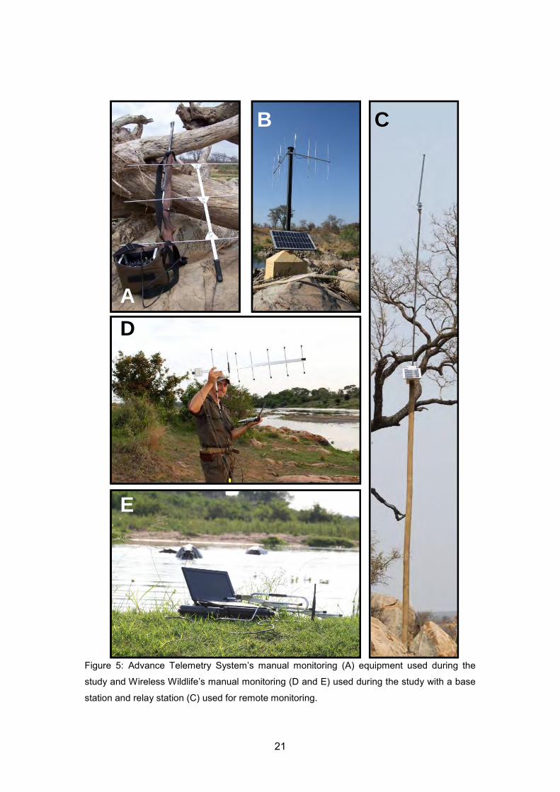
Figure 5: Advance Telemetry System’s manual monitoring (A) equipment used during

the study and Wireless Wildlife’s manual monitoring (D and E) used during the study

with a base station and relay station (C) used for remote monitoring. ...................... 21

Figure 6: Placement of the remote stations used for the Wireless Wildlife system

covering the Crocodile Site. The signal range for each station is indicated by colour,

yellow being the strongest to red being the weakest. ............................................... 22

Figure 7: Capture techniques, Fly fishing (A and G), bait fishing with worms, corn and

crickets (E and F), Netting (D), electro-fisher (220 V) (B) and Casting nets (C) were

used in order to obtain suitable fish for the study. .................................................... 23

Figure 8: The tagging procedures included: capture fish and the equipment needed

to tag the fish (A). The fish is anaesthetised before operating and then submerged

x

back into the water once the spinal needles have been inserted to start recovery (B,

C). The spinal needles are inserted through the muscle below the dorsal fin and anti-

biotics applied into the needles to coat the anchoring wires from the transmitter (D,

E). Plastic and metal sleeves are placed onto the coated anchoring wires and

crimped (F) more anti-biotics are applied around the tag and above the head (G).

Fish measurements are recorded (H) the fish recovery starts (I) and the fish once

fully recovered allowed to swim away freely (J, K). .................................................. 25

Figure 9: Schematic diagram presenting the monitoring methods followed out during

monitoring surveys adopted from O’Brien and De Villiers (2011) ............................. 28

Figure 10: The home ranges of Labeobabrbus marequensis for individuals LMAR 1

(A), LMAR 2 (B) and LMAR 3 (C). ........................................................................... 33


(A), LMAR 5 (B) and LMAR 6 (C). ........................................................................... 34


(A), LMAR 8 (B) and LMAR 9 (C). ........................................................................... 35

Figure 13: Depicts the key sites L. marequensis, with their referenced names, along

the Crocodile River study area. ............................................................................... 36

Figure 14: Pictures depicting the key areas in the Crocodile Site and main habitats

where tagged individuals were found most frequently: Key area 4 (A); A channel (B);

Key area 3 (C); the location where LMAR2, LMAR5, LMAR6 and LMAR9 were

tagged (D and E); Key area 2 (G, H) where LMAR1 was tagged; Key area 1 where

LMAR3 and LMAR4 were tagged and found regularly (F) ....................................... 37

Figure 15: Cover features (A and B) and Biotopes preference of L. marequensis (A

and C) and H. vittatus (B and D). ............................................................................. 38

Figure 16: Discharges (m3.s-1) for the Crocodile River and season correlation for the

duration of the study. ............................................................................................... 39

Figure 17: Cover features (A-D) and Biotopes (E-H) of Labeobarbus marequensis for

different seasons, Summer (A and E), Autumn (B and F), Winter (C and G) and

Spring (D and H). .................................................................................................... 40

Figure 18: Cover features (A-C) and Biotopes (D-F) of Labeobarbus marequensis for

different flows (discharge), low flow (A and D), moderate flow (B and E), high flow (C

and E). .................................................................................................................... 41

Figure 19: The movement (activity counts) (A and B) and depth (mm) (C and D)

relationship between time of day for Labeobarbus marequensis (A and C) and

Hydrocynus vittatus (B and D). ................................................................................ 43

Figure 20: The movement (activity counts) (A) and depth (mm) (B) relationship

between seasons for Labeobarbus marequensis. ................................................... 44

xi

Figure 21: The movement (activity counts) (A) and depth (mm) (B) relationship

between flows (discharges) for Labeobarbus marequensis. .................................... 45

Figure 22: Metal bioaccumulation in muscle tissue (mean standard error in g/g dw)

of Labeobarbus marequensis (nHF=4 & nLF=6), C. gariepinus (nHF =1 & nLF=9) and H.

vittatus (nHF=10 & nLF=3) during the high and low flow sampling surveys in the

Crocodile River. Within surveys, means with common alphabetical superscript

indicate significant differences between species (p<0.05), while asterisks indicate

significant differences between surveys for a particular species. ............................. 55


of Labeobarbus marequensis (nHF=4 & nLF=6), C. gariepinus (nHF =1 & nLF=9) and H.

vittatus (nHF=10 & nLF=3) during the high and low flow sampling surveys in the

Crocodile River. Within surveys, means with common alphabetical superscript

indicate significant differences between species (p<0.05), while asterisks indicate

significant differences between surveys for a particular species. ............................. 56


of Labeobabrbus marequensis (nHF=3 & nLF=6), C. gariepinus (nHF =9 & nLF=4) and H.

vittatus (nHF=8 & nLF=9) during the high and low flow sampling surveys in the Sabie

River. Within surveys, means with common alphabetical superscript indicate

significant differences between species (p<0.05), while asterisks indicate significant

differences between surveys for a particular species. Below detectable limits is

indicated by BDL. .................................................................................................... 57

Figure 25: Metal bioaccumulation in muscle tissue (mean standard error in g/g

dw) of Labeobarbus marequensis (nHF=3 & nLF=6), C. gariepinus (nHF =9 & nLF=4)

and H. vittatus (nHF=8 & nLF=9) during the high and low flow sampling surveys in the

Sabie River. Within surveys, means with common alphabetical superscript indicate


differences between surveys for a particular species. .............................................. 58


of Labeobarbus marequensis (nCR=6 & nSR=6), C. gariepinus (nCR=9 & nSR=4) and H.

vittatus (nCR=3 & nSR=9) between the Crocodile River and Sabie River during low

flows. Within surveys, means with common alphabetical superscript indicate



indicated by BDL. .................................................................................................... 59



vittatus (nCR=3 & nSR=9) between the Crocodile River and Sabie River during low

xii




indicated by BDL. .................................................................................................... 60



vittatus (nCR=10 & nSR=8) between the Crocodile River and Sabie River during high




indicated by BDL. .................................................................................................... 61



vittatus (nCR=10 & nSR=8) between the Crocodile River and Sabie River during high



differences between surveys for a particular species. .............................................. 62

LIST OF APPENDICES

Appendix 1: RAW data acquired during manual monitoring observations ................ 81

Appendix 2: Continuation of RAW data acquired during manual monitoring

observations ............................................................................................................ 82


observations ............................................................................................................ 83


observations ............................................................................................................ 84


observations ............................................................................................................ 85


observations ............................................................................................................ 86


observations ............................................................................................................ 87


observations ............................................................................................................ 88


observations ............................................................................................................ 89

xiii


observations ............................................................................................................ 90

Appendix 11: Graphical representation of the home for the 2.5 kg Labeobarbus

marequensis LMAR1, with ATS tag 2030 frequency 142.214. Tagged on the

15/08/2009 and monitored until the 19/09/2009, monitored on 15 occasions. .......... 91












16/08/2009 and monitored until the 17/02/2011, monitored on 109 occasions. ........ 95




Appendix 17: Graphical representation of the home for the 3 kg Labeobarbus






Appendix 19: Graphical representation of the home for the 2.6 kg Labeobarbus.



Appendix 20: Graphical depiction of: The 2.5 kg Labeobarbus marequensis LMAR10,

with WW tag Series IV no. 6, tagged on the 19/09/2011, tag active until the

01/06/2012 (A). The 2.8 kg L. marequensis LMAR11, with WW tag Series III no. 25,

tagged on the 19/09/2011, tag active until the 01/06/2012 (B). The 2.5 kg L.

marequensis LMAR12, with WW tag Series IV no. 7, tagged on the 19/09/2011, tag

active until the 01/06/2012 (C). The 2.3 kg L. marequensis LMAR13, with WW tag

Series III no. 17, tagged on the 19/09/2011, tag active until the 01/06/2012 (D). The

2.2 kg L. marequensis LMAR14, with WW tag Series III no. 12, tagged on the

xiv

19/09/2011, tag active until the 01/06/2012 (E). The 2.3 kg L. marequensis LMAR15,

with WW tag Series III no. 14, tagged on the 15/10/2011, tag active until the

01/06/2012 (F). The 3.9 kg L. marequensis LMAR16, with WW tag Series III no. 42,

tagged on the 29/11//2011, active until the 01/06/2012 (G). .................................. 100

Appendix 21: Graphical depiction of: The 1.3 kg Hydrocynus vittatus HVIT1, with ATS

tag 2060b frequency 142.322, tagged on the 19/08/2009 and Found in a fish eagles

nest on the 19/09/2009 (A). The 500 g H. vittatus HVIT2, with ATS tag 1930

frequency 142.132, tagged on the 19/08/2009 and never found again (B). The 2.2 kg

H. vittatus HVIT3, with WW tag Series III no. 21, tagged on the 16/09//2011, tag

active until the 01/06/2012 (C). The 1.3 kg H. vittatus HVIT4, with WW tag Series III

no. 23, tagged on the 19/09//2011, tag active until the 01/06/2012 (D). The 2.5 kg H.

vittatus HVIT5, with WW tag Series III no. 19, tagged on the 19/09//2011, tag active

until the 01/06/2012 (E). The 1.7 kg H. vittatus HVIT6, with WW tag Series III no. 9,

tagged on the 19/09//2011, tag active until the 01/06/2012 (F). The 2.1 kg H. vittatus

HVIT7, with WW tag Series III no. 13, tagged on the 22/09//2011, tag active until the

01/06/2012 (G). The 4 kg H. vittatus HVIT8, with WW tag Series III no. 15, tagged on

the 22/10//2011, tag active until the 01/06/2012 (H). The 2 kg H. vittatus HVIT9, with

WW tag Series III no. 16, tagged on the 04/11//2011, tag active until the 01/06/2012

(I). The 3 kg H. vittatus HVIT10, with WW tag Series V no. 41, tagged on the

23/11//2011, tag active until the 01/06/2012 (J). The 2.1 kg H. vittatus HVIT11, with

WW tag Series III no. 31, tagged on the 26/11//2011, tag active until the 01/06/2012

(K). The 2.1 kg H. vittatus HVIT12, with WW tag Series III no. 35 tagged on the

28/11//2011, tag active until the 01/06/2012 (L). .................................................... 101

1

1 CHAPTER 1: INTRODUCTION AND PROBLEM FORMULATION.

South Africa is regarded as a semi-arid country; that on average receives a low (500

mm) rainfall, with 61 % of the country receiving less than the average (Heath and

Claassen, 1999). Due to the scarcity of water it is important that a balance between

water resource developments and maintaining the natural environment to ensure that

these systems remain sustainable is established (DWAF, 1995). Historically however

the need to meet increasing domestic, agricultural and industrial demands have

necessitated the development of an extensive national water storage, abstraction

and transfer infrastructure (Paxton, 2004b). Approximately 43 % of the total mean

annual runoff (MAR) in South Africa is lost from rivers as storage or abstracted as an

ecosystem service (DWAF, 2002). All these activities alter downstream natural

hydrological, sediment and temperature and physico-chemical conditions, which

impacts on freshwater biodiversity by changing habitat ecosystem conditions. The

excessive abstraction, flow modifications habitat and water quality alterations have

caused South African freshwater ecosystems to be the most threatened ecosystems

that are experiencing the fastest loss of biodiversity and the greatest number of

species extinctions (Dallas and Day, 2004; Paxton, 2004b; Nel et al., 2007; Rivers-

Moore, 2011). The last national appraisal of South African freshwater ecosystems

estimates that in excess of 50 % of the rivers are critically endangered, while 82 % of

river ecosystems are threatened (Driver et al., 2005; Nel et al., 2007). Conservation

endeavours for these systems and the species that occur within them are urgently

require.

The Kruger National Park (KNP) is recognised for its conservation of the savannah

ecosystem and boasts over 100 years of conservation (Mabunda et al., 2003).

Kruger National Park is mandated to conserve all ecosystems within its boundaries,

this is particularly difficult as the seven major rivers begin their source outside the

park and are all impacted by excessive ecosystem use (O’ Keeffe and Rogers, 2003;

Rogers and O’ Keeffe, 2003; Mabunda et al., 2003). This makes the management of

KNP rivers difficult to control from within KNP boundaries as the impacts on KNP

Rivers come largely from the catchment, where they flow through agricultural lands,

industrial developments, urban areas, and mines (O’ Keeffe and Rogers, 2003;

Rogers and O’ Keeffe, 2003). From as early as the late 1980’s concerns were raised

about the poor state of KNP rivers in that development had increased over two

decades with the quality and quantity of water being affected by the developments

2

west of the KNP (Du Preez and Steyn, 1992). Two decades later and there is little

relief to this deterioration with the urban development in the Komatipoort Corridor for

the trade between Maputo and Nelspruit has compounded this deterioration (Rogers

and Luton, 2011). Of all the major rivers in KNP, the Sabie River is regarded as a

healthy system as it has the least impoundments and impacts in relation to the other

rivers in KNP (Heath and Claasen, 1999). This was not always the case as gold

mining activities in the 1930’s degraded the system to very little or no aquatic life,

which slowly recovered back to normal by the 1990’s (Pienaar, 1978; Hills et al.,

2001; Rogers and O’Keeffe, 2003). The Crocodile and Olifants Rivers are the highest

impacted KNP rivers (Heath and Claasen, 1999). The impact on the Crocodile River

are compunded as it forms the southern boundary of the KNP receiving impacts from

the local farmers, factories and mines that all extract water and discharge their

effluent back into the river (O’ Keeffe and Rogers, 2003).

The Crocodile River catchment drains an area of 10 400k m2 (Hills et al., 2001). The

average rainfall in its catchment ranges from 500 mm to 1600 mm (Hills et al., 2001).

The river starting at an altitude of 2150 m drains the Eastern Highveld and is 320 km

long. Twenty percent (20 %) of the river flows through the protected KNP (Hills et al.,

2001). The river is divided into four broad eco-zones by the River Health Programme

(RHP) of which this study is situated in the warm (>23 C) lowveld region below

800m in altitude (DWAF, 1995; Kleynhans, 1997; Hills et al., 2001). Despite flowing

through the KNP water extractions still take place for land use. The land uses in the

catchment are dominated by agriculture activities including forestry, dry land and

irrigation (Hills et al., 2001; O’Keeffe and Rogers, 2003; Fouché, 2009). Due to these

land uses the integrity state of the Crocodile River is uncertain in relation to the

excessive overutilisation of the ecosystem services provided by the Crocodile River

to water resource users (Godfrey, 2002). Alien invasive aquatic vegetation (water

hyacinth) is a periodic problem and is compounded by slow flowing water and excess

nutrients (Hills et al., 2001). According to the RHP for the Crocodile River, flow

alterations are caused from the excessive water use and extraction (Hills et al.,

2001). This is concerning as the Crocodile River is one of the most productive and

biologically diverse catchments in South Africa (Hills et al., 2001). Townsend (1989)

indicates the variability in the flow of water to be the major agent for disturbances in

the complexity of rivers. Flow discharge changes have a more direct impact on

organisms in the river (Resh et al., 1988).

3

Fish in South Africa have been used as indicators of ecological health because of

their response to known pollutants which cause the degradation of river ecological

health (Pienaar, 1978; Kleyhans, 1997; Skelton, 2000). Fishes are also socially and

economically important and contribute to the conservation of aquatic systems and the

awareness of conservation practices (Skelton, 2000). To continue developing fish as

ecologically indicators is important for an understanding of the variables of ecological

integrity that are indicated by fishes to be determined (Schiemer, 2000). Suggestions

towards the use of Labeobarbus spp. to indicate flow rates in a river ecosystem have

been made (Fouché and Gaigher, 2001; Fouché, 2009). Vidal (2008) stated that the

knowledge for each species of their biology, range of tolerance and responses

towards different kinds of variables will allow the use of freshwater fish as ecological

indicators. Paxton (2004b) describes the value of using fish behaviour for indications

of river health as a fish’s survivability is influenced by changes in the ecosystems in

which they live which is reflected as changes in behaviour. This can be due to the

availability of habitats affected by different flows and water quality alterations, food

availability and direct health of a fish. Labeobarbus spp. have already been shown to

respond to changes in water quality, quantity and habitat availability (Impson et al.,

2008). They thrive in rivers that have a near natural flow regime and abound in man

made lakes that have diverse habitat, good water quality and few or no alien fishes or

plants (Impson et al., 2008). Labeobarbus spp. have widely been used as indicators

of ecological health and as umbrella species for other aquatic species in South Africa

including the Vaal River system (Ellender, 2008; De Villiers and Ellender 2008a &

2008b; O’ Brien and De Villiers, 2011).

The Yellowfish (Labeobarbus spp.) belong to the Cyprinidae family that include all

the barbs, yellowfish and labeos in South Africa. The genus Labeobarbus is

differentiated from other Cyprinids in being hexaploid, with around 150 chromosomes

as opposed to the tetraploid and diploid state in other genus’s (Oellerman and

Skelton, 1989; Skelton, 2001). In addition, morphologically their scales have parallel

striae and a spinous primary dorsal fin ray (Skelton, 2001). Labeobarbus spp. are a

targeted game fish in South Africa supporting angling industries such as the industry

on the Vaal River which is valued at 133 million/annum (Brand et al., 2009). Despite

the large contribution this species has to the economical growth in South Africa they

are being poorly conserved. Two of the five endemic South African yellowfishes (L.

aeneus and L. kimberlyensis) have conservation status (IUCN, 2007). Conservation

of South African yellowfishes requires detailed knowledge on the health and

behaviour of the species. Characterising behaviour of these fish is important and

4

contributes greatly to the management of the river system they occur in (O’ Brien and

De Villiers, 2011). By evaluating the behavioural response of yellowfish to changing

environmental conditions, scientists can evaluate the ecological consequences of the

changes in these variables (O’ Brien and De Villiers, 2011).

The health of the Lowveld largescale yellowfish (Labeobarbus marequensis (Smith,

1841)), population in the Crocodile River system in KNP has recently received

attention. There has been a noticeable decline in abundance of this population

without the cause being characterised during the last decade (Leslie, 2007).

Labeobarbus marequensis are in tolerant to the water quality, habitat and flow

alteration (Fouché, 2009). Various agriculture, industries, urban areas and their

waste water treatment works for example all occur in the Crocodile River catchment

with known impacts (Godfrey, 2001). Due to the health concerns of L. marequensis

populations in the Crocodile River, local management authorities are interested in

characterising the cause determining the decline (Leslie, 2007). Health in this study

refers to the metal concentrations found within fish tested and the habitat required for

L. marequensis to survive.

The biology and ecology of L. marequensis, specifically in the Crocodile River is

poorly known (Impson et al., 2008). What is surprising is that L. marequensis

populations in other severely impacted rivers in the KNP such as the Olifants River

are considered to be in a better state of health (Kleynhans, 1991; Rogers and O’

Keeffe, 2003; Fouché, 2009). The decline in abundances in the Crocodile River

suggests that the species may be intolerant to unknown stressors or the synergistic

effect of multiple stressors associated with the change in environmental variables

(Leslie, 2007). With the lack of juvenile fish abundant in the river and the very low

numbers of adults, the population dynamics of L. marequensis in the Crocodile River

has been disrupted and is concerning for the species’ long term survival (Leslie,

2007).

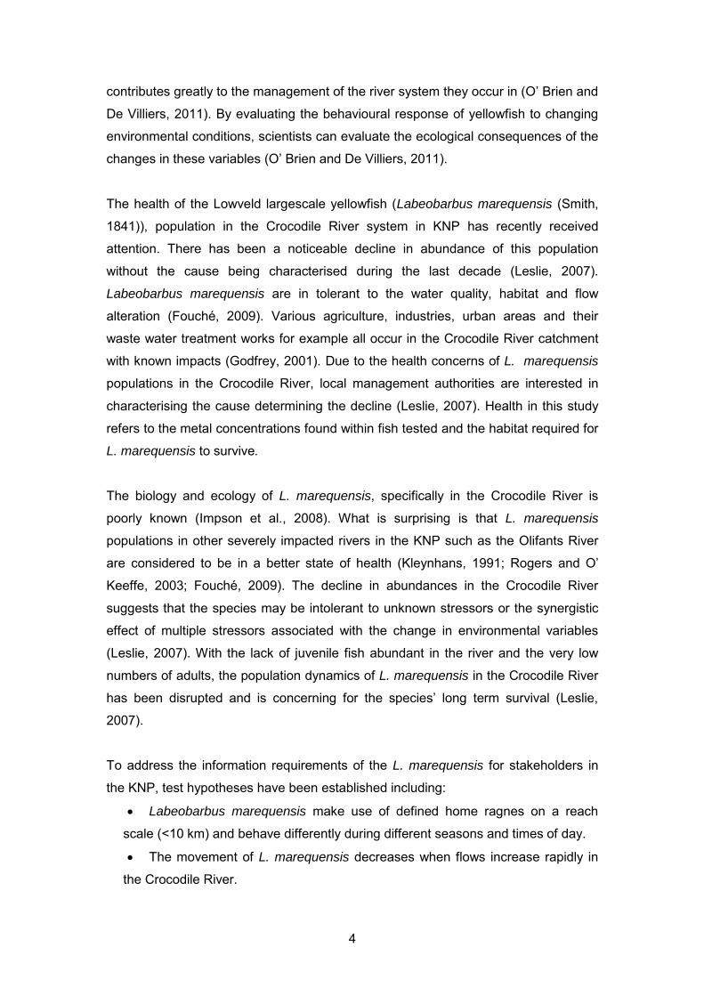
To address the information requirements of the L. marequensis for stakeholders in

the KNP, test hypotheses have been established including:

Labeobarbus marequensis make use of defined home ragnes on a reach

scale (<10 km) and behave differently during different seasons and times of day.

The movement of L. marequensis decreases when flows increase rapidly in

the Crocodile River.

5

The levels of metals in L. marequensis in the Crocodile River are greater than

H. vittatus and C. gariepinus from the Crocodile and Sabie rivers, which negatively

affects the L. marequensis population in the Crocodile River.

The aim of this study is to evaluate the current health, habitat use and movement of

L. marequensis and other fishes in the Crocodile River, KNP. To reach the aims a

behavioural and ecotoxicology assessment of the population of L. marequensis in the

Crocodile River has been undertaken. The objectives of the study Include:

To characterise the home range, habitat use and movement of L.

marequensis and other fishes in the Crocodile River, using biotelemetry methods.

The response of L. marequensis changes in accordance with changing flows

and natural cycles (time of day and seasons) in the Crocodile River.

To determine the extent of metal bioaccumulation in three fish species from

two rivers in the Kruger National Park.

To provide management considerations for the conservation of the L.

marequensis population in the Crocodile River in the Kruger National Park.

The study has been divided into two sections including a behavioural section and

ecotoxicological section. In additional a general introduction, literature survey and

general conclusion with management recommendations has been included as

separate sections. As the structure of this thesis includes:

Chapter 1: Introduction

Presents the rationale of the study, a review of the existing knowledge and

background to the species in question.

Chapter 2: Labeobarbus marequensis species and biotelemetry review

A review of the known biology and ecology of L. marequensis is projected. Relevant

literature regarding its behavioural ecology and ecotoxicological studies specific to L.

marequensis are presented.

Chapter 3: Labeobarbus marequensis behavioural study

This chapter presents the biotelemetry approach adapted in determining habitat use,

and movement for L. marequensis.

Chapter 4: Labeobarbus marequensis ecotoxicology study

6

This chapter presents the bioaccumulation assessment of metals in L. marequensis

and other species within the Crocodile and Sabie rivers, in KNP.

Chapter 5: General conclusions and management recommendations

In this chapter the results from chapter three and four are reviewed and summarized

to suggest ways forward for L. marequensis and the management of the Crocodile

River.

1.1 Study Area

The study area referred to as the Crocodile Site, includes a reach of the Crocodile

River, which forms the southern boundary of the KNP. The site is situated along the

lower sections of the Crocodile River, upstream from its confluence with the Inkomati

River (Figure 1). On the southern bank the Mjejane Game Reserve’s Lodges are

located. The area’s access is controlled because it falls under the mandate of the

KNP to be conserved (Mabunda et al., 2003). Therefore disturbance to wildlife

impacts on the population are minimal. The Crocodile Site is well known for large

specimens of L. marequensis despite their notable decline. Labeobarbus

marequensis have been found to utilize cobble, gravel and deep rocky pools or

rapids (Pienaar, 1978; Russel, 1997; Fouché, 2009). The Crocodile Site is well suited

for the study, in that it is the only stretch of river where these habitats occur

extensively. The rest of the Crocodile River forms long sandy runs and pools (Hill et

al., 2001).

For the ecotoxicological component of the study, a comparative river system was

needed to evaluate the ecotoxicology of the L. marequensis and the other species.

For this the Sabie River was chosen as it also forms part of the Inkomati catchment

and is regarded as having a near-pristine integrity state (Pienaar, 1978; Hills et al.,

2001; Rogers and Luton, 2011). In Figure 1 the geographical areas where the

samples were taken from the Crocodile Site on the Crocodile River and the two

sample sites on the Sabie River are depicted.

7

Figure 1: Shows the location of the Crocodile Site on the Crocodile River and the control

sample sites along the Sabie River, KNP.

8

2 CHAPTER 2: A COMPREHENSIVE LITERATURE REVIEW ON LOWVELD

LARGESCALE YELLOWFISH, LABEOBARBUS MAREQUENSIS

2.1 Introduction

South African “yellowfish” fall under the Genus Labeobarbus and lies within the

family of Cyprinidae. This family composes of all the barbs, yellowfish and labeos.

The genus Labeobarbus is differentiated from other Cyprinidaes in being a large

barbine cyprinid (Skelton, 2001). Within southern Africa the genus Labeobarbus spp.

can be split into two groups, largescale and smallscale yellowfish. The latter of the

two groups are endemic to the South African rivers while L. mareqeunsis are present

in lowveld rivers and L. codringtonii in the upper Zambezi, Okavango and Kunene

rivers (Impson et al., 2008). Oellerman and Skelton (1989) showed Labeobarbus

spp. to be hexaploid, with around 150 chromosomes. Due to this the subgenus was

elevated to full generic status by Skelton (2001). Further their scales are longitudinal

or parallel striae and the primary dorsal fin ray is usually spinous (Skelton, 2001).

The genus Labeobarbus has a poor fossil record and is said to have come from the

mid-Miocene period of East Africa (Skelton and Bills, 2008). Geologist indicate that

systems were all connected at some point in earth’s history and is the cause for close

relatedness between species in now separated river catchments (Skelton and Bills,

2008). The adaption of yellowfish (Labeobarbus spp.) into what we know today was

derived from the nature of the species in a system when more than one species is

present (Skelton and Bills, 2008). This allowed for the diversification of the genus into

the different species that we know today, Labeobarbus intermedius as example has

diversified less than other species, indicating large similarities in the ancestral

yellowfish kind whilst others have adapted to the catchment in which they now occur

(Skelton and Bills, 2008).

The African yellowfishes or Labeobarbus spp. are a well-known charismatic, indicator

fish that are economically important, targeted by dedicated angling industries and

harvested as important sources of protein for many Africans (De Villiers and Ellender,

2008a; Impson et al., 2008; Brand et al., 2009). Being widely distributed in Africa the

lineage constitutes of roughly 80 different species (Skelton and Bills, 2008). Of these

only seven species occur within southern Africa (Skelton, 2001). Angling for

Labeobarbus spp. plays a role in its social and economical importance (Brand et al.,

9

2009). Furthermore as an ecological indicator this genus plays an important role in

the conservation of the ecosystems, as they have been shown to respond to changes

in water quality, quantity and habitat availability (Impson et al., 2008). They thrive in

rivers that have a near natural flow regime and abound in man made lakes that have

diverse habitat, good water quality and few or no alien fishes or plants (Impson et.al

2008).

Apart from being regarded as an abundant species, it is also showing a decline in its

abundance due to the current poor state of South African rivers, (Kleynhans, 1999;

Leslie, 2007; Fouché 2009; Nel et al., 2007). The utilization of water resources and

abuse of angling for the species has lead to concern for the survival and studies on

the different species, there has been very little done for the species L. marequensis

(Impson et al., 2008). The biology and ecology of L. marequensis, specifically in the

Crocodile River is poorly known (Impson et al., 2008). However L. marequensis

populations in other more heavily impacted rivers in KNP such as the Olifants River

are in a better state (Kleynhans, 1991; Seymore et al., 1995; Rogers and O’ Keeffe,

2003; Fouché, 2009). The decline in abundances in the Crocodile River suggests

that the species may be sensitive to unknown stressors or the synergistic effect of

multiple stressors associated with the change in environmental variables. With

juvenile fish low in abundance and the very low numbers of adults in the river, the

population dynamics of L. marequensis in the Crocodile River has been disrupted

and is concerning for the species’ long term survival (Leslie, 2007).

2.2 Labeobarbus marequensis past and present

Genus and Species Labeobarbus marequensis was first referred to by Smith, (1841) as Barbus

marequensis, until Labeobarbus was elevated to full generic status (Skelton, 2001).

The species is widely distributed, its range extends from the middle and lower

Zambezi south to the Phongolo system, with larger specimens generally occurring

below 600m altitude (Skelton, 2001). Their range within the KNP is common

throughout the rivers and tributaries (Pienaar, 1978). They are separated from the

similar largescale species L. condringtoni in distribution and morphology in having a

longer dorsal fin than the head (Skelton, 2001).

10

Conservation The conservation status of L. marequensis is regarded as “Least Concern” as it is still

relatively abundant and widespread in its distribution (IUCN, 2007). Labeobarbus

marequensis within the Crocodile River has had a noticeable decline in the

population and has been found true to other river systems such as the Luvhuvhu

River (Russel and Rogers, 1989; Fouché, 2009). In South Africa L. marequensis

occur in six water management areas (WMA) namely: Crocodile (west)-Marico,

Limpopo, luvhuvhu-letaba, Olifants, Inkomati and the Usuthu-Mhlatuze. Threats that

face L. marequensis are changes in flow regimes, impoundments (man made lakes

and weirs), illegal netting, invasive alien species and degradation of water quality

(Fouché, 2009).

The Kruger National Park is regarded as the stronghold for the conservation of South

Africa’s species including L. marequensis and incorporates a large percentage of its

distribution range in South Africa. Numbers however are said to be declining due to

influences upstream out of the control of the KNP (Russel and Rogers, 1989; Rogers

and O’Keeffe, 2003). The importance of conserving the upper catchment of the river

for the species is much needed in South Africa and has largely been neglected

(Angliss et al., 2005). The declining numbers show the necessity for the

establishment of conservancies (Impson et al., 2008). The fragmentation of rivers is a

concern and the construction of fish-ways at newly planned and existing weirs is a

priority (Impson et al., 2008). Integrated Water Management Areas (WIMA) are also

being developed towards the better management of water resources in South Africa

and will contribute greatly towards the conservation of all aquatic fish species

including, L. marequensis (Rogers and Luton, 2011).

11

2.3 Labeobarbus marequensis biology and ecology

The distribution of L. marequensis is depicted in Figure 2

Figure 2: Distribution range of Labeobarbus marequensis in Africa (after Fouché, 2009).

Morphology

Labeobarbus marequensis has the typical shape of a cyprinid (Figure 3). The species

have 27-33 scales in the lateral line and 12 around caudal peduncle (Skelton, 2001).

The species seldom exceeds 3.5 kgs (7lbs) (Jubb, 1967). In addition the dorsal fin

shows a large degree of variation with Jubb (1967) and Bell-Cross and Minshull

(1988) finding the dorsal fin to decrease in height within its distribution. The dorsal fin

12

height can even vary within a single population (Skelton, 2001). The mouth is

terminally positioned with the mouth-form and lips being variable (Jubb, 1967; Bell-

Cross and Minshull, 1988). Three mouth forms are shown to exist, which according

to Pienaar (1978) have no diagnostic value to the species. Pienaar (1978) further

distinguished the three different mouth forms as forma varicorhinus (square mouth

with chisel-shaped lower cutting jaw), forma gunningi (thick ‘rubber-lips’ form) and

forma typical (intermediate form). The different lip forms are said to be a result of the

species feeding habits and habitat biology (Jackson, 1961; Pienaar, 1978; Skelton,

2001). Colouration of the fish varies from golden yellow in clear water (Bell-Cross

and Minshull, 1988; Skelton, 2001) and pale olive in turbid water (Fouché, 2009).

Figure 3: Picture showing a Labeobarbus marequensis caught within the lower reaches of the

Crocodile River, Kruger National Park.

Growth

Skelton (2001) makes note that large specimens of the species only occur in the

lowveld within its distribution range. Large L. marequensis specimens occur in deep

slow flowing waters, while smaller individuals prefer fast flowing shallow water

(Gaigher, 1969; Fouché et al., 2005). The size class differences of L. marequensis

and the difference in habitat use within those size classes suggested the species

undergoes “ontogenetic shift” (Fouché, 2009). Juveniles and large adult L.

marequenis have the same body length and depth ratios, Fouché, 2009 suggests

that the geomorphological differences influences habitat use at different ages.

Smaller adults of the species are more slender and adapted better for faster flowing

waters (Fouché, 2009). On the Luvhuvhu system low numbers of specimens longer

than a fork length of 180mm within the population of L. marequensis were found

(Fouché, 2009). Skelton (2001) indicates the slow growth of the species.

13

Population structure

Population structure varies between catchment within catchment and changes over

years as discussed under natural reproduction. Within the Luvhuvhu River the male

to female ratio changed over time from 1:3 in the 1960’s to 3.3:1 in 2009 (Gaigher,

1969; Fouché, 2009). Regardless of the shift in sex ratio there was an abundance of

juvenile fish (Fouché, 2009). Large specimens of the species only occur in Lowveld

rivers and further within deep pools in these rivers (Pienaar, 1978; Skelton, 2001).

Large specimens were also only found within the lower reaches of the Luvhuvhu

River with smaller or younger fish occurring throughout the river (Fouché, 2009). To

maintain population structure the population is dependent on a good recruitment from

mature individuals which are long lived and slow growing (Skelton, 2001; Fouché,

2009).

Natural reproduction

Labeobarbus marequensis are serial spawners that have a prolonged spawning

period confirmed by the bi-modal distribution in egg diameter (Fouché, 2009). The

species shows to have two distinct spawning periods a year in southern Africa (May

and September) with the spring spawning period dominating (Fouché, 2009). The

September spawn coincides with increased temperature and changes in discharge

including freshet flows following the onset of major summer rain fall (Fouché, 2009).

Breeding occurs at sites where water flows over boulders and cobbles, riffles and

rapids biotopes or resting areas where mature specimens condition for breeding

(Vlok,1992; Fouché, 2009). Maturity of individual differs within different river systems.

The Luvhuvhu River male L. marequensis mature at fork length 90mm while in the

Inkomati River the species matured at fork length 70mm (Gaigher, 1969; Fouché,

2009). Females of the species differed between the two river systems maturing at

fork lengths 200mm and 280mm in the Luvhuvhu and Inkomati rivers respectively

(Fouché, 2009; Gaigher, 1969). Egg size of L. marequensis are regarded as large

ranging from 0.9mm to 1.2mm, this indicates that embryo have more yolk to feed off

when incubating allowing them to hatch relatively large fish that can avoid predation

(Nikolsky, 1963; Fouché, 2009). The fecundity rate of the species is 44.7 ova per

gram of body mass thus, in a sexually mature female, 200mm fork length, weighing

400 grams, 17,000 mature ova are present in the ovaries (Fouché, 2009). It is still

uncertain if a population will spawn every year or periodically over a number of years

explaining the importance of the large number of eggs produced for the survival of

the species (Fouché, 2009).

14

Migration

Three types of coordinated movement patterns of populations have been described

including: local and seasonal movements, dispersals, and true migrations (Dodson,

1997). Some populations of L. marequensis are known to migrate which is seemingly

associated with spawning during summer and spring (Crass 1964; Pienaar 1978;

Skelton 2001). Fouché (2009) described L. marequensis as spawning migrants

predominantly with an additional small percentage migrating for habitat selection

during non-spawning periods. Possible cues for L. marequensis to migrate include a

complexity of factors varying from flow, water quality and day length (Fouché, 2009).

If the cues are absent despite the condition of fish being ripe for spawning they will

not migrate (Fouché, 2009). Adult L. marequensis have been reported to migrate up

rivers during high flows to spawn in rapids between October and April in Zimbabwe

(Bell-Cross and Minshull, 1988). Although not specific to L. marequensis the

presence of small adult specimens and lack of large adult specimens in fish ladders

during times of high flows in the river suggest that only a portion of the adult

population migrate (Paxton, 2004a).

Food and feeding

Labeobarbus marequensis are opportunistic omnivores that feed primarily on algae

and aquatic insect larvae (midge and mayfly larvae) and small fishes, snails,

freshwater mussels and drifting organisms such as beetles and ants (Crass, 1964;

Skelton, 2001). The relative gut intestinal length of L. marequensis is longer than the

fork length suggesting the fish are herbivorous (Fouché, 2009; Fouché and Gaigher,

2001). Labeobarbus marequensis stomach is straight-tubed and monogastric, it is

funnelled wide at the anterior tapering towards the posterior (Fouché, 2009). There is

no distinct external change-over from the stomach to the intestine and internally there

is no sphincter present at this point, there is a distinct difference between the rugae

of the stomach and the intestines with structural changeover indicating the posterior

boundary of the stomach (Fouché, 2009). The stomach wall had thicker muscular

layers than the rest of the intestines (Fouché and Gaigher, 2001). The length of the

intestinal tract is longer than the fork length with the exception of the smaller classes

of L. marequensis and suggests that small classes may feed off the benthic and

planktonic invertebrates while larger fish are more herbivorous (Fouché, 2009). This

is contrary to Jackson (1961), Crass (1964), Bell-Cross and Minshull (1988) whom

suggest the diet is more carnivorous.

15

Habitat use

Labeobarbus marequensis make use of a variety of habitats. Pienaar (1978)

indicated use of sandy reaches, reed-fringed pools and deep rocky pools below

rapids where the current is swift and strong as habitat use. Russel (1997) showed

preferences to swift-water seams between the rapids and stream margins,

particularly where they have gravel and/or cobble beds. Fouché (2009) found L.

marequensis in both fast-shallow and fast deep habitats. Different age classes are

shown to frequent different habitat types (Gaigher, 1969; Fouché et al., 2005;

Fouché, 2009). Within the Crocodile River the species was found only in the lower

reaches, below 800m and in habitat types characterized by large rocky pools and

runs, rapids and riffles (Kleynhans, 1999). Habitat use is clearly associated with flows

and increased levels of siltation, especially at breeding sites affects habitat use

(Fouché and Gaigher, 2001; Fouché, 2009). In the Crocodile River they were found

within the reaches with a moderate slope indicating moderate flows characteristic of

these reaches (Kleynhans, 1999).

2.4 Labeobarbus marequensis ecosystem service use

The use of riverine ecosystem service use may directly or indirectly affect the

populations of L. marequensis by the use of the ecosystems they occur in. The

relationship and importance of L. marequensis towards humans and the species

effect from human intervention is presented as follows:

Angling stress

Growing interest in the species for angling purpose has brought about the awareness

to practice catch-release angling methods for these species and the slow increase of

private conservation areas currently being established within its natural distribution

will contribute and benefit the conservation of the species (Impson et al., 2008).

Angling on a catch and release basis will be more beneficial to the species as

opposed to fishing for subsistence (Impson et al., 2008). Legislation for bag limits

varies greatly between the provinces within the distribution of L. marequensis. In

KwaZulu-Natal and Limpopo there are no restrictions on the number and size of fish

that may be kept (Impson et al., 2008). In Mpumalanga six fish can be kept with

minimum length of 200 mm and in the North West Province the equivalent figures are

ten and 300 mm respectively. The Yellowfish Working Group (YWG) has

16

recommended a maximum daily bag limit of two fish between 30-50 cm, captured

only by rod and line (Impson et al., 2008).

Ecotoxicology

Although the L. marequensis is considered to be a water quality tolerant species

(Kleynhans, 1991; Fouché 2009) the decline in the population on the Crocodile River

suggests otherwise (Fouché, 2008). Pollard et al. (1996) showed that during periods

of drought in the Sabie River, specimens of L. marequensis were observed to survive

in pools where the electrical conductivity ranged between 200 and 800 Scm-1 and

the dissolved oxygen saturation was low at 50% saturation. It should however be

noted that these conditions probably lasted for short periods (Fouché 2009). Due to

its water quality tolerance, L. marequensis has not received much attention regarding

its importance in indicating changes in water quality related environmental integrity.

Despite this it has been found to be sensitive to flow alterations and increased levels

of siltation, especially at breeding sites (Fouché and Gaigher, 2001). The species has

been used as a bioaccumulation indicator species for metals (Barker, 2006; Seymore

et al., 1995). Although ecotoxicology studies have been done on the species non-

specifically for the Crocodile River have been published. Barker’s (2006) study

served as a baseline study for the Sabie, Shingwedzi, Letaba and Luvhuvhu Rivers

while Seymore et al. (1995) looked at the occurrence of metals in the species and

used it as indication of excessive metal contamination for the Olifants River.

Labeobarbus marequensis metal levels of Cr, Cu, Fe, Pb, Mn, Ni and Zn specific to

the Luvhuvhu and Shingwedzi Rivers were high (Barker, 2006) compared to other

rivers. In the Olifants River the levels were highest in the vertebrae and the gills and

it was suggested to use bony tissues, gills, liver and muscles tissue to test for Mn, St

and Pb (Seymore et al., 1995). In 1994 the species was used in a study on the

Olifants River (KNP) to test for pollutants. Findings were such that over-exposure

from Zn, Cu, Pb and Ni could be sub-lethal (Van Vuren, et al., 1994). Many studies

have used L. marequensis to test for metals within Lowveld Rivers since they all

have similar geological sources (Rogers and O’Keeffe, 2003).

17

3 CHAPTER 3: BEHAVIOURAL STUDY OF AN ADULT POPULATION OF

LOWVELD LARGESCALE YELLOWFISH (LABEOBARBUS MAREQUENSIS)

IN THE CROCODILE RIVER, KRUGER NATIONAL PARK.

3.1 Introduction

Behavioural studies of freshwater fish have contributed to gaining an understanding

of how fish adapt to; optimise the utilisation of the ecosystem resources, successfully

recruit and survive natural and anthropogenic changes in ecosystem conditions

(Godin, 1997; O’ Brien and De Villiers, 2011). A number of behaviour variables of

fishes can be evaluated in a behavioural study including: migration behaviour, habitat

selection, territoriality behaviour, foraging and diet, anti-predator tactics,

reproduction, reproductive strategies and the response of species to changing

environmental variables states (Godin, 1997). This behavioural information of

freshwater fish can contribute greatly towards the understanding of their biology and

ecology. This further will assist in the conservation and management of the species

concerned and their aquatic ecosystems in which they occur (Paxton, 2004b; O’

Brien and De Villiers, 2011).

Telemetry or bio-telemetry has been successfully used as early as the 1950s’ in

acquiring information on the behaviour and physiology of fish and was successfully

used to address and mitigate the impact of stressors on ecosystems (Trefethen,

1956; Cooke et al., 2004). From its origin biotelemetry methods, used to monitor the

behaviour of fish in relation to changing environmental conditions, have been used in

recruitment studies, aquaculture and behavioural studies (Trefethen, 1956; Johnson,

1957; Thorstad et al., 2001; Crook, 2004; Cooke and Schreer, 2003; Cooke et al.,

2004; kland et al., 2005; Tomschi et al., 2009, O’Brien et. al, 2012). This approach

is recognized as the most effective way of acquiring information of wild adult fish over

extended periods and areas to meet specified management questions (Lucas and

Baras, 2000; Rogers and White, 2002; Paxton, 2004a). Due to bio-telemetry’s high

cost it has been limited in its use up until recently and is now becoming more readily

available and affordable (Rogers and White, 2002). Despite the value of telemetry

studies to behaviour of fish, very few have been conducted within freshwater

ecosystems in southern Africa (Thorstad et al., 2001; kland et al., 2003; Paxton,

2004b; Thorstad et al., 2003; kland et al., 2005; O’Brien et al., 2012).

18

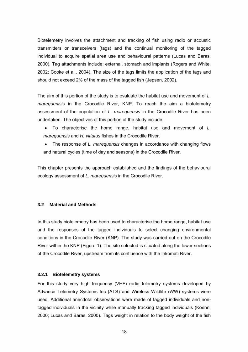
Biotelemetry involves the attachment and tracking of fish using radio or acoustic

transmitters or transceivers (tags) and the continual monitoring of the tagged

individual to acquire spatial area use and behavioural patterns (Lucas and Baras,

2000). Tag attachments include: external, stomach and implants (Rogers and White,

2002; Cooke et al., 2004). The size of the tags limits the application of the tags and

should not exceed 2% of the mass of the tagged fish (Jepsen, 2002).

The aim of this portion of the study is to evaluate the habitat use and movement of L.

marequenisis in the Crocodile River, KNP. To reach the aim a biotelemetry

assessment of the population of L. marequensis in the Crocodile River has been

undertaken. The objectives of this portion of the study include:

To characterise the home range, habitat use and movement of L.

marequensis and H. vittatus fishes in the Crocodile River.

The response of L. marequensis changes in accordance with changing flows

and natural cycles (time of day and seasons) in the Crocodile River.

This chapter presents the approach established and the findings of the behavioural

ecology assessment of L. marequensis in the Crocodile River.

3.2 Material and Methods

In this study biotelemetry has been used to characterise the home range, habitat use

and the responses of the tagged individuals to select changing environmental

conditions in the Crocodile River (KNP). The study was carried out on the Crocodile

River within the KNP (Figure 1). The site selected is situated along the lower sections

of the Crocodile River, upstream from its confluence with the Inkomati River.

3.2.1 Biotelemetry systems

For this study very high frequency (VHF) radio telemetry systems developed by

Advance Telemetry Systems Inc (ATS) and Wireless Wildlife (WW) systems were

used. Additional anecdotal observations were made of tagged individuals and non-

tagged individuals in the vicinity while manually tracking tagged individuals (Koehn,

2000; Lucas and Baras, 2000). Tags weight in relation to the body weight of the fish

19

used in the study ranged between 0.6% and 1.1% of body mass, consistent with the

recommended carrying capacity of fishes (<2%) (Jepsen, 2002).

Advanced Telemetry Systems Inc, (ATS) USA

Advance Telemetry Systems (ATS) was used for the first portion of this study, ATS

tags were used from August 2009 to March 2011. Tags with externally attached radio

transmitters obtained from ATS, three types of transmitters were used (Table 1 and

Figure 4). Each tag transmits a pulse to indicate position of the tag. The tags used

signals within the range of 142.017 to 142.466 MHz at least 10 kHz of each other.

Tagged fish were tracked by foot using a portable ATS-R2100 receiver connected to

a directional 4 element Yagi antennae (Figure 5). The tags battery life lasts from 94

to 366 days with signal transmission set to every 1 second (Table 1). In addition an

ATS receiver, model R4500S (Receiver/ Datalogger with DSP), was use in a remote

station to under take remote monitoring. The station had two antennae positioned 90

angle apart one facing upstream and the other downstream to indicate up and down

movement of the tags in the river (Figure 5). The station needed to be as close to the

river to maximise its use. The station was erected at location S 25.37880 E

031.714350 (GPS co-ords in dec.deg).

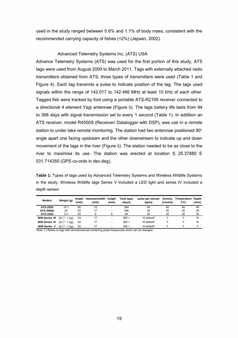
Table 1: Types of tags used by Advanced Telemetry Systems and Wireless Wildlife Systems

in the study. Wireless Wildlife tags Series V included a LED light and series IV included a

depth sensor.

ATS-2030 10.1 50 12 - 264 40 40 40 40ATS-2060b 22 53 17 - 366 35 35 35 35ATS-1930 2.4 25 9 6 94 30 30 30 30

WW-Series Ill 20 (+/_ 1.5g) 53 17 - 365 + 10 default* Y Y NWW-Series IV 20 (+/_ 1.5g) 53 17 - 365 + 10 default* Y Y NWW-Series V 20 (+/_ 1.5g) 53 17 - 365 + 10 default* Y Y Y

Note: (*) Refers to tags with remote/manual monitoring pulse frequencies which can be changed.

Activity

(counts)

Temperature

(C)

Depth

(mm)

pulse per minute

(ppm)Models Weight (g)

Time span

(days)

height

(mm)

diameter/width

(mm)

length

(mm)

20

Figure 4: Advanced Telemetry Systems’ tags, models 2030, 2060 (A) and 1930 (H) used in

the study and attached to fish. Hydrocynus vittatus with an ATS 2060b transmitter (B),

Labeobarbus marequensis with an ATS 2030 transmitter (E) and 1930 transmitter (I).

Wireless Wildlife Systems’ tags, Series III (D), Series IV (G) and Series V (K) used in the

study attached to Hydrocynus vittatus (C) and Labeobarbus marequensis (F and J).

Wireless Wildlife (WW) RSA

From September 2011 onwards WW systems were used. Tags with externally

attached radio transmitters obtained from WW, three types of tags were used in the

study (Table 1 and Figure 4). Tagged fish were tracked by foot using a portable note

book connected to a directional 4 element Yagi antennae (Figure 5). The lifespan of

all WW-tags have a battery lifespan of 365 days (based on battery life expectancy

with an 80 % safety factor) by combining default and active tracking modes. Defaults

modes include on of the digital transmission sent every ten minutes. This can be

changed to transmissions every 1 sec, 2 min and 5 min depending on the type of

monitoring required (remote or manual). During field monitoring, transmissions are

changed to 1 sec mode in order to intensively follow and track the fish. After a

monitoring session, the transmissions are switched back to 10 minutes by default in

order to conserve the tags battery life.

IH

E

D

C

F

G

BA

K

J

IH

E

D

C

F

G

BA

K

IH IH

EE

D

C

D

C

F

G

F

G

BBAA

K

J

21

Figure 5: Advance Telemetry System’s manual monitoring (A) equipment used during the

study and Wireless Wildlife’s manual monitoring (D and E) used during the study with a base

station and relay station (C) used for remote monitoring.

A

B C

D

E

A

B C

D

E

22

Receivers were used to track the tags; this included both a notebook (small laptop)

with WW tracking software installed and an Omni-antennae or directional Yagi

antennae for manual tracking with a network of station set up strategically over the

Crocodile Site for remote tracking (Figure 5). Each tag has additional sensory

components, including: an activity sensor, measured in counts, temperature sensors

measured in degrees Celsius and depth measured in cm.

Five remote monitoring stations were constructed for the study this included 1 base

station and 4 repeater stations. The repeaters were remote receivers which transmits

data acquired from tags within its coverage to the base station. The base station

transmits all data it receives from the repeaters and tags in its coverage and sends

that data through to a survey at WW (Figure 6).

Figure 6: Placement of the remote stations used for the Wireless Wildlife system covering the

Crocodile Site. The signal range for each station is indicated by colour, yellow being the

strongest to red being the weakest.

3.2.2 Capture and tagging

Adult L. marequensis weighing more than two kilograms were captured using a range

of sampling techniques (Figure 7). All fish caught were obtained using the following

techniques: angling techniques, electro-shocker (220 V) and gills nets in deep (>1.5

m) areas. The various fishing techniques were used in order to get a good descript of

the population (Rogers and White, 2002).

23

Figure 7: Capture techniques, Fly fishing (A and G), bait fishing with worms, corn and crickets (E and F), Netting (D), electro-fisher (220 V) (B) and Casting nets

(C) were used in order to obtain suitable fish for the study.

F

24

Captured fish were immediately placed in an aerated anaesthesia container

containing clove oil (0.5 ml.l-1) and sedated until signs of narcosis became evident

(Figure 8) (O’Brien et al., 2012). This was indicated by the fish losing its ability to

maintain its orientation. A transmitter was attached by inserting two anchoring wires

through the musculature of the L. marequensis at the base of the dorsal fin. Two

spinal needles were pushed through the sedated individual; anchoring wires attached

to the transmitter are then threaded through the spinal needles. Plastic washers and

metal sleeves were then attached to the loose end of the anchoring wires and then

secured in placed by crimping the metal sleeves. The excess anchoring wire was

then clipped off. During the recovery phase the fishes measurements were taken

namely: weight, standard length, fork length, total length and the girth (Figure 8). The

fish was then allowed to recover fully and released once it could swim away strongly

on its own accord. The recovery and early behaviour of the fish is monitored after

capture and tagging. This allowed for an assessment of the effect of the capture and

tagging procedure on the fish. Two weeks were given to each individual before

perceived natural behavioural activities were documented (Rogers and White, 2002;

O’ Brien and De Villiers, 2011, O Brien et al., 2012).

A minimum of 2% body:tag ratio meant that the individuals used for the study were all

above 2 kg and exceeded the minimum fork length of adults reaching sexual maturity

(Fouché 2009; Gaigher, 1969; Jepson, 2002). All fish were captured, tagged and

release within the Crocodile Site with the exception of one individual fish (LMAR8)

which was captured, tagged and released within 5km upstream from the Crocodile

Site.

In addition to L. marequenis suitable Hydrocynus vittatus individuals were also

considered in the study for comparative purposes (Table 2). The same capture,

tagging and tracking techniques established for L. marequensis were implemented

for the H. vittatus individuals.

25

Figure 8: The tagging procedures included: capture fish and the equipment needed to tag the fish (A). The fish is anaesthetised before operating and then

submerged back into the water once the spinal needles have been inserted to start recovery (B, C). The spinal needles are inserted through the muscle below

the dorsal fin and anti-biotics applied into the needles to coat the anchoring wires from the transmitter (D, E). Plastic and metal sleeves are placed onto the

coated anchoring wires and crimped (F) more anti-biotics are applied around the tag and above the head (G). Fish measurements are recorded (H) the fish

recovery starts (I) and the fish once fully recovered allowed to swim away freely (J, K).

E

D

F

B

A C

I JH

G

K

E

D

F

B

A C

I JH

G

K

26

Table 2: Species, tag type, capture location, monitoring period from capture date to the last day monitored (end date) and fixes during manual

and remote monitoring during the study.

Name Tag type Tag no. Mass (g) Capture Date End Date Days

tracked

Manual monitoring

fixes

Remote monitoring

fixesLMAR1 ATS-2030 142.214 2500 -25.37942 31.71041 15/08/2009 19/09/2009 35 15 -LMAR2 ATS-1930 142.232 1800 -25.37872 31.71271 15/08/2009 15/05/2010 273 30 -LMAR3 ATS-1930 142.113 2200 -25.37804 31.70758 15/08/2009 1/12/2009 108 16 -LMAR4 ATS-1930 142.092 2100 -25.37804 31.70758 16/08/2009 15/05/2010 272 42 -LMAR5 ATS-2030 142.153 2500 -25.37872 31.71271 16/08/2009 17/02/2011 550 109 -LMAR6 ATS-1930 142.051 2100 -25.37872 31.71271 16/08/2009 15/05/2010 272 42 -LMAR7 ATS-1930 142.032 3000 -25.22722 31.71271 19/09/2009 15/05/2010 238 65 -LMAR8 ATS-1930 142.072 2500 -25.39905 31.6784 19/06/2010 16/02/2011 242 46 -LMAR9 ATS-2030 142.014 2600 -25.37884 31.71291 17/09/2010 14/11/2010 58 19 -LMAR10 WW-Series II 6 2550 -25.3784 31.7197 19/09/2011 01/06/2012 232 8 6602LMAR11 WW- Series I 25 2875 -25.3784 31.7197 19/09/2011 01/06/2012 232 7 2229LMAR12 WW-Series II 7 2550 est -25.3784 31.7197 19/09/2011 01/06/2012 232 2 6116LMAR13 WW- Series I 17 2300 est -25.3784 31.7197 19/09/2011 01/06/2012 232 4 316LMAR14 WW- Series I 12 2250 est -25.37885 31.71478 19/09/2011 01/06/2012 232 - 3324LMAR15 WW- Series I 14 2300 -25.3784 31.7197 15/10/2011 01/06/2012 206 - 479LMAR16 WW-Series IV 42 3900 -25.3784 31.7197 29/11/2011 01/06/2012 161 - 1262HVIT1 ATS-2060b 142.322 1300 -25.37884 31.71469 19/08/2009 19/09/2009 31 1 -HVIT2 ATS-1930 142.132 500 -25.37884 31.71469 19/08/2009 - - - -HVIT3 WW- Series I 21 2200 -25.37864 31.71333 16/09/2011 01/06/2012 235 - 1552HVIT4 WW- Series I 23 1380 -25.22438 31.42529 19/09/2011 01/06/2012 232 - 58HVIT5 WW- Series I 19 2580 -25.37871 31.71586 19/09/2011 01/06/2012 232 - 1626HVIT6 WW- Series I 9 1750 -22.22422 31.43179 19/09/2011 01/06/2012 232 - 3702HVIT7 WW- Series I 13 2100 -22.22422 31.43179 22/09/2011 01/06/2012 229 74 6774HVIT8 WW- Series I 15 4000 -22.22422 31.43179 20/10/2011 01/06/2012 201 - 1834HVIT9 WW- Series I 16 2000 -25.37885 31.71478 04/11/2011 01/06/2012 186 - 2272HVIT10 WW-Series IV 41 3000 -25.22394 31.44291 23/11/2011 01/06/2012 167 - 899HVIT11 WW- Series I 31 2100 -22.22422 31.43179 26/11/2011 01/06/2012 164 - 236HVIT12 WW- Series I 35 2000 -25.2249 31.42282 28/11/2011 01/06/2012 162 - 224

Note: LMAR = Labeobarbus marequnesis ; HVIT = Hydrocynus vittatus

Capture location (GPS location)

27

3.2.3 Monitoring techiniques

The manual monitoring approaches involved the tracking or homing of the tagged

fish during the study using the ATS or WW receivers and directional Yagi antennae.

Manual monitoring methods used were based on techniques established by O’ Brien

and De Villiers (2011) (Figure 9). Tagged individuals were monitored from the banks

of the Crocodile River, the narrow width of the river allowed for easy access to

accurately (<1m from the observer) find fish. Weekly manual monitoring surveys

were scheduled on a monthly basis throughout the year. This allow for a seasonal

bio-telemetry evaluation. Habitat preferences and movement variables of the tagged

fish were monitored and captured using data sheets and a field diary of anecdotal

events. These variables included intra- and inter-species variation in the area where

the fish were monitored (Godin, 1997).

The remote monitoring approaches involved the setting up of a coverage station

allowing the continual tracking of individuals within the Crocodile Site. Data were then

downloaded to a data management system (DMS) that could be accessed using an

internet interface WW system or downloaded directly onto a personal computer. The

ATS remote monitoring system made of one remote monitoring station and could

obtain signals from tags up to 1000 m from the station. Two directional antennae

were used to locate tagged fish up or down stream from the remote monitoring

station. The WW remote monitoring network consisted of a base station and four

relay stations that received data from the tag between 500 m to 1000 m from the

remote monitoring stations. This included additional monitoring components which

allowed for the continuous (every 10 minutes) monitoring of the tag individual. These

data could be retrieved in real time from the DMS.

28

Figure 9: Schematic diagram presenting the monitoring methods followed out during monitoring surveys adopted from O’Brien and De Villiers (2011)

29

3.2.4 Habitat preferences

This included the consideration of the spatial behaviour (location and associated

movement) in relation to available cover features and habitat biotopes measured using

manual monitoring techniques. To determine the spatial behaviour of the fish the location

of the tags within the Crocodile Site were used.

Spatial behaviour

The home range has been defined as the spatial range measured between the maximum

upstream and downstream movement of a tagged individual over a certain time frame

(Hodder et al., 2007). This is the area of a river that an organism requires to acquire food,

shelter and breed successfully (Hodder et al., 2007). The home ranges of individuals

monitored were evaluated using the known locations of tagged individual and the area in

which they occurred whilst monitoring. Geographical Information Systems (GIS) were

implemented to demarcate the home ranges utilised during the study by L. marequensis.

Cover features

Kramer et al. (1997) argues that the behaviour of the fish is orientated around the

particular habitat most suitable for (maximising) the survival and reproductive success of

an individual. Environmental variables were documented in an attempt to evaluate any

existing relationships between the environmental variables and L. marequensis movement

in the study. Table 3 shows the habitat variables measured within the study, these were

adapted from O’ Brien and De Villers (2011). Habitat cover features specifically for fish

included the consideration of the use of and or availability of undercut banks or root wads

(UBRW), dead and or submerged trees (S-trees), complex substrate types such as

boulder beds (S-boulders), rocky outcrops or emerging boulders (E-boulders) and

submerged ridges (S-ridge), marginal aquatic (M-veg) and emergent vegetation (E-veg),

island, water column and the top of or tail out of pools. Primary and secondary habitat

types associated with tagged fish locations were considered to ensure that the area where

the L. marequensis was found was descriptive of the area.

30

Table 3: Spatial habitat data associated with the observed locations and movement of the tagged

L. marequensis monitored during the study.

Behaviourable Variable Substrate Surface types Habitat availability Colour Weather

Maximum deisplacement

per MinuteSilt No flow Undercut bank/roots Clear Clear

Sand Barely perceptible flow Dead/submerged trees Opaque overcastGravel Smooth and turbulent Submerged-Boulders Light brown cloudyCobble Ripple surface Emerging-Boulders Dark chocolate lightrain

Boulder Undular/broken standing waves Submerged-Ridge heavy rain

Bed Rock Free falling Marginal VegetationChaotic flow Aquatic VegetationVerticle flow Water Colum

Wind Ripple Surface

Habitat biotopes

Habitat biotopes included the availability and use of surface flow types and substrate type

combinations or geomorphological habitat units as defined in Hirschowitz et al. (2007).

Table 3 presents the surface flows and substrate types recorded in order to determine

biotopes where tagged individuals were frequently found, such as runs, riffles rapids

backwater areas, pools and glides (Hirschowitz et al., 2007).

3.2.5 Behavioural variables

A behavioural variable used in this portion of the study was movement measured either in

activity counts (remote monitoring) or as maximum displacement per minute (MDPM) in

metres per minute (m.min-1). Depth was included as measurable behavioural variable. The

MDPM includes the recorded displacement (m) of the fish during a five minute manual

monitoring period spaced over ten minute intervals. The MDPM was recorded by

estimating the distance (in metres) a fish moved during a five minute observation period

and then calculated into metres per minute. Activity for remote data was measured in

counts per minute while depth was measured in mm.

Natural cycles (time of day and seasons) and discharge

The behavioural variables were compared within six time of day (TOD) intervals, season

intervals and established discharge classes according to flows observed during the study.

Time of day intervals considered included: 00h00-04h00, 04h00-08h00, 08h00-12h00,

12h00-16h00, 16h00-20h00 and 20h00-24h00. Seasons were determined by three month

periods starting from December to February (summer), March to May (autumn), June to

31

August (winter) and September to November (spring). Flow classes were determined

using existing flows over the duration of the study obtained from Department of Water

Affairs (DWA) (Station number: X2H046Q01 Crocodile River at Riverside/Kruger National

Park) and then divided in to three flow classes namely: low flows (0 m3.s-1 to 10 m3.s-1),

moderate flow (10 m3.s-1 to 60 m3.s-1) and high flows (>60 m3.s-1).

3.2.6 Data analysis

Behavioural and environmental variables were broken down into seasons and then

analysed using statistical and descriptive statistical techniques. Location and movement

data were analysed using spatial analysis software (ARC GIS ®), this approach allows for

the assessment of spatial behaviour of individuals, the high use, preferred areas and some

relationships between the locations of the tagged fish and the state of general

environmental variables as shown in Hodder et al. (2007). Descriptive statistical analyses

included the use of Windows Excel, (©2011, Microsoft Corporation). Ecosystem variable

data associated with the behaviour of L. marequensis was recorded using primary

variables (scored first) and secondary variables (scored second) and then combined with a

weighting variable of a 2:1 ratio (primary variables: secondary variables). This indicated

the importance of the tagged individual’s immediate variables associated with the tagged

fish as well as any nearby important other variables. To determine movement patterns for

cover features and biotopes, previously described time intervals, seasonal intervals and

flow classes (see material and methods). Remote and manual behavioural data were

analysed separately using MDPM and activity counts as the behavioural variable

(movement) respectively (O’ Brien et al., 2012). This was done using a mixed-model

analysis of variance (ANOVA) approach with a random coefficients model (Littell et al.,

1996) and Akaike’s information Criteria (AIC) model selection (Burnham and Anderson,

1998) were used. Analyses were conducted using SAS version 9.3 (SAS Institue, Cary,

NC).

3.3 Results

Of the 16 L. marequensis and 12 H. vittatus monitored in the behavioural study, nine of the

L. marequensis and two H. vittatus were attached with ATS tags and the remainder with

WW tags. Labeobarbus marequensis mean weight was 2464.1 g (SD=476.6 g) with the

32

mean standard length 453 mm (SD=33.8 mm). Hydrocynus vittatus mean weight was

1874.8 g (SD=879.7 g) with the mean standard length 45 mm (SD=81.2 mm) (Table 2).

Advance Telelmetry Systems and WW manual monitoring observations totalled 479 fixes

from 15 individuals (Table 2). Wireless Wildlife remote monitoring observations totalled

39505 strings of data from 17 individuals; two were tagged with WW-series v (depth

censor) tags (Table 2). Remote monitoring from the ATS system recorded over 44171

strings of data over a period from the 21 September 2010 to 12 November 2010. Wireless

Wildlife tags obtained 20327 L. marequensis and 19130 H. vittatus strings of data for

movement and 1262 L. marequensis and 899 H. vittatus strings for depth. Wireless wildlife

tags were only able to obtain remote seasonal data for spring, summer and autumn for

activity counts and spring and summer for depth.

3.3.1 Habitat Preference

Spatial behaviour

The location of individuals LMAR 1-9 was plotted within in the Crocodile Site and mapped

to depict the home range of each individual could be depicted (Figure 10, 11 and 12).

These individuals were selected as there were sufficient data to graphically depict their

movements along the Crocodile Site. This showed that L. marequensis preferred the reach

of river around the Crocodile Site. The remote data from the ATS remote station showed

that LMAR5 and LMAR9 were found constantly in the Crocodile site for a period of two

months before the station was destroyed during floods. Key areas were identified within

the Crocodile Site which was used frequently by tagged individuals (Figure 13).

33

Figure 10: The home ranges of Labeobarbus marequensis for individuals LMAR 1 (A), LMAR 2 (B)

and LMAR 3 (C).

AA

BB

CC

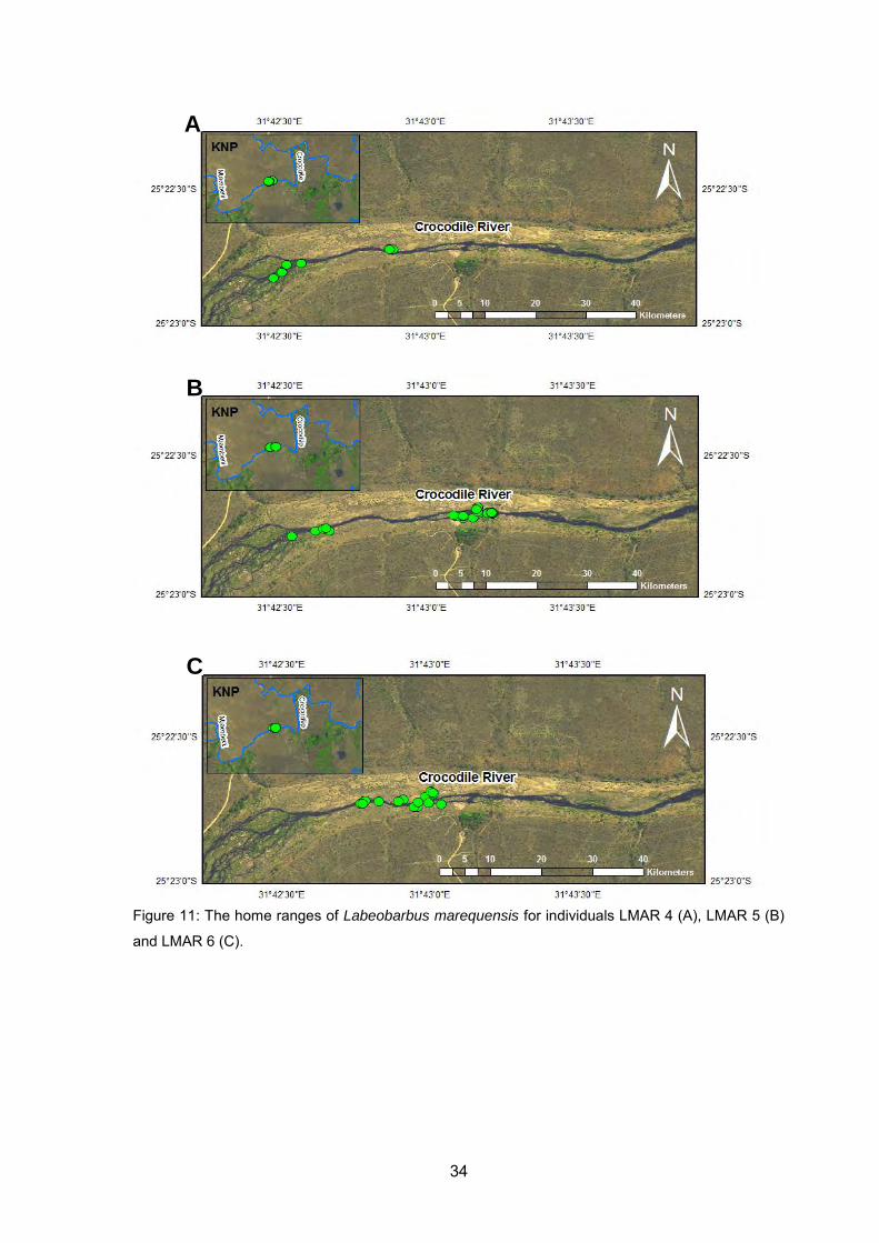
34


and LMAR 6 (C).

BB

CC

AA

35


and LMAR 9 (C).

B

C

A

36

Figure 13: Depicts the key sites L. marequensis, with their referenced names, along the Crocodile

River study area.

Fish caught and tagged in a location had a tendency to return to and frequently be found

within its tagged location (Table 2). This was evident with LMAR3 and LMAR4 individuals.

All individuals show clear home ranges with high frequency to key areas with distinct cover

features and habitat biotopes (Table 4). Fish LMAR3 and LMAR4 were frequently

associated with key area 1 (Figure 13 and 14). Two other distinct channel types were key

area 3 and key area 4 (Figure 13 and 14). The key area 3 had a deep run (through bed

rock) and opened up into a reeded southern bank and bedrock northern bank with back

flow, while key area 4 had a pool flowing into a run with a reeded southern bank and

bedrock northern bank. This location was well utilized by tagged individuals LMAR 1,

LMAR 6, LMAR 7 and LMAR 4. Individuals LMAR2 and LMAR5 were frequently found

together in the reach of river named area 4. It must be noted that at the key area 4 in the

channel produced five of the L. marequensis of tagging criteria for the WW component of

the study. Where as the other locations were not nearly as active with L. marequensis in

2011 than in 2009 (Table 2).

Table 4: Cover Features and Habitat Biotopes for the key area’s within the Crocodile Site

Area Dominant cover feature Habitat biotopes

1 Emerging Boulders, Marginal Vegetation Run2 Submerged Boulders, Emerging Boulders Glide3 Submerged Boulders, Marginal Vegetation Glide4 Submerged Boulders, Marginal Vegetation Glide and Run

Key area 1 Key area 2 Key area 3 Key area 4

37

Figure 14: Pictures depicting the key areas in the Crocodile Site and main habitats where tagged

individuals were found most frequently: Key area 4 (A); A channel (B); Key area 3 (C); the location

where LMAR2, LMAR5, LMAR6 and LMAR9 were tagged (D and E); Key area 2 (G, H) where LMAR1

was tagged; Key area 1 where LMAR3 and LMAR4 were tagged and found regularly (F)

FD

C

E

B

A

G H

FD

C

E

B

A

G H

38

Cover features

Differences in the cover features associations between L. marequensis and H. vittatus

were found. Hydrocynus vittatus was more commonly (33 %) associated with aquatic

vegetation than L. marequensis (1.4 %). Submerged boulders were used by both species

frequently, 32.4 % and 66.7 % for L. marequensis and H. vittatus respectively. There was

a significant increase in movement for L. marequensis when associated with S-boulder

cover than any other cover feature tested (p=0.0001). The most frequently visited cover

feature was S-boulders (32.38 %). The other habitats that took preference were habitats of

similar description being UBRRW (22.92 %), E-boulders (13.37 %) and M-veg (12.76 %)

all having some permanent structure with the exception of M-veg. A-veg (1.39 %) along

with substrate ridge (1.39 %) was the least presented cover feature (Figure 15).

Figure 15: Cover features (A and B) and Biotopes preference of L. marequensis (A and C) and H.

vittatus (B and D).

The movement of the L. marequensis and H. vittatus differed between seasons and flow

discharge categories, Seasonal differences were associated with day length and

HabitatUBRW

S-trees

S-boulders

E-boulders

S-ridge

M-veg

Water coloum

A-veg

Habitat

1 2

BackwaterPoolGlideRunRiffle


Undercut bank/Root wadSubmerged TreeSubmerge BoulderEmerging BoulderSubmerged RidgeMarginal VegetationWater ColumAquatic Vegetation


A

C D

B

L. marequensis

HVIT





A

C D

B

H. vittatus

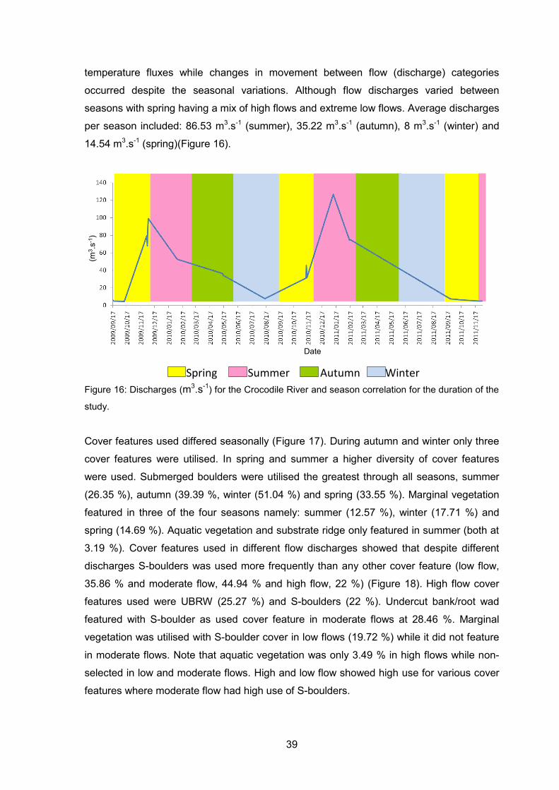
39

temperature fluxes while changes in movement between flow (discharge) categories

occurred despite the seasonal variations. Although flow discharges varied between

seasons with spring having a mix of high flows and extreme low flows. Average discharges

per season included: 86.53 m3.s-1 (summer), 35.22 m3.s-1 (autumn), 8 m3.s-1 (winter) and

14.54 m3.s-1 (spring)(Figure 16).

Figure 16: Discharges (m3.s-1) for the Crocodile River and season correlation for the duration of the

study.

Cover features used differed seasonally (Figure 17). During autumn and winter only three

cover features were utilised. In spring and summer a higher diversity of cover features

were used. Submerged boulders were utilised the greatest through all seasons, summer

(26.35 %), autumn (39.39 %, winter (51.04 %) and spring (33.55 %). Marginal vegetation

featured in three of the four seasons namely: summer (12.57 %), winter (17.71 %) and

spring (14.69 %). Aquatic vegetation and substrate ridge only featured in summer (both at

3.19 %). Cover features used in different flow discharges showed that despite different

discharges S-boulders was used more frequently than any other cover feature (low flow,

35.86 % and moderate flow, 44.94 % and high flow, 22 %) (Figure 18). High flow cover

features used were UBRW (25.27 %) and S-boulders (22 %). Undercut bank/root wad

featured with S-boulder as used cover feature in moderate flows at 28.46 %. Marginal

vegetation was utilised with S-boulder cover in low flows (19.72 %) while it did not feature

in moderate flows. Note that aquatic vegetation was only 3.49 % in high flows while non-

selected in low and moderate flows. High and low flow showed high use for various cover

features where moderate flow had high use of S-boulders.

Spring Summer Autumn Winter

Date

(m3 .s

-1)

40

Figure 17: Cover features (A-D) and Biotopes (E-H) of Labeobarbus marequensis for different seasons, Summer (A and E), Autumn (B and F), Winter (C and

G) and Spring (D and H).

Autumn WinterSpring

SummerUndercutBank/Root

SubmergedTrees

Substrate-Boulders

Emerging-Boulders

Substrate-Ridge

MarginalVegetation

Water coloum

AquaticVegetation

DCA B

HGE F

Summer

Backwater Pool Glide Run Riffle

Spring


Aut umn


Wint er


Backwater Pool Glide Run RiffleBackwater Pool Glide Run Riffle

Undercut bank/Root wad Submerged Tree Submerged BoulderMarginal Vegetation Water Colum

Emerging BoulderSubmerged Ridge Aquatic VegetationUndercut bank/Root wadUndercut bank/Root wad Submerged TreeSubmerged Tree Submerged BoulderSubmerged Boulder

Marginal VegetationMarginal Vegetation Water ColumWater ColumEmerging BoulderEmerging Boulder

Submerged RidgeSubmerged Ridge Aquatic VegetationAquatic Vegetation

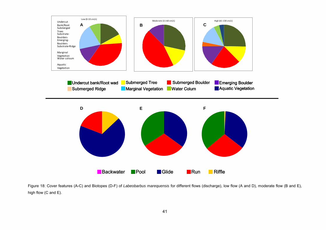
41

Figure 18: Cover features (A-C) and Biotopes (D-F) of Labeobarbus marequensis for different flows (discharge), low flow (A and D), moderate flow (B and E),

high flow (C and E).

FED

Backwater Pool Glide Run RiffleBackwater Pool Glide Run Riffle

Low (0-10 cm/s)UndercutBank/RootSubmergedTreesSubstrate-BouldersEmerging-BouldersSubstrate-Ridge

MarginalVegetationWater coloum

AquaticVegetation

Moderate (11-60 cm/s) High (61-130 cm/s)

CBA

Undercut bank/Root wad Submerged Tree Submerged BoulderMarginal Vegetation Water Colum

Emerging BoulderSubmerged Ridge Aquatic VegetationUndercut bank/Root wadUndercut bank/Root wad Submerged TreeSubmerged Tree Submerged BoulderSubmerged Boulder

Marginal VegetationMarginal Vegetation Water ColumWater ColumEmerging BoulderEmerging Boulder

Submerged RidgeSubmerged Ridge Aquatic VegetationAquatic Vegetation

42

Habitat biotopes

Habitat biotopes used by L. marequensis were glides 55 % of the time. Run and pool

biotopes had high preferences with 21.2 % and 11.9 % respectively. Hydrocynus

vittatus were associated with different habitat biotopes than L. marequensis

frequenting the riffle biotopes. This showed L. marequensis used deeper biotopes

than that of H. vittatus.

Biotopes used in different season varied in a manner similar to that of cover features

(Figure 17). Autumn and winter had only three frequented biotopes whilst summer

and spring had a high diversity of biotopes frequented. Riffle biotopes being

frequented in autumn more than in the other seasons. Glide biotope types were

dominated throughout all season for L. marequensis. In winter pools, glides and runs

were higly utilised. Habitat biotopes during moderate and high flows showed similar

uses for glide, pool and run. Low flows had the most diverse biotope use.

3.3.2 Behaviour variables

The influences of the natural cycles on the movement of L. marequensis showed to

change within the time of day, season and discharges. Further depth preferences

were found across these natural cycles.

Time of day

Labeobarbus marequensis exhibited diurnal activity with heightened movements

during mid-day. While H. vittatus displayed crepuscular movements that were

heightened during the early mornings (Figure 19). Increases in movement were also

associated with depths of L. marequensis over the day period increasing during

midday while H. vittatus depth increased during early morning periods (Figure 19).

43

Figure 19: The movement (activity counts) (A and B) and depth (mm) (C and D) relationship

between time of day for Labeobarbus marequensis (A and C) and Hydrocynus vittatus (B and

D).

Seasons

Labeobarbus marequensis movement increased during spring while decreasing from

spring through to autumn (Figure 20). Depth from spring to winter also change in that

L. marequensis took up shallower depths in summer than in spring. Hydrocynu

vittatus had insufficient data over seasons to determine difference between seasons.

370

380

390

400

410

420

430

440

450

00

h-0

4h

n=

27

0

04

h-0

8h

n=

24

3

08

h-1

2h

n=

16

4

12

h-1

6h

n=

19

4

16

h-2

0h

n=

19

8

20

h-2

4h

n=

19

3

0

5000

10000

15000

20000

25000

00h-

04h

n=36

07

04h-

08h

n=32

75

08h-

12h

n=32

86

12h-

16h

n=34

09

16h-

20h

n=34

07

20h-

24h

n=33

43

0

2000

4000

6000

8000

10000

12000

14000

16000

18000

00h-

04h

n=34

90

04h-

08h

n=37

81

08h-

12h

n=22

24

12h-

16h

n=30

57

16h-

20h

n=35

59

20h-

24h

n=30

39Hours Hours

(mm

)

Hours Hours

(cou

nts)

(cou

nts)

L. marequensis H. vittatus

A B

C D

0

100

200

300

400

500

600

00h-

04h

n=14

1

04h-

08h

n=22

1

08h-

12h

n==1

14

12h-

16h

n=15

6

16h-

20h

n=15

9

20h-

24h

n=10

8

(mm

)

(mm

)

(mm

)

A B

44

Figure 20: The movement (activity counts) (A) and depth (mm) (B) relationship between

seasons for Labeobarbus marequensis.

Flow (discharge)

Flows showed to have an effect on the movement of L. marequensis in that during

low and moderate flows movement was higher than in high flows where almost no

movement was found (Figure 21). Depth preferences were more variable during low

flows than moderate flows. Hydrocynu vittatus had insufficient data over seasons to

determine difference between seasons.

Activity Depth

Season Season

(cou

nts)

(mm

)

A B

0

2000

4000

6000

8000

10000

12000

14000

16000

18000

20000

Sp

rin

gn

=1

52

45

Su

mm

er

n=

50

02

Au

tum

n n

=8

0

370

380

390

400

410

420

430

440

450

Sp

rin

g n

=54

Su

mm

er

n=

120

8

Activity Depth

Discharge Discharge

(cou

nts)

(mm

)

A B

370

380

390

400

410

420

430

440

Low

0-1

0 m

3/s

n=10

30

Mod

erat

e 10

-60

m3/

s n=

232

0

2000

4000

6000

8000

10000

12000

14000

16000

18000

20000

Low

0-1

0 m

3/s

n=97

27

Mod

erat

e 10

-60

m3/

sn=

1046

6

Hig

h 60

-nm

3/s

n=13

4

45

Figure 21: The movement (activity counts) (A) and depth (mm) (B) relationship between flows

(discharges) for Labeobarbus marequensis.

3.4 Discussion

3.4.1 Habitat preferences

The GIS data showed that L. marequensis establish home ranges within the study

area with some individuals establishing focal areas. No observations of fish migrating

out of the Crocodile Site were observed indicating the use of the Crocodile Site as

there home range. Within these home ranges fish frequented specific locations over

other locations. This suggests that the population sample is specific to the Crocodile

Site showing the importance of these biotopes and cover feature found within the

reach, unlike the rest of the Crocodile River (Hill et al., 2001). Furthermore this

suggests that adult L. marequensis in the Crocodile River have relatively small home

ranges and do not use reaches (>5 km) of the river extensively. The sessile

behaviour of the adult L. marequensis (>2 kg) observed in the study suggests after

maturity home ranges are established in small reaches that meet their biological

functioning. The extent of these home ranges appears to be dependent on the

availability of habitats and will possibly be affected by population pressure. Fouché

(2009) showed that L. marequensis exhibit reach scale migrations that may exceed

50 km. These migrations may involve smaller sub-adult L. marequensis.

Cover features and habitat biotopes used by L. marequensis were found to be similar

to that described by Pienaar (1978) apart from sandy reaches which appeared to be

avoided by the tagged individuals. Contrary to what Fouché (2009) described this

study showed that large L. marequensis frequented slow, deep habitat types as

apposed to fast, deep and fast, shallow habitats depending on the age of the fish.

Further, this study showed that L. marequensis frequent different habitats during

different seasons and flows. Habitat use during different seasons and flows has not

previously been described for adult L. marequensis. Seasonal changes determine

the daylight length and its effects on an organism. In this study adult L. marequensis

showed to frequent various habitat biotopes and cover features during summer and

spring, differing to winter and autumn. This indicates some form of change in their

biology during those seasons which may cause various habitat biotopes and cover

feature required for those functions. Spawning during early spring and late summer

may affect these habitat changes during the seasons (Fouche, 2009). Under

46

changing conditions habitat use varies, with fish changing location in response to

changes in season and flow seeking out preferred habitat types (Kramer et al., 1997).

This was found within this study in that deeper biotopes were preferred during both

moderate and high flows. The diverse cover features in high flows and summer and

spring periods could be due to the availability of different habitat types that come with

changes in flow. However this is contradicted in that the low flow also show diversity

in cover features frequented although not as diverse as in high flows. Habitat

biotopes show distinct differences between low flow use and moderate to high flow

use indicating more flow related changes than to seasons. During low flows adult L.

marequensis are more inclined to seek out cover features related to feeding and

protection from predation in good water clarity, and used certain cover features in

high flows to shelter from the high flows.

Labeobarbus marequensis were shown to use habitats that differed to H. vittatus.

Labeobarbubs marequensis frequented glides and runs while H. vittatus took

preference to riffles and backwaters. This was similarly to Thorstad et al (2003) in

that backwaters featured in H. vittatus as a habitat used. Aquatic vegetation played a

large role in the cover feature use of H. vittatus. The species is known to hunt small

fish within and adjacent to aquatic vegetation (O’Brien et al., 2012). Small fish can be

seen using aquatic vegetation as cover. Labeobarbus marequensis show very little

preference for aquatic vegetation as they are not strictly piscivorous and need not

chase the fish using the aquatic vegetation as cover. These findings demonstrate the

differences in the feeding behaviour of the species considered including the

predatory nature of H. vittatus and the foraging behaviour of L. marequensis.

3.4.2 Behaviour variables

Findings of the behavioural experiments showed that natural ecological cycles affect

the movement of L. marequensis. Movement over the TOD show L. marequensis to

be active during mid-day periods. Movement during nocturnal periods have low

counts and in case no counts this indicates L. marequensis to be resting during those

periods. The movement of L. marequensis over TOD show them to be diurnal in

habit. Depth showed L. marequensis to move into deeper waters during the mid-day

periods this could be due to increased visibility allowing them to feed deeper. The

deeper they feed the better their evasion from terrestrial predators, such as the

African fish eagle (Haliaeetus vocifer) (Steyn, 1982). The increase in movement with

47

the increase in depth over the same time of day indicates that the species forages in

deeper waters during the day. Hydrocynus vittatus showed crepuscular movements

that increased early mornings until mid-day before decreasing. This shows that

heightened feeding periods occur during different times of the day between L.

marequensis and H. vittatus. This was also evident in depth between the two species

in L. marequensis occurring in a different depth profile to H vittatus with H. vittatus

deeper during early mornings.

Seasonal changes showed L. marequensis movement decreases in summer.

Summer periods have variable flows related to rainfall and discharge, L. marequensis

during these periods move into cover features and wait out unfavourable conditions.

This co-related the same way with the habitat preferences for L. marequensis during

different seasons. High movements during spring co-relate to the spawning periods

of L. marequensis (Fouché, 2009), therefore indicating the change in day length to be

a cue for heightened activity during spring (Fouché, 2009). Other yellowfishes such

as Labeobarbus aeneus and Labeobarbus kimberleyensis have also been shown to

make use of different habitat types and demonstrate reductions in movements in the

Vaal River due to changes in variable states in summer (O’Brien et al., 2011). Water

fluxes are more erratic and clarity is poor during high fluxes in the River during

summer, thus the summer period may not be a suitable period for L. marequensis.

These conditions are drastically different to the spring period, where flow is constant

and clarity is good.

Flow changes can be regarded as the most important influence on a river system,

habitats are subject to strong temporal variation in flow discharge, with the rise and

fall of water level conditions change at each specific location (Rogers and O’keeffe,

2003). Townsend (1989) indicates the variability in the flow of water to be the major

agent for disturbances in the complexity of rivers. Labeobarbus marequensis showed

decrease in movement with the increase in flow to a point where no movement

occurred during high flows. This shows the increased flow reduces the movement of

L. marequensis indicating that low and moderate flows are better suited for L.

marequensis. High flows are turbid and effect the clarity, if energy conservation is the

primary goal of an organism there may come a point when changes in visibility due to

high flows may be no longer be beneficial to continue feeding (Stephens and Krebs,

1986). This indicates that L. marequensis will use constant flows which do not affect

the visibility of the water allowing the species to feed normally. Therefore high flows

appear to be a difficult occurrence for L. marequensis in the Crocodile River due to

48

reduction in habitat suitability and time available for foraging. These findings indicate

that careful attention should be afforded to the timing and duration of flow releases

during summer in the Crocodile River to ensure that they do not occur consistently

and that unnatural changes in flow during autumn, winter and spring should be

avoided. Should consistent changes in flows in the Crocodile River during these

unnatural periods persist, disruptions in the behaviour of L. marequensis similarly to

those observed during high flows may occur. This may negatively impact on the

biology of the species and ultimately affect the survivability of the population.

The data acquired from the H. vittatus showed large differences with L. marequensis.

A huge difference was found between the two species MDPM. Hydrocynus vittatus

was found to have an average of 4.08 m.min-1 and L. marequensis 1.17 m.min-1. This

shows a big difference in feeding behaviour for the two species. Labeobarbus

marequensis being omnivorous and H. vittatus piscivorous could determine

displacement effort needed to find food (Skelton, 2001; Fouché, 2009). During

resting periods H. vittatus was found to rest for the night underneath a mat of water

hyacinth in still backwater. Hydrocynus vittatus showed the same active periods as L.

marequensis yet took up different resting positions. Another difference observed was

the feeding depth of the H. vittatus in comparison to the L. marequensis.

Labeobarbus marequensis was often found in depths >1m while H. vittatus would

chase small fingerlings up into shallows exposing their dorsal fin before retreating

back into deeper waters. This showed that H. vittatus made more use of the water

column than L. marequensis, which would stay closer to the river bed. Although H.

vittatus are said to be piscivorous (Skelton, 2001), they were observed to take other

organism such as, nymphs and water monitor lizard as observed in this study.

3.5 Conclusion

This study successfully demonstrated that adult L. marequensis established defined

home ranges that are limited to small reaches (<5 km) of the Crocodile River in the

KNP. Within these home ranges the L. marequensis utilised focal areas (key areas)

suggesting that specific habitat types that are relatively uncommon in the study area

were used by the species. Despite the various documented habitat requirements for

L. marequensis, this study showed the species utilises different habitats during

different flow conditions and seasons. Furthermore the findings indicate that the

49

habitat uses for L. marequensis include glides and runs with preferences for

submerged boulders and undercut bank or root wads with other cover features such

as emerging boulders and submerge trees.

The behavioural experiment revealed that L. marequensis respond to seasonal, flow

and other natural cycle changes. Time of day showed that L. marequensis was active

during mid-days periods and move into deeper water during those periods. Seasonal

variation in movement showed that during spring periods movement was higher than

that in summer. Flows affect the movement of fish in that when flows become more

erratic and turbid fish movement decreases. Low constant flow favours the

movement of L. marequensis. Flows have the ability to change habitats and thus the

changes in flow were shown to effect the change in habitat use by L. marequensis.

Findings showed that the normal behaviour of L. marequensis was disrupted by

moderate (10 m3.s-1 to 60 m3.s-1) to high (>60 m3.s-1) increases in flows which

currently predominantly occur during summer. Should the frequency of these

changes in flow increase noticeably or frequently occur in other seasons the

survivability of the local L. marequensis population may be threatened. These

findings do not suggest that all flows negatively impact the survivability of the local

population, but due to the behavioural response of the individuals considered in the

study, extensive, frequent elevations in moderate and high flow and disruptions to the

timing of the flows may affect the population.

50

4 CHAPTER 4: METAL BIOACCUMULATION IN LOWVELD LARGESCALE

YELLOWFISH (LABEOBARBUS MAREQUENSIS), TIGERFISH

(HYDROCYNUS VITTATUS) AND SHARPTOOTH CATFISH (CLARIAS

GARIEPINUS) FROM THE CROCODILE AND SABIE RIVERS, KRUGER

NATIONAL PARK.

4.1 Introduction

Rivers are uni-directional, serving as drains for the landscape, accumulating metals

brought in by wind, run-off water and humans from their surroundings (Dallas and

Day, 2004). These pollutants are then exposed to aquatic organisms which live within

rivers. Discharges of metals into the aquatic ecosystem may result in numerous

physical, chemical and biological responses, which can be separated into two

categories: (1) the effect of the environment on the metal, and (2) the effect of the

metal on the environment (Marx and Avenant-Odelwage, 1998). The latter is of

importance as organisms cannot break down chemical elements like metals and

store excess metals, showing over exposure of those metals found in storage tissues

(Dallas and Day, 2004). Further affecting the biological response to a change in

density, diversity, community structure and species composition of populations (Marx

and Avenant-Odelwage, 1998).

Measurements of chemicals such as metals by direct chemical analysis in water and

sediment are limited in reliability. Chapman (1997) and Rainbow (2007) stress that at

present bioaccumulation studies are used to provide information on contaminant-

specific bioavailability; assist in identifying possible causative agent(s) of toxicity; and

relate body burdens to food chain accumulation values relative to secondary

poisoning or bio-magnification. These authors caution against the application of

bioaccumulation to identify potential toxicity caused by metals, as toxic reactions are

related to a threshold concentration of metabolically available metal and not to total

accumulated metal concentration. Therefore the bioaccumulation results that are

presented should be seen as a biological measure of metal bioavailability within the

study area.

The Kruger National Park (KNP) is orientated north-south and has five major river

systems flowing from east to west through it. Implications of this geographic

arrangement are that the management of the rivers in the park and the adjacent

terrestrial systems are fundamentally affected by the management of the catchment

51

upstream of the park and are largely out of the district’s control (O’Keeffe and

Rogers, 2003). Land uses outside KNP which effect quality and quantity of water

flowing into KNP include; mining, irrigation, agriculture and forestry (O’ Keeffe and

Rogers, 2003; DWAF, 2004; Fouché, 2009; Rogers and Luton, 2011). Despite

negative impacts outside its boundaries, KNP is still mandated to conserve that

which is within its boundaries (Mabunda et. al., 2003). For this reason the KNP is

largely dependent on the ecological reserve to help maintain its water needs in both

quality and quantity (DWAF, 2004)

The Crocodile River is the third largest river system flowing through KNP, with 115

km of its 320 km length flowing through the KNP boundary, its catchment area is the

third largest of KNP rivers measured at 10,420 km2 (O’Keeffe and Rogers, 2003).

Unlike the other two larger rivers, i.e. the Olifants and Letaba River, the Crocodile

River forms the southern boundary of the KNP and is exposed to water extractions

for irrigation. Impoundments in the upper reaches release abnormally high and stable

amounts of winter flows to support irrigation on the southern banks opposite KNP

and is heavily infested with water hyacinth (O’Keeffe and Rogers, 2003). Kleynhans

et al. (1992) recorded the loss of Chiloglanis bifurcus and other fish species during a

papermill spill in the upper reaches of the Crocodile River. The spill did not reach as

far downstream as the KNP. Kleynhans et al. (1992) does mention the possibility of

more pollution spillages and that the increase in the forestry industry will have an

increase in the pollutants, affecting the water quality of the Crocodile River. Water

usage for mining purposes in the Crocodile River amounts to 3% and makes up the

entire amount for the Inkomati WMA (Rogers and Luton, 2011). Mining activity

consists mainly of coal mines in the Highveld regions, gold mines near Barbeton and

a magnetite mine near Malelane (Rogers and Luton, 2011). Recent concerns for L.

marequensis on the Crocodile River have risen as a decline in the population has

been observed in surveys KNP management (1pers. comm. A. Deacon, 2009).

Despite the Sabie River having been reduced to a putrid, sterile stream by the slimes

of a series of small gold mines along its head waters in the 1920’s and 1930’s, it has

recovered to be regarded as a pristine river in comparison to the other 4 major rivers

flowing through the park, namely: Luvhuvhu, Letaba, Olifants, Sabie and Crocodile

Rivers (Pienaar, 1978; O’Keeffe and Rogers, 2003). Of its natural mean annual run-

off (MAR) 70% is retained and 30% being used for forestry and irrigations of fruit

1 Dr A Deacon, Scientific Service KNP (October, 2009).

52

farms along the upper catchment (O’Keeffe and Rogers, 2003). With over half the

length of the Sabie River situated in the park and the tributaries north of the KNP

boundary being in rural or game reserve areas, the rivers impacts are low and thus

can be regarded as a pristine river (Hills et al., 2001).

Labeobarbus spp. are regarded as good indicators of aquatic ecosystem health, as

they require rivers and man made lakes that have diverse habitat, good water quality

and few or no alien fishes and plants (Impson et al., 2007). Considering the decline in

the L. marequensis population on the Crocodile River it is of importance in

understanding the presence of stressors in the aquatic environment on this

population. Biomarkers of exposure in the form of bioaccumulation of metals indicate

the extent of stressors on organisms (Seymore et al., 1995; Van der Oost et al.,

2002). Labeobarbus marequensis in past studies have been used to determine the

extent of the effects of pollutants on the species and river systems (Seymore et al.,

1995; Barker, 2006).

The aim of this chapter is to determine the extent of metal bioaccumulation in three

fish species from two rivers in the KNP. To achieve the aim three objectives were set:

To determine the differences in metal bioaccumulation in muscle tissue of L.

marequensis, H. vittatus and C. gariepinus from the Crocodile and Sabie Rivers;

To determine if there are differences in bioaccumulation patterns between the

two major river systems and,

To determine if there are differences in bioaccumulation patterns between

high flow and low flow periods.

4.2 Materials and Methods

The bioaccumulation of metals in fish from the Crocodile and Sabie Rivers was

determined during a high flow season (June 2010) and low flow season (September

2010). Surveys for the two flow periods were conducted towards the end of each

seasonal flow period in order to allow for the accumulation of metals within the fish to

reflect the respective flow period. Fish samples were collected from the focal area

along the Crocodile River at the Lwakhale confluence and at two sites along the

Sabie River (Figure 1) Fish were sacrificed by severing the spinal cord before

removing the muscle tissue for analyses. Tissue samples were dissected using pre-

53

cleaned dissecting equipment and care was taken not to contaminate the samples

and then placed in a sterile zip-lock bag and frozen at -20C prior to analysis.

Tissue samples were dried at 60 °C for 48 hours and then weighed and diluted in 1%

HNO3 (AR) with Milli-Q water before digestion using HNO3/H2O2 and using an Ethos

microwave digestion system. Metal concentrations were determined using a Thermo

inductively coupled plasma optical emission spectrophotometer (ICP-OES) and an

inductively coupled plasma mass spectrophotometer (ICP-MS). All samples were

analysed for arsenic (As), cadmium (Cd), chromium (Cr), copper (Cu), manganese

(Mn), nickel (Ni), lead (Pb), selenium (Se), and zinc (Zn). Yttrium was used as an

internal standard to correct for the interference from high-dissolved solids in the

different matrices. Concentrations are expressed on a dry weight basis. Quality

control of metal measurements in sediment and muscle tissue was verified by

including process blanks and certified reference material (CRM 278, muscle tissue

Community Bureau of Reference, Geel, Belgium). All samples were processed and

analysed in the University of Johannesburg (UJ) laboratory.

Statistical analyses of significant differences, between sites and species were

undertaken using one-way analyses of variance (ANOVA). Data were tested for

normality and homogeneity of variance using Kolmogorov-Smirnov and Levene’s

tests (Zar, 1996), respectively, prior to applying post-hoc comparisons. Post-hoc

comparisons were made using the Scheffe test for homogeneous or Dunnett’s-T3

test for non-homogenous data. The use of either one of the two testes resulted in the

determination of significant differences (p<0.05) between variables.

4.3 Results

Data were analysed and compared between species, river and flows. There were

significant temporal differences for Al, Fe and Se bioaccumulation in muscle tissue of

L. marequensis in the Crocodile River, concentrations of these metals being

significantly higher in high flows (Figure 22 and 23). There were significant

differences (p<0.05) in Fe bioaccumulation between C. gariepinus and H. vittatus and

Zn bioaccumulation between L. marequensis and C. gariepinus in the Crocodile

River during the high flow survey, with Zn and Fe concentration being significantly

higher in L. marequensis and C. gariepinus respectively (Figure 22 and 23). During

the Crocodile River low flow survey, significant differences in Co, As and Se

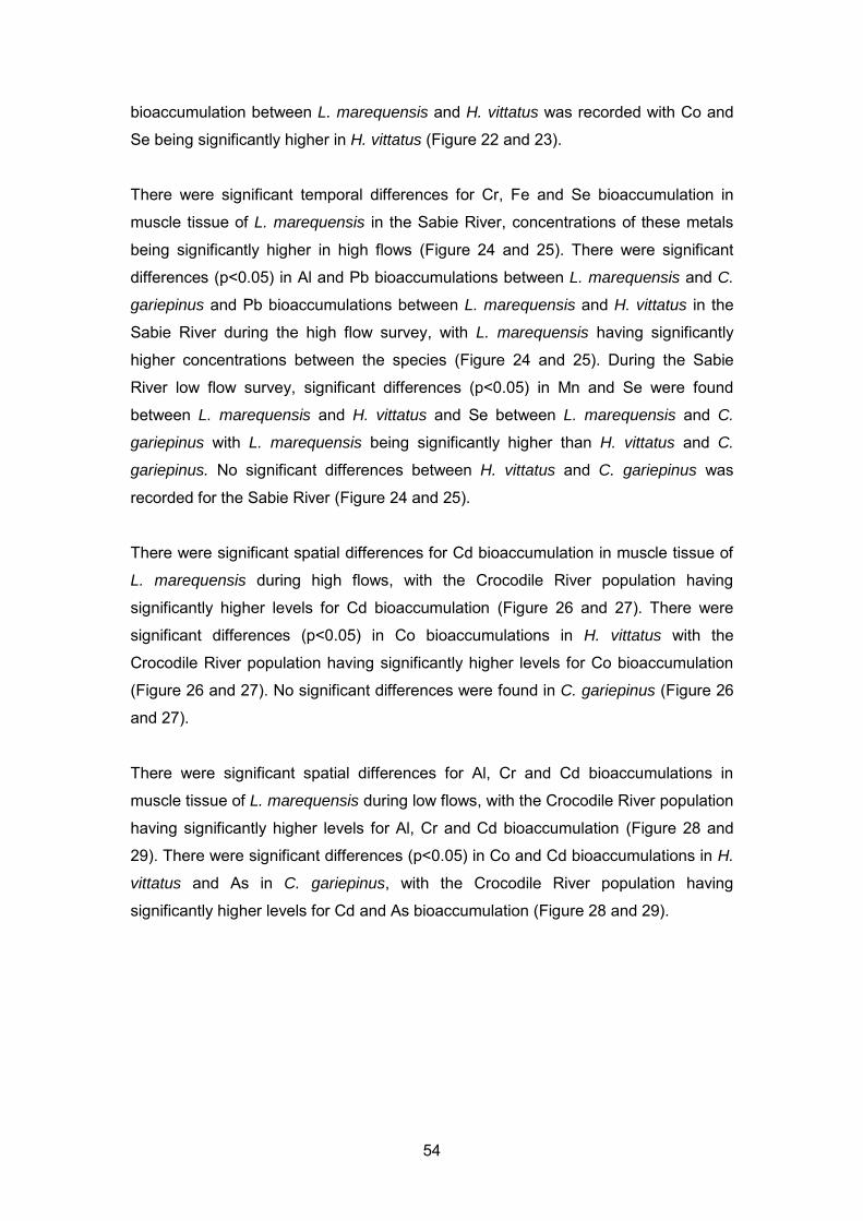
54

bioaccumulation between L. marequensis and H. vittatus was recorded with Co and

Se being significantly higher in H. vittatus (Figure 22 and 23).

There were significant temporal differences for Cr, Fe and Se bioaccumulation in

muscle tissue of L. marequensis in the Sabie River, concentrations of these metals

being significantly higher in high flows (Figure 24 and 25). There were significant

differences (p<0.05) in Al and Pb bioaccumulations between L. marequensis and C.

gariepinus and Pb bioaccumulations between L. marequensis and H. vittatus in the

Sabie River during the high flow survey, with L. marequensis having significantly

higher concentrations between the species (Figure 24 and 25). During the Sabie

River low flow survey, significant differences (p<0.05) in Mn and Se were found

between L. marequensis and H. vittatus and Se between L. marequensis and C.

gariepinus with L. marequensis being significantly higher than H. vittatus and C.

gariepinus. No significant differences between H. vittatus and C. gariepinus was

recorded for the Sabie River (Figure 24 and 25).

There were significant spatial differences for Cd bioaccumulation in muscle tissue of

L. marequensis during high flows, with the Crocodile River population having

significantly higher levels for Cd bioaccumulation (Figure 26 and 27). There were

significant differences (p<0.05) in Co bioaccumulations in H. vittatus with the

Crocodile River population having significantly higher levels for Co bioaccumulation

(Figure 26 and 27). No significant differences were found in C. gariepinus (Figure 26

and 27).

There were significant spatial differences for Al, Cr and Cd bioaccumulations in

muscle tissue of L. marequensis during low flows, with the Crocodile River population

having significantly higher levels for Al, Cr and Cd bioaccumulation (Figure 28 and

29). There were significant differences (p<0.05) in Co and Cd bioaccumulations in H.

vittatus and As in C. gariepinus, with the Crocodile River population having

significantly higher levels for Cd and As bioaccumulation (Figure 28 and 29).

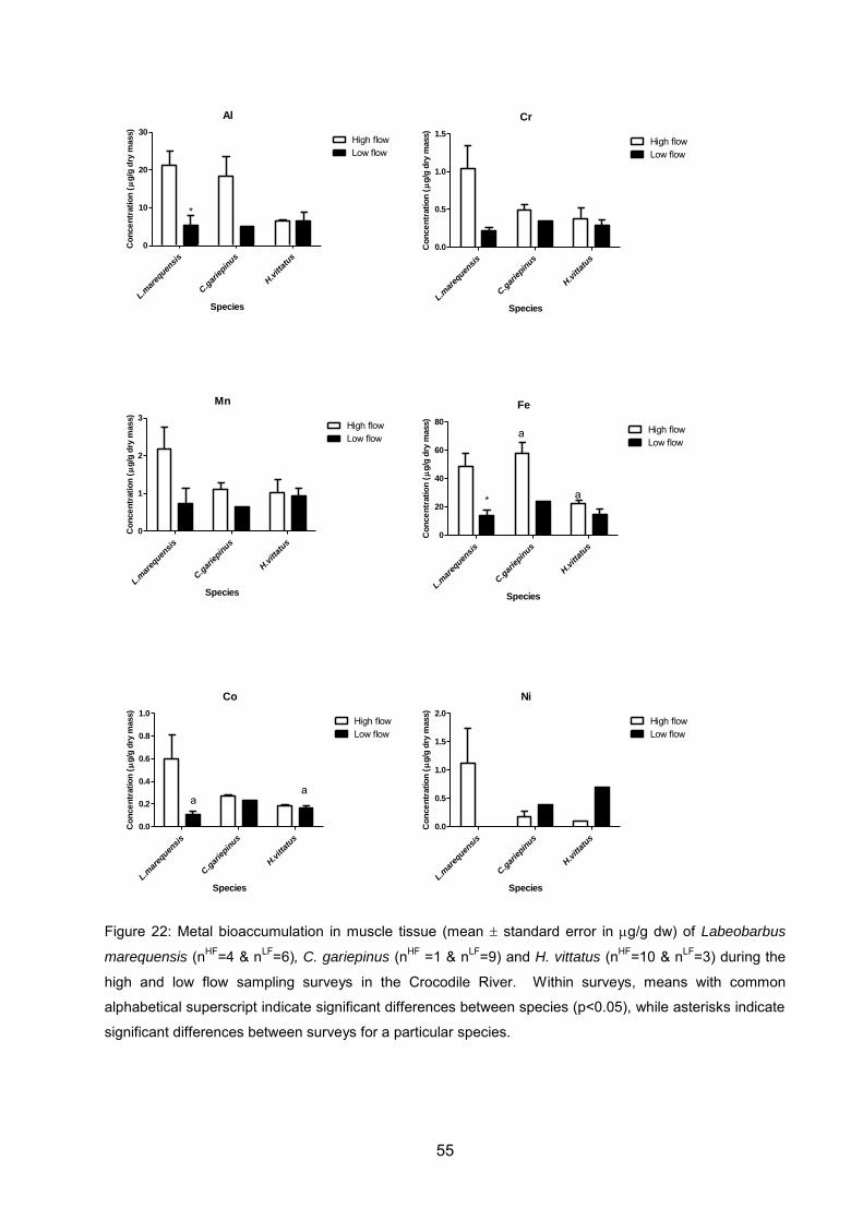
55

Al

L.mar

equen

sis

C.g

arie

pinus

H.v

ittat

us

0

10

20

30High flowLow flow

*

Species

Co

nce

ntr

ati

on

(

g/g

dry

mass)

Cr

L.mar

equen

sis

C.g

arie

pinus

H.v

ittat

us

0.0

0.5

1.0

1.5High flowLow flow

Species

Co

nce

ntr

ati

on

(

g/g

dry

mass)

Mn

L.mar

equen

sis

C.g

arie

pinus

H.v

ittat

us

0

1

2

3High flowLow flow

Species

Co

nce

ntr

ati

on

(

g/g

dry

mass)

Fe

L.mar

equen

sis

C.g

arie

pinus

H.v

ittat

us

0

20

40

60

80High flowLow flow

*

a

a

Species

Co

nce

ntr

ati

on

(

g/g

dry

mass)

Co

L.mar

equen

sis

C.g

arie

pinus

H.v

ittat

us

0.0

0.2

0.4

0.6

0.8


aa

Species

Co

nce

ntr

ati

on

(

g/g

dry

mass)

Ni

L.mar

equen

sis

C.g

arie

pinus

H.v

ittat

us

0.0

0.5

1.0

1.5


Species

Co

nce

ntr

ati

on

(

g/g

dry

mass)

Figure 22: Metal bioaccumulation in muscle tissue (mean standard error in g/g dw) of Labeobarbus

marequensis (nHF=4 & nLF=6), C. gariepinus (nHF =1 & nLF=9) and H. vittatus (nHF=10 & nLF=3) during the

high and low flow sampling surveys in the Crocodile River. Within surveys, means with common

alphabetical superscript indicate significant differences between species (p<0.05), while asterisks indicate

significant differences between surveys for a particular species.

56

Cu

L.mar

equen

sis

C.g

arie

pinus

H.v

ittat

us

0.0

0.5

1.0


Species

Co

nce

ntr

ati

on

(

g/g

dry

mass)

Zn

L.mar

equen

sis

C.g

arie

pinus

H.v

ittat

us

0

20

40

60

80High flowLow flow

*a

a

Species

Co

nce

ntr

ati

on

(

g/g

dry

mass)

As

L.mar

equen

sis

C.g

arie

pinus

H.v

ittat

us

0.0

0.1

0.2

0.3

0.4


*

a

a

Species

Co

nce

ntr

ati

on

(

g/g

dry

mass)

Se

L.mar

equen

sis

C.g

arie

pinus

H.v

ittat

us

0.0

0.2

0.4

0.6

0.8


*

a a

Species

Co

nce

ntr

ati

on

(

g/g

dry

mass)

Cd

L.mar

equen

sis

C.g

arie

pinus

H.v

ittat

us

0.0

0.2

0.4


Species

Co

nce

ntr

ati

on

(

g/g

dry

mass)

Pb

L.mar

equen

sis

C.g

arie

pinus

H.v

ittat

us

0.0

0.5

1.0


Species

Co

nce

ntr

ati

on

(

g/g

dry

mass)



high and low flow sampling surveys in the Crocodile River. Within surveys, means with common

alphabetical superscript indicate significant differences between species (p<0.05), while asterisks indicate

significant differences between surveys for a particular species.

57

Al

L.mar

equen

sis

C.g

arie

pinus

H.v

ittat

us

0

10

20

30

40

50High flowLow flow

aa

Species

Co

nce

ntr

ati

on

(

g/g

dry

mass)

Cr

L.mar

equen

sis

C.g

arie

pinus

H.v

ittat

us

0.0

0.2

0.4


* *

Species

Co

nce

ntr

ati

on

(

g/g

dry

mass)

Mn

L.mar

equen

sis

C.g

arie

pinus

H.v

ittat

us

0.0

0.5

1.0

1.5


a

a

Species

Co

nce

ntr

ati

on

(

g/g

dry

mass)

Fe

L.mar

equen

sis

C.g

arie

pinus

H.v

ittat

us

0

20

40

60

80High flowLow flow

*

Species

Co

nce

ntr

ati

on

(

g/g

dry

mass)

Co

L.mar

equen

sis

C.g

arie

pinus

H.v

ittat

us

0

10

20

30

40

50High flowLow flow

Species

Co

nce

ntr

ati

on

(

g/g

dry

mass)

Ni

L.mar

equen

sis

C.g

arie

pinus

H.v

ittat

us

0.0

0.1

0.2


BDL

Species

Co

nce

ntr

ati

on

(

g/g

dry

mass)



high and low flow sampling surveys in the Sabie River. Within surveys, means with common alphabetical

superscript indicate significant differences between species (p<0.05), while asterisks indicate significant

differences between surveys for a particular species. Below detectable limits is indicated by BDL.

58

Cu

L.mar

equen

sis

C.g

arie

pinus

H.v

ittat

us

0.0

0.5

1.0

1.5


Species

Co

nce

ntr

ati

on

(

g/g

dry

mass)

Zn

L.mar

equen

sis

C.g

arie

pinus

H.v

ittat

us

0

20

40

60

80High flowLow flow

*

Species

Co

nce

ntr

ati

on

(

g/g

dry

mass)

As

L.mar

equen

sis

C.g

arie

pinus

H.v

ittat

us

0.0

0.2

0.4

0.6


Species

Co

nce

ntr

ati

on

(

g/g

dry

mass)

Se

L.mar

equen

sis

C.g

arie

pinus

H.v

ittat

us

0.0

0.2

0.4

0.6


* *ab

ab

Species

Co

nce

ntr

ati

on

(

g/g

dry

mass)

Cd

L.mar

equen

sis

C.g

arie

pinus

H.v

ittat

us

0.00

0.05

0.10

0.15


Species

Co

nce

ntr

ati

on

(

g/g

dry

mass)

Pb

L.mar

equen

sis

C.g

arie

pinus

H.v

ittat

us

0.0

0.1

0.2


a

ab

b

Species

Co

nce

ntr

ati

on

(

g/g

dry

mass)



high and low flow sampling surveys in the Sabie River. Within surveys, means with common alphabetical


differences between surveys for a particular species.

59

Al

L.mar

equen

sis

C.g

arie

pinus

H.v

ittat

us

0

10

20

30

40

50Crocodile RiverSabie River

Species

Co

nce

ntr

ati

on

(

g/g

dry

mass)

Cr

L.mar

equen

sis

C.g

arie

pinus

H.v

ittat

us

0.0

0.1

0.2

0.3

0.4Crocodile RiverSabie River

Species

Co

nce

ntr

ati

on

(

g/g

dry

mass)

Mn

L.mar

equen

sis

C.g

arie

pinus

H.v

ittat

us

0.0

0.5

1.0

1.5


Species

Co

nce

ntr

ati

on

(

g/g

dry

mass)

Fe

L.mar

equen

sis

C.g

arie

pinus

H.v

ittat

us

0

20

40

60


Species

Co

nce

ntr

ati

on

(

g/g

dry

mass)

Co

L.mar

equen

sis

C.g

arie

pinus

H.v

ittat

us

0.0

0.2

0.4

0.6

0.8


*

Species

Co

nce

ntr

ati

on

(

g/g

dry

mass)

Ni

L.mar

equen

sis

C.g

arie

pinus

H.v

ittat

us

0.0

0.5

1.0


BDL BDL

Species

Co

nce

ntr

ati

on

(

g/g

dry

mass)


marequensis (nCR=6 & nSR=6), C. gariepinus (nCR=9 & nSR=4) and H. vittatus (nCR=3 & nSR=9) between the

Crocodile River and Sabie River during low flows. Within surveys, means with common alphabetical



60

Cu

L.mar

equen

sis

C.g

arie

pinus

H.v

ittat

us

0.0

0.2

0.4

0.6


*

Species

Co

nce

ntr

ati

on

(

g/g

dry

mass)

Zn

L.mar

equen

sis

C.g

arie

pinus

H.v

ittat

us

0

20

40

60


*

Species

Co

nce

ntr

ati

on

(

g/g

dry

mass)

As

L.mar

equen

sis

C.g

arie

pinus

H.v

ittat

us

0.0

0.1

0.2

0.3

0.4


*

BDL

Species

Co

nce

ntr

ati

on

(

g/g

dry

mass)

Se

L.mar

equen

sis

C.g

arie

pinus

H.v

ittat

us

0.0

0.2

0.4


*

Species

Co

nce

ntr

ati

on

(

g/g

dry

mass)

Cd

L.mar

equen

sis

C.g

arie

pinus

H.v

ittat

us

0.00

0.05

0.10


*

BDL

Species

Co

nce

ntr

ati

on

(

g/g

dry

mass)

Pb

L.mar

equen

sis

C.g

arie

pinus

H.v

ittat

us

0.0

0.5

1.0


Species

Co

nce

ntr

ati

on

(

g/g

dry

mass)


marequensis (nCR=6 & nSR=6), C. gariepinus (nCR=9 & nSR=4) and H. vittatus (nCR=3 & nSR=9) between the

Crocodile River and Sabie River during low flows. Within surveys, means with common alphabetical



61

Al

L.mar

equen

sis

C.g

arie

pinus

H.v

ittat

us

0

10

20


*

Species

Co

nce

ntr

ati

on

(

g/g

dry

mass)

Cr

L.mar

equen

sis

C.g

arie

pinus

H.v

ittat

us

0.0

0.5

1.0


*

Species

Co

nce

ntr

ati

on

(

g/g

dry

mass)

Mn

L.mar

equen

sis

C.g

arie

pinus

H.v

ittat

us

0

1

2


Species

Co

nce

ntr

ati

on

(

g/g

dry

mass)

Fe

L.mar

equen

sis

C.g

arie

pinus

H.v

ittat

us

0

20

40

60


Species

Co

nce

ntr

ati

on

(

g/g

dry

mass)

Co

L.mar

equen

sis

C.g

arie

pinus

H.v

ittat

us

0.0

0.2

0.4

0.6

0.8


*

Species

Co

nce

ntr

ati

on

(

g/g

dry

mass)

Ni

L.mar

equen

sis

C.g

arie

pinus

H.v

ittat

us

0.0

0.5

1.0

1.5


BDL

Species

Co

nce

ntr

ati

on

(

g/g

dry

mass)


marequensis (nCR=4 & nSR=3), C. gariepinus (nCR=1 & nSR=9) and H. vittatus (nCR=10 & nSR=8) between

the Crocodile River and Sabie River during high flows. Within surveys, means with common alphabetical



62

Cu

L.mar

equen

sis

C.g

arie

pinus

H.v

ittat

us

0.0

0.5

1.0

1.5


*

Species

Co

nce

ntr

ati

on

(

g/g

dry

mass)

Zn

L.mar

equen

sis

C.g

arie

pinus

H.v

ittat

us

0

20

40

60


Species

Co

nce

ntr

ati

on

(

g/g

dry

mass)

As

L.mar

equen

sis

C.g

arie

pinus

H.v

ittat

us

0.0

0.2

0.4

0.6

0.8Crocodile RiverSabie River*

BDL

Species

Co

nce

ntr

ati

on

(

g/g

dry

mass)

Se

L.mar

equen

sis

C.g

arie

pinus

H.v

ittat

us

0.0

0.2

0.4

0.6

0.8


*

Species

Co

nce

ntr

ati

on

(

g/g

dry

mass)

Cd

L.mar

equen

sis

C.g

arie

pinus

H.v

ittat

us

0.0

0.2

0.4


**

Species

Co

nce

ntr

ati

on

(

g/g

dry

mass)

Pb

L.mar

equen

sis

C.g

arie

pinus

H.v

ittat

us

0.0

0.5

1.0


Species

Co

nce

ntr

ati

on

(

g/g

dry

mass)


marequensis (nCR=4 & nSR=3), C. gariepinus (nCR=1 & nSR=9) and H. vittatus (nCR=10 & nSR=8) between

the Crocodile River and Sabie River during high flows. Within surveys, means with common alphabetical


differences between surveys for a particular species.

63

4.4 Discussion

It is well documented that metal bioaccumulation is affected by many factors including species

specific differences (van der Oost et al., 2003). Labeobarbus marequensis, C. gariepinus and H.

vittatus are all at different trophic levels and therefore exposed to different routes of metal

uptake. Labeobarbus marequensis and C. gariepinus are regarded as omnivorous where H.

vittatus are primarily carnivorous, even said to be piscivorous in adults (Bell-Cross, 1965-66;

Skelton, 2001). Labeobarbus marequensis have intestines long enough to characterise them as

herbivorous but are known to eat small invertebrates and fish, although during surveys stomach

content consisted primarily of filamentous algae, they are also regarded as bottom feeders

shifting through cobble and bottom substrate for food (Bell-cross and Minshull, 1988; Fouché,

2009). This could be the reason for the significantly different concentrations of Co, As, Se and

Zn in L. marequensis from the Crocodile River and Al, Mn, Se and Pb in L. marequensis from

the Sabie River when compared to H. vittatus and C. gariepinus.

Metals occur in suspended water and the sediments transported and deposited by water (Dallas

and Day, 2004). Therefore fish exposed to sediment when feeding expose themselves to the

metals within the sediment over and above the metals in the water. Being bottom feeders L.

marequensis could possibly ingest more metals and possibly be exposed to them when feeding

in sediment in relation to C. gariepinus and H. vittatus. Hydrocynus vittatus, which do not feed

near sediment, feed primarily off other fish (Bell-Cross, 1965-66; Skelton, 2001). Clarias

gariepinus are known to be closely related to sediment, often resting and feeding in it, their diet

has high variation to certain food groups and composes primarily of fish, insect, crustaceans,

even plant material (fruits) (Skelton, 2001). Although they eat plant material it is not their primary

diet. Labeobarbus marequensis feed off similar biota yet their diet is not as varied and they feed

primarily off algae, crustaceans and insect larvae found within cobble beds and bottom substrate

(Bell-Cross and Minshull, 1988; Skelton, 2001; Fouché, 2009).

There were differences shown between the different flows within both the Crocodile and Sabie

rivers with bioaccumulation being significantly higher in fish from the high flow surveys when

compared to the low flow surveys. The Crocodile River showed greater variation in this than the

Sabie River in particular to L. marequensis. This could be an indication that surface run-off

washes down metals and exposes them into the system at higher levels. Barker (2006) found

seasonal variation in metals for fish tested in lotic systems. Further physiological state of the fish

may change over season due to certain metals needed for the biological functioning of the

64

species (Falchuk, 1989). Considering that H. vittatus and L. marequensis share similar breeding

periods the difference in metal bioaccumulation could be exposure related (Skelton, 2001;

Fouché, 2009).

For most metals bioaccumulation in muscle of L. marequensis and Cu for H. vittatus was higher

in the Crocodile River than in the Sabie River. For C. gariepinus all metal bioaccumulations

(except Cr) were higher in the Sabie River than in the Crocodile River. Considering that the

Sabie River is regarded as a healthier river to that of the Crocodile River the metal

concentrations for the all three species in the Sabie River can reflect this. (O’Keeffe and Rogers,

2003; DWAF, 2004; Rogers and Luton, 2011). Despite the similar geological compositions

between the two Rivers, the higher impacts on the Crocodile River can be shown in the results

(O’Keeffe and Rogers, 2003; Rogers and Luton, 2011). The Crocodile River is regarded as a

larger anthropogenic impacted river than the Sabie River (O’Keeffe and Rogers, 2003; Rogers

and Luton, 2011).This is reflected in the results for L. marequensis and H. vittatus having higher

metal exposures in the Crocodile River during high flows and low flows this was significant for

metals Al, Cr and Cd and for Cd, during high and low flow conditions respectively. Of interest H.

vittatus showed lower levels of metal concentration than both L. marequensis and C. gariepinus

in both rivers.

Comparisons were made with other known metals concentrations from other systems and fish

species in order to get a guideline to determine the extent of the severity metal accumulations

on the Crocodile River. Prior to this study there have been no metal accumulation studies done

for the Crocodile River. Concentrations for this study were thus compared to other studies

carried out on fish bioaccumulation in other KNP Rivers. Concentrations in L. marequensis from

the Olifants River (Seymore et al., 1995) were found to be lower or similar for Pb (2.9-9.1 g/g

dw) and Mn (7-35.5 g/g dw). Comparisons to the results by Barker (2006) who studied metal

bioaccumulation in whole species of L. marequensis revealed lower and in some cases similar

concentrations for Al (13.0-663.0 g/g dw), Cd (0.1-2.8 g/g dw), Mn (5.2-75.0 g/g dw), Ni (0.1-

12 g/g dw), Fe (0.5-754.4 g/g dw), Pb (0.4-26.0 g/g dw), Cr (0.1-19.9 g/g dw), Cu (0.1-208

g/g dw) and Zn (20.2-134.8 g/g dw)

When results of this study are compared to metal bioaccumulation in muscle tissue of the

Orange River mudfish, Labeo capensis from the known contaminated Vaal River (Wepener et

al., 2011) concentrations were found again to be similar or higher for Pb (0.025-0.067 g/g dw),

Zn (13.1-18.46 g/g dw), Cr (0.142-0.261 g/g dw). The concentrations of Ni (0.187-0.517 g/g

dw) and Cu (1.78-14.3 g/g dw) were lower than in the fish muscle from the Vaal River. Gutleb

et al. (2002) conducted a baseline study for a rain forest fed river in Peru before oil mining was

65

started and metal bioaccumulation results from this study were higher for Fe, Co, Zn, As, Se, Cd

and Pb; Fe (.071-0.157 g/g dw), Co (0.017-0.127 g/g dw), Zn (23.75-27.02 g/g dw), As

(0.015-0.101 g/g dw), Se (0.070-0.142 g/g dw), Cd (0.010-.071 g/g dw), Pb (0.091-0.441

g/g dw) with the exception of Cu (1.62-4.12 g/g dw), Mn (2.91-20.75 g/g dw) and Ni (0.240-

0.943 g/g dw).

Compared to regions with known high metal bioaccumulation, e.g. a study in Rwanda by

Sekomo et al. (2011) concentrations were found to be higher in Zn (5.11 g/g dw) for this study.

While Cd (2.85 g/g dw) during the high flow in the Crocodile River was higher than the

respective other flows and species tested. Bervoets and Blust (2002) tested for metal

concentrations in fish along a Cd and Zn pollution gradient in a Belgian River system. Results

from this study in L. marequensis were similar to levels for Zn (40-45 g/g dw, while in this study

= 39-49 g/g dw) in the highly polluted Belgian site. In a later study by Reynders et al. (2008) for

the same Belgian sites metal concentrations were found above the levels in this study for Cu (2-

3 g/g dw), Zn (30-60 g/g dw) but below for Cd, which was below detectable limits.

Zinc concentrations within the Crocodile River for the population of L. marequensis were similar

or higher in concentration than in other river systems (Seymore et al., 1995; Barker, 2006;

Wepener et al., 2011). Zinc however is crucial for the development of eggs and gets stored in

storage tissue until eggs are fertilized (Falchuk, 1998). This is relevant for female fish; the male

to female ratio in this study was 6:1, possibly indicating the moderate levels of Zn in the study.

This does not indicate why all the other metals are slightly elevated in L. marequensis for the

Crocodile River. Metal concentrations being similar and in cases higher for this study in relation

to other studies raises concern for the population of L. marequensis in the Crocodile River as

metal levels are significantly higher than that of H. vittatus and C. gariepinus and than the

population within the Sabie River, showing that despite having similar to above normal metal

concentration they are being more effected by metals than other species and than in other river

systems.

4.5 Conclusion

With significantly (p>0.05) higher metal bioaccumulation in L. marequensis from Crocodile River

than the Sabie River, it does raise concerns with regards to the potential influence it may have

on this river’s population. This could possibly be compounded with other stress factors which

can cause the overall decline in the L. marequensis population on the Crocodile River. Metals

66

that were consistently higher in L. marequensis were Zn and Pb. Zinc, in particular when

compared to other studies, showed that levels were similar or slightly elevated in this study than

to other polluted sites. However high bioaccumulation due to Zn storage for the development of

eggs needs to be considered and could be the reason for the high concentration of Zn. The

sample did obtain more male L. marequensis than females, the ratio of male to female (6:1)

presenting moderate levels of Zn in the results, as females had high levels ( 90 g/g dw) while

males had low levels ( 15 g/g dw) of Zn concentrations.

Possible sources of metal pollution in the Crocodile River can be from a number of industrial

sectors in the Nelspruit area, gold mines towards Barberton and the magnetite mine near the

town of Malelane (DWAF 2004; Rogers and Luton, 2011). With the increases in water usage

and demand from various sectors, there is a concern as to the use and industrial effluent run-off

further impacting on the Crocodile River (Rogers and Luton, 2011). This study has indicated that

the population of L. marequensis in the Crocodile River has elevated levels of metals Pb, Zn and

Cd although the metal bioaccumulations are not at concerning levels yet.

67

5 CHAPTER 5: GENERAL CONCLUSION AND MANAGEMENT RECOMMENDATIONS.

5.1 General conclusions

The aims of the study were to evaluate the current health, habitat use and movement of L.

marequensis and other fishes in the Crocodile River, KNP. To reach the aims a behavioural and

ecotoxicology assessment of the population of L. marequensis in the Crocodile River was

undertaken and the hypothesis then accepted or rejected.

In consideration to the first hypothesis which states; Labeobarbus marequensis make use of

defined home ranges on a reach scale (<10 km) and behave differently during different seasons

and times of day, the outcomes of the study allow for the hypothesis to be accepted. Large L.

marequensis do make use of defined home ranges on a reach scale which is restricted to less

than 10 km it was further found that the home ranges are smaller and found to be <5 km. Large

L. marequensis do behave differently during different seasons, during the summer showing the

greater difference in behaviour. Behaviour of Labeobarbus marequensis change during the

course of the day, TOD showed the species to a diurnal species. The study showed that these

large L. marequensis do not take part in seasonal migrations, instead remained in a home range

surrounding the focal area of the study. This shows the importance of these habitats within the

Crocodile River. These habitat preferences are unique to only a few stretches of the Crocodile

River. Therefore it is of importance to the conservation of the species that these habitats are

maintained and protected.

Furthermore in consideration of the second hypothesis which states; the movement of L.

marequensis decreases when flows increase rapidly in the Crocodile River. This hypothesis was

accepted, the movement of L. marequensis decreases significantly when flows in the Crocodile

River increase rapidly from 10 m3.s-1 to 60 m3.s-1. Flows play an important role in change and

availability of habitat types. The response to flow changes indicated that during extreme high

and erratic flows L. marequensis would decrease their movements and wait for low to moderate

and consistent flows. Combining flow and seasonal response showed that flows are important

during the spring period and the two together can be some form of cue to the heightened activity

during consistent low to moderate flows and spring. The importance of more natural flows

should be fed into management policies and programs to regulate the flow (discharge) from dam

releases and extractions to better suite L. marequensis. Considering L. marequensis do better in

constant, stable flows the irregular discharges caused by impoundments may cause a river to be

in a high unstable flux longer than it should be naturally. Therefore a more natural discharge will

bring back stability into the aquatic river system minimising high extended unfavourable flows.

68

In considering the third hypothesis which states; the levels of metals in L. marequensis in the

Crocodile River are greater than H. vittatus and C. gariepinus from the Crocodile and Sabie

Rivers was accepted. Metal bioaccumulations in the study showed significant differences in

concentration between the Crocodile River and the Sabie River populations of L. marequensis.

The same spatial differences were also found for H. vittatus and C. gariepinus. Further

significant differences were found between the different species indicating different routes of

metal exposure and/or ability to metabolize following uptake between the three species. Overall

however L. marequensis had higher metal concentrations than the other two species. The

higher metal bioaccumulation in the fish from the Crocodile River than in the Sabie River was

expected due to levels of activity in the respective catchments. This could indicate that the

population within the Crocodile River is under more stress than that in the Sabie River. The

second part to the hypotheses stating that the metal concentrations negatively affect the L.

marequensis population in the Crocodile River is inconclusive. The comparisons made with

bioaccumulation in fish from known heavily polluted rivers and this study is still of no concern as

yet, however the increased pressure from human activity on the Crocodile River may cause

these concentrations to worsen over time.

5.2 Management recommendations

There are management plans and policies in place to better manage the greater Nkomati River

systems, of which the Crocodile River falls under. The Interim IncoMaputo Agreement (IIMA)

between Swaziland, South Africa and Mozambique is internationally important in providing

Mozambique with enough water to sustain the urban growth of Maputo (DWAF,2004; Rogers

and Luton, 2011). These plans and policies are managed using existing models and information

which may not always be true indications to what is happening in the environment and because

of this it is crucial to continue with findings to better these management plans and policies as in

the adaptive management approach by KNP (Roger and O’Keeffe, 2003). Therefore the

evaluation of implementing management plans and policies can be re-incorporated into

management ending in a better use of the river system in the long term. This study was able to

indicate the importance of flow (discharge) and time of day on the behavioural response of L.

marequensis and the importance of maintaining the preferred habitat for the species to ensure

its survival. Discharge in river management is always of importance as it alters downstream

available habitats (Dallas and Day, 2004). Constant flow allows the river to stabilize creating

preferred habitats to be around for longer periods, this is not to distract from natural flows yet to

enforce natural flows and not allow the release of water at irregular intervals outside the natural

69

discharge caused by seasonal rains. The importance of spring to L. marequensis behaviour

indicates the value of natural flows during that period to allow for availability of spawning events.

The bio-accumulation of metals in tested fish is concerning and minimizing the effluent of heavy

metal wastes into the Crocodile River system is important to the survival of L. marequensis and

should be mitigated where ever possible.

Further studies are needed to better understand the spawning habits of L. marequensis and the

associated cues in particular to the day length, flows and associated spawning habitat. This

study has gained more knowledge on the response of L. marequensis to discharge. Further

studies on this topic will help fine tune the understanding that discharge has to concerned fish

species, such as L. marequensis, assessing in the better management of impoundments to

replicate natural discharges or discharges better suited the survival of fish. Current telemetry

techniques can assist greatly in these studies. Since L. marequensis bioaccumulated the

highest levels of metals it is recommended that the species be used as indicator species when

testing for heavy metals. Future studies should be aimed at linking the metal exposure (in the

form of bioaccumulation) with their effects on ecology and biology of organisms, e.g. using

biomarkers with behaviour to find effects of metals on behaviour of fish.

70

6 CHAPTER 6: REFERENCES

Angliss M.K., Fouché P.J., Rodgers S.S.M. Vlok W. 2005. A biomonitoring survey of the Olifants River

Catchment falling within the Limpopo Province: Field survey of 2004. Technical report of the

Limpopo Environmental Affairs Department.

Barker H.J. 2006. (unpub.) Physico-chemical caharacteristics and metal bioaccumulation in four major

river systems that transect the Kruger National Park, South Africa. Unpub. M.Sc Thesis,

University Johannesburg. Auckland Park, Johannesburg

Bell-Cross G. 1965-66. Preliminary observations on Hydrocynus vittatus in the upper Zambezi River

System. Fish. Res. Bull. Zambia (1965-66), 4:119

Bell-Cross G. and Minshull J.L. 1988. The fishes of Zimbabwe. National Museums and Monuments of Zimbabwe, Harare, 294 pp.

Bervoets L. and Blust R. 2002. Metal concentrations in water, sediment and gudgeon (gobio gobio)

from a pollution gradient: relationship with fish condition factor. Env. Pollut. 126 2003:9-19.

Brand M., Maina J., Mander M. and O’ Brien G. 2009. Characterisation of the social and economic

value of the use and associated conservation of the yellowfishes in the Vaal River. WRC report

KV 226/09. Water research Commission. Pretoria.

Burnham KP, Anderson DR. 1998. Model selection and inference: a practical information-theoretic

approach. New York: Springer-Verlag.

Chapman P.M. 1997. Is bioaccumulation useful for predicting impacts? Mar. Pollut. Bull. 34 5:282-283.

Cooke S.J. and Schreer J.F. 2003. Environmental monitoring using physiological telemetry: A case

study examining common carp responses to thermal pollution in a coral fired generation station

effluent. Water, Air and Soil Pollution: 142:113-136

Cooke S.J., Hinch S.G., Wikelski M., Andrews R.D., Kuchel L.J., Wolcott T.G. and Butler P.J. 2004.

Biotelemetry: a mechanistic approach to ecology. Trends in Ecology and evolution. 19(6) June

2004.

71

Crass R.S. 1964. Freshwater Fishes of Natal. Shuter & Shooter, Pietermaritzburg.

Crook D.A. 2004. A method for externally attaching radio transmitters to minimize dermal irritation.

Journal of fish biology 2004 64:258-261

Dallas H.F. and Day J. A. 2004. The effect of water quality variables on aquatic ecosystems: A review.

WRC Report No. TT224/04, Water Research Commission, Pretoria.

Department of Water affairs and Forestry (DWAF) 1995. Crocodile River catchment, eastern Transvaal:

Water quality assessment. Vol. 1-9, DWAF, Pretoria. IN: Hills L., Vos P., Moolman J. and

Silberbauer M. 2001. Inventory of River Health Programme monitoring sites on the Olifants,

Sabie and Crocodile Rivers. WRC Report No:. 850/2/01. Water Research Commission, Pretoria.

Department of Water affairs and Forestry (DWAF) 2002. National Water Resource Strategy. Proposed

first edition. DWAF, Pretoria 132pp

Department of Water affairs and Forestry (DWAF) 2004. Internal Strategic perspective: Inkomati water

management area. DWAF Report No: P WMA 05/000/00/0303 DWAF, Pretoria.

De Villiers P. and Ellender B. 2008a. Status of the Orange-vaal largemouth, Labeobarbus aeneus

(Burchell, 1822). IN: Impson N.D., Bills, I.R. and Wolhuter L. 2008. Technical Report on the

state of Yellowfishes in South Africa 2007. WRC Report KV212/08. Water Research Commision.

Pretoria.

De Villiers P. and Ellender B. 2008b. Status of the Orange-vaal smallmouth, Labeobarbus

kimberleyensis (Gilchrist and Thompson, 1913). IN: Impson N.D. Bills, I.R. and Wolhuter L.

2008. Technical Report on the state of Yellowfishes in South Africa 2007. WRC Report

KV212/08. Water Research Commision. Pretoria.

Dodson J.J. 1997. Fish migration, an evolutionary perspective. IN: Godin JG.J. 1997. Behavioural

ecology of teleost fishes. Oxford University Press.

Driver A., Maze K., Rouget M., Lombard A.T., Nel J., Turpie J.K., Cowling R.M., Desmet P., Goodman

P., Harris J., Jonas Z., Reyers B., Sink K. and Strauss T. 2005. National Spatial Biodiversity

Assessment 2004: priorities for biodiversity conservation in South Africa. Strelitzia, 17. South

African National Biodiversity Institute, Pretoria. IN: Rivers-Moore N.A. 2011. Deriving

72

conservation targets for rivers. WRC report No. 1796/1/10. Water Research Commission,

Pretoria.

Du Preez H.H. and Steyn G.J. 1992. A preliminary investigation of the concentration of selected metals

in the tissues and organs of the tigerfish (Hydrocynus vittatus) from the Olifants River, Kruger

National Park, South Africa. Water SA 1992:18 0704

Ellender, B.R. 2008. The impact of angling on Smallmouth and Largemouth yellowfish, Labeobarbus

aeneus and Labeobarbus kimberleyensis, in lake Gariep, South Africa. Unpublished Masters of

Science Thesis. Rhodes University. Grahamstown. IN: O’Brien, G. and De Villiers, P. 2010.

Aspects of the biology and ecology of the orange-vaal largemouth and smallmouth yellowfish in

the Vaal River. WRC Report. Water Research Commission, Pretoria.

Falchuk K. H., 1998. The molecular basis for the role of zinc in developmental biology. Mol. and Cell.

Biochem. 188: 41-48,

Fouché P.S.O., 2009 (unpub.). Aspects of the ecology and biology of Lowveld Large-scale Yellowfish

(Labeobarbus marequensis Smith, 1843) in the Luvhuvhu, Limpopo River System. South Africa.

Unpub. PhD Thesis, Department of Biodiversity (Zoology), School of Molecular and Life

Sciences, Faculty of Science and Agriculture,University of Limpopo – Turfloop campus.

Fouché P.S.O. and Gaigher I.G. 2001. Niche differentiation in the rheophilic fishes of the Mutshindudi

River. IN: Gaigher I. G., (Editor). A Socio-biological study of the aquatic resources and their

utilisation in an underdeveloped rural region, the Mutshindudi River Catchment. WRC Project

Report 714/3/01, Water Research Commission, Pretoria.

Fouché P.S.O., Angliss M.K. and Vlok W., 2005. The utilization of the Xikundu fishway by Labeobarbus

marequensis. Proceedings of the 9th Yellowfish Working Group conference. IN: Fouché P.S.O.

(2009) Aspects of the ecology and biology of Lowveld Large-scale Yellowfish (Labeobarbus

marequensis Smith, 1843) in the Luvhuvhu, Limpopo River System. South Africa. PhD Thesis,

University of Limpopo.

Gaigher I.G. 1969. Aspekte met betrekking tot die Ekologie, Geografie en Taksonomie van

Varswatervisse in die Limpopo- en Incomatiriviersisteem. Unpublished Ph.D. Thesis, Rand

Afrikaans University.

73

Godfrey L. 2002 Ecological Reserve Determination for the Crocodile River Catchment, Incomati

System, Mpumalanga. Technical Report for the Department of Water Affairs and Forestry, by

the Division of the Environment and Forestry Technology, Report No. ENV-P-C 2002-009.

CSIR, Pretoria.

Godin JG.J., 1997. Behavioural ecology of teleost fishes. Oxford University Press.

Gutleb A. C., Helsberg A. and Mitchell C. 2002. Heavy metal concentration in fish from a pristine

rainforest valley in Peru: A baseline study before the start of Oil-drilling activities. Bull. Environ.

Contam. Toxicol. (2002) 69:523-529

Heath R.G.M. and Claassen M. 1999. An overview of the Pesticide and Metal levels present in

populations of the larger indigenous fish species of selected South African rivers. WRC report

No. 428/1/99. Water Research Commission. Pretoria.

Hills L., Vos P., Moolman J. and Silberbauer M. 2001. Inventory of River Health Programme monitoring

sites on the Olifants, Sabie and Crocodile Rivers. WRC Report No:. 850/2/01. Water Research

Commission, Pretoria.

Hirschowitz P.M., Birkhead A.L. and James C.S. 2007. Hydraulic modelling for ecological studies for

South African Rivers. WRC Report no: K5/105. Water Research commission. Pretoria.

Hodder H.K., Masters J.E.G., Beaumont W.R.C., Gozlan R.E., Pinder A.C. Knight C.M. and Kenward

R.E. 2007. Techniques for evaluating the spatial behaviour of river fish. Hydrobiologia (2007)

582:257-269

Impson N.D., Bills I.R. and Wolhuter L. 2008. Technical Report on the state of Yellowfishes in South

Africa 2007. WRC Report KV212/08. Water Research Commision. Pretoria.

IUCN Red Data List. 2007. http://www.iucnredlist.org/search/details.php/2560/summ

Jackson P.B.N., 1961. The Fishes of Northern Rhodesia, a Checklist of Indigenous Species. The

government Printer, Lusaka. 140pp

Jepsen N, Koed A, Thorstad EB and Baras E., 2002 Surgical implantation of telemetry transmitters in

fish: how much have we learned? Hydrobiologia 165: 241-250.

http://www.iucnredlist.org/search/details.php/2560/summ

74

Johnson J.H. 1957. Sonic tracking of adult salmon at Bonneville Dam. U.S. Department of the Interior,

Fisheries Bulletin: 176 60:471-485

Jubb R.A. 1967. Freshwater Fishes of Southern Africa. A.A. Balkema, Cape Town.

Kleynhans C. J. 1991. Voorlopige riglyne vir die klassifisering van die Transvaalse vissorte in

sencietiwiteitsklasse. Transvaalse Hoofdirektoraat Natuur en Omgewingsbewaring,

Werkswinkel, Skukuza.

Kleynhans C.J. 1997. An exploratory investigation of the instream biological integrity of the Crocodile

River, Mpumualanga, as based on the assessment of fish communities. Internal Report. Institute

for water Quality Studies, Department of Water Affairs and Forestry, South Africa. IN: Hills L.,

Vos P., Moolman J. and Silberbauer M. 2001. Inventory of River Health Programme monitoring

sites on the Olifants, Sabie and Crocodile Rivers. WRC Report No:. 850/2/01. Water Research


Kleynhans C.J. 1999. The development of a fish index to assess the biological integrity of South African

rivers. Water SA 25 (3).

Kleynhans C.J., Schulz G.W., Engelbrecht J.S. and Rousseau F.J. 1992. The impact of a paper mill

effluent spill on the fish populations of Elands and Crocodile Rivers (Incomati System,

Transvaal). ISSN 0378-4738 Water SA 18(2)

Koehn J.D. 2000. Why use radio tags to study freshwater fish?. In: Hancock, DA, Smith D, Koehn JD,

editors. Fish Movement and Migration. Sydney: Australian Society for Fish Biology.

Kramer D.L., Rangeley R.W. and Chapman, L.J. 1997. Habitat Selection: patterns of spatial distribution

from behavioural decisions. IN: Godin JG.J. ed. 1997. Behavioural ecology of teleost fishes.

Oxford University Press.

Littell RC, Milliken GA, Stroup WW, Wolfinger RD. 1996. SAS system for mixed models. North Carolina:

SAS Institute, Cary.

Leslie B. J. 2007. Thresholds of Potential Concern for Large Scale Yellow Fish, a Project in the

Crocodile River, KNP. Abstract in Yellow Fish Working Group newsletter, 2007.

75

Lucas M.C. and Baras E. 2000. Methods for study freshwater fish in the natural environment. Fish and

Fisheries, 2000, 1, 283-316

Mabunda D., Pienaar D.J., Verhoef J. 2003. The Kruger National Park: A century of management and

research. IN: Du Toit J.T., Rogers K.H., Biggs H. 2003. The Kruger Experience, ecologay and

management of savanna heterogeneity. Island Press pp3

Marx H.M. and Avenant-Oldewage A., 1998. A further investigation into the bioaccumulation of lead and

zinc in the organs and tissues of the African sharptooth catfish, Clarias gariepinus from two

localities in the Olifants River, Kruger National Park. Koedoe 41:2

Nel J.L., Roux D.J., Maree G., Kleynhans C.J., Moolman J., Reyers B., Rouget M. and Cowling R.M.

2007 Rivers in peril inside and outside protected areas: a systematic approach to conservation

assessment of river ecosystems. Diversity and Distributions, 13, 341-352. IN: Rivers-Moore N.A.

2011. Deriving conservation targets for rivers. WRC report No. 1796/1/10. Water Research


Nikolsky G.V. 1963. The Ecology of Fishes. Academic Press, New York. 351pp IN: IN Fouche P.S.O.

2009. Aspects of the ecology and biology of Lowveld Large-scale Yellowfish (Labeobarbus

marequensis Smith, 1843) in the Luvhuvhu, Limpopo River System. South Africa. PhD Thesis,

University of Limpopo.

O’Brien G. and De Villiers P. 2011. Aspects of the biology and ecology of the orange-vaal largemouth

and smallmouth yellowfish in the Vaal River. WRC report No. TT508/11. Water Research


O’Brien G., Nel L., De Villers P., Jacobs F. and Hoffman A. 2012. Home ranges, habitat use, migrations

and general behaviour. IN: O’Brien G. and De Villiers P. 2011. Aspects of the biology and

ecology of the orange-vaal largemouth and smallmouth yellowfish in the Vaal River. WRC

Report. Water Research Commission, Pretoria.

O’Brien G., Bulfin J.B., Husted A., Smit, N.J. 2012. Comparative behavioural assessment of an

established and a new tigerfish (Hydrocynus vittatus) population in two man-made lakes in the

Limpopo River catchment; southern Africa. African Journal of Aquatic Science 2012, 37 (3).

Oellerman L.K. and Skelton P.H. 1989. Hexaploidy in yellowfish species (Barbus, Pisces, Cyprinidae)

from Southern Africa. J. Fish Biol. 37: 105-115. IN Fouché P.S.O. 2009. Aspects of the ecology

76

and biology of Lowveld Large-scale Yellowfish (Labeobarbus marequensis, Smith 1843) in the

Luvhuvhu, Limpopo River System. South Africa. PhD Thesis, University of Limpopo.

O’Keeffe J. and Rogers K.H. 2003. Heterogeneity and management of the Lowveld Rivers. IN: Du Toit

J. T., Rogers K.H. and Biggs H.C. 2003. The Kruger Experience, ecology and management of

savanna heterogeneity. Island press pp447

Økland F, Hay CJ, Næsje TF, Nickandor N, Thorstad EB. 2003. Learning from unsuccessful radio

tagging of common carp in a Namibian reservoir. J Fish Biol, 62: 735-739.

kland F., Thorstad E.B., Hay C.J., Naesje T.F., Chanda B. 2005. Patterns of movement and habitat

use by tigerfish (Hydrocynus vittatus) in the Upper Zambezi River (Namibia). Ecology of

Freshwater fish 14:76-86

Paxton B.R. 2004a. Catchment-wide movement patterns and habitat utilisation of freshwater fish in

rivers: implications for dam location, design and operation, a review and methods development

for South Africa. WRC Report No. KV145/04. Water Research Commission, Pretoria.

Paxton B.R. 2004b. Tracking movement of large fish species through a river system: Methods

Development. WRC Report No. KV 157/04. Water Research Commission, Pretoria.

Pienaar U. de V. 1978. The Freshwater fishes of the Kruger National Park. Sigma Press. Pretoria. 91pp

Pollard S.R., Weeks D.C. & Fourie A. 1996. A pre-impoundment study of the Sabie-Sand River system,

Mpumalanga with special reference to predicted impacts on the Kruger National Park. Vol. Two:

Effects of the 1992 drought on the fish and macro-invertebrate fauna. WRC Report No.

294/2/96. Water Research Commission. Pretoria.

Rainbow P.S. 2007. Trace metal concentrations in aquatic invertebrates: why and so what? Environ.

Pollut. 120: 497-507.

Reynders H., Bervoets L., Gelders M., De Coen W.M. and Blust R. 2008. Accumulations and effects of

metals in caged carp and resident roach along a metal pollution gradient. Science of the Total

Environment 391 2008: 82-95.

Resh V.H., Brown A.V., Kovich A.P., Gurtz M.E., Li H.W., Minshal W. Reice S.R., Sheldon A.L.,

Wallace J.B. and Wissmar R.C. 1988. The role of disturbance in stream ecology. Journal of the

77

North American Benthic Society 7:433-455. IN O’Keeffe J. and Rogers K.H. 2003. Heterogeneity

and management of the Lowveld Rivers. IN: Du Toit J. T., Rogers K.H. and Biggs H.C. 2003.

The Kruger Experience, ecology and management of savanna heterogeneity. Island press

pp447

Rivers-Moore N.A. 2011. Deriving conservation targets for rivers. WRC report No. 1796/1/10. Water

Research Commission, Pretoria.

Rogers K. H. and O’Keeffe J. 2003. River Heterogeneity: ecosystem structure, function and

management. IN: Du Toit J. T., Rogers K.H. and Biggs H.C. 2003. The Kruger Experience,

ecology and management of savanna heterogeneity. Island press pp189

Rogers K. R. and Luton R. 2011. A strategic adaptive management as a framework for implementing

integrated water resource management in South Africa. WRC Report No. KV 245/10. Water

Research Commission, Pretoria

Rogers R.B. and White G.C. 2002. Analysis of movement and habitat use from telemetry data. IN:

Brown, M and Guy, C., ed. 2007. Analysis and interpretation of freshwater fisheries data.

American Fisheries Society, Bethesda, Maryland: 625-676

Russell I.A. and Rodgers K.H. 1989. The distribution and composition of fish communities in the major

rivers of the Kruger National Park. In: S. Kienzle and H. Maaren (Editors). Proceedings of the

Fourth South African National Hydrological Symposium, University of Pretoria, Pretoria. 28-288.

IN: Impson N.D., Bills, I.R. & Wolhuter L. 2008. Technical Report on the state of Yellowfishes in

South Africa 2007. WRC Report KV212/08. Water Research Commision. Pretoria.

Russell I.A. 1997. Monitoring the conservation status and diversity of fish assemblages in the major

rivers of the Kruger National Park. Unpublished Ph.D. Thesis, University of the Witwatersrand,

Johannesburg.

Schiemer 2000. Fish as an indication for the assessment of the ecological integrity of large rivers.

Hydrobiologia. 422-423. (0): 271-278.

Sekomo C. B., Nkuranga E., Rousseau D.P.L. and Lens P.N.L. 2011. Fate of metals in an urban

natural wetland: The Nyabugog Swamp (Rwanda). DOI 10.1007/s11270-010-0426-9. Water Air

Soil Pollut. (2011) 214:321-333

78

Seymore T., Du Preez H.H., Van Vuren J.H.J. 1995. Manganese, lead and strontium bioaccumulation in

the tissues of the yellfish, Barbus marequensis from the lower olifants River, Eastern Transvaal.

Water SA 21( 2)

Skelton P.H. 2000. Flagships and fragments – perspective on the conservation of freshwater fishes in

Southern Africa. African Journal of Aquatic Science, 25(1), 37- 42.

Skelton P.H. 2001. A Complete Guide to the Freshwater Fishes of Southern Africa, 2nd Edition. Struik

Publishers, Cape Town. pp395.

Skelton P.H. and Bills I.R. 2008. An introduction to Yellowfish and the report. IN: Impson N.D., Bills I.R.

and Wolhuter L. 2008. Technical Report on the state of Yellowfishes in South Africa 2007. WRC

Report KV212/08. Water Research Commission. Pretoria.

Smith A. 1841. Pisces. In : illustrations of zoology of South Africa; consisting Chiefly of figures and

descriptions of the objects of natural history collected during an expedition into the interior of

South Africa in 1834-36. Illust. Zool. S. Africa 4:1-31.

Stephen D.W. and Krebs J.R. 1986. Foraging theory. Princton University Press, Princeton. IN: Kramer

D.L., Rangeley R.W. and Chapman L.J. 1997. Habitat Selection: patterns of spatial distribution

from behavioural decisions. IN: Godin JG.J. ed. 1997. Behavioural ecology of teleost fishes.

Oxford University Press.

Steyn P. 1982. Birds of Prey of Southern Africa. David Phillip, Cape Town, South Africa. 309pp.

Thorstad E.B., Hay C.J., Naesje T.F. and Økland F. 2001. Movements and habitat utilisation of three

cichlid species in the Zambezi River, Namibia. Ecology of Freshwater Fish 10:238-246.

Thorstad E.B., Hay C.J., Næsje T.F., Chanda B. and Økland F. 2004. Space use and habitat utilisation

of tigerfish and the two cichlid species nembwe and threespot tilapia in the Upper Zambezi

River. Implications for fisheries management. – NINA Norwegian Inatitute for Natural Research

Project Report 24. 23.

Tomschy H., Husted A., O’Brien G., Cloete Y., van Dyk C., Pieterse G.M., Wepener V., Nel A.,

Reisinger U. 2009. Environmental study to establish the baseline biological and physical

conditions of the Letsibogo dam near Selebi Phikwe, Botswana. European Union’s 8th EDF

79

(European Development Fund) Programme: Economics Diversification of the Mining Sector, 8 ACP BT

13.

Townsend C.R. 1989. The patch dynamics concept of stream community ecology. Journal of the North

America Benthic Society 8:36-50. IN: O’Keeffe, J. and Rogers K.H. 2003. Heterogeneity and

management of the Lowveld Rivers. IN: Du Toit J. T., Rogers K.H. and Biggs H.C. 2003. The

Kruger Experience, ecology and management of savanna heterogeneity. Island press pp447

Trefehten R.S. 1956. Sonic equipment, for tracking individual fish. U.S. Fish and wildlife Service,

Special Scientific Report-Fisheries No. 19. 11

Van der Oost R., Beyer J. and Vermeulen N.P.E., 2003. Fish Bioaccumulation and biomarkers in

environmental risk assessment: a review. Environ. Toxicol. Pharmacol. 13, 57-149

Van Vuren J.H.J., Du Preez H.H. and Deacon A.R. 1994. Effects of pollutants on the physiology of fish

in the Olifants River (Eastern Transvaal). WRC Report 350/1/94. Water Research Commission.

Pretoria.

Vidal L.B. 2008. Fish as ecological indicators in Mediterranean freshwater ecosystems. PhD Thesis.

University of Girona, Spain.

Vlok W. 1992. Die testisultrastruktuur van Cyprinidae in Suid Afrika en Israel met spesiale verwysing na

kriobewaring van Barbus aeneus sperme. Unpublished Thesis, Randse Afrikaanse Universiteit,

Johannesburg. IN: Fouché P.S.O. (2009) Aspects of the ecology and biology of Lowveld Large-

scale Yellowfish (Labeobarbus marequensis, Smith 1843) in the Luvhuvhu, Limpopo River

System. South Africa. PhD Thesis, University of Limpopo.

Wepener V., van Dyk C., Bervoets L., O’BrienG., Covaci A. and Cloete Y., 2011. An assessment of the

influence of multiple stressors on the Vaal River, South Africa. Physical and Chemistry of the

Earth. 36 2011:949-962

Zar J.H. 1996. Biostatistical analysis 3rd ed. Prentence-Hall International INC., N.J. 662

80

7 CHAPTER 7: APPENDICES

81

Appendix 1: RAW data acquired during manual monitoring observations FI

D

SY

STE

M

OB

SE

RV

ATI

ON

FRE

QU

EN

CY

IND

IVID

UA

L

FIS

H N

AM

E

OB

SE

RV

ER

DA

TE

TIM

E

Y X DIS

PLA

CE

ME

NT

MD

PM

MA

IN A

CTI

VIT

Y

2ND

RY

AC

TIV

ITY

OTH

ER

A

CTI

VIT

Y

MA

IN

SU

BS

TRA

TE

2ND

RY

S

UB

STR

ATE

OTH

ER

S

UB

STR

ATE

M

AIN

SU

RFA

CE

TY

PE

S

2NR

DY

S

UR

FAC

E

MA

IN H

AB

ITA

T A

VA

ILA

BIL

ITY

2ND

RY

HA

BIT

AT

AV

AIL

AB

ILIT

Y

OTH

ER

HA

BIT

AT

AV

AIL

AB

ILIT

Y

DE

PTH

CLA

RIT

Y

CO

LOU

R

WE

ATH

ER

1 ATS 1a 142.214 LMAR1 Rona Matthew 17/09/2009 1245 -25.378736 31.714583 8 1.6 2 1 0 2 6 0 3 9 1 6 16 1500 1000 1 22 ATS 1b 142.214 LMAR1 Rona Matthew 17/09/2009 1304 -25.378736 31.714861 8 1.6 2 1 0 2 6 0 3 9 1 6 16 1500 1000 1 23 ATS 1c 142.214 LMAR1 Rona Matthew 17/09/2009 1426 -25.378736 31.714583 8 1.6 2 1 0 2 6 0 3 9 1 6 16 1500 1000 1 24 ATS 1d 142.214 LMAR1 Rona Matthew 17/09/2009 1440 -25.378736 31.714861 8 1.6 2 1 0 2 6 0 3 9 1 6 16 1500 1000 1 25 ATS 1a 142.232 LMAR2 Matthew Matthew 17/09/2009 1330 -25.378361 31.719444 2 0.4 1 2 0 5 2 6 3 4 3 13 16 2000 1000 1 26 ATS 2a 142.232 LMAR2 Matthew Matthew 18/09/2009 1028 -25.378361 31.719444 1 0.2 1 2 0 5 2 6 3 4 3 13 16 2000 1000 1 27 ATS 2b 142.232 LMAR2 Matthew Matthew 18/09/2009 1035 -25.378361 31.719444 1 0.2 1 2 0 5 2 6 3 4 3 13 16 2000 1000 1 28 ATS 2c 142.232 LMAR2 Matthew Matthew 18/09/2009 1045 -25.378361 31.719444 1 0.2 1 2 0 5 2 6 3 4 3 13 16 2000 1000 1 29 ATS 1a 142.051 LMAR6 Adam Matthew 18/09/2009 844 -25.378858 31.712756 8 1.6 2 1 0 2 6 5 3 4 4 3 2 2000 1000 1 210 ATS 1b 142.051 LMAR6 Adam Matthew 18/09/2009 856 -25.378750 31.713750 30 6.0 5 0 0 2 6 5 3 4 4 3 2 2000 1000 1 211 ATS 1c 142.051 LMAR6 Adam Matthew 18/09/2009 930 -25.378736 31.714861 25 5.0 6 0 0 2 6 0 3 9 1 6 16 1500 1000 1 212 ATS 1d 142.051 LMAR6 Adam Matthew 18/09/2009 938 -25.378736 31.714861 25 5.0 2 1 0 2 6 0 3 9 1 6 16 1500 1000 1 213 ATS 2a 142.214 LMAR1 Rona Matthew 18/09/2009 940 -25.378694 31.716722 35 7.0 5 1 0 2 6 5 3 4 3 6 16 1500 1000 1 214 ATS 2b 142.214 LMAR1 Rona Matthew 18/09/2009 950 -25.378694 31.716722 1 0.2 1 2 0 2 6 5 3 4 3 6 16 1500 1000 1 215 ATS 2c 142.214 LMAR1 Rona Matthew 18/09/2009 1005 -25.378694 31.716722 4 0.8 1 2 0 2 6 5 3 4 3 6 16 1500 1000 1 216 ATS 2d 142.214 LMAR1 Rona Matthew 18/09/2009 1017 -25.378460 31.719660 4 0.8 1 2 0 2 6 5 3 4 3 6 16 1500 1000 1 217 ATS 1a 142.153 LMAR5 Monster Matthew 18/09/2009 1105 -25.378460 31.719660 1 0.2 1 2 0 2 5 6 3 9 3 6 16 1900 1000 1 218 ATS 1b 142.153 LMAR5 Monster Matthew 18/09/2009 1115 -25.378460 31.719660 2 0.4 1 2 0 2 5 6 3 9 3 6 16 1900 1000 1 219 ATS 1c 142.153 LMAR5 Monster Matthew 18/09/2009 1125 -25.378460 31.719660 3 0.6 1 2 0 2 5 6 3 9 3 6 16 1900 1000 1 220 ATS 1d 142.153 LMAR5 Monster Matthew 18/09/2009 1135 -25.378460 31.719660 2 0.4 1 2 0 2 5 6 3 9 3 6 16 1900 1000 1 221 ATS 2a 142.153 LMAR5 Monster Matthew 18/09/2009 1145 -25.378460 31.719660 2 0.4 1 2 0 2 5 6 3 9 3 6 16 1900 1000 1 222 ATS 3a 142.232 LMAR2 Matthew Matthew 18/09/2009 1153 -25.378361 31.719444 1 0.2 1 2 0 5 2 6 3 4 3 13 16 2000 1000 1 223 ATS 3b 142.232 LMAR2 Matthew Matthew 18/09/2009 1203 -25.378361 31.719444 1 0.2 1 2 0 5 2 6 3 4 3 13 16 2000 1000 1 224 ATS 3a 142.214 LMAR1 Rona Matthew 18/09/2009 1220 -25.378736 31.714583 8 1.6 1 2 0 2 6 5 3 4 3 6 16 1500 1000 1 225 ATS 3b 142.214 LMAR1 Rona Matthew 18/09/2009 1233 -25.378736 31.714861 10 2.0 1 2 0 2 6 5 3 4 3 6 16 1500 1000 1 226 ATS 3c 142.214 LMAR1 Rona Matthew 18/09/2009 1247 -25.378736 31.714583 10 2.0 1 2 0 2 6 5 3 4 3 6 16 1500 1000 1 227 ATS 3d 142.214 LMAR1 Rona Matthew 18/09/2009 1300 -25.378736 31.714861 10 2.0 1 2 0 2 6 5 3 4 3 6 16 1500 1000 1 228 ATS 2a 142.051 LMAR6 Adam Matthew 18/09/2009 1220 -25.378736 31.714861 25 5.0 2 1 0 2 6 5 3 4 3 6 16 1500 1000 1 229 ATS 2b 142.051 LMAR6 Adam Matthew 18/09/2009 1233 -25.378736 31.714861 28 5.6 2 1 5 2 6 5 3 4 3 6 15 1500 1000 1 230 ATS 2c 142.051 LMAR6 Adam Matthew 18/09/2009 1247 -25.378611 31.715139 26 5.2 2 1 0 2 6 5 3 9 3 4 16 2000 1000 231 ATS 2d 142.051 LMAR6 Adam Matthew 18/09/2009 1300 -25.378736 31.714861 27 5.4 2 1 0 2 6 5 3 4 3 6 15 1500 1000 1 232 ATS 1a 142.092 LMAR4 Sunshine Matthew 18/09/2009 1621 -25.380509 31.707952 1 0.2 2 1 0 5 2 6 3 4 4 17 16 1000 1000 1 233 ATS 1b 142.092 LMAR4 Sunshine Matthew 18/09/2009 1634 -25.380509 31.707952 1 0.2 2 1 0 5 2 6 3 4 4 17 16 1000 1000 1 234 ATS 1c 142.092 LMAR4 Sunshine Matthew 18/09/2009 1645 -25.380509 31.707952 1 0.2 2 1 0 5 2 6 3 4 4 17 16 1000 1000 1 235 ATS 1d 142.092 LMAR4 Sunshine Matthew 18/09/2009 1651 -25.380509 31.707952 1 0.2 2 1 0 5 2 6 3 4 4 17 16 1000 1000 1 236 ATS 1a 142.113 LMAR3 Gieliemientjie Matthew 18/09/2009 1621 -25.380509 31.707952 1 0.2 2 1 0 5 2 6 3 4 4 17 16 1000 1000 1 237 ATS 1b 142.113 LMAR3 Gieliemientjie Matthew 18/09/2009 1634 -25.380509 31.707952 1 0.2 2 1 0 5 2 6 3 4 4 17 16 1000 1000 1 238 ATS 1c 142.113 LMAR3 Gieliemientjie Matthew 18/09/2009 1645 -25.380509 31.707952 10 2.0 2 1 0 5 2 6 3 4 4 17 16 1000 1000 1 239 ATS 1d 142.113 LMAR3 Gieliemientjie Matthew 18/09/2009 1651 -25.380509 31.707952 56 11.2 2 1 0 2 6 0 3 4 13 16 17 1000 1000 1 240 ATS 4a 142.214 LMAR1 Rona Matthew 19/09/2009 1045 -25.378736 31.714583 4 0.8 1 2 0 2 6 5 3 4 3 6 16 1500 1000 1 241 ATS 3a 142.051 LMAR6 Adam Matthew 19/09/2009 1045 -25.378736 31.714861 4 0.8 2 1 0 2 6 5 3 4 3 6 16 1500 1000 1 2

82

Appendix 2: Continuation of RAW data acquired during manual monitoring observations

42 ATS 4a 142.232 LMAR2 Matthew Matthew 19/09/2009 1058 -25.378408 31.719886 1 0.2 1 2 0 5 2 6 3 4 3 13 16 2000 1000 1 243 ATS 3a 142.153 LMAR5 Monster Matthew 19/09/2009 1116 -25.641306 32.213083 8 1.6 1 2 0 2 5 6 3 9 3 6 16 1900 1000 1 244 ATS 2a 142.113 LMAR3 Gieliemientjie Matthew 19/09/2009 1526 -25.380167 31.708028 8 1.6 2 1 0 5 2 6 3 4 4 17 16 1000 1000 1 245 ATS 4a 142.051 LMAR6 Adam Matthew 11/10/2009 938 -25.378708 31.713008 1 0.2 2 1 0 2 6 2 3 9 4 3 2 2000 1000 1 346 ATS 4b 142.051 LMAR6 Adam Matthew 11/10/2009 948 -25.378708 31.712922 4 0.8 2 1 0 2 6 2 3 9 4 3 2 1500 1000 1 347 ATS 4c 142.051 LMAR6 Adam Matthew 11/10/2009 955 -25.378708 31.713008 4 0.8 2 1 0 2 6 2 3 9 4 3 2 2000 1000 1 348 ATS 4d 142.051 LMAR6 Adam Matthew 11/10/2009 1318 -25.378858 31.712747 6 1.2 2 1 0 2 6 2 3 9 4 3 2 2000 1000 1 349 ATS 1a 142.032 LMAR7 Beast Matthew 11/10/2009 1018 -25.378736 31.714750 14 2.8 1 2 0 2 6 0 3 9 1 6 16 1500 1000 1 350 ATS 1b 142.032 LMAR7 Beast Matthew 11/10/2009 1025 -25.378708 31.714736 15 3.0 2 1 0 2 6 0 3 9 1 6 16 1500 1000 1 351 ATS 1c 142.032 LMAR7 Beast Matthew 11/10/2009 1040 -25.378736 31.714750 15 3.0 2 1 0 2 6 0 3 9 1 6 16 1500 1000 1 352 ATS 1d 142.032 LMAR7 Beast Matthew 11/10/2009 1051 -25.378708 31.714736 15 3.0 2 1 0 2 6 0 3 9 1 6 16 1500 1000 1 353 ATS 2a 142.092 LMAR4 Sunshine Matthew 11/10/2009 1018 -25.378736 31.714583 16 3.2 1 2 0 2 6 0 3 9 1 6 16 1500 1000 1 354 ATS 2b 142.092 LMAR4 Sunshine Matthew 11/10/2009 1025 -25.378700 31.714556 15 3.0 2 1 0 2 6 0 3 9 1 6 16 1500 1000 1 355 ATS 2c 142.092 LMAR4 Sunshine Matthew 11/10/2009 1040 -25.378700 31.714556 15 3.0 2 1 0 2 6 0 3 9 1 6 16 1500 1000 1 356 ATS 2d 142.092 LMAR4 Sunshine Matthew 11/10/2009 1051 -25.378736 31.714583 15 3.0 2 1 0 2 6 0 3 9 1 6 16 1500 1000 1 357 ATS 5a 142.232 LMAR2 Matthew Matthew 11/10/2009 1324 -25.378083 31.719583 1 0.2 2 1 0 5 2 6 3 4 3 13 16 2000 1000 1 358 ATS 5b 142.232 LMAR2 Matthew Matthew 11/10/2009 1335 -25.378083 31.719417 3 0.6 2 1 0 5 2 6 3 4 3 13 16 2000 1000 1 359 ATS 5c 142.232 LMAR2 Matthew Matthew 11/10/2009 1340 -25.378083 31.719417 3 0.6 2 1 0 5 2 6 3 4 3 13 16 2000 1000 1 360 ATS 5d 142.232 LMAR2 Matthew Matthew 11/10/2009 1350 -25.378083 31.719417 3 0.6 1 2 0 5 2 6 3 4 3 13 16 2000 1000 1 361 ATS 2a 142.032 LMAR7 Beast Matthew 11/10/2009 1110 -25.378708 31.714736 13 2.6 2 1 0 2 6 0 3 9 1 6 16 1500 1000 1 362 ATS 2b 142.032 LMAR7 Beast Matthew 11/10/2009 1149 -25.378708 31.714736 14 2.8 2 1 0 2 6 0 3 9 1 6 16 1500 1000 1 363 ATS 2c 142.032 LMAR7 Beast Matthew 11/10/2009 1140 -25.378708 31.714736 14 2.8 2 1 0 2 6 0 3 9 1 6 16 1500 1000 1 364 ATS 3a 142.051 LMAR4 Sunshine Matthew 11/10/2009 1110 -25.378700 31.714556 11 2.2 2 1 0 2 6 0 3 9 1 6 16 1500 1000 1 365 ATS 3b 142.051 LMAR4 Sunshine Matthew 11/10/2009 1140 -25.378700 31.714556 10 2.0 2 1 0 2 6 0 3 9 1 6 16 1500 1000 1 366 ATS 3c 142.051 LMAR4 Sunshine Matthew 11/10/2009 1149 -25.378700 31.714556 12 2.4 2 1 0 2 6 0 3 9 1 6 16 1500 1000 1 367 ATS 4a 142.153 LMAR5 Monster Matthew 11/10/2009 1339 -25.378083 31.719583 2 0.4 2 1 0 5 2 6 3 4 3 13 16 2000 1000 1 368 ATS 4b 142.153 LMAR5 Monster Matthew 11/10/2009 1350 -25.378083 31.719583 4 0.8 2 1 0 5 2 6 3 4 3 13 16 2000 1000 1 369 ATS 4c 142.153 LMAR5 Monster Matthew 11/10/2009 1400 -25.378083 31.719583 3 0.6 2 1 0 5 2 6 3 4 3 13 16 2000 1000 1 370 ATS 4d 142.153 LMAR5 Monster Matthew 11/10/2009 1410 -25.378083 31.719583 3 0.6 2 1 0 5 2 6 3 4 3 13 16 2000 1000 1 371 ATS 6a 142.232 LMAR2 Matthew Matthew 11/10/2009 1400 -25.378083 31.719417 1 0.2 2 1 0 5 2 6 3 4 3 13 16 2000 1000 1 372 ATS 6b 142.232 LMAR2 Matthew Matthew 11/10/2009 1410 -25.378083 31.719417 1 0.2 2 1 0 5 2 6 3 4 3 13 16 1500 1000 1 373 ATS 3a 142.113 LMAR3 Gieliemientjie Matthew 11/10/2009 1703 -25.380167 31.708028 2 0.4 2 1 0 5 2 6 3 4 4 17 16 1000 1000 1 274 ATS 3b 142.113 LMAR3 Gieliemientjie Matthew 11/10/2009 1716 -25.380167 31.708028 2 0.4 2 1 0 5 2 6 3 4 4 17 16 1000 1000 1 275 ATS 3c 142.113 LMAR3 Gieliemientjie Matthew 11/10/2009 1726 -25.380167 31.708028 13 2.6 2 1 0 5 2 6 3 4 4 17 16 1000 1000 1 276 ATS 3d 142.113 LMAR3 Gieliemientjie Matthew 11/10/2009 1738 -25.380167 31.708028 4 0.8 2 1 0 5 2 6 3 4 4 17 16 500 1000 1 277 ATS 5a 142.051 LMAR6 Adam Matthew 12/10/2009 710 -25.378858 31.712756 2 0.4 1 2 0 2 6 5 3 4 4 3 2 2000 1000 1 278 ATS 5b 142.051 LMAR6 Adam Matthew 12/10/2009 728 -25.378858 31.712736 2 0.4 1 2 0 2 6 5 3 4 4 3 2 2000 1000 1 279 ATS 5c 142.051 LMAR6 Adam Matthew 12/10/2009 738 -25.378858 31.712747 2 0.4 1 2 0 2 6 5 3 4 4 3 2 2000 1000 1 280 ATS 5d 142.051 LMAR6 Adam Matthew 12/10/2009 748 -25.378858 31.712736 2 0.4 1 2 0 2 6 5 3 4 4 3 2 2000 1000 1 281 ATS 3a 142.032 LMAR7 Beast Matthew 12/10/2009 802 -25.378736 31.714750 3 0.6 1 2 0 2 6 0 3 0 1 6 16 1500 1000 1 282 ATS 3b 142.032 LMAR7 Beast Matthew 12/10/2009 820 -25.378736 31.714750 3 0.6 1 2 0 2 6 0 3 0 1 6 16 1500 1000 1 283 ATS 3c 142.032 LMAR7 Beast Matthew 12/10/2009 830 -25.378736 31.714750 3 0.6 1 2 0 2 6 0 3 0 1 6 16 1500 1000 1 284 ATS 3d 142.032 LMAR7 Beast Matthew 12/10/2009 840 -25.378736 31.714736 3 0.6 1 2 0 2 6 0 3 0 1 6 16 1500 1000 1 285 ATS 4a 142.092 LMAR4 Sunshine Matthew 12/10/2009 802 -25.378736 31.714583 2 0.4 2 1 0 2 6 0 3 0 1 6 16 1500 1000 1 286 ATS 4b 142.092 LMAR4 Sunshine Matthew 12/10/2009 820 -25.378736 31.714806 8 1.6 2 1 0 2 6 0 3 0 1 6 16 1500 1000 1 287 ATS 4c 142.092 LMAR4 Sunshine Matthew 12/10/2009 830 -25.378694 31.714542 9 1.8 2 1 0 2 6 0 3 0 1 6 16 1500 1000 1 288 ATS 4d 142.092 LMAR4 Sunshine Matthew 12/10/2009 840 -25.378750 31.714583 8 1.6 2 1 0 2 6 0 3 0 1 6 16 1500 1000 1 289 ATS 7a 142.232 LMAR2 Matthew Matthew 12/10/2009 900 -25.378111 31.719389 2 0.4 1 2 0 5 2 6 3 4 3 13 16 1500 1000 1 290 ATS 7b 142.232 LMAR2 Matthew Matthew 12/10/2009 913 -25.378111 31.719389 2 0.4 1 2 0 5 2 6 3 4 3 13 16 1500 1000 1 291 ATS 7c 142.232 LMAR2 Matthew Matthew 12/10/2009 924 -25.378111 31.719389 2 0.4 1 2 0 5 2 6 3 4 3 13 16 1500 1000 1 292 ATS 7d 142.232 LMAR2 Matthew Matthew 12/10/2009 935 -25.378111 31.719389 2 0.4 1 2 0 5 2 6 3 4 3 13 16 1500 1000 1 2

83


93 ATS 5a 142.153 LMAR5 Monster Matthew 12/10/2009 900 -25.378083 31.719517 2 0.4 1 2 0 5 2 6 3 4 3 13 16 2000 1000 1 294 ATS 5b 142.153 LMAR5 Monster Matthew 12/10/2009 913 -25.378092 31.719528 2 0.4 2 1 0 5 2 6 3 4 3 13 16 2000 1000 1 295 ATS 5c 142.153 LMAR5 Monster Matthew 12/10/2009 924 -25.378100 31.719556 2 0.4 1 2 0 5 2 6 3 4 3 13 16 2000 1000 1 296 ATS 5d 142.153 LMAR5 Monster Matthew 12/10/2009 935 -25.378100 31.719556 2 0.4 2 1 0 5 2 6 3 4 3 13 16 2000 1000 1 297 ATS 4a 142.032 LMAR7 Beast Matthew 12/10/2009 946 -25.378736 31.714750 2 0.4 2 1 0 2 6 0 3 9 1 6 16 1500 1000 1 298 ATS 4b 142.032 LMAR7 Beast Matthew 12/10/2009 956 -25.378736 31.714736 3 0.6 2 1 0 2 6 0 3 9 1 6 16 1500 1000 1 299 ATS 4c 142.032 LMAR7 Beast Matthew 12/10/2009 1009 -25.378736 31.714750 4 0.8 2 1 0 2 6 0 3 9 1 6 16 1500 1000 1 2100 ATS 4d 142.032 LMAR7 Beast Matthew 12/10/2009 1020 -25.378736 31.714722 4 0.8 2 1 0 2 6 0 3 9 1 6 16 1500 1000 1 2101 ATS 5a 142.092 LMAR4 Sunshine Matthew 12/10/2009 946 -25.378736 31.714583 5 1.0 1 2 0 2 6 0 3 9 1 6 16 1500 1000 1 2102 ATS 5b 142.092 LMAR4 Sunshine Matthew 12/10/2009 956 -25.378736 31.714597 4 0.8 1 2 0 2 6 0 3 9 1 6 16 1500 1000 1 2103 ATS 5c 142.092 LMAR4 Sunshine Matthew 12/10/2009 1009 -25.378736 31.714611 5 1.0 1 2 0 2 6 0 3 9 1 6 16 1500 1000 1 2104 ATS 5d 142.092 LMAR4 Sunshine Matthew 12/10/2009 1020 -25.378736 31.714597 5 1.0 2 1 0 2 6 0 3 9 1 6 16 1500 1000 1 2105 ATS 6a 142.051 LMAR6 Adam Matthew 12/10/2009 1030 -25.378865 31.712871 1 0.2 1 2 0 2 6 5 3 4 4 3 2 2000 1000 1 2106 ATS 6b 142.052 LMAR6 Adam Matthew 12/10/2009 1045 -25.378865 31.712871 1 0.2 1 2 0 2 6 5 3 4 4 3 2 2000 1000 1 2107 ATS 6c 142.053 LMAR6 Adam Matthew 12/10/2009 1052 -25.378865 31.712871 1 0.2 1 2 0 2 6 5 3 4 4 3 2 2000 1000 1 2108 ATS 4a 142.113 LMAR3 Gieliemientjie Matthew 12/10/2009 1300 -25.380151 31.708286 2 0.4 2 1 0 2 6 0 3 4 13 16 17 1000 1000 1 2109 ATS 4b 142.113 LMAR3 Gieliemientjie Matthew 12/10/2009 1340 -25.380056 31.713694 2 0.4 2 1 0 2 6 0 3 4 13 16 17 1000 1000 1 2110 ATS 4c 142.113 LMAR3 Gieliemientjie Matthew 12/10/2009 1400 -25.380056 31.713694 2 0.4 2 1 0 2 6 0 3 4 13 16 17 1000 1000 1 2111 ATS 5a 142.032 LMAR7 Beast Matthew 30/11/2009 1630 -25.378861 31.712250 2 0.4 1 2 6 5 4 1 3 4 1 3 2 2000 0 3 3112 ATS 5b 142.032 LMAR7 Beast Matthew 30/11/2009 1639 -25.379083 31.712194 2 0.4 2 1 5 5 4 1 3 4 1 3 2 2000 0 3 3113 ATS 5c 142.032 LMAR7 Beast Matthew 30/11/2009 1645 -25.379083 31.712139 2 0.4 1 2 6 5 4 1 3 4 1 3 2 2000 0 3 3114 ATS 5a 142.113 LMAR3 Gieliemientjie Matthew 01/12/2009 902 -25.378472 31.718917 4 0.8 1 2 6 1 2 3 3 4 1 8 16 1000 100 3 4115 ATS 5b 142.113 LMAR3 Gieliemientjie Matthew 01/12/2009 919 -25.378472 31.719139 3 0.6 2 1 6 1 2 3 3 4 1 8 16 1000 100 3 4116 ATS 5c 142.113 LMAR3 Gieliemientjie Matthew 01/12/2009 933 -25.378472 31.719083 9 1.8 2 1 6 1 2 3 3 4 1 8 16 1000 100 3 4117 ATS 5d 142.113 LMAR3 Gieliemientjie Matthew 01/12/2009 945 -25.378472 31.719028 4 0.8 2 1 6 1 2 3 3 4 1 8 16 1000 100 3 4118 ATS 8a 142.232 LMAR2 Matthew Matthew 01/12/2009 1002 -25.378278 31.719194 2 0.4 1 2 6 2 1 5 3 2 1 16 12 1000 100 3 4119 ATS 8b 142.232 LMAR2 Matthew Matthew 01/12/2009 1015 -25.378278 31.719278 2 0.4 1 2 6 2 1 5 3 2 1 16 12 1000 100 3 4120 ATS 8c 142.232 LMAR2 Matthew Matthew 01/12/2009 1025 -25.378278 31.719222 2 0.4 1 2 6 2 1 5 3 2 1 16 12 1000 100 3 4121 ATS 8d 142.232 LMAR2 Matthew Matthew 01/12/2009 1038 -25.378278 31.719306 2 0.4 1 2 6 2 1 5 3 2 1 16 12 1000 100 3 4122 ATS 6a 142.153 LMAR5 Monster Matthew 01/12/2009 1049 -25.378417 31.720139 2 0.4 2 1 6 2 1 6 3 4 2 6 12 1500 100 3 3123 ATS 6b 142.153 LMAR5 Monster Matthew 01/12/2009 1058 -25.378472 31.720139 7 1.4 2 1 6 2 1 6 3 4 2 6 12 1500 100 3 3124 ATS 6c 142.153 LMAR5 Monster Matthew 01/12/2009 1108 -25.378444 31.720139 8 1.6 2 1 6 2 1 6 3 4 2 6 12 1500 100 3 3125 ATS 6d 142.153 LMAR5 Monster Matthew 01/12/2009 1115 -25.378444 31.720139 6 1.2 2 1 6 2 1 6 3 4 2 6 12 1500 100 3 3126 ATS 7a 142.051 LMAR6 Adam Matthew 01/12/2009 1128 -25.379056 31.715861 3 0.6 2 1 6 2 6 1 3 4 5 1 11 2000 150 2 3127 ATS 7b 142.051 LMAR6 Adam Matthew 01/12/2009 1141 -25.379056 31.715806 6 1.2 2 1 6 2 6 1 3 4 5 1 11 2000 150 2 3128 ATS 7c 142.051 LMAR6 Adam Matthew 01/12/2009 1150 -25.379056 31.715917 5 1.0 2 1 6 2 6 1 3 4 5 1 11 2000 150 2 3129 ATS 7d 142.051 LMAR6 Adam Matthew 01/12/2009 1200 -25.379056 31.715750 6 1.2 2 1 6 2 6 1 3 4 5 1 11 2000 150 2 3130 ATS 2a 142.032 LMAR7 Beast Matthew 01/12/2009 1210 -25.379028 31.712056 2 0.4 1 2 6 5 4 1 3 4 1 3 16 2500 150 3 3131 ATS 6a 142.032 LMAR7 Beast Matthew 01/12/2009 1221 -25.379139 31.711889 2 0.4 2 1 6 5 4 1 3 4 1 3 16 2500 150 3 3132 ATS 6b 142.032 LMAR7 Beast Matthew 01/12/2009 1234 -25.379083 31.711639 12 2.4 2 1 6 5 4 1 3 4 1 3 16 2500 150 3 3133 ATS 6c 142.032 LMAR7 Beast Matthew 01/12/2009 1244 -25.379083 31.711639 3 0.6 2 1 6 5 4 1 3 4 1 3 16 2500 150 3 3134 ATS 6d 142.032 LMAR7 Beast Matthew 01/12/2009 1515 -25.379083 31.711639 2 0.4 2 1 6 5 4 1 3 4 1 3 16 2500 150 3 2135 ATS 7a 142.032 LMAR7 Beast Matthew 01/12/2009 1530 -25.379083 31.711639 2 0.4 2 1 6 5 4 1 3 4 1 3 16 2500 150 3 2136 ATS 7b 142.032 LMAR7 Beast Matthew 01/12/2009 1544 -25.379083 31.711639 2 0.4 2 1 6 5 4 1 3 4 1 3 16 2500 150 3 2137 ATS 7c 142.032 LMAR7 Beast Matthew 01/12/2009 1557 -25.379083 31.711639 2 0.4 2 1 6 5 4 1 3 4 1 3 16 2500 150 3 2138 ATS 7d 142.032 LMAR7 Beast Matthew 01/12/2009 1610 -25.379083 31.711639 2 0.4 2 1 6 5 4 1 3 4 1 3 16 2500 150 3 2139 ATS 5a 142.092 LMAR4 Sunshine Matthew 01/12/2009 1626 -25.379611 31.709556 2 0.4 2 1 6 4 2 3 4 5 1 16 4 2500 150 3 2140 ATS 5b 142.092 LMAR4 Sunshine Matthew 01/12/2009 1639 -25.379611 31.709556 2 0.4 2 1 6 4 2 3 4 5 1 16 4 2500 150 3 2141 ATS 5c 142.092 LMAR4 Sunshine Matthew 01/12/2009 1654 -25.379611 31.709556 2 0.4 2 1 6 4 2 3 4 5 1 16 4 2500 150 3 2

84


142 ATS 5d 142.092 LMAR4 Sunshine Matthew 01/12/2009 1706 -25.379611 31.709556 2 0.4 2 1 6 4 2 3 4 5 1 16 4 2500 150 3 2143 ATS 8a 142.032 LMAR7 Beast Matthew 01/12/2009 1515 -25.379000 31.711889 2 0.4 1 2 6 5 4 1 3 4 1 3 16 2500 150 3 3144 ATS 8b 142.032 LMAR7 Beast Matthew 01/12/2009 1530 -25.379000 31.711889 2 0.4 1 2 6 5 4 1 3 4 1 3 16 2500 150 3 3145 ATS 9a 142.032 LMAR7 Beast Matthew 02/12/2009 1408 -25.379000 31.711889 2 0.4 2 1 6 5 6 3 4 5 3 12 6 2000 50 3 3146 ATS 9b 142.032 LMAR7 Beast Matthew 02/12/2009 1419 -25.379000 31.711889 2 0.4 2 1 6 5 6 3 4 5 3 12 6 2000 50 3 3147 ATS 9c 142.032 LMAR7 Beast Matthew 02/12/2009 1429 -25.379000 31.711889 2 0.4 2 1 6 5 6 3 4 5 3 12 6 2000 50 3 3148 ATS 9d 142.032 LMAR7 Beast Matthew 02/12/2009 1439 -25.379000 31.711889 2 0.4 2 1 6 5 6 3 4 5 3 12 6 2000 50 3 3149 ATS 8a 142.051 LMAR6 Adam Matthew 02/12/2009 1453 -25.378417 31.716639 2 0.4 2 1 6 6 5 2 4 3 6 3 16 2000 50 3 3150 ATS 8b 142.051 LMAR6 Adam Matthew 02/12/2009 1504 -25.378472 31.716500 2 0.4 2 1 6 6 5 2 4 3 6 3 16 2000 50 3 3151 ATS 8c 142.051 LMAR6 Adam Matthew 02/12/2009 1513 -25.378417 31.716639 3 0.6 2 1 6 6 5 2 4 3 6 3 16 2000 50 3 3152 ATS 8d 142.051 LMAR6 Adam Matthew 02/12/2009 1525 -25.378444 31.716361 2 0.4 2 1 6 6 5 2 4 3 6 3 16 2000 50 3 3153 ATS 7a 142.153 LMAR5 Monster Matthew 02/12/2009 1536 -25.378778 31.718722 2 0.4 2 1 6 2 1 6 3 5 6 5 2 1000 50 3 3154 ATS 7b 142.153 LMAR5 Monster Matthew 02/12/2009 1547 -25.378667 31.718667 2 0.4 2 1 6 2 1 6 3 5 6 5 2 1000 50 3 3155 ATS 7c 142.153 LMAR5 Monster Matthew 02/12/2009 1600 -25.378667 31.718333 2 0.4 2 1 6 2 1 6 3 5 6 5 2 1000 50 3 3156 ATS 7d 142.153 LMAR5 Monster Matthew 02/12/2009 1606 -25.378667 31.718333 2 0.4 2 1 6 2 1 6 3 5 6 5 2 1000 50 3 3157 ATS 8a 142.153 LMAR5 Monster Matthew 02/12/2009 1619 -25.378667 31.718472 2 0.4 2 1 6 2 1 6 3 5 6 5 2 1000 50 3 3158 ATS 8b 142.153 LMAR5 Monster Matthew 02/12/2009 1629 -25.378667 31.718722 2 0.4 2 1 6 2 1 6 3 5 6 5 2 1000 50 3 3159 ATS 8c 142.153 LMAR5 Monster Matthew 02/12/2009 1639 -25.378583 31.718167 2 0.4 2 1 6 2 1 6 3 5 6 5 2 1000 50 3 3160 ATS 8d 142.153 LMAR5 Monster Matthew 02/12/2009 1650 -25.378611 31.718750 2 0.4 2 1 6 2 1 6 3 5 6 5 2 1000 50 3 3161 ATS 10a 142.032 LMAR7 Beast Matthew 03/12/2009 0554 -25.379000 31.711889 2 0.4 2 1 6 6 4 3 5 4 1 4 3 3000 100 3 2162 ATS 10b 142.032 LMAR7 Beast Matthew 03/12/2009 605 -25.379000 31.711889 4 0.8 2 1 6 6 4 3 5 4 1 4 3 3000 100 3 2163 ATS 10c 142.032 LMAR7 Beast Matthew 03/12/2009 615 -25.379000 31.711889 4 0.8 2 1 6 6 4 3 5 4 1 4 3 3000 100 3 2164 ATS 10d 142.032 LMAR7 Beast Matthew 03/12/2009 625 -25.379000 31.711889 4 0.8 2 1 6 6 4 3 5 4 1 4 3 3000 100 3 2165 ATS 9a 142.051 LMAR6 Adam Matthew 03/12/2009 652 -25.378778 31.715972 2 0.4 2 1 6 6 5 2 4 3 3 4 12 1000 100 3 3166 ATS 9b 142.051 LMAR6 Adam Matthew 03/12/2009 713 -25.378778 31.715972 4 0.8 2 1 6 6 5 2 4 3 3 4 12 500 100 3 3167 ATS 9c 142.051 LMAR6 Adam Matthew 03/12/2009 726 -25.378778 31.715972 3 0.6 2 1 6 6 5 2 4 3 3 4 12 1000 100 3 3168 ATS 9d 142.051 LMAR6 Adam Matthew 03/12/2009 735 -25.378778 31.715972 2 0.4 2 1 6 6 5 2 4 3 3 4 12 1000 100 3 3169 ATS 9a 142.153 LMAR5 Monster Matthew 03/12/2009 746 -25.378750 31.719278 2 0.4 2 1 6 2 6 5 3 5 6 12 3 1000 100 3 3170 ATS 9b 142.153 LMAR5 Monster Matthew 03/12/2009 756 -25.378750 31.719278 2 0.4 2 1 6 2 6 5 3 5 6 12 3 1000 100 3 3171 ATS 9c 142.153 LMAR5 Monster Matthew 03/12/2009 805 -25.378750 31.719278 2 0.4 2 1 6 2 6 5 3 5 6 12 3 1000 100 3 3172 ATS 9d 142.153 LMAR5 Monster Matthew 03/12/2009 815 -25.378750 31.719278 2 0.4 2 1 6 2 6 5 3 5 6 12 3 1000 100 3 3173 ATS 9a 142.232 LMAR2 Matthew Matthew 03/12/2009 824 -25.378750 31.719056 2 0.4 2 1 6 2 6 5 3 5 6 12 3 1000 100 3 3174 ATS 9b 142.232 LMAR2 Matthew Matthew 03/12/2009 835 -25.378750 31.719056 2 0.4 2 1 6 2 6 5 3 5 6 12 3 1000 100 3 3175 ATS 9c 142.232 LMAR2 Matthew Matthew 03/12/2009 845 -25.378750 31.719056 2 0.4 2 1 6 2 6 5 3 5 6 12 3 1000 100 3 3176 ATS 9d 142.232 LMAR2 Matthew Matthew 03/12/2009 857 -25.378750 31.719056 2 0.4 2 1 6 2 6 5 3 5 6 12 3 1000 100 3 3177 ATS 10a 142.153 LMAR5 Monster Matthew 03/12/2009 824 -25.378750 31.719278 2 0.4 2 1 6 2 6 5 3 5 6 12 3 1000 100 3 3178 ATS 10b 142.153 LMAR5 Monster Matthew 03/12/2009 835 -25.378750 31.719278 2 0.4 2 1 6 2 6 5 3 5 6 12 3 1000 100 3 3179 ATS 10c 142.153 LMAR5 Monster Matthew 03/12/2009 845 -25.378750 31.719278 2 0.4 2 1 6 2 6 5 3 5 6 12 3 1000 100 3 3180 ATS 10d 142.153 LMAR5 Monster Matthew 03/12/2009 857 -25.378750 31.719278 2 0.4 2 1 6 2 6 5 3 5 6 12 3 1000 100 3 3181 ATS 10a 142.051 LMAR6 Adam Matthew 03/12/2009 907 -25.378222 31.716806 6 1.2 2 1 6 6 5 2 4 3 2 3 6 1500 100 3 3182 ATS 10b 142.051 LMAR6 Adam Matthew 03/12/2009 917 -25.378139 31.716667 11 2.2 2 1 6 6 5 2 4 3 2 3 6 1500 100 3 3183 ATS 10c 142.051 LMAR6 Adam Matthew 03/12/2009 929 -25.378306 31.716833 10 2.0 2 1 6 6 5 2 4 3 2 3 6 1500 100 3 3184 ATS 10d 142.051 LMAR6 Adam Matthew 03/12/2009 939 -25.378222 31.716806 6 1.2 2 1 6 6 5 2 4 3 2 3 6 1500 100 3 3185 ATS 6a 142.092 LMAR4 Sunshine Matthew 03/12/2009 1700 -25.379611 31.709556 4 0.8 2 1 6 5 3 1 5 4 2 6 7 2000 100 3 3186 ATS 6b 142.092 LMAR4 Sunshine Matthew 03/12/2009 1710 -25.379611 31.709556 5 1.0 2 1 6 5 3 1 5 4 2 6 7 2000 100 3 3187 ATS 6c 142.092 LMAR4 Sunshine Matthew 03/12/2009 1720 -25.379611 31.709556 10 2.0 2 1 6 5 3 1 5 4 2 6 7 2000 100 3 3188 ATS 6d 142.092 LMAR4 Sunshine Matthew 03/12/2009 1730 -25.379611 31.709556 9 1.8 2 1 6 5 3 1 5 4 2 6 7 2000 100 3 3189 ATS 7a 142.092 LMAR4 Sunshine Matthew 03/12/2009 1740 -25.379611 31.709556 20 4.0 2 1 6 5 3 1 5 4 2 6 7 2000 100 3 3190 ATS 7b 142.092 LMAR4 Sunshine Matthew 03/12/2009 1750 -25.379611 31.709556 15 3.0 2 1 6 5 3 1 5 4 2 6 7 2000 100 3 3191 ATS 7c 142.092 LMAR4 Sunshine Matthew 03/12/2009 1800 -25.379611 31.709556 14 2.8 2 1 6 5 3 1 5 4 2 6 7 2000 100 3 3

85


192 ATS 11a 142.032 LMAR7 Beast Matthew 03/12/2009 1810 -25.378972 31.712056 2 0.4 1 2 6 6 4 3 5 4 1 4 3 3000 100 3 3193 ATS 11b 142.032 LMAR7 Beast Matthew 03/12/2009 1825 -25.378972 31.712000 2 0.4 1 2 6 6 4 3 5 4 1 4 3 3000 100 3 3194 ATS 11c 142.032 LMAR7 Beast Matthew 03/12/2009 1839 -25.379028 31.712000 2 0.4 1 2 6 6 4 3 5 4 1 4 3 3000 100 3 3195 ATS 11d 142.032 LMAR7 Beast Matthew 03/12/2009 1850 -25.379111 31.712000 2 0.4 1 2 6 6 4 3 5 4 1 4 3 3000 100 3 2196 ATS 12a 142.032 LMAR7 Beast Matthew 03/12/2009 1900 -25.379111 31.712000 2 0.4 1 2 6 6 4 3 5 4 1 4 3 3000 100 3 3197 ATS 12b 142.032 LMAR7 Beast Matthew 03/12/2009 1915 -25.379111 31.712000 2 0.4 1 2 6 6 4 3 5 4 1 4 3 3000 100 3 3198 ATS 12c 142.032 LMAR7 Beast Matthew 03/12/2009 1928 -25.379111 31.712000 2 0.4 1 2 6 6 4 3 5 4 1 4 3 3000 100 3 3199 ATS 12d 142.032 LMAR7 Beast Matthew 03/12/2009 1938 -25.379111 31.712000 2 0.4 1 2 6 6 4 3 5 4 1 4 3 3000 100 3 3200 ATS 12a 142.032 LMAR7 Beast Matthew 03/12/2009 1949 -25.379111 31.712000 2 0.4 1 2 6 6 4 3 5 4 1 4 3 3000 100 3 3201 ATS 12b 142.032 LMAR7 Beast Matthew 03/12/2009 2000 -25.379111 31.712000 2 0.4 1 2 6 6 4 3 5 4 1 4 3 3000 100 3 3202 ATS 8a 142.092 LMAR4 Sunshine Matthew 04/02/2010 805 -25.380083 31.708417 6 1.2 2 1 6 4 5 6 4 3 3 4 6 2000 350 2 2203 ATS 8b 142.092 LMAR4 Sunshine Matthew 04/02/2010 815 -25.380083 31.708417 7 1.4 2 1 6 4 5 6 4 3 3 4 6 2000 350 2 2204 ATS 8c 142.092 LMAR4 Sunshine Matthew 04/02/2010 826 -25.380083 31.708417 5 1.0 2 1 6 4 5 6 4 3 3 4 6 2000 350 2 2205 ATS 8d 142.092 LMAR4 Sunshine Matthew 04/02/2010 835 -25.380083 31.708417 6 1.2 2 1 6 4 5 6 4 3 3 4 6 2000 350 2 2206 ATS 13a 142.032 LMAR7 Beast Matthew 04/02/2010 850 -25.379306 31.710139 100 20.0 6 4 4 5 6 5 4 3 4 1 2000 350 2 3207 ATS 13b 142.032 LMAR7 Beast Matthew 04/02/2010 920 -25.379389 31.710924 2 0.4 2 1 6 6 5 4 5 4 3 4 1 3500 350 2 3208 ATS 13c 142.032 LMAR7 Beast Matthew 04/02/2010 928 -25.379389 31.710924 3 0.6 2 1 6 6 5 4 5 4 3 4 1 3500 350 2 3209 ATS 11a 142.051 LMAR6 Adam Matthew 04/02/2010 957 -25.378806 31.716556 6 1.2 2 1 6 4 5 6 3 4 3 4 1 2500 350 2 3210 ATS 11b 142.051 LMAR6 Adam Matthew 04/02/2010 1130 -25.378806 31.716556 5 1.0 2 1 6 4 5 6 3 4 3 4 1 2500 350 2 3211 ATS 1a 142.303 LCON1 Congoro Matthew 04/02/2010 1002 -25.378806 31.716556 3 0.6 2 1 6 4 5 6 3 4 3 4 1 2500 350 2 3212 ATS 1b 142.303 LCON1 Congoro Matthew 04/02/2010 1130 -25.378806 31.716556 4 0.8 2 1 6 4 5 6 3 4 3 4 1 2500 350 2 3213 ATS 10a 142.232 LMAR2 Matthew Matthew 04/02/2010 1011 -25.378361 31.719417 2 0.4 2 1 6 4 5 6 3 4 3 4 5 3500 350 2 2214 ATS 10b 142.232 LMAR2 Matthew Matthew 04/02/2010 1026 -25.378361 31.719417 2 0.4 2 1 6 4 5 6 3 4 3 4 5 3500 350 2 2215 ATS 10c 142.232 LMAR2 Matthew Matthew 04/02/2010 1121 -25.378333 31.719583 4 0.8 2 1 6 4 5 6 3 4 3 4 5 3500 350 2 3216 ATS 11a 142.153 LMAR5 Monster Matthew 04/02/2010 1015 -25.378389 31.719583 5 1.0 2 1 6 4 5 6 3 4 3 4 5 3500 350 2 2217 ATS 11b 142.153 LMAR5 Monster Matthew 04/02/2010 1026 -25.378389 31.719583 2 0.4 2 1 6 4 5 6 3 4 3 4 5 3500 350 2 2218 ATS 11c 142.153 LMAR5 Monster Matthew 04/02/2010 1121 -25.378389 31.719583 4 0.8 2 1 6 4 5 6 3 4 3 4 5 3500 350 2 3219 ATS 14a 142.032 LMAR7 Beast Matthew 14/05/2010 1114 -25.379333 31.711000 2 0.4 1 2 6 4 5 6 4 5 1 3 4 3500 200 2 3220 ATS 14b 142.032 LMAR7 Beast Matthew 14/05/2010 1130 -25.379333 31.711000 2 0.4 1 2 6 4 5 6 4 5 1 3 4 3500 200 2 3221 ATS 14c 142.032 LMAR7 Beast Matthew 14/05/2010 1137 -25.379333 31.711000 2 0.4 1 2 6 4 5 6 4 5 1 3 4 3500 200 2 3222 ATS 14d 142.032 LMAR7 Beast Matthew 14/05/2010 1150 -25.379333 31.711000 2 0.4 1 2 6 4 5 6 4 5 1 3 4 3500 200 2 3223 ATS 9a 142.092 LMAR4 Sunshine Matthew 14/05/2010 1543 -25.379667 31.708694 5 1.0 1 2 6 3 4 5 5 3 2 3 4 2500 200 2 1224 ATS 9b 142.092 LMAR4 Sunshine Matthew 14/05/2010 1555 -25.379667 31.708694 6 1.2 1 2 6 3 4 5 5 3 2 3 4 2500 200 2 1225 ATS 9c 142.092 LMAR4 Sunshine Matthew 14/05/2010 1606 -25.379667 31.708694 5 1.0 1 2 6 3 4 5 5 3 2 3 4 2500 200 2 1226 ATS 9d 142.092 LMAR4 Sunshine Matthew 14/05/2010 1621 -25.379667 31.708694 6 1.2 1 2 6 3 4 5 5 3 2 3 4 2500 200 2 1227 ATS 15a 142.032 LMAR7 Beast Matthew 14/05/2010 1653 -25.379333 31.711000 2 0.4 1 2 6 4 5 6 4 5 1 3 4 3500 200 2 3228 ATS 15b 142.032 LMAR7 Beast Matthew 14/05/2010 1643 -25.379333 31.711000 2 0.4 1 2 6 4 5 6 4 5 1 3 4 3500 200 2 3229 ATS 15c 142.032 LMAR7 Beast Matthew 14/05/2010 1701 -25.379333 31.711000 2 0.4 1 2 6 4 5 6 4 5 1 3 4 3500 200 2 3230 ATS 16a 142.032 LMAR7 Beast Matthew 15/05/2010 700 -25.379333 31.711000 2 0.4 1 2 6 4 5 6 4 5 1 3 4 3500 500 2 3231 ATS 16b 142.032 LMAR7 Beast Matthew 15/05/2010 705 -25.379333 31.711000 2 0.4 1 2 6 4 5 6 4 5 1 3 4 3500 500 2 3232 ATS 16c 142.032 LMAR7 Beast Matthew 15/05/2010 715 -25.379333 31.711000 2 0.4 1 2 6 4 5 6 4 5 1 3 4 3500 500 2 3233 ATS 16d 142.032 LMAR7 Beast Matthew 15/05/2010 725 -25.379333 31.711000 2 0.4 1 2 6 4 5 6 4 5 1 3 4 3500 500 2 3234 ATS 12a 142.051 LMAR6 Adam Matthew 15/05/2010 820 -25.378877 31.717278 2 0.4 1 2 6 4 5 6 3 5 3 2 4 3500 500 2 2235 ATS 12b 142.051 LMAR6 Adam Matthew 15/05/2010 827 -25.378877 31.717278 2 0.4 1 2 6 4 5 6 3 5 3 2 4 3500 500 2 2236 ATS 12c 142.051 LMAR6 Adam Matthew 15/05/2010 835 -25.378877 31.717278 2 0.4 1 2 6 4 5 6 3 5 3 2 4 3500 500 2 2237 ATS 12d 142.051 LMAR6 Adam Matthew 15/05/2010 843 -25.378877 31.717278 2 0.4 1 2 6 4 5 6 3 5 3 2 4 3500 500 2 2238 ATS 11a 142.232 LMAR2 Matthew Matthew 15/05/2010 900 -25.378361 31.719444 2 0.4 1 2 6 4 5 6 3 5 3 2 4 3500 500 2 2239 ATS 11b 142.232 LMAR2 Matthew Matthew 15/05/2010 909 -25.378361 31.719444 2 0.4 1 2 6 4 5 6 3 5 3 2 4 3500 500 2 2240 ATS 17a 142.032 LMAR7 Beast Matthew 15/05/2010 1020 -25.379333 31.711000 2 0.4 1 2 6 4 5 6 4 5 1 3 4 3500 500 2 2

86


241 ATS 12a 142.153 LMAR5 Monster Matthew 15/05/2010 1430 -25.379833 31.709000 2 0.4 1 2 6 3 4 5 5 3 2 3 4 2500 500 2 2242 ATS 12b 142.153 LMAR5 Monster Matthew 15/05/2010 1440 -25.379833 31.709000 2 0.4 1 2 6 3 4 5 5 3 2 3 4 2500 500 2 2243 ATS 12c 142.153 LMAR5 Monster Matthew 15/05/2010 1450 -25.379833 31.709000 2 0.4 1 2 6 3 4 5 5 3 2 3 4 2500 500 2 2244 ATS 12d 142.153 LMAR5 Monster Matthew 15/05/2010 1500 -25.379833 31.709000 2 0.4 1 2 6 3 4 5 5 3 2 3 4 2500 500 2 2245 ATS 10a 142.092 LMAR4 Sunshine Matthew 15/05/2010 1430 -25.380139 31.708417 2 0.4 1 2 6 3 4 5 5 3 2 3 4 2500 500 2 2246 ATS 10b 142.092 LMAR4 Sunshine Matthew 15/05/2010 1440 -25.380139 31.708417 2 0.4 1 2 6 3 4 5 5 3 2 3 4 2500 500 2 2247 ATS 10c 142.092 LMAR4 Sunshine Matthew 15/05/2010 1458 -25.380139 31.708417 2 0.4 1 2 6 3 4 5 5 3 2 3 4 2500 500 2 2248 ATS 10d 142.092 LMAR4 Sunshine Matthew 15/05/2010 1500 -25.380139 31.708417 2 0.4 1 2 6 3 4 5 5 3 2 3 4 2500 500 2 2249 ATS 18a 142.032 LMAR7 Beast Matthew 15/05/2010 1530 -25.379333 31.711000 2 0.4 1 2 6 4 5 6 4 5 1 3 4 3500 500250 ATS 18b 142.032 LMAR7 Beast Matthew 15/05/2010 1540 -25.379333 31.711000 2 0.4 1 2 6 4 5 6 4 5 1 3 4 3500 500251 ATS 18c 142.032 LMAR7 Beast Matthew 15/05/2010 1550 -25.379333 31.711000 2 0.4 1 2 6 4 5 6 4 5 1 3 4 3500 500252 ATS 13a 142.153 LMAR5 Monster Matthew 13/08/2010 1100 -25.379528 31.710333 2 0.4 2 1 6 4 3 2 3 4 3 6 2 1500 150 1 1253 ATS 13b 142.153 LMAR5 Monster Matthew 13/08/2010 1430 -25.379528 31.710333 2 0.4 2 5 1 4 3 2 3 2 3 6 2 1500 150 1 1254 ATS 13c 142.153 LMAR5 Monster Matthew 13/08/2010 1450 -25.379417 31.710778 6 1.2 2 1 6 4 3 2 3 4 3 6 2 1500 150 1 1255 ATS 13d 142.153 LMAR5 Monster Matthew 13/08/2010 1518 -25.379417 31.710778 2 0.4 2 1 6 4 3 2 3 2 3 6 2 1500 150 1 1256 ATS 14a 142.153 LMAR5 Monster Matthew 13/08/2010 1552 -25.379417 31.710778 2 0.4 2 1 6 4 3 2 3 2 3 6 2 1500 150 1 1257 ATS 14b 142.153 LMAR5 Monster Matthew 13/08/2010 1616 -25.379417 31.710778 2 0.4 2 1 6 4 3 2 3 2 3 6 2 1500 150 1 1258 ATS 14c 142.153 LMAR5 Monster Matthew 13/08/2010 1630 -25.379417 31.710778 2 0.4 2 1 6 4 3 2 3 2 3 6 2 1500 150 1 1259 ATS 14d 142.153 LMAR5 Monster Matthew 13/08/2010 1647 -25.379417 31.710778 2 0.4 2 1 6 4 3 2 3 2 3 6 2 1500 150 1 1260 ATS 15a 142.153 LMAR5 Monster Matthew 14/08/2010 730 -25.379417 31.710778 2 0.4 2 1 6 4 3 2 3 2 3 6 2 1500 150 1 1261 ATS 15b 142.153 LMAR5 Monster Matthew 14/08/2010 752 -25.379417 31.710778 2 0.4 2 1 6 4 3 2 3 2 3 6 2 1500 150 1 1262 ATS 15c 142.153 LMAR5 Monster Matthew 14/08/2010 810 -25.379417 31.710778 2 0.4 2 1 6 4 3 2 3 2 3 6 2 1500 150 1 1263 ATS 15d 142.153 LMAR5 Monster Matthew 14/08/2010 830 -25.379417 31.710778 2 0.4 2 1 6 4 3 2 3 2 3 6 2 1500 150 1 1264 ATS 16a 142.153 LMAR5 Monster Matthew 14/08/2010 845 -25.379417 31.710778 2 0.4 2 1 6 4 3 2 3 2 3 6 2 1500 150 1 1265 ATS 16b 142.153 LMAR5 Monster Matthew 14/08/2010 932 -25.379417 31.710778 2 0.4 2 1 6 4 3 2 3 2 3 6 2 1500 150 1 1266 ATS 16c 142.153 LMAR5 Monster Matthew 14/08/2010 950 -25.379417 31.710778 2 0.4 2 1 6 4 3 2 3 2 3 6 2 1500 150 1 1267 ATS 16d 142.153 LMAR5 Monster Matthew 14/08/2010 1012 -25.379417 31.710778 2 0.4 2 1 6 4 3 2 3 2 3 6 2 1500 150 1 1268 ATS 1a 142.072 LMAR8 Roy Matthew 14/08/2010 1544 -25.397114 31.680603 2 0.4 1 2 6 4 5 6 3 4 2 3 14 2000 150 1 1269 ATS 1b 142.072 LMAR8 Roy Matthew 14/08/2010 1609 -25.397114 31.680603 2 0.4 1 2 6 4 5 6 3 4 2 3 14 2000 150 1 1270 ATS 1c 142.072 LMAR8 Roy Matthew 14/08/2010 1630 -25.397114 31.680603 4 0.8 1 2 6 4 5 6 3 4 2 3 14 2000 150 1 1271 ATS 1d 142.072 LMAR8 Roy Matthew 14/08/2010 1644 -25.397114 31.680603 7 1.4 1 2 6 4 5 6 3 4 2 3 14 2000 150 1 1272 ATS 2a 142.072 LMAR8 Roy Matthew 14/08/2010 1700 -25.397114 31.680603 7 1.4 1 2 6 4 5 6 3 4 2 3 14 2000 150 1 1273 ATS 2b 142.072 LMAR8 Roy Matthew 14/08/2010 1709 -25.397183 31.680336 5 1.0 1 2 6 4 5 6 3 4 2 3 14 2000 150 1 1274 ATS 2c 142.072 LMAR8 Roy Matthew 14/08/2010 1705 -25.401075 31.677628 500 100.0 1 2 6 4 5 6 3 4 2 3 14 2000 150 1 1275 ATS 3a 142.072 LMAR8 Roy Matthew 15/08/2010 745 -25.397114 31.680603 2 0.4 1 2 6 4 5 6 3 4 2 3 14 2000 150 1 1276 ATS 3b 142.072 LMAR8 Roy Matthew 15/08/2010 809 -25.397114 31.680603 3 0.6 1 2 6 4 5 6 3 4 2 3 14 2000 150 1 1277 ATS 3c 142.072 LMAR8 Roy Matthew 15/08/2010 840 -25.397114 31.680603 2 0.4 1 2 6 4 5 6 3 4 2 3 14 2000 150 1 1278 ATS 3d 142.072 LMAR8 Roy Matthew 15/08/2010 850 -25.397183 31.680336 5 1.0 1 2 6 4 5 6 3 4 2 3 14 2000 150 1 1279 ATS 4a 142.072 LMAR8 Roy Matthew 15/08/2010 910 -25.397183 31.680336 5 1.0 1 2 6 4 5 6 3 4 2 3 14 2000 150 1 1280 ATS 4b 142.072 LMAR8 Roy Matthew 15/08/2010 921 -25.397114 31.680603 7 1.4 1 2 6 4 5 6 3 4 2 3 14 2000 150 1 1281 ATS 4c 142.072 LMAR8 Roy Matthew 15/08/2010 938 -25.397183 31.680336 6 1.2 1 2 6 4 5 6 3 4 2 3 14 2000 150 1 1282 ATS 4d 142.072 LMAR8 Roy Matthew 15/08/2010 959 -25.397183 31.680336 4 0.8 1 2 6 4 5 6 3 4 2 3 14 2000 150 1 1283 ATS 17a 142.153 LMAR5 Monster Matthew 15/08/2010 1100 -25.379417 31.710778 2 0.4 2 1 6 4 3 2 3 2 3 6 2 1500 150 1 2284 ATS 1a 142.014 LMAR9 Francious Matthew 12/11/2010 1500 -25.379167 31.710778 4 0.8 1 2 6 4 5 6 4 5 1 3 4 2000 100 3 1285 ATS 1b 142.014 LMAR9 Francious Matthew 12/11/2010 1515 -25.379167 31.710917 5 1.0 1 2 6 4 5 6 4 5 1 3 4 2000 100 3 1286 ATS 1c 142.014 LMAR9 Francious Matthew 12/11/2010 1535 -25.379167 31.710806 3 0.6 1 2 6 4 5 6 4 5 1 3 4 2000 100 3 1287 ATS 1d 142.014 LMAR9 Francious Matthew 12/11/2010 1550 -25.379167 31.710889 3 0.6 1 2 6 4 5 6 4 5 1 3 4 2000 100 3 1

87


288 ATS 18a 142.153 LMAR5 Monster Matthew 12/11/2010 1500 -25.379534 31.711116 2 0.4 1 2 6 4 5 6 4 5 1 3 4 2000 100 3 1289 ATS 18b 142.153 LMAR5 Monster Matthew 12/11/2010 1515 -25.379534 31.711116 2 0.4 1 2 6 4 5 6 4 5 1 3 4 2000 100 3 1290 ATS 18c 142.153 LMAR5 Monster Matthew 12/11/2010 1535 -25.379534 31.711116 2 0.4 1 2 6 4 5 6 4 5 1 3 4 2000 100 3 1291 ATS 18d 142.153 LMAR5 Monster Matthew 12/11/2010 1550 -25.379534 31.711116 3 0.6 1 2 6 4 5 6 4 5 1 3 4 2000 100 3 1292 ATS 5a 142.072 LMAR8 Roy Matthew 13/11/2010 658 -25.397167 31.677947 4 0.8 1 2 6 4 5 2 3 5 1 2 3 3000 100 3 2293 ATS 5b 142.072 LMAR8 Roy Matthew 13/11/2010 730 -25.397269 31.680058 6 1.2 1 2 6 4 5 2 3 5 1 2 3 3000 100 3 2294 ATS 5c 142.072 LMAR8 Roy Matthew 13/11/2010 748 -25.397186 31.680147 8 1.6 1 2 6 4 5 2 3 5 1 2 3 3000 100 3 2295 ATS 5d 142.072 LMAR8 Roy Matthew 13/11/2010 805 -25.397219 31.680181 10 2.0 1 2 6 4 5 2 3 5 1 2 3 3000 100 3 2296 ATS 6a 142.072 LMAR8 Roy Matthew 13/11/2010 823 -25.397344 31.680164 8 1.6 1 2 6 4 5 2 3 5 1 2 3 3000 100 3 2297 ATS 6b 142.072 LMAR8 Roy Matthew 13/11/2010 834 -25.397186 31.680147 9 1.8 1 2 6 4 5 2 3 5 1 2 3 3000 100 3 2298 ATS 6c 142.072 LMAR8 Roy Matthew 13/11/2010 852 -25.397219 31.680181 8 1.6 1 2 6 4 5 2 3 5 1 2 3 3000 100 3 2299 ATS 6d 142.072 LMAR8 Roy Matthew 13/11/2010 908 -25.397186 31.680147 6 1.2 1 2 6 4 5 2 3 5 1 2 3 3000 100 3 2300 ATS 2a 142.014 LMAR9 Francious Matthew 13/11/2010 1630 -25.379444 31.710833 5 1.0 1 2 6 4 5 6 4 5 1 3 4 2000 100 3 3301 ATS 2b 142.014 LMAR9 Francious Matthew 13/11/2010 1645 -25.379417 31.710806 4 0.8 1 2 6 4 5 6 4 5 1 3 4 2000 100 3 3302 ATS 2c 142.014 LMAR9 Francious Matthew 13/11/2010 1658 -25.379472 31.710806 3 0.6 1 2 6 4 5 6 4 5 1 3 4 2000 100 3 3303 ATS 2d 142.014 LMAR9 Francious Matthew 13/11/2010 1724 -25.379417 31.710861 4 0.8 1 2 6 4 5 6 4 5 1 3 4 2000 100 3 3304 ATS 3a 142.014 LMAR9 Francious Matthew 13/11/2010 1742 -25.379472 31.710861 3 0.6 1 2 6 4 5 6 4 5 1 3 4 2000 100 3 3305 ATS 3b 142.014 LMAR9 Francious Matthew 13/11/2010 1752 -25.379444 31.710861 3 0.6 1 2 6 4 5 6 4 5 1 3 4 2000 100 3 3306 ATS 3c 142.014 LMAR9 Francious Matthew 13/11/2010 1809 -25.379417 31.710806 9 1.8 1 2 6 4 5 6 4 5 1 3 4 2000 100 3 3307 ATS 19a 142.153 LMAR5 Monster Matthew 14/11/2010 735 -25.379361 31.710917 3 0.6 1 2 6 5 4 6 3 5 3 4 1 2500 200 2 2308 ATS 19b 142.153 LMAR5 Monster Matthew 14/11/2010 747 -25.379361 31.710917 2 0.4 1 2 6 5 4 6 3 5 3 4 1 2500 200 2 2309 ATS 19c 142.153 LMAR5 Monster Matthew 14/11/2010 803 -25.379361 31.710917 3 0.6 1 2 6 5 4 6 3 5 3 4 1 2500 200 2 2310 ATS 19d 142.153 LMAR5 Monster Matthew 14/11/2010 820 -25.379361 31.710917 2 0.4 1 2 6 5 4 6 3 5 3 4 1 2500 200 2 2311 ATS 20a 142.153 LMAR5 Monster Matthew 14/11/2010 830 -25.379361 31.710917 2 0.4 1 2 6 5 4 6 3 5 3 4 1 2500 200 2 2312 ATS 20b 142.153 LMAR5 Monster Matthew 14/11/2010 854 -25.379361 31.710917 3 0.6 1 2 6 5 4 6 3 5 3 4 1 2500 200 2 2313 ATS 20c 142.153 LMAR5 Monster Matthew 14/11/2010 912 -25.379361 31.710917 3 0.6 1 2 6 5 4 6 3 5 3 4 1 2500 200 2 2314 ATS 20d 142.153 LMAR5 Monster Matthew 14/11/2010 933 -25.379361 31.710917 3 0.6 1 2 6 5 4 6 3 5 3 4 1 2500 200 2 2315 ATS 4a 142.014 LMAR9 Francious Matthew 14/11/2010 747 -25.379250 31.710722 2 0.4 1 2 6 5 4 6 3 5 3 4 1 1500 200 2 2316 ATS 4b 142.014 LMAR9 Francious Matthew 14/11/2010 803 -25.379222 31.710694 2 0.4 1 2 6 5 4 6 3 5 3 4 1 1500 200 2 2317 ATS 4c 142.014 LMAR9 Francious Matthew 14/11/2010 820 -25.379222 31.710694 2 0.4 1 2 6 5 4 6 3 5 3 4 1 1500 200 2 2318 ATS 4d 142.014 LMAR9 Francious Matthew 14/11/2010 836 -25.379333 31.710722 2 0.4 1 2 6 5 4 6 3 5 3 4 1 1500 200 2 2319 ATS 5a 142.014 LMAR9 Francious Matthew 14/11/2010 854 -25.379222 31.710611 2 0.4 1 2 6 5 4 6 3 5 3 4 1 1500 200 2 2320 ATS 5b 142.014 LMAR9 Francious Matthew 14/11/2010 912 -25.379222 31.710611 2 0.4 1 2 6 5 4 6 3 5 3 4 1 1500 200 2 2321 ATS 5c 142.014 LMAR9 Francious Matthew 14/11/2010 933 -25.379222 31.710611 2 0.4 1 2 6 5 4 6 3 5 3 4 1 1500 200 2 2322 ATS 5d 142.014 LMAR9 Francious Matthew 14/11/2010 956 -25.379222 31.710611 2 0.4 1 2 6 5 4 6 3 5 3 4 1 1500 200 2 2323 ATS 21a 142.153 LMAR5 Monster Matthew 11/01/2011 856 -25.378220 31.719491 2 0.4 1 2 6 5 6 4 5 3 1 2 3 3500 50 2 2324 ATS 21b 142.153 LMAR5 Monster Matthew 11/01/2011 921 -25.378220 31.719491 2 0.4 1 2 6 5 6 4 5 3 1 2 3 3500 50 2 4325 ATS 21c 142.153 LMAR5 Monster Matthew 11/01/2011 937 -25.378220 31.719491 2 0.4 1 2 6 5 6 4 5 3 1 2 3 3500 50 2 4326 ATS 21d 142.153 LMAR5 Monster Matthew 11/01/2011 954 -25.378220 31.719491 2 0.4 1 2 6 5 6 4 5 3 1 2 3 3500 50 2 4327 ATS 22a 142.153 LMAR5 Monster Matthew 11/01/2011 1030 -25.378220 31.719491 2 0.4 1 2 6 5 6 4 5 3 1 2 3 3500 50 2 2328 ATS 22b 142.153 LMAR5 Monster Matthew 11/01/2011 1044 -25.378220 31.719491 2 0.4 1 2 6 5 6 4 5 3 1 2 3 3500 50 2 2329 ATS 22c 142.153 LMAR5 Monster Matthew 11/01/2011 1102 -25.378220 31.719491 2 0.4 1 2 6 5 6 4 5 3 1 2 3 3500 50 2 2330 ATS 22d 142.153 LMAR5 Monster Matthew 11/01/2011 1117 -25.378220 31.719491 2 0.4 1 2 6 5 6 4 5 3 1 2 3 3500 50 2 2331 ATS 23a 142.153 LMAR5 Monster Matthew 11/01/2011 1425 -25.378220 31.719491 2 0.4 1 2 6 5 6 4 5 3 1 2 3 3500 50 2 2332 ATS 23b 142.153 LMAR5 Monster Matthew 11/01/2011 1444 -25.378220 31.719491 2 0.4 1 2 6 5 6 4 5 3 1 2 3 3500 50 2 2333 ATS 23c 142.153 LMAR5 Monster Matthew 11/01/2011 1502 -25.378220 31.719491 2 0.4 1 2 6 5 6 4 5 3 1 2 3 3500 50 2 2334 ATS 23d 142.153 LMAR5 Monster Matthew 11/01/2011 1524 -25.378220 31.719491 2 0.4 1 2 6 5 6 4 5 3 1 2 3 3500 50 2 2335 ATS 24a 142.153 LMAR5 Monster Matthew 11/01/2011 1537 -25.378220 31.719491 2 0.4 1 2 6 5 6 4 5 3 1 2 3 3500 50 2 2336 ATS 24b 142.153 LMAR5 Monster Matthew 11/01/2011 1556 -25.378220 31.719491 2 0.4 1 2 6 5 6 4 5 3 1 2 3 3500 50 2 2337 ATS 24c 142.153 LMAR5 Monster Matthew 11/01/2011 1612 -25.378220 31.719491 2 0.4 1 2 6 5 6 4 5 3 1 2 3 3500 50 2 2338 ATS 24d 142.153 LMAR5 Monster Matthew 11/01/2011 1630 -25.378220 31.719491 2 0.4 1 2 6 5 6 4 5 3 1 2 3 3500 50 2 2

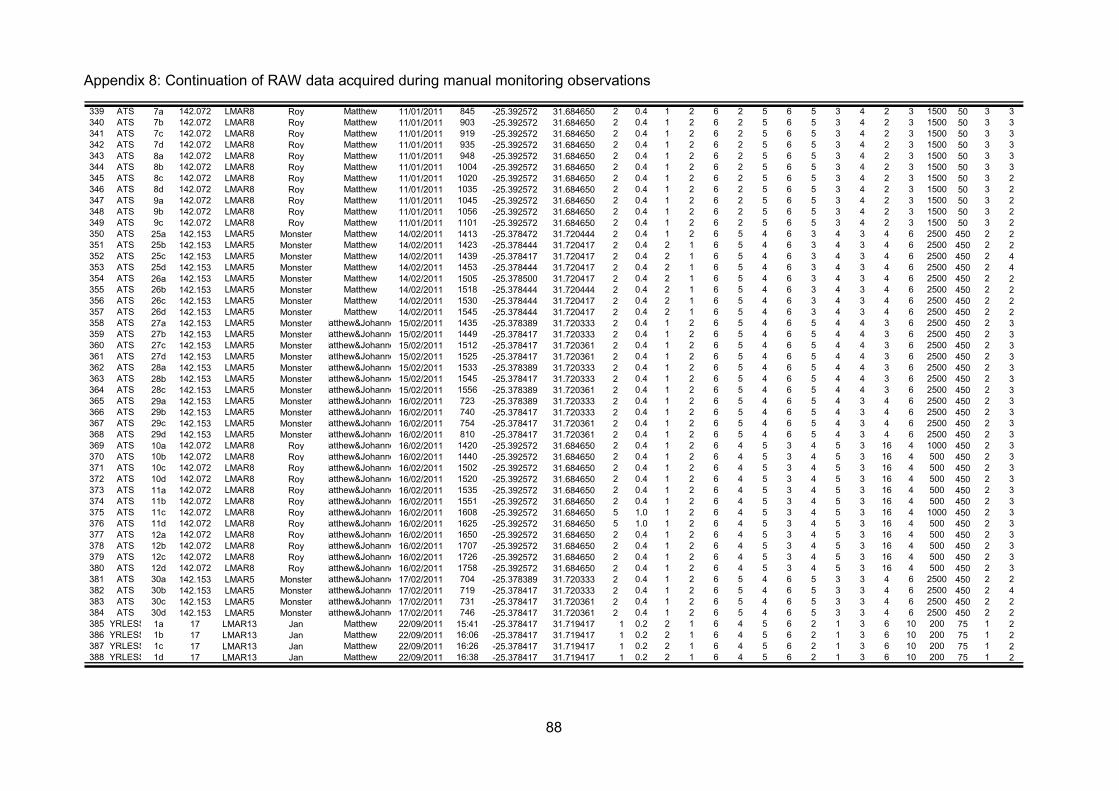
88


339 ATS 7a 142.072 LMAR8 Roy Matthew 11/01/2011 845 -25.392572 31.684650 2 0.4 1 2 6 2 5 6 5 3 4 2 3 1500 50 3 3340 ATS 7b 142.072 LMAR8 Roy Matthew 11/01/2011 903 -25.392572 31.684650 2 0.4 1 2 6 2 5 6 5 3 4 2 3 1500 50 3 3341 ATS 7c 142.072 LMAR8 Roy Matthew 11/01/2011 919 -25.392572 31.684650 2 0.4 1 2 6 2 5 6 5 3 4 2 3 1500 50 3 3342 ATS 7d 142.072 LMAR8 Roy Matthew 11/01/2011 935 -25.392572 31.684650 2 0.4 1 2 6 2 5 6 5 3 4 2 3 1500 50 3 3343 ATS 8a 142.072 LMAR8 Roy Matthew 11/01/2011 948 -25.392572 31.684650 2 0.4 1 2 6 2 5 6 5 3 4 2 3 1500 50 3 3344 ATS 8b 142.072 LMAR8 Roy Matthew 11/01/2011 1004 -25.392572 31.684650 2 0.4 1 2 6 2 5 6 5 3 4 2 3 1500 50 3 3345 ATS 8c 142.072 LMAR8 Roy Matthew 11/01/2011 1020 -25.392572 31.684650 2 0.4 1 2 6 2 5 6 5 3 4 2 3 1500 50 3 2346 ATS 8d 142.072 LMAR8 Roy Matthew 11/01/2011 1035 -25.392572 31.684650 2 0.4 1 2 6 2 5 6 5 3 4 2 3 1500 50 3 2347 ATS 9a 142.072 LMAR8 Roy Matthew 11/01/2011 1045 -25.392572 31.684650 2 0.4 1 2 6 2 5 6 5 3 4 2 3 1500 50 3 2348 ATS 9b 142.072 LMAR8 Roy Matthew 11/01/2011 1056 -25.392572 31.684650 2 0.4 1 2 6 2 5 6 5 3 4 2 3 1500 50 3 2349 ATS 9c 142.072 LMAR8 Roy Matthew 11/01/2011 1101 -25.392572 31.684650 2 0.4 1 2 6 2 5 6 5 3 4 2 3 1500 50 3 2350 ATS 25a 142.153 LMAR5 Monster Matthew 14/02/2011 1413 -25.378472 31.720444 2 0.4 1 2 6 5 4 6 3 4 3 4 6 2500 450 2 2351 ATS 25b 142.153 LMAR5 Monster Matthew 14/02/2011 1423 -25.378444 31.720417 2 0.4 2 1 6 5 4 6 3 4 3 4 6 2500 450 2 2352 ATS 25c 142.153 LMAR5 Monster Matthew 14/02/2011 1439 -25.378417 31.720417 2 0.4 2 1 6 5 4 6 3 4 3 4 6 2500 450 2 4353 ATS 25d 142.153 LMAR5 Monster Matthew 14/02/2011 1453 -25.378444 31.720417 2 0.4 2 1 6 5 4 6 3 4 3 4 6 2500 450 2 4354 ATS 26a 142.153 LMAR5 Monster Matthew 14/02/2011 1505 -25.378500 31.720417 2 0.4 2 1 6 5 4 6 3 4 3 4 6 2500 450 2 2355 ATS 26b 142.153 LMAR5 Monster Matthew 14/02/2011 1518 -25.378444 31.720444 2 0.4 2 1 6 5 4 6 3 4 3 4 6 2500 450 2 2356 ATS 26c 142.153 LMAR5 Monster Matthew 14/02/2011 1530 -25.378444 31.720417 2 0.4 2 1 6 5 4 6 3 4 3 4 6 2500 450 2 2357 ATS 26d 142.153 LMAR5 Monster Matthew 14/02/2011 1545 -25.378444 31.720417 2 0.4 2 1 6 5 4 6 3 4 3 4 6 2500 450 2 2358 ATS 27a 142.153 LMAR5 Monster Matthew&Johannes15/02/2011 1435 -25.378389 31.720333 2 0.4 1 2 6 5 4 6 5 4 4 3 6 2500 450 2 3359 ATS 27b 142.153 LMAR5 Monster Matthew&Johannes15/02/2011 1449 -25.378417 31.720333 2 0.4 1 2 6 5 4 6 5 4 4 3 6 2500 450 2 3360 ATS 27c 142.153 LMAR5 Monster Matthew&Johannes15/02/2011 1512 -25.378417 31.720361 2 0.4 1 2 6 5 4 6 5 4 4 3 6 2500 450 2 3361 ATS 27d 142.153 LMAR5 Monster Matthew&Johannes15/02/2011 1525 -25.378417 31.720361 2 0.4 1 2 6 5 4 6 5 4 4 3 6 2500 450 2 3362 ATS 28a 142.153 LMAR5 Monster Matthew&Johannes15/02/2011 1533 -25.378389 31.720333 2 0.4 1 2 6 5 4 6 5 4 4 3 6 2500 450 2 3363 ATS 28b 142.153 LMAR5 Monster Matthew&Johannes15/02/2011 1545 -25.378417 31.720333 2 0.4 1 2 6 5 4 6 5 4 4 3 6 2500 450 2 3364 ATS 28c 142.153 LMAR5 Monster Matthew&Johannes15/02/2011 1556 -25.378389 31.720361 2 0.4 1 2 6 5 4 6 5 4 4 3 6 2500 450 2 3365 ATS 29a 142.153 LMAR5 Monster Matthew&Johannes16/02/2011 723 -25.378389 31.720333 2 0.4 1 2 6 5 4 6 5 4 3 4 6 2500 450 2 3366 ATS 29b 142.153 LMAR5 Monster Matthew&Johannes16/02/2011 740 -25.378417 31.720333 2 0.4 1 2 6 5 4 6 5 4 3 4 6 2500 450 2 3367 ATS 29c 142.153 LMAR5 Monster Matthew&Johannes16/02/2011 754 -25.378417 31.720361 2 0.4 1 2 6 5 4 6 5 4 3 4 6 2500 450 2 3368 ATS 29d 142.153 LMAR5 Monster Matthew&Johannes16/02/2011 810 -25.378417 31.720361 2 0.4 1 2 6 5 4 6 5 4 3 4 6 2500 450 2 3369 ATS 10a 142.072 LMAR8 Roy Matthew&Johannes16/02/2011 1420 -25.392572 31.684650 2 0.4 1 2 6 4 5 3 4 5 3 16 4 1000 450 2 3370 ATS 10b 142.072 LMAR8 Roy Matthew&Johannes16/02/2011 1440 -25.392572 31.684650 2 0.4 1 2 6 4 5 3 4 5 3 16 4 500 450 2 3371 ATS 10c 142.072 LMAR8 Roy Matthew&Johannes16/02/2011 1502 -25.392572 31.684650 2 0.4 1 2 6 4 5 3 4 5 3 16 4 500 450 2 3372 ATS 10d 142.072 LMAR8 Roy Matthew&Johannes16/02/2011 1520 -25.392572 31.684650 2 0.4 1 2 6 4 5 3 4 5 3 16 4 500 450 2 3373 ATS 11a 142.072 LMAR8 Roy Matthew&Johannes16/02/2011 1535 -25.392572 31.684650 2 0.4 1 2 6 4 5 3 4 5 3 16 4 500 450 2 3374 ATS 11b 142.072 LMAR8 Roy Matthew&Johannes16/02/2011 1551 -25.392572 31.684650 2 0.4 1 2 6 4 5 3 4 5 3 16 4 500 450 2 3375 ATS 11c 142.072 LMAR8 Roy Matthew&Johannes16/02/2011 1608 -25.392572 31.684650 5 1.0 1 2 6 4 5 3 4 5 3 16 4 1000 450 2 3376 ATS 11d 142.072 LMAR8 Roy Matthew&Johannes16/02/2011 1625 -25.392572 31.684650 5 1.0 1 2 6 4 5 3 4 5 3 16 4 500 450 2 3377 ATS 12a 142.072 LMAR8 Roy Matthew&Johannes16/02/2011 1650 -25.392572 31.684650 2 0.4 1 2 6 4 5 3 4 5 3 16 4 500 450 2 3378 ATS 12b 142.072 LMAR8 Roy Matthew&Johannes16/02/2011 1707 -25.392572 31.684650 2 0.4 1 2 6 4 5 3 4 5 3 16 4 500 450 2 3379 ATS 12c 142.072 LMAR8 Roy Matthew&Johannes16/02/2011 1726 -25.392572 31.684650 2 0.4 1 2 6 4 5 3 4 5 3 16 4 500 450 2 3380 ATS 12d 142.072 LMAR8 Roy Matthew&Johannes16/02/2011 1758 -25.392572 31.684650 2 0.4 1 2 6 4 5 3 4 5 3 16 4 500 450 2 3381 ATS 30a 142.153 LMAR5 Monster Matthew&Johannes17/02/2011 704 -25.378389 31.720333 2 0.4 1 2 6 5 4 6 5 3 3 4 6 2500 450 2 2382 ATS 30b 142.153 LMAR5 Monster Matthew&Johannes17/02/2011 719 -25.378417 31.720333 2 0.4 1 2 6 5 4 6 5 3 3 4 6 2500 450 2 4383 ATS 30c 142.153 LMAR5 Monster Matthew&Johannes17/02/2011 731 -25.378417 31.720361 2 0.4 1 2 6 5 4 6 5 3 3 4 6 2500 450 2 2384 ATS 30d 142.153 LMAR5 Monster Matthew&Johannes17/02/2011 746 -25.378417 31.720361 2 0.4 1 2 6 5 4 6 5 3 3 4 6 2500 450 2 2385 YRLESS 1a 17 LMAR13 Jan Matthew 22/09/2011 15:41 -25.378417 31.719417 1 0.2 2 1 6 4 5 6 2 1 3 6 10 200 75 1 2386 YRLESS 1b 17 LMAR13 Jan Matthew 22/09/2011 16:06 -25.378417 31.719417 1 0.2 2 1 6 4 5 6 2 1 3 6 10 200 75 1 2387 YRLESS 1c 17 LMAR13 Jan Matthew 22/09/2011 16:26 -25.378417 31.719417 1 0.2 2 1 6 4 5 6 2 1 3 6 10 200 75 1 2388 YRLESS 1d 17 LMAR13 Jan Matthew 22/09/2011 16:38 -25.378417 31.719417 1 0.2 2 1 6 4 5 6 2 1 3 6 10 200 75 1 2

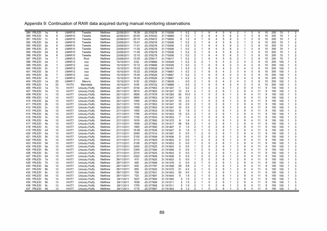
89


389 YRLESS 1a 6 LMAR10 Tweetie Matthew 22/09/2011 16:39 -25.378278 31.719306 1 0.2 2 1 6 4 5 6 2 1 3 6 10 200 75 1 2390 YRLESS 1b 6 LMAR10 Tweetie Matthew 22/09/2011 20:00 -25.378333 31.718889 1 0.2 1 2 6 4 5 6 2 1 3 6 10 200 75 1 2391 YRLESS 1c 6 LMAR10 Tweetie Matthew 22/09/2011 20:10 -25.378472 31.719000 6 1.2 4 1 6 4 5 6 2 1 3 6 10 200 75 1 2392 YRLESS 2a 6 LMAR10 Tweetie Matthew 23/09/2011 10:41 -25.378278 31.719306 1 0.2 2 1 6 4 5 6 2 1 3 6 10 200 75 1 2393 YRLESS 2b 6 LMAR10 Tweetie Matthew 23/09/2011 11:01 -25.378278 31.719306 1 0.2 2 1 6 4 5 6 2 1 3 6 10 200 75 1 2394 YRLESS 2c 6 LMAR10 Tweetie Matthew 23/09/2011 11:20 -25.378278 31.719306 1 0.2 2 1 6 4 5 6 2 1 3 6 10 200 75 1 2395 YRLESS 2d 6 LMAR10 Tweetie Matthew 23/09/2011 11:45 -25.378278 31.719306 1 0.2 2 1 6 4 5 6 2 1 3 6 10 200 75 1 2396 YRLESS 3a 6 LMAR10 Tweetie Matthew 23/09/2011 12:10 -25.378278 31.719306 1 0.2 2 1 6 4 5 6 2 1 3 6 10 200 75 1 2397 YRLESS 1a 7 LMAR12 Rooi Matthew 23/09/2011 12:25 -25.378417 31.719417 1 0.2 2 1 6 4 5 6 2 1 3 6 10 200 75 1 2398 YRLESS 2a 7 LMAR12 rooi Matthew 15/10/2011 9:52 -25.378666 31.723029 1 0.2 5 2 1 5 4 2 3 4 3 6 10 200 100 1 3399 YRLESS 2b 7 LMAR12 rooi Matthew 15/10/2011 10:12 -25.378666 31.723029 1 0.2 2 1 6 5 4 2 3 4 3 6 10 200 100 1 3400 YRLESS 2c 7 LMAR12 rooi Matthew 15/10/2011 10:22 -25.378528 31.744167 1 0.2 2 1 6 5 4 2 3 4 3 6 10 200 100 1 3401 YRLESS 3a 7 LMAR12 rooi Matthew 15/10/2011 15:22 -25.378528 31.719667 1 0.2 2 1 6 5 4 2 3 4 3 6 10 200 100 1 3402 YRLESS 3b 7 LMAR12 rooi Matthew 15/10/2011 15:40 -25.378528 31.719667 1 0.2 2 1 6 5 4 2 3 4 3 6 10 200 100 1 3403 YRLESS 3c 7 LMAR12 rooi Matthew 15/10/2011 16:30 -25.378528 31.719667 1 0.2 2 1 6 5 4 2 3 4 3 6 10 200 100 1 3404 YRLESS 1a 25 LMAR11 Mary-lu Matthew 15/10/2011 9:30 -25.378361 31.718639 - 0.0 2 1 6 5 4 2 4 3 3 6 10 200 100 1 3405 YRLESS 1a 23 HVIT4 Mannetjie Matthew 15/10/2011 9:48 -25.378722 31.718889 - 0.0 2 1 6 5 4 2 4 3 3 6 10 200 100 1 3406 YRLESS 1a 13 HVIT7 Unlucky Fluffy Matthew 25/11/2011 0730 -25.377853 31.741347 1 0.2 2 1 0 2 6 1 2 9 4 11 9 150 100 1 3407 YRLESS 1b 13 HVIT7 Unlucky Fluffy Matthew 25/11/2011 0810 -25.377853 31.741347 10 2.0 2 1 0 2 6 1 2 9 4 11 9 150 100 1 3408 YRLESS 1c 13 HVIT7 Unlucky Fluffy Matthew 25/11/2011 0826 -25.377978 31.741283 50 10.0 2 1 0 2 6 1 2 9 4 11 9 150 100 1 3409 YRLESS 1d 13 HVIT7 Unlucky Fluffy Matthew 25/11/2011 0850 -25.377853 31.741347 10 2.0 2 1 0 2 6 1 2 9 4 11 9 150 100 1 3410 YRLESS 2a 13 HVIT7 Unlucky Fluffy Matthew 25/11/2011 1000 -25.377853 31.741347 10 2.0 2 1 0 2 6 1 2 9 4 11 9 150 100 1 3411 YRLESS 2b 13 HVIT7 Unlucky Fluffy Matthew 25/11/2011 1016 -25.377853 31.741347 10 2.0 2 1 0 2 6 1 2 9 4 11 9 150 100 1 3412 YRLESS 2c 13 HVIT7 Unlucky Fluffy Matthew 25/11/2011 1056 -25.377853 31.741347 10 2.0 2 1 0 2 6 1 2 9 4 11 9 150 100 1 3413 YRLESS 3a 13 HVIT7 Unlucky Fluffy Matthew 27/11/2011 1455 -25.377633 31.741503 9 1.8 2 1 0 2 6 1 2 9 4 11 9 150 100 1 3414 YRLESS 3b 13 HVIT7 Unlucky Fluffy Matthew 27/11/2011 1706 -25.377633 31.741503 10 2.0 2 1 0 2 6 1 2 9 4 11 9 150 100 1 3415 YRLESS 3c 13 HVIT7 Unlucky Fluffy Matthew 27/11/2011 1725 -25.377633 31.741503 7 1.4 2 1 0 2 6 1 2 9 4 11 9 150 100 1 3416 YRLESS 4a 13 HVIT7 Unlucky Fluffy Matthew 27/11/2011 1816 -25.377850 31.741375 8 1.6 2 1 0 2 6 1 2 9 4 11 9 150 100 1 3417 YRLESS 4b 13 HVIT7 Unlucky Fluffy Matthew 27/11/2011 1839 -25.377883 31.741417 48 9.6 2 1 0 2 6 1 2 9 4 11 9 150 100 1 3418 YRLESS 4c 13 HVIT7 Unlucky Fluffy Matthew 27/11/2011 1900 -25.377950 31.741467 5 1.0 2 1 0 2 6 1 2 9 4 11 9 150 100 1 3419 YRLESS 4d 13 HVIT7 Unlucky Fluffy Matthew 27/11/2011 19:26 -25.377639 31.741647 8 1.6 2 1 0 2 6 1 2 9 4 11 9 150 100 1 3420 YRLESS 5a 13 HVIT7 Unlucky Fluffy Matthew 27/11/2011 2046 -25.377510 31.741597 0 0.0 1 2 0 2 6 1 2 9 4 11 9 150 100 1 3421 YRLESS 5b 13 HVIT7 Unlucky Fluffy Matthew 27/11/2011 2100 -25.377608 31.741606 0 0.0 1 2 0 2 6 1 2 9 4 11 9 150 100 1 3422 YRLESS 5c 13 HVIT7 Unlucky Fluffy Matthew 27/11/2011 2113 -25.377625 31.741603 0 0.0 1 2 0 2 6 1 2 9 4 11 9 150 100 1 3423 YRLESS 5d 13 HVIT7 Unlucky Fluffy Matthew 27/11/2011 2126 -25.377625 31.741603 0 0.0 1 2 0 2 6 1 2 9 4 11 9 150 100 1 3424 YRLESS 6a 13 HVIT7 Unlucky Fluffy Matthew 27/11/2011 2240 -25.377625 31.741603 0 0.0 1 2 0 2 6 1 2 9 4 11 9 150 100 1 3425 YRLESS 6b 13 HVIT7 Unlucky Fluffy Matthew 27/11/2011 2305 -25.377594 31.741606 0 0.0 1 2 0 2 6 1 2 9 4 11 9 150 100 1 3426 YRLESS 6c 13 HVIT7 Unlucky Fluffy Matthew 27/11/2011 2314 -25.377625 31.741603 0 0.0 1 2 0 2 6 1 2 9 4 11 9 150 100 1 3427 YRLESS 6d 13 HVIT7 Unlucky Fluffy Matthew 27/11/2011 2322 -25.377608 31.741608 0 0.0 1 2 0 2 6 1 2 9 4 11 9 150 100 1 3428 YRLESS 7a 13 HVIT7 Unlucky Fluffy Matthew 28/11/2011 410 -25.377625 31.741603 0 0.0 1 2 0 2 6 1 2 9 4 11 9 150 100 1 3429 YRLESS 7b 13 HVIT7 Unlucky Fluffy Matthew 28/11/2011 426 -25.377656 31.741378 0 0.0 2 1 0 2 6 1 2 9 4 11 9 150 100 1 3430 YRLESS 8a 13 HVIT7 Unlucky Fluffy Matthew 28/11/2011 635 -25.377797 31.741508 29 5.8 2 1 0 2 6 1 2 9 4 11 9 150 100 1 3431 YRLESS 8b 13 HVIT7 Unlucky Fluffy Matthew 28/11/2011 655 -25.377825 31.741575 21 4.2 2 1 0 2 6 1 2 9 4 11 9 150 100 1 3432 YRLESS 8c 13 HVIT7 Unlucky Fluffy Matthew 28/11/2011 709 -25.377931 31.741453 25 5.0 2 1 0 2 6 1 2 9 4 11 9 150 100 1 3433 YRLESS 8d 13 HVIT7 Unlucky Fluffy Matthew 28/11/2011 725 -25.377997 31.741644 9 1.8 2 1 0 2 6 1 2 9 4 11 9 150 100 1 3434 YRLESS 9a 13 HVIT7 Unlucky Fluffy Matthew 29/112011 1637 -25.377900 31.741483 5 1.0 2 1 0 2 6 1 2 9 4 11 9 150 100 1 3435 YRLESS 9b 13 HVIT7 Unlucky Fluffy Matthew 29/112011 1638 -25.377908 31.741511 5 1.0 2 1 0 2 6 1 2 9 4 11 9 150 100 1 3436 YRLESS 9c 13 HVIT7 Unlucky Fluffy Matthew 29/112011 1705 -25.377908 31.741511 5 1.0 2 1 0 2 6 1 2 9 4 11 9 150 100 1 3437 YRLESS 9d 13 HVIT7 Unlucky Fluffy Matthew 29/112011 1715 -25.377867 31.741403 6 1.2 2 1 0 2 6 1 2 9 4 11 9 150 100 1 3

90


438 YRLESS 10a 13 HVIT7 Unlucky Fluffy Matthew 29/112011 1800 -25.377908 31.741511 40 8.0 2 1 0 2 6 1 2 9 4 11 9 150 100 1 3439 YRLESS 10b 13 HVIT7 Unlucky Fluffy Matthew 29/112011 1801 -25.377867 31.741403 1 0.2 2 1 0 2 6 1 2 9 4 11 9 150 100 1 3440 YRLESS 10c 13 HVIT7 Unlucky Fluffy Matthew 29/112011 1821 -25.377772 31.741272 9 1.8 2 1 0 2 6 1 2 9 4 11 9 150 100 1 3441 YRLESS 10d 13 HVIT7 Unlucky Fluffy Matthew 29/112011 1831 -25.377908 31.741583 24 4.8 2 1 0 2 6 1 2 9 4 11 9 150 100 1 3442 YRLESS 11a 13 HVIT7 Unlucky Fluffy Matthew 29/112011 18:42 -25.377833 31.741264 55 11.0 2 1 0 2 6 1 2 9 4 11 9 150 100 1 3443 YRLESS 11b 13 HVIT7 Unlucky Fluffy Matthew 29/112011 1855 -25.377675 31.741586 19 3.8 2 1 0 2 6 1 2 9 4 11 9 150 100 1 3444 YRLESS 12a 13 HVIT7 Unlucky Fluffy Matthew 29/112011 2035 -25.377681 31.741050 1 0.2 1 2 0 2 6 1 2 9 4 11 9 150 100 1 3445 YRLESS 12b 13 HVIT7 Unlucky Fluffy Matthew 29/112011 2102 -25.377719 31.741064 1 0.2 1 2 0 2 6 1 2 9 4 11 9 150 100 1 3446 YRLESS 13a 13 HVIT7 Unlucky Fluffy Matthew 30/11/2011 415 -25.377650 31.741667 4 0.8 1 2 0 2 6 1 2 9 4 11 9 150 100 1 3447 YRLESS 13b 13 HVIT7 Unlucky Fluffy Matthew 30/11/2011 432 -25.377619 31.741572 80 16.0 2 1 0 2 6 1 2 9 4 11 9 150 100 1 3448 YRLESS 13c 13 HVIT7 Unlucky Fluffy Matthew 30/11/2011 446 -25.377975 31.741572 22 4.4 2 1 0 2 6 1 2 9 4 11 9 150 100 1 3449 YRLESS 13d 13 HVIT7 Unlucky Fluffy Matthew 30/11/2011 502 -25.377975 31.741597 40 8.0 2 1 0 2 6 1 2 9 4 11 9 150 100 1 3450 YRLESS 14a 13 HVIT7 Unlucky Fluffy Matthew 30/11/2011 543 -25.377975 31.741597 24 4.8 2 1 0 2 6 1 2 9 4 11 9 150 100 1 3451 YRLESS 14b 13 HVIT7 Unlucky Fluffy Matthew 30/11/2011 600 -25.377975 31.741597 34 6.8 2 1 0 2 6 1 2 9 4 11 9 150 100 1 3452 YRLESS 14c 13 HVIT7 Unlucky Fluffy Matthew 30/11/2011 610 -25.377975 31.741597 26 5.2 2 1 0 2 6 1 2 9 4 11 9 150 100 1 3453 YRLESS 14d 13 HVIT7 Unlucky Fluffy Matthew 30/11/2011 620 -25.377975 31.741597 36 7.2 2 1 0 2 6 1 2 9 4 11 9 150 100 1 3454 YRLESS 15a 13 HVIT7 Unlucky Fluffy Matthew 30/11/2011 720 -25.377975 31.741597 81 16.2 2 1 0 2 6 1 2 9 4 11 9 150 100 1 3455 YRLESS 16a 13 HVIT7 Unlucky Fluffy Matthew 1/12/2011 1710 -25.377894 31.741483 9 1.8 2 1 0 2 6 1 2 9 4 11 9 150 100 1 3456 YRLESS 16b 13 HVIT7 Unlucky Fluffy Matthew 1/12/2011 1730 -25.377811 31.741481 50 10.0 2 1 0 2 6 1 2 9 4 11 9 150 100 1 3457 YRLESS 16c 13 HVIT7 Unlucky Fluffy Matthew 1/12/2011 1745 -25.377822 31.741569 70 14.0 2 1 0 2 6 1 2 9 4 11 9 150 100 1 3458 YRLESS 16d 13 HVIT7 Unlucky Fluffy Matthew 1/12/2011 1758 -25.377717 31.741161 9 1.8 2 1 0 2 6 1 2 9 4 11 9 150 100 1 3459 YRLESS 17a 13 HVIT7 Unlucky Fluffy Matthew 1/12/2011 1822 -25.377772 31.741322 26 5.2 2 1 0 2 6 1 2 9 4 11 9 150 100 1 3460 YRLESS 17b 13 HVIT7 Unlucky Fluffy Matthew 1/12/2011 1831 -25.377750 31.741236 34 6.8 2 1 0 2 6 1 2 9 4 11 9 150 100 1 3461 YRLESS 17c 13 HVIT7 Unlucky Fluffy Matthew 27/11/2011 1845 -25.377875 31.741267 42 8.4 2 1 0 2 6 1 2 9 4 11 9 150 100 1 1462 YRLESS 17d 13 HVIT7 Unlucky Fluffy Matthew 27/11/2011 1900 -25.377767 31.741272 24 4.8 2 1 0 2 6 1 2 9 4 11 9 150 100 1 3463 YRLESS 18a 13 HVIT7 Unlucky Fluffy Matthew 27/11/2011 2008 -25.377739 31.741247 4 0.8 2 1 0 2 6 1 2 9 4 11 9 150 100 1 3464 YRLESS 18b 13 HVIT7 Unlucky Fluffy Matthew 28/11/2011 2104 -25.377664 31.741681 1 0.2 1 2 0 2 6 1 2 9 4 11 9 150 100 1 3465 YRLESS 18c 13 HVIT7 Unlucky Fluffy Matthew 28/11/2011 2114 -25.377664 31.741681 1 0.2 1 2 0 2 6 1 2 9 4 11 9 150 100 1 3466 YRLESS 18d 13 HVIT7 Unlucky Fluffy Matthew 28/11/2011 2130 -25.377664 31.741681 0 0.0 1 2 0 2 6 1 2 9 4 11 9 150 100 1 3467 YRLESS 19a 13 HVIT7 Unlucky Fluffy Matthew 28/11/2011 415 -25.377664 31.741681 0 0.0 1 2 0 2 6 1 2 9 4 11 9 150 100 1 3468 YRLESS 19b 13 HVIT7 Unlucky Fluffy Matthew 28/11/2011 430 -25.377664 31.741681 5 1.0 1 2 0 2 6 1 2 9 4 11 9 150 100 1 3469 YRLESS 19c 13 HVIT7 Unlucky Fluffy Matthew 28/11/2011 445 -25.377692 31.741606 0 0.0 1 2 0 2 6 1 2 9 4 11 9 150 100 1 3470 YRLESS 19d 13 HVIT7 Unlucky Fluffy Matthew 28/11/2011 430 -25.377692 31.741606 57 11.4 2 1 0 2 6 1 2 9 4 11 9 150 100 1 3471 YRLESS 20a 13 HVIT7 Unlucky Fluffy Matthew 28/11/2011 448 -25.377692 31.741606 55 11.0 2 1 0 2 6 1 2 9 4 11 9 150 100 1 3472 YRLESS 20b 13 HVIT7 Unlucky Fluffy Matthew 28/11/2011 500 -25.377692 31.741606 53 10.6 2 1 0 2 6 1 2 9 4 11 9 150 100 1 3473 YRLESS 20c 13 HVIT7 Unlucky Fluffy Matthew 28/11/2011 507 -25.377692 31.741606 56 11.2 2 1 0 2 6 1 2 9 4 11 9 150 100 1 3474 YRLESS 20d 13 HVIT7 Unlucky Fluffy Matthew 28/11/2011 517 -25.377783 31.741686 27 5.4 2 1 0 2 6 1 2 9 4 11 9 150 100 1 3475 YRLESS 21a 13 HVIT7 Unlucky Fluffy Matthew 28/11/2011 600 -25.377861 31.741553 51 10.2 2 1 0 2 6 1 2 9 4 11 9 150 100 1 4476 YRLESS 21b 13 HVIT7 Unlucky Fluffy Matthew 28/11/2011 615 -25.377861 31.741556 9 1.8 2 1 0 2 6 1 2 9 4 11 9 150 100 1 4477 YRLESS 21c 13 HVIT7 Unlucky Fluffy Matthew 28/11/2011 628 -25.377822 31.741519 24 4.8 2 1 0 2 6 1 2 9 4 11 9 150 100 1 4478 YRLESS 21d 13 HVIT7 Unlucky Fluffy Matthew 28/11/2011 640 -25.377900 31.741564 20 4.0 2 1 0 2 6 1 2 9 4 11 9 150 100 1 4479 YRLESS 22a 13 HVIT7 Unlucky Fluffy Matthew 28/11/2011 745 -25.377950 31.741633 60 12.0 2 1 0 2 6 1 2 9 4 11 9 150 100 1 4

91

Appendix 11: Graphical representation of the home for the 2.5 kg Labeobarbus marequensis

LMAR1, with ATS tag 2030 frequency 142.214. Tagged on the 15/08/2009 and monitored

until the 19/09/2009, monitored on 15 occasions.

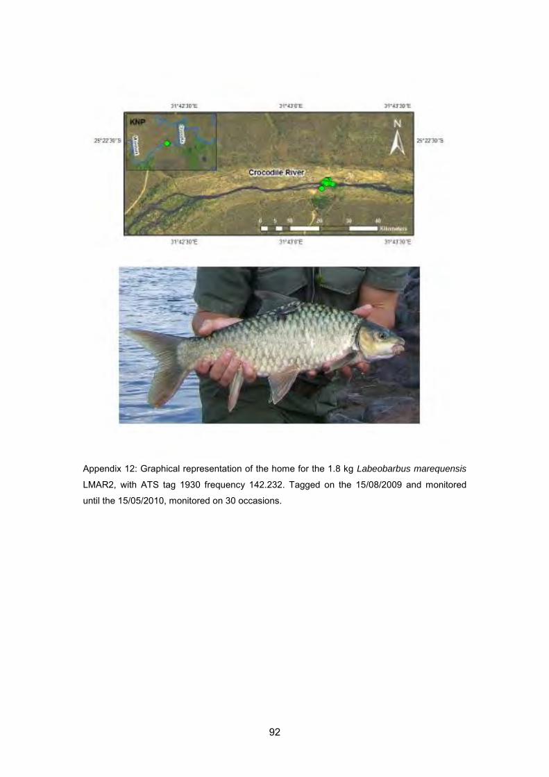
92




93




94




95




96




97

Appendix 17: Graphical representation of the home for the 3 kg Labeobarbus marequensis



98




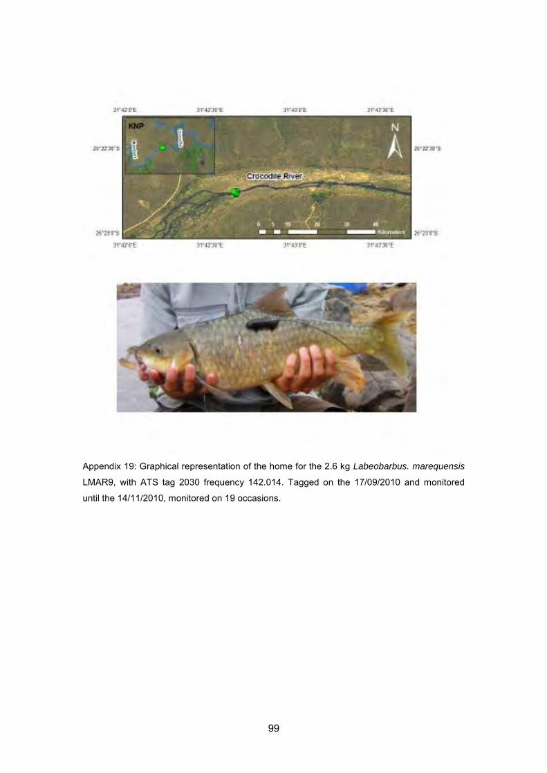
99

Appendix 19: Graphical representation of the home for the 2.6 kg Labeobarbus. marequensis



100

Appendix 20: Graphical depiction of: The 2.5 kg Labeobarbus marequensis LMAR10, with WW tag Series IV no. 6, tagged on the 19/09/2011, tag active until

the 01/06/2012 (A). The 2.8 kg L. marequensis LMAR11, with WW tag Series III no. 25, tagged on the 19/09/2011, tag active until the 01/06/2012 (B). The 2.5

kg L. marequensis LMAR12, with WW tag Series IV no. 7, tagged on the 19/09/2011, tag active until the 01/06/2012 (C). The 2.3 kg L. marequensis LMAR13,

with WW tag Series III no. 17, tagged on the 19/09/2011, tag active until the 01/06/2012 (D). The 2.2 kg L. marequensis LMAR14, with WW tag Series III no.

12, tagged on the 19/09/2011, tag active until the 01/06/2012 (E). The 2.3 kg L. marequensis LMAR15, with WW tag Series III no. 14, tagged on the

15/10/2011, tag active until the 01/06/2012 (F). The 3.9 kg L. marequensis LMAR16, with WW tag Series V no. 42, tagged on the 29/11//2011, active until the

01/06/2012 (G).

A B

F

C

D E

101

Appendix 21: Graphical depiction of: The 1.3 kg Hydrocynus vittatus HVIT1, with ATS tag 2060b frequency 142.322, tagged on the 19/08/2009 and Found in a

fish eagles nest on the 19/09/2009 (A). The 500 g H. vittatus HVIT2, with ATS tag 1930 frequency 142.132, tagged on the 19/08/2009 and never found again

(B). The 2.2 kg H. vittatus HVIT3, with WW tag Series III no. 21, tagged on the 16/09//2011, tag active until the 01/06/2012 (C). The 1.3 kg H. vittatus HVIT4,

with WW tag Series III no. 23, tagged on the 19/09//2011, tag active until the 01/06/2012 (D). The 2.5 kg H. vittatus HVIT5, with WW tag Series III no. 19,

tagged on the 19/09//2011, tag active until the 01/06/2012 (E). The 1.7 kg H. vittatus HVIT6, with WW tag Series III no. 9, tagged on the 19/09//2011, tag active

until the 01/06/2012 (F). The 2.1 kg H. vittatus HVIT7, with WW tag Series III no. 13, tagged on the 22/09//2011, tag active until the 01/06/2012 (G). The 4 kg H.

vittatus HVIT8, with WW tag Series III no. 15, tagged on the 22/10//2011, tag active until the 01/06/2012 (J). The 2 kg H. vittatus HVIT9, with WW tag Series III

no. 16, tagged on the 04/11//2011, tag active until the 01/06/2012 (H). The 3 kg H. vittatus HVIT10, with WW tag Series V no. 41, tagged on the 23/11//2011,

tag active until the 01/06/2012 (I). The 2.1 kg H. vittatus HVIT11, with WW tag Series III no. 31, tagged on the 26/11//2011, tag active until the 01/06/2012 (K).

The 2.1 kg H. vittatus HVIT12, with WW tag Series III no. 35 tagged on the 28/11//2011, tag active until the 01/06/2012 (L).

A C DB

E

F G H

I

JK

L

adult owveld largescale yellowfish abeobarbusmjejane game reserve, especially j. bardenhorst who...

Documents