advanced analytics methodologies -...
TRANSCRIPT

Advanced Analytics Methodologies
Driving Business Value with Analytics
Michele Chambers Thomas W. Dinsmore

Associate Publisher and Director of Marketing: Amy Neidlinger Executive Editor: Jeanne Glasser Levine Operations Specialist: Jodi Kemper Cover Designer: Alan Clements Managing Editor: Kristy Hart Project Editors: Melissa Schirmer, Elaine Wiley Copy Editor: Chuck Hutchinson Proofreader: Jess DeGabriele Senior Indexer: Cheryl Lenser Compositor: Nonie Ratcliff Manufacturing Buyer: Dan Uhrig
© 2015 by Pearson Education, Inc.
Upper Saddle River, New Jersey 07458
For information about buying this title in bulk quantities, or for special sales opportunities (which may include electronic versions; custom cover designs; and content particular to your business, training goals, marketing focus, or branding interests), please contact our corporate sales department at [email protected] or (800) 382-3419.
For government sales inquiries, please contact [email protected] .
For questions about sales outside the U.S., please contact [email protected] .
Company and product names mentioned herein are the trademarks or registered trademarks of their respective owners.
All rights reserved. No part of this book may be reproduced, in any form or by any means, without permission in writing from the publisher.
Printed in the United States of America
First Printing September 2014
ISBN-10: 0-13-349860-3 ISBN-13: 978-0-13-349860-8
Pearson Education LTD. Pearson Education Australia PTY, Limited. Pearson Education Singapore, Pte. Ltd. Pearson Education Asia, Ltd. Pearson Education Canada, Ltd. Pearson Educación de Mexico, S.A. de C.V. Pearson Education—Japan Pearson Education Malaysia, Pte. Ltd.
Library of Congress Control Number: 2014943265

To my son, Cole, may you help make the world a better place with your math, science, and technology
talent. To my mother, who taught me how to be graceful and loving. To my father, who passed his
math gene on to me and taught me that there are no limits in life other than those you impose on yourself. To my adopted family, Lisa, Pei Yee, Patrick, Jenny,
and Angel, thank you for your love and support.
To the heroes on the front line and those behind the scenes who are working toward
eradicating slavery from the face of the earth—may analytic insights help in some small way
to achieve this quest in your lifetime. —Michele
To my wife, Ann; my two sons, Thomas and Michael;
my late nephew Jeffrey Thomas Dinsmore; my father, Ralph Boone Dinsmore;
and to my grandfather E.W. Egee Jr., who loved new technology.
—Thomas

This page intentionally left blank
Contents
Chapter 1 Principles of Modern Analytics . . . . . . . . . . . . . . . . . . . . . . 1
Deliver Business Value and Impact . . . . . . . . . . . . . . . . . . . . 3Focus on the Last Mile . . . . . . . . . . . . . . . . . . . . . . . . . . . . . . 4Leverage Kaizen . . . . . . . . . . . . . . . . . . . . . . . . . . . . . . . . . . . 6Accelerate Learning and Execution. . . . . . . . . . . . . . . . . . . . 7Differentiate Your Analytics. . . . . . . . . . . . . . . . . . . . . . . . . . 8Embed Analytics . . . . . . . . . . . . . . . . . . . . . . . . . . . . . . . . . . . 9Establish Modern Analytics Architecture . . . . . . . . . . . . . . . 9Build on Human Factors . . . . . . . . . . . . . . . . . . . . . . . . . . . 11Capitalize on Consumerization . . . . . . . . . . . . . . . . . . . . . . 12Summary . . . . . . . . . . . . . . . . . . . . . . . . . . . . . . . . . . . . . . . . 13
Chapter 2 Business 3.0 Is Here . . . . . . . . . . . . . . . . . . . . . . . . . . . . . 15
Chapter 3 Why You Need a Unique Analytics Roadmap . . . . . . . . . 19
Overview . . . . . . . . . . . . . . . . . . . . . . . . . . . . . . . . . . . . . . . . 19Business Area . . . . . . . . . . . . . . . . . . . . . . . . . . . . . . . . . . . . 20Data . . . . . . . . . . . . . . . . . . . . . . . . . . . . . . . . . . . . . . . . . . . . 21Approach . . . . . . . . . . . . . . . . . . . . . . . . . . . . . . . . . . . . . . . . 21Precision . . . . . . . . . . . . . . . . . . . . . . . . . . . . . . . . . . . . . . . . 22Algorithms . . . . . . . . . . . . . . . . . . . . . . . . . . . . . . . . . . . . . . . 23Embedding . . . . . . . . . . . . . . . . . . . . . . . . . . . . . . . . . . . . . . 23Speed. . . . . . . . . . . . . . . . . . . . . . . . . . . . . . . . . . . . . . . . . . . 23Summary . . . . . . . . . . . . . . . . . . . . . . . . . . . . . . . . . . . . . . . . 24
Chapter 4 Analytics Can Supercharge Your Business Strategy. . . . . 25
Overview . . . . . . . . . . . . . . . . . . . . . . . . . . . . . . . . . . . . . . . . 25Case Studies . . . . . . . . . . . . . . . . . . . . . . . . . . . . . . . . . . . . . 26Summary . . . . . . . . . . . . . . . . . . . . . . . . . . . . . . . . . . . . . . . . 51
Chapter 5 Building Your Analytics Roadmap . . . . . . . . . . . . . . . . . . 61
Overview . . . . . . . . . . . . . . . . . . . . . . . . . . . . . . . . . . . . . . . . 61Step 1: Identify Key Business Objectives . . . . . . . . . . . . . . 61Step 2: Define Your Value Chain. . . . . . . . . . . . . . . . . . . . . 62Step 3: Brainstorm Analytic Solution Opportunities. . . . . . 64Step 4: Describe Analytic Solution Opportunities . . . . . . . 70
vi ADVANCED ANALYTICS METHODOLOGIES
Step 5: Create Decision Model . . . . . . . . . . . . . . . . . . . . . . 74Step 6: Evaluate Analytic Solution Opportunities . . . . . . . . 75Step 7: Establish Analytics Roadmap. . . . . . . . . . . . . . . . . . 83Step 8: Evolve Your Analytics Roadmap . . . . . . . . . . . . . . . 86Summary . . . . . . . . . . . . . . . . . . . . . . . . . . . . . . . . . . . . . . . . 86
Chapter 6 Analytic Applications . . . . . . . . . . . . . . . . . . . . . . . . . . . . . 87
Overview . . . . . . . . . . . . . . . . . . . . . . . . . . . . . . . . . . . . . . . . 87Strategic Analytics. . . . . . . . . . . . . . . . . . . . . . . . . . . . . . . . . 88Managerial Analytics. . . . . . . . . . . . . . . . . . . . . . . . . . . . . . . 93Operational Analytics . . . . . . . . . . . . . . . . . . . . . . . . . . . . . . 95Scientific Analytics . . . . . . . . . . . . . . . . . . . . . . . . . . . . . . . . 98Customer-Facing Analytics . . . . . . . . . . . . . . . . . . . . . . . . . 99Summary . . . . . . . . . . . . . . . . . . . . . . . . . . . . . . . . . . . . . . . 102
Chapter 7 Analytic Use Cases . . . . . . . . . . . . . . . . . . . . . . . . . . . . . . 103
Overview . . . . . . . . . . . . . . . . . . . . . . . . . . . . . . . . . . . . . . . 103Prediction . . . . . . . . . . . . . . . . . . . . . . . . . . . . . . . . . . . . . . 106Explanation . . . . . . . . . . . . . . . . . . . . . . . . . . . . . . . . . . . . . 109Forecasting . . . . . . . . . . . . . . . . . . . . . . . . . . . . . . . . . . . . . 110Discovery. . . . . . . . . . . . . . . . . . . . . . . . . . . . . . . . . . . . . . . 111Simulation . . . . . . . . . . . . . . . . . . . . . . . . . . . . . . . . . . . . . . 116Optimization . . . . . . . . . . . . . . . . . . . . . . . . . . . . . . . . . . . . 117Summary . . . . . . . . . . . . . . . . . . . . . . . . . . . . . . . . . . . . . . . 117
Chapter 8 Predictive Analytics Methodology. . . . . . . . . . . . . . . . . . 119
Overview: The Modern Analytics Approach . . . . . . . . . . . 119Define Business Needs. . . . . . . . . . . . . . . . . . . . . . . . . . . . 122Build the Analysis Data Set . . . . . . . . . . . . . . . . . . . . . . . . 128Build the Predictive Model . . . . . . . . . . . . . . . . . . . . . . . . 133Deploy the Predictive Model . . . . . . . . . . . . . . . . . . . . . . . 141Summary . . . . . . . . . . . . . . . . . . . . . . . . . . . . . . . . . . . . . . . 146
Chapter 9 Predictive Analytics Techniques . . . . . . . . . . . . . . . . . . . 147
Overview . . . . . . . . . . . . . . . . . . . . . . . . . . . . . . . . . . . . . . . 147Statistics and Machine Learning . . . . . . . . . . . . . . . . . . . . 149The Impact of Big Data . . . . . . . . . . . . . . . . . . . . . . . . . . . 150Supervised and Unsupervised Learning . . . . . . . . . . . . . . 152Linear Models and Linear Regression. . . . . . . . . . . . . . . . 161Generalized Linear Models . . . . . . . . . . . . . . . . . . . . . . . . 167
CONTENTS vii
Generalized Additive Models. . . . . . . . . . . . . . . . . . . . . . . 168Logistic Regression . . . . . . . . . . . . . . . . . . . . . . . . . . . . . . . 169Enhanced Regression . . . . . . . . . . . . . . . . . . . . . . . . . . . . . 170Survival Analysis . . . . . . . . . . . . . . . . . . . . . . . . . . . . . . . . . 173Decision Tree Learning . . . . . . . . . . . . . . . . . . . . . . . . . . . 174Bayesian Methods . . . . . . . . . . . . . . . . . . . . . . . . . . . . . . . . 177Neural Networks and Deep Learning . . . . . . . . . . . . . . . . 178Support Vector Machines. . . . . . . . . . . . . . . . . . . . . . . . . . 183Ensemble Learning . . . . . . . . . . . . . . . . . . . . . . . . . . . . . . 184Automated Learning. . . . . . . . . . . . . . . . . . . . . . . . . . . . . . 187Summary . . . . . . . . . . . . . . . . . . . . . . . . . . . . . . . . . . . . . . . 191
Chapter 10 End User Analytics . . . . . . . . . . . . . . . . . . . . . . . . . . . . . 193
Overview . . . . . . . . . . . . . . . . . . . . . . . . . . . . . . . . . . . . . . . 193User Personas . . . . . . . . . . . . . . . . . . . . . . . . . . . . . . . . . . . 195Analytic Programming Languages . . . . . . . . . . . . . . . . . . . 199Business User Tools . . . . . . . . . . . . . . . . . . . . . . . . . . . . . . 209Summary . . . . . . . . . . . . . . . . . . . . . . . . . . . . . . . . . . . . . . . 220
Chapter 11 Analytic Platforms . . . . . . . . . . . . . . . . . . . . . . . . . . . . . . 223
Overview . . . . . . . . . . . . . . . . . . . . . . . . . . . . . . . . . . . . . . . 223Distributed Analytics . . . . . . . . . . . . . . . . . . . . . . . . . . . . . 224Predictive Analytics Architecture. . . . . . . . . . . . . . . . . . . . 228Modern SQL Platforms . . . . . . . . . . . . . . . . . . . . . . . . . . . 243Summary . . . . . . . . . . . . . . . . . . . . . . . . . . . . . . . . . . . . . . . 256
Chapter 12 Attracting and Retaining Analytics Talent . . . . . . . . . . . 257
Overview . . . . . . . . . . . . . . . . . . . . . . . . . . . . . . . . . . . . . . . 257Culture . . . . . . . . . . . . . . . . . . . . . . . . . . . . . . . . . . . . . . . . 258Data Scientist Role . . . . . . . . . . . . . . . . . . . . . . . . . . . . . . . 262Summary . . . . . . . . . . . . . . . . . . . . . . . . . . . . . . . . . . . . . . . 281
Chapter 13 Organizing Analytics Teams . . . . . . . . . . . . . . . . . . . . . . 283
Overview . . . . . . . . . . . . . . . . . . . . . . . . . . . . . . . . . . . . . . . 283Centralized versus Decentralized Analytics Team . . . . . . 283Center of Excellence . . . . . . . . . . . . . . . . . . . . . . . . . . . . . 288Chief Data Officer versus Chief Analytics Officer . . . . . . 289Lab Team . . . . . . . . . . . . . . . . . . . . . . . . . . . . . . . . . . . . . . 291Analytic Program Office . . . . . . . . . . . . . . . . . . . . . . . . . . . 291Summary . . . . . . . . . . . . . . . . . . . . . . . . . . . . . . . . . . . . . . . 291

viii ADVANCED ANALYTICS METHODOLOGIES
Chapter 14 What Are You Waiting For? Go Get Started!. . . . . . . . . 293
Appendix A Unsupervised Learning: Unsupervised Neural Networks . . . . . . . . . . . . . . . . . . . . . . . . . . . . . . . . . . . . . 297
Unsupervised Feed-Forward Architectures . . . . . . . . . . . 298Kohonen’s Self-Organizing Map . . . . . . . . . . . . . . . . . . . . 299Related Neural Network Architectures . . . . . . . . . . . . . . . 304Examples and Related Neural Network Models . . . . . . . . 307References. . . . . . . . . . . . . . . . . . . . . . . . . . . . . . . . . . . . . . 310
Index. . . . . . . . . . . . . . . . . . . . . . . . . . . . . . . . . . . . . . . . . 313

Foreword
In the era of Big Data, customers increasingly recognize the value that advanced analytics offers to differentiate their business. As a result, predictive models turn into critical business assets that can deliver huge benefits, but also require a more rigorous process for the operational deployment in order to generate such business value.
In this context, it is shocking to see that only a small percentage of predictive models are actually deployed and that deployment often takes several months. Organizations face a wide range of business requirements, a host of operational IT solutions and data warehouse platforms, plus a rapidly growing set of data mining tools. For an orga-nization to truly take advantage of the opportunities that advanced analytics has to offer, it needs to break old habits, often constrained by single-vendor solutions or manual processes, and move toward a modern analytics infrastructure. It is no surprise that in a recent set of reports, Gartner emphasized the benefits that vendor-neutral indus-try standards and open software platforms offer to end user organi-zations in many industries to rapidly deploy and execute predictive models across a wide range of hardware and software installations.
The authors, Michele Chambers and Thomas Dinsmore, outline this new world of open analytics where, instead of a single vendor proprietary analytic solution, we see the rise of the open analytics platform based on a diverse set of commercial and open source tools, tied together through open standards. To become a master of analyt-ics, your organization must define a unique architecture and roadmap that recognizes the complexity of your applications, use cases, and user personas; this architecture will include many vendors and proj-ects, because no single vendor will be able to meet all of your needs.
This book provides the essential background, knowledge, and tools you will need to define your own analytics architecture and road-map. I encourage you to read it end to end, as it will provide valuable guidance across a diverse set of topics, from business considerations, human factors, and organizational structure to insight into analytic applications and predictive analytics methodology.
— Michael Zeller CEO Zementis

Acknowledgments
Imagine how hard it is to write a book, then quadruple it, and you’ll start to feel how much work it takes to write a book. We under-took this project as a labor of love for our field and to give back to others the value of our insights and knowledge. Although a book on technology is never complete because the industry is constantly evolv-ing and morphing, we have finally approached the end for now.
Along the way, we have had the distinct pleasure of collaborat-ing with many thought leaders and practitioners who are experts in their own rights. We’d like to thank them for their time, support, and contributions.
Thank you for your contributions:
George Matthew—Alteryx
Greta Roberts—Talent Analytics
Les Sztandera—Philadelphia University
Sujha Balaji—Philadelphia University
Thank you for sharing your experiences:
Dean Abbott—Smarter Remarketer & Abbott Analytics
Thomas Baeck, Ph.D.—Divis Intelligent Solutions
Michael Forhez—CSC
Bob Gabruk—Cognizant
Rayid Ghani—EdgeFlip & University of Chicago
Kevin Kostuik—Charlotte Software Systems
Doug Laney—Gartner
Bob Muenchen—r4stats.org
Tess Nesbitt, Ph.D.—DataSong
Karl Rexer—Rexer Analytics
Greta Roberts—Talent Analytics
George Roumeliotis—Intuit

ACKNOWLEDGMENTS xi
Thank you for your support:
Thank you, Jeffrey Brown with Accenture, for being a sounding board.
Thank you, Bill Jacobs, Lee Edlefson, Neera Talbert, Rich Kittler, and Derek McCrae Norton, for your valuable review and feedback.

About the Author s
Michele Chambers is the Vice President of Marketing for MemSQL. Prior to this, she served as Chief Strategy Officer and Vice President of Product Management & Marketing for Revolution Ana-lytics, General Manager and Vice President for IBM Big Data Analyt-ics, and General Manager and Vice President for Netezza Analytics. In these roles, Michele has worked with hundreds of customers to help them understand how to use analytics and technology to achieve high-impact business value.
Thomas W. Dinsmore is the Director of Product Management for Revolution Analytics. Previously, he served as an Analytics Solu-tion Architect for IBM Big Data, SAS Consulting, and Pricewater-houseCoopers. Thomas has helped more than 500 enterprises around the world use analytics more effectively. He uniquely combines hands-on skill in predictive analytics with business, organization, and technology experience.

147
9 Predictive Analytics Techniques
Overview
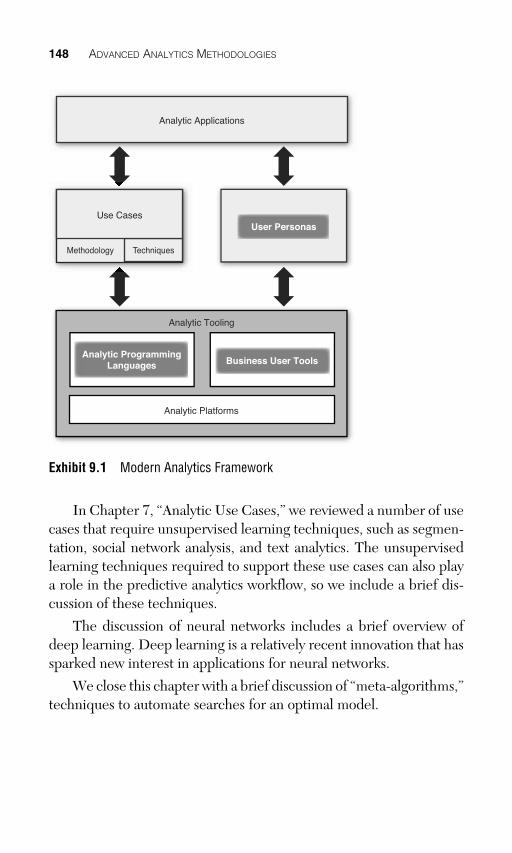
In this chapter, we review techniques that analysts use for predic-tive analytics. There are hundreds of different algorithms currently used to train predictive models; we do not claim to review these methods exhaustively but present a general description of “families” of techniques, together with an explanation of the strengths and weak-nesses for each family (see Exhibit 9.1 ).
Many statistical techniques are useful for both prediction and explanation. Some techniques, however, such as Mixed Linear Mod-els, are primarily useful for explanation, where the analyst seeks to assess the effect of one or more measures on another measure. The scope of this chapter does not include these techniques.
We begin the chapter with a brief discussion of two key “streams” of innovation in predictive analytics: statistics and machine learning. The distinction between these two streams is no longer as clear as it once was, because practitioners and advocates of each stream borrow from the other.
We also review the impact of Big Data. Some analysts argue that the Big Data phenomenon should have no impact on predictive ana-lytics; these analysts argue that the core methods of predictive analyt-ics do not change with the scale of the data. We disagree and therefore demonstrate specific ways in which Big Data can and will affect the techniques that analysts use.
148 ADVANCED ANALYTICS METHODOLOGIES
Analytic Applications
User Personas
Analytic Tooling
Analytic ProgrammingLanguages Business User Tools
Analytic Platforms
Methodology Techniques
Use Cases
Exhibit 9.1 Modern Analytics Framework
In Chapter 7 , “Analytic Use Cases,” we reviewed a number of use cases that require unsupervised learning techniques, such as segmen-tation, social network analysis, and text analytics. The unsupervised learning techniques required to support these use cases can also play a role in the predictive analytics workflow, so we include a brief dis-cussion of these techniques.
The discussion of neural networks includes a brief overview of deep learning. Deep learning is a relatively recent innovation that has sparked new interest in applications for neural networks.
We close this chapter with a brief discussion of “meta-algorithms,” techniques to automate searches for an optimal model.
CHAPTER 9 • PREDICTIVE ANALYTICS TECHNIQUES 149
Statistics and Machine Learning
There are two classes of techniques for predictive analytics with very different legacies: statistical methods and machine learning.
Statistical methods, such as linear regression, estimate the param-eters of mathematical models with known properties; the analyst seeks to test the hypothesis that the behavior of interest conforms to a specific class of mathematical model. The advantage of these models is that they are highly generalizable. If you can demonstrate that his-torical data conforms to a known distribution, you can use this infor-mation to predict behavior for new cases.
For example, if you know the position, velocity, and acceleration of an artillery shell, you can predict where it will land because you can use a mathematical model to compute the point of impact. By analogy, if you can show that response to a marketing campaign fol-lows a known statistical distribution, you can predict response with a degree of confidence based on information about the customer’s past purchases, demographics, characteristics of the offer, and so forth.
The principal disadvantage of statistical methods is that real-world phenomena frequently do not conform to known statistical distributions.
Machine learning techniques differ fundamentally from statisti-cal techniques because they do not start from a particular hypothesis about behavior; instead, they seek to learn and describe the relation-ship between historical facts and target behavior as closely as possible. Because machine learning techniques are not constrained by specific statistical distributions, they are often able to build models that are more accurate.
However, machine learning techniques can overlearn, which means they learn relationships in the training data that cannot gen-eralize to the population. Consequently, most widely used machine learning techniques have built-in mechanisms to control overlearn-ing, such as cross-validation or pruning on an independent sample.
The distinction between statistics and machine learning is getting smaller, as the two fields converge; for example, stepwise regression is a hybrid method based on both traditions.

150 ADVANCED ANALYTICS METHODOLOGIES
The Impact of Big Data
By “Big Data,” we mean data sets that are “big” on any one of three dimensions: volume, variety, and velocity. One of the prem-ises of this book is that Big Data technology has already changed the analytics landscape and that a new approach is needed—what we call “Modern Analytics.”
How big is “Big?” For data management, data is Big Data if it is too large to fit efficiently in a relational database. For analytics, we use a different definition; data qualifies as Big Data if it meets any one of three conditions:
1. The analytic data set is too large to fit into memory on a single machine.
2. The analytic data set is too large to move to a dedicated analysis platform.
3. Source data for analysis resides in a Big Data repository, such as Hadoop, an MPP database, NoSQL database, or NewSQL database.
Data volume can mean two different things with different impli-cations for the analyst. When the analyst works with structured data in matrices or tables, “volume” can mean more rows, more columns, or both. Analysts routinely work with data sets containing millions or billions of rows by sampling records at random 1 and then using the sample to train and validate predictive models. Sampling works rea-sonably well when the goal is to build a single predictive model for the entire population and the incidence of modeled behavior is relatively high and uniform in the population. With modern analytics technol-ogy, however, sampling is an option and not a requirement forced on the analyst by limited computing resources.
Adding more columns to the analytic data set affects the analyst in a very different way. The most effective way to improve the perfor-mance of predictive models is to add new variables with information value; however, you cannot always know in advance what variables
1 Sampling is built into SAS’ SEMMA methodology.
CHAPTER 9 • PREDICTIVE ANALYTICS TECHNIQUES 151
will add value to a model. This means that as you add variables to the analytics data set, you need tooling that will enable the analyst to scan across many variables quickly to find those that add value to a predic-tive model.
Having many columns or variables also means that there are many possible ways to specify a predictive model. To illustrate this point, consider the simple example of an analytics data set with one response measure and five predictors—a tiny data set by any measures. There are 29 unique combinations of the five predictors as main effects and many other possible model specifications if you consider interaction effects and various transformations of the predictors. The number of possible model specifications explodes as the number of variables increases; this places a premium on methods and techniques that enable the analyst to search efficiently for the best model.
“Variety” means working with data that is not structured in matrix or table form. In itself, this is not new; analysts have worked with data in many different formats for years, and text mining is a mature field. The most important change introduced by the Big Data trend is the large-scale adoption of unstructured formats for analytic data stores and the growing recognition that unstructured data—web logs, medi-cal provider notes, social media comments, and so on—offers signif-icant value for predictive modeling. This means that analysts must consider unstructured data sources when planning projects and build the necessary tooling into enterprise analytics architecture.
“Velocity,” the third V of Big Data, affects predictive analytics in two ways: as source and as target. Analysts working with streaming data, such as telemetry from a racing car or live feeds from moni-toring equipment in a hospital intensive care unit, must use special techniques to sample and window the data stream; these techniques convert the continuous stream into a discrete time series for analysis.
When the analyst seeks to apply predictive analytics to streaming data, as in real-time scoring, most organizations will use a dedicated decision engine designed to deliver high performance when scoring individual transactions.
152 ADVANCED ANALYTICS METHODOLOGIES
Supervised and Unsupervised Learning
In Chapter 7 , we reviewed a number of analytic use cases, includ-ing text and document analytics, clustering, association, and anomaly detection. These use cases differ from the predictive modeling use case because there is no predefined response measure; the analyst seeks to identify patterns but does not seek to predict or explain a specific relationship. These use cases require unsupervised learning techniques.
Unsupervised learning refers to techniques that find patterns in unlabeled data, or data that lacks a defined response measure. Exam-ples of unlabeled data include a bit-mapped photograph, a series of comments from social media, and a battery of psychographic data gathered from a number of subjects. In each case, it may be possible to classify the objects through an external process: For example, you can ask a panel of oncologists to review a set of breast images and classify them as possibly malignant (or not), but the classification is not a part of the raw source data. Unsupervised learning techniques help the analyst identify data-driven patterns that may warrant fur-ther investigation.
Supervised learning, on the other hand, includes techniques that require a defined response measure. Not surprisingly, analysts primarily use supervised learning techniques for predictive analyt-ics. However, in the course of a predictive analytics project, analysts may use unsupervised learning techniques to understand the data and to expedite the model building process. Unsupervised learning techniques frequently used within the predictive modeling process include anomaly detection, graph and network analysis, Bayesian Networks, text mining, clustering, and dimension reduction.
Anomaly Detection
An analyst working on a supermarket chain’s loyalty card spend-ing data noticed an interesting pattern: Some customers appeared to spend exceptionally large amounts. These “supercustomers”—of whom there were no more than several dozen—accounted for

CHAPTER 9 • PREDICTIVE ANALYTICS TECHNIQUES 153
a disproportionate percentage of total spending. The analyst was intrigued: Who were these supercustomers? Did it make sense to develop a special program to retain their business (in the same way that casinos target “whales”)?
On deeper investigation—a process that took considerable digging—the analyst discovered that these “supercustomers” were actually store cashiers who swiped their own loyalty cards for custom-ers who did not have a card.
In Chapter 8 , “Predictive Analytics Methodology,” we noted that analysts investigate and treat outliers as they develop the analysis data set. They do this for two reasons: First, because outliers can make it very difficult to fit a predictive model to the data at all; and second, because outliers may indicate a problem with the data, as the super-market analyst learned.
As a rule, the analyst should remove outliers from the analysis data set only when they are artifacts of the data collection process (as is the case in the supermarket example). Investigating outliers can take a considerable amount of time; thus, the analyst needs formal methods to identify anomalies in the data as quickly as possible.
In many cases, simple univariate methods will suffice. For univari-ate anomaly detection, the analyst runs simple statistics on all numeric variables. The process flags records with values that exceed defined minima or maxima for each variable, and flags records whose values exceed a defined number of standard deviations from the mean. For categorical variables, the analyst compares the variable values with a list of acceptable values, flagging records with values not included in the list. For example, in a data set that represents customers who reside in the United States, a “State” variable should include only 51 acceptable values; records with any other value in this field require analyst review.
Univariate methods for anomaly detection may miss some unusual patterns. To take a simple example, consider the case of a person who measures 74 inches tall and weighs 105 pounds. Neither the height nor the weight of this person is exceptional, but the combination of the two is highly unusual and rare. Analysts use multivariate anomaly

154 ADVANCED ANALYTICS METHODOLOGIES
detection techniques to identify these unusual cases. Multiple tech-niques are available to the analyst, including clustering techniques (see later in this chapter), single-class support vector machines, and distance-based techniques (such as K-nearest neighbors). These tech-niques are useful when anomaly detection is the primary goal of the analysis (as is the case for security and fraud applications); however, they are rarely used in the predictive analytics process.
Graph and Network Analysis
In Chapter 7 , we discussed the graph analysis use case, a form of discovery with proven value in social media analysis, fraud detection, criminology, and national security. Mathematical graphs do not play a direct role in predictive analytics but can play a supporting role in two ways.
First, graphs are very useful in exploratory analysis, where the analyst simply seeks to understand behavior. Bayesian belief net-works, discussed next, are a special case of graph analysis, where the nodes of the graph represent variables. However, an analyst can gain valuable insights from other applications of graph analysis, such as social network analysis. In a social graph, the nodes represent per-sons, and edges represent relationships among persons; using a social graph, a criminologist discovered that most murders in Chicago took place within a very small social network. 2 This insight can lead the analyst to examine the characteristics that distinguish the high-risk social network and a model that predicts homicide risk.
Graph analysis can also contribute features to a predictive model based on a broader set of data. For example, the social distance between a prospective customer and an existing customer—derived from a social graph—could be a strong feature in a model that pre-dicts response to a marketing offer. As another example, the number of social links between an employee and other employees might be a valuable predictor in an employee retention model.
2 Whet Moser, “The Small Social Networks at the Heart of Chicago Violence,” December 9, 2013, http://www.chicagomag.com/city-life/December-2013/The-Small-Social-Networks-at-the-Heart-of-Chicago-Violence/ .

CHAPTER 9 • PREDICTIVE ANALYTICS TECHNIQUES 155
Bayesian Networks
Bayesian inference is a formal system of reasoning that reflects something you do in everyday life: use new information to update your beliefs about the probability of an event. For an example of this kind of reasoning, consider a sales associate at a car dealer who must decide how much time to spend with “walk-in” customers. The sales associate knows from experience that only a very small percentage of these customers will buy a car, but he also knows that if the customer currently owns the brand of car sold at the dealership, the odds of a purchase increase significantly. Using a form of Bayesian inference, the sales associate asks each “walk-in” customer what he or she cur-rently drives and then uses this information to qualify the customer accordingly.
Suppose that you have a great deal of data about an entity, and you want to understand what data is most useful for predicting a par-ticular event. For example, you may be interested in modeling loan defaults in a mortgage portfolio and have copious data about the bor-rower, mortgaged property, and local economic conditions. Bayesian methods help you identify the information value of each data item so that you can focus attention on the most important predictors.
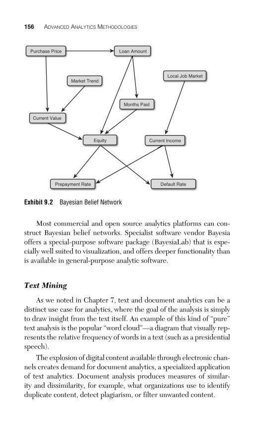
A Bayesian belief network represents a system of relationships among variables through a mathematical graph (described in the pre-ceding section). A belief network represents variables as nodes in the graph and conditional dependencies as edges, as shown in Exhibit 9.2 .
Belief networks are highly interpretable; modeling and visualiz-ing a belief network helps the analyst understand relationships among a large set of variables and form hypotheses about the best ways to model those relationships. The belief network models the system as a whole and does not categorize variables as “predictor” and “response” measures. Hence, it is a valuable tool to explore the data while work-ing with a business stakeholder to define the predictive modeling problem. (We discuss Bayesian methods for predictive modeling later in this chapter.)
156 ADVANCED ANALYTICS METHODOLOGIES
Most commercial and open source analytics platforms can con-struct Bayesian belief networks. Specialist software vendor Bayesia offers a special-purpose software package (BayesiaLab) that is espe-cially well suited to visualization, and offers deeper functionality than is available in general-purpose analytic software.
Text Mining
As we noted in Chapter 7 , text and document analytics can be a distinct use case for analytics, where the goal of the analysis is simply to draw insight from the text itself. An example of this kind of “pure” text analysis is the popular “word cloud”—a diagram that visually rep-resents the relative frequency of words in a text (such as a presidential speech).
The explosion of digital content available through electronic chan-nels creates demand for document analytics, a specialized application of text analytics. Document analysis produces measures of similar-ity and dissimilarity, for example, what organizations use to identify duplicate content, detect plagiarism, or filter unwanted content.
Default RatePrepayment Rate
Current Value
Equity
Purchase Price
Market Trend
Months Paid
Local Job Market
Loan Amount
Current Income
Exhibit 9.2 Bayesian Belief Network

CHAPTER 9 • PREDICTIVE ANALYTICS TECHNIQUES 157
In predictive analytics, text mining plays a supplemental role: Ana-lysts seek to enhance models by incorporating information derived from text into a predictive model that may capture other information about the subject. For example, a hospital seeking to predict read-mission among discharged patients relied on a battery of quantita-tive measures such as diagnostic codes, days since first admission, and other characteristics of the treatment; it was able to improve the model by adding predictors derived from practitioners’ notes with text mining. Similarly, an insurance carrier was able to improve its ability to predict customer attrition by capturing data from call center notes.
The most common form of text mining depends on word counting, but the task is more complicated than simply counting the incidence of each unique word. The analyst must first clean and standardize the text by correcting spelling errors; removing common words such as the, and, or, and so forth; stemming, or reducing inflected and derived words to their root; and employing other methods that remove noise from the text.
Word counting begins when the text is clean. Two distinctly different methods are in common usage. The simplest method just counts the incidence of each unique word in each document; for example, in the hospital case, the word-counting algorithm counts the incidence of unique words in each patient’s record. The output of this process is a sparse matrix with one column for each distinct word, one row for each document, and values in the cells representing the word count. This matrix is impossibly large to use in a predictive model in its raw form, so the analyst applies dimension-reduction techniques to reduce the word count matrix to a limited number of uncorrelated dimensions. (See the section on dimension reduction later in this chapter.)
A second method counts associations rather than words. For example, the algorithm counts how often two words appear together within a sliding window of n words, within a sentence or within a paragraph. The output of this process is a “words by words” matrix, to which the analyst applies dimension-reduction techniques. This method can produce insights with relatively small quantities of text, but it requires a scoring process to assign feature values to each record in the raw data.
158 ADVANCED ANALYTICS METHODOLOGIES
Clustering
As we discussed in Chapter 7 , segmentation is one of the most effective and widely used strategic tools available to businesses today. Strategic segmentation is a business practice that depends on an ana-lytic use case (market segmentation or customer segmentation); the use case, in turn, depends on a set of unsupervised learning tech-niques called clustering .
Clustering techniques divide a set of cases into distinct groups that are homogeneous with respect to a set of variables we call the active variables . In customer segmentation, each case represents a customer; in market segmentation, each case represents a consumer who may be a current customer, a former customer, or a prospec-tive customer. Of course, you can use clustering techniques in other domains aside from customer and market segmentation.
Although strategic segmentation is a distinct analytic use case, segmentation can also play a tactical role in predictive analytics. As a rule, analysts can improve the overall effectiveness of a predictive model by splitting the population into subgroups, or segments, and modeling separately for each segment. In some cases, the subgroups are logically apparent and easily identified without formal analysis. Suppose, for example, that a credit card issuer wants to build a model that will predict delinquency in the next 12 months. The model likely includes predictors based on the cardholder’s transacting and pay-ment behavior over some finite period (such as the prior 12 months). Cardholders acquired less than 12 months ago will have incomplete data for these predictors; consequently, it may make sense to seg-ment the cardholder base into two groups: those acquired at least 12 months ago and those acquired less than 12 months ago. The analyst then builds separate predictive models for each group of card holders. (In actual practice, credit card issuers subdivide their portfolios into many such segments for risk modeling based on a range of character-istics, including cardholder tenure, type of card product, country of issue, and so forth.)
The practice described in the preceding paragraph is a priori seg-mentation, where the analyst knows the desired segmentation scheme

CHAPTER 9 • PREDICTIVE ANALYTICS TECHNIQUES 159
in advance. When the analyst does not know the optimal segmenta-tion scheme in advance, clustering techniques help the analyst seg-ment the analysis data set into homogeneous groups. A bookstore, for example, might have data about customer spending across a wide range of categories. Running a cluster analysis reveals (hypothetically) five distinct groups of customers:
• High-spending customers who buy in many categories
• High-spending customers who buy fiction only
• Medium-spending customers who buy mostly children’s books
• Medium-spending customers who buy books on military his-tory, sports, and auto repair
• Light-spending customers
This clustering has business value in its own right, but it also enables the analyst to build distinct predictive models for each segment.
You can use many techniques for clustering; the most widely used is k-means clustering, a technique that minimizes the variation from the cluster mean for all active variables. The standard k-means algo-rithm is iterative and relies on random seed values; the analyst must specify the value of k, or the number of clusters. There are many vari-ations on k-means, including alternative computational methods, and a range of enhancements in software implementations; these include capabilities to visualize and interpret the clusters, and “wrappers” that help the analyst determine the optimal number of clusters.
K-means clustering is available in most commercial data min-ing packages (together with other clustering methods). Open source options include the k-means package in R (among many others) and scikit-learn in Python. To be useful as a segmentation tool, clustering must run on the entire population; hence, leading database vendors such as IBM, PureData (Netezza), and Oracle have built-in capability for k-means, and leading in-database libraries support the capabil-ity as well. In Hadoop, open source implementations are included in Apache Mahout, Apache Spark, and independent platforms such as H2O.

160 ADVANCED ANALYTICS METHODOLOGIES
Dimension Reduction
Analysts tend to use the words dimension, feature, and predictor variable interchangeably. Although each term has a precise meaning in academic literature, in this section we treat them as synonymous and address the practical problems posed by data sets with a very large number of predictors.
An in-depth treatment of dimensionality and its impact on the techniques reviewed in this chapter is out of scope for this book. Suf-fice it to say that high dimensionality complicates predictive modeling in two ways: through added computational complexity and runtime, and through the potential to produce a biased or unstable model. In this context, there is no simple rule that defines “large.” On the one extreme, problems in image recognition or genetics may have millions of potential predictors, but with some methods, analysts encounter issues with as few as a thousand or several hundred predictors.
Analysts use two types of techniques to reduce the number of dimensions in a data set: feature extraction and feature selection. As the name suggests, feature extraction methods synthesize informa-tion from many raw variables into a limited number of dimensions, extracting signal from noise. Feature selection methods help the ana-lyst choose from a number of predictors, selecting the best predictors for use in the finished model and ignoring the rest.
The most popular technique for feature extraction is principal component analysis, or PCA. First introduced in 1901, PCA is widely used in the social sciences and marketing research; for example, consumer psychologists use the method to draw insights from large batteries of attitudinal data captured in surveys. PCA uses linear alge-bra to extract uncorrelated dimensions from the raw data. Although the method is well established and relatively easy to implement, it assumes the data are jointly normally distributed, a condition that is often violated in commercial analytics. Variations on PCA include Kernel PCA and Multilinear PCA; there is also a wide range of other advanced methods for feature extraction. Most commercial analytics packages implement PCA; alternatives to PCA are available in open source software.
Many predictive modeling techniques have built-in feature selec-tion capabilities: The technique automatically evaluates and selects

CHAPTER 9 • PREDICTIVE ANALYTICS TECHNIQUES 161
from available predictors. These techniques include tree-based meth-ods (such as CART or C5.0); boosted methods (such as ADABoost); bootstrap aggregation, or bagging; regularized methods, such as LARS or LASSO; and stepwise methods. When the modeling tech-nique has built-in feature selection, the analyst can omit the feature selection step from the modeling process; this is a key reason to use these methods.
When the analyst does not want to use a technique with built-in feature selection, several options are available. The analyst can run a forward stepwise procedure (see “Stepwise Regression” later in this chapter) with a low threshold for variable inclusion; this will produce a list of candidate predictors, which the analyst can fine-tune in a second step. Another popular method for feature selection is to run regularized random forests (RRF) analysis, which produces a set of nonredundant variables.
Previously in this chapter, we discussed the value of Bayesian belief networks for exploratory analysis. After building a belief net-work, the analyst can use it for feature selection. Recall that each node in a belief network represents a variable in the analytic data set. For any given target node (the response measure), the Markov blanket consists of all the parent and child nodes that make this node independent of all other nodes in the network.
Whereas feature extraction is more elegant than feature selection and has a long history of academic use, feature selection is the more practical tool. On one hand, feature extraction techniques such as PCA add an additional step to the scoring process, which must score and convert raw data to the principal dimensions before computing a score. On the other hand, predictive models based on feature selec-tion techniques work with data as it exists in production (assuming the analyst worked with data in its raw form).
Linear Models and Linear Regression
Linear models and linear regression techniques are the most fun-damental methods available to the analyst for predictive modeling; we review these methods next.
162 ADVANCED ANALYTICS METHODOLOGIES
Basics: Linear Models
A mathematical model is an expression that describes the rela-tionship between two or more measures. Businesses use models in many ways—pricing is a familiar example. If the price of one widget is five dollars, the price of many widgets is y = 5* x , where y is the total price quoted and x is the number of widgets bought. If you express pricing as a mathematical model, you can build the model formula into point-of-sale devices, online quote systems, and a host of other useful applications. (Of course, because organizations set prices for their products, you don’t need a statistician to discover the pricing model; you can simply call the Pricing department. We’re just using pricing as an everyday example.)
A linear model is a mathematical model in which the relationship between an independent variable and the dependent variable is con-stant for all values of the independent variable. In other words, if y = 2 x when x = 2, this formula will also be true if x = 4, x = 4,000,000, or any arbitrary value.
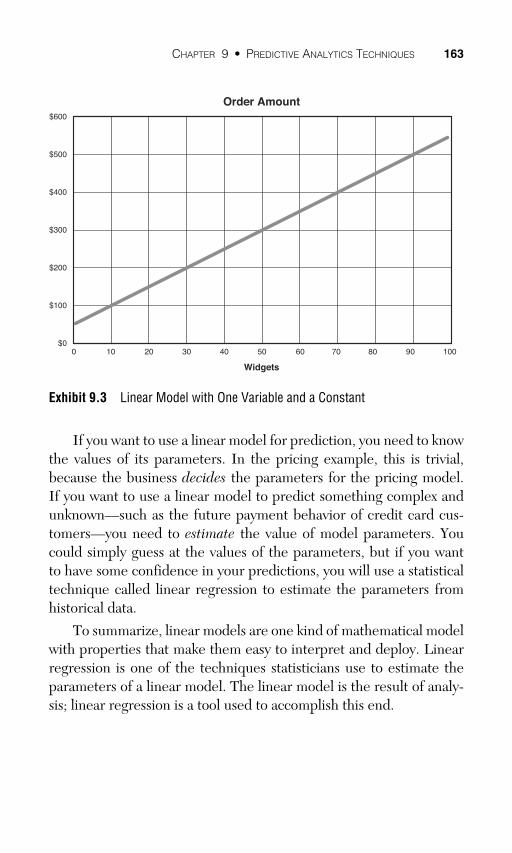
A linear model can also include a constant. Suppose that the pric-ing includes a shipping and handling fee of 50 dollars; now, the pric-ing model is y = 50 + 5* x . It is easy to visualize a linear model with a single variable and a constant (see Exhibit 9.3 ).
A linear model can include more than one predictor as long as the predictors are additive. For example, if the price of a gadget is two dollars, the total price of an order is y = 50 + 5* x 1 + 2* x 2, where x 1 is the number of widgets and x 2 is the number of gadgets. You can extend this model to include any number of items as long as the total quote is simply the sum of the quote for individual items plus a constant.
Generalizing from the pricing example, a linear model is one that you can express as y = b + a 1 x 1 + a 2 x 2 + ... + anxn, where y is the response measure and x 1... xn are the predictors. Statisticians call the remaining values in the equation parameters ; they include the value of b , a constant, and the values a 1 through an, called coefficients . The coefficients represent the relationship between the predictors and the response measure; when there is a single predictor, this is the slope of a line representing the function.
CHAPTER 9 • PREDICTIVE ANALYTICS TECHNIQUES 163
If you want to use a linear model for prediction, you need to know the values of its parameters. In the pricing example, this is trivial, because the business decides the parameters for the pricing model. If you want to use a linear model to predict something complex and unknown—such as the future payment behavior of credit card cus-tomers—you need to estimate the value of model parameters. You could simply guess at the values of the parameters, but if you want to have some confidence in your predictions, you will use a statistical technique called linear regression to estimate the parameters from historical data.
To summarize, linear models are one kind of mathematical model with properties that make them easy to interpret and deploy. Linear regression is one of the techniques statisticians use to estimate the parameters of a linear model. The linear model is the result of analy-sis; linear regression is a tool used to accomplish this end.
Order Amount
Widgets
$600
$500
$400
$300
$200
$100
$00 10 20 30 40 50 60 70 80 90 100
Exhibit 9.3 Linear Model with One Variable and a Constant

164 ADVANCED ANALYTICS METHODOLOGIES
Basics: Linear Regression
When you do not know the parameters of a hypothetical linear model in advance, linear regression is the method you use to estimate those parameters. Linear regression scans the data and computes parameters for the linear model that “best” fits the data. The method chooses an optimal model through the least squares criterion, which minimizes the squared errors between predicted and actual values.
Suppose that you are interested in predicting the total crop yield from small farms, and you believe that the number of acres in produc-tion is the single most important predictor of total yield. (The farms are all in the same general area and use similar practices.) When you plot total yield against acres in production for a sample of 100 farms, you get the graph like the one shown in Exhibit 9.4 . The dashed line is the linear regression line.
Farm Yield (Bushels)
Acres
2,000
1,800
1,600
1,400
1,200
1,000
800
600
400
200
-0 10 20 30 40 50 60 70 80 90 100
y = 9.9734x + 479.94R2 = 0.5184
Exhibit 9.4 Linear Regression
Linear regression is a powerful and widely used method that is pervasive in statistical packages and relatively easy to implement. However, the method has a number of properties that limit its appli-cation, require the analyst to prepare the data in certain ways or, in the worst case, lead to spurious results.
Among the limiting factors, the most important is an assumption that the response measure is a continuous numeric variable. Although

CHAPTER 9 • PREDICTIVE ANALYTICS TECHNIQUES 165
it is possible to fit a regression model to a categorical response mea-sure, the results are likely to be inferior to what the analyst could achieve using methods designed for categorical response measures, which we discuss in a later section.
Two characteristics of regression require the analyst to take addi-tional steps to prepare the data. Like most statistical methods, regres-sion requires that all fields specified in the model have a value, and will remove records with missing values from the analysis. Regression also requires continuous numeric predictors. Analysts can work around the missing data problem through exhaustive quality control when gathering data, or by imputing values for missing fields. Analysts can also handle categorical variables in linear regression through a method called dummy coding . Statistical software packages vary widely in the degree to which they automate these tasks for the analyst.
Analysts are most concerned with those characteristics of linear regression that produce an inferior or spurious model. For example, linear regression presumes that a linear model is the appropriate the-oretical model to represent the behavior you seek to analyze. The point is important because the regression algorithm does not know the true theoretical model and will attempt to estimate model param-eters from data regardless of the true state of affairs. Exhibit 9.5 shows an example of a spurious relationship.
Random Variable Y
Random Variable X
10,000
9,000
8,000
7,000
6,000
5,000
4,000
3,000
2,000
1,000
-0 10 20 30 40 50 60 70 80 90 100
y = -14.083x + 5637.5R2 = 0.0222
Exhibit 9.5 Chart Showing Spurious Regression Line

166 ADVANCED ANALYTICS METHODOLOGIES
The analyst detects a weak model by inspecting model diagnos-tics. However, it is theoretically possible for a regression model to identify a statistically significant relationship between two variables when no causal relationship exists between them in the real world.
For each model specification, linear regression packages report a key statistic called the coefficient of determination, or R-squared. This statistic measures how well the model fits the data; conceptually, it measures variation in the response measure explained by the model as a percentage of the total variation in the response measure. Ana-lysts use this measure together with its associated F-test to determine the quality of the model. If the R-squared is low, the analyst will look for ways to improve the model, either by adding more predictors or by using a different method.
Analysts also examine the significance tests for each model coef-ficient. If a coefficient fails a significance test, the implication is that its true value is zero, and the associated predictor does not meaning-fully contribute to the model. Good modeling practice calls for drop-ping this predictor from the model specification and re-estimating the model.
If two or more predictors are highly correlated, estimated values of the coefficients can be highly unstable. This condition, known as multicollinearity, does not impair the overall ability of the model to predict, but it renders the model less useful for explanatory analysis.
Advantages and Disadvantages
The principal advantage of linear regression is its simplicity, inter-pretability, scientific acceptance, and widespread availability. Linear regression is the first method to use for many problems. Analysts can use linear regression together with techniques such as variable recod-ing, transformation, or segmentation.
Its principal disadvantage is that many real-world phenomena simply do not correspond to the assumptions of a linear model; in these cases, it is difficult or impossible to produce useful results with linear regression.
Linear regression is widely available in statistical software pack-ages and business intelligence tools.

CHAPTER 9 • PREDICTIVE ANALYTICS TECHNIQUES 167
Generalized Linear Models
Standard linear models assume that the response measure is nor-mally distributed and that there is a constant change in the response measure for each change in predictor variables. In many real-world situations, however, this assumption is inappropriate, and a linear model may be unreliable.
For example, suppose that you want to model how weekly in-store sales of an item respond to targeted coupons. A linear model might tell you that sales per store increase by a thousand units for each one-dollar decrease in the net price. However, when you inspect the pre-diction errors for this model, you find that the model significantly overestimates the incremental sales for stores that typically sell only a thousand units a week, and significantly underestimates incremental sales for stores that typically sell ten thousand units a week or more.
Based on analysis of the errors from the linear model, the ana-lyst reformulates the model to predict the percentage change in store sales based on changes in the net price. In other words, the analyst changes the model from a linear response model to an exponential or log-linear response model. Generalized linear models provide the necessary flexibility to make this change.
Whereas standard linear models require a normally distributed response measure, generalized linear models work effectively with many different distributions. Moreover, while linear models assume a linear relationship between the predictors and the response measure, generalized linear models simply assume this relationship is linear when transformed by a link function.
With generalized linear models, the analyst specifies three things: a probability distribution that describes the response measure, a link function that describes the relationship between the predictors and the mean of the response measure, and a set of linear predictors. Probability distributions can include any member of the exponential family, including the Bernoulli, Beta, Chi-squared, Dirichlet, Expo-nential, Gamma, Normal, Poisson, and Wishart distributions.
Generalized linear models are more demanding for the ana-lyst due to the number and complexity of controllable parameters.
168 ADVANCED ANALYTICS METHODOLOGIES
Software implementations of GLM often include diagnostic tools to help the analyst diagnose the appropriate distribution for the response measure and recommend a link function.
Generalized Additive Models
The generalized additive model (GAM) is a type of nonparamet-ric regression. Techniques such as linear regression are parametric , which means they incorporate certain assumptions about the data. When an analyst uses a parametric technique with data that does not conform to its assumptions, the result of the analysis may be a weak or biased model. Nonparametric regression relaxes assumptions of linearity, enabling the analyst to detect patterns that parametric tech-niques may miss.
There are a number of different nonparametric techniques, but many of them perform poorly with many potential predictors; they tend to be greedy for large sample sizes and may lack stability. Certain methods, such as kernel methods and smoothing splines, are also very difficult to interpret.
The additive model, first proposed in the early 1980s, is a more general form of the linear regression model, which you express as y = b + a 1 x 1 + a 2 x 2 + ... + anxn. In an additive model, you replace the simple terms of the linear equation with more complex functions. In a generalized additive model, the regression equation takes the form of a link function so that the response measure can take the form of any of the family of exponential distributions.
The principal advantage of GAM is its ability to model highly complex nonlinear relationships when the number of potential pre-dictors is large. The main disadvantage of GAM is its computational complexity; like other nonparametric methods, GAM has a high pro-pensity for overfitting.
SAS, Statistica, and Stata all support GAM. There are 17 differ-ent packages in open source R that support GAM, but none currently available in Python.
CHAPTER 9 • PREDICTIVE ANALYTICS TECHNIQUES 169
Logistic Regression
Linear regression is powerful and widely used. In real-world appli-cations, however, analysts often seek to model categorical behavior:
• Prospects either respond or do not respond to a marketing communication.
• Borrowers repay a loan or do not repay a loan.
• Shoppers choose Brand X over Brand Y and Brand Z.
It is frequently possible to model this behavior with linear regres-sion by coding the response measure as 1 (if the prospect responds) and 0 (if the prospect does not respond), but another technique called logistic regression produces better and more useful results. Statisti-cians developed logistic regression specifically to model the rela-tionship between a categorical dependent variable and one or more response measures. As with linear regression, the predictors are ordi-narily continuous, but experienced analysts work around this require-ment through dummy coding.
Analysts use logistic regression to address three types of classi-fication problems. The first is binomial classification, in which the response measure has only two levels: a prospect either responds or does not respond. A second type of classification problem is multino-mial ordinal classification, in which the response measure can have more than two values, but there is an implied rank ordering: surveyed customers report that they are “very satisfied,” “somewhat satisfied,” “somewhat dissatisfied,” or “very dissatisfied.” The third type of clas-sification problem is multinomial cardinal classification, in which the response measure can have more than two values and there is no implied rank ordering: surveyed customers can choose among “Chev-rolet,” “Ford,” “Honda,” and “Toyota.”
Logistic regression produces estimates of the model intercept and coefficients, together with quality statistics for the individual param-eters and the model as a whole. When applied to new data, the logistic regression produces a probability ranging from zero to one reflecting

170 ADVANCED ANALYTICS METHODOLOGIES
the relative likelihood that the case belongs to the target class, given the known values of predictor variables. For use in decision making, the analyst uses this predicted probability together with a cutoff rule to classify each new case.
The most widely used method to estimate logistic regression models is the maximum likelihood algorithm. Maximum likelihood is an iterative algorithm; it assigns initial values to the model coef-ficients, tests the initial solution against training data, improves the model, and iterates, improving and testing until it can find no more improvements. Software implementations of logistic regression gen-erally offer the analyst the ability to specify details of the model qual-ity measure, significance thresholds for model improvements, and total number of iterations.
In some cases, the maximum likelihood algorithm reaches the maximum number of iterations before it can find a meaningful solu-tion. This can happen when predictors are highly correlated, with sparse matrices, or when the number of predictors is very large rela-tive to the number of cases. Analysts address the problem of corre-lated predictors with dimension-reduction techniques, which they apply to the data before running logistic regression. There are tech-niques for use with sparse matrices and high dimension data; we dis-cuss each separately.
Almost all commercial statistical packages offer an implementa-tion of logistic regression. The method is also widely available in open source versions, with more than 50 versions available in open source R alone.
Enhanced Regression
As the volume of data grows, analysts struggle to work with data sets containing large numbers of potential predictors. Expanding the number of candidate predictors poses technical issues for ana-lytic algorithms, increases the demands for computing resources, and poses potential methodological problems for the analyst. Analysts consider a number of mathematical transforms for predictors as well as interaction effects among predictors; consequently, the number of

CHAPTER 9 • PREDICTIVE ANALYTICS TECHNIQUES 171
measures actually used in the predictive model expands exponentially as the number of raw candidate measures increases.
There are two widely used methods to address this problem: step-wise methods and regularization. We discuss these methods next.
Stepwise Regression
Stepwise regression is a hybrid method that combines statistical modeling with machine learning techniques. Recall that in the previ-ous discussion on linear regression, we noted that the analyst specifies a model, estimates the model, inspects the significance tests for the coefficients, and respecifies the model to remove nonsignificant pre-dictors. This process of constructing a model works reasonably well with a limited number of possible predictors but takes a considerable amount of time when there is a large number of predictors.
Stepwise regression methods streamline the model-building task by automating the process. Three approaches to automation are used widely:
• Forward selection — The algorithm begins with an (optional) intercept-only model and progressively adds candidate predic-tors until it reaches a stopping point.
• Backward selection — The algorithm begins with a model that includes all candidate predictors and progressively eliminates them from the model until it reaches a stopping point.
• Bidirectional stepwise — The algorithm proceeds similar to forward selection, but at each step, it can either add or drop candidate predictors until it reaches a stopping point.
Stepwise algorithms evaluate candidate predictors by compar-ing two versions of the model: one that includes the predictor and another that does not include the predictor. The algorithm performs a statistical test to select one of the two candidate models; in most software implementations, the user can select the test criterion. The three most widely used measures are the F-test, Aikaike’s information criterion (AIC), and the Bayesian information criterion (BIC).

172 ADVANCED ANALYTICS METHODOLOGIES
Although stepwise regression is efficient and effective for pre-dictive modeling, the method is less useful for analysis of variance, in which there is a premium on analytic rigor and statistical validity. Stepwise regression is also subject to overfitting, in which the model produced does not generalize well from the training data to produc-tion data (for more on overfitting, see the next section). For these reasons, many analysts use stepwise regression primarily as an explor-atory tool to narrow the set of possible predictors.
Stepwise regression methods work with any underlying form of regression; the most popular are stepwise linear and stepwise logistic regression.
Regularization
Overfitting or overlearning is a condition in which the accuracy of a model is much higher on its training data set than on an indepen-dent data set. In short, the model does not generalize well because the algorithm that produced it learned random features of the train-ing data. This is a serious problem for analysts because the ultimate test of a model is how it performs in production, not how well it per-forms in the lab.
As a rule, overfitting is a larger problem for machine learning than statistics because statistical models have a foundation in known statis-tical distributions. However, as the complexity of a model increases and additional predictors are added, even statistical models can suffer from overfitting.
There are several techniques to prevent overfitting, including validation of the model on an independent sample, n-fold cross-validation, and regularization. We cover the first two under machine learning; in this section, we discuss regularization.
Regularization methods limit complexity by penalizing models based on the number of predictors. To enter into the model, each new candidate predictor must overcome a progressively higher com-plexity penalty. There are several specific methods for regulariza-tion; the most widely used are ridge regression (also called Tikhonov regularization or constrained linear inversion) and LASSO regression

CHAPTER 9 • PREDICTIVE ANALYTICS TECHNIQUES 173
(or least absolute shrinkage and selection operator). The Elastic Net method combines ridge and LASSO regularization.
Higher-end statistical software generally includes ridge and lasso regularization, and so does open source R. For Elastic Net, Math-Works offers a commercial implementation, and in open source R, the popular glmnet package supports the capability.
Survival Analysis
For some business applications, the response measure you want to predict is the elapsed time to an event. This can be literally a life-time, if you model human mortality for life insurance; or, it can be time to failure for a device, time to attrition for a customer account, or any other similar situation in which you want to predict survival.
Time-to-event measures pose unique problems for the analyst. Suppose that you want to predict the survival time for patients receiv-ing an experimental cancer treatment. After three years, some of the patients in the study have died, and you can compute the survival time for each of these patients. However, many of the patients are still living at the end of three years; you do not yet know their ultimate survival time. Statisticians call this problem censoring , a problem that surfaces when you try to model a time-to-event response measure using data captured over a limited time period.
The two kinds of censoring are right censoring and left censor-ing. If you only know that the pertinent event is after some date, as is the case for patients in the preceding example who survive to the end of the study, the data is right-censored. On the other hand, if you only know that the beginning of the pertinent time-to-event took place before a certain date, the data is left-censored. For example, if you know that every patient in the study received the experimental treatment before the study started but do not know the exact date of treatment, the data is left-censored. Data can be both right-censored and left-censored.
Survival analysis is a family of techniques developed to work with censored time-to-event response measures. Note that if censoring is

174 ADVANCED ANALYTICS METHODOLOGIES
not present, you may be able to model time-to-event using standard modeling techniques. For some studies, however, you would have to wait a very long time before every sampled observation has a ter-minal event; in the case of the experimental cancer treatment, some patients might live another 20 years. Hence, survival analysis tech-niques enable the analyst to take full advantage of available data with-out waiting until every treated patient dies, every sampled part fails, or every tracked account closes.
In addition to the censoring problem described previously, time-to-event response measures generally follow an exponential, or Weibull, distribution rather than a normal distribution; consequently, linear regression tends to perform poorly. Three alternative tech-niques are used widely for this problem:
• Cox’s proportional hazards model
• Exponential regression
• Log-normal regression
Cox’s proportional hazards (CPH) model is a nonparametric method, which means that it makes no assumptions about the distri-bution of the response measure. CPH models the underlying hazard rate (for example, risk of death) as a function of a baseline hazard rate and the incremental effects of predictor variables. Exponential regression assumes that the time-to-event response measure follows an exponential distribution. In log-normal regression, the analyst replaces the raw survival response measure with its natural logarithm and then uses standard regression tools to model the transformed measure. Log-normal regression is the simplest technique to imple-ment but may not perform as well as CPH or exponential regression.
Popular statistical packages (such as SAS, SPSS, and Statistica) support all three methods. There are many packages for survival anal-ysis in open source R.
Decision Tree Learning
Decision trees are a very popular tool for predictive analytics because they are relatively easy to use, perform well with non-linear
CHAPTER 9 • PREDICTIVE ANALYTICS TECHNIQUES 175
relationships and produce highly interpretable output. We discuss different methods for decision tree learning below.
Overview
Decision tree learning is a class of methods whose output is a list of rules that progressively segment a population into smaller seg-ments that are homogeneous in respect to a single characteristic, or target variable. End users can visualize the rules as a tree diagram, which is very easy to interpret, and the rules are simple to deploy in a decision engine. These characteristics—transparency of the solution and rapid deployment—make decision trees a popular method.
Readers should not confuse decision tree learning with the deci-sion tree method used in decision analysis, although the result in each case is a tree-like diagram. The decision tree method in deci-sion analysis is a tool that managers can use to evaluate complex decisions; it works with subjective probabilities and uses game theory to determine optimal choices. Algorithms that build decision trees, on the other hand, work entirely from data and build the tree based on observed relationships rather than the user’s prior expectations.
You can train decision trees with data in many ways; the sections that follow describe the most widely used methods. The Ensemble Learning section covers advanced methods (such as bagging, boost-ing, and random forests).
CHAID
CHAID (Chi-Square Automatic Interaction Detection) is one of the oldest tree-building techniques; in its most widely used form, the method dates to a publication by Gordon V. Kass in 1980 3 and draws on other methods developed in the 1950s and 1960s.
CHAID works only with categorical predictors and targets. The algorithm computes a chi-square test between the target variable and each available predictor and then uses the best predictor to partition
3 Kass, Gordon V., “An Exploratory Technique for Investigating Large Quantities of Categorical Data,” Applied Statistics, Vol. 29, No. 2 (1980).
176 ADVANCED ANALYTICS METHODOLOGIES
the sample. It then proceeds, in turn, with each segment and repeats the process until no significant splits remain. The standard CHAID algorithm does not prune or cross-validate the tree.
Software implementations of CHAID vary; typically, the user can specify a minimum significance of the chi-square test, a minimum cell size, and a maximum depth for the tree.
The principal advantages of CHAID are its use of the chi-square test (which is familiar to most statisticians) and its ability to perform multiway splits. The main weakness of CHAID is its limitation to cat-egorical data.
CART
CART, or Classification and Regression Trees, is the name of a patented application marketed by Salford Systems based on an epon-ymous 1984 publication by Leo Breiman. 4 CART is a nonparametric algorithm that learns and validates decision tree models.
Like CHAID, the algorithm proceeds recursively, successively splitting the data set into smaller segments. However, there are key differences between the CHAID and CART algorithms:
• CHAID uses the chi-square measure to identify split candi-dates, whereas CART uses the Gini rule.
• CHAID supports multiway splits for predictors with more than two levels; CART supports binary splits only and identi-fies the best binary split for complex categorical or continuous predictors.
• CART prunes the tree by testing it against an independent (validation) data set or through n-fold cross-validation; CHAID does not prune the tree.
CART works with either categorical targets (classification trees) or continuous targets (regression trees) as well as either categorical or continuous predictors. This is a key advantage of CART versus CHAID, together with its ability to develop more accurate decision
4 L Breiman, J Friedman, CJ Stone, RA Olshen, CRC press (1984).

CHAPTER 9 • PREDICTIVE ANALYTICS TECHNIQUES 177
tree models. The principal disadvantage of CART is its proprietary algorithm.
ID3/C4.5/C5.0
ID3, C4.5, and C5.0 are tree-learning algorithms developed by Ross Quinlan, an Australian computer science researcher.
ID3 (Iterative Dichotomiser) is similar to CHAID and CART, but uses the entropy or information gain measures to define splitting rules. ID3 works with categorical targets and predictors only.
C4.5 is a successor to ID3, with several improvements. C4.5 works with both categorical and continuous variables, handles missing data, and enables the user to specify the cost of errors. The algorithm also includes a pruning function. C5.0, the most current commercial version, includes a number of technical improvements to speed tree construction and supports additional features (such as weighting, win-nowing, and boosting).
ID3 and C4.5 are available as open source software. ID3 is avail-able in C, C#, LISP, Perl, Prolog, Python, and Ruby, and C4.5 is available in Java. RuleQuest Research distributes a commercial ver-sion of C5.0 together with a single-threaded version available as open source software.
Hybrid Decision Trees
Methods such as CART and C5.0 are patented and trademarked. However, the general principles of decision tree learning (splitting rules, stopping rules, and pruning methods) are in the public domain. Hence, a number of software vendors support generic decision tree learning platforms that offer the user a choice of splitting rules, prun-ing methods, and visualization capabilities.
Bayesian Methods
Previously in this chapter, we discussed the value of Bayes-ian belief networks for exploratory analysis. There are also several

178 ADVANCED ANALYTICS METHODOLOGIES
techniques for prediction based on Bayesian inference; the most pop-ular of these is the Naïve Bayes Classifier.
The Naïve Bayes Classifier is a Bayesian belief network whose structure is entirely dedicated to the characterization of a target node or response measure. Bayesian theorists call this method “naïve” because it depends on the assumption that all predictor variables are independent of one another; although this is rarely true in practical applications, Naïve Bayes performs very well versus other classifiers. The technique works with an arbitrary number of predictors; it is also computationally simple and easy to implement, which makes it a good choice to use with Big Data.
One disadvantage of Naïve Bayes is its limitation for use with cat-egorical predictors. Some software packages address this problem by automatically converting continuous variables to categorical variables.
Enhanced versions of Naïve Bayes include Augmented Naïve Bayes and Tree Augmented Naïve Bayes, as well as Gaussian and Ber-noulli Naïve Bayes. Augmented Naïve Bayes relaxes the assumption of independence among the predictor nodes; it tends to produce more accurate predictions than the generic Naïve Bayes does but requires a time-consuming unsupervised search. The Tree Augmented Naïve Bayes tends to be less accurate than Augmented Naïve Bayes, but it is computationally simpler and runs much faster.
We discussed the concept of Markov blankets earlier in this chapter in the section covering Bayesian belief networks. Although belief networks are exploratory tools, you can develop predictive models from them by designating a target node corresponding to the response measure and then determining the Markov blanket for that node. As with the Naïve Bayes Classifier, an augmented variation on this technique is available; it expands the search base in the under-lying belief network. This tends to produce better predictions but takes more time to run.
Neural Networks and Deep Learning
Deep learning has recently received considerable attention in business media; analysts successfully used the technique in a number

CHAPTER 9 • PREDICTIVE ANALYTICS TECHNIQUES 179
of highly visible data mining competitions. Deep Learning is an exten-sion of Neural Networks; in this section, we discuss both techniques.
Neural Networks
Artificial neural networks are computational models inspired by the study of brains and the nervous system; they consist of a network of nodes (“neurons”) connected by directed graphs (“synapses”). Neuroscientists developed neural networks as a way to study learn-ing; their methods are broadly applicable to problems in predictive analytics.
In a neural network, each neuron accepts mathematical input, processes the inputs with a transfer function , and produces mathe-matical output with an activation function . Neurons operate indepen-dently on their local data and on input from other neurons.
Neural networks may use a range of mathematical functions as activation functions. While a neural network may use linear functions, analysts rarely do so in practice; a neural network with linear acti-vation functions and no hidden layer is a linear model. Analysts are much more likely to use nonlinear activation functions, such as the logistic function; if a linear function is sufficient to model the target, there is no reason to use a neural network.
The nodes of a neural network form layers, as shown in Exhibit 9.6 . The input layer accepts mathematical input from outside the net-work, while the output layer accepts mathematical input from other neurons and transfers the results outside the network. A neural net-work may also have one or more hidden layers that process intermedi-ate computations between the input layer and output layer.
When you use neural networks for predictive analytics, the first step is to specify the network topology. The predictor variables serve as the input layer, and the output layer is the response measure. The optional hidden layers enable the model to learn arbitrarily complex functions. Analysts use some heuristics to determine the number of hidden layers and their size, but some trial and error is required to determine the best network topology.
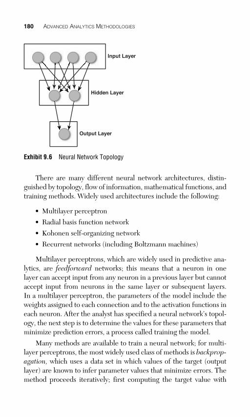
180 ADVANCED ANALYTICS METHODOLOGIES
There are many different neural network architectures, distin-guished by topology, flow of information, mathematical functions, and training methods. Widely used architectures include the following:
• Multilayer perceptron
• Radial basis function network
• Kohonen self-organizing network
• Recurrent networks (including Boltzmann machines)
Multilayer perceptrons, which are widely used in predictive ana-lytics, are feedforward networks; this means that a neuron in one layer can accept input from any neuron in a previous layer but cannot accept input from neurons in the same layer or subsequent layers. In a multilayer perceptron, the parameters of the model include the weights assigned to each connection and to the activation functions in each neuron. After the analyst has specified a neural network’s topol-ogy, the next step is to determine the values for these parameters that minimize prediction errors, a process called training the model.
Many methods are available to train a neural network; for multi-layer perceptrons, the most widely used class of methods is backprop-agation, which uses a data set in which values of the target (output layer) are known to infer parameter values that minimize errors. The method proceeds iteratively; first computing the target value with
Input Layer
Hidden Layer
Output Layer
Exhibit 9.6 Neural Network Topology

CHAPTER 9 • PREDICTIVE ANALYTICS TECHNIQUES 181
training data and then using information about prediction errors to adjust weights in the network.
Several different backpropagation algorithms exist; gradient descent and stochastic gradient descent are the most widely used. Gradient descent uses arbitrary starting values for the model param-eters and computes an error surface; it then seeks out a point on the error surface that minimizes prediction errors. Gradient descent eval-uates all cases in the training data set each time it iterates; stochastic gradient descent works with a random sample of cases from the train-ing data set. Consequently, stochastic gradient descent converges more quickly than gradient descent but may produce a less accurate model. The gradient descent algorithms can also train other types of models, including support vector machines and logistic regression.
Alternative algorithms for training a backpropagation neural net-work include the Broyden–Fletcher–Goldfarb–Shanno (BFGS) algo-rithm and its limited memory variant (L-BFGS) and the conjugate gradient algorithm. These algorithms can perform significantly better at minimizing prediction errors but tend to require more computing resources.
Radial basis function (RBF) networks have one or more hidden layers representing distance measures modeled with a Gaussian func-tion. Analysts train RBF networks with a maximum likelihood algo-rithm. Compared to multilayer perceptrons, RBF networks are less likely to confuse a local minimum in the error surface for the desired global minimum; however, they are also more prone to overfitting.
Kohonen self-organizing networks (self-organizing maps) are a technique for unsupervised learning with limited application in pre-dictive analytics. Refer to the appendix for a discussion of unsuper-vised learning with neural networks.
In a recurrent neural network (RNN), information flows in either direction among the layers; this contrasts with feedforward networks, where information flows in one direction only: from the input layer to the hidden layers to the output layer. The most important type of RNN is the restricted Boltzmann machine, an architecture used in deep learning (discussed in the following section).
The key strength of neural networks is their ability to model very complex nonlinear functions. Neural networks are also well suited to

182 ADVANCED ANALYTICS METHODOLOGIES
highly dimensional problems, where the number of potential predic-tors is very large.
The key weakness of neural networks is their tendency toward overlearning. A network learns to minimize prediction error on the training data, which is not the same thing as minimizing prediction error in a business application. As with other modeling techniques, analysts must test models produced with neural networks on an inde-pendent sample.
Analysts using the neural network technique must make a num-ber of choices about the network topology, transfer functions, activa-tion functions, and the training algorithm. Because there is very little theory to guide the choices, the analyst must rely on trial and error to find the best model. Consequently, neural networks tend to consume more analyst time to produce a useful model.
Leading commercial software packages for machine learning, including IBM SPSS Modeler, RapidMiner, SAS Enterprise Miner, and Statistica, support neural networks, as do in-database libraries such as dbLytix and Oracle Data Mining. Multiple packages in open source R support neural networks; in Python, the PyBrain package offers extensive capabilities.
Deep Learning
Deep learning is a class of model training techniques based on feature learning, or the capability to learn a concise set of “features” from complex unlabeled data. In practice, a deep neural network is a neural network with multiple hidden layers trained sequentially with unsupervised learning techniques.
Interest in deep learning stems from a number of notable recent successes in machine learning competitions:
• International Conference on Document Analysis and Recogni-tion (2009)
• IJCNN Traffic Sign Recognition Competition (2011, 2012)
• ISBI Segmentation of Neuronal Structures in Electron Micros-copy (2012)
• Merck Molecular Activity Challenge (2012)

CHAPTER 9 • PREDICTIVE ANALYTICS TECHNIQUES 183
The theory of deep learning dates to the 1980s; however, practical application lagged due to the computational complexity and resources needed. The increased availability and reduced cost of GPU devices and other platforms for high-performance computing has provided analysts with the computing power to experiment with deep learning techniques.
Deep neural networks are prone to overfitting due to the intro-duction of additional abstraction layers; analysts manage this tendency with regularization techniques. Models must be tested and validated to ensure they generalize to fresh cases.
Commercial software for deep learning is limited at present. Nei-ther SAS nor SPSS currently support the capability out of the box: PROC Neural in SAS Enterprise Miner 13.1 permits users to build neural networks with an unlimited number of hidden layers but lacks the ability to build Boltzmann machines, a necessary tool for deep learning. There are, however, a number of open source deep learn-ing libraries available in C, Java, and Python as well as a MATLAB Toolbox.
Support Vector Machines
Support vector machines (SVMs) evolved in the 1990s from pat-tern recognition research at Bell Labs. They work for either classifi-cation or regression, and are very useful when working with highly dimensional data—that is, when the number of potential predictors is very large.
The SVM algorithm depends on kernels, or transformations that map input data into a high-dimensional space. Kernel functions can be linear or nonlinear. After mapping the input data, the SVM algo-rithm constructs one or more hyperplanes that separate the data into homogeneous subgroups.
Given its robustness with highly dimensional data, SVM is well suited to applications in handwriting recognition, text categorization, or image tagging. In medical science, researchers successfully applied SVM to the detection of tumors in breast images and the classification of complex proteins.

184 ADVANCED ANALYTICS METHODOLOGIES
Commercial software packages that support SVM include Alpine Data Labs’ Alpine, IBM SPSS Modeler, Oracle Data Mining, SAS Enterprise Miner, and Statistica Data Miner. Open source options include Apache Spark MLLib, JKernalMachines, LIBSVM, and Vow-pal Wabbit. For R users, there are a number of packages, including kernlab, SVMMaj, gcdnet, obliqueRF, MVpower, svcR, and rasclass; for Python users, some SVM capabilities are included in scikit-learn and PyML.
Ensemble Learning
Ensemble Learning is a term we use to describe a number of techniques that generate many predictive models to produce a hybrid model with better predictive power than the individual models. There are a number of specific techniques in this category, which we describe below.
Overview
Ensemble learning techniques use multiple models to produce an aggregate model whose predictive power is better than individual models used alone. These techniques are computationally intensive and tend to require large amounts of data. The growth in available computing power makes ensemble learning, first introduced in the 1980s, accessible for mainstream users.
Boosting
Boosting is a class of iterative techniques that seeks to minimize overall errors by introducing additional models based on the errors from previous iterations. Among the many different boosting meth-ods, the most popular are ADABoost, Gradient Boosting, and Sto-chastic Gradient Boosting.
ADABoost
Introduced by Freund and Schapire in 1995, ADABoost (Adaptive Boosting) is one of the most popular methods for ensemble learning.

CHAPTER 9 • PREDICTIVE ANALYTICS TECHNIQUES 185
The ADABoost meta-algorithm operates iteratively, leveraging infor-mation about incorrectly classified cases to develop a strong aggregate model. With each pass, ADABoost tests possible classification rules and reweights them according to their ability to add to the overall predictive power of the model.
MathWorks offers a commercial implementation of ADABoost (part of the Statistics Toolbox). Many open source versions also are available, including implementations in C++, C#, Java, Python, and R.
Gradient Boosting
Jerome H. Friedman introduced gradient boosting and a variant, stochastic gradient boosting, in 1999. Like other boosting techniques, gradient boosting works with any base algorithm; however, it works best with relatively simple base models and is most widely used with decision tree learning. Gradient boosting works in a manner similar to ADABoost but uses a different measure to determine the cost of errors.
Stochastic gradient boosting combines gradient boosting with ran-dom subsampling (similar to bagging). In addition to improving model accuracy, this enhancement enables the analyst to predict model per-formance outside the training sample. Stochastic gradient boosting is similar to random forests because both methods train a large number of decision tree models. The difference between the two is that the stochastic gradient boosting algorithm uses information about classi-fication errors to guide the creation of incremental trees, whereas the random forests algorithm produces trees at random.
Salford Systems offers a commercial version of stochastic gradient boosting branded as TreeNet; StatSoft Data Miner supports a similar capability. Open source versions include implementations in C++ and Weka, as well as multiple packages in R.
Bootstrap Aggregation (Bagging)
Bagging is meta-algorithm proposed by Breiman in 1996. The bagging algorithm selects multiple subsamples from an original
186 ADVANCED ANALYTICS METHODOLOGIES
training data set, builds a model for each subsample, and then builds a solution through averaging (for regression) or through a voting pro-cedure (for classification).
The principal advantage of bagging is its ability to build more sta-ble models; its main disadvantage is its computational complexity and requirement for larger data sets. The growth of high-performance computing mitigates these disadvantages.
Random Forests
Random forests is an ensemble learning method for classification- and regression-based articles published by Ho, 5 Amit and Geman, 6 further developed by Breiman and Cutler, 7 and trademarked by Breiman and Cutler as “Random Forests.” The random forests algo-rithm combines bagging (random selection of subsets from the train-ing data) with a random selection of features, or predictors. The algorithm trains a large number of decision trees from randomly selected subsamples of the training data set and then outputs the class that is the mode of the class’s output by individual trees.
The principal advantage of random forests compared to other ensemble techniques is that its models generalize well outside the training sample. Moreover, random forests produces variable impor-tance measures that are useful for feature selection.
Salford Systems currently offers software based on the Breiman and Cutler article branded as “Random Forests” (under license from Breiman and Cutler). Open source versions are available in Apache Mahout, C#, Python, and R.
5 Ho, Tin Kam (1995), “Random Decision Forest,” Proceedings of the 3rd Inter-national Conference on Document Analysis and Recognition, Montreal, QC, http://cm.bell-labs.com/cm/cs/who/tkh/papers/odt.pdf .
6 Yali Amit and Donald Geman, “Shape Quantization and Recognition with Ran-domized Trees,” August 1996, http://www.cis.jhu.edu/publications/papers_in_database/GEMAN/shape.pdf .
7 Leo Breiman, “Random Forests,” October 2001, http://link.springer.com/article/10.1023%2FA%3A1010933404324 .
CHAPTER 9 • PREDICTIVE ANALYTICS TECHNIQUES 187
Automated Learning
Can you automate predictive modeling? The answer depends on the context. Consider the two variations on the following question, with more precise wording:
• Can you eliminate the need for expertise in predictive modeling—so that an “ordinary business user” can do it?
• Can you make expert analysts more productive by automating certain repetitive tasks?
The first form of the question—the search for “business user” analytics—is a common vision among software marketing profession-als and industry analysts; it assumes that expert analysts are the key bottleneck limiting enterprise adoption of predictive analytics. That premise is largely false, as is clear to anyone with a cursory under-standing of the overall process for predictive analytics in most orga-nizations. The answer is no; it is not possible to eliminate human expertise from predictive modeling, for the same reason that robotic surgery does not eliminate the need for cardiologists.
However, if you focus on the second form of the question and concentrate on how to make expert analysts more productive, the situation is much more promising. Many data preparation tasks are easy to automate; they include such tasks as detecting and eliminating zero-variance columns, treating missing values, and handling outliers. The most promising area for automation, however, is in model testing and assessment.
Optimizing a predictive model requires experimentation and tun-ing. For any given problem, there are many available modeling tech-niques, and for each technique, there are many ways to specify and parameterize a model. For the most part, trial and error is the only way to identify the best model for a given problem and data set. (The No Free Lunch Theorem 8 formalizes this concept.)
8 “No Free Lunch Theorems,” Retrieved June 25, 2014, from http://www.no-free-lunch.org/ .
188 ADVANCED ANALYTICS METHODOLOGIES
Because the best predictive model depends on the problem and the data, the analyst must search a very large set of feasible options to find the best model. In applied predictive analytics, however, the analyst’s time is strictly limited; a customer in the marketing services industry reports an SLA of 30 minutes or less for the analytics team to build a predictive model. Strict time constraints do not permit much time for experimentation.
Analysts tend to deal with this problem by settling for subop-timal models, arguing that models need only be “good enough,” or defending the use of one technique above all others. As clients grow more sophisticated, however, these tactics become ineffective. In high-stakes hard-money analytics—such as trading algorithms, cata-strophic risk analysis, and fraud detection—small improvements in model accuracy have a bottom-line impact, and clients demand the best possible predictions.
Automated modeling techniques are not new. Before Unica launched its successful suite of marketing automation software, the company’s primary business was analytic software, with a particular focus on neural networks. In 1995, Unica introduced Pattern Recog-nition Workbench (PRW), a software package that used automated trial and error to optimize a predictive model. Three years later, Unica partnered with Group 1 Software (now owned by Pitney Bowes) to market Model 1, a tool that automated model selection over four dif-ferent types of predictive models. Rebranded several times, the origi-nal PRW product remains as IBM PredictiveInsight, a set of wizards sold as part of IBM’s Enterprise Marketing Management suite.
Two other commercial attempts at automated predictive model-ing date from the late 1990s. The first, MarketSwitch, was less than successful. MarketSwitch developed and sold a solution for marketing offer optimization, which included an embedded “automated” predic-tive modeling capability (“developed by Russian rocket scientists”); in sales presentations, MarketSwitch promised customers its soft-ware would allow them to “fire their SAS programmers.” Experian acquired MarketSwitch in 2004, repositioned the product as a deci-sion engine, and replaced the “automated modeling” capability with outsourced analytic services.

CHAPTER 9 • PREDICTIVE ANALYTICS TECHNIQUES 189
KXEN, a company founded in France in 1998, built its analytics engine around an automated model selection technique called struc-tural risk minimization. The original product had a rudimentary user interface, depending instead on API calls from partner applications; more recently, KXEN repositioned itself as an easy-to-use solution for marketing analytics, which it attempted to sell directly to C-level executives. This effort was modestly successful, leading to the sale of the company in 2013 to SAP for an estimated $40 million.
In the past several years, the leading analytic software vendors (SAS and IBM SPSS) have added automated modeling features to their high-end products. In 2010, SAS introduced SAS Rapid Mod-eler, an add-in to SAS Enterprise Miner. Rapid Modeler is a set of macros implementing heuristics that handle tasks such as outlier identification, missing value treatment, variable selection, and model selection. The user specifies a data set and response measure; Rapid Modeler determines whether the response is continuous or categori-cal, and uses this information together with other diagnostics to test a range of modeling techniques. The user can control the scope of tech-niques to test by selecting basic, intermediate, or advanced methods.
IBM SPSS Modeler includes a set of automated data preparation features as well as Auto Classifier, Auto Cluster, and Auto Numeric nodes. The automated data preparation features perform such tasks as missing value imputation, outlier handling, date and time prepara-tion, basic value screening, binning, and variable recasting. The three modeling nodes enable the user to specify techniques to be included in the test plan, specify model selection rules, and set limits on model training.
All of the software discussed so far is commercially licensed. Two open source projects are worth noting: the caret package in open source R and the MLBase project. The caret package includes a suite of productivity tools designed to accelerate model specifica-tion and tuning for a wide range of techniques. The package includes preprocessing tools to support tasks such as dummy coding, detect-ing zero variance predictors, and identifying correlated predictors, as well as tools to support model training and tuning. The training func-tion in caret currently supports 149 different modeling techniques;

190 ADVANCED ANALYTICS METHODOLOGIES
it supports parameter optimization within a selected technique but does not optimize across techniques. To implement a test plan with multiple modeling techniques, the user must write an R script to run the required training tasks and capture the results.
MLBase, a joint project of the UC Berkeley AMPLab and the Brown University Data Management Research Group, is an ambi-tious effort to develop a scalable machine learning platform on Apache Spark. The ML Optimizer seeks to simplify machine learning problems for end users by automating the model selection task so that the user need only specify a response variable and set of predic-tors. The Optimizer project is still in active development, with Alpha release expected in 2014.
What have you learned from various attempts to implement auto-mated predictive modeling? Commercial startups like KXEN and MarketSwitch only marginally succeeded because they tried to over-sell the concept as a means to replace the analyst altogether. Most organizations understand that human judgment plays a key role in analytics, and they are not willing to entrust hard money analytics entirely to a black box.
What will the next generation of automated modeling platforms look like? Seven key features are critical for an automated modeling platform:
• Automated model-dependent data transformations
• Optimization across and within techniques
• Intelligent heuristics to limit the scope of the search
• Iterative bootstrapping to expedite search
• Massively parallel design
• Platform agnostic design
• Custom algorithms
Some methods require specific data transformations; neural nets, for example, typically work with standardized predictors, whereas Naïve Bayes and CHAID require all predictors to be categorical. The analyst should not have to perform these operations manually; instead, the modeling algorithm should build the transformations into

CHAPTER 9 • PREDICTIVE ANALYTICS TECHNIQUES 191
the test plan script and run them automatically; this ensures the maxi-mum number of possible techniques for any data set.
To find the best predictive model, you need to be able to search across techniques and tune parameters within techniques. Poten-tially, this can mean a massive number of model train-and-test cycles to run; you can use heuristics to limit the scope of techniques evalu-ated based on characteristics of the response measure and the pre-dictors. (For example, a categorical response rules out a number of techniques, and a continuous response measure rules out a differ-ent set of techniques.) Instead of a brute force search for the best technique and parameterization, a “bootstrapping” approach can use information from early iterations to specify subsequent tests.
Even with heuristics and bootstrapping, a comprehensive experi-mental design may require thousands of model train-and-test cycles; this is a natural application for massively parallel computing. More-over, the highly variable workload inherent in the development phase of predictive analytics is a natural application for cloud (a point that deserves yet another blog post of its own). The next generation of automated predictive modeling will be in the cloud from its inception.
Ideally, the model automation wrapper should be agnostic to specific implementations of machine learning techniques; the user should be able to optimize across software brands and versions. Real-istically, commercial vendors such as SAS and IBM will never permit their software to run under an optimizer that they do not own; hence, as a practical matter, you should assume that the next generation pre-dictive modeling platform will work with open source machine learn-ing libraries, such as R or Python.
You cannot eliminate the need for human expertise from predic-tive modeling, but you can build tools that enable analysts to build better models.
Summary
In this chapter, we surveyed key techniques for predictive ana-lytics. Some techniques, such as linear regression, are mature, well understood, widely used, and broadly available in stable software

192 ADVANCED ANALYTICS METHODOLOGIES
tools. Other methods, such as deep learning, are quite new. Scien-tists still seek to understand the limits of such techniques; software implementations are rare, and they are not yet widely used in analyti-cal applications. A third category of techniques, including automated learning, is in active development as we write this book.
As we noted at the beginning of this chapter, hundreds of pre-dictive modeling techniques are in use, and scientists add new tech-niques every day. As with any technology, practitioners make small changes to address specific problems—produce more accurate mod-els with specific types of data, run faster, work efficiently with more predictors, and so forth.
The business stakeholder need not understand every detail of the techniques used by analysts to build predictive models; instead, the stakeholder should focus on two key principles. First, in most cases, it is impossible to know in advance what technique will produce the most accurate predictions for a particular problem; the only way to discover this is to experiment with a broad spectrum of techniques. (The stakeholder should view with suspicion claims that any one method is always the best method.)
Second, the ultimate test of any predictive model is how well it predicts when placed in production. The theoretical merits and demerits of various techniques are interesting to academics; in actual applications, however, predictive power and performance are the sole measure of a model.

This page intentionally left blank

Index
A a priori segmentation, 158 Abbott, Dean, 21
case study, 37 - 42 , 51 accuracy of classification, 137 ACID (Atomic, Consistent, Isolation,
Durability), 244 ad hoc analysis, 9 , 89 - 91 ADABoost (Adaptive Boosting), 184 Adams, John, 262 agent-based modeling, 43 aggregate functions, 205 Air Liquide case study, 36 - 37 , 51 Akaike information criterion (AIC), 140 algorithms in analytics roadmap, 23 Alpine, 216 - 217 , 227 , 232 Alteryx, 217 ambition factors of data scientists,
266 - 269 analysis data set
building, 128 - 133 assembling data, 129 evaluating data, 129 - 130 investigating outliers, 130 - 131 missing data, 133 table operations, 132 transforming data, 131 - 132
partitioning, 135 - 136 analytic applications in customer-facing
analytics, 100 - 101 analytic libraries (SQL), 247 analytic personas, 11 analytic solutions
brainstorming, 65 - 70 describing, 70 - 74 establishing roadmap, 84-86 prioritizing, 74 - 76 scoring, 76 - 83
analytic talent. See data scientists
313
analytics business culture and, 258 - 259
change, 261 - 262 curiosity, 259 - 260 evidence, 262 experimentation, 261 problem solving, 260
business user tools, 209 Alpine, 216 - 217 Alteryx, 217 BI (business intelligence)
techniques, 209 - 216 IBM SPSS Modeler, 217 - 218 RapidMiner, 218 SAS Enterprise Guide, 218 SAS Enterprise Miner, 219 Statistica, 219 - 220 usage by user personas, 220
complexities of deployment, 257 customer-facing analytics, 67 , 99 - 101
analytic applications, 100 - 101 consumer analytics, 101 prediction services, 100
descriptive analytics, 67 distributed analytics, 224 - 228 , 238 - 241 managerial analytics, 66 , 93 - 95 operational analytics, 66 , 95 - 98 possible uses, 25 - 26 predictive analytics, 67 - 68
analysis data set, building, 128 - 133
anomaly detection, 152 - 154 architectures, 228 - 243 automated learning, 187 - 191 Bayesian belief networks,
155 - 156 , 177 - 178 Big Data, impact of, 150 - 151 business needs, defining, 122 - 128 capabilities, 214 clustering techniques, 158 - 159 decision tree learning, 174 - 177 deep learning, 182 - 183

314 INDEX
deployability, 98 dimension reduction, 160 - 161 distributed computing and,
224 - 228 ensemble learning, 184 - 186 generalized additive model
(GAM), 168 generalized linear models,
167 - 168 goals, 119 - 120 graph and network analysis, 154 linear models, 162 - 163 linear regression, 164 - 166 logistic regression, 169 - 170 methodologies, 120 - 121 neural networks, 179 - 182 ,
297 - 310 predictive model, building,
133 - 141 predictive model, deploying,
141 - 146 regularization, 172 - 173 statistics versus machine
learning, 149 stepwise regression, 171 - 172 supervised versus unsupervised
learning techniques, 152 support vector machines (SVMs),
183 - 184 survival analysis, 173 - 174 text mining, 156 - 157 use case, 106 - 109
prescriptive analytics, 68 principles of
accelerate learning and execution, 7 - 8
building human factors, 11 consumerization, 12 deliver business value and
impact, 3 - 4 differentiation, 8 - 9 embedded analytics, 9 establish lean architecture, 9 - 11 focus on last mile, 4 - 6 leverage Kaizen, 6 - 7 list of, 2
programming languages, 199 Python, 206 - 209 R Project, 199 - 203 SAS programming language,
203 - 204 SQL (Structured Query
Language), 204 - 206 requirements, 213 scientific analytics, 67 , 98 - 99 simulation analytics, 68
strategic analytics, 66 , 88 - 93 ad hoc analysis, 89 - 91 business simulation, 92 - 93 econometric forecasting, 91 - 92 market segmentation, 91
success factors, 194 - 195 teams
analytics program office, 291 Center of Excellence (COE),
288 - 289 centralized versus decentralized,
283 - 287 chief data officer versus chief
analytics officer, 289 - 291 lab teams, 291 organizing, 283
types of, 66 - 67 , 88 , 294 unique analytics roadmap, 19 - 20
algorithms, 23 analytic solutions, brainstorming,
65 - 70 analytic solutions, describing,
70 - 74 analytic solutions, establishing
roadmap, 84 analytic solutions, prioritizing,
74 - 76 analytic solutions, scoring, 76 - 83 approach, 21 - 22 building, 295 business area, 20 - 21 case study, 51 - 59 data sources, 21 deploying, 293 - 294 embedded analytics, 23 evaluating, 86 importance of, 61 key business objectives
identification, 61 - 62 precision, 22 rough-cut project estimates,
creating, 83 speed, 23 updating, 86 value chain definition, 62 - 65
use cases discovery, 111 - 116 explanation, 109 - 110 forecasting, 110 - 111 optimization, 117 overview, 103 - 104 prediction, 106 - 109 simulation, 116 - 117
user personas analytics consumers, 198 - 199 business analysts, 197 - 198
INDEX 315
data scientists, 197 list of, 195 power analysts, 195 - 196 tools used by, 220
analytics consumers, 198 - 199 , 220 analytics generalists, 274 - 275 analytics managers, 272 - 274 analytics program office, 291 analytics programmers, 271 - 272 “Analytics: The Widening Divide” (MIT
Sloan School of Management), 26 - 27 anomaly detection, 152 - 154 anomaly detection in Discovery use
case, 114 - 115 ANSI SQL standard, 205 - 206 ant systems, 36 - 37 Apache Cassandra, 241 Apache Giraph, 236 Apache Hive, 236 , 251 Apache Mahout, 227 , 236 , 240 Apache Spark, 237 - 241 app stores, 12 appliances, 248 applications for unsupervised learning
techniques, 310 applied decision systems, 97 approach in analytics roadmap, 21 - 22 approving predictive model, 142 architectures
lean analytics architectures, 9 - 11 neural network architectures,
180 - 181 , 298 Kohonen self-organizing
networks, 299 - 304 neocognitron networks, 307 - 309 neural gas networks, 305 - 307
predictive analytics architectures, 228 - 243
distributed analytics with Apache Spark, 238 - 241
freestanding analytics, 229 - 231 in cloud, 241 - 243 in-Hadoop analytics, 235 - 238 partially integrated analytics,
231 - 233 in-database analytics, 233 - 235 artificial neural networks. See neural
networks asset management in predictive
analytics, 145 - 146 association in Discovery use case,
113 - 114 At Home in the Universe: The Search
for Laws of Self-Organization and Complexity (Kauffman), 42
attracting data scientists, 264 - 265 , 280 - 281
attribution analysis, 95 automation, 16 - 18
automated learning, 187 - 191 in stepwise regression, 171
B backpropagation, 180 - 181 backtesting, 4 , 31 backward selection in stepwise
regression, 171 backward validation, 4 bagging, 185 - 186 batch deployment in predictive
analytics, 127 - 128 , 144 batch SQL, 246 Bayesian belief networks, 155 - 156 ,
177 - 178 Bayesian information criterion
(BIC), 140 Beiersdorf case study, 35 - 36 , 51 belief networks, 155 - 156 , 177 - 178 BFGS
(Broyden-Fletcher-Goldfarb-Shanno) algorithm, 181
BI (business intelligence) techniques, 209 - 210
history of, 210 - 216 bidirectional stepwise in stepwise
regression, 171 Big Data, impact of, 150 - 151 binomial classification, 169 biological origin of Kohonen networks,
300 - 301 BiosGroup, 42 BMW case study, 44 - 46 , 51 boosting, 184 bootstrap aggregation (bagging),
185 - 186 brainstorming analytic solutions, 65 - 70 bring your own data (BYOD), 12 bring your own models (BYOM), 12 bring your own tools (BYOT), 12 Broyden-Fletcher-Goldfarb-Shanno
(BFGS) algorithm, 181 budget in analytics roadmap, 78 built-in functions (SQL), 247 business analysts, 197 - 198 , 220 business and technology history, 16 - 18 business area in analytics roadmap,
20 - 21

316 INDEX
business culture, 258 - 259 change, 261 - 262 curiosity, 259 - 260 evidence, 262 experimentation, 261 problem solving, 260
business intelligence (BI) techniques, 209 - 210
history of, 210 - 216 business needs, defining, 122 - 128 business objectives, identifying, 61 - 62 business simulation, 92 - 93 business user tools, 209
Alpine, 216 - 217 Alteryx, 217 BI (business intelligence) techniques,
209 - 210 history of, 210 - 216
IBM SPSS Modeler, 217 - 218 RapidMiner, 218 SAS Enterprise Guide, 218 SAS Enterprise Miner, 219 Statistica, 219 - 220 usage by user personas, 220
business value, measuring, 3 - 4 BYOD (bring your own data), 12 BYOM (bring your own models), 12 BYOT (bring your own tools), 12
C C4.5, 177 C5.0, 177 call center example (workforce
performance), 33 - 35 caret package (open source R), 189 - 190 CART (Classification and Regression
Trees), 176 - 177 case studies, 52-59
Air Liquide, 36 - 37 , 51 Beiersdorf, 35 - 36 , 51 BMW, 44 - 46 , 51 DataSong, 28 - 32 , 51 Dean Abbott, 37 - 42 , 51 Express Scripts, 49 - 50 Gartner Research, 49 - 50 Infinity Insurance, 50 McDonald’s, 50 Obama campaign, 46 - 47 , 51 P&G (Procter and Gamble), 42 - 44 , 51 Southwest Airlines, 47 - 48 , 51 Talent Analytics, 32 - 35 , 51 Vestas (wind turbines), 48 - 49 , 51
censoring, 173 Center of Excellence (COE), 288 - 289
centralized teams, decentralized versus, 283 - 287
CHAID (Chi-Square Automatic Interaction Detection), 175 - 176
Champy, James, 16 - 17 change in business culture, 261 - 262 Charlotte Software Systems, 37 chief analytics officer, chief data officer
versus, 289 - 291 chief data officer, chief analytics officer
versus, 289 - 291 Chi-Square Automatic Interaction
Detection (CHAID), 175 - 176 classification
accuracy, 137 with logistic regression, 169 - 170 regression versus, 125 sensitivity, 138
Classification and Regression Trees (CART), 176 - 177
cloud-based analytics, 241 - 243 Cloudera, 240 Cloudera Impala, 251 clustering techniques, 112 - 113 , 158 - 159 Clustrix, 253 Codd, Edgar, 244 COE (Center of Excellence), 288 - 289 Competitive Advantage: Creating and
Sustaining Superior Performance (Porter), 62
competitive differentiation, history of, 16 - 18
competitive learning, 298 Competitive Strategy: Techniques for
Analyzing Industries and Competitors (Porter), 19
complexity science (Southwest Airlines case study), 47 - 48
conjugate gradient algorithm, 181 connectors (Hadoop), 250 consumer analytics in customer-facing
analytics, 101 consumerization, 12 continuous improvement. See Kaizen core activities, 62 cost of errors, 125 - 126 Cox’s proportional hazards (CPH)
model, 174 credit risk analysis, 110 crowdsourcing, 12 culture. See business culture curiosity in business culture, 259 - 260 customer interaction (DataSong case
study), 28 - 32 customer segmentation, 158
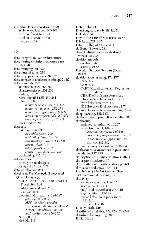
INDEX 317
customer-facing analytics, 67 , 99 - 101 analytic applications, 100 - 101 consumer analytics, 101 prediction services, 100 use cases, 105
D data integration. See architectures data mining (Infinity Insurance case
study), 50 data munging, 39 , 132 data parallel tasks, 226 data prep professionals, 269 - 271 data science in analytics roadmap, 21 - 22 data scientists, 197
ambition factors, 266 - 269 characteristics of, 262 - 269 finding, 279 - 280 recruiting, 264 - 265 , 280 - 281 roles of, 266
analytics generalists, 274 - 275 analytics managers, 272 - 274 analytics programmers, 271 - 272 data prep professionals, 269 - 271 sample job structure, 275 - 279
tools used by, 220 data sets
building, 128 - 133 assembling data, 129 evaluating data, 129 - 130 investigating outliers, 130 - 131 missing data, 133 table operations, 132 transforming data, 131 - 132
partitioning, 135 - 136 data sources
in analytics roadmap, 21 for Apache Spark, 239
data warehouses, 244 databases . See also SQL (Structured
Query Language) ACID (Atomic, Consistent, Isolation,
Durability), 244 in-database analytics, 229 ,
233 - 235 , 244 modern SQL platforms, 244 - 247
future of, 255 - 256 MPP (massively parallel
processing) databases, 247 - 250 NewSQL databases, 252 - 254 SQL-on-Hadoop, 250 - 252
NewSQL, 245 NoSQL, 245
Databricks, 241 DataSong case study, 28 - 32 , 51 Datastax, 241 Day-in-the-Life-of-Scenarios, 78 - 83 DB Lytix, 227 , 235 DB2 Intelligent Miner, 234 de Bono, Edward, 261 decentralized teams, centralized
versus, 283 - 287 decision models
creating, 74 - 76 scoring, 76 - 83
Decision Support Systems (DSS), 211 - 213
decision tree learning, 174 - 177 C4.5, 177 C5.0, 177 CART (Classification and Regression
Trees), 176 - 177 CHAID (Chi-Square Automatic
Interaction Detection), 175 - 176 hybrid decision trees, 177 ID3 (Iterative Dichotomiser), 177
decision trees in decision analysis, 39 - 42 deep learning, 182 - 183 deployability in predictive analytics, 98 deploying
analytics, complexities of, 257 predictive model, 141 - 146
asset management, 145 - 146 measuring performance, 144 - 145 reviewing and approving, 142 scoring, 142 - 144
unique analytics roadmap, 293 - 294 deployment environment in predictive
analytics, 127 - 128 descriptions of analytic solutions, 70 - 74 descriptive analytics, 67 differentiation of analytic strategy, 8 - 9 dimension reduction, 160 - 161 Discipline of Market Leaders, The
(Treacy and Wiersema), 17 discovery
anomaly detection, 114 - 115 association, 113 - 114 graph and network analysis, 116 segmentation, 112 - 113 text and document processing,
111 - 112 use case, 111 - 116
Disney, Walt, 259 distributed analytics, 224 - 228 , 238 - 241 distributed computing, 225 Divis, 36 , 46
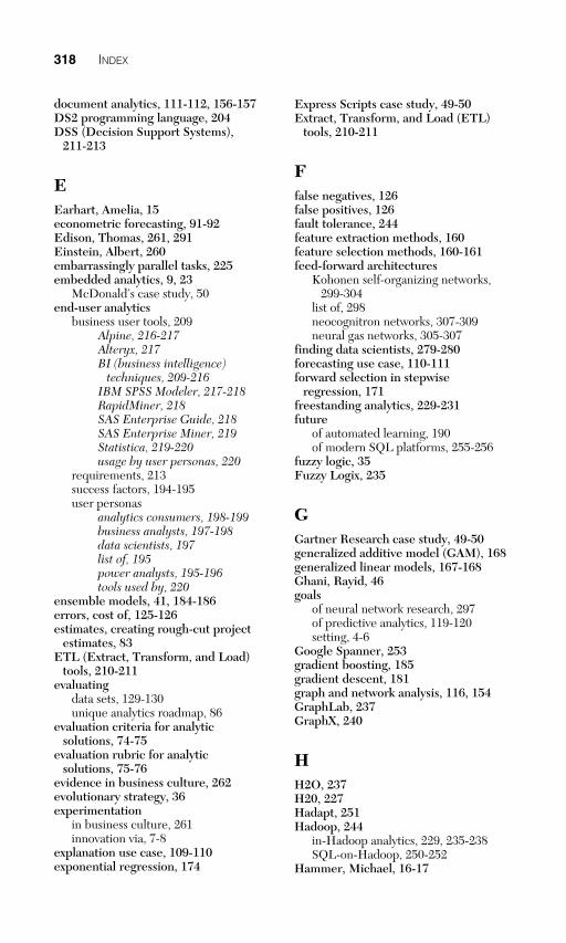
318 INDEX
document analytics, 111 - 112 , 156 - 157 DS2 programming language, 204 DSS (Decision Support Systems),
211 - 213
E Earhart, Amelia, 15 econometric forecasting, 91 - 92 Edison, Thomas, 261 , 291 Einstein, Albert, 260 embarrassingly parallel tasks, 225 embedded analytics, 9 , 23
McDonald’s case study, 50 end-user analytics
business user tools, 209 Alpine, 216 - 217 Alteryx, 217 BI (business intelligence)
techniques, 209 - 216 IBM SPSS Modeler, 217 - 218 RapidMiner, 218 SAS Enterprise Guide, 218 SAS Enterprise Miner, 219 Statistica, 219 - 220 usage by user personas, 220
requirements, 213 success factors, 194 - 195 user personas
analytics consumers, 198 - 199 business analysts, 197 - 198 data scientists, 197 list of, 195 power analysts, 195 - 196 tools used by, 220
ensemble models, 41 , 184 - 186 errors, cost of, 125 - 126 estimates, creating rough-cut project
estimates, 83 ETL (Extract, Transform, and Load)
tools, 210 - 211 evaluating
data sets, 129 - 130 unique analytics roadmap, 86
evaluation criteria for analytic solutions, 74 - 75
evaluation rubric for analytic solutions, 75 - 76
evidence in business culture, 262 evolutionary strategy, 36 experimentation
in business culture, 261 innovation via, 7 - 8
explanation use case, 109 - 110 exponential regression, 174
Express Scripts case study, 49 - 50 Extract, Transform, and Load (ETL)
tools, 210 - 211
F false negatives, 126 false positives, 126 fault tolerance, 244 feature extraction methods, 160 feature selection methods, 160 - 161 feed-forward architectures
Kohonen self-organizing networks, 299 - 304
list of, 298 neocognitron networks, 307 - 309 neural gas networks, 305 - 307
finding data scientists, 279 - 280 forecasting use case, 110 - 111 forward selection in stepwise
regression, 171 freestanding analytics, 229 - 231 future
of automated learning, 190 of modern SQL platforms, 255 - 256
fuzzy logic, 35 Fuzzy Logix, 235
G Gartner Research case study, 49 - 50 generalized additive model (GAM), 168 generalized linear models, 167 - 168 Ghani, Rayid, 46 goals
of neural network research, 297 of predictive analytics, 119 - 120 setting, 4 - 6
Google Spanner, 253 gradient boosting, 185 gradient descent, 181 graph and network analysis, 116 , 154 GraphLab, 237 GraphX, 240
H H2O, 237 H20, 227 Hadapt, 251 Hadoop, 244
in-Hadoop analytics, 229 , 235 - 238 SQL-on-Hadoop, 250 - 252
Hammer, Michael, 16 - 17

INDEX 319
heroes, 15 - 16 , 18 history
of automated learning, 188 - 189 of BI (business intelligence)
techniques, 210 - 216 of business and technology, 16 - 18 of SQL (Structured Query Language),
243 - 244 Hortonworks Stinger, 251 HP Vertica, 249 HTAP (Hybrid Transaction and
Analytical Processing), 255 human role in analytics, 11 hybrid decision trees, 177 hybrid teams, 285 Hybrid Transaction and Analytical
Processing (HTAP), 255
I IBM Netezza Analytics, 234 IBM PureData, 234 , 249 IBM SPSS Analytic Server, 227 IBM SPSS Modeler, 189 , 217 - 218 , 232 ID3 (Iterative Dichotomiser), 177 in-database analytics, 229 , 233 - 235 , 244 in-Hadoop analytics, 229 , 235 - 238 Infinity Insurance case study, 50 Infonomics (Laney), 49 innovation via experimentation, 7 - 8 integration of data. See architectures interactive design (BMW case study),
44 - 46 interactive SQL, 246 inventory supply chain, P&G (Procter
and Gamble) case study, 42 - 44 Iterative Dichotomiser (ID3), 177
K Kaizen, 6 - 7 Kauffman, Stuart, 42 Keller, Helen, 15 k-means clustering, 159 key business objectives, identifying,
61 - 62 Kohonen self-organizing networks,
181 , 298 - 304 KXEN, 188 - 189
L lab teams, 291 Laney, Doug, 49 LASSO regularization, 173 lean analytics architectures, 9 - 11 linear models
generalized linear models, 167 - 168 standard linear models, 162 - 163
linear parallel tasks, 225 linear regression
generalized additive model (GAM), 168
parametric technique, 164 - 166 log-normal regression, 174 logistic regression, 169 - 170
M machine learning, statistics versus, 149 MADLib, 227 managerial analytics, 66 , 93 - 95 , 105 MapReduce, 236 - 237 market segmentation, 91 , 158 marketing mix modeling, 28 MarketSwitch, 188 Markov blankets, 178 massively parallel processing (MPP)
databases, 247 - 250 , 255 maximum likelihood algorithm, 170 McDonald’s case study, 50 measuring
business value, 3 - 4 performance of predictive model,
136 - 140 , 144 - 145 MemSQL, 253 methodologies for predictive analytics,
120 - 121 analysis data set, building, 128 - 133 business needs, defining, 122 - 128 predictive model
building, 133 - 141 deploying, 141 - 146
missing data, 133 ML Optimizer, 190 MLBase, 190 MLLib, 227 , 240 Model Building subcase (Prediction use
case), 106 model repository management in
predictive analytics, 145 - 146 Model Scoring subcase (Prediction use
case), 106
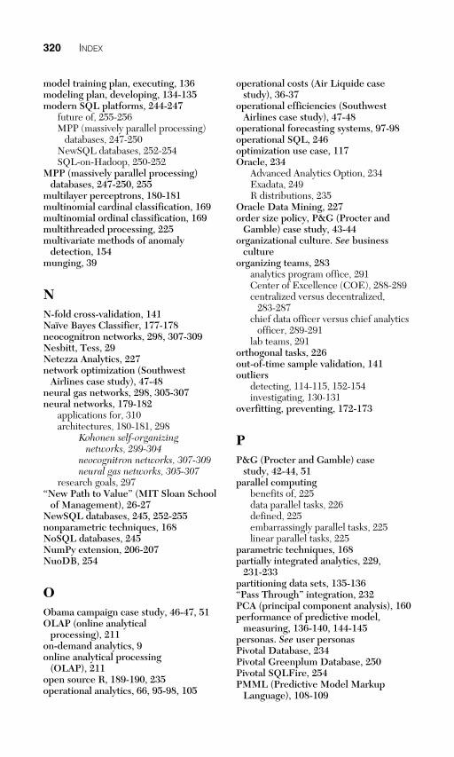
320 INDEX
model training plan, executing, 136 modeling plan, developing, 134 - 135 modern SQL platforms, 244 - 247
future of, 255 - 256 MPP (massively parallel processing)
databases, 247 - 250 NewSQL databases, 252 - 254 SQL-on-Hadoop, 250 - 252
MPP (massively parallel processing) databases, 247 - 250 , 255
multilayer perceptrons, 180 - 181 multinomial cardinal classification, 169 multinomial ordinal classification, 169 multithreaded processing, 225 multivariate methods of anomaly
detection, 154 munging, 39
N N-fold cross-validation, 141 Naïve Bayes Classifier, 177 - 178 neocognitron networks, 298 , 307 - 309 Nesbitt, Tess, 29 Netezza Analytics, 227 network optimization (Southwest
Airlines case study), 47 - 48 neural gas networks, 298 , 305 - 307 neural networks, 179 - 182
applications for, 310 architectures, 180 - 181 , 298
Kohonen self-organizing networks, 299 - 304
neocognitron networks, 307 - 309 neural gas networks, 305 - 307
research goals, 297 “New Path to Value” (MIT Sloan School
of Management), 26 - 27 NewSQL databases, 245 , 252 - 255 nonparametric techniques, 168 NoSQL databases, 245 NumPy extension, 206 - 207 NuoDB, 254
O Obama campaign case study, 46 - 47 , 51 OLAP (online analytical
processing), 211 on-demand analytics, 9 online analytical processing
(OLAP), 211 open source R, 189 - 190 , 235 operational analytics, 66 , 95 - 98 , 105
operational costs (Air Liquide case study), 36 - 37
operational efficiencies (Southwest Airlines case study), 47 - 48
operational forecasting systems, 97 - 98 operational SQL, 246 optimization use case, 117 Oracle, 234
Advanced Analytics Option, 234 Exadata, 249 R distributions, 235
Oracle Data Mining, 227 order size policy, P&G (Procter and
Gamble) case study, 43 - 44 organizational culture. See business
culture organizing teams, 283
analytics program office, 291 Center of Excellence (COE), 288 - 289 centralized versus decentralized,
283 - 287 chief data officer versus chief analytics
officer, 289 - 291 lab teams, 291
orthogonal tasks, 226 out-of-time sample validation, 141 outliers
detecting, 114 - 115 , 152 - 154 investigating, 130 - 131
overfitting, preventing, 172 - 173
P P&G (Procter and Gamble) case
study, 42 - 44 , 51 parallel computing
benefits of, 225 data parallel tasks, 226 defined, 225 embarrassingly parallel tasks, 225 linear parallel tasks, 225
parametric techniques, 168 partially integrated analytics, 229 ,
231 - 233 partitioning data sets, 135 - 136 “Pass Through” integration, 232 PCA (principal component analysis), 160 performance of predictive model,
measuring, 136 - 140 , 144 - 145 personas. See user personas Pivotal Database, 234 Pivotal Greenplum Database, 250 Pivotal SQLFire, 254 PMML (Predictive Model Markup
Language), 108 - 109
INDEX 321
POCs (Proof-of-Concepts), 6 Porter, Michael, 19 , 62 power analysts, 195 - 196 , 220 precision in analytics roadmap, 22 prediction services in customer-facing
analytics, 100 prediction windows, determining, 127 predictive analytics, 67 - 68
architectures, 228 - 243 distributed analytics with Apache
Spark, 238 - 241 freestanding analytics, 229 - 231 in cloud, 241 - 243 in-database analytics, 233 - 235 in-Hadoop analytics, 235 - 238 partially integrated analytics,
231 - 233 capabilities, 214 deployability, 98 distributed computing and, 224 - 228 goals, 119 - 120 methodologies, 120 - 121
analysis data set, building, 128 - 133
business needs, defining, 122 - 128 predictive model, building,
133 - 141 predictive model, deploying,
141 - 146 techniques
anomaly detection, 152 - 154 automated learning, 187 - 191 Bayesian belief networks,
155 - 156 , 177 - 178 Big Data, impact of, 150 - 151 clustering techniques, 158 - 159 decision tree learning, 174 - 177 deep learning, 182 - 183 dimension reduction, 160 - 161 ensemble learning, 184 - 186 generalized additive model
(GAM), 168 generalized linear models,
167 - 168 graph and network analysis, 154 linear models, 162 - 163 linear regression, 164 - 166 logistic regression, 169 - 170 neural networks, 179 - 182 ,
297 - 310 regularization, 172 - 173 statistics versus machine
learning, 149 stepwise regression, 171 - 172 supervised versus unsupervised
learning techniques, 152
support vector machines (SVMs), 183 - 184
survival analysis, 173 - 174 text mining, 156 - 157
use case, 106 - 109 predictive model
building, 133 - 141 measuring performance, 136 - 140 model training plan, 136 modeling plan, developing,
134 - 135 partitioning data set, 135 - 136
deploying, 141 - 146 asset management, 145 - 146 measuring performance, 144 - 145 reviewing and approving, 142 scoring, 142 - 144
validating, 140 - 141 Predictive Model Markup Language
(PMML), 108 - 109 predictor variables in modeling plan
development, 134 - 135 prescriptive analytics, 68 principal component analysis (PCA), 160 principles of analytics
accelerate learning and execution, 7 - 8 building human factors, 11 consumerization, 12 deliver business value and impact, 3 - 4 differentiation, 8 - 9 embedded analytics, 9 establish lean architecture, 9 - 11 focus on last mile, 4 - 6 leverage Kaizen, 6 - 7 list of, 2
prioritizing analytic solutions, 74 - 76 private knowledge, 98 probing questions in value chain
brainstorming, 68 - 69 problem solving in business culture, 260 Procter and Gamble (P&G) case study,
42 - 44 , 51 product development cycle (BMW case
study), 44 - 46 product innovation (Beiersdorf case
study), 35 - 36 programming languages for
analytics, 199 Python, 206 - 209 R Project, 199 - 203 SAS programming language, 203 - 204 SQL (Structured Query Language),
204 - 206 Proof-of-Concepts (POCs), 6 public knowledge, 98

322 INDEX
“Push Down” integration, 232 Python, 206 - 209
R R Project, 199 - 203
open source R, 189 - 190 , 235 Oracle R distributions, 235
radial basis function (RBF) networks, 181
random forests, 186 RapidMiner, 218 RDDs (Resilient Distributed
Datasets), 239 real-time SQL, 246 Receiver Operating Characteristic
(ROC) curve, 139 recruiting data scientists, 264 - 265 ,
280 - 281 recurrent neural networks (RNN), 181 Reengineering the Corporation
(Hammer and Champy), 16 - 17 regression
classification versus, 125 exponential regression, 174 linear regression
generalized additive model (GAM), 168
parametric technique, 164 - 166 log-normal regression, 174
logistic regression, 169 - 170 stepwise regression, 171 - 172
regularization, 172 - 173 reinforcement learning, 298 Resilient Distributed Datasets
(RDDs), 239 response measures, defining, 123 - 125 response-attribution analysis, 109 reviewing predictive model, 142 Revolution R Enterprise, 227 ridge regularization, 173 risk assessment, 93 RMSE (root mean square error), 140 RNN (recurrent neural networks), 181 roadmap. See unique analytics roadmap Roberts, Greta, 32 , 263 ROC (Receiver Operating
Characteristic) curve, 139 root mean square error (RMSE), 140 rough-cut project estimates, creating, 83 Roumeliotis, George, 286 , 290
S sampling, 150 SAP HANA, 254 SAS Enterprise Guide, 218 SAS Enterprise Miner, 219 , 233 SAS High Performance Analytics, 227 SAS programming language,
203 - 204 , 232 SAS Rapid Modeler, 189 SAS Scoring Accelerator, 233 scalar functions, 205 scientific analytics, 67 , 98 - 99 , 105 scikit-learn package, 207 SciPy extension, 206 - 207 scoring
analytic solutions, 76 - 83 partially integrated analytics, 231 - 233 prediction versus, 106 - 109 predictive model, 142 - 144
segmentation in Discovery use case, 112 - 113 market segmentation in strategic
analytics, 91 types of, 158 - 159
self-organizing feature map. See Kohonen self-organizing networks
sensitivity of classification, 138 sentiment analysis, 112 service calls (Dean Abbott case
study), 37 - 42 simulation analytics, 68 , 116 - 117 Six Thinking Hats (de Bono), 261 Skytree Server, 227 Smarter Remarketer case study, 37 - 42 Socrates, 261 software. See architectures; business
user tools; modern SQL platforms Southwest Airlines case study, 47 - 48 , 51 Spark. See Apache Spark Spark Streaming, 240 speed in analytics roadmap, 23 Splice Machine, 252 split-sample validation, 141 spreadsheet-based DSS (Decision
Support Systems), 211 - 213 SQL (Structured Query Language),
204 - 206 history of, 243 - 244 modern SQL platforms, 244 - 247
future of, 255 - 256 MPP (massively parallel
processing) databases, 247 - 250 NewSQL databases, 252 - 254 SQL-on-Hadoop, 250 - 252

INDEX 323
SQL-on-Hadoop, 250 - 252 , 255 standard linear models, 162 - 163 State University of New York (SUNY) at
Buffalo, 99 Statistica, 219 - 220 statistics, machine learning versus, 149 stepwise regression, 171 - 172 stochastic gradient boosting, 185 stochastic gradient descent, 181 strategic analytics, 66 , 88 - 93
ad hoc analysis, 89 - 91 business simulation, 92 - 93 econometric forecasting, 91 - 92 market segmentation, 91 use cases, 105
strategic segmentation, 158 streaming SQL, 247 Structured Query Language (SQL). See
SQL (Structured Query Language) SUNY (State University of New York) at
Buffalo, 99 supervised learning techniques
in neural networks, 297 unsupervised learning techniques
versus, 152 supply chain, P&G (Procter and
Gamble) case study, 42 - 44 support activities, 62 support vector machines (SVMs),
183 - 184 survival analysis, 29 , 173 - 174
T table operations, building data sets, 132 talent. See data scientists; teams Talent Analytics case study, 32 - 35 , 51 targeting (Obama campaign case
study), 46 - 47 targeting and routing systems, 97 teams, organizing, 283
analytics program office, 291 Center of Excellence (COE), 288 - 289 centralized versus decentralized,
283 - 287 chief data officer versus chief analytics
officer, 289 - 291 lab teams, 291
techniques for predictive analytics anomaly detection, 152 - 154 automated learning, 187 - 191 Bayesian belief networks, 155 - 156 ,
177 - 178 Big Data, impact of, 150 - 151 clustering techniques, 158 - 159
decision tree learning, 174 - 177 deep learning, 182 - 183 dimension reduction, 160 - 161 ensemble learning, 184 - 186 graph and network analysis, 154 linear models
generalized linear models, 167 - 168
standard linear models, 162 - 163 linear regression
generalized additive model (GAM), 168
parametric technique, 164 - 166 logistic regression, 169 - 170 neural networks, 179 - 182 , 297 - 310 regularization, 172 - 173 statistics versus machine learning, 149 stepwise regression, 171 - 172 supervised versus unsupervised
learning techniques, 152 support vector machines (SVMs),
183 - 184 survival analysis, 173 - 174 text mining, 156 - 157
technology and business history, 16 - 18 Teradata, 234- 235 , 250 Teradata SQL-H, 252 text analytics, 38 , 111 - 112 text mining, 112 , 156 - 157 time series analysis, 110 - 111 time-to-event measures, 173 - 174 timeline in analytics roadmap, 78 tools. See architectures; business user
tools; modern SQL platforms topology
of Kohonen networks, 300 - 301 of neocognitron networks, 308 of neural gas networks, 305
transactional deployment in predictive analytics, 127 - 128 , 144
transforming data, 131 - 132 TransLattice, 254 Treacy, Michael, 17 tree-building. See decision tree learning turnout model, 46
U UDFs (user-defined functions), 247 Unica, 188 unique analytics roadmap, 19 - 20
building analytic solutions, brainstorming,
65 - 70 analytic solutions, describing,
70 - 74
324 INDEX
analytic solutions, establishing roadmap, 84
analytic solutions, prioritizing, 74 - 76
analytic solutions, scoring, 76 - 83 key business objectives
identification, 61 - 62 rough-cut project estimates,
creating, 83 steps in, 295 value chain definition, 62 - 65
capabilities algorithms, 23 approach, 21 - 22 business area, 20 - 21 data sources, 21 embedded analytics, 23 list of, 20 precision, 22 speed, 23
case study, 51 - 59 deploying, 293 - 294 evaluating, 86 importance of, 61 updating, 86
univariate methods of anomaly detection, 153 - 154
unsupervised learning techniques applications for, 310 classes of, 298 defined, 297 feed-forward architectures
Kohonen self-organizing networks, 299 - 304
list of, 298 neocognitron networks, 307 - 309 neural gas networks, 305 - 307
supervised learning techniques versus, 152
updating unique analytics roadmap, 86 Upstream. See DataSong case study use cases
discovery, 111 - 116 anomaly detection, 114 - 115 association, 113 - 114 graph and network analysis, 116 segmentation, 112 - 113 text and document processing,
111 - 112 explanation, 109 - 110 forecasting, 110 - 111 optimization, 117 overview, 103 - 104 prediction, 106 - 109 simulation, 116 - 117
user personas analytics consumers, 198 - 199 business analysts, 197 - 198 data scientists, 197 list of, 195 power analysts, 195 - 196 tools used by, 220
user-defined functions (UDFs), 247
V validating predictive model, 140 - 141 value at risk, 125 - 126 value chain, defining, 62 - 65 variety of data, impact of, 151 vector quantizers, 305 velocity of data, impact of, 151 Vestas (wind turbines) case study,
48 - 49 , 51 VoltDB, 254 volume of data, impact of, 150 - 151 volumetric modeling, 28 Voronoi tessellation, 299
W Wanamaker, John, 28 Wayne, John, 15 weather forecasting (Vestas case
study), 48 - 49 weighting analytic solutions, 76 - 83 Wiersema, Fred, 17 wind turbines case study, 48 - 49 , 51 window functions, 205 word counting, 157 workforce performance (Talent
Analytics case study), 32 - 35 World Programming System (WPS), 203
X [x+1] platform, 101