Advanced and Contemporary Topics in

Macroeconomics I

Alemayehu Geda

ag112526@gmail.com (Teaching Assistant: Addis Yimer)

Department of Economics, Addis Ababa University

PhD Program, 2014

Based on: David Romer (2009/2012), Validez (1999) Heidjra

(2009/2012) & Aghiwo and Howitt (2009)

Class Lecture Note 3 _ Chapter 3

New Growth Theory: Endogenous growth

models

Chapter 3

New Growth Theory: Endogenous

Growth Theory/ models

Introduction: Evolution of the Literature

Part A: Models with R&D

Part B: Models with human capital

Lecture Content

Introduction: Evolution of the Endogenous

Growth Literature

Part A: A two-sector model with R&D

I. Framework and Assumptions

• Overview

• Specifics

II.The dynamics of knowledge accumulation

• The model without capital:

III.The General Case: The model with capital:

The dynamics of knowledge and capital

A: Capital

B: Knowledge

Lecture Content…cont’d

IV. The Nature of Knowledge and the Allocation

of Resources to R&D (The AK Model) The Nature of Knowledge

The Determinants of the Allocation of resources to R&D

V. Endogenous growth theory and the central

questions of growth theory

Lecture Content…cont’d

Part B: Models with human capita(The

Lucas, 1988 Model) I.Overview

II.The Solow model with human capital

Human capital

The dynamics of the economy

Increased level of education

Implications for cross-country income differences

Testing growth theories: Growth Accounting

Cross-country differences in growth rates

Unconditional and conditional convergence

An Overview of the Lecture This lecture follows two approaches:

I. I will show the broad evolution of the literature

from its early formulation of the Harrod-Domar

(1940s) and Frankel (1962) to Its modern variant

such as Romer (1990), Lucas (1988) and others in

a chronological order- this part is aimed at

offering you a perspective.

II. I will then move to a thematic generalization of

this literature as provided in Romer‟s (2012)

„Advanced Macroeconomics‟ Text book – this

time we go to detail and specifics

Introduction: An Over view of

the Evolution of the Endogenous

Growth Literature

Introduction: The Literature

Overview of the Endogenous Growth Literature

Incorporating endogenous technology into grwoth theory forces as to

work on increasing returns and the associate market structure -

imperfect competition.

In SS/RCK model owing to CRS in the PF, Euler equations tells us

that it takes all the economy output to pay K and L their MP – so there

is no resource left to improve technology [or pay for A].

This implies the theory of endogenous technology [or theory about

A] can not be based on competitive equilibrium

OR Technology has, thus, to come from externality to develop a

growth model on neoclassical setup [that way u don‟t pay fro A]

Various solutions are suggested – the first one being what is now

called the AK model [or the linear in K model ie., Y=f(K)=AK, „A‟

being a constant &alpha being 1 – note the linearity, as opposed to

convexity/diminishing return of the PF in SS/RCK].

Note: The idea/concept of the AK model • The idea of the AK model is to say Y, output is a linear (A) [ not

diminishing or convex/power [alpha=1 now] function of capital (K); so that as capital increase Y grows linearly [ ie Y=AK]

The Learning –by-Doing and Knowledge Spillover Hypothesis

• The Hypothesis of “Learning-by-Doing”: Romer/Frankel starts from Arrow‟s hypothesis that accumulation of knowledge is largely the result of mechanization. Why?

Because each new machine is capable of modifying the production environment in such away that learning (&often innovation) receives continuous stimuli.

Eg: Suppose a firm has 20 workers and 2 machineries and a new machine is brought in(thus raising the firm‟s level of mechanization, i.e., higher Κ/L ratio).

The idea/concept of the AK model

This may lead to – as workers work on the new machine, they progressively

accustomed to it better; learn how to get the best out of it .(learn the new technique by actually using it/ doing it)

– In the process of adopting the new devise, new forms of organization of production and/or find new ideas to improve on the equipment itself (say change in structure of its components)

This process is known as “learning-by-doing” or more accurately “learning-and-inventing by inventing-and-doing”

Hence higher level of mechanization(↑ K/L ) and increase in the stock of knowledge are two faces of the process of capital formation [note then Y is linear in K or[K/L] – an AK model.

Introduction: The Literature

Overview of the Endogenous Growth Literature…cont’d

The AK model goes back to Harrod (1939) and Domar

(1946) who assumed aggregate production function with

fixed coefficient [no substitutability / Kinked PF which is

not diminishing as Y is f(K) through ICOR linearly]

Frankel (1962) developed the first AK model with

substitutable factors and knowledge externality to

reconcile the long run positive growth result of the HD

model with factor substitutability and market clearing

features of the neoclassical model

This idea of knowledge externality and hence the

reconciliation with neoclassical model is facilitated by

Arrow‟s (1962) concept of „learning by doing‟ noted

Overview of the Endogenous Growth Literature .. cont’d

• Based on the works of Arrow (1962) and Frankel (1962) Romer (1986) further developed the AK model which Romer first developed it in his PhD dissertation (1983)

• First, Romer‟s understanding of “technical progress” is central for his theory. By this he meant

In S-S model technical progress is anything that raises labor efficiency

For Romer it is more Specific: stock of Knowledge (i.e., with a new knowledge how to produce more efficiently)

This includes

a) Scientific discoveries &(plus)

b) Know-how to use them in production

New discoveries came from R & D and job-practice and know-how results from job-practice and formal training or education (to be discussed)

• The second most important thing he did is that he developed an AK model in an “intertemporal consumer maximization setup (in RCK setup)

Overview of the Endogenous Growth Literature…Cont’d

• Lucas (1988/90) then developed an AK model where the

creation and transformation of knowledge occurs through

human capital (not physical capital as in Romer) formation

– the Lucas/Lucas-Uzawa Model.

• Lucas‟s model is based on Uzawa (1965) who developed the basic

idea 2 decades earlier – hence the Uzawa-Lucas model

– Rebelo (1990) used the AK model to explain how grwoth differ

across countries; saying it could be the result of differences in

government policies

– King and Rebelo (1991) used the AK model to analyze the effect

of fiscal policy on grwoth.

– Jones, Manuelli and Stacchetti (2000) used the AK model to study

the effect of macroeconomic volatility on growth

– Acemoglu and Ventura (2002) used the AK model to analyze the

effect of terms of trade on growth.

Overview of the Endogenous Growth Literature..cont’d

Further advances by Romer (1990,1994,1995),

Aghion and Howitt’s (1992), Jones (1995),

Grossman and Helpman (1991) among

others

• Dissatisfaction with the AK model in explaining

long-run growth led to innovation based

theories of growth (R&D models). This models

have two branches:

– (1) Product variety/Horizontal innovation model of

Romer (1990) & Jones (1995) [innovation creates

new, not necessarily improved, verities of products]

The Endogenous Growth Literature .. End

– (2) Aghion and Howitt‟s (1992) Schumpeterian/or

Vertical innovation theory of growth – named so

„cause it focuses on quality–improving innovation

that make old products obsolete/ „creative

destruction‟

– [similar model is also given by Grossman and

Helpman (1991)]

• In these models

– out put is not CRS function but IRS/Scale economy

– Romer (1990) for instance framed the product

variety model in an imperfect competition modeling

framework introduced by Dixit and Stiglitz (1977)

which was further developed by Ethier (1982).

Time for Specifics!

Part A: Models with Research and

Development Sector (R&D) –

hence a 2 sector model

Part B: Models with Human Capital

Part A: A two-sector model with R&D

I. Framework and Assumptions

An additional sector that only do R&D.

• Models the production of new technologies –

technological progress is endogenous

• The allocation of resources between the conventional

goods-producing sector and the sector producing R&D is

exogenous.

Overview

We‟ll model technology as the output of a

research and development industry

• So the economy produces two things:

consumption goods and ideas

Major simplification

• We‟re going to go back to the idea that the

saving rate is constant, and not optimally

determined

The model is set in continuous time

Specifics

Like the previous models same four endogenous variables: K, L, A and Y

• For simplicity, there is no depreciation

Two sectors

• Goods producing sector - where output is produced

• R &D/Ideas sector - where additions to the stock of knowledge are made

Labor and capital are split between the two sectors

• You can only work in one sector

Technology is not split

• Ideas can be used anywhere

Specifics…Cont’d

Returns-to-scale restrictions are made to capture

scalability of production processes

– Constant-returns-to-scale makes sense for most

physical processes, so we impose it for the

goods production function

– It isn‟t clear what makes sense for the

production of ideas

• Later, we spend a lot of time discussing what

seems plausible

Specifics…Cont’d

The key to understanding the model is the similarities

and differences between output, capital and technology

• New output is produced every period, but it is all

consumed in that period (its “depreciation” = 100%)

• New technology is produced every period, but it

never depreciates, so it accumulates like capital

• Capital is output diverted from consumption

• Technology is produced instead of consumption

Specifics…Cont’d

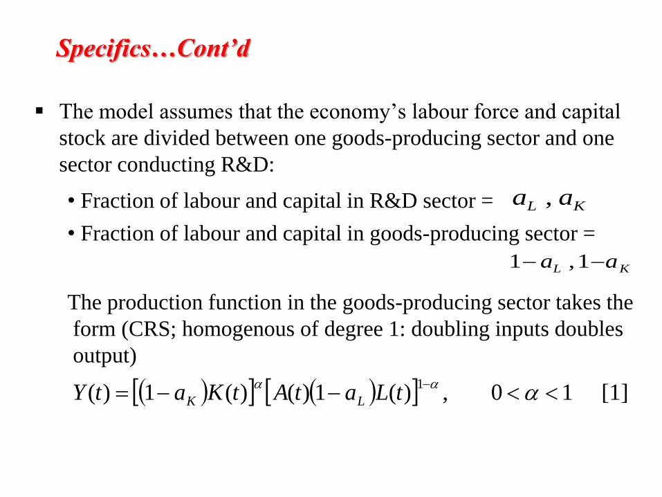
The model assumes that the economy‟s labour force and capital

stock are divided between one goods-producing sector and one

sector conducting R&D:

• Fraction of labour and capital in R&D sector =

• Fraction of labour and capital in goods-producing sector =

The production function in the goods-producing sector takes the

form (CRS; homogenous of degree 1: doubling inputs doubles

output)

KL aa ,

KL aa 1,1

[1] 10,)(1)()(1)(1

tLatAtKatY LK

Specifics…Cont’d

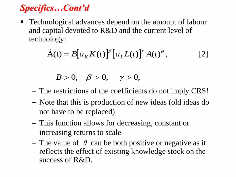
Technological advances depend on the amount of labour and capital devoted to R&D and the current level of technology:

– The restrictions of the coefficients do not imply CRS!

– Note that this is production of new ideas (old ideas do

not have to be replaced)

– This function allows for decreasing, constant or

increasing returns to scale

– The value of can be both positive or negative as it reflects the effect of existing knowledge stock on the success of R&D.

,0,0,0

[2] ,)()()((t)A

B

tAtLatKaB LK

Specifics…Cont’d

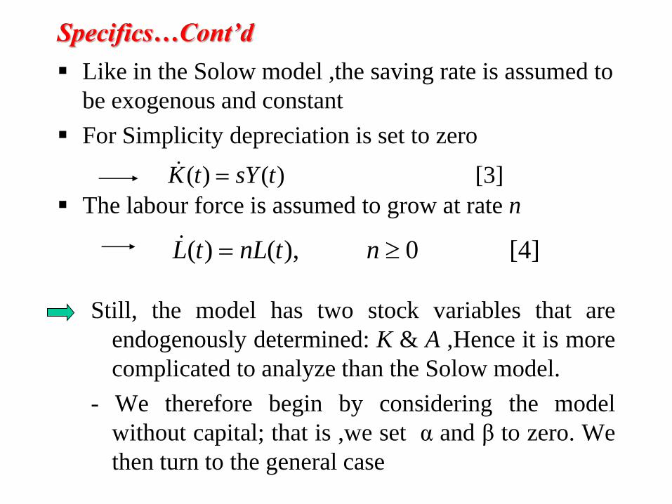
Like in the Solow model ,the saving rate is assumed to

be exogenous and constant

For Simplicity depreciation is set to zero

The labour force is assumed to grow at rate n

Still, the model has two stock variables that are

endogenously determined: K & A ,Hence it is more

complicated to analyze than the Solow model.

- We therefore begin by considering the model

without capital; that is ,we set α and β to zero. We

then turn to the general case

[3] )()( tsYtK

[4] 0 ),()( ntnLtL

II. The model without capital

The dynamics of knowledge accumulation

Where there is no capital, the production function for the goods sector becomes:

Output is proportional to A – hence the dynamics of A is of particular interest.

[5] )()1)(()( tLatAtY L

[7] )()()(

)()(

[6] )()()(

1

tAtLBatA

tAtg

tAtLaBtA

LA

L

Taking logs of both sides and differentiate w.r.t. to time gives

us the growth rate of the growth rate of A (the growth in

technological progress):**

The initial values of A and L determines the initial value of

, which determines the value but all depends on θ

[9] )()1()()(

[8] )()1()(

)(

2tgtngtg

tgntg

tg

AAA

A

A

A

Ag )(tg A

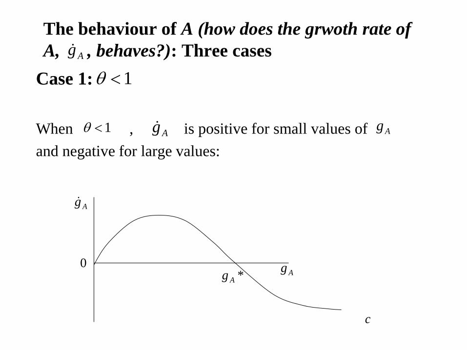
The behaviour of A (how does the grwoth rate of

A, , behaves?): Three cases

Case 1:

When , is positive for small values of

and negative for large values:

1

1 Ag Ag

*Ag Ag

Ag

c

0

Ag

There is a unique value of the growth rate of A, , where :i.e., the steady state is where

• Regardless of the economy‟s initial conditions converges

to [eg if the parameter values and the initial value of L and A imply (0)< , is positive; ie is rising ]

• The long-run growth rate of output per worker, , is an increasing function of the population growth.

• An increase in the fraction of the labor force devoted to R&D, and when θ<1, has a level effect (influences , Eqn 7) but no growth effect on the long run path of A [ie aL is not found in [eqn 10] but on Eqn 7].

*Ag

0Ag

[10] 1

01

0)1()(

*

*

2

ng

gn

ggndt

dg

A

A

AAA

Ag*Ag

*Ag

Ag

*AgAg

Ag Ag

.

This is a model of endogenous growth

• Output growth occurs because of technological growth

• Technology grows because new ideas are created and old

ideas don‟t depreciate

It‟s kind of odd that the growth of technology depends

on population growth

• This seems truer at larger scales, but not at smaller ones (ie

larger population larger chance of innovation)

Technological growth does not depend on the proportion of

people working in research and development

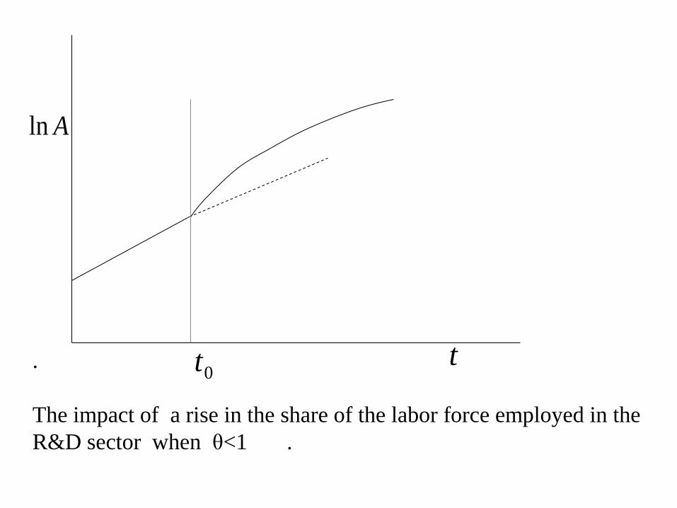
Although Eqn 7 says increase in aL immediately increase gA

owing to the limited contribution of the additional knowledge to

the production of new knowledge, this increase in the growth

rate of knowledge is not sustained (like saving rate in SS model,

shown in the next figure/slide)

Aln

t.

The impact of a rise in the share of the labor force employed in the

R&D sector when θ<1 .

0t

• So, an increase in the share of the population

working in R&D can produce a level effect on

technology and output

– But, no growth effect

• For example, the R&D in a war effort might

boost your output permanently, but would only

produce a transitory effect on its growth rate

– This sounds a lot like the U.S. in World War II

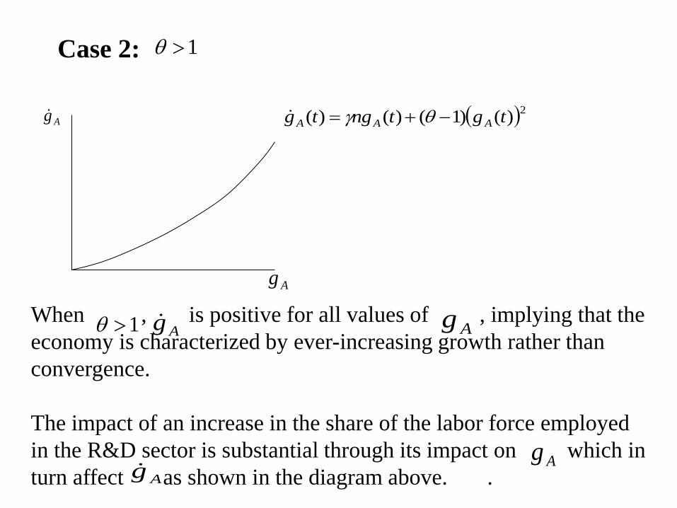
Case 2: 1

Ag

Ag

2)()1()()( tgtngtg AAA

When , is positive for all values of , implying that the

economy is characterized by ever-increasing growth rather than

convergence.

The impact of an increase in the share of the labor force employed

in the R&D sector is substantial through its impact on which in

turn affect as shown in the diagram above. .

1 Ag Ag

AgAg

• In this case, there is no steady-state growth

rate of technology

– The growth rate accelerates

• This implies that the overall economy never

reaches a steady-state either

– This is implausible, but shouldn‟t be completely

dismissed. Growth rates of developed countries

have been inching up over the decades.

• This is one type of fully endogenous model of growth

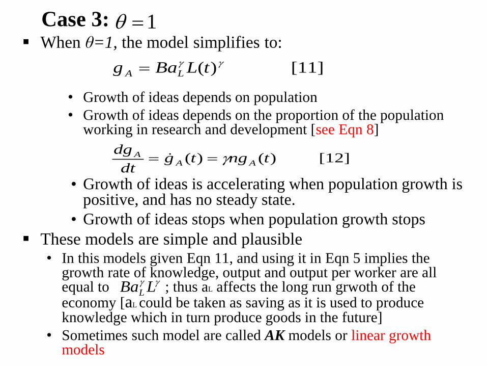
Case 3: When θ=1, the model simplifies to:

• Growth of ideas depends on population

• Growth of ideas depends on the proportion of the population working in research and development [see Eqn 8]

• Growth of ideas is accelerating when population growth is positive, and has no steady state.

• Growth of ideas stops when population growth stops

These models are simple and plausible • In this models given Eqn 11, and using it in Eqn 5 implies the

growth rate of knowledge, output and output per worker are all equal to ; thus aL affects the long run grwoth of the economy [aL could be taken as saving as it is used to produce knowledge which in turn produce goods in the future]

• Sometimes such model are called AK models or linear growth models

[11] )( tLBag LA

[12] )()( tngtgdt

dgAA

A

1

LBaL

.

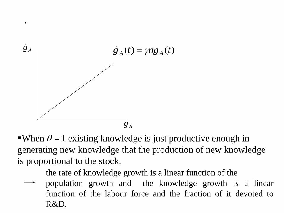
)()( tngtg AA Ag

Ag

When existing knowledge is just productive enough in

generating new knowledge that the production of new knowledge

is proportional to the stock.

the rate of knowledge growth is a linear function of the

population growth and the knowledge growth is a linear

function of the labour force and the fraction of it devoted to

R&D.

1

Since the output good in this economy has no use other than in

consumption, we can think of the resources devoted to R&D as

resources withdrawn from consumption, i.e. a form of saving.

resources devoted to R&D are useful in increasing future

consumptions rather than current consumption.

With this interpretation of as saving, as noted earlier the

model provides an example of a case where the saving rate may

affect long-run growth.

La

The Importance of Returns to Scale to Produced Factors:

The reason that these three cases have such different

implication is that whether θ is less than, greater than or

equal to 1, it determines whether there are decreasing

,increasing, or constant returns to scale to produced factors

of production.

The growth of labor is exogenous, and we have eliminated

capital from the model; thus

• knowledge is the only produced factor.

• There are constant returns to knowledge in goods production

→ Thus whether there are on the whole increasing, decreasing,

or constant returns to knowledge in this economy is

determined by the returns to scale to Knowledge in

knowledge production-that is , by θ

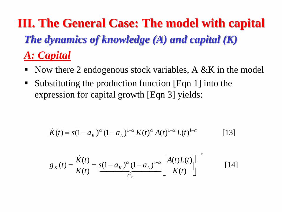
III. The General Case: The model with capital

The dynamics of knowledge (A) and capital (K)

A: Capital

Now there 2 endogenous stock variables, A &K in the model

Substituting the production function [Eqn 1] into the

expression for capital growth [Eqn 3] yields:

[14] )(

)()()1()1(

)(

)()(

[13] )()()()1()1()(

1

1

111

tK

tLtAaas

tK

tKtg

tLtAtKaastK

KC

LKK

LK

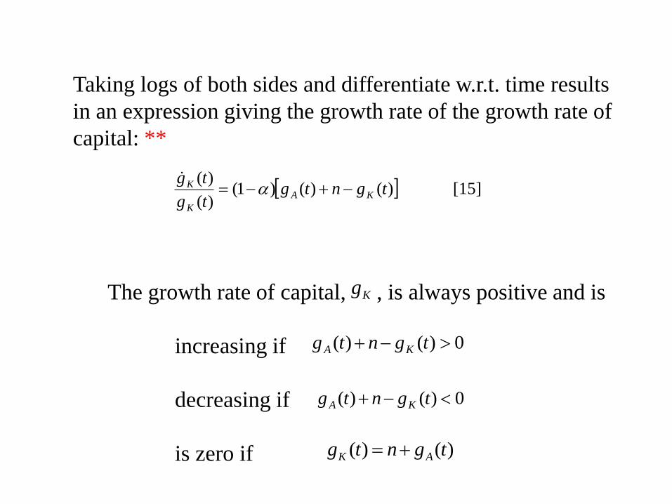
The growth rate of capital, , is always positive and is

increasing if

decreasing if

is zero if

[15] )()()1()(

)(tgntg

tg

tgKA

K

K

0)()( tgntg KA

0)()( tgntg KA

Taking logs of both sides and differentiate w.r.t. time results

in an expression giving the growth rate of the growth rate of

capital: **

)()( tgntg AK

Kg

Kg

Ag

0 AK gng

n

0Kg

0Kg

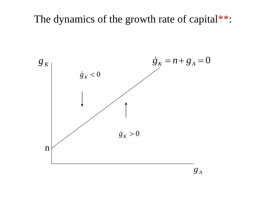
The dynamics of the growth rate of capital**:

B: Knowledge

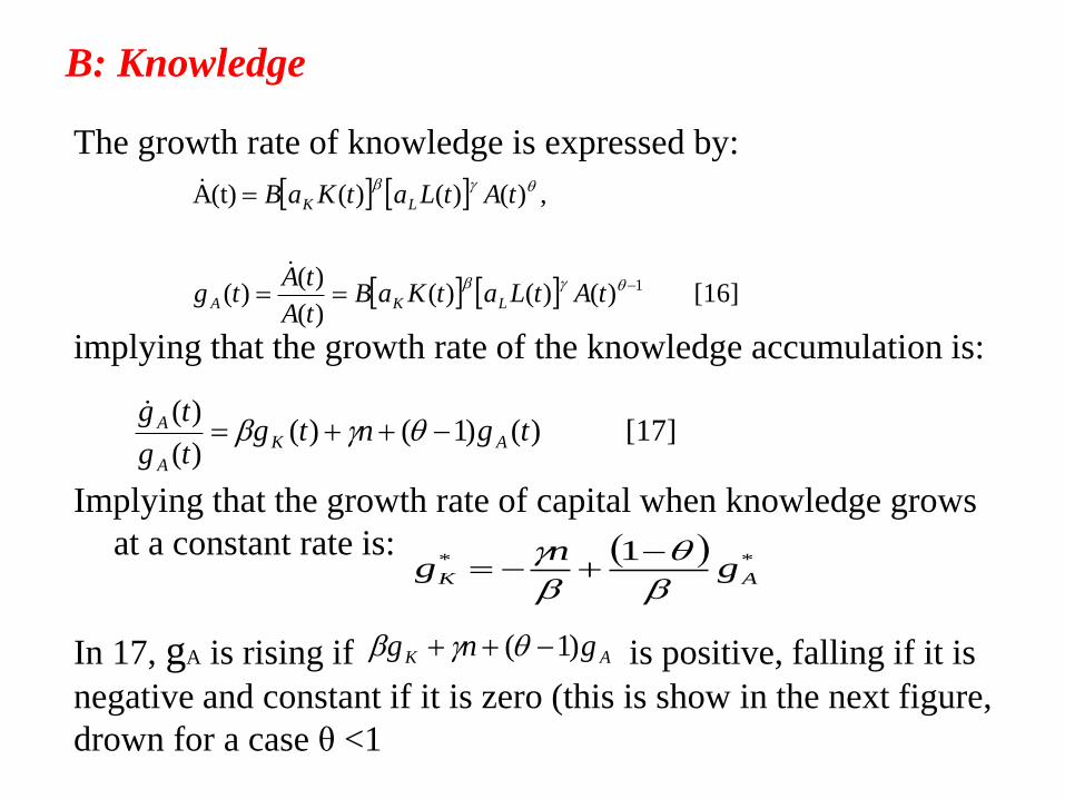
The growth rate of knowledge is expressed by:

implying that the growth rate of the knowledge accumulation is:

Implying that the growth rate of capital when knowledge grows

at a constant rate is:

In 17, gA is rising if is positive, falling if it is

negative and constant if it is zero (this is show in the next figure,

drown for a case θ <1

[16] )()()()(

)()(

,)()()((t)A

1

tAtLatKaBtA

tAtg

tAtLatKaB

LKA

LK

** 1AK g

ng

[17] )()1()()(

)(tgntg

tg

tgAK

A

A

AK gng )1(

Kg

Ag

0Ag

0Ag

The dynamics of the growth rate of knowledge:

n

(this case ) 1

0,

1

AAK gg

ng

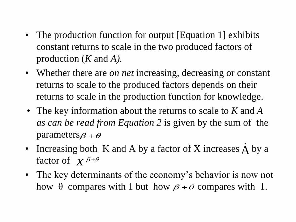
• The production function for output [Equation 1] exhibits

constant returns to scale in the two produced factors of

production (K and A).

• Whether there are on net increasing, decreasing or constant

returns to scale to the produced factors depends on their

returns to scale in the production function for knowledge.

• The key information about the returns to scale to K and A

as can be read from Equation 2 is given by the sum of the

parameters

• Increasing both K and A by a factor of X increases by a

factor of

• The key determinants of the economy‟s behavior is now not

how θ compares with 1 but how compares with 1.

X

A

• Case 1:

• if , is greater than 1 -the locus of points

where gA=0 [the previous figure] is steeper than the locus where

gK=0 [the one before the last one]: see in the diagram below

• The behavior of the growth rates of knowledge and capital when

implies that regardless of the initial level, these growth

rates converge to E in the diagram next - a level where they both

remain constant:

1

- In this equilibrium and are 0/ satisfy the equations

*Ag *

Kg

[18] 0 **** ngggng AKKA

[19] 0)1( ** AK gng

** 1AK g

ng

1 /1

1

Kg

Ag

0Ag

0Kg

0Ag

Case 1: The dynamics of the growth rates of knowledge and

capital when (n is positive):

n

Slope = 1/1

1

0Kg

0Ag

Slope = 1

0Kg

*Ag

*Kg

n

• Rewritings [18] for and substituting into [19] yields

• Combining these conditions give an expression for :

• In equilibrium (when A&K are growing at =n+ : – Then output will grow at rate [see Eqn1 &CRS assumption]

– Output per worker will grow at rate

– Long run growth is an increasing function of population

growth [from 21]

– The fractions of the labor force and capital stock devoted to

R&D hove no long-run effect on growth rates, but a level

effect [are not in 21 but are there on 16]

– The saving rate do not affect long-run growth rate but has a

level effect [again via aL]

*Ag

[21] )(1

* ng A

*Ag

*

Kg

[20] 0)1()( ** AA gg

*

Kg

*

Kg *Ag

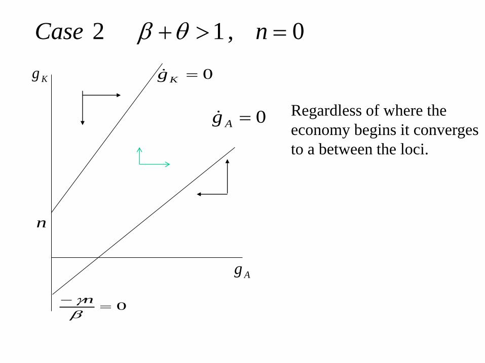
Case 2: The dynamics of the growth rates of

knowledge and capital when

–In this case the loci gA and gK are constant and diverge as

shows in the next figure.

–Regardless of where economy starts it eventually enters the

region between the two loci

–Once this occurs the growth rate of both A and K and hence

output grwoth rate increases continuously.

–This case is analogous to the case when θ exceeds 1 in the

simple model with no capital

1

0Ag

Kg

Ag

Regardless of where the

economy begins it converges

to a between the loci.

0,1 2 nCase

0Kg

0

n

n

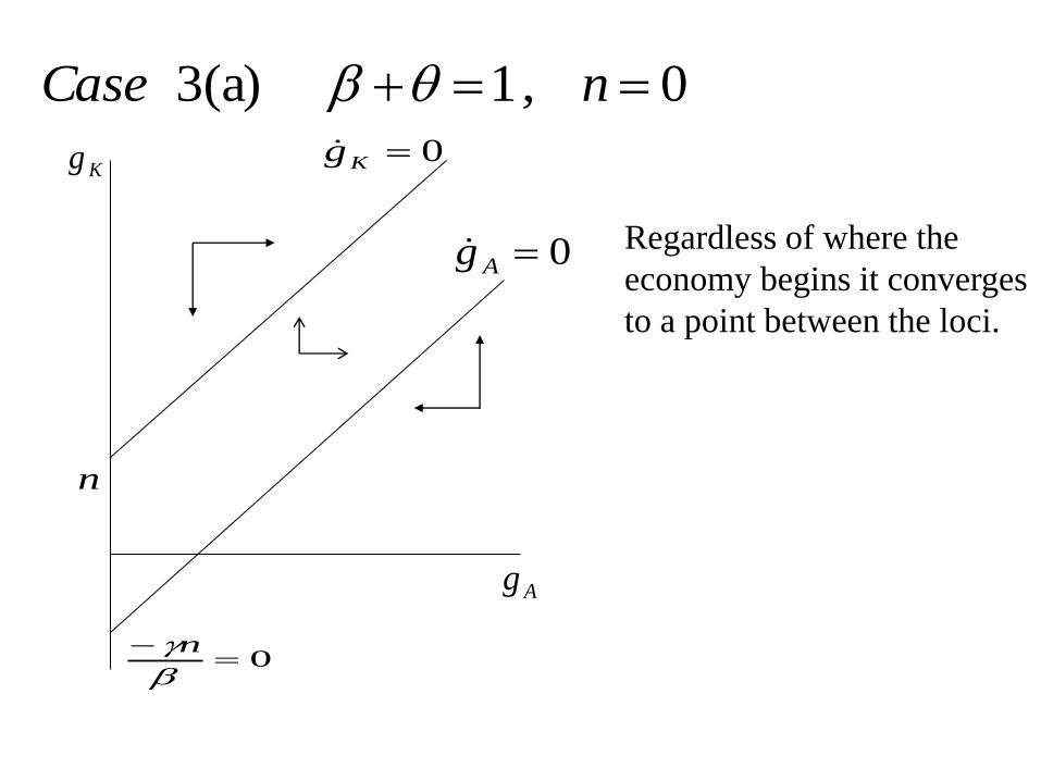
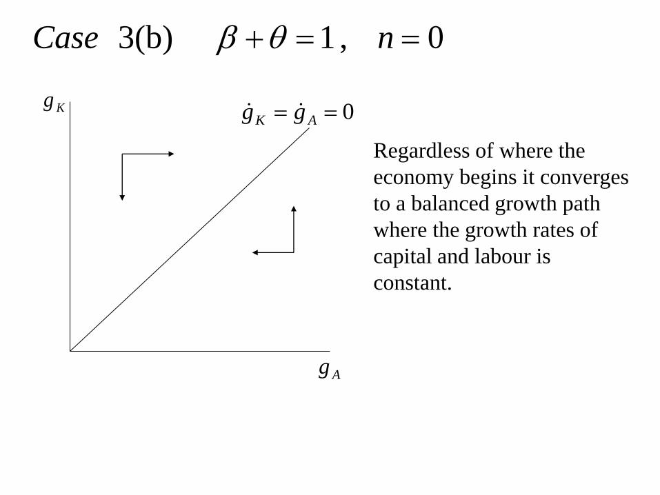
Case 3: The dynamics of the growth rates of

knowledge and capital when

–In this case (1-θ)/β equals 1 and hence the loci gA and gK have

the same slope (see next figure)

–In n is postive the gK.=0 line lies above gA =0 line and the

dynamics of the economy is similar to those when (θ+β) >1

(shown in panel a figure)

–When n is 0 on the other hand the two loci lie on to of each

other (shown in panel b of the figure next)

–The figure (panel b) shows regardless of where the economy

begins it converges to the balanced growth path

–As in the model with θ =1 and n=0 in the model without capital,

panel b doesn‟t tell us what balanced growth path the economy

converges to. (the model, however has a unique balance growh

path) –Romer (1990) model is good example (Nxt slide)

1

0Ag

Kg

Ag

Regardless of where the

economy begins it converges

to a point between the loci.

0Kg

0

n

n

0,1 3(a) nCase

0 AK gg Kg

Ag

Regardless of where the

economy begins it converges

to a balanced growth path

where the growth rates of

capital and labour is

constant.

0,1 3(b) nCase

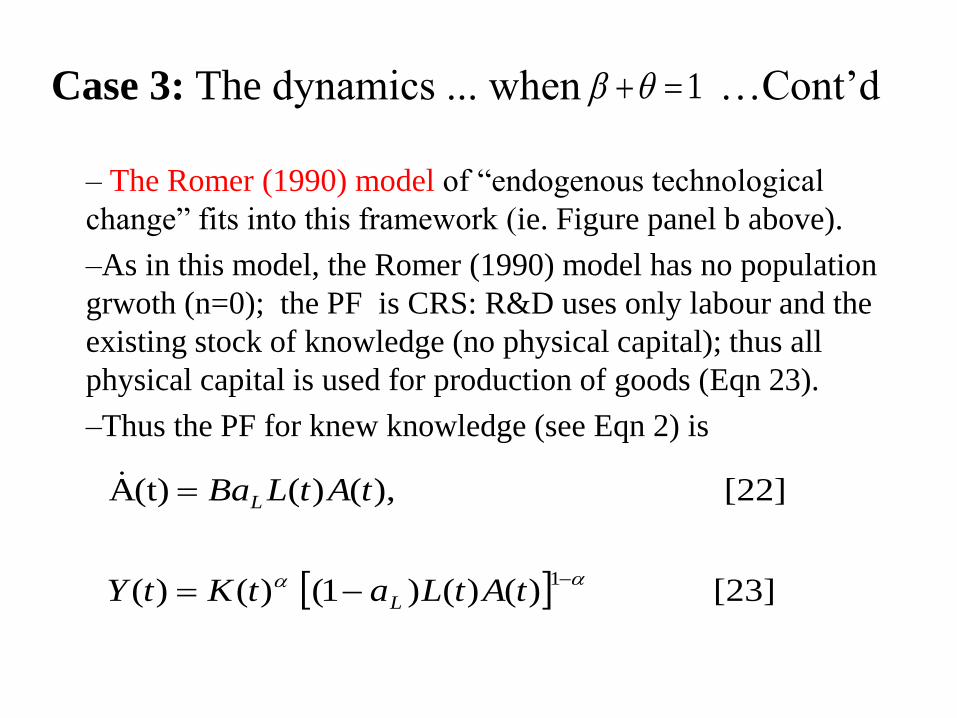
Case 3: The dynamics ... when …Cont‟d

– The Romer (1990) model of “endogenous technological

change” fits into this framework (ie. Figure panel b above).

–As in this model, the Romer (1990) model has no population

grwoth (n=0); the PF is CRS: R&D uses only labour and the

existing stock of knowledge (no physical capital); thus all

physical capital is used for production of goods (Eqn 23).

–Thus the PF for knew knowledge (see Eqn 2) is

1

[23] )()()1()()(

[22] ),()((t)A

1

tAtLatKtY

tAtLBa

L

L

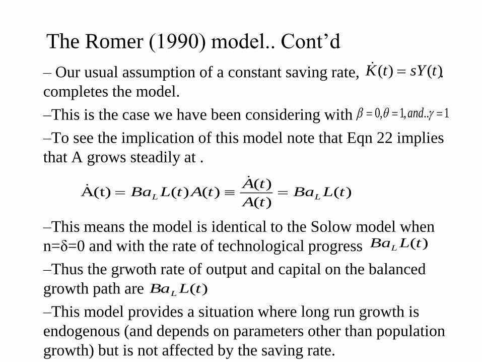
The Romer (1990) model.. Cont‟d

– Our usual assumption of a constant saving rate, .

completes the model.

–This is the case we have been considering with

–To see the implication of this model note that Eqn 22 implies

that A grows steadily at .

–This means the model is identical to the Solow model when

n=δ=0 and with the rate of technological progress

–Thus the grwoth rate of output and capital on the balanced

growth path are

–This model provides a situation where long run growth is

endogenous (and depends on parameters other than population

growth) but is not affected by the saving rate.

)()( tsYtK

)()(

)()()((t)A tLBa

tA

tAtAtLBa LL

1..,1,0 and

)(tLBaL

)(tLBaL

IV. The Nature of Knowledge and the Allocation

of Resources to R&D [Romer 1990 Model]

A. The Nature of Knowledge

Knowledge comes in many forms, from highly abstract

scientific results to highly applied every-day solutions found

by each and every individual.

Knowledge in all its forms between basic scientific research

to product specific development plays a fundamental role in

economic activity.

There is, however, no reason to believe that the

accumulation process of different types of knowledge to be

the same.

Still, all types of knowledge share on essential feature:

non-rivalry

The Nature of Knowledge: Non-rivalry

The use of a specific item in one activity does not prevent its simultaneous use in any other activity.

This feature of knowledge has two important implications:

1. The production and allocation of knowledge cannot be completely governed by competitive market forces:

– since the marginal cost of supplying knowledge to an additional user is zero the rental price of knowledge in a competitive market is also zero, implying that the creation of knowledge would not be motivated by private economic incentives.

2. Returns to scale:

– If a non-rival input has productive value, then output cannot be a constant-returns-to-scale function of all its inputs taken together.

– The standard replication argument used to justify homogeneity of degree one does not apply because it is not necessary to replicate non-rival inputs.

The Nature of Knowledge : Excludability

A good is excludable if it is possible to prevent others from using it.

Although all knowledge is non-rival the possibility to exclude others

from using it varies with the type of knowledge:

– Complex knowledge has a lower propensity to „leak‟

– Different type of knowledge is protected by different types of property rights.

The degree of excludability are likely to have strong influences on

how the production and allocation of knowledge depart from a

competitive market equilibrium:

– With no excludability – private returns are small

– With strong excludability – private returns are large due to monopoly rents.

B. The Determinants of the Allocation of resources to R&D

What determines the fraction of inputs devoted to R&D, i.e. the

exogenously parameters and ?

– Support for basic scientific research by governments and

charities

• Done by research centers/universities

• Available freely and thus need to be subsidized

– Private incentives for R&D and innovation

• Intellectual property rights allows for temporary monopolies

– Positive externality: New knowledge are created that will become

available for others after some time

– Positive externality: Consumers consume qualitatively upgraded goods

– Negative externality: Some producers of old technologies are driven out

of business.

– The production of new knowledge has a positive effect on production of

additional knowledge, i.e. stimulates further technological progress

La Ka

- Alternative Opportunities for talented individuals

• Baumol (1990) and Murphy, Shleifer and Vishny (1991) observe that major innovations and technology advances are often results of the work of extremely talented individuals.

• Talented individuals have many opportunities to choose from and historically such individuals have made careers in rent-seeking rather than socially productive activities.

• The probability that talented individuals choose socially productive careers is largely dependent on the opportunities to gain private economic returns to these activities.

B. The Determinants of the Allocation to R&D..... Cont’d

B. The Determinants of the Allocation to R&D..... Cont’d

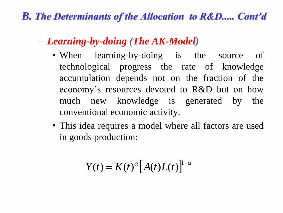
– Learning-by-doing (The AK-Model)

• When learning-by-doing is the source of

technological progress the rate of knowledge

accumulation depends not on the fraction of the

economy‟s resources devoted to R&D but on how

much new knowledge is generated by the

conventional economic activity.

• This idea requires a model where all factors are used

in goods production:

1)()()()( tLtAtKtY

B. The Determinants of the Allocation to R&D..... Cont’d

– The simplest case of learning-by-doing is when

learning occurs as a side effect of the production of

new capital (& hence technology is labour-

augmenting).

– In this case knowledge accumulation is a function of

the increase in capital or capital/Labour ratio:

1)1(1 )()()()(

)()(

tLtKBtKtY

tBKtA

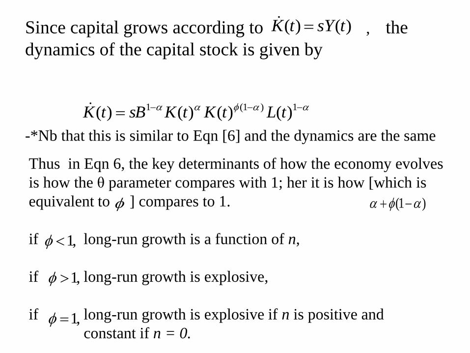
Thus in Eqn 6, the key determinants of how the economy evolves

is how the θ parameter compares with 1; her it is how [which is

equivalent to ] compares to 1.

if long-run growth is a function of n,

if long-run growth is explosive,

if long-run growth is explosive if n is positive and

constant if n = 0.

Since capital grows according to , the

dynamics of the capital stock is given by

-*Nb that this is similar to Eqn [6] and the dynamics are the same

1)1(1 )()()()( tLtKtKsBtK

)()( tsYtK

)1(

,1

,1

,1

When and n = 0 the production function becomes

,1

)()( tbKtY

Capital accumulation is then given by )()( tsbKtK

• Both output and capital is growing at constant rate (sb)

• Long-run growth depend on the saving rate

The contribution of capital extends beyond its conventional

contribution to the economy in the goods production since

capital also contributes to the development of new ideas.

Read the Implication of such Endogenous grwoth models when

framed in a Ramsey (endogenous saving) set up. Romer, 2001,

2nd edn, P. 122.

V. Endogenous growth theory and the

central questions of growth theory

What do models of R&D and knowledge accumulation

say about the issues of economic growth over time and

across countries?

Worldwide growth over time

• The growth of knowledge appear to be the central

reason that output and living standards are

significantly higher today than a century ago

• Results of empirical growth accounting points to the

importance of the „Solow residual‟ which may reflect

technological progress.

Endogenous growth theory and the central

questions of growth theory (cont.)

• Cross-country differences in real income

– The relevance of endogenous growth models are less obvious

• If income differences are attributed to lags in technological diffusion, the lags in the diffusion of knowledge from rich to poor countries that are needed to account for observed income differentials are extremely long, more than 100 years.

• Since technology and knowledge are largely non-rival it is difficult to explain why poor countries should not have access to the same technology as rich countries.

• It seems like it is the lack of ability to adopt advanced technologies rather than poor access to them that differ between poor and rich countries (see the Nelson and Phelp‟s (1966) model)

• Poverty and prosperity is related to whatever factors that allow some countries (and individuals) to take better advantage of advanced technologies [Institution! Politics!Vision! etc see PE Lecture).

END END END

Part B: Models with human

capital

I.Overview

In this section we investigate the role of human capital

in economic growth.

Investments in human capital, and hence growth in

human capital, has been seen in the literature as an

endogenous engine of growth.

Human capital investment in this framework typically

includes not only schooling but also on the job

training.

We start by incorporating human capital in the Solow

model.

II. The Solow model with human capital

We have already discussed in Lecture 1, the Augmented

Solow-Swan model – the Solow model with human capital.

That model can also be taken as a variety of endogenous

grwoth model (so refer Lecture 1)

It had to be recall that that model is based on the classic works

of Mankiw, Romer and Weil(1992).

Recall also further that the Mankiw et al (1992) „Augmented

Solow-Swan model” has helped to solve the puzzle of high

share of capital from the model (about 68%) which doesn‟t

tally with the reality of capital share (about 33%) using a

“Growth Accounting Exercise”.

In the rest of the lecture, thus, we will focus on another

human capital-based endogenous growth model attributed to

Uzawa (1961) and Lucas (1988) – the Uzawa-Lucas Model

The Lucas Model

{See Next Slide: “the Lucas Model”}