advanced coexistence technologies for radio optimisation
TRANSCRIPT
ICT 257626 ACROPOLIS Date: 04/07/2014
ICT-ACROPOLIS Deliverable D14.3 1/84
Advanced coexistence technologies for radio optimisation in
licensed and unlicensed spectrum
(ACROPOLIS)
Document Number D14.3
Assessment of interference in cognitive radio-based networks
Contractual date of delivery to the CEC: 30/01/2013
Actual date of delivery to the CEC: 15/01/2013, revised 04/07/2014
Project Number and Acronym: 257626 - ACROPOLIS
Editor: L. Goratti (JRC), G. Baldini (JRC)
Authors: L. Goratti (JRC), G. Baldini (JRC), P. Chawdhry
(JRC), O. Holland (KCL), A. Bantouna (UPRC), S.
Bovelli (EADS)
Participants: UPRC, KCL, JRC, EADS
Workpackage: WP14
Security: PU
Nature: Report
Version: 1.1
Total Number of Pages: 84
Abstract:
A survey of interference issues in spectrum sharing is presented, particularly on aggregate
interference. It is shown that the distribution of aggregate interference power can be
modelled with a family of heavy tail ‘stable distributions’. The report also reviews some of
the landmark practical work in Europe for CEPT and OFCOM based on measurements in
the context of spectrum sharing in the television white space. The need to protect
incumbents from harmful interference from white space devices has led to setting the
protection ratios for DVB-T receivers of digital terrestrial television users and the wireless
microphones of the PMSE community. These protection ratios will form the basis of
regulatory limits in future while considering the allowable use of white space technologies
by secondary users while minimising risk of interference to primary users.
Keywords: Aggregate interference, cognitive radio, white spaces, commons, stochastic
geometry, simulation tools.
Ref. Ares(2014)2261702 - 08/07/2014

ICT 257626 ACROPOLIS Date: 04/07/2014
ICT-ACROPOLIS Deliverable D14.3 2/84
Document Revision History
Version Date Author Summary of main changes
0.1 07.06.2011 JRC Initial structure of the document, ToC
developed
0.2 31.08.2011 JRC New structure
0.3 19.10.2012 JRC, EADS, KCL, UPRC Update structure and work sharing
0.4 09/12/2012 JRC Update structure and contributions
0.5 12/12/2012 JRC Update to the sections
0.6 14/12/2012 JRC Abstract and executive summary added
0.7 16/12/2012 KCL Document update and contributions
0.8 18/12/2012 JRC,UPRC Document update and contributions
0.9 10/01/2013 JRC Document update
0.91 14/01/2013 JRC, KCL, UPRC, EADS Document update and contributions
0.92 18.01.2013 JRC Editorial updates
1.0 18.01.2013 JRC, KCL, UPRC, EADS Final revision after review by Executive
Committee
1.1 03.07.2014 JRC, KCL Revised after comments from Project Final
Review

ICT 257626 ACROPOLIS Date: 04/07/2014
ICT-ACROPOLIS Deliverable D14.3 3/84
Executive Summary
With exponential growth in wireless communication technologies, there is increasing
pressure on the regulators to adopt modern spectrum management techniques where
spectrum sharing is a key paradigm. However, spectrum sharing (over frequencies, time and
space) increases the risk of harmful interference the prevention of which is a major task of
the regulators. This report addresses the key issues of interference in the presence of
secondary users.
Since the early 2000’s the concept of cognitive radio, aimed to enable efficient use of the
spectrum, has gained currency in the academia and industry. Today cognitive radio is seen
as a key enabling technology for spectrum sharing. The first and second digital divided that
has followed the switch-over from analogue to digital TV, promises to release valuable
portions of spectrum in the UHF band, some of which may be available for spectrum
sharing.
Spectrum regulatory authorities are now devising regulatory framework for spectrum
sharing. However, the problem of interference in spectrum sharing is a major challenge, and
especially the issue of aggregate interference given the proliferation of wireless services and
devices and the fact that regulatory concepts such as TV White Space access (e.g., channel
availabilities) are generally only assessed based on the assumption of a single interferer.
This report is devoted to a review of the most advanced analytical and simulation
techniques that can be used to model aggregate interference, as well as measurement
campaigns by the regulators on protection of the incumbents from interference in the TV
white spaces.
Chapter 2 reviews opportunistic spectrum access which creates the opening of underutilized
portions of the licensed spectrum for reuse, provided that the transmissions of secondary
radios do not cause harmful interference to primary users (PUs). For secondary users to
accurately detect and access the idle spectrum, CR has been proposed as the enabling
technology for spectrum sharing.
Spectrum sharing is however challenging due to the uncertainty associated with the
aggregate interference in a wireless network. Such uncertainty can be resulted from the
unknown number and location of interferers and unknown location of the primary signals as
well as channel fading, shadowing, and other environment-dependent conditions.
Therefore, it is crucial to incorporate such uncertainty in the statistical model of the
aggregate interference in order to quantify its effect on the primary network system
performance. A unifying framework for characterizing the network interference is found
useful in investigating a variety of issues involving the aggregate interfering power
generated asynchronously in a wireless environment subject to path-loss, shadowing, and
multipath fading.
Chapter 3 considers operational scenarios selected for the characterization of the aggregate
interference which are closely connected with the different forms of spectrum-sharing that
are currently being considered. Spectrum sharing can be distinguished on the basis of three
principal parameters: time, frequency and space.
Chapter 4 is the theoretical heart of the report. It presents an overview of some
fundamental aspects of modelling the aggregate interference in wireless systems which
ICT 257626 ACROPOLIS Date: 04/07/2014
ICT-ACROPOLIS Deliverable D14.3 4/84
plays a major role in the management and optimization of wireless networks since
aggregate interference in a shared wireless channel has a number of implications on
network performance.
Depending on the radio technology used, narrowband or ultra wideband, the type of
environment where the network has to operate (urban or rural), network performance may
vary quite dramatically. In a realistic environment, the location of the wireless devices with
respect to the receiver, the time of arrival of the received packets and the different levels of
received power affect the performance of a wireless link.
The capture model, where a transmitted packet is received correctly by the intended
receiver despite collisions with concurrent transmissions, has been successfully applied to
model realistic performance of packet switched radio networks under various transmission
schemes and propagation effects.
Stochastic geometry provides excellent means to devise the performance of packet
switched radio networks in which devices generate harmful interference affecting each
other’s behaviour. The core contribution of this approach consists of modelling the nodes of
a wireless network as a point process (PP). The section reviews how stochastic geometry is
helpful for modelling the behaviour of a wireless network where the aggregate interference
assumes the key role.
The assumption of the Poisson distribution of the devices over space and the Gaussian
modelling of the distribution of the aggregate interference power provided already a good
insight of the network behaviour. This has represented a fundamental step that bridged
together the systemic approach with the physics of the radio signal propagation.
Modelling the distribution of the aggregate interference power is considered. In particular,
the distribution of the aggregate interference power generated by a Poisson field of
interferers belongs to the family of stable distributions. Stable distributions assume an
important role when modelling the distribution of the aggregate interference power
generated by an infinite number of nodes distributed over space according to a PPP.
The computation of the distribution of the aggregate interference power is particularly
important when typical propagation effects such as fading and shadowing are superimposed
on top of the link distance loss. Three cases are considered: Rayleigh fading, Nakagami-m
fading and shadowing.
A reference scenario explains how the distribution of the aggregate interference power is
calculated. It shows that nodes are distributed over space according to a point process with
respect to the common receiver which is placed at the origin of the reference system.
Despite the number of nodes can be high, what really matters is the number of active
transmitters. The transmission of each device can arrive from different distances and
encounter different levels of fading and shadowing.
Existing literature shows different approaches to the way the aggregate interfering process
is modelled. When the interferers are distributed according to a PPP, the distribution of the
aggregate interference power belongs to the family of stable distributions with location
parameter δ=0 and with the other parameters that depend on the characteristics of the
radio signal, the fading and the shadowing. These approaches are based on i) the theory of
shot noise and elements of stochastic geometry; ii) modelling based on the LePage series
representation of the aggregate interference and iii) an approach relying more on standard
ICT 257626 ACROPOLIS Date: 04/07/2014
ICT-ACROPOLIS Deliverable D14.3 5/84
probability theory. The derivation of the distribution of the aggregate interference is helpful
for determining the probability of detecting the transmission of a PU from the point of view
of a CR network.
Chapter 5 is dedicated to review some of the simulation tools that can be used to quantify
the aggregate interference power generated by cognitive radio networks over a primary
link. A number of simulators are nowadays available including licensed and unlicensed
software tools. Licensed software include Matlab and Opnet for example. Unlicensed tools
include ns-2, ns-3, OMNET++ and SEAMCAT. All of them have pros and cons however,
SEAMCAT is the official tool used by ECC/CEPT to carry out compatibility studies for
regulatory proposals in Europe. The other mentioned simulators find applications in
modelling many different aspects of the behaviour of wireless and wired networks.
Based on Monte-Carlo simulation method, SEAMCAT allows simulating different
interference scenarios with the purpose of addressing compatibility studies between
different radio technologies operating in the same or adjacent frequency bands. It is used
for co-existence studies in terms of the determining the transmitter/receiver mask,
unwanted emissions (spurious out-of-band), blocking/selectivity, etc. For studies on
spectrum sharing, SEAMCAT can be used for Monte-Carlo simulations of the interference
produced by CR devices operating in TV White Spaces when the interference is measured at
the location of the victim receiver (DVB-T or PMSE).
Chapter 6 gives a summary of the main results on the aggregate interference power
generated by CR devices.
Chapter 7 considers practical issues in the deployment of cognitive radio, such as
standardization, regulation and measurement of interference and protection ratios.
Technical standards are set to follow the regulations, including emission requirements,
interaction with a geolocation database in the case of TV White Space, etc. A good example
of this is the IEEE 802.22 standard which interacts closely with the regulatory trend.
Following the decision in the US by the FCC to open up significant parts of the TV white
spaces for shared use, spectrum regulators in other parts of the world are considering
similar initiatives. The FCC selected a value of the maximum transmit power for devices
operating in the White Spaces in unlicensed fashion. The FCC also defined the so called
erosion margin, which quantifies how much the TV service can degrade and thus the
tolerable amount of interference that CR devices can inject in TV bands. A zero erosion
margin would imply zero white spaces. This margin is particularly important as it allows
determining how far the CR devices (referred to as White Spaces Devices) have to be from
television receivers, taking into account in-band interference and the interference caused by
transmissions on adjacent channels.
In the European context, the CEPT/ECC produced its landmark report ECC159 which
addresses the technical and operational requirements for the use of cognitive radio in TV
white space in 470-790 MHz band. The report considers the use of sensing and geolocation-
based approaches to minimise risk of harmful interference to the incumbents. The following
incumbent protection cases are considered: digital terrestrial television broadcasting,
Programme Making and Special Events (PMSE), radio astronomy (RAS), aeronautical radio
navigation (ARNS), mobile/fixed services in bands adjacent to the band 470-790 MHz.
ICT 257626 ACROPOLIS Date: 04/07/2014
ICT-ACROPOLIS Deliverable D14.3 6/84
At the national level, the UK’s OFCOM authorised in 2011 the Cambridge Trials on TV White
Space by a consortium of stakeholders to carry out field tests on the provision of services
such as rural broadband and to carry out measurements of several aspects, including:
- Protection of wireless microphones by the PMSE community
- Performance of TV white space base station for mobile and fixed broadband
applications
- Measurements on DVB-T protection ratios in the presence of interference from
white space devices.
In order to protect PMSE, relevant EIRP restrictions need to be applied on WSDs operating
in the geographic cells around the PMSE events. The protection approach is to limit the
interference at the PMSE receiver such that the sensitivity of the equipment is not degraded
beyond an acceptable margin. To achieve this, the interference from WSD, weighted by the
receiver ACS value should be in the range below the receiver’s noise floor.
The tests in the Cambridge Trial indicated that protection ratio values for both the high and
low power wanted signals are different; the worse adjacent channel protection ratio for the
-30dBm wanted signal is as a result of the receiver being overloaded (both wanted and
interfering signal powers are large in this case). It was found that the adjacent channel (+-
10MHz) minimum protection ratio is better than 55dBm for the non-overloaded case,
irrespective of the waveform used. The worst co-channel protection ratio is around 6dB.
In the presence of cognitive radio, specifically of the white space devices in the UHF band,
protection of Digital Terrestrial Television (DTT) receivers is required to ensure the quality of
DVB-T reception is free from unwanted interference from WSD signals in the adjacent UHF
bands.
Tests were carried out by BBC on a range of candidate technologies and assessed DVB-T
receiver performance in the UK context [132]. Fourteen popular models of commercially
available receivers were tested representing integrated digital television (IDTV), set top
boxes (STBs) and programmable video recorders (PVRs). The interference from WSDs was
generated through a vector signal generator to replay a waveform recorded from candidate
WSD radio technology.
The results of these tests show a considerable variation in performance of DTT receives.
Whereas high-end receivers appeared to be fairly resilient to interference from WSD signals,
other receivers were found to be vulnerable to the WSD waveforms used in the tests.
Broadcast-like signals (e.g. LTE base station at 100% traffic) were dealt with by the receivers
without interference. However, burst-like signals (e.g. low traffic CPE signals) result in up to
a 30dB degradation in protection ratios.
As a consequence of the BBC tests, they recommend the use of a highly conservative
protection ratio values in the UK in order to protect the majority of existing consumer grade
DVB-T receivers (largely in the form of low cost set-top boxes used to adapt old analogue TV
receivers to DTT reception). The authors concluded that the geolocation database approach
to TVWS was feasible provided that the database could take into consideration the various
WS technologies and the predicted field strength at the DTT receiver location.
ICT 257626 ACROPOLIS Date: 04/07/2014
ICT-ACROPOLIS Deliverable D14.3 7/84
Table of Contents
1. Introduction ................................................................................................... 8 2. Wireless interference in Cognitive Radio networks ...................................... 10 3. Operational scenarios for interference in cognitive radio systems ............... 12 3.1 Opportunistic Secondary Spectrum Access: TV White Spaces ........................... 13 3.2 Hierarchical Sharing with Equipment Under a Single Entity: Femtocells and Related
Examples ........................................................................................................ 15 3.2.1 Scenario 1: Ad-hoc deployment ............................................................. 15 3.2.2 Scenario2: Opportunistic capacity extension ............................................ 17
3.3 Shared Use of Licensed Spectrum in Underlay Mode ....................................... 20 3.3.1 Ultra-Wide Band ................................................................................... 21 3.3.2 Interference Threshold .......................................................................... 23
3.4 Spectrum Commons and Related Models: Interference among Secondary Systems
..................................................................................................................... 24 3.4.1 In Opportunistic Secondary Spectrum Access Scenarios: TV White Spaces .. 24 3.4.2 In Conventional Unlicensed Spectrum: ISM bands .................................... 24 3.4.3 In Unlicensed bands: Use of Opportunistic Wi-Fi Networks for Resolving
Interference among different RATs ................................................................. 25 4. Models of Wireless Interference ................................................................... 27 4.1 Validity of Gaussian modelling for the interference ......................................... 28 4.2 Stable distributions ..................................................................................... 30 4.2.1 Useful facts ......................................................................................... 34 4.2.2 Probability of detecting the primary transmission without interference ........ 36
4.3 Spatial interference model ........................................................................... 37 4.3.1 Aggregate interference based on Poisson distribution ................................ 38 4.3.2 Aggregate interference based on Binomial point processes ........................ 48 4.3.3 Probability of detecting the primary transmission with interference ............. 50
4.4 Cluster-based models ................................................................................. 52 5. Simulation tools to model interference in cognitive radio networks. ............ 54 6. Advantages/Disadvantages of the reviewed models .................................... 56 7. Standardization Perspective ......................................................................... 57 7.1 Limits on the aggregate interference ............................................................. 58 7.2 TV White Spaces estimation in the USA ......................................................... 58 7.3 TV White Spaces in the European Context ..................................................... 59 7.4 OFCOM Cambridge Trials on TV White Spaces ................................................ 60 7.5 Protection of PMSE Applications .................................................................... 61 7.5.1 PMSE Receiver Performance and Protection Ratios .................................... 63
7.6 Protection of DVB-T Receivers ...................................................................... 65 8. Conclusions .................................................................................................. 70 Appendix. A short tutorial on stochastic geometry ........................................... 72 9. References ................................................................................................... 75

ICT 257626 ACROPOLIS Date: 04/07/2014
ICT-ACROPOLIS Deliverable D14.3 8/84
1. Introduction
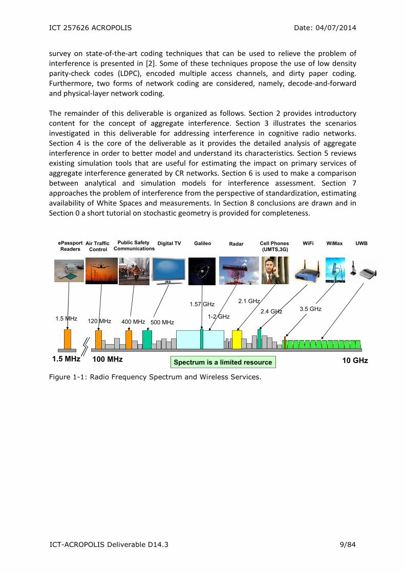
Radio waves are present throughout our environment to provide a number of wireless
services like radio, TV, cellular communications, wireless internet, radar, SATNAV, among
others. As shown in Figure 1-1, what initially looked like a vast expanse of radio spectrum
today looks instead very crowded. During the past decade, there has been an explosive
growth in mobile/wireless communications and other systems that are sharing the
spectrum. Current estimations predict that there will be more than 4.2 billion mobile
subscribers worldwide, which means 1 billion of new subscribers in only 3 years. In addition,
almost all mobile network operators are now offering data services in order to create new
sources of revenue.
The perspective of wireless communications is to maintain the promise of ubiquitous
connectivity, thanks to a variety of wireless systems such as Wi-Fi, WiMAX, and the third
and fourth generations of cellular networks. On the other hand, mobile subscribers can use
a variety of devices, ranging from smartphones to laptops. The surge in mobile and wireless
access will become important in any kind of environment. This includes rural areas, where
the endeavour of enabling broadband access (likely through wireless means and one future
option) will load the spectrum, and inside cities, where the high density of users and their
associated activities trigger the demand for high data rates. Such high proliferation of
wireless services over a finite spectrum will lead to its shortage in the near future.
A possible solution that could aid circumventing the shortage of radio spectrum is cognitive
radio (CR). First conceived in [1], CR is a very broad concept in which wireless devices might
be able to learn from experience and finely tune their transmission parameters based on the
scenario where they operate to allow spectrum access in a more flexible way with respect to
what is in force today. In a few words, CR should be able to empower wireless devices with
the feature to access the spectrum whenever there is a resource underutilized or not used
at all. Although CR constitutes a very appealing concept, it is clear that the proliferation of
wireless devices trying to access the spectrum whenever they need, and the opportunistic
spectrum access capabilities which CR might facilitate, could easily cause harmful
interferences to license owners in various spectrum bands.
This deliverable focuses first on the identification of the relevant operational scenarios for
the sake of modelling interference. Afterwards it provides the detailed analysis of the
aggregate interference in wireless networks, tailored to the specific case of CR devices
affecting the performance of primary (licensed) transmissions. In addition, in the attempt to
make a self-contained document, not only is presented a thorough but non-exhaustive
analysis of the aggregate interference but also a short tutorial on the stochastic geometry
that is the foundation of such techniques. Simulation tools are also reviewed for the sake of
completeness.
The problem of modelling aggregate interference in wireless networks is not new, and it has
been addressed in many different ways throughout the literature of mobile and wireless
communications. Consequently, it is worth mentioning that several techniques have been
developed to mitigate this problem. In essence, interference, and the better management
there, is the key reason why many multiple access techniques are developed. For instance, a
ICT 257626 ACROPOLIS Date: 04/07/2014
ICT-ACROPOLIS Deliverable D14.3 9/84
survey on state-of-the-art coding techniques that can be used to relieve the problem of
interference is presented in [2]. Some of these techniques propose the use of low density
parity-check codes (LDPC), encoded multiple access channels, and dirty paper coding.
Furthermore, two forms of network coding are considered, namely, decode-and-forward
and physical-layer network coding.
The remainder of this deliverable is organized as follows. Section 2 provides introductory
content for the concept of aggregate interference. Section 3 illustrates the scenarios
investigated in this deliverable for addressing interference in cognitive radio networks.
Section 4 is the core of the deliverable as it provides the detailed analysis of aggregate
interference in order to better model and understand its characteristics. Section 5 reviews
existing simulation tools that are useful for estimating the impact on primary services of
aggregate interference generated by CR networks. Section 6 is used to make a comparison
between analytical and simulation models for interference assessment. Section 7
approaches the problem of interference from the perspective of standardization, estimating
availability of White Spaces and measurements. In Section 8 conclusions are drawn and in
Section 0 a short tutorial on stochastic geometry is provided for completeness.
1.57 GHz
Spectrum is a limited resource100 MHz 10 GHz
400 MHz 500 MHz
2.1 GHz
1-2 GHz120 MHz
Air Traffic
Control
Public Safety
CommunicationsDigital TV Radar Cell Phones
(UMTS,3G)
Galileo WiFi UWBWiMax
2.4 GHz 3.5 GHz
1.5 MHz
1.5 MHz
ePassport
Readers
Figure 1-1: Radio Frequency Spectrum and Wireless Services.

ICT 257626 ACROPOLIS Date: 04/07/2014
ICT-ACROPOLIS Deliverable D14.3 10/84
2. Wireless interference in Cognitive Radio networks
With the emergence of new wireless applications and devices, there is a dramatic increase
in the demand for radio spectrum. Due to the scarcity and the under-utilization of assigned
spectrum, government regulatory bodies such as the U.S. Federal Communications
Commission (FCC) have started to review their spectrum allocation policies [3][4].
Conventional rigid spectrum allocation forbids flexible spectrum usage that severely hinders
efficient utilization of scarce spectrum since bandwidth demands vary along time and space
dimensions. Therefore, opportunistic spectrum access together with a CR technology has
become a promising solution to resolve this problem [6]-[9].
Opportunistic spectrum access creates the opening of underutilized portions of the licensed
spectrum for reuse, provided that the transmissions of secondary radios do not cause
harmful interference to primary users (PUs). For secondary users to accurately detect and
access the idle spectrum, CR has been proposed as the enabling technology [6][7][9]. For
example, if a communication channel is active between the primary and secondary
networks, the busy channel assessment can be based on the detection of a preamble shared
between the primary and secondary networks or on the energy sensing of the primary
network radio signals [10]-[12]. Moreover, the CR network can implement a detect-and-
avoid protocol where the transmission power levels of the CR devices are set based on the
sensed power of the primary network signals.
Spectrum sharing is however challenging due to the uncertainty associated with the
aggregate interference in the network. Such uncertainty can be resulted from the unknown
number and location of interferers and unknown location of the primary signals as well as
channel fading, shadowing, and other uncertain environment-dependent conditions
[13][14]. Therefore, it is crucial to incorporate such uncertainty in the statistical model of
the aggregate interference in order to quantify its effect on the primary network system
performance. A unifying framework for characterizing the network interference was
proposed to investigate a variety of issues involving the aggregate interfering power
generated asynchronously in a wireless environment subject to path-loss, shadowing, and
multipath fading [15][16]. The original motivation for this work was to quantify the
aggregate network emission of randomly located ultra-wide bandwidth (UWB) radios [17]–
[19] in terms of their spatial density [20]–[22]. This framework has also been used to study
coexistence issues in heterogeneous wireless networks [23]–[27].
A common theme to almost all the papers cited herein is the use of a Poisson point process
[28] for positions of the emitting nodes. The Poisson point process has been widely used in
diverse fields such as astronomy [29][30], positron emission tomography [31], cell biology
[32], optical communications [33]–[36] and wireless communications [30] [37]–[42]. More
recently, the Poisson model has been applied to the modelling of the spatial node
distributions in a variety of wireless networks such as random access, ad-hoc, relay,
cognitive radio, or Femtocell networks [43]–[53].
To address the coexistence problem arisen by secondary cognitive networks, it is of great
importance to accurately model the aggregate interference generated by multiple active
secondary users in the network. In [50], the moment expression for the aggregate
ICT 257626 ACROPOLIS Date: 04/07/2014
ICT-ACROPOLIS Deliverable D14.3 11/84
interference generated by Poisson nodes in an arbitrary area was derived assuming the
typical unbounded path-loss model. However, the unbounded path-loss model results in
significant deviations from realistic performance [51]. For cognitive radio networks, the log-
normal distribution was proposed to model the sum of all interferers’ powers [47]. This log-
normal approximation was also used for the aggregate interference at primary users
without accounting for the channel uncertainty due to fading [48]. The optimal power
control strategies for secondary users were determined in [49] based on the Poisson model
of the primary network.
In [53] and [55], a novel model has been developed in order to represent the aggregate
interference of a cognitive network, accounting for the sensing procedure, secondary spatial
reuse protocol, spatial density of the secondary users and environment-dependent
conditions such as path loss, shadowing, and channel fading. This framework allows
modelling the cognitive network interference generated by secondary users in a limited or
finite region, taking into account the shape of the region and the position of the primary
user. The model allows using secondary spatial reuse protocols characterized by multiple
thresholds. In this framework, the characteristic function (CF) of the cognitive network
interference is defined. From the CF the cumulants of the cognitive network interference
are derived and the cognitive network interference is modelled as truncated-stable random
variables. The proposed model is flexible enough to account for the power control of both
primary and secondary network. The models allows for the division in sectors of the spatial
region in order to account for the presence of obstacles or for non-homogeneous
distributions of the nodes.
The analytical model in [54] is suitable for providing an accurate map of the aggregate
interfere generated by a network of secondary users. Therefore, it can be used to assess the
interference problem in cellular networks when Femtocells are active. For both downlink
and uplink of the macro-cell system the effect of the Femtocell interference can be
accurately calculated in any kind of scenario accounting also for the presence of buildings
(i.e., sub-regions where the digital TV signal may be blocked blocked). Moreover, it was
shown how the model is suitable also to address the hidden terminal problem in the
scenario of White Spaces [56].
More realistically, the interferers are usually scattered in clusters. The clustering of nodes
may be due to geographical reasons: nodes inside a building or groups moving in a
coordinated fashion. The clustering may also be “artificially” induced by medium access
control (MAC) protocols. In [57], the authors evaluate the Laplace transform of the
interference and upper and lower bounds are obtained for the complementary cumulative
distribution function (CCDF) of the interference. These bounds allow concluding that the
interference follows a heavy-tailed distribution that depends on the path-loss. When the
path-loss function has no singularity at the origin (i.e., remains bounded), the distribution of
interference depends heavily on the fading distribution. In [58], the aggregate interference
is modelled accounting for the clustered spatial distribution of the nodes. In particular the
authors analyse the case of Poisson-Poisson distribution where the number of clusters and
the number of nodes per cluster are both Poisson distributed. Both models for aggregate
interference generated by clustered networks do not consider the effect of the spectrum
sensing on the activity of the secondary nodes.

ICT 257626 ACROPOLIS Date: 04/07/2014
ICT-ACROPOLIS Deliverable D14.3 12/84
3. Operational scenarios for interference in cognitive radio systems
The operational scenarios selected for the characterization of the aggregate interference
are tightly connected with the different forms of spectrum-sharing that are currently under
definition. It is important to emphasize that sharing can be distinguished on the basis of
three principal parameters: time, frequency and space.
In [59], it is argued that spectrum sharing can be categorized depending on whether it is
based on coexistence or cooperation. In the first place, different networks of devices do not
exchange any explicit signalling and at most detect each other’s presence. In the second
case even devices under different administrative control must cooperate to avoid mutual
interferences. The cooperative approach is particularly sensitive to the hidden terminal
problem where devices might not be aware of the presence of primary transmissions and
thus adopt harmful behaviours.
The second way of categorizing spectrum sharing is based on whether it is done among
equals or it is primary-secondary sharing. In the first case all devices have the same equal
rights to access the spectrum. In the second, and most celebrated case, some systems have
the right to access the spectrum1 (referred to as primary user - PU), whereas the secondary
devices (i.e., CR devices) are not allowed to cause harmful interference to the PU. On top of
this distinction, wireless devices are categorized as unlicensed or licensed. In particular, a
licensed system must get the permission from the regulator to operate within a portion of
the frequency spectrum. On the other hand, for the case of sharing among equals, referred
to as commons, in the specific case of unlicensed operations, Wi-Fi is probably the best
example. In [60], an exhaustive taxonomy of these aspects is provided and a short summary
is shown below:
1. Command and control: in this case the regulatory body lays down the detailed rules
for spectrum usage that is assigned to an entity for nearly eternal use (e.g., military).
2. Exclusive-use: in this case the owner of the spectrum band is licensed to have
exclusive access rights.
3. Shared-use of primary licensed spectrum: in this case the spectrum owned by a
licensee is shared by a non-license holder. As mentioned above, the PU is not aware
of the existence of the secondary system, which therefore must ensure minimal
interference in order to coexist. More specifically, there exist two possible models,
namely spectrum underlay (based on coexistence, UWB is a typical example) and
spectrum overlay (this case is well represented by TV White Spaces).
4. Commons: as mentioned above, in this model no system can claim exclusive right of
using the shared spectrum. This is clearly the case of Wi-FI or other wireless
technologies operating in the ISM band. The extreme of this form of spectrum
sharing can be found when devices are all trying to maximize their performance
greedily, thus causing the so called “tragedy of the commons”.
More recently new ways of sharing the spectrum have been proposed. This is the case of
the authorized shared access (ASA) that was firstly introduced by Qualcomm [61]. ASA
1 Licensees pay a fee for exclusive use of assigned frequency bands with rules laid down by regulatory entities.

ICT 257626 ACROPOLIS Date: 04/07/2014
ICT-ACROPOLIS Deliverable D14.3 13/84
(sometimes referred to also as licensed spectrum access - LSA) was born as a solution to the
problems inherent to previous forms of spectrum sharing models. The first consideration is
that spectrum re-farming and setting up all the rules for licensee’s protection (e.g., time to
clear the frequency bands) take long time and it might not always end with satisfactory
solutions. In essence, ASA prescribes forms of subletting spectrum done by licenses in
favour of lessees in such a way that secondary devices can receive grant to access a portion
of the licensed spectrum though some form of spectrum pricing.
In order to leverage new market opportunities that shall arise from more dynamic use of the
spectrum, it is fundamental studying detrimental effects that may arise after the adoption
of specific spectrum-sharing models. The most significant aspect is related to the prediction
of in-band and out-of-band aggregate interference. Aggregate interference is therefore seen
as one of the pitfalls that could hinder a more dynamic use of spectrum. Relying on the
definition of the possible forms of spectrum sharing2, the scenarios considered in this
deliverable that are used to characterize the aggregate interference are:
1) Opportunistic secondary spectrum access in the context where there is no explicit
agreement of the primary (e.g., as allowed by a higher authority such as the
regulator, under very strict rules). TV White Spaces, shared-use of primary licensed
TV spectrum in overlay mode from the standpoint of the TV service, is the prominent
example of this.
2) Hierarchical sharing where equipment transmitting at both access levels is under the
ownership of the same entity. Some visions for “cognitive” or “opportunistic”
Femtocells are examples of this.
3) Hierarchical access where the primary explicitly agrees with one or more entities to
allow opportunistic access to its spectrum by those entities. This is case for ASA/LSA
and some other variants or alternative models.
4) Shared use of licensed spectrum in underlay mode. This is the case for UWB, or some
“interference-limited” opportunistic access techniques – depending on the definition
of “underlay”.
5) Spectrum commons and related models. Interference among secondary systems or
among equal systems in unlicensed spectrum.
3.1 Opportunistic Secondary Spectrum Access: TV White Spaces
Currently, the concept of “White Spaces” can be defined in many different ways, as is
apparent through investigation of definitions in different regions of the world. The FCC in
the USA, for example, denotes as White Spaces portions of the frequency spectrum left
unused by the digital TV broadcasting service [62]. In Europe, the Electronic
Communications Committee (ECC) [63] of the Conference of European Postal and
Telecommunications Administrations (CEPT), defines “White Space” as: a label indicating a
part of the spectrum, which is available for a radio communication application (service,
system) at a given time in a given geographical area on a non-interfering / non-protected
basis with regard to other services with a higher priority on a national basis.
2 It should be noted that this field currently in constant evolution, as well as the associated definitions that are
applicable.
ICT 257626 ACROPOLIS Date: 04/07/2014
ICT-ACROPOLIS Deliverable D14.3 14/84
In Europe, White Spaces are within the frequency range 470 – 790 MHz, and in order to
enable CR systems to operate there protection of the following services must be
guaranteed:
1. Broadcasting services, such digital TV,
2. Program making and special event (PMSE) services and equipment, such as wireless
microphones,
3. Radio astronomy,
4. Aeronautical radio navigation.
The necessary condition for CR networks to become operative is to be aware of which
portions of the spectrum can be used for communications and which one are used by the
primary service. This is clearly a critical point and without efficient mechanisms to identify
which portions of the spectrum can be used, CR devices can become source of harmful
interference with respect to the primary radio service. In order to respond to this need
several techniques have been proposed: spectrum sensing, geo-location database and
beacons. All the different techniques present pros and cons. For example, spectrum sensing
techniques should be as good as to guarantee that CR devices are able to sense radio signals
as low as -114 dBm [63]. At the current stage of consumer electronics this could be difficult
although likely to happen in the next few years. In alternative to spectrum sensing, or at
least, to give more reliability to the entire process, the use of a geo-location database was
proposed. This way of approaching the problem, could suit particularly well the case of TV
White Spaces, where the rate of change of frequency occupation can be considered static
for months or years. The main problem of this approach is mainly the definition of the
information that the database should unveil to the CR devices and whether databases
should be developed by different organizations, that is private or public. The use of beacons
might represent a third way of raising spectrum awareness, as the primary user transmits
them in order to clearly sign that is using that specific frequency channel, similar to the
concept of a lighthouse. The main problem of this technique is the cost of the hardware. In
addition to all these challenges, CR devices have to be able to detect that a channel is again
used by the primary service, although the secondary network is performing data exchange,
and within a minimum amount of time they should evacuate that channel.
Despite that spectrum sensing was initially considered as “the way” to be pursued in order
to discover frequency availability/unavailability, the sensing process is severely affected by
the problem of the hidden terminal. In case of CR systems the hidden terminal problem has
to be understood from a slight different perspective with respect to the problem
traditionally addressed in the field of ad-hoc networks. In fact, this has to be intended as the
impossibility of a CR device to detect the transmission of the primary user at a given time
and geographical location. Therefore, the CR device would transmit and in case it is close to
one receiver of the primary transmission it shall cause harmful interference. With regard to
this, a possibility to relieve the problem it is given by the collaborative/cooperative
spectrum sensing approach. In this way, the incorrect information of an individual device
can be identified and if the conditions are not too adversarial phased out. Clearly, a urban or
countryside scenario greatly change the conditions as the received signal has higher chances
to be susceptible of multi-path fading and blocking in the first case.

ICT 257626 ACROPOLIS Date: 04/07/2014
ICT-ACROPOLIS Deliverable D14.3 15/84
As TV White Spaces are quite well investigated by the scientific literature of CR networks, it
is worth mentioning something on PMSE device, with particular emphasis on the wireless
microphones. Typical applications of these devices are special event like the Olympic Games
and concerts. Wireless microphones are meant to provide high quality audio (i.e., maximum
4 ms latency and a very high dynamic range of up to 117 dB). From the perspective of the
regulatory, it is worth mentioning the UK model in which until January 1st
2012, the TV
channel #69 is the only one dedicated to the wireless microphones nationwide on a shared
license basis. From January 1st
2012 onwards only the TV channel #38 remains available in a
similar fashion, whilst the others are regulated depending on date/time/space of a specific
need. The typical scenario of a concert in which potentially thousands of CR devices may be
allowed to operate in the TV White Space, makes clear that the PMSE devices have to be
properly protected. The techniques mentioned above to raise spectrum awareness are still
applicable to this case. Owed to the large number of interferers, the study of the aggregate
interference for the case of PMSE devices can rely on the well-established characterization
of the interference by means of the spatial deployments of nodes according to a
homogeneous Poisson point process. These concepts will be however clarified in Section 4.
3.2 Hierarchical Sharing with Equipment Under a Single Entity: Femtocells
and Related Examples
3.2.1 Scenario 1: Ad-hoc deployment
According to recent studies [64], 50% of phone calls and 70% of data services will take place
indoors in the upcoming years. The aim of this section is to review some of the benefits, but
mostly the challenges stemming from the adoption of Femtocells. The aim is to give a brief
overview of the state of the art and the main references used here are [65]-[67]. As clarified
in the forthcoming section, one of the distinguishing facts of the interference generated by
Femtocells is the large number of interfering devices. As discussed in Section 4, this could be
done using homogenous Poisson process for the spatial distribution of Femtocell devices.
In the scenario described above, there will be the need to dramatically increase the indoor
capacity in order to enable users with sufficiently high transfer rates and the provision of
quality of service (QoS). If, on the one hand, this can be done through conventional
Macrocell cellular networks such as the long term evolution (LTE) and its advanced version
(LTE-A), in indoor places with limited or non-existing coverage this goal results impossible to
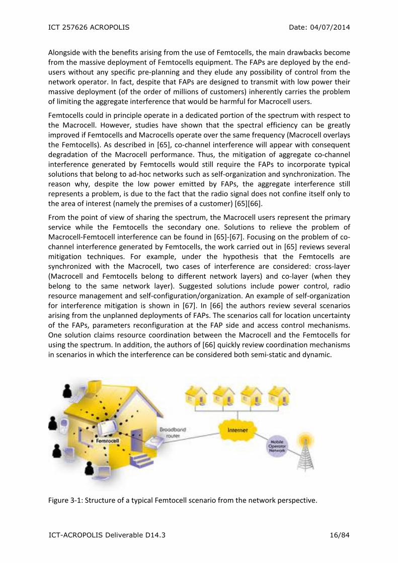
achieve. One answer to such a challenging scenario is constituted by Femtocells (see Figure
3-1).
Femtocells aim to improve the indoor coverage, promising to deliver high enough transfer
rates. The Femtocell is created around the Femto access point (FAP). The FAP uses one of
the typical radio technologies such as UMTS, WiMAx or LTE for the air interface, whilst it
uses a broadband optical fibre or digital subscriber line for the backhaul. The advantages
arising from using Femtocells are multiples, for both operators and users. The users for
example will experience a stronger signal which directly translates into higher reliability and
throughput. For the operators, the use of Femtocells opens to the possibility of scaling down
the unavoidable congestion of network resources from the Macrocell standpoint. This is
simply the consequence of the fact that most of the traffic will be supported over the
Internet Protocol backhaul.
ICT 257626 ACROPOLIS Date: 04/07/2014
ICT-ACROPOLIS Deliverable D14.3 16/84
Alongside with the benefits arising from the use of Femtocells, the main drawbacks become
from the massive deployment of Femtocells equipment. The FAPs are deployed by the end-
users without any specific pre-planning and they elude any possibility of control from the
network operator. In fact, despite that FAPs are designed to transmit with low power their
massive deployment (of the order of millions of customers) inherently carries the problem
of limiting the aggregate interference that would be harmful for Macrocell users.
Femtocells could in principle operate in a dedicated portion of the spectrum with respect to
the Macrocell. However, studies have shown that the spectral efficiency can be greatly
improved if Femtocells and Macrocells operate over the same frequency (Macrocell overlays
the Femtocells). As described in [65], co-channel interference will appear with consequent
degradation of the Macrocell performance. Thus, the mitigation of aggregate co-channel
interference generated by Femtocells would still require the FAPs to incorporate typical
solutions that belong to ad-hoc networks such as self-organization and synchronization. The
reason why, despite the low power emitted by FAPs, the aggregate interference still
represents a problem, is due to the fact that the radio signal does not confine itself only to
the area of interest (namely the premises of a customer) [65][66].
From the point of view of sharing the spectrum, the Macrocell users represent the primary
service while the Femtocells the secondary one. Solutions to relieve the problem of
Macrocell-Femtocell interference can be found in [65]-[67]. Focusing on the problem of co-
channel interference generated by Femtocells, the work carried out in [65] reviews several
mitigation techniques. For example, under the hypothesis that the Femtocells are
synchronized with the Macrocell, two cases of interference are considered: cross-layer
(Macrocell and Femtocells belong to different network layers) and co-layer (when they
belong to the same network layer). Suggested solutions include power control, radio
resource management and self-configuration/organization. An example of self-organization
for interference mitigation is shown in [67]. In [66] the authors review several scenarios
arising from the unplanned deployments of FAPs. The scenarios call for location uncertainty
of the FAPs, parameters reconfiguration at the FAP side and access control mechanisms.
One solution claims resource coordination between the Macrocell and the Femtocells for
using the spectrum. In addition, the authors of [66] quickly review coordination mechanisms
in scenarios in which the interference can be considered both semi-static and dynamic.
Figure 3-1: Structure of a typical Femtocell scenario from the network perspective.

ICT 257626 ACROPOLIS Date: 04/07/2014
ICT-ACROPOLIS Deliverable D14.3 17/84
3.2.2 Scenario2: Opportunistic capacity extension
This scenario depicts a localized region where there is a traffic hot-spot and an opportunistic
network is created in order to route the traffic to non-congested access points. It may also
include cases such as dynamic spectrum management between Macrocells and underlying
micro-, pico- and Femtocells, or 3G traffic offloading towards Wi-Fi.
The generic scenario comprises a congested infrastructure base station (BS), several not-
congested APs (part of the operator’s infrastructure or not), several devices or nodes to
build up the opportunistic network, and one or more terminals that try to connect to the
congested BS.
• In a first step, the type of congestion in a heterogeneous context needs to be
identified, e.g. in case there is a high level of interference due to simultaneous
spectrum access in unlicensed bands, or licensed band systems are overloaded, etc.
• In a second step, the results obtained at the previous step are exploited in order to
eventually reconfigure system parameters (if accessible) and/or use re-routing
strategies in order to route the traffic via uncongested nodes.
Figure 3-2 shows what described above: the incoming device intends to connect to BS1 but
it is instead connected to BS2/Femto-BS/Wi-Fi AP through an opportunistic network.
Figure 3-2: Resolving cases of congested access to the infrastructure – Generic case.
This scenario enables devices to maintain the required level of QoS for a wireless
communication link even when a congestion situation occurs. In particular, the following
two types of congestion situations are considered:
• A system operating in a licensed/unlicensed band is overloaded and cannot
guarantee the provision of the required QoS anymore. In this case, the traffic may be

ICT 257626 ACROPOLIS Date: 04/07/2014
ICT-ACROPOLIS Deliverable D14.3 18/84
re-routed, e.g. based on hot-spots or links via alternative radio access technologies
(RATs) in order to avoid any congested link.
• A system operating in an unlicensed band (e.g., Wi-Fi) or licensed band (such as FAPs
in a randomly deployed dense environment) is experiencing high levels of
interference, since neighbouring APs/BSs are accessing the identical part of the
spectrum. Due to this problem, the link throughput is greatly decreased and a
congestion situation occurs. In this case, a twofold strategy is typically applied: First,
the origin of the interference is identified (which bands are concerned? which Access
Points/Base Stations are concerned?) and the concerned APs/BSs are reconfigured in
order to avoid the congestion situation if possible (e.g., if the concerned system
components belong to a single owner). Typically, it is assumed that the
reconfiguration strategy can be applied to resolve at least part of the problem, while
further measures are needed in order to fully guarantee the required QoS levels. In
particular, re-routing strategies based on opportunistic networks can be adopted to
avoid congested links.
3.2.2.1 Use cases
Three generic use cases that might trigger the creation of an Opportunistic Network (ON)
are presented in this section while more detailed use cases (which may refer to more than
one of these generic scenarios) are analysed in the relative sub-sections.
• Congestion solving: The network should be able to detect congestion situations
when or even before they occur and then try to create one or more opportunistic
networks. These will allow data flows to be re-routed towards not-congested access
points and thus free some resources in affected cells. This use case mainly refers to
users already connected but their QoS starts to degrade due to congestion and or
interference to the Macro-BS and therefore their access needs to be re-routed to a
different BS.
• Congestion access control: This is a generic use case, where a new incoming user
tries to access a congested network access point. An opportunistic network is
created in order to re-route its traffic to a decongested area, thus allowing service
provisioning to a user that otherwise would have been rejected due to lack of
resources.
• Congestion avoidance (Offloading): Whenever possible, the operator will try to
divert traffic towards infrastructure-less access points (e.g., Wi-Fi APs) so that
overlaying cellular (outdoor) network resources are saved. It is a rather proactive
behaviour of the operator so as to avoid potential issues and maintain a balanced
traffic among the Macro-BSs.
3.2.2.2 Congestion solving: the cell edge users case
Figure 3-3 shows the scenario use case where two users are experiencing a very low level of
QoS because
• the neighbouring Macro-BS are heavily loaded,
• the concerned user equipment (UEs) are close to the cell-edge.

ICT 257626 ACROPOLIS Date: 04/07/2014
ICT-ACROPOLIS Deliverable D14.3 19/84
Since the demand of radio resources that are required for delivering high data rate services
to those cell-edge users could exceed the capability of the network, the concerned devices
typically will not be able to achieve their target QoS.
Figure 3-3: Resolving cases of congested access to the infrastructure (congested Macro-BS)
Neighbouring RATs (in this example, “RAT B”, “RAT C” and “RAT D”3) are used in order to
set-up an opportunistic network and enable high data-rate/high QoS services for the
concerned UEs (in particular to those positioned at cell edges). It should be noted that the
main focus is on Femtocells able to cover the same service region, and/or on macro BSs
(which may be covering neighbouring service area regions; in this case it can be assumed
that the traffic is routed to them through Ad-hoc networks).
In the context of Macrocell/Femtocell management (when RAT B/C/D are Femtocells),
resolving congested access to a Macrocell can be done by allocating spectrum to Femtocells
in the area: the Macrocell can decide the most efficient configuration (in terms of spectrum
and power) of the Femtocells with the following objectives:
• offload a number of terminals to the Femtocells so that the load on the Macro-
cell does not exceed a threshold;
• minimize Femtocells to Macrocell interferences when both operate over the
same band.
It is worth noticing that these two objectives are conflicting: having in fact a high number of
terminals capable of connecting to the Femtocell means increasing the power of the FAP,
thus causing interference to the Macrocell; minimizing the interferences by reducing the
power allocated to the Femtocell means reducing the coverage of the FAP and so the
number of terminals that can are served. In this scenario, the Femtocell parameters are
adjusted depending on the capability to create opportunistic networks that allow terminals
connecting to the Femtocell to relay data from/to neighbouring terminals that are not in
coverage of the Femtocell itself.
3 The new RATs B, C and D either represent Femto-BS for Resource Management between Femto/Macro-BS or
RATs which have not been designed in an integrated framework (such as various Wi-Fi flavours, WiMAX, etc.)
ICT 257626 ACROPOLIS Date: 04/07/2014
ICT-ACROPOLIS Deliverable D14.3 20/84
3.2.2.3 Congestion solving/avoidance: Macrocell/Femtocell management case
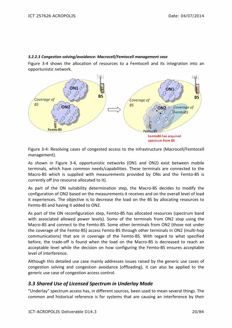
Figure 3-4 shows the allocation of resources to a Femtocell and its integration into an
opportunistic network.
Figure 3-4: Resolving cases of congested access to the infrastructure (Macrocell/Femtocell
management).
As shown in Figure 3-4, opportunistic networks (ON1 and ON2) exist between mobile
terminals, which have common needs/capabilities. These terminals are connected to the
Macro-BS which is supplied with measurements provided by ONs and the Femto-BS is
currently off (no resource allocated to it).
As part of the ON suitability determination step, the Macro-BS decides to modify the
configuration of ON2 based on the measurements it receives and on the overall level of load
it experiences. The objective is to decrease the load on the BS by allocating resources to
Femto-BS and having it added to ON2.
As part of the ON reconfiguration step, Femto-BS has allocated resources (spectrum band
with associated allowed power levels). Some of the terminals from ON2 stop using the
Macro-BS and connect to the Femto-BS. Some other terminals from ON2 (those not under
the coverage of the Femto-BS) access Femto-BS through other terminals in ON2 (multi-hop
communications) that are in coverage of the Femto-BS. With regard to what specified
before, the trade-off is found when the load on the Macro-BS is decreased to reach an
acceptable level while the decision on how configuring the Femto-BS ensures acceptable
level of interference.
Although this detailed use case mainly addresses issues raised by the generic use cases of
congestion solving and congestion avoidance (offloading), it can also be applied to the
generic use case of congestion access control.
3.3 Shared Use of Licensed Spectrum in Underlay Mode
“Underlay” spectrum access has, in different sources, been used to mean several things. The
common and historical reference is for systems that are causing an interference by their

ICT 257626 ACROPOLIS Date: 04/07/2014
ICT-ACROPOLIS Deliverable D14.3 21/84
transmissions that is below the noise power spectral density at the primary, typically
through transmitting with a very wide bandwidth, for example, such as through impulses
transmissions. More recently, underlay spectrum access has often also been used to refer to
systems that transmit while causing less than a given threshold of interference power or
interference power spectral density at the primary receiver. This section briefly overviews
both such cases.
3.3.1 Ultra-Wide Band
UWB technology, which is a radar technology, represents probably the first historical
attempt to enable improved forms of spectrum access (i.e., underlay communications). In
recent years, UWB has attracted great interest of academia and industry due to the unique
characteristics of the signal, which makes it appealing for a large variety of civil applications:
short-range communications, Internet, localization at centimeter-level accuracy, high-
resolution ground-penetrating radar, through-wall imaging, precision navigation and asset
tracking, just to name a few.
A signal is defined to be UWB according to the two following definitions: for a central
frequency less than 2.5 GHz its fractional bandwidth (Wf) has to be greater than 20%, whilst
above 2.5 GHz its bandwidth (W) has to be at least 500 MHz [17]-[19][68]. The fractional
bandwidth of the signal is defined as: Wf=2(fh-fl)/fh+fl, where fh and fl stands for the high and
low cutoff frequencies measured at either -3 dB or -10 dB, depending on the definition.
Already in 2002 the FCC in the USA regulated the use of UWB handheld devices in the huge
frequency range 3.1-10.6 GHz. The FCC regulated emission levels of UWB devices to -41.3
dBm/MHz to avoid harmful interference toward systems already existing (e.g., the Global
Navigation System - GPS).
The large bandwidth, the simplicity of the transmitted signal that consists of the
transmission of a train of baseband nanosecond pulses having a very low level of emitted
power (in theory below the noise floor) made UWB attractive for enabling the applications
mentioned above. Over time, UWB can be seen as the attempt to bring to the extreme the
concepts of a spread spectrum system and the first in its kind to make more efficient use of
the wireless spectrum. Mainly two techniques are available to generate an UWB signal. The
first approach consists of generating nanosecond pulses and it constitutes the basis for
time-hopping UWB systems [69]. The second consist of bonding together frequency bands
in order to produce an ultra-wide bandwidth. This last approach was used in [70] and in the
literature is referred to as multi-band UWB.
More recently, UWB systems have been classified within the larger group of dynamic
spectrum access techniques and in particular the ones that are referred to as underlay
communications [60]. In this case, secondary users are forced to transmit with extremely
low power levels (below the noise floor) such that the primary user is unaffected by
secondary transmissions. With respect to the taxonomy defined in [60], UWB
communications break the secondary-usage barrier and the exclusive-usage barrier that are
nowadays in force in the allocation of spectrum for wireless services. However, peaks of
spectral lines caused by specific modulation schemes reveal that UWB is not totally capable
to coexist with other wireless systems without causing harmful interference.

ICT 257626 ACROPOLIS Date: 04/07/2014
ICT-ACROPOLIS Deliverable D14.3 22/84
The natural solution that aims to improve the coexistence between secondary UWB devices
and primary services goes under the name of detect and avoid (DAA) techniques [71]-[76].
For example, as pointed out in [71], UWB devices might not be able to coexist with other
wireless systems despite the restrictive power emission regulations. A study on the
coexistence between UWB and other systems like UMTS, GPS and fixed wireless systems is
shown in [72]. In this study, UWB devices are limited to indoors (that is the main application
of UWB systems) while the victim systems could be either inside or outside the building
(that is intended as a commercial/industrial building). Secondary devices make use of the
time-hopping UWB signaling scheme.
Literally, DAA means that UWB devices are capable of sensing the power within the band of
the victim system and whenever the threshold set for reception is exceeded, UWB devices
have to modify their transmission parameters in order to avoid interfering. UWB devices
perform these operations on a non-cooperative basis (this is at least the most common way
of approaching the problem) with respect to the primary system, which ignores the
presence of UWB transmitters. The main limitation of this approach is the need to sense
signals as low as the sensitivity of the victim receiver (well below -100 dBm). Therefore,
sophisticated measurement instruments are required, which increase the cost of the UWB
devices.
In [73] and [74], DAA techniques for UWB devices (also these studies are tailored for time-
hopping UWB) potentially interfering with UMTS and WiMAX systems are devised,
respectively. The key idea in [72] and [73] is to detect the uplink primary transmission and
accordingly adjust transmit power and data rate to reduce/avoid interfering with the victim
system. Furthermore, the outcome of the DAA could even consist of suspending completely
the transmissions of the secondary devices for the time necessary by the primary UEs to
complete network association. A performance metric that could be used in these cases is
given by the fraction of time that a period of primary user activity is jammed by UWB
devices. In the mentioned papers, the DAA includes two sub-phases: detection and
transmission for the purposes mentioned already. For the sake of completeness, as an
example, the cooperative approach and the advantages for the UWB system are shown [75].
In [76] DAA technique adapted to the specific scenario of a UWB-WiMAX system is
investigated. The study is based on the concept of low-duty-cycle and it is applied in the
frequency band 3.1-4.8 GHz. The devices this time are using multi-band UWB transmission
technology. The study shown in the paper relies also on European regulations for the power
emissions of UWB devices in indoors [77]. In essence, the coexistence mechanism consists
of defining different thresholds for signal detection and different transmit power levels
based on the proximity of a UWB device with respect to the WiMAX receiver. In particular,
three zones are identified. In the first zone UWB devices can transmit with a power spectral
density of -41.3 dBm and use a threshold for detection of -61 dBm. In the second zone the
UWB devices use a threshold of -38 dBm and a power spectral density of -65 dBm/MHz. In
the last zone (which implies close proximity to the WiMAX receiver) the emitted power
spectral density is set to -80 dBm/MHz for a distance below 36 cm, whereas the threshold
for the detection of the signal remains the same.

ICT 257626 ACROPOLIS Date: 04/07/2014
ICT-ACROPOLIS Deliverable D14.3 23/84
3.3.2 Interference Threshold
This approach assumes that a known threshold for allowable interference at the primary
receiver is enforced or otherwise assumed, whereby the secondary will transmit up to a
power level that would cause no more than that interference threshold. A key challenge
with such an approach is that, typically, neither the positions, nor propagation/channel
characteristics, of/toward the primary receiver from the secondary transmitter are typically
known. Correspondingly, it is very difficult if not impossible to ascertain the allowable upper
transmit power level of the secondary, especially in dynamic scenarios involving motion of
the primary receivers and/or the secondary transmitters. That is not to say, however, that
such an approach cannot be useful. If well-known “reference scenarios” for the positions of
the primary receivers are defined, such as for TV White Spaces whereby the types of
primary receivers, their positions (e.g., locations on/within a building), and motilities (or lack
thereof) can be defined with a relatively high certainty, the secondary transmit power limits
can be ascertained with a higher confidence level of not causing more than the interference
threshold. Such assumptions apply for regulatory modeling of interference, and indeed can
be seen in some sense as related to interference threshold models.
Aside from such cases, the most prominent example of such interference limit models is the
“Interference Temperature” concept as proposed by the FCC.
3.3.2.1 Interference Temperature Model
The FCC introduced the concept of interference temperature (IT) in 2003, for “quantifying
and managing interference” [62]. As described already elsewhere in this document, a CR
networks may coexist with the primary user either on a non-interference basis or on
interference-tolerant basis. In the first case, as mentioned, the CR devices are allowed to
operate only on those bands that are not used by the primary user (i.e., White Spaces). In
the second case instead, CR devices can access the same frequency band of the primary user
as long as the aggregate interference power falls below a certain threshold. The case in
which CR devices can operate simultaneously with the primary transmission is commonly
known as the interference temperature case.
When analysing interference-limited CR systems, it is necessary to specify the IT constraint
for the primary receiver along with the specification of the transmit power constraint of the
CR transmitters. As such, this is the problem of optimizing a system subject to multiple
constraints. The limits of interference temperature limited single-antenna CR systems was
analysed in [78] in the presence of fading. The capacity and power constrained problem
arising in such single-antenna system with fading was investigated in [79]. The work done
instead in [80] and [81] investigates interference temperature limited CR systems in multiple
input single output (MISO) and multiple input multiple output (MIMO) cases, respectively.
It is important mentioning that the FCC recently dropped the concept of interference
temperature declaring it as not a workable concept [82]. This was due to the observation
made by several industries that the concept of interference temperature, if adopted, would
have resulted in an increased interference in the frequency bands where it would have been
used.
ICT 257626 ACROPOLIS Date: 04/07/2014
ICT-ACROPOLIS Deliverable D14.3 24/84
3.4 Spectrum Commons and Related Models: Interference among Secondary
Systems
3.4.1 In Opportunistic Secondary Spectrum Access Scenarios: TV White Spaces
Interference may occur among secondary systems in cases of secondary spectrum usage, for
instance among the secondary systems using UHF TV White Space frequency bands. In the
particular case of TV White Space, numerous secondary systems are either defined or being
defined for operation in TV White Space, including ECMA-392 [83], IEEE 802.22 [84], IEEE
802.11af [85], IEEE 802.15.4m [86], IEEE 1900.7 [87], among others. Considering that in
many locations the number of channels available for TV White Space access will be very
limited, the interference that these systems cause on each other could quickly lead to a
situation where the available White Spaces become unusable for secondary access.
In the case of TV White Space, a number of opportunities exist to do things better than in
the case of ISM and other unlicensed bands. In such a case, there is already a database
entity that, especially for Ofcom and CEPT other proposed rules [88] [89][90], would be able
to not only manage secondary access to protect the primary, but also potentially could
operate outside of its proposed purpose in managing the interference powers among
secondary systems. Such as case, from the regulator’s point of view, is nevertheless out of
scope of consideration, and could also be seen as medalling in fair competition between
users. There are scenarios, however, such as in ASA and related concepts, where such
management could be applicable. If a spectrum owner were to provide its own database to
allow opportunistic access of its spectrum, e.g., for a fee, then that spectrum owner could
validly manage the powers among the secondary systems to avoid interference, as well as
potentially implementing far more complex management concepts than just transmission
power adaptation.
Aside from such possibilities, interference among secondary systems is subject to many of
the same considerations and challenges as interference in unlicensed bands. It is noted that,
however, there are different sets of equipment operating in White Space compared with
unlicensed bands, due to various factors such as maturity of technology, contributions and
spectrum opportunities and the desire to develop systems that can take advantage of
opportunities better, as might become available in White Space, and tougher regulatory
rules and challenges such as transmission masks, among others.
3.4.2 In Conventional Unlicensed Spectrum: ISM bands
The case of spectrum sharing and interference in conventional unlicensed spectrum like for
example ISM (2.4 GHz) and U-NII (5 GHz) bands is referred as uncontrolled commons or
open spectrum access [60]. In this scenario any one can operate as many devices as he want
and no specific rules have been defined to avoid or reduce interference. Regulation bodies
like FCC or ECC only require that a certain maximum peak power is not exceeded. Therefore
several devices belonging to independent systems can be active at the same time in the
same portion of spectrum. As previously indicated, if each single system is only trying to
maximizing its own performance without considering external factors the so called “tragedy
of commons” is expected to happen [91]. For this reason, although standards are rapidly
getting more and more performing (e.g: IEEE 802.11n) creation of reliable, revenue
generating services in unlicensed spectrum continues to be less than viable due to this
weakness. An additional limitation is represented by the multitude of different systems and
ICT 257626 ACROPOLIS Date: 04/07/2014
ICT-ACROPOLIS Deliverable D14.3 25/84
standards operating in the same spectrum band. This make difficult to define techniques to
mitigate possible interference scenarios. For this reason many efforts to avoid “the tragedy
of commons” didn’t encounter much resonance in the industry. In [59] one of these efforts
referred as “Managed Commons” has been presented together with the main desirable
characteristics for a good commons management protocol.
3.4.3 In Unlicensed bands: Use of Opportunistic Wi-Fi Networks for Resolving Interference
among different RATs
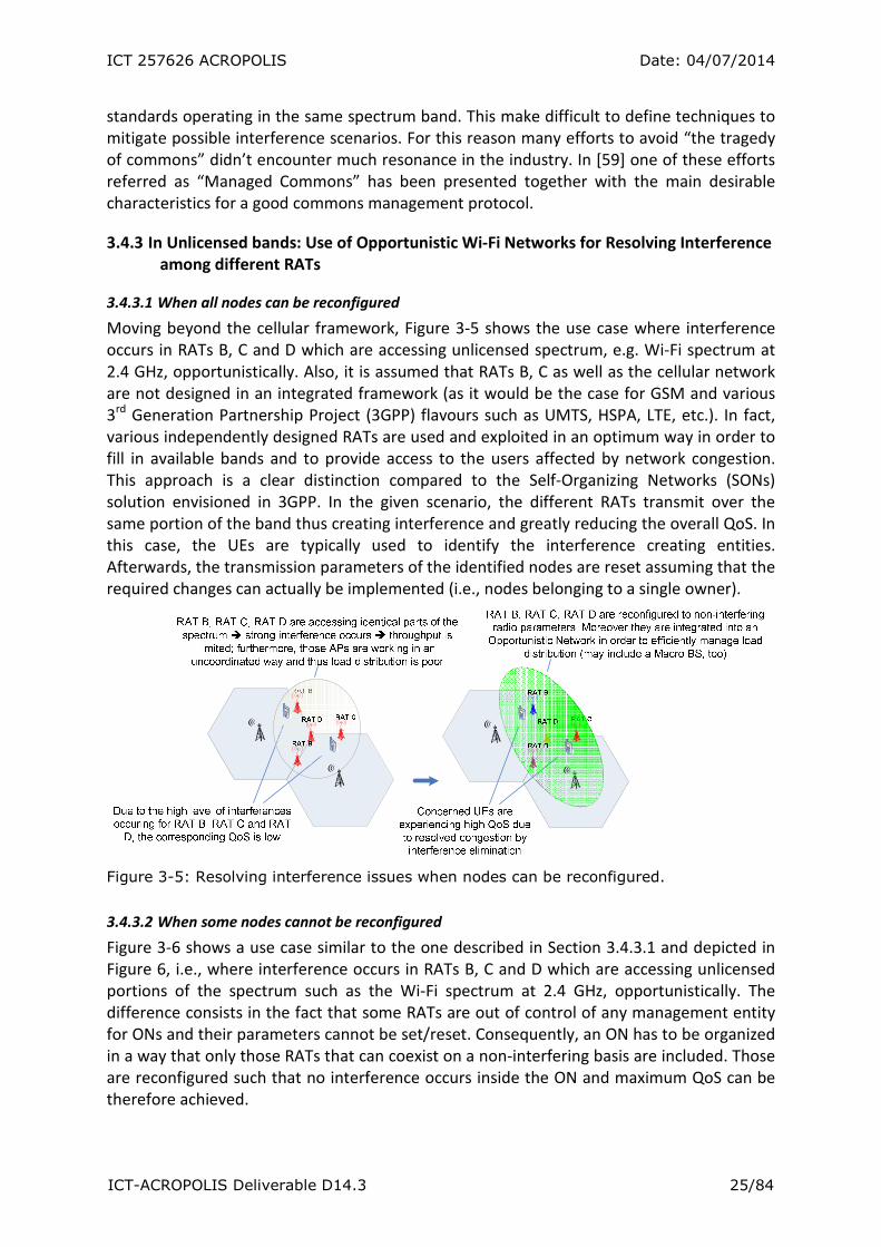
3.4.3.1 When all nodes can be reconfigured
Moving beyond the cellular framework, Figure 3-5 shows the use case where interference
occurs in RATs B, C and D which are accessing unlicensed spectrum, e.g. Wi-Fi spectrum at
2.4 GHz, opportunistically. Also, it is assumed that RATs B, C as well as the cellular network
are not designed in an integrated framework (as it would be the case for GSM and various
3rd
Generation Partnership Project (3GPP) flavours such as UMTS, HSPA, LTE, etc.). In fact,
various independently designed RATs are used and exploited in an optimum way in order to
fill in available bands and to provide access to the users affected by network congestion.
This approach is a clear distinction compared to the Self-Organizing Networks (SONs)
solution envisioned in 3GPP. In the given scenario, the different RATs transmit over the
same portion of the band thus creating interference and greatly reducing the overall QoS. In
this case, the UEs are typically used to identify the interference creating entities.
Afterwards, the transmission parameters of the identified nodes are reset assuming that the
required changes can actually be implemented (i.e., nodes belonging to a single owner).
Figure 3-5: Resolving interference issues when nodes can be reconfigured.
3.4.3.2 When some nodes cannot be reconfigured
Figure 3-6 shows a use case similar to the one described in Section 3.4.3.1 and depicted in
Figure 6, i.e., where interference occurs in RATs B, C and D which are accessing unlicensed
portions of the spectrum such as the Wi-Fi spectrum at 2.4 GHz, opportunistically. The
difference consists in the fact that some RATs are out of control of any management entity
for ONs and their parameters cannot be set/reset. Consequently, an ON has to be organized
in a way that only those RATs that can coexist on a non-interfering basis are included. Those
are reconfigured such that no interference occurs inside the ON and maximum QoS can be
therefore achieved.

ICT 257626 ACROPOLIS Date: 04/07/2014
ICT-ACROPOLIS Deliverable D14.3 26/84
Figure 3-6: Resolving interference issues when some nodes cannot be reconfigured.
ICT 257626 ACROPOLIS Date: 04/07/2014
ICT-ACROPOLIS Deliverable D14.3 27/84
4. Models of Wireless Interference
The aim of this section is to present a thorough though succinct overview of some
fundamental aspects connected with the modelling of the aggregate interference in wireless
systems. This quite basic approach will be at the end extended to the specific case of
cognitive radios. Referring to the generic d space and a point y in it, the aggregate
interference measured at the location y can be written as follows
∑Τ∈
−=x
xx xylhPyI )( , (1)
whereΤ denotes the set of active transmitters, Px is the transmitted power of node x, hx is
the (power) channel fading coefficient for the link between x and y and xyl − denotes the
path-loss due to the distance affecting the link between the two nodes. In the remainder of
this document the analysis of the interference is clearly important for interference-limited
networks such as cognitive radio systems.
Aggregate interference plays a major role in many aspects of management and optimization
of wireless networks. In essence, aggregate interference in the shared wireless channel has
a number of implications on network performance. One of the main working assumptions in
wireless communications, made from the system standpoint, is to determine an exclusion
region around the transmitter-receiver pair in order to obtain a communication free from
interference [92][93]. This is the typical way of proceeding in many papers dealing with MAC
protocols, for example. These papers try, to some extent, to enable access to the wireless
channel in such a way to reduce (or minimize) the probability that two or more packets
collide at the same receiver, thus causing multi user interference (MUI).
Despite all the attempts to minimize the aggregate interference between communication
systems sharing the same frequency band at the same time and location, the problem still
exists. Depending on the radio technology used, narrowband or ultra wideband, the type
environment where the network has to operate (urban or countryside), performance may
vary quite dramatically. In a realistic environment, the location of the wireless devices with
respect to the receiver, the time of arrival of the received packets and the different levels of
received power affect the performance of a wireless link. All these effects fall in the set of
near-far effects. Therefore, in realistic scenarios where packets suffer from collisions, if a
packet is received correctly, although in principle it collided with other concurrent
transmissions, is said to capture the intended receiver. This effect is known in the literature
of MAC protocols as the capture effect. Often the capture is defined as follows
+> ∑
≠ijWjjii NPgPPg 0,0, ϑ ,
(2)
where Pi is the transmit power of the ith terminal4, while the sum represents the aggregate
interference power, NW is the additive white Gaussian noise with two-sided power spectral
4 When power control is applied it holds that Pi≠ Pj.

ICT 257626 ACROPOLIS Date: 04/07/2014
ICT-ACROPOLIS Deliverable D14.3 28/84
density N0/2 and Pθ is the threshold (referred to as capture power ratio) for accepting the
packet of node i and it typically depends on the application. The terms gi,0 and gj,0 denote
the power gains introduced by the channel in the test link and in the jth interfering link,
respectively. Typically, they incorporate random propagation effects such as power-law
decay, fading and shadowing. The power-law decay can be expressed as r-2b
, where
parameter b is the typical path-loss exponent that equals 1 in free space. The term r-2b
is
itself a random variable (r.v.) that follows some statistical distribution. The work done in
[94] shows that, under the assumptions that fading, shadowing and locations of individual
transmitters are independent, for a large number of stations (theoretically going to infinity)
and under very broad conditions, the capture ratio in (2) depends only on the capture
power ratio γ and on the path-loss exponent b.
4.1 Validity of Gaussian modelling for the interference
The capture model has been successfully applied to model realistic performance of packet
switched radio networks under various transmission schemes and propagation effects. For
example, capture was used to model the performance of mobile spread spectrum systems
and more in general the basic but important case of a slotted Aloha (S-Aloha) network.
Models have been developed to account for different modulation schemes, fading effects
and shadowing. In all cases, modelling of the interference assume a central role. In brief, the
capture model has bridged the algorithmic approach usually taken at levels of the OSI model
higher than the physical layer and typical propagation effects affecting radio signals. In most
or even all the studies, modelling the interference as the result of the superposition of
individual and independent radio transmitters displaced in space has represented one of the
primarily tasks, though very challenging. Modelling the aggregate interference as a Gaussian
process is appealing due to its simplicity and direct use of the central Limit Theorem (CLT) in
the presence of a large number of interferers. Despite this model has been used, soon it
received criticisms as it does not account for the spatial distribution of the nodes.
In [95] and [96] the spatial capacity of a multihop S-Aloha network and the benefit owed to
spatial reuse have been investigated, respectively. Both papers model the distribution of
nodes in space as a two dimensional Poisson Point Process (PPP) as show in (3), with λ the
intensity function of the point process and ||A|| denotes the Lebesgue measure of set A. In
particular, [95] models the throughput of the multihop network as the result of a spatial
process in which packets from the devices are received correctly when no other nodes
transmit within the same region of space. In [96] it is shown how spatial reuse can be
introduced in the study of the performance of a multihop network when nodes are at least
three hops apart. Moreover, network topologies that allow spatial reuse are discussed. In
particular, [96] shows a previous result in which nodes are arranged on the vertices of
equilateral triangles repeated over the network topology. Assuming that each node has a
range of r=1 meters, the average distance between nodes is surprisingly equal to 2.
( ) A
k
ek
AinnodeskP
λλ −=Α!
. (3)
When tackling the problem of studying the performance multihop network from a
geometrical perspective, one interesting result can be obtained by computing the average
distance among nodes. Referring to Figure 4-1, nodes are uniformly deployed inside the
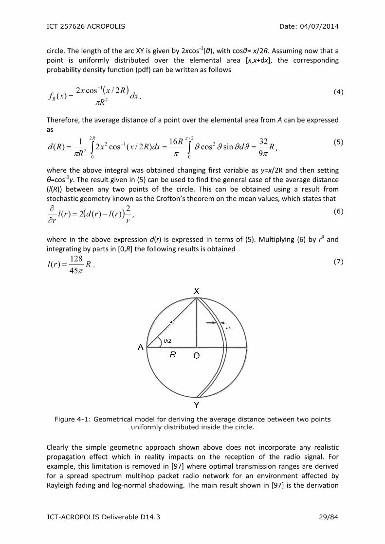
ICT 257626 ACROPOLIS Date: 04/07/2014
ICT-ACROPOLIS Deliverable D14.3 29/84
circle. The length of the arc XY is given by 2xcos-1
(θ), with cosθ= x/2R. Assuming now that a
point is uniformly distributed over the elemental area [x,x+dx], the corresponding
probability density function (pdf) can be written as follows
( )dx
R
RxxxfR 2
1 2/cos2)(
π
−
= . (4)
Therefore, the average distance of a point over the elemental area from A can be expressed
as
RdR
dxRxxR
Rd
R
∫∫ === −2/
0
21
2
0
2
2 9
32sincos
16)2/(cos2
1)(
π
πϑϑϑϑ
ππ,
(5)
where the above integral was obtained changing first variable as y=x/2R and then setting
θ=cos-1
y. The result given in (5) can be used to find the general case of the average distance
(l(R)) between any two points of the circle. This can be obtained using a result from
stochastic geometry known as the Crofton’s theorem on the mean values, which states that
( )r
rlrdrlr
2)()(2)( −=
∂
∂,
(6)
where in the above expression d(r) is expressed in terms of (5). Multiplying (6) by r4 and
integrating by parts in [0,R] the following results is obtained
Rrlπ45
128)( = .
(7)
Figure 4-1: Geometrical model for deriving the average distance between two points
uniformly distributed inside the circle.
Clearly the simple geometric approach shown above does not incorporate any realistic
propagation effect which in reality impacts on the reception of the radio signal. For
example, this limitation is removed in [97] where optimal transmission ranges are derived
for a spread spectrum multihop packet radio network for an environment affected by
Rayleigh fading and log-normal shadowing. The main result shown in [97] is the derivation

ICT 257626 ACROPOLIS Date: 04/07/2014
ICT-ACROPOLIS Deliverable D14.3 30/84
of the transmission range of a device so that, on average, it has the optimum number of
neighbours. Furthermore, this work enhances the one made in [98] where optimum
transmission ranges were found for a packet switched radio network but with simpler
channel propagation effects.
As mentioned already above, the assumption of the Poisson distribution of the devices over
space and the Gaussian modelling of the distribution of the aggregate interference power
provided already a good insight of the network behaviour. This has represented a
fundamental step that bridged together the systemic approach with the physics of the radio
signal propagation. Examples aligned with this view can be found in [99]-[101]. However,
these papers started debating the validity of the Gaussian assumption for modelling the
interference power distribution. For instance, one hit that unhinged this conjecture came
out when studying the performance of impulse radio UWB systems. In fact, the work done
in [102] and [103] showed that the Gaussian approximation is too poor to predict accurately
the performance.
The tool of stochastic geometry provides an excellent mean to devise the performance of
packet switched radio networks in which devices generate harmful interference affecting
each other’s behaviour. The core contribution of this approach consists of modelling the
nodes of a wireless network as a point process (PP). This approach was already pursued in
the seminal papers [37][38] and [98] just to name a few. More recently this modelling
approach have been rediscovered and adapted to more recent scenarios, radio technologies
and networks. This is evident from [16][23]-[27][54][104]-[106]. In particular, [105] and
[106] challenge the validity of the spatial Poisson model for the sake of obtaining an
accurate prediction of the network behaviour.
Accordingly to such recent trend in communications, the next sections are devoted to
review how stochastic geometry is helpful for modelling the behaviour of a wireless network
where the aggregate interference assumes the key role.
4.2 Stable distributions
Historically, modelling the distribution of the aggregate interference power has witnessed
important progresses especially with the two seminal papers [37] and [38]. In particular,
both papers subsume that the distribution of the aggregate interference power generated
by a Poisson field of interferers belongs to the family of stable distributions. Stable
distributions belong to the family of heavy tail distributions. A typical example of one-side
heavy tail distribution is the Pareto distribution. Two-side heavy tail distributions are the
Cauchy and Lévy distributions. A probability distribution is considered heavy-tailed when the
tails of such distribution are not exponentially bounded or, in other words, the tails are
heavier than the exponential distribution.
This section is concentrated on the family of stable distributions, which belong to the two-
tail distributions. Stable distributions can be considered as a result of the generalization of
the CLT dealing with the sum of independent and identically distributed (iid) r.vs. whose
variance is not finite. Thus, the Normal Gaussian distribution can be seen as particular case
of stable distributions. In general, there is no closed form expression for the cumulative
distribution function (CDF) and the pdf of stable distributions except for the Cauchy and
Lévy distributions which represent special cases.
ICT 257626 ACROPOLIS Date: 04/07/2014
ICT-ACROPOLIS Deliverable D14.3 31/84
A univariate Cauchy distributed r.v. x is characterized by the following pdf and CF5:
( )ωγωδωφ
γδ
πγ
−=
∞<<∞−
−+
=
i
xx
xf
exp)(
,
1
1)(
2
,
(8)
where 1−=i is the imaginary unit. On the other hand, a Lévy distributed r.v. X is
characterized by the following pdf and CF:
( )( )γωωδωφ
δδ
γδπ
γ
ii
xxx
xf
2exp)(
,)(2
exp1
2)(
2/3
−−=
∞<≤
−−
−=
,
(9)
At this point it can be given the first formal definition of a univariate stable distributed r.v. X.
The following discussion on stable distributions will rely on [107] for notation and the
definition of related concepts.
Definition 1: A r.v. X is stable or stable in the broad sense if for X1 and X2 independent
copies of X and any positive constants k1 and k2 and positive numbers c, d ϵ the following
equality holds
dcXXkXkd
+=+ 2211 , (10)
where the equality above holds in distribution. The r.v. is strictly stable or stable in the
narrow sense if (10) holds with d=0 for ant value assigned to k1 and k2. A r.v. X is symmetric
stable if it is stable and symmetrically distributed around zero, that is X=-X in distribution. In
other words, (10) states that the shape of X is unchanged under addition operation.
Definition 2: A r.v. x is stable distributed S(α,β,γ,δ,1)6 if and only if it exists a r.v. Z having
the following CF
( )
=
+
+−
≠
+
−−
=
1 )log()(2
1exp
1 2
tan)(1exp
exp
αδωωπ
βω
αδωπα
ωβω
ω
α
iwsigni
isigni
ziE ,
(11)
where the log() stands for the natural logarithm and in distribution it holds that
5 The CF of a r.v. x is defined as Eexp(iωx).
6 The notation S(α,β,γ,δ,1) will be abbreviated in S(α,β,γ,δ) in the remainder of this text.

ICT 257626 ACROPOLIS Date: 04/07/2014
ICT-ACROPOLIS Deliverable D14.3 32/84
=
++
≠+
=1 log
2
1
αγγπ
βδγ
αδγ
z
z
xd
Therefore, in this case X has the following CF:
( )
=
+
+−
≠
+
−−
=
1 )log()(2
1exp
1 2
tan)(1exp
exp
αδπ
βγ
αδπα
βγ
ω
αα
wiwwsigniw
wiwsigniw
xiE ,
(12)
The four parameters which are entries of the stable distribution are defined as follows
- α: index of stability or characteristic exponent defined in (0,2]
- β: skewness defined in [-1,1]
- γ: scale parameter or dispersion defined in [0,∞ )
- δ: location parameter define for all .
It is important to remark few facts related to the stable distribution: parameter γ must not
be confused with the standard deviation and parameter δ must be confused with the mean.
In addition, since α and β determine the shape of the distribution they can be interpreted as
shape parameters.
At this point it is clear that the Gaussian, Cauchy and Lévy distributions can be seen as
special cases of the family of stable laws. Thus, the Gaussian distribution can be seen as
S(2,0,γ,δ) with γ properly set with respect to the standard deviation. The Cauchy
distribution is S(1,0,γ,δ) and the Lévy distribution is S(1/2,1,γ, δ). When γ =1 and δ =0 the
stable distribution is said standardized. On the other hand, β =0 define the important case
of the family of symmetric stable distributions (SαS). For symmetric stable distribution the
CF reduces to
( )αωγωφ −= exp)( (13)
Some general properties of the stable distributions are:
1. All (non-degenerate7) stable distributions are continuous distributions with an
infinitely differentiable density.
2. Reflection property: for any α and β, let the r.v. Z~S(α,β) and ),(),( βαβα ZZd
−=− .
Therefore, the density and distribution function of Z satisfy f(x|α,β)=f(-x|α,-β) and
F(x|α,β)=1-F(-x|α,-β).
3. Scaling property: Let the r.v. X~S(α,β) with 1≠α and let k1 be a positive real
constant. Then, k1X~ S(α,sign(k1)β, |k1|α
γ)
7 A degenerate distribution is the probability of a r.v. which takes only a single value.

ICT 257626 ACROPOLIS Date: 04/07/2014
ICT-ACROPOLIS Deliverable D14.3 33/84
4. Decomposition property: if the r.v. X~S(α,0,γ) then it can be decomposed as
ZVX = , where in this case the r.v. Z is Gaussian Z~N(0,2γ2/ α
) and V~S(α/2,1,
cos(π α/2)).
Stable distributions will assume an important role when modelling the distribution of the
aggregate interference power generated by an infinite number of nodes distributed over
space according to a PPP. Below are shown some plots for stable distributions and different
values of the four defining parameters discussed above.
-4 -3 -2 -1 0 1 2 3 40
0.1
0.2
0.3
0.4
0.5
0.6
0.7
x
Pro
babili
ty d
ensity f
un
ction (
pdf)
Stable distributions - β=0, γ=1, δ=0
α=0.5
α=1
α=1.5
α=2
Figure 4-2: Probability density function of a symmetric stable distributed r.v.
-4 -3 -2 -1 0 1 2 3 40
0.1
0.2
0.3
0.4
0.5
0.6
0.7
0.8
0.9
1
x
Cum
ula
tive
dis
trib
utio
n f
unction (
CD
F)
Stable distributions - β=0, γ=1, δ=0
α=0.5
α=1
α=1.5
α=2
Figure 4-3: Cumulative distribution function of a symmetric stable distributed r.v.

ICT 257626 ACROPOLIS Date: 04/07/2014
ICT-ACROPOLIS Deliverable D14.3 34/84
-4 -3 -2 -1 0 1 2 3 40
0.1
0.2
0.3
0.4
0.5
0.6
0.7
x
Pro
babili
ty d
ensity f
un
ction (
pdf)
Stable distributions - α=0.5, γ=1, δ=0
β=0
β=0.25
β=0.5
β=0.75
β=1
Figure 4-4: Probability density function of a skewed stable distributed r.v.
-4 -3 -2 -1 0 1 2 30
0.1
0.2
0.3
0.4
0.5
0.6
0.7
0.8
0.9
x
Cum
ula
tive
dis
trib
utio
n f
unction (
CD
F)
Stable distributions - α=0.5, γ=1, δ=0
β=0
β=0.25
β=0.5
β=0.75
β=1
Figure 4-5: Cumulative distribution function of skewed stable distributed r.v.
4.2.1 Useful facts
An important function that will be often used to compute the distribution of the aggregate
interference is the Gamma function, which is defined as
( ) ∫∞
−−=Γ0
1 dtetz tz
a , (14)
considering that ( ) )!1( −=Γ zz if z assumes only integer values. Another function that will
be used is the standard Q-function, whose expression is the following
dxexQx
x∫∞ −= 2/2
2
1)(
π.
(15)

ICT 257626 ACROPOLIS Date: 04/07/2014
ICT-ACROPOLIS Deliverable D14.3 35/84
Furthermore, the following two integrals will be used during the following calculations
( ) ( ) ( ) α
α απαα
zdtt
zt 2/cos1cos1
0
1
−Γ=
−∫∞
+ , (16)
( ) ( ) ( ) α
α απααφ
ZEdtt
t 2/cos11
0
1
0 −Γ=
−∫∞
+ (17)
Where φ(t) is the CF of the aggregate interference. To solve the last integral it was used the
following property of the Gamma function Γ(1-α)= Γ(2-α)/(1- α).
Channel propagation effects such as fading and shadowing greatly affect the reception of a
radio signal and so reduce the throughput of a communication link. For the specific case of
Rayleigh fading, the general result prescribes computing the parameters of the stable
distribution that models the aggregate interfering process
( )2/12 2/ ααα +Γ=EZ (18)
For Nakagami-m fading instead
( )( )
2/2/
αα α
Κ
Γ+Γ
=mm
mEZ m
, (19)
Where 2EZm =Κ . Finally for log-normal shadowing with variance σ2
instead
= 22
2
1exp σααEZ
(20)
As it shall be seen later, the multivariate LePage series representation will provide us with
an important tool to characterize the aggregate interference under the assumption of PPP.
The definition of a spherically symmetric (SS) r.v. (respectively random vector) is provided in
Definition A5 in Section 0.
Definition 1 (LePage series):
Let us consider a real random vector Y=[Y1,Y2, ….,Yd] with Yi SS α-stable r.vs. Thus, the vector
Y is SS α-stable if the joint CF is of the following form
( )
−== ∑
=
2/
1
2
1 exp,...,)(
α
γφφd
i
id tttt . (21)
Theorem 1: Let τi denote the arrivals of a Poisson process and let Xi be SS iid vectors in d,
independent on τi, with E|Xi|α<∞ , then Y can be written as follows

ICT 257626 ACROPOLIS Date: 04/07/2014
ICT-ACROPOLIS Deliverable D14.3 36/84
Y ∑∞
=
−=1
/1
i
i
ατ Xi , (22)
and it almost surely converge to SS stable random vector with CF as in equation (13).
In order to show the way the interference is modelled, it will also be useful the distribution
of the distance of the nodes with respect to their intended receiver. Assuming the nodes
uniformly distributed over space and denoting with r≤R the r.v. of the distance between
source and destination, the probability to find a node inside the ring of thickness dr is
drR
rrf R 2
2)( = .
(23)
4.2.2 Probability of detecting the primary transmission without interference
In the remainder, the computation of the distribution of the aggregate interference power is
particularly important when typical propagation effects such as fading and shadowing are
superimposed on top of the link distance loss. Essentially, three cases will be considered
hereafter: Rayleigh fading, Nakagami-m fading and shadowing.
It is important to remark that the Rayleigh fading is a special case of Nakagami fading with
m=1. Shadowing is instead modelled as lognormal r.v. The analysis starts with the derivation
of the probability of detection. This probability is particularly important in CRNs as it
quantifies how much secondary transmissions could affect the reception of a primary
transmission. It can be said that an event of miss-detection causes harmful interference to
the primary service. Referring mainly to the work done in [16], the probability of detecting
the primary transmission is defined as
≥=−= ∏−ϑPZrPPPP
j
j
b
toutd
21 , (24)
where Pout defines the outage probability of the primary link, Pθ is the threshold power, Zj
accounts for the number the propagation effects (i.e., fading and shadowing) and b is
amplitude loss coefficient that will be useful later when introducing the interference in the
calculation.
It is known that when a transmission is affected by Rayleigh fading only (shadowing is
neglected in the first place), the distribution of the received signal power is exponentially
distributed. Thus, for a given distance r between a primary receiver and the primary
transmitter which transmits with fixed power Pt, the pdf of the received power
is
−=
t
b
t
b
XP
rx
P
rxf
22
exp)( that yields a mean value b
t rP 2/ . Therefore, (24) can be
explicitly computed for j=1, with Z1 exponentially distributed, as follows
−=−
t
bIntNo
RaydP
rPP
2)(
, exp ϑ . (25)

ICT 257626 ACROPOLIS Date: 04/07/2014
ICT-ACROPOLIS Deliverable D14.3 37/84
When considering Nakagami-m with m>1 distributed fading, the power of the received
signal is a r.v. whose distribution can be modelled as Gamma distributed. Avoiding
technicalities, the detection probability is
Γ−=−
mP
rPm
mP
t
b
inc
IntNo
Nakd
2)(
, ,)(
11 ϑγ ,
(26)
where ( ) dtetxz tzx
zinc
−−
∫=1
,γ is the lower incomplete gamma function. For integer values of
m (26) simplifies into
( )
t
b
m
k
kIntNo
Nakd
P
rP
k
e
m
mP
2
1
1
0
1)(
,!
1)(
!11
1
ϑ
ν
ν
ν
=
−
Γ−
−= ∑−
=
−−
(27)
Introducing also the shadowing, the probability of detection is essentially the probability
that
≥=−
t
bG
G
IntNo
shadowingdP
rPePP s
22)(
,ϑσ
,
where Gs is a Normal random variable. Thus, by means of the standard Q-function shown in
(15) , the probability of detection is obtained as
=−
t
bIntNo
ShadowingdP
rPQP
2)(
, ln2
1 ϑ
σ.
(28)
The last case includes both shadowing and fading. Considering the general case of
Nakagami-m fading and log-normal shadowing, the probability of detection is obtained by
averaging the following probability w.r.t the shadowing
Γ−=−
meP
rPmE
mP
ss G
t
b
incG
IntNo
Alld σϑγ
2
2)(
, ,)(
11 .
(29)
In [16] it is proposed the approach of developing the exponential term that accounts for the
shadowing with the Gauss-Hermite series, which allows computing the expectation above.
4.3 Spatial interference model
The reference scenario explaining how the distribution of the aggregate interference power
is calculated in shown in Figure 4-6. The figure shows that nodes are distributed over space
according to a point process with respect to the common receiver which is placed at the
origin of the reference system. Clearly, despite the number of nodes can be high, what
really matters is the number of active transmitters. The transmission of each device can
arrive from different distances and encounter different levels of fading and shadowing.
Furthermore, nodes could also adopt different transmit powers and/or data rates. These
two possibilities, although pertaining to a cognitive radio network, shall not be considered in
the remainder of this document.

ICT 257626 ACROPOLIS Date: 04/07/2014
ICT-ACROPOLIS Deliverable D14.3 38/84
As it will be shown in the following sections, existing literature showing the way the
aggregate interfering process is modelled consists of different approaches. Regardless of
that, when the interferers are distributed according to a PPP, the distribution of the
aggregate interference power belongs to the family of stable distributions with location
parameter δ=0 and with the other parameters that depend on the characteristics of the
radio signal, the fading and the shadowing. Namely, these are approaches are based on i)
the theory of shot noise and elements of stochastic geometry; ii) modelling based on the
LePage series representation of the aggregate interference and iii) an approach relying more
on standard probability theory.
As presented in [106], despite the Poisson distribution of nodes allows determining the
distribution of the aggregate interference power with tractable maths, how realistic this
assumption could be is arguable. In fact, the assumption of an infinite number of interferers
might be quite unrealistic with quite a few devices. This document considers then the
Binomial point process (BPP), which is however closely related to the PPP. At last, it will be
given a glimpse of the generalization of PPP when the density of the nodes is not
homogeneous. The removal of this assumption claims for the possibility to model networks
wherein nodes are clustered over space. Namely, these processes are referred to in a very
general sense as Cox point processes. For the sake of having a self-contained document, a
short tutorial introducing the basics of stochastic geometry is provided in Section 0.
r3
r1r2
Sink
Figure 4-6: Scattering of points (or interferers) on the two-dimensional plane.
4.3.1 Aggregate interference based on Poisson distribution
Before showing the main result used here in case of PPP, it is necessary to give few more
notions of point processes in general. Referring to Definition A6 in Section 0, for a PP X, let
N(B) denote the number of point in the set B, N(B)=n(xB). Upon these hypothesis, X is a point
process iff N(B) is a r.v.
Definition 2: The intensity measure of a PP is a function )()( BENB =Λ . If it there exists a
Lebesgue-measurable function λ so that ( )∫=ΛB
dB ξξλ)( . Such a function is called the
intensity function.
ICT 257626 ACROPOLIS Date: 04/07/2014
ICT-ACROPOLIS Deliverable D14.3 39/84
An immediate consequence of the above result is that a PP X is homogeneous iff the
intensity function λ is a constant.
Definition 3: A PPP X with locally finite measureΛ the following properties:
1. For a compact set W and WB ⊆ , N(B) is Poisson distributed with parameter
∞<Λ )(B
2. For ∈∀n and pairwise disjoint sets B1,…,Bn it holds that N(B1),…,N(Bn) are
independent with ∞<Λ )( iB .
Definition 4 (Laplace functional): Let f be a non-negative measurable function of bounded
support and Λ the measure of the point process. The Laplace functional of Λ is
( )
Λ−= ∫ΛdR
dxxfEfL )(exp)( . (30)
Definition 5 (moment measures): For a point process X defined over the Borel set ⊆B BBBB d
,
the jth order moment measure is
( ) ∑∈
=X
j EBM11 ,...
)(
ξξ1111[(ξ1,… ξn) in B], (31)
whereas the jth order factorial moment measure is calculated as
( ) ∑≠
∈
=X
j EBV11 ,...
)(
ξξ1111[(ξ1,… ξn) in B],
(32)
where the last sum denotes that it is made over the j-tuple of mutually distinct points ξi. It
can be noticed that the first order moment measure and the first moment factorial measure
coincides with the intensity function of the point process.
Theorem 2: For any compact set W and Borel set WB ⊂ , a point process X on W is
completely defined by the set of void probabilities8, which are the probabilities that
( )( )( )nd
n
dd
W
BWBNP
ννν )(
0)(−
==
Proof:
In order to prove the theorem it is necessary to show that
nWXPnBWXPBXP
nWXPnWXBXPnWXBXP
====
=======
)(/)\(0)(
)(/)(,0)()(|0)(. (33)
The last equality equals the thesis stated in the proposition, and thus completing the proof.
Theorem 3 For any compact set W and Borel set WB ⊂ , the void probabilities of a PPP are
defined iff it exists an intensity measure )(BΛ .
8 This result that can be demonstrated easily for PPP and BPP is however generally valid.
ICT 257626 ACROPOLIS Date: 04/07/2014
ICT-ACROPOLIS Deliverable D14.3 40/84
Proof:
Assuming that ∞<Λ∃ )( B , it suffices to apply the result of Theorem 2 with the void
probabilities of the PPP as ( ) BΛ−exp . Referring also to Definition A4 in Section 0,
assuming the point process is Poisson, let now iB be a set of bounded pairwise disjoint
sets representing the interior of d. Consider the r.v. Ni of set Bi, so that Ni is Poisson
distributed with intensity measure )(BΛ . Upon condition on Ni =n, the point process is
Binomial. If the BPP that can be constructed on the sets Bi that are independent in i, the
void probability can be written as
( )( ) ( )( ) ( )∏∑∏∞
=
=======i n
iiB
i
B nNPnNXnPXnPXnPii
0
|000)(
Using the Poisson assumption on Ni, it can be written that
( )( )
( )
)()(
)()()()(
0
)(
!1
BBB
i
BB
i
BBBB
n
i
i n
B
n
i
i
eeeee
n
Be
B
BB
i
i
iiii
i
Λ−∩Λ−
∩Λ−∩Λ−ΛΛ−
∞
=
Λ−
=∑
===
=Λ
Λ∩Λ
−
∏∏
∏∑,
and this concludes the proof.
Corollary 1: let X be a PPP with intensity measureΛ defined on the compact set W. For any
Borel set WB ⊂ with ∞<Λ )(B , conditionally on N(B)=n, XB is BPP with n points on B and
measure Λ restricted to B.
Proof:
Using the last equality in (33) and being the void probability of a PPP is )(exp BΛ− ,
equation (33) can be explicitly written as
( )( )
n
Bn
BWn
W
B
BW
en
B
en
BWe
Λ
Λ=
Λ
Λ
Λ−
Λ−Λ−
\
!
)(
!
)\(
)(
)\()(
Corollary 1 proves Theorem 2 for the specific case of a PPP and BPPP.
Proposition 1: A Homogeneous PPP is stationary and isotropic.
Proof:
Referring also to Section 0 let us consider two homogeneous PPPs X and X+s with the same
constant intensity function λ for any ∈s d. Similarly to what done above, upon
conditioning on the number of points of the point processes, the void probabilities of the
two PPPs can be written as )(exp Bλ− and ( ) sB −− λexp . It can be now noticed that the
Lebesgue measures of the two PPPs coincide, thus proving the proposition.
Theorem 4: Referring to Definition 4, the Laplace functional for a PPP with measure Λ
( ) ( )
Λ−−= ∫ −Λ
dR
xf dxefL )(1exp)( . (34)
Theorem 5 (Campbell’s theorem): Let us now consider a point process X with measure Λ a
non-negative measurable function f and a distribution F it holds that

ICT 257626 ACROPOLIS Date: 04/07/2014
ICT-ACROPOLIS Deliverable D14.3 41/84
)()()()()()()()( dxxfdFdxxfdFxfxfEX RXxXx d
Λ=Λ==
∫∫ ∫∫∑∑
∈∈
ϕϕ . (35)
In case of a stationary process the above equations simplifies to
dxxfxfEx
∫∑ =
Ψ∈
)()( λ . (36)
4.3.1.1 Modelling the distribution of the aggregate interference amplitude
The derivation of the distribution of the aggregate interference power when the nodes are
distributed over space according to a PPP starts with the work developed in [37] and [98]. It
is important to remark that it will be first developed the distribution of the amplitude of the
aggregate interference. In this case, parameter b shall denote the amplitude loss coefficient,
whereas the power loss coefficient is 2b.
The reference scenario is shown in Figure 4-6 and the starting point for modelling the
interference is (1). However, (1) can be rewritten in a more suitable way as follows
∑∑ ∏∞
=
∞
=
==11
, )()(i
ii
i j
jii ZraZraI , (37)
where, given i, Zj=1 for j=0 whereas it accounts for fading and shadowing when j>0, as
anticipated in Section 4.2.2. The term a(r) models instead the distance of the link of the ith
interferer
b
i
ii
r
Kra =)( ,
(38)
where Ki depends on the transmitted power and other characteristics of the radio
technology used. It is now necessary to observe that (38) goes to zero for ∞>−r but to
infinity as soon as r->0: ∞>−)(ra . In this last case (38) does not hold unless the link loss is
defined as 0),min()( >∀= − ssrra b . For j=0, conditioning on n interfering devices deployed
over a surface of area A and radius R, the aggregate interference becomes ∑=i
iraI )( ,
where the number of nodes n is a Poisson distributed r.v. of intensity λ.
( ) A
k
ek
AinnodeskP
λλ −=Α!
. (39)
Theorem 6 (Probability theory approach) [37] [98]: The distribution of the aggregate
interference amplitude generated by a Poisson field of interferers distributed over a surface
of area 2RA π= in the Euclidean space d=2, with the aggregate interference modelled as in
(37) and measured at the unique receiver located at the origin of a reference system, it
exhibits a CF equal to
( ) αωγωφ −= expI , (40)

ICT 257626 ACROPOLIS Date: 04/07/2014
ICT-ACROPOLIS Deliverable D14.3 42/84
with ( )∫∞
−−=0
0 dxxxKCd φλγ αα, Cd defined in equation (75) and Φ0 the CF of a SS r.v.
corresponding to a single interferer. As already mentioned in (13) this is the CF of SαS
random variable.
Proof:
In order to prove the theorem, the first stage is to consider a finite number k of interferers
with the ith placed at distance ri from the receiver. Therefore, the CF of the aggregate
interference with k interfering active links having distance ri is
∏=
==k
i
IjIj
Iik
keEer
1
)|(ωωωφ .
(41)
The unconditional CF is obtained taking a double expectation over both distance and
number of active links.
),|()( rkEEkIkrI ωφωφ = .
Using Fubini’s theorem these two expectations can be exchanged. Assuming that ri=r, Ki=K
∀ i the CF of the interferences becomes
( ) ( )( )∑∞
=
−=0
,|!
)(k
Ir
A
k
I nkEek
A
kωφ
λωφ λ
, (42)
where using (23) it is obtained that
( ) ( )k
Rk
R
rZaj
Ir drraR
rdre
R
rkrE
k
=
= ∫∫
0
02
0
)(
2)(
22,| ωφωφ ω
.
Computing now the sum in (42) the following expression is obtained
( )
−= ∫ 1)(
2exp)(
0
02
2
R
dI drraR
rRC ωφλωφ ,
(43)
where Φ0 is the CF accounting for the terms Ki and Zi in (37) that are the projection (at the
receiver) of a random vectors K and Z into multidimensional vectors (i.e., basis of the vector
space). Integrating by parts (43) and noticing that 0)( >−ra as ∞>−r (or
equivalently 1))((0 >−ωφ ra ) (42) becomes
( )
= ∫
∞
0
02 )(exp)( dr
dr
radrCdI
ωφλωφ .
(44)
Making now the change of variable t=a(r), (47) can be rewritten as follows
( )
= ∫
∞−
0
0exp)( dtdt
tdtKCdI
ωφλωφ αα
, (45)
where α=-2/b.
ICT 257626 ACROPOLIS Date: 04/07/2014
ICT-ACROPOLIS Deliverable D14.3 43/84
The analysis continues relying on Definition A5 in Section 0, which allows restricting to the
case in which Z9 is an SS vector. After making the last change of variable as x=ωt it is
obtained that
( )
−= ∫
∞−
0
'
0exp)( dxxxKCdI φωλωφ ααα.
(46)
After reorganizing the terms in the equation above, it can be seen that this corresponds to
(40) with the aggregate interference I~S (α , ( )∫∞
−−=0
0 dxxxKCd φλγ αα, 0=β , 0=δ ).
Corollary 2: Complying with the result in Theorem 6 the following facts hold
- for b=2 => α=1, (40) reduces to Cauchy distribution (that is (8) for d=1)
- for b=4 => α=1/2 , (40) reduces to the Leví distribution (that is (9) for d=1).
Theorem 7 (LePage series approach) [38][108]: Using the definition of the aggregate
interference given in (37) and writing the amplitude of the interference as in (38), relying
also on Definition 1 and Theorem 1 (LePage series representation), the CF of the
interference amplitude has the form shown in equation (40).
Theorem 8 (Stochastic geometry approach) [16][104]: Using the definition of the aggregate
interference given in (37) and relying also on Theorem 6 and Theorem 7, the distribution of
the aggregate interference amplitude is SαS with parameters
0
0
/2
/2/2
1
=
−=
=
=
−
δ
λπγ
βα
b
ib ZEC
b
,
( ) ( )
=
≠−Γ
−
=
1 2
1 2/cos2
1
απ
απαα
α
αC
(47)
Proof:
The proof relies on the definition of Laplace functional (see Definition 4) for the specific case
of a PPP given in Theorem 4, it relies also on the result provided by the Campbell’s theorem
(see Theorem 5), equation (37) for the definition of the overall interference (in case of j>0)
and the amplitude of the ith interferers as in (38). Furthermore, unit transmit power is
assumed and the set of distances of the active interferers air Ι∈ are inside a ball of unit
9 It is supposed here that the terms Ki incorporate all the characteristics of the radio signal, which are fixed for
all the interfering devices. Therefore, the analysis focuses mainly on the terms Zi.
ICT 257626 ACROPOLIS Date: 04/07/2014
ICT-ACROPOLIS Deliverable D14.3 44/84
radius (see Section 0 for the formal definition). Therefore, the CF of the aggregate
interference can be written as
( )( )[ ] [ ]
−−=
−−= ∫ ∫∫
Ζ
Ζ
Ι
−
dzzrdrferdrra Zir
I
b
a
)(12exp12exp)( 0
ωπλωφπλωφ , (48)
Where brPZZ−<=Ζ ϑϑ
2: . It is worth noting that expression in (48) is equivalent to (46)
as it is evident after some manipulations. In order to prove the theorem it is used the
hypothesis that Z is spherically symmetric so as to obtain that
( ) ( ) ( ) ( )ZEZiEZEEe Zi ωωωωφ ω cossincos0 =+== ,
where the expectation of the sin(ωZ) is zero as a consequence of the hypothesis that vector
Z is SS. Integrating by parts it is obtained the following intermediate result
( ) ( )∫∫∞
∞
+=
−
0
'
0
0 1
1cos1dt
t
td
t
tZαα
φα
ω .
The way of solving the above integral was shown in (16) which provide the way of
computing explicitly the integral in (48) (or equivalently in (46)).
( ) ( ) ( ) ( )2
cos1
22/cos1
0
'
0 απ
αα
πααφ αα
α −−Γ
=−Γ=∫∞
ZEZEdtt
t,
(49)
where the integral was computed taking into account the definition of the Gamma function
given in (14) and that ( ) ∫∞
−−=−Γ0
1 dtet tαα . The result shown in equation (49) completes
the proof of the theorem.
Corollary 3 (Parameters of the Stable distribution) [108]:
Under the hypotheses of previous theorems, parameter γ of the symmetric stable
distribution can be expresses as α
ααλγ ZECCK d
1−−= .
Using (18), (19) and (20) respectively in case of Rayleigh fading, Nakagami-m fading and
lognormal shadowing the expectation in the expression above can be rewritten as
ICT 257626 ACROPOLIS Date: 04/07/2014
ICT-ACROPOLIS Deliverable D14.3 45/84
( )( )
+Γ
−
Κ
Γ+Γ
+Γ
=
fadingRayleigh 2
14
2
1exp
2
1exp
22/
2
14
2/
22
22
2/
2/
andLognormal
Lognormal
mNakagamimm
m
Rayleigh
ZE
m
απ
σα
σα
πα
απ
α
α
α
α
,
(50)
4.3.1.2 Modelling the distribution of the aggregate interference power
Based on the theory reviewed in previous sections, it is now possible characterize the
distribution of the aggregate interference power.
Theorem 9 (Probability theory approach) [98]: Complying with the hypothesis and the
result of Theorem 6, it can be shown that the CF of the aggregate interference power is
( )[ ]απα ωαλπωφ 2/1exp)( −−Γ−= eI , (51)
Proof:
Referring to (37) the aggregate interference power is derived for j=0. After simple
mathematical manipulations similar to those done in Theorem 6, equation (46) reduces to
−= ∫
∞−
0
exp)( dxexC xi
dI
ωααωλωφ .
The proof is completed replacing the value of Cd for d=2 and using the Gamma function in
(14).
Theorem 10 (Stochastic geometry approach) [16]: Following the hypotheses and results
shown in Theorem 8, the aggregate interference power is stable distributed with the stable
distribution having the following parameters
0
1
/1
/1/1
/1
1
=
−=
=
=
−
δ
λπγ
βα
bb
b ZEKC
b
,
(52)
where Cα was defined in (47).

ICT 257626 ACROPOLIS Date: 04/07/2014
ICT-ACROPOLIS Deliverable D14.3 46/84
Proof:
This theorem can be proved in a similar fashion to Theorem 8 but removing the hypothesis
that vector Z is spherically symmetric. Therefore the CF of the aggregate interference power
is rewritten first as follows
( )( )[ ]
−−= ∫
∞
rdrraCdI
0
01exp)( ωφλωφ .
Similarly to Theorem 6, after changing variable it is obtained that
( )
−−= ∫
∞
+0
1
11exp)( dt
t
eKC
Ztisign
dI α
ωαα
αωλωφ .
The proof continuous using the following result that was already shown in (17)
( ) ( ) ( ) ( )[ ]2/sin)(2/cos11
0
1
0 παπαα
αφ α
α zisignZdtt
Zti −
−Γ=
−∫∞
+ . (53)
Taking now the expectation w.r.t. Zi (where the subscript can be dropped since it is assumed
that each interferer is subject to independent and identically distributed propagation
effects) on both sides of (53), the equation reduces to
( ) ( ) ( )[ ]2/sin)(2/cos11
0
1
)(
παωπαα
α α
α
ω
isignZEdtt
eE Ztisign
−−Γ
=−
∫∞
+ . (54)
After few more manipulations, the theorem is proved.
Theorem 11 (Shot noise approach) [104]: Modelling the aggregate interfering process as in
(1), using the definition of Laplace functional (see Definition 4) in Theorem 4 for the specific
case of a PPP, the probability of a success for a reference transmission, with the
interference occurring within a d-dimensional ball b(0,R) centred in correspondence of the
unique sink is
( ) ( )
−Γ−= α
ϑ
αυλ PhERqCp d
ds 1exp2
, (55)
where q is the probability a node is active, Pϑ is the threshold for detection and υα /d= ,
b2=υ is the power loss coefficient and |h|2 is the channel fading coefficient in terms of
power.
Proof:
The proof of the theorem is carried out for the specific but very important case of Rayleigh
fading. In general, the success probability can be written as follows
( ) Ws NIPShPp +>= ϑ2
,
where tPRS ν−= . In the specific case of Rayleigh fading it becomes that

ICT 257626 ACROPOLIS Date: 04/07/2014
ICT-ACROPOLIS Deliverable D14.3 47/84
( )44 344 21
functionalLaplace
W
t
s IRPENP
RPp
expexp αϑ
υ
ϑ −
−= .
(56)
It is worth noting that the hypothesis of Rayleigh fading allows decomposing the problem in
two terms: the noise component and the interference component. The interference term in
(56) is in practise the Laplace functional computed inα
ϑRPs = .
The proof of this theorem relies on the Laplace functional of a PPP, which can be computed
directly using the Campbell’s theorem (see Theorem 5) as follows
[ ]
−−= ∫∞
−− −
dreEdrCsLrhs
h
d
dI
0
12
1exp)(υ
λ . (57)
It is in fact well-known that if the fading of the signal’s amplitude is Rayleigh, the power of
the signal follows an exponential distribution. Integrating by parts (57), it can be obtained
that
= ∫
∞−−− −
drerhsrECsLrhsd
hdI
0
12 2
exp)(υυυλ .
Furthermore, making the change of variable trhs =−υ2, drhsrdt
21−−−= υυ , the Laplace
functional can be rewritten as
( )
−= ∫
∞−− dtethEsCsL td
d
h
d
dI
0
//2/exp)( υυ
υλ .
It can be now recalled the definition of the Gamma function shown in (14), and writing
υα /d= and that ( ) ∫∞
−−=−Γ0
1 dtet tαα , the Laplace functional can be written as
( ) ( )
−Γ−= αλ
αα 1exp)(
2hEsCsL dI .
Using a slightly modified version of equation (18) for the moments of the Rayleigh
distributed fading, the Laplace functional is finally written as follows
( ) ( ) ( )
−=−Γ+Γ−=
παπα
λααλ αα
sinexp11exp)( sCsCsL ddI ,
where the last expression is obtained using the Euler’s reflection formula. This expression
allows making the following observation:
1) for α≥1(ν≤d): the overall interference if asymptotically infinite as an infinite number
of interferers (infinite network) give a non-zero power contribution. For a finite
network the interference would be instead finite.

ICT 257626 ACROPOLIS Date: 04/07/2014
ICT-ACROPOLIS Deliverable D14.3 48/84
2) for α<1 (ν>d): the interference is finite but the moments of the interference (e.g.,
the first moment representing the average interference power) are not finite due to
the discontinuity of the path-loss at the sink (origin of the reference system).
It is finally worth noting that the proof is concluded assuming α
ϑRPs = and NW=0 in (56).
Proposition 3 (nth nearest neighbour) [109] [110]:
In a random network where nodes are distributed over a d-dimensional Euclidean space
according to an homogeneous PPP of constant intensity λ, the pdf of the distance between
the unique traffic sink (located at the centre of the reference system) and its nth neighbour
(or transmitter) follows an Erlang distribution
( ) ( )( )
( )dd
n
d
n
R rCn
dCrrf
nλλ −
−= − exp
!1
12.
(58)
Remarks
Before concluding this part, it can be noted that the theorems shown above allow modelling
the distribution of the aggregate interference amplitude by means of different approaches
developed throughout time. The most important fact is that all these approaches lead to the
same conclusion that the interference distribution belongs to the family of the stable
distributions when the nodes are displaced according to a homogeneous Poisson point
process.
4.3.2 Aggregate interference based on Binomial point processes
The use of stochastic geometric tools for the study of random network graphs has gained
increasing popularity and current research trend is also to consider point processes other
than Poisson. One attempt in this direction is found in [105], where BPPs are considered.
The reason for using BPPs rather than PPPs is that it is sometimes important to model the
performance of a (wireless) network as a function of the number of users. Regard to this
aspect, the theory of PPPs assumes an infinite number of nodes and they work mainly on
spatial densities. It can noticed anyway that using a BPP yields more accurate results when
deriving the effect of the aggregate interference generated by a small number of interferers
(e.g., below 10 interfering devices) but the two models almost overlap when the number of
interferers is greater than or equal to 15 [105]. The remainder of this section is devoted to
show some results related to BPPs. Proofs are in this case only sketched or omitted as the
procedure is very similar to what shown already for Poisson point processes. However, the
interested reader is reminded to the specific articles available from the list of references
provided for a more in-depth discussion.
The foundation of the theory of BPP can be found in Proposition A1 placed in Section 0 and
in Section 4.3.1. Considering the case of exactly N transmitting nodes displaced
independently and uniformly inside a d-dimensional ball bd(0,R), the density of the nodes
can be written as d
dRCN /=λ .
Theorem 12 (Interference distribution for a BPP network) [105]: Consider a random
network with exactly N transmitting nodes and d
dRCN /=λ . In general, the moment
generating function (or the Laplace functional) of the BPP can be stated as follows

ICT 257626 ACROPOLIS Date: 04/07/2014
ICT-ACROPOLIS Deliverable D14.3 49/84
( )( )[ ]N
R
R
d
dhI drrdCsgrEN
sM
−−−= ∫ −−2
1
1exp11)( υλ,
(59)
where R1<R2<R, g=|h|2 is the channel power gain coefficient and ν is the power loss
exponent .
Proof:
The complete proof can be found in [105] but the starting point consists of writing the
probability distribution of k nodes within the annulus of inner radius R1 and outer radius R2
kN
d
ddk
d
dd
NR
RR
R
RR
k
NkP
−
−−
−
= 2121 1)( .
(60)
As mentioned, the full proof of the theorem is omitted but it is worth noting that it
continues similarly to what shown already for PPPs.
The theory of BPP developed herein gives the opportunity to introduce the concept of
cumulants that was anticipated in Section 2 (for an in-depth discussion on this aspect the
reader can refer to [47][54] although the analysis is developed there for Poisson point
processes). The nth cumulant is defined as the derivative of the logarithm of the moment
generating function as follows
( ) ( ))0(ln1 =∂∂
−= sMs
In
nn
nκ . (61)
As it is shown in [105], this way of approaching the problem allows finding closed and simple
form expressions for the moments of a r.v.
Remark
It can also be noted that equation (59) yields the expressions derived in previous sections
for PPPs when R1=0, R2->∞ and N->∞ .
Proposition 4 (nth nearest neighbour) [105] [111]: Consider a random network with exactly
N nodes independently and uniformly distributed in a d-dimensional ball bd(0,R). Let d
dRCN /=λ and ],0[ Rr∈ , the pdf of the nth nearest neighbour w.r.t. the sink location ca
be written as follows
( )
+−+−
+−
+−+−= 1,1/1;
),1(
1,1/1)( nNdn
R
r
nnNB
nNdnB
R
drf
d
Rnβ
,
(62)
where β(x; R1, R2) is the beta density function defined as

ICT 257626 ACROPOLIS Date: 04/07/2014
ICT-ACROPOLIS Deliverable D14.3 50/84
( ) ( ) 11
212121 1),(/1),;(−− −= yy xxyyByyxβ .
The CCDF of the nth nearest neighbour has instead the following expression
( ) ( )∑−
=−
− +−=−=1
0
1 ,11)(n
j
p
jNj
R nnNIpprFn
, (63)
Where p is the probability of a random point defined in Proposition A1 in Section 0.
( )( )
)(
1
,2,1
0
11
21
21
yyB
dttt
yyI
xyy
x
∫−− −
= .
Finally, the ith moment of the nth distant neighbour is expressed as
( ) ( )( ) ( )
∞
>+++ΓΓ+Γ+Γ
=
otherwise
dinNdin
ndiNR
ER
i
i
n
0/ 1/
/1
,
(64)
where )(/)( yny Γ+Γ denotes the rising Pochhammer symbol. In particular, closed form
expressions of the nth distant neighbour are particularly appealing when computing for
example the average signal-to-interference-plus-noise-ratio (SINR) in a wireless network.
4.3.3 Probability of detecting the primary transmission with interference
Similarly to what showed in Section 4.2.2, the derivation of the distribution of the aggregate
interference is helpful for determining the probability of detecting the transmission of a PU
from the point of view of a CR network. All the derivations shown hereafter are based on
the assumption that nodes are distributed over space according to a homogeneous PPP with
intensity λ. Therefore, the distribution of the aggregate interference power follows a stable
distribution with parameters given in equation (52). The results shown in this section are
mainly based on the work done in [16]. Differently from Section 4.2.2 the probability of
detecting the primary user’s transmission relies on the SINR=Pru/(I+NW). The model
developed in [16] considers the power received from the transmission of the PU (e.g., the
PU transmits a beacon to signal its presence) at the location of a reference secondary
device. The interference is modelled as in equation (37), with the received power of the PU
transmission computed as follows
∏=j
jb
tru Z
r
PP
2 . (65)
The condition upon which secondary devices are able to detect the PU transmission is
ϑPSINRPPP outd ≥=−= 1 . (66)
Based on equation (66), the detection probability can be computed by means of two
alternative ways

ICT 257626 ACROPOLIS Date: 04/07/2014
ICT-ACROPOLIS Deliverable D14.3 51/84
( )
−
+≥
=≥∏
∏
Wb
j jt
IZ
j W
t
b
jZI
NPr
ZPFE
INIPP
rZPE
PSINRP
j
j
ϑ
ϑ
ϑ
2
2
.
(67)
The two ways of computing the probability of detection can be used interchangeably based
on computational convenience. The remainder of this section is dedicated to write the
expressions for the probability of detection in the some specific cases of Section 4.2.2.
When only the effect of the path-loss is considered, the probability of detecting the PU’s
transmission is expressed as follows
−=− Wb
tIlosspathd N
Pr
PFP
ϑ2
0
, , (68)
where r0 stands for the distance between the primary transmitter and the reference
secondary receiver.
In case the effects of path-loss and Nakagami-m fading are considered, the probability of
detection becomes
( )
+Γ
−=t
W
b
incINakdP
mNIPrmE
mP ϑγ
2
0, ,
)(
11 ,
(69)
where γinc is the lower incomplete Gamma function already introduced already in Section
4.2.2. In case of Rayleigh fading (m=1) equation (69) reduces to
( )( )
+Γ−
−=
− b
t
b
b
t
W
b
Rayd PP
Kr
b
bCP
P
NrP
/12
0
1
/1
2
0,
2/cos
/11expexp ϑϑ π
πλ.
(70)
As mentioned already, the model is sophisticated enough to account also for shadowing. As
such, the probability of detecting the PU’s transmission with path-loss and lognormal
distributed shadowing is the following
( )
+= ϑσ
PP
NIrQEP
t
W
b
IShadowingd
2
0, ln
2
1,
(71)
Where Q() denotes the Gaussian Q function recalled in equation (15).
The last case reviewed here takes into account path-loss, Nakagami-m fading and lognormal
shadowing. Thus, the probability of detection can be written as follows
ICT 257626 ACROPOLIS Date: 04/07/2014
ICT-ACROPOLIS Deliverable D14.3 52/84
( )
+Γ
−= ϑσγ PeP
mNIrmE
mP
Z
t
W
b
incIZAlld00 2
2
0,, ,
)(
11 .
(72)
In the particular case of Rayleigh fading (m=1), equation (72) can be rewritten as follows
( )( )
+Γ−
−=
− b
Z
t
bb
b
Z
t
w
b
ZAlld PeP
Kr
b
beCP
eP
NrEP
/1
2
20
/21
/1
2
20
,0
22
00 2/cos
/11exp ϑσ
σ
ϑσ ππλ
. (73)
Before concluding this section, it is important to observe that the results shown here differ
from the work done in [16] as they do not include the duty-cycle of the interfering nodes.
The main motivation to do this is that such a simple term is unsuitable to catch the real
complexity of the protocols sitting on top of the physical layer. In fact, this additional degree
of freedom would require a deeper modelling of the network protocols, which is out of
scope of the current deliverable.
4.4 Cluster-based models
In previous sections it was given a concise but exhaustive description of the most advanced
analytical tools that are used nowadays for modelling the distribution of the aggregate
interference power in wireless networks. The two main setups considered above are PPP
and BPP. It was pointed out that for a sufficiently large number of nodes, the interference
distribution obtained with the BPP overlaps with that of the PPP. Despite the wide use of
the Poisson assumption for the nodes distribution, it is now useful raise the question of
whether this assumption is realistic in a real network. Many authors have in fact argued that
often natural and man-made processes do not have the features characterizing a Poisson
process, which therefore is a useful but not totally realistic working assumption. In this
respect, the work done in [106] shows that the adoption of the Logistic distribution would
be more appropriate to model a realistic deployment of wireless devices over space.
Most of the literature and the analysis developed so far in this deliverable have reviewed
the simplest form of point processes, which is the homogeneous PPP. As mentioned, this
assumption makes workable many steps of the mathematical analysis shown above, which
remains anyway not trivial. For the sake of completeness, below is given the flavour of
other available point processes with the content mainly extracted from [104] [112].
- Germ-grain model: This is one of the most celebrated models in stochastic geometry
which, in its simplest form, is the Boolean model that is the basic for BPPs and PPPs.
In this respect, typical terminology includes the germs (points of the PPP) and
primary grains, the ball of radius r around points.
- Cox point process: It is also referred to as doubly stochastic process and it is
obtained by relaxing the hypothesis of constant intensity measure typical of a PPP. A
realization of a Cox process is Poisson conditioned upon the intensity measure.
Therefore, the probability distribution of a Cox process is obtained by defining a
probability distribution of the random measure and deconditioning with respect to
the random measure. Typical examples of a Cox process includes: mixed Poisson
process (PPP with randomized intensity measure); π(x) thinning process (where the
ICT 257626 ACROPOLIS Date: 04/07/2014
ICT-ACROPOLIS Deliverable D14.3 53/84
thinning – probability to retain/delete a point of the PP - is not only a probability but
a random process).
- Neyman-Scott point process: It represents the typical example of a Poisson cluster
process and it is the result of homogeneous independent clustering of stationary
PPPs. The random number of points inside a reference cluster is referred to as the
number of daughter points while parent points form a stationary PPP with intensity
λ. The Matérn cluster model is a particular class of these types of point processes
when the number of points inside a cluster is Poisson distributed.
- Matérn hard-core point process: It is essentially a dependent thinning applied to a
stationary PPP. The typical Matérn hard-core process is a dependent thinning where
constituent points are not allowed to lie close together than a certain minimum
distance. The thinning can be done using the Palm retaining probability of a typical
point.
- Gibbs point process: Originally used to describe the energy equilibrium states of
subsystems taking part to a large close physical system it has been also adopted for
modelling the behaviour of large wireless networks. It associated to the concept of
Gibbs measure and in brief it is based on the concept that a point process can be
formed starting from an initial PP (e.g., Poisson) and then altered by means of a
probability distribution.
ICT 257626 ACROPOLIS Date: 04/07/2014
ICT-ACROPOLIS Deliverable D14.3 54/84
5. Simulation tools to model interference in cognitive radio
networks.
This section is dedicated to review some of the simulation tools that can be used to quantify
the aggregate interference power generated by cognitive radio networks over a primary
link. A number of simulators are nowadays available including licensed and unlicensed tools.
Licensed tools include Matlab and Opnet for example. Unlicensed tools include ns-2, ns-3,
OMNET++ and SEAMCAT. All of them have pros and cons however it is worth mentioning
that, SEAMCAT is the official tool used by ECC/CEPT to carry out compatibility studies. The
other mentioned simulators find applications in modelling many different aspects of the
behaviour of wireless and wired networks. Therefore, the remainder of this section will
focus on describing the essentials of SEAMCAT simulator, which is used with the specific
purpose of modelling interference and which is officially adopted by European regulatory
bodies.
SEAMCAT is a software tool based on Monte-Carlo simulation method which is developed
within CEPT since the year 2000 and that allows simulating different interference scenarios
with the purpose of addressing compatibility studies between different radio technologies
operating in the same or adjacent frequency bands. It was developed by CEPT/ECC Working
Group Spectrum Engineering (WGSE) within its sub-entity SEAMCAT Technical Group (STG)
[113] and it is freely downloadable from European Radio Office (ERO) website.10
More in specific, SEAMCAT is a tool conceived for the evaluation of co-existence studies in
terms of the evaluation of transmitter/receiver mask, unwanted emissions (spurious out-of-
band), blocking/selectivity, etc. It cannot be considered however as a tool for system
planning purposes [114]. Despite that, SEAMCAT offers a degree of flexibility to simulate
point-to-point and point-to-multipoint connections, broadcasting systems (e.g., terrestrial
systems such as DTVB), short range devices and land mobile systems. SEAMCAT can flexibly
use any user-defined propagation model. The built-in propagation model allows modelling
the victim link, the interfering link, the interference path and CDMA/OFDMA modules. For
example, in [115] it is shown a research work on the interference analysis for the
coexistence between WLAN and Bluetooth. Monte-Carlo simulations provide a tool for
statistical analysis throughout several realizations (e.g., thousands) of the wanted random
process. In case of using SEAMCAT for modelling the probability that a system interferes
with another one, Figure 5-1 illustrates the essentials of the procedure built-in the
simulator. The right hand side of the figure shows the behaviour of the victim system when
the event of interference occurs. In other words, the event “interference occurs” when the
minimum permissible carrier-to-interference ratio (C/I) is exceeded. Therefore, the
probability to interfere with another system is the statistics that is collected by counting the
number of times in which the event of interference effectively occurred and averaging with
respect to the total number of simulations.
ECC is actively involved in the adoption of new technologies such as cognitive radio within
the leading group SE43 that deals with CR systems in the frequency range 470 – 790 MHz
10 Available at www.ero.dk/seamcat.

ICT 257626 ACROPOLIS Date: 04/07/2014
ICT-ACROPOLIS Deliverable D14.3 55/84
(i.e., TV White Spaces). As shown in [116] [117], SEAMCAT allows Monte-Carlo simulations
of the interference produced by CR devices operating the in TV White Spaces when the
interference is measured at the location of the White Space receiver (victim receiver). In
particular, the work done in [117] considered two simulation scenarios: 1) the case of one
CR device operating in the TV White Spaces transmitting in an adjacent channel and located
outside the coverage area of the DTVB station and 2) up to three CR devices transmit inside
the coverage area and in one of the adjacent frequency channels of the DTVB station. The
main result of this work was determining, by means of SEAMCAT simulations, the in-block
power limit of a channel (i.e., the amount of power that the CR device can use for
transmission in that channel) for given separation distances between the interferer and the
victim receiver.
Another similar work similar to the one made in [117] is shown in [118]. There, SEAMCAT is
used to simulate several interference snapshots and so compute the probability that the CR
devices can interfere with one victim, like made of wanted transmitter - victim receiver. In
this work the concept of spectrum emission mask (SEM) and blocking emission mask (BEM)
is considered. One surprising result of this work is that, for a BEM over 6 MH bandwidth of a
DTVB channel and for a distance between primary transmitter and primary receiver below 2
Km, the number of CR devices that are allowed to transmit simultaneously is approximately
“600”.
Figure 5-1: Power levels used to determine presence/absence for the event of interference.
ICT 257626 ACROPOLIS Date: 04/07/2014
ICT-ACROPOLIS Deliverable D14.3 56/84
6. Advantages/Disadvantages of the reviewed models
This section provides a summary of the main results previously shown on the aggregate
interference power generated by CR devices. The above discussion has led us to explore the
use of stochastic geometry tools for modelling the distribution of the aggregate interference
occurring in a random network graph, when the interference is modelled at the unique
receiver that is placed at the origin of the reference system (the work done in [53] showed
that this is worst interference scenario). The study done in previous sections has also
reviewed available simulation tools capable of estimating the impact of the aggregate
interference generated by CR devices to a primary transmission. Despite the many available
tools the discussion focused on the CEPT/ ECC official tool SEAMCAT.
Analytical tools such as those based on stochastic geometry provide already an advanced
way of modelling the aggregate interference with respect to invoking the Gaussian CLT.
Despite that, these models still suffer from many unrealistic assumptions although at this
point they offer the advantage of incorporating important propagation effects such as
fading, shadowing, sensing schemes and primary receiver’s location.
Simulation tools have the advantage of letting users testing many specific scenarios, even to
a level of detail quite refined. This would be quite difficult with analytical tools which rather
deem to show reference performance. Despite that simulators can be extremely useful in
testing network behaviour with a level of complexity almost as close as to the real system,
they suffer from the problem of an awkward and slow development that sometimes it does
not allow timely predictions. This aspect is particularly relevant during the process of
creating new international standards for wireless communications. Furthermore, the results
obtained with a simulator are difficult to evaluate as they could be greatly affected by
internal assumptions of the simulator and limitations of the random seed generators in
providing sufficient event diversity.
The discussion above highlights that all the tools have pros and cons but the findings
obtained with one individual tool should be compared with the results that can be obtained
with others, or to field measurements, in order to show the reliability of the results. In order
to compare the different tools, a list of the critical aspects that can be used for comparison
between them is provided below:
- Complexity: this aspect is concerned with the complexity of a tool (analytical or
simulation) other than computational power.
- Computational power: it accounts for the computational power that is required to
run a software tool in order to obtain meaningful results.
- Reliability: it refers to the reliability of the obtained results for predicting the
behaviour of a wireless network.
- User’s experience: an experienced user might privilege the adoption of analytical
tools rather than simulations or vice versa, based on the acquired experience, thus
affecting also the goodness of the results that are going to be obtained.
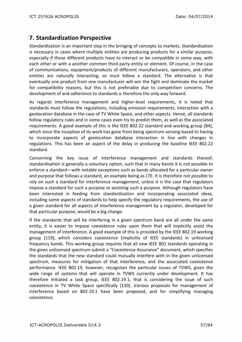
ICT 257626 ACROPOLIS Date: 04/07/2014
ICT-ACROPOLIS Deliverable D14.3 57/84
7. Standardization Perspective
Standardization is an important step in the bringing of concepts to markets. Standardisation
is necessary in cases where multiple entities are producing products for a similar purpose,
especially if those different products have to interact or be compatible in some way, with
each other or with a another common third party entity or element. Of course, in the case
of communications, equipment/products of different manufacturers, operators, and other
entities are naturally interacting, so must follow a standard. The alternative is that
eventually one product from one manufacturer will win the fight and dominate the market
for compatibility reasons, but this is not preferable due to competition concerns. The
development of and adherence to standards is therefore the only way forward.
As regards interference management and higher-level requirements, it is noted that
standards must follow the regulations, including emission requirements, interaction with a
geolocation database in the case of TV White Space, and other aspects. Hence, all standards
follow regulatory rules and in some cases even try to predict them, as well as the associated
requirements. A good example of this is the IEEE 802.22 standard and working group [84],
which since the inception of its work has gone from being spectrum sensing-based to having
to incorporate aspects of geolocation database interaction in line with changes in
regulations. This has been an aspect of the delay in producing the baseline IEEE 802.22
standard.
Concerning the key issue of interference management and standards thereof,
standardisation is generally a voluntary option, such that in many bands it is not possible to
enforce a standard—with notable exceptions such as bands allocated for a particular owner
and purpose that follows a standard, an example being as LTE. It is therefore not possible to
rely on such a standard for interference management, unless it is the case that regulators
impose a standard for such a purpose or assisting such a purpose. Although regulators have
been interested in feeding from standardisation and incorporating associated ideas,
including some aspects of standards to help specify the regulatory requirements, the use of
a given standard for all aspects of interference management by a regulator, developed for
that particular purpose, would be a big change.
If the standards that will be interfering in a given spectrum band are all under the same
entity, it is easier to impose coexistence rules upon them that will implicitly assist the
management of interference. A good example of this is provided by the IEEE 802.19 working
group [119], which considers coexistence (implicitly of IEEE standards) in unlicensed
frequency bands. This working group requires that all new IEEE 802 standards operating in
the given unlicensed spectrum submit a “Coexistence Assurance” document, which specifies
the standards that the new standard could mutually interfere with in the given unlicensed
spectrum, measures for mitigation of that interference, and the associated coexistence
performance. IEEE 802.19, however, recognises the particular issues of TVWS, given the
wide range of systems that will operate in TVWS currently under development. It has
therefore initiated a task group, IEEE 802.19.1, that is considering the issue of such
coexistence in TV White Space specifically [120]. Various proposals for management of
interference based on 802.19.1 have been proposed, and for simplifying managing
coexistence.

ICT 257626 ACROPOLIS Date: 04/07/2014
ICT-ACROPOLIS Deliverable D14.3 58/84
7.1 Limits on the aggregate interference
Following the actions undertaken by the US FCC that opened up significant parts of the TV
spectrum for unlicensed use, other countries in the world have considered to apply similar
measures [121] [122] [123]. The FCC selected a value of the maximum transmit power for
devices operating in the White Spaces in unlicensed fashion. The FCC also defined the so
called erosion margin, which quantifies how much the TV service can degrade and thus the
tolerable amount of interference that CR devices can inject in TV bands. A zero erosion
margin would imply zero white spaces. This margin is particularly important as it allows
determining how far the CR devices (referred to as White Spaces Devices) have to be from
television receivers, taking into account in-band interference and the interference caused by
transmissions on adjacent channels.
As seen from the literature related to this topic, interferences (intentional or unintentional)
represent one of the major challenges from the perspective of designers. The interference is
not only intended as the degradation of a primary service (e.g., televisions service) and thus
the need to protect it but also to the fact that the TV broadcasting service will affect CR
devices. This latter aspect is known as pollution [124]. The aspect of interference is strictly
connected to the concept of how much a radio system can be interfered before
experiencing performance degradation. The higher is the resilience the more a system could
operate in hostile (i.e., interfered in this case) environments. Initial estimations of the White
Spaces and of interference margins have started in the USA but similar ones can be found in
Europe as well. For example, [63] shows calculation of the maximum interfering power and
field strength that a primary service can tolerate in case of the TV broadcasting service,
PMSE systems, radio astronomy services and aeronautical navigation systems.
7.2 TV White Spaces estimation in the USA
The work done in the seminal papers [124] and [125] represented a fundamental step to
understand the amount of White Spaces that could be available for communications before
and after the digital switch-over (DSO) of analog TV. A similar work for Europe is available
from [126], whereas a test bed used to measure the amount of White Spaces in the UK is
available from [129].
The work done in [124] deems to evaluate the amount of White Spaces that are available in
the USA for cognitive radios, with a 6 MHz TV channel width and a 4 W of equivalent
radiated power (ERP). Here it is taken an approach that includes the protection viewpoint
(for protecting the receivers of the primary service from the aggregate interference) and
pollution viewpoint (the primary service affecting the availability and quality of spectrum for
cognitive devices). Results are in terms of the average number of white space channels per
location (this accounts for the area as normalization factor) or per person (this accounts for
the population density as normalization factor). The study, regardless of the viewpoint,
assumes the FCC’s transmitters database and the ITU propagation model (ITU-R P-1536-3).
The results are shown for UHF and VHF frequency bands considering different acceptable
pollution levels with and without adjacent channels interference (i.e., in this case TV
transmitters operating on channels other than the selected one). White space channels for
the pollution viewpoint are more available in the low VHF band. For the protection
viewpoint, with a zero watt transmitter, there are almost 19 white space channels per
person in the low UHF. However, as soon as the transmit power of the secondary users is
increased this number reduces dramatically. When also fading is taken into account, the

ICT 257626 ACROPOLIS Date: 04/07/2014
ICT-ACROPOLIS Deliverable D14.3 59/84
erosion margin introduced in the previous section is found to be around 1dB, as ruled out by
the FCC. Beyond an erosion margin of 0.1 dB, there is a gain of almost 20 available white
space channels per person.
The work done in [125] deems to evaluate the available capacity (intended as the Shannon
information-theoretic capacity) within the White Spaces throughout the US, fulfilling also
the FCC constraints for the protection of the TV service. The computation is carried out
applying propagation models approved by the FCC for this matter. For a TV channel of 6
MHz width, a TV signal with 4 W ERP in each channel and a single link of 1 Km and 10 Km,
the result shows a huge amount of White Spaces. As pointed out by the authors this result is
misleading as a single link is not a meaningful target. As soon as the effect of interference
piles up, the amount of White Spaces changes dramatically. Two important aspects are
highlighted by this work: the importance of the propagation models that are selected and
the regulatory aspects incorporated which greatly affect the final result and the definition of
an exclusion-radius, which is the real footprint of a White Space transmitter for the purpose
of sharing. A very interesting insight is provided by dividing the capacity of White Spaces in a
given area by the population density. This shows that, on a long term, a user receives up to
10 Kbits/sec which goes up to 720 Kbits/sec over a shorter term. The paper concludes with
an insight of economic effects that arise from using White Spaces taking again into
consideration the density of people.
7.3 TV White Spaces in the European Context
The work done in [126] is one of the first attempts to quantify the amount of White Spaces
available in Europe and it is somewhat similar to [124] and [125]. The study investigates the
situation of White Spaces in Europe taking into account the area of interest and density of
the population. The erosion margin is set to 1 dB and the frequency range is 470-790 MHz,
which is what remains of the European digital dividend. In terms of propagation models, it is
used the ITU model and the Longley-Rice irregular terrain model. The study, with and
without adjacent channels interference, is conducted for European countries like Austria
Belgium, Czech republic, Denmark, Germany, The Netherlands, Luxemburg, Slovakia,
Sweden, Switzerland and the United Kingdom. The approach, if compared to the previous
papers already cited, is based on the protection viewpoint. Using TV network data, for the
United Kingdom, this study managed to derive the protection region before and after the
switch-over of analogue TV in terms of the minimum field strength. Thus, the required field
strength in dB is computed as follows
,1.150log20
5.111log20
10
)(
10
log)(
req
Digital
Ana
SNRfE
fE
+−+=
−+=
γ
γ
(74)
Where γ is the erosion margin and SNRreq is the value required to protect the TV service. The
study confirms that the amount of White Spaces available in Europe is less than in the USA,
as also stated in [127]. For the entire evaluated European region the average availability of
white space channels is around 25% by area compared to the USA (or 18% by population).
Based on various academic, industrial and regulatory input the ECC produced its landmark
report ECC159 in January 2011 on the technical and operational requirements for the use of
cognitive radio in TV white space in 470-790 MHz band. The report considers the use of
sensing and geolocation-based approaches to minimise risk of harmful interference to the
incumbents. The following incumbent protection cases are considered:
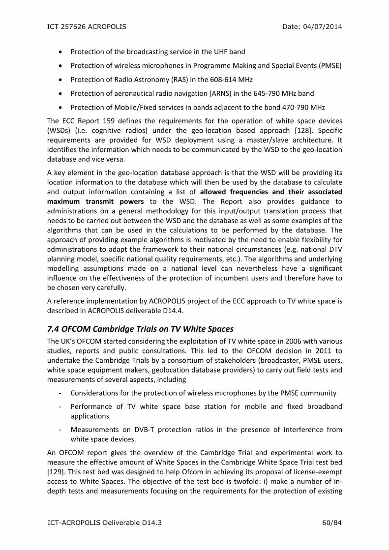
ICT 257626 ACROPOLIS Date: 04/07/2014
ICT-ACROPOLIS Deliverable D14.3 60/84
• Protection of the broadcasting service in the UHF band
• Protection of wireless microphones in Programme Making and Special Events (PMSE)
• Protection of Radio Astronomy (RAS) in the 608-614 MHz
• Protection of aeronautical radio navigation (ARNS) in the 645-790 MHz band
• Protection of Mobile/Fixed services in bands adjacent to the band 470-790 MHz
The ECC Report 159 defines the requirements for the operation of white space devices
(WSDs) (i.e. cognitive radios) under the geo-location based approach [128]. Specific
requirements are provided for WSD deployment using a master/slave architecture. It
identifies the information which needs to be communicated by the WSD to the geo-location
database and vice versa.
A key element in the geo-location database approach is that the WSD will be providing its
location information to the database which will then be used by the database to calculate
and output information containing a list of allowed frequencies and their associated
maximum transmit powers to the WSD. The Report also provides guidance to
administrations on a general methodology for this input/output translation process that
needs to be carried out between the WSD and the database as well as some examples of the
algorithms that can be used in the calculations to be performed by the database. The
approach of providing example algorithms is motivated by the need to enable flexibility for
administrations to adapt the framework to their national circumstances (e.g. national DTV
planning model, specific national quality requirements, etc.). The algorithms and underlying
modelling assumptions made on a national level can nevertheless have a significant
influence on the effectiveness of the protection of incumbent users and therefore have to
be chosen very carefully.
A reference implementation by ACROPOLIS project of the ECC approach to TV white space is
described in ACROPOLIS deliverable D14.4.
7.4 OFCOM Cambridge Trials on TV White Spaces
The UK’s OFCOM started considering the exploitation of TV white space in 2006 with various
studies, reports and public consultations. This led to the OFCOM decision in 2011 to
undertake the Cambridge Trials by a consortium of stakeholders (broadcaster, PMSE users,
white space equipment makers, geolocation database providers) to carry out field tests and
measurements of several aspects, including
- Considerations for the protection of wireless microphones by the PMSE community
- Performance of TV white space base station for mobile and fixed broadband
applications
- Measurements on DVB-T protection ratios in the presence of interference from
white space devices.
An OFCOM report gives the overview of the Cambridge Trial and experimental work to
measure the effective amount of White Spaces in the Cambridge White Space Trial test bed
[129]. This test bed was designed to help Ofcom in achieving its proposal of license-exempt
access to White Spaces. The objective of the test bed is twofold: i) make a number of in-
depth tests and measurements focusing on the requirements for the protection of existing

ICT 257626 ACROPOLIS Date: 04/07/2014
ICT-ACROPOLIS Deliverable D14.3 61/84
services and ii) help industry to understand the benefits arising from White Space spectrum.
The test bed consists of 8 base stations deployed in urban and rural environments with 5
assigned in urban locations. The technology used includes 6Harmonics, Adaptrum, KTS and
Neul. In urban locations, the maximum allowed transmitted power was set in the order of
125 dBm of EIRP for base stations and mobile terminals. For rural areas the tested link
included a directional antenna transmitting over a distance of approximately 6 Km. Tests ran
from August to November 2011 in UHF bands. Plots of experimental data, after processing,
show that the use of spectrum is reasonably stable over a time scale of months and mostly
clear of harmful interference. One interesting finding of this experimental study was the
provision of a broadband Internet service in rural areas through white space technology.
The broadband access achieved nearly 8 Mbits/sec in downlink and 1.5 Mbits/sec in uplink.
This trial also allowed concluding that a path loss of 140 dB constitutes the minimum
requirement for the provision of the broadband service.
7.5 Protection of PMSE Applications
The PMSE (Programme making and special events) use case represents a socially and
economically important professional user community that already shares the TV white
spaces with broadcasters in the UK and elsewhere. It includes large outdoor concerts,
outdoor collection of footage for news gathering and TV programmes, and widespread use
of wireless microphones in theatres and conference halls.
In order to protect PMSE, relevant EIRP restrictions need to be applied on WSDs operating
in the geographic cells around the PMSE events. A cell is typically defined as a 100m x 100m
pixel. The protection approach is to limit the interference at the PMSE receiver such that the
sensitivity of the equipment is not degraded beyond an acceptable margin [130, 131].
To achieve this, the interference from WSD, weighted by the receiver ACS value should be in
the range below the receiver’s noise floor. Figure 7-1 shows the degradation in receiver
sensitivity as function of I/N [130].
Figure 7-1: Degradation in receiver sensitivity as function of l/N [130]

ICT 257626 ACROPOLIS Date: 04/07/2014
ICT-ACROPOLIS Deliverable D14.3 62/84
(a) Reference geometry between a PMSE receiver and the WSD transmitter
(b) Scenario: Outdoor events e.g. Street fair, foot race, etc
(c) Indoor scenario: Concert hall, theatre, etc
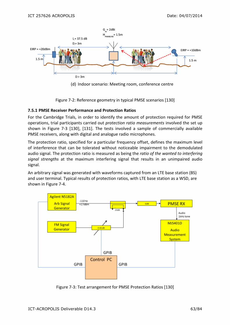
ICT 257626 ACROPOLIS Date: 04/07/2014
ICT-ACROPOLIS Deliverable D14.3 63/84
(d) Indoor scenario: Meeting room, conference centre
Figure 7-2: Reference geometry in typical PMSE scenarios [130]
7.5.1 PMSE Receiver Performance and Protection Ratios
For the Cambridge Trials, in order to identify the amount of protection required for PMSE
operations, trial participants carried out protection ratio measurements involved the set up
shown in Figure 7-3 [130], [131]. The tests involved a sample of commercially available
PMSE receivers, along with digital and analogue radio microphones.
The protection ratio, specified for a particular frequency offset, defines the maximum level
of interference that can be tolerated without noticeable impairment to the demodulated
audio signal. The protection ratio is measured as being the ratio of the wanted to interfering
signal strengths at the maximum interfering signal that results in an unimpaired audio
signal.
An arbitrary signal was generated with waveforms captured from an LTE base station (BS)
and user terminal. Typical results of protection ratios, with LTE base station as a WSD, are
shown in Figure 7-4.
Figure 7-3: Test arrangement for PMSE Protection Ratios [130]

ICT 257626 ACROPOLIS Date: 04/07/2014
ICT-ACROPOLIS Deliverable D14.3 64/84
(a) LTE base station interference at 100% traffic
(b) LTE base station interference at 50% traffic
Figure 7-4: Protection ratios for PMSE from LTE base station as a WSD [130]
The test indicated that protection ratio values for both the high and low power wanted
signals are different; the worse adjacent channel protection ratio for the -30dBm wanted
signal is as a result of the receiver being overloaded (both wanted and interfering signal
powers are large in this case).
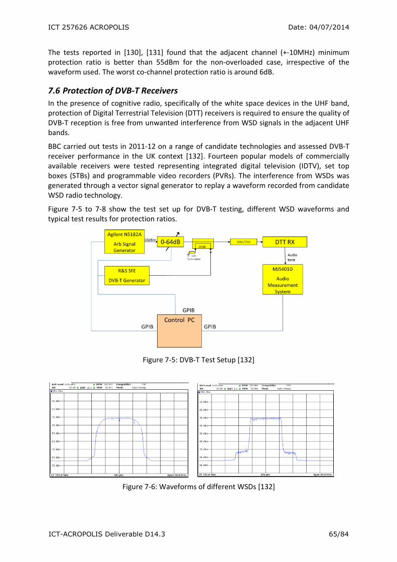
ICT 257626 ACROPOLIS Date: 04/07/2014
ICT-ACROPOLIS Deliverable D14.3 65/84
The tests reported in [130], [131] found that the adjacent channel (+-10MHz) minimum
protection ratio is better than 55dBm for the non-overloaded case, irrespective of the
waveform used. The worst co-channel protection ratio is around 6dB.
7.6 Protection of DVB-T Receivers
In the presence of cognitive radio, specifically of the white space devices in the UHF band,
protection of Digital Terrestrial Television (DTT) receivers is required to ensure the quality of
DVB-T reception is free from unwanted interference from WSD signals in the adjacent UHF
bands.
BBC carried out tests in 2011-12 on a range of candidate technologies and assessed DVB-T
receiver performance in the UK context [132]. Fourteen popular models of commercially
available receivers were tested representing integrated digital television (IDTV), set top
boxes (STBs) and programmable video recorders (PVRs). The interference from WSDs was
generated through a vector signal generator to replay a waveform recorded from candidate
WSD radio technology.
Figure 7-5 to 7-8 show the test set up for DVB-T testing, different WSD waveforms and
typical test results for protection ratios.
Figure 7-5: DVB-T Test Setup [132]
Figure 7-6: Waveforms of different WSDs [132]
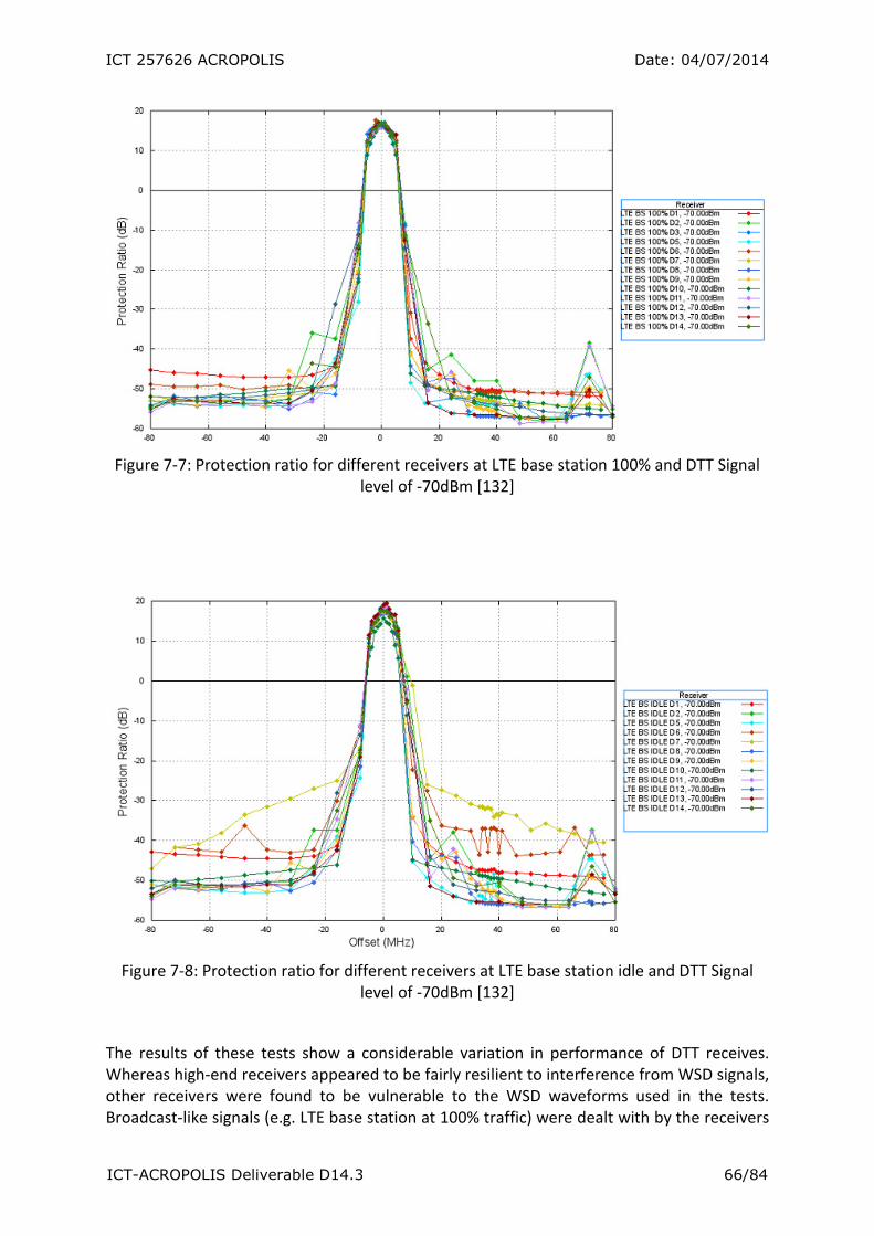
ICT 257626 ACROPOLIS Date: 04/07/2014
ICT-ACROPOLIS Deliverable D14.3 66/84
Figure 7-7: Protection ratio for different receivers at LTE base station 100% and DTT Signal
level of -70dBm [132]
Figure 7-8: Protection ratio for different receivers at LTE base station idle and DTT Signal
level of -70dBm [132]
The results of these tests show a considerable variation in performance of DTT receives.
Whereas high-end receivers appeared to be fairly resilient to interference from WSD signals,
other receivers were found to be vulnerable to the WSD waveforms used in the tests.
Broadcast-like signals (e.g. LTE base station at 100% traffic) were dealt with by the receivers

ICT 257626 ACROPOLIS Date: 04/07/2014
ICT-ACROPOLIS Deliverable D14.3 67/84
without interference. However, burst-like signals (e.g. low traffic CPE signals) result in up to
a 30dB degradation in protection ratios.
As a consequence, the authors in [132] recommend the use of a highly conservative
protection ratio values in the UK in order to protect the majority of existing consumer grade
DVB-T receivers (largely in the form of low cost set-top boxes used to adapt old analogue TV
receivers to DTT reception). The authors concluded that the geolocation database approach
to TVWS was feasible provided that the database could take into consideration the various
WS technologies and the predicted field strength at the DTT receiver location.
7.7 Spectrum and Environment Measurements Supporting Interference
Prediction and Assessment
Spectrum and environment measurements for general characterisation purposes are key
ways of assessing both the availability of spectrum for opportunistic use and other forms of
sharing, and the potential interference that could result. Moreover, in-the-field
measurements, aligned with estimation approaches in some scenarios represent means of
monitoring, locating and mapping potential interference effects.
One area in which some extensive related work has been done given its interest in the
community and given a number of positive initiatives in regulatory circles is TV white spaces.
The prior sections have concentrated heavily on aspects of TV white spaces. Here we
concentrate more generally on other bands.
Within ICT-ACROPOLIS, extensive measurements have been done within in London in July
2011 (see, e.g., [133], [134]). These measurements and the ensuing analysis concentrate
heavily on correlation aspects of the traffic, and particularly temporal and spatial
correlation, both of which have profound implications for the characteristics of the
availability of spectrum for sharing, and associated design implications for the systems that
must implement sharing. The measurements assessing temporal correlation were taken at a
fixed location for a long duration, whereas the measurements assessing spatial correlation
were done through maintaining one measurement system at a fixed location, and moving
other measurements systems with respect to that, ensuring that the times of the
measurements are accurately logged so that the measurements from exact the same time
can be compared thereby ruling out temporal variation effects in assessing the spatial
comparison. Such a concept could be implemented through drive testing, as covered in
Deliverable 9.3 [135], were such drive-testing supported by the time-stamps of a GPS
system, for example. Moreover, the understanding of correlation aspects through such
measurements can assist in the calculations done by radio environment mapping, also
covered in Deliverable 9.3, noting that there is a direct link between correlation and
variance, which of course exists by definition if the covariance measure is used.
In [133], spatial correlation aspects have been assessed at a number of different locations in
London as part of the July 2011 campaign. On the one hand this work applies the semi-
variogram measure to assess spatial correlation, letting the parameter of the semivariogram
be the distance between measurement locations considered, instead of a time or frequency
separation. In this case the natural estimator for the spatial semivariogram becomes the
empirical variogram of Matheron. The main challenge in applying this semivariogram
definition to the data set is that the number of individual measurement locations within a
measurement area is not very large, resulting in a high estimation variance at an individual
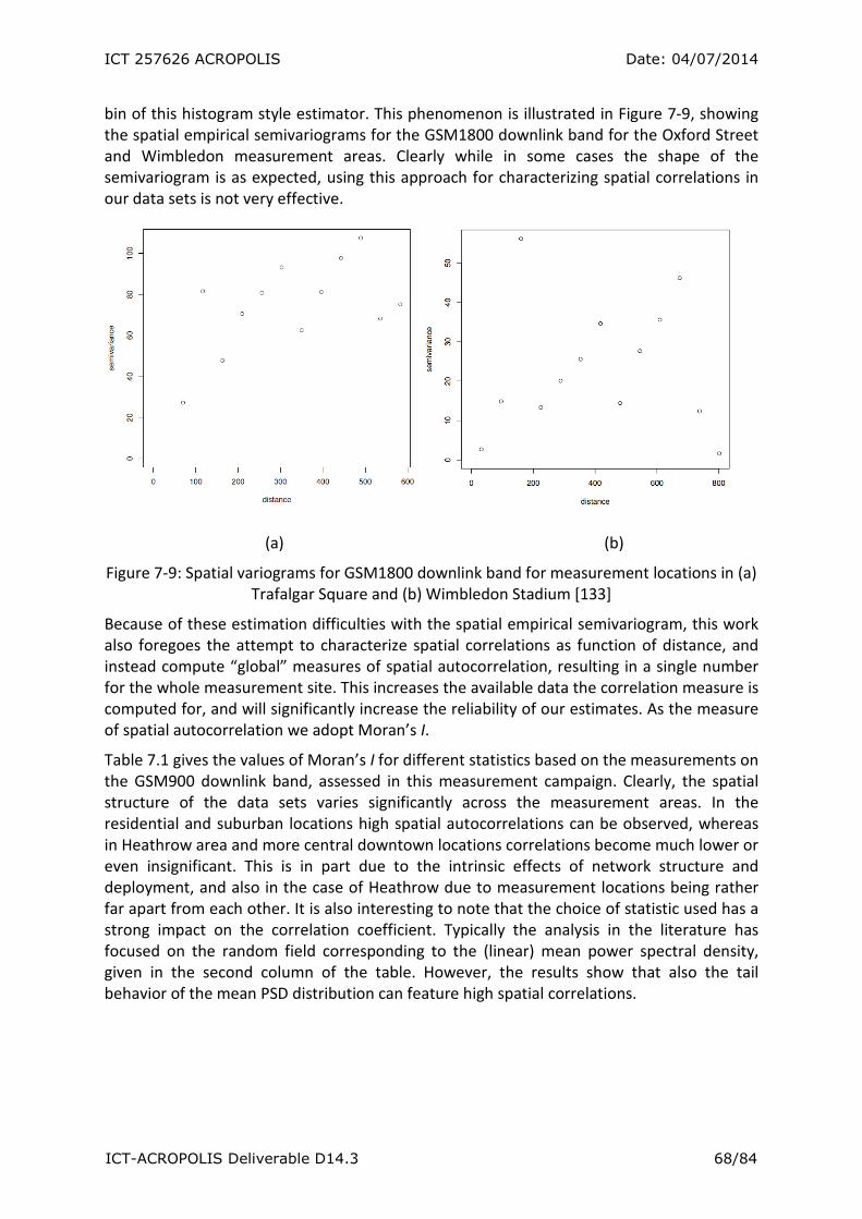
ICT 257626 ACROPOLIS Date: 04/07/2014
ICT-ACROPOLIS Deliverable D14.3 68/84
bin of this histogram style estimator. This phenomenon is illustrated in Figure 7-9, showing
the spatial empirical semivariograms for the GSM1800 downlink band for the Oxford Street
and Wimbledon measurement areas. Clearly while in some cases the shape of the
semivariogram is as expected, using this approach for characterizing spatial correlations in
our data sets is not very effective.
(a) (b)
Figure 7-9: Spatial variograms for GSM1800 downlink band for measurement locations in (a)
Trafalgar Square and (b) Wimbledon Stadium [133]
Because of these estimation difficulties with the spatial empirical semivariogram, this work
also foregoes the attempt to characterize spatial correlations as function of distance, and
instead compute “global” measures of spatial autocorrelation, resulting in a single number
for the whole measurement site. This increases the available data the correlation measure is
computed for, and will significantly increase the reliability of our estimates. As the measure
of spatial autocorrelation we adopt Moran’s I.
Table 7.1 gives the values of Moran’s I for different statistics based on the measurements on
the GSM900 downlink band, assessed in this measurement campaign. Clearly, the spatial
structure of the data sets varies significantly across the measurement areas. In the
residential and suburban locations high spatial autocorrelations can be observed, whereas
in Heathrow area and more central downtown locations correlations become much lower or
even insignificant. This is in part due to the intrinsic effects of network structure and
deployment, and also in the case of Heathrow due to measurement locations being rather
far apart from each other. It is also interesting to note that the choice of statistic used has a
strong impact on the correlation coefficient. Typically the analysis in the literature has
focused on the random field corresponding to the (linear) mean power spectral density,
given in the second column of the table. However, the results show that also the tail
behavior of the mean PSD distribution can feature high spatial correlations.
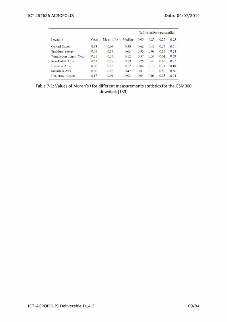
ICT 257626 ACROPOLIS Date: 04/07/2014
ICT-ACROPOLIS Deliverable D14.3 69/84
Table 7-1: Values of Moran’s I for different measurements statistics for the GSM900
downlink [133]

ICT 257626 ACROPOLIS Date: 04/07/2014
ICT-ACROPOLIS Deliverable D14.3 70/84
8. Conclusions
This report has focused on the issue of interference generated by cognitive radio networks
to primary user communications, as well as other spectrum sharing cases, particularly
concentrating on the issue of aggregate interference. The proliferation of innovative
wireless technologies and corresponding services lead to the serious problem of spectrum
shortage. The paradigm of cognitive radio, as well as other spectrum sharing regimes, may
therefore represent a possible solution that opens the way to unconventional forms of use
that deviate from the typical command and control or exclusive use ideology.
Such agile spectrum access where cognitive radios might access different frequency bands,
anytime and anywhere, requires particular attention to the problem of aggregate
interference. Most of the work behind cognitive radio is founded on the assumptions that
cognitive radio devices can detect the presence of the primary user’s transmissions and they
do not cause significant degradation of the licensee’s performance. Even if only one of these
assumptions doesn’t carry, the concept of cognitive radio is of greatly reduced importance
and viability. Accordingly, sophisticated analytical and simulation tools are needed to
predict the impact of aggregate interference on the performance of the primary user.
The relevant scenarios for addressing the important problem of interference in this
document have been selected among the existing taxonomy of spectrum sharing principles.
Therefore, the selected scenarios were: TV White Spaces, Femtocells, UWB and spectrum
sharing among equal unlicensed users. This deliverable has reviewed existing approaches
that have been adopted for modelling of the aggregate interference throughout time. The
starting point is the observation that the typical Gaussian approximation of the aggregate
interfering process that pours out from the application of the central limit theorem is
appealing but at the same time wrong. Beside analytical tools, this deliverable has spent
some time reviewing existing simulation tools for estimating the impact of wireless
interference. Among the variety of existing tools, this deliverable paid particular attention
on the SEAMCAT simulator developed within CEPT.
The most advanced analytical tools used for modelling aggregate interference borrow
concepts from stochastic geometry. The most widely used assumption is that nodes are
scattered over space according to a homogeneous Poisson point process. This assumption
allows for analytical tractability although not completely realistic. Results originated from
the application of stochastic geometry as well as from standard probability theory lead to
the conclusion that the distribution of the aggregate interference power belongs to the
family of heavy tail distributions known as stable distributions. It was also shown that
realistic propagation effects (e.g., fading) are reflected in the computation of the
parameters of the stable distribution. Recent papers have the merit of empowering the
analysis also with the capability of accounting for specific sensing schemes, cooperation
among the secondary users and different positions of the primary receivers.
This report has shown that the design of a wireless cognitive system cannot be made
without accounting for the effect of the aggregate interference they could generate. This
aspect should gain increasing relevance and never be neglected in any future design. As the
Poisson displacement of the nodes is not completely realistic, more studies on aggregate
interference modelling, simulations as well as measurements are needed.
ICT 257626 ACROPOLIS Date: 04/07/2014
ICT-ACROPOLIS Deliverable D14.3 71/84
Finally, in recent years, practical work in the UK under “The OFCOM Cambridge Trials on TV
white spaces”) has focussed on determining the safe conditions for the deployment of
cognitive radio in the UHF band. Based on the measurements carried out in the trials,
participants have established the protection ratios for the incumbents (DTT and PMSE users)
to determine the maximum WSD power levels and channel separation from the incumbents.
These protection ratios will form the basis of regulatory limits in future while considering
the allowable use of different white space technologies by secondary users while minimising
the risk of harmful interference to primary users.

ICT 257626 ACROPOLIS Date: 04/07/2014
ICT-ACROPOLIS Deliverable D14.3 72/84
Appendix. A short tutorial on stochastic geometry
This section is devoted to summarize some general concepts of stochastic geometry that are
useful to understand how models of the aggregate interference can be developed.
Definition A1: A set A has the following properties
1. It is said to be open if for each x in A it exists a positive real number ε>0
such Axb ⊂),( ε , where b(x,ε) denotes the ball centred at x and with radius ε.
2. it is closed if its complement Ac is open.
3. It is bounded if ),( rabA⊂ for r>0 and a location point a.
4. the interior of the set is the union of all open sets contained in A.
5. the closure of A is the intersection of all closed sets containing A.
6. A set ⊂A d is said to be compact if it is closed and bounded.
Definition A2: In measure theory, the concept of σ-algebra is a system χ of subsets of a set
Ax satisfying the following properties
1. Ax ϵ χ
2. If Ax ϵ χ then Acx ϵ χ
3. If ∈,..., 21 AA χ then U∞
=
∈1x
xA χ
4. ∈0 χ
5. If ∈,..., 21 AA χ then ∈21 \ AA χ
6. If ∈,..., 21 AA χ then ∈∞
=I
1x
xA χ
7. If ∈nAAA ,...,, 21 χ then Un
x
xA1=
∈ χ and ∈=In
x
xA1
χ
Remark A1: The family of Borel sets BBBB d
on d represents the smallest possible σ-algebra.
Remark A2: In order to develop the concepts related to measure theory, the following facts
are going to be used:
1. A set Ax and its σ-algebra constitute a measurable space,
2. A function f: Ax-> is said to be χ-measurable if for all Borel sets B ϵ BBBB 1
the inverse
image f-1
(B)=x ϵ Ax : f(x) ϵ B belongs to the σ-algebra χ associated with Ax.
Definition A3: A particular example of measurable function is the indicator function of a
measurable set A
1111A
∈
=otherwise
Axfor x
0
1
Definition A4: The measure on [χ,Ax] is a function :µ χ ],0[ ∞>− satisfying the following
properties
- μ(0)=0,
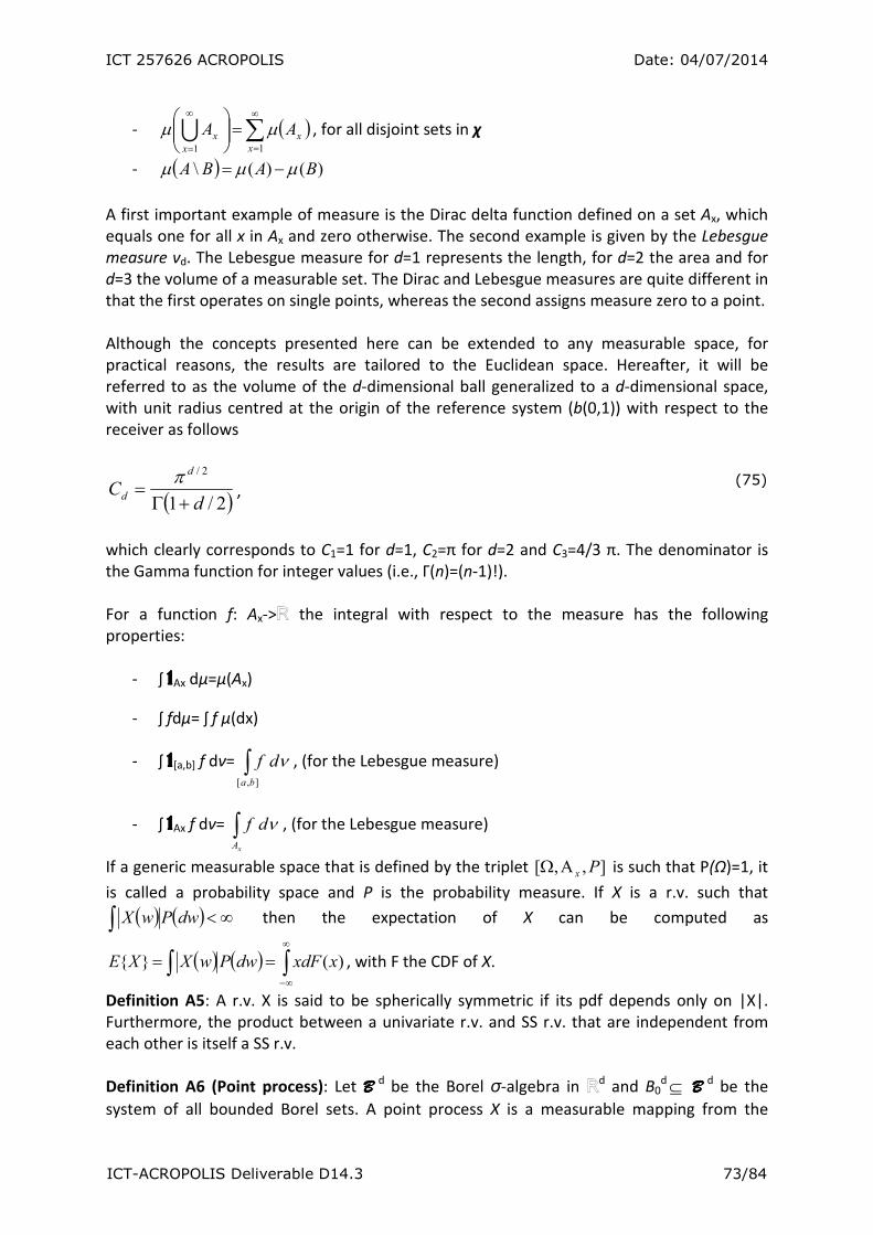
ICT 257626 ACROPOLIS Date: 04/07/2014
ICT-ACROPOLIS Deliverable D14.3 73/84
- ( )∑∞
=
∞
=
=
11 x
x
x
x AA µµ U , for all disjoint sets in χ
- ( ) )()(\ BABA µµµ −=
A first important example of measure is the Dirac delta function defined on a set Ax, which
equals one for all x in Ax and zero otherwise. The second example is given by the Lebesgue
measure νd. The Lebesgue measure for d=1 represents the length, for d=2 the area and for
d=3 the volume of a measurable set. The Dirac and Lebesgue measures are quite different in
that the first operates on single points, whereas the second assigns measure zero to a point.
Although the concepts presented here can be extended to any measurable space, for
practical reasons, the results are tailored to the Euclidean space. Hereafter, it will be
referred to as the volume of the d-dimensional ball generalized to a d-dimensional space,
with unit radius centred at the origin of the reference system (b(0,1)) with respect to the
receiver as follows
( )2/1
2/
dC
d
d +Γ=
π,
(75)
which clearly corresponds to C1=1 for d=1, C2=π for d=2 and C3=4/3 π. The denominator is
the Gamma function for integer values (i.e., Γ(n)=(n-1)!).
For a function f: Ax-> the integral with respect to the measure has the following
properties:
- ʃ 1111Ax dμ=μ(Ax)
- ʃ fdμ= ʃ f μ(dx)
- ʃ 1111[a,b] f dν= ∫],[
ba
df ν , (for the Lebesgue measure)
- ʃ 1111Ax f dν= ∫xA
df ν , (for the Lebesgue measure)
If a generic measurable space that is defined by the triplet ],,[ PxΑΩ is such that P(Ω)=1, it
is called a probability space and P is the probability measure. If X is a r.v. such that
( ) ( )∫ ∞<dwPwX then the expectation of X can be computed as
( ) ( )∫ ∫∞
∞−
== )( xxdFdwPwXXE , with F the CDF of X.
Definition A5: A r.v. X is said to be spherically symmetric if its pdf depends only on |X|.
Furthermore, the product between a univariate r.v. and SS r.v. that are independent from
each other is itself a SS r.v.
Definition A6 (Point process): Let BBBB d
be the Borel σ-algebra in d and B0
d ⊆ BBBB d
be the
system of all bounded Borel sets. A point process X is a measurable mapping from the

ICT 257626 ACROPOLIS Date: 04/07/2014
ICT-ACROPOLIS Deliverable D14.3 74/84
abstract probability space ],,[ PxΑΩ to ⊆= xN lf
d ( ) dB BBxn 0: ∈∞∀< , where
BxxB ∩= and n(xB) denotes the cardinality of the set. Furthermore, when Nlf is equipped
with a σ-algebra it implies that n(xB)=N, ∈∀N .
Proposition A1 (Random point): Let us consider a point ξ uniformly distributed in a
compact set ⊂Wd. This point is a random point if for all Borel sets WB ⊂ it holds that
)(
)(
W
BP
d
d
νν
ξ = . (76)
As a consequence, a random-point pattern of n points ( nξξ ...,1 ) uniformly distributed over
space forms a BPP.
For the sake of completeness, the useful summary on the properties of a spatial point
process on the Euclidean space d given in [104] allows a few dichotomies:
- A PP is said to be simple if the multiplicity of a point over space is one; otherwise it is
not
- A PP is said to be stationary if the resulting spatial process results invariant by
translation.
- A PP is said to be isotropic if the resulting spatial process is invariant to rotation.
- A PP is said to be marked if it assigns labels to the points of the process, which are
typically independent of the PP.
- A PP can be Poisson or not. If it is Poisson, it can be homogeneous or non-
homogeneous, as it was discussed in Section 4.4.
It is important to remark that a homogeneous PPP is both stationary and simple.

ICT 257626 ACROPOLIS Date: 04/07/2014
ICT-ACROPOLIS Deliverable D14.3 75/84
9. References
[1] J. Mitola, “Cognitive radio: An Integrated Agent Architecture for Software Defined
Radio,” Ph.D. dissertation, KTH Royal Inst. of Technol., Stockholm, Sweden, 2000.
[2] D13.2, “Context and Interference Aware Coding and Decoding”. ACRPOPOLIS
deliverable, Nov. 2012.
[3] FCC, “Policy Task Force Report (et docket-135)”, 2002.
[4] M. A. McHenry, “NSF Spectrum Occupancy Measurements Project Summary,” Shared
Spectrum Company, 2005.
[5] FCC, “Notice of proposed rulemaking, in the matter of facilitating opportunities for flexible,
efficient and reliable spectrum use employing cognitive radio technologies (et docket no. 03-
108) and authorization and use of software defined radios (et docket no. 00-47), FCC 03-
322,” Dec. 2003.
[6] S. Haykin, “Cognitive radio: Brain-empowered wireless communications,” IEEE J. Sel. Areas
Commun., vol. 23, no. 2, pp. 201–220, Feb. 2005.
[7] I. F. Akyildiz, W. Lee, M. C. Vuran, and S. Mohanty, “Next Generation/Dynamic Spectrum
Access/Cognitive Radio Wireless Networks: A Survey,” Computer Networks, vol. 50, no. 13,
pp. 2127–2159, Sep. 2006.
[8] Q. Zhao and B. M. Sadler, “A Survey of Dynamic Spectrum Access,” IEEE Signal Process.
Mag., vol. 24, no. 3, pp. 79–89, May 2007.
[9] A. Goldsmith, S. A. Jafar, I. Maric, and S. Srinivasa, “Breaking Spectrum Gridlock with
Cognitive Radios: An Information Theoretic Perspective,”Proc. IEEE, vol. 97, no. 5, pp. 894–
914, May 2009.
[10] A. Ghasemi, and E. S. Sousa, “Spectrum Sensing in Cognitive Radio Networks: Requirements,
Challenges and Design Trade-Offs,” IEEE Commun. Mag., vol. 46, no. 4, pp. 32–39, Apr. 2008.
[11] Cabric, S. M. Mishra, and R. W. Brodersen, “Implementation Issues in Spectrum Sensing for
Cognitive Radios,” in Proc. Asilomar Conf. on Signals, Systems, and Computers, Pacific, Grove,
Nov. 2004, pp. 772– 776.
[12] A. Sonnenschein and P. M. Fishman, “Radiometric Detection of Spread- Spectrum Signals in
Noise,” IEEE Trans. Aerosp. Electron. Syst., vol. 28, no. 3, pp. 654–660, Jul. 1992.
[13] R. Tandra and A. Sahai, “SNR Walls for Signal Detection,” IEEE J. Sel. Topics Signal Process.,
vol. 2, no. 1, pp. 4–17, Feb. 2008.
[14] R. Tandra, S. M. Mishra, and A. Sahai, “What is a Spectrum Hole and What Does It Take to
Recognize One Extended Version,” Proc. IEEE, vol. 97, no. 5, pp. 824–848, May 2009.
[15] M. Z. Win, “A Mathematical Model for Network Interference,” IEEE Communication Theory
Workshop, Sedona, AZ, May 2007.
[16] M. Z. Win, P. C. Pinto, and L. A. Shepp, “A Mathematical Theory of Network Interference and
its Applications,” Proc. IEEE, vol. 97, no. 2, pp. 205–230, Feb. 2009, special issue on Ultra-
Wide Bandwidth (UWB) Technology & Emerging Applications.
[17] M. Z. Win and R. A. Scholtz, “Impulse radio: How it works,” IEEE Commun. Lett., vol. 2, no. 2,
pp. 36–38, Feb. 1998.

ICT 257626 ACROPOLIS Date: 04/07/2014
ICT-ACROPOLIS Deliverable D14.3 76/84
[18] ——, “Ultra-Wide Bandwidth Time-Hopping Spread-Spectrum Impulse Radio for Wireless
Multiple-Access Communications,” IEEE Trans. Com- mun., vol. 48, no. 4, 8p. 679–691, Apr.
2000.
[19] M. Z. Win, “A Unified Spectral Analysis of Generalized Time-Hopping Spread-Spectrum
Signals in the Presence of Timing Jitter,” IEEE J. Sel. Areas Commun., vol. 20, no. 9, pp. 1664–
1676, Dec. 2002.
[20] R. A. Scholtz, “Private Conversation,” University of Southern California, Sep. 1997, Los
Angeles, CA.
[21] J. H. Winters, “Private conversation,” AT&T Labs-Research, Mar. 2001, Middletown, NJ.
[22] L. A. Shepp, “Private conversation,” AT&T Labs-Research, Mar. 2001, Middletown, NJ.
[23] P. C. Pinto and M. Z. Win, “Communication in a Poisson Field of Interferers – Part I:
Interference Distribution and Error Probability,” IEEE Trans. Wireless Commun., vol. 9, no. 7,
pp. 2176–2186, Jul. 2010.
[24] ——, “Communication in a Poisson Field of Interferers – Part II: Channel Capacity and
Interference Spectrum,” IEEE Trans. Wireless Commun., vol. 9, no. 7, pp. 2187–2195, Jul.
2010.
[25] A. Rabbachin, T. Q. Quek, P. C. Pinto, I. Oppermann, and M. Z. Win, “Non-coherent UWB
Communication in the Presence of Multiple Narrowband Interferers,” IEEE Trans. Wireless
Commun., vol. 9, 2010, to appear.
[26] P. C. Pinto, A. Giorgetti, M. Z. Win, and M. Chiani, “A Stochastic Geometry Approach to
Coexistence in Heterogeneous Wireless Networks,” IEEE J. Sel. Areas Commun., vol. 27, no. 7,
pp. 1268–1282, Sep. 2009, special issue on Stochastic Geometry and Random Graphs for
Wireless Networks.
[27] P. C. Pinto and M. Z. Win, “Spectral Characterization of Wireless Networks,” IEEE Wireless
Commun. Mag., vol. 14, no. 6, pp. 27–31, Dec. 2007, special Issue on Wireless Sensor
Networking.
[28] J. F. Kingman, Poisson Processes. Oxford University Press, 1993.
[29] S. Chandrasekhar, “Stochastic Problems in Physics and Astronomy,” Rev. Modern Phys., vol.
15, no. 1, pp. 1–89, Jan. 1943.
[30] S. E. Heath, “Applications of the Poisson Model to Wireless Telephony and to Cosmology,”
Ph.D. dissertation, Department of Statistics, Rutgers University, Piscataway, NJ, Mar. 2004,
thesis advisor: Professor Lawrence A. Shepp.
[31] M. Y. Vardi, L. Shepp, and L. Kaufman, “A statistical Model for Positron Emission
Tomography,” J. of the American Statistical Association, vol. 80, no. 389, pp. 8–20, Mar.
1985.
[32] M. Beil, F. Fleischer, S. Paschke, and V. Schmidt, “Statistical Analysis of 3D Centromeric
Heterochromatin Structure in Interphase Nuclei,” Journal of Microscopy, vol. 217, pp. 60–68,
2005.
[33] D. L. Snyder, “Filtering and Detection for Doubly Stochastic Poisson Processes,” IEEE Trans.
Inf. Theory, vol. 18, no. 1, pp. 91–102, Jan. 1972.
[34] J. R. Pierce, “Optical Channels: Practical Limits with Photon-Counting,” IEEE Trans. Inf.
Theory, vol. 26, no. 12, pp. 1819–1821, Dec. 1978.
[35] J. R. Pierce, E. C. Posner, and E. R. Rodemich, “The Capacity of the Photon Counting Channel,”
IEEE Trans. Inf. Theory, vol. 27, no. 1, pp. 61–77, Jan. 1981.
ICT 257626 ACROPOLIS Date: 04/07/2014
ICT-ACROPOLIS Deliverable D14.3 77/84
[36] J. L. Massey, “Capacity Cut-off Rate, and Coding for Direct Detection Optical Channel,” IEEE
Trans. Commun., vol. 29, no. 11, pp. 1615–1621, Nov. 1981.
[37] E. S. Sousa, “Performance of a Spread Spectrum Packet Radio Network Link in a Poisson Field
of Interferers,” IEEE Trans. Inf. Theory, vol. 38, no. 6, pp. 1743–1754, Dec. 1992.
[38] J. Ilow, D. Hatzinakos, and A. N. Venetsanopoulos, “Performance of FH SS Radio Networks
with Interference Modelled as a Mixture of Gaussian and Alpha-Stable Noise,” IEEE Trans.
Commun., vol. 46, no. 4, pp. 509– 520, Apr. 1998.
[39] C. C. Chan and S. V. Hanly, “Calculating the Outage Probability in a CDMA Network with
Spatial Poisson Traffic,” IEEE Trans. Veh. Technol., vol. 50, no. 1, pp. 183–204, Jan. 2001.
[40] F. Baccelli, B. Błaszczyszyn, and F. Tournois, “Spatial Averages of Coverage Characteristics in
Large CDMA Networks,” Wireless Networks, vol. 8, no. 6, pp. 569–586, Nov. 2002.
[41] X. Yang and A. P. Petropulu, “Co-channel Interference Modelling and Analysis in a Poisson
Field of Interferers in Wireless Communications,” IEEE Trans. Signal Process., vol. 51, no. 1,
pp. 64–76, 2003.
[42] J. Orriss and S. K. Barton, “Probability Distributions for the Number of Radio Transceivers
which Can Communicate with One Another,” IEEE Trans. Commun., vol. 51, no. 4, pp. 676–
681, Apr. 2003.
[43] S. P. Weber, X. Yang, J. G. Andrews, and G. de Veciana, “Transmission Capacity of Wireless
Ad-hoc Networks with Outage Constraints,” IEEE Trans. Inf. Theory, vol. 51, no. 12, pp. 4091–
4102, Dec. 2005.
[44] O. Dousse, F. Baccelli, and P. Thiran, “Impact of Interferences on Connectivity in Ad-hoc
Networks,” IEEE/ACM Trans. Netw., vol. 13, no. 2, pp. 425–436, Apr. 2005.
[45] O. Dousse, M. Franceschetti, and P. Thiran, “On the Throughput Scaling of Wireless Relay
Networks,” IEEE Trans. Inf. Theory, vol. 52, no. 6, pp. 2756–2761, Jun. 2006.
[46] L. Song and D. Hatzinakos, “Cooperative Transmission in Poisson Distributed Wireless Sensor
Networks: Protocol and Outage Probability,” IEEE Trans. Wireless Commun., vol. 5, no. 10,
pp. 2834–2843, Oct. 2006.
[47] A. Ghasemi and E. S. Sousa, “Interference Aggregation in Spectrum-Sensing Cognitive
Wireless Networks,” IEEE J. Sel. Topics Signal Process., vol. 2, no. 1, pp. 41–56, Feb. 2008.
[48] R. Menon, R. M. Buehrer, and J. H. Reed, “On the Impact of Dynamic Spectrum Sharing
Techniques on Legacy Radio Systems,” IEEE Trans. Wireless Commun., vol. 7, no. 11, pp.
4198–4207, Nov. 2008.
[49] W. Ren, Q. Zhao, and A. Swami, “Power Control in Spectrum Overlay Networks: How to Cross
a Multi-Lane Highway,” IEEE J. Sel. Areas Commun., vol. 27, no. 7, pp. 1283–1296, Sep. 2009.
[50] E. Salbaroli and A. Zanella, “Interference Analysis in a Poisson Field of Nodes of Finite Area,”
IEEE Trans. Veh. Technol., vol. 58, no. 4, pp. 1776–1783, May 2009.
[51] H. Inaltekin, M. Chiang, H. V. Poor, and S. B. Wicker, “The Behaviour of Unbounded Path-Loss
Models and the Effect of Singularity on Computed Network Characteristics,” IEEE J. Sel. Areas
Commun., vol. 27, no. 7, pp. 1078–1092, Sep. 2009.
[52] F. Baccelli, B. Błaszczyszyn, and P. Mu hlethaler, “Stochastic Analysis of Spatial and
Opportunistic Aloha,” IEEE J. Sel. Areas Commun., vol. 27, no. 7, pp. 1105–1119, Sep. 2009.
[53] V. Chandrasekhar and J. G. Andrews, “Uplink Capacity and Interference Avoidance for Two-
Tier Femtocell Networks,” IEEE Trans. Wireless Commun., vol. 8, no. 7, pp. 3498–3509, Jul.
2009.

ICT 257626 ACROPOLIS Date: 04/07/2014
ICT-ACROPOLIS Deliverable D14.3 78/84
[54] A. Rabbachin, T. Q. S. Quek, Shin Hyundong, M. Z. Win, “Cognitive Network
Interference”, IEEE J. Sel. Areas Commun., vol. 29, no. 2, pp. 480–493, Feb. 2011.
[55] A. Rabbachin, T. Q. S. Quek, M. Z. Win, “Statistical Modelling of Cognitive Network
Interference”, IEEE GLOBECOM - Wireless Commun. Symp., 2010.
[56] A. Rabbachin, G. Baldini, T. Q. S. Quek., “Aggregate Interference in White Spaces”, Int. Symp.
on Wireless Commun. Systems, 2010.
[57] R. K. Ganti and M. Haenggi, “Interference and Outage in Clustered Wireless Ad-hoc
Networks,” IEEE Trans. Inf. Theory, vol. 55, no. 9, pp. 4067–4086, Sep. 2009.
[58] K. Gulati, B. L. Evans, J. G. Andrews and K. R. Tinsley, ``Statistics of Co-Channel Interference in
a Field of Poisson and Poisson-Poisson Clustered Interferers'', IEEE Trans. on Signal Proces.,
vol. 58, no. 12, Dec. 2010, pp. 6207-6222.
[59] J. Peha, “Spectrum Sharing Through Spectrum Policy Reform and Cognitive Radio”. Proc. of
the IEEE , vol. 97, no. 4, April 1997.
[60] M. M. Buddhikot, “Understanding Dynamic Spectrum Access: Models, Taxonomy and
Challenges”. Proc. of IEEE Dyspan 2007, 17-21 April 2007.
[61] S. Forge, R. Horvitz and C. Blackman, "Perspectives on the Values of Shared Spectrum
Access".Final Report for the European Commission, Feb. 2012.
[62] P. Kolodzy, “Spectrum Policy Task Force Report”, ET Docket No. 02-135, Nov. 2002.
[63] ECC Report 159 “Technical and operational requirements for the operation of cognitive radio
systems in the ‘white spaces’ of the frequency band 470-790 MHz”.
[64] G. Mansfield, “Femtocells in the US Market-Business Drivers and Consumer Propositions”.
Femtocells EUROPE, ATT, London UK, June 2008.
[65] [61] D. L. Perez, A. Valcarce, G. de la Roche and J. Zhang, “OFDMA Femtocells: A Roadmap on
Interference Avoidance”. IEEE Commun. Mag., Sept. 2009.
[66] K. Zheng, Y. Wang, W. Wang, M. Dohler and J. Wang, “Energy-Efficient Wireless In-Home:
The Need for Interference-Controlled Femtocells”. IEEE Wireless Commun., Dec. 2011.
[67] F. Pantisano, K. Ghaboosi, M. Bennis and R. Verdone, “A self-Organizing Solution for
Interference Avoidance in TDD Underlay Femtocells”. Proc. of the Forty Fourth Asilomar
Conference on Sig. Sys. and Commun., 2010.
[68] L. yang and G. B. Giannakis, “Ultra-Wideband Communications: an Idea Whose Time Has
Come”. IEEE Signal Proc. Mag., vol. 21, no. 6, pp. 26-54, Nov. 2004.
[69] “IEEE std 802.15.4 (2011): Wireless Medium Access Control (MAC) and Physical Layer (PHY)
Specifications for Low Rate Wireless Personal Area Networks (LR-WPANs),” The Institute of
Electrical and Electronics Engineers, Inc., Standard, Roll-up of all IEEE Std 802.15.4 and its
amendments before end of 2011, Sept. 2011.
[70] ECMA-368: High Rate Ultra Wideband PHY and MAC Standard, December 2007.
[71] R. Macchi, "Rev. of UWB and FS Coexistence Report (Annex 5-1)", M1720R0 SE24, CEPT SE24
Meeting 17, Mainz (Germany), Sept. 2002.
[72] R. Giuliano and F. Mazzenga, “On the Coexistence of Power-Controlled Ultrawide-Band
Systems With UMTS, GPS, DCS1800, and Fixed Wireless Systems”. IEEE Trans. on Vehicular
Technology, vol. 54, no. 1, Jan. 2005.
ICT 257626 ACROPOLIS Date: 04/07/2014
ICT-ACROPOLIS Deliverable D14.3 79/84
[73] A. Durantini, R. Giuliano, F. Mazzenga, J. Hernandez and M. B. Villarroya, “Detect and Avoid
Procedure for UWB Interference Mitigation on Narrowband Systems”. Proc. of 3rd
Int. Symp.
on Wireless Commun. Sys., (ISWCS’06), pp. 428-432, Sept. 2006.
[74] A. Durantini, R. Giuliano, F. Mazzenga and F. Vatalaro, “Performance Evaluation of Detect
and Avoid Procedures for Improving UWB Coexistence with UMTS and WiMAX Systems”.
Proc. of IEEE Int. Conf. on Ultra-Wideband, pp. 501-506, Sept. 2006.
[75] R. Giuliano, F. Mazzenga, J. H. Pablo and I. A. Benedé, “Performance of Cooperative and Non-
Cooperative Detect and Avoid Procedures for UWB”. Proc. of 16th
Mobile and Wir. Commun.
Sum. (IST), July 007.
[76] E. Cano, A. Rabbachin and J. Fortuny, “Performance Analysis of WiMax Systems in the
Presence of MB-OFDM UWB Interference”. Proc. of the 6th
Int. Symp. on Wir. Commun. Sys.
(ISWCS), Sept. 2009.
[77] European Commission Decision 2007/131/EC, “Allowing the Use of the Radio Spectrum for
Equipment Using Ultra-Wideband Technology in a Harmonized Manner in the Community”,
Feb. 2007.
[78] A. Ghasemi and E. S. Sousa, “Fundamental Limits of Spectrum-Sharing in Fading
Environments”. IEEE Trans. on Wirel. Commun., vol. 6, no. 2, pp. 649-658, 2007.
[79] X. Kang, Y.-C.Liang, A. Nallanathan, H. K. Garg and R. Zhang, “Optimal Power Allocation in
Cognitive Radio Networks: Ergodic capacity and Outage capacity”. IEEE Trans. Wirel.
Commun., vol. 8, no. 2, pp. 940-950, 2009.
[80] H. Y. Kong and Asaduzzaman, “On the Outage of Interference Temperature Limited CR-MISO
Channel”. IEEE Journal of Comm. Net., vol. 13, no. 5, pp. 456-462, Oct. 2011.
[81] Asaduzzaman and H. Y. Kong, “Ergodic and Outage Capacity of Interference temperature-
Limited Cognitive Radio Multi-Input Multi-Output Channel”. IET Commun., vol. 5, no. 5, pp.
652-659, 2011.
[82] Federal Communications Commission (FCC), “In the Matter of Establishment of an
Interference Temperature Metric to Quantify and Manage Interference and to Expand
Available Unlicensed Operation in Certain Fixed, Mobile and Satellite Frequency Bands”. ET
Docket no. 03-237, FCC 07-78, May 2007.
[83] ECMA-392 Standard “MAC and PHY for Operation in TV White Space,” accessible at
http://www.ecma-international.org/publications/files/ECMA-ST/ECMA-392.pdf, accessed
March 2012.
[84] IEEE 802.22 Working Group on Wireless Regional Area Networks,
http://www.ieee802.org/22, accessed March 2012.
[85] IEEE 802.11 Task Group af (TGaf) “Wireless LAN in the TV White Space”,
http://www.ieee802.org/11/Reports/tgaf_update.htm, accessed March 2012.
[86] IEEE 802.15 Task Group 4m (TG4m) “TV White Space Amendment to 802.15.4”,
http://www.ieee802.org/15/pub/TG4m.html, accessed March 2012.
[87] IEEE 1900.7 White Space Radio Working Group,
http://grouper.ieee.org/groups/dyspan/7/index.htm, accessed March 2012.
[88] Ofcom, “Implementing geolocation,” consultation, November 2010. Available at:
http://stakeholders.ofcom.org.uk/binaries/consultations/geolocation/summary/geolocation.
pdf, accessed March 2012.
ICT 257626 ACROPOLIS Date: 04/07/2014
ICT-ACROPOLIS Deliverable D14.3 80/84
[89] Ofcom, “Implementing geolocation: Summary of consultation responses and next steps,”
September 2011. Available at:
http://stakeholders.ofcom.org.uk/binaries/consultations/geolocation/statement/statement.
pdf, accessed March 2012.
[90] Ofcom, “Draft regulatory requirements for white space devices in the UHF TV band,” Ofcom
discussion document, February 2012. Submitted to CEPT SE43 and elsewhere; accessible at:
https://www.google.co.uk/url?sa=t&rct=j&q=&esrc=s&source=web&cd=1&cad=rja&ved=0C
DIQFjAA&url=http%3A%2F%2Fwww.cept.org%2FDocuments%2Fse-
43%2F6161%2F&ei=6vj1UKj2OI6U0QXz5YHQBQ&usg=AFQjCNGrLUcILAld_zP86sIGbbGKBdor
FQ&bvm=bv.41018144,d.d2k.
[91] G. Hardin, “The Tragedy of the Commons,” Science, vol. 162, pp. 1243–48, 1968.
[92] N. Abramson, “The Throughput of Packet Broadcasting Channels”. IEEE Trans. on Information
Theory, vol. 25, no.1, pp. 117–128.
[93] L. Kleinrock & F. A. Tobagi, “Packet Switching in Radio Channels: Part I-Carrier Sense
Multiple-Access Models and Their Throughput-Delay Characteristics”. IEEE Trans. on
Commun., vol. 23, no. 12, pp. 1400–1416.
[94] B. Hajek, A. Krishna and R. O. LaMaire, “On the Capture Probability for a Large Number of
Stations”. IEEE Trans. on Commun., vol. 45, no. 2, Feb. 1997.
[95] R. Nelson and L. Kleinrock, “The Spatial capacity of a Slotted ALOHA Multihop Packet Radio
Network with Capture”. IEEE Tran. on Commun., vol. COM-32, no. 6, June 1984.
[96] L. Kleinrock and J. Silvester, “Spatial reuse in Multihop packet radio Networks”, Proc. of the
IEEE, vol. 75, no.1, pp. 156-167, Jan. 1987.
[97] M. Zorzi and S. Pupolin, “Optimum Transmission Ranges in Multihop Packet radio Networks
in the Presence of Fading”. IEEE Tran. on Commun., vol. 43, no.7, July 1995.
[98] [81] E. S. Sousa and J. A. Silvester, “Optimum Transmission Ranges in a Direct-Sequence
Spread-Spectrum Multihop Packet Radio Network”. IEEE J. Sel. Areas in Commun., vol. SAC-8,
pp. 762-771, June 1990.
[99] H. Zhou and R. H. Deng, “Capture Model for Mobile Radio Slotted Aloha Systems”. IEEE Proc.
of Commun., vol. 145, no. 2, pp. 91-97, Apr. 1998.
[100] K. Zhang and K. Pahlavan, “Relation Between Transmission and Throughput of Slotted ALOHA
Local Packet Radio network”. IEEE Trans. on Commun., vol. 40. No. 3, pp. 577-583, March
1992.
[101] G. Giancola, M.-G. Di Benedetto, “A Novel Approach for Estimating Multi-User Interference
in Impulse Radio UWB Networks: The pulse Collision Model”. ELSEVIER Sig. Proc. Journal, vol.
86, pp. 2185-2197, 2005.
[102] G. Durisi and G. Romano, “On the validity of Gaussian Approximation to Characterize the
Multiuser capacity of UWB TH PPM”. IEEE Conf. on Ultra Wideband Syst. and Tech., pp. 157-
161, 2002.
[103] B. Hu and N. C. Beaulieu, “Exact Bit Error Rate Analysis of TH-PPM UWB Systems in the
Presence of Multiple-Access Interference”. IEEE Commun. Letters, vol. 7, no. 12, pp. 572-574,
Dec. 2003.
[104] M. Haenggi, J. G. Andrews, F. Baccelli, O. Dousse and M. Franceschetti, “Stochastic geometry
and random Graphs for the Analysis and Design of Wireless Networks”. IEEE J. on Sel. Areas
in Commun., vol. 27, no. 7, Sept. 2009.

ICT 257626 ACROPOLIS Date: 04/07/2014
ICT-ACROPOLIS Deliverable D14.3 81/84
[105] S. Srinivasa and M. Haenggi, “Modeling Interference in Finite Uniformly Random Networks”.
Proc. International Workshop on Information Theory for Sensor Networks (WITS-07), 2007.
[106] J. Riihijarvi and P. Mahonen, “A Model Based Approach for Estimating Aggregate
Interference in Wireless Networks”. Proc. of CrownCom 2012, June 2012.
[107] J. P. Nolan, “Stable Distributions: Models for Heavy-Tailed Data”. Springer Verlag, 2009.
[108] J. Ilow and D. Hatzinakos, “Analytic Alpha-Stable Noise Modelling in a Poisson Field of
Interferers or Scatterers”. IEEE Trans. Wireless Commun. Vol. 46, no. 6, pp. 1601-1611,June
1998.
[109] H. R. Thompson, “Distribution of Distance to Nth Neighbour in a Population of Randomly
distributed Individuals”. J. of Ecology, vol. 37, no. 2, pp. 391-394, April 1956.
[110] M. Haenggi, “On Routing in random Rayleigh Fading Networks”. IEEE Trans on Wireless
Commun., col. 4, no. 4, July 2005.
[111] S. Srinivasa and M. Haenggi, “Distance Distributions in Finite Uniformly Random Networks:
Theory and Applications”. IEEE Trans. on Veh. Tech., vol. 59, no. 2, Feb. 2010.
[112] D. Stoyan, W. S. Kendall and J. Mecke, “Stochastic Geometry and its Applications”. Second
Edition, Wiley, 2008.
[113] STG: SEAMCAT Technical Group. http://www.cept.org/ecc/groups/ecc/wg-se/stg.
[114] J.-P. Kermoal, “Introduction to SEAMCAT”. Available at http://www.cept.org.
[115] I. Sakal and D. Simunic, “Simulation of Interference between Bluetooth and 802.11b
Systems”. Int. Symp. On Elect. Comp. (EMC’03), 2003.
[116] S. Lyubchenko, J.-P. Kermoal and M. Le Devendec, ”Implementation of Cognitive Radio in
SEAMCAT”, Proc. of 20th Int. Wroclaw symp. on Elect. comp., pp. 17 – 21, Sept. 13 – 17,
2010.
[117] S. Lyubchenko, J.-P. Kermoal and M. Le Devendec, “Spectrum Sensing Capabilities in
SEAMCAT”. Proc. of the 10th
Int. Symposium on Elect. Comp. (EMC), Sept. 26-30, 2011.
[118] C. K. Huynh and W. C. lee, “Researching BEM in Interference Analysis of TV-Band
Whitespace”. Proc. of the Fourth Int. Conf. on Commun. and Elect. (ICCE), 2012.
[119] IEEE 802.19 “Wireless Coexistence” Working Group, http://ieee802.org/19/, accessed
January 2013.
[120] IEEE 802.19.1 “Wireless Coexistence in the TV White Space” Task Group,
http://ieee802.org/19/pub/TG1.html, accessed January 2013.
[121] FCC, “Second Report and Order and Memorandum Opinion and Order”, FCC 08-260, Nov.
2008.
[122] Ofcom,“ Implementing Geolocation”
http://stakeolders.ofcom.org.uk/consultations/geolocation, 2010
[123] Infocomm Development Authority of Singapore, “Trial of White Space Technology Accessing
VHF and UHF Bands in Singapore”, Tech. Report, 2010.
[124] M. Mishra and A. Sahai, “How Much White Space Is There?”, Technical Report UCB/EECS-
2009-3, Electrical Eng. And Computer Sciences Dept., Univ. of California, Berkeley,
http://wwweecs.berkeley.edu/Pubs/TechRpts/2009/EECS-2009-3.html, Jan. 2009.
[125] K. Harrison, S. Mishra and A. Sahai, “How Much White-Space Capacity Is There?”, Proc. IEEE
Symp. New Frontiers in Dynamic Spectrum Access Networks (DySPAN’10), 2010.
ICT 257626 ACROPOLIS Date: 04/07/2014
ICT-ACROPOLIS Deliverable D14.3 82/84
[126] J. v. d. Beek, J. Riihijarvi, A. Achtzehn and P. Mahonen, “TV White Space in Europe”, IEEE
Trans. On Mobile Comp., Vol. 11, no. 2, Feb. 2012.
[127] CEPT-ECC, “Report from CEPT to the European Commission in Response to the Mandate on:
Technical Considerations Regarding Harmonization Options for the Digital Dividend”, Tech.
Report, June 2008.
[128] CEPT-ECC, “Technical and Operational Requirements for the Possible Operation of Cognitive
Radio Systems in the ‘White Spaces’ of the Frequency Band 470-790 MHz”, ECC Report 159,
January 2011.
[129] Cambridge White Spaces Consortium, “Cambridge TV White Spaces Trial: A Summary of the
Technical Findings”, 2012.
[130] M. Waddell et al, “Initial Considerations for Protection of PMSE”, BBC Research and
Development White Paper, WHP 224, April 2012.
[131] CSR, “Cambridge TV White Spaces Trial – PMSE Trials Report”, Cambridge Silicon Radio
Limited, Report CS-223198-RP, 2102.
[132] M. Waddell and T. Harold, “Measured DVB-T Protection Ratios in the presence of
Interference from White Space Devices”, BBC Research and Development White Paper, WHP
226, April 2012.
[133] A. Palaios, J. Riihijärvi, O. Holland, A. Achtzehn, P. Mähönen, “Measurements of Spectrum
Use in London: Exploratory Data Analysis and Study of Temporal, Spatial and Frequency-
Domain Dynamics,” IEEE DySPAN 2012, Bellevue, WA, USA, October 2012.
[134] A. Palaios, J. Riihijarvi, O. Holland, P. Mahonen, “A week in London: Spectrum usage in
metropolitan London,” IEEE PIMRC 2013, London, UK, September 2013.
[135] ACROPOLIS Deliverable 9.3, “Report on Interference Awareness in Prospective Spectrum
Usages”, December 2013.

ICT 257626 ACROPOLIS Date: 04/07/2014
ICT-ACROPOLIS Deliverable D14.3 83/84
Glossary and Definitions
Acronym Meaning
AP Access Point
ASA Authorized Shared Access
BPP Binomial Point Process
BS Base Station
CCDF Complementary Cumulative Distribution Function
CDF Cumulative Distribution Function
CDMA Code Division Multiple Access
CEPT European Conference of Postal and Telecommunications
Administrators
CF Characteristic Function
CLT Central Limit Theorem
CR Cognitive radio
DAA Detect and avoid
DTVB Digital TV broadcast
ECC European Electronics Committee
ERO European Radio Office
ERP Effective Radiated Power
FAP Femto Access Point
FCC Federal Communications Commission
GPS Global Positioning System
ISM Industrial Scientific and Medical
IT Interference Temperature
ITU International Telecommunication Union
LDPC Low Density Parity Check Codes
LTE Long Term Evolution
LTE-A Long Term Evolution - Advanced
MAC Medium Access Control
MB Multi-Band
MIMO Multiple Input Multiple Output
MISO Multiple Input Single Output
MUI Multi User Interference
OFDMA Orthogonal Frequency Division Multiple Access
pdf Probability Density Function
PHY Physical Layer

ICT 257626 ACROPOLIS Date: 04/07/2014
ICT-ACROPOLIS Deliverable D14.3 84/84
PMSE Program Making and Special Event
PP Point Process
PPP Poisson Point Process
PU Primary User
QoS Quality of Service
RAT Radio Access Technology
RV Random Variable
SS Spherically Symmetric
SU Secondary User
TG Technical Group
UE User Equipment
UMTS Universal Mobile Telecommunications System
UWB Ultra Wideband
WGSE Working Group Spectrum Engineering
WSD White Space Device