advanced daa methods dtic thomas l. geers peizhen …

AD-A252 696(4j

Defense Nuclear AgencyAlexandria, VA 22310-3398

DNA-TR-91 -69

Advanced DAA Methodsfor Shock Response Analysis

DTICELECT

Thomas L. Geers JUL 13 1992Peizhen Zhang SEBrett A. LewisSDUniversity of ColoradoADepartment of Mechanical EngineeringCampus Box 427Boulder, CO 80309

Juiy 1992

Technical Report

CONTRACT No. DNA 001 -88-C-0057

disriton for puliieeseSAppisrvedo for pulimirted...

92-18168

9 2 0"k- 3

Destroy this report when it is no longer needed. Do notreturn to sender.

PLEASE NOTIFY THE DEFENSE NUCLEAR AGENCY,ATTN: CSTI, 6801 TELEGRAPH ROAD, ALEXANDRIA, VA22310-3398, IF YOUR ADDRESS IS INCORRECT, IF YOUWISH IT DELETED FROM THE DISTRIBUTION LIST, ORIF THE ADDRESSEE IS NO LONGER EMPLOYED BY YOURORGANIZATION.

0 N 4

DISTRIBUTION LIST UPDATE

This mailer is provided to enable DNA to maintain current distribution lists for reports. (We wouldappreciate your providing the requested information.)

NOTE:O Add the individual listed to your distribution list Please return the mailing label from

the document so that any additions,O Delete the cited organization/individual, changes, corrections or deletions can

be made easily.

o Change of address.

NAME:

ORGANIZATION:

OLD ADDRESS CURRENT ADDRESS

TELEPHONE NUMBER: ( )Z

I-LUcT DNA PUBLICATION NUMBER/TITLE CHANGES/DELETIONS/ADDITIONS, etc.)

' (Aftach Sheet if more Space is RequireA)ZL<

UJ-I

I-I

DNA OR OTHER GOVERNMENT CONTRACT NUMBER:

CERTIFICATION OF NEED-TO-KNOW BY GOVERNMENT SPONSOR (if other than DNA):

SPONSORING ORGANIZATION:

CONTRACTING OFFICER OR REPRESENTATIVE:

SIGNATURE:

DEFENSE NUCLEAR AGENCYATTN: TITL6801 TELEGRAPH ROADALEXANDRIA, VA 22310-3398

DEFENSE NUCLEAR AGENCYATTN: TITL6801 TELEGRAPH ROADALEXANDRIA, VA 22310-3398

REPORT DOCUMENTATION PAGE Form AroveI OMB No. 0704-0188

public reporting burden for M collection of Information Is esafted to average I hour per response Incdulgte time for rdevw Instructions, lsearchkg eistf date sources.gastwng and maintatnig It* data needed, and completIng md reviewing l collection OfInfoartion Send comments regarding Us burden nt or any otr a of #collection of Information, Including suggestions for reducing t burden, to Washington Hoeduses Services Directorat for Inforantionr Operations end Repoits. 1215 JeferscnDa Highway, Suite 1204, Aflngton, VA 22202-4302, and to Oe Office of Manaement and udget. Parwork Reduction Project (0704-018U), Washington, DC 20503

1. AGENCY USE ONLY (Leave blank) 2. REPORT DATE 3. REPORT TYPE AND DATES COVERED

920701 Technical 880601 - 9103314. TITLE AND SUBTITLE 5. FUNDING NUMBERS

Advanced DAA Methods for Shock Response Analysis C -DNA 001-88-C-0057PE -62715H

6. AUTHOR(S) PR -RSTA -RC

Thomas L. Geers, Peizhen Zhang, and Brett A. Lewis WU -DH048540

7. PERFORMING ORGANIZATION NAME(S) AND ADDRESS(ES) 8. PERFORMING ORGANIZATIONREPORT NUMBER

University of ColoradoDepartment o f Mechanical EngineeringCampus Box 427Boulder, CO 80309

9. SPONSORING/MONITORING AGENCY NAME(S) AND ADDRESS(ES) 10. SPONSORING/MONITORINGAGENCY REPORT NUMBER

Defense Nuclear Agency6801 Telegraph Road DNA-TR-91-69Alexandria, VA 22310-3398SPSD/Senseny

11. SUPPLEMENTARY NOTES

This work was sponsored by the Defense Nuclear Agency under RDT&E RMC Code B4662D RS RC 00074SPSD 4300A 25904D.

12a. DISTRIBUTION/AVAILABILITY STATEMENT 12b. DISTRIBUTION CODE

Approved for public release; distribution is unlimited.

13. ABSTRACT (Maximum 200 words)

Doubly asymptotic approximations (DAA's) are approximate contact-surface relations for the dynamic inter-action between a body and an adjacent medium. In this report, first- and second-order DAA's are formulated foran internal acoustic domain, and a first-order DAA is formulated and implemented in boundary-element formfor a semi-infinite elastic domain. The new DAA's constitute extensions of DAA's previously formulated andimplemented for external acoustic and infinite elastic domains. The accuracy of the internal DAA's is evaluatedby comparing DAA and exact solutions for a canonical problem, namely, the excitation of a fluid-filled spheri-cal shell submerged in an infinite acoustic medium by a plane step-wave; in this evaluation, the second-orderDAA exhibits satisfactory accuracy. A preliminary evaluation of the first-order DAA for a semi-infinite elasticmedium is conducted by comparing boundary-element DAA results with results in the literature for a suddenlypressurized spherical cavity; marginal accuracy is observed.

14. SUBJECT TERMS 15. NUMBER OF PAGESUnderwater Shock Ground Shock 114Acoustics Medium-Structure Interaction 16. PRICE CODEElasto-Dynamics17. SECURITY CLASSIFICATION 18. SECURITY CLASSIFICATION 19, SECURITY CLASSIFICATION 20. LIMITATION OF ABSTRACT

OF REPORT OF THIS PAGE OF ABSTRACT

UNCLASSIFIED UNCLASSIFIED UNCLASSIFIED SAR

NSN 7540-280-5500 Standard Form 298 (Rev.2-89)Prescrtdl by ANSI SW 23-IS

102

UNCLASSIFIEDSECULnY CLASSMCON OF 11M1 PAW

CLASSIFIED B'

N/A since Unclassified.

DECLASSIFY ON:N/A since Unclassified.

SECURITY CLASSMICAION OF ThIS PAGE

UNCLASSIFIED

SUMMARY

Doubly asymptotic approximations (DAA's) are approximate contact-surface relations for

the dynamic interaction between a body and an adjacent medium. In this report, first- and

second-order DAA's are formulated for an internal acoustic domain, and a first-order DAA is

formulated and implemented in boundary-element form for a semi-infinite elastic domain. The

new DAA's constitute extensions of DAA's previously formulated and implemented for external

acoustic and infinite elastic domains. The accuracy of the internal DAA's is evaluated by

comparing DAA and exact solutions for a canonical problem, viz. the excitation of a fluid-filled

spherical shell submerged in an infinite acoustic medium by a plane step-wave; in this evaluation,

the second-order DAA exhibits satisfactory accuracy. A preliminary evaluation of the first-order

DAA for a semi-infinite elastic medium is conducted by comparing boundary-element DAA

results with results in the literature for a suddenly pressurized spherical cavity; marginal accuracy

is observed. The satisfactory performance exhibited by the second-order internal acoustic DAA

calls for early implementation in production analysis codes for underwater shock analysis, but

the development of second-order DAA's for elastic media should precede an implementation

effort for ground shock analysis.Accesion ForNTIS CRA&IDTIC TAB El

U ;a )lou;,ced E-jJistihfcation

By ...... .......................Di-t. ibution I

Availability CodesAvail aridjor

Dist Special

iI

PREFACE

This study was performed under Contract Number DNA 001-88-C-0057 with Dr. Kent

L. Goering as Contract Technical Monitor; The authors are grateful to Dr. Goering for his

continued interest and confidence in doubly asymptotic methods.

iv

TABLE OF CONTENTS

Section Page

SU M M A RY .................................................... iii

PREFA CE ...................................................... iv

LIST OF ILLUSTRATIONS ......................................... viii

I INTRODUCTION ................................................ 1

1.1 M OTIVATION ...................... ...................... 1

1.2 REPORT OUTLINE ......................................... 3

1.3 TECHNOLOGY TRANSFER ................................... 4

2 DAA, FOR AN EXTERNAL ACOUSTIC DOMAIN ....................... 5

2.1 RETARDED POTENTIAL FORMULATION ....................... 5

2.2 FIRST-ORDER EARLY-TIME APPROXIMATION: ETA, .............. 6

2.3 FIRST-ORDER LATE-TIME APPROXIMATION: LTA, . . . . . . . . . . . . . . . 7

2.4 FIRST-ORDER DOUBLY ASYMPTOTIC APPROXIMATION: DAA1 . . . . . 8

2.5 MATRIX DAA I FOR BOUNDARY ELEMENT ANALYSIS ............ 9

2.6 MODAL ANALYSIS OF THE EXTERNAL DAA, . . . . . . . . . . . . . . . . . . . 14

3 DAA, FOR AN INTERNAL ACOUSTIC DOMAIN ....................... 17

3.1 EQUIVOLUMINAL AND DILATATIONAL FIELDS

AT LOW FREQUENCIES ..................................... 17

3.2 FIRST-ORDER LATE-TIME APPROXIMATION: LTA, ................ 19

3.3 FIRST-ORDER DOUBLY ASYMPTOTIC APPROXIMATION: DAA, . . . . . . 20

3.4 MATRX DAA, FOR BOUNDARY ELEMENT ANALYSIS ............ 22

3.5 MODAL ANALYSIS OF THE INTERNAL DAA, . . . . . . . . . . . . . . . . . . . . 24

4 DAA2 FOR AN EXTERNAL ACOUSTIC DOMAIN ....................... 26

4.1 SECOND-ORDER EARLY-TIME APPROXIMATION: ETA2 . . . . . . . . . . . . 26

V

TABLE OF CONTENTS (Continued)

Section Page

4.2 SECOND-ORDER LATE-TIME APPROXIMATION: LTA2 . . . . . . . . . . . . . . 26

4.3 SECOND-ORDER DOUBLY ASYMPTOTIC APPROXIMATION: DAA, .... 27

4.4 MATRIX DAA2 FOR BOUNDARY ELEMENT ANALYSIS ............. 29

4.5 OTHER FORMULATIONS .................................... 32

5 DAA 2 FOR AN INTERNAL ACOUSTIC DOMAIN ....................... 33

5.1 SECOND-ORDER LATE-TIME APPROXIMATION: LTA2 . . . . . . . . . . . . . 33

5.2 SECOND-ORDER DOUBLY ASYMPTOTIC APPROXIMATION: DAA 2 ... 34

5.3 MATRIX DAA2 FOR BOUNDARY ELEMENT ANALYSIS ............ 38

6 MODAL EQUATIONS FOR A SPHERICAL GEOMETRY .................. 42

6.1 EXACT MODAL EQUATIONS FOR THE EXTERNAL FLUID ......... 42

6.2 EXACT MODAL EQUATIONS FOR THE INTERNAL FLUID .......... 43

6.3 MODAL DAA EQUATIONS FOR THE EXTERNAL FLUID ........... 45

6.4 MODAL DAA EQUATIONS FOR THE INTERNAL FLUID ............ 47

7 TRANSIENT EXCITATION OF A FLUID-FILLED, SUBMERGED

SPHERICAL SHELL: EXACT AND DAA FORMALATIONS ................ 51

7.1 DESCRIPTION OF THE PROBLFM ............................. 51

7.2 MODAL EQUATIONS OF MOTION FOR THE SPHERICAL SHELL ...... 52

7.3 EXACT FLUID-STRUCTURE-INTERACTION EQUATIONS ............ 53

7.4 ASSEMBLY OF THE EXACT RESPONSE EQUATIONS .............. 54

7.5 ASSEMBLY OF THE DAA, RESPONSE EQUATIONS ................ 56

7.6 ASSEMBLY OF THE DAA 2 RESPONSE EQUATIONS ................ 57

7.7 MODIFIED CESARO SUMMATION

FOR IMPROVED CONVERGENCE .............................. 58

vi

TABLE OF CONTENTS (Continued)

Section Page

7.8 PARTIAL CLOSED-FORM SOLUTION

FOR IMPROVED CONVERGENCE .............................. 60

7.9 INTERNAL ACOUSTIC FIELDS ................................ 64

8 NUMERICAL RESULTS ........................................... 67

8 1 EXACT RESULTS .......................................... 67

8.2 DAA RESULTS ............................................ 69

9 FIRST ORDER DAA FOR ELASTIC MEDIA ............................ 71

9.1 DYNAMIC SOMIGLIANA IDENTITY ............................ 71

9.2 FIRST-ORDER EARLY-TIME APPROXIMATION: ETA, . . . . . . . . . . . . . . 72

9.3 FIRST-ORDER LATE-TIME APPROXIMATION

FOR A WHOLE-SPACE: LTAIw ................................ 73


FOR A HALF-SPACE: LTAI .................................. 74

9.5 FIRST-ORDER DOUBLY ASYMPTOTIC APPROXIMATIONS

FOR WHOLE- AND HALF-SPACES: DAA ......................... 77

9.6 MATRIX DAA FOR BOUNDARY ELEMENT ANALYSIS ............. 78

9.7 CANONICAL PROBLEMS .................................... 78

10 CONCLUSION ................................................. 81

11 LIST OF REFERENCES .......................................... 83

APPENDIX

FIGURES ................................................... 87

vii

LIST OF ILLUSTRATIONS

Figur Page

1 Geometry of the Spherical Shell Problem ............................. 88

2 Weighting Characteristics of Modified Cesro Summation andStandard Partial Summation (CS3-N = Cesro summation over modes3 through N; PSN = partial summation over modes 0 through N) ............. 88

3 Incident-Wave Pressure Histories Produced by StandardPartial Summation (PSN = partial summation over modes0 through N, e = m-s error over 0 < t < 2) ............................ 89

4 Incident-Wave Pressure Histories Produced by ModifiedCesbro Summation (CS3-N = CesA-o summation overmodes 3 through N, e = m-s error over 0 < t < 2) ....................... 89

5 Mean-Square Error in Modal Summations forIncident Pressure Histories over 0 < t < 2 (N = 8) ....................... 90

6 External- and Internal-Surface Pressure Histories by ModifiedCesiro Summation (CS) for a Steel Shell at 0 = .. ....................... 90

7 External- and Internal-Surface Pressure Historiesby Modified Ces~ro Summation (CS) with PartialClosure (PC) for a Steel Shell at 0 = .. .............................. 91

8 External- and Internal-Surface Pressure Historiesby CS with PC for a Steel Shell at 0 = 0 .............................. 91

9 Radial Shell-Velocity Histories by CS with PCfor a Steel Shell at 0 = it and 0 = 0 ................................. 92

10 External-Surface Pressure Histories at 0 = nfor a Fluid-Filled Shell and an Empty Shell ............................ 92

11 External-Surface Pressure Histories at 0 = it/2for a Fluid-Filled Shell and an Empty Shell ............................ 93

12 External-Surface Pressure Histories at 0 = 0for a Fluid-Filled Shell and an Empty Shell ............................ 93

viii

LIST OF ILLUSTRATIONS (Continued)

Figure Page

13 Radial Shell-Velocity Histories at 0 = ntfor a Fluid-Filled Shell and an Empty Shell ............................ 94

14 Radial Shell-Velocity Histories at 0 = 0for a Fluid-Filled Shell and an Empty Shell ............................ 94

15 Pressure and Fluid-Particle-VelocityHistories at r = 0 inside a Steel Shell ............................... 95

16 Exact, DAA, and DAA2 External-SurfacePressure Histories at 0 = i for a Steel Shell ........................... 95

17 Exact, DAA, and DAA 2 Internal-Surface

Pressure Histories at 0 = ni for a Steel Sheel ........................... 96

18 Exact, DAA, and DAA2 External-Surface Pressure Histories at 0 rit/2 ......... 96

19 Exact, DAA, and DAA 2 Internal-Surface Pressure Histories at 0 = r/2 ......... 97

20 Exact, DAA, and DAA2 External-Surface Pressure Histories at 0 0 .......... 97

21 Exact, DAA, and DAA2 Internal-Surface Pressure Histories at 0 0 ........... 98

22 Exact, DAA, and DAA2 Radial Shell-Velocity Histories at 0 = R ............. 98

23 Exact, DAA 1 and DAA 2 Circumferential Shell-Velocity Histories at 0 = r/2 ..... 99

24 Exact, DAA, and DAA2 Radial Shell-Velocity Histories at 0 = 0 ............. 99

25 Three-Dimensional Geometry (In the Case of the Half-space,the Infinite Free Surface Lies in the X2-X3 Plane) ....................... .100

26 Radial Displacement Response of a PressurizedCavity in an Infinite Elastic Medium ................................ 100

27 Geometry for a Cavity Embedded in a Semi-Infinite Elastic Medium .......... 101

28 Radial Displacement Response of a Pressurized Cavityin a Semi-Infinite Elastic Medium (0 = 0", d = 2a) ...................... 101

ix

LIST OF ILLUSTRATIONS (Continued)

Figure Page

29 Radial Displacement Response of a Pressurized Cavityin a Semi-Infinite Elastic Medium (9 = 90', d = 2a) ..................... 102

30 Radial Displacement Response of a Pressurized Cavityin a Semi-Infinite Elastic Medium (0 = 180P, d = 2a) ..................... 102

x

SECTION 1

INTRODUCTION

Treating the transient dynamic interaction between a structure in contact with a fluid or

elastic medium is a formidable task. Given the dynamical equations for the structure and a

specification of the initial conditions, external dynamic forces and/or incident-wave field, a

doubly asymptotic approximation (DAA) provides a link that greatly simplifies the analysis. This

simplification allows the analyst to devote most of his/her computational resources to the

structural model, which is the focus of interest, by minimizing the resources required for

modelling the medium, which is rarely of interest.

1.1 MOTIVATION

In the 1970's, DAA's were first developed to treat the acoustic fluid-structure interaction

in underwater shock problems (Geers, 1971, 1974, 1978). These approximations approach

exactness in both the early-time/high-frequency and late-time/low-frequency limits; hence the

name doubly asymptotic. Acoustic DAA's have been incorporated in a variety of production

computer programs that are routinely used for engineering analysis (Ranlet, et al., 1977;

DeRuntz, et al., 1980; DeRuntz and Brogan, 1980; Neilson, et al., 1981; Vasudevan and Ranlet,

1982; Atkatsh, et al.,1987). In the 1980's, the acoustic DAA methodology was improved

(Felippa, 1980; Geers and Felippa, 1983; Nicolas-Vullierme, 1989) and the DAA concept was

extended to elastodynamics and electromagnetics (Underwood and Geers, 1981; Mathews and

Geers, 1987; Geers and Zhang, 1988).

In solids and fluids, the general approach has been to regard the stress and displacement

fields in the medium as the sum of those associated with the incoming incident wave (if there is

one) and those associated with the outgoing scattered wave (of which there is always one--if there

is no incident wave, the scattered wave is usually called the radiated wave). Compatibility of

surface tractions and displacements provides all of the remaining relations needed save one:

1

a relation between the scattered-wave stress and the scattered-wave displacement over the surface

of the structure in contact with the medium.

The Kirchhoff retarded-potential integral for an acoustic medium and the dynamic

Somigliana identity for an elastic medium provide exact relations connecting scattered-wave

tractions and displacements. Unfortunately, these relations are integral equations over the contact

surface that involve field variables with retarded-time arguments; hence they are local neither in

space nor in time, and they are complicated. These characteristics mitigate against computational

efficiency, prompting the development of simpler relations. Singly asymptotic approximations

have been developed that apply either at early time or at late time (but not both), but they are

not sufficiently robust for diverse application. In contrast, doubly asymptotic approximations for

external domains have been found easy to use and remarkably accurate in a broad apectrum of

applications.

Recently, interest has developed in DAA's for internal acoustic domains, motivated by

the following factors: (1) Internal domains of practical interest often possess exceedingly complex

geometries, which makes 3-D mesh generation for finite-element modelling costly and

cumbersome; (2) Numerical simulations of discontinuous wave fronts through 3-D finite-element

meshes are typically plagued by non-physical osicillations, which compromise the value of the

calculations: (3) An exact boundary-element treament based on Kirchhoff's retarded potential

formulation would be computationally intensive, typically usurping resources that are needed for

accurate structural modelling.

At the same time, interest continues in the advancement of DAA technology for ground

shock analysis; of particular interest is the extension of the existing first-order DAA for the

infinite elastic medium to treat the semi-infinite elastic medium. Because the constitutive

behavior of soil is so often highly nonlinear, the placement of a DAA boundary directly on the

soil-structure contact surface is not advisable. However, the use of such a boundary as a non-

reflecting boundary at a modest distance from the contact surface is most attractive. As discussed

by Mathews and Geers, 1987, a DAA nonreflecting boundary is superior to the singly asymptotic

boundaries currently used in most codes.

This report documents recent advances in DAA technology. First, the methodology of

formulating DAA's is systematized, which is essential for the development of high-order

approximations. Second, first- and second-order DAA's are formulated for an internal acoustic

2

medium. Third, the internal DAA's are evaluated by comparing DAA solutions with exact

solutions for a canonical underwater-shock problem; because solutions to this problem did not

previously exist, the exact solutions are provided herein. Fourth, a first-order DAA for an elastic

half-space is formulated. Fifth, this DAA is implemented in a boundary-element code and

numerical results for two canonical problems are compared with results currently in the literature.

1.2 REPORT OUTLINE.

Section 2 of this report contains a review of the first-order DAA (DAA) for an external

acoustic medium featuring the method of operator matching. Both integral-operator and matrix

formulations are presented, and a modal analysis of the two formulations is performed.

DAA for an internal acoustic domain is formulated in Section 3. The separation of low-

frequency fluid motion into dilatational and equivoluminal components is shown to be essential

to the formulation. Operator, matrix and modal developments are given, all based on operator

matching.

Section 4 contains a straightforward formulation of the second-order DAA (DAA2) for an

external acoustic medium produced by operator matching. This extends the work of Feippa

(1980a) and Nicolas-Vullierme (1989), avoiding the introduction of an impedance formalism and

retaining the advantages of Laplace transformation. The corresponding matrix formulation is also

presented, but a modal analysis is not, because the matched DAA2 does not diagonalize.

The matched DAA2 for an internal acoustic domain is formulated in Section 5. Again,

the separation of low-frequency motion into dilatational and equivoluminal components is central.

Both operator and matrix forms are given, but uncoupled modal analysis is not admissable.

Section 6 describes the specialization of the four matched DAA's to axisymmetric flow

outside and inside a spherical surface. For this classical geometry, even the second-order DAA's

submit to uncoupled modal decomposition in terms of Legendre polynomials. This yields modal

DAA equations for each generalized harmonic. Also provided in this section are exact modal

equations, which are substantially more complicated than the DAA equations.

In Section 7, exact modal response equations are derived for a previously unsolved

canonicalproblem, namely, the response of a fluid-filled, submerged spherical shell to a transient

acoustic wave. The modal equations are formulated by the residual potential method (Geers,

3

1969, 1971, 1972) and are solved by numerical integration in time. Physical responses are then

obtained by modal superposition. Difficulties with poor modal convergence are successfully

treated by obtaining partial closed-form solutions and using the Ceskro sum (Apostol, 1957). The

numerical solutions thus obtained serve as basis for evaluating the internal DAA's developed in

Sections 3 and 5.

Numerical results for the fluid-filled, submerged spherical shell excited by a plane step-

wave are presented in Section 8. Exact, DAA,, and DAA2 results are compared to assess the

accuracy of the internal DAA's. Also, the shock response of the fluid-filled shell is contrasted

with that of an empty shell.

In Section 9, systematic DAA, formulations are given for infinite and semi-infinite elastic

media, both in operator and matrix form. Implementation in a boundary-element code is

described, and numerical results for two canonical problems are compared with corresponding

results in the literature.

Section 10 concludes the report by summarizing the work conducted and listing the

principal conclusions reached during the study.

1.3 TECHNOLOGY TRANSFER.

The implementation of external acoustic DAA's in production shock-analysis codes has

improved the engineering design and analysis of many naval structures. The internal acoustic

DAA2 formulated in Section 5 is shown in Section 8 to be sufficiently accurate to warrant its

early implementation in those codes. In the meantime, it is appropriate to seek improved internal

DAA's in order to raise the level of accuracy to that exhibited by the external DAA2.

More research is needed before elastic DAA's are ready for production analysis. The

first-order DAA's for infinite and semi-infinite half-spaces are only marginally accurate, which

calls for the development of second-order DAA's. Fortunately, such development can make good

use of the formulation techniques used to develop acoustic DAA's.

DAA's can be formulated for shock response analyses involving other media, such as

layered media, porous media, and air at moderate pressures; higher-order DAA's for

electromagnetic scattering also hold promise. What was orignally developed as a method focused

on underwater shock analysis is emerging as one of substantially broader scope.

4

SECTION 2

DAA1 FOR AN EXTERNAL ACOUSTIC DOMAIN

Although the first-order doubly asymptotic approximation for an external acoustic

domain was given some twenty years ago (Geers. 1971), a review is appropriate here. for two

reasons. First, such a review provides the clearest picture of the DAA concept, and second,

it introduces the operator matching method at the simplest level.

2.1 RETARDED POTENTIAL FORMULATION.

With the acoustic pressure p(rt) and fluid-particle displacement u(r.t) given in terms

of a velocity potential 0(r,t) as

p(r, t) - g(r, t)

(2.1)

u(r.t) - -V (r,t)

where p is the mass density of the fluid, an overdot denotes differentiation in time, and V is

the gradient operator, the wave equation for a uniform acoustic fluid is (see, e.g..

Pierce, 1981)

c2V20 - (2.2)

where c is the speed of sound in the fluid and V2 is the Laplacian operator.

With n as the normal going into the fluid at a point on a surface S that bounds the fluid

domain, the inward fluid-particle displacement normal to that surface is defined by

u - un.

An exact, integral-equation solution to (2.2) is given by Kirchhoff's retarded potential

formulation (RPF) (see. e.g.. Baker and Copson, 1939, and Sobolev, 1964), which may be

written for points P and Q on S

5

2rpp(t) - JPR-,'iIQ(tR) - R-p2 cos0RnjpQ(tR) + c-RpQ Q(tR)]} dSQ (2.3)

where RpQ - I rp - rQ I. OR is the angle between RpQ and n, and tR is the retarded time t -

c-'RpQ; the line through the integral sign indicates that the point P is excluded from the

integral. The constant 2w multiplying pp(t) on the left side of (2.3) indicates that the point P

is located on a smooth portion of the surface S. If P is not on the surface, but is inside (or

outside) the fluid domain, the multiplying constant becomes 4v (or zero); if S is not smooth at

P. but instead has an edge or a corner there, the multiplying constant becomes the value of

the solid angle subtended by the edge or corner.

For our purposes, it is convenient formally to incorporate the singular contribution

21rpp(t) into the spatial integral of (2.3) and then take the Laplace transform of the result to

obtain

s[pQ cosOR,(I+RpQs/c) e' p Q(s) dSQ - p R- 12 e<(RpQ/) uQ(s) dSQ (2.4)

2.2 FIRST-ORDER EARLY-TIME APPROXIMATION: ETA,.

Early-time approximations are the inverse Laplace transforms of algebraic equations to

which (2.4) reduces when Rmaxs/c >> 1. which corresponds in the time domain to t <<

c-'Rmax (Geers, 1975). The first-order ETA for an external acoustic medium was first

utilized by Mindlin and Bleich, 1953, for a problem in polar coordinates. In a systematic

analysis, Felippa, 1980. found the same result for a general smooth surface, which is, in

transform space,

ETA,(s): pp(s) = pcsup(s) (2.5)

Inverse Laplace transformation yields as the first-order ETA in the time domain

ETAI(t): pp(t) - pcfip(t) (2.6)

6

ETA, is clearly a local approximation in space, stating that each element of the surface

S independently generates a plane wave that propagates normally into the fluid. In addition,

it applies equally well to either an external or an internal fluid domain. Finally, because it

approaches exactness only as s - 0o. it is singly asymptotic. In the literature. ETA , is often

referred to as the plane wave approximation.

2.3 FIRST-ORDER LATE-TIME APPROXIMATION: LTAI.

Late-time approximations are the inverse Laplace transforms of integral equations in

space to which (2.4) reduces when Rmsxs/c << 1. which corresponds in the time domain to t

>> c-IRnx (Geers. 1975). The first-order LTA for an external acoustic domain was first

utilized by Chertock, 1972. It may be readily obtained by merely expanding the exponentials

in (2.4) in a Taylor's series as

e-RpQs/c - 1 - RpQs/c + 1 (RpQs/c)2 ... (2.7)

Introducing this into (2.4) and keeping only terms of order sO on the left and 2 on the right.

we obtain LTA, in transform space

S cos pQ(s) dSQ - pjR-I S! 3 sUQ(s) dSQ (2.8)

Note that, unlike ETA,, LTAI is not spatially local, and that, like ETA. it is singly

asymptotic, but in the limit s - 0 instead of s - oo. In the literature, LTA, is often referred

to as the added mass approximation or the virtual mass approximation.

With the spatial operator definitions

q a - I qQ dSQ

(2.9)

.7

CRQcOS0.. ) QdSQ

LTA for an external domain may be expressed in transform space as

LTAI (s): ft 1lypQ(s) - ps 2 up(s) (2.10)

or in the time domain as

LTA1 (t): fl-t7pQ(t) - pip(t) (2.11)

Here, 0-1 denotes the inverse of the operator P, i.e.. if qp produces pp - P qQ through the first

of (2.9), then pp produces qp through the relation qp - #P'pQ. It can be shown that 0 is

invertible.

By taking the Laplace transform of (2.2), considering V 2 - R .. , and then letting

Rmaxs/c - 0. one readily deduces that LTAI constitutes the integral-equation solution to

Laplaces equation, V20 - 0. This means that LTAI pertains to the irrotational flow of an

inviscid, incompressible fluid.

2.4 FIRST-ORDER DOUBLY ASYMPTOTIC APPROXIMATION: DAA 1 .

An approximation that naturally reduces to ETA,. (2.5), at early times (s - 00) and to

LTAI, (2.10), at late times (s - 0) is

CsJ+2 pp(s) + 'ypQ(S) - CpcsJ+3 up(s) + ps2 #uQ(s) (2.12)

where C is an arbitrary constant and j 2 0. This approximation has two flaws: the constants

C and j are undetermined and the inverse transform would possess derivatives higher than

necessary. Hence we reject it as a first-order DAA.

An examination of (2.5) and (2.10) reveals that a relation with one term in s~p(s) and

another in s1p(s) on the left, and with one term in s2 u(s) on the right, is capable of reducing to

the two singly asymptotic relations in the appropriate limits. Hence, as the first step in the

method of operator matching, we introduce the DAA1 trial equation

8

[SP, + CPo]pQ(S) - pCS2 Up(S) (2.13)

where P0 and P are spatial operators (not functions of sl). For s - 0, we write this equation

as

[Po + O(s)]PQ(s) - ps2up(s) (2.14)

and match it to (2.10) as s -* 0. which yields P0 - 0'. For s -* co, we divide (2.13) through

by s, write the result as

[PI + O(s1,)IPQ(S) - pcsup(s) (2.15)

and match it to (2.5) as s -. oo, which yields PpQ(s) - pp(s). The introduction of these results

into (2.13) produces the first-order DAA for an external acoustic domain, expressed in

transform space as

DAA1 (s): spp(s) + c 1',YPQ(s) - pcS2 Up(s) (2.16)

and in the time domain as

DAA I (t): 0(t) + CAP1 7pQ(t) - pctip(t) (2.17)

We note that, as might be anticipated. DAAj is not a spatially local approximation.

2.5 MATRIX DAA1 FOR BOUNDARY ELEMENT ANALYSIS.

The boundary element method has become a powerful tool for obtaining solutions to

problems involving complex geometries (see. e.g.. Bannerjee. 1981). The method may be

described with considerable generality as Petrov-Oalerkin finite-element discretization over

the boundary of a spatial domain (Hughes. 1986). To use the method, we first discretize the

pressure and normal-displacement fields on the surface S as

PQ(t) - vQ p(t)

(2.18)

9

UQ(t) - vO u(t)

where VQ is the column vector of shape-functions, the superscript T denotes vector

transposition, and p(t) and u(t) are, respectively, the column vectors for nodal-pressure and

nodal-displacement response. To be able to represent a constant field, we require that 1 l

1, where 1 is the unit vector.

Next, we "preoperate" the DAAI equation, (2.17). through by the operator P, insert

(2.18). and, with a column vector of weight-functions wp, form the weighted-residual

equations

fwP dSp j(t)+ c sWP J f v dSp p(t)-oc - fsP vT dSp i(t) (2.19)

which can be written more compactly as

Bp(t) + cCp(t) - pcBii(t) (2.20)

where, from (2.9),

B i JJWp RpQ vQ dSQ dSp

(2.21)

C - fwp R-2 cOSRn VT dSQ dSp

The NxN matrices B and C are full matrices of rank N, and are therefore invertible

(see Section 2.6). They are most easily constructed if v corresponds to the assumption of a

constant field over each element and w corresponds to collocation at centroidal nodes [see, e.g..

DeRuntz and Geers, 1978]. The elements of B and C are then given by

10

biJS Rj' dSjJ

(2.22)

cij - 2wiJ + J. R'2 cosiJ dSjJJ

where Rij- Rij I is the distance from the centroid of element i to an integration point in

element j. Sij is the Kronecker delta, and Oij is the angle between Rj and the surface normal

(going into the fluid) at an integration point in element j.

To obtain the semi-discretized form of (2.17), i.e.. that produced when (2.17) is

discretized in space but not in time, we simply premultiply (2.20) through by B- 1. which

yields

DAA I (t): 0(t) + cB'Cp(t) - pcfi(t) (2.23)

It would be advantageous if this relation were converted into a symmetric form. We

accomplish this by first discretizing (2.11) to obtain the matrix LTA,

B-,Cp(t) - pfi(t) (2.24)

Next. we obtain a suitable boundary-element expression for the kinetic energy of an

inviscid. incompressible fluid undergoing irrotational flow (see the last paragraph in Section

2.3). We start with the known continuum expression (see. e.g.. Milne-Thomson. 1960)

T(t) - -2 fJ p(t) fip(t) dSp (2.25)

where the asterisk over pp(t) denotes a time integration. Introducing the discretization

expressions (2.18). we then obtain

T(t) - / tT(t)A (t) (2.26)

2

11

where the generalized area matrix A is given by

A - JsV0 vT dSQ (2.27)

Note that A is a diagonal matrix of element areas if v corresponds to the assumption of a

constant field over each element.

Now, by (2.24). p(t) and u(t) cannot both be free vectors; hence we choose u(t) as the

free vector and employ (2.24) to introduce (t) - pC-'Btu into (2.26). which yields

T(t) - 1 pfT(t) AC"1 B fi(t) (2.28)

Then we separate the matrix A C"B into its symmetric and skew-symmetric parts and note

that the latter contributes nothing to the kinetic energy. Hence (2.28) becomes

T(t) - 1pfT(t) (AC-'B) d(t) (2.29)

where the angular brackets denote symmetrization of the matrix within.

As the next step, we treat p(t) as a prescribed vector and write the fluid work-

potential expression

1(t) - ispp(t) up(t) dSp - UT(t)Ap(t) (2.30)

Thus, on the basis of (2.29) and (2.30). Hamilton's Principle, 6f(T+rI)dt = 0, applied for

variations Su. yields

p(AC-B)fi(t) - Ap(t) (2.31)

The matrix p(AC-tB) is known as the fluid mass matrix (DeRuntz and Geers. 1978). which is

a generalized form of Lamb's inertia coefficients for hydrodynamic flow about rigid bodies

(Lamb. 1945). The fluid mass matrix is positive-definite.

12

For our purposes, we reverse (2.31) and then multiply through by

A(AC-'B) - ' to obtain

A(AC-B)-'Ap(t) - pA i(t) (2.32)

But because A is symmetric.

A(AC-IB)-A - AT(AC-IB)-A

- (AT [AC-B]-A)

- (AT B-CA-'A) (2.33)

- (A B'C)

Hence the symmetric-matrix LTA, becomes [cf. (2.24)]

(A B-C) p(t) - pA fi(t) (2.34)

A way to get this result more directly is to use as a kinetic-energy expression

equivalent to (2.26)

T(t) 1 T(t)Au(t) (2.35)2

and to choose p(t) as our free vector. Employing (2.24), we introduce 6 = p-IB-'C* into (2.35)

and retain only the symmetric part of AB-C to obtain

T(t) - 1 p'-1 r (t) (A B-IC) (t) (2.36)2

Next, we treat u(t) as a prescribed vector and write for the fluid work potential

11(t) . JSpp(t) up(t) dS - pT(t)Au(t) (2.37)

Then the application of Hamilton's Principle for variations 6p. followed by double

13

differentiation of the resulting equation in time, yields (2.34).

With (2.34) as our symmetric-matrix LTAI. our symmetric-matrix DAA is clearly [cf.

(2.23)]

(DAA) 1 (t): A p(t) + c (A B'C) p(t) - p c A i(t) (2.38)

Using (2.33). we can write this equation in the form

MjI(t) + pcAp(t) - pcMfi(t) (2.39)

where M - p(AC-'B) is the fluid mass matrix, discussed after (2.31). This is the original

form of DAA,. derived by inspection in Geers. 1971.

2.6 MODAL ANALYSIS OF THE EXTERNAL DAA.

Consider the following eigenproblem on the surface S:

CA-1')'Q - XOp (2.40)

This eigenproblem pertains to Laplace's equation for the conservative problem of irrotational

sloshing of an inviscid, incompressible external fluid (see the last paragraph in Section 2.3).

Furthermore. the sloshing problem is derivable from the kinetic energy expression for the

external fluid, which is a positive quadratic form. Hence the eigenvalues Xn are real and

positive, and the eigenfunctions Op. are real and possess the orthogonality property

is Pm n dSp - An6mn (2.41)

where A n is a normalization constant and Srn is the Kronecker delta.

Following standard modal analysis procedures, we expand pp(t) and up(t) as

14

00

pp(t) - I: OP, pn(t)

n-o(2.42)

00up (t) = YOnu.(t)

n-o

introduce them into (2.17), employ (2.40), multiply through by 0m, integrate over S. and utilize

(2.41) to obtain the modal DAA1 equations for an external acoustic domain

DAA?(t): .,n p " pCin (2.43)

This result shows that the fluid boundary modes for Laplace's equation in the external domain

can be used to decompose the DAA, into uncoupled modal equations (Geers, 1978).

Modal analysis of the unsymmetric-matrix DAA 1. (2.23). proceeds in similar fashion.

The pertinent eigenproblem is

cD'CB-I ) (2.44)

and the orthogonality statement is

Tm on ' 6mn (2.45)

We expand p(t) and u(t) as

p(t) ,, 7. nP(t)

n,-o

(2.46)00u(t) = I:. *n U, (t)

n-o

introduce them into (2.23), employ (2.44). premultiply through by O. and utilize (2.45) to

obtain (2.43).

15

Modal analysis of the symmetric-matrix DAA, (2.38). differs only slightly from that of

its unsymmetric counterpart. Instead of (2.44). the pertinent eigenproblem is

c(AB-1C) - XAO (2.47)

and the orthogonality statement is

A, - Amn (2.48)

Proceeding as before, we introduce the modal expansions (2.46) into (2.38). employ (2.47),

premultiply through by *T and utilize (2.48) to obtain (2.43).

Although the continuum-operator, unsymmetric-matrix, and symmetric-matrix DAA,'s

all produce (2.43). the three sets of modes all differ slightly from one another, depending upon

the choice of shape functions vp and weight functions wp. and the degree of surface mesh

refinement. The numerical determination of fluid boundary modes for surfaces of general

geometry is discussed by DeRuntz and Geers. 1978.

16

SECTION 3

DAA FOR AN INTERNAL ACOUSTIC DOMAIN

Development of the first-order DAA for an internal acoustic domain is complicated by

the existence of low-frequency dilatational motion, which does not occur in an external

domain. Hence. while ETA, is clearly the same for both internal and external domains. LTA,

and thus DAA for the internal domain differ from their external counterparts.

3.1 EQUIVOLUMINAL AND DILATATIONAL FIELDS AT LOW FREQUENCIES.

We recall the conservation-of-mass equation, the constitutive equation, and the small-

perturbation assumption for an acoustic fluid (see, e.g., Pierce. 1981)

+-a V (pu) pV u (3.1)

These may be combined to yield

V -- (Pc2)"r , (3.2)

In order to accommodate dilatational fluid motion in the internal domain, we take p(r.t) -pd(t), so that (3.2) becomes, after integration in time.

V'u(r.t) - - (pc2)-l pd(t) (3.3)

Note that pd(t) - 0 for an external medium, in order that the boundary condition of zero

acoustic pressure at infinity may be satisfied.

Now (3.3) is an equation that holds at every point in the fluid volume. Hence we may

integrate it over the volume and apply the divergence theorem to the left side of the resulting

equation to obtain

isu(S,t) dS - (pc2)-'Vpd(t) (3.4)

17

where we recall from Section 2.1 that u - u-n and where V is the volume of the internal

fluid domain. Let us investigate the nature of the solutions to (3.4).

First, we take the fluid-particle displacement field as comprised of two parts: u(r.t) -ue(r,t) + ud(rt), where ue(rt) is the homogeneous solution. i.e., that for which pd(t) - 0. and

ud(r,t) is the particular solution produced by pd(t). On this basis, (3.4) yields

Sue(St) dS - 0

(3.5)

sud(St) dS (pC)-'Vpd(t)

We recognize ue and Ud as linearly independent equivoluminal and dilatational fluid-particle

displacement fields, respectively. Similarly. p(rt) - pe(rt) + pd(t), where pe(St) satisfies a

zero-average equation like the first of (3.5).

Next, we show that ud is constant over the surface S and determine its relationship to

Pd- Suppose that

ud(S.t) - ud(t) + uv(St) (3.6)

in which ud(t) is the average of ud(S.t), given by ud(t) - a ud(S.t), where a is the averaging

operator defined as

f ( =I - - sqQ dS (3.7)

in which A is the area of the surface S. Then integration of (3.6) over S yields

JSuv(S.t) dS - 0 (3.8)

18

But if uv satisfies this equation, then, from the first of (3.5), it must be part of the

homogeneous solution ue rather than part of the particular solution ud. Hence ud(S.t) - ud(t).

and the second of (3.5) yields

pd(t) - pcT(A/V)ud(t) (3.9)

3.2 FIRST-ORDER LATE-TIME APPROXIMATION: LTAI.

Determining LTA, for an internal acoustic domain requires separate consideration of

equivoluminal motion and dilatational motion. For equivoluminal motion, where the flow is

incompressible, LTAI is determined in the same manner as that used for general motion in

the external domain, and is given by [cf. (2.10)]

r -" ps) = p s2 U(s) (3.10)

Note, however, that -f here pertains to an inward normal, while -y in (2.10) pertains to an

outward normal.

The preceding equation is not valid for dilatational motion, because yPQ - 0 when pQ

is constant over S. This is readily shown by introducing into Green's second identity

Jv(pV2q - qV p) dV - ?A - q-] dS (3.11)

the particular functions p - I and q - l/RpQ, the latter being the singular solution to

Laplace's equation. In this case, all terms vanish except that produced by the first integrand

on the right, yielding

S-L(I/RpQ) dS - -2 5 R P ) dS

(3.12)

- 2 RcosOR, dS - 1 - 0

19

where we have used the second of (2.9).

To determine LTA for dilatational motion, we take PQ(S) - pd(s) and UQ(S) - ud(s).

introduce (2.7) into (2.4), and retain on both sides all terms through those of order s2 to obtain

[0 - 1 (s/c)2?QIl pd (S) - pS2 pl ud (S) (3.13)

where the spatial operator q is defined as

qqQ - OR n qQ dSQ (3.14)

Because (3.13) must agree with (3.9). q 1 - -2(V/A)P 1.

To derive a first-order LTA for general motion in an internal domain, one might

simply introduce (2.7) into (2.4), retain on both sides all terms through those of order s2, and

premultiply through by P-1 to get

fLPQ (S) - l(s/C) f PQ(S) - p S2 Up (S) (3.15)

For equivoluminal motion, this expression contains on the left both O(s) and O(s2) terms;

hence it is not a first-order LTA. The correct first-order LTA is

LTA 1 (s): 0-17pQ(s) + (s/c)2LctpQ(s) - ps 2up(s) (3.16)

Where L - V/A. For equivoluminal motion, this relation becomes (3.10) because oap(s) = 0;

for dilatational motion, it corresponds to (3.9) because 'pd(s) - ypd(s) -0, apd(s) = apd(s) -

pd(s), and ud(s) - ud(s). We note that (3.16) is spatially non-local and singly asymptotic in the

limit s - 0.

3.3 FIRST-ORDER DOUBLY ASYMPTOTIC APPROXIMATION: DAA 1.

We seek here an expression that naturally reduces to ETA,, (2.5), and LTAI, (3.16), in

the limits s -, va and s - 0. respectively. One that does so is

20

CsJ 3 pp(s) + A-',ypQ(s) + (s/c)2LapQ(s) - CpcsJ 4uP(s) + ps 2UP(S) (3.17)

where C is an arbitrary constant and j > 0. As discussed in Section 2.4. however, the

indeterminacy of C and j, and the presence of high-order derivatives prompts us to reject it

as a first-order DAA.

Having gained in Section 2.4 some experience in the method of operator matching, we

propose a DAAI trial equation that immediately satisfies (2.5) for s -, cc, viz..

spp(s) + CPopQ(S) - pcSeUp(S) + pc 2sUuQ(s) (3.18)

where P. and U, are unknown spatial operators.

For equivoluminal motion with s -* 0. we write (3.18) as

[PO + O(s)]p(s) - pcsUzuO(s) + ps 2u(s) (3.19)

The only way in which this can match (3.16) with pQ(s) - ps(s) is if U, - Vla, which

annihilates the first term on the right side of (3.19). and if Po - A-I'f-

Next, we consider (3.18) as it would apply to dilatational motion with s-*0. Dividing

through by s, and noting that pp(s) - pd(s), Po P(S) - -yp (s) - 0. and UJud(s) - VIOeud(s) =

V1 ud(s), we obtain

pd(s) - pc 2 VIud(s) + O(s) (3.20)

This matches (3.16) with PQ(S) - pd(s) only if V, - L- 1.

The introduction of these results into (3.18) produces the first-order DAA for an

internal acoustic domain, expressed in transform space as

DAA1 (s): spp(s) + cp1 ',ypQ(s) - pcs2 up(s) + pc 2L-sauQ(s) (3.21)


DAA 1 (t): 1P(t) + cp-lypQ(t) - pCfIp(t) + pc 2L-IofQ(t) (3.22)

As expected, this is a spatially non-local approximation.

21

3.4 MATRIX DAA FOR BOUNDARY ELEMENT ANALYSIS.

Petrov-Galerkin semi-discretization may be applied to the internal DAA, in the same

manner in which it was applied in Section 2.5 to the external DAA,. The DAA equation

(3.21) is preoperated through by P. the discretization formulas (2.18) are inserted, the

weighted-residual procedure is implemented, and the resulting matrix equation is

premultiplied through by B-l to yield

DAA I(s): sp(s) + cB- 1Cp(s) - pcs2u(s) + pcV-ls I aTu(s) (3.23)

where B and C are given by (2.21). 1 is the unit vector, and

a - isVQ dSQ (3.24)

Note that, because v1l - I [see the discussion following (2.18)]. aTl - A. Equation (3.4.1)

becomes in the time domain

DAA1 (t): 0(t) + cB-'Cp(t) - pcfi(t) + pc2V -1 I aT d(t) (3.25)

Because "ypd(t) - 0 and 7'p*(t) # 0. C Pd(t) - C Pd(t) - 0 and C Pe(t) # 0. Hence the

NxN matrix C is of rank N-1. transforming p(t) into a vector in the RN-I subspace of

equivoluminal solutions. Similarly, because a u*(t) - 0 and Otud(t) # 0. aT ue(t) - 0 and

aT Ud (t) - aT 1 Ud(t) - A Ud(t) 0; hence the NxN rank-one matrix I aT transforms fi(t) into a

vector in the R' subspace of dilatational solutions. As in the case of external fluid. B is of

rank N.

Here too B and C are most easily constructed if v corresponds to the assumption of a

constant field over each element and w corresponds to collocation at centroidal nodes. The

elements of B and C are then given by (2.22), and a is a vector of element areas.

It is possible to symmetrize (3.23) and (3.25). To do so, we first consider (3.23) for

late-time equivoluminal motion by taking p(s) - Pe (s) and u(s) - Ue(s) with s - 0; the inverse

Laplace transform of the resulting equation is [cf. (2.24)]

22

B'1 Cpe(t) - pi(t) (3.26)

Then, using the arguments given after (2.34), we conclude that Hamilton's Principle yields

instead of (3.26) [cf. (2.34)]

(AB-1 C)pe(t) - pAii(t) (3.27)

Next, we note that the potential energy associated with dilatational motion of the fluid

is

U(t) 1 s P(t)U (t)dSp (3.28)

which, after introduction of the discretization expressions (2.1 3). becomes

U(t) - I uT(t)APd) (3.29)

But, for late-time dilatational motion, i.e., for p(s) - pd(s) and u(s) - Ud(S) with s -0 , (3.23)

yields

Pd (s) - pc 2V - 11 aT Ud (S) (3.30)

Inverse Laplace transforming this equation and introducing the result into (3.29), we obtain

U(t) - I pc V-,u(t)(A IaT)ud(t) (3.31)

where only the symmetric part of A I aT has been retained.

Next, we treat Pd(t) as a prescribed vector and write the fluid work-potential

expression

11(t) - JP(t) ud(t) dSp - uT(t)APd(t) (3.32)

23

Then. using (3.31) and (3.32). we apply Hamilton's Principle to obtain

Apd(t) - pc' V-(A laT)ud(t) (3.33)

From (3.25). (3.27). and (3.33). we conclude that the symmetric counterpart to (3.4.3) is

(DAA)(t): Ap0(t) + c(AB-1 C)p(t) - pcAfi(t) + pc2V=1(A I aT)u(t) (3.34)

For the spatial discretization scheme in which v corresponds to the assumption of a constant

field over each element and w corresponds to collocation at centroidal nodes, the elements of

the diagonal matrix A and of the vector a are merely the areas of the finite elements, and

A I aT is already symmetric.

3.5 MODAL ANALYSIS OF THE INTERNAL DAA1 .

Consider for the internal domain the eigenproblem given over the surface S by

cft-,'tQ - ,0p (3.35)

One solution to this eigenproblem pertains to dilatational motion, for which OQ - od (constant

over S), "fod - 0. and so ,d - 0. The remaining eigenvalues and eigenfunctions pertain to

Laplace's equation for the conservative problem of irrotational sloshing of an inviscid,

incompressible internal fluid. These equivoluminal modes derive from the kinetic energy of

the internal fluid and hence possess real, positive eigenvalues and real eigenfunctions. as well

as the orthogonality property (2.41). Orthogonality extends to the dilatational mode if we

assign, say, the zero index to Od and note that (2.41) becomes the first of (3.5) if either of the

modal 0-subscripts in (2.41) is zero.

In summary, then, the spectrum of the eigenproblem (3.35) is an infinite set of discrete

eigenvalues. the first of which is zero and the rest of which are positive. The eigenfunction

corresponding to the zero eigenvalue is a real constant over the surface S. which constitutes

the dilatational mode. The rest of the eigenfunctions are real with zero average value, thus

constituting the equivoluminal modes.

From the preceding, expansions given by (2.42) may be introduced into (3.22). and the

orthogonalization process described after (2.42) may be employed to obtain the modal DAA,

24

equations for an internal acoustic domain

p. - pcio + pc 2L-luo

DAA I (t): (3.36)On + Xn p n -= PC Cn . n l

These equations demonstrate that the internal DAA may be decomposed into uncoupled

modal equations through the use of fluid boundary modes, the first equation pertaining to the

dilatational mode and the second to the equivoluminal modes.

Modal analysis of the unsymmetric-matrix DAA is similarly straightforward. The

pertinent eigenproblem is written as (2.44). and yields eigenfunctions Xn and eigenvectors On-

The first eigenvalue No - 0 and the corresponding eigenvector 0, is merely the unit vector I

multiplied by a normalization constant; the remaining N-1 eigenvectors are equivoluminal.

The orthogonality statement is (2.45) and the modal expansion is given by (2.46). Application

to (3.25) of the orthogonalization process described after (2.46) then yields (3.36). inasmuch as

the second term on the right in (3.25) yields # T 1 aT$n - A6o,

Modal analysis of the symmetric-matrix DAA follows in like fashion. We know that

On(AIaT) On vanishes unless m - n - 0. We also know that 0, - I1. where 1, i: a

normalization constant, and that the skew-symmetric part of an unsymmetric matrix

contributes nothing to a generalized inner product; hence T(A I aT)O0 - TA 1a I lo 1 -

0A 0 ,aT I - AoA. where we have used (2.48) and the statement following (3.24). Therefore.

application to (3.34) of the orthogonalization process described after (2.48) yields (3.36).

25

SECTION 4

DAA 2 FOR AN EXTERNAL ACOUSTIC DOMAIN

In the previous sections we dealt with first-order DAA's for both external and internal

domains. In this section, we derive a second-order DAA for an external domain by the method

of operator matching.

4.1 SECOND-ORDER EARLY-TIME APPROXIMATION: ETA2.

The second-order early-time approximation (Felippa, 1980) is, in transform space, [cf.

(2.5)]

ETA2(s): (s +cc)pp(s)=pcs 2 up(s) (4.1)

where c, is the local mean curvature of the surface. Like ETA1, ETA2 is a local approximation

in space that has each element of the surface S independently generating a curved wave that

propagates outwardly into the fluid. Hence (4.2) is often referred to in the literature as the

curved wave approximation.

4.2 SECOND-ORDER LATE-TIME APPROXIMATION: LTA2.

The derivation of LTA2 consists merely of extending that of LTA,, i.e., introducing (2.7)

into (2.4) and retaining terms of order s* and s' on the left and S2 and s3 on the right. This yields

f R- cosR. pQ(s) dSQ = pf 2(R- - c 's) uQ(s) dSQ (4.2)f fsS S

Note that the term of order s' on the left has vanished identically.

With the spatial operator definitions (2.9) and (3.7), we can express (4.2) in operator form

as [cf. (2.10)]

26

LTA2(s): 0-'y pQ(S) = pS 2 [Up(S) - c -1 s A 0-10c uQ(S)] (4.3)

4.3 SECOND-ORDER DOUBLY ASYMPTOTIC APPROXIMATION: DAA 2.

Pursuing a procedure similar to, but more complicated than, that for DAA,, we assume

the DAA 2 trial equation

s 2pp(s) + csP1 pQ(s) + c 2p. pQ(S) = pcs 3Up(S) + Pc 2S 2U2 UQ(S) (4.4)

where P., P, and U2 are spatial operators to be defined. For s-40, we write this as

[Po + c-is Pi + O(s 2)]pQ(s) = ps 2(U2 + c -s)uQ(s) (4.5)

where we adopt the convention that a scalar multiplying uQ(s) [or pa(S)] yields the product of

that scalar and up(s) [or pp(s)]. For s--oo, we divide (4.4) through by S2 and write the result as

[1 + cS -P + O(s -2)]pQ(s) - pc(s + c U2)uQ(s) (4.6)

In order to match (4.5) to (4.3) and (4.6) to (4.1), we need to invert the operator

ensembles either on the left or right of (4.5) and (4.6). This leads to four possible solution

procedures, which, as might be expected, are equivalent. For example, let us invert the operator

on the left side of (4.5) to obtain, for s -- 0,

pp(s) = ps 2[ 1 - c -'sp-Ip + O(s 2) ] p-I (U2 + c -'s)uQ(s) (4.7)

inasmuch as [1 - c-IsPo-1P, + O(S2)] P-I [P0 + C-IsPI + O(s 2)] = 1 + O(s 2). Hence,

keeping terms of order s° and s', and then multiplying through by the operator 3'y, we obtain

the result

P-ly pQ(s) = ps 2 3-1y Po" [U2 + C -Is(1 - PP 0 'U2)] uQ(s) (4.8)

Matching this to (4.3), we find

27

13- P.IU2 = 1(49)0-1y Po PIP,-'U2 - 1) = A 0 0C

Similarly, we invert the operator on the right side of (4.6) to obtain

s -[ 1 - cs -IU 2 + O(s 2)][1 + c s PI + O(s -2) ]pQ(S) = pCUp(S) (4.10)

inasmuch as s71[1 - cs1 U2 + O(s-2)](s + cU2) = 1 + O(s2). Hence, retaining terms of order s' and

s 2 , and then multiplying through by S2, we obtain

spy(s) + c(p - U2)PQ(S) = pcs 2uP(s) (4.11)


P- U2 = C (4.12)

The unknown operators P, P1 and U2 may now be determined by solving (4.9) and (4.12)

simultanously. This yields

P, = -T

P = X + IoP (4.13)

U2 =

where

X = ( -y ) - ) - A ai3-1-y)- (4.14)

The introduction of these results into (4.4) produces the second-order DAA for an external

acoustic domain, expressed in transform space as

DAA2(s): S 2pp(s) + csiCppp(s) + CsXpQ(s) + c 2X-1pQ(s) (4.15)

" pcs 2[sup(s) + CXUQ(s)]


28

DAA2(t): p(t) + CCplp(t) + CX1Q(t) + C 2 X3-yp((t) (4.16)

-pc[;,(t) + CxiiQ(t)]

This result agrees with that of Nicolas-Vulliene, 1989. In his formulation the term

A"fj'ap3y in the expression for y [see (4.14)] is replaced by A13'y(1/2t)a '¥y. This is due to a

result obtained previously by Ohayon, 1983, which, in the present context, states that y'c reduces

to (1/2n)ca. Extending an idea outlined by Felippa in 1980, Nicolas-Vullierme was the first to

formulate DAA's by operator matching, making use of the Fourier transform and the method of

stationary phase. Although his formulation works well for non-concave surfaces, it becomes

cumbersome for concave surfaces, a circumstance that is disadvantageous for internal domains.

This is because high-frequency behavior does not correspond to early-time behavior when a ray

departing from one surface element along the latter's normal intersects another surface element.

In the time domain, causality prevents such early-time interaction.


We now apply Petrov-Galerkin semi-discretization to the external DAA2. To avoid the

discretization of inverse operators in (4.15), we spatially discretize ETA2, given by (4.1), and

LTA2, given by (4.3), and then use the method of matrix matching to generate the matrix DAA 2.

We start with (4.1). Introducing the Laplace transforms of (2.18) and implementing the

weighted-residual procedure described in section 2.5, we obtain the matrix ETA2 in transform

space

ETA2(s): (sJ + cK) p(s) - pcs 2j u(s) (4.17)

where

J=fwv dS,S (4.18)

K = fw Kpv d5pS

29

Applying the same procedure to (4.3) after it has been preoperated through by 0, we find the

matrix LTA2

LTA2(s): C p(s) = ps 2 (B - c -sa aT) u(s) (4.19)

where B and C are given by (2.21), a is given by (3.24), and

a = f wpdSP (4.20)S

For the simplest spatial discretization scheme, i.e., that for a constant field asumed over

each element and collocation at centroidal nodes, a becomes the unit vector, a becomes a vector

of element areas, J becomes the identity matrix, and K becomes a diagonal matrix of local mean

curvatures.

Following the procedure used in the method of operator matching, we propose here the

trial equation [cf. (4.4)]

(s2j + csP1 + C Po)p(s) = pcs 2 (sj + cU 2)u(S) (4.21)

where Po, P and U2 are unknown matrices. For s-+0, let us premultiply this equation through

by C times the inverse of (s2J + csP, + C2P.) and then write

(s 2J + csPI + c 2p°)- =[c 2Po(I + c-sp-pI + c- 2s 2p-J)] -(4.22)

= c 2[I - c -s P1 P1 + O(s 2)]p 1 t

to obtain

C p(s) = ps 2 C p ' [U2 + c -'s(J - PIPO-JU 2) + O(s 2)] u(s) (4.23)

We then match this to (4.20) through order s', which gives

C PIU2 = B (4.24)

C P. 1 (j - Pip-Iu2) = -a a T

30

For s-boo, let us premutilply (4.21) through by J times the inverse of (sj + cU2) and then

write

(si + cU2)1' = tsJ(I + cs 1,J'UJ-' = S-'[I - CS-'J 1 'U2 + O(S2)]j-1 (4.25)

to obtain

[sJ + C (P1 - Up + O(S -1)] p(s) = pcs 2 J U(S) (4.26)

We match this to (4.17) through order s*, which yields

P I- U 2 =K (4.27)

The unknown matrices P., P1 and U2 may now be determined by solving (4.24) and (4.27)

simultanously to obtain [cf. (4.13)]

P. =JXB -C

P,= J X +K (4.28)

U2 = JX

where [cf. (4.14)]

X = (B C - J -K) (I - B -'a a T B -'C)' (4.29)

Substituting (4.28) into (4.22), we obtain the matrix DAA 2 for an external acoustic domain,

written in transform space as [cf. (4.15)]

DAA S21 + cs(X + J 'K) +C 2 XB C ]p(s) (4.30)DA20): =PCs 2 (sI + cX)U(s)

and in the time domain as [cf. (4.16)]

31

0(t) + c(X + J- K)Bp(t) + OXB' Cp(t) (4.31)DAA 2(t): =pc [ (t) + cX fi(t)]

This result differs somewhat from that of Felippa, 1980, who applied his matching procedure to

a scalar representation of the true integral formulation. The extension to a matrix form was done

inferentially, which incorrectly ordered some matrix multiplications. Also, in contrast to DAA,

DAA2 does not lend itself to symmetrization.

4.5 OTHER FORMULATIONS.

Matching is not the only way to derive higher-order DAA's. In 1978, Geers formulated

a matrix DAA2 for an external acoustic domain on the basis of fluid boundary modes. This

procedure introduced a free parameter in each modal DAA 2 equation that could be used to

optimize its accuracy across the intermediate frequency region. This has not been deemed

necessary for external-domain problems, but may be found advantageous for internal domains

(Geers, 1990).

In a modal DAA formulation, the fluid boundary modes remain uncoupled across the

entire frequency range. This does not reflect the situation when an exact steady-state acoustic-

radiation formulation is decomposed by fluid-boundary-mode analysis; in this circumstance, the

modes are coupled across the intermediate frequency region. An examination of (4.15) from the

viewpoint of (2.40) reveals that matched DAA 2's do not submit to fluid-boundary-mode

decomposition, in consonance with the situation characterizing an exact steady-state analysis.

In addition to matched DAA formulations and modal DAA formulations, there are

symmetric DAA formulations (Geers and Zhang, 1988). A symmetric formulation was found to

be essential in achieving satisfactory performance by a first-order DAA in electromagnetic

scattering problems. In the context of acoustic scattering, a symmetric DAA involves augmenting

(2.4) with an equation obtained by taking the partial derivative of (2.4) with respect to the surface

normal. Interesting work remains to be done here.

32

SECTION 5

DAA 2 FOR AN INTERNAL ACOUSTIC DOMAIN

From Section 3, we recall that the derivation of DAA's for an internal acoustic domain

is complicated by the existence of low-frequency dilatational motion. Hence, LTA2 and DAA 2

for the internal domain differ from their external counterparts, while ETA2 is the same for both

internal and external domains.

5.1 SECOND-ORDER LATE-TIME APPROXIMATION: LTA2.

LTA2 for equivoluminal motion in an internal domain is here determined by the procedure

previously utilized for general motion in the external domain; it is given by [cf. (4.3)]

0-1y ps(s) = ps 2 uPe(s) (5.1)

where y pertains to an inward normal and the inverse of y does not exist. Note that the term

corresponding to the last term in (4.3) is absent here because czu,(s) = 0.

To determine LTA2 for dilatational motion, we replace pQ(s) by pd(s) and uQ(s) by ud(s)

in (2.4), introduce (2.7) into (2.4), and retain on both sides all terms through those of order S3.

We then introduce operator symbols to represent the spatial integrals and recall thaty pd(s) = 0 and x uQ(s) = ud(s) to obtain

[0 -(S/c)2i 1 + I (s/c)3% I Ip d(S) = pS 1 [03 1 - (s/c) A] U d(S) (5.2)

where the spatial operators 03 and il have been defined in (2.9) and (3.14), and q is defined as

PqQ fRp, cos. q. dSQ (5.3)S

As discussed in Section 3.2, a naive derivation of LTA2 for general motion in an internal

domain consists merely of the introduction of (2.7) into (2.4) and the retention on both sides of

33

all terms through those of order 3. This yields,

YPQ(S) (s/cr PQ(5) + (S/C)'% pQ(S)

- ps 2[ i5uQ(s) - (s/c) AauQ(s)]

Comparing this with (5.1) and (5.2), we see that the O(s2) and O(s3) terms on the left side are

not appropriate for equivoluminal motion but are needed for dilatational motion; hence we

introduce the averaging operator a into these terms to obtain

[y + sc)2Lot + l(s/c) a]pQ(s) (55)

LTA2(s): ps 2[3 - (s/c)A a]uQ(s)

where we have used the fact that TiI = -2L31, as established in Section 3.2.

5.2 SECOND-ORDER DOUBLY ASYMPTOTIC APPROXIMATION: DAA 2.

To construct a trial equation for internal DAA 2, we increase the order of the trial equation

for the internal DAAj, (3.18). Thus we try

(s, + csP, + C2Po)pQ(S) = pcs(s 2 + csU 2 + c 2U1)uQ(s) (5.6)

where P., P1, U, and U2 are spatial operators to be found. Determining these operators requires

separate consideration of equivoluminal motion and dilatational motion, accompanied by

extensive matching.

Let us first examine the trial equation (5.6) for equivoluminal motion. For s--4, the only

way that this equation with pQ(s) = pQ(s) and uQ(s) = uQ.(s) can match (5.1) is if U,=Vta; hence

the trial equation (5.6) for s-40 becomes for equivoluminal motion,

[Po + c -is P1 + O(s 2)] ps(s) = ps 2(U2 + c "is) uQ(s) (5.7)

For s--oo, (5.6) becomes, for equivoluminal motion,

34

[I + c s-P + O(s- 2)] poe(S) = pc(S + c OU2)u(s) (5.8)

Following the same procedure as that used for general motion in an external domain (see

Section 4.3), we determine the spatial operators Po, Pand U2 by matching (5.7) to (5.1) and (5.8)

to (4.1); the results are [cf. (4.13)]

P. (017" 13 1VY

P = 3"1 Y (5.9)

U2 = 1V'Y- K

Let us remind ourselves that y here pertains to an inward normal and the inverse of y does not

exist.

We now observe that the preceding development for equivoluminal motion would be

unaffected if P., P, and U2 were replaced by P0 + Qocz, P + Qla and U2 + V2a, respectively.

Hence, remembering that U, = Vloc, we write the updated trial equation

[s2 + cs(P, + Qlcz) + c 2(Pe + Qai)]pQ(S) (5.10)

= pcs [s2 + cs(U 2 + V2a) + c 2V1a] uQ(s)

where P0, PI and U2 are known, and Q., Q1, V1 and V2 are unknown.

Let us now examine (5.10) for dilatational motion. With pQ(s) = pd(s), apd(s) = V(s),

UQ(s) = ud(s), alud(S) = ud(s) and yl = 0, (5.10) may be expressed for dilatational motion as [note

(5.9)]

[S2 + csQ 1 + c 2Qjp(S) (5.11)

= pcs[s 2 + cs(V 2 - cr.) + c 2V]ud(s)

Unique solutions for %, Q1, V, and V2 can be found in the R1 subspace of dilatational solutions.

Hence, we project (5.11) into this R1 subspace by preoperating through by ai, which leads to the

conclusion that Q, Q1, V, and V2 must be scalars. This yields the scalar equation

35

(s 2 + csQ1 + c 2 Qo)p d(s) - pcs[s2 + cs(V 2 - cR) + c2V,)Ju d(s) (5.12)

where R is the average curvature over the surface S. For future use, we write this equation for

small s as

(C Q + csQ, + S2)pI(S) = pc2s[cV, + s(V 2 - cR) + O(S2)]Ud(S) (5.13)

and for large s as

[1 + cs-'Q1 + O(s-2)]pd(s) = pcs[1 + cs' (V2 - c7) + O(s 2 )]ud(s) (5.14)

In order to determine Q, Q1, V, and V2 by second-order matching, we must also project

(5.5) and (4.1) onto the R' subspace of dilatational solutions. Hence, with pQ(s) = pd(s) and uQ(s)

= ud(s), we preoperate (5.5) through by (x to obtain LTA2 for dilatational motion

[Lb + 3(s/c)z]p d(s) = pc 2[b - (s/c)AIu d(S) (5.15)

where b = c431 and z = a01. Then we do the same to (4.1) to obtain ETA2 for dilatational

motion

(1 + cs -9)p(S) = pCs u d(S) (5.16)

We now perform second-order small-s maching of (5.13) and (5.15). First, we observe

that (5.13) can match (5.15) as s-40 only if Q = 0. Then we multiply (5.13) through by

(cV)" [1 - (s/c)V 11(V 2 - R)] to obtain

(V1-'Q1 + (s/c)V 1 '[1 - V-'Q(V 2 - R)] + O(s2)}p d(s)

(5.17)= pc 2 [ O(s 2)]u d(s)

Next, we multiply (5.15) through by b'[l + (s/c)b"A] to get

36

1

[L + (s/c)b-(V + "z) + O(s 2)] p d(s) = pc 2 [1 + O(S 2)] U d(S) (5.18)

Matching these two equations through O(s), we find

VI-IQ, = L1 (5.19)

VI-1[1 - VI-'QI(V 2 -R)] = b-'(V + "jz)

We then perform second-order large-s matching of (5.14) and (5.16). Multiplying (5.14) through

by 1 - cs-'(V2 - R), we get

[1 + cs"(Q, - V2 + R) + O(s 2)] p "(S) = pcs[1 + O(s 2)] u d(S) (5.20)


Q- + = (5.21)

Finally, we solve (5.19) and (5.21) simutaneously to obtain

Q, =Ld

V = d (5.22)

V2 = Ld

where

d R (5.23)

L 2 + (V + -i-z)/b

Thus, by introducing (5.9), (5.22), and Q, = 0 into (5.10), we obtain the second-order D)AA for

an internal acoustic domain, expressed in transforn space as

37

s 2pp(s) + cs(-'y + Lda)p(s) + c 2(D31 y - 1CP)D3 1ypQ(s) (5.24)

DAA2(s): pcs[(s 2 - csicp)u(s) + cs(o-Wy + Lda)u(s) + c2 dau(s)]


Pp(t) + c(P-y + Lda)pQ(t) + c 2 (f-'7 - lp)I-1 ypQ(t) (5.25)

DAA2(t): pc[,(t) - cKcpjUp(t) + c(P31 y + Lda)ijQ(t) + c 2dai(t)]


We will now derive a matrix form of the second-order DAA for internal acoustic domains

by Petrov-Galerkin semi-discretization. The matrix ETA2 is given by (4.17). The matrix LTA2

is obtained by introducing the Laplace transforms of (2.18) into (5.5) and then implementing the

weighted residual procedure described in Section 2.5. The result is

[C + (s/c) 2LA-IB1aT + l(s/c) A- Zla]p(s)

LTA2 (s): (5.26)

=p s 2 [B - (s/c)a a I u(s)

where B, C, a and a have been given in (2.21), (3.24) and (4.21), respectively, and where

z = fW R cos4P T dS dS (5.27)S S

For equivoluminal motion, aTp. = 0 and aTu. = 0, so (5.26) yields as LTA2 for

equivoluminal motion

C p.(s) = ps 2 B u.(s) (5.28)

For dilatational motion, pd(s) = lpd(s) and ud(s) = lud(s); also, because yl = 0, CI = 0. Thus,

38

with aTi = A, (5.26) becomes

[LB1 + (s/c) Z 11 pd(s) = pc 2 [B 1 - (s/c) Aa] u(s) (5.29)3

At this point, we introduce the DAA 2 trial equation [cf. (5.6)]

(s 2J + csP1 + C2 Po)p(S) = pcs(s 2J + csU 2 + c 2U1)u(s) (5.30)

where P., P U, and U2 are unknown matrices. To match, as s--+0, LTA2 for equivoluminal

motion, i.e., (5.28), U must be of the form vaT where v is an unknown vector, so that the last

term on the right in (5.30) will vanish. Then the procedure used in Section 4.4 to obtain matrix

DAA2 for an external domain may be applied here to obtain [cf. (4.28) and (5.9)]

P. = (J B-IC - K)B -C

P = J B-C (5.31)

U2 = J B-C -K

Now the preceding equivoluminal development would be unaffected if P., PI, U, and U2

were replaced by P0 + QiaT, P, + QilaT, V11aT and U2 + V21aT, respectively. Thus we write

the updated trial equation

[s 2 j + cs(PI + QllaT) + C2(P° + Qo1a))]p(s) (5.32)

- pcs[s 2j + cs(U 2 + V21aT) + c 2VlaT]u(s)

where P., P, and U2 are known matrices, and Q, Q,, V, and V2 are unknown scalars.

Let us now consider dilatational motion. With p(s) = Pd(s), u(s) = lud(s), aTI = A, and

CI = 0, (5.32) yields [note (5.31) and cf. (5.11)]

(s 2j1 + csAQ,1 + c 2AQol)pd(s) (533)

- pcs[s 2Jl + cs(AV21 - KI) + c 2AV1I]ud(s)

Premultiplication through by N I1T, where N is the size of the discrete system (i.e., the number

39

of degrees of freedom), then yields [cf. (5.12)]

(s 2J + csAQ, + c2AQ)P(S) (5.34)

= pcs[s 2 J + cs(AV2 - K) + c2AVI] ud(s)

where J = N'1TJl and K = Nl1TKI. For future use, we write this equation for small s as [cf.

(5.13)]

(c 2Q* + csQ, + s 2 A'J)Pd(S) (5.35)

= pc 2 s[cVI + s(V 2 - A-IK) + O(s 2)]ud(s)

and for large s as [cf. (5.14)]

[J + cs-'AQ, + O(s-2 )]Pd(S) (5.36)

= pcs[J + cs-(AV2 - K) + O(s 2 ]ud(s)

In order to determine our unknown dilatational coefficients by matching, we must also

project (5.29) and (4.17) onto the R' space of dilatational solutions, Hence, with p(s) = lp.(s)

and u(s) = lud(s), we premultiply (5.29) through by NIlT to obtain LTA2 for dilatational motion

[cf. (5.15)]

[LB + I (slc)Z]pd(s) = pc 2 [B - (s/c)L Y] ud(s) (5.37)

where B = N ITB1, Z = N-'1TZ1, and Y = N'VlTa. Then we do the same to (4.4.1), which

yields ETA2 for dilatational motion [cf. (5.16)]

(J + cs -1K) Pd(s) = pcsJ ud(s) (5.38)

We are now ready for matching. First, we note that (5.35) can match (5.37) for s-40 only

if Q, = 0. Then, we follow the same procedure as that employed in the previous section to

obtain [cf. (5.22)]

40

Q, = LD

V, =D (5.39)

V2 = LD

where [cf. (5.23)]

D (J + KL)/A1 (5.40)L 2 + (Y + " Z)/B

Thus, by introducing (5.31), (5.39) and Q, = 0 into (5.32), we obtain the second-order matrix

DAA for an internal acoustic domain, expressed in transform space as [cf. (5.24)]

[s21 + cs(B-IC + LDJ'1la T) + c2 (B- 1C - j 1 K)B-C] p(s) (5.41)

2(S): = pCS{S21 + cs(B -C - J -K) + LDJ la ] + c2DJ1laT}u(s)

and in the time domain as [cf. (5.25)]

P(t) + c(B -C + LDJ-la T ) p(S) + c 2(B- C - J-nK)B-IC p(t) (5.42)DAA2 (t): = [( + c(B-C - J-K + LDJ 1aT) ui(t) + c 2DJ 1la Tu(t)]

In contrast to DAA,, DAA 2 does not lend itself to symmetrization.

41

SECTION 6

MODAL EQUATIONS FOR A SPHERICAL GEOMETRY

In this section, modal exact and DAA equations are derived for axisymmetric flow in a

spherical geometry, in which the wave equation separates, thereby admitting solution by

separation of variables (Morse and Ingard, 1968). The derivation atilizes velocity-potential fields

external and internal to a spherical surface and introduces residual potentials to facilitate the

development (Geers, 1969, 1971, 1972). Exact modal equations linking the velocity potentials

and their derivatives are first obtained, from which early-time and late time approximations are

generated. Then modal DAA's of first and second order are constructed by scalar matching, the

scalar form of operator and matrix matching. A nondimensionalformulation is used throughout

the section, with length normalized to a, the radius of the sphere, time normalized to a/c, and

pressure to pc2.

6.1 EXACT MODAL EQUATIONS FOR THE EXTERNAL FLUID.

For axisymmetric flow, the wave equation in spherical coordinates admits solutions of the

form (Morse and Ingard, 1968)

0(rG,t) = 0.(rt)P.(cos0) (6.1)n-O

where r and 0 are the radial and meridional coordinates, respectively, 0(r,0,t) is the velocity

potential, and P(cos0) is the Legendre polynomial of order n (Abramowitz and Stegun, 1964).

By taking the Laplace-transform of both sides of (6.1) and utilizing the orthogonality property

of Legendre polynomials, one can obtain the following ordinary differential equation for each of

the 0.(rs):

d 24 d4.42 + 2- - [2 + n(n + 1)]4" 0 (6.2)

where 4 = rs. The solution to this equation that vanishes as - c is

42

*,(r,s) = f.(s) k.(rs) (6.3)

where f3(s) is an underdetermined function and k,( ) is the nth-order modified spherical Bessel

function of the third kind (Abramowitz and Stegun, 1964).

Geers (1969,1971,1972) has shown that 0. at r = 1 is conveniently obtained as the solution

of the equation

.(s) + st(s) + P[(s) + Y(s) = 0 (6.4)

where the r-subscript denotes radial differentiation, underlining indicates location on the surface

r = 1, and the modal residual potential Nfn(s) is given by

- -s [s + 1 + s k.(s) I (s) (6.5)ks(s)

in which k' is the derivative of k. with respect to its argument. But k.() is given by

n

=_( e - - r F . ) (6.6)2 m.o

where r.. = (n+m)! [2'rm! (n-m)!] 1. Hence (6.5) and (6.6) yield

a Inr.. s n," (s) - r. mFms", §(S) (6.7)m,,0 m-0

Equations (6.4) and (6.7) constitute two equations for the two unknowns iL(s) and M(s)

in terms of the radial derivative k,(s). They are key equations in the exact fluid-structure

interaction formulation of Section 7.

6.2 EXACT MODAL EQUATIONS FOR THE INTERNAL FLUID.

We now apply the approch of the preceding section to the internal acoustic fluid.

Equation (6.1) and (6.2) carry over, but (6.3) become

43

0.(r,s) = f.(s) i.(rs) (6.8)

where f,(s) is again an unknown function and in() is the nth-order modified spherical Bessel

function of the first kind, which remains finite at r = 0 (Abramowitz and Stegun, 1964).

Proceding as before, we find that 0. at r = 1 is conveniently obtained as the solution of

equation [cf. (6.4)]

k(s) - si(s) + (s) + (s) = 0 (6.9)

where the modal residual potential M(s) is given by [cf. (6.5)]

.,(s) = [s - 1 - si (s) (6.10)i,(s)

where i,' is the derivative of i, with respect to its argument. But i.(4) is given by

iA( = - - (-I) (6.11)

so that (6.10) is equivalent to the delayed-differential equation

(-)'I".--M.Y.(s) - I's .P.)=-- M m0 (6.12)

n

+ (-1)* s lmT[l(S) - 2sp(s) - m t(s)] em-0

where e2' indicates evaluation in the time domain of the quantity in brackets at the retarded time

t - 2.

Equations (6.9) and (6.12) constitute two equations for the two unknowns !,(1,s) and M(s)

in terms of the radial derivative i(1,s). They too are key equations in the exact fluid-structure

interaction formulation of Section 7.

44

6.3 MODAL DAA EQUATIONS FOR THE EXTERNAL FLUID.

The definitions p = $ and u = - V0 , along with (6.1) and (6.3), yield as the relation

between the nth components of nondimensional pressure and radial fluid-particle displacement

on the unit sphere

k.(s)P (s) = -su (s) (6.13)

k3(s) -0

where k3 is given in (6.6). This relation is the starting point for the approximations derived

below. Although the derivations are carried out in transform space, the resulting approximations

are all simple polynomials in s, so that inversion to the time domain, which yields ordinary

differential equations, is straightforward.

First, we derive approximations valid at early time, which corresponds to s--, and other

approximations valid at late time, which corresponds to s-0. For s--, (6.6) yields

kn(s) e I e(I + r Is- + r.,s -2 + ..

(6.14)

k(s) = - e [I + r.,s- + (1'., + r 2)s-2 +2

Long division then gives the s-oo ratio

k(s)= - - s' + O(s-2) (6.15)

k.(s)

For s- O, we premultiply (6.6) through by s' , which yields

s n+1ko(s) = e-r + ra(._,)s + rn..2)s"2 + ..)(6.16)

from which we obtain

45

s" 21k(s) - ---! e"s -{(n + 1 (F + nr,..)s2 (6.17)

+ [r(._,) + (n - 1)r. s2)]S2 +

Long division then gives the s-0 ratio

k(s) - s + O(s) (6.18)

k(s) n+1

First- and second-order early-time approximations are obtained by keeping terms in (6.15)

through s? or s-1, and introducing each result, one at a time, into (6.13). The two ETA's are

ETAn(s): pn(S) = s u (s)(

ETA23(s): (s + 1) p(s) = s 2u (s)

Similarly, first- and second-order late-time approximations are obtained by retaining terms in

(6.18) through sl or s2 and introducing each result, one at a time, into (6.13). The results are

LTA"(s): (n + 1)Pn (S) = s 2u (s) (6.20)

LTA2n(s): same as LTA'(s)

DAA's will now be derived by scalar matching. As in the previous sections, the method

consists of selecting a suitable trial equation in transform space that contains an appropriate

number of arbitrary coefficients, and then determining those coefficients by forcing the trial

equation to fit both the corresponding ETA and LTA for large and small s, respectively.

As will soon be evident, the trial equation for the first-order DAA is

(pjI s + p 1) p2(s) = s 2u_(s) (6.21)

where P,' and P.* are coefficients to be determined. This equation will match the first of (6.19)

for arbitrarily large s only if Pl3 = 1, and it will match (6.20) for arbitrarily small s only if

Pn' = n + I. Thus we have the first-order modal DAA in transform space

46

DAA 3(s): (s + n + 1)p (s) = s 2u_ (s) (6.22)

and in the time domain

DAA1D(t): ,(t) + (n + 1)2p(t) = n(t) (6.23)

A logical extension of (6.21) that satisfies ETA1 as s-boo and LTAI* as s-40 produces

the trial equation for the second-order DAA, viz.,

[S2 + P13s + (n + 1)Pon]P (s) w (S3 + P: s 2)u_(s) (6.24)

To match ETA2"(s), we divide this equation through by S2 and the second of (6.19) through by

s; then we match the resulting equations through order s-' to obtain P.' = Pin - 1. To match

LTA2'(s), we divide (6.24) through by (n+l)Po3 , divide (6.20) through by n + 1, and match the

resulting equations through order s; this yields P,0 = (n+l). Thus, introducing these results into

(6.24), we obtain the second-order DAA in transform space as

DAA2n(s): [S2 + (n + 1)s + n(n + 1)]p (s) - (s + n)s 2u_(s) (6.25)


DAA2n(t): i (t) + (n + 1)j.(t) + n(n + 1) (t) i_(t) + n(t) (6.26)

6.4 MODAL DAA EQUATIONS FOR THE INTERNAL FLUID.

For the internal fluid, the equation analogous to (6.13) is

ig(s) su_(s) (6.27)i.(s)

where in(s) is given in (6.11) and u(s) is defined for the internal fluid as possitive inward.

Following the procedure of Section 6.3, we determine the singly asymptotic approximations by

examining (6.27) as s--oo and s-0.

47

For s--)o, (6.11) yields

in(s) = .- Ise'[1 - r.,s' r. 2s -2...

(6.28)

in(s) = lse '[1 - (F, + 1)s1 + (i2 + 21" )s -22 n

Long division then gives the s--- ratio

i(s) s- + O(s 2 ) (6.29)

io(s)

For s--0, (6.11) gives

i.(s) ynn Sm n.2sm (6.30)m-0

where

YM= 1 (6.31)

[1-3-5--(2n +2m + 1)]2m!

Differentiation followed by long division then gives the s-+0 ratio

in(s) - )(.2(= ns- + 2 ( y. /y..) s + O(s ) (6.32)in(s)

ETA,' and ETA2' are obtained by keeping terms through s* or s-' in (6.29) and introducing

each result, one at a time, into (6.27). The first two ETA's are

ETA,0(s): (s) (S) (6.33)

ETA2n(s): (s - 1) p(s) = S2U_(S)

LTA," and LTA n are obtained by retaining terms in (6.32) through s or s2 for n=0 and s-' or

for n>0, and introducing each result, one at a time, into (6.27). The results are

48

LTAI(s): t.o(s) = 3 uo(s)

npD(s) = s'u (s), n>O (6.34)

LTA2'(s): same as LTA,0(s)

Because the LTA's for n = 0 are distinct from their counterparts for n > 0, DAA

derivations will be performed in pairs. The trial equation for the first-order DAA for n = 0 is

O(S) = (U,s + U 0).Uo(s) (6.35)

where Uj0 and U.* are coefficients to be determined. This equation will match the first of (6.33)

for arbitrarily large s only if U ° = 1; it will match the first of (6.34) for arbitrarily small s only

if U00 = 3. Thus we have the first-order DAA for n--O in transform space

DAA 0(s) for n=O: Po(s) = (s + 3)Uo(s) (6.36)


DAA,'(t) for n=O- pot) - o(t) + 3 u°(t) (6.37)

The trial equation for the first-order DAA for n > 0 is

(Pi's + P)P- (s) = s2 u_n(s) (6.38)

This equation will match the first of (6.33) for arbitrary large s only if P1" = 1, and it will match

the second of (6.34) for arbitrary small s only if Po = n. Thus we have the first-order DAA in

transform space

DAA,3(s) for n>O: (s + n) p (s) = s 2u_(s) (6.39)


DAA,1 (t) for n>O: 1i(t) + n p(t) = u (t) (6.40)

49

For the second-order DAA, the trial equation for n=O is constructed by extension of (6.35)

as

(s + P)Po(s) = (s2 + U,*s + 3P 0 )uo(s) (6.41)

To match ETA2, we divide both this equation and the second of (6.33) through by s, and then

require that the resulting equations match through order s'. That is, we require (1 + Po*S -')Z(s)

= s(l + U,*s - '),(s) to match (1 - s -')p,(s) = su(s) through order s-; long division and matching

yields U* = P.* + 1. To match LTA2, we divide (6.41) through by P.0 and match through order

s' the resulting equation to the first of (6.34); this yields P.* = 2. With P.0 and U,* thus

determined, (6.41) becomes

DAA2'(s) for n =O: (s + 2)Po(S) (S2 + 3s + 6)U(S) (6.42)

In the time domain, this equation is

DAA2'(t) for n=O: lo(t) + 2Po(t) = ii() + 3 _0(t) + 6 uo(t) (6.43)

Similarly, by referring to (6.38), the trial equation for the second-order DAA for

n > 0 is constructed as

(S2 + Pj's + nPo")pn(s) = (3 + P0as 2)u_(s) (6.44)

By following here the same matching procedure as that applied to (6.38), we obtain

P.' = Pn + 1 and P,' = n. Thus, introducing these results into (6.44), we find the second-order

internal DAA for n > 0 in transform space to be

DAA2'(s) for n>O: [S2+ ns + n(n + 1)]p (s) (s + n + 1)s 2u,(s) (6.45)

and in the time domain to be

DAA2 (t) for n>O: 2,(t) + nln(t) + n(n+l)p,(t) = U(t) + (n+l)iu (t) (6.46)

50

SECTION 7

TRANSIENT EXCITATION OF AFLUID-FILLED, SUBMERGED SPHERICAL SHELL:

EXACT AND DAA FORMULATIONS

A canonical problem in transient fluid-structure interaction is the excitation of a submerged

spherical shell by a plane acoustic wave. Exact shell-response solutions for an empty spherical

shell were first provided by Huang, 1969; the results produced by these solutions contained small

errors, which were subsequently found and corrected by Huang, et al., 1977, and by Geers, 1978.

In 1979, Huang also obtained solutions for the problem of plane-wave-excited concentric spherical

shells with fluid present in the annular region between the shells and absent inside the inner shell.The plane-wave excitation problem for a submerged single shell filled with fluid has apparently

never been solved.In this section, exact shell-response and acoustic-pressure solutions are obtained for a

fluid-filled, submerged spherical shell excited by a plane acoustic wave. The method of separation

of variables is used to construct generalized Fourier series expressions. For some response

quantities, especially surface pressures, convergence of the series is not satisfactory, so special

techniques are employed, with gratifying results. As in Section 6, nondimensional variables areused, with length normalized to a, time to a/ce, and pressure to pete2, where Pe and ce pertain to

the external fluid.DAA Fourier series solutions are also obtained for the purpose of evaluating the doubly

asymptotic approximations for internal acoustic domains developed in Sections 3 and 5.Numerical results produced by the exact and DAA Fourier series are presented in Section 8.

7.1 DESCRIPTION OF THE PROBLEM.

A diagram of the problem appears in Figure 1. For generality, the internal and externalacoustic fluids are regarded as having different mass densities, Pi and pe, and different sound

speeds, ci and ce . The shell material is elastic and isotropic, with density Po and plate velocity co =

[E/(l-v 2)11 /2, where E is Young's modulus and v is Poisson's ratio. The shell's thickness-to-

radius ratio h/a is sufficiently small that thin-shell theory suffices. The response equations are

formulated in terms of four field variables: the meridional and radial shell displacements v(6,t) andw(e,t), and the internal and external velocity potentials 4(r,O,t) and 4e(r,O,t).

51

The expansions in generalized Fourier series of the internal and external velocity potentials

are given by (6.1), and those of the shell displacements are given by

00

v(ORt) v 1dn= - V(t)- Pn(Cos 0)

n-I

(7.1)

w(Ot) = wn(t)Pn(cosO)n-0

Acoustic pressure and radial fluid-particle velocity at the external shell surface are related to the

external velocity potential there by p= _e and = -4) , where a dot denotes partial

differentiation with respect to nondimensional time and the r-subscript denotes partial

differentiation with respect to the nondimensional radial coordinate; we recall that an underline

means evaluation at r = 1. The corresponding relations for the internal acoustic medium are

f = (Pj'P and ,t' , where ii is positive inward.,r

7.2 MODAL EQUATIONS OF MOTION FOR THE SPHERICAL SHELL.

The equations of motion for the nth Fourier component of shell response may be written

[Junger and Feit, 19721vv vw

n(n+l)i +X0n v n + An Wn--0

(7.2)wn + n vn n wn n

in which ji = (pe/po)(a/h), 12n is the nth Fourier component of net pressure acting radially outward

on the shell, and W

Nn = n(n + 1)(1 + E)tnyovw

n , n(n + 00 + v + tn)yo (7.3)

n = [2(1 + v) + n(n + 1)E n]yo

where c = (h/a) 2/12, y0 = (c/%c) 2, tn = n(n+l)-I+v.

52

7.3 EXACT FLUID-STRUCTURE-INTERACTION EQUATIONS.

Force compatibility at the surface of the shell requires that p = pi - pe, where pi andn n n n

e are the pressures exerted by the internal and external fluid, respectively. But p e is the sum offi n

the known incident pressure po and an unknown scattered pressure ps ; furthermore, modal1 11

surface pressures are related to corresponding velocity potentials as p' = (pi/p d .n L

eand pe . Hence p may be expressed as

n ni 0 S

P = (Pi/Pe) n - - n-n -n (7.4)

With modal radial fluid-particle velocities related to corresponding velocity potentials asi i .s s .e .o .s

ff 4) and i , and with 6 =u + u ,geometric compatibility at the inner andn nr -n -n n -n9

outer surfaces of the shell requires that

_i 0! - 4s =Wn,r n,r (7.5)

Note that circumferential geometric compatibility is not enforced, as the fluid is inviscid.

Now (6.9) for the internal fluid and (6.4) for the external fluid enable us to eliminate 4in,r

and 4) from (7.5), which yieldsn,r

(c Jc A -i i,,w,i -n --n -n

(7.6)S S0

n -11 _ n wn-

Also, we observe from (6.7) that each scattered residual potential S (t) is related to then

corresponding velocity potential 4) (t) through the differential equation

n n

m-0 n,n-m m-I n,n-m (7.7)

53

where the subscript n-m denotes (n-m)-fold differentiation in time. Finally, we see from (6.12)

that each internal residual potential jV (t) is related to the corresponding velocity potential § (t)n n

and historical data through the delayed-differential equation

.n-m F i .n-m F

((- 1 c d i nm_ - (- 1)mm(ce/ci) d rm0 n,n-m rn n,n -m

(7.8)

+(- 1) n (cjc i) Fnm nn - 2(c nci)! - m4 x ]m-0 n,- Mn-m+ nn

t-2c./c,

7.4 ASSEMBLY OF THE EXACT RESPONSE EQUATIONS.

The ensemble of equations (7.2), (7.4), (7.6), (7.7) and (7.8) constitutes a set of seven

equations for the seven unknowns vn(t), Wn(t), P (t) , 4 (t), . (t) ' (t) and V ' (t),n u n n0

given the incident-wave functions p° (t) and i 0(t). However, (7.8) presents a problem in thatn

ithe highest derivative of (t) in the time-delayed term would be one order higher than the

n

highest derivative of 1 (t) previously calculated. This problem can be overcome by numericaln Iii

differentiation of the nth derivative of _' (t), which is not particularly appealing. Fortunately, itn

can also be overcome by (n-m)-fold differentiation of the first of (7.6), which permits thei

replacement of P' in (7.8) by means of the relationn -m++

i ii

n,n-m+l n,n-m nn-m (7.9)

Unfortunately, this equation brings with it, for n > 0, unacceptably high derivatives of wn, which

we avoid by introducing the integrated variables Vn(t), Wn(t), n(t) ' n(t), 4(t) and

q1i (t), defined byn

54

S SVnf=vn,n Wn =Wn,n n = n n

(7.10)Sqp = 4 =j I = 'j

n n,n n nn n n n

Thus, inserting (7.4) into (7.2), integrating (7.7) and (7.8) n times, and introducing the integrated

variables into the resulting equations and into (7.6), we obtain the following six equations for six

unknowns:

n(n + )V 2 + Xn V +n A nn =0

n,n+2 +nV ++"" S - i

nWr +l A W +AWW

n,n+ n,n l nn n,n n-(i p

,n+l nnl n,n n,n (7.n1

n rnl i mn,nm- -n(7. 11)

M= 0

Y, i )'ci/ n mM-Pn ,n-mm"0

n n M[iii( Y)n , (Ci/Ce)nm n,n-m + (m + 2)Dn,n-m -2w n,n-m+iJ

m-0 t-2c./c,

Once the solutions to these equations have been obtained for several values of n and the desired

modal response histories have been determined in accordance with (7.10), Fourier superposition

yields response histories for surface pressures and shell responses at desired locations in

accordance with (6. 1) and (7. 1).

55

7.5 ASSEMBLY OF THE DAA 1 RESPONSE EQUATIONS.

To obtain a set of equations corresponding to (7.11) that are based on a DAA 1 treatment of

the fluid-structure interaction, we first use (6.37) and (6.40) for the internal fluid along with the

compatibility relation i n = Wn to get [cf. the first of (7.6)]

(C ,41= -[w 0o+3(cIc~)w]

(7.12)

1 n n

Next, we use (6.23) for the external fluid along with the compatibility relation o ns-n + n = n to

obtain [cf. the second of (7.6)]

+ (n + 1),s = n -

n n (7.13)

Finally, we introduce (7.4) into (7.2) to eliminate p as an unknown. Thus we obtain four

equations for the four unknowns vn(t), Wn(t), n(t) and (t):n

vv vn(n+ 1)v n +A V v n +)X Wn =0

v, +A7~VW +AWW ~w +A4 -(P 'pdk 1J'p 0,, w S ] ._0

en + n Vn + n Wn + n -nO/O)

v-4 n n)4' (7.14)

0

Sn + (c/c,)4 + Pn =0 (n >0)n n

56

7.6 ASSEMBLY OF THE DAA 2 RESPONSE EQUATIONS.

To obtain a set of equations corresponding to (7.11) that are based on a DAA 2 treatment of

the fluid-structure interaction, we first use (6.43) and (6.46) for the interior fluid along with the

compatibility relation i - to get [cf. (7.12) and the first of (7.6)]

(c -c + 2 - [w'0 + 3(c i/ce) v. + 6(c i/Ce) 2Wo]0 0 (7.15)

(CeCi4' + n$' +n(n+ 1)(c-/Cearn n +(n+ 1)(c./c)Wn] (n >1)nn

Next, we use (6.27) for the external fluid along with the compatibility relation o s=Un +tn=Wnt

obtain [cf. (7.13) and the second of (7.6)]

, +(n+ 1)4, +n(n+ )4s =w- 0 + n(v - ( 1

n n - n (7.16)

Finally, we introduce (7.4) into (7.2) to eliminate p as an unknown. This yields the followingn

four equations for the four unknowns vn(t), wn(t), (t) and (t):n n

n(n + 1) n + n v n + n Wn= 0

V ~ ~ v + vwv+ W

Wn + n n + n Wn + t[ n (P IPA) I p

Wn - ( ) n .o .

. S +niv n-(n + 1)4 s -n(n+ 14 = uj +nu (n n n n n n (7.17)

ivo+ (c Jci)_4° + 3(c i/c dv 0 + 2 1 + 6(ci/Ced2 w 0=0

0 0 i

n+ (c J ) + (n + 1)c ci,+ .n§.,. + n(n + 1)(cil)n /C 0 (n > 0)n n

In contrast to (7.11), (7.14) and (7.17) are low-order ordinary differential equations in the

direct, not integrated, variables. Once modal solutions to these equations have been obtained for

57

several values of n, Fourier superposition yields results for surface pressures and shell responses

at desired locations in accordance with (6. 1) and (7.1).

7.7 MODIFIED CESALRO SUMMATION FOR IMPROVED CONVERGENCE.

As mentioned above, the generalized Fourier series calculated for some of the response

quantities of interest do not converge satisfactorily. This is certainly to be expected in responsehistories that contain discontinuities, where pronounced non-physical oscillations appear (Gibb's

phenomenon). A superposition technique that has proven effective in reducing these oscillations is

due to Cesa'ro (Apostol, 1957).With SN as the partial sum of an infinite series through the first N+l terms, the Nth Cesaro

sum, aN, of that series is the arithmetic mean of the first N+ 1 partial sums SN , i.e.,

N N= Y n N + 1

n0 M-0 (7.18)

Introducing the first of these into the latter and expanding, we find that the Cesiro sum may be

written explicitly as

a = x + N N-I 1 xN 0 N + II N + 1 2 N+ I N (7.19)

A useful interpretation of partial and Cesiro summation consists of regarding each as agital weighting filter for an infinite series. In this interpretation, partial summation employs unit

weights for the first n+ 1 terms and zero weights for the rest, and Cesaro summation employsweights that decrease linearly from one for the first term to zero for xn+ I and beyond. Clearly, the

filter characteristic for Cesaro summation is more gradual than that for partial summation.Standard Cesiro summation is not appropriate in the present problem because weights less

than unity for n=l and n=2 produce inaccurate late-time asymptotic results for translational velocity

and deformational displacement of the shell [Geers, 1974]. The procedure is easily modified,

however, to produce unit weighting for modes 0, 1, and 2, and linearly decreasing weights formodes 3 through N. The resulting filter characteristics for N = 5 and N = 8 are shown in Figure

2; also shown are the corresponding filter characteristics for partial summation.Cesiro summation can dramatically improve convergence, as demonstrated in Figures 3

and 4. The figures show pressure histories generated for a free-field step-wave by the

58

superposition of modal pressure histories in accordance with (6.1). Each modal pressure history

is given, for 0:< t 2, by

p (t) = (n + 2)P fH(t - cos 0 - 1) Pn(cosO) sin 0 dOPnt

0 (7.20)

For t -> 2, p (t) = p (2). The integral in (7.20) is easily evaluated by the change of variable T -11 n

cosO. Pressure histories are shown at three points on the locus r = I in the spherical geometry.

The true histories, of course, are step-functions, with discontinuities at t = 0, 1 and 2 for 0 = 7r,

n/2 and 0, respectively.

Figures 3 and 4 also provide values of integrated mean-square error, given by

2

e= (2P2)-Il t)p (t)_ (t)]2 dt0

(7.21)

where P (t) is the summed history and P (t) is the exact history. The values indicate that,E.n Ex

while modified Cesro sums may be superior to standard partial sums at some points, they may be

inferior at others. This is demonstrated more comprehensively in Figure 5, which shows

integrated mean-square error characterizing modified Cesaro and standard partial sums for step-

wave pressure histories on the locus r = 1. As one would expect from the overall optimality

attribute of Fourier series, the average integrated mean-square error for standard partial summation

is less than that for modified Cesiro summation. However, the maximum error produced by the

latter is less than that produced by the former. Furthermore, standard partial summation incurs its

largest errors at 0 = 0 and e = 7T, which are often the points of greatest interest.

From the preceding, modified Cesiro summation yields for shell velocities and surface

pressuresN

,(0,t) - n Cn Mt)-Pn(COS 0)

n-Il

N

v(0,t) I Cnivn(t)Pn(cos0)n- 0

(7.22)

59

N

e(,t) = °(0t) + Y, Cn_ (t) Pn(cos0)n-O0

N i6 i t) = cNt) p co 0

n-0 n

where Co = C1 = C2 = I and Cn = (N+I-n)/(N-1) for n > 2.

7.8 PARTIAL CLOSED-FORM SOLUTION FOR IMPROVED CONVERGENCE.

It is clear from Figures 3 and 4 that no superposition of modal solutions can reproduce the

jump in pressure at a discontinuous wave front. This deficiency is even more pronounced in the

vicinity of the point of first contact between the wave front and the spherical shell, where the

pressure initially doubles. Hence we introduce here a method to alleviate this convergence problem

by assembling the complete solution as the sum of a closed-form initial solution and a

complementary series solution.

Thefirst step in the method involves retention of the terms in (7.11) that dominate early-

time response; this yields the initial-response equations

Wn + A[__s* _ (pj44i lpOnn+2 n,n+l i n,+ n

W -4Pn,n+1 n,n+l n (7.23)

W* + (Cc 4 i = 0n .n+l i)--n+1

where the asterisk denotes initial-response quantities. It is apparent that these equations neglect all

stiffness effects in the shell and invoke the first-order early-time (plane-wave) approximation forthe fluid-structure interaction. Because they do not involve the modal index n as an explicit

parameter, they can be summed in closed form. Thus, eliminating the two integrated velocity

potentials from the first equation by using the other two, and then utilizing (7.10), we may write

the summed equations in terms of the direct variables w*(0,t), ( (0t) and (0, t) as

60

0 .( *+ Uw*= - P(pO _ uo)

= i*- (7.24)

€*=-(c i/Cdiv*

where u) = p(l + PicilPece).

The second step consists of solving (7.24) for a prescribed incident wave. For example,an incident step wave propagating to the right that at t = 0 first contacts the shell at e = ir yields

p0 (0,t) = PIH(t - cos, - 1)

(7.25)0(0,t) = Plcos0 H(t - cos0 - 1)

where H( ) is the Heaviside step-function. For this excitation, the closed-form solutions to (7.24)with quiescent initial conditions are

iv*(,t) - U -1 PI(0 - cos 0)1 - e-v(t-c'Ds0-)JH(t - cos, - 1)

s*(,t) = - 1PvP - e- V(t-cmOs-1)JH(t - cos0 - 1) (7.26)

- PI cosO{1 - pv I1[- e- v(l-cS0- 1) }H(t - cosO - 1)

(Ot) - pV- (c ilce)Pi(1 - cosO)[1 - e- (t-cOs-1)jH(t - cos0 - 1)

The third step requires that the closed-form solutions be used to compute modal initial-

response histories from the standard formula

7S*

{Vn(t),_(t),_ (t)) = (n + I)J{v(Ot), (O,t), (O,t) }Pn(cosO) sinO dOn ii

0 (7.27)

61

Then these histories are numerically integrated in time to tabulate the modal initial responsesS* S*W*t,!s* s* s* *i*. .i . "1 (0 ( (n1 tI t) (Q.

Wnt) n,n~tq n,n- It,.. d nj ,lt'-n~ t n ,nt' n ,n -1 ) " j -_nt)

The fourth step involves associating with each modal initial response [e.g., wn(t)] a modal+

complementary response [e.g., wn(t)] such that the sum of the two yields the true modal response* +

[e.g., wn(t) = Wn(t) + wn (t)], subtracting each of (7.23) from its counterpart in (7.11), expressing

the last two of (7.11) in terms of initial and complementary responses, and invoking the second of

(7.10). This yields, for t < 2gej, the complementary-response equations

ww +- vw *

n(n + 1)V + Xn VVV + ) Wn, n =X- w nn,n +2 nl n~ nl nf n1 n

+ vw ww + i4-+wWnn+2

+ Xn Vn,n + Wnn + nn - n,n+l n n

W + S + - -V - _ S 4, _ s s *nn+l n,n+l n,n n,n n,n

+ +l+A+ + Si = *nn+l i) n,n+ 1 --n,n --n,n 7

n+ 1i i i1) m(ci/c emr n.(m nc. - Im ( - 1 (/C)mmrnmn,n-m

n n+1 -I n,n1-,m ~ " ~"(.8

m= 0 m= I

Thefinal step consists of the addition of initial and complementary solutions, and the use of

modified Cesi'o summation, which yields for shell velocities and surface pressures [cf (7.22)]

000

0~ il

0O10) = Cnvn(t)-doPn(COS O)nm-

Niv(O,t) = *(Ot) + C(t)P(COsO)

~~'(O~~t) n V(,)+~ w(t)Pn(cose)n-o (7.29)

62

s* N s+pe(at) =po(et) +) (Ot) + I Cn_§ (t) Pn(cose)

n-0 n

Ni* N i+

p1 (0,t) =4 (0, t) + 1 Cn (t) Pn(cOs0)n-0

where, again, Co = C1 = C2 = 1 and Cn = (N+I-n)/(N-1) for n > 2. Because the delayed term in

the last of (7.11) was dropped in the process of deriving (7.28), (7.29) are only valid for t <

2c/ci. This is generally satisfactory, in that p8 (0,t) contains no discontinuity for 0 > n/2

[Friedlander, 1958], which the incident wave front reaches at t = 1. Hence it is appropriate to use(7.29) for t less than unity or 2 c/ci, whichever is smaller.

The first-order early-time (plane-wave) approximation, on which (7.29) are based, is only

accurate for t << 1. The region of validity of this approximation is readily assessed by noting thatthe second of (7.26) predicts a wave-front jump in scattered pressure of -PlcosO0o at the circle on

the shell defined by r = 1, 0 = arccos (t -1). In contrast, at points on the shell reached first by the

incident wave, the true jump is unity [Geers, 1972]. Hence we would expect (7.29) to predict

discontinuous scattered-wave response accurately over the region 1800:_ 0 < 1550.

Partial-closed-form solution with modified Cesaro summation is also used to obtain DAA

results. The initial-response solutions for DAA 1 are (7.26), but only wn(t) needs to be tabulated

using (7.27). The complementary-response equations are

+ v vw - vwn(n +1)i~ n + n v n + n w n

= -n n

.. + vw ww W+ s+ i+ ww *

n n n n n nn nn _ n

+ n+V - s+- (n +14 = (n +l)(w* - uo)

wn n n - n (7.30)

Wo+ (ce/c.)+ + 3(ci/c eWo 3(c i/CeW

++ (c /c+ + ni = n(c /ceW n (n>O))

63

The initial-response solutions for DAA 2 are (7.26) also, but the only modal initial responses that

must be tabulated using (7.27) are wn(t) and wn(t). The complementary-response equations arevv vw + vw

n(n + 1) n + X n v n + X n w n = - Vn W n

,..+ vw 'Ww + si+ ww *Wn +) vn n+Zn Wn w+i t [ -(pi/Pe _ ]=- ) Wnn n n

W++ + .+ * 0 *

wn - _6s+ + nwn+ - (n + 1 s+ - n(n + 1 s -- (w n* -! j) + n(n + 1)(w n* - 0°

n n n n nn

(7.31)+ + i+ + 2w+ o

Wo+ (ce/c) ° + 3(c i/ce )V+ 2o + 6(ci k °0 (i/Ce)[W + 6(ci/Ce)Wd j

wn + (c/ci) + (n + 1)(ci/ce )wV + + n(n + 1)(cSn n -n / A)n

= - (c i/ce[vn - n(n + 1)(c /Ce)wn] (n > 0)

The partial-closed-form DAA solutions are obtained in accordance with (7.29) for t < 1.

7.9 INTERNAL ACOUSTIC FIELDS.

From (6.8) and from pi(rO,t) = (pi/Pe)0(r,0,t) and ui(r,O,t) = - iV,'(rOt), the Fourier

components of Laplace-transformed acoustic pressure, radial fluid-particle velocity, and meridional

fluid-particle velocity at any point in the internal fluid may be expressed as

p.' (r, s) = (p i/p d) s ?in(s) i .n(rSC jc i )

(7.32)

su,'n(r,s) = - (sc ec i)fn(s)in (rsc .ec )

su i(r,s) =_ r- f (s)in(rsce/c )

where, again, in() is the nth-order modified spherical Bessel function of the first kind and in ()

64

is the derivative of in( ) with respect to its argument. But the nth Fourier component of inwardi i

normal surface displacement is just Un(s) = - urn(l,s). Hence we may use (7.32) to relate each

Fourier component of the internal acoustic field to the corresponding component of inward normal

surface displacement as

in(rsc Jc)Pl(r's) = (PiC i/Pec I) i (scjc i) n(S

i-n(rscjc )I(r,s)= - urc(s)i n(sc Jc d--- n( (7.33)

Ui (r,s) = - r-I in(rsce Jc) ui (S)On i'(scjc ) -n

The inverse transform of each of these relations is a delayed-differential equation, which can be

solved numerically. With solutions for several values of n thus obtained, Fourier superposition

yields response histories for the internal fields as

pi(r,0,t) = I pi(r,t)P n (cos 0)n-=0

Ur(r,0,t) = I Urn(r,t)Pn(cos 06)

n -0 (7.34)

1=d

un-I

It is particularly easy to obtain response histories at the center of the internal fluid

domain,viz., at r = 0. At this point, symmetry arguments allow us to conclude that only the n = 0

component of surface displacement contributes to pressure and only the n = I component

contributes to fluid-particle displacement. For these modes, inverse transformation of the first and

second of (7.33) yields, with geometric compatibility requiring that i41(t) = - wn(t) and with

integrated variables avoiding high derivatives,

65

(7.35)

U 1 (O,t) - 2(c./ e) (O,t) + 2(ci/Ce 2 Ui =Ot 2t-cj

+ U 1 (a~t - 2ce/c. + 2(ci/e)r(O~t - 2ce/c) + 2(c.I~ /C O~ - 2Cei.

whreU. 1 O~)isdeiedbyU.AOt) = Url (Ot). From the solutions to these equations, we obtain

for pressure and fluid-particle velocity at r = 0

Ur(0O't) = i$(~t) (.6

16 (gO,,t) = 0

66

SECTION 8

NUMERICAL RESULTS

Computed transient response histories are presented in this section for a steel spherical

shell filled with and submerged in water, and excited by a plane step-wave. The thickness-to

radius ratio is h/a = 0.01, the mass-density ratio is pJp = 7.7, and the sound-velocity ratio is cjc

= (13 .8)"l2. Fifth-order Runge-Kutta integration was used to solve (7.11), (7.14), (7.17), (7.28),

(7.30), (7.31) and (7.35), and Simpson's rule was used to perform the numerical integrations in

space and time discussed in connection with (7.27). Partial closed-form solution with modified

CesAro summation, i.e., (7.29), was used during 0 < t < 2, and modal superposition with modified

Cesiro summation, i.e., (7.22), was used during 2 < t < 10, As many as nine Fourier meriodonal

harmonics were used; response histories for both N = 5 and N = 8 are displayed in the figures

to indicate the degree of modal convergence.

The computer coding was validated by first performing response computations for a shell

with mass-density and sound-velocity ratios of unity. The results showed the shell to be

essentially transparent, as desired. Computations were also performed for an empty submerged

shell, and the results were compared with the previous results of Geers, 1978; excellent

agreement was found. Finally, early- and late-time responses were checked against easily

calculated early-time jump and late-time static values; proper behavior was obtained in all cases.

8.1 EXACT RESULTS.

Response histories corresponding to an exact treatment of the fluid-structure interaction

are displayed in Figure 6 through 15. Figure 6 shows surface-pressure histories at 0 = t that

were generated without the use of partial closed-form solution; the absence of the requisite jump

in L and the poor convergence for 0 < t < 2 are clearly seen. Figure 7 shows the same histories

generated with partial closure; the improvement is obvious.

The pressure histories of Figure 7 exhibit considerable texture produced by complex wave-

67

propagation effects. The external-pressure history drops rapidly following its initial jump to two,

which is characteristic of a thin shell (Geers, 1972); at late time, p, approaches its late-time

asymptote of unity. The internal-pressure history initially rises rapidly from zero, almost

reaching the external-pressure history, and then oscillates irregularly about its late-time asymptote

of 0.52.

Figure 8 shows surface-pressure histories at the deep-shadow point 0 = 0. Virtually no

response is seen until t = 0.75, which demonstrates the effectiveness of Cesro summation and

partial closure for modal convergence enhancement. After the arrival of stress waves in the shell,

which generate shell motion and thus surface pressures and before the arrival at t = 2 of the

acoustic wave that travels through the internal fluid, the external-pressure history exhibits a

modest hump and the internal-pressure history shows a substantial negative excursion. At t =

2, both pressure histories rise rapidly and then oscillate irregularly about their late-time

asymptotes of 1.0 and 0.52, respectively.

Shell radial-velocity histories at 0 = n and 0 = 0 are displayed in Figure 9. In keeping

with the plane-wave approximation, the latter history matches the internal surface-pressure history

in Figure 7 at early time; the two are even quite similar until t - 2. A brief, but prominent,

oscillation appears in the 0 = n velocity history during 2.5 < t < 4, which is caused by the

internal pressure wave reflected back from the rear portion of the shell. The motion after t - 4

consists of low-frequency oscillation about the asymptotic value of 0.87 (the filled shell is

slightly negatively buoyant). As expected, no response is seen at 0 = 0 until t = 0.75, when shell

stress waves arrive. The velocity history shows a modest hump during 0.75 < t < 2 (cf. the p

history in Figure 8), after which it rises rapidly to a peak value at t - 3 that exceeds the incident

wave's fluid-particle velocity by nearly 50%. Subsequent motion consists of low-frequency

oscillation about the 0.87 asymptote.

It is interesting to compare transient response histories for a fluid-filled shell with their

counterparts for an empty shell, as done in Figure 10 through 14. External-surface pressure

histories at 0 = it, which are displayed in Figure 10, exhibit rather modest differences, with the

empty-shell history initially dropping from two at twice the rate of the filled-shell history,

reaching a substantially lower minimum, and exhibiting more oscillation at late time. Differences

are also modest at 0 = it/2. as seen in Figure 11; here, the filled-shell history rises rapidly after

68

t = 1, which the empty-shell history does not do, and the latter exhibits more oscillation at late

time. Substantial differences between empty-shell and filled-shell pressure histories appear at 0

= 0, however, as shown in Figure 12. The empty-shell history rises rapidly at t = 0.75; the filled-

shell history rises even more rapidly at t - 2. Also, the empty-shell history exhibits large

oscillation at late time, which is not matched by filled-shell history. In all three figures, the

empty-shell histories are quite smooth after t = 3.5, while the filled-shell histories exhibit

continuing wave reflectioa z in the internal fluid; in all cases, of course, the late-time asymptote

is unity.

Velocity histories for the fluid-filled and empty shells are compared in Figure 13 and 14.

In the former figure, which pertains to 0 = n, the empty-shell history initially rises at twice the

rate of its filled-shell counterpart, reaches a substantially higher initial peak, and then oscillates

with much higher amplitude about an asymptotic value of 2.05 (the empty shell is very positively

buoyant). At 0 = 0, to which Figure 14 pertains, the empty-shell history rises immediately after

t = 0.75 to reach peak values more than triple the fluid-particle velocity of the incident wave.

Both figures fulfill the expectation that, at late time, the empty shell oscillates at a frequency

higher than that characterizing the filled-shell oscillation; also, the empty-shell histories are

smoother than the filled-shell histories after t = 2.

Finally, Figure 15 shows acoustic-pressure and fluid-particle-velocity histories at the

center point in the internal fluid. Plane-wave propagation governs for 1 < t < 1.3, during which

time the pressure and velocity histories coincide, but the two histories diverge rapidly after that.

At no time does the shell appear transparent to the incident wave, the pressure and velocity

histories for which would appear in the figure as a unit step-function at t = 1. Strong focusing

effects at t = 3, 5, 7 and 9 are apparent in the figure, and the two histories properly approach

their late-time asymptotes of 0.87 and 0.52.

8.2 DAA RESULTS.

Response histories corresponding to DAA treatments of the fluid-structure interaction are

exhibited in Figure 16 through 24 . At 0 = n, to which Figure 16 pertains, DAA results for

extenial-surface pressure are quite satisfactory, with the DAA 2 history following the exact history

69

very closely everywhere except for 2.5 < t < 4, during which the exact history exhibits its brief

oscillation. As seen in Figure 17, DAA performance is not as good for internal pressure, with

2 < t < 4 being the period of greatest difficulty, also because of the brief oscillation. Here DAA 2

clearly emerges as superior to DAA1 , reaching the initial peak with greater accuracy and

exhibiting the correct frequency of oscillation at late time; DAA 2 does not, however, capture the

fine texture of the exact history.

External- and internal-surface pressure histories at 0 = R/2 are shown in Figures 18 and

19. DAA performance is quite satisfactory, with DAA2 doing slightly better than DAA,. The

situation is somewhat different at 0 = 0, as seen in Figures 20 and 21. In Figure 20, which

shows external-surface pressure histories, the DAA humps between t = 1 and t = 2 are too high,

and the rise times immediately after t = 2 are too long relative to their exact-history counterparts.

Even so, the DAA2 history captures the physics rather well, exhibiting accurate peak values and

correct late-time oscillation. In Figure 21, which shows internal-surface pressure histories, the

DAA histories cannot manage the deep negative excursion of the exact history during 0.75 < t

< 2 and the abrupt rise at t = 2. DAA2 performs better than DAA,, producing a deeper negative

excursion and producing correct late-time oscillation.

Exact and DAA shell-velocity histories are shown in Figure 22 through 24. DAA2 clearly

outperforms DAA,, the latter producing histories in Figure 22 and 24 that deviate substantially

from the exact histories at late time; this derives from DAA's tendency to introduce too much

acoustic damping (Geers, 1978). DAA2 fails to reproduce the brief oscillation during 2 < t < 4

in Figure 22 and 23, and to rise rapidly enough at t = 2 in Figure 24; generally, however, it does

quite well, producing good general response with accurate peaks and correct late-time oscillation.

70

SECTION 9

FIRST ORDER DAA FOR ELASTIC MEDIA

This section contains formulations of first-order doubly asymptotic approximations

for infinite and semi-infinite, homogenous, elastic media. The formulation for the infinite

domain is a generalization of the matrix form given in Underwood and Geers, 1981, and then

implemented and evaluated by Mathews and Geers, 1987. Here, the method of operator

matching is used as in Sections 2 through 5 for an acoustic fluid.

First, we write down the dynamic extension of Somigliana's identity. Next, we present

the first-order early-time approximation for infinite and semi-infinite domains. Then we

develop the first-order late-time approximation for the infinite domain, which is followed

by a similar development for the semi-infinite domain. Finally, we formulate first-order

DAAs for infinite and semi-infinite domains by operator matching.

The section concludes with a transformation of the DAAs from operator form into matrix

form, and the application of the matrix forms to some canonical problems. Numerical results

are compared with corresponding "exact" results in the literature.

9.1 DYNAMIC SOMIGLIANA IDENTITY.

With the displacement vector il(z, y, z, t) expressed through a Helmholtz decomposition

in ternis of a scalar potential O(z,y, z,t) and a vector potential (x,y,z,t) as (see, e.g.,

Achenbach, 1973)

it= VO +V #, V. = O, (9.1)

the wave equations for a uniform elastic medium are

D =

(9.2)

2"v

2

where CD and cs are the dilatational- and shear- wave speeds, respectively, given by

2 A + 2p 2 P(.3

CD - P I Cs P (9.3)

71

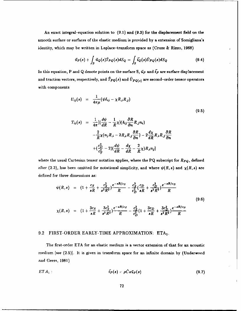
An exact integral-equation solution to (9.1) and (9.3) for the displacement field on the

smooth surface or surfaces of the elastic medium is provided by a extension of Somigliana's

identity, which may be written in Laplace-transform space as (Cruze & Rizzo, 1968)

'Th(s) + L UQ(s)!TpQ(aq)dSQ f Q(.s)U~pQ(s)dSQ (9.4)

In this equation, P and Q denote points on the surface S, lap and (p are surface displacement

and traction vectors, respectively, and TpQ(s) and U]pQ(,) are second-order tensor operators

with components

1

Ui (S) =- .t(k6j -XRRj)

(9.5)

1 di 1 OR R

2 2RiRjOR2)_ d).3nO OR

d2 2+( D- ~ -2(d Rin 3]

T~ d R dR R 'X

where the usual Cartesian tensor notation applies, where the PQ subscript for RpQ, defined

after (2.3), has been omitted for notational simplicity, and where 4(R,s) and x(R,s) are

defined for three dimensions as:

e 2 eaR/csC CI 2__ _______

b(R,s) (1+- + 2R2) c) eR + c2 e

(9.6)(1 3c+ 32 )e-'R/(cs + 3cD 3CD ) -°_e

R -(1 + j_ + _Rx(R, a) _)1e + c h + R

9.2 FIRST-ORDER EARLY-TIME APPROXIMATION: ETA1 .

The first-order ETA for an elastic medium is a vector extension of that for an acoustic

medium [see (2.5)]. It is given in transform space for an infinite domain by (Underwood

and Geers, 1981)

ETA, (p(s) = pCosip(a) (9.7)

72

where C is a second-order tensor that involves the dilatational- and shear-wave speeds

defined in (9.3). For a semi-infinite domain, (9.7) also applies if the DAA boundary is

somewhat removed from the flat traction-free surface of the semi-infinite domain, or if it

intersects the fiat surface at angles equal to or exceeding 900; we restrict ourselves to such

situations.

ETA, is a local approximation, stating that each element of the surface S independently

generates three plane waves, one dilatational and two shear, which propagate normally

outward into the elastic medium. Because it approaches exactness only as s-- oo, it is

singly asymptotic.


FOR A WIOLE-SPACE: LTA'V.

Here, we apply to (9.4) the procedure described in Section 2.3, keeping terms through

So throughout. This yields the standard Somigliana identity.

16P + j UQipQ(0)dSQ f jiQ pQ(0)dSQ, (9.8)

where the tensor components are given by [c.f (9.4) and ( 9.6)]

Uij(O) = 47rp(l- v)R [(3 - 4v)6iRjR,j]

(9.9)

T (0) = 8 - 2 n[(ld - 2v)6ij + 3R,iR,j] - (1 - 2v)(R,inj -Rjn,)T8j(O)-- 8 )(I -n)R

The static relation (9.8) is based on the Green's function for an infinite elastic medium

obtained by Kelvin in 1848. With the spatial-operator definitions

BqQ = j qQpQdSQ

(9.10)

GqQ - fQ[6(P- Q) + ipQ]dSQ

where 6(P - Q) is the Dirac delta-function, (9.8) may be expressed in the form

LTAI': tQ = B- Gilp (9.11)

LTAIV is a non-local, singly asymptotic, quasi-static approximation.

73


FOR A IIALF-SPACE: LTA'.

The first-order LTA for a senii-imfinite space is also a quasi-static approximation ex-

pressed by (9.8), but with T'pQ and UpQ given by expressions corresponding to the half-

space Green's function of Mindlin, 1936, rather than that of Kelvin. These expressions

are constructed by augmenting (9.9) with additional terms (Brebbia,1984). For U, the

augmentation is

UQ = UPQ + U Q (9.12)

in which the components of UjpQ are;

U Kd 8(1 _ v) 2 - (3 - 4v) + (3 - 4v)r, - 2ci 6cir1R/+ R14

[(3 - 4v)r1 4(1 - v)(1 - 2v) + 6 cW 2 = K d r 2R /R 1 + r V

+ ' - R'+r 1'~ + 'R'+rJ9.3

(3 - 4v)rl +4(1 - v)(1 - 2v) 6c:Erl]

U;2 = 'r2 R R' R

U;2= d 1[ (3 -4v)r? + 2ci 1 3r?

/ R/2 \R1

+4r(-v)(1 - 2v) 1 r? (9.13)

,- r' R'(R' + r,)

74(RU2 r'r 2

U;2 U;3

U;3 Kd [1±+ (3 -4v)r2 c ( 12)

74

where (see Figure 25)

ri = z,(p) - z,(Q)

R = (riri)2

ri, = i,(P) - ,(Q')

I (rY)2 (9.14)

S= zi(P)

Kd = 16ir(i - v)IR'

is augmented as

tPQ = tQ +T Q (9.15)

in which the components of t;Q are given by

T,; = fkink (9.16)

where nk is the surface normal (defined as positive going into the medium), and where the

components of or are, with Kt =

Ki r 3(3 - 4v)ir12 - 3cr'(5i - c) 3 rci r]R1 1 13

R1i'

Ktr 2 1 2 3(3 - 4v)0r', - 9ci - 3c 2 30cr7 ]1 2 1 I "" R' 2 R 1

U13 l = Ktr 3 I 2 - 3(3 - 4v)ir - 9ci - 3C _ 30crW'10 " 3 1 -- R '3 I R 2 2R --- 0R 4

K[ (3r, - 4Or') - 3(3 - 4v)rir2(F;21 =- (, 1 ( -2v) I R 2

( I - 2v i - 2vc)_ 30c r r1 2 r I 4R 12 (1 - v)(1 - 2v ) (r 1 _ _ _ -12

R+2 R4 R' + r', R'(R' + r') -R'2

Ktr2 r3 3(3 - 4v)rl 4(1 - v)(1 - 2v) 1 1 3Ocfr0U;3 1 R R2 R 13 + R' + r. (R' + r +' R

75

K t 2')3 , 3(3 - 4v)rlr2 6cr'[(1 - 2v)i - 2vc]31 - (I - v ,( vi - 4vr-) - R,1

3Ocir'2r~ 4R'2(1 - v)(1 - 2v') r 2~ '.2)

R/4 + r' R'(R' + 2,) R

Kt2 [-(-2' 3(3- 4v)r2 6c 2UR + - ( + ( I - 2-)R' + R2 (9.17)

3(3 - 4v)rfr' 6c (n 5 - r2r',O'i22 = RR3 _ 2

1 _,)iI - (1 R 2 )

KR 3 R1 Wf 2 R12

O'2=Kt -3(3 - 4v)r + 6c 1 - 2v +23 2 - -, 2i

o;22 = - [(l - 2v)(5- 4v) 3(3 - 4v)r2 4R'2(1- v)(l1- 2v) 3 r2(3r + r l)

~22 = R'3 R ____2 _ (R' + r;;)2 3 R'-2 (3r + r,)

+ -6c 3c - 3- 2vr' + 5 2 r2)

Ktr 3 3(3 - 4v)r 1 4R' 2 (1 - v)(1 - 2.) ( - (3r + _)

or; 3 2 - -- [ R 2 ( 1 + 2)1 R'2 (R' +

- - R)j

332 - -R (1 - 22)(3 - 33) _ (- ( + ) + I R( -+ r')

R' 3 [ '2 (R' + r')) 2 (kRo 2 R ++ - ~~ +r12, + )

K6 ['' 3(3-4)rr i 6( (12 5 r'r

U133 : [,-- 1 v)rl~ .. .. .

Y'2 R12 /

U 3 L .Kt r2 2v)(3 - 4v) - 3(3- 4v)r _ 4R' 2(1 _ V)(1 - 2v) 1 r3'(3r + r')R13 R (R' + r)2 k R)2+ )

+ c- (1- 2v)r' + W r ,R2('+r-L 2 3(3 - 4v)r/ 2 (1-v( ,) r(r+v c r

o';2 = -i - (1-, 3( -- l 4vr2R ,3 2v ( -1 -v) -, R -12 2 I - ( '+ i -2-) 1 --2

36 (R' + r )2 + r + r,)+ 6 c ( - v~f, U 0

R'(R +76)

Ktr 3 [ 3(3-4v)r a 4R' 2(1-v)(1- 2v) r32(3r+r'0'333 = _j1_ (1 - 2v)(5 -4v)- Rr2 r ' -)2 3- + r',

6c (3c- (3 - 2v)r' + 5ir 12R' 2 I ,2 3)

In operator notation, LTAI for the semi-infinite domain appears the same as that for the

infinite domain, given by (9.11).

9.5 FIRST-ORDER DOUBLY ASYMPTOTIC APPROXIMATIONS FOR

WHOLE- AND HALF-SPACES: DAA 1 .

Because the only differences between the first-order early- and late-time approxima-

tions for infinite and semi-infinite domains reside in the operators TpQ and U]PQ, we can

formally develop first-order DAA's for the two domains simultaneously. We will use the

method of operator matching for this purpose. The appropriate trial equation is

[sP1 + Polirp(s) = ia(S) (9.18)

where the spatial operators ,A and A are not functions of s.

For s- 0 we write (9.18) as

[ 0 + 0()]PIp(s) = iQ(s) (9.19)

and match with (9.11) as s--* 0, which yields Po =h - '. This the asymptotic match for

the static limit. For s-+ oo we divide (9.18) through by s to get

[Pi + 0(s')gp(s) =S-Q(8) (9.20)

Now we match with (9.7) as s---. o to give A = pC. Introducing these results into (9.18),

we obtain, in transform space,

DAAi(s)= [p10,8 + 3-1B ] trp(s) (9.21)


DAAI(t): FQ(t) = pCp(t) + B-Gtip(t) (9.22)

Note that the DAA 1 for elastic domains is not spatially local, because of the late-time

approximation term.

77

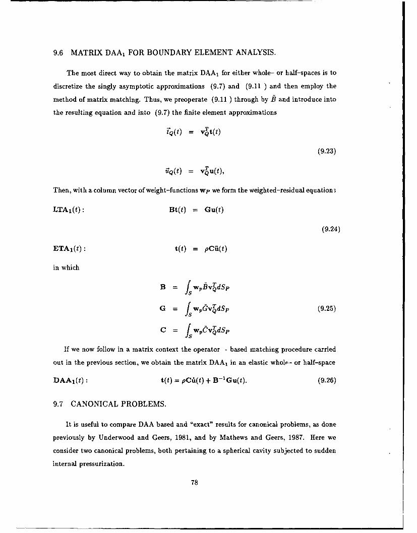
9.6 MATRIX DAA 1 FOR BOUNDARY ELEMENT ANALYSIS.

The most direct way to obtain the matrix DAA 1 for either whole- or half-spaces is to

discretize the singly asymptotic approximations (9.7) and (9.11 ) and then employ the

method of matrix matching. Thus, we preoperate (9.11 ) through by t and introduce into

the resulting equation and into (9.7) the finite element approximations

tQ(t) = v~t(t)

(9.23)

t q(t) = v u(t),

Then, with a column vector of weight-functions wp we form the weighted-residual equation;

LTA 1(t): Bt(t) = Gu(t)

(9.24)

ETA 1(t): t(t) = pCii(t)

in which

B = fsW,,3v~dSp

G = fLWPOVdSp (9.25)

C = fsWvO dSp

If we now follow in a matrix context the operator - based matching procedure carried

out in the previous section, we obtain the matrix DAA 1 in an elastic wholp- or half-space

DAA 1(t) : t(t) = pCii(t) + B 1 Gu(t). (9.26)

9.7 CANONICAL PROBLEMS.

It is useful to compare DAA based and "exact" results for canonical problems, as done

previously by Underwood and Geers, 1981, and by Mathews and Geers, 1987. Here we

consider two canonical problems, both pertaining to a spherical cavity subjected to sudden

internal pressurization.

78

The first problem is a spherical cavity embedded in an infinite elastic medium and excited

by an internal step pressure. This problem possesses radial symmetry, and has a well-known

analyticd solution (Timoshenko & Goodier 1970). With a as the cavity radius and Po as

the pressure magnitude, the radial displacement of the cavity is given by

u(t) =_foa {ae-(cos ast + 1 sin as't)

-ae-a( - sin as't + cos as't) (9.27)

+1 - e -t(cosas't + 1 sin as't)}.

where

= CD(l - 2v)

a(1 - v)

(9.28)

st =

V1 - 2v

The corresponding analytical DAA solution is simply

UDAA P1a 1- e - 4 t /a CD) (9.29)

In order to generate numerical DAA solutions, a dynamic boundary element program has

been built that is based upon the program constructed by Mathews (Mathews and Geers,

1987). The program uses eight node quadratic quadrilaterals for spatial discretization and

the trapezoidal rule for time integration. For the present problem, the boundary-element

model for the cavity boundary consists of 24 eight node elements over the entire spherical

surface. The analytical exact, analytical DAA1 , and numerical DAA1 solutions are shown

in Figure 26 for the parameters p = 1.00, ft = 1/6, v = 1/4, a = 1, and P0 = 1. The

analytical DAA1 and numerical DAA1 solutions are seen to be almost identical, and the

DAAI solutions agree well with the analytical exact solution at both early and late times.

As previously observed by Underwood and Geers, 1987, the DAA1 solutions do not exhibit

the response overshoot seen in the exact solution. This is characteristic of solutions to first-

order differential equations like (9.26). A second-order DAA is capable of accommodating

such overshoot.

The second problem is a spherical cavity embedded in a semi-infinite elastic medium and

excited by an internal step pressure. This problem does not posses radial symmetry, and

79

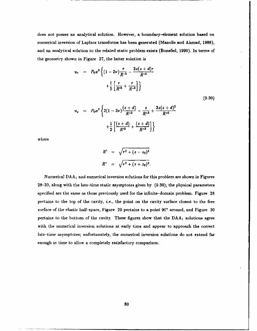
does not posses an analytical solution. However, a boundary-element solution based on

numerical inversion of Laplace transforms has been generated (Manolis and Ahmad, 1988),

and an analytical solution to the related static problem exists (Bonefed, 1990). In terms of

the geometry shown in Figure 27, the latter solution is

Sr 3z(z + d)ru. = oa 1 R -2v)- 3 R s

(9.30)

=Z Poa 3{12 (1 -2 ) (z +d) - ~+ R5z d-Uz(- -

±( +d) +(z +d)]}

where

= Vr 2 + (z - zO) 2

= /r 2 + (z + zo) 2.

Numerical DAA, and numerical inversion solutions for this problem are shown in Figures

28-30, along with the late-time static asymptotes given by (9.30); the physical parameters

specified are the same as those previously used for the infinite-domain problem. Figure 28

pertains to the top of the cavity, i.e., the point on the cavity surface closest to the free

surface of the elastic half-space, Figure 29 pertains to a point 900 around, and Figure 30

pertains to the bottom of the cavity. These figures show that the DAA1 solutions agree

with the numerical inversion solutions at early time and appear to approach the correct

late-time asymptotes; unfortunately, the numerical inversion solutions do not extend far

enough in time to allow a completely satisfactory comparison.

80

SECTION 10

CONCLUSION

This report documents the formulation and evaluation of new doubly asymptotic

approximations for simplifying the analysis of transient medium-structure interaction problems.

More specifically,

1. The formulation of first- and second-order DAA's for an external acoustic medium has been

systematized; finite-element discretization has been introduced to configure the operator-based

formulation for boundary-element solution.

2. First- and second-order DAA's for an internal acoustic medium have been systematically

formulated on an operator basis; finite-element discretization has been introduced to configure

the formulation for boundary-element solution.

3. The canonical problem of a spherical shell filled with an acoustic fluid, submerged in an

acoustic medium, and excited by a plane step-wave has been solved by modal analysis; special

techniques have been developed and applied to achieve satisfactory convergence.

4. Extensive numerical results for the canonical problem have been generated for exact, DAA,

and DAA 2 treatments of the internal and external fluid-structure interactions; the numerical

results have been compared to assess DAA accuracy.

5. The formulation of the first-order DAA for an infinite elastic medium has been systematized;

finite-element discretization has been implemented to configure the operator-based formulation

for boundary-element solution.

6. The first-order DAA for a semi-infinite elastic medium has been systematically formulated

81

on an operator basis; finite-element discretization has been implemented to configure the

formulation for boundary-element solution.

7. Boundary-element DAA results for suddenly pressurized spherical cavities embedded in

infinite and semi-infinite elastic media have been generated; the DAA results have been

compared with corresponding results by other investigators.

The principal conclusions reached during this study are:

1. First-order DAA's are marginally satisfactory for approximating transient medium-structure

interactions involving external and internal acoustic domains and external elastic domains.

2. Second-order DAA's are highly satisfactory for treating external acoustic domains; they are

satisfactory for treating internal acoustic domains.

3. The second-order DAA for an internal acoustic medium is sufficiently accurate to warrant

early implementation in production codes for underwater shock analysis.

4. Second-order DAA's are needed for treating infinite and semi-infinite elastic media; the

techniques used herein to formulate second-order DAA's for an acoustic medium may be applied

to an elastic medium as well.

5. Further DAA development is desirable in order to obtain approximations of higher accuracy

and broader application.

82

SECTION 11

LIST OF REFERENCES

1. Apostol, T.M., 1957, "Mathematical Analysis: A Modem Approach to AdvancedCalculus", Addison-Wesley Pub. Co..

2. Abramowitz, M. and Stegun, I.A., 1964, "Handbook of Mathematical Functions", NBSAppl. Math. Ser. 55 (U.S. Dept. of Commerce, Washington, DC).

3. Atkash, R., et al., 1987, "Developments for the EPSA Computer Code", DNA-TR-87-155,Defense Nuclear Agency, Washington, DC.

4. Baker, B.B. and Copson, E.T., 1939, "The Mathematical Theory of Huygen's Principle",Clarendon Press, Oxford.

5. Bannerjee, P.K. and Butterfield, R., 1981, "Boundary Element Methods in EnginneringScience", McGraw-Hill Book Company (UK) Limited, London.

6. Bonefed, M., 1990, "Axisymmetric Deformation of a Thermo-poro-elastic Halfspace;Inflation of a Magma Chamber", Geophys. T. Inter, Vol. 103, pp. 289-299.

7. Chertock, G., 1971, "Integral Equation Methods in Sound Radiation and Scattering fromArbitrary Surfaces", Rep. No. 3538, Naval Ship Research and Development Center, Carderock,MD.

8. Cruse, T.A. and Rizzo, F.T., 1968, "A Direct Formulation and Numerical Solution of theGeneral Transient Elastodynamic Problem", Math. Analysis & Appl., Vol. 22, pp. 244-259.

9. DeRuntz, J.A. and Geers, T.L., 1978, "Added Mass Computation by the Boundary IntegralMethod", Int. J. Numer. Meth. Eng., Vol. 12, pp. 531-549.

10. DeRuntz, J.A., Geers, T.L. and Felippa, C.A., 1980, "The Underwater Shock AnalysisCode (USA-Version 3)", DNA 5615F, Defense Nuclear Agency, Washington, DC.

11. DeRuntz, J.A., and Brogan, F.A., 1980, "Underwater Shock Analysis of NonlinearStructures, A Reference Manual for the USA-STAGS Code (Version 3)", DNA 5545F, DefenseNuclear Agency, Washington, DC.

12. Felippa, C.A., 1980, "A Family of Early-Time Approximations for Fluid StructureInteraction", J. Appl. Mech., Vol. 47, pp. 703-708.

83

13. Felippa, C.A., 1980a, "Top-down Derivation of Doubly Asymptotic Approximations forStructure-fluid Interaction Analysis", in "Innovative Numerical Analysis for the EngineeringSciences", edited by R.P. Shaw et al., U.P. of Virginia, Charlottesville, pp 79-88.

14. Friedlander, F.G., 1958, "Sound Pulses", Cambridge University Press, Cambridge.

15. Geers, T.L., 1969, "Excitation of an Elastic Cylindrical Shell by a Transient AcousticWave", J. Appl. Mech., Vol. 36, pp. 459-469.

16. Geers, T.L., 1971, "Residual Potential and Approximate Methods for Three-dimensionalFluid-structure Interaction Problems", J. Acoust. Soc. Am., Vol. 49, pp. 1505-1510.

17. Geers, T.L., 1972, "Scattering of a Transient Acoustic Wave by an Elastic CylindricalShell", J. Acoust. Soc. Am., Vol. 51, pp. 1640-1651.

18. Geers, T.L., 1974, "Shock Response Analysis of Submerged Structures", Shock andVibration Bulletin, Vol. 44, Supp. 3, pp. 17-32.

19. Geers, T.L., 1975, "Transient Response Analysis of Submerged Structures", in "FiniteElement Analysis of Transient Nonlinear Structural Behavior', edited by T. Belytschko and T.L.Geers, AMD-vol. 14, ASME, New York, pp. 59-84.

20. Geers, T.L., 1976, "Submerged Structure Survivability (U)", Proc. AIAA 3rd JointStrategic Sciences Meeting, San Diego, CA.

21. Geers, T.L., 1978, "Doubly Asymptotic Approximation for Transient Motions ofSubmerged Structures", J. Acoust. Soc. Am., Vol. 64, pp. 1500-1508.

22. Geers, T.L. and Felippa, C.A., 1983, "Doubly Asymptotic Approximations for VibrationAnalysis of Submerged Structures", J. Acoust. Soc. Am., Vol. 73, pp. 1152-1159.

23. Geers, T.L. and Ruzicka, G.C., 1984, "Finite-Element / Boundary-Element Analysis ofMultiple Structures Excited by Transient Acoustic Waves", in "Numerical Methods for Transientand Coupled Problems", edited by R.W. Lewis, etal. Pineridge Press, Swansea, UK, pp. 150-162.

24. Geers, T.L. and Zhang, P., 1988, "Doubly Asymptotic Approximations forElectromagnetic Scattering Problems", in "Boundary Element Methods in Applied Mechanics",edited by M. Tanaka and T.A. Cruse, Pergamon Press, Oxford, pp. 357-369.

25. Geers, T.L. and Zhang, P., 1989, "Response of a Fluid-filled Spherical Shell in an InfiniteFluid Medium to a Transient Acoustic Wave", presented at the 118th Meeting of Acoust. Soc.Am., St. Louis, Missouri.

84

26. Geers, T.L., 1990, "Doubly Asymptotic Approximations for a spherical Acoustic Domain",Appendix A to a DNA report submitted in draft form by NKF Engineering, Inc. in November1990.

27. Huang, H., 1969, "Transient Interaction of Plane Waves with a Spherical Elastic Shell",J. Acoust. Soc. Am., Vol. 45, pp. 661-670.

28. Huang, H. 1979, "Transient Response of Two Fluid-coupled Spherical Elastic Shells toan Incident Pressure Pulse", J. Acoust. Soc. Am., Vol. 65, pp. 881-887.

29. Hughes, T.J.R. and Hinton, E., 1986, "Finite Element Methods for Plate and ShellStructures", Pineridge Press International, Swansea, U.K.

30. Junger, M.C. and Feit, D. 1972, "Sound, Structures, and Their Interaction", (MIT press,Cambridge, MA).

31. Lamb, H.S., 1945, "Hydrodynamics", Dover Publications, New York.

32. Mathews, I.C., and Geers, T.L., 1987," A Doubly Asymptotic, Non-Reflecting Boundaryfor Ground-Shock Analysis", J. Appl. Mech., Vol. 54, pp. 489-497.

33. Milne-Thomson, L.M., 1960, "Theoretical Hydrodynamics", Macmillan, New York.

34. Morse, P.M. and Ingard, K.U., 1968, "Theoretical Acoustics", McGraw-Hill, New York.

35. Neilson, H.C. et al., 1981, "Transient Response of a Submerged, Fluid-Coupled, Double-Walled Shell Structure to a Pressure Pulse", J. Acoust. Soc. Am., Vol. 70, pp. 1776-1782.

36. Nicolas-Vullierme, B., 1989, "A Contribution to Doubly Asymptotic Approximations: AnOperator Top-down Approach", Numerical Techniques in Acoustic adiation, NCA-Vol.6, ASME,

New York, pp. 7-13.

37. Pierce, A.D., 1981, "Acoustics: an Introduction to its Physical Principles andApplications", McGraw-Hill Book Co., New York.

38. Ranlet, D., et al., 1977, "Elastic Response of Submerged Shells with Internally AttachedStructures to Shock Loading", Int. J. Computers and Structures, Vol. 7, pp. 355-364.

39. Sobolev, S.L., 1964, "Partial Differential Equations of Mathematical Physics", PergamonPress, London.

40. Tang, S. and Yen, D., 1970, "Interaction of a Plane Acoustic Wave with an ElasticSpherical Shell", J. Acoust. Soc. Am. 47, pp. 1325-1333.

85

41. Thomson, S.W., 1848, "Math and Phys. Papers", vol. 1, pp. 97.

42. Timoshenko, S.P. and Goodier, T.N., 1970, "Theory of Elasticity", McGraw-Hill.

43. Underwood, P.G., and Geers, T.L., 1981, "Doubly Asymptotic, Boundary-ElementAnalysis of Dynamic Soil-Structure Interaction", Int. J. Solids and Structures, Vol. 17, pp. 687-697.

44. Vasudevan, R., and Ranlet, D., 1982, "Submerged Shock Response of a Linear ElasticShell of Revolution Containing Internal Structure-Users Manual for the ELSHOK Code", DNA-TR-81-184, Defense Nuclear Agency, Washington, DC.

86

APPENDIX

FIGURES

87

-zINFINITE FLUID

Ie, Ce

>w

z

FL Iz P

Figure 1. Geometry of the spherical shell problem.

0.8-

0.4-

0.6-

0 1 2 3 4 5 a 7a

standar pata umto*C3N=Ceiosmainoe oe3 -hruhS;S-5 =prta sm ao avrmds0 hog )

- - - 88

9 1. -- --

5..-100-.8

0.0

-.0.5

0 2

nondimensional time t.

Figure 3. Incident-wave pressure histories produced by standardpartial summation (PSN = partial summation overmodes 0 through N, e = r-s error over 0 :5 t :5 2).

~1.0 -- - - - - -

CS -... O~-.13

C 35.-. -. 13

-.0.5 _

0 123

nondimenSlonal time L.

Figure 4. Incident-wave pressure histories produced by modifiedCeshro Summation (CS 3-N = Ceshro summation overmodes 3 through N, e = in-s error over 0 5 t 5 2).

89

0.18

0.16

LI0.12-/4 ,

mr 0.104r., ----'

0.08

modified Cealro summation0.06- -- standard partial summation

180 160 140 120 100 so 6'0 410 20 0

meridional coordinate 0

Figure 5. Mean-square error in modal summations forincident pressure histories over 0 <5 t 2 (N 8).

2.0-

n-0-8" "" n-0-5

-- 0.5-

0

0.00 3 4 5 a 8 9 0

nondimensional time t

Figure 6. External- and internal-surface pressure histories by modified

Cesi sunmation (CS) for a steel shell at 0 = i 8.

90

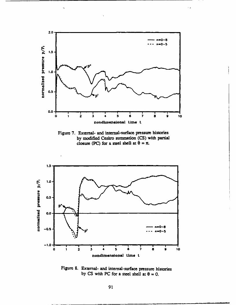
2.0-

-n-0-8

--- n=0-5

0. 1.0

a. 0.5-

0.


Figure 7. External- and internal-surface pressure historiesby modified Ces~ro summation (CS) with partialclosure (PC) for a steel shell at e 7-

0: 1.0-

0.5-G6

C -05 ,--- n:0-5


Figure, 8. External- and internal-surface pressure histories

by CS with PC for a steel shell at 0 =0.

91

1.25

4 1.00

.2 0.75

*~0.50-

--- n-0-50.00

-0.25 10 1 2 ,3 4 5 6 7 a 1


Figure 9. Radial shell-velocity histories by CS with PCfor a steel shell at 0) =c and 0 =0.

2.0*

- n-0-15

~1.5

fluid-filled shell

Q.1.0

S. 0.5

0 1 2 3 4 5 6 7 8 9 10

nondimensional time t.

Figure 10. External-surface pressure histories at 0 nfor a fluid-filled shell and an empty shell.

92

1.50

1.25cc fluid-filled shellIN

1.00

0.75v

v 0.50 empty shell

E 0.25 - n-0-80 --- n-0-5C

0.00

-0.250 2 4 5 6 7 a 9 10


Figure 11. External-surface pressure histories at 0 = 7r/2for a fluid-filed shell and an empty shell

1.5-

*u empty shell1 .0-

2.0L

0 %t%fluid-filled shell -- n-0-8;= --- n-0-5

0.0

''.

0 2 3 4 5 6 7 10

nondimensionai time t

Figure 12. External-surface pressure histories at O 0for a fluid-filled shell and an empty shell.

93

3.0-

2.0-

*1.5

N1.0

0.

S0.5

0 1 2 .3 4 5 6 7 a 9 10


Figure 13. Radial shell-velocity histories at 0 = 7for a fluid-filled shell and an empty shell.

4.

-n-0-8

... n-0-5

e3empty shell

0 2

0fli -ile h l

0-

0 1 2 3 4 5 6 7 5 9 1o

nondimensional time L

Figure 14. Radial shell-velocity histories at 9=0for a fluid-filled shell and an empty shell.

94

1.2-

.-

S0.6-

0.4

N 0.6-

0 0.0

2..

OA0

IX

.0- -- - - - - - -

0.0~

~ 195

1.0

- exoct

cc 0.8

0.6 4

0. 4- - -

0 0 0.2

0.0 , , ,

0 1 2 3 4 5 6 7 8 9 10


Figure 17. Exact, DAA1 and DAA% internal-surfacepressure histories at 0 = x for a steel sheel.

1.00

0.75* 0.70L.

L00. 0.50

Fiue1.Eat-AIadDAetr-.,

- eoct

'0.25 . A

sufc prsuehsoie t0=w20 2 3 4 5 6 7 9 10nondimensional time t

Figure 18. Exact, DAN 1 and DAA2 external-surface pressue histories at 0 --= 2

96

0.8

I 0.

=-In

Fibr 19 Exat, AA 1 nd AA 2 m eract

0.-

A. Ai0.2 -DAAe

o2 / -- DAA

0 0.0

-0.20 1 2 3 4 5 6 7 9 10


Figure 19. Exact, DAA, and DAA 2 internal-surface pressure histories at 0 = 2.

9.5

0.00 - /D* -

.00

61 0.7 3 7 a 9

Fiur 2.ExcDAan A2etml

surac prsuehsore t0 0

I97

1.00-

0.75-

-~0.50-

:3 0.5

S0.005

*4 -0.25-

1. 0.50 - exact0 -DAA.

-0.*75 -DAA*

-1.00I I0 1 2 3 4 5 6 7 8 9 10

nondimerxsional time t.

]Figure 21. Examt DAA, and DAA 2 internal-surface pressure histories at 0 0.

1.4

0.4

0

0.2

nondlmensional trne t

]Figure 22. Exact, DAA, and DAA 2 radialshell-velocity histories at9

98

1.2-

1.0

>% 0.8-

0> 0.6-

c 0.4-EL. - exact0

- AA,0 .2 D A..

0.0

0 1 2 3 4 5 6 7 8 9 10

nondimensionel time t

Figure 23. Exact, DAA, and DAA2 circumferentialshell-velocity histories at 0 = n/2.

1.50~

1.25 ,1 .

1.00 %%*" .s° ],I / "- \.- / -' "

I I / I, -\, ' I

:/ I I ... \ , -g

IN!

" 0.75 . -.0.0 ".N I -exact

0.25 , - ,

C0.00.

-0.25~

0 1 2 3 4 5 6 7 8 9 10nondimensional time t

Figure 24. Exact, DAA, and DAA 2 radial shell-velocity histories at 8 = 0.

99

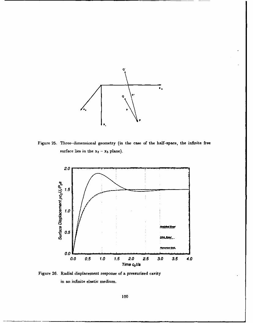
xx

P

x

Figure 25. Three-dimensional geometry (in the case of the half-space, the infinite free

surface lies in the x2 - X3 plane).

2.0

1.0

S0.5

0.00.0 0.5 1.0 1.5 2.0 2.5 3.0 3.5 4.0

Time cDfta

Figure 26. Radial displacement response of a pressurized cavity

in an infinite elastic medium.

100

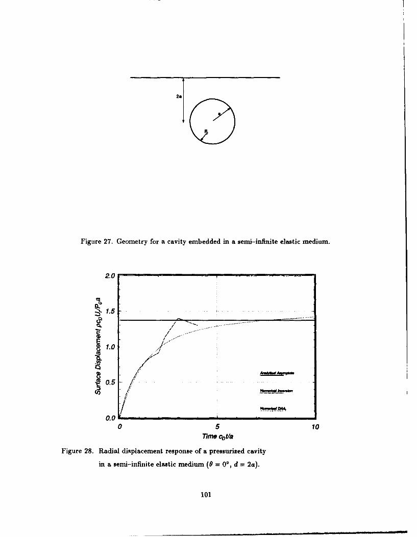
2a

Figure 27. Geometry for a cavity embedded in a semi-infinite elastic medium.

2.0 - -

-1.5 7--Q~

............................

~1.0 .

JIM0.5 /

0.00 5 10

rIMe C,,ta

Figure 28. Radial displacement response of a pressurized cavity

in a semi-infinite elastic medium (0 = 00, d = 2a).

101

2.0 71..... ..

.5

0 5 1

.0

1.5

Q.

S0.5 /M~q

0.00 5 10

TIMe C~ta

Figuire 29. Radial displacement response of a pressurized cavity

in a semi-infinite elastic medium (9 = 90, d = 2a).

010

DISTRIBUTION LISTDNA-TR-91-69

DEPARTMENT OF DEFENSE DEPARTMENT OF THE NAVY

ASSISTANT TO THE SECRETARY OF DEFENSE DAVID TAYLOR RESEARCH CENTERATTN: EXECUTIVE ASSISTANT ATTN: CODE 172

ATTN: CODE 173DEFENSE INTELLIGENCE AGENCY ATTN: CODE 1740

ATTN: DB-6E1 ATTN: CODE 1750ATTN: OGA-4B2 ATTN: CODE 1770

ATTN: CODE 2740DEFENSE NUCLEAR AGENCY

ATTN: OPNS DEPARTMENT OF THE NAVYATTN: SPSD ATTN: SEA-08ATTN: SPWE ATTN: SEA-423

2 CYS ATTN: TITL ATTN: SEA-511ATTN: SEA-55X1

DEFENSE TECHNICAL INFORMATION CENTER ATTN: SEA-55Y2 CYS ATTN: DTIC/FDAB

MARINE CORPSFIELD COMMAND DEFENSE NUCLEAR AGENCY ATTN: CODE POR-21

ATTN: FCPRNAVAL COASTAL SYSTEMS CENTER

FIELD COMMAND DEFENSE NUCLEAR AGENCY ATTN: CODE 7410ATTN: FCNV

NAVAL DAMAGE CONTROL TRAINING CENTERFIELD COMMAND DEFENSE NUCLEAR AGENCY ATTN: COMMANDING OFFICER

ATTN: FCNMNAVAL ELECTRONICS ENGRG ACTVY, PACIFIC

THE JOINT STAFF ATTN: CODE 250ATTN: JKC DNA REPATTN: JKCS NAVAL EXPLOSIVE ORD DISPOSAL TECHNOLOGY CENTER

DEPARTMENT OF THE ARMY ATTN: CODE 90 J PETROUSKY

NAVAL POSTGRADUATE SCHOOLDEP CH OF STAFF FOR OPS & PLANS ATTN: CODE 1424 LIBRARY

ATN: DAMO-SWNHARRY DIAMOND LABORATORIES NAVAL RESEARCH LABORATORY

ATTN: SLCIS-IM-TL ATTN: CODE2627NAVAL SURFACE WARFARE CENTER

U S ARMY CORPS OF ENGINEERS ATTN: CODE H21ATTN: CERD-L ATTN: CODE R14

U S ARMY ENGR WATERWAYS EXPER STATION ATTN: CODE R15ATTN: CEWES J K INGRAM NAVAL WEAPONS CENTERATTN: CEWES-SD DR J G JACKSON JR ATTN: CODE 3263 J BOWENATTN: J ZELASKO CEWES-SD-RATTN: R WHALIN CEWES-ZT NAVAL WEAPONS EVALUATION FACILITYATTN: RESEARCH LIBRARY ATTN: CLASSIFIED LIBRARY

U S ARMY NUCLEAR & CHEMICAL AGENCY NEW LONDON LABORATORYATTN: MONA-NU OR D BASH ATTN: TECH LIBRARY

U S ARMY STRATEGIC DEFENSE COMMAND OFFICE OF CHIEF OF NAVAL OPERATIONSATTN: CSSD.SA-EV ATTN: NOP 091ATTN: CSSD-SL ATTN: NOP 223

ATTN: NOP 225U S ARMY WAR COLLEGE ATTN: NOP 37ATTN: LIBRARY ATTN: NOP 605D5

USA SURVIVABILITY MANAGMENT OFFICE ATTN: NOP 957EATTN: SLCSM-SE J BRAND ATTN: OP 03EG

ATTN: OP 21

ATTN: OP 654ATTN: OP 73

Dist-1

DNA-TR-91-69 (DL CONTINUED)

OFFICE OF NAVAL RESEARCH KAMAN SCIENCES CORPATTN: CODE 1132SM ATTN: LIBRARYATTN: CODE 23

KAMAN SCIENCES CORPDEPARTMENT OF THE AIR FORCE ATTN: DASIAC

ATTN: E CONRADAIR FORCE INSTITUTE OF TECHNOLOGY/EN

ATTN: COMMANDER KAMAN SCIENCES CORPORATIONATTN: DASIAC

HQ USAF/CCNATTN: AFCCN KARAGOZIAN AND CASE

ATTN: J KARAGOZIANDEPARTMENT OF ENERGY

LOCKHEED MISSILES & SPACE CO, INCLAWRENCE LIVERMORE NATIONAL LAB ATTN: PHILIP UNDERWOOD

ATTN: D MAGNOLILOCKHEED MISSILES & SPACE CO. INC

LOS ALAMOS NATIONAL LABORATORY ATTN: TECH INFO CTRATTN: REPORT LIBRARYATTN: TECH LIBRARY PACIFIC-SIERRA RESEARCH CORP

ATTN: H BRODEMARTIN MARIETTA ENERGY SYSTEMS INC

ATTN: DR C V CHESTER S-CUBEDATTN: K D PYATT JR

SANDIA NATIONAL LABORATORIES ATN: R SEDGEWICKATTN: TECH LIB 3141

SCIENCE APPLICATIONS INTL CORPU.S. DEPARTMENT OF ENERGY ATTN: TECHNICAL REPORT SYSTEMOFFICE OF MILITARY APPLICATIONS

ATTN: OMA/DP-252 MAJ D WADE TELEDYNE BROWN ENGINEERINGATTN: J RAVENSCRAFT

OTHER GOVERNMENTTHE TITAN CORPORATION

CENTRAL INTELLIGENCE AGENCY ATTN: LIBRARYATTN: OSWR/NED ATTN: S SCHUSTER

DEPARTMENT OF DEFENSE CONTRACTORS UNIVERSITY OF COLORADO2 CYS ATTN: B A LEWIS

AN ANALYSIS & TECHNOLOGY COMPANY 2 CYS ATTN: P ZHANGATTN: V GODINO 2 CYS ATTN: T L GEERS

APPLIED RESEARCH ASSOCIATES, INC WEIDLINGER ASSOC, INCATTN: R FRANK ATTN: H LEVINE

CALIFORNIA INSTITUTE OF TECHNOLOGY WEIDLINGER ASSOCIATES, INCATTN: T AHRENS ATTN: T DEEVY

CALIFORNIA RESEARCH & TECHNOLOGY, INC WEIDLINGER ASSOCIATES, INCATTN: J THOMSEN ATTN: M BARONATTN: K KREYENHAGEN

COLUMBIA UNIVERSITY WESTINGHOUSE ELECTRIC CORP

ATTN: F DIMAGGIO ATTN: D BOLTON

Dist-2

advanced daa methods dtic thomas l. geers peizhen …

Documents