advanced data structures and algorithms - old …€¦ · · 2013-09-09page 2 fall 2013 cs 361 -...
TRANSCRIPT
Advanced Data Structures and Algorithms
�CS 361 - Fall 2013 �
Tamer Nadeem �Dept. of Computer Science�
Lec. #02: Introduction to Algorithms
Page 2 Fall 2013 CS 361 - Advanced Data Structures and Algorithms
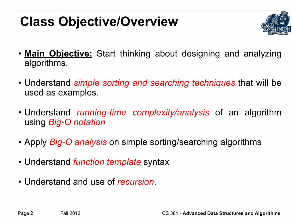
Class Objective/Overview
• Main Objective: Start thinking about designing and analyzing algorithms.
• Understand simple sorting and searching techniques that will be used as examples.
• Understand running-time complexity/analysis of an algorithm using Big-O notation
• Apply Big-O analysis on simple sorting/searching algorithms
• Understand function template syntax
• Understand and use of recursion.
Page 3 Fall 2013 CS 361 - Advanced Data Structures and Algorithms
Simple Sorting & Searching
Techniques
Page 4 Fall 2013 CS 361 - Advanced Data Structures and Algorithms
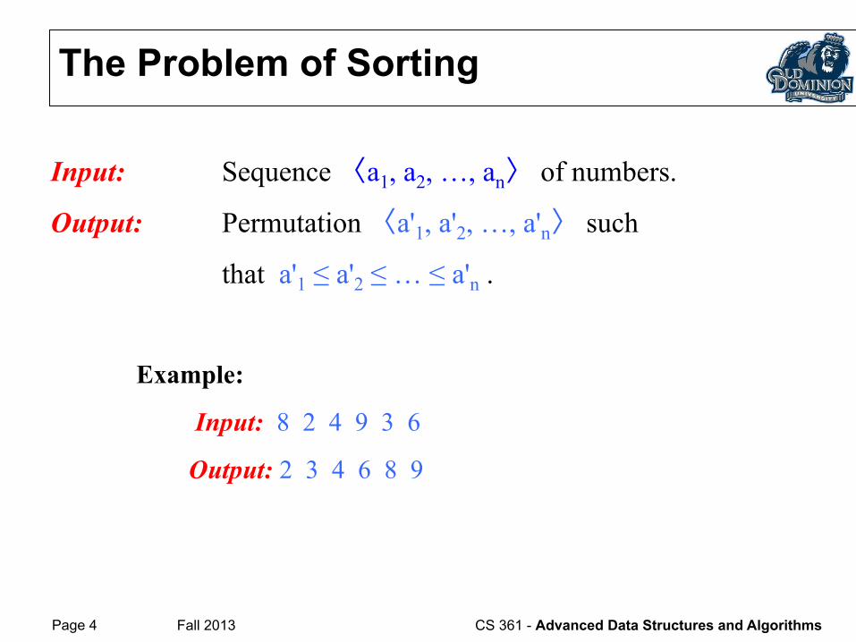
Input: Sequence 〈a1, a2, …, an〉 of numbers.
Output: Permutation 〈a'1, a'2, …, a'n〉 such
that a'1 ≤ a'2 ≤ … ≤ a'n .
Example:
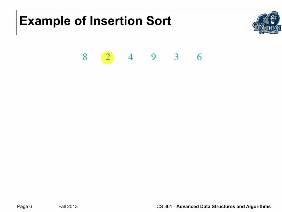
Input: 8 2 4 9 3 6
Output: 2 3 4 6 8 9
The Problem of Sorting
Page 5 Fall 2013 CS 361 - Advanced Data Structures and Algorithms
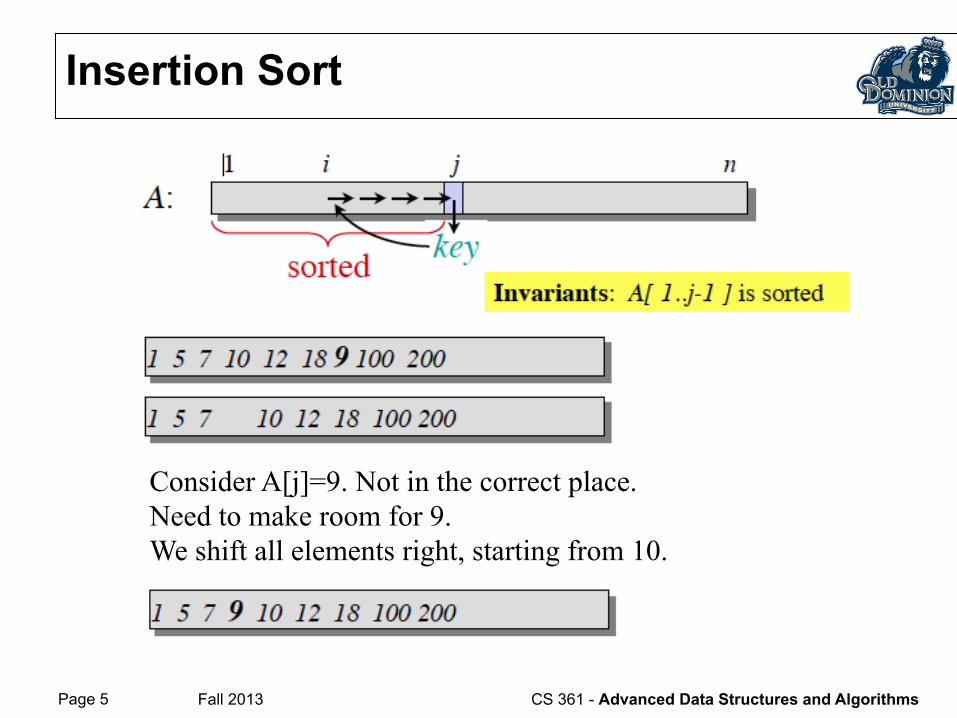
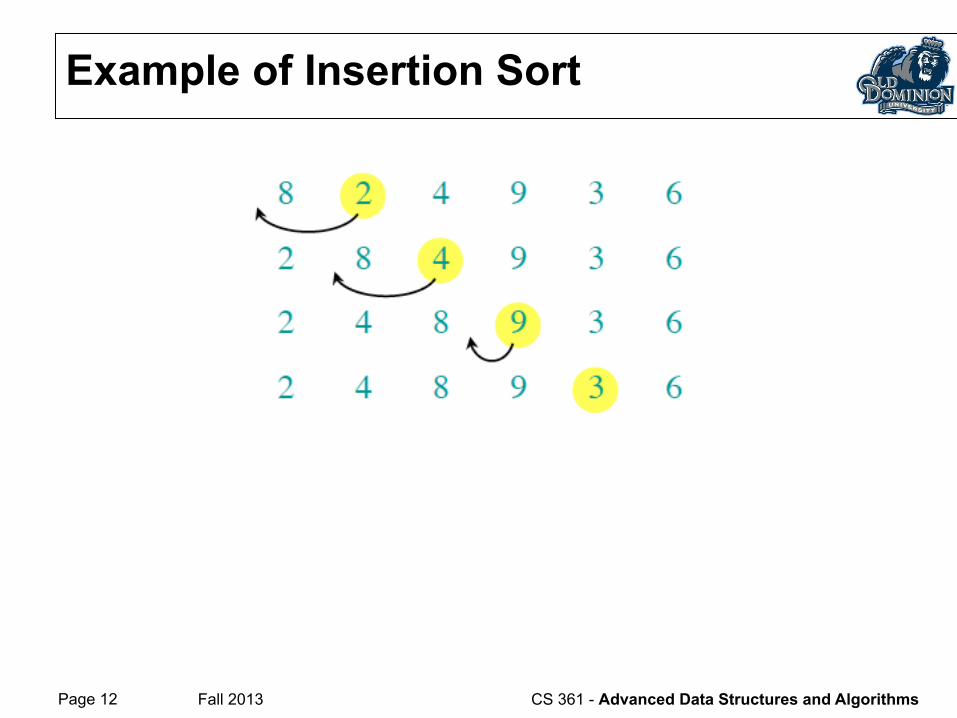
Insertion Sort
Consider A[j]=9. Not in the correct place. Need to make room for 9. We shift all elements right, starting from 10.
Page 6 Fall 2013 CS 361 - Advanced Data Structures and Algorithms
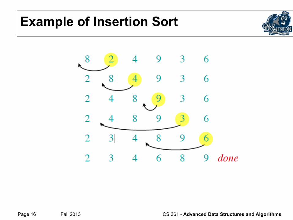
Example of Insertion Sort

Page 7 Fall 2013 CS 361 - Advanced Data Structures and Algorithms
Example of Insertion Sort

Page 8 Fall 2013 CS 361 - Advanced Data Structures and Algorithms
Example of Insertion Sort
Page 9 Fall 2013 CS 361 - Advanced Data Structures and Algorithms
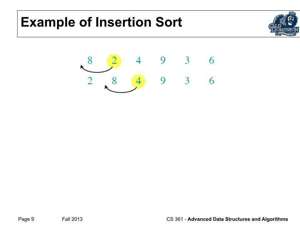
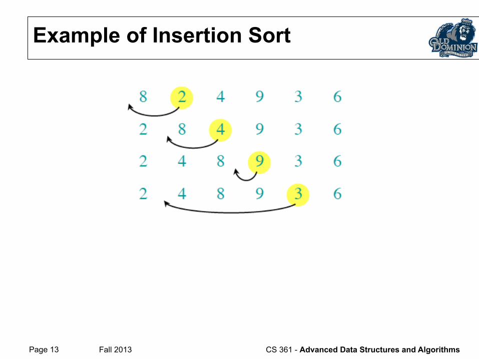
Example of Insertion Sort

Page 10 Fall 2013 CS 361 - Advanced Data Structures and Algorithms
Example of Insertion Sort
Page 11 Fall 2013 CS 361 - Advanced Data Structures and Algorithms
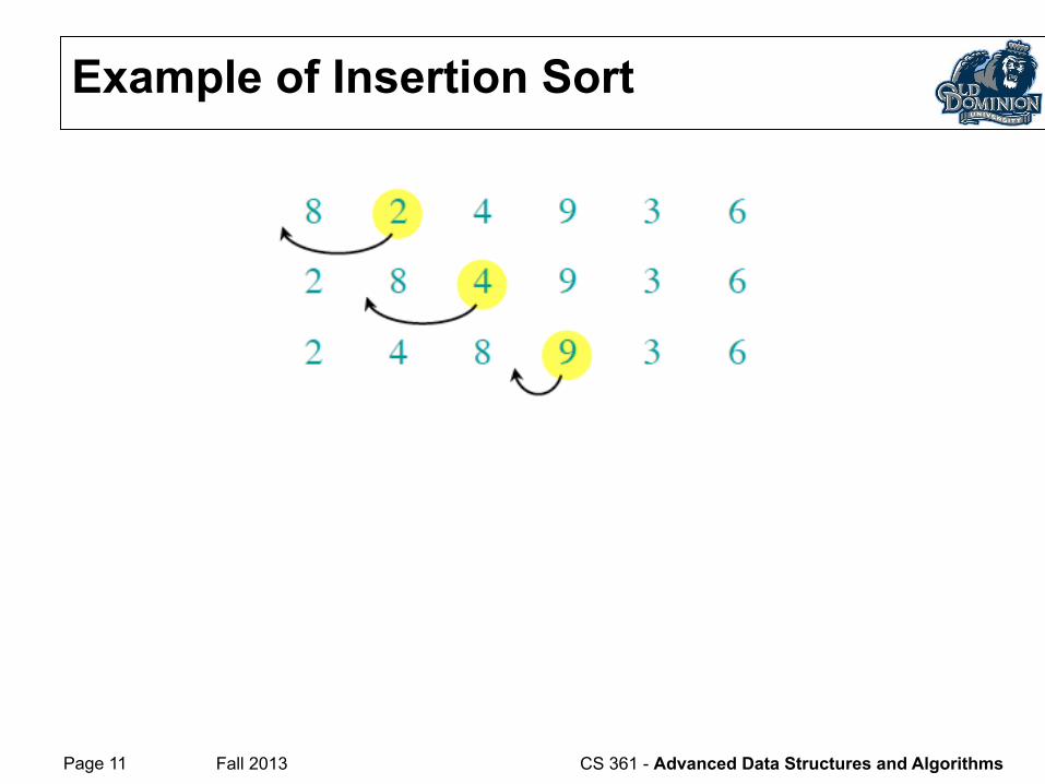
Example of Insertion Sort
Page 12 Fall 2013 CS 361 - Advanced Data Structures and Algorithms
Example of Insertion Sort
Page 13 Fall 2013 CS 361 - Advanced Data Structures and Algorithms
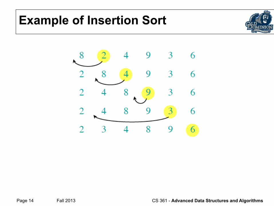
Example of Insertion Sort
Page 14 Fall 2013 CS 361 - Advanced Data Structures and Algorithms
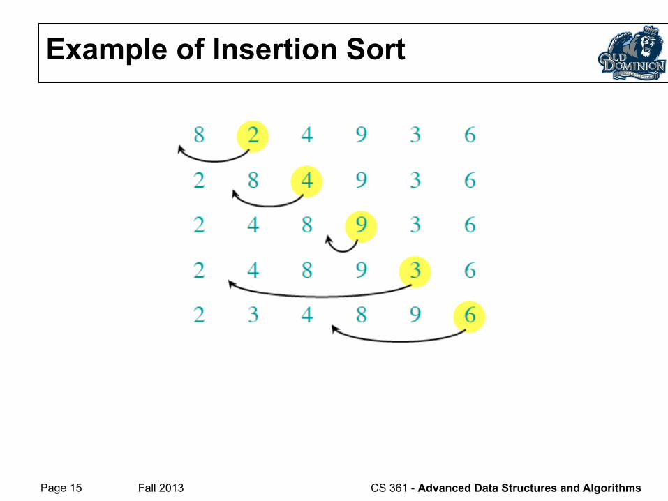
Example of Insertion Sort
Page 15 Fall 2013 CS 361 - Advanced Data Structures and Algorithms
Example of Insertion Sort
Page 16 Fall 2013 CS 361 - Advanced Data Structures and Algorithms
Example of Insertion Sort
Page 17 Fall 2013 CS 361 - Advanced Data Structures and Algorithms
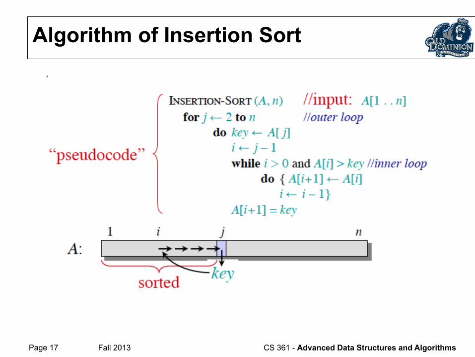
Algorithm of Insertion Sort
Page 18 Fall 2013 CS 361 - Advanced Data Structures and Algorithms
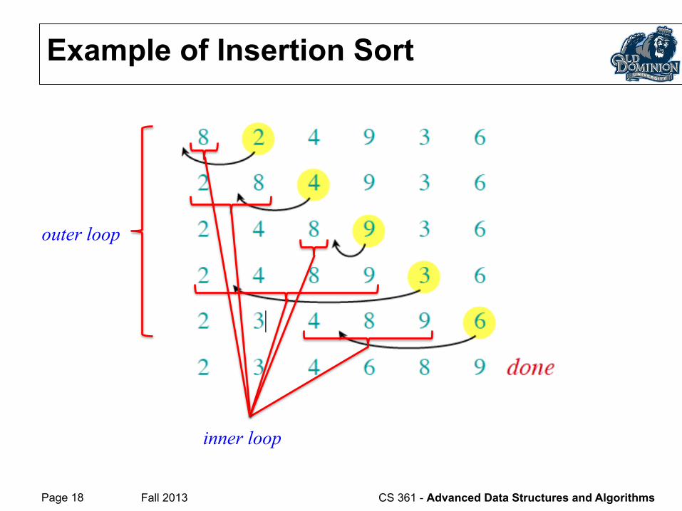
Example of Insertion Sort
outer loop
inner loop
Page 19 Fall 2013 CS 361 - Advanced Data Structures and Algorithms
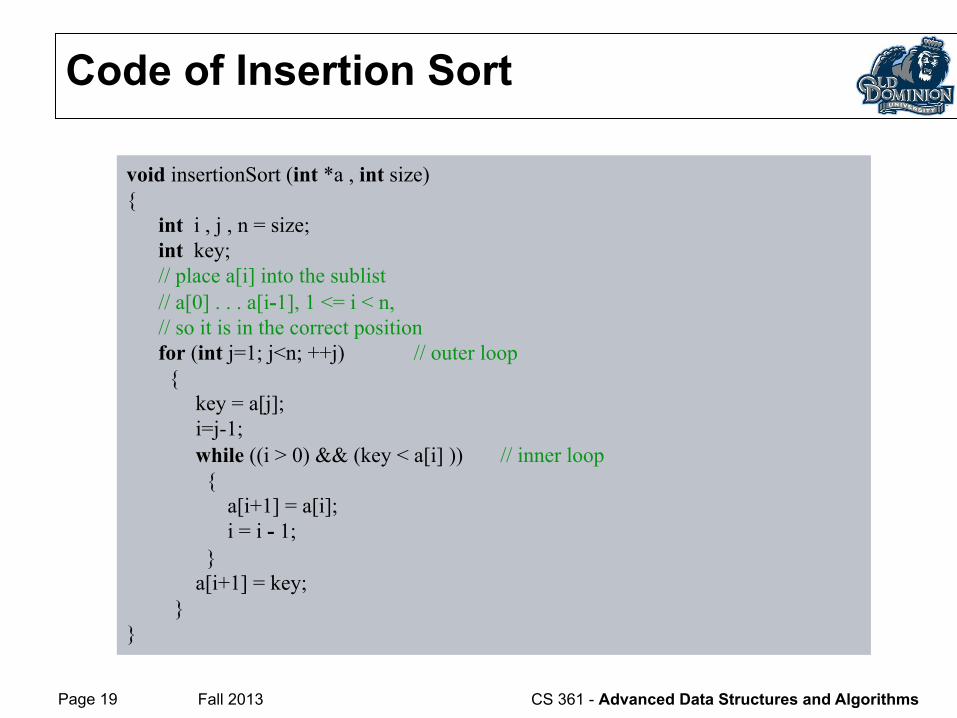
Code of Insertion Sort
void insertionSort (int *a , int size) { int i , j , n = size; int key; // place a[i] into the sublist // a[0] . . . a[i-1], 1 <= i < n, // so it is in the correct position for (int j=1; j<n; ++j) // outer loop { key = a[j]; i=j-1; while ((i > 0) && (key < a[i] )) // inner loop { a[i+1] = a[i]; i = i - 1; } a[i+1] = key; } }
Page 20 Fall 2013 CS 361 - Advanced Data Structures and Algorithms
Comments on Insertion Sort
• If the key value is greater than all the sorted elements in the sublist, the algorithm does 0 iterations of the inner loop.
• If the initial array is sorted: • Then each new key will be greater than all the ones already
inserted into the array. • For each outer loop iteration, the algorithm does 0 iterations of
the inner loop.
• This special case is very common. Many practical problems require the construction of a sorted sequence of elements from a set of data that is already sorted or nearly so, with only a few items out of place.
• Note the "work from the back” is very efficient for such inputs.
Page 21 Fall 2013 CS 361 - Advanced Data Structures and Algorithms
Analysis of Algorithms
Page 22 Fall 2013 CS 361 - Advanced Data Structures and Algorithms
Algorithm Complexity
• A code of an algorithm is judged by its correctness, its ease of use, and its efficiency.
• This course focus on the computational complexity (time efficiency) of algorithms that apply to container objects (data structures) that hold a large collection of data.
• We will learn how to develop measures of efficiency (criteria) that depends on n, the number of data items in the container.
• The criteria of computational complexity often include the number of comparison tests and the number of assignment statements used by the algorithm.
Page 23 Fall 2013 CS 361 - Advanced Data Structures and Algorithms
Running Time
• The term running time is often used to refer to the computational complexity (how fast the algorithm).
• The running time depends on the input (e.g., an already sorted sequence is easier to sort). • Parameterize the running time by the size of the input n • Seek upper bounds on the running time T(n) for the input
size n, because everybody likes a guarantee. • T(n) function counts the frequency of the key operations in
terms of n.
Page 24 Fall 2013 CS 361 - Advanced Data Structures and Algorithms
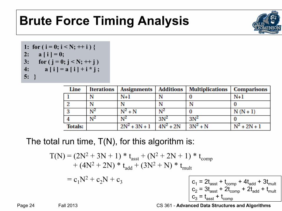
Brute Force Timing Analysis
The total run time, T(N), for this algorithm is: T(N) = (2N2 + 3N + 1) * tasst + (N2 + 2N + 1) * tcomp + (4N2 + 2N) * tadd + (3N2 + N) * tmult
= c1N2 + c2N + c3
1: for ( i = 0; i < N; ++ i ) { 2: a [ i ] = 0; 3: for ( j = 0; j < N; ++ j ) 4: a [ i ] = a [ i ] + i * j ; 5: }
c1 = 2tasst + tcomp + 4tadd + 3tmult c2 = 3tasst + 2tcomp + 2tadd + tmult c3 = tasst + tcomp
Page 25 Fall 2013 CS 361 - Advanced Data Structures and Algorithms
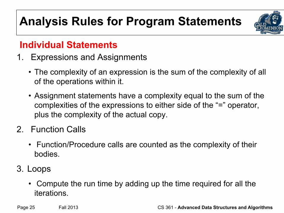
1. Expressions and Assignments
• The complexity of an expression is the sum of the complexity of all of the operations within it.
• Assignment statements have a complexity equal to the sum of the complexities of the expressions to either side of the “=” operator, plus the complexity of the actual copy.
2. Function Calls
• Function/Procedure calls are counted as the complexity of their bodies.
3. Loops
• Compute the run time by adding up the time required for all the iterations.
Analysis Rules for Program Statements
Individual Statements
Page 26 Fall 2013 CS 361 - Advanced Data Structures and Algorithms
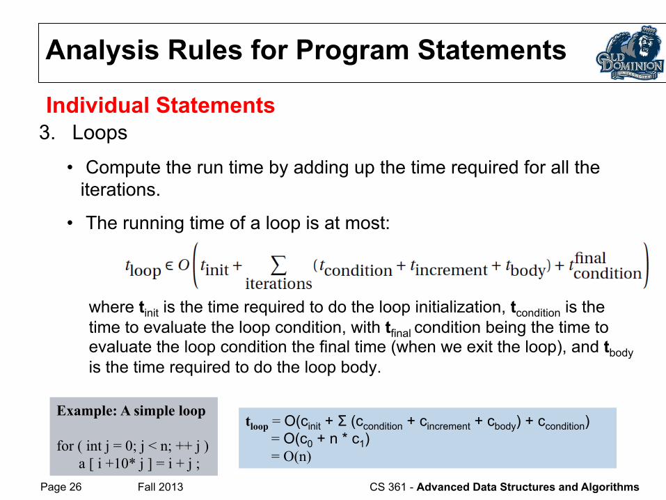
3. Loops
• Compute the run time by adding up the time required for all the iterations.
• The running time of a loop is at most:
where tinit is the time required to do the loop initialization, tcondition is the time to evaluate the loop condition, with tfinal condition being the time to evaluate the loop condition the final time (when we exit the loop), and tbody is the time required to do the loop body.
Analysis Rules for Program Statements
Example: A simple loop for ( int j = 0; j < n; ++ j ) a [ i +10* j ] = i + j ;
tloop = O(cinit + Σ (ccondition + cincrement + cbody) + ccondition) = O(c0 + n * c1) = O(n)
Individual Statements
Page 27 Fall 2013 CS 361 - Advanced Data Structures and Algorithms
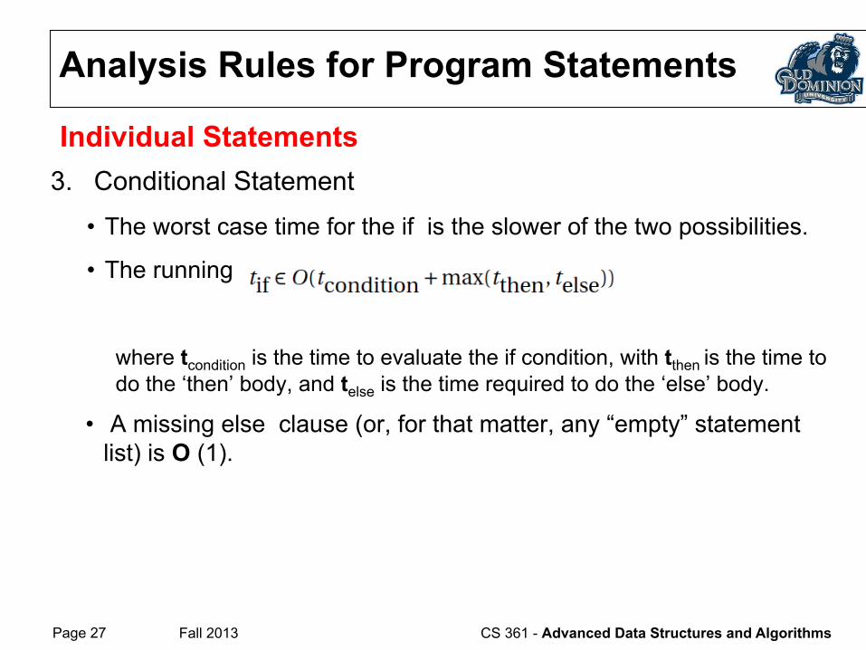
3. Conditional Statement
• The worst case time for the if is the slower of the two possibilities.
• The running time of an if-then-else is at most:
where tcondition is the time to evaluate the if condition, with tthen is the time to do the ‘then’ body, and telse is the time required to do the ‘else’ body.
• A missing else clause (or, for that matter, any “empty” statement list) is O (1).
Analysis Rules for Program Statements
Individual Statements
Page 28 Fall 2013 CS 361 - Advanced Data Structures and Algorithms
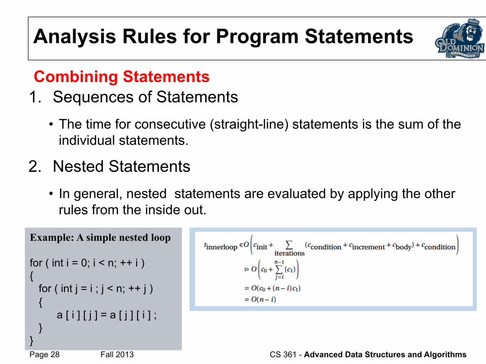
1. Sequences of Statements
• The time for consecutive (straight-line) statements is the sum of the individual statements.
2. Nested Statements
• In general, nested statements are evaluated by applying the other rules from the inside out.
Analysis Rules for Program Statements
Example: A simple nested loop for ( int i = 0; i < n; ++ i ) { for ( int j = i ; j < n; ++ j ) { a [ i ] [ j ] = a [ j ] [ i ] ; } }
Combining Statements
Page 29 Fall 2013 CS 361 - Advanced Data Structures and Algorithms
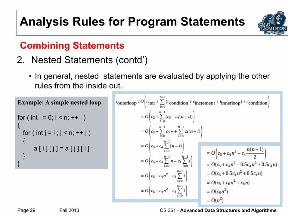
2. Nested Statements (contd’) • In general, nested statements are evaluated by applying the other
rules from the inside out.
Analysis Rules for Program Statements
Example: A simple nested loop for ( int i = 0; i < n; ++ i ) { for ( int j = i ; j < n; ++ j ) { a [ i ] [ j ] = a [ j ] [ i ] ; } }
Combining Statements
Page 30 Fall 2013 CS 361 - Advanced Data Structures and Algorithms
• What is insertion sort’s worst-case time?
• It depends on the speed of our computer:
• relative speed (on the same machine),
• absolute speed (on different machines).
• BIG IDEA:
• Ignore machine-dependent constants.
• Look at growth of T(n) as n à ∞
Machine-independent time
“Asymptotic Analysis”
Page 31 Fall 2013 CS 361 - Advanced Data Structures and Algorithms
Worst Case Analysis
Definition: We say that an algorithm requires time proportional to f(n) if there are constants c and n0 such that the algorithm requires no more than c * f(n) time units to process an input set of size n whenever n ≥ n0.
• The f(n) here describes the rate at which the time required by this algorithm goes up as you change the size of the input for particular program or algorithm.
• The multiplier c is used so that we can talk about the algorithm requiring no more than “c*f(n) time units”.
• n0 is used to place a lower limit on how small the inputs are we really worried about.
Page 32 Fall 2013 CS 361 - Advanced Data Structures and Algorithms
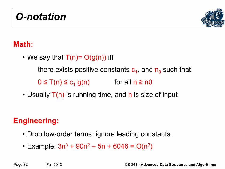
Math: • We say that T(n)= O(g(n)) iff
there exists positive constants c1, and n0 such that
0 ≤ T(n) ≤ c1 g(n) for all n ≥ n0
• Usually T(n) is running time, and n is size of input
Engineering:
• Drop low-order terms; ignore leading constants.
• Example: 3n3 + 90n2 – 5n + 6046 = O(n3)
O-notation
Page 33 Fall 2013 CS 361 - Advanced Data Structures and Algorithms
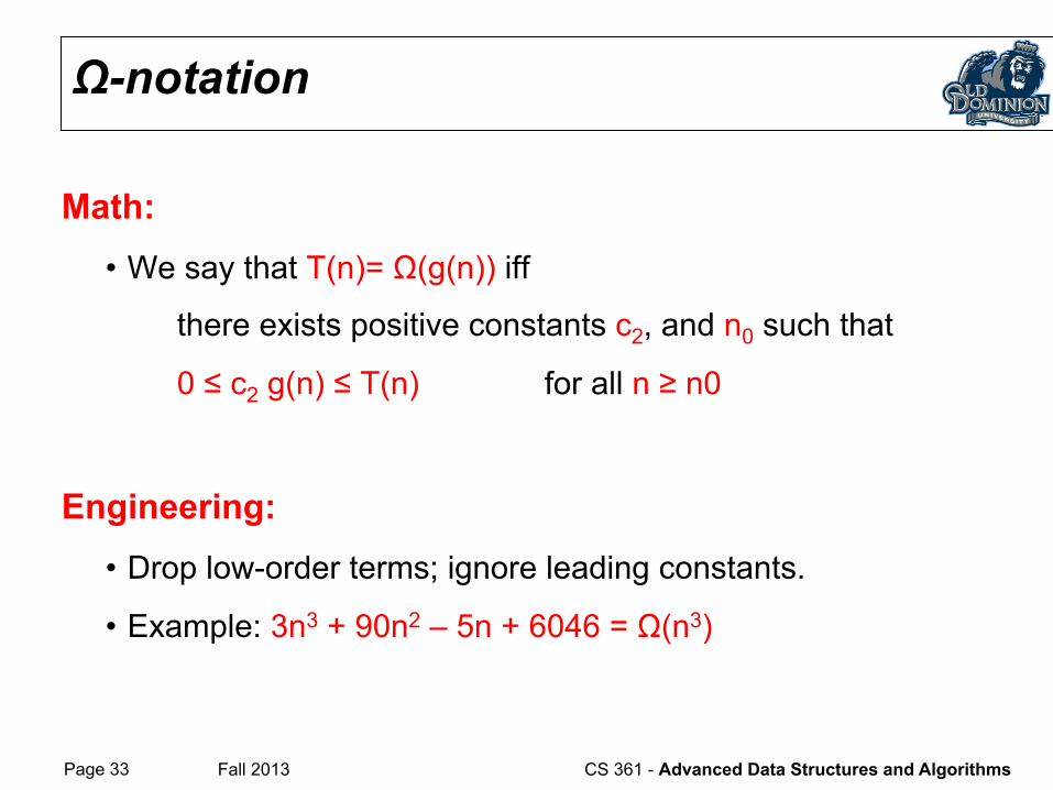
Math: • We say that T(n)= Ω(g(n)) iff
there exists positive constants c2, and n0 such that
0 ≤ c2 g(n) ≤ T(n) for all n ≥ n0
Engineering: • Drop low-order terms; ignore leading constants.
• Example: 3n3 + 90n2 – 5n + 6046 = Ω(n3)
Ω-notation
Page 34 Fall 2013 CS 361 - Advanced Data Structures and Algorithms
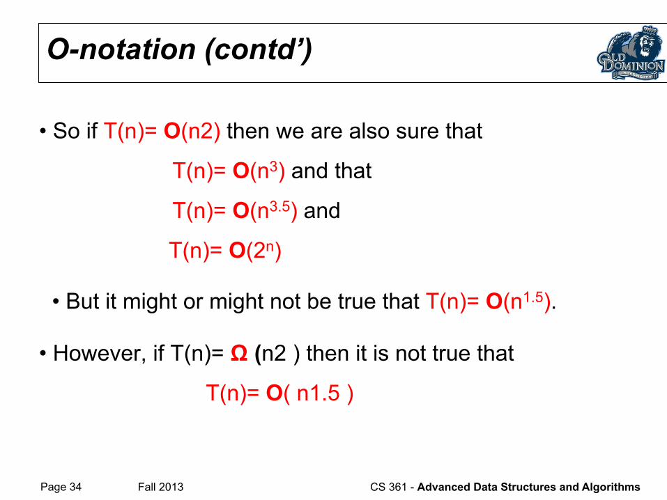
• So if T(n)= O(n2) then we are also sure that
T(n)= O(n3) and that
T(n)= O(n3.5) and
T(n)= O(2n)
• But it might or might not be true that T(n)= O(n1.5).
• However, if T(n)= Ω (n2 ) then it is not true that
T(n)= O( n1.5 )
O-notation (contd’)
Page 35 Fall 2013 CS 361 - Advanced Data Structures and Algorithms
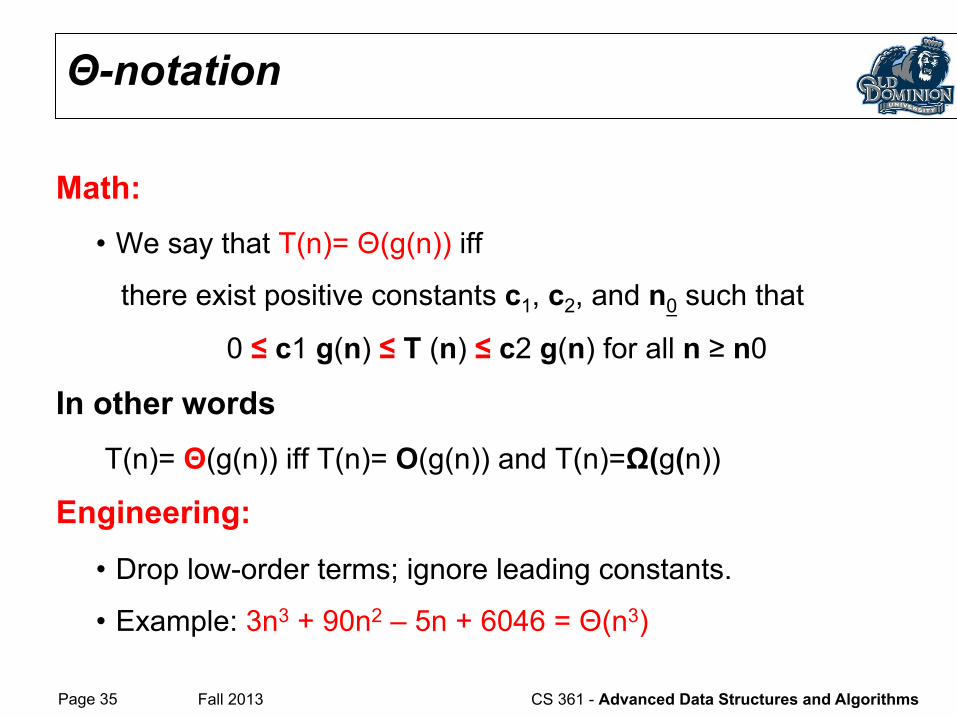
Math: • We say that T(n)= Θ(g(n)) iff
there exist positive constants c1, c2, and n0 such that
0 ≤ c1 g(n) ≤ T (n) ≤ c2 g(n) for all n ≥ n0
In other words T(n)= Θ(g(n)) iff T(n)= O(g(n)) and T(n)=Ω(g(n))
Engineering:
• Drop low-order terms; ignore leading constants.
• Example: 3n3 + 90n2 – 5n + 6046 = Θ(n3)
Θ-notation
Page 36 Fall 2013 CS 361 - Advanced Data Structures and Algorithms
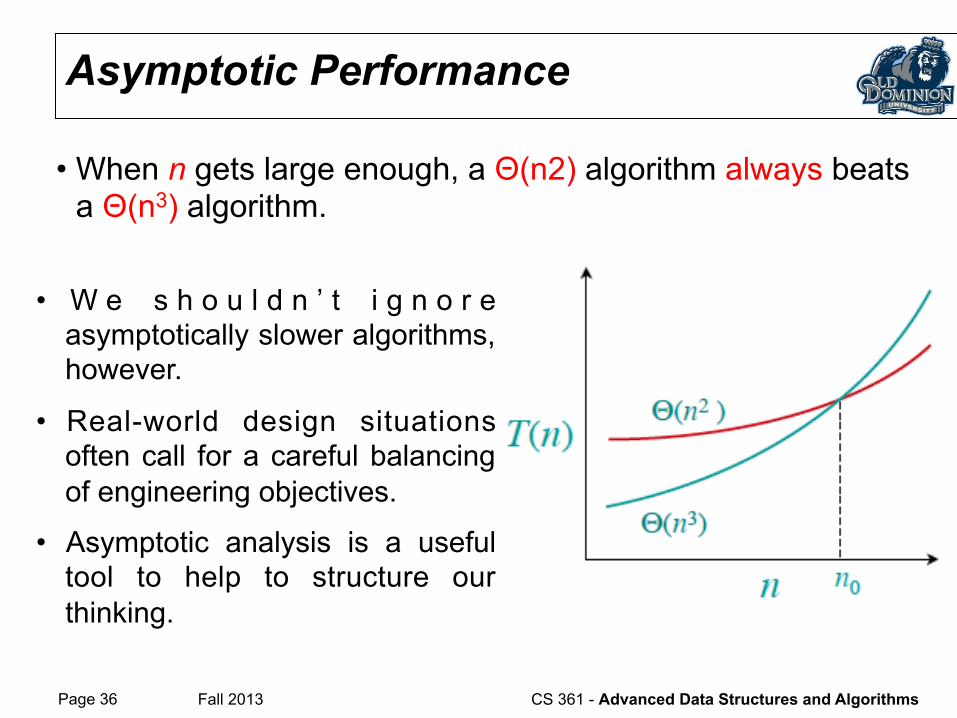
• When n gets large enough, a Θ(n2) algorithm always beats a Θ(n3) algorithm.
Asymptotic Performance
• W e s h o u l d n ’ t i g n o r e asymptotically slower algorithms, however.
• Real-world design situations often call for a careful balancing of engineering objectives.
• Asymptotic analysis is a useful tool to help to structure our thinking.
Page 37 Fall 2013 CS 361 - Advanced Data Structures and Algorithms
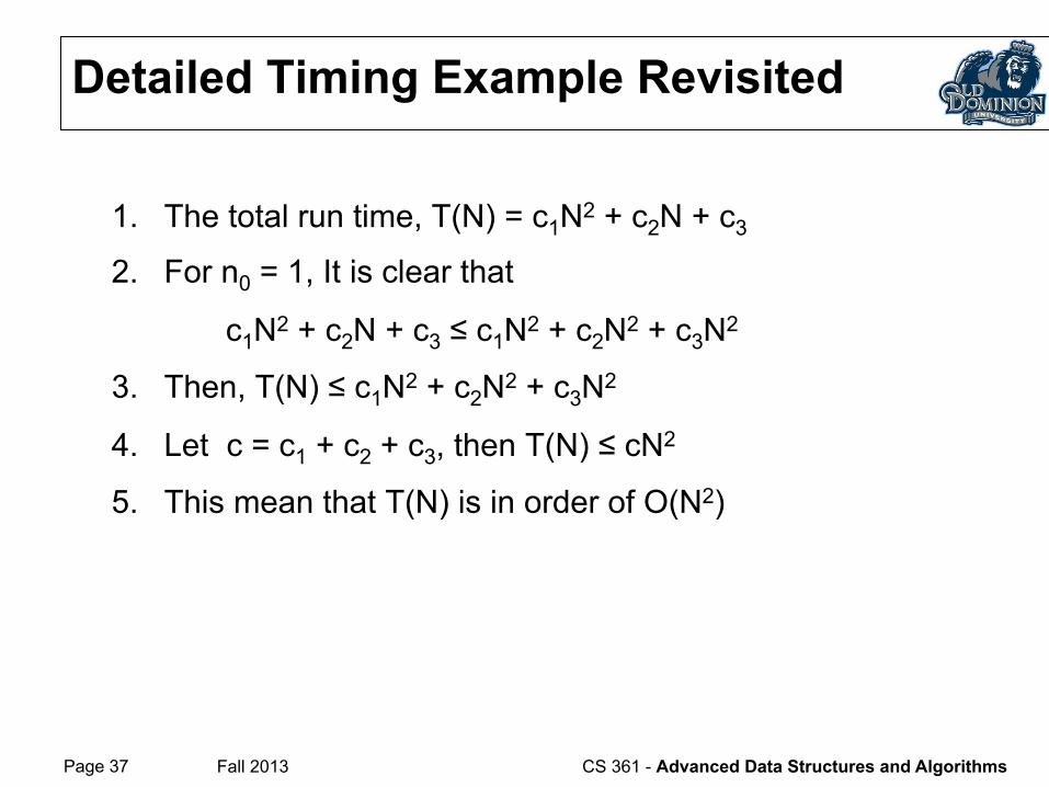
Detailed Timing Example Revisited
1. The total run time, T(N) = c1N2 + c2N + c3
2. For n0 = 1, It is clear that
c1N2 + c2N + c3 ≤ c1N2 + c2N2 + c3N2
3. Then, T(N) ≤ c1N2 + c2N2 + c3N2
4. Let c = c1 + c2 + c3, then T(N) ≤ cN2
5. This mean that T(N) is in order of O(N2)
Page 38 Fall 2013 CS 361 - Advanced Data Structures and Algorithms
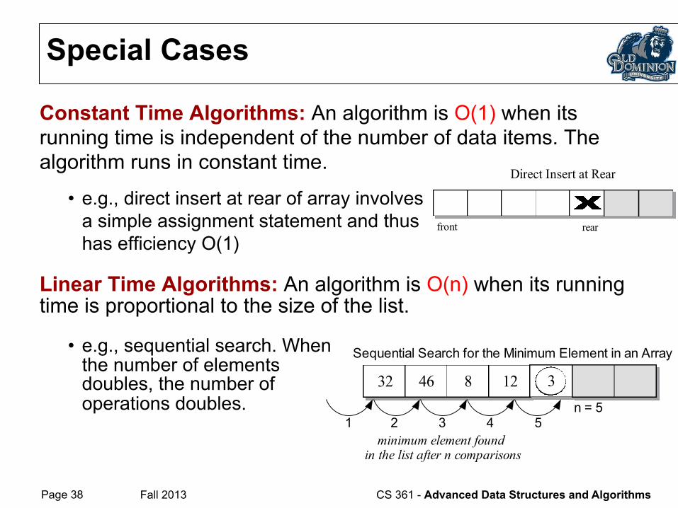
Constant Time Algorithms: An algorithm is O(1) when its running time is independent of the number of data items. The algorithm runs in constant time.
• e.g., direct insert at rear of array involves a simple assignment statement and thus has efficiency O(1)
Linear Time Algorithms: An algorithm is O(n) when its running time is proportional to the size of the list.
• e.g., sequential search. When the number of elements doubles, the number of operations doubles.
Special Cases
front rear
Direct Insert at Rear
Sequential Search for the Minimum Element in an Array
32 46 8 12 3
minimum element found in the list after n comparisons
n = 51 2 3 4 5

Page 39 Fall 2013 CS 361 - Advanced Data Structures and Algorithms
nn2
log2n
Exponential Algorithms: • Algorithms with running time O(n2) are quadratic.
• practical only for relatively small values of n. • Whenever n doubles, the running time of the algorithm increases by
a factor of 4. • Algorithms with running time O(n3) are cubic.
• efficiency is generally poor; doubling the size of n increases the running time eight-fold.
Logarithmic Time Algorithms: The logarithm of n, base 2, is commonly used when analyzing computer algorithms
• Ex. log2(2) = 1, log2(75) = 6.2288 • When compared to the functions
n and n2, the function log2 n grows very slowly
Special Cases
Page 40 Fall 2013 CS 361 - Advanced Data Structures and Algorithms
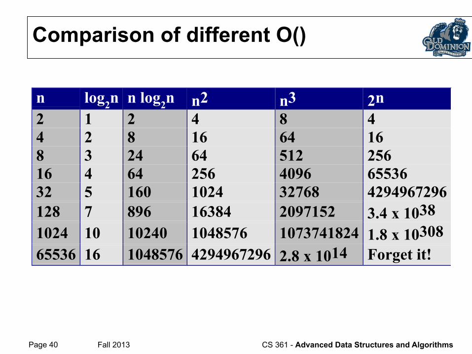
Comparison of different O()
n log2n n log2n n2 n3 2n 2 1 2 4 8 4 4 2 8 16 64 16 8 3 24 64 512 256 16 4 64 256 4096 65536 32 5 160 1024 32768 4294967296 128 7 896 16384 2097152 3.4 x 1038 1024 10 10240 1048576 1073741824 1.8 x 10308 65536 16 1048576 4294967296 2.8 x 10¹⁴ Forget it!
Page 41 Fall 2013 CS 361 - Advanced Data Structures and Algorithms
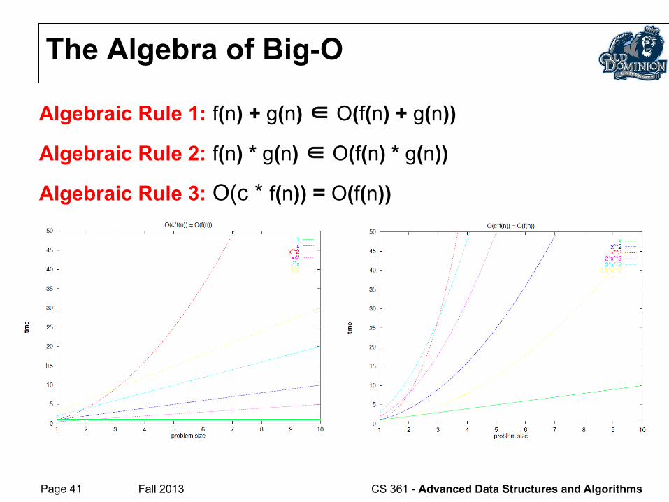
Algebraic Rule 1: f(n) + g(n) ∈ O(f(n) + g(n))
Algebraic Rule 2: f(n) * g(n) ∈ O(f(n) * g(n))
Algebraic Rule 3: O(c * f(n)) = O(f(n))
The Algebra of Big-O
Page 42 Fall 2013 CS 361 - Advanced Data Structures and Algorithms
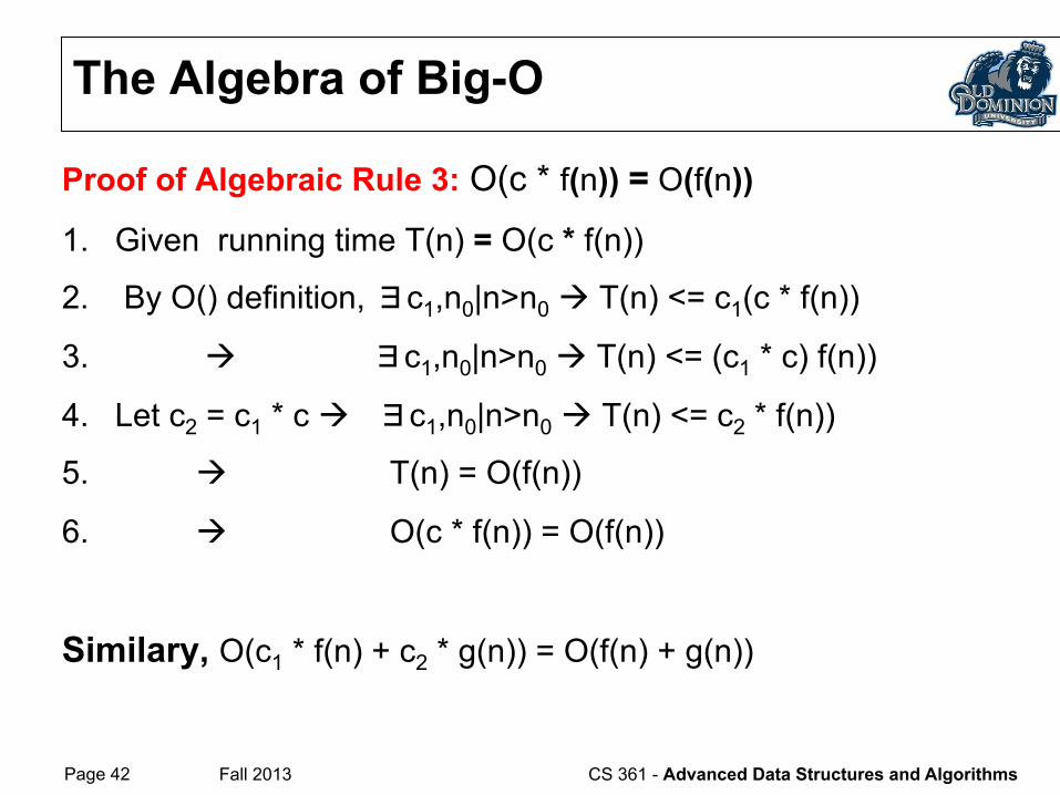
Proof of Algebraic Rule 3: O(c * f(n)) = O(f(n))
1. Given running time T(n) = O(c * f(n))
2. By O() definition, ∃c1,n0|n>n0 à T(n) <= c1(c * f(n))
3. à ∃c1,n0|n>n0 à T(n) <= (c1 * c) f(n))
4. Let c2 = c1 * c à ∃c1,n0|n>n0 à T(n) <= c2 * f(n))
5. à T(n) = O(f(n))
6. à O(c * f(n)) = O(f(n))
Similary, O(c1 * f(n) + c2 * g(n)) = O(f(n) + g(n))
The Algebra of Big-O
Page 43 Fall 2013 CS 361 - Advanced Data Structures and Algorithms
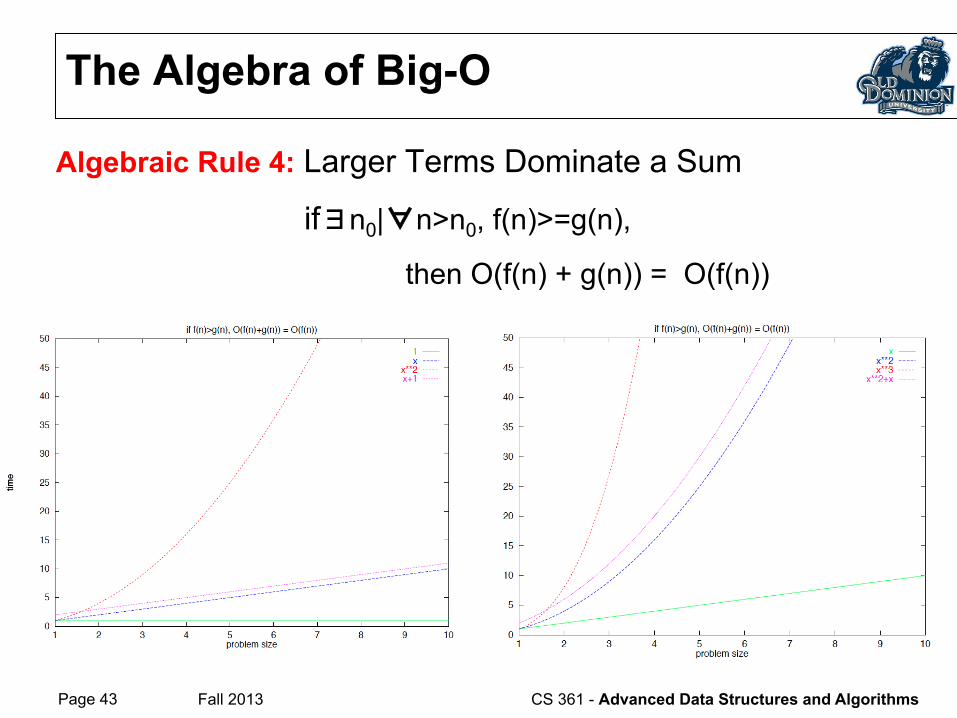
Algebraic Rule 4: Larger Terms Dominate a Sum
if∃n0|∀n>n0, f(n)>=g(n),
then O(f(n) + g(n)) = O(f(n))
The Algebra of Big-O
Page 44 Fall 2013 CS 361 - Advanced Data Structures and Algorithms
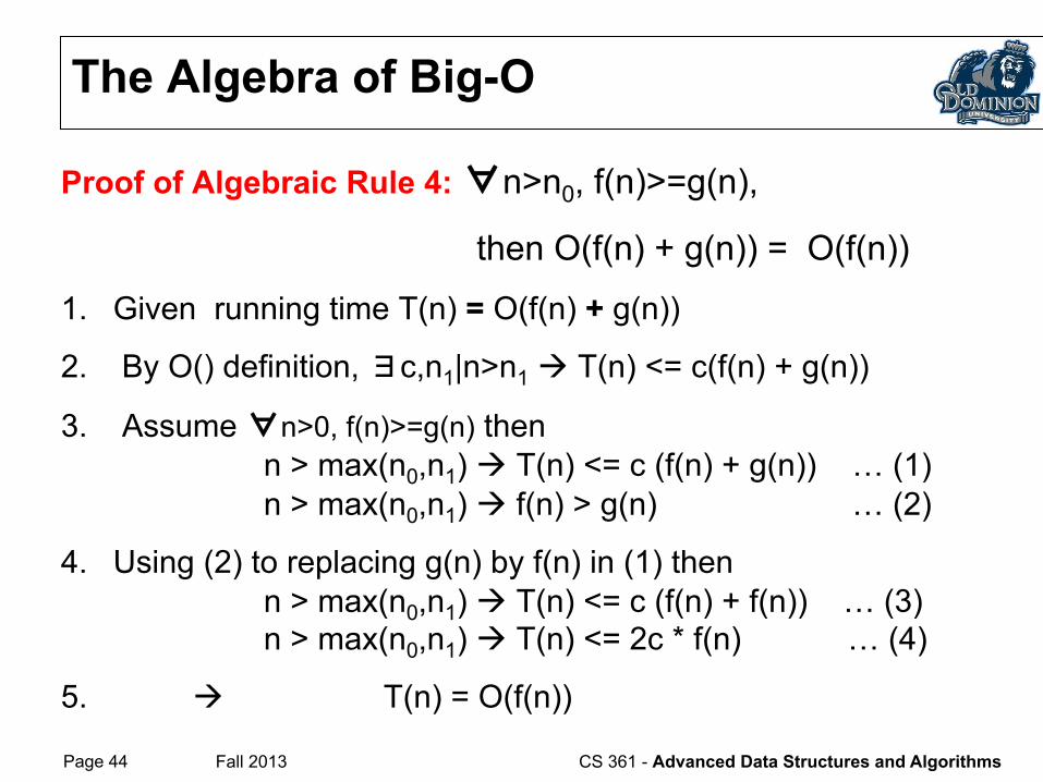
Proof of Algebraic Rule 4: ∀n>n0, f(n)>=g(n),
then O(f(n) + g(n)) = O(f(n))
1. Given running time T(n) = O(f(n) + g(n))
2. By O() definition, ∃c,n1|n>n1 à T(n) <= c(f(n) + g(n))
3. Assume ∀n>0, f(n)>=g(n) then n > max(n0,n1) à T(n) <= c (f(n) + g(n)) … (1) n > max(n0,n1) à f(n) > g(n) … (2)
4. Using (2) to replacing g(n) by f(n) in (1) then n > max(n0,n1) à T(n) <= c (f(n) + f(n)) … (3) n > max(n0,n1) à T(n) <= 2c * f(n) … (4)
5. à T(n) = O(f(n))
The Algebra of Big-O
Page 45 Fall 2013 CS 361 - Advanced Data Structures and Algorithms
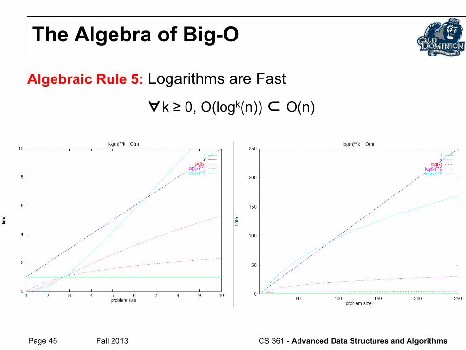
Algebraic Rule 5: Logarithms are Fast
∀k ≥ 0, O(logk(n)) ⊂ O(n)
The Algebra of Big-O
Page 46 Fall 2013 CS 361 - Advanced Data Structures and Algorithms
Analysis of Sorting/Searching
Algorithms

Page 47 Fall 2013 CS 361 - Advanced Data Structures and Algorithms
Algorithm of Insertion Sort
Page 48 Fall 2013 CS 361 - Advanced Data Structures and Algorithms
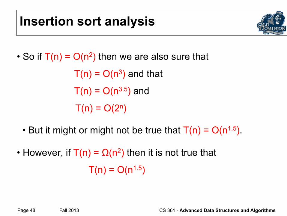
• So if T(n) = O(n2) then we are also sure that
T(n) = O(n3) and that
T(n) = O(n3.5) and
T(n) = O(2n)
• But it might or might not be true that T(n) = O(n1.5).
• However, if T(n) = Ω(n2) then it is not true that
T(n) = O(n1.5)
Insertion sort analysis
Page 49 Fall 2013 CS 361 - Advanced Data Structures and Algorithms
Sequential Search
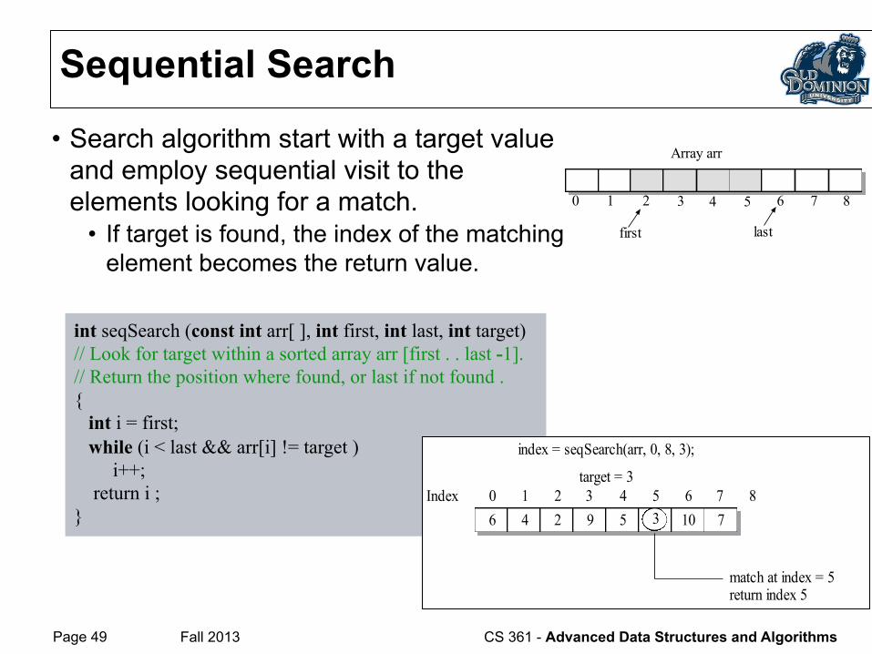
int seqSearch (const int arr[ ], int first, int last, int target) // Look for target within a sorted array arr [first . . last -1]. // Return the position where found, or last if not found . { int i = first; while (i < last && arr[i] != target ) i++; return i ; } 6 4 2 9 5 10
index = seqSearch(arr, 0, 8, 3);
7Index 0 1 2 3 4 5 6 7
3
target = 38
match at index = 5return index 5
• Search algorithm start with a target value and employ sequential visit to the elements looking for a match.
• If target is found, the index of the matching element becomes the return value.
0 1 2 6 7 8
first last
Array arr
543
Page 50 Fall 2013 CS 361 - Advanced Data Structures and Algorithms
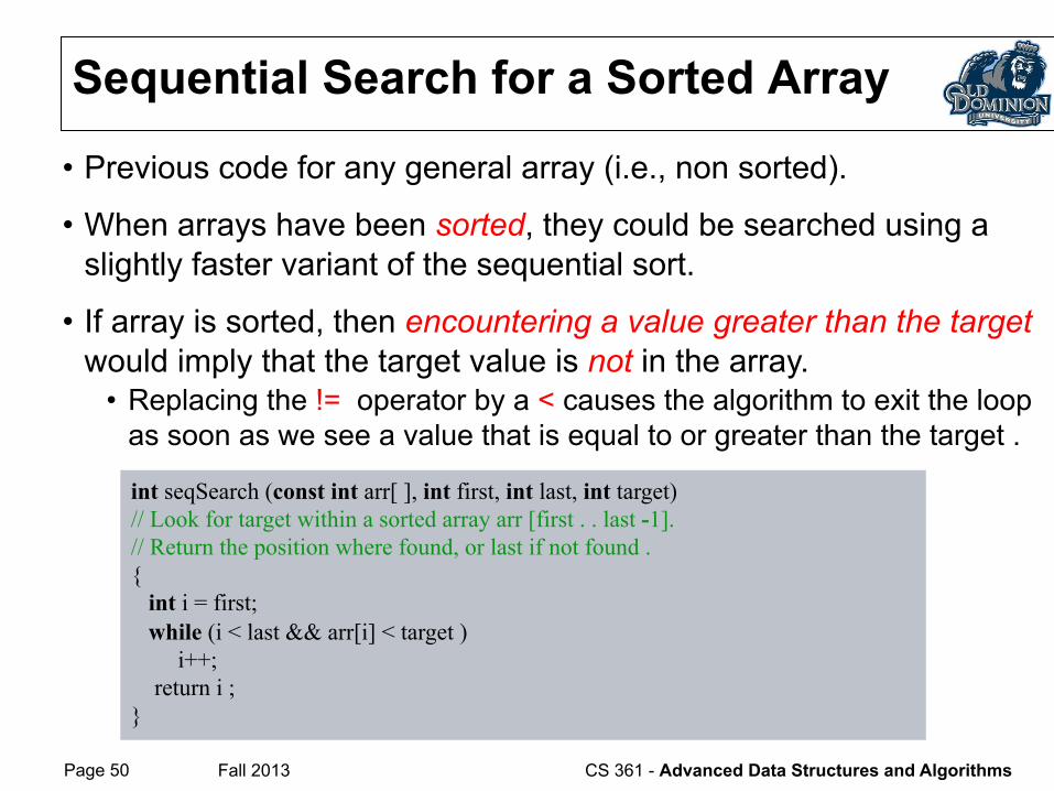
Sequential Search for a Sorted Array
int seqSearch (const int arr[ ], int first, int last, int target) // Look for target within a sorted array arr [first . . last -1]. // Return the position where found, or last if not found . { int i = first; while (i < last && arr[i] < target ) i++; return i ; }
• Previous code for any general array (i.e., non sorted).
• When arrays have been sorted, they could be searched using a slightly faster variant of the sequential sort.
• If array is sorted, then encountering a value greater than the target would imply that the target value is not in the array.
• Replacing the != operator by a < causes the algorithm to exit the loop as soon as we see a value that is equal to or greater than the target .
Page 51 Fall 2013 CS 361 - Advanced Data Structures and Algorithms
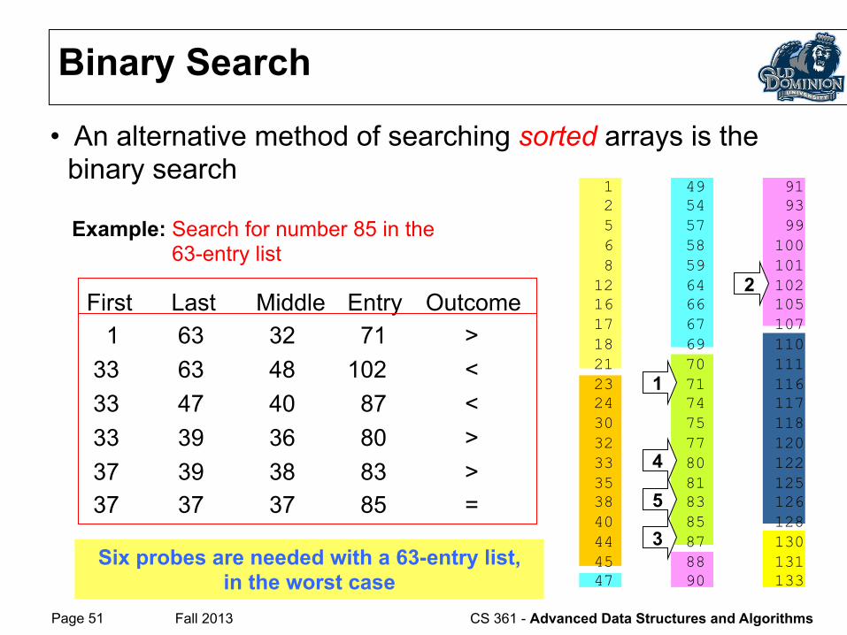
Binary Search
• An alternative method of searching sorted arrays is the binary search
Example: Search for number 85 in the 63-entry list
Six probes are needed with a 63-entry list, in the worst case
1 2 5 6 8
12 16 17 18 21 23 24 30 32 33 35 38 40 44 45 47
49 54 57 58 59 64 66 67 69 70 71 74 75 77 80 81 83 85 87 88 90
91 93 99
100 101 102 105 107 110 111 116 117 118 120 122 125 126 128 130 131 133
1
2
3
4
5
First Last Middle Entry Outcome 1 63 32 71 > 33 63 48 102 < 33 47 40 87 < 33 39 36 80 > 37 39 38 83 > 37 37 37 85 =
Page 52 Fall 2013 CS 361 - Advanced Data Structures and Algorithms
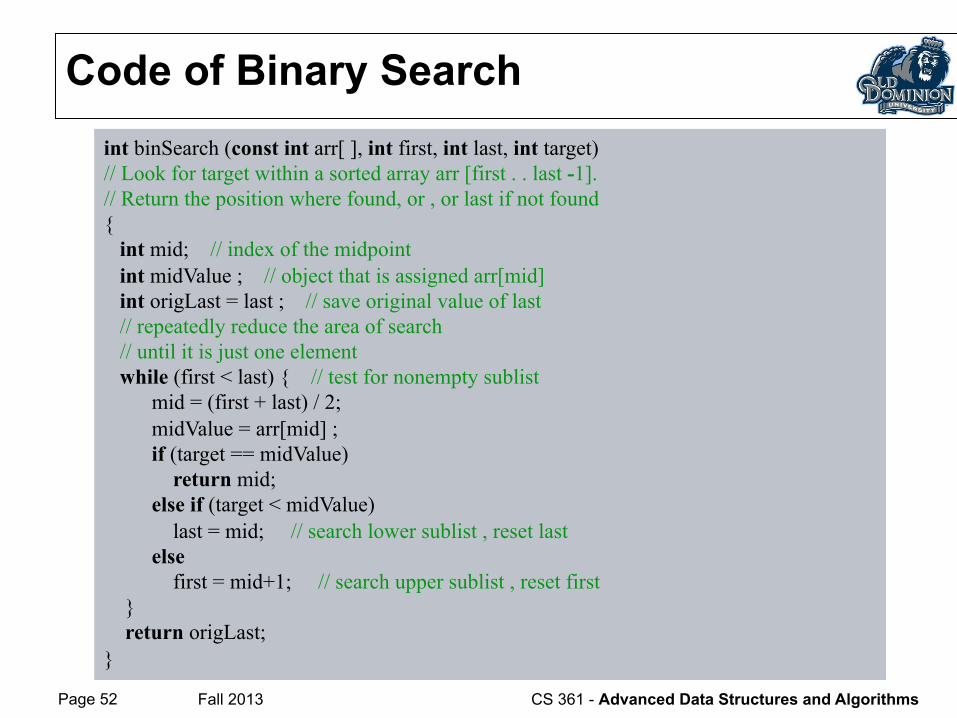
Code of Binary Search int binSearch (const int arr[ ], int first, int last, int target) // Look for target within a sorted array arr [first . . last -1]. // Return the position where found, or , or last if not found { int mid; // index of the midpoint int midValue ; // object that is assigned arr[mid] int origLast = last ; // save original value of last // repeatedly reduce the area of search // until it is just one element while (first < last) { // test for nonempty sublist mid = (first + last) / 2; midValue = arr[mid] ; if (target == midValue) return mid; else if (target < midValue) last = mid; // search lower sublist , reset last else first = mid+1; // search upper sublist , reset first } return origLast; }
Page 53 Fall 2013 CS 361 - Advanced Data Structures and Algorithms
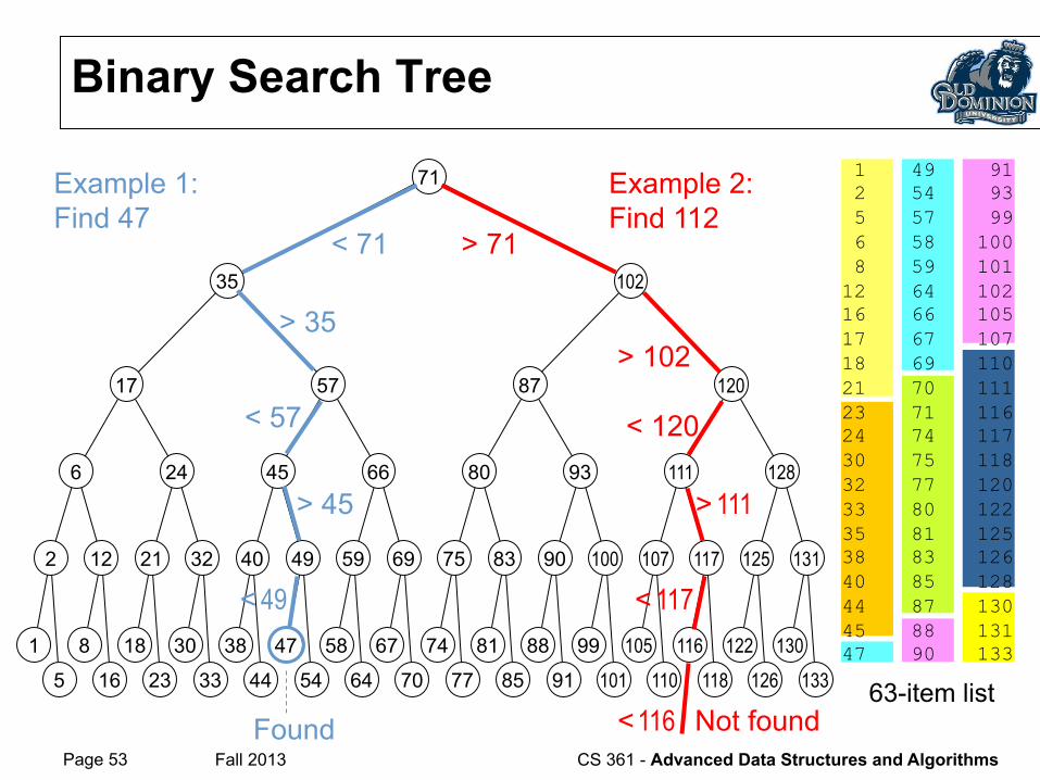
Binary Search Tree
1 2 5 6 8
12 16 17 18 21 23 24 30 32 33 35 38 40 44 45 47
49 54 57 58 59 64 66 67 69 70 71 74 75 77 80 81 83 85 87 88 90
91 93 99
100 101 102 105 107 110 111 116 117 118 120 122 125 126 128 130 131 133 1
5
8
16
18
23
30
33
38
44
47
54
58
64
67
70
74
77
81
85
88
91
99
101 105
110 116
118 122
126 130
133
2 12 21 32 40 49 59 69 75 83 90 100 107 117 125 131
6 24 45 66 80 93 111 128
17 57 87 120
35
71
102
Example 1: Find 47
< 71
> 35
< 57
> 45
< 49
Found 63-item list
Example 2: Find 112
> 71
> 102
< 120
> 111
< 117
< 116 Not found
Page 54 Fall 2013 CS 361 - Advanced Data Structures and Algorithms
Making Algorithms Generic
Page 55 Fall 2013 CS 361 - Advanced Data Structures and Algorithms
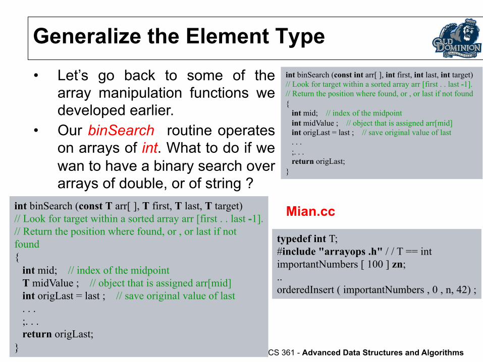
Generalize the Element Type • Let’s go back to some of the
array manipulation functions we developed earlier.
• Our binSearch routine operates on arrays of int. What to do if we wan to have a binary search over arrays of double, or of string ?
int binSearch (const int arr[ ], int first, int last, int target) // Look for target within a sorted array arr [first . . last -1]. // Return the position where found, or , or last if not found { int mid; // index of the midpoint int midValue ; // object that is assigned arr[mid] int origLast = last ; // save original value of last . . . ;. . . return origLast; }
int binSearch (const T arr[ ], T first, T last, T target) // Look for target within a sorted array arr [first . . last -1]. // Return the position where found, or , or last if not found { int mid; // index of the midpoint T midValue ; // object that is assigned arr[mid] int origLast = last ; // save original value of last . . . ;. . . return origLast; }
typedef int T; #include "arrayops .h" / / T == int importantNumbers [ 100 ] zn; .. orderedInsert ( importantNumbers , 0 , n, 42) ;
Mian.cc
Page 56 Fall 2013 CS 361 - Advanced Data Structures and Algorithms
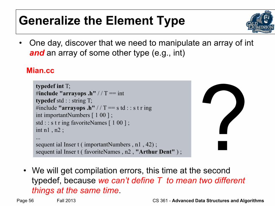
Generalize the Element Type • One day, discover that we need to manipulate an array of int
and an array of some other type (e.g., int)
typedef int T; #include "arrayops .h" / / T == int typedef std : : string T; #include "arrayops .h" / / T == s td : : s t r ing int importantNumbers [ 1 00 ] ; std : : s t r ing favoriteNames [ 1 00 ] ; int n1 , n2 ; ... sequent ial Inser t ( importantNumbers , n1 , 42) ; sequent ial Inser t ( favoriteNames , n2 , "Arthur Dent" ) ;
Mian.cc
? • We will get compilation errors, this time at the second
typedef, because we can’t define T to mean two different things at the same time.
Page 57 Fall 2013 CS 361 - Advanced Data Structures and Algorithms
Generalize the Element Type
• we could simply make a distinct copy of binSearch for each kind of array, using an ordinary text editor to replace T by a “real” type name.
• Doing this in a large program does get to be a bit of a project management headache.
• Since it is a common situation, and it does involve a fair amount of work, some programming language designers (e.g., C++) eventually found a way to do the same thing automatically; use of Templates.
Page 58 Fall 2013 CS 361 - Advanced Data Structures and Algorithms
Templates in C++ • Templates describe common “patterns” for similar classes
and functions that differ only in a few names.
• Templates come in two varieties: Class templates, and Function templates
• Class templates are patterns for similar classes. Function templates are patterns for similar function
• A C++ template is a kind of pattern for code in which certain names that, like T in the earlier example, we intend to replace by something “real” when we use the pattern. These names are called template parameters.
• The compiler instantiates (creates an instance of) a template by filling in the appropriate replacement for these template parameter names, thereby generating the actual code for a function or class, and compiling that instantiated code.
Page 59 Fall 2013 CS 361 - Advanced Data Structures and Algorithms
Writing Function Templates
• We define a template header for each function to tell the compiler which names in the “pattern” are to be replaced.
• The template header indicates that this is a “pattern” for a function in which certain type names and constants are left to be filled in later.
• The header begins with the key word “template”. After that, inside the “< >”, is a list of all type (class) names to be replaced when we instantiate the template.
• Bodies of function templates are defined in header files (.h)
Page 60 Fall 2013 CS 361 - Advanced Data Structures and Algorithms
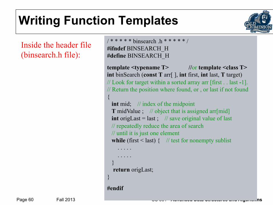
Writing Function Templates / * * * * * binsearch .h * * * * * / #ifndef BINSEARCH_H #define BINSEARCH_H
template <typename T> //or template <class T> int binSearch (const T arr[ ], int first, int last, T target) // Look for target within a sorted array arr [first . . last -1]. // Return the position where found, or , or last if not found { int mid; // index of the midpoint T midValue ; // object that is assigned arr[mid] int origLast = last ; // save original value of last // repeatedly reduce the area of search // until it is just one element while (first < last) { // test for nonempty sublist . . . . . . . . . . } return origLast; }
#endif
Inside the header file (binsearch.h file):
Page 61 Fall 2013 CS 361 - Advanced Data Structures and Algorithms
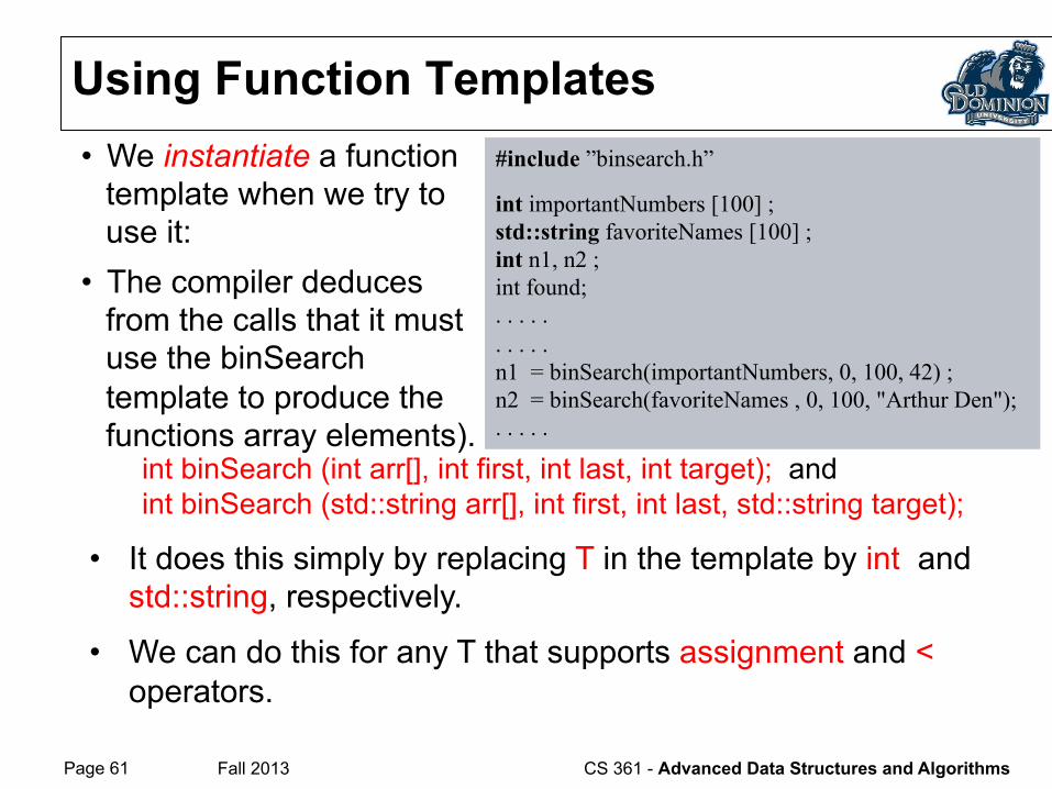
Using Function Templates • We instantiate a function
template when we try to use it:
#include ”binsearch.h”
int importantNumbers [100] ; std::string favoriteNames [100] ; int n1, n2 ; int found; . . . . . . . . . . n1 = binSearch(importantNumbers, 0, 100, 42) ; n2 = binSearch(favoriteNames , 0, 100, "Arthur Den"); . . . . .
• The compiler deduces from the calls that it must use the binSearch template to produce the functions array elements).
int binSearch (int arr[], int first, int last, int target); and int binSearch (std::string arr[], int first, int last, std::string target);
• It does this simply by replacing T in the template by int and std::string, respectively.
• We can do this for any T that supports assignment and < operators.

Page 62 Fall 2013 CS 361 - Advanced Data Structures and Algorithms
Function Templates and the C++ std Library
• The C++ std library has a number of useful templates for small, common programming idioms.
template <typename T> inline void swap(T& a , T& b) { T tmp = a; a = b; b = tmp; }
• swap Function
template <typename T> inline const T& min(const T& a, const T& b) { return b < a ? b : a ; }
template <typename T> inline const T& max(const T& a, const T& b) { return b < a ? a : b; }
• min & max Functions
• relops Function namespace relops {
template <typename T> inline bool operator!= (const T& a, const T& b){ return !(a == b); } template <typename T> inline bool operator> (const T& a, const T& b){ return b < a; } template <typename T> inline bool operator<= (const T& a, const T& b){ return !(b < a); } template <typename T> inline bool operator>= (const T& a, const T& b){ return !(a < b) ; } }
Page 63 Fall 2013 CS 361 - Advanced Data Structures and Algorithms
Recurssion
Page 64 Fall 2013 CS 361 - Advanced Data Structures and Algorithms
The Concept of Recursion
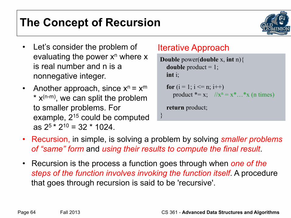
• Let’s consider the problem of evaluating the power xn where x is real number and n is a nonnegative integer.
Double power(double x, int n){
double product = 1; int i;
for (i = 1; i <= n; i++) product *= x; //xn = x*…*x (n times)
return product; }
Iterative Approach
• Another approach, since xn = xm * x(n-m), we can split the problem to smaller problems. For example, 215 could be computed as 25 * 210 = 32 * 1024.
• Recursion, in simple, is solving a problem by solving smaller problems of “same” form and using their results to compute the final result.
• Recursion is the process a function goes through when one of the steps of the function involves invoking the function itself. A procedure that goes through recursion is said to be 'recursive'.
Page 65 Fall 2013 CS 361 - Advanced Data Structures and Algorithms
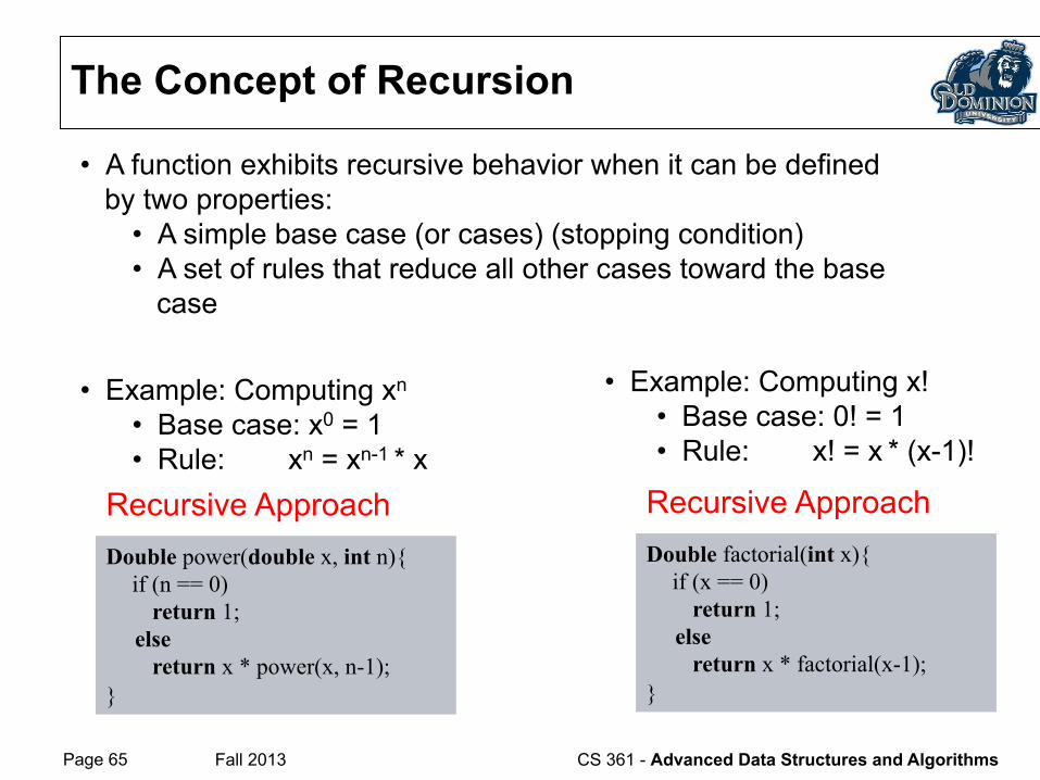
The Concept of Recursion
Double power(double x, int n){
if (n == 0) return 1; else return x * power(x, n-1); }
Recursive Approach
• A function exhibits recursive behavior when it can be defined by two properties:
• A simple base case (or cases) (stopping condition) • A set of rules that reduce all other cases toward the base
case
• Example: Computing xn
• Base case: x0 = 1 • Rule: xn = xn-1 * x
Double factorial(int x){
if (x == 0) return 1; else return x * factorial(x-1); }
Recursive Approach
• Example: Computing x! • Base case: 0! = 1 • Rule: x! = x * (x-1)!

Page 66 Fall 2013 CS 361 - Advanced Data Structures and Algorithms
Fibonacci Numbers
int fib(int n){
if (n <= 1) return n; else return fib(n-1) + fib(n-2); }
Recursive Approach
• Fibonacci numbers are the sequence of integers 0, 1, 1, 2, 3, 5, 8, 13, 21, 34, 55, …
• Example: Computing fib(n) //Fibonacci element with index n
• Base case: fib(0) = 0 fib(1) = 1
• Rule: fib(n) = fib(n-1) + fib(n-2) int fibiter(int n){
int oneback = 1, twoback = 0, current, i;
if (n <= 1) return n; else for (i=2; i <= n; i++){ current = oneback + twoback; twoback = oneback; oneback = current; } return current; }
Iterative Approach
Page 67 Fall 2013 CS 361 - Advanced Data Structures and Algorithms
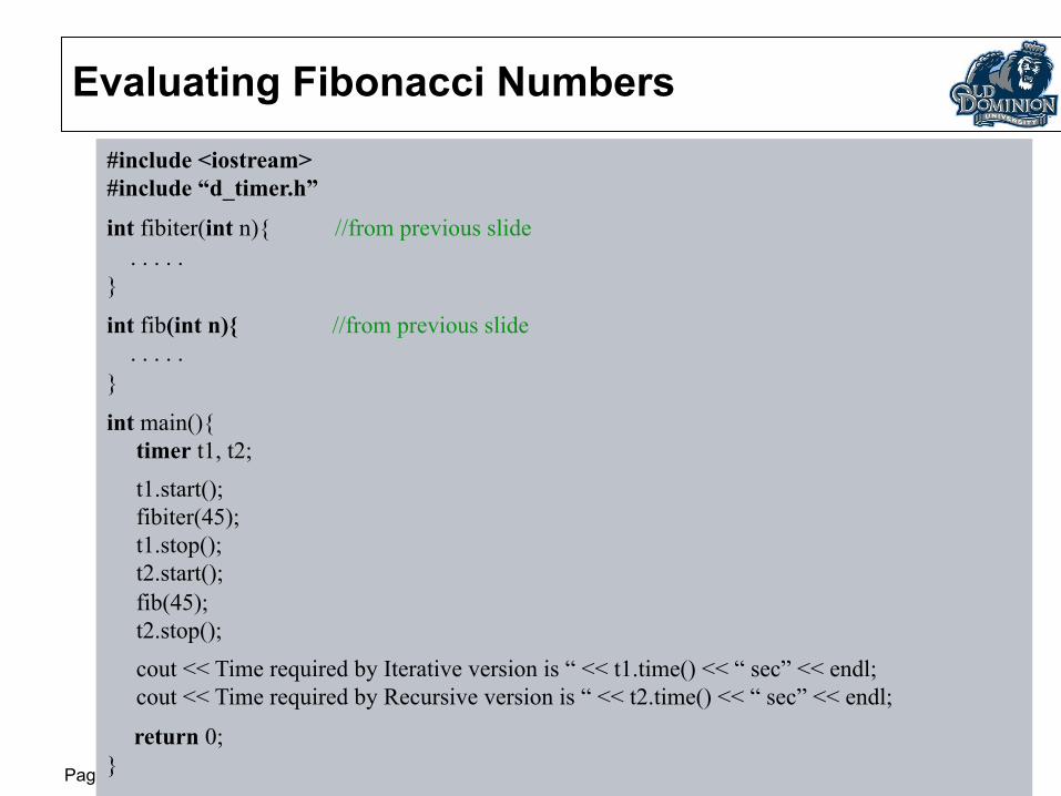
Evaluating Fibonacci Numbers #include <iostream> #include “d_timer.h”
int fibiter(int n){ //from previous slide . . . . . }
int fib(int n){ //from previous slide . . . . . }
int main(){ timer t1, t2;
t1.start(); fibiter(45); t1.stop(); t2.start(); fib(45); t2.stop();
cout << Time required by Iterative version is “ << t1.time() << “ sec” << endl; cout << Time required by Recursive version is “ << t2.time() << “ sec” << endl;
return 0; }

Page 68 Fall 2013 CS 361 - Advanced Data Structures and Algorithms
Tower of Hanoi
Needle A
. . . . . . . .
Needle CNeedle B Needle C
. . . . . . . .
Needle BNeedle A

Page 69 Fall 2013 CS 361 - Advanced Data Structures and Algorithms
Tower of Hanoi
Needle A Needle B Needle C
1
Needle B Needle CNeedle A
2
3
Needle A Needle B Needle C Needle A Needle B Needle C
Needle A Needle B Needle C Needle A Needle B Needle C
4
Needle A Needle B Needle C Needle A Needle B Needle C
56
Needle A Needle B Needle C Needle A Needle B Needle C
7
Page 70 Fall 2013 CS 361 - Advanced Data Structures and Algorithms
Questions?