advanced excel academicacademicacademic for windows · advanced excel for windows...

Advanced ExcelAdvanced ExcelAdvanced ExcelAdvanced Excelfor Windowsfor Windowsfor WindowsVersion: 2002Version: 2002Version: 2002Version: 2002

Advanced Excel for Windowsfor Windows Version: 2002

AcademicAcademicAcademicAcademicComputingComputingComputing

SupportSupportSupport

Academic ComputingComputing

SupportSupport

Information Technology Services Tennessee Technological University

October 2003

1. Opening Excel

In the PC labs, from the Start menu, All Programs Microsoft Office XP Microsoft Excel. Otherwise, under the Start menu, select Programs Microsoft Excel.

2. Creating a Document

Excel opens with a blank spreadsheet. Close this and for this class, open an existing file in the PC lab:

• Select File Open. • From the pulldown menu, select ClassFiles

on ‘Athena’ (F:). • Select the subdirectory

ITS Excel Class Expenses.xls • Click the Open button. • Save the document to My Documents.

You will see a spreadsheet that has been started, but not completed.

See Beginning Excel for details on how a spreadsheet like this is created. Available on the web at http://www.tntech.edu/its/pubs/.

3. Adding Rows for a Title at the Top of the Document

To insert three rows for a title at the top of this document:

• Click on the row header 1 and drag down to row header 3 to highlight rows 1 through 3.

• From the menu, select Insert Rows. • Or right click and select Insert from the popup menu.

Note the existing rows move down the page and three blank rows are inserted above row 1.

Information Technology Services October 2003


Advanced Excel for Windows

3. Adding Rows for a Title at the Top of the Document (cont.)

You can also insert rows or columns by selecting the rows or columns and right-clicking. Select Insert from the floating menu and the rows or columns will be inserted.

Add a title:

• Use Ctrl + Home or your mouse to move to the first cell, A1. • Type: American Travel Expenses • Move to cell A2 and type a single quote mark to indicate that the information you will be

typing should be considered to be text and not as a date. • Type: ‘July 2003

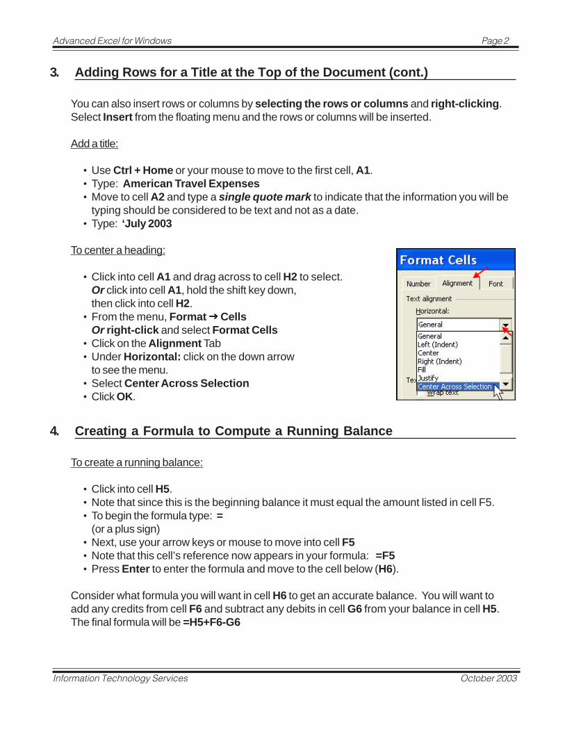
To center a heading:

• Click into cell A1 and drag across to cell H2 to select. Or click into cell A1, hold the shift key down, then click into cell H2.

• From the menu, Format Cells Or right-click and select Format Cells

• Click on the Alignment Tab • Under Horizontal: click on the down arrow

to see the menu. • Select Center Across Selection • Click OK.

4. Creating a Formula to Compute a Running Balance

To create a running balance:

• Click into cell H5. • Note that since this is the beginning balance it must equal the amount listed in cell F5. • To begin the formula type: =

(or a plus sign) • Next, use your arrow keys or mouse to move into cell F5 • Note that this cell’s reference now appears in your formula: =F5 • Press Enter to enter the formula and move to the cell below (H6).

Consider what formula you will want in cell H6 to get an accurate balance. You will want to add any credits from cell F6 and subtract any debits in cell G6 from your balance in cell H5. The final formula will be =H5+F6-G6



4. Creating a Formula to Compute a Running Balance (cont.)

To most easily type this in: • Type: = • Use your arrow keys or mouse to move to cell H5 • Type + • Move to cell F6 • Type - • Move to cell G6 • Press Enter

Note that the same formula will apply down the column with the next row of cells as the references. Excel will automatically adjust your formulas to reflect the change in row position as you copy down the column.

• Click on the cell H6 • Click on the Copy button or from the file menu select Edit Copy

or right-click and select Copy • Click on the cell H7 • Use the scroll bar to move down in the spreadsheet. • Hold the shift key down and click in cell H38 to select the cells from H7 through H38 • Click on the Paste button or from the file menu, select Edit Paste

or right-click and select Paste

Click into several cells from H7 to H38 to see how the formula was adjusted in each row.

5. Computing the Minimum and Maximum Balance

To create a formula for the minimum and maximum balances:

• Click into cell H41 and type: Min Balance: • Click into cell H42 and type: Max Balance:

Expand the width of column H to accommodate this text.

• Move the mouse pointer to the right boundary of the column H header until it changes to a double headed arrow | and drag.

• Or select the column by right-clicking in the header and selecting Column Width • Or from the menu, Format Column Width. Then type a value, such as 12.

Enter the formulas: • Click into cell I41 and type: =min( • Click into cell H5 and drag down through cell H38 • Press Enter and note that the final parenthesis in the formula is completed for you. • Repeat these steps in cell I42 for the maximum value formula which is: =max(h5:h38)



6. Using the If Function to Assign Expenses to Accounting Lines

To categorize your expenses, the If function can be helpful. This function allows you to set a condition for determining what the value of a cell should be. The general form of an If state-ment is: =If(comparison statement, true action, false action)

For example, if the category code in column E is 1, then you would like that amount to be listed in column J under Salary expenses, but if it is not 1, then you would like to show no expense in column E. Consider cell J5: If E5=1, then you would like the value of cell J5 to be equal to the amount in G5, but if the value of E5 is not 1 (Salary), you would want the value of cell J5 to be zero. This can be written as =If(E5=1,G5,0)

Likewise, if the category code in column E is 2, you want the expense to be listed under General expenses in column K and if the category code in column E is 3, then the expense belongs under Supplies in column L. If a deposit has been made, then that amount should be listed under column M (Income).

Enter the formula into cell J5:

• Click into cell J5 • Type: =IF(E5=1,G5,0) • Press Enter and compare your formula with that shown here. Correct any typos.

Tip: You can also enter this formula by clicking in to cell J5, typing =IF( then clicking into cell E5, typing =1 then clicking into G5, typing ,0 and pressing enter.

Repeat the appropriate formula for cells K5 (General), L5 (Supplies), and M5 (Income):

• Click into cell K5 and type: =IF(E5=2,G5,0) • Click into cell L5 and type: =IF(E5=3,G5,0)

To type the comparison in M5, you will need to enclose the category in quotes, because it is text “In” and not a number as in the cases above. Also note that the value comes from cell F5 in this case, not G5 as in the other cells above.

• Click into cell M5 and type: =IF(E5=”In”,F5,0)

Use copy and paste to copy the formulas down each column:

• Select the cells J5 through M5 • Right-click and select Copy • Click on the cell J6 • Use the scroll bar to move down in the spreadsheet. • Hold the shift key down and click in cell M38 to select the cells from J6 through M38 • Right-click and select Paste • Press the Escape key to turn off the selection around the cell you copied from.

• Click into several cells and note how the formulas are copied and adjusted for each row.



7. Using the Sum Function to Total Expenses

To compute the total expenses under each category:

• Click into cell J39 and drag across to select cells K39 and M39.

• Right-click in the highlighted region and select Format Cells from the floating menu or from the menu, select Format Cells

• Select the Border tab • Click on the Top border button to place a plain line

across the top of these cells.

• Click in cell J39. • Click on the AutoSum button. • Note that the formula is correct.

=SUM(J5:J38) • Press Enter. • Copy the formula from cell J39 to cells K39 through M39 using Copy and Paste.

8. Formatting Cells

To format the cells:

• Click in cell J5 • Scroll down the page. • Hold the shift key • Click into cell M39 • Right-click and select Format Cells • Select the Number tab • Under Category:

select Accounting • Under Symbol: select None. • Click OK.

This same formatting is available as a button in the toolbar.

• Click on the Comma Style button

• Try out the other button formatting shortcuts includ-ing $ (accounting currency style), and % (auto-matically converts decimal numbers to percent-ages).

• You may also quickly increase or decrease the number of decimal points displayed by using the Increase Decimal or Decrease Decimal buttons.



9. Plotting the Balances

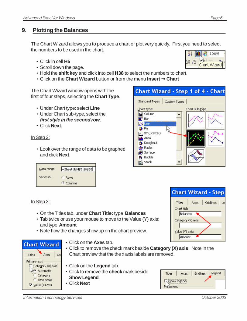
The Chart Wizard allows you to produce a chart or plot very quickly. First you need to select the numbers to be used in the chart.

• Click in cell H5 • Scroll down the page. • Hold the shift key and click into cell H38 to select the numbers to chart. • Click on the Chart Wizard button or from the menu Insert Chart

The Chart Wizard window opens with the first of four steps, selecting the Chart Type.

• Under Chart type: select Line • Under Chart sub-type, select the

first style in the second row. • Click Next.

In Step 2:

• Look over the range of data to be graphed and click Next.

In Step 3:

• On the Titles tab, under Chart Title: type Balances • Tab twice or use your mouse to move to the Value (Y) axis:

and type Amount • Note how the changes show up on the chart preview.

• Click on the Axes tab. • Click to remove the check mark beside Category (X) axis. Note in the

Chart preview that the the x axis labels are removed.

• Click on the Legend tab. • Click to remove the check mark beside

Show Legend. • Click Next



9. Plotting the Balances (cont.)

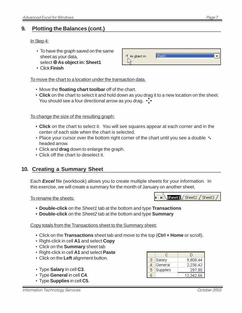
In Step 4:

• To have the graph saved on the same sheet as your data, select As object in: Sheet1

• Click Finish

To move the chart to a location under the transaction data.

• Move the floating chart toolbar off of the chart. • Click on the chart to select it and hold down as you drag it to a new location on the sheet.

You should see a four directional arrow as you drag.

To change the size of the resulting graph:

• Click on the chart to select it. You will see squares appear at each corner and in the center of each side when the chart is selected.

• Place your cursor over the bottom right corner of the chart until you see a double headed arrow.

• Click and drag down to enlarge the graph. • Click off the chart to deselect it.

10. Creating a Summary Sheet

Each Excel file (workbook) allows you to create multiple sheets for your information. In this exercise, we will create a summary for the month of January on another sheet.

To rename the sheets:

• Double-click on the Sheet1 tab at the bottom and type Transactions • Double-click on the Sheet2 tab at the bottom and type Summary

Copy totals from the Transactions sheet to the Summary sheet:

• Click on the Transactions sheet tab and move to the top (Ctrl + Home or scroll). • Right-click in cell A1 and select Copy • Click on the Summary sheet tab • Right-click in cell A1 and select Paste • Click on the Left alignment button.

• Type Salary in cell C3. • Type General in cell C4. • Type Supplies in cell C5.



10. Creating a Summary Sheet (cont.)

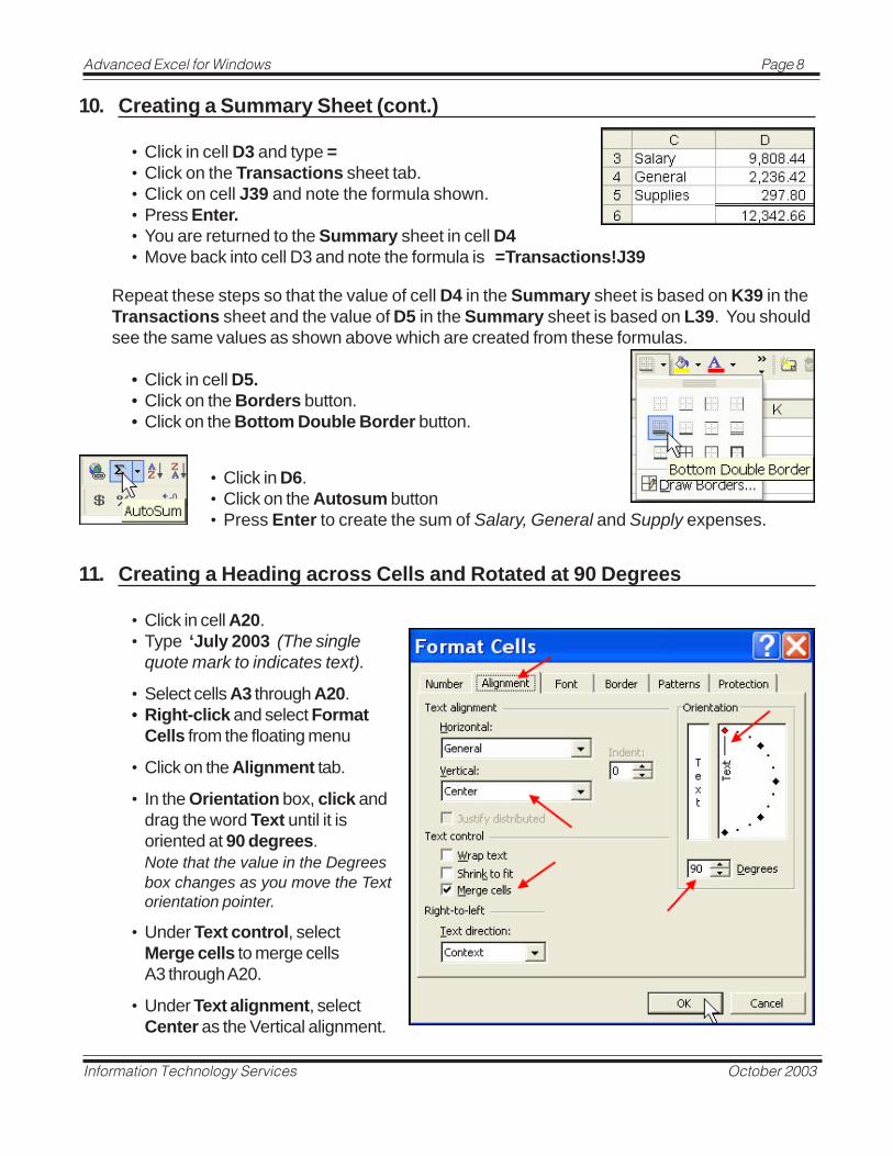
• Click in cell D3 and type = • Click on the Transactions sheet tab. • Click on cell J39 and note the formula shown. • Press Enter. • You are returned to the Summary sheet in cell D4 • Move back into cell D3 and note the formula is =Transactions!J39

Repeat these steps so that the value of cell D4 in the Summary sheet is based on K39 in the Transactions sheet and the value of D5 in the Summary sheet is based on L39. You should see the same values as shown above which are created from these formulas.

• Click in cell D5. • Click on the Borders button. • Click on the Bottom Double Border button.

• Click in D6. • Click on the Autosum button • Press Enter to create the sum of Salary, General and Supply expenses.

11. Creating a Heading across Cells and Rotated at 90 Degrees

• Click in cell A20. • Type ‘July 2003 (The single

quote mark to indicates text).

• Select cells A3 through A20. • Right-click and select Format

Cells from the floating menu

• Click on the Alignment tab.

• In the Orientation box, click and drag the word Text until it is oriented at 90 degrees. Note that the value in the Degrees box changes as you move the Text orientation pointer.

• Under Text control, select Merge cells to merge cells A3 through A20.

• Under Text alignment, select Center as the Vertical alignment.



11. Creating a Heading across Cells and Rotated at 90 Degrees (cont.)

• Click on the Font tab. • Select Bold as the Font style. • Select 24 as the font Size.

• Click on the Patterns tab. • Select a medium yellow. • Click OK.

12. Formatting a Heading

To format the heading American Travel Expenses:

• Select cells A1 through F1. • Click on the Merge and Center button.

• Click on the Bold formatting button. • Click on the Font Size down arrow and select 20 from the pulldown menu.

• Click on the Fill Color button to set a background color for the heading.

• Select Sky Blue.

13. Creating a Pie Chart on the Summary Sheet

• Select the numbers to be used in the chart by highlighting C3 to D5. • Click on the Chart Wizard button. • Under Chart type: select Pie. • Under Chart sub-type,

select the second style. • Click Next. • Click Next. • Select the Legend tab. • Click to deselect Show Legend.



13. Creating a Pie Chart on the Summary Sheet (cont.)

• Select the Data Labels tab. • Select Category name and Percentage. • Click Finish to complete the chart and skip step 4, accepting

the default to place the chart on the same sheet as your data.

To move and resize the pie chart:

• Click on the pie chart to select it and hold down as you drag it to directly under row 6. You should see a four directional arrow as you drag.

• With the pie chart still selected, place the cursor over the bottom right corner of the chart until a double headed arrow appears.

• Click and drag down to cell G23.

• With the chart still selected, right-click. • Select Format Chart Area from the floating menu. • Under the Patterns tab, select None for the Border.

14. The Final Summary Sheet



15. Printing and Exiting

• Select File Print. • Note that you may print the Entire workbook,

a Selection, or the Active sheet.

• To print just the chart, select the chart by clicking on it near the edge and then select File Print. Note that Selected Chart is indicated under Print what.

To exit the program:

• Select File Exit or use the close box in the upper right corner.

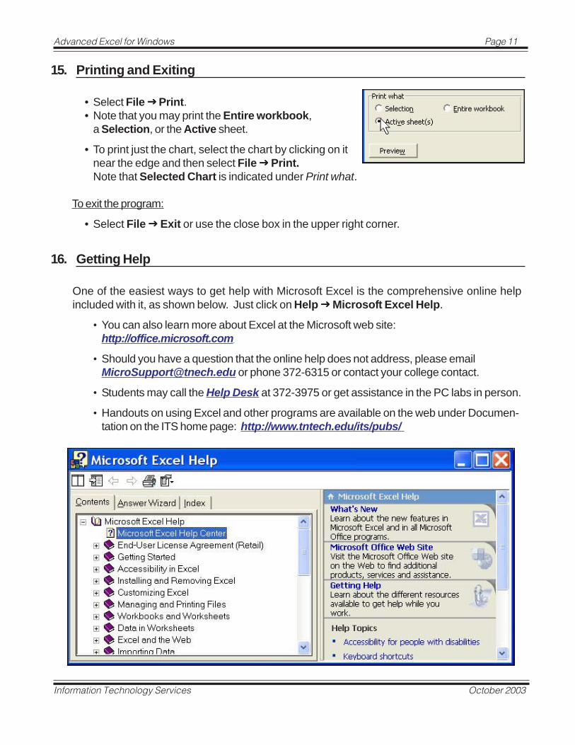
16. Getting Help

One of the easiest ways to get help with Microsoft Excel is the comprehensive online help included with it, as shown below. Just click on Help Microsoft Excel Help.

• You can also learn more about Excel at the Microsoft web site: http://office.microsoft.com

• Should you have a question that the online help does not address, please email [email protected] or phone 372-6315 or contact your college contact.

• Students may call the Help Desk at 372-3975 or get assistance in the PC labs in person.

• Handouts on using Excel and other programs are available on the web under Documen-tation on the ITS home page: http://www.tntech.edu/its/pubs/

http://office.microsoft.com

mailto:[email protected]

http://www.tntech.edu/helpdesk/

http://www.tntech.edu/its/pubs/



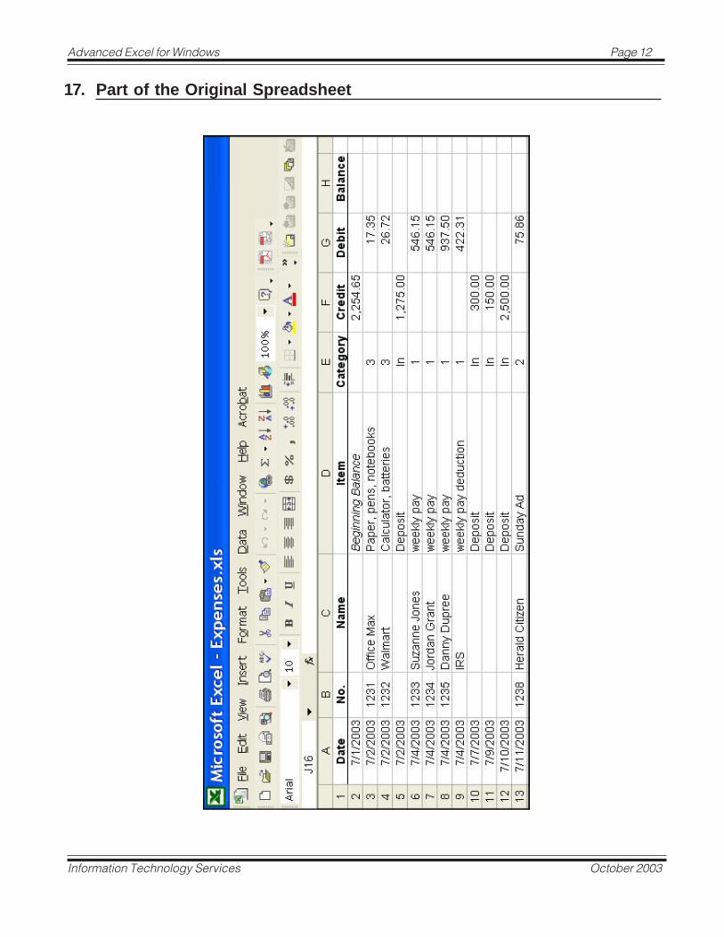
17. Part of the Original Spreadsheet