advanced model-order reduction techniques for … model order reduction (mor) has proven to be a...
TRANSCRIPT

Advanced Model-Order Reduction Techniques forLarge-Scale Dynamical Systems
by
Seyed-Behzad Nouri, B.Sc., M.A.Sc.
A thesis submitted to the Faculty of Graduate and PostdoctoralAffairs in partial fulfilment of the requirements
for the degree of
Doctor of Philosophyin
Electrical and Computer Engineering
Ottawa-Carleton Institute for Electrical and Computer Engineering
Department of Electronics
Carleton University
Ottawa, Ontario, Canada
© 2014Seyed-Behzad Nouri

Abstract
Model Order Reduction (MOR) has proven to be a powerful and necessary tool for various
applications such as circuit simulation. In the context of MOR, there are some unaddressed
issues that prevent its efficient application, such as “reduction of multiport networks” and
“optimal order estimation” for both linear and nonlinear circuits. This thesis presents the
solutions for these obstacles to ensure successful model reduction of large-scale linear and
nonlinear systems.
This thesis proposes a novel algorithm for creating efficient reduced-order macromodels
from multiport linear systems (e.g. massively coupled interconnect structures). The new
algorithm addresses the difficulties associated with the reduction of networks with large
numbers of input/output terminals, that often result in large and dense reduced-order mod-
els. The application of the proposed reduction algorithm leads to reduced-order models
that are sparse and block-diagonal in nature. It does not assume any correlation between
the responses at ports; and thereby overcomes the accuracy degradation that is normally as-
sociated with the existing (Singular Value Decomposition based) terminal reduction tech-
niques.
Estimating an optimal order for the reduced linear models is of crucial importance to ensure
accurate and efficient transient behavior. Order determination is known to be a challenging
task and is often based on heuristics. Guided by geometrical considerations, a novel and
efficient algorithm is presented to determine the minimum sufficient order that ensures the
ii

accuracy and efficiency of the reduced linear models.
The optimum order estimation for nonlinear MOR is extremely important. This is mainly
due to the fact that, the nonlinear functions in circuit equations should be computed in the
original size within the iterations of the transient analysis. As a result, ensuring both ac-
curacy and efficiency becomes a cumbersome task. In response to this reality, an efficient
algorithm for nonlinear order determination is presented. This is achieved by adopting the
geometrical approach to nonlinear systems, to ensure the accuracy and efficiency in tran-
sient analysis.
Both linear and nonlinear optimal order estimation methods are not dependent on any spe-
cific order reduction algorithm and can work in conjunction with any intended reduced
modeling technique.
iii

Dedicated:To the living memories of my father, who lived by example to
inspire and motivate his students and children. I also dedicate
this to my mother, my understanding wife, and my wonderful
sons Ali and Ryan for their endless love, support, and encour-
agements.
iv

Acknowledgments
First and foremost, I would sincerely like to express my gratitude to my supervisor, Pro-
fessor Michel Nakhla. Without his guidance, this thesis would have been impossible. I
appreciate his insight into numerous aspects of numerical simulation and circuit theory, as
well as his enthusiasm, wisdom, care and attention. I have learned from him many aspects
of science and life. Working with him was truly an invaluable experience.
I am also sincerely grateful to to my co-supervisor, Professor RamAchar, for his helpful
suggestions and guidance, which was crucial in many stages of the research for this thesis.
Most of all I wish to thank him for his motivation and encouragements.
I would like to thank my current and past fellow colleagues in our Computer-Aided
Design group for keeping a spirit of collaboration and mutual respect. They were always
readily available for some friendly deliberations that made my graduate life enjoyable. I
will always fondly remember their support and friendship.
I am thankful towards the staff of the Department of Electronics at Carleton University
for having been so helpful, supportive, and resourceful.
Last but not least, I give special thanks to my family for all their unconditional love,
encouragement, and support. I am eternally indebted to my wife and both my sons for their
unconditional, invaluable and relentless support, encouragement, patience and respect. I
would like to thank Mrs Zandi for all her understandings and gracious friendship with my
v

family. My final thoughts are with my parents to whom I am forever grateful. I cherish the
memories of my late father with great respect. Words cannot express my admiration for the
endless kindness, dedication, and sacrifices that my parents have made for their children.
I believe that I could not have achieved this without their unlimited sacrifice. This is for
them.
Thank you all sincerely,
vi

Table of Contents
Abstract ii
Acknowledgments v
Table of Contents vii
List of Tables xiii
List of Figures xiv
List of Acronyms xx
List of Symbols xxii
Introduction 1
1 Background and Preliminaries 6
1.1 Dynamical Systems . . . . . . . . . . . . . . . . . . . . . . . . . . . . . . 6
1.2 Linear Systems . . . . . . . . . . . . . . . . . . . . . . . . . . . . . . . . 7
1.2.1 Important Property of Linear Systems . . . . . . . . . . . . . . . . 9
1.2.2 Mathematical Modeling of Linear Systems . . . . . . . . . . . . . 10
vii

1.3 Nonlinear Systems . . . . . . . . . . . . . . . . . . . . . . . . . . . . . . 13
1.3.1 Solutions of Nonlinear Systems . . . . . . . . . . . . . . . . . . . 15
1.3.2 Linear versus Nonlinear . . . . . . . . . . . . . . . . . . . . . . . 16
1.4 Mathematical Modeling of Electrical Networks . . . . . . . . . . . . . . . 16
1.5 Overview of Formulation of Circuit Dynamics . . . . . . . . . . . . . . . . 18
1.5.1 MNA Formulation of Linear Circuits . . . . . . . . . . . . . . . . 19
1.5.2 MNA Formulation of Nonlinear Circuits . . . . . . . . . . . . . . . 20
2 Model Order Reduction - Basic Concepts 25
2.1 Motivation . . . . . . . . . . . . . . . . . . . . . . . . . . . . . . . . . . . 26
2.2 The General Idea of Model Order Reduction . . . . . . . . . . . . . . . . . 26
2.3 Model Accuracy Measures . . . . . . . . . . . . . . . . . . . . . . . . . . 28
2.3.1 Error in Frequency Domain . . . . . . . . . . . . . . . . . . . . . 31
2.4 Model Complexity Measures . . . . . . . . . . . . . . . . . . . . . . . . . 32
2.5 Main Requirements for Model Reduction Algorithms . . . . . . . . . . . . 33
2.6 Essential Characteristic of Physical Systems . . . . . . . . . . . . . . . . . 34
2.6.1 Stability of Dynamical Systems . . . . . . . . . . . . . . . . . . . 34
2.6.2 Internal Stability . . . . . . . . . . . . . . . . . . . . . . . . . . . 35
2.6.3 External Stability . . . . . . . . . . . . . . . . . . . . . . . . . . . 38
2.6.4 Passivity of a Dynamical Model . . . . . . . . . . . . . . . . . . . 38
2.7 The Need for MOR for Electrical Circuits . . . . . . . . . . . . . . . . . . 39
3 Model Order Reduction for Linear Dynamical Systems 40
viii
3.1 Physical Properties of Linear Dynamical Systems . . . . . . . . . . . . . . 41
3.1.1 Stability of Linear Systems . . . . . . . . . . . . . . . . . . . . . . 41
3.1.2 Passivity of Linear Systems . . . . . . . . . . . . . . . . . . . . . 46
3.2 Linear Order Reduction Algorithms . . . . . . . . . . . . . . . . . . . . . 49
3.3 Polynomial Approximations of Transfer Functions . . . . . . . . . . . . . 50
3.3.1 AWE Based on Explicit Moment Matching . . . . . . . . . . . . . 52
3.4 Projection-Based Methods . . . . . . . . . . . . . . . . . . . . . . . . . . 53
3.4.1 General Krylov-Subspace Methods . . . . . . . . . . . . . . . . . 56
3.4.2 Truncated Balance Realization (TBR) . . . . . . . . . . . . . . . . 58
3.4.3 Proper Orthogonal Decomposition (POD) Methods . . . . . . . . . 64
3.5 Non-Projection Based MOR Methods . . . . . . . . . . . . . . . . . . . . 67
3.5.1 Hankel Optimal Model Reduction . . . . . . . . . . . . . . . . . . 67
3.5.2 Singular Perturbation . . . . . . . . . . . . . . . . . . . . . . . . . 67
3.5.3 Transfer Function Fitting Method . . . . . . . . . . . . . . . . . . 68
3.6 Other Alternative Methods . . . . . . . . . . . . . . . . . . . . . . . . . . 76
4 Model Order Reduction for Nonlinear Dynamical Systems 77
4.1 Physical Properties of Nonlinear Dynamical Systems . . . . . . . . . . . . 78
4.1.1 Lipschitz Continuity . . . . . . . . . . . . . . . . . . . . . . . . . 79
4.1.2 Existence and Uniqueness of Solutions . . . . . . . . . . . . . . . 80
4.1.3 Stability of Nonlinear Systems . . . . . . . . . . . . . . . . . . . . 81
4.2 Nonlinear Order Reduction Algorithms . . . . . . . . . . . . . . . . . . . 84
4.2.1 Projection framework for Nonlinear MOR - Challenges . . . . . . . 84
ix

4.2.2 Nonlinear Reduction Based on Taylor Series . . . . . . . . . . . . 86
4.2.3 Piecewise Trajectory based Model Order Reduction . . . . . . . . . 91
4.2.4 Proper Orthogonal Decomposition (POD) Methods . . . . . . . . . 95
4.2.5 Empirical Balanced Truncation . . . . . . . . . . . . . . . . . . . 98
4.2.6 Summary . . . . . . . . . . . . . . . . . . . . . . . . . . . . . . . 100
5 Reduced Macromodels of Massively Coupled Interconnect Structures via
Clustering 101
5.1 Introduction . . . . . . . . . . . . . . . . . . . . . . . . . . . . . . . . . . 101
5.2 Background and Preliminaries . . . . . . . . . . . . . . . . . . . . . . . . 104
5.2.1 Formulation of Circuit Equations . . . . . . . . . . . . . . . . . . 105
5.2.2 Model-Order Reduction via Projection . . . . . . . . . . . . . . . . 106
5.3 Development of the Proposed Algorithm . . . . . . . . . . . . . . . . . . . 107
5.3.1 Formulation of Submodels Based on Clustering . . . . . . . . . . . 108
5.3.2 Formulation of the Reduced Model Based on Submodels . . . . . . 110
5.4 Properties of the Proposed Algorithm . . . . . . . . . . . . . . . . . . . . 114
5.4.1 Preservation of Moments . . . . . . . . . . . . . . . . . . . . . . . 114
5.4.2 Stability . . . . . . . . . . . . . . . . . . . . . . . . . . . . . . . . 115
5.4.3 Passivity . . . . . . . . . . . . . . . . . . . . . . . . . . . . . . . 116
5.4.4 Guideline for Clustering to Improve Passivity . . . . . . . . . . . . 123
5.5 Numerical Examples . . . . . . . . . . . . . . . . . . . . . . . . . . . . . 125
5.5.1 Example I . . . . . . . . . . . . . . . . . . . . . . . . . . . . . . . 126
5.5.2 Example II . . . . . . . . . . . . . . . . . . . . . . . . . . . . . . 130
x

6 Optimum Order Estimation of Reduced Linear Macromodels 136
6.1 Introduction . . . . . . . . . . . . . . . . . . . . . . . . . . . . . . . . . . 136
6.2 Development of the Proposed Algorithm . . . . . . . . . . . . . . . . . . . 137
6.2.1 Preliminaries . . . . . . . . . . . . . . . . . . . . . . . . . . . . . 137
6.2.2 Geometrical Framework for the Projection . . . . . . . . . . . . . 140
6.2.3 Neighborhood Preserving Property . . . . . . . . . . . . . . . . . . 142
6.2.4 Unfolding the Projected Trajectory . . . . . . . . . . . . . . . . . . 148
6.3 Computational Steps of the Proposed Algorithm . . . . . . . . . . . . . . . 150
6.4 Numerical Examples . . . . . . . . . . . . . . . . . . . . . . . . . . . . . 153
6.4.1 Example I . . . . . . . . . . . . . . . . . . . . . . . . . . . . . . . 153
6.4.2 Example II . . . . . . . . . . . . . . . . . . . . . . . . . . . . . . 156
7 Optimum Order Determination for Reduced Nonlinear Macromodels 162
7.1 Introduction . . . . . . . . . . . . . . . . . . . . . . . . . . . . . . . . . . 162
7.2 Background . . . . . . . . . . . . . . . . . . . . . . . . . . . . . . . . . . 163
7.2.1 Formulation of Nonlinear Circuit Equations . . . . . . . . . . . . . 163
7.2.2 Model Order Reduction of Nonlinear Systems . . . . . . . . . . . . 164
7.2.3 Projection Framework . . . . . . . . . . . . . . . . . . . . . . . . 164
7.3 Order Estimation for Nonlinear Circuit Reduction . . . . . . . . . . . . . . 166
7.3.1 Differential Geometric Concept of Nonlinear Circuits . . . . . . . . 166
7.3.2 Nearest Neighbors . . . . . . . . . . . . . . . . . . . . . . . . . . 172
7.3.3 Geometrical Framework for the Projection . . . . . . . . . . . . . 173
7.3.4 Proposed Order Estimation for Nonlinear Reduced Models . . . . . 175
xi

7.4 Computational Steps of the Proposed Algorithm . . . . . . . . . . . . . . . 180
7.5 Numerical Examples . . . . . . . . . . . . . . . . . . . . . . . . . . . . . 185
7.5.1 Example I . . . . . . . . . . . . . . . . . . . . . . . . . . . . . . . 185
7.5.2 Example II . . . . . . . . . . . . . . . . . . . . . . . . . . . . . . 188
8 Conclusions and Future Work 196
8.1 Conclusions . . . . . . . . . . . . . . . . . . . . . . . . . . . . . . . . . . 196
8.2 Future Research . . . . . . . . . . . . . . . . . . . . . . . . . . . . . . . . 198
List of References 200
Appendix A Properties of Nonlinear Systems in Compare to Linear 226
Appendix B Model Order Reduction Related Concepts 228
B.1 Tools From Linear Algebra and Functional Analysis . . . . . . . . . . . . . 228
B.1.1 Review of Vector Space and Normed Space . . . . . . . . . . . . . 228
B.1.2 Review of the Different Norms . . . . . . . . . . . . . . . . . . . . 231
B.2 Mappings Concepts . . . . . . . . . . . . . . . . . . . . . . . . . . . . . . 232
Appendix C Proof of Theorem-5.1 in Section 5.4 238
Appendix D Proof of Theorem-5.2 in Section 5.4 244
xii

List of Tables
1.1 Summary: general properties of linear and nonlinear systems . . . . . . . . 17
2.1 Measuring reduction accuracy in time domain . . . . . . . . . . . . . . . . 30
3.1 Time complexities of standard TBR. . . . . . . . . . . . . . . . . . . . . . 61
4.1 Comparison of properties of the available nonlinear model order reduction
algorithm . . . . . . . . . . . . . . . . . . . . . . . . . . . . . . . . . . . 100
5.1 CPU-cost comparison between original system, PRIMA and proposed
method. . . . . . . . . . . . . . . . . . . . . . . . . . . . . . . . . . . . . 129
xiii

List of Figures
1.1 Illustration of linear physical system L. . . . . . . . . . . . . . . . . . . . 8
1.2 Illustration of a subcircuit that accepting p-inputs and interacting with other
module trough its q-outputs. . . . . . . . . . . . . . . . . . . . . . . . . . 21
2.1 Model order reduction. . . . . . . . . . . . . . . . . . . . . . . . . . . . . 29
2.2 Measuring error of approximation. . . . . . . . . . . . . . . . . . . . . . . 29
3.1 Illustrates the uniform stability; uniformity implies the σ-bound is indepen-
dent of t0. . . . . . . . . . . . . . . . . . . . . . . . . . . . . . . . . . . . 43
3.2 A decaying-exponential bound independent of t0. . . . . . . . . . . . . . . 44
4.1 Illustration of Lipschitz property. . . . . . . . . . . . . . . . . . . . . . . . 80
4.2 Model reduction methods for nonlinear dynamical systems categorized into
four classes. . . . . . . . . . . . . . . . . . . . . . . . . . . . . . . . . . . 84
4.3 Illustration of the state space of a planar system, where xi are the expansion
points on the training trajectory A. Because solutions B and C are in the
vicinity ball of the expansion states, they can be efficiently simulated using
a TPWL model, however this can not be true for the solutions D and E. . . . 92
4.4 Nonlinear Balanced model reduction. . . . . . . . . . . . . . . . . . . . . 99
xiv

5.1 Reduced-modeling of multiport linear networks representing N -conductor
TL. . . . . . . . . . . . . . . . . . . . . . . . . . . . . . . . . . . . . . . 108
5.2 Illustration of forming clusters of active and victim lines in a multiconduc-
tor transmission line system. . . . . . . . . . . . . . . . . . . . . . . . . . 109
5.3 Linear (RLC) subcircuit π accompanied with the reduced model Ψ. . . . . 112
5.4 The overall network comprising the reduced model, embedded RLC sub-
circuit, and nonlinear termination. . . . . . . . . . . . . . . . . . . . . . . 113
5.5 Illustration of strongly coupled lines bundled together as active lines in the
clusters. . . . . . . . . . . . . . . . . . . . . . . . . . . . . . . . . . . . . 118
5.6 The frequency-spectrum of the minimum eigenvalue ofΦ(s) containing 32
clusters. . . . . . . . . . . . . . . . . . . . . . . . . . . . . . . . . . . . . 124
5.7 The enlarged region near the x-axis of Fig. 5.6 (illustrating eigenvalues
extending to the negative region, indicating passivity violation). . . . . . . 125
5.8 Spectrum of Φ(s) versus frequency with proper clustering to improve pas-
sivity (no passivity violations observed). . . . . . . . . . . . . . . . . . . . 126
5.9 The frequency-spectrum of the minimum eigenvalue of Φ(s) with cluster-
ing to improve passivity behavior (no passivity violations observed). . . . . 127
5.10 32 conductor coupled transmission line network with terminations consid-
ered in the example. . . . . . . . . . . . . . . . . . . . . . . . . . . . . . . 128
5.11 Sparsity pattern of reduced MNA equations using conventional PRIMA
(dense). . . . . . . . . . . . . . . . . . . . . . . . . . . . . . . . . . . . . 129
5.12 Sparsity pattern of reduced MNA equations using the proposed method. . . 129
5.13 Transient responses at victim line near-end of line#2. . . . . . . . . . . . . 130
5.14 Transient responses at victim line near-end of line#12. . . . . . . . . . . . 131
xv

5.15 Transient responses at victim line far-end of line#31. . . . . . . . . . . . . 132
5.16 Cross sectional geometry (Example 2). . . . . . . . . . . . . . . . . . . . . 132
5.17 Interconnect structure with nine clusters (Example 2). . . . . . . . . . . . . 133
5.18 Minimum eigenvalue ofΦ(s) while using 9 clusters (each cluster with nine
lines while one of them acting as an active line). . . . . . . . . . . . . . . . 133
5.19 Negative eigenvalue of Φ(s) (using the 9-cluster approach). . . . . . . . . 134
5.20 Illustration of the interconnect structure grouped as three clusters (each
cluster with nine lines while the three of the strongly coupled lines in each
of them acting as active lines [shown in red color]). . . . . . . . . . . . . . 134
5.21 Eigenvalue of Φ(s) (using 3 clusters based on the proposed flexible clus-
tering approach). . . . . . . . . . . . . . . . . . . . . . . . . . . . . . . . 135
5.22 Minimum eigenvalues ofΦ(s) (using 3 clusters based on the proposed flex-
ible clustering approach). . . . . . . . . . . . . . . . . . . . . . . . . . . . 135
6.1 Any state corresponding to a certain time instant can be represented by a
point (e.g. A, N, E and F) on the trajectory curve (T) in the variable space. . 139
6.2 Illustration of a multidimensional adjacency ball centered at x(ti), accom-
modating its four nearest neighboring points. . . . . . . . . . . . . . . . . 141
6.3 Illustration of false nearest neighbor (FNN), where T is the projection of T
in Fig. 1. . . . . . . . . . . . . . . . . . . . . . . . . . . . . . . . . . . . . 142
6.4 Illustration of the neighborhood structure of the state xi and its projection
zi in the state space and reduced space, respectively. . . . . . . . . . . . . . 143
6.5 Displacement between two false nearest neighbors in the unfolding process. 149
6.6 (a) A lossy transmission line as a 2-port network with the terminations;
(b) Modeled by 1500 lumped RLGC π-sections in cascade. . . . . . . . . . 154
xvi

6.7 The percentage of the false nearest neighbors on the projected trajectory. . . 155
6.8 Transient response of the current entering to the far-end of the line when
the reduced model is of orderm = 66. . . . . . . . . . . . . . . . . . . . . 156
6.9 Transient response of the current at the far-end terminal of the line when
the reduced model is of orderm = 66. . . . . . . . . . . . . . . . . . . . . 157
6.10 Accuracy comparison in PRIMA models with different orders. . . . . . . . 158
6.11 A RLC mesh as a 24-port subcircuit with the terminations. . . . . . . . . . 158
6.12 The percentage of the false nearest neighbors among 1000 data points on
the projected trajectory. . . . . . . . . . . . . . . . . . . . . . . . . . . . . 159
6.13 Transient responses at near-end of horizontal trace#1. . . . . . . . . . . . . 160
6.14 Transient responses at near-end of horizontal trace#10. . . . . . . . . . . . 160
6.15 Errors from using the reduced models with different orders in the frequency
domain. . . . . . . . . . . . . . . . . . . . . . . . . . . . . . . . . . . . . 161
7.1 Chua’s circuit. . . . . . . . . . . . . . . . . . . . . . . . . . . . . . . . . . 167
7.2 Trajectory of the Chua’s circuit in the state-space (scaled time: 0 ≤ t ≤100) for a given initial condition. . . . . . . . . . . . . . . . . . . . . . . . 167
7.3 The time-series plot of the system variables (xi(t)) as coordinates of state
space. . . . . . . . . . . . . . . . . . . . . . . . . . . . . . . . . . . . . . 168
7.4 (a) Digital inverter circuit; (b) The circuit model to characterize the dy-
namic behavior of digital inverter at its ports. . . . . . . . . . . . . . . . . 169
7.5 A geometric structureM attracting the trajectories of the circuit in Fig.7.4. 169
7.6 (a) The Möbus strip and (b) Torus are visualizations of 2D manifolds in R3 170
xvii

7.7 Illustration of a multidimensional adjacency ball centered at x(ti) (✕), ac-
commodating its two nearest neighboring points (▼) on the trajectory of
the Chua’s circuit (for 0 ≤ t ≤ 2). . . . . . . . . . . . . . . . . . . . . . . 172
7.8 Illustration of Chua’s trajectory in Fig.7.7 projected to a two-dimensional
subspace, where its underlying manifold is over-contracted. . . . . . . . . . 174
7.9 (left) Illustration of false nearest neighbor (FNN), where the 3-dimensional
trajectory of the Chua’s circuit in Fig.7.7 is projected; (right) A zoomed-in
view of the projected trajectory. . . . . . . . . . . . . . . . . . . . . . . . 174
7.10 Drastic displacement between two false nearest neighbors in the unfolding
process. . . . . . . . . . . . . . . . . . . . . . . . . . . . . . . . . . . . . 176
7.11 Small displacement between every two nearest neighbors by adding a new
dimension (m + 1 or higher), when trajectory was fully unfolded in m
dimensional space. . . . . . . . . . . . . . . . . . . . . . . . . . . . . . . 177
7.12 Flowchart of the proposed nonlinear order estimation strategy. The gray
blocks are the steps of nonlinear MOR interacting with the proposed methods.182
7.13 (a) Diode chain circuit, (b) Excitation waveform at input. . . . . . . . . . . 186
7.14 The percentage of the false nearest neighbors on the projected nonlinear
trajectory. . . . . . . . . . . . . . . . . . . . . . . . . . . . . . . . . . . . 187
7.15 Accuracy comparison in the reduced models with different orders (left y-
axis) along with the FNN (%) on the projected nonlinear trajectories (right
y-axis). . . . . . . . . . . . . . . . . . . . . . . . . . . . . . . . . . . . . 188
7.16 Excitation test waveform at input and comparison of the responses at
nodes 3, 5 and 7, respectively. . . . . . . . . . . . . . . . . . . . . . . . . 189
xviii

7.17 (a) Nonlinear transmission line circuit model, (b) Excitation waveform at
input. . . . . . . . . . . . . . . . . . . . . . . . . . . . . . . . . . . . . . 190
7.18 The percentage of the false nearest neighbors on the projected nonlinear
trajectory. . . . . . . . . . . . . . . . . . . . . . . . . . . . . . . . . . . . 191
7.19 Accuracy comparison in the reduced models with different orders (left y-
axis) along with the FNN (%) on the projected nonlinear trajectories (right
y-axis). . . . . . . . . . . . . . . . . . . . . . . . . . . . . . . . . . . . . 192
7.20 (a) Excitation test waveform at input, (b) Comparison of the responses at
nodes 5, 50, 70, and 200, respectively. . . . . . . . . . . . . . . . . . . . . 193
7.21 Excitation waveform at input. . . . . . . . . . . . . . . . . . . . . . . . . . 193
7.22 The percentage of the false nearest neighbors on the projected nonlinear
trajectory. . . . . . . . . . . . . . . . . . . . . . . . . . . . . . . . . . . . 194
7.23 Accuracy comparison in the reduced models with different orders (left y-
axis) along with the FNN (%) on the projected nonlinear trajectories (right
y-axis). . . . . . . . . . . . . . . . . . . . . . . . . . . . . . . . . . . . . 194
7.24 Comparison of the responses at output nodes for the segments 30, 60 and
70 respectively. . . . . . . . . . . . . . . . . . . . . . . . . . . . . . . . . 195
B.1 Visualization of a mapping . . . . . . . . . . . . . . . . . . . . . . . . . . 233
B.2 Visualization of an injective mapping . . . . . . . . . . . . . . . . . . . . 234
B.3 Visualization of an surjective mapping . . . . . . . . . . . . . . . . . . . . 234
B.4 Inverse mapping T−1 : Y −→ D (T) ⊆ X of a bijective mapping T . . . . 235
xix

List of Acronyms
Acronyms Definition
ADE Algebraic Differential Equation
AWE Asymptotic Waveform Evaluation
BIBO Bounded-In Bounded-Out
CAD Computer Aided Design
CPU Central Processing Unit
DAE Differential-Algebraic Equation
EIG Eigenvalue (diagonal) Decomposition
FD Frequency Domain
FNN False Nearest Neighbor
HSV Hankel Singular Value
IC Integrated Circuit
I/O Input-Output
KCL Kirchoff’s Current Law
KVL Kirchoff’s Voltage Law
LHP Left Half (of the complex) Plane
LHS Left Hand Side
LTI Linear Time Invariant (Dynamical System)
MEMS Micro-Electro-Mechanical System
MIMO Multi Input and Multi Output (multiport) system
MOR Model Order Reduction
xx
NN Nearest Neighboring point
ODE Ordinary Differential Equation
PDE Partial Differential Equation
POD Proper Orthogonal Decomposition
PRIMA Passive Reduced-order Interconnect Macromodeling Algorithm
PVL Padé Via Lanczos
RHP Right Half (of the complex) Plane
RHS Right Hand Side
RMS Root Mean Square
SISO Single Input and Single Output system
SVD Singular Value Decomposition
TD Time Domain
TF Transfer Function
TBR Truncated Balanced Realization
TPWL Trajectory Piecewise Linear
VLSI Very Large Scale Integrated circuit
xxi

List of Symbols
Symbols Definition
N The field of natural numbers
R The field of real numbers
R+ The set of all positive real numbers
C The field of complex numbers, e.g.: s-plane
Rn The set of real column vectors of size n, Rn×1, i.e. n-dimensional
Euclidean space
Cn The set of complex column vectors of size n, Cn×1, i.e. n-dimensional
Euclidean space
Rn×m The set of real matrices of size n×m
Cn×m The set of complex matrices of size n×m
C+ The open right half plane in the complex plane; C+ = {s ∈ C : �(s) > 0}C− The open left half plane in the complex plane; C− = {s ∈ C : �(s) < 0}C+ The closed right half plane in the complex plane; C+ = {s ∈ C : �(s) ≥ 0}C− The closed left half plane in the complex plane; C− = {s ∈ C : �(s) ≤ 0}� or �e Real part of a complex number
� or �m Imaginary part of a complex number
Cn n differentiable (n-smooth)
C∞ Infinitely differentiable (smooth)
a or a∗ The complex conjugate of a complex number a ∈ C
xxii

Am×n Anm× n matrixA = [aij], where aij is an element in i-th row and j-th column
AT The transpose of matrixA = [aij], defined asAT = [aji]
A orA∗ Complex-conjugate of each entries in complex matrixA = [aij], defined as:
A∗ = A = [aij ]
AH Complex-conjugate transpose of complex matrixA = [aij], defined as:
AH = AT= [aji]
In An n× n identity matrix I =[ıij
], where ıij = 1, for i = j and
ıij = 0, for i �= j
A−1n×n The inverse of the square matrixA such thatA−1 A = AA−1 = In
∅∅∅ Empty set / empty subspace
det (A) Determinant of matrixA
rank (A) Rank of matrixA
dim (A) Dimension of an square matrixA ∈ Cn×n, e.g. dim (A) = n
A > 0 A is a positive definite matrix
A ≥ 0 A is a semi-positive definite matrix
colsp (A) Column span (also called range) of matrixA
λ (A) Set of eigenvalues (spectrum) of square matrixA
λi (A) i-th eigenvalue of matrixA
λmax (A) Maximum eigenvalue of matrixA, the largest eigenvalue in the spectrum ofA
λmin (A) Minimum eigenvalue of matrixA, the smallest eigenvalue in the set
σ (A) Set of singular values of matrixA
σi (A) i-th singular value of matrixA
σmax (A) Maximum singular values of matrixA, i.e. = σ1
σmin (A) Minimum singular values of matrixA, i.e. = σn
λ (E, A) Set of all finite eigenvalues of the regular matrix pencil (E,A)⌊q/p
⌋m = max
(q
p
)| m ∈ N
span (x1,x2, . . . ,xn) Vector space spanned by the vectors x1,x2, . . . ,xn
diag(d1, d2, . . . , dn) Diagonal matrix with d1, d2, . . . , dn on its diagonal
blkdiag {A1, . . . ,Ak} Block diagonal matrix with the blocksA1, . . . ,An on its diagonal
xxiii

deg( ) Degree of polynomials with real/complex coefficients
sup { } Supremum of a set
‖x‖ Euclidean vector norm x ∈ Cn, ‖x‖ =
(∑i
x2i
) 12
‖A‖ The consistent matrix norm subordinate to Euclidean vector norm, i.e.
maxx∈Rn−{0}
‖Ax‖‖x‖ = σmax (A)
‖A‖F Frobenius norm of matrixA ∈ Cm×n, i.e.
(m∑i=1
n∑j=1
|aij|2)1/2
=
(n∑
i=1
σi
)1/2
,
given n ≤ m
‖A‖1 Maximum of the sum of column vectors in matrixA ∈ Cm×n, i.e. max
1≤j≤n
m∑i=1
|aij|
‖A‖∞ Maximum of the sum of row vectors in matrixA, i.e. max1≤i≤m
n∑j=1
|aij|
s Complex frequency (Laplace variable), s = α + jω, α, ω ∈ R
∀ For all
∃, ∃! There exist, there exists exactly one (uniqueness)
∈, /∈ Is an element of, is not an element of
⊆, �→ Sub-set, maps to
: or | Such that
iff If and only ifΔ=,
def= Equals by definition, is defined as
A⊗B =
⎡⎢⎢⎣a11B . . . a1mB... . . . ...
an1B . . . anmB
⎤⎥⎥⎦ Kronecker product of matricesA ∈ Cn,m and B
xxiv
Introduction
Signal and power integrity analysis of high-speed interconnects and packages are becom-
ing increasingly important. However, they have become extremely challenging due to the
large circuit sizes and mixed frequency-time domain analysis issues. The circuit equations,
despite being large, are fortunately extremely sparse. Exploiting sparsity lowers the com-
putational cost associated with the application of numerical techniques on circuit equations.
However, after some level of complexity and scale, the simulation of circuits in their origi-
nal size is prohibitively expensive. Model order reduction (MOR) has proven successful in
tackling this reality and hence, has been an active research topic in the CAD area. The goal
of MOR is to extract a smaller but accurate model for a given system, in order to accelerate
simulations of large complex designs. In order to preserve the accuracy of these downsized
models over a large bandwidth, the order of the resulting macromodels may end up being
high. On the other hand, any attempt of reduction can drastically impair the sparsity of the
original system. The large number of ports even worsen the problem of being high-order
and dense. Particularly, reduction of the circuit equations for electrical networks with large
number of input/output terminals often leads to very large and dense reduced models. It is
to be noted that, as the number of ports of a circuit increases (e.g. in the case of large bus
structures), the size of reduced models also grows proportionally. This degrades the effi-
ciency of transient simulations, significantly undermining the advantages gained by MOR
techniques.
1

So far, MOR techniques for linear time invariant systems have been well-developed
and widely used. On the other hand, nonlinear systems present numerous challenges for
MOR. A common problem in the prominently used linear and nonlinear order-reduction
techniques is the “selection of proper order” for the reduced models. Determining the
“minimum” possible, yet “adequate” order is of critical importance to start the reduction
process. This ensures that the resulting model can still sufficiently preserve the impor-
tant physical properties of the original system. For both classes of physical systems, the
selection of an optimum order is important to achieve a pre-defined accuracy while not
over-estimating the order, which otherwise can lead to inefficient transient simulations and
hence, undermine the advantage from applying MOR.
This thesis presents solutions for the above obstacles to ensure successful model reduc-
tion of large-scale linear and nonlinear systems. For this purpose, it proposes an efficient
reduction algorithm to preserve the sparsity in the reduction of linear systems with large
number of ports. Furthermore, it presents the efficient algorithms to determine the optimum
order for linear and nonlinear macromodels.
Contributions
The main contributions of this thesis are as follows.
• A novel algorithm is developed for efficient reduction of linear networks with large
number of terminals. The new method, while exploiting the applicability of the su-
perposition paradigm for the analysis of massively coupled interconnect structures,
proposes a reduction strategy based on flexible clustering of the transmission lines
in the original network to form individual subsystems. The overall reduced model is
2
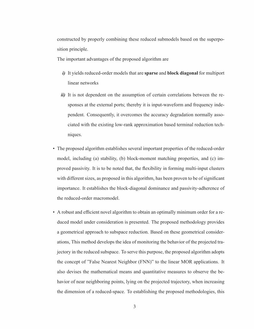
constructed by properly combining these reduced submodels based on the superpo-
sition principle.
The important advantages of the proposed algorithm are
i) It yields reduced-order models that are sparse and block diagonal for multiport
linear networks
ii) It is not dependent on the assumption of certain correlations between the re-
sponses at the external ports; thereby it is input-waveform and frequency inde-
pendent. Consequently, it overcomes the accuracy degradation normally asso-
ciated with the existing low-rank approximation based terminal reduction tech-
niques.
• The proposed algorithm establishes several important properties of the reduced-order
model, including (a) stability, (b) block-moment matching properties, and (c) im-
proved passivity. It is to be noted that, the flexibility in forming multi-input clusters
with different sizes, as proposed in this algorithm, has been proven to be of significant
importance. It establishes the block-diagonal dominance and passivity-adherence of
the reduced-order macromodel.
• A robust and efficient novel algorithm to obtain an optimally minimum order for a re-
duced model under consideration is presented. The proposed methodology provides
a geometrical approach to subspace reduction. Based on these geometrical consider-
ations, This method develops the idea of monitoring the behavior of the projected tra-
jectory in the reduced subspace. To serve this purpose, the proposed algorithm adopts
the concept of ”False Nearest Neighbor (FNN)” to the linear MOR applications. It
also devises the mathematical means and quantitative measures to observe the be-
havior of near neighboring points, lying on the projected trajectory, when increasing
the dimension of a reduced-space. To establishing the proposed methodologies, this
3

thesis exceeds beyond the extensive experimental justifications. It deeply contributes
to the theoretical aspects involved in these algorithms by establishing new concepts,
theorems and lemmas.
• A novel and efficient algorithm is developed to obtain the minimum sufficient order
that ensures the accuracy and efficiency of the reduced nonlinear model. The pro-
posed method, by deciding a proper order for the projected subspace, ensures that
the reduced model can inherit the dominant dynamical characteristics of the original
nonlinear system. The proposed method also adopts the concepts and mathematical
means from the False Nearest Neighbors (FNN) approach to trace the deformation of
nonlinear manifolds in the unfolding process. The proposed method is incorporated
into the projection basis generation algorithm to avoid the computational costs asso-
ciated with the extra basis. It is devised to be general enough to work in conjunction
with any intended nonlinear reduced modeling scheme such as: TPWL with a global
reduced subspace, TBR, or POD, etc.
As another important contribution, this thesis derives the bounds on the neighborhood
range (radius) when searching for the false neighbors. Bounding this neighborhood
range helps to enhance the efficiency of the automated algorithm by narrowing down
the range of possible choices for the threshold value in the ratio test.
Organization of the Thesis
This thesis is organized as follows.
Chapter 1 presents a concise background on the main subjects relevant to this work such as,
dynamical systems and their modelings as well as linear and nonlinear systems which are
studied from a comparative perspective. Chapter 2 reviews the general concept of MOR
4

and physical characteristics which should be preserved in the reduction process. The next
two chapters are of an introductory nature and provide an in-depth overview of the model
reduction methods for linear (Chapter 3 ) and nonlinear (Chapter 4) dynamical systems.
Next, Chapter 5 explains the details of the proposed methodologies for reduced macro-
modeling of massively coupled interconnect structures. In Chapter 6, a novel algorithm
for optimum order estimation is developed for reduced linear macromodels. This is fol-
lowed by Chapter 7, which presents a novel algorithm for optimum order determination
for reduced nonlinear models. Chapter 8 summarizes the proposed work and outlines the
direction of future research.
Appendix-A further compares the properties of nonlinear and linear systems. Appendix-
B presents some concepts from linear algebra and functional analysis that are useful for
studying the dynamic systems. Appendices C and D present the proofs for the theorems in
Chapter-5.
5

Chapter 1
Background and Preliminaries
This chapter presents a quick background on the main topics relevant to the subject of this
work. The main characteristics of general classes of both linear and nonlinear systems
are studied in a comparative manner. It also describes the groundwork for the electrical
networks and their properties as a (linear / nonlinear) dynamical system. In addition, an
overview of the formulation (mathematical modeling) for electrical networks is presented.
For the supplementary concepts and more details about the important nonlinear phenomena
Appendix A can also be referred to.
1.1 Dynamical Systems
A dynamical system is a system which changes in time according to some rule, law, or
"evolution equation". The intrinsic behavior of any dynamical system is defined based on
the following two elements [1],
(a) a rule or "dynamic", which specifies how a system evolves,
(b) an initial condition or "initial state" from which the system starts.
6

1.2. Linear Systems 7
The dynamical behavior of systems can be understood by studying their mathematical de-
scriptions. There are two main approaches to mathematically describe dynamical systems,
(a) differential equations (also referred to as “flows”),
(b) difference equations (also known as “iterated maps” or shortly “maps”).
Differential equations describe the evolution of systems in continuous time, whereas iter-
ated maps arise in problems where time is discrete [2, 3]. Differential equations are used
much more widely in electrical engineering, therefore we will focus on continuous-time
dynamical systems.
1.2 Linear Systems
In system theory (or functional analysis, or theory of operators), “linearity” is defined based
on the satisfaction of two properties, additivity and homogeneity, so called “superposition”
paradigm. For a given function (map) L and any inputs ui and uj additivity states that,
L(ui + uj) = L(ui) + L(uj), and homogeneity is L(ki ui) = ki L(ui), where ki is
any arbitrary real number. Hence, the following compact definition of linearity is generally
used:
L
(n∑
p=1
kp up
)=
n∑p=1
kp L (up), n ≥ 1, ∀ {kp} , {up} (Superposition) . (1.1)
Implicit in the above is the requirement that,
• For any linear function L (0) = 0
• For n = 1 i.e. homogeneity (the linear scaling), L (k u) = kL (u)
• L (ui − uj) = L (ui)−L (uj)
1.2. Linear Systems 8
• up for p = 1, . . . , n should be in the space of the possible inputs or the domain of the
function L. It is also required for the domain to be closed under linear combination;
i.e., ki ui + kj uj must belong to the domain if ui and uj do [4].
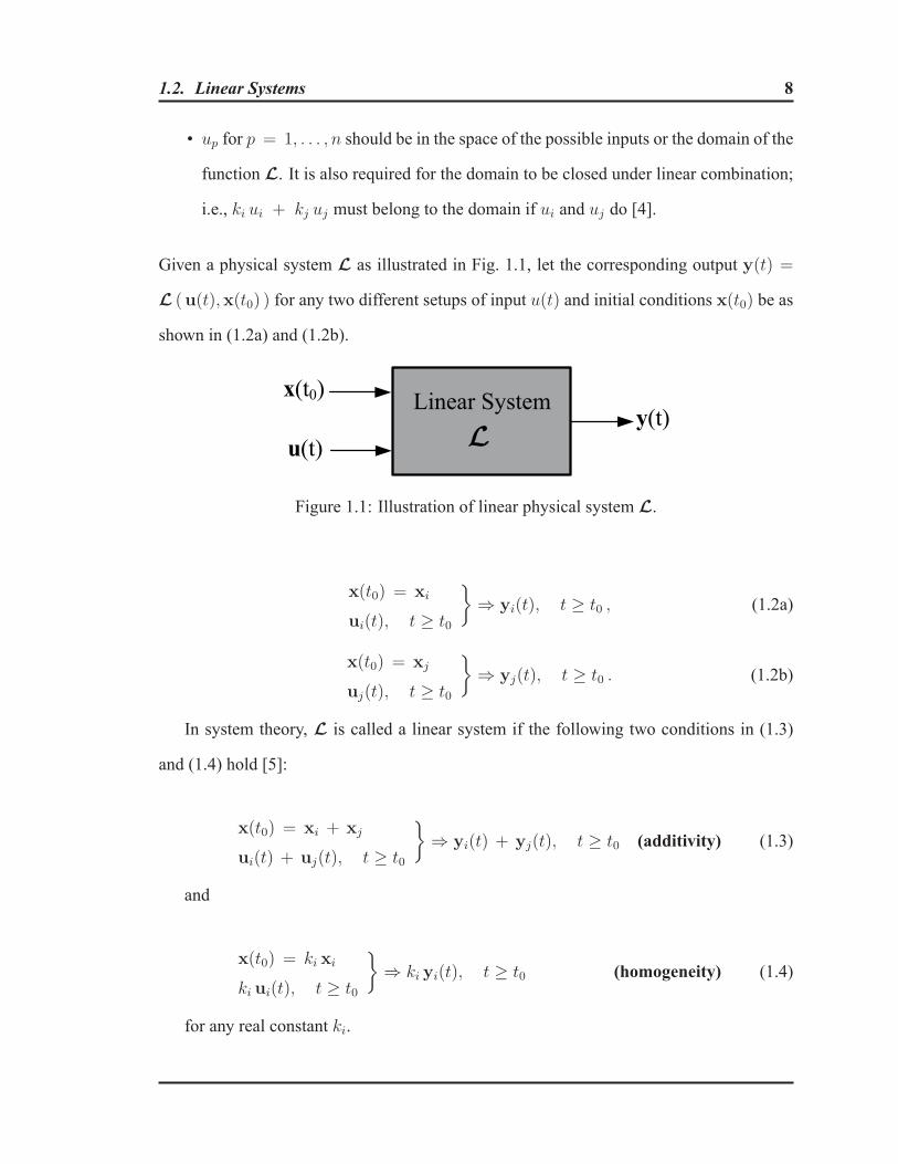
Given a physical system L as illustrated in Fig. 1.1, let the corresponding output y(t) =
L (u(t),x(t0) ) for any two different setups of input u(t) and initial conditions x(t0) be as
shown in (1.2a) and (1.2b).
u(t)
x(t0)
y(t)Linear System
Figure 1.1: Illustration of linear physical system L.
x(t0) = xi
ui(t), t ≥ t0
}⇒ yi(t), t ≥ t0 , (1.2a)
x(t0) = xj
uj(t), t ≥ t0
}⇒ yj(t), t ≥ t0 . (1.2b)
In system theory, L is called a linear system if the following two conditions in (1.3)
and (1.4) hold [5]:
x(t0) = xi + xj
ui(t) + uj(t), t ≥ t0
}⇒ yi(t) + yj(t), t ≥ t0 (additivity) (1.3)
and
x(t0) = ki xi
ki ui(t), t ≥ t0
}⇒ ki yi(t), t ≥ t0 (homogeneity) (1.4)
for any real constant ki.

1.2. Linear Systems 9
The "superposition property" is generalized as
x(t0) =n∑
p=1
kpxp(t0)
n∑p=1
kpup(t) t ≥ t0
}⇒
n∑p=1
kpyp(t), t ≥ t0 , (1.5)
for p ≥ 1 and any kp ∈ R, where yp(t) = L (up(t), xp)
1.2.1 Important Property of Linear Systems
If the input u(t) is zero for t ≥ t0, then the output will be exclusively due to the initial
state x(t0). This output is called the "zero-input response" and will be denoted by yzi(t) as
x(t0)
u(t) ≡ 0, t ≥ t0
}⇒ yzi(t), t ≥ t0 . (1.6)
If the initial state x(t0) is zero, then the output will be excited exclusively by the input.
This output is called the "zero-state response" and will be denoted by yzs(t) as
x(t0) = 0
u(t), t ≥ t0
}⇒ yzs(t), t ≥ t0 . (1.7)
The additivity property implies that,
Response due to{
x(t0)
u(t), t ≥ t0= Output due to
{x(t0)
u(t) ≡ 0, t ≥ t0
+ Output due to{
x(t0) = 0
u(t), t ≥ t0(1.8)
or simply
Response y(t) = zero-input response yzi(t) + zero-state response yzs(t) .
1.2. Linear Systems 10
Thus, the response of every linear system can be decomposed into the zero-state response
and the zero-input response. Furthermore, the two outputs can be studied separately and
their sum yields the complete response.
1.2.2 Mathematical Modeling of Linear Systems
The main stream studies on the mathematical modeling of linear systems originally started
in the area of modern control theory (1950s). Thereafter, it has been extended to other
disciplines such as electrical and mechanical engineering. The mathematical representation
of linear dynamical systems is generally provided: (a) by means of system transfer function
matrix and via (b) differential equations (or, sometimes, integro-differential equations).
The former describes only the input-output property of the system, while the latter gives
further insight into the structural property of the system.
1.2.2.1 Linear Time-Invariant Standard State-Space Systems
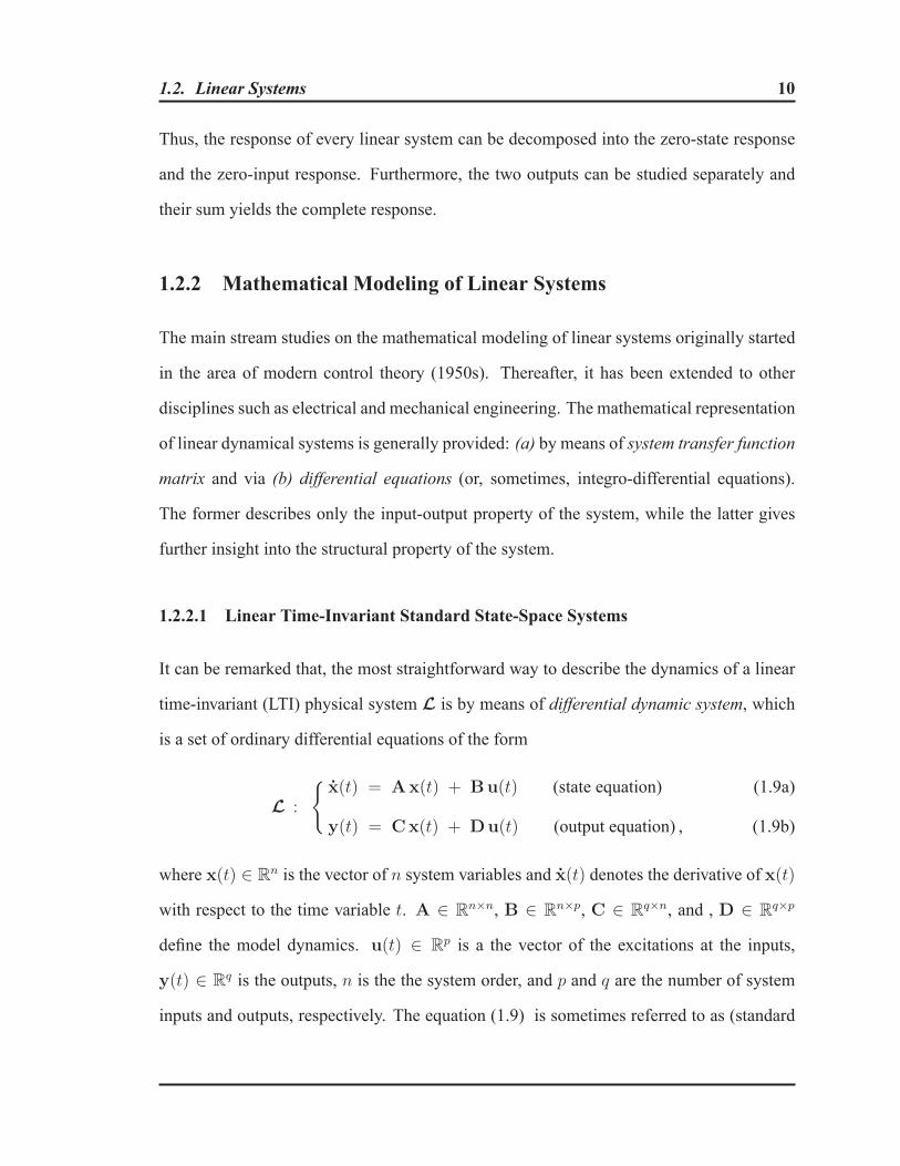
It can be remarked that, the most straightforward way to describe the dynamics of a linear
time-invariant (LTI) physical system L is by means of differential dynamic system, which
is a set of ordinary differential equations of the form
L :
{x(t) = Ax(t) + Bu(t) (state equation) (1.9a)
y(t) = Cx(t) + Du(t) (output equation) , (1.9b)
where x(t) ∈ Rn is the vector of n system variables and x(t) denotes the derivative of x(t)
with respect to the time variable t. A ∈ Rn×n, B ∈ R
n×p, C ∈ Rq×n, and , D ∈ R
q×p
define the model dynamics. u(t) ∈ Rp is a the vector of the excitations at the inputs,
y(t) ∈ Rq is the outputs, n is the the system order, and p and q are the number of system
inputs and outputs, respectively. The equation (1.9) is sometimes referred to as (standard

1.2. Linear Systems 11
or normal) state-space realization of the system.
The state variables are the smallest possible subset of system variables (“state vari-
ables” ⊆ x) that can represent the entire state of the system at any given time. In other
word, the state of a system may be considered to be the minimal amount of information
necessary at any time to completely characterize any possible future behavior of the sys-
tem. This leads to a least order realization of the system. Realizations of least order, also
called minimal or irreducible realizations, are of interest since they realize a system, using
the least number of dynamical elements (minimum number of elements with memory).
1.2.2.2 Solution of Linear Systems
Theorem 1.1. The solution of state equation (1.9a) for prescribed x(t0) = x0 and u(τ),
τ ≥ t0, is unique and is given by
x(t) = eA(t−t0)x0 +
∫ t
t0
eA(t−τ)Bu(τ) dτ . (1.10)
In particular, the solution of the homogeneous equation
x(t) = Ax(t) (1.11)
is
x(t) = eA(t−t0)x0 . (1.12)
For a complete account of the proof, reader is encouraged to directly consult a text in
Ordinary Differential Equation (ODE) e.g. [6–9] or an introductory text in linear system
theory e.g. [4, 5] or a reference for linear circuit theory e.g. [10].

1.2. Linear Systems 12
1.2.2.3 Linear Time-Invariant Descriptor Systems
Discussion of descriptor systems originated in 1977 with the fundamental paper [11].
Since then, the modeling of dynamical systems by descriptor systems (equivalently called
singular systems, or semi-state systems, or differential-algebraic systems, or generalized
state-space systems) have attracted much attention due to the comprehensive applications
in many fields such as electrical engineering [12, 13]. The form of linear Differential-
Algebraic Equation (DAE) so called LTI descriptor model is represented by [14]
L :
{E x(t) = Ax(t) + Bu(t) , with x(t0) = x0 , (1.13a)
y(t) = Cx(t) + Du(t), (1.13b)
where E ∈ Rn×n is generally a singular matrix (i.e. rank(E) = n0 ≤ n). This is a general
state-space equations, often expected in the formulation for circuit simulation.
If there are well-identified input and output variables but little or no interest in the
behavior of the internal variables of the system, a convenient description is provided by
the system impulse response h(t) or its Laplace transform. This is called system transfer
functionmatrix, which is (more or less) the frequency domain equivalent of the time domain
input-output relation [15]. Assuming zero initial conditions, the transfer function matrix
H(s) : C → Cp×p of (1.13) is defined as
H(s)Δ=L (h(t)) =
∫ ∞
0
h(t)e−stdt = C (sE−A)−1B+D , s = δ + jω , (1.14)
where p is the number of input/output ports.
Definition 1.1 (Regularity). A linear descriptor system (1.13a), or the matrix pair (E,A),
is called regular if there exists a constant scalar λ ∈ C such that
det (λE−A) �= 0. (1.15)

1.3. Nonlinear Systems 13
It is also equivalently said that, the matrix pencil (sE−A) of matrix pair (E,A) is regular.
The regularity of systems is the condition to make the solution to descriptor systems exist
and unique. In the following chapters, some special features of regular descriptor linear
systems such as state response and stability will be explained.
Finite Eigenvalues
Under the regularity assumption of the matrix pair (E,A), the polynomial
Δ(s) = det (sE−A) (1.16)
is not identically zero (Δ(s) �≡ 0). This polynomial (1.16) is called the characteristic
polynomial of the system (1.13), which is of a certain degree (e.g. degΔ(s) = n1). Hence,
it has n1 (or less) finite roots (si = λi) satisfyingΔ(s) = 0. The finite roots of the system’s
characteristic polynomial are called the system poles or finite eigenvalues of the system, or
the matrix pair (E,A). Thus, the set of finite poles of the system is
λ (E,A) = {λi | λi ∈ C, λ is finite, det (λiE−A) = 0} . (1.17)
the number of finite poles is always not greater than n1 = rank (E) (≤ n) for descriptor
systems. Therefore, λ (E, A) contains at most n1 number of complex numbers [16].
1.3 Nonlinear Systems
Any system that does not satisfy superposition property is nonlinear. It is worth noting
that, there is no unifying characteristic of nonlinear systems, except for not satisfying “ad-
ditivity” and “homogeneity” properties (cf. 1.2). A very general structure for models of
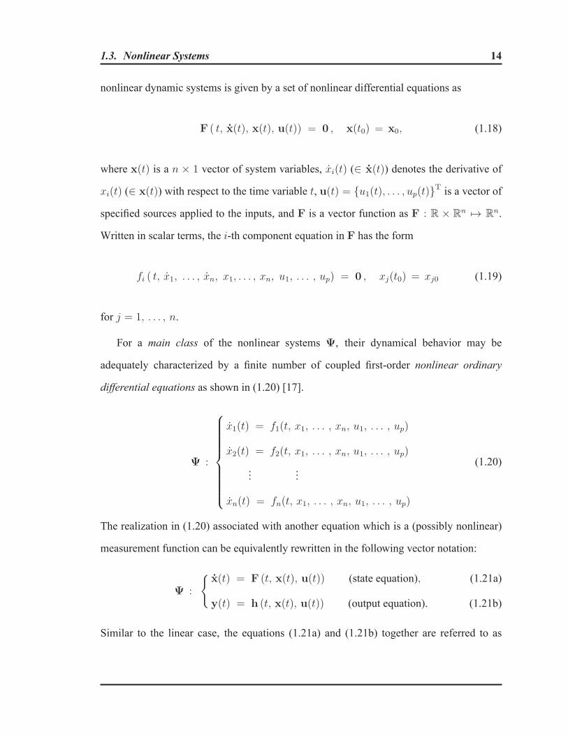
1.3. Nonlinear Systems 14
nonlinear dynamic systems is given by a set of nonlinear differential equations as
F ( t, x(t), x(t), u(t)) = 0 , x(t0) = x0, (1.18)
where x(t) is a n × 1 vector of system variables, xi(t) (∈ x(t)) denotes the derivative of
xi(t) (∈ x(t)) with respect to the time variable t, u(t) = {u1(t), . . . , up(t)}T is a vector ofspecified sources applied to the inputs, and F is a vector function as F : R × R
n �→ Rn.
Written in scalar terms, the i-th component equation in F has the form
fi ( t, x1, . . . , xn, x1, . . . , xn, u1, . . . , up) = 0 , xj(t0) = xj0 (1.19)
for j = 1, . . . , n.
For a main class of the nonlinear systems Ψ, their dynamical behavior may be
adequately characterized by a finite number of coupled first-order nonlinear ordinary
differential equations as shown in (1.20) [17].
Ψ :
⎧⎪⎪⎪⎪⎪⎪⎪⎪⎨⎪⎪⎪⎪⎪⎪⎪⎪⎩
x1(t) = f1(t, x1, . . . , xn, u1, . . . , up)
x2(t) = f2(t, x1, . . . , xn, u1, . . . , up)
......
xn(t) = fn(t, x1, . . . , xn, u1, . . . , up)
(1.20)
The realization in (1.20) associated with another equation which is a (possibly nonlinear)
measurement function can be equivalently rewritten in the following vector notation:
Ψ :
{x(t) = F (t, x(t), u(t)) (state equation), (1.21a)
y(t) = h (t, x(t), u(t)) (output equation). (1.21b)
Similar to the linear case, the equations (1.21a) and (1.21b) together are referred to as

1.3. Nonlinear Systems 15
the (standard) state-space model, or simply the state model. Also, the smallest possible
memory that the dynamical system needs from its past to predict the entire state of the
system at any given future time is called state variables {xi(t) | xi ∈ x(t)}.
One may rightfully question the applicability of (1.21) for all possible cases of nonlinear
physical systems. In the late seventies (1978) [18], it became clear that nonlinear descriptor
systems (1.18), rather than standard Ordinary-Differential Equations (ODE) (1.21), are
more suitable for the modeling of the nonlinear dynamic systems in many applications
such as electrical networks (cf. Sec. 1.4).
1.3.1 Solutions of Nonlinear Systems
There are powerful analysis techniques for linear systems, founded on the basis of the
superposition principle (cf. Sec. 1.2). As we move from linear to nonlinear systems, we
are faced with a more difficult situation. The superposition principle does not hold any
longer and the analysis involves mathematical tools that are more advanced in concept and
involved in detail.
This will be more clear by considering the following facts.
(a) An important property of a linear system is that, when it is excited by a sinusoidal sig-
nal, the steady-state response will be sinusoidal with the same frequency as the input.
Also, the amplitude and phase of the response are functions of the input frequency. In
contrast, when a nonlinear system is excited by a sinusoidal signal, the steady-state
response generally contains higher harmonics (multiples of the input frequencies).
In some cases, the steady-state response also contains subharmonic frequencies.
(b) For nonlinear systems, the complete response can be very different from the sum of
the zero-input response and zero-state response. Therefore, we cannot separate the

1.4. Mathematical Modeling of Electrical Networks 16
zero-input and zero-state responses when studying nonlinear systems.
(c) It is stated in Theorem-1.1 that, any linear system has a unique solution through each
point in the state space for 0 ≤ t ≤ ∞. However, it is only under certain conditionsthat, the nonlinear system has a unique solution at each point in the state space. For
a linear system, the response settles down to a unique solution after the transient dies
out. Nonlinear systems, on the other hand, can exhibit many qualitatively different
coexisting solutions depending on the initial state [19]. In extreme cases, a nonlinear
system can show chaotic behavior.
1.3.2 Linear versus Nonlinear
Nonlinear systems differ from linear systems in several fundamental ways. In Table 1.1
a summary of their general properties and characteristics are compared. More details are
provided in Appendix A.
1.4 Mathematical Modeling of Electrical Networks
Being an inseparable part of the modern era, studying the dynamical behavior and the meth-
ods of mathematical modeling of electrical/electronic networks has moved to the center of
attention in the past few decades. Ever increasing size, complexity and compactness of
electrical designs has been enhancing the importance of such efforts to create accurate
yet efficient system equations. This has been done with the main intention of inclusion of
modern complex products in simulators (and virtual design environments) to ensure more
“realistic” and “efficient” simulations.
(a) Realistic simulations imply that the errors of the virtual models should be small,

1.4. Mathematical Modeling of Electrical Networks 17
Table 1.1: Summary: general properties of linear and nonlinear systemsLinear Systems Nonlinear Systems
x = Ax x = F (x)
Equilibrium Points: Unique Multiple
A point where the system canstay forever without moving.
If A ∈ Rn×n has rank n (full
rank), then xequi = 0; other-wise, the solution lies in the nullspace ofA.
F (xequi) = 0, n coupled non-linear equations in n unknowns;the number of possible solutionsmay vary from 0 to +∞.
Escape Time: x → +∞, as t → +∞ x → +∞, in t ≤ +∞The state of an unstable system: goes to infinity as time ap-
proaches infinity!can go to infinity in finite time!
Stability: The equilibrium point is stable ifall eigenvalues of A have nega-tive real part, regardless of InitialConditions (IC).
Stability about an equilibriumpoint:• Dependent on initial condition• Local vs. Global stability im-portant• Possibility of limit cycles
Oscillation vs. Limit Cycles: Oscillation Limit Cycles
• Needs conjugate poles onimaginary axis• Almost impossible to maintain• Amplitude depends on IC
• A unique, self-excited oscil-lation with fixed amplitude andfrequency• A closed trajectory in the statespace• Independent of IC
Forced Response x = Ax + Bu(t) x = F (x + u(t))
• The principle of superpositionholds.• I/O stability −→ bounded-input, bounded-output• Sinusoidal input −→ sinu-soidal output of same frequency
• The principle of superpositiondoes not hold in general.• The I/O ratio is not unique ingeneral, may also not be single-valued.
Steady-State Behavior Unique Non-unique / Multi-stability
The asymptotic response, whent −→ +∞
The response settles down to aunique solution, independent ofIC.
Can have many different coex-isting solutions depending on IC.
ChaosComplicated steady-state behav-ior, may exhibit randomness de-spite the deterministic nature ofthe system.
The above comparison is based on [20], with enhancements and modifications.

1.5. Overview of Formulation of Circuit Dynamics 18
which requires that, the important physical characteristic of the product must be taken
into account in the mathematical model.
(b) Efficient simulations (maybe paradoxically) imply that it is not necessary to include
all minute detail of a physical design in the simulator.
The latter opens the door to a trend in the area of computational science and engineering as
“model order reduction” that is the main subject in this thesis and its thorough explanation
will be forthcoming. The former explains the importance of the systematic formulation of
the dynamic equations for electrical networks.
The next section presents an overview of the mathematical modeling of electrical net-
works as dynamical systems.
1.5 Overview of Formulation of Circuit Dynamics
Electrical networks (e.g. RLC circuits) are examples of dynamical systems, whose state-
space dynamics for time t ≥ 0, can accurately be captured by a set of first-order coupled
differential equations [21–23]. Since the early sixties, it is known that, descriptive equa-
tions of electrical circuits belong to the class of differential equations on differentiable
manifolds e.g. see [23–26]. This result is related to the celebrated paper of Moser and
Brayton [27] in 1964 where their equations for the description of (reciprocal and) nonlin-
ear circuits are written in coordinates. It lasted another few years until the equations of
Moser and Brayton were reformulated by Smale [22] by means of the framework of mod-
ern differential geometry. Further work was done by Matsomoto [28], Ishiraku [29] and
later by others (e.g.) [30, 31] to refine this approach for describing electrical networks.

1.5. Overview of Formulation of Circuit Dynamics 19
The differential-equation approach to the identification of electrical circuits immedi-
ately led to the necessity of the numerical determination of the transient response, an ex-
tremely important area often more limited by the "stiffness" phenomenon [32, 33]. In the
late sixties, “the time-constant problem” was an infamous source of frustration for users
of computer programs for the analysis of circuits. This obstacle to construct an efficient
and general purpose circuit simulator was solved mainly by contributions of Gear [34] and
Sandberg and Shichman [35]. It was emphasized by Gear (1968) that circuit equations
should be considered as Differential-Algebraic Equations (DAE) (cf. Sec. 1.2.2.3). It was
not until a decade later, when Linda Petzold - a former Ph.D. student of Gear - found out
in 1982 that “DAEs are not ODEs” [36]. She showed that only some of the differential-
algebraic systems can be solved using numerical methods which are commonly used for
solving stiff systems of ordinary differential equations. She also indicated the causes of the
associated difficulties and presented solutions mostly for linear cases.
The DAEs systems to represent electrical networks are directly obtained using the mod-
ified nodal analysis (MNA) matrix formulation [37–39], which will be reviewed in the
following sections.
1.5.1 MNA Formulation of Linear Circuits
In the case that, all the components in the circuit are linear and Kirchoff’s laws also hold,
the circuit is considered as a linear network. Time-domain realization for multi-input and
multi-output (MIMO) dynamical linear circuits (Ψ) in the descriptor form resulting from
MNA matrix formulation [37–39] is represented as:
Ψ :
⎧⎨⎩Cd
dtx(t) + Gx(t) = Bu(t) (1.22a)
y(t) = Lx(t) , (1.22b)

1.5. Overview of Formulation of Circuit Dynamics 20
whereC andG ∈ Rn×n are susceptance and conductance matrices, respectively, x(t) ∈ R
n
denotes the vector of MNA variables (the nodal voltages and some branch currents) [38] of
the circuit. Also, B ∈ Rn×p and L ∈ R
q×n are the input and output matrices, associated
with p inputs and q outputs, respectively.
1.5.2 MNA Formulation of Nonlinear Circuits
The DAE representation for circuits that include non-linearity is generally obtained by
intuitively adding a vector of nonlinear functions representing the nonlinear elements to
(1.22) based on the principals of nodal analysis. It can be rightfully questioned that, how
the result of MNA formulation is related to the general class of nonlinear dynamic systems.
In other words, how much of the generality is scarified by adapting the general formulation
(e.g.) in (1.18). To illuminate this, we cautiously move in a reverse direction. We start from
the general form in (1.18) and by considering the nature of circuits’ topology we attempt
to modify it.
1.5.2.1 A Reverse Approach
The differential-algebraic equations that generally characterize any possible nonlinear sys-
tems (including electrical networks) is shown in (1.18), as repeated here
F (t,x(t), x(t),u(t)) = 0, with x(0) = x0 . (1.23)
Finding a solution for (1.23) in its most general form can be prohibitively complex and
hence, not always possible.
Without loss of generality, nonlinear circuits can be characterized as a system of the

1.5. Overview of Formulation of Circuit Dynamics 21
first order coupled differential equations in the following form:
Σ :
⎧⎨⎩d
dtg (x(t)) = F (x(t) , u(t)) (state equation), (1.24a)
y(t) = h (x , u) (output / measurement equation) , (1.24b)
where x(t) ∈ Rn, u(t) ∈ R
p, y(t) ∈ Rq, g (x(t)), F (x(t) , u(t)) ∈ R
n and h (x , u) ∈R
q.
A complex design consists of sub-circuits that are connected together. These sub-
circuits interact with the surrounding sub-networks through its external nodes as shown
in Fig. 1.2. Taking the state variable approach to MIMO nonlinear electrical networks,
Figure 1.2: Illustration of a subcircuit that accepting p-inputs and interacting with othermodule trough its q-outputs.
there are several established methods, namely sparse-tableau and modified nodal analysis
(MNA) formulation [37–39] to characterize circuits.

1.5. Overview of Formulation of Circuit Dynamics 22
1.5.2.2 MNA Formulation
The electrical networks, as an important class of nonlinear system, can also be well char-
acterized using a system of first order, differential-algebraic equation system as shown in
1.24. The general form of the nonlinear -equations in 1.24 can be adapted to the major
class of the nonlinear dynamical circuits by considering the following remarks:
Remark 1.1. Being expressed in the "normal" DAE form, the nonlinearity is focused on the
state variables F (x(t)). Hence, the state-space equation in (1.24a) will be
Σ :d
dtg (x(t)) = F (x(t)) + P (x(t),u(t)) (state equation) . (1.25)
Remark 1.2. In an electrical network (e.g.: in Fig. (1.2)), the so-called input terminals are
the nodes of the circuit interfacing with the input sources. Hence, the (input) sources are
directly connected to the selected (interface) nodes of the circuit. In the nodal analysis,
the currents from the sources are added to (or subtracted from) the KCL equation for cor-
responding nodes. For the case of voltage sources, the node voltage is directly decided
(equated) by the voltage of the source. Accordingly, it can be generalized that the effect of
the sources is "linearly injected" [40,41] to the system at the associated nodes. To distribute
the effect of the sources, a selection matrix B can be directly applied to the source vector
u(t) to decide the sources connected to each nodes. Under this mild practical assumption,
the system equations for electrical networks fall in affine form in which (1) the source term
is linearly combined with the rest of the formulation and (2) nonlinearities include only in
the constitutive relations for the nonlinear elements as:
Σ :d
dtg (x(t)) = F (x(t)) + Bu(t) (state equation) . (1.26)
Remark 1.3. Even if in a special case, a nonlinear dependence on the input u(t) is assumed

1.5. Overview of Formulation of Circuit Dynamics 23
as B P (v(t)), the nonlinear dependence on input can often be bypassed by treating the
whole term P (v(t)) as input [42]. Thus, the network equations fall in the form shown in
(1.26).
Remark 1.4. The MNA formulation generally leads to certain form for the vector function
F(x) that commonly occurs as F(x) = −Gx(t) + F(x) , where G ∈ Rn×n is
conductance matrix and F(x) ∈ Rn is the vector of nonlinear functions, including all the
nonlinearities in the circuit. Hence, the system equation in (1.26) falls in the following
form
Σ :d
dtg (x(t)) = G(x) + F (x(t)) + Bu(t) (state equation) . (1.27)
Remark 1.5. Based on a similar approach for inputs, outlined in Remark-1.2 the outputs
in MNA formulation y(t) are simply selections (generally not many) of the the voltages
and currents in x(t). This selection can be performed by applying a properly decided
selection matrix L in the output equation. Let us stress that in the MNA formulation the
output signals are not explicitly dependent on the inputs u(t). Hence, the output equation
commonly occurs in the form shown in (1.28b).
In summary, the electrical systems whose dynamics are formulated based on the MNA
approach at time t can be generally described by the nonlinear, first order, differential-
algebraic equation system. The equations encountered often in the practical situations is of
the form:
Σ :
⎧⎨⎩d
dtg (x(t)) = −Gx(t) + F (x(t)) + Bu(t), x(0) = x0, (1.28a)
y(t) = Lx (t) , (1.28b)
where x(t) ∈ Rn denotes the vector of circuit variables in time t. The vector-valued
functions g , F ∈ Rn respectively represent the NL susceptances of (e.g.) nonlinear
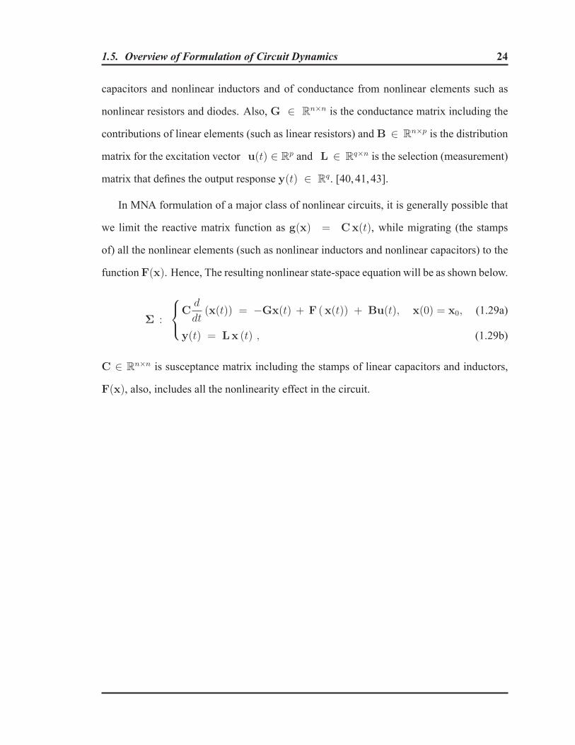
1.5. Overview of Formulation of Circuit Dynamics 24
capacitors and nonlinear inductors and of conductance from nonlinear elements such as
nonlinear resistors and diodes. Also, G ∈ Rn×n is the conductance matrix including the
contributions of linear elements (such as linear resistors) and B ∈ Rn×p is the distribution
matrix for the excitation vector u(t) ∈ Rp and L ∈ R
q×n is the selection (measurement)
matrix that defines the output response y(t) ∈ Rq. [40, 41, 43].
In MNA formulation of a major class of nonlinear circuits, it is generally possible that
we limit the reactive matrix function as g(x) = Cx(t), while migrating (the stamps
of) all the nonlinear elements (such as nonlinear inductors and nonlinear capacitors) to the
functionF(x). Hence, The resulting nonlinear state-space equation will be as shown below.
Σ :
⎧⎨⎩Cd
dt(x(t)) = −Gx(t) + F (x(t)) + Bu(t), x(0) = x0, (1.29a)
y(t) = Lx (t) , (1.29b)
C ∈ Rn×n is susceptance matrix including the stamps of linear capacitors and inductors,
F(x), also, includes all the nonlinearity effect in the circuit.
Chapter 2
Model Order Reduction - Basic Concepts
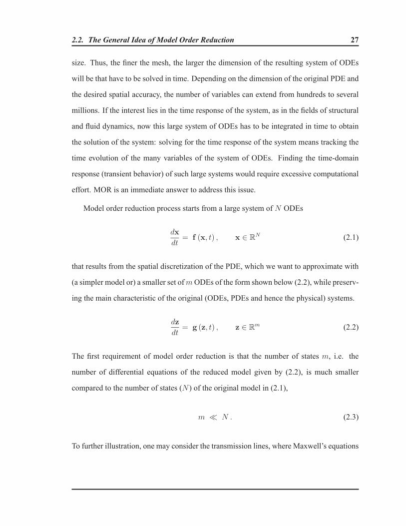
One may find a variety of interpretations for the topic of model order reduction in different
disciplines. The common theme in all of them is that, given a large-scale dynamical system
(linear or nonlinear) with predefined input and output terminals, a small-scale system is
found that approximates the behavior of the original system at its terminals. To achieve this,
the concepts and techniques of mathematical approximation for large differential-equation
systems come into the picture. Hence, the concepts of MOR has generally been associated
with the terms such as “dimensionality reduction”, “reduced-bases approximation”, “high
energy dynamic modes”, “balancing the gramians” and “state truncation”. The concept
itself and even almost all the techniques have been originally introduced in mathematics,
mainly in the context of differential equations. Due to the feasibility of the idea, later it
has been carried over to the control area and then to the fields such as civil engineering,
aerospace engineering, earthquake engineering, mechanical andMicro-Electro-Mechanical
Systems (MEMS), and VLSI circuits design which is the main subject of focus in this
thesis.
This chapter provides an introduction and explains the fundamental concepts relevant to the
subject of this thesis, in which we consider approximations of continuous-time dynamical
systems.
25

2.1. Motivation 26
2.1 Motivation
The problem of model order reduction of linear and nonlinear dynamical systems has been
widely studied in the last two decades and is still considered an active topic, attracting
much attention. Due to the ever-enhancing capability of methods and computers to ac-
curately (and thus complexly) model real-world systems, simulation or, more generally,
computational science has been proven as a reliable method for identifying, analyzing and
predicting the behavior of systems. This is to such a degree that, simulation has become
an important part of today’s technological world, and it is now generally accepted as the
third discipline, besides the classical disciplines of theory and experiment (analytical and
observational forms).
Computer simulations are now utilized in almost every physical, chemical and other
processes. Computer Aided design and virtual environments have been set up for a variety
of problems to ease the work of designers and engineers. In this way, new products can be
designed faster, more reliably, and without having to make costly prototypes [44]. In order
to speed up the computation time it is a good idea to simplify the model, either in size or in
complexity. Reducing the order of a model involves reducing the size of the mathematical
model, but at the same time to preserve its essential features.
2.2 The General Idea of Model Order Reduction
A major class of physical systems and phenomena can be mathematically modeled [2,
45, 46] with a set of Partial Differential Equations (PDE), which adequately describes the
physical behavior of the system under consideration. The spatial discretization of the PDE
yields a system of ordinary differential equations (ODE), which in turn approximates the
original PDE model. The dimension of this ODE system is governed by the spatial mesh
2.2. The General Idea of Model Order Reduction 27
size. Thus, the finer the mesh, the larger the dimension of the resulting system of ODEs
will be that have to be solved in time. Depending on the dimension of the original PDE and
the desired spatial accuracy, the number of variables can extend from hundreds to several
millions. If the interest lies in the time response of the system, as in the fields of structural
and fluid dynamics, now this large system of ODEs has to be integrated in time to obtain
the solution of the system: solving for the time response of the system means tracking the
time evolution of the many variables of the system of ODEs. Finding the time-domain
response (transient behavior) of such large systems would require excessive computational
effort. MOR is an immediate answer to address this issue.
Model order reduction process starts from a large system of N ODEs
dx
dt= f (x, t) , x ∈ R
N (2.1)
that results from the spatial discretization of the PDE, which we want to approximate with
(a simpler model or) a smaller set ofmODEs of the form shown below (2.2), while preserv-
ing the main characteristic of the original (ODEs, PDEs and hence the physical) systems.
dz
dt= g (z, t) , z ∈ R
m (2.2)
The first requirement of model order reduction is that the number of states m, i.e. the
number of differential equations of the reduced model given by (2.2), is much smaller
compared to the number of states (N ) of the original model in (2.1),
m � N . (2.3)
To further illustration, one may consider the transmission lines, where Maxwell’s equations

2.3. Model Accuracy Measures 28
(the equations describing electromagnetic fields) are applied to the geometry. The trans-
mission line equations (Telegrapher’s equations) [47] can be derived by discretizing the
line into infinitesimal section of length (Δx) and assuming uniform per unit length (p.u.l.)
parameters of resistance, inductance, conductance, and capacitance. The segments of the
line are decided to be electrically small (much smaller than a wavelength at the excita-
tion frequency), to the aim that, lumped-circuit approximation of the exact per-unit-length
distributed-parameter model can be adequately used. As a result, a cascade structure of
multiple lumped filter sections (and Kirchhoff’s laws) is used to replace Maxwell’s equa-
tions in analyzing transmission lines. The ODEs formulation for such large circuits, having
a few thousands variables for each interconnect, can be prohibitively large, even with a
moderate accuracy expectation. Chapter 5 explains, how model order reduction can be
utilized to address this issue.
The idea of MOR has been proved as an useful tool to obtain efficiency in simulations
while ensuring desired accuracy. Its applicability to real life problems has made it a poplar
tool in many branches of science and engineering. Fig. 2.1 pictorially explains this process.
2.3 Model Accuracy Measures
Attainable accuracy from the resulting reduced macromodel is an important concern in
the reduction process. To decide, how well a reduced system approximates the original
system, we require a measure to quantify the accuracy. The straightforward way is to
define the error (time-domain) signal ζ(t) as the deviation between two responses, from
the model and from the original system as illustrated in Fig. 2.2. The difference between
outputs should be measured at the same n time instances and for the same input signal
u(t). For the case of linear systems such deviation can also be judged comparing the

2.3. Model Accuracy Measures 29
Physical System
PDE
Large system of
ODE
Reduced system of
ODE
Mathematical
Modeling
Discretization
Model order
reduction
Approximated
Solution
Simulation
Figure 2.1: Model order reduction.
Original System
Reduced Model
+
_
u(t)
Figure 2.2: Measuring error of approximation.

2.3. Model Accuracy Measures 30
frequency response of the original system and the one from the reduced transfer function
at the n frequency points throughout the frequency spectrum of interest. The results for
“single-input and single-output” (SISO) systems will be a vector and for “multi-input and
multi-output” (MIMO) cases it is a matrix containing the instantaneous errors at different
“ports”.
The error space (the space, where error resides) is considered as metric space (defini-
tion B.3) endowed with different norms that can be properly used to characterize the error
(Sec. B.1.2). Table 2.1 presents a summary of the commonly used measures to quantify the
error in the context of (linear / nonlinear) MOR.
Table 2.1: Measuring reduction accuracy in time domainName Definition of E
mean squared error ‖ζ‖2en , where ‖·‖e is Euclidean norm
normalized mean squared error ‖ζ‖2evar(y)
,
where “var” denotes the variance ∗ of data set
root mean squared error ‖ζ‖e√n
normalized root mean squared error ‖ζ‖e√var(y)
mean absolute error ‖ζ‖1n
mean absolute relative error
∥∥∥∥ζy∥∥∥∥1
n
*- For a data set y = {yi} including N data points, variance is computed as
var(y) �1
N
N∑i=1
(yi − y)2, where y is the data mean y �1
N
N∑i=1
yi.
It is to be noted that, depending on the application, other accuracy measures can also
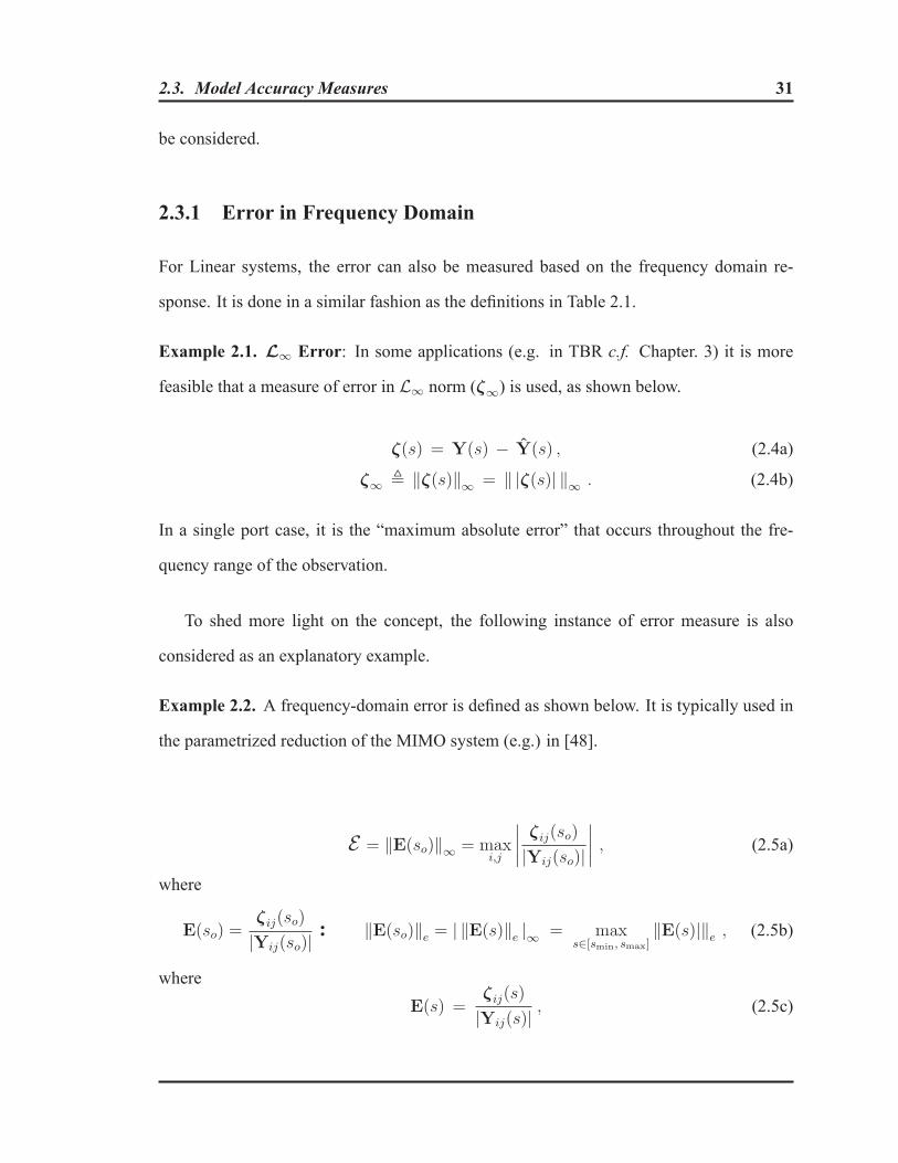
2.3. Model Accuracy Measures 31
be considered.
2.3.1 Error in Frequency Domain
For Linear systems, the error can also be measured based on the frequency domain re-
sponse. It is done in a similar fashion as the definitions in Table 2.1.
Example 2.1. L∞ Error: In some applications (e.g. in TBR c.f. Chapter. 3) it is more
feasible that a measure of error in L∞ norm (ζ∞) is used, as shown below.
ζ(s) = Y(s) − Y(s) , (2.4a)
ζ∞ � ‖ζ(s)‖∞ = ‖ |ζ(s)| ‖∞ . (2.4b)
In a single port case, it is the “maximum absolute error” that occurs throughout the fre-
quency range of the observation.
To shed more light on the concept, the following instance of error measure is also
considered as an explanatory example.
Example 2.2. A frequency-domain error is defined as shown below. It is typically used in
the parametrized reduction of the MIMO system (e.g.) in [48].
E = ‖E(so)‖∞ = maxi,j
∣∣∣∣ ζij(so)
|Yij(so)|∣∣∣∣ , (2.5a)
where
E(so) =ζij(so)
|Yij(so)| : ‖E(so)‖e = | ‖E(s)‖e |∞ = maxs∈[smin, smax]
‖E(s)|‖e , (2.5b)
whereE(s) =
ζij(s)
|Yij(s)| , (2.5c)

2.4. Model Complexity Measures 32
and whereζij(s) = Yij(s) − Yij(s) . (2.5d)
The error in (2.5) can be determined according to the following explanations.
• At each frequency point, every entry of the absolute error matrix from (2.5d) is nor-
malized (scaled) by the magnitude of the corresponding entry in the original response
matrix, as shown in (2.5c).
• E(so) in (2.5b) is the normalized error matrix evaluated at the frequency point so
such that, it has the maximum euclidean norm in the frequency spectrum of interest
s ∈ [smin, smax].
• The error E in (2.5a) is defined as the magnitude of the entry in E(so) matrix whichhas the largest magnitude when compared to the other entries.
This measure is adequate if one wants to preserve very small entries of the transfer function,
or in cases where at certain frequencies the transfer function is infinitely large [48].
2.4 Model Complexity Measures
As we already explained, the main intention of applying model order reduction is to reduce
costs of simulation of such systems. Hence, in a general sense, the (CPU) time associated
with simulating the model alone or as a sub-system in a hierarchy of a system can be used
as a practical measure for the complexity of the model. As models become more complex,
simulation cost also rises.
It is to be noted that, while the original system (specifically in circuit theory) is highly
sparse, any attempt of reduction can impair the sparsity to a certain degree. For systems

2.5. Main Requirements for Model Reduction Algorithms 33
with many I/O terminals, this fact may preclude any advantage expected from MOR (c.f.
Chapter 5).
2.5 Main Requirements for Model Reduction Algorithms
A number of requirements should necessarily be satisfied, when extracting the macromodel
from a detailed physical description of the original system. The most important ones that
ensure feasibility of the resulting models may be summarized as follows
• Accuracy: The reduction technique should lead to an adequately accurate model for
the original system. The reduced model should closely follow the terminal behavior
of the original system.
• Compactness: It should significantly reduce the number of variables or states, as
compared to the original model.
• System properties preservation: For many types of problems, it is desirable that
the reduced models conserve the main physical properties of the original system, i.e.
passivity and stability. Due to the importance of such characteristics, further details
are discussed in Sections 2.6 and 3.1.
• Computationally efficient: The MOR algorithm should extract a model which
is relatively inexpensive to simulate and store it in the computer’s memory. The
computational cost for simulating the resulting model should be much lower than the
cost for the original model.
• Inexpensive algorithm: The model reduction algorithm should be relatively inex-
pensive to apply and it is preferable to be automated. In other words, the extraction

2.6. Essential Characteristic of Physical Systems 34
process needs to be practically repeatable in any phase of design, optimization or
verification directly by the designers with a reasonable cost.
The resulting reduced model should accurately mimic the dynamics of the original subsys-
tem in operating regimes which are different from the ones used to construct the model.
This assures the accuracy of the results when the submodel is embedded in the hierar-
chy of a design and undergoes a higher level system level simulation. This property is
referred to as Transportability [49] in the literature of nonlinear behavioral macromodel-
ing [19, 49–54].
2.6 Essential Characteristic of Physical Systems
Among the essential characteristic that should be passed on to the successor representative
of physical systems, stability and passivity are prominent. This section reviews the basic
concepts and definitions in the most general form. Due to its direct relevance to our work,
later in this report, we will study the detail of stability and passivity for linear and nonlinear
systems.
2.6.1 Stability of Dynamical Systems
General stability concepts and theory play a central role in studying dynamical systems and
have been extensively studied in the literature of system theory [4,5,17,48,55–58]. For an
arbitrary dynamical system, stability is studied in the frame of two major notions:
(a) Internal stability: The internal stability considers the trajectory (response curve) of
an autonomous system
x(t) = F(x(t)), (2.6)

2.6. Essential Characteristic of Physical Systems 35
that is a time invariant system without any input. The response of autonomous sys-
tems (2.6) is only due to the nonzero initial state X0, that is also called, zero-input
response. It is referred to as internal because such stability is decided based on the
internal dynamics of the system without any outside intervention.
(b) External stability: The external stability (so-called, Input-Output stability) is con-
nected with how much the system amplifies the input signals to provide the output.
The following stabilities are well-known in literature and have been extensively studied
[17][ch.:4,5,7,8], [4, 5, 57, 58].
2.6.2 Internal Stability
For an autonomous system in (2.6), internal stability can be studied as global or local
stability of “equilibrium states”. An equilibrium point is a state that the autonomous system
can maintain for an infinite time.
2.6.2.1 Local Stability of Equilibrium Points
Definition 2.1 (Lyapunov stability). An equilibrium state of (2.6) xeq is called Lyapunov
stable (or simply stable), if ∀ ε > 0, ∃ δ = δ(ε) > 0, such that
‖x(t0)− xeq‖ < δ =⇒ ‖x(t)− xeq‖ < ε , ∀ t > t0 (2.7)
otherwise it is not stable.
This states that, an equilibrium point is called (Lyapunov) stable if all solutions starting at
nearby points stay nearby and remains bounded as t → ∞ (without necessarily going to
zero); otherwise, it is unstable.

2.6. Essential Characteristic of Physical Systems 36
Definition 2.2 (Asymptotic stability). An equilibrium state of (2.6) xeq is asymptotically
stable if it is Lyapunov stable and δ can be chosen such that
‖x(t0) − xeq‖ < δ =⇒ limt→∞
x(t) = xeq . (2.8)
It is said that, an equilibrium point is asymptotically stable if all solutions starting at nearby
points not only stay nearby (i.e. Lyapunov stable), but also tend to the equilibrium point x0
as time approaches infinity. Loss-less (conservative) systems, such as pure LC circuits, are
examples of (Lyapunov) stable but are not asymptotically stable systems.
In 1892, Lyapunov showed that certain other functions (hence the name Lyapanov func-
tions) could be used instead of energy to determine stability of an equilibrium point as
shown in the following Lyapunov theorem. For convenience, we state the theorem for the
case when the equilibrium point is at the origin of Rn; that is, xeq = 0. There is no loss
of generality in doing so because any equilibrium point can be shifted to the origin via a
change of variables.
Theorem 2.1 (Lyapunov’s stability theorem [17, 59] ). Let xeq = 0 be an equilibrium
point for x = F(x) andD ⊂ Rn be a domain containing xeq = 0 (origin). LetV : D �→
R be a contentiously differentiable function such that
V (0) = 0 and V (x) > 0 inD − {0} . (2.9)
If
V (x) ≤ 0, inD (2.10)
then, x = 0 is stable. Moreover, if
V (x) < 0 in D − {0} (2.11)

2.6. Essential Characteristic of Physical Systems 37
then x = 0 is asymptotically stable.
In Theorem 2.1, V (x) denotes the derivative of V (x) along the trajectories of
x = F(x) = [f1(x) . . . fi(x) . . . fn(x)]T , (2.12)
given by
V (x) =n∑
i=1
∂V
∂xi
xi =n∑
i=1
∂V
∂xi
fix =
[∂V
∂x1
,∂V
∂x2
, . . . ,∂V
∂xn
]⎡⎢⎢⎢⎢⎢⎢⎢⎢⎢⎢⎢⎢⎣
f1(x)
f2(x)
...
fn(x)
⎤⎥⎥⎥⎥⎥⎥⎥⎥⎥⎥⎥⎥⎦=
∂V
∂xF(x) . (2.13)
It is to be noted that, Lyapunov stability theorem’s conditions are only sufficient. They do
not say whether the given conditions are also necessary. Hence, failure to satisfy the con-
ditions for stability or asymptotic stability does not mean that the equilibrium is not stable
or asymptotically stable. It only means that such a stability property cannot be established
by using the Lyapunov function shown in Theorem 2.1. Whether the equilibrium point is
stable (asymptotically stable) or not can be determined only by further investigation. For
more details one can consult [17].

2.6. Essential Characteristic of Physical Systems 38
2.6.2.2 Global Stability of Equilibrium Points
Theorem 2.2 (Global asymptotic stability theorem [17] ). Let x = 0 be an equilibrium
point for x = F(x). LetV : Rn �→ R be a contentiously differentiable function such that
V (0) = 0 and V (x) > 0 ∀ x �= 0 (2.14)
‖x‖ → ∞ ⇒ V (x) → ∞ (2.15)
V (x) < 0 ∀ x �= 0 (2.16)
then x = 0 is globally asymptotically stable.
2.6.3 External Stability
An input u(t) is said to be bounded if there exists a constant α such that |u(t)| ≤ α < ∞for −∞ < −T ≤ t < ∞, where T is any arbitrary time point prior to the reference timet = 0. Or, it can be said that a bounded signal does not grow to positive or negative infinity.
We shall say that a causal system is BIBO-stable (bounded input - bounded output stable)
if a bounded input necessarily produces a bounded output |y(t)| < γ for −T ≤ t < ∞.
2.6.4 Passivity of a Dynamical Model
Another important characteristic for the models is passivity. It is said that, reduced model
for a passive original system should preserve passivity. It is important because, stable
but non-passive models may lead to unstable systems when connected to other passive
components. On the other hand, a passive macromodel, when terminated with any arbitrary
passive load, always guarantees the stability of the overall network. Generally speaking, a
model of a circuit is passive if it does not generate energy. This notion ultimately depends

2.7. The Need for MOR for Electrical Circuits 39
on the nature of the input and output signals as shown below.
Definition 2.3 (Passivity [17]). The system y = h(t, u) is
• passive if uTy ≥ 0,
• lossless if uTy = 0,
for all (t, u).
2.7 The Need for MOR for Electrical Circuits
The ever increasing demand for higher data rates, lower power, and multifunction capa-
ble products are necessitating newer generations of complex and denser electronic circuits
and systems. With the rapid increase in signal-speeds and decreasing feature sizes, high-
frequency effects become the dominant factors limiting overall performance of microelec-
tronic systems. The high complexity in design and the necessity of capturing the high-speed
effects lead to extremely large models, to ensure sufficient accuracy in simulations. The
processing cost for simulation of such large models can be prohibitive. It is to be noted that,
the simulation of these models generally needs to be repeated many times during design,
optimization and verification processes. Initial interest in model reduction (MOR) tech-
niques stemmed from efforts to improve the simulation efficiency by reducing the circuit
complexity while producing a good approximation for the input-output behavior of large
structures. Hence, MOR is specifically useful when a compact macromodel is required to
represent the signal behavior at the ports of the circuit block in a higher level simulation.
The order reduction problems (in general) can be categorized as linear MOR and nonlinear
MOR. Reduced-order modeling is well established for linear circuit systems such as elec-
trical interconnect, whereas the available techniques for reduction of nonlinear circuits are
limited in number and the scope of application. The complex nature of nonlinear phenom-
ena makes nonlinear model order reduction a challenging area.

Chapter 3
Model Order Reduction for Linear Dynamical
Systems
The previous chapter (2) presented a general discussion on computational science, and the
need for compact models of phenomena observed in nature and industry. It was remarked
that, the basic motivation for system approximation is the need for simplified models of
dynamical systems, which capture the main features of the original complex models such
as stability. This need arises from limited accuracy, computational power, and storage
capabilities. The main goal of the efforts made in the field of linear model (order) reduction
has been aimed at creating such simplified (but adequately accurate) models that can be
properly incorporated in higher level simulations in place of the original complex models.
This thesis is mainly focused on the application of the MOR techniques on electrical
circuit simulation problems such as the ones arising in the current high-performance VLSI
designs (see [60–62], but also work of others). For this purpose, the current chapter is
dedicated to the subject of compact modeling of general linear time invariant (LTI) systems
such as on-chip interconnects which are modeled as linear RLCM circuits. Due to the
practical importance, providing ingenious solutions to reduce the complexity of resulting
macromodels has been an active area of research within the last three decades. As a result,
40

3.1. Physical Properties of Linear Dynamical Systems 41
a rich body of literature is available covering the linear MOR techniques [44, 63–66] for
compact modeling and analysis of linear circuits. It reviews some fundamental concepts
and techniques of model reduction for linear time invariant (LTI) circuits. Chapters 5 and
6 present numerical examples of the application of Linear MOR on the Linear circuits and
address some associated issues.
3.1 Physical Properties of Linear Dynamical Systems
There are intrinsic properties for the physical linear systems such as causality, stability,
and passivity. To obtain model from a reduction process whose behavior stays faithful to
the original system, conservation of the main physical characteristics of original systems is
necessary. In other words, the compact models should inherit the essential properties from
the original systems, among which the following characteristics are important.
3.1.1 Stability of Linear Systems
Stability is regarded as one of the most important properties of dynamical systems. It deals
with the boundedness properties and the asymptotic behavior (as t → ∞) of the transientsolution of a zero-input state-equation (1.13) with respect to initial condition disturbances.
Hence, it is often crucial [67] that reduced-order models inherit the stability properties of
the original system. Due to its application in circuit analysis, the stability of continuous-
time (LTI) descriptor (DAE) systems(1.13) is explained. The equation (1.13) is repeated
below for ease of reference,
L :
{E x(t) = Ax(t) + Bu(t) , with x(t0) = x0 , (3.1a)
y(t) = Cx(t) + Du(t). (3.1b)

3.1. Physical Properties of Linear Dynamical Systems 42
The standard state-space equations (1.9) can be considered as a special case of descriptor
systems (3.1), where E is invertible (rank(E) = n = dim(A)). Hence, the analogous
results can be obtained for state-space systems.
3.1.1.1 Internal Stability
To study the internal stability of descriptor linear systems, one needs only to consider the
system state-equations 1.9a or 3.1a under zero-input conditions (homogeneous form).
The first stability notion based on the boundedness of solutions of (3.1) is uniform
stability. Because solutions are linear in the initial state (cf. 1.2), it is convenient to express
the bound as a linear function of the initial state.
Definition 3.1 (Uniform Stability [58]). The linear descriptor equations (3.1) is called
uniformly stable if there exists a finite positive constant γ such that for any t0 and x0 the
corresponding solution satisfies
‖x(t)‖ ≤ γ ‖x0‖ , t ≤ t0 . (3.2)
The adjective uniform in the definition refers precisely to the fact that σ must not depend
on the choice of initial time, as illustrated in Fig. 3.1. This figure also depicts the appli-
cability of the concept to a general class of linear systems including time-varying types,
where the system matrices are time dependent, i.e. A(t) and B(t).
For the case of standard state-space systems (1.9), where an state-transition matrix can be
explicitly defined as shown in (3.3) [5], it is natural to begin by characterizing the stability
of the linear state equation (1.9a) in terms of bounds on the transition matrix.
Φ(t, τ) = eA(t−τ), ∀ t, τ (3.3)

3.1. Physical Properties of Linear Dynamical Systems 43
t
Figure 3.1: Illustrates the uniform stability; uniformity implies the σ-bound is independentof t0.
Theorem 3.1. The linear system is uniformly stable if and only if there exist a finite positive
constant γ such that
‖Φ(t, τ)‖ ≤ γ (3.4)
for all t, τ such that t ≥ τ .
The behavior of the state-transient matrix as defined in (3.4), is totally determined by
the eigenvalues of matrix A (poles). In regards to this, from the the boundedness of the
response characterized by uniform stability, the following conclusion is readily discernible.
Theorem 3.2 (Marginal stability [5]). The causal system x = Ax is marginal stable if
and only if all real parts of eigenvalues of A are nonpositive (zero or negative) and those
with zero real parts are simple roots of the minimal polynomial ofA.
Marginal stability requires that, all pure imaginary eigenvalues ofA to be simple and only
occur in 1 × 1 blocks in the Jordan form of A. This ensures that, the state x(t), resulting
from any nonzero initial state, will remain bounded under zero-input conditions.
Next, a stability property for (3.1a) that addresses both boundedness and asymptotic
behavior of solutions is considered. It implies uniform stability, and imposes an additional

3.1. Physical Properties of Linear Dynamical Systems 44
requirement that all solutions approach zero exponentially as t → ∞.
Definition 3.2 (Uniform Exponential Stability [16,58]). System (3.1a) is called uniformly
exponentially stable if there exist finite positive constants α, β, such that for any t0 and x0
the corresponding solution satisfies
‖x(t)‖ ≤ αe−β(t−t0) ‖x0‖ , t ≤ t0 (3.5)
where the scalar β is called the decay rate.
This is illustrated in Fig. 3.2. Similar to Fig.-3.1 this figure also infers the applicability of
the concept to a general class of linear systems including time-varying. Definition 3.5 is
t0
t
Figure 3.2: A decaying-exponential bound independent of t0.
equivalent to limt→+∞
x(t) = 0, so called asymptotically stable.This implies that the state x(t)
resulting from any nonzero initial state x(t0), given enough time, will decay to zero state
under a zero-input condition.
The asymptotic stability can also be examined with regards to the system poles through the
following theorem.

3.1. Physical Properties of Linear Dynamical Systems 45
Theorem 3.3 ( [16,68]). The regular descriptor linear system (3.1) is asymptotically stable
if and only if
λ (E,A) ⊂ C− = {λi | λi ∈ C, det (λiE−A) = 0, �e (λi) < 0} . (3.6)
It is to be noted that, λ (E,A) ⊂ C− stands for the field of finite poles with negative real
parts.
The above facts are strongly desirable to be extended to standard state-space systems
(1.9a), leading to the following conclusion.
Theorem 3.4 (Asymptotic stability [5]). The causal state-space system x = Ax is
asymptotically stable if and only if all the eigenvalues of A have strictly negative real
parts, that is,A is Hurwitz.
The celebrated Lyapunov stability theory is another suitable mean to analyze the stability
of linear systems.
Theorem 3.5 (Lyapunov Stability [4, 5, 63]). The causal system x = Ax is asymptot-
ically stable, i.e. �{λ(A)} < 0 for all eigenvalues of A, if and only if for any given
positive-definite symmetric matrix Q there exists a positive-definite (symmetric) matrix P
that satisfies
AT P + PA = −Q . (3.7)
A Lyapunov equation theory for the stability of descriptor linear systems has also been
established in the descriptor linear systems literature (e.g. [69] and the references therein).
It is referred to as the generalized Lyapunov matrix equations, and falls in the following
form [68,70],

3.1. Physical Properties of Linear Dynamical Systems 46
Theorem 3.6 (Generalized Lyapunov Stability [68] [4,5,63]). A causal descriptor system
(3.1a) is regular and asymptotically stable if and only if for any given positive-definite
symmetric matrixQ there exists a positive-definite (symmetric) matrix P that satisfies
AT PE + ET PA = −ETQE. (3.8)
satisfying
rank(ET PE
)= rank (P) = r . (3.9)
3.1.1.2 External Stability
A causal system is externally stable if a bounded input, u(t) < M1 for −∞ < −T ≤ t <
∞, produces a bounded output y(t) < M2, −T ≤ t < ∞. A necessary and sufficientcondition for bounded-input and bounded-output (BIBO) stability is defined based on its
impulse response h(·) as presented in the following theorem.
Theorem 3.7 (BIBO stability [4, 5, 63]). A SISO system is bounded-input and bounded-
output (BIBO) stable if and only if its impulse response h(t) is absolutely integrable in
[0, ∞), i.e.∞∫0
|h(t)|dt ≤ M < ∞ , (3.10)
for some constant M . In discussing external stability, we shall assume zero initial
conditions.
3.1.2 Passivity of Linear Systems
Roughly speaking, passive systems are systems that do not generate energy internally. In
other words, the energy dissipated in the system is never greater than the energy supplied

3.1. Physical Properties of Linear Dynamical Systems 47
to it.
3.1.2.1 Hybrid Case (Admittance and Impedance)
According to the positive-real lemma, an asymptotically stable network is passive if its
transfer-function matrixH(s) (in admittance or impedance form) is positive real. Strictly
speaking, fulfillment of the conditions in the following theorem implies that the underlying
state-space description is a representation of a passive system [10,71–73].
Theorem 3.8. An impedance/admittance matrixH(s) represents a passive linear system if
and only if
Each element of H(s) is analytic in C+ (∀s : �e(s) > 0) , (3.11a)
H(s) = H(s) (3.11b)
Φ(s) = HH(s) +H(s) ≥ 0; ∀s : �e(s) > 0 ,
where Φ(s) is positive semi-definite.(3.11c)
The second condition (3.11b) ensures that all the coefficients in numerator and denomi-
nator polynomials are real and hence, the associated impulse response is also real. The third
condition (3.11c) is a generalization of the fact that “a passive one-port impedance/admit-
tance must have a positive real part” to the matrix case for multiport systems. A matrix that
fulfills these three conditions is said to be positive real. For the physical systems which are
asymptotically stable, positive-realness can be equivalently investigated by checking one
equation as shown in (3.12),
Φ(s) = H(s) + HT(s) ≥ 0 ∀s : s ∈ C+. (3.12)

3.1. Physical Properties of Linear Dynamical Systems 48
3.1.2.2 Scattering Case (s-parameters)
For a scattering representation, the first and the second condition are still valid. Only, it
should be noted that for scattering representations no poles are allowed on the imaginary
axis [10]; accordingly, condition two must hold for s ∈ C+. Hence, a scattering matrix
transfer function H(s) represents a passive linear system if it fulfills the following condi-
tions [10, 72]
Each element of H(s) is analytic in C+ (∀s : ��(s) ≤ 0) , (3.13a)
H(s) = H(s) , (3.13b)
Φ(s) = I−HH(s)H(s) ≥ 0; ∀s : s ∈ C+
where Φ(s) is positive semi-definite.(3.13c)
A matrix fulfilling these three conditions is said to be bounded real. A matrix is positive
semi-definite when all its spectrum (eigenvalues) are a non-negative values. To investigate
this for (3.13c) we mathematically have
λ(I−HHH
)= 1− λ
(HHH
) ≥ 0 , (3.14)
or equivalently
λ(HHH
) ≤ 1 , (3.15)
which directly implies,
λmax
(HHH
) ≤ 1 . (3.16)
Knowing λi
(HHH
)= σ2
i (H) [74], from (3.16) it is
σ2max (H) ≤ 1 , (3.17)

3.2. Linear Order Reduction Algorithms 49
and hence,
σmax (H) ≤ 1 . (3.18)
Theorem 3.9 (The Courant-Fischer Theorem for Singular Values [75]). Suppose H ∈C
m×n, n ≤ m, has singular values σ1 ≥ σ2 ≥ · · · ≥ σn. Then for k = 1, . . . , n
σk = mindim(S)=n−k+1
maxx∈Sx �=0
‖Ax‖2‖x‖2
= maxdim(S)=k
minx∈Sx �=0
‖Ax‖2‖x‖2
. (3.19)
From the above theorem, it is straightforward to conclude the following
Corollary 3.1. GivenH(s) ∈ Cp×p for any s ∈ C+, it is
σmax(H(s)) = maxx∈C−{0}
‖H(s)x(s)‖2‖x(s)‖2
Δ= ‖H(s)‖2 , ∀s : �e(s) ≥ 0 . (3.20)
Considering (3.20) from corollary 3.1, an alternative form for passivity condition is
obtained as shown in (3.21)
‖H(s)‖2 ≤ 1 . (3.21)
To conclude, it is highlighted that, stability and passivity are the physical properties of the
original system that should be preserved in a model order reduction process. It is important
because, stable but non-passive models may lead to unstable systems when connected to
other passive components. On the other hand, a passive macromodel, when terminated with
any arbitrary passive load, always guarantees the stability of the overall network.
3.2 Linear Order Reduction Algorithms
There are a number of methods that have been developed for model order reduction of
large electrical networks. Among those, the followings are widely used and known to be

3.3. Polynomial Approximations of Transfer Functions 50
successful in accomplishing a compact model representation.
A. Polynomial approximations of the transfer functions:
i) Explicit moment matching techniques and asymptotic waveform evaluation(AWE)
B. Projection based techniques:
i) Krylov-subspace methodsii) SVD based methods
• Truncated balanced state-space representation (TBR)• Proper Orthogonal Decomposition (POD)
C. Non-projection based MOR methods:
i) Hankel optimal model reductionii) Singular perturbationiii) Transfer function fitting methodsiv) Model reduction via convex optimization
3.3 Polynomial Approximations of Transfer Functions
The transfer function of a linear multiport network H(s) is a complex-valued matrix
function. It linearly relates input to output at each complex-frequency point as Y(s) =
H(s)U(s) when the initial condition is zero. For SISO systems,H(s) is a complex-valued
scalar function, that is defined as the following ratio,
H(s) =Y (s)
U(s). (3.22)
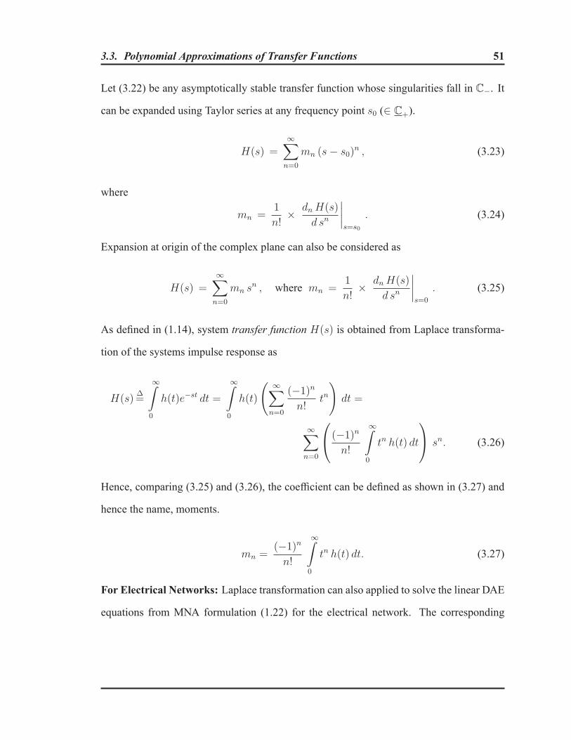
3.3. Polynomial Approximations of Transfer Functions 51
Let (3.22) be any asymptotically stable transfer function whose singularities fall in C−. It
can be expanded using Taylor series at any frequency point s0 (∈ C+).
H(s) =∞∑n=0
mn (s− s0)n , (3.23)
where
mn =1
n!× dnH(s)
d sn
∣∣∣∣s=s0
. (3.24)
Expansion at origin of the complex plane can also be considered as
H(s) =∞∑n=0
mn sn , where mn =
1
n!× dn H(s)
d sn
∣∣∣∣s=0
. (3.25)
As defined in (1.14), system transfer function H(s) is obtained from Laplace transforma-
tion of the systems impulse response as
H(s)Δ=
∞∫0
h(t)e−st dt =
∞∫0
h(t)
(∞∑n=0
(−1)n
n!tn
)dt =
∞∑n=0
⎛⎝(−1)n
n!
∞∫0
tn h(t) dt
⎞⎠ sn. (3.26)
Hence, comparing (3.25) and (3.26), the coefficient can be defined as shown in (3.27) and
hence the name, moments.
mn =(−1)n
n!
∞∫0
tn h(t) dt. (3.27)
For Electrical Networks: Laplace transformation can also applied to solve the linear DAE
equations from MNA formulation (1.22) for the electrical network. The corresponding

3.3. Polynomial Approximations of Transfer Functions 52
equations in Laplace Domain is given by (c.f. Chapter 5):
{CsX(s) + GX(s) = BU(s) (3.28a)
Y(s) = LX(s) , (3.28b)
where X(s) ∈ Cn, U(s) ∈ C
m and I(s) ∈ Cp. Combining (3.28a) and (3.28b), the output
Y(s) is related to the inputU(s) through a transfer function as
H(s) = L (G + sC)−1B . (3.29)
Assuming a regular system (defined in 1.1), let s0 ∈ C+ be a properly selected expansion
point at which matrix pencil (G+ s0C) is nonsingular. From (3.29), it is equivalently
H(s) = L (I + (s− s0)A)−1R, (3.30)
where
A � (G + s0C)−1C (3.31)
and
R � (G + s0C)−1B . (3.32)
The j-th moment of the function at s0 is defined as
Mj(s0) = LMj(s0) = LAj R, for j = {0, 1, 2, . . .} . (3.33)
3.3.1 AWE Based on Explicit Moment Matching
Asymptotic waveform evaluation (AWE) algorithm was first proposed in [76], where ex-
plicit moment matching was used based on Padé approximation to obtain a reduced order

3.4. Projection-Based Methods 53
rational function, sharing the few (e.g. m) leading moments with the original system. In
AWE, the Padé approximant is obtained via explicit computation of the first 2m moments
of H(s) [39, 77, 78]. The AWE method shows that the wildly popular interconnect delay
model, the Elmore delay [79], is just the first order of moments of a circuit. We have to
keep in mind that, (a) accuracy cannot be guaranteed in the whole domain and (b) the AWE
method is numerically unstable for higher-order moment approximation. [39] introduced
some remedial methods to overcome this problem by frequency shifting and expanding
around s = ∞. A more effective method introduced in [80]. It is based on (a) carrying outthe multiple-point expansions along the imaginary axis (called frequency hopping) and (b)
combining the expansion results which takes higher computational costs.
3.4 Projection-Based Methods
In Sec. 3.3.1, we tried to find a direct approximation of the transfer function by explicitly
matching m leading moments. However, explicit moment matching approaches (namely
AWE) suffer from numerical ill-conditioning in their equations. A more elegant solution to
the numerical problem of AWE is to use projection based model order reduction methods,
which are based on implicit moment matching [65]. There are several numerically stable
methods based on the projection on subspaces and implicit moment matching [81–85].
The idea is to first reduce the number of state variables by projecting the vector of state
variablesX on a subspace spanned by the column vectors of an orthogonal matrixQwhose
dimension m � n, where n is the original order. Let there exist z variables in reduced
space such that it can be projected back to the original space with a minimal error ζ(t), as
x(t) = Qz(t) + ζ(t), (3.34)

3.4. Projection-Based Methods 54
where at any time, x(·) ∈ Rn and Qz(·) ∈ colsp(Q). It is desirable for the error vector
ζ(t) to not have any component in the reduced subspace, i.e. colsp(Q). This requires
confining the error vector ζ(t) to the orthogonal complement subspace of colsp(Q), i.e.
ζ(·) ∈ colsp(Q)⊥, where
colsp(Q)⊥Δ=
{w | w ∈ R
n, wTv = 0, ∀ v ∈ colsp(Q)}. (3.35)
It is straightforward to mathematically establish that, the orthogonal complement of the
column-space ofQ ∈ Rm is the null-space ofQT . It is a set of all possible solution vectors
forQTζ(·) = 0.
Substituting x(t) from (3.34) in (1.22a), we get
Cd
dt(Qz(t) + ζ(t)) + G(Qz(t) + ζ(t)) − Bu(t) = 0 (3.36)
and
Cd
dtQz(t) + GQz(t) − Bu(t) = C
d
dtζ(t) + Gζ(t). (3.37)
Considering x(t) ≈ x = Qz, using this approximated solution x leads to a residual error
as
R(ζ(t))Δ=C
d
dtQz(t) + GQz(t) − Bu(t) = C
d
dtζ(t) + Gζ(t). (3.38)
Multiplying both sides of (3.38) by QT and using the orthogonality property as QTζ(·) =0, we get
QTR(ζ) =(QTCQ
) d
dtz(t) +
(QTGQ
)z(t) − (
QTB)u(t) =
Cd
dtQTζ(t) + GQTζ(t) = 0, (3.39)

3.4. Projection-Based Methods 55
and hence, (QTCQ
) d
dtz(t) +
(QTGQ
)z(t) − (
QTB)u(t) = 0. (3.40)
For this purpose, the idea is simply to make the residual error in the differential equa-
tion (1.22a) small when the approximated solution obtained from the reduced model is
used. This is achieved by making the error vector in solution “orthogonal” to the subspace
spanned by the column vectors in Q (the subspace of the solution z). This is the so-called
Petrov-Galerkin [86, pp. 9] scheme in solving differential equations.
Next, the approximated output is obtained as
y(t) = LTQx(t). (3.41)
For the resulting reduced set of differential equations in (3.40) (reduced order model) and
its associated output equation (3.41)), the reduced MNA matrices are
C = QTCQ, G = QTGQ,
B = QTB, and L = LQ . (3.42)
The next step in any subspace projection techniques is to find a proper choice for orthogonal
basis to span the reduced projection space as Q = [q1, q2, . . . ,qm] ∈ Rn×m such that,
having Z ∈ colsp(Q) a properly accurate approximation as X ≈ QZ can be derived.
It is possible to use eigenvectors when digonalization of the dynamic matrix in minimal
state-space representation is possible. Another approach could be to compute the basis
using time series data from all states of systems (in POD [41], [44, Chap.5], [66, Chap.10],
[87]). Alternatively, one may try balancing the system’s controllability and observability
Gramians (in TBR [88]) by using singular value decomposition (SVD) to choose theQ.
Among all the possibilities, the use of Krylov-subspaces is also worth studying.

3.4. Projection-Based Methods 56
3.4.1 General Krylov-Subspace Methods
The most successful algorithms for reduction of large-scale linear systems have been
projection-based approaches [64, 89, 90]. Among all, the (block) Krylov subspace based
projection method [64, 82, 84, 90, 91] is the most commonly used method in model order
reduction. The orthogonal projection matrix that maps the n-dimensional state space of
original system into am-dimensional subspace is constructed as follows:
colsp{Q } = Km (A, R) (3.43)
= span{R, AR, . . . , Am−1R
},
forA andR defined in (3.31) and (3.32). A linear system of much smaller order is derived
by a variable change as x = Qz and multiplying QT on both sides of the differential
matrix equations of reduced variables. For the moment preservation properties for the
Krylov-subspace based methods [90, Theorem-31, pp.36] can be consulted.
3.4.1.1 Arnoldi Algorithm
The Arnoldi method is the classic method to find a set of orthonormal vectors as a basis
for a given Krylov subspace in (3.43). The Arnoldi process was originally introduced in
the field of mathematics by W.E. Arnoldi in 1951 [92]. The Arnoldi algorithm for the ap-
plications in model order reduction of RLC network was introduced in [93]. Given Krylov
subspace Km (A, R), the Arnoldi method using the “modified Gram-Schmidt” orthogo-
nalization [94] calculates the columns of projection matrices. The Arnoldi algorithms is
known to be a numerically efficient iterative method. For the practical implementations of
Arnoldi (SISO) and Block-Arnoldi (MIMO) algorithms, one can refer to [47, 64, 65, 94].

3.4. Projection-Based Methods 57
3.4.1.2 Padé via Lanczos (PVL)
Although the Krylov subspace method (using Arnoldi process) possibly is the widely em-
ployed one, the Padé via Lanczos (PVL) method was the first projection-based method [81].
The classical Lanczos process [95] is an iterative procedure for the successive reduction of
any square matrix to a sequence of tridiagonal matrices. It is a numerically stable method
to compute eigenvalues of generalizable matrices. Lanczos is employed to compute the
Krylov subspace in PVL in the sense of an oblique projection. Later it was proved that the
reduced system implicitly matches the original system to a certain order of moments [96].
Later on, the multiport Padé via Lanczos (MPVL) algorithm [97] was developed which
is an extension of PVL to general multiple-input multiple-output systems. The MPVL
algorithm computes a matrix Padé approximation to the matrix-valued transfer function
of the multiple-input multiple-output system, using Lanczos-type algorithm for multiple
starting vectors [98].
The PVL method was also extended to deal with circuits with symmetric matrices by
means of the SyPVL algorithm [99]. Similarly, its multiport counterpart (SyMPVL) was
introduced in [100].
3.4.1.3 PRIMA
On the idea of utilizing the Krylov subspace, PRIMA (passive reduced-order interconnect
macromodeling algorithm) was introduced in [85] as a direct extension of the block Arnoldi
technique. PRIMA guarantees passivity in the resulting reduced model. The attraction of
the method is mainly due to its passivity preservation which is promised with simple for-
mulation. To shed more light on the method, let (1.22) be the time-domain MNA equations
for a given linear RLC dynamic (MIMO) system, where in susceptance matrix C and con-
ductance matrixG the rows corresponding to the current variables are negated [85]. Also,

3.4. Projection-Based Methods 58
for a p-port system (i.e. m = p) of size n, u(t) and y(t) are the column vectors, including
the voltage sources and the output currents at p ports, respectively. The input matrix B
is a selector matrix consisting of “1”s, “-1”s and “0”s and is related to the output selector
matrix LT = B. By exploiting an orthogonal projection matrix Q, defined by the ba-
sis from Krylov subspace, a change of variable z = QTx is applied in (1.22) to find a
reduced-order model based on a congruence transformation as:
⎧⎨⎩Cd
dtz(t) + G z(t) = B u(t), (3.44a)
y(t) = Lz(t). (3.44b)
The reduced model while preserving the main properties of the original system provides an
output y(t) that appropriately approximates the original response y(t). For the resulting
macromodel in (3.44), the reduced MNA matrices are
C = QTCQ, G = QTGQ,
B = QTB, and L = LQ. (3.45)
It is proved that the reduced system (3.44) of order q preserves the first⌊q/p
⌋block mo-
ments of the original network (1.22) [64, 85]. This implies that for a desired predefined
accuracy, the order of the reduced system should be increased with the increase in the
number of ports p.
3.4.2 Truncated Balance Realization (TBR)
One of the alternative methods for model order reduction of LTI systems is by means of
control-theoretical-based truncated balance realization (TBR) methods [65, 88, 101–116].
In TBR which is a SVD-based approach, the weak uncontrollable and unobservable state

3.4. Projection-Based Methods 59
variables are truncated to achieve the reduced models for linear VLSI systems. For a formal
definition of controllability and observability any references in the area of linear system
theory can be fruitfully consulted with [5, Chapter 6], [57, Chapter 3], and [58, Chapter 9].
3.4.2.1 Standard / Conventional TBR
The TBR procedure is centered around information obtained from the controllability Gram-
mianWc and the observability GrammianWo. These two Gramians are Hermitian pos-
itive definite matrices that can be uniquely [88, 101] obtained from solving the following
Lyapunov equations. Given a state-space model in descriptor form as shown in (3.1), let
E = I. This is as a matter of convenience, while formulation for singular E is also possible
(cf. generalized Lyapunov equation (3.8) in Theorem-3.6).
AWc + WcAT = −BBT (3.46a)
AT Wo + WoA = −CCT (3.46b)
The eigenvalues λ(WcWo) are called the Hankel singular values. In particular “small”
Hankel singular values correspond to internal dynamic modes that have a weak effect on
the input-output behavior of the system and are therefore, close to non-observable or non-
controllable or both [65].
A complete TBR algorithm [103] is shown as Algorithm 1.
Balancing transformation matrixT is obtained in step-5 (of Algorithm 1). Under a similar-
ity transformation, as shown in step-6 a balanced system is obtained whose both Gramians
become equal and diagonal as
Wc = Wo = Σ = diag(σ1, σ2, . . . , σn) , where σ1 ≥ σ2 ≥ . . . ≥ σn. (3.47)

3.4. Projection-Based Methods 60
Algorithm 1: Standard TBR Algorithm.input : Original Model (A, B, C, D)
output: Reduced Macromodel (A, B, C, D)
1 Solve AWc + WcAT = −BBT for Wc ;
2 Solve AT Wo + WoA = −CCT for Wo;3 Compute Cholesky factors Wc = Lc L
Tc and Wo = Lo L
To ;
4 Compute SVD of Cholesky factorsUΣVT = LTo L, where Σ is diagonal positive
andU,V have orthonormal columns;5 Compute the balancing transformation matricesT = LcVΣ−1/2, T−1 = Σ−1/2UTLT
o ;6 Form the balanced realization as A = T−1AT, B = T−1B, C = CT;7 Select reduced model order and partition A, B and C conformally;8 Truncate A, B and C to form the reduced realization A, B, C and it is D = D;
One may partition Σ into
Σ =
⎡⎢⎢⎢⎣ Σ1 0
0 Σ2
⎤⎥⎥⎥⎦ , (3.48)
where the singular values Σ1 = diag(σ1, . . . , σm) and Σ2 = diag(σm+1, . . . , σn). It is
seen that, Σ1 corresponds to the “strong” sub-systems to be retained and Σ2 the “weak”
sub-systems to be deleted [111]. Conformally partitioning the transformed matrices as
A =
⎡⎢⎢⎢⎣ A11 A12
A21 A22
⎤⎥⎥⎥⎦ , B =
⎡⎢⎢⎢⎣ B1
B2
⎤⎥⎥⎥⎦ , C1 =
[C1 C2 .
](3.49)
Hence, the reduced model is defined as
A = A11 , B = B1 , C = C1 . (3.50)

3.4. Projection-Based Methods 61
Error Bounds
One of the attractive aspects of TBR methods is that computable error bounds are available
for the reduced model. This bounded model reduction error is the prominent characteristic
for TBR in comparison to the projection methods based on the (explicit) moment matching,
namely Krylov subspace methods. The error in the transfer function of the order-reduced
model is bounded by [101,102]:
σm ≤∥∥∥H(s) − H(s)
∥∥∥∞
≤ 2n
Σi=m+1
σi . (3.51)
Computational Complexity
For a macromodel of orderm (m << n), the CPU cost is analyzed in the Table 3.1.
Table 3.1: Time complexities of standard TBR.
Operation Cost
Computation of the GramiansWc andWo O (n3)by solving Lyapunov equations in steps 1-2
Two Cholesky decomposition in Step-3∗ 2O (nβ
)(for sparse equations) (typically, 1.1 ≤ β ≤ 1.5)
SVD in Step-4 to computem leading singular values∗ O (nm2)
Linear matrix solving tasks O (nα)(for sparse equations) (typically, 1.1 ≤ α ≤ 1.2)
Forming transformation matrices in step-5 O (nm2)
Similarity transformation in step-6 O (nm)
Total cost: O (n3 + nβ + nm2 + nm
)∗ Based on the algorithms in [117].
It is seen that, the computational cost for solving Lypunov equations O(n3) is dominant.

3.4. Projection-Based Methods 62
Hence, the bottleneck in balanced truncation methods is the computational complexity for
solving the Lyapunov equations. There are both direct and iterative ways to solve Lyapunov
equations. Specifically, the efficient numerical solvers in [108, 109, 118] and newly devel-
oped method in [119] can be named. They are based on the alternated direction implicit
(ADI) method [120, 121]. Despite all the advancement in solution techniques, the com-
plexity cost for solving Lyaponov equations is still noticeably high, prohibiting the TBR
method from reducing large systems.
It is generally remarked that, the TBR methods can produce nearly optimal models but
they are more computationally expensive than projection-based methods.
3.4.2.2 Passive Truncated Balance Realization
To preserve passivity in TBR the following two cases should be considered.
Positive Real TBR (PR-TBR)
The positive-real lemma, states thatH(s) is positive real if and only if there exist matrices
Xc = XTc ≥ 0 , Jc, Kc as well as Xo = XT
o ≥ 0 , Jo, Ko such that the following two
sets of Lur’e equations are satisfied [122].
AXc + XcAT = −KcK
Tc , (3.52a)
XcCT − B = −KcJ
Tc , (3.52b)
Jc JTc = D+DT , (3.52c)
and its dual set,
ATXo + XoA = −KTo Ko , (3.53a)
XoB − CT = −KTc J , (3.53b)
JTo Jo = D + DT . (3.53c)

3.4. Projection-Based Methods 63
Matrices Xc and Xo are analogous to the controllability and observability Gramians, re-
spectively.
Algebraic Riccati Equations (ARE)
By combining (3.52a), (3.52a) and (3.52a) and similarly by combining (3.53a), (3.53a) and
(3.53a), the following two equations (3.54a) and (3.54b) are respectively obtained. They
are so-called, algebraic Riccati equation (ARE) [123].
AXc + XcAT + (B − XcC
T)(D + DT)−1(B − XcCT )T = 0 , (3.54a)
AT Xo + XoA + (CT − XoB)(D + DT)−1(CT − XoB)T = 0 , (3.54b)
The algorithm for positive-real TBR [111,112] is shown as Algorithm 2.
Similar to the standard TBR method, this method also has error bounds.
Algorithm 2: Positive -Real TBR (PR-TBR) Algorithm.input : Original Model (A, B, C, D)
output: Reduced Macromodel (A, B, C, D)
1 Solve set of equations (3.52) ( or equivalently (3.54a) ) for Xc ;2 Solve set of equations (3.53) ( or equivalently (3.54b) ) for Xo ;3 Proceed with steps 3-8 in Algorithm 1, substitutingXc forWc andXo forWo;
Bounded Real TBR (BR-TBR)
As previously explained, passivity for the systems identified by their s-parameters repre-
sentation is ensured by preserving the bounded realness in the order reduction process. To
guarantee the bounded realness of the reduced model H(s) from TBR, a similar procedure
to PR-TBR is followed. It mainly includes obtaining the two system Gramians by solving
the two sets of modified Lur’e equations, so-called bounded-real equations. For further
details, [111] can be consulted with.

3.4. Projection-Based Methods 64
3.4.2.3 Other Extensions of TBR
Spectrally Weighted Balanced Truncation (SBT)
Enns [102, 105] extended the TBR method to include frequency weightings. The resulting
method is known as the frequency weighted balanced truncation. In this method, by using
a chosen weighting function, the error in the reduced model can be minimized and bounded
[106] in some frequency range of interest. With only one weighting present, the stability of
reduced-order models is guaranteed. However, in case of double-sided weightings, Enns’
method may yield unstable models for stable original systems. Several modifications to
Enns’ technique have been proposed to overcome this shortcoming. Wang’s technique
[107, 124], in addition to guaranteeing stability in the case of double-sided weightings,
also provide frequency response error bounds. Generalization of this technique to include
passivity preservation was presented in [116].
Poor Man’s TBR (2005)
An empirical TBR method, named poor man’s TBR, was proposed to improve the scalabil-
ity of the TBR methods, which shows the connection with the generalized projection-based
reduction methods [113,114].
3.4.3 Proper Orthogonal Decomposition (POD) Methods
Proper orthogonal decomposition (POD), also known as Karhunen-Loéve decomposi-
tion [125] or principal component analysis (PCA) [126], provides a technique for ana-
lyzing multidimensional data. It is also a method that derives reduced models by lin-
ear projection. This method essentially constructs an orthonormal projection basis form
the snapshots of the state vectors at N different time-points to form a data matrix as

3.4. Projection-Based Methods 65
X = [x(t1), x(t2), . . . ,x(tN)] ∈ Rn×N , where generally N << n. These time sam-
ples of states are obtained during a transient simulation of the system with some input
excitation [127]. After obtaining the projection matrix from POD approaches, it is used
to generate a reduced model via a standard projection scheme. More details on the time-
domain POD and its formulation are presented in the next chapter.
3.4.3.1 Frequency-Domain POD
For linear (LTI) systems, the POD basis can be obtained efficiently by taking advantage of
linearity and the frequency domain. The frequency-domain POD methods [87, 128–131]
have been developed to obtain reduced model using this frequency domain data. Hence,
in place of transient response, the snapshots of frequency response corresponding to some
frequency points of interest are used. For the problems that applying appropriate time
simulation to obtain snapshots faces difficulties, this frequency-domain approach is well
appreciated. The POD snapshots can, therefore, be obtained by choosing a set of sample
frequencies {ωi} based on the frequency contents of the problems of interest and solvingthe frequency-domain system to obtain the responses X(ωi) = (jωiIn −A)−1
B. The
resulting complex response can be used in a frequency-domain POD analysis as in [128],
or the real and imaginary part of each complex response can be used similar to the snapshots
in a time domain POD analysis as in [131].
The general idea in frequency-domain POD methods is outlined in Algorithm 3.
The benefits of POD methods are the followings.
• The time domain samplesXt = [x(t1), . . . , x(tN)] are easy to obtain using existing
numerical solvers for a system (linear or nonlinear). Extracting the frequency domain
response is also trivially possible using existing solvers. In both cases, one can take
advantage of the sparsity of system matrices and fast solvers.

3.4. Projection-Based Methods 66
Algorithm 3: An Outline of Frequency-Domain POD Algorithm.input : Original Model (A, B, C, D)
output: Reduced Macromodel(A, B, C, D
)1 Select the real frequency points of interest ωk, k = 1, . . . , N ;2 Compute the original system response at frequencies of interestX(ωi) = (jωiIn −A)−1
B for i = 1, 2, . . . , N and store them in an ensemble ofcomplex snapshot,Xs = [X(ω1), X(ω2), . . . , X(ωN)];
3 Construct the correlation matrixR = 1N
(XH
s Xs
), (∈ CN×N );
4 Solve the matrix eigenvalue problem,RTi = λiTi;
5 Form the basis vectors as vi =1N
N∑i=1
TiX(ωi);
6 Construct the projection matrix,V = [v1, v2, . . . ,vm], (m ≤ N ), whose columnvectors span the reduced subspace;
7 Form reduced system’s matrices, A = VTAV, B = VTB, C = CV, and D = D.
• Simple to implement
• In practice, it works quite reliably
• POD does not neglect the nonlinearities of the original vector-field. Indeed, it has a
straightforward generalization for nonlinear systems (see the next chapter)
POD is general because it can take any trajectory of state variables. This advantage of POD
is also its limitation. Because the POD basis is generated from the system response with a
specific input, the reduced model is only guaranteed to be close to the original system when
the input is close to the modeling input. For this purpose, the excitation signals should be
carefully decided such that its frequency spectrum covers the major frequency range of in-
terest for the intended application.
It is worth to remark that, despite the above objection, model reduction via POD is quite
popular and is the method of choice in many fields, mainly due to its simplicity of imple-
mentation and promising accuracy.
3.5. Non-Projection Based MOR Methods 67
3.5 Non-Projection Based MORMethods
Non-projection methods do not employ construction of any projection matrices. The fol-
lowing are several most commonly used methods of this kind.
3.5.1 Hankel Optimal Model Reduction
The task of Hankel optimal model reduction of a matrix transfer function H(s) calls for
finding a stable reduced system H(s) of order less than a given positive integer m, such that
the Hankel norm [101] ‖ζ(s)‖H of the absolute error ζ(s) = H(s) − H(s) is minimal.
Since Hankel operator H represents a “part” of the total LTI system with transfer matrix
H(s), Hankel norm is never larger than L∞ norm. Hence, Hankel optimal model reduction
setup can be viewed as a relaxation of the “original” (L∞ optimal) model reduction formu-
lation. While no acceptable solution is available for the L∞ case, Hankel optimal model
reduction has an elegant and algorithmically efficient solution [101,132–135].
3.5.2 Singular Perturbation
As it will be shown in Chapter 6, projection-based MOR methods can be interpreted as
performing a coordinate transformation of the original system’s state space to a lower di-
mension subspace. For example, in TBR, such space transformation leads to a balanced
system for which we “truncate” the system’s states. This mathematically can be seen as
effectively setting the last (n−m) states to zero. As an alternative, one can instead set the
derivatives of the states to be discarded to zero. This procedure is called state residualiza-
tion, which is the same as a singular perturbation approximation [48]. For more details
and the mechanics of the method, [48, 63] can be consulted. For the basic properties of
singular perturbation for balanced systems, [136] can be referred to.

3.5. Non-Projection Based MOR Methods 68
3.5.3 Transfer Function Fitting Method
With the ever increasing operating frequencies, obtaining analytical models for high-speed
modules becomes difficult and consequently, the characterization based on terminal re-
sponses (obtained through measurements or EM simulations) becomes increasingly popu-
lar [137]. Beside time-domain characterization, linear devices and subsystems can also be
characterized in frequency domain, which is usually more feasible in applications. Such
approaches demand development of fast and accurate physical system identification algo-
rithms so as to embed the resulting model in a transient simulation environment. In order to
make time-domain simulations feasible, one can construct a state-space model that approx-
imates the sampled transfer function of the system. Such methods can be treated as model
reduction, as starting from a characterization of the original system, we obtain a minimal
model as an approximant.
The following methods fall into this category.
3.5.3.1 Rational Fitting Methods
For linear time invariant (LTI) systems, these methods are used to find polynomial coef-
ficients of the numerator and the denominator of approximate rational transfer functions
through iterative application of linear least squares [138].
3.5.3.2 Vector Fitting Methods
Several algorithms have been developed in the recent years for physical system identifi-
cation of networks characterized by tabulated data. One of the popular techniques among
these is the Vector Fitting (VF) algorithm. The vector fitting method was originally in-
troduced in [139] and its extension in [140] to work with frequency domain data. Later,
the method was extended in [141–143] to utilize the time domain data directly. Recently,

3.5. Non-Projection Based MOR Methods 69
in [144, 145] the z-domain vector-fitting algorithms have also been developed. All these
methods are to obtain reduced order (and generally minimal) models for the physical sys-
tems based on the iterative application of Linear Least Squares (LLS), where unknowns
are systems’ poles and residues. Starting with an initial guess of poles, an accurate set of
poles is computed by fitting a scaled function trough pole relocation iterations. After the
poles have been identified, the residues of the transfer function are finally calculated by
solving the corresponding least squares problem with known poles. Although there is no
convergence proof for these methods, they usually work well in practice.
3.5.3.3 Original Formulation
In the original formulation of vector fitting [139], the objective is to approximate a given
frequency response H(s) with a rational function
H(s) ≈N∑
n=1
kns− pn
+ d + hs (3.55)
where terms d and h are optional. The vector fitting first identifies the poles of H(s) by
solving the following linear problem in the least squares sense
δ(s)H(s) = H(s); (3.56)
with
δ(s) =
N∑n=1
rns− an
+ 1 (3.57)
and
H(s) =N∑
n=1
rns− an
+ d + hs (3.58)
3.5. Non-Projection Based MOR Methods 70
where {an} is a set of initial poles, all poles and residues in (3.57) and (3.58) are real orcome in complex conjugate pairs while d and h are real. The relocated (improved) poles
are equal to the zeros of δ(s) and are obtained as
{an} = eig(A−BCT
)(3.59)
whereA is a diagonal matrix holding the poles {an}, B is a column vector of ones, and Cis a column vector holding the residues rn.
This procedure can be applied in an iterative manner where (3.56)-(3.59) are solved re-
peatedly with the new poles from (3.59). After the poles have been identified, the residues
of (3.55) are finally calculated by solving the corresponding least squares problem with
known poles [139,146].
Later (2006), a modification of the VF formulation was introduced in [147,148], which
improves the ability of VF to relocate poles to better positions, thereby improving its con-
vergence performance and reducing the importance of the initial pole set. This is achieved
by replacing the high-frequency asymptotic requirement of the vector fitting scaling func-
tion (3.57) with a more relaxed condition as
δ(s) =
N∑n=1
rns− an
+ d. (3.60)
Another noteworthy improvement, to speed-up the vector fitting for multiport systems us-
ing a common set of poles was introduced in [149]. This is achieved by applying the QR
decomposition to the LS equations formed in each iteration of VF.

3.5. Non-Projection Based MOR Methods 71
3.5.3.4 Generalized Formulation
In general, the frequency domain VF methods are used to find rational transfer function
H(s) =N(s)
D(s)=
N∑k=1
NkΦk(s)
D∑r=1
DrΦr(s)
s = j2πf (3.61)
which approximates the spectral response of a system over some predefined frequency
range of interest [fmin, fmax]. This reduces to finding the real-valued coefficients Nk, Dr
and the poles for basis functions Φi(s), where the numbers N andD represent the order of
numerator and denominator, respectively.
Rational least-squares approximation is essentially a nonlinear problem, and corresponds
to minimizing the following cost function [140,150,151]
arg minNk,Dr
Nfreq∑l=0
∣∣∣∣H(sl)− N(sl)
D(sl)
∣∣∣∣2 = arg minNk,Dr
Nfreq∑l=0
(1
|D(sl)|2|D(sl)H(sl)−N(sl)|2
).
(3.62)
By taking Levi’s approach [152], the problem is simplified to minimizing the summation of
the squared weighted error as shown below, that is nonquadratic in the system parameters
arg minNk,Dr
Nfreq∑l=0
|D(sl)H(sl)−N(sl)|2 . (3.63)
3.5. Non-Projection Based MOR Methods 72
3.5.3.5 Sanathanan-Koerner
Advocating the Sanathanan-Koerner interactive weighted LLS estimator [153], the model
parameters at the t-th iteration are calculated by minimizing the weighted linear cost func-
tion
arg minNk
(t),Dr(t)
⎛⎝Nfreq∑l=0
1
|D(t−1)(sl)|2∣∣D(t)(sl)H(sl)−N (t)(sl)
∣∣2⎞⎠ (3.64)
where for the first iteration D(0)(s) = 1.
3.5.3.6 Basis Functions for Original VF
In the original VF (Sec. 3.5.3.3), to make sure that the transfer function has real-valued
coefficients, the adopted partial fractions are used as basis functions Φi(s) in (3.61). These
basis are obtained as a linear combination of the partial fractions for any pair of complex
conjugate poles. The adopted nonorthogonal basis functions are
• For real poles, pn = −αn ∈ R:
Φn(s) =1
s− pn(3.65)
• For complex conjugate poles, pn,n+1 = −αn ± jωn, αn, ωn ∈ R:
Φn(s) =1
s− pi+
1
s− p∗i(3.66)
Φn+1(s) =j
s− pn− j
s− p∗n(3.67)
3.5.3.7 Orthonormal Vector Fitting
In [140], the Orthonormal Vector Fitting (OVF) technique was developed to approximate
frequency domain responses. The OVF method uses orthonormal rational functions for

3.5. Non-Projection Based MOR Methods 73
Φi(s) to improve the numerical stability of the method. This reduces the numerical sensi-
tivity of the system equations to the choice of starting poles and limits the overall macro-
modeling time. To ensure the resulting transfer function has real-valued coefficients, the
orthonormal functions in the following format are used
• For stable real poles, pn = −αn ∈ R:
Φn(s) =√
−2pn
(n−1∏i=1
s+ p∗is− pi
)1
s− pn(3.68)
• For stable complex conjugate poles, pn,n+1 = −αn ± jωn, αn, ωn ∈ R:
Φn(s) =√−2�e (pn)
(n−1∏i=1
s+ p∗is− pi
)s+ |pn|
(s− pn) (s− p∗n)(3.69)
Φn+1(s) =√−2�e (pn)
(n−1∏i=1
s+ p∗is− pi
)s− |pn|
(s− pn) (s− p∗n)(3.70)
3.5.3.8 z-Domain Vector Fitting
In [144] z-domain vector-fitting (ZDVF) is proposed to fit transfer functions using fre-
quency or time-domain response data. This method is a reformulation of the original vector
fitting method in the z-domain. It has an advantage of faster convergence and better numer-
ical stability compared to the s-domain VF. The fast convergence of the method reduces
the overall macromodel generation time.
The z-domain response of a dynamic system can be constructed from the the time
domain response or by using s-to-z bilinear transformation. The z-domain response H(z)
of any linear time-invariant passive network can be represented using rational function. For
an D-th order system response, the rational function is
H(z) =N(z)
D(z)=
N∑k=0
bnz−k
D∑r=1
arz−r
=
N∑k=1
NkΦk(z)
D∑r=1
DrΦr(z)
(3.71)

3.5. Non-Projection Based MOR Methods 74
Using the following basis functions conforms to the requirement of real-valued time-
domain response from the resulting transfer functionH(z) (3.71) (or from its equivalent in
s-domain).
• For real poles, pn = αn ∈ R and |Pn| < 1:
Φn(z) =1
z − pn(3.72)
• For complex conjugate poles, pn,n+1 = αn ± jβn, αn, βn ∈ R and |Pn| < 1:
Φn(z) =1
z − pi+
1
z − p∗i(3.73)
Φn+1(z) =j
z − pn− j
z − p∗n(3.74)
3.5.3.9 z-Domain Orthonormal Vector Fitting
An advanced macromodeling tool based on z-domain Orthonormal Vector Fitting (ZD-
OVF) was developed in [145, 154] for fast and accurate macromodeling of linear subnet-
works using either frequency or time-domain tabulated data. This algorithm extends the
inherent advantages of orthonormal basis to z-domain VF formulations. Hence, it further
improves the numerical stability of the ZVF method and significantly reduces the numer-
ical sensitivity of the system equations to the choice of starting poles. This directly leads
to an improvement of the overall macromodeling time. To this end, the following modified
z-domain Takenaka-Malmquist orthonormal bases are developed.
• For real poles, pn = αn ∈ R and |Pn| < 1:
Φn(z) =
√1− |pn|2
(n−1∏i=1
1− p∗i z
z − pi
)1
z − pn(3.75)
• For complex conjugate poles, pn,n+1 = αn ± jβn, αn, βn ∈ R and |Pn| < 1:
Φn(s) =1√2|1 + pn|
√1− |pn|2
(n−1∏i=1
1− p∗i z
z − pi
)1− z
(z − pn) (z − p∗n)(3.76)
3.5. Non-Projection Based MOR Methods 75
Φn+1(s) =1√2|1− pn|
√1− |pn|2
(n−1∏i=1
1− p∗i z
z − pi
)1 + z
(z − pn) (z − p∗n)(3.77)
3.5.3.10 State-Space Realization from Poles and Residues
The real-valued minimal LTI state-space realization (A,B,C,D) using the poles and
residues is an important step in the iterations of the vector fitting methods. It has been
corroborated that the zeros of the denominator expression become the improved poles to
start the next iteration and for the final transfer function. Calculating the zeros can be done
through state-space realization of the denominator. An example was provided for the for-
mulation of original VF in the Sec. 3.5.3.3. For the details of such realizations for other
vector fitting methods, the above corresponding reference can be refereed to. It is to be
noted that, the representation of a transfer function in state-space form is obviously not
unique.
Also, to incorporate the resulting multiport macromodels for subnetworks in higher
level spice-like simulations, generating an equivalent circuit for the macromodels is impor-
tant. This can be achieved in two steps. First a state-space representation is obtained. For
the details [151] and [64, Sec. 7.3] can be referred to. The second step is to synthesize an
equivalent circuit, the details of which can be found in [64, Sec. 7.4].
3.5.3.11 Recursive Convolution
Another way of converting a frequency-domain description to a time-domain model is
through convolution, which, in general, has a quadratic CPU-time cost. If the frequency-
domain descriptions are in terms of poles and residues, we can exploit this fact and evaluate
the convolutions in a recursive manner so that the computational cost is constant regardless
of the time [64]. The recursive convolution method is efficient and easy to implement. For
further details [64, Sec. 7.5] can be referred to.

3.6. Other Alternative Methods 76
3.5.3.12 Quasi-Convex Optimization Method:
This method was originally introduced in [155] and uses more rigorous techniques to obtain
guaranteed stable models. It can be used to obtain parameterized models, which preserve
additional properties such as passivity [156].
3.6 Other Alternative Methods
It is to be noted that, the existing methods are not strictly limited to the presented cate-
gories. There is a variety of recent reduction techniques that have been proposed in the
area of linear MOR. These techniques aim at obtaining the best results by combining ad-
vantages from different methods. As an example, one can consider interpolatory model
reduction techniques [137, Sec.1-7, part I] and [157, 158], which has recently (2012) at-
tracted attention. Interested readers can also consult (e.g.) [83, 87, 112, 159–163] for some
other examples of such techniques.

Chapter 4
Model Order Reduction for Nonlinear
Dynamical Systems
Model order reduction of nonlinear systems follows the model order reduction for linear
systems. However, compared to the reduction of linear systems, nonlinear model reduction
are much less developed and are far more challenging to develop and analyze. The
problem of nonlinear model reduction deals with approximations of the large nonlinear
dynamic systems represented in the form of a nonlinear differential equations. This is
mainly to reduce costs of simulating large systems, a goal that can only be attained trough
answering both the following two sub-problems
a. Reducing the dimensionality of the state vector,
b. Finding ways to efficiently calculate nonlinear functions and derivatives.
While an elaborated formulation of nonlinear systems is presented in Chapter-1, it is con-
cisely revisited here.
For a broad class of engineering problems, the following nonlinear models consisting
of a system of state equations (DAE) (4.1a) along with output equations (4.1b) as shown
77

4.1. Physical Properties of Nonlinear Dynamical Systems 78
below, are ample to represent their nonlinear dynamical behavior.
⎧⎨⎩d
dtg (x(t)) = F (x(t)) + Bu(t), x(t0) = x0 (4.1a)
y (t) = Lx (t) (4.1b)
where system variables x(t) ∈ Rn, nonlinear vector functions g(x), F(x) : Rn �→ R
n,
B ∈ Rn×p, L ∈ R
q×n, u(t) ∈ Rp, and y(t) ∈ R
q. Nonlinear electrical networks can also
be characterized by a set of coupled nonlinear first order differential equations representing
the dynamical behavior of the system variables [21–23, 25, 27, 164–166]. In the context of
circuit simulation, these equations are directly obtained from the circuit netlist using the
modified nodal analysis (MNA) matrix formulation [37–39,167] in the form
⎧⎨⎩Cd
dtx(t) +Gx(t) = F (x(t)) +Bu(t), x(t0) = x0 (4.2a)
y(t) = Lx(t) (4.2b)
where C andG ∈ Rn×n are susceptance and conductance matrices including the contribu-
tion of linear elements, respectively.
4.1 Physical Properties of Nonlinear Dynamical Systems
Similar to the linear case, there are important conditions that, nonlinear differential equa-
tions representing dynamics of a physical systems have to satisfy. It is also desirable to
have such inherent characteristics of the original system passed on to the lower order ap-
proximant obtained in the MOR process. This section reviews some of these important
properties mainly related to the “Lipschitz Continuity” and the “stability” of dynamical
nonlinear systems. The former is the most important condition to ensure the “existence and
uniqueness” of the response for a physical system. The latter is significantly important in

4.1. Physical Properties of Nonlinear Dynamical Systems 79
analyzing the local/global behavior of nonlinear systems.
4.1.1 Lipschitz Continuity
For any given nonlinear system defined in D as an initial value problem in the following
form
x(t) = F ( t, x(t) ) , with x(t0) = x0, (4.3)
existence and uniqueness can be ensured by imposing some constraints on the vector field
function F (t, x) in (4.3). The key constraint for this is Lipschitz condition.
Definition 4.1 (Lipschitz condition [7,168]). Consider the function F (t, x) = [f1 (t, x) ,
f2 (t, x) , . . . , fn (t, x)]T with F : (R× R
n) �→ Rn, |t − t0| ≤ a, and x =
[x2, x2, . . . , xn]T ∈ D ⊂ R
n, where D is an open and connected set; F (t, x) satisfies
the Lipschitz condition with respect to x if in [t0 − a, t0 + a] × D we have
‖F (t, x1) − F (t, x2) ‖ ≤ L‖x1 − x2‖, (4.4)
with x1, x2 ∈ D and L a constant. Positive constant L is called the Lipschitz constant.
Given function F(x) : D �→ Rn is defined in an open and connected set D ⊂ R
n,
and each component of F(x) does not explicitly depend on time. A system of differential
equations having this F(x) as its vector field function, i.e.
x(t) = F (x(t) ) , with x(t0) = x0, (4.5)
is referred to as autonomous system. For autonomous systems (4.5), Lipschitz condition is
also defined in a similar manner to the definition in 4.1.
A locally Lipschitz function on an open and connected domain D is Lipschitz on every

4.1. Physical Properties of Nonlinear Dynamical Systems 80
compact (closed and bounded) subset of D [17]. According to the domain over which theLipschitz condition holds, it is categorized as locally Lipschitz and globally Lipschitz.
A geometrical interpretation for Lipschitz property of function f(x) (f : R �→ R), is
illustrated in Fig. 4.1. It implies that on a plot of f(x) versus x, a straight line joining any
two points of f(x) cannot have a slope (4.6), whose absolute value is greater than L.
|f(x2) − f(x1)||x2 − x1| ≤ L . (4.6)
f(x)
f(x1)
f(x2)
xx1 x2
Figure 4.1: Illustration of Lipschitz property.
4.1.2 Existence and Uniqueness of Solutions
The existence theorem originally contributed by A. L. Cauchy (1789-1857). Since then,
many different forms of existence theorem have been established in the literature of dy-
namical systems.
Theorem 4.1 (Existence-Uniqueness [7]). Consider the initial value problem given in
(4.3) with x ∈ D ⊂ Rn, |t − t0| ≤ 0; D = {x | ‖x − x0‖ ≤ d}, where a and d are
positive constants. The vector function F (t, x) satisfies the following conditions:
4.1. Physical Properties of Nonlinear Dynamical Systems 81
a) F (t, x) is continuous in G = [t0 − a, t0 + a] × D;
b) F (t, x) is Lipschitz continuous in x .
Then the initial value problem has one and only one solution for |t − t0| ≤ min(a, d
M
)withM = sup
G‖F‖.
Proof. For the proof [8, 9, 169] can be referred to. �
4.1.3 Stability of Nonlinear Systems
This section briefly reviews several definitions and results concerning the stability of non-
linear dynamical systems that have been commonly used for the stability analysis of the
reduced nonlinear models in the literature (e.g. [170–174]). For some more details on the
fundamental concepts and definitions of stability analysis, Chapter 2.6.1 can be referred to.
However, it needs to be remarked that, the stability analysis for nonlinear systems is not
nearly as simple as it was for linear systems, presented in Sec. 3.1.1.
Consider the nonlinear dynamical system
x(t) = F (x(t), u(t) ) (4.7)
with equilibrium point xeq such that F (xeq,0) = 0. For (4.7) the local behavior analysis
(cf. Sec. 2.6.2.1) at an equilibrium point turns out to be a less sophisticated task, compared
to the difficulties associated with the global stability analysis (cf. Sec. 2.6.2.2). In order to
determine the local behavior of a nonlinear system at an equilibrium point, it is sufficient to
consider the linearizations of the nonlinear model about that equilibrium point and analyze
the stability of the local approximate model. This is referred to as Lyapunov’s indirect
method.

4.1. Physical Properties of Nonlinear Dynamical Systems 82
Theorem 4.2 (Lyapunov’s indirect method [55, 170]). If the linearized system
x(t) = Ax(t), where A =∂F (x,u)
∂x
∣∣∣∣x=xeq , u=0
(4.8)
is asymptotically stable, then xeq is a locally asymptotically stable equilibrium of the system
(4.5).
Thus, the equilibrium of the nonlinear system is stable if the Jacobian matrixA has eigen-
values with a strictly negative real part.
Consider the nonlinear dynamical system
Cx(t) = F (x(t), u(t) ) , y(t) = Lx, (4.9)
which may arise when modeling analog circuits using modified nodal analysis. Assume
that the descriptor matrix C is nonsingular and the system has a unique equilibrium point
xeq. This equilibrium point is said to be exponentially stable if all solutions to the au-
tonomous system (i.e. u = 0, ∀ t) for any arbitrary initial condition x0 converge to the
equilibrium point exponentially fast. Without a loss of generality we may transform the
coordinate system such that xeq = 0.
Definition 4.2 (Exponentially stable [171]). The equilibrium xeq = 0 is said to be expo-
nentially stable if there exist constants r, a, b > 0 such that
‖x (t0 + t)‖ ≤ a ‖x0‖ e−bt, ∀ t, t0 ≥ 0, ∀x0 ∈ Br ⊆ Rn (4.10)
Here, Br is a ball with radius r centered at xeq.
Exponential stability can be proven through Lyapunov functions.

4.1. Physical Properties of Nonlinear Dynamical Systems 83
Theorem 4.3 ( [170, 175]). The equilibrium point xeq = 0 of system (4.9) is exponentially
stable if there exist constants λ1, λ2, λ3 > 0 and a continuously differentiable Lyapunov
function L(x) such that
λ1xTx ≤ L (x) ≤ λ2x
Tx (4.11)
∂
∂tL (x) ≤ −λ3x
Tx (4.12)
∀t ≥ 0, ∀x ∈ Br ⊆ Rn.
Definition 4.3 (Globally exponentially stable [171]). If Br = Rn (in Def. 4.2 or Theo-
rem 4.3), then the equilibrium point is globally exponentially stable.
External stability refers to the input-output system (4.9) and concerns the system’s
ability to amplify signals from input u to output y. Qualitatively, the system is said to be
externally stable if the system’s output y(t) can be bounded in some measure by a linear
function of the system’s input u(t) in that same measure.
Definition 4.4 (Small-signal finite-gain Lp stable [171, 175]). System (4.9) is said to be
small-signal finite-gain Lp stable if there exist rp > 0 and γp < ∞ such that
‖y‖p ≤ γp ‖u‖p (4.13)
for all t > t0, given initial state x(0) = 0 and input u(t) such that ‖u‖∞ < rp. if rp = ∞,then the system is finite-gain Lp stable.
Theorem 4.4 (Small-signal finite-gain Lp stable [170,175]). Suppose xeq = 0 is an expo-
nentially stable equilibrium of system (4.9). If F (x, u) is continuously differentiable and
F (x, u) is locally Lipschitz continuous at (xex = 0,u = 0), then system (4.9) is small-
signal finite-gain Lp stable.

4.2. Nonlinear Order Reduction Algorithms 84
Definition 4.5 (Finite-gain Lp stable). If a small-signal finite-gain Lp stable system (4.9)
in Theorem-4.4 is globally exponentially stable (Br = Rn), the system is finite-gain Lp
stable.
4.2 Nonlinear Order Reduction Algorithms
In Fig. 4.2 four different classes of the existing model order reduction techniques for non-
linear systems in (4.1) (or its counterpart (4.1)) are displayed.
For Nonlinear Dynamical Systems:
Taylor series based methods:
(1) Linearization
(2) Quadratic reduction
(3) Bilinearization
+ Volterra series
+ Multimoment
Piecewise Trajectory Based
Methods (e.g. TPWL)
Proper Orthogonal
Decomposition
(POD)
Empirical
Balanced
Truncation
(TBR)
Figure 4.2: Model reduction methods for nonlinear dynamical systems categorized intofour classes.
4.2.1 Projection framework for Nonlinear MOR - Challenges
The projection-based approached have been the most successful algorithms for reduction
of large-scale linear systems (cf. Chapter 3 and references therein e.g. [64, 89, 90]). In
contrast, a direct application of the projection framework to the large nonlinear systems
can generally face some challenges. Consider the nonlinear system in (4.1). We may

4.2. Nonlinear Order Reduction Algorithms 85
formally apply the projection recipe to this system of equations which leads to a “reduced”
order system of equations in the following form
⎧⎨⎩d
dtWTg (Vz(t)) = WTF (Vz(t)) + WTBu(t), z0 = Vx(t0) (4.14a)
y (t) ≈ LVz (t) . (4.14b)
First, it is not at all clear how to choose left and right projection matricesW and V, and
even less is known about efficient computation of the response from the resulting models.
In the general case, interpreting the termsWTg (Vz(t)) andWTF (Vz(t)) as “reduced”
models is problematic. Since g (x) and F (x) are nonlinear function, the only way to
computingWTg (Vz(t)) andWTF (Vz(t)) may be to (1) explicitly construct x = Vz,
(2) evaluate g = g (x) and F = F (x), and (3) compute WTg and WTF. As a result,
an efficient simulation is not guaranteed. For example, in a nonlinear circuit simulation,
even for circuits with tens of thousands of nodes, roughly half the simulation time is spent
on evaluating the nonlinear functions g (x) and F (x) . Thus, regardless of the reduction
in the size of the state space, since the original nonlinear functions must be evaluated, the
efficiency gained from the order reduction will be at most a factor of two or three [176].
Consequently, in order to obtain efficient, low-cost reduced order models for nonlinear
systems the following two issues need to be addressed by a MOR technique:
(a) Constructing low-order projection basisW andV, which approximate the dominant
(’useful’) parts of the state-space to accommodate the dynamics of the system
(b) Applying the low-cost, yet feasible approximate representation of system’s nonlin-
earity (associated with g (x) and F (x)).
The first of the issues is developing suitable projection bases for linear systems. This has
received a considerable amount of attention, leading to successful approaches based (e.g.)
on Proper Orthogonal Decomposition that is explained in the Sec. 4.2.4. The techniques

4.2. Nonlinear Order Reduction Algorithms 86
such as linearization, quadratic methods presented in Sec. 4.2.2, and TPWL approach in
Sec. 4.2.3 are used to address the problem of finding cost-efficient representations of non-
linearity.
4.2.2 Nonlinear Reduction Based on Taylor Series
The very first practical approaches to nonlinear model reduction were based on using Tay-
lor series expansions of nonlinear functions F(x(t)) and g(x(t)) in [42, 176–180]. The
original system should be expanded around some (initial, equilibrium) state x0 on a rep-
resentative trajectory, using a multidimensional Taylor series expansion technique. The
Taylor expansion of the functions are
F(x) = F(x0) + G1 (x− x0) + G2 (x− x0)⊗ (x− x0) +
G3 (x− x0)⊗ (x− x0)⊗ (x− x0) + . . . (4.15)
and
g(x) = g(x0) + C1 (x− x0) + C2 (x− x0)⊗ (x− x0)+
C3 (x− x0)⊗ (x− x0)⊗ (x− x0) + . . . (4.16)
where ⊗ is the Kronecker product, C1 =∂
∂xg
∣∣∣∣x0
and G1 =∂
∂xF
∣∣∣∣x0
(∈ Rn×n) are the
Jacobian matrices and C2, G2 (∈ Rn×n2
) are Hessian tensors that represent the second
order contributions and in general Ck, Gk (∈ Rn×nk
) correspond to tensors with the k-th
order effect contributions.

4.2. Nonlinear Order Reduction Algorithms 87
4.2.2.1 Linearization Methods
Linearization is the earliest and most straightforward approach to model nonlinear systems.
In this approach, the strategy is based on linearizing the system around some point in its
state-space. For this purpose, F(x) and g(x) are assumed to be smooth enough so that
it can be expanded into Taylor series. This means that the sum of infinite terms in (4.15)
and (4.16) are truncated to only the first order terms or linear components. Substituting the
truncated approximant series for F(x) (4.15) and g(x) (4.16) in (4.1), we get
d
dt(g(x0) + C1 (x− x0)) = F(x0) + G1 (x− x0) + Bu(t) (4.17)
and next,
C1d
dtx = G1x − G1x0 + F0 + Bu(t) (4.18)
where F0Δ= F(x0).
It can be equivalently rewritten as
C1d
dtx = G1x +
[B, F0 −G1x0
]︸ ︷︷ ︸
B
⎡⎢⎢⎢⎣u(t)1
⎤⎥⎥⎥⎦︸ ︷︷ ︸
u(t)
. (4.19)
It is desirable to matchmmoments of the transfer function of the reduced model with those
of the transfer function of the original system (4.19) at the complex frequency point s0. For
this purpose, the projection matrix for order reduction is constructed using the Arnoldi
algorithm based on the Krylov subspace as follows
colspan{V} = Kr {A,R} = span {R,AR, . . . , AmR} , (4.20)

4.2. Nonlinear Order Reduction Algorithms 88
whereR Δ= (s0C1 −G1)
−1B andA Δ
= (s0C1 −G1)−1
C1.
Using the projection matrix V and a variable change as x(t) = Vz(t), the reduced lin-
earized model is
⎧⎨⎩Cd
dtz(t) = G z(t) + B u(t), (4.21a)
y(t) = Lz(t), (4.21b)
where
C = VTC1V, G = VTG1V,
B = VTB, L = LV. (4.22)
4.2.2.2 Quadratic Methods
Quadratic method is an improvement over the previous approach (cf. Sec. 4.2.2.1) where
the second order term of the expansion in (4.15) is also included for the state-space approx-
imation of the nonlinear system. Given x0 = 0 as the expansion point, the approximants
for nonlinear functions in (4.1) are
F(x) ≈ F(0) + G1x + xTG2x, and g(x) ≈ g(0) + C1x. (4.23)
whereC1 andG1 are the Jacobian of g and F , respectively, evaluated about origin andG2
is an n× n2 Hessian tensor whose entries are given by
g2 i,j,k =1
2
∂2fi∂xj∂xk
. (4.24)

4.2. Nonlinear Order Reduction Algorithms 89
and hence,
C1d
dtx = G1x + xTG2x +
[B, F0
]︸ ︷︷ ︸
B
⎡⎢⎢⎢⎣u(t)1
⎤⎥⎥⎥⎦︸ ︷︷ ︸
u(t)
. (4.25)
Having a desirable projection matrixV, the reduced model is
VTC1Vd
dtz = VTG1Vz + VTzTVTG2Vz + VTBu(t). (4.26)
In tensorial notation, it can be equivalently rewritten as
(VTC1V
) d
dtz =
(VTG1V
)z + VTG2 (V ⊗V) (z⊗ z) +
(VTB
)u(t), (4.27a)
y(t) ≈ LVz(t). (4.27b)
From the reduction process above, it is seen that the quadratic method is more precise
than the traditional linearization method. To obtain the projection matrix V, the simple
approach is to consider the Krylov subspaces defined by the linear part of the representation
by ignoring the second order term. There are also specially designed methods for the
extraction of the projection matrix, known as the quadratic projection methods [42, 180–
183]. They are based on considering the effect of the linear and second order components
in Taylor series expansion for defining the corresponding Krylov subspace and to construct
the orthogonal vector basis.
4.2.2.3 Bilinearization Reduction Method
This section reviews the bilinearization reduction method based on the approach proposed
in [176]. This method uses the terms from the Taylor expansion in (4.15) up to the quadratic

4.2. Nonlinear Order Reduction Algorithms 90
term to approximate the nonlinear functions. For simplicity of description, consider the
expanded state-space model of the nonlinear system as
d
dtx = G1x + G2x⊗ x + Bu(t), y(t) = Lx. (4.28)
Following the computational steps in [176,184] an approximate bilinear system is obtained
asd
dtx⊗ = A⊗x⊗ + N⊗x⊗ + B⊗u(t), y(t) = L⊗Tx, (4.29)
where
x⊗ =
⎡⎢⎢⎢⎣ x
x⊗ x
⎤⎥⎥⎥⎦ , B⊗ =
⎡⎢⎢⎢⎣ B
0
⎤⎥⎥⎥⎦ , L⊗ =
⎡⎢⎢⎢⎣ L
0
⎤⎥⎥⎥⎦ , (4.30)
A⊗ =
⎡⎢⎢⎢⎣ G1 G2
0 G1 ⊗ I+ I⊗G1
⎤⎥⎥⎥⎦ , N⊗ =
⎡⎢⎢⎢⎣ 0 0
B⊗ I+ I⊗B 0
⎤⎥⎥⎥⎦ . (4.31)
The resulting bilinear systems (4.29) is of much larger dimension than the original non-
linear system. For bilinear systems, Volterra-series expression [185] and multimoment
expansions [176] are the key to applying the Krylov subspace based MOR. For further
details [184, 186] can be referred to.

4.2. Nonlinear Order Reduction Algorithms 91
4.2.3 Piecewise Trajectory based Model Order Reduction
The main drawback of Taylor-series based MOR methods for nonlinear systems is that
these methods typically expand the nonlinear operator about a single state (cf. Sec-
tions 4.2.2.1, 4.2.2.2, and 4.2.2.3). Therefore the generated models are only accurate lo-
cally, a fact that makes them useful only for weakly nonlinear systems. In order to over-
come this weak nonlinearity limitation, TPWL approach was first proposed in [187] and
then extended in several ways (e.g.) [171, 172, 188–198]. The central idea in all these
approaches is to use a collection of expansions around states visited by a given training
trajectory. Hence, one may categorize them in a class of methods that can be referred to as
“piecewise trajectory based” methods.
TPWL: The idea in TPWL [187, 188, 199] is to represent a nonlinear system as a collage
of linear models in adjoining polytopes, centered around expansion points xi, in the state
space as illustrated in Fig. 4.3.
Given a nonlinear system as shown below
⎧⎨⎩Cd
dtx(t) = F (x(t)) + Bu(t), x(t0) = x0 (4.32a)
y (t) = Lx (t) . (4.32b)
For the sake of simplicity in the form of equations for TPWL, in (4.32), we considered
g (x) = C, whereC is a constant matrix. The steps ofTPWL approach can be summarized
as follows.
1. Finding the nonlinear system trajectory in response to a properly chosen training
input.
2. Locating meaningful states as linearisation points (LPs) along the trajectory at which
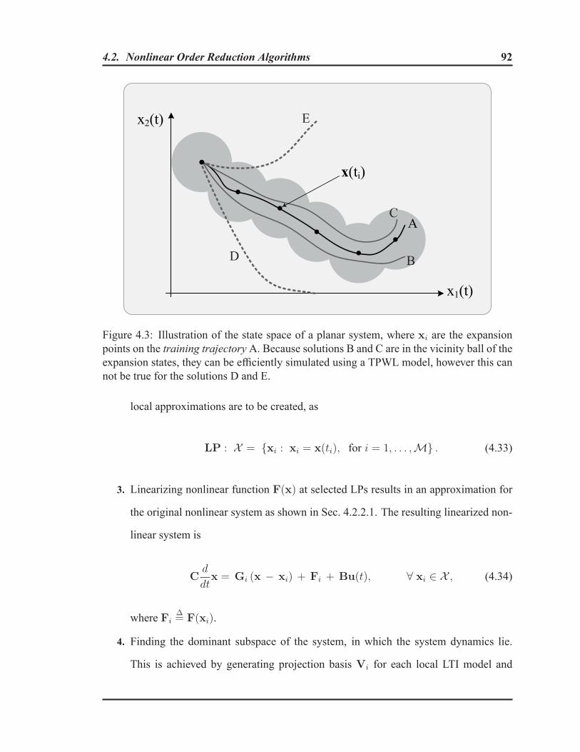
4.2. Nonlinear Order Reduction Algorithms 92
x1(t)
x2(t)
x(ti)
A
B
C
D
E
Figure 4.3: Illustration of the state space of a planar system, where xi are the expansionpoints on the training trajectory A. Because solutions B and C are in the vicinity ball of theexpansion states, they can be efficiently simulated using a TPWL model, however this cannot be true for the solutions D and E.
local approximations are to be created, as
LP : X = {xi : xi = x(ti), for i = 1, . . . ,M} . (4.33)
3. Linearizing nonlinear function F(x) at selected LPs results in an approximation for
the original nonlinear system as shown in Sec. 4.2.2.1. The resulting linearized non-
linear system is
Cd
dtx = Gi (x − xi) + Fi + Bu(t), ∀ xi ∈ X , (4.34)
where FiΔ= F(xi).
4. Finding the dominant subspace of the system, in which the system dynamics lie.
This is achieved by generating projection basis Vi for each local LTI model and

4.2. Nonlinear Order Reduction Algorithms 93
calculating a common subspace V through aggregation of the local subspaces as
Vagg = {V1, V2, . . . , VM}. Then, reorthogonalization of the column vectors inVagg using SVD construct a new basis V. The order of the global reduced subspace
colspan (V ) is usually larger than each Vi but much smaller than the size of the
original system.
5. Performing the linear model reduction usingV on the local linear submodels and the
output equation,
Cd
dtz = G (z − zi) + Fi + Bu(t), ∀ xi ∈ X , y(t) ≈ Cz, (4.35)
where
C = VTCV, B = VTB, L = LV,
Gi = VTGiV, Fi = VTF(xi). (4.36)
6. The final reduced model is the weighted combination of all the reduced models
Cd
dtz =
M∑i=1
ωi (z)(Gi (z − zi) + Fi + Bu(t)
), y(t) ≈ Cz, (4.37)
where ωi (z) is the weighting function.
On the reduction of the linear submodels: In the steps-4 and 5, basically, any MOR-
technique for linear problems can be applied to the linear submodels. In the original ap-
proach [199], a Krylov-based reduction using the Arnoldi-method was proposed. [189]
introduced Truncated Balanced Reduction (TBR) to TPWL and [200] proposed using Poor
Man’s TBR. Proper Orthogonal Decomposition (POD) was also used in [194] as linear
MOR kernel. For comparison of different linear MOR strategies when applied to problems

4.2. Nonlinear Order Reduction Algorithms 94
in circuit simulation [201–204] can be referred to.
Determination of the weights: In the step-6, the method deals with the combination of
weighted reduced linear submodels. To ensure, and at the same time, to limit the dominance
of each submodel to its own segment, the weighting functions of choice naturally require
to have steep gradients. To this end, the original work in [199] suggested a scheme that is
depending on the absolute distance of a state to the linearization points. The importance of
each single model is weighted by
ωi (x) = e−βγ‖x−xi‖2 , with γ = min
i‖x− xi‖2 . (4.38)
where β decides the pace of the decay for weighting functions. A typical value may be
chosen as β = 25. To guarantee a convex combination, the weights are normalized such
that∑i
(x) = 1.
The TPWL has excellent global approximations for large signal analysis because of
the piecewise nature but has limited local accuracy for small signal analysis. Intuitively,
when the excitation is small enough to keep the states stay within one region, the system
reduces to a pure LTI model, and no distortions could be captured. Nonlinearities induced
exclusively by the nonlinear weight function ωi (z) are generated only when states cross
boundaries. Recently, some works [191–193] have greatly extended the original TPWL
method, making it more scalable and practical. However, there is still less evidence in
literature to show the usage of the generated macromodel in other analysis, such as dc, ac,
HB, etc. [196].
TPWP: To address the above shortcomings, a method proposed in [196]. It combines the
trajectory-based techniques and the weakly nonlinear MOR algorithms. This method is
dubbed PWP because of its reliance on ’PieceWise Polynomials’. It follows the TPWL
methodology, but instead of using purely linear representations, it approximate each region
4.2. Nonlinear Order Reduction Algorithms 95
with higher order (tensor) polynomials. The PWP claims the possibility of exploiting any
existing polynomial MOR technique (e.g. in [205–207]) to perform the weakly nonlinear
reduction for each piecewise region.
4.2.4 Proper Orthogonal Decomposition (POD) Methods
Proper orthogonal decomposition (POD), also known as Karhunen-Loéve decomposition
[125] or principal component analysis (PCA) [126], provides a technique for analyzing
multidimensional data. The original concept goes back to [208] and it has been devel-
oped in many application areas such as: image processing, fluid dynamics and electrical
engineering. Application of POD to dynamical system model reduction calls for using sys-
tem full state response. This method essentially constructs an orthonormal projection basis
form the orthogonalized snapshots of the state (/ data) vectors x(t) obtained during simu-
lation of some training input. After obtaining the projection matrix from POD approaches,
it is used to generate a reduced model via a standard projection scheme. Clearly, the choice
of the initial excitation function(s) (see [127] and references therein) and the data set from
the associated simulation(s) play a crucial role in the POD process.
4.2.4.1 Method of Snapshots
Among all the possibilities, the most prominent approach is known to be the method of
snapshots. In this method, the POD basis vectors is calculated through performing a SVD
of the matrix x(t), as
Xt = [x(t1), . . . , x(tN)] = UΣV. (4.39)
The first columns of U are the POD basis vectors corresponding to the highest singular
values. Those are also the eigenvectors of the correlation matrix C = XtXTt ∈ R
n×n.

4.2. Nonlinear Order Reduction Algorithms 96
The details of the method of snapshot are presented in the associated algorithm table in
Chapter 7.
4.2.4.2 Sirovitch Method
If n is very large, it might be prohibitive to use the above approach. Taking advantage of
the fact that N << n, is another method introduced by Sirovich [209]. In this method, the
correlation matrix C is replaced with the fallowing temporal covariance matrix
R =1
NXT
t X, (4.40)
which is only N ×N .
The algorithm for the Sirovitch method is shown in the following Algorithm-4.
It is to be noted that, for the step-5 of the algorithm 4, we should decide the number of
POD basis vectors that are capturing a certain percent of system energy. POD reduces the
model in favor of the states containing most of the system “energy”, the so-called dominant
dynamics.
POD is general because it can take any trajectory of state variables. This advantage of
POD is also its limitation. Because the POD basis is generated from system response with a
specific input, the reduced model is only guaranteed to be close to the original system when
the input is close to the modeling input. For this purpose, the excitation signals should be
carefully decided such that its frequency spectrum is rich enough to excite all dynamics
important to the intended model used in the application.
Despite the reservations, model reduction via POD is quite popular and is the method
of choice in many fields, mainly due to its simplicity of implementation and promising
accuracy. Another advantage of this method is that, it can also be applied to highly complex

4.2. Nonlinear Order Reduction Algorithms 97
Algorithm 4: method of Sirovitch for PODinput : Original Model (A, B, C, D)
output: Reduced Macromodel (A, B, C, D)
1 Simulate the original system of order n to obtain N snapshots of state vectorXt = [x(t1), . . . , x(tN)] ∈ R
n×N ;
2 Calculate the mean of the snapshots: Xi =1N
N∑k=1
xi(tk);
3 Obtain new snapshot ensemble with zero mean for each state: xi(tk) = xi(tk)− Xi
for k = 1, . . . N ;4 Form the matrix of the new snapshots: Xt = [xi(tk)] ∈ R
n×N for i = 1, . . . nwhile 1 ≤ k ≤ N ;
5 Construct the temporal covariance matrixR = 1NXT
t Xt, where each entries inR =
[rijN
]∈ R
N×N is rij = xT(ti) x(tj);6 Calculate the POD eigenvectors Ti and eigenvalues λi ofR;7 Rearrange eigenvalues (and corresponding eigenvectors) in descending order;8 Find the number of POD basis vectors capturing a certain percent of energy of theensemble:
9 while( E
N∑
m=1λm
)(%)< “certain percent” do
10 E = E + λm;11 m = m+ 1;12 Form the order reduction projection matrixQ = [T1, . . . , Tm];13 Project the governing equations onto the reduced basis as A = QTAQ,
B = QTB, C = CQ D = D ;14 Remark: Them most energetic (normalized) POD basis are Φi =
Vi
‖Vi‖, where
Vi = XTt Ti for i = 1, . . . ,m;
linear systems in a straightforward manner.
4.2.4.3 Missing Point Estimation
The missing point estimation (MPE) was proposed in [210] to reduce the cost of updating
system information in the solution process of time varying systems arising in computational
fluid dynamics. In [41, 211–214] the MPE approach was brought forward for the circuit
simulation.

4.2. Nonlinear Order Reduction Algorithms 98
4.2.5 Empirical Balanced Truncation
Balanced truncation is one of the well known methods for model reduction of linear sys-
tems (see Sec. 3.4.2). The balanced reduction is accomplished by Galerkin projection onto
the states associated to the largest Hankel singular values. It was expanded by Scherpen to
locally asymptotically stable nonlinear systems mainly based on the controllability and ob-
servability functions and their corresponding singular values [215, 216]. Since then, many
results on nonlinear balanced truncation techniques for reduction of finite dimensional non-
linear systems have been developed (e.g.) in [217–219]. However, it is not clear how these
approaches can be applied to dynamic systems with high dimensions. In nonlinear balanced
truncation, for (affine) nonlinear systems, the controllability and observability functions
were shown to be solutions of Hamilton-Jacobi-Bellman and Lyapunov type equations,
respectively. Undesirably, solving them is a computationally expensive task. After these
“Gramian” functions are computed, an appropriate nonlinear coordinate transformation to
“diagonalize” and balance the system is necessary. Its computation turns out to be pro-
hibitively challenging. Then as usual, truncating the weakly controllable and observable
states yields the reduced model. Nonlinear balancing has been introduced in theory with
strong mathematical support, but no general purpose algorithm exists. Practically, due to
the required numerical effort, The method is still difficult to apply to systems with gen-
eral nonlinearities, and it is not clear how it can be applied systematically by means of
numerical computations. Hence, only models with very moderate size have so far been
considered.
As highlighted above, being too computationally intensive to compute, it is not satisfac-
tory to reduce nonlinear systems based on linear gramians and nonlinear energy functions.
In [220] a hybrid method was developed to tackle this issue using “empirical gramians”,

4.2. Nonlinear Order Reduction Algorithms 99
which can be computed from simulation (or experimental) data for realistic operating con-
ditions. In empirical balanced truncation it is possible that instead of creating the reduced
subspace with only one relevant input and initial state, several training trajectories are cre-
ated and the reduced subspace is built in a similar way. Since in this concise review, repeat-
ing the involved mathematical formulation does not serve the purpose of clarification in
any ways, a flowchart of the algorithm is presented in the following Fig. 4.4. For detailed
formulation, [220–222] can be referred to.
Compute
Covariance
Matrices
(t) ( (t), (t))
(t) (t)
x F x u
y Cx
C O,W W
Balance
Matrices and
System
Compute
Balancing
Transformation
Determine Size
of Reduced
System
T
T
C
T 1
O
TW T
T W T
1
1
(t) ( (t), (t))
(t) (t)
z TF T z u
y CT z
PartionedV T
1
1
(t) ( (t), (t) )
(t) (t)
z VF V z u
y CV z
Reduced System:
m n 1 2 m m 1 n
m m 1For m :
> > > > >
>
Original System:
Figure 4.4: Nonlinear Balanced model reduction.
• Covariance matrix is computed from data collected along system trajectories. These trajecto-ries represent the system behavior under some input, starting from different initial conditions.
• For Empirical controllability gramianWC , see [221, Definition-6]• For Empirical observability gramianWO, see [221, Definition-7]

4.2. Nonlinear Order Reduction Algorithms 100
4.2.6 Summary
The properties of the available nonlinear model order reduction algorithms is summarized
and presented in 4.1.
Table 4.1: Comparison of properties of the available nonlinear model order reduction algo-rithm
NonlinearMORmethods
Advantages Disadvantages
Linearization Simple implementation and fast modelextraction, Full-system simulation is notnecessary
Very limited accuracy, Only applicable toweakly nonlinear systems with small sig-nal excitation, Can not capture any nonlin-ear distortions
QuadraticMethods
Improve accuracy over linearized mod-els, Full-system simulation is not neces-sary
Reduction process is more involved (com-pared to linearization), Still limited toweakly nonlinear systems with small sig-nal excitation, Can not capture high ordernonlinear distortions
Bilinearization& VolterraSeries
Moment matching, Full-system simula-tion is not necessary
Increased dimension of the state vector,Not applicable to DAEs
TPWL Cheap reduced model evaluations Requires full system simulation for sometraining input, High memory Usage, Lowaccuracy for highly nonlinear systems,Poor local accuracy for small signal anal-ysis, Deciding the expansion points is byheuristics
POD Straightforward implementation, Highaccuracy, Different inputs/initial valuesfor modeling are possible
Limited speed up (MPE can help), Noglobal error estimation
EmpiricalBalancedTruncation
Good approximation, Different input-s/initial values are possible
Most expensive model extraction, Nospeed-up, No global error estimation, Onlyapplicable to the systems with very moder-ate size

Chapter 5
Reduced Macromodels of Massively Coupled
Interconnect Structures via Clustering
There are challenging issues that arise in the model order reduction of networks with large
number of input/output terminals. The direct application of the conventional Model Order
Reduction (MOR) techniques on a multiport network often leads to inefficient transient
simulations due to the large and dense reduced models. This chapter explains the details of
a new, robust and practical algorithm to address this prohibitive issues.
5.1 Introduction
As signal rise times drop into the sub-nanosecond range, interconnect effects such as ring-
ing, signal delay, distortion, and crosstalk can severely degrade the signal integrity. To
provide sufficient accuracy, these effects must be captured by appropriate models and in-
cluded during simulations. However, simulation of MTLs suffers from the major difficul-
ties of excessive CPU time and mixed frequency/time problem. This is because, MTLs are
best described in the frequency-domain whereas SPICE-like circuit simulators are mainly
based on time-domain ODE formulations/solutions. To address these difficulties, several
101

5.1. Introduction 102
techniques have been proposed in the literature, such as the ones based on waveform-
relaxation [223–225] or macromodeling [226–230] approaches. In the case of waveform-
relaxation based approaches, the input/output terminations as well as the input stimuli of
the circuit are part of the simulation process. If the terminations or the stimuli are changed,
then the entire simulation process including the waveform relaxation part has to be repeated
to obtain the new results. In contrast, the macromodelling approach is independent of the
terminations or the stimuli (i.e., the developed macromodel can be used in conjunction with
any termination or the stimuli and the macromodel generation part does not need to be re-
peated every time). However, in order to preserve the accuracy of these macromodels over
a large bandwidth, order of the resulting macromodels may typically end up being high.
This problem (high-order) is further worsened in the presence of large number of coupled
lines. Consequently, direct utilization of these macromodels in the simulation process is
not practically efficient, as it leads to prohibitively excessive CPU time requirements. To
improve the efficiency of simulations, the order of discretized models needs to be reduced
while ensuring that the resulting downsized model can still sufficiently preserve the impor-
tant physical properties of the original system. To serve this purpose, several numerically
stable techniques based on implicit moment matching and congruence transformation (cf.
Chapter-3) can be found in the literature.
Generally, by applying any of the above reduction techniques for networks with a small
number of ports, reduced models can be obtained with sizes much smaller than the origi-
nal circuit. However, as the number of ports of a circuit increases (as in the case of large
bus structures), the size of reduced models also grows proportionally. As a result, use of
these reduced models degrades the efficiency of transient simulations [65], significantly un-
dermining the advantages gained by model order reduction techniques. This is because, to
achieve a desired (predefined) accuracy, for every increase in the number of ports, the order
of the reduced system should be increased proportional to the number of block moments.

5.1. Introduction 103
Hence, the order of the model depends not only on the order of approximation (number of
the block moments), but also on the number of the ports. Moreover, in the reduced-order
model, the number of non-zero entries is also increasing rapidly with the number of the
ports [231]. Therefore, the equations describing the reduced model are generally denser
than the original system representation.
Recently, several attempts have been made to confront this problem via port-
compression [231–236]. Early studies in [231, 232] reveal that, there may exist a large
degree of correlation between various input and output terminals. Incorporating this cor-
relation information in the matrix transfer function at the I/O ports of the reduced model
during the model-reduction process became the common theme in the existing terminal-
reduction methods. However, the major difficulty in port-compression algorithms such
as SVDMOR [231] and RecMOR [232] is that the correlation relationship is frequency-
dependent and in many cases is also input-dependent. As a consequence, such a reduction
can lead to accuracy loss. To address this issue, foundation and initial results of a general
clustering algorithm have been presented by the authors of this manuscript in [237], where
a flexible scheme that consists of multi-input clusters was used. Later, in [238], Zhang
et al. presented a similar idea based on splitting the system into subsystems, with each sub-
system excited by a single input signal. From the conceptual point of view, the algorithm
of [238], which requires constraining each subsystem to be single input as well as imposing
the condition that the reduced subsystem to be of equal size can be considered as special
case of the algorithm in [237].
A novel algorithm is presented in this chapter for efficient reduction of linear networks
with large number of terminals. The new method while exploiting the applicability of the
superposition paradigm [5,239] to the analysis of massively coupled interconnect structures
[237], proposes a reduction strategy based on flexible clustering of the transmission lines
in the original network to form individual subsystems. Each subsystem consists of all the

5.2. Background and Preliminaries 104
lines in the interconnect structure where only a subset of the lines act as the aggressor
(active) lines at a time. The overall reduced model is constructed by properly combining
these reduced submodels based on the superposition principle. As a result, the contribution
of the inputs of each cluster is included in evaluating the behavior of all the other clusters.
The reduced submodel is obtained by applying the order-reducing projection to subsystems
containing a dedicated cluster of active lines. The new contributions of this work include
establishing several important properties of the reduced-order model, including a) stability
b) block-moment matching properties and c) improved passivity. It is to be noted that, the
flexibility in forming multi-input clusters with different sizes that was provided by [237]
(unlike [238], which was limited to single input and subsystems of equal size) proved to be
of significant importance while establishing the block-diagonal dominance and passivity-
adherence of the reduced-order macromodel.
An important advantage of the proposed algorithm is that, for multiport interconnect
networks, it yields reduced-order models that are sparse and block diagonal. The pro-
posed algorithm is not dependent on the assumption of certain correlation between the
responses at the external ports; thereby it is input-waveform and frequency independent.
Consequently, it overcomes the accuracy degradation normally associated with the low-
rank approximation based terminal reduction techniques [231–236].
5.2 Background and Preliminaries
This section first presents a brief overview of time-domain realization for multi-input and
multi-output (MIMO) dynamical systems. The equations for the realization of interest are
reviewed in the descriptor form as they appear in modified nodal analysis (MNA) matrix
formulation [21, 37–39, 167]. Also, the complex-valued matrix transfer function represen-
tation for the systems will be presented followed by the definition of the corresponding

5.2. Background and Preliminaries 105
frequency-domain block-moments, as it will be useful in the later part of this paper when
elaborating on the properties of the proposed method. We also briefly review PRIMA [85]
as an example of order reduction technique based on congruence transformation and its
moment matching property as relevant to the proposed algorithm here.
5.2.1 Formulation of Circuit Equations
Let the time-domain modified nodal analysis (MNA) matrix formulation for a linear RLC
MIMO circuits be represented as:
Ψ :
⎧⎨⎩Cd
dtx(t) + Gx(t) = Bu(t) (5.1a)
i(t) = Lx(t) , (5.1b)
whereC andG ∈ Rn×n are susceptance and conductance matrices, respectively, x(t) ∈ R
n
denotes the vector of MNA variables (the nodal voltages and some branch currents) of the
circuit. Also, B ∈ Rn×m and L ∈ R
p×n are the input and output matrices, associated with
m inputs and n outputs, respectively.
Applying Laplace transformation to the dynamic equations (5.1a) and output equations
(5.1b), the corresponding frequency-domain representation is given by:
Ψ :
{CsX(s) + GX(s) = BU(s) (5.2a)
I(s) = LX(s) , (5.2b)
whereX(s) ∈ Cn,U(s) ∈ C
m and I(s) ∈ Cp.
Combining (5.2a) and (5.2b), the corresponding complex-valued matrix transfer func-
tion in s-domain is obtained as
H(s) = L (G + sC)−1B . (5.3)
5.2. Background and Preliminaries 106
Let s0 ∈ C be a properly selected expansion point such that the matrix pencil (G+ s0C)
is nonsingular. Eq. (5.3) can be rewritten as
H(s) = L (G + s0C + (s− s0)C)−1B = L (I + (s− s0)A)−1
R, (5.4)
where
A � (G + s0C)−1C (5.5)
and
R � (G + s0C)−1B . (5.6)
The matrix functionH(s) in (5.3) can be expanded in Taylor series around s0 as:
H(s) = L
∞∑j=0
(−1)jMj(s0)(s− s0)j (5.7)
where the j-th moment of the function at s0 is defined as
Mj(s0) = LMj(s0) = LAj R , (for all j). (5.8)
5.2.2 Model-Order Reduction via Projection
Any suitable projection based order-reduction method can be used in conjunction with
the proposed method in this paper. Without loss of generality, we will use the PRIMA
algorithm in the rest of this paper. However, we should emphasize that other reduction
techniques can also be equally used without degrading the merits of our proposed method.
A brief description of the PRIMA algorithm is given in this section.
By exploiting an orthogonal projection matrix Q, a change of variable z = QTx
is applied on (5.1) to find a reduced-order model based on a congruence transformation

5.3. Development of the Proposed Algorithm 107
as [85]:
Ψ :
⎧⎨⎩Cd
dtz(t) + Gz(t) = Bu(t) (5.9a)
i(t) = Lz(t) . (5.9b)
The reduced model while preserving the main properties of the original system provides
an output i(t) that appropriately approximates the original response i(t). For the resulting
macromodel in (5.9), the reduced MNA matrices are
C = QTCQ, G = QTGQ,
B = QTB, and L = LQ . (5.10)
Orthogonal projection matrix Qn×q above is obtained using block Arnoldi process as an
implicit moment matching method [64, 90] such that the q column vectors of Q spans the
same space withM−block moments of system denoted byKM(A, R) as the sequel shown
below [82]
colspan {Q} = KM (A,R) = span{R, AR, . . . , A(M−1)R
}. (5.11)
The reduced system (5.9) of order q preserves the firstM = �q/m� block moments of theoriginal network (5.1) [85]. This implies that, for the same model accuracy, increasing the
number of ports directly leads to proportionally larger order for the reduced system.
5.3 Development of the Proposed Algorithm
In this section, details of the proposed clustering-based algorithm for macromodeling
of multi-port, large-order dynamical linear systems with emphasis on massively coupled

5.3. Development of the Proposed Algorithm 108
transmission line structures are presented.
For a given N -conductor interconnect structure (Fig. 5.1), the associated time-domain
modified nodal analysis (MNA) matrix formulation is presented in (5.1), where m = p =
2N . Accordingly, for large bus structures, the number of external (input/output) terminals
to the network is proportionally large.
Figure 5.1: Reduced-modeling of multiport linear networks representing N -conductor TL.
5.3.1 Formulation of Submodels Based on Clustering
Let Ψi, i = 1, 2, . . . , K, represents the i-th cluster of the system in (5.1), where K is
the total number of clusters (Fig. 5.2). Each cluster Ψi consists of a group of (αi) active
lines (with inputs) and (N − αi) lines for which the inputs are disabled. It is to be noted
that, clustering is performed such that none of any two clusters share a common input (or
common active line), hence, N = 12
∑Kj=1 mi, where mi is the number of the input(s) to
Ψi. However, all clusters share the same 2N output terminals.
To identify the submodels using admittance (y-)parameters, the mi inputs of Ψi are
excited by voltage sources, while all other terminals are grounded. The corresponding
output currents at all 2N terminals are noted. The system of MNA equations for this
submodel can be written as
Ψi :
⎧⎨⎩Cd
dtxi(t) + Gxi(t) = Biui(t) (5.12a)
ii(t) = Lxi(t) . (5.12b)

5.3. Development of the Proposed Algorithm 109
Figure 5.2: Illustration of forming clusters of active and victim lines in a multiconductortransmission line system.
It is to be noted that, for the submodels Ψi, the same C, G, and L matrices are recycled
from the original system (5.1). Also, Bi is only a selection of the columns from origi-
nal B matrix. Hence, avoiding the repetitive stamping process for subsystems leads to a
significant speed-up while constructing the reduced-order model.
Next, the order of each subnetwork can be reduced using a suitable projection based
algorithm. Using (5.9) and (5.10), (5.12) is reduced in the form:
Ψi :
⎧⎨⎩Cid
dtzi(t) + Gizi(t) = Biui(t) (5.13a)
ii(t) = Lizi(t) , (5.13b)
where the associated reduced MNA matrices are
Ci = QTi CQi, Gi = QT
i GQi,

5.3. Development of the Proposed Algorithm 110
Bi = QTi Bi, and Li = LQi . (5.14)
Using superposition, an approximant i(t) for the original responses i(t) can be obtained as
i(t) ≈ i(t) =K∑i=1
ii(t) =K∑i=1
Lizi(t) = L
K∑i=1
Qizi(t) . (5.15)
5.3.2 Formulation of the Reduced Model Based on Submodels
Based on (5.15), the reduced model of the original system is obtained by superposing K
reduced submodels as
Ψ :
⎧⎨⎩Cd
dtz(t) + G z(t) = B u(t) (5.16a)
i(t) = L z(t) , (5.16b)
where z(t) = [z1(t), . . . , zK(t)]T and the concatenated projection matrix Q for the reduc-
tion process is defined as
Q � blkdiag (Qi) , for i = 1, . . . , K . (5.17)
Using (5.15) and (5.17), the output matrix L in (5.16b) is obtained as
L =�
LQ , (5.18)
where�
L �
[1 . . . 1
]1×K
⊗ L , (5.19)
the operator ⊗ denotes the Kronecker product of matrices and operator “blkdiag” forms
a block-diagonal matrix with its operand matrices located along the diagonal. Similarly,

5.3. Development of the Proposed Algorithm 111
other system matrices for the resulting superposed reduced model (5.16) can be obtained
as
C = QT�
CQ, where�
C � IK×K ⊗C (5.20)
G = QT�
GQ ,�
G � IK×K ⊗G , (5.21)
and
B = QT�
B ,�
B � blkdiag (Bi) , (5.22)
for i = 1, . . . , K ,
where IK×K signifies an identity matrix of size (K ×K). The resulting reduced model in
(5.16) is of the size (q × q) (as in (5.9)), however, with the important advantages of being
block diagonal and sparse.
• MNA formulation of linear subnetwork π containing the reduced macromodel Ψ:As shown in Fig. 5.3, the resulting model (5.16) can be embedded in a design consisting
of surrounding lumped RLC elements. To simulate the whole circuit, the equations of the
(embedded) reduced model (5.16) are combined with the MNA equations of the rest of the
circuit in subnetwork π. Having realizations in a descriptor form with real matrices, the
resulting reduced macromodel Ψ is directly stamped into the MNA matrix as
⎡⎢⎢⎢⎢⎢⎢⎢⎢⎢⎢⎢⎢⎢⎢⎣
(Gπ +Cπ
d
dt
) 0
0
0 0 I − L
0 −B 0(G+ C d
dt
)
⎤⎥⎥⎥⎥⎥⎥⎥⎥⎥⎥⎥⎥⎥⎥⎦
⎡⎢⎢⎢⎢⎢⎢⎢⎢⎢⎢⎢⎢⎣
xπ
vP
iP
z
⎤⎥⎥⎥⎥⎥⎥⎥⎥⎥⎥⎥⎥⎦−
⎡⎢⎢⎢⎢⎢⎢⎢⎢⎢⎢⎢⎢⎣
Jπ
JP
0
0
⎤⎥⎥⎥⎥⎥⎥⎥⎥⎥⎥⎥⎥⎦= 0 . (5.23)

5.3. Development of the Proposed Algorithm 112
Figure 5.3: Linear (RLC) subcircuit π accompanied with the reduced model Ψ.
In (5.23), vP and iP respectively are the voltages and currents at the ports of the reduced
model Ψ, interfacing with the rest of the subnetwork π. xπ contains all the voltages at
the nodes of subnetwork π followed by the extra variables (currents) associated with the
voltage sources and inductors in the subnetwork. Vectors Jπ and JP denote the sources
connected to the subnetwork π and the ports of macromodel, respectively. I is an identity
matrix of size 2N . Here, z denotes the extra variables that are introduced from the inclusion
of the reduced model into the circuit. Also, Cπ and Gπ ∈ Rnπ×nπ are susceptance and
conductance matrices, respectively, describing the lumped elements of subnetwork π.
• Formulation of overall circuit including nonlinear subnetwork Φ:In the presence of nonlinear elements, the nonlinear subnetwork Φ should be also included
in the time-domain MNA representation of the overall network and be simulated along with
the rest. For simplicity, let the linear components be grouped into a single subnetwork π
as shown in Fig. 5.4. Without loss of generality, the MNA equations for the network Φ can
be written as [47]
GΦxΦ(t) +CΦd
dtxΦ(t) + LΦiπ + F (xΦ(t))− JΦ = 0 , (5.24)

5.3. Development of the Proposed Algorithm 113
Figure 5.4: The overall network comprising the reduced model, embedded RLC subcircuit,and nonlinear termination.
where F (xΦ(t)) ∈ RnΦ is nonlinear vector describing the nonlinear elements in Φ, JΦ(t)
includes the independent sources to subnetwork Φ. Also, iπ denotes the port currents en-
tering the linear subnetwork π and LΦ is a selector matrix that maps iπ to the vector of
unknowns xΦ ∈ RnΦ in subnetwork Φ.

5.4. Properties of the Proposed Algorithm 114
5.4 Properties of the Proposed Algorithm
In this section, important properties of the proposed macromodeling methodology are dis-
cussed.
5.4.1 Preservation of Moments
In this section, it will be shown that the proposed macromodeling algorithm preserves
the first M block moments of the transfer-function matrix of the original system. This
is the same number of moments which are matched in the conventional projection-based
methods such as classical block Arnoldi reduction and PRIMA. For the purpose of proving
the moment preservation property of the method, following definitions and theorems are
developed. Applying Laplace transform to the circuit equations (5.12a) of each unreduced
subsystem Ψi(t), and assuming the initial condition x(t0) = 0, we obtain the input-to-state
transfer function for ith cluster as
Hi(s) = (G + sC)−1Bi. (5.25)
Also, following the similar steps, an approximant for the transfer function in (5.25) can be
obtained from the corresponding reduced subsystem Ψi(t) in (5.13) using the associated
order-reducing projection matrixQi as
Hi(s) = Qi
(Gi + sCi
)−1
Bi , (5.26)
and the transfer function for the reduced model in (5.16) is
H(s) = L(G+ sC
)−1
B . (5.27)

5.4. Properties of the Proposed Algorithm 115
Considering the transfer functions in (5.3), (5.25) and their approximants in (5.27) and
(5.26), respectively, the following theorems are developed.
Theorem 5.1. Consider the input-to-state transfer function Hi(s) = (G + sC)−1Bi ,
for a subsystem Ψi in (5.12), associated with the cluster of mi inputs ui, while the other
excitations are disabled. Also, consider the approximated input-to-state transfer function
obtained from the corresponding reduced submodel Ψi(t) with its order-reducing projec-
tion matrix Qi as Hi(s) = Qi
(Gi + sCi
)−1
Bi . The input-to-state transfer func-
tion for the original subsystem Hi(s), and its approximant Hi(s) share the same first
Mi =⌊qi/mi
⌋block moments.
Theorem 5.2. The input-to-output transfer function for the original (unreduced) system
H(s) = L (G + sC)−1B and its approximant H(s) = L
(G + sC
)−1
B from the
proposed method share the sameM first block moments, whereM = mini=1,...,K
(Mi) and
K is the number of the subsystems.
The proof of Theorems 5.1 and 5.2 are given in Appendices C and D, respectively.
5.4.2 Stability
It is desirable and often crucial that reduced-order models inherit the essential properties of
the original linear dynamical system. One such crucial property is stability [67]. We con-
sider a macromodel resulting from the proposed algorithm (5.16) whose transfer function is
of the form shown in (5.27). The poles of this transfer function are located where the kernel(G + sC
)−1
is singular. Therefore, to describe the stability of the model, the spectrum of
its matrix pencil(G + sC
)should be considered. Given that we are modeling physical
systems, it is assumed that the associated matrix pencil is regular (i.e. the kernel is singular
only for finite number of values of s ∈ C). These singularities can be found from the solu-
tion of a generalized eigenvalue problem asG�X = λC�X, �X �= 0 [117]. It is well-known

5.4. Properties of the Proposed Algorithm 116
that a macromodel is asymptotically stable if and only if all the finite eigenvalues of the
associated matrix pencil lie in the open left half-plane [10].
Theorem 5.3. If the chosen model-order reduction scheme applied to each subsystem pre-
serves the stability of each subsystem reduced model, the diagonalized reduced-model for
the overall system resulting from the proposed methodology (5.16) is asymptotically stable.
Proof. To establish the stability property of the proposed method, the block diagonal struc-
ture of the matrix pencil(G + sC
)for the resulting model (5.16) is considered. Using
the block diagonal matrices G in (5.20) and C in (5.21), the block diagonal structure of the
pencil will be obtained as
(G + sC
)= blkdiag
[G1 + sC1, . . . , Gi + sCi, . . . , GK + sCK
], (5.28)
whose diagonally located blocks are the regular matrix pencil for the stable submodels.
The spectrum of the diagonal pencil is the union of the spectra of blocks on diagonal as
shown below
λ(G + sC
)=
K⋃i=1
λ(Gi + sCi
). (5.29)
Hence, the spectrum of the matrix pencil for the reduced system consists of the union of
the complex numbers with negative real parts (∈ C−). This explicitly proves, the reduced
model in (5.16) is asymptotic stable. �
5.4.3 Passivity
Another property that reduced-order models should inherit is passivity. It is important
because, stable but non-passive models may lead to unstable systems when connected to
other passive components. On the other hand, a passive macromodel, when terminated with
any arbitrary passive load, always guarantees the stability of the overall network.

5.4. Properties of the Proposed Algorithm 117
According to the positive-real lemma [10, 72, 240], a linear network is passive if its
transfer-function matrix (in admittance or impedance form) is positive real. Strictly speak-
ing, this requires that, for ensuring passivity of H(s), the following conditions for passivity
be fulfilled: ⎧⎪⎪⎪⎪⎨⎪⎪⎪⎪⎩H(s) is defined and analytic in �e{s} > 0 , (5.30a)
H∗(s) = H(s∗) , (5.30b)
Φ(s) =(H(s) + HH(s)
)≥ 0 ∀s ∈ C : �e{s} > 0. (5.30c)
Being an asymptotically stable reduced model (proved in Theorem 5.3), the entire spectrum
of the regular matrix pencil {C, G} is confined to the left-half in complex plane (LHP). Lo-cating the singularities (poles) of the transfer function in LHP ensures H(s) to be analytical
at right-half plane (RHP) and holds (5.30a). The criterion (5.30b) equivalently states that,
H(s) should be a real-valued matrix for any real s > 0. This condition trivially establish
for the transfer-function in (5.27). To investigate the positive semidefinite-ness of Φ(s) in
(5.30c), it is to be noted that,�
C and (�
G+�
GT
) are symmetric non-negative definite matrices.
However, considering�
L defined in (5.19) and�
B in (5.22), it is noted that,�
L �= �
BT
. Due
to the latter fact, the associatedΦ(s) may not always be ensured as positive semidefinite at
all frequencies throughout the frequency band (of interest). Strictly speaking, the proposed
method generates accurate and stable reduced macromodels, nevertheless the passivity of
the resulting macromodel is not always guaranteed.
We outline an approach to overcome this issue based on exploiting the relatively weak
coupling between the clusters of transmission lines. For this purpose, it is necessary that
partitioning the multiconductor transmission line system is done in such a way that ev-
ery group of (αi) strongly coupled lines are grouped as active lines in an i-th cluster as
illustrated in Fig. 5.5, where the number of the lines in a group αi can even be as low as
one.

5.4. Properties of the Proposed Algorithm 118
Figure 5.5: Illustration of strongly coupled lines bundled together as active lines in theclusters.
Following a clustering scheme shown in Fig. 5.5, the admittance parameter matrix H(s)
from the proposed reduction algorithm is block-partitioned into K × K (1 ≤ K ≤ N )
submatrices Hij(s), as shown in (5.31):
H(s) =
⎡⎢⎢⎢⎢⎢⎢⎢⎢⎢⎢⎢⎢⎣
H11 H12 · · · H1K
H21 H22 · · · H2K
......
...
HK1 HK2 · · · HKK
⎤⎥⎥⎥⎥⎥⎥⎥⎥⎥⎥⎥⎥⎦. (5.31)

5.4. Properties of the Proposed Algorithm 119
In (5.31), each one of the diagonally located blocks Hii(s) is a (2αi×2αi) reduced transfer-
function submatrix characterizes the behavior of i-th cluster of (αi) lines in the subsystem
Ψi (5.13) at its 2αi ports. Each off-diagonal block Hij(s) (i �= j) represents the coupling
effect from the cluster i (including αi lines) to the cluster j (including αj other lines), and
so does its counterpart Hji(s) in reverse direction.
The Hermitian matrixΦ(s) in (5.30c) can also be considered with the same block struc-
ture as H(s) in (5.31):
Φ(s) =
⎡⎢⎢⎢⎢⎢⎢⎢⎢⎢⎢⎢⎢⎣
Φ11 Φ12 · · · Φ1K
Φ21 Φ22 · · · Φ2K
...... . . . ...
ΦK1 ΦK2 · · · ΦKK
⎤⎥⎥⎥⎥⎥⎥⎥⎥⎥⎥⎥⎥⎦. (5.32)
In (5.31), the relative weak inter-coupling among different clusters (which contain strongly
coupled lines) ensures that,
∥∥∥Hii
∥∥∥ �∥∥∥Hij
∥∥∥ ∀ i, j ∈ {1, 2, . . . , K} , (5.33)
and
‖Φii‖ � ‖Φij‖ ∀ i, j ∈ {1, 2, . . . , K} , (5.34)
where ‖ · ‖ is some consistent matrix norm (such as the 2-norm).
Definition 5.1. For the 2N × 2N matrix Φ(s) partitioned as in (5.32) with nonsingular

5.4. Properties of the Proposed Algorithm 120
diagonal submatrices Φii(s) if
K∑j=1, j �=i
∥∥Φ−1ii (s)Φij(s)
∥∥ ≤ 1 , (5.35)
at any frequency s ∈ C,�e {s} > 0, inequality holds strictly for at least one 1 ≤ i ≤ K;
then Φ(s) is “block-digonally dominant”, relative to the partitioning in (5.32).
A proper clustering, as explained above, attributes the properties of the block-diagonal
dominance to the Hermitian matrix Φ (5.32).
Proposition 5.1. If a passive reduced-order macromodeling scheme is applied to obtain
subsystem reduced models, any diagonal block Hii ∈ Cαi×αi for i = 1, . . . , K in the
overall system transfer function (5.31) is positive real.
Proof of the above proposition is straight-forward considering that, Hii defines the in-
puts to outputs transfer function at the terminals of the αi active lines in the i-th cluster Ψi.
Hence, it is Lii = BTii, where Bii = Bi .
According to this proposition, the square blocks located on the diagonal of Φ in (5.32),
defined as
Φii(s) = Hii(s) + HHii (s) , ∀ i ∈ {1, 2, . . . , K} , (5.36)
are positive definite.
The following property will be later used in the proof of the Theorem 5.4.
Proposition 5.2. For any diagonal block in (5.32) as Φii ∈ C2αi×2αi being Hermitian
positive semidefinite and any arbitrary real number λ < 0, we have
∥∥(λI − Φii)−1
Φij
∥∥ ≤ ∥∥Φ−1ii Φij
∥∥ , for j = 1, . . . , K , j �= i (5.37)
where ‖ · ‖ is the two-norm (spectral norm) of the matrix.

5.4. Properties of the Proposed Algorithm 121
This can be proved by following the similar steps of the proof for lemma 3.9 in [241].
Considering proposition 5.1, the following Theorem 5.4 is defined.
Theorem 5.4. Let the block-partitioned Hermitian matrix in (5.32) Φ = [Φij] ∈ C2N×2N
for i, j ∈ {1, 2, . . . , K} be block-diagonally dominant. Then for any eigenvalue λ ofΦ, wehave λ > 0.
Proof. To proof by contradiction, assume that, at any given complex frequency s, Φ(s)
has an eigenvalue λ < 0. Then, the matrix (λ I − Φ(s)) is singular and hence,
det (λ I − Φ(s)) = 0, where det(·) is determinant of a matrix. Thus λI − Φii(s)
is non-Hermitian. Any matrix A ∈ Cn×n is called non-Hermitian negative definite if
�e (xH Ax)< 0, for any x ∈ C
n, x �= 0. From the definition, it is
�e (xH (λI − Φii(s)) x)= �e (λxHx − xHΦii(s)x
)=
�e (λ‖x‖2 − xHΦiix)= λ‖x‖2 − �e (xHΦiix
)< 0 . (5.38)
The inequality in (5.38) is established considering that, λ‖x‖2 < 0 and �e (xHΦiix) ≥
0. This verifies λI−Φii(s) as non-Hermitian negative definite matrix for all i = 1, . . . , K.
As a result, D(s, λ) = blkdiag ( (λ I − Φ11(s)) , . . . , (λ I − ΦKK(s)) ) is a (non-
Hermitian) negative definite and hence, a nonsingular matrix. considering the nonsingular-
ity ofD(s, λ) a matrixA(s, λ) can be defined as
A(s, λ) � D−1(s, λ) (λI − Φ(s)) = [Aij ] , i, j = 1, 2, . . . , K ∈ C
2N×2N ,
(5.39)
where
Aij =
⎧⎨⎩I2αi
, i = j , (5.40a)(λ I − Φii(s)
)−1
Φij(s) , i �= j , (5.40b)

5.4. Properties of the Proposed Algorithm 122
and I2αidenotes (2αi × 2αi) identity matrix. Since Φ(s) is also block-diagonally domi-
nant, from the definition in 5.1, it is
K∑j=1i �= j
∥∥Φ−1ii Φij
∥∥ ≤ 1 , for i = 1, . . . , K (5.41)
where, inequality strictly holds at least for one i. From (5.41) and (5.37) in proposition 5.2,
it is concluded
K∑j=1i �= j
∥∥(λI − Φii)−1
Φij
∥∥ ≤ 1 , for i = 1, . . . , K (5.42)
that the inequality strictly holds at least for one i. Equation (5.42) explicitly implies that
matrixA(s, λ) is also block-diagonally dominant (based on the assumption of λ < 0). Us-
ing Theorem 2 in [242] (or equivalently [243, corollary 3.1], that states “A block-diagonally
dominant matrix is non-singular”; it is said that A(s, λ) is non-singular. Using Proposi-
tion 2.7.3 and corollary 2.7.4 in [74], it is
det(D
−1(s, λ) (λI − Φ(s)))=
det(D
−1(s, λ))× det (λI − Φ(s)) �= 0 , (5.43)
that implies det (λI − Φ(s)) �= 0 (a non-singular matrix). This contradicts the singularity
of (λI − Φ(s)) and implies that negative λ can not be an eigenvalue for Φ(s). Thus, for
any eigenvalue λ of a Hermitian Φ(s) (5.32), we have λ ≥ 0. �
Theorem 5.4 establishes the block-diagonal dominance as the sufficient condition to
ensure Φ to be positive definite, and hence, passivity of H(s).
It is to be noted that, the definition 5.1, we used to develop Theorem 5.4 is based on the

5.4. Properties of the Proposed Algorithm 123
most relaxed condition for block-diagonal dominance that defines a more general class of
matrices. It is sometimes referred to as “weak” block-diagonal dominant [243] in the linear
algebra context.
Block-diagonal dominance is more relaxed criterion compared to diagonal dominance.
A matrix can be block-diagonally dominant without being diagonally dominant. As an
example, please see [244]; Eq. (2.6).
5.4.4 Guideline for Clustering to Improve Passivity
In Sec. 5.3 the only constraint for the clustering was stated that, the sequel of input matri-
ces as [B1, . . . , BK ] needs to have uncorrelated columns. This flexible clustering scheme
allows the passivity preservation to be considered as the primary criterion when grouping
the active lines and deciding the clusters.
Additionally, Theorem 5.4 is utilized as a guideline for proper clustering, according to
which the bundling of strongly coupled lines as active lines in each cluster improves the
passivity of the resulting macromodel. Strong coupling between the transmission lines can
be decided by investigating the per-unit-length (PUL) parameter matrices and by comparing
the norm of the off-diagonal block matrices in (5.31) with the norm of diagonal block
matrices. We use the PUL matrices for initial partitioning followed by a second stage
where we check the relative norm of the off-diagonal blocks of the admittance matrix (at
the highest frequency of interest).
To illustrate this, Fig. 5.6 demonstrates the minimum (smallest) eigenvalue of theΦ(s)
in (5.30c) (λmin (sj) =2N
mini=1
λi (Φ(sj)) ) for a structure of 32 coupled interconnect when
each one of the 32 clusters has only one active line (details of the interconnect structure
can be found in the Sec. 5.5). Fig. 5.7 depicts that, there are eigenvalues that extend to
the negative region, indicating passivity violation. Following the proposed approach,

5.4. Properties of the Proposed Algorithm 124
0 0.5 1 1.5 2
x 1010
0
2
4
6
8
10
12
14
x 10−3
Frequency (Hz)
Th
e L
east
Eig
enva
lue
Region of violation
Figure 5.6: The frequency-spectrum of the minimum eigenvalue of Φ(s) containing 32clusters.
interconnects were clustered into 16 subnetworks each including two active adjacent lines
which are closely coupled. As shown in Figures 5.8 and 5.9, all eigenvalues of Φ(s) in
(5.30c) are nonnegative and the passivity criterion is satisfied. Grouping the strongly
coupled lines trades the sparsity (hence, efficiency) of the reduced model for the passivity.
Proceeding with this approach will inevitably lead to passivity preservation. However,
once the clusters of active lines reach a certain size, the advantage of using the proposed
method may be undermined. In such extremes, the reduced model will be promisingly
passive while efficiency will be reduced, lower bounded to the efficiency expected from a
conventional reduction technique (such as PRIMA).
It is to be noted that, the passivity preservation by clustering can not be prescribed in all
practical cases, when a certain level of efficiency needs to be insured. However, passivity

5.5. Numerical Examples 125
0 0.5 1 1.5 2
x 1010
−3
−2.5
−2
−1.5
−1
−0.5
x 10−4
Frequency (Hz)
Eig
enva
lues
<0
Figure 5.7: The enlarged region near the x-axis of Fig. 5.6 (illustrating eigenvalues extend-ing to the negative region, indicating passivity violation).
adherence of the model, obtained trough the proposed clustering scheme, will make it a
good candidate for passivity enforcement process using any of the well-known enforcement
techniques [245–247] without scarifying much of the accuracy. Thereby, we can optimally
conserve efficiency and accuracy of the reduced model, beside passivity assurance.
5.5 Numerical Examples
In this section, numerical results are presented to demonstrate the validity and accuracy of
the proposed methodology. The CPU times reported here correspond to a PC platform with
4GBRAM and 2GHz Intel processor, executed in theMatlab 7.11.0 (R2010b) environment.
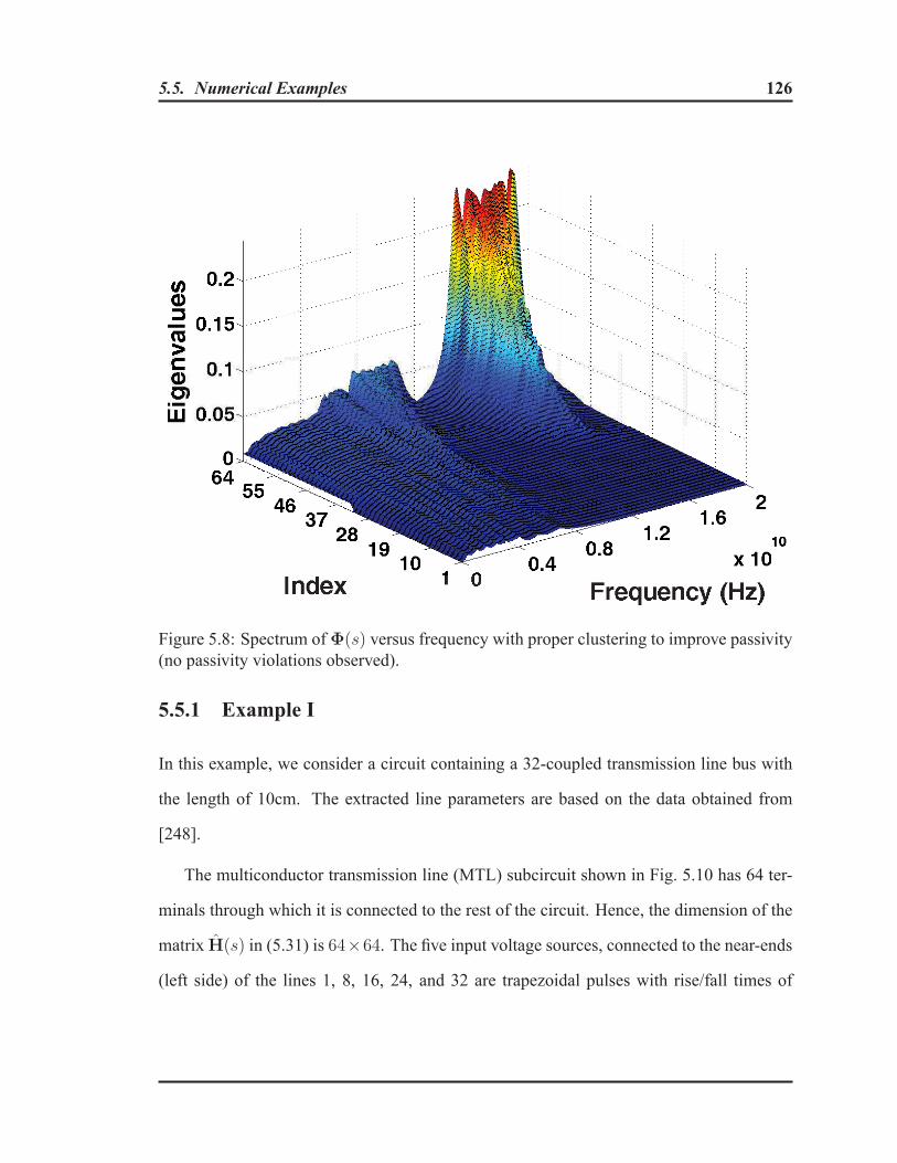
5.5. Numerical Examples 126
Figure 5.8: Spectrum ofΦ(s) versus frequency with proper clustering to improve passivity(no passivity violations observed).
5.5.1 Example I
In this example, we consider a circuit containing a 32-coupled transmission line bus with
the length of 10cm. The extracted line parameters are based on the data obtained from
[248].
The multiconductor transmission line (MTL) subcircuit shown in Fig. 5.10 has 64 ter-
minals through which it is connected to the rest of the circuit. Hence, the dimension of the
matrix H(s) in (5.31) is 64×64. The five input voltage sources, connected to the near-ends
(left side) of the lines 1, 8, 16, 24, and 32 are trapezoidal pulses with rise/fall times of
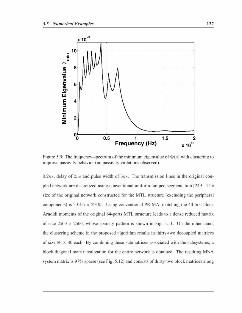
5.5. Numerical Examples 127
0 0.5 1 1.5 2
x 1010
0
2
4
6
8
10
x 10−3
Frequency (Hz)
Min
imu
m E
igen
valu
e λ
min
Figure 5.9: The frequency-spectrum of the minimum eigenvalue ofΦ(s) with clustering toimprove passivity behavior (no passivity violations observed).
0.2ns, delay of 2ns and pulse width of 5ns. The transmission lines in the original cou-
pled network are discretized using conventional uniform lumped segmentation [249]. The
size of the original network constructed for the MTL structure (excluding the peripheral
components) is 29195 × 29195. Using conventional PRIMA, matching the 40 first block
Arnoldi moments of the original 64-ports MTL structure leads to a dense reduced matrix
of size 2560 × 2560, whose sparsity pattern is shown in Fig. 5.11. On the other hand,
the clustering scheme in the proposed algorithm results in thirty-two decoupled matrices
of size 80 × 80 each. By combining these submatrices associated with the subsystems, a
block diagonal matrix realization for the entire network is obtained. The resulting MNA
system matrix is 97% sparse (see Fig. 5.12) and consists of thirty-two block matrices along

5.5. Numerical Examples 128
Figure 5.10: 32 conductor coupled transmission line network with terminations consideredin the example.
the diagonal each of size 80 × 80. This represents significant sparsity advantage com-
pared to using the conventional PRIMA algorithm. To demonstrate the accuracy of the
proposed method, Figures 5.13–5.15 show sample comparisons of time-domain responses.
In the graphs, the time-domain results obtained from applying the proposed method are
compared to the responses from the original network as well as the conventional PRIMA
reduced model. As seen from the plots, all these responses are in excellent agreement.
Table 5.1 compares the CPU time expense for the transient simulation of the original sys-
tem versus the proposed and conventional PRIMA based reduced macromodels. As the
table depicts, applying a conventional MOR technique to this multiport system leads to a
macromodel which is prohibitively expensive; even when compared to the unreduced cir-
cuit. In contrast, using the proposed algorithm, a speed-up of 15.5 compared to PRIMA
was achieved. It was also observed that the speed-up ratio increases with increasing the
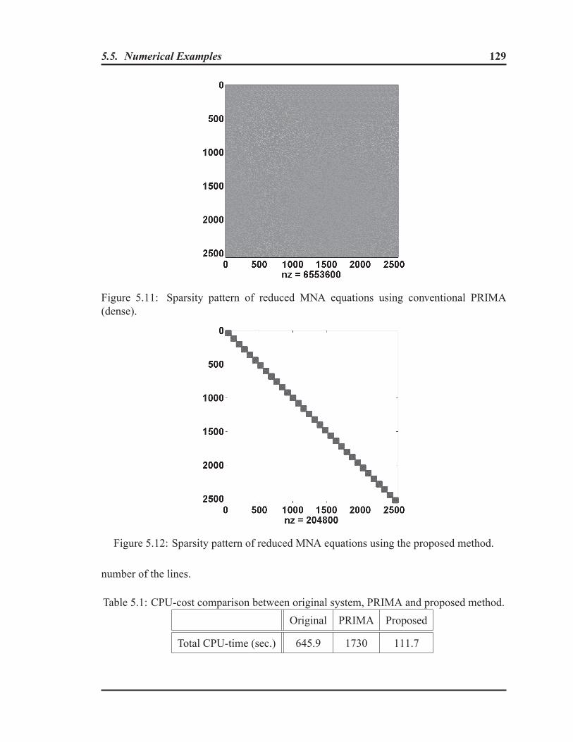
5.5. Numerical Examples 129
Figure 5.11: Sparsity pattern of reduced MNA equations using conventional PRIMA(dense).
Figure 5.12: Sparsity pattern of reduced MNA equations using the proposed method.
number of the lines.
Table 5.1: CPU-cost comparison between original system, PRIMA and proposed method.Original PRIMA Proposed
Total CPU-time (sec.) 645.9 1730 111.7

5.5. Numerical Examples 130
0 0.5 1 1.5 2 2.5
x 10−8
−0.1
−0.05
0
0.05
0.1
0.15
time (sec.)
Vo
ut (
Vo
lt)
OriginalPRIMAProposed
Figure 5.13: Transient responses at victim line near-end of line#2.
5.5.2 Example II
The idea of passivity preservation using the proposed flexible clustering is further inves-
tigated in this example. For the purpose of illustration, we consider an interconnection
structure consisting of nine coupled lines of length d = 2.54 cm (see Fig 5.16). The RLGC
parameters of the lines were calculated using the field solver in HSPICE [250].
First, the interconnect structure was clustered into nine subsystems with one active
line in each as shown in Fig. 5.17. The minimum (smallest) eigenvalue of Hermitian ma-
trix Φ(s) in (5.30c) as function of frequency (λmin (sj) =2N
mini=1
λi (Φ(sj)) ) is shown in
Fig. 5.18 which depicts the presence of negative eigenvalues indicating passivity violation.
This is also illustrated in Fig. 5.19 which shows all the negative eigenvalues ofΦ(s) within
the frequency spectrum of interest. Following the proposed approach, the interconnect
structure was clustered into three subnetworks each including three active lines as shown
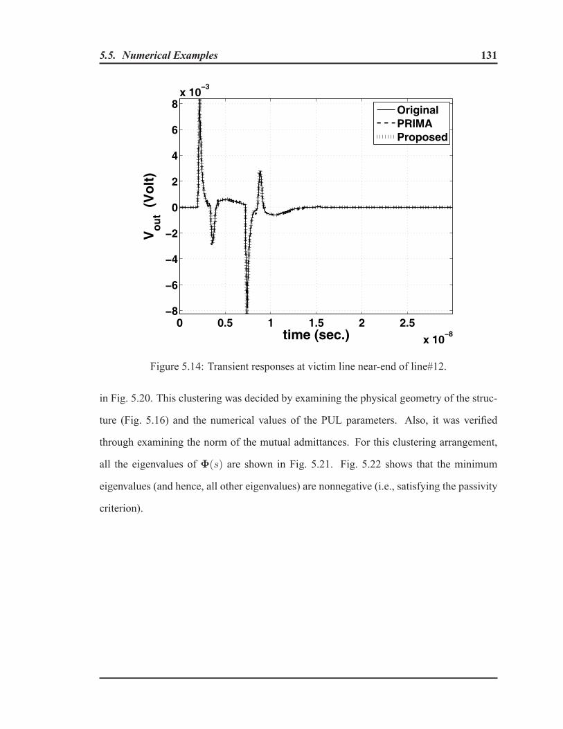
5.5. Numerical Examples 131
0 0.5 1 1.5 2 2.5
x 10−8
−8
−6
−4
−2
0
2
4
6
8x 10
−3
time (sec.)
Vo
ut (
Vo
lt)
OriginalPRIMAProposed
Figure 5.14: Transient responses at victim line near-end of line#12.
in Fig. 5.20. This clustering was decided by examining the physical geometry of the struc-
ture (Fig. 5.16) and the numerical values of the PUL parameters. Also, it was verified
through examining the norm of the mutual admittances. For this clustering arrangement,
all the eigenvalues of Φ(s) are shown in Fig. 5.21. Fig. 5.22 shows that the minimum
eigenvalues (and hence, all other eigenvalues) are nonnegative (i.e., satisfying the passivity
criterion).

5.5. Numerical Examples 132
0 0.5 1 1.5 2 2.5
x 10−8
−0.2
−0.1
0
0.1
0.2
0.3
time (sec.)
Vo
ut (
Vo
lt)
OriginalPRIMAProposed
Figure 5.15: Transient responses at victim line far-end of line#31.
t
h4
S1 S2
Wt
h3
h2
h1
#2
#3
#1
#4
#6
#5
#7
#8
#9
r 4.5ε =
1
2
4
3
h 50 m
h 25 m
h 17
h
0 m
=
= μ
= μ
= μ
Aluminum:
t 5 m
W 25 m
= μ
= μ
1
2
S 25 m
S 50 m
= μ
= μ
Figure 5.16: Cross sectional geometry (Example 2).

5.5. Numerical Examples 133
Sub#1 Sub#2 Sub#3
#5 #6
#7
#4
#8 #9
Figure 5.17: Interconnect structure with nine clusters (Example 2).
0.5 1 1.5 2
x 1010
−2
−1
0
1
2
3
x 10−3
Frequency (Hz)
Min
imu
m E
igen
val λ
min
Figure 5.18: Minimum eigenvalue of Φ(s) while using 9 clusters (each cluster with ninelines while one of them acting as an active line).
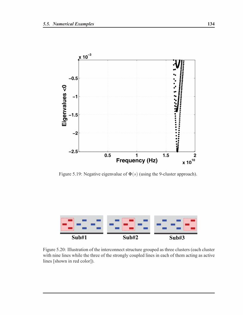
5.5. Numerical Examples 134
0.5 1 1.5 2
x 1010
−2.5
−2
−1.5
−1
−0.5
x 10−3
Frequency (Hz)
Eig
enva
lues
<0
Figure 5.19: Negative eigenvalue of Φ(s) (using the 9-cluster approach).
Sub#1 Sub#2 Sub#3
Figure 5.20: Illustration of the interconnect structure grouped as three clusters (each clusterwith nine lines while the three of the strongly coupled lines in each of them acting as activelines [shown in red color]).

5.5. Numerical Examples 135
Figure 5.21: Eigenvalue ofΦ(s) (using 3 clusters based on the proposed flexible clusteringapproach).
0.5 1 1.5 2
x 1010
0
1
2
3
4
5
6
x 10−4
Frequency (Hz)
Min
imu
m E
igen
val λ
min
Figure 5.22: Minimum eigenvalues ofΦ(s) (using 3 clusters based on the proposed flexibleclustering approach).

Chapter 6
Optimum Order Estimation of Reduced Linear
Macromodels
In Chapter 3, some of the well-known linear model reduction methods were reviewed.
Also, it was stated that, presently, a rich body of literature is available covering the linear
MOR techniques. However, for all of these methods, the selection of order is an important
issue. This chapter explains the details of a novel algorithm for optimal-order determination
for the reduced linear macromodels.
6.1 Introduction
An important and practical common problem in prominently used order-reduction tech-
niques is that of “selection of order“ for the reduced model. The proper choice of order
for a macromodel based approximation is important in terms of achieving the pre-defined
accuracy, while not over-estimating the order, which otherwise can lead to inefficient tran-
sient simulations. This (an optimum order) becomes even more important, if the reduced
macromodel is going to be used repeatedly as part of a larger simulation task such as in
136

6.2. Development of the Proposed Algorithm 137
the case of statistical analysis, optimization, design centering, etc. In this case, the unnec-
essary computational cost during repetitive simulations/optimization due to overestimating
the order of the reduced-model can significantly exceed the computational cost of opti-
mally pre-estimating the order. Current techniques for predicting an optimum order for an
approximation a-priori is generally heuristic in nature.
This chapter presents a novel algorithm to obtain an optimally minimum order for a
reduced model under consideration. The proposed methodology is based on the idea of
monitoring the behavior of the projected trajectory in the reduced space [251, 251]. To
serve this purpose, a mathematical algorithm is devised to observe the behavior of near
neighboring points, lying on the projected trajectory, when increasing the dimension of
a reduced-space. The order is determined such that the projected trajectory is unfolded
properly in the reduced space, while monitoring the count of the ”False Nearest Neighbor
(FNN)” points on the projected trajectory. The reduced model in this optimally reduced
subspace preserves the major dynamical properties of the original system.
6.2 Development of the Proposed Algorithm
6.2.1 Preliminaries
A set of differential algebraic equations can be used to represent the dynamical behavior of
the system states [2, 21–23]. For electrical networks these equations are directly obtained
using the modified nodal analysis (MNA) matrix formulation [37–39,167] in the form:
Cd
dtx(t) + Gx(t) = Bu(t) (6.1)
i(t) = Lx(t) , (6.2)

6.2. Development of the Proposed Algorithm 138
whereC andG ∈ Rn×n are susceptance and conductance matrices, respectively, x(t) ∈ R
n
denotes the vector of MNA variables (the nodal voltages and some branch currents) of the
circuit. B and L represent the input and output matrices, respectively.
The key idea in subspace projection-based model order reduction techniques is to
project the original n-dimensional state space to a m-th order (e.g.: Krylov) subspaces,
where practically m � n. This reduction process requires creation of a projection oper-
ator Q = [q1, q2, . . . ,qm] ∈ Rn×m such that the trajectory in the original space can be
properly projected to a reduced subspace as z(t) � QTx(t). As a result, a linear system
which is of much smaller order is obtained by a variable change as x = Qz [64, 89, 90].
The objective of the proposed method is to determine the optimum dimension for the
reduced subspace while preserving desired accuracy. To serve this purpose, the “false
nearest neighbors (FNN)” concept [252–255] is adopted. From a geometrical perspective,
the variables set {xi(t) : for i = 1, 2, . . . , n} is used as a coordinate system to definean n-dimensional space. Therefore, the response at each time instant tj , represented by
x(tj) = {x1(tj), x2(tj), . . . , xn(tj)} (tj ∈ Λt), defines a point in this response space.
Consider the illustrative Fig. 6.1; starting from a given initial condition x(t0), as the cir-
cuit’s response evolves with time, the point moving through the response space traces out
a curve. Mathematically, the solution curve is a real-valued continuously-differentiable
function (taken to be Cn) [22] from an open interval Λt ⊂ R+ into the response space
⊆ Rn. Such a curve as a flow of the states for all subsequent time is the key notion in the
description of the behavior of dynamical circuits. We consider this trajectory curve whose
definition is given below as a geometric model to study the dynamic behavior of the circuit.
Definition 6.1. A time-parameterized path in the multidimensional response space of a
system, defined by x(t) for t ≥ t0 is referred to as trajectory (curve) of the system.
Using a projection operator Qn×m, a reduced subspace Rm is defined with coordinates

6.2. Development of the Proposed Algorithm 139
Figure 6.1: Any state corresponding to a certain time instant can be represented by a point(e.g. A, N, E and F) on the trajectory curve (T) in the variable space.
that are linear combinations of the original coordinates; i.e. zi(t) =n∑
j=1
qji xj(t), for
i = 1, 2 . . . m, wherem << n. An image of the trajectory curve in the low dimensional
subspace is obtained through the point-wise projection of the original trajectory onto the
target subspace as
z(·) = QT x(·) . (6.3)
In such a projection from the original n-dimensional space to its subspace QT x : Rn �→
Rm, the trajectory curve is contracted to reside in the reduced subspace (cf. lemma 6.1).
It is to be noted that, the application of the proposed techniques is not limited to a
specific projection based model order reduction and the projection operators from any of
the projection based methods such as: Krylov-subpace methods [82–85, 90, 91], TBR [88,
104,112], and POD [87,127,210,256] can be used.
The key idea in the proposed optimal order estimation algorithm is to topologically
observe the behavior of near neighboring points, that are lying on the projected trajectory
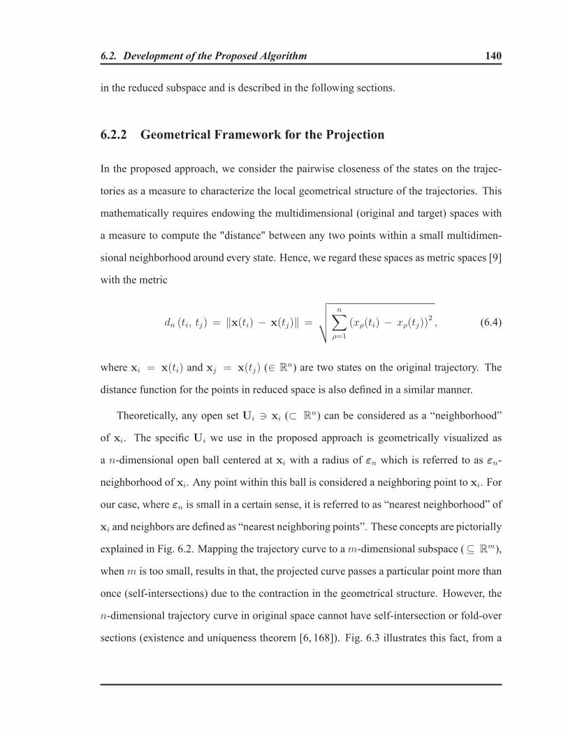
6.2. Development of the Proposed Algorithm 140
in the reduced subspace and is described in the following sections.
6.2.2 Geometrical Framework for the Projection
In the proposed approach, we consider the pairwise closeness of the states on the trajec-
tories as a measure to characterize the local geometrical structure of the trajectories. This
mathematically requires endowing the multidimensional (original and target) spaces with
a measure to compute the "distance" between any two points within a small multidimen-
sional neighborhood around every state. Hence, we regard these spaces as metric spaces [9]
with the metric
dn (ti, tj) = ‖x(ti) − x(tj)‖ =
√√√√ n∑ρ=1
(xρ(ti) − xρ(tj))2 , (6.4)
where xi = x(ti) and xj = x(tj) (∈ Rn) are two states on the original trajectory. The
distance function for the points in reduced space is also defined in a similar manner.
Theoretically, any open set Ui � xi (⊂ Rn) can be considered as a “neighborhood”
of xi. The specific Ui we use in the proposed approach is geometrically visualized as
a n-dimensional open ball centered at xi with a radius of εn which is referred to as εn-
neighborhood of xi. Any point within this ball is considered a neighboring point to xi. For
our case, where εn is small in a certain sense, it is referred to as “nearest neighborhood” of
xi and neighbors are defined as “nearest neighboring points”. These concepts are pictorially
explained in Fig. 6.2. Mapping the trajectory curve to am-dimensional subspace (⊆ Rm),
whenm is too small, results in that, the projected curve passes a particular point more than
once (self-intersections) due to the contraction in the geometrical structure. However, the
n-dimensional trajectory curve in original space cannot have self-intersection or fold-over
sections (existence and uniqueness theorem [6, 168]). Fig. 6.3 illustrates this fact, from a

6.2. Development of the Proposed Algorithm 141
Figure 6.2: Illustration of a multidimensional adjacency ball centered at x(ti), accommo-dating its four nearest neighboring points.
geometrical perspective. It depicts a self-intersection point (A and E) in the projected curve
T, while the corresponding original states (A and E in Fig. 6.1) were not even neighbors,
this occurs since the m-dimensional subspace is too small that the projected curve to be
safely accommodated without over-contracting it. In such conditions, not all points that
lie close to one another (e.g. A, F and E) are neighbors because of the original dynamics.
There is a new neighbor point (e.g. F) on the projected trajectory that is close to a candidate
point (A) solely because we are viewing the path T in a dimension that is too small. In
Fig. 6.4, the neighborhood geometry of the reference point x(ti) in the state space is shown
together with its projection z(ti) and nearest neighbors in the m-dimensional target space.
Two neighboring points z(ti) and z(tk) on the projected path are the images of x(ti) and
x(tk), respectively; while they are not neighbors in the original space. Considering the
aforementioned concepts, the following definitions are formalized.
Definition 6.2. The points z(ti) and z(tk) which are neighbors in the reduced space are

6.2. Development of the Proposed Algorithm 142
Figure 6.3: Illustration of false nearest neighbor (FNN), where T is the projection of T inFig. 1.
defined as “false neighbors“ if x(ti) and x(tk) are not neighbors in the original state space.
Definition 6.3. The neighboring points on the projected trajectory z(ti) and z(tj) are “true
neighbors“ when x(ti) and x(tk) are also neighbors in the original state space.
6.2.3 Neighborhood Preserving Property
In this section, it will be shown that in a projection to a subspace with a sufficient order,
the projected trajectory curve inherits the same neighborhood structure of the original tra-
jectory. This implies that, (a) the original nearest neighboring points remain neighbors in
such a projection, (b) the near neighbors in that reduced subspace are true neighbors.

6.2. Development of the Proposed Algorithm 143
Figure 6.4: Illustration of the neighborhood structure of the state xi and its projection zi inthe state space and reduced space, respectively.
Lemma 6.1. Contraction Property: In projection using an orthogonal matrix Qn×m
(m << n), the inner points of εn-neighborhood of any point on the original (n-
dimensional) trajectory are preserved as inner points of εm-neighborhood in (m-
dimensional) reduced subspace, where εm < εn.
Proof. Let x(ti) be any arbitrarily selected state on the original trajectory and x(tj) be a
neighboring state lying in the εn-neighborhood of x(ti). Also, let z(ti) and z(tj) respec-
tively, be the images of x(ti) and x(tj) in a reduced subspace of order m. The Euclidean
distance between these points is
dm (ti, tj) = ‖z(ti)− z(tj)‖ =∥∥QT x(ti)−QT x(tj)
∥∥=
∥∥QT (x(ti)− x(tj) )∥∥ ≤ ∥∥QT
∥∥ ‖x(ti) − x(tj)‖ . (6.5)

6.2. Development of the Proposed Algorithm 144
Using the following properties of the matrix 2-norm [117]
‖QT‖ = ‖Q‖ , (6.6a)
‖Q‖ =√
λmax (QT Q) = δmax(Q) , (6.6b)
and for any orthogonal matrixQ
δmax(Q) = 1 , (6.6c)
where λmax and δmax denote the largest eigenvalue and the largest singular value, respec-
tively. Considering the above properties (6.6a) - (6.6c) and using (6.5) we get
dm (ti, tj) ≤ ‖x(ti) − x(tj)‖ . (6.7)
x(tj) being in the open εn-neighborhood of x(ti), we have ‖x(ti) − x(tj)‖ < εn. Hence,
from (6.7),
‖z(ti) − z(tj)‖ < ‖x(ti) − x(tj)‖ < εn . (6.8)
Next, consider the surface of εm-neighborhood ball centered at any arbitrary point z(ti) ∈T, defined as
{z(t) | z(t) ∈ Rm & dm (ti, t) = εm } . (6.9)
Using (6.8), it is straightforward to show that,
εm < εn . (6.10)
This concludes the proof of the contraction property. �
Lemma 6.2. The accuracy for the macromodel is ensured if and only if all the nearest
neighboring points on the projected trajectory are true neighbors.

6.2. Development of the Proposed Algorithm 145
Proof. First, assuming a sufficient order for the reduced macromodel that can ensure an ad-
equate accuracy, we prove that any two near neighboring points on the projected trajectory
T are true neighbors. Let�
T ={
�z(t) : for t ∈ Λt
}denote the trajectory curve obtained
from a reduced model. Consider z(tj) to be a point in the εm-neighborhood of any arbitrary
z(ti) (j �= i) on the projected trajectory T, we have
dm (ti, tj) = ‖z(ti) − z(tj)‖ < εm , (6.11)
where εm is a small neighborhood radius. Equation (6.11) can be equivalently rewritten as
‖z(ti) − z(tj)‖ =∥∥QTx(ti) − QTx(tj)
∥∥ < εm . (6.12)
From the direct solution of the reduced system �z(t), the approximated responses xa(ti) and
xa(tj) are obtained as
xa(ti) = Q�z(ti) ,
xa(tj) = Q�z(tj) . (6.13)
Let the error vectors between the actual and approximated responses at time instants ti and
tj be denoted as ζi and ζj (∈ Rn), respectively,
x(ti) − xa(ti) = ζi ,
x(tj) − xa(tj) = ζj . (6.14)
Assuming that the orderm0 is sufficient to ensure accuracy of the reduced model,
‖ζi‖ = ‖x(ti)− xa(ti)‖ < ξer,

6.2. Development of the Proposed Algorithm 146
∥∥ζj
∥∥ = ‖x(tj)− xa(tj)‖ < ξer, (6.15)
where ξeris a small positive value. By substituting x(ti) and x(tj) from (6.13) and (6.14)
in (6.12), we get
∥∥QTx(ti) − QTx(tj)∥∥ =
∥∥QT(Q
�z(ti) + ζi
) − QT(Q
�z(tj) + ζj
)∥∥ =∥∥(�z(ti) − �
z(tj)) − QT
(ζj − ζi
)∥∥ < εm . (6.16)
The inverse triangle inequality [75] holds for any two vectorsV1, V2 ∈ Rm holds as
‖V1‖ − ‖V2‖ ≤ ‖V1 −V2‖ . (6.17)
Using this property, from (6.16) we get
‖�z(ti) − �
z(tj)‖ − ‖QT(ζj − ζi
) ‖ ≤∥∥(�z(ti) − �
z(tj)) − QT
(ζj − ζi
)∥∥ < εm . (6.18)
Applying (6.6) on (6.18), we get
‖�z(ti) − �
z(tj)‖ < εm + ‖ζj − ζi‖ < εm + ‖ζi‖ + ‖ζj‖ < εm + 2ξer. (6.19)
This proves that �z(ti) and�z(ti) to be neighboring points on the solution trajectory obtained
from the reduced macromodel. Multiplying both sides of (6.19) by ‖Q‖ = 1 in (6.6), we
get
‖Q‖ ∥∥�z(ti) − �
z(tj)∥∥ < εm + 2ξ
er. (6.20)

6.2. Development of the Proposed Algorithm 147
It is ∥∥Q (�z(ti) − �
z(tj))∥∥ ≤ ‖Q‖ ∥∥�
z(ti) − �z(tj)
∥∥ < εm + 2ξer. (6.21)
Combining (6.13) and (6.14) with (6.21) results in
∥∥x(ti) + ζi − x(tj) − ζj
∥∥ < εm + 2ξer
(6.22)
and
‖x(ti) − x(tj)‖ < εm + 4ξer. (6.23)
Hence, xj falls within a close neighborhood of xi. This verifies that x(ti) and x(tj) are
neighboring points on the original trajectory and indicates z(ti) and z(tj) as true neighbors.
Second, we prove that, having all the nearest neighbors on the projected trajectory as
true neighbors is a sufficient condition, to guarantee the accuracy of the reduced macro-
model. For this, let z(tj) be a neighboring point to an arbitrarily selected point on the
projected trajectory z(ti) (j �= i). Being a true near neighbor, the corresponding state x(tj)
lies within a small neighborhood ball of x(ti). This requires that the right hand side of the
equation in (6.23) to be upper bounded to a small value, as
‖x(ti)− x(tj)‖ < εm + 4ξer
≤ εn . (6.24)
From (6.24),
ξer
≤ εn − εm
4, (6.25)
where both neighborhood radii εn > εm > 0 are small. According to (6.25), the small
values of εn and εm guarantee the accuracy of the macromodel by upper-bounding the
errors to a small value at all time instants throughout the projected trajectory. �
Lemma 6.2 establishes that, when the reduced space is of a sufficient dimensionality

6.2. Development of the Proposed Algorithm 148
such that no false neighbors are present in the reduced space, a sufficient level of accuracy
is ensured for the model. These facts form the underlying idea for the proposed method
which is mainly based on successively reversing the trajectory folding process.
6.2.4 Unfolding the Projected Trajectory
Starting from a low-dimensional space, the order of the reduced space is consecutively
increased. In each step, the projected trajectory is expanded into higher dimensions. Con-
sequently, some neighboring points move far apart and reveal themselves as false nearest
neighbors. This can be visualized as gradually unfolding the sections that have been folded
over. The count of false nearest neighbors can be utilized to monitor this unfolding process.
Ultimately, at some order (e.g. m0), the count of false nearest neighbors drops to zero, such
that, further increasing the order does not help the unfolding, and hence does not lead to
revealing any new false nearest neighbors. Only then the points which are true neighbors
on the original trajectory will stay neighbors on the projected trajectory in reduced space.
This fact is illustrated in Fig. 6.5, where the changes of two nearest-neighbors (A and B)
in a transition from order m to m + 1 is visualized. It shows a trajectory embedded in a
subspace with insufficient order (m < m0). By adding the (m+ 1)-th dimension, these
two points move apart to their new locations A and B, respectively. Their distance in the
m dimension space; AB = dm(i, j) was changed to AB = dm+1(i, j) in the m + 1 di-
mensional subspace. In the unfolding process, such large change in separation between A
and B indicates B as a false neighbor of A inm dimension. From Fig. 6.5 we have,
d2m+1(i, j) = d2m(i, j) + (zm+1(ti) − zm+1(tj))2 . (6.26)

6.2. Development of the Proposed Algorithm 149
Figure 6.5: Displacement between two false nearest neighbors in the unfolding process.
In the proposed method, the component of the displacement vector between two neighbors
on the new axis
Δzm+1(i, j) = |zm+1(ti)− zm+1(tj)| , (6.27)
is used as a measure to monitor the behavior of the neighboring points in the unfolding
process. IfΔzm+1(i, j) is not small compared to their Euclidean distance dm(i, j), they are
false neighbors. This comparison is performed by checking the following ratio [253,257]
Rij =
[d2m+1(i, j)− d2m(i, j)
d2m(i, j)
]1/2=
|zm+1(ti) − zm+1(tj)|dm(i, j)
=Δzm+1(i, j)
dm(i, j). (6.28)
This central idea is summarized in the following corollary.
Corollary 6.1. The order m0 is an optimally minimum reduction order if increasing the
order of the reduced subspace to m1, where m1 > m0 does not reveal any false nearest
neighboring points on the reduced trajectory.

6.3. Computational Steps of the Proposed Algorithm 150
6.3 Computational Steps of the Proposed Algorithm
The steps of the proposed algorithm are summarized as follows. For the sake of simplicity
in the notation, hereafter, we drop “t” in the equations (e.g. z(ti) is referred to as z(i)).
(1) The proposed algorithm uses the time series data from the projected trajectory
z(·) ∈ Rm×N,
z(·) = {z(i) ∈ R
m×1 | z(i) = QT x(i), for i = 1, . . . ,N}. (6.29)
This requires one-time transient simulation of the circuit with any arbitrary inputs with a
wide frequency spectrum up to the maximum frequency of interest to obtain the response
x(·). It is to be noted that, the typical goal of linear model reduction is to accuratelyrepresent a particular system output up to a certain maximum frequency as dependent on
the specific application. Therefore, it is essential that the spectrum of the excitation signals
adequately cover the frequency range of interest.
The projection matrix Q is formed with a small initial number (m) of orthonormal basis,
and the time series data z(·) is obtained using (6.3).
(2) A set of close pointsΠi to each point on the projected trajectory z(i) is found using
the following check:
dms(i, j) < R, for j = 1 , · · · , N and j �= i , (6.30)
where R is a search radius.
In general, any choice ofR which leads toΠi containing a few close points is adequate. An
unnecessary large search radius, leads to a (unnecessary) large number of the neighbors.
This does not improve the result, but may takes unnecessary CPU time and slow down the
algorithm.

6.3. Computational Steps of the Proposed Algorithm 151
Efficient neighborhood searching algorithms have been extensively studied in computa-
tional geometry and image processing [258–260]. However, due to the relatively small size
of the data set (m × N ) in this step of the proposed method, a simple and straightforward
search algorithm as outlined in “Algorithm-5” is adequate.
(3) Next, the number of orthogonal basis is increased from m to m + 1 and the new di-
mension of the time-series data for the projected trajectory is computed
z(m+1)(·) = qT(m+1)x(·) . (6.31)
(4) All the close points z(j) ∈ Πi to z(i) i = 1, . . . , N , that satisfies the following ratio
(6.28) test are marked as false neighbors
Rij =Δzm+1(i, j)
dm(i, j)> ρt , (6.32)
where ρt is a pre-specified threshold value.
This FNN search process is summarized in “Algorithm-6”.
(5) By repeating the steps (2)-(4), the projected trajectory is unfolded into higher di-
mensions. Ultimately, at some order m0, the count of false nearest neighbors in step (4)
drops to zero, such that, further increasing the order does not lead to revealing any new false
nearest neighbors. According to Corollary 6.1, m0 is designated as the optimum minimal
dimension for the reduced subspace.
The above computational steps are summarized in the pseudo codes depicted in
"Algorithm-5", "Algorithm-6" and "Algorithm-7".
The following points are also worth mentioning:
1) The initial search for close neighbors in “Algorithm-5” is performed only once on the
N × m time series from the projected trajectory, where m is a small (starting) order and

6.3. Computational Steps of the Proposed Algorithm 152
Algorithm 5: Neighborhood SearchData: z ∈ R
m×N (Data matrix for the projected trajectory)Result: Π (Neighborhood information)
1 I ← {i | 1 ≤ i ≤ N };2 foreach i ∈ I do3 foreach j ∈ I− {i} do4 Find dm(i, j) ;5 if dm(i, j) < R (6.30) then6 Πi ← ( j, dm(i, j) );
Algorithm 6: False Nearest Neighbor (FNN)Data: zm+1 ∈ R
m×1 (new coordination)Result: False nearest neighbor count &Π (updated)
1 foreach i ∈ I (If Πi �= 0) do2 foreach j ∈ Πi do3 Compute Rij from (6.32);4 if Rij > ρt (6.32) then5 False nearest neighbor count + 1;6 Compute dm+1(i, j) from (6.26);7 Πi ← ( j, dm+1(i, j) );
Algorithm 7: Proposed Order Estimation AlgorithmData: x ∈ R
n×N (Data matrix from trajectory)Result: Optimally minimum reduction order (m0)
1 m ← An arbitrary (small-starting) order;2 Qn×m ← Projection matrix;3 Find projected trajectory z(·) from (6.3) ;4 Π ← From Algorithm-5;
5 while False nearest neighbor count > 0 do6 m ← m + 1;7 Find qm+1 ;8 Find zm+1 from (6.31);9 False nearest neighbor count, Π ← From Algorithm-6;10 Optimally minimum reduction order (m0) ←m
6.4. Numerical Examples 153
N is the number of time points (generally, in the range of a few hundreds). Finding all
neighbors in a set of N vectors of size m can be performed in O (N log(m)) or O (N)
under mild assumptions [260,261].
2) The computational complexity of the false nearest neighbors (FNN) search in
“Algorithm-6” is O (Nn). In addition, the FNN algorithm is suitable for parallel imple-
mentation leading to additional reduction in the computational cost [262].
3) The proposed method does not require the formulation or simulation of the reduced
macromodel.
4) Increasing the number of orthogonal basis from m to m + 1 keeps the initial m basis
unchanged and thus requires the computation of only one new vector.
6.4 Numerical Examples
In this section, numerical results are presented to demonstrate the validity, performance and
accuracy of the proposed methodology. It is to be noted that the proposed method is not
limited to any specific projection method. For the purpose of illustration, the block Krylov
subspace based projection method [64, 90] is used in the following numerical examples.
6.4.1 Example I
In this example, the transmission line shown in Fig. 6.6 is considered. The per-unit-length
parameters are C = 1.29 pF/cm, L = 3.361nH/cm and R = 5.421Ω/cm. The transmis-
sion line is discretized using conventional lumped segmentation [249] to the form of 1500
lumped RLGC π-sections in cascade. The order of the subcircuit (excluding terminations)
is 4500.
The input excitations at the two ports of the transmission line are set to be Gaussian

6.4. Numerical Examples 154
d = 25 cmRin
Vs
RsLs
Cp GPCp/2 GP/2
RsLs
Cp/2 GP/2Cp GP
Rin
seg.#1 seg.#1500
(a)
(b)
Vs
RL CL
RL CL
L inR =R = 50Ω
LC 1pF=
Figure 6.6: (a) A lossy transmission line as a 2-port network with the terminations;(b) Modeled by 1500 lumped RLGC π-sections in cascade.
voltage pulses with 60dB bandwidth at 5 GHz [263]. The terminal currents define the
output vector.
Applying the proposed method, Fig. 6.7 shows the count of the false nearest neigh-
bors on the projected trajectory, while the dimension of the model is changed from m to
m + 1. Here, the vertical axis in Fig. 6.7 represents the percentage of the total count of
FNN compared to the total count of neighbors. As seen from Fig. 6.7,m ≥ 65 completely
unfolds the projected trajectory with no false neighbors. Hence, according to Corollary-
6.1, m = 66 is selected as the optimum order. The original subcircuit is reduced using the
PRIMA algorithm with order 66. The equations of the reduced model are combined with
the MNA equations of the rest of the circuit [264]. The input voltage source was a trape-
zoidal pulse with rise/fall times of 0.1ns, delay of 1ns and pulse width of 5ns. Comparison
of the simulation results obtained from the original circuit of Fig. 6.6 and from the reduced
circuit are shown in Fig. 6.8–6.9, which show excellent agreement.
To validate thatm = 66 is the the optimum order, the voltage responses at the two ends
of the subcircuit in Fig. 6.6 were recorded. The error in the response obtained from the

6.4. Numerical Examples 155
2 5 8 11 14 17 20 23 26 29 32 35 38 41 44 47 50 53 56 59 62 65 68 71 740
10
20
30
40
50
Dimension
Fal
se N
N (
%)
FNN (%)
Optimum Order
Figure 6.7: The percentage of the false nearest neighbors on the projected trajectory.
reduced circuit is defined as
ek(·) = SOriginal
k (·) − SReduced
k (·) ,
RMS Error =
(1
PNt
P∑k=1
‖ek‖22) 1
2
, (6.33)
where Sk denotes the responses at P outputs of interest and Nt is the number of the time
samples. Fig. 6.10 shows the error as function of the order of the reduced subcircuit.

6.4. Numerical Examples 156
0 0.5 1 1.5
x 10−8
0
0.1
0.2
0.3
0.4
0.5
time (sec.)
Vo
ut (
Vo
lt)
OriginalOrder=66
Figure 6.8: Transient response of the current entering to the far-end of the line when thereduced model is of orderm = 66.
6.4.2 Example II
In this example, we consider a RLC mesh shown in Fig. 6.11. The RLC subcircuit (in
Fig. 6.11) is connected to the rest of the circuit through its 24 ports. The order of the
subcircuit (excluding terminations) is 5800.
As explained for example 2, excitations directly at all the ports of the subnetwork are set
to be Gaussian voltage pulses with 60dB bandwidth at the upper frequency limit of interest.
The terminal currents define the output vector. The proposed method (Sec. 6.2) is applied
to estimate the optimum order for the reduced macromodel for subcircuit. Fig. 6.12 shows
the count of the false nearest neighbors on the projected trajectory, while the dimension
of the model is changed from m to m + 1. Here, the vertical axis in Fig. 6.12 represents
the percentage of the total count of FNN compared to the total count of neighbors. As

6.4. Numerical Examples 157
0 0.5 1 1.5
x 10−8
−0.03
−0.02
−0.01
0
0.01
0.02
0.03
0.04
time (sec.)
I in (
Am
p)
OriginalOrder=66
Figure 6.9: Transient response of the current at the far-end terminal of the line when thereduced model is of orderm = 66.
seen from Fig. 6.12, m ≥ 290 completely unfolds the projected trajectory with no false
neighbors. Hence, according to Corollary-6.1,m = 290 is selected as the optimum order.
The original subcircuit is reduced using the PRIMA algorithm with order 290. The
equations of the reduced model are combined with the MNA equations of the rest of the
circuit. The three input voltage sources, connected to the near-ends (left side) of the hori-
zontal traces 1, 6, and 12 are trapezoidal pulses with rise/fall times of 0.1ns, delay of 1ns
and pulse width of 5ns. Comparison of the simulation results obtained from the original
circuit of Fig. 6.11 and from the reduced circuit are shown in Fig. 6.13–6.14, which show
excellent agreement.
To validate that m = 290 is the the optimum order, Fig. 6.10 shows the error in the
output voltages (6.33) as a function of the order of the reduced subcircuit.
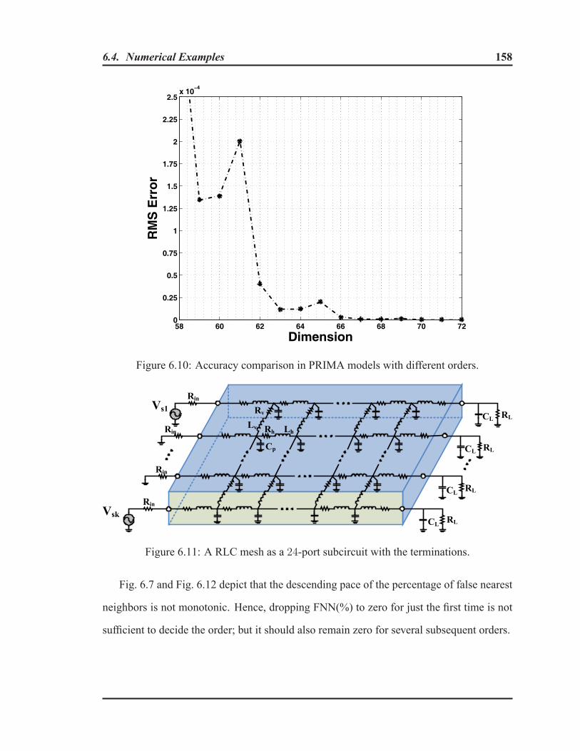
6.4. Numerical Examples 158
58 60 62 64 66 68 70 720
0.25
0.5
0.75
1
1.25
1.5
1.75
2
2.25
2.5x 10
−4
RM
S E
rro
r
Dimension
Figure 6.10: Accuracy comparison in PRIMA models with different orders.
Rh LhLv
Cp
Rv
Rin
Vs1
Rin
Rin
Vsk
Rin
RLCL
RLCL
RLCL
RLCL
Figure 6.11: A RLC mesh as a 24-port subcircuit with the terminations.
Fig. 6.7 and Fig. 6.12 depict that the descending pace of the percentage of false nearest
neighbors is not monotonic. Hence, dropping FNN(%) to zero for just the first time is not
sufficient to decide the order; but it should also remain zero for several subsequent orders.
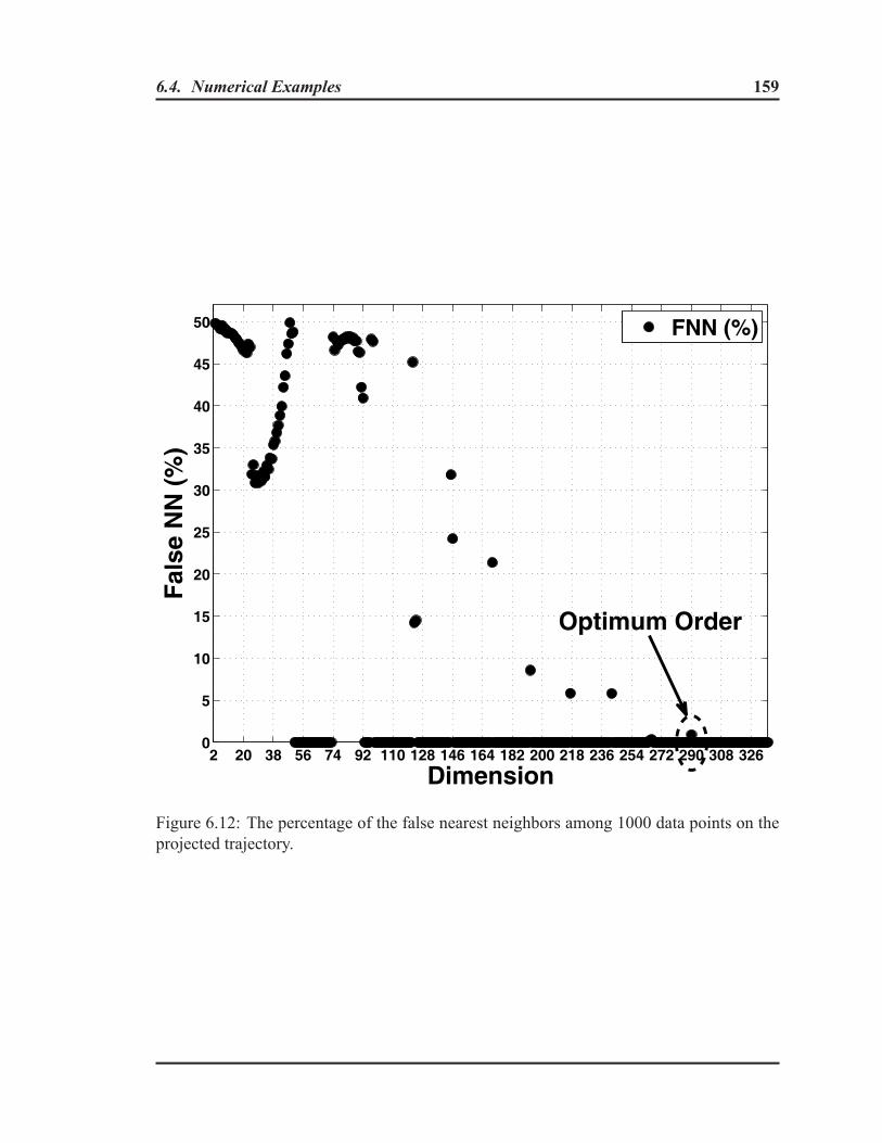
6.4. Numerical Examples 159
2 20 38 56 74 92 110 128 146 164 182 200 218 236 254 272 290 308 3260
5
10
15
20
25
30
35
40
45
50
Dimension
Fal
se N
N (
%)
FNN (%)
Optimum Order
Figure 6.12: The percentage of the false nearest neighbors among 1000 data points on theprojected trajectory.

6.4. Numerical Examples 160
0 0.2 0.4 0.6 0.8 1
x 10−8
0
0.005
0.01
0.015
0.02
0.025
0.03
0.035
0.04
0.045
time (sec.)
I in (
Am
p)
OriginalOrder=290
Figure 6.13: Transient responses at near-end of horizontal trace#1.
0 0.2 0.4 0.6 0.8 1
x 10−8
0
0.05
0.1
0.15
0.2
0.25
0.3
0.35
0.4
0.45
time (sec.)
Vo
ut (
Vo
lt)
OriginalOrder=290
Figure 6.14: Transient responses at near-end of horizontal trace#10.

6.4. Numerical Examples 161
285 286 287 288 289 290 291 292 293 294 295 296 297 298 299 3000
0.5
1
1.5
2
2.5
3
3.5
4
4.5
5x 10
−4
RM
S E
rro
r
Dimension
Figure 6.15: Errors from using the reduced models with different orders in the frequencydomain.
Chapter 7
Optimum Order Determination for Reduced
Nonlinear Macromodels
Chapter 4 presented some of the well-known methods for the reduction of nonlinear sys-
tems such as Taylor series based methods, Trajectory PieceWise Linear (TPWL)-based
methods, Proper Orthogonal Decomposition (POD), and Empirical Balanced Truncation.
An important common problem in these nonlinear order-reduction techniques is the selec-
tion of order for the reduced model. In this chapter, the detail of a novel algorithm for
optimal-order determination for the reduced nonlinear models is presented.
7.1 Introduction
In the prominently used nonlinear order-reduction techniques, “selection of order” is an
important practical issue. The selection of an optimum order is important to achieve a
pre-defined accuracy while not over-estimating the order, which otherwise can lead to inef-
ficient transient simulations and hence, undermine the advantage from applying MOR. The
reduced-order estimation issue for linear circuits has been recently addressed in [251, 265]
and explained in the previous chapter.
162
7.2. Background 163
This chapter presents a novel algorithm to determine an optimally minimum order for a
nonlinear circuit reduction, based on the geometric theory of nonlinear dynamical circuits
(see e.g. [22, 27–30, 166, 266, 267]). The proposed methodology is founded on the idea
of monitoring the local geometrical structure of the projected nonlinear trajectory in the
reduced space [267]. To serve this purpose, a mathematical algorithm is devised to observe
the behavior of near neighboring points, lying on the low-dimensional nonlinear trajectory,
when increasing the dimension of a reduced-space. The order is determined such that the
projected trajectory is unfolded properly in the reduced space, while monitoring the count
of the ”False Nearest Neighbor (FNN)” points on the projected trajectory. The reduced
model in this optimally reduced subspace captures the major dynamical properties of the
original system.
7.2 Background
The general class of systems occurring in a broad range of engineering problems is known
as dynamical systems, whose behavior changes in time according to some deterministic
rules. These rules specify, how a system’s states evolve by time starting from an initial
condition. A set of coupled Differential-Algebraic Equations (DAE) constitutes a mathe-
matical model to characterize their dynamical behavior. Then, mapping from the space of
input signals to the space of output signals is completed by an algebraic equation called
output equation.
7.2.1 Formulation of Nonlinear Circuit Equations
Nonlinear electrical circuits can also be characterized in time-domain by a set of coupled
nonlinear first-order DAE [21–23, 25, 27, 164–166]. In the context of circuit simulation,

7.2. Background 164
these equations are directly obtained from the circuit netlist using the Modified Nodal Anal-
ysis (MNA) matrix formulation [37–39,167] as follows:
Cd
dtx(t) + Gx(t) + f (x(t)) = Bu(t) (7.1)
y(t) = Lx(t) (7.2)
where C andG ∈ Rn×n are susceptance and conductance matrices including the contribu-
tion of linear elements, respectively, x(t) ∈ Rn denotes the vector of MNA variables (the
nodal voltages, some branch currents and electrical charges) of the circuit. f (x) ∈ Rn is a
vector of real-valued functions including the stamps of all nonlinear elements in the circuit.
B and L are the input and output matrices, respectively.
7.2.2 Model Order Reduction of Nonlinear Systems
The basic idea of model order reduction of a circuit is to replace the original system by
an approximated system with a reduced DAE realization of orderm, which is significantly
smaller than the original order n. Model reduction algorithms seek a proper order m for
which the outputs from the reduced system and the original responses are approximately
equal for inputs of interest u(t).
7.2.3 Projection Framework
In any projection based reduction process, an original n-dimensional state space is pro-
jected to to am-th order subspace (m � n). This requires the creation of some projection
operatorsW and Q ∈ Rn×m, whereWT Q = Im×m. Assume that, there exists z(t) ∈ R
q
in a reduced subspace such that it satisfies x(t) = Qz(t). Due to the orthogonality of
the projection matrices (W and Q), z(t) = WT x(t). The differential equations for the

7.2. Background 165
reduced system are obtained through a variable change from (7.1) and (7.2) as
WT d
dtC (Qz(t)) = WTf (Qz(t)) +
(WT B
)u (t) (7.3)
y (t) = (LQ) z(t) (7.4)
The approximate response x(t) is obtained by solving the reduced-order dynamical model
in (7.3) as x(t) = Qz(t). The error between the original state variables and its approxima-
tion is ζ = x−QWTx. For a Galerkin projection scheme, i.e.W = Q.
In the rest of this chapter, we will use the classical POD [210,256] to describe the pro-
posed algorithm for order estimation. However, it should be emphasized that, the proposed
algorithm is not limited to a specific nonlinear model order reduction method and can be
used in conjunction with any of the above mentioned methods.
Using the POD method, for a given representative input u(t), the “time-snapshots” of
the transient response are collected in a data matrix as X = [x(t0), x(t1), . . . , x(tN)] ∈R
n×N . The POD method seeks to find a projection basis Q to accurately approximate
the original response with an approximate representation of data points by minimizing
the overall projection error ‖ζ‖2 =∥∥X−QQTX
∥∥2. The solution to this optimization
problem is obtained by performing singular value decomposition (SVD) on the data matrix
as X = VΣUT [256]. The POD basis for a Galerkin projection is given by the first m
columns inV (∈ Rn×n) asQ = [v1, . . . , vm] ∈ R
n×m.
POD constructs the matrixQ as shown in Algorithm 8.
POD is known as a promising method to provide efficient and accurate transient sim-
ulation (e.g. more accurate than the TPWL [256]). This is for the output responses
corresponding to a family of excitation signals close to the one used to form the POD
basis.
7.3. Order Estimation for Nonlinear Circuit Reduction 166
Algorithm 8: POD procedure for constructingQ of dimensionminput : Original trajectory x(·), reduction order moutput: Projection Matrix Q
1 Access the transient response data matrix,X = [x(t1), x(t2), . . . , x(tN)] ∈ Rn×N ;
2 Perform the SVD ofX: X = VΣUT withV = [v1, . . . , vN ] ∈ R
n×n, Σ ∈ Rn×N andU ∈ R
N×N;3 Truncate the firstm left singular vector to obtain the order reduction projectionmatrix Q = [v1, . . . , vm] (∈ R
n×m);
7.3 Order Estimation for Nonlinear Circuit Reduction
7.3.1 Differential Geometric Concept of Nonlinear Circuits
In this subsection, we define the concepts of the geometric theory of nonlinear dynamical
circuits [22, 27, 29, 30, 166] that are related to this work, in a rather intuitive manner.
Let x(t) = {xi(t) : for i = 1, 2, . . . , n} denote the variables set in the state equa-tion (7.1). The variables set x(t) is used as a coordinates system in an n-dimensional
space, called state space. It is a geometric model for the set of all possible states in the
dynamic (transient) behavior of a nonlinear system for any possible inputs. Consider the
solution of (7.1) for a given input u(t) and an initial condition x0. This solution x(t) would
be a set of time-dependent functions xi(t) (1 ≤ i ≤ n), which are practically obtained
through transient simulation as a set of time-sequenced (time-series) data throughout a cer-
tain time span ti ∈ D = [t0, tmax]. The response at each time instant ti, represented by
x(ti) = [x1(ti), x2(ti), . . . , xn(ti)]T defines a point xi in the multidimensional state space
(xi ∈ S). The locus of states xi in this space for all ti(∈ D ⊂ R+) is a time-parametrized
directional path Φt that starts at the point x(t0) = x0, henceforth this curve is referred to
as the "trajectory" of the system.
These concepts are illustrated in Figures 7.2 and 7.3 for the Chua’s circuit, shown in
Fig. 7.1. The electronic circuit realization and the typical values of the parameters Ga, Gb,
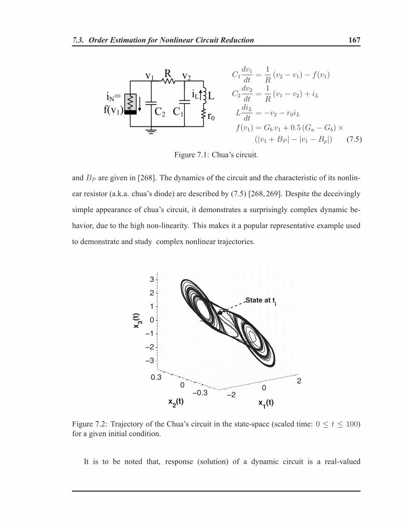
7.3. Order Estimation for Nonlinear Circuit Reduction 167
C1
R
C2 r0
LiLiN=
f(v1)
v1 v2 C1dv1dt
=1
R(v2 − v1)− f(v1)
C2dv2dt
=1
R(v1 − v2) + iL
LdiLdt
= −v2 − r0iL
f(v1) = Gb v1 + 0.5 (Ga −Gb)×(|v1 +BP | − |v1 − Bp|) (7.5)
Figure 7.1: Chua’s circuit.
and BP are given in [268]. The dynamics of the circuit and the characteristic of its nonlin-
ear resistor (a.k.a. chua’s diode) are described by (7.5) [268, 269]. Despite the deceivingly
simple appearance of chua’s circuit, it demonstrates a surprisingly complex dynamic be-
havior, due to the high non-linearity. This makes it a popular representative example used
to demonstrate and study complex nonlinear trajectories.
−20
2
−0.30
0.3
−3
−2
−1
0
1
2
3
x1(t)x
2(t)
x 3(t)
State at ti
Figure 7.2: Trajectory of the Chua’s circuit in the state-space (scaled time: 0 ≤ t ≤ 100)for a given initial condition.
It is to be noted that, response (solution) of a dynamic circuit is a real-valued

7.3. Order Estimation for Nonlinear Circuit Reduction 168
0 20 40 60 80 100−2
0
2
x 1(t)
0 20 40 60 80 100
−0.20
0.2x 2(t
)
0 20 40 60 80 100
−202
t
x 3(t)
ti
ti
ti
Figure 7.3: The time-series plot of the system variables (xi(t)) as coordinates of state space.
continuously-differentiable function [22] from an open interval D(⊂ R+) into the state
space. Under practical assumptions [270], (7.1) is guaranteed to have a unique analytical
solution over any finite time interval, that passes through the initial state at t = t0 [271].
This establishes a certain properties for the geometrical structure of state trajectories, such
as, trajectories (a) do not intersect each other, (b) do not have self-crossing points, and (c) do
not have over-folding sections [6,7,17,168]. Accordingly, state space of a dynamical non-
linear system is considered as a subspace S (⊆ Rn) with a sufficient dimension to embed all
the possible states trajectories of a dynamic system while ensuring the above properties in
(a)-(c). To further elaborate, we consider an inverter circuit as shown in Fig. 7.4-(a), where
the nonlinear dynamics of the inverter gate is described by its behavioral model shown in
Fig. 7.4-(b) as proposed in [272]. For a set of logic pulses (with different timings) at the
input of inverter circuit, the associated responses are plotted in Fig. 7.5. It depicts a ge-
ometrical structure constituted by the family of response trajectories in its 3-dimensional
state space S, termed manifoldM. The manifold of a nonlinear dynamic circuit attracting

7.3. Order Estimation for Nonlinear Circuit Reduction 169
(a)
(b)
Figure 7.4: (a) Digital inverter circuit; (b) The circuit model to characterize the dynamicbehavior of digital inverter at its ports.
its major response trajectories is a bounded region of the state-space (M ⊂ S), wherethese trajectories exist. The n-dimensional manifold that we consider in this work is the
observable state space of the system which is representative for rich dynamical behavior
of a nonlinear system. To contrast the behavior of linear and nonlinear state-space mod-
els, it should be noted that, for linear systems trajectories often (provably) stay close to
a linear subspace (vector space). Whereas, trajectories of a nonlinear system tend to stay
on a nonlinear manifold (curved surface) which is interpreted as a differentiable (smooth)
geometrical structure [22, 27, 273, 274]. If we then join the other ends, we get a Klein bot-
Figure 7.5: A geometric structureM attracting the trajectories of the circuit in Fig.7.4.

7.3. Order Estimation for Nonlinear Circuit Reduction 170
tle, which requires four dimensions to describe it. Fig. 7.6 pictorially exemplify the notion
of differential manifolds by showing, (a) Möbus and (b) Torus as topological subspaces
locally consisting of 2-D patches of Euclidean space, while they are globally 3-D objects
with curved surfaces. For example, we can fold and attach the ends of the paper and get
a Mobius strip, which requires three dimensions to describe it, but locally, the geometry
is still two-dimensional (in the paper). Similarly, nonlinear manifolds which capture the
major system responses are globally curved surfaces and can not be realized as a subspace
(vector space) always sitting inside a fixed Euclidean space, but it looks locally like Eu-
clidean (vector) space. The above idea is roughly outlined in the following definition.
Definition 7.1. An n-dimensional manifoldM is a topological space so thatM is locally
Euclidean of dimension n, i.e. for every x ∈ M, there exist an open neighborhood of x
that is the same as the open n-dimensional sphere in Rn.
In order to compute the distances on the manifold, one needs to equip a distance metric
to the manifold. Considering the locally Euclidean structure of manifold, the distance
between any two states on the trajectory x(ti) and x(tj) when x(tj) falls within a small
multidimensional neighborhood around x(ti) is trustfully measured using the Euclidean
(a) (b)
Figure 7.6: (a) The Möbus strip and (b) Torus are visualizations of 2D manifolds in R3

7.3. Order Estimation for Nonlinear Circuit Reduction 171
norm as
dn (i, j)Δ= ||x(ti)− x(tj)|| =
√√√√ n∑r=1
(xr(ti)− xr(tj))2 (7.6)
For the sake of simplicity in the notation, henceforth , we drop “(t)” in the equations
(e.g. x(ti) is referred to as xi ).
It is also to be noted that, confining the neighboring search to the close adjacency of ev-
ery state allows the intrinsic metric properties of vector space to be locally used. However,
the global distance between two states on the manifold dS (xi, xj) is generally defined
as the length of the shortest trajectory curve connecting them xixj (Geodesic distance).
Accordingly, the results from using (7.6) to measure the distance for far points can be de-
ceivingly inaccurate. In order to study the global properties of a curve, such as Geodesic
distance, the number of times that a curve wraps around a point or convexity properties,
the topological tools are needed. But the further explanation falls beyond the scope of this
work.
The aforementioned facts imply, the trajectory curves possess certain geometric properties
and structure. Properties of curves can be generically classified into "local properties" and
"global properties". Local properties are the properties that hold in a small neighborhood
of a point on a curve.
In this chapter, the parametrized curves (trajectories) is considered as a geometrical model
to study the dynamic behavior of the nonlinear circuits and to develop the proposed or-
der estimation algorithm for nonlinear circuit reduction. We study the local properties
of trajectories namely the neighborhood structure that is the set of the neighbors for each
points.
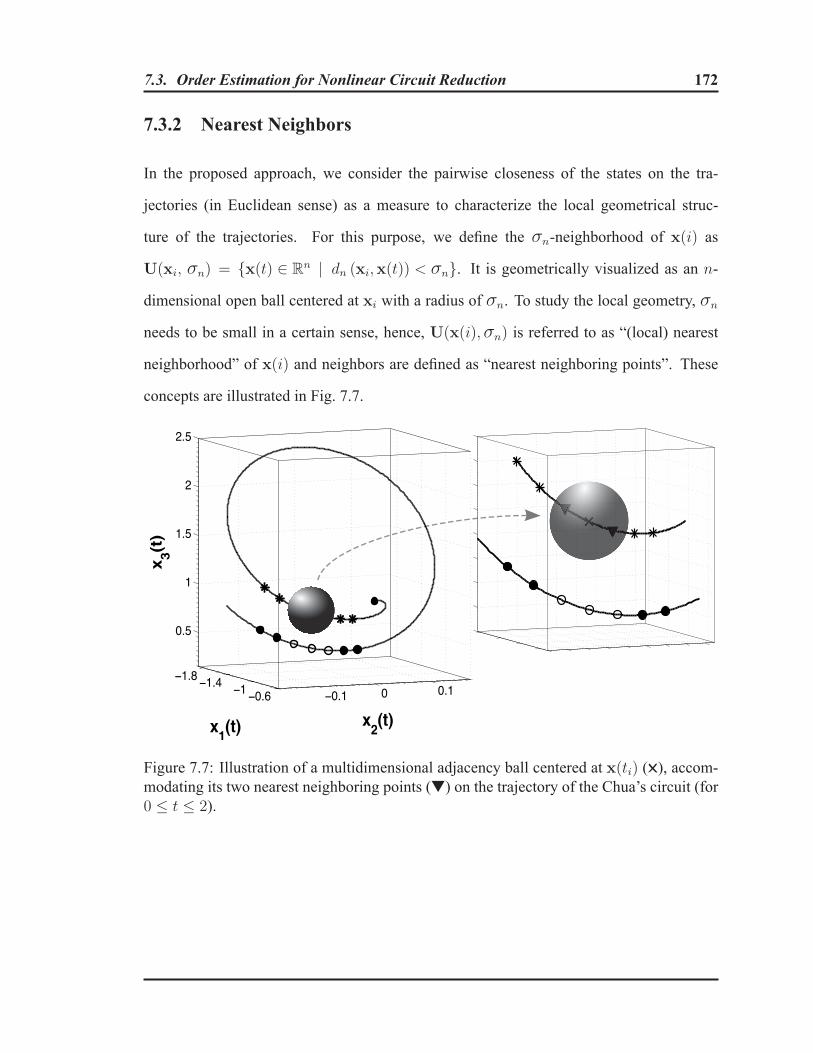
7.3. Order Estimation for Nonlinear Circuit Reduction 172
7.3.2 Nearest Neighbors
In the proposed approach, we consider the pairwise closeness of the states on the tra-
jectories (in Euclidean sense) as a measure to characterize the local geometrical struc-
ture of the trajectories. For this purpose, we define the σn-neighborhood of x(i) as
U(xi, σn) = {x(t) ∈ Rn | dn (xi,x(t)) < σn}. It is geometrically visualized as an n-
dimensional open ball centered at xi with a radius of σn. To study the local geometry, σn
needs to be small in a certain sense, hence, U(x(i), σn) is referred to as “(local) nearest
neighborhood” of x(i) and neighbors are defined as “nearest neighboring points”. These
concepts are illustrated in Fig. 7.7.
1.8 1.4 1 0.6 0.1 0 0.1
0.5
1
1.5
2
2.5
x2(t)x
1(t)
x3(t
)
Figure 7.7: Illustration of a multidimensional adjacency ball centered at x(ti) (✕), accom-modating its two nearest neighboring points (▼) on the trajectory of the Chua’s circuit (for0 ≤ t ≤ 2).
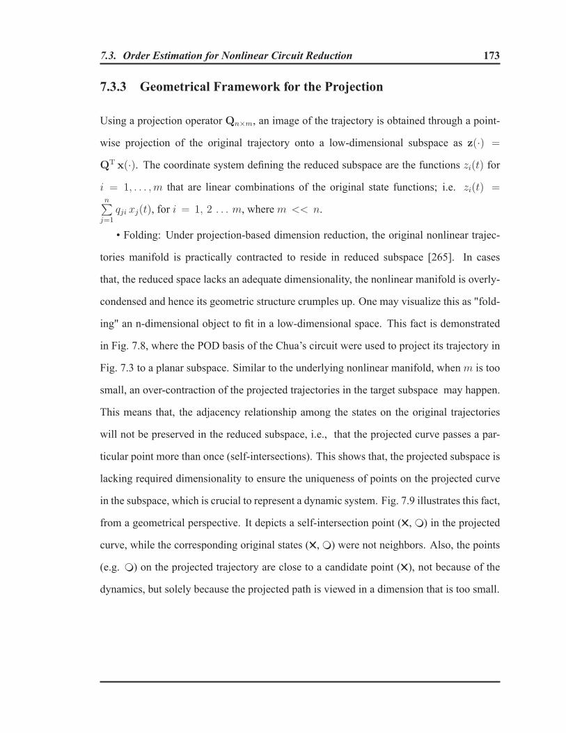
7.3. Order Estimation for Nonlinear Circuit Reduction 173
7.3.3 Geometrical Framework for the Projection
Using a projection operator Qn×m, an image of the trajectory is obtained through a point-
wise projection of the original trajectory onto a low-dimensional subspace as z(·) =
QT x(·). The coordinate system defining the reduced subspace are the functions zi(t) fori = 1, . . . ,m that are linear combinations of the original state functions; i.e. zi(t) =n∑
j=1
qji xj(t), for i = 1, 2 . . . m, wherem << n.
• Folding: Under projection-based dimension reduction, the original nonlinear trajec-
tories manifold is practically contracted to reside in reduced subspace [265]. In cases
that, the reduced space lacks an adequate dimensionality, the nonlinear manifold is overly-
condensed and hence its geometric structure crumples up. One may visualize this as "fold-
ing" an n-dimensional object to fit in a low-dimensional space. This fact is demonstrated
in Fig. 7.8, where the POD basis of the Chua’s circuit were used to project its trajectory in
Fig. 7.3 to a planar subspace. Similar to the underlying nonlinear manifold, whenm is too
small, an over-contraction of the projected trajectories in the target subspace may happen.
This means that, the adjacency relationship among the states on the original trajectories
will not be preserved in the reduced subspace, i.e., that the projected curve passes a par-
ticular point more than once (self-intersections). This shows that, the projected subspace is
lacking required dimensionality to ensure the uniqueness of points on the projected curve
in the subspace, which is crucial to represent a dynamic system. Fig. 7.9 illustrates this fact,
from a geometrical perspective. It depicts a self-intersection point (✕, ❍) in the projected
curve, while the corresponding original states (✕, ❍) were not neighbors. Also, the points
(e.g. ❍) on the projected trajectory are close to a candidate point (✕), not because of the
dynamics, but solely because the projected path is viewed in a dimension that is too small.

7.3. Order Estimation for Nonlinear Circuit Reduction 174
Figure 7.8: Illustration of Chua’s trajectory in Fig.7.7 projected to a two-dimensional sub-space, where its underlying manifold is over-contracted.
Figure 7.9: (left) Illustration of false nearest neighbor (FNN), where the 3-dimensionaltrajectory of the Chua’s circuit in Fig.7.7 is projected; (right) A zoomed-in view of theprojected trajectory.

7.3. Order Estimation for Nonlinear Circuit Reduction 175
7.3.4 Proposed Order Estimation for Nonlinear Reduced Models
To explain the proposed method, first, the concept of the "false nearest neighbor" (FNN)
on a nonlinear manifold needs to be formally defined as the following.
Definition 7.2. The points which are neighbors in the reduced space are defined as “false
neighbors“ when the corresponding states are not neighbors in the original manifold, and
are “true neighbors“ when the corresponding original states are also neighbors in the orig-
inal manifold.
• Unfolding: Based on a geometric intuition, unfolding can be inferred as reversing
the folding process. increasing the dimension of the reduced subspace, e.g. from m = 2
in Fig. 7.8 to m + 1 = 3 in Fig. 7.7 can unfold the geometric structure of trajectory by
distancing the false nearest neighbors such as (✕) and (❍).
Inspired by these observations, the underlying idea in the proposed algorithm is to ge-
ometrically observe the behavior of near neighboring points that are lying on the projected
nonlinear trajectory in an unfolding process. Starting from a low-dimensional subspace,
the order of the reduced space is consecutively increased. In each step, the projected tra-
jectory is expanded into higher dimensions. Consequently, some neighboring points move
far apart and reveal themselves as false nearest neighbors. This is illustrated in Fig. 7.10.
It depicts how neighborhood relations may change by going fromm tom+ 1 (note that in
Fig. 7.10 m = 1). The neighboring point (❍) that is closely located to the reference point
(❑) in Rm is noticeably displaced by the transition to Rm+1 and hence is revealed as false
neighbor.
This process of expansion, ultimately leads to a minimal order mo for which and also
for other higher orders m > mo, only neighbors on the projected trajectory in the reduced
space are true neighbors. In this way, the projected trajectory in anmo-dimensional reduced
space is a one-to-one image of the system trajectory in the original manifold. Thus, the
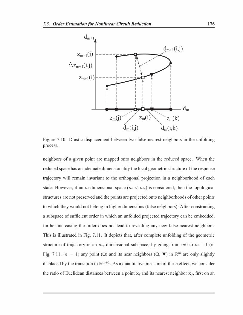
7.3. Order Estimation for Nonlinear Circuit Reduction 176
Figure 7.10: Drastic displacement between two false nearest neighbors in the unfoldingprocess.
neighbors of a given point are mapped onto neighbors in the reduced space. When the
reduced space has an adequate dimensionality the local geometric structure of the response
trajectory will remain invariant to the orthogonal projection in a neighborhood of each
state. However, if an m-dimensional space (m < mo) is considered, then the topological
structures are not preserved and the points are projected onto neighborhoods of other points
to which they would not belong in higher dimensions (false neighbors). After constructing
a subspace of sufficient order in which an unfolded projected trajectory can be embedded,
further increasing the order does not lead to revealing any new false nearest neighbors.
This is illustrated in Fig. 7.11. It depicts that, after complete unfolding of the geometric
structure of trajectory in an mo-dimensional subspace, by going from m0 to m + 1 (in
Fig. 7.11, m = 1) any point (❑) and its near neighbors (❍, ▼) in Rm are only slightly
displaced by the transition to Rm+1. As a quantitative measure of these effect, we consider
the ratio of Euclidean distances between a point xi and its nearest neighbor xj , first on an

7.3. Order Estimation for Nonlinear Circuit Reduction 177
Figure 7.11: Small displacement between every two nearest neighbors by adding a newdimension (m+ 1 or higher), when trajectory was fully unfolded inm dimensional space.
m-dimensional and then on an (m+ 1)-dimensional space, it is [265, 275].
Rij =
[d2m+1(i, j)− d2m(i, j)
d2m(i, j)
] 12
=Δzm+1(i, j)
dm(i, j)(7.7)
Using (7.7), the relative change in distance by adding one more dimension is evaluated as a
mean to decide if the states were not truly close together due to the dynamics but as a result
of projection from a higher state space to smaller space with an inadequate dimension. To
deem xj to be a false nearest neighbor of xi in an m-dimensional subspace the following
should hold.
Rij =Δzm+1(i, j)
dm(i, j)> ρ
FNN(7.8)
where Δzm+1(i, j) � |zm+1(i)− zm+1(j)| and ρFNNis a threshold value.
• Upper bound for the choice of the threshold ρFNN
:
The one parameter that needs to be determined before performing the false nearest
neighbors algorithm is the threshold constant ρFNN
in (7.8). For the FNN algorithm

7.3. Order Estimation for Nonlinear Circuit Reduction 178
to correctly find that there are no false nearest neighbors in the reduced subspace with
adequate order the threshold value should be chosen in a proper range. This subsection
investigates the bounds for this range of selections.
Proposition 7.1. The choice of proper threshold value in the ratio test for the FNN algo-
rithm of the proposed method is bounded to 0 ≤ ρFNN
≤ 1.
Proof. In order to determine an upper bound, let ρmax be a large enough selection such that
all the near neighboring points on the projected trajectory of orderm can hold the following
ration test:
Rij =Δzm+1(i, j)
dm(i, j)≤ ρmax, ∀zi and nearest neighbor zj . (7.9)
From (7.9), we get
Δzm+1(i, j)
dm(i, j)=
|zm+1(i)− zm+1(j)|‖zm(i)− zm(j)‖ =∣∣qT
m+1xi − qTm+1xj
∣∣‖QT
mxi −QTmxj‖ =
|qTm+1 (xi − xj) |
‖QTm (xi − xj) t‖ ≤ ρmax (7.10)
and hence ∣∣qTm+1 (xi − xj)
∣∣ ≤ ρmax‖QTm (xi − xj) ‖ . (7.11)
Considering the consistent matrix norm in (7.11), it is
∣∣qTm+1 (xi − xj)
∣∣ ≤ ρmax‖QTm (xi − xj) ‖ ≤ ρmax‖QT
m‖ ‖ (xi − xj) ‖ . (7.12)

7.3. Order Estimation for Nonlinear Circuit Reduction 179
Due to the property of the 2-norm of orthonormal matrices, for the projection matrixQ
‖QT‖ = ‖Q‖ = 1 . (7.13)
From (7.12) and (7.13);
∣∣qTm+1 (xi − xj)
∣∣ ≤ ρmax‖ (xi − xj) ‖ . (7.14)
Applying Cauchy-Schwarz inequality [276] to the left hand side of (7.12), we get
∣∣qTm+1 (xi − xj)
∣∣ = |〈qm+1, (xi − xj)〉| < ‖qm+1‖‖ (xi − xj) ‖ (7.15)
and considering that the orthogonal projection basis have unity norm ‖qm+1‖ = 1, from
(7.15) ∣∣qTm+1 (xi − xj)
∣∣ < ‖ (xi − xj) ‖ (7.16)
ρmax = 1 can be trivially decided to ensure both (7.16) and (7.15) are hold for any selection
of the (self excluded) neighboring points. Hence it is 0 < ρFNN
< ρmax = 1 that concludes
the proof. �
We established the steps of the proposed nonlinear order estimation in this work based
on the fact that, when the reduced space is of a sufficient dimensionality, such that no false
neighbors are present in the reduced space, a sufficient level of accuracy is ensured for the
nonlinear reduced model. The rigorous justification for this can be formally based on the
followings.
Lemma 7.1. In an orthogonal projection of a nonlinear trajectory the near-neighborhood
of any state on the original manifold are projected to a near neighborhood with smaller
neighborhood radius in the reduced manifold.

7.4. Computational Steps of the Proposed Algorithm 180
This may be referred to as contraction property of projection.
Lemma 7.2. Having all the nearest neighboring points on the projected trajectory as true
neighbors is a necessary and sufficient to ensure the accuracy of reduced nonlinear macro-
model.
The proofs of these lemmas are possible in a similar fashion as the proofs for lemmas 1-
2 in [265] by the authors and the references therein.
Hence, based on the above lemmas the following corollary is concluded.
Corollary 7.1. For nonlinear systems, the order mo is an optimally minimum reduction
order if increasing the order of the reduced subspace to ml, where ml > mo, does not
reveal any false nearest neighboring (FNN) points on the nonlinear reduced trajectory.
The objective of the proposed method is to determine this optimum dimension mo for
the reduced subspace while preserving desired accuracy. The general steps of the proposed
order determination algorithm for nonlinear systems using the FNN are explained in the
Algorithm-1.
7.4 Computational Steps of the Proposed Algorithm
The steps of the proposed algorithm are summarized as follows. For the sake of simplicity
in the notation, hereafter, we drop “t” in the equations (e.g. z(ti) is referred to as z(i)).
Algorithm 2: Proposed Order Estimation Algorithm
Input: X ∈ Rn×N (data matrix from original trajectory)
output: Optimal minimum reduction order (mo)

7.4. Computational Steps of the Proposed Algorithm 181
1 Using the POD algorithm, the projection matrixQ is formed with a small initial
number (m) of orthonormal basis;
2 The time-series data from the projected trajectory is stored in the form
Z = [z(t0), . . . , z(tN)] ∈ Rm×N ;
3 A set of close pointsΠi to each point on the projected trajectory is found based on
the following criteria dm (i, j) < R, for j = 1, · · · , N and j �= i, where R is a
search radius. In general, any choice of R which leads toΠi containing a few close
points is adequate;
4 The number of orthogonal basis is increased fromm tom+ 1 and the new
dimension of the subspace is computed as z(m+1)(·) = qT(m+1)x(·);
5 All the close points z(j) ∈ Πi to z(i) i = 1, . . . , N , that satisfies the following ratio
test are marked as false neighbors Rij =Δzm+1(i, j)
dm(i, j)> ρ
FNN, where ρ
FNNis a
pre-specified threshold value;
6 By repeating the steps (4)-(5), the projected trajectory is expanded into higher
dimensions. Ultimately, at a particular ordermo, the count of false nearest neigh-
bors in step (5) drops to zero, such that, further increasing the order does not lead to
revealing any new false nearest neighbors andmo is selected as the minimum
acceptable order for the reduced model.
The computational steps are summarized in the the flowchart shown in Fig. 7.12. The
flowchart also depicts the interaction between the proposed method and the classical pro-
cess of nonlinear Model reduction, to ensure the parsimony of the model generation cost,
as well as the optimum size for the model.

7.4. Computational Steps of the Proposed Algorithm 182
Start
Read data matrixX =∈ Rn×N
Form projection matrixQ =
[q1, . . . , qms] ∈ R
n×ms
msStarting
order “ms”
Form Z = QT ×X (∈ Rms×n)
Z
Initial Near Neighbors (NN) search
No
Yes
Π
Π �= ∅
Form (m+ 1)th base, qm+1 (∈ Rn×1)
Compute zm+1 = qTm+1 ×X (∈ R
n×1)
FormQ = [Q,qm+1] , Z =
⎡⎣ Z
zm+1
⎤⎦False Nearest Neighbors (FNN)
No
Yes
•
FNN#= 0
OutputQ, m
End
Figure 7.12: Flowchart of the proposed nonlinear order estimation strategy. The grayblocks are the steps of nonlinear MOR interacting with the proposed methods.

7.4. Computational Steps of the Proposed Algorithm 183
From an implementation perspective, the following elaborations are important.
(a) The number of the false nearest neighboring states revealed in the step-5 of Algorithm-1
are traced as a function of the reduced dimension FNN(m). For this purpose, a measure in
a percentage scale is defined as the ratio between the total count of FNN to the total count
of initial near neighbors, i.e.
FNN(m)(%) =numel(Fm)
numel(Π)× 100 (7.17)
where numel(·) returns the number of elements in an array.
(b) Initial Nearest Neigbors (INN) search: Given the transient response data matrix
X = [xi | i ∈ T = {1, . . . , N}] ∈ Rn×N ,
let
Zini = [zi | i ∈ T ] ∈ Rms×N
be the initially projected trajectory, wherems is the starting order for the unfolding process.
For any point on the initially projected trajectory zi ∈ Zini, an array containing its “initial
near neighboring” points is given as
1: for i ← 1 to N do2: for j ← i to N do3: Πi = {j | j ∈ T − {i} and ‖zi − zj‖ < R}5: end for6: end for
where zj ∈ Zini.
The result for the "Initial Nearest Neigbors (NN) search" in the step-3 of Algorithm-2 is
Π =⋃i∈T
Πi.

7.4. Computational Steps of the Proposed Algorithm 184
(c) False Nearest Neigbors (FNN) search: For any point on the projected trajectory of or-
derm (> ms), an array containing its “false near neighbors” is given as
1: for i ← 1 to N do2: if Πi �= ∅ then3: for k ← 1 to numel (Πi) do4: Fm,i =
{j | j = Πi(k) and zi
FNN←→ zj ∈ Zm,}
5: end for6: end if7: end for
Hence, the result from step-5 in Algorithm-2 is Fm =⋃i∈T
Fm,i.
It is sensibly known that, Fm,i ⊆ Πi for any reduced order m, which ensures
FNN(m) ≤ 1.
(d) The following points should also be noted:
d.1) The initial search for close neighbors in the step-3 of Algorithm-2” is performed only
once on the N ×m time series from the projected trajectory, wherem is a small (starting)
order and N is the number of time points (generally, in the range of a few hundreds).
Finding all neighbors in a set of N vectors of sizem can be performed in O (N log(m)) or
O (N) under mild assumptions [260,261].
d.2) The computational complexity of the false nearest neighbors (FNN) search in the
step-5 of Algorithm-2 is O (Nn). In addition, the FNN algorithm is suitable for parallel
implementation, leading to additional reduction in the computational cost [262].
d.3) The proposed method does not require the formulation or simulation of the reduced
macromodel.
d.4) Increasing the number of orthogonal basis from m to m + 1 keeps the initial m basis
unchanged and thus requires the computation of only one new vector.

7.5. Numerical Examples 185
7.5 Numerical Examples
In this section, numerical results are presented to demonstrate the validity and accuracy
of the proposed methodology. To serve this purpose, we consider examples of nonlinear
analog circuits, exhibiting highly nonlinear dynamical behaviors, described by equations
(7.1). Through these examples, it is demonstrated that, by virtue of the estimated order, the
optimally minimum order reduced models ensure efficient and accurate transient behavior
for the resulting reduced model.
In following numerical examples, starting from a reduced space of order two, the count
of false nearest neighbors on the projected trajectory revealed in each step of the unfolding
process (m → m + 1) is monitored. To this end, a measure on a percentage scale (0 to
100) is defined in (7.17).
For the purpose of illustration, Proper Orthogonal Decomposition (POD)
(cf. Algorithm-8) is used as the method of choice in the following numerical exam-
ples. It is to be noted that the proposed method is not limited to any specific nonlinear
projection based algorithm.
7.5.1 Example I
The first example considered is the diode chain network shown in Fig. 7.13-a. The circuit
exhibits significantly nonlinear characteristics and has been considered earlier in [41, 212,
213, 277, 278].The circuit consists of Ns = 302 sections. The values of the resistors and
capacitors are R = 10kΩ and C = 10pF . The diodes are characterized by equation Id =
Is(evdVT − 1), where the saturation current and thermal voltage are given by Is = 10−14A
and VT = 0.0256V , respectively. The state vector is taken as x = [v1, . . . , vN ]T, where
vi is the voltage at node i. A sample of representative input excitations u(t) is shown in

7.5. Numerical Examples 186
Fig. 7.13-b. Applying the proposed method, Fig. 7.14 shows the percentage of the false
(a)
VH = 20V
VL = 5V
tpw = 10nsec.
tf = 1nsec.
(b)
Figure 7.13: (a) Diode chain circuit, (b) Excitation waveform at input.
nearest neighbors on the projected trajectory as defined in (7.17), while the dimension of
the model is changed fromm tom+1. As seen from Fig. 7.14, since reachingm ≥ 13 the
count of false nearest neighbors drops to zero, such that, further increasing the order does
not help the unfolding, and hence does not lead to revealing any new false nearest neighbors
for subsequent orders. Since m = 13 completely unfolds the projected trajectory with no
false neighbors, according to Corollary-7.1, it is selected as the optimum order.
The error between the response (trajectory) obtained from the original system x(org)(·) andits approximation from reduced macromodel x(pod)(·) = Qz(·) is defined as
Error in TrajectoriesΔ=
√√√√√ N∑j=1
n∑i=1
(x(org)i (j)− x
(mor)i (j)
)2
n×N(7.18)

7.5. Numerical Examples 187
Figure 7.14: The percentage of the false nearest neighbors on the projected nonlinear tra-jectory.
where n is the size of the original system and N is the number of time points.
To validate that m = 13 is the optimum order, macromodels of consequent orders are first
generated, followed by variant macromodel-based simulations. The results are compared
against the full simulations. Fig. 7.15 shows the error in the response (7.18) over all the
states obtained from the reduced circuit in (7.18) as function of the order of the reduced
circuit. The FNN graph from Fig. 7.14 is also plotted in the same graph in Fig. 7.15 against
a separate y-axis on the right. The graph clearly depicts thatm = 13 is a minimum order to
ensure the accuracy in the model such that, further increasing the order does not noticeably
improve the accuracy of the model. It is important to notice that, the proposed algorithm
does not require any simulation of the reduced system. Fig. 7.15 is shown only for the
elaboration and validation purposes.
To verify that m = 13 provides an accurate reduced model to properly reproduce the
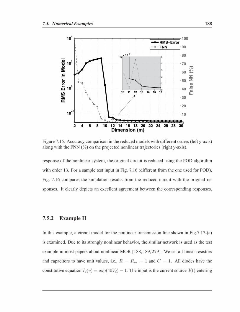
7.5. Numerical Examples 188
Figure 7.15: Accuracy comparison in the reduced models with different orders (left y-axis)along with the FNN (%) on the projected nonlinear trajectories (right y-axis).
response of the nonlinear system, the original circuit is reduced using the POD algorithm
with order 13. For a sample test input in Fig. 7.16 (different from the one used for POD),
Fig. 7.16 compares the simulation results from the reduced circuit with the original re-
sponses. It clearly depicts an excellent agreement between the corresponding responses.
7.5.2 Example II
In this example, a circuit model for the nonlinear transmission line shown in Fig.7.17-(a)
is examined. Due to its strongly nonlinear behavior, the similar network is used as the test
example in most papers about nonlinear MOR [188, 189, 279]. We set all linear resistors
and capacitors to have unit values, i.e., R = Rin = 1 and C = 1. All diodes have the
constitutive equation Id(v) = exp(40Vd)− 1. The input is the current source J(t) entering
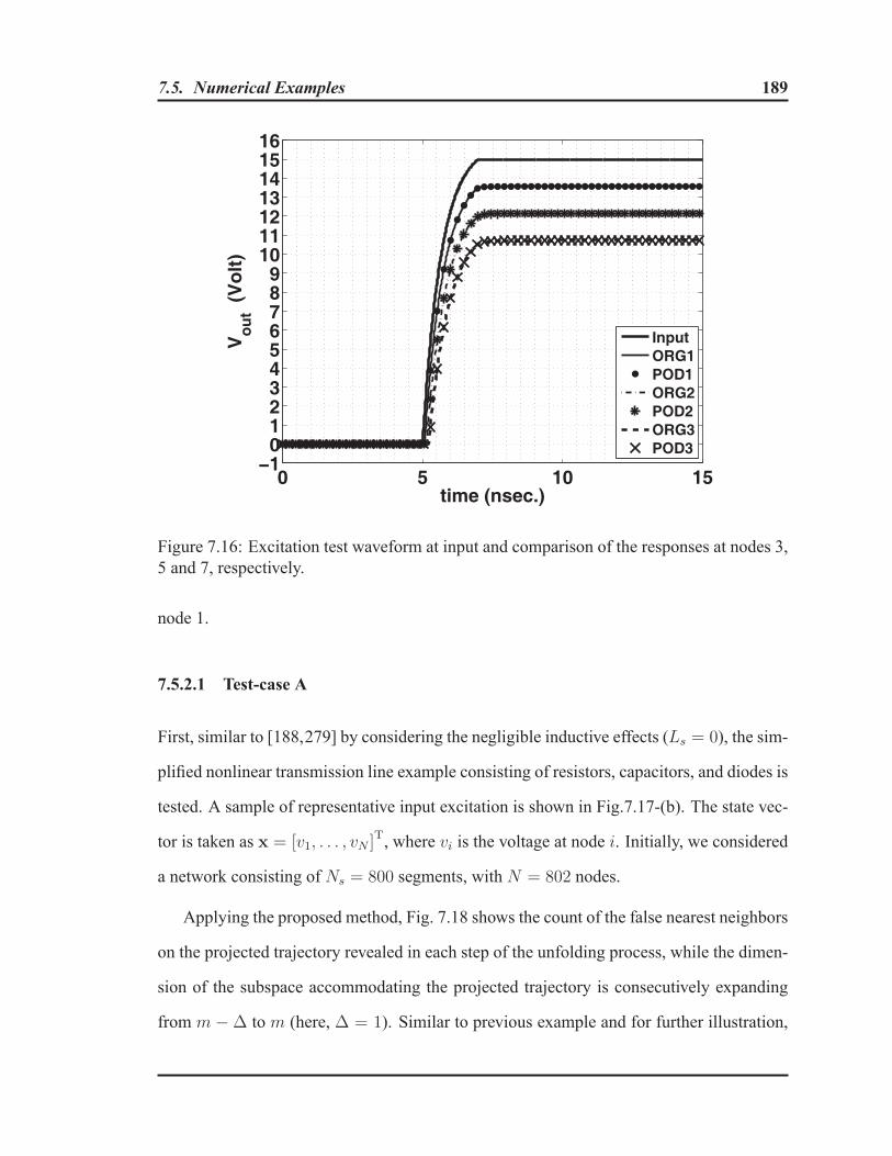
7.5. Numerical Examples 189
0 5 10 15−1
0123456789
10111213141516
time (nsec.)
Vo
ut (
Vo
lt)
InputORG1POD1ORG2POD2ORG3POD3
Figure 7.16: Excitation test waveform at input and comparison of the responses at nodes 3,5 and 7, respectively.
node 1.
7.5.2.1 Test-case A
First, similar to [188,279] by considering the negligible inductive effects (Ls = 0), the sim-
plified nonlinear transmission line example consisting of resistors, capacitors, and diodes is
tested. A sample of representative input excitation is shown in Fig.7.17-(b). The state vec-
tor is taken as x = [v1, . . . , vN ]T, where vi is the voltage at node i. Initially, we considered
a network consisting of Ns = 800 segments, with N = 802 nodes.
Applying the proposed method, Fig. 7.18 shows the count of the false nearest neighbors
on the projected trajectory revealed in each step of the unfolding process, while the dimen-
sion of the subspace accommodating the projected trajectory is consecutively expanding
from m −Δ to m (here, Δ = 1). Similar to previous example and for further illustration,

7.5. Numerical Examples 190
(a)
IH = 10, IL = 1
td = 2, tr = 0.5
tpw = 15, tf = 0.5
(b)
Figure 7.17: (a) Nonlinear transmission line circuit model, (b) Excitation waveform atinput.
in Fig. 7.19, the error in the trajectory (7.18) obtained from the reduced circuits as a func-
tion of the order is shown. The FNN graph from Fig. 7.18 is also illustrated in the same
graph, but against the y-axis on the right. As evidenced by Fig. 7.19, the reduced model at-
tain a commendable level of accuracy only when the projected trajectory is fully unfolded.
This proves m = 15 as the minimum order to ensure the accuracy of the model. To fur-
ther demonstrate that a reduced model of order 15 accurately represents the behavior of the
original system, the reduced (POD) model is tested with the different input in Fig. 7.20-(a)
and the results are shown in Fig. 7.20-(b). The figure clearly depicts an excellent agreement
between the corresponding responses.

7.5. Numerical Examples 191
Figure 7.18: The percentage of the false nearest neighbors on the projected nonlinear tra-jectory.
7.5.2.2 Test-case B
Let us now consider a circuit model of a nonlinear transmission line (cf. Fig. 7.17) com-
prised of Ns = 1500 segments where the inductors connected in series with the resistors
in the segments are L = 10, similar to [189]. I apply the MNA formulation in order to
obtain a dynamical system in form (7.1) of order N = 4502 with voltages at the nodes and
currents in the inductors (branches) of the circuit as circuit variables. A large input signal
is chosen as shown in Fig. 7.21 to ensure that, a rich nonlinear behavior is captured in the
transient response. Fig. 7.22 shows the count of the false nearest neighbors on the projected
trajectory while moving to increasingly larger subspaces. In Fig. 7.23 the error in transient
result of the reduced macromodels with different model sizes is shown along with the FNN
graph, again serving the illustrative purpose here. The two latter figures show m = 29 as

7.5. Numerical Examples 192
Figure 7.19: Accuracy comparison in the reduced models with different orders (left y-axis)along with the FNN (%) on the projected nonlinear trajectories (right y-axis).
the minimum order for the reduced model to guaranty accuracy, signified by consistently
drooping the count of the FNN to zero in the unfolding process. As a second step of ver-
ification, the transient response for the reduced model of order m = 29 is obtained for
the input current J(t) = 2.5(1 − cos5πt), which is significantly different from the POD
"training" input. To further illustrate, Fig. 7.24 shows an excellent agreement between the
responses from the reduced and the original systems.
Figures 7.14 and 7.18 depict that the descending pace of the percentage of false nearest
neighbors is not monotonic. Hence, dropping FNN(%) to zero for just the first time is not
sufficient to decide the order; but it should also remain zero for several subsequent orders.

7.5. Numerical Examples 193
0 5 10 15 20 25 30 35 40 45 500
5
time (sec.)I in
(t) Input
(a)
0 5 10 15 20 25 30 35 40 45 500
0.1
0.2
0.3
0.4
0.5
0.6
0.7
0.8
0.9
1
1.1
time (sec.)
Vo
ut(t
)
ORG1POD1ORG2POD2ORG3POD3ORG4POD4
(b)
Figure 7.20: (a) Excitation test waveform at input, (b) Comparison of the responses atnodes 5, 50, 70, and 200, respectively.
0 5 10 15 20 25 30 35 40 45 5005
1015
time
J(t) Input
Figure 7.21: Excitation waveform at input.

7.5. Numerical Examples 194
Figure 7.22: The percentage of the false nearest neighbors on the projected nonlinear tra-jectory.
��
��
Figure 7.23: Accuracy comparison in the reduced models with different orders (left y-axis)along with the FNN (%) on the projected nonlinear trajectories (right y-axis).

7.5. Numerical Examples 195
0 5 10 15 20 25 30 35 400
0.2
0.4
0.6
0.8
1
time (sec.)
Vo
ut(t
)
ORG1POD1ORG2POD2ORG3POD3
Figure 7.24: Comparison of the responses at output nodes for the segments 30, 60 and 70respectively.

Chapter 8
Conclusions and Future Work
This chapter contains a summary of the work presented in this thesis. In addition, the
possible directions for future work are discussed.
8.1 Conclusions
In this thesis, several new algorithms are presented to address the important issues in the
field of model order reduction for linear and nonlinear systems. The presented algorithms
can be classified into two categories. The first category of algorithms address the issue of
multiport reduction for linear systems. It also deals with the emerging issue of passivity
preservation in the macromodelling of massively coupled multiconductor interconnect net-
works. The second category of algorithms provides novel ways for optimal-order determi-
nation for the reduced linear macromodels as well as the reduced nonlinear models. These
methodologies ensure the accuracy and efficiency of the resulting macromodels when they
are incorporated into an overall circuit simulation and undergo transient analysis.
I. Multiport reduction and clustering:
• The algorithms under this category address various challenging issues which arise in
196

8.1. Conclusions 197
the model order reduction of networks with large number of input/output terminals.
Direct application of the conventional MOR on a multiport network often leads to an
inefficient transient simulation due to the large and dense reduced models. This can
easily undermine the advantage of using MOR. To address this prohibitive issue, a
new, robust, and practical algorithm was presented. The proposed approach is based
on the superposition paradigm for linear systems, and thereby it does not degrade
the level of accuracy expected from the reduction technique of choice. The proposed
algorithm results in reduced models that are sparse and block-diagonal in nature,
leading to faster transient simulations. It is not limited to any specific model order
reduction technique and can work in association with any existing reduction method
of choice. It does not assume any correlation between the responses at ports; and
thereby the algorithm overcomes the accuracy degradation that is normally associated
with the existing terminal reduction techniques. An immediate application for the
proposed algorithms is creating efficient reduced order macromodels for massively
coupled (multiconductor) interconnect networks, such as on-chip data/address buses.
For the latter application, an efficient scheme of clustering was also introduced to
improve the passivity violations that may occur in macromodels.
II. Optimum order determination algorithms for reduced macromodels:
• An algorithm was devised to properly choose the order in the reduction process forlinear networks, which is very important for achieving both efficiency and accuracy.
Guided by geometrical considerations, the new and efficient algorithm was presented
to obtain the optimal order for reduced linear models. It also identifies the redundant
states from the first-level reduction techniques such as PRIMA and thus provides vital
information for a second-level reduction. The application of the proposed method is
not limited to a specific order reduction algorithm and can be used along with any
8.2. Future Research 198
intended projection based methods for linear MOR such as: Krylov-subpace methods
and TBR.
• Estimating an optimal order for the reduced nonlinear model is also of crucial im-portance. To this end, a novel and efficient algorithm has been presented to obtain
the smallest order that ensures the accuracy and efficiency of the reduced nonlinear
model. The proposed method, by deciding a proper order for the projected subspace,
ensures that the reduced model can inherit the dominant dynamical characteristics
of the original nonlinear system. In the proposed method, the False Nearest Neigh-
bors (FNN) approach has been adapted to the case of nonlinear reduction to trace the
deformation of nonlinear manifold in the unfolding process. The proposed method
is incorporated into the projection basis generation algorithm to avoid the computa-
tional cost associated with the extra basis. The proposed nonlinear method works in
conjunction with any intended nonlinear reduced modeling scheme such as: TPWL
with a global reduced subspace, TBR, or POD, etc.
8.2 Future Research
1) Passivity preservation scheme:
The strict diagonal dominance of the transfer function matrix is a sufficient (but not
a necessary) condition for passivity (see, Chapter 5). In practical cases, ensuring
the diagonal dominance for the “Hermitian part” of hybrid transfer function matri-
ces (Z(s) orY(s)) is too restrictive. In Chapter 5, we relaxed this condition to the
block-diagonally strictly dominance . This work can be extended by investigating
less restricted criterion for the enforcement of positive non-negativeness of (Z/Y)
multiport transfer functions.

8.2. Future Research 199
2) Developing an order estimation algorithm in the frequency-domain:
The proposed work can be extended to use the frequency-domain response data to
determine an optimum order for the systems. To achieve this goal a methodology
should be developed to analyze the coherence between neighboring samples through
the state space in the frequency domain.
3) Developing an algorithm that does not need a pre-chosen neighborhood range:
The proposed work can be extended by developing a novel algorithm to reveal the
false nearing neighbors in going from order m to m + 1. The new algorithm will be
independent of any preselected threshold ρFNN . This approach is expected to decide
the optimum reduced order for the resulting model more efficiently.

List of References
[1] N. B. Tufillaro, T. Abbot, and J. Reilly, An Experimental Approach to NonlinearDynamics and Chaos. New York: Perseus Books, 1992.
[2] E. Beltrami, Mathematics for Dynamic Modeling, 2nd ed. San Diego, CA: Aca-demic Press, 1997.
[3] S. H. Strogatz, Nonlinear Dynamics And Chaos: With Applications To Physics, Bi-ology, Chemistry And Engineering. Boulder, CO: Westview Press, 1994.
[4] T. Kailath, Linear Systems. New Jersey: Prentice-Hall, 1980.
[5] C.-T. Chen, Linear System Theory and Design, ser. Oxford Series in Electrical andComputer Engineering, Third, Ed. New York: Oxford University Press, 1998.
[6] L. Perko, Differential Equations and Dynamical Systems, 3rd ed., J. E. Marsden,L. Sirovich, and M. Golubitsky, Eds. New York: Springer, 2006.
[7] F. Verhulst, Nonlinear Differential Equations and Dynamical Systems. New York:Springer, 1990.
[8] E. A. Coddington and N. Levinson, Theory of Ordinary Differential Equations.Malabar, FL: Robert E. Krieger, 1984.
[9] W. Walter, Ordinary Differential Equations. New York: Springer, 1998.
[10] B. D. O. Anderson and S. Vongpanitlerd, Network Analysis and Synthesis. Engle-wood Cliffs, NJ: Prentice Hall, 1973.
[11] D. G. Luenberger, “Dynamic equations in descriptor form,” IEEE Transactions onAutomatic Control, vol. 22, no. 3, pp. 312–321, Jun. 1977.
[12] S. L. Campbell, Singular Systems of Differential Equations, ser. Research Notes inMathematics. London, UK: Pitman Publishing, 1980, vol. 40.
200

201
[13] ——, Singular Systems of Differential Equations II, ser. Research Notes in Mathe-matics. London, UK: Pitman Publishing, 1982, vol. 61.
[14] J. R. Phillips, “Projection-based approaches for model reduction of weakly nonlin-ear, time-varying systems,” IEEE Transactions on Computer-Aided Design of Inte-grated Circuits and Systems, vol. 22, no. 2, pp. 171–187, Feb. 2003.
[15] R. Johansson, System Modeling and Identification. Englewood Cliffs, NJ: Prentice-Hall, 1993.
[16] G.-R. Duan, Analysis and Design of Descriptor Linear Systems, ser. Advances inMechanics and Mathematics. New York: Springer, 2010, vol. 23.
[17] H. K. Khalil, Nonlinear Systems, 3rd ed. Upper Saddle River, NJ: Prentice Hall,2002.
[18] D. G. Luenberger, “Nonlinear descriptor systems,” Journal of Economic dynamicscontrol 1, no. 3, pp. 219–242, Apr. 1979.
[19] N. Tufillaro, “A dynamical systems approach to behavioral modeling,” Hewlett-Packard, Integrated Solutions Laboratory, HP Laboratories Palo Alto, Tech. Rep.HPL-1999-22, Feb. 1999.
[20] J. K. Hedrick and A. Girard, “Control of nonlinear dynamic systems: Theory andapplications,” Berkeley University of California, Berkeley, CA, Course notes (ME-237), Spring 2010.
[21] R. A. Rohrer, Circuit Theory: an introduction to the State Variable Approach. NewYork: McGraw-Hill, 1970.
[22] S. Smale, “On the mathematical foundation of electrical circuit theory,” Journal ofDifferential Geometry, vol. 7, no. 1-2, pp. 193–210, 1972.
[23] E. S. Kuh and R. A. Rohrer, “The state-variable approach to network analysis,” Proc.IEEE, vol. 53, no. 7, pp. 672–686, Jul. 1965.
[24] L. O. Chua, “State variable formulation of nonlinear rlc networks in explicit normalform,” Proc. IEEE, vol. 53, no. 2, pp. 206–207, Feb. 1965.
[25] L. Chua and R. Rohrer, “On the dynamic equations of a class of nonlinear RLCnetworks,” IEEE Transactions on Circuit Theory, vol. 12, no. 4, pp. 475–489, Dec.1965.
202
[26] L. O. Chua, “On the choice of state variables for the potential function in nonlinearnetworks,” Proc. IEEE, vol. 53, no. 12, p. 2110, Dec. 1965.
[27] R. K. Brayton and J. K. Moser, “A theory of nonlinear networks Parts I & II,” Quar-terly of Applied Mathematics, vol. 22, no. 1,2, pp. 1–33, 81–104, Apr./Jul. 1964.
[28] T. Matsumoto, “On several geometric aspects of nonlinear networks,” Journal of theFranklin Institute, vol. 301, no. 1-2, pp. 203–225, Jan.-Feb. 1976.
[29] S. Ichiraku, “Connecting electrical circuits: Transversality and well-posedness,”Yokohama mathematical Journal, vol. 27, no. 5, pp. 111–126, 1979.
[30] T. Matsumoto, L. Chua, H. Kawakami, and S. Ichiraku, “Geometric properties ofdynamic nonlinear networks: Transversality, local-solvability and eventual passiv-ity,” IEEE Transactions on Circuits and Systems, vol. CAS-28, no. 5, pp. 406–428,May 1981.
[31] A. Szatkowski, “On the dynamics of non-linear RLC networks from a geometricpoint of view,” International Journal of Circuit Theory and Applications, vol. 11,no. 2, pp. 117–129, Apr. 1983.
[32] F. H. Branin, “Computer methods of network analysis,” Proc. IEEE, vol. 55, no. 11,pp. 1787–1801, Nov. 1967.
[33] S. R. Sedore, “SCEPTRE: a second generation transient analysis program,” inProc. Computer-Aided Circuit Design Seminar, Cambridge, MA, 1967, pp. 55–61.
[34] C. W. Gear, “The automatic integration of stiff ordinary differential equations,” inProc. the IFIPS Congress, 1968, pp. A81–A85.
[35] I. W. Sandberg and H. Shichman, “Numerical integration of stiff nonlinear differen-tial equation,” Bell System Technical Journal, vol. 47, no. MR38 #1836, pp. 511–527, Apr. 1968.
[36] L. R. Petzold, “Differential/algebraic equations are not ODEs,” SIAM Journal onScientific and Statistical Computing, vol. 3, no. 3, pp. 367–384, Sep. 1982.
[37] J. Vlach and K. Singhal, Computer Methods for Circuit Analysis and Design, 2nd ed.Boston, MA: Kluwer Academic Publishers, 2003.
[38] C.-W. Ho, A. Ruehli, and P. Brennan, “The modified nodal approach to networkanalysis,” IEEE Transactions on Circuits and Systems, vol. 22, no. 6, pp. 504–509,Jun. 1975.

203
[39] L. T. Pillage, R. A. Rohrer, and C. Visweswariah, Electronic Circuit and SystemSimulation Methods. New York: McGraw-Hill, 1994.
[40] M. Striebel and J. Rommes, “Model order reduction of nonlinear systems: status,open issues, and applications,” Technischen Universitat Chemnitz, Chemnitz, Ger-many, Tech. Rep. CSC/08-07, Nov. 2008.
[41] A. Verhoeven, M. Striebel, J. Rommes, E. Maten, and T. Bechtold, “Model orderreduction for nonlinear IC models with POD,” in Progress in Industrial Mathematicsat ECMI 2008, ser. Mathematics in Industry, A. D. Fitt, J. Norbury, H. Ockendon,and E. Wilson, Eds. Berlin, Germany: Springer, 2010, pp. 441–446.
[42] Y. Chen, “Model order reduction for nonlinear systems,” Master thesis, Mas-sachusetts Institute of Technology, Cambridge, MA, Sep. 1999.
[43] A. Verhoeven, E. J. ter Maten, M. Striebel, and R. Mattheij, “Model order reductionfor nonlinear IC models,” in System Modeling and Optimization, ser. IFIP Advancesin Information and Comunication Technology, A. Korytowski, K. Malanowski,W. Mitkowski, and M. Szymkat, Eds. Berlin, Germany: Springer, 2009, vol. 312,pp. 476–491.
[44] W. H. A. Schilders, H. A. van der Vorstand, and J. Rommes, Eds., Model OrderReduction: Theory, Research Aspects and Applications. Berlin, Germany: Springer,2008.
[45] N. Gershenfeld, The nature of mathematical modeling. Cambridge, UK: CambridgeUniversity Press, 1999.
[46] E. A. Bender, An Introduction to Mathematical Modeling. New York: Dover, 2000.
[47] R. Achar and M. Nakhla, “Simulation of high-speed interconnects,” IEEE Proc.,vol. 89, no. 5, pp. 693–728, May 2001.
[48] D. Vasilyev, “Theoretical and practical aspects of linear and nonlinear model or-der reduction techniques,” Ph.D. dissertation, Massachusetts Institute of Technology,Cambridge, MA, Feb. 2008.
[49] D. M. Walker, R. Brown, and N. B. Tufillaro, “A constructing transportable behav-ioral models for nonlinear electronic devices,” Physics Letters A, vol. 255, no. 4-6,pp. 236–242, Feb. 1999.

204
[50] A. L. Walker, “Behavioral modeling and characterization of nonlinear operationin rf and microwave systems,” Ph.D. dissertation, North Carolina State University,Raleigh, NC, 2005.
[51] D. E. R. John Wood, Fundamentals of Nonlinear Behavioral Modeling for RF andMicrowave Design. Boston, MA: Artech House, 2005.
[52] D. E. Root, J. Wood, and N. Tufillaro, “New techniques for non-linear behavioralmodeling of microwave/RF ICs from simulation and nonlinear microwave measure-ments,” in Proc. 40th annual Design Automation Conference, Anaheim, CA, 2003,pp. 85–90.
[53] J. Wood, D. Root, and N. Tufillaro, “A behavioral modeling approach to nonlinearmodel-order reduction for RF/microwave ICs and systems,” IEEE Transactions onMicrowave Theory and Techniques, vol. 52, no. 9, pp. 2274–2284, Sep. 2004.
[54] J. Wood and D. Root, “The behavioral modeling of microwave/rf ics using non-lineartime series analysis,” in Proc. IEEE/MTT-S International Microwave SymposiumDigest, vol. 2, Jun. 2003, pp. 791–794.
[55] S. Sastry, Nonlinear Systems: Analysis, Stability, and Control. New York: Springer,1999.
[56] P. G. Drazin, Nonlinear Systems. Cambridge, MA: Cambridge University Press,1992.
[57] P. J. Antsaklis and A. N. Michel, Linear Systems. Boston, MA: Birkhäuser, 1997.
[58] W. J. Rugh, Linear System Theory, ser. second. Upper Saddle River, NJ: PrenticeHall, 1996.
[59] Y.-L. Jiang and H.-B. Chen, “Time domain model order reduction of general orthog-onal polynomials for linear input-output systems,” IEEE Transactions on AutomaticControl, vol. 57, no. 2, pp. 330–343, Feb. 2012.
[60] J. Cong, L. He, C.-K. Koh, and P. H. Madden, “Performance optimization of VLSIinterconnect layout,” Integration, the VLSI Journal, vol. 21, no. 1&2, pp. 1–94, Nov.1996.
[61] C.-K. Cheng, J. Lillis, S. Lin, and N. Chang, Interconnect analysis and synthesis.Hoboken, NJ: John Wiley, 1999.

205
[62] S. Lee, P. Roblin, and O. Lopez, “Modeling of distributed parasitics in power FETs,”IEEE Transactions on Electron Devices, vol. 49, no. 10, pp. 1799–1806, Oct. 2002.
[63] A. C. Antoulas, Approximation of Large-Scale Dynamical Systems. Philadelphia,PA: SIAM, 2005.
[64] M. Celik, L. Pileggi, and A. Odabasioglu, IC Interconnect Analysis. Norwell, MA:Kluwer, 2002.
[65] S. X.-D. Tan and L. He, Advanced Model Order Reduction Techniques in VLSI De-sign. Cambridge, MA: Cambridge University Press, 2007.
[66] P. Benner, M. Hinz, and E. J. W. ter Maten, Eds., Model Reduction for Circuit Sim-ulation. Berlin, Germany: Springer, 2011.
[67] R. W. Freund, “Reduced-order modeling techniques based on Krylov subspaces andtheir use in circuit simulation,” in Applied and Computational Control, Signals, andCircuits, B. N. Datta, Ed. Boston, MA: Birkhäuser Boston, 1999, vol. 1, ch. 9, pp.435–498.
[68] B. Men, Q. Zhang, X. Li, C. Yang, and Y. Chen, “The stability of linear descriptorsystems,” International Journal of information and systems sciences, vol. 2, no. 3,pp. 362–374, Nov. 2006.
[69] T. Stykel, “Analysis and numerical solution of generalized lyapunov equations,”Ph.D. dissertation, Technischen universität Berlin, Berlin, Germany, Jan. 2002.
[70] D. Debeljkovic, N. Višnjic, and M. R. Pješcic, “The stability of linear continuoussingular systems in the sense of lyapunov: An overview,” Scientific Technical Re-views, vol. LVII, no. 1, pp. 51–64, 2007.
[71] M. R. Wohlers, Lumped and Distributed Passive Networks, H. G. Booker andN. Declaris, Eds. New York: Academic Press, 1969.
[72] S. Boyd, L. E. Ghaoui, E. Feron, and V. Balakrishnan, Linear Matrix Inequalities inSystem and Control Theory. Philadelphia, PA: SIAM, 1994.
[73] P. Triverio, S. Grivet-Talocia, M. Nakhla, F. Canavero, and R. Achar, “Stability,causality, and passivity in electrical interconnect models,” IEEE Transactions onAdvanced Packaging, vol. 30, no. 4, pp. 795–808, Nov. 2007.

206
[74] D. S. Bernstein, Matrix Mathematics: Theory, Facts, and Formulas, 2nd ed. NewJersey: Princeton University Press, 2009.
[75] T. Lyche, “Numerical linear algebra,” University of Oslo, Course Notes Inf-Mat 4350, Aug. 2012.
[76] L. Pillage and R. Rohrer, “Asymptotic waveform evaluation for timing analysis,”IEEE Transactions on Computer-Aided Design of Integrated Circuits and Systems,vol. 9, no. 4, pp. 352–366, Apr. 1990.
[77] V. Raghavan, R. Rohrer, L. Pillage, J. Lee, J. Bracken, and M. Alaybeyi, “AWE-inspired,” in Proc. IEEE Custom Integrated Circuits Conference, May 1993, pp.18.1.1–18.1.8.
[78] E. Chiprout and M. S. Nakhla, Asymptotic Waveform Evaluation. Boston, MA:Kluwer Academic Publishers, 1994.
[79] W. C. Elmore, “The transient analysis of damped linear networks with particularregard to wideband amplifiers,” Journal of Applied Physics, vol. 9, pp. 55–63, Jan.1948.
[80] E. Chiprout and M. S. Nakhla, “Analysis of interconnect networks using complexfrequency hopping,” IEEE Transaction on Computer-Aided Design of IntegratedCircuits and Systems, vol. 14, no. 2, pp. 186–200, Feb. 1995.
[81] P. Feldmann and R. W. Freund, “Efficient linear circuit analysis by Padé approxi-mation via the Lanczos process,” IEEE Transactions on Computer-Aided Design ofIntegrated Circuits and Systems, vol. 14, no. 5, pp. 639–649, May 1995.
[82] R. W. Freund, “Krylov-subspace methods for reduced-order modeling in circuit sim-ulation,” Journal of Computational and Applied Mathematics, vol. 123, no. 1-2, pp.395–421, Nov. 2000.
[83] ——, “SPRIM: structure-preserving reduced-order interconnect macromodeling,” inProc. IEEE/ACM International Conference on Computer-Aided Design, Nov. 2004,pp. 80–87.
[84] L. M. Silveira, M. Kamon, and J. White, “Efficient reduced-order modeling offrequency-dependent coupling inductances associated with 3-D interconnect struc-tures,” IEEE Transactions on Components, Packaging, and Manufacturing Technol-ogy, Part B, vol. 19, no. 2, pp. 283–288, May 1996.
207
[85] A. Odabasioglu, M. Celik, and L. Pileggi, “PRIMA: passive reduced-order intercon-nect macromodeling algorithm,” IEEE Transactions on Computer-Aided Design ofIntegrated Circuits and Systems, vol. 17, no. 8, pp. 645–654, Aug. 1998.
[86] N. L. Schryer, “A tutorial on galerkin’s method, using b-splines, for solving differ-ential equations,” Bell Laboratories, Murray Hill, NJ, Tech. Rep. 52, Sep. 1976.
[87] K. Willcox and J. Peraire, “Balanced model reduction via the proper orthogonaldecomposition,” The American Institute of Aeronautics and Astronautics Journal,vol. 40, no. 11, pp. 2323–2330, Nov. 2002.
[88] C. B. Moore, “Principal component analysis in linear systems: Controllability, Ob-servability, and Model Reduction,” IEEE Transaction on Automatic Control, vol.AC-26, pp. 17–32, Feb. 1981.
[89] C. de Villemagne and R. E. Skelton, “Model reductions using a projection formula-tion,” in Proc. 26th IEEE Conference on Decision and Control, Los Angeles, CA,1987, pp. 461–466.
[90] E. J. Grimme, “Krylov projection methods for model reduction,” Ph.D. dissertation,University of Illinois, Urbana and Champaign, IL, 1997.
[91] Z. Bai, “Krylov subspace techniques for reduced-order modeling of large-scale dy-namical systems,” Applied Numerical Mathematics, vol. 43, no. 1-2, pp. 9–44, 2002.
[92] W. E. Arnoldi, “The principle of minimized iteration in the solution of the matrixeigenvalue problem,” The Quarterly of Applied Mathematics, vol. 9, no. 17, pp. 17–29, 1951.
[93] I. M. Elfadel and D. D. Ling, “A block rational Arnoldi algorithm for multipointpassive model-order reduction of multiport RLC networks,” in Proc. IEEE/ACMinternational conference on Computer-aided design, San Jose, CA, 1997, pp. 66–71.
[94] Y. Saad, Iterative Methods for Sparse Linear Systems, 2nd ed. Philadelphia, PA:Society for Industrial and Applied Mathematics, 2003.
[95] C. Lanczos, “An iteration method for the solution of the eigenvalue problem of lineardifferential and integral operators,” Journal of Research of the National Bureau ofStandards, vol. 45, no. 4, pp. 255–282, Oct. 1950.
208
[96] E. J. Grimme, D. C. Sorensen, and P. V. Dooren, “Model reduction of state spacesystems via an implicitly restarted lanczos method,” Numerical Algorithms, vol. 12,pp. 1–31, 1996.
[97] P. Feldmann and R. W. Freund, “Reduced-order modeling of large linear subcircuitsvia a block lanczos algorithm,” in Proc. 32nd annual IEEE/ACMDesign AutomationConference, San Francisco, CA, Jun. 1995, pp. 474–479.
[98] J. I. Aliaga, D. L. Boley, R. W. Freund, and V. Hernández, “A lanczos-type methodfor multiple starting vectors,” Mathematics of Computation, vol. 69, no. 232, pp.1577–1601, May 2000.
[99] R. W. Freund and P. Feldmann, “Reduced-order modeling of large passive linearcircuits by means of the SyPVL algorithm,” in Proc. IEEE/ACM international con-ference on Computer-aided design, San Jose, CA, Nov. 1996, pp. 280–287.
[100] ——, “The SyMPVL algorithm and its applications to interconnect simulation,” inProc. International Conference on Simulation of Semiconductor Processes and De-vices, Cambridge, MA, Sep. 1997, pp. 113–116.
[101] K. Glover, “All optimal hankel-norm approximations of linear multivariable systemsand their L∞-error bounds,” International Journal of Control, vol. 36, no. 6, pp.1115–1193, Jun. 1984.
[102] D. F. Enns, “Model reduction with balanced realizations: An error bound and afrequency weighted generalization,” in Proc. 23rd IEEE Conference on Decisionand Control, vol. 23, Dec. 1984, pp. 127–132.
[103] A. Laub, M. Heath, C. Paige, and R. Ward, “Computation of system balancingtransformations and other applications of simultaneous diagonalization algorithms,”IEEE Transactions on Automatic Control, vol. 32, no. 2, pp. 115–122, Feb. 1987.
[104] M. G. Safonov and R. Y. Chiang, “A schur method for balanced-truncation modelreduction,” IEEE Transaction Automatic Control, vol. 34, pp. 729–733, Jul. 1989.
[105] C.-A. Lin and T.-Y. Chiu, “Model reduction via frequency weighted balanced real-ization,” in Proc. American Control Conference, May 1990, pp. 2069–2070.
[106] V. Sreeram and B. Anderson, “Frequency weighted balanced reduction technique: ageneralization and an error bound,” in Proc. 34th IEEE Conference on Decision andControl, vol. 4, Dec. 1995, pp. 3576–3581.

209
[107] G. Wang, V. Sreeram, and W. Liu, “A new frequency-weighted balanced trunca-tion method and an error bound,” in Proc. 36th IEEE Conference on Decision andControl, vol. 4, Dec. 1997, pp. 3329–3334.
[108] J.-R. Li and J. White, “Efficient model reduction of interconnect via approximatesystem gramians,” in Proc. EEE/ACM International Conference on Computer-AidedDesign, 1999, pp. 380–383.
[109] J.-R. Li, F. Wang, and J. White, “An efficient lyapunov equation-based approach forgenerating reduced-order models of interconnect,” in Proc. 36th Design AutomationConference, 1999, pp. 1–6.
[110] V. Sreeram, “On the properties of frequency weighted balanced truncation tech-niques,” in Proc. American Control Conference, vol. 3, no. 1753–1754, 2002.
[111] J. Phillips, L. Daniel, and L. M. Silveira, “Guaranteed passive balancing transforma-tions for model order reduction,” in Proc. 39th Annual Design Automation Confer-ence, New Orleans, LA, 2002, pp. 52–57.
[112] J. Phillips, L. Daniel, and L. Silveira, “Guaranteed passive balancing transforma-tions for model order reduction,” IEEE Transactions on Computer-Aided Design ofIntegrated Circuits and Systems, vol. 22, no. 8, pp. 1027–1041, Aug. 2003.
[113] J. Phillips and L. M. Silveira, “Poor man’s TBR" a simple model reduction scheme,”in Proc. European Design and Test Conference, 2004, pp. 938–943.
[114] J. Phillips and L. Silveira, “Poor man’s TBR: a simple model reduction scheme,”IEEE Transactions on Computer-Aided Design of Integrated Circuits and Systems,vol. 24, no. 1, pp. 43–55, Jan. 2005.
[115] N. Wong and V. Balakrishnan, “Fast balanced stochastic truncation via a quadraticextension of the alternating direction implicit iteration,” in Proc. IEEE/ACM Inter-national Conference on Computer-Aided Design, San Jose, CA, 2005, pp. 801–805.
[116] P. Heydari and M. Pedram, “Model-order reduction using variational balanced trun-cation with spectral shaping,” IEEE Transactions on Circuits and Systems I: RegularPapers, vol. 53, no. 4, pp. 879–891, Apr. 2006.
[117] G. H. Golub and C. F. van Van Loan, Matrix Computations, 3rd ed. Baltimore,MD: The Johns Hopkins University Press, 1996.

210
[118] J.-R. Li and J. White, “Low rank solution of lyapunov equations,” SIAM Journal onMatrix Analysis and Applications, vol. 24, no. 1, pp. 260–280, Jan. 2002.
[119] P. Benner, J.-R. Li, and T. Penzl, “Numerical solution of large-scale lyapunov equa-tions, riccati equations, and linear-quadratic optimal control problems,” NumericalLinear Algebra with Applications, vol. 15, no. 9, pp. 755–777, 2008.
[120] A. Lu and E. Wachspress, “Solution of lyapunov equations by alternating directionimplicit iteration,” Computers and Mathematics with Applications, vol. 21, no. 9,pp. 43–58, 1991.
[121] N. S. Ellner and E. L. Wachspress, “Alternating direction implicit iteration for sys-tems with complex spectra,” SIAM Journal on Numerical Analysis, vol. 28, no. 3,pp. 859–870, 1991.
[122] S. V. Brian D. O. Anderson, Network Analysis and Synthesis: a Modern SystemsTheory Approach, 2nd ed. New York: Dover, 2006.
[123] Arnold, W.F., III and A. Laub, “Generalized eigen problem algorithms and softwarefor algebraic riccati equations,” Proc. IEEE, vol. 72, no. 12, pp. 1746–1754, Dec.1984.
[124] G. Wang, V. Sreeram, and W. Liu, “A new frequency-weighted balanced truncationmethod and an error bound,” IEEE Transactions on Automatic Control, vol. 44, no. 9,pp. 1734–1737, Sep. 1999.
[125] M. Loéve, Probability Theory I, 4th ed. New York: Springer, 1977.
[126] H. Hotelling, “Simplified calculation of principal components,” Psychometrika,vol. 1, no. 1, pp. 27–35, 1936.
[127] G. Berkooz, P. Holmes, and J. L. Lumley, “The proper orthogonal decompositionin the analysis of turbulent flows,” Annual Review of Fluid Mechanics, vol. 25, pp.539–575, Jan. 1993.
[128] T. Kim, “Frequency-domain karhunen-loéve method and its application to lineardynamic systems,” American Institute of Aeronautics and Astronautics Journal,vol. 36, no. 11, pp. 2117–2123, 1998.
[129] K. E. Willcox, J. Paduano, J. Peraire, and K. Hall, “Low order aerodynamic mod-els for aeroelastic control of turbomachines,” in Proc. on the American Institute of

211
Aeronautics and Astronautics, Structural Dynamics and Materials (SDM) Confer-ence, vol. 3, no. 2204–2214, St Louis, MO, Apr. 1999.
[130] K. C. Hall, E. H. Dowell, and J. P. Thomas, “Proper orthogonal decomposition tech-nique for transonic unsteady aerodynamic flows,” American Institute of Aeronauticsand Astronautics Journal, vol. 38, no. 10, pp. 1853–1862, 2000.
[131] K. Willcox, “Reduced-order aerodynamic models for aeroelastic control of turbo-machines,” Ph.D. dissertation, Massachusetts Institute of Technology, Cambridge,MA, Feb. 2000.
[132] A. George, J. R. Gilbert, and J. W. H. Liu, Graph Theory and Sparse Matrix Com-putation. New York: Springer, 1993.
[133] A. Antoulas, D. C. Sorensen, and S. Gugercin, “A survey of model reduction meth-ods for large-scale systems,” in Structured Matrices in Mathematics, Computer Sci-ence, and Engineering I, V. Olshevsky, Ed. American Mathematical Society, 2001,ch. III, pp. 193–219.
[134] A. J. Sasane, “Hankel norm approximation for infinite-dimensional systems,” Ph.D.dissertation, University of Groningen, Netherlands, Sep. 2001.
[135] A. Megretski, “Model order reduction,” Massachusetts Institute of Technology,Cambridge, MA, Course Notes (6.242), Fall 2004.
[136] Y. Liu, L. Pileggi, and A. Strojwas, “Model order-reduction of RC(L) interconnectincluding variational analysis,” in Proc. 36th Design Automation Conference, 1999,pp. 201–206.
[137] R. Colgren, “Efficient model reduction for the control of large-scale systems,” in Ef-ficient Modeling and Control of Large-Scale Systems, J. Mohammadpour and K. M.Grigoriadis, Eds. New York: Springer, 2010, ch. 2, pp. 59–72.
[138] C. Coelho, J. Phillips, and L. Silveira, “Robust rational function approximation al-gorithm for model generation,” in Proc. 36th Design Automation Conference, 1999,pp. 207–212.
[139] B. Gustavsen and A. Semlyen, “Rational approximation of frequency domain re-sponses by vector fitting,” IEEE Transactions on Power Delivery, vol. 14, no. 3, pp.1052–1061, Jul. 1999.

212
[140] D. Deschrijver, B. Haegeman, and T. Dhaene, “Orthonormal vector fitting: A robustmacromodeling tool for rational approximation of frequency domain responses,”IEEE Transactions on Advanced Packaging, vol. 30, no. 2, pp. 216–225, May 2007.
[141] S. Grivet-Talocia, “The time-domain vector fitting algorithm for linear macromodel-ing,” AEU-International Journal of Electronics and Communications, vol. 58, no. 4,pp. 293–295, 2004.
[142] S. Grivet-Talocia, F. G. Canavero, I. S. Stievano, and I. A. Maio, “Circuit extractionvia time-domain vector fitting,” in Proc. International Symposium on Electromag-netic Compatibility, vol. 3, Aug. 2004, pp. 1005–1010.
[143] S. Grivet-Talocia, “Package macromodeling via time-domain vector fitting,” IEEEMicrowave and Wireless Components Letters, vol. 13, no. 11, pp. 472–474, Nov.2003.
[144] Y. Mekonnen and J. Schutt-Aine, “Broadband macromodeling of sampled frequencydata using z-domain vector-fitting method,” in Proc. IEEEWorkshop on Signal Prop-agation on Interconnects, Genova, Italy, May 2007, pp. 45–48.
[145] B. Nouri, R. Achar, and M. S. Nakhla, “z-Domain orthonormal basis functionsfor physical system identifications,” IEEE Transactions on Advanced Packaging,vol. 33, no. 1, pp. 293–307, Feb. 2010.
[146] B. Gustavsen and A. Semlyen, “Simulation of transmission line transients usingvector fitting and modal decomposition,” IEEE Transactions on Power Delivery,vol. 13, no. 2, pp. 605–614, Apr. 1998.
[147] B. Gustavsen, “Relaxed vector fitting algorithm for rational approximation of fre-quency domain responses,” in Proc. 10th IEEE Workshop Signal Propagation Inter-connects, Berlin, Germany, May 2006, p. 97âAS100.
[148] ——, “Improving the pole relocating properties of vector fitting,” IEEE Transactionson Power Delivery, vol. 21, no. 3, pp. 1587–1592, Jul. 2006.
[149] D. Deschrijver, M. Mrozowski, T. Dhaene, and D. De Zutter, “Macromodeling ofmultiport systems using a fast implementation of the vector fitting method,” IEEEMicrowave and Wireless Components Letters, vol. 18, no. 6, pp. 383–385, Jun. 2008.
[150] R. Pintelon, P. Guillaume, Y. Rolain, J. Schoukens, and H. Van Hamme, “Parametricidentification of transfer functions in the frequency domain–a survey,” IEEE Trans-actions on Automatic Control, vol. 39, no. 11, pp. 2245–2260, Nov. 1994.

213
[151] S.-B. Nouri, “Advanced macromodeling algorithm for sampled time/frequencydomain measured/tabulated data,” Master’s thesis, Carleton University, Ottawa,Canada, Feb. 2008.
[152] E. C. Levi, “Complex curvefitting,” IEEE Transactions on Automatic Control, vol.AC-4, no. 1, pp. 37–43, Jan. 1959.
[153] C. K. Sanathanan and J. Koerner, “Transfer function synthesis as a ratio of twocomplex polynomials,” IEEE Transactions on Automatic Control, vol. 8, no. 1, pp.56–58, Jan. 1963.
[154] B. Nouri, R. Achar, M. S. Nakhla, and D. Saraswat, “z-Domain orthonormal vec-tor fitting for macromodeling high-speed modules characterized by tabulated data,”in Proc. 12th IEEE Workshop on Signal Propagation on Interconnects, Avignon,France, May 2008, pp. 1–4.
[155] K. C. Sou, A. Megretski, and L. Daniel, “A quasi-convex optimization approach toparameterized model order reduction,” in Proc. 42nd Design Automation Confer-ence, Jun. 2005, pp. 933–938.
[156] ——, “A quasi-convex optimization approach to parameterized model order reduc-tion,” IEEE Transactions on Computer-Aided Design of Integrated Circuits and Sys-tems, vol. 27, no. 3, pp. 456–469, Mar. 2008.
[157] C. Beattie and S. Gugercin, “Interpolatory projection methods for structure-preserving model reduction,” Systems & Control Letters, vol. 58, no. 3, pp. 225–232,2009.
[158] S. Lefteriu and A. C. Antoulas, “A new approach to modeling multiport systemsfrom fequency-domain data,” IEEE Transactions on Computer-Aided Design of In-tegrated Circuits and Systems, vol. 29, no. 1, pp. 14–27, Jan. 2010.
[159] M. Kamon, F. Wang, and J. White, “Generating nearly optimally compact modelsfrom krylov-subspace based reduced-order models,” IEEE Transactions on Circuitsand Systems II: Analog and Digital Signal Processing, vol. 47, no. 4, pp. 239–248,Apr. 2000.
[160] A. Antoulas and D. C. Sorensen, “Approximation of large-scale dynamical system:An overview,” International Journal of Applied Mathematics and Computer Science,vol. 11, no. 5, pp. 1093–1121, 2001.

214
[161] J. A. Martínez, “Model order reduction of nonlinear dynamic systems using multipleprojection bases and optimization state-space sampling,” Ph.D. dissertation, Univer-sity of Pittsburgh, Pittsburgh, PA, Jun. 2009.
[162] S. Gugercin and A. C. Antoulas, “Model reduction of large-scale systems by leastsquares,” Linear Algebra and its Applications, vol. 415, no. 2, pp. 290–321, 2006.
[163] M. F. Selivanov and Y. A. Chernoivan, “A combined approach of the laplacetransform and padé approximation solving viscoelasticity,” International Journal ofSolids and Structures problems, vol. 44, no. 1, pp. 66–76, Mar. 2007.
[164] Y. Kawamura, “IEEE transactions on circuits and systems,” A formulation of non-linear dynamic networks, vol. 25, no. 2, pp. 88–98, Feb. 1978.
[165] T. Matsumoto, “On the dynamics of electrical networks,” Journal of DifferentialEquations, vol. 21, no. 1, pp. 179–196, May 1976.
[166] L. O. Chua, “Dynamic nonlinear networks: State-of-the-art,” IEEE Transactions onCircuits and Systems, vol. CAS-27, no. 11, pp. 1059–1087, Nov. 1980.
[167] F. N. Najm, Circuit Simulation. Hoboken, NJ: Wiley-IEEE Press, 2010.
[168] J.-M. Ginoux,Differential Geometry Applied to Dynamical Systems, L. O. Chua, Ed.Hackensack, NJ: World Scientific, 2009.
[169] M. W. Hirsch, S. Smale, and R. L. Devaney, Differential Equations, Dynamical Sys-tems and an Introduction to Chaos, 2nd ed. San Diego, CA: Academic Press,2004.
[170] B. N. Bond, “Stability-preserving model reduction for linear and nonlinear systemsarising in analog circuit applications,” Ph.D. dissertation, Massachusetts Institute ofTechnology, Cambridge, MA, Feb. 2010.
[171] B. N. Bond and L. Daniel, “Stable reduced models for nonlinear descriptor sys-tems through piecewise-linear approximation and projection,” IEEE Transactionson Computer-Aided Design of Integrated Circuits and Systems, vol. 28, no. 10, pp.1467–1480, Oct. 2009.
[172] ——, “Stabilizing schemes for piecewise-linear reduced order models via projec-tion and weighting functions,” in Proc. IEEE/ACM International Conference onComputer-Aided Design, San Jose, CA, Nov. 2007, pp. 860–867.

215
[173] D. Amsallem and C. Farhat, “Stabilization of projection-based reduced-order mod-els,” International Journal for Numerical Methods in Engineering, vol. 91, no. 4,pp. 358–377, Jul. 2012.
[174] ——, “On the stability of reduced-order linearized computational fluid dynamicsmodels based on POD and galerkin projection: descriptor versus non-descriptorforms,” in Reduced Order Methods for Modeling and Computational Reduction, ser.MS&A Series, A. Quarteroni and G. Rozza, Eds. New York: Springer, 2014, vol. 9,pp. 215–233.
[175] M. Vidyagasar, Nonlinear Systems Analysis, 2nd ed. Englewood Cliffs, NJ:Prentice-Hall, 1993.
[176] J. R. Phillips, “Projection frameworks for model reduction of weakly nonlinear sys-tems,” in Proc. Design Automation Conference, Los Angeles, CA, 2000, pp. 184–189.
[177] A. Mohammad and J. A. De Abreu-Garcia, “A transformation approach for modelorder reduction of nonlinear systems,” in Proc. 16th Annual Conference of IEEEIndustrial Electronics Society, vol. 1, Pacific Grove, CA, Nov. 1990, pp. 380–383.
[178] E. Hung, Y.-J. Yang, and S. Senturia, “Low-order models for fast dynamical simu-lation of MEMS microstructures,” in Proc. International Conference on Solid StateSensors and Actuators, vol. 2, Chicago, IL, Jun. 1997, pp. 1101–1104.
[179] J. Chen and S.-M. Kang, “An algorithm for automatic model-order reduction of non-linear mems devices,” in Proc. IEEE International Symposium on Circuits and Sys-tems, vol. 2, 2000, pp. 445–448.
[180] Y. Chen and J. White, “A quadratic method for nonlinear model order reduction,”in Proc. International Conference on Modeling and Simulation of Microsystems,Semiconductors, Sensors and Actuators,, San Diego, CA, Mar. 2000, pp. 477–480.
[181] Y. Su, J. Wang, X. Zeng, Z. Bai, C. Chiang, and D. Zhou, “SAPOR: second-orderarnoldi method for passive order reduction of RCS circuits,” in Proc. IEEE/ACMInternational Conference on Computer Aided Design, Washington, DC, Nov. 2004,pp. 74–79.
[182] B. Liu, X. Zeng, Y. Su, J. Tao, Z. Bai, C. Chiang, and D. Zhou, “Block SAPOR:

216
block second-order arnoldi method for passive order reduction of multi-input multi-output RCS interconnect circuits,” in Proc. Asia and South Pacific Design Automa-tion Conference, vol. 1, Jan. 2005, pp. 244–249.
[183] Y. Shi, H. Yu, and L. He, “SAMSON: a generalized second-order arnoldi method forreducing multiple source linear network with susceptance,” in Proc. internationalsymposium on Physical design, San Jose, CA, Apr. 2006, pp. 25–32.
[184] L. Feng, “Review of model order reduction methods for numerical simulation ofnonlinear circuits,” Applied Mathematics and Computation, vol. 167, no. 1, pp. 576–591, Aug. 2005.
[185] W. J. Rugh, Nonlinear System Theory, The Volterra/Wiener Approach. Baltimore,MD: Johns Hopkins University Press, 1981.
[186] M. Condon and R. Ivanov, “Krylov subspaces from bilinear representations of non-linear systems,” COMPEL: The International Journal for Computation and Mathe-matics in Electrical and Electronic Engineering, vol. 26, no. 2, pp. 399–406, 2007.
[187] M. J. Rewienski and J. White, “A trajectory piecewise-linear approach to model or-der reduction and fast simulation of nonlinear circuits and micromachined devices,”in Proc. IEEE/ACM International Conference on Conference on Computer-AidedDesign, San Jose, CA, Nov. 2001, pp. 252–257.
[188] ——, “A trajectory piecewise-linear approach to model order reduction and fast sim-ulation of nonlinear circuits and micromachined devices,” IEEE Transactions onComputer-Aided Design of Integrated Circuits and Systems, vol. 22, no. 2, pp. 155–170, Feb. 2003.
[189] D. Vasilyev, M. J. Rewienski, and J. White, “A TBR-based trajectory piecewise-linear algorithm for generating accurate low-order models for nonlinear analog cir-cuits and MEMS,” in Proc. Design Automation Conference, Jun. 2003, pp. 490–495.
[190] ——, “Macromodel generation for BioMEMS components using a stabilized bal-anced truncation plus trajectory piecewise-linear approach,” IEEE Transactions onComputer-Aided Design of Integrated Circuits and Systems, vol. 25, no. 2, pp. 285–293, Feb. 2006.
[191] S. Tiwary and R. Rutenbar, “Scalable trajectory methods for on-demand analogmacromodel extraction,” in Proc. 42nd Design Automation Conference, Jun. 2005,pp. 403–408.

217
[192] ——, “Faster, parametric trajectory-based macromodels via localized linear reduc-tions,” in Proc. IEEE/ACM International Conference on Computer-Aided Design,Nov. 2006, pp. 876–883.
[193] ——, “On-the-fly fidelity assessment for trajectory-based circuit macromodels,” inProc. IEEE Custom Integrated Circuits Conference, San Jose, CA, Sep. 2006, pp.185–188.
[194] T. Bechtold, M. Striebel, K. Mohaghegh, and E. J. W. ter Maten, “Nonlinear modelorder reduction in nanoelectronics: Combination of POD and TPWL,” Proc. AppliedMathematics and Mechanics, vol. 8, pp. 10 057âAS–10 060, May 2008.
[195] S. Dabas, N. Dong, and J. Roychowdhury, “Automated extraction of accurate delay/-timingmacromodels of digital gates and latches using trajectory piecewise methods,”in Proc. Design Automation Conference, Asia and South Pacific, Yokohama, Japan,Jan. 2007, p. 361âAS366.
[196] N. Dong and J. Roychowdhury, “General-purpose nonlinear model-order reduc-tion using piecewise-polynomial representations,” IEEE Transactions on Computer-Aided Design of Integrated Circuits and Systems, vol. 27, no. 2, pp. 249–264, Feb.2008.
[197] Y. Zhang, N. Fong, and N. Wong, “Piecewise-polynomial associated transformmacromodeling algorithm for fast nonlinear circuit simulation,” in Proc. Proc. 18thAsia and South Pacific Design Automation Conference, Yokohama, Japan, Jan. 2013,pp. 515–520.
[198] M. Farooq, L. Xia, F. Hussin, and A. Malik, “Automated model generation of analogcircuits through modified trajectory piecewise linear approach with chebyshev new-ton interpolating polynomials,” in Proc. 4th International Conference on IntelligentSystems Modelling Simulation, Jan. 2013, pp. 605–609.
[199] M. J. Rewienski, “A trajectory piecewise-linear approach to model order reduction ofnonlinear dynamical systems,” Ph.D. dissertation, Massachusetts Institute of Tech-nology MIT, Cambridge, MA, Jun. 2003.
[200] T. Voß, “Model reduction for nonlinear differential algebraic equations,” Mastersthesis, University of Wuppertal, Wuppertal, Germany, 2005.

218
[201] A. Vollebregt, T. Bechtold, A. Verhoeven, and E. ter Maten, “Model order reductionof large scale ODE systems: MOR for ANSYS versus ROM workbench,” in Scien-tific Computing in Electrical Engineering, ser. Mathematics in Industry, G. Ciuprinaand D. Ioan, Eds. Berlin, Heidelberg: Springer, 2007, vol. 11, pp. 175–182.
[202] R. Ionutiu, S. Lefteriu, and A. C. Antoulas, “Comparison of model reduction meth-ods with applications to circuit simulation,” in Scientific Computing in ElectricalEngineering, ser. Mathematics in Industry, G. Ciuprina and D. Ioan, Eds. BerlinHeidelberg: Springer, 2007, vol. 11, pp. 3–24.
[203] T. Voß, A. Verhoeven, T. Bechtold, and J. Maten, “Model order reduction for nonlin-ear differential algebraic equations in circuit simulation,” in Progress in IndustrialMathematics at ECMI 2006, ser. Mathematics in Industry, L. Bonilla, M. Moscoso,G. Platero, and J. Vega, Eds. Berlin, Heidelberg: Springer, 2008, vol. 12, pp.518–523.
[204] K. Mohaghegh, M. Striebel, E. ter Maten, and R. Pulch, “Nonlinear model orderreduction based on trajectory piecewise linear approach: Comparing different linearcores,” in Scientific Computing in Electrical Engineering SCEE 2008, ser. Mathe-matics in Industry, J. Roos and L. R. Costa, Eds. Berlin, Heidelberg: Springer,2010, pp. 563–570.
[205] J. Roychowdhury, “Reduced-order modelling of time-varying systems,” IEEE Trans-actions on Circuits and Systems II: Analog and Digital Signal Processing, vol. 46,no. 10, pp. 1273–1288, Oct. 1999.
[206] J. R. Phillips, “Automated extraction of nonlinear circuit macromodels,” in Proc. theIEEE Custom Integrated Circuits Conference, Orlando, FL, 2000, pp. 451–454.
[207] P. Li and L. Pileggi, “NORM: compact model order reduction of weakly nonlinearsystems,” in Proc. Design Automation Conference, Jun. 2003, pp. 472–477.
[208] K. Pearson, “LIII. on lines and planes of closest fit to systems of points in space,”Philosophical Magazine, Series 6, vol. 2, no. 11, pp. 559–572, 1901.
[209] L. Sirovich, “Turbulence and the dynamics of coherent structures, parts: I-III,”Quar-terly of Applied Mathematics, vol. 45, no. 3, pp. 561–590, Oct. 1987.
[210] P. Astrid, “Reduction of process simulation models: a proper orthogonal decomposi-tion approach,” Ph.D. dissertation, Eindhoven University of Technology, Eindhoven,Netherlands, Nov. 2004.

219
[211] P. Astrid and A. Verhoeven, “Application of least squares mpe technique in the re-duced order modeling of electrical circuits,” in Proc. 17th International SymposiumMathematics Theory of Networks and Systems, Kyoto, Japan, Jul. 2006, pp. 1980–1986.
[212] A. Verhoeven, M. Striebel, and E. Maten, “Model order reduction for nonlinear ICmodels with POD,” in Scientific Computing in Electrical Engineering SCEE 2008,ser. Mathematics in Industry, L. R. Costa and J. Roos, Eds. Berlin/Heidelberg,Germany: Springer, 2008, pp. 571–578.
[213] A. Verhoeven, M. Striebel, J. Rommes, E. Maten, and T. Bechtold, “Proper orthogo-nal decomposition model order reduction of nonlinear IC models,” in Progress inIndustrial Mathematics at ECMI 2008, ser. Mathematics in Industry, A. D. Fitt,J. Norbury, H. Ockendon, and E. Wilson, Eds. Berlin, Germany: Springer, 2010,pp. 441–446.
[214] M. Striebel and J. Rommes, “Model order reduction of nonlinear systems in circuitsimulation: Status and applications,” inModel Reduction for Circuit Simulation, ser.Lecture Notes in Electrical Engineering, P. Benner, M. Hinze, and E. J. W. ter Maten,Eds. Netherlands: Springer, 2011, vol. 74, ch. 17, pp. 289–301.
[215] J. M. Scherpen, “Balancing for nonlinear systems,” Systems and Control Letters,vol. 21, pp. 143–153, 1993.
[216] J. M. Aleida, “Balancing for nonlinear systems,” Ph.D. dissertation, University ofTwente, Enschede, Netherlands, 1994.
[217] J. Hahn and T. Edgar, “Reduction of nonlinear models using balancing of empiricalgramians and galerkin projections,” in Proc. American Control Conference, vol. 4,2000, pp. 2864–2868.
[218] K. Fujimoto and J. M. A. Scherpen, “Nonlinear balanced realization based on singu-lar value analysis of hankel operators,” in Proc. 42nd IEEE Conference on Decisionand Control, vol. 6, Maui, HI, Dec. 2003, pp. 6072–6077.
[219] K. Fujimoto, “On subspace balanced realization and model order reduction for non-linear interconnected systems,” in Proc. IEEE 51st Annual Conference on Decisionand Control, Dec. 2012, pp. 4314–4319.
220
[220] S. Lall, J. E. Marsden, and S. Glavaški, “Empirical model reduction of controllednonlinear systems,” in Proc. IFAC World Congress, Beijing, China, Jul. 1999, pp.473–478.
[221] J. Hahn and T. F. Edgar, “An improved method for nonlinear model reduction us-ing balancing of empirical gramians,” Computers & chemical engineering, vol. 26,no. 10, pp. 1379–1397, Oct. 2002.
[222] M. Condon and R. Ivanov, “Empirical balanced truncation of nonlinear systems,”Journal of Nonlinear Science, vol. 14, no. 5, pp. 405–414, 2004.
[223] N. Nakhla, A. Ruehli, M. Nakhla, and R. Achar, “Simulation of coupled intercon-nects using waveform relaxation and transverse partitioning,” IEEE Transactions onAdvanced Packaging, vol. 29, no. 1, pp. 78–87, Feb. 2006.
[224] N. Nakhla, A. Ruehli, M. Nakhla, R. Achar, and C. Chen, “Waveform relaxationtechniques for simulation of coupled interconnects with frequency-dependent pa-rameters,” IEEE Transactions on Advanced Packaging, vol. 30, no. 2, pp. 257–269,May 2007.
[225] M. Farhan, N. Nakhla, M. Nakhla, R. Achar, and A. Ruehli, “Overlapping partition-ing techniques for simulation of strongly coupled distributed interconnects,” IEEETransactions on Components, Packaging and Manufacturing Technology, vol. 2,no. 7, pp. 1193–1201, Jul. 2012.
[226] A. Dounavis, X. Li, M. Nakhla, and R. Achar, “Passive closed-form transmission-line model for general-purpose circuit simulators,” IEEE Transactions onMicrowaveTheory and Techniques, vol. 47, no. 12, pp. 2450–2459, Dec. 1999.
[227] A. Dounavis, R. Achar, and M. Nakhla, “Efficient passive circuit models for dis-tributed networks with frequency-dependent parameters,” IEEE Transactions on Ad-vanced Packaging, vol. 23, no. 3, pp. 382–392, Aug. 2000.
[228] A. Dounavis, E. Gad, R. Achar, and M. Nakhla, “Passive model reduction of multi-port distributed interconnects,” IEEE Transactions on Microwave Theory and Tech-niques, vol. 48, no. 12, pp. 2325–2334, Dec. 2000.
[229] A. Dounavis, R. Achar, and M. Nakhla, “A general class of passive macromodels forlossy multiconductor transmission lines,” IEEE Transactions on Microwave Theoryand Techniques, vol. 49, no. 10, pp. 1686–1696, Oct. 2001.

221
[230] H. Yu, C. Chu, Y. Shi, D. Smart, L. He, and S.-D. Tan, “Fast analysis of a large-scaleinductive interconnect by block-structure-preserved macromodeling,” IEEE Trans-actions on Very Large Scale Integration (VLSI) Systems, vol. 18, no. 10, pp. 1399–1411, Oct. 2010.
[231] P. Feldmann, “Model order reduction techniques for linear systems with large num-bers of terminals,” in Proc. Design, Automation and Test in Europe Conference andExhibition, vol. 2, Paris, France, Feb. 2004, pp. 944–947.
[232] P. Feldmann and F. Liu, “Sparse and efficient reduced order modeling of linear sub-circuits with large number of terminals,” in Proc. IEEE/ACM International Confer-ence on Computer Aided Design, Nov. 2004, pp. 88–92.
[233] P. Liu, S.-D. Tan, B. Yan, and B. McGaughy, “An extended SVD-based terminal andmodel order reduction algorithm,” in Proc. IEEE International Behavioral Modelingand Simulation Workshop, San Jose, CA, Sep. 2006, pp. 44–49.
[234] P. Liu, S.-D. Tan, H. Li, Z. Qi, J. Kong, B. McGaughy, and L. He, “An efficientmethod for terminal reduction of interconnect circuits considering delay variations,”in Proc. IEEE/ACM International Conference on Computer-Aided Design, Nov.2005, pp. 821–826.
[235] P. Liu, S.-D. Tan, B. McGaughy, and L. Wu, “Compact reduced order modelingfor multiple-port interconnects,” in Proc. 7th International Symposium on QualityElectronic Design, San Jose, CA, Mar. 2006, pp. 413–418.
[236] P. Liu, S.-D. Tan, B. McGaughy, L. Wu, and L. He, “TermMerg: an effi-cient terminal-reduction method for interconnect circuits,” IEEE Transactions onComputer-Aided Design of Integrated Circuits and Systems, vol. 26, no. 8, pp. 1382–1392, Aug. 2007.
[237] B. Nouri, M. S. Nakhla, and R. Achar, “A novel clustering scheme for reduced-ordermacromodeling of massively coupled interconnect structures,” in Proc. IEEE 19thConference on Electrical Performance of Electronic Packaging and Systems, Austin,TX, Oct. 2010, pp. 77–80.
[238] Z. Zhang, X. Hu, C.-K. Cheng, and N. Wong, “A block-diagonal structured modelreduction scheme for power grid networks,” in Proc. Design, Automation Test inEurope Conference and Exhibition, Grenoble, France, Mar. 2011, pp. 1–6.
[239] R. E. Scott, Linear Circuits. New York: Addison-Wesley, 1960.

222
[240] R. W. Newcomb, Linear Multiport Synthesis. New York: McGraw-Hill, 1966.
[241] C.-Y. Zhang, S. Luo, A. Huang, and C. Xu, “The eigenvalue distribution of blockdiagonally dominant matrices and block h-matrices,” Electronic Journal of LinearAlgebra, vol. 20, pp. 621–639, Sep. 2010.
[242] K. Urahama, “Local convergence of waveform relaxation method,” Electronics andCoimnunicatlons in Japan, Part I, vol. 71, no. 2, pp. 52–60, 1988.
[243] S.-H. Xiang and Z.-Y. You, “Weak block diagonally dominant matrices, weak blockH-matrix and their applications,” Linear Algebra and Its Applications, vol. 282, pp.263–274, Oct. 1998.
[244] D. G. Feingold and R. S. Varga, “Block diagonally dominant matrices and general-izations of the Gerschgorin circle theorem,” Pacific Journal of Mathematics, vol. 12,no. 4, pp. 1241–1250, 1962.
[245] D. Saraswat, R. Achar, and M. Nakhla, “Global passivity enforcement algorithm formacromodels of interconnect subnetworks characterized by tabulated data,” IEEETransactions on Very Large Scale Integration (VLSI) Systems, vol. 13, no. 7, pp.819–832, Jul. 2005.
[246] B. Gustavsen, “Passivity enforcement of rational models via modal perturbation,”IEEE Transactions on Power Delivery, vol. 23, no. 2, pp. 768–775, Apr. 2008.
[247] S. Grivet-Talocia and A. Ubolli, “A comparative study of passivity enforcementschemes for linear lumped macromodels,” IEEE Transactions on Advanced Pack-aging, vol. 31, no. 4, pp. 673–683, Nov. 2008.
[248] A. R. Djordjevic, M. B. Bazdar, T. K. Sarkar, and R. F. Harrington, LINPAR forWindows Matrix Parameters for Multiconductor Transmission Lines, Software andUsers’ Manual, Version 2.0. Massachusetts, MA: Artech House Publishers, 1999.
[249] C. R. Paul, Analysis of Multiconductor Transmission Lines, 2nd ed. Hoboken, NJ:John Wiley, 2008.
[250] HSPICE, Synopsis Inc., Mountain View, CA, 2009, ver. C-2009.03.
[251] B. Nouri, M. S. Nakhla, and R. Achar, “A novel algorithm for optimum order esti-mation of reduced order macromodels,” in Proc. 15th IEEE Workshop on Signal andPower Integrity, Naples, Italy, May 2011, pp. 33–36.

223
[252] W. Liebert1, K. Pawelzik, and H. G. Schuster, “Optimal embeddings of chaotic at-tractors from topological considerations,” Europhysics Letter, vol. 14, no. 6, pp.521–526, Mar. 1991.
[253] M. B. Kennel, R. Brown, and H. D. I. Abarbanel, “Determining embedding dimen-sion for phase-space reconstruction using a geometrical construction,” Phys. Rev. A,vol. 45, no. 6, pp. 3403–3411, Mar. 1992.
[254] C. Rhodes and M. Morari, “The false nearest neighbors algorithm: An overview,”Computers and Chemical Engineering, vol. 21, Supplement 1, pp. 1149–1154, 1997.
[255] ——, “False-nearest-neighbors algorithm and noise-corrupted time series,” PhysicalReview E, vol. 55, no. 5, pp. 6162–6170, May 1997.
[256] M. Rathinam and L. Petzold, “A new look at proper orthogonal decomposition,”SIAM Journal on Numerical Analysis, vol. 41, no. 5, pp. 1893–1925, 2003.
[257] T. Aittokallio, M. Gyllenberg, J. Hietarinta, T. Kuusela, and T. Multamäki, “Improv-ing the false nearest neighbors method with graphical analysis,” Physical Review E,vol. 60, no. 1, pp. 416–421, Jul. 1999.
[258] K. Mehlhorn, Multidimensional Searching and Computational Geometry, ser. DataStructures and Algorithms 3, W. Brauer, G. Rozenberg, and A. Salomaa, Eds.Berlin, Germany: Springer, 1984.
[259] S. Arya, D. M. Mount, N. S. Netanyahu, R. Silverman, and A. Y. Wu, “An optimalalgorithm for approximate nearest neighbor searching,” Journal of the ACM, vol. 45,pp. 891–923, Nov. 1998.
[260] T. Schreiber, “Efficient neighbor searching in nonlinear time series analysis,” Inter-national Journal of Bifurcation and Chaos, vol. 5, no. 2, pp. 349–358, Apr. 1995.
[261] H. Kantz and T. Schreiber, Nonlinear Time Series Analysis, 2nd ed. Cambridge,MA: Cambridge University Press, 1997.
[262] I. M. Carrión, E. A. Antúnez, M. M. A. Castillo, and J. J. M. Canals, “A distributedmemory architecture implementation of the False Nearest Neighbors method basedon distribution of dimensions,” The Journal of Supercomputing, vol. 59, no. 3, p.15961618, Mar. 2012.

224
[263] S.-J. Moon and A. Cangellaris, “Order estimation for time-domain vector fitting,” inProc. IEEE 18th Conference on Electrical Performance of Electronic Packaging andSystems, Portland, OR, Oct. 2009, pp. 69–72.
[264] B. Nouri, M. S. Nakhla, and R. Achar, “Efficient reduced-order macromodels ofmassively coupled interconnect structures via clustering,” IEEE Transactions onComponents, Packaging and Manufacturing Technology, vol. 3, no. 5, pp. 826–840,May 2013.
[265] ——, “Optimum order estimation of reduced macromodels based on a geometricapproach for projection-based MOR methods,” IEEE Transactions on Components,Packaging and Manufacturing Technology, vol. 3, no. 7, pp. 1218–1227, Jul. 2013.
[266] C. Desoer and F. Wu, “Trajectories of nonlinear rlc networks: A geometric ap-proach,” IEEE Transactions on Circuit Theory, vol. 19, no. 6, pp. 562–571, Nov.1972.
[267] B. Nouri, M. S. Nakhla, and R. Achar, “A novel algorithm for optimum order esti-mation of nonlinear reduced macromodels,” in Proc. 22nd Electrical Performanceof Electronic Packaging and Systems, San Jose, CA, Oct. 2013, pp. 137–140.
[268] T. Matsumoto, L. Chua, and M. Komuro, “The double scroll,” IEEE Transactionson Circuits and Systems, vol. 32, no. 8, pp. 797–818, Aug. 1985.
[269] R. N. Madan, Ed., Chuas’s Circuit: A Paradigm for Chaos. Singapore: WorldScientific, 1993.
[270] L. Chua, “Nonlinear circuits,” IEEE Transactions on Circuits and Systems, vol. 31,no. 1, pp. 69–87, Jan. 1984.
[271] T. Roska, “On the uniqueness of solutions of nonlinear dynamic networks and sys-tems,” IEEE Transactions on Circuits and Systems, vol. 25, no. 3, pp. 161–169, Mar.1978.
[272] C. Amin, C. Kashyap, N. Menezes, K. Killpack, and E. Chiprout, “A multi-portcurrent source model for multiple-input switching effects in CMOS library cells,”in Proc. 43rd ACM/IEEE Design Automation Conference, San Francisco, CA, 2006,pp. 247–252.
[273] M. Spivak, Calculus On Manifolds: A Modern Approach To Classical Theorems OfAdvanced Calculus, ser. Mathematics Monograph, R. Gunning and H. Rossi, Eds.New York: Addison-Wesley, 1971.

225
[274] L. Conlon, Differentiable Manifolds, ser. Modern Birkhüser Classics. Boston, MA:Birkhäuser, 2008.
[275] C. Rhodes and M. Morari, “Determining the model order of nonlinear input/outputsystems,” AIChE Journal, vol. 44, no. 1, pp. 151–163, 1998.
[276] J. W. Demmel, Applied Numerical Linear Algebra. Philadelphia, PA: Society forIndustrial and Applied Mathematics, 1997.
[277] A. Verhoeven, T. Voss, P. Astrid, E. ter Maten, and T. Bechtold, “Model order reduc-tion for nonlinear problems in circuit simulation,” Proc. Applied Mathematics andMechanics, vol. 7, no. 1, pp. 1 021 603–1 021 604, Dec. 2007.
[278] T. Voss, A. Verhoeven, T. Bechtold, and E. J. ter Maten, “Model order reductionfor nonlinear differential algebraic equations in circuit simulation,” in Progress inIndustrial Mathematics at ECMI 2006, L. L. Bonilla, M. Moscoso, G. Platero, andJ. M. Vega, Eds. Berlin/Heidelberg, Germany: Springer, 2008, pp. 518–523.
[279] B. Bond and L. Daniel, “Parameterized model order reduction of nonlinear dynami-cal systems,” in Proc. IEEE/ACM International Conference on Computer-Aided De-sign, Nov. 2005, pp. 487–494.
[280] E. Kreyszig, Introductory Functional Analysis With Applications. New Jersey: JohnWiley & Sons Inc, 1978.
[281] W. Rudin, Functional Analysis. New York: McGraw-Hill, 1991.
[282] K. Yosida, Functional Analysis, 6th ed. Berlin, Germany: Springer, 1996.
[283] J. B. Conway, A course in functional analysis. Berlin, Germany: Springer, 1985.
[284] A. Megretski and J. Wyatt, “Linear algebra and functional analysis for signals andsystems,” Massachusetts Institute of Technology, Cambridge, MA, Lecture Notes,Sep. 2009.
[285] R. Melrose, “Introduction to functional analysis,” Massachusetts Institute of Tech-nology (MIT-Open Course Ware, Cambridge, MA, Course Notes 18.102, 2009.
[286] M. P. Sanchez. (2013, Apr.) Surjective (version-4). [Online]. Available:http://planetmath.org/Surjective
Appendix A
Properties of Nonlinear Systems in Compare to
Linear
To contrast the behavior of generic linear and nonlinear systems, examples of essentially
nonlinear phenomena [17, 55] are highlighted below:
• Multiple isolated equilibria. A linear system can have only one isolated equilibrium
point; thus, it can have only one steady-state operating point that attracts the state of
the system irrespective of the initial state. A nonlinear system can have more than
one isolated equilibrium point. The state may converge to one of several steady-state
operating points, depending on the initial state of the system.
• Finite escape time. The state of an unstable linear system goes to infinity as time
approaches infinity; a nonlinear system’s state, however, can go to infinity in finite
time.
• Limit cycles. For a linear time-invariant system to oscillate, it must have a pair
of eigenvalues on the imaginary axis, which is a non-robust condition that is almost
impossible to maintain in the presence of perturbations. Even if we do, the amplitude
of oscillation will be dependent on the initial state. In real life, stable oscillation must
226
227
be produced by nonlinear systems. There are nonlinear systems that can go into an
oscillation of fixed amplitude and frequency, irrespective of the initial state. This
type of oscillation is known as a limit cycle.
• Subharmonic, harmonic, or almost-periodic oscillations. A stable linear system
under a periodic input produces an output of the same frequency. A nonlinear system
under periodic excitation can oscillate with frequencies that are submultiples or mul-
tiples of the input frequency. It may even generate an almost-periodic oscillation, an
example is the sum of periodic oscillations with frequencies that are not multiples of
each other.
• Chaos. A nonlinear system can have a more complicated steady-state behavior that
is not equilibrium, periodic oscillation, or almost-periodic oscillation. Such behavior
is usually referred to as chaos. Some of these chaotic motions exhibit randomness,
despite the deterministic nature of the system.
• Multiple modes of behavior. It is not unusual for two or more modes of behavior to
be exhibited by the same nonlinear system. An unforced system may have more than
one limit cycle. A forced system with periodic excitation may exhibit harmonic, sub-
harmonic, or more complicated steady-state behavior, depending upon the amplitude
and frequency of the input. It may even exhibit a discontinuous jump in the mode of
behavior as the amplitude or frequency of the excitation is smoothly changed.

Appendix B
Model Order Reduction Related Concepts
This appendix presents the concepts and techniques that are needed to study the theory of
dynamical systems. It is included to enhance the thoroughness of this thesis in its focus on
the subject of MOR. For more details, interested reader can refer to the given references.
B.1 Tools From Linear Algebra and Functional Analysis
An overview on the mathematical concepts and definitions from “linear algebra” and “func-
tional analysis” [280–285], relevant to the work in this report, is presented.
B.1.1 Review of Vector Space and Normed Space
B.1.1.1 Real and Complex Vector (Linear) Space
Definition B.1 (Vector Space). Consider a nonempty set V of elements of the same type
vi. Elements vi may be vectors in an n-dimensional space, or sequences of numbers, or
functions [280], however it is generally called vectors. The setV = {v1,v2,v3, . . .}. V is
called a vector space or linear space if with respect to two algebraic operations, "addition"
228

B.1. Tools From Linear Algebra and Functional Analysis 229
and "scalar multiplication" the followings properties are satisfied:
(i) V is a closed set under addition: ∀ vi, vj ∈ V, there is (vi + vj ) ∈ V.
Informally it is said, every two vectors (elements) in the set can be added (one to
another) to produce another vector (or element of the same type) in the set.
(ii) V is a closed set under scalar multiplication (scalars are real or complex num-
bers): ∀ vi, ∈ V and each scalar λ ∈ F, there is λvi ∈ V.
Informally it is said, each vector (element) in the set can be scaled with a (real/com-
plex) number and results is an element of the same type, that is in the set.
(iii) Associative: (vi + vj) + vk = vi + (vj + vk), for all vi,vj,vk ∈ V.
(iv) Cumulative: vi + vj = vj + vi, ∀ vi,vj ∈ V.
(v) Distributivity:
(a) λ (vi + vj) = (λvi) + (λvj), ∀ vi,vj ∈ V and λ ∈ F,
(b) (λ + μ)vi = (λvi) + (μvi), ∀ vi ∈ V and λ, μ ∈ F,
(c) λ (μvi) = (λμ) vi, ∀ vi ∈ V and λ, μ ∈ F.
(vi) zero vector: ∃! 0 ∈ V | vi + 0 = vi, ∀ vi ∈ V
(vii) additive inverse: ∀ vi ∈ V ∃ (−vi) ∈ V | vi + (−vi) = 0
(viii) Multiplicative identity: ∃! 0 ∈ V | vi + 0 = vi, ∀ vi ∈ V
• V is called a real vector space, if the scalars come from the field of real numbers
(λ, μ ∈ R).
• V is called a complex vector space, if the scalars come from the field of complex
numbers (λ, μ ∈ C).
A nonempty subset ofV that is a linear space too is called a (linear) subspace ofV.

B.1. Tools From Linear Algebra and Functional Analysis 230
B.1.1.2 Normed and Metric Spaces
Definition B.2 (Normed Space). Let V be a real or complex linear space. A real-valued
function ‖v‖, defined for v ∈ V, is called a norm if it has the properties [9, 284]:
(i) definiteness:
(a) ‖v‖ ≥ 0,
(b) ‖v‖ = 0 ⇔ v = 0,
(ii) homogeneity: ‖λv ‖ = |λ| ‖v‖,(iii) triangle inequality: ‖vi + vj ‖ ≤ ‖vi‖ + ‖vj‖.
The space V is said to be "normed" by ‖ · ‖ [9, 284], and shortly referred to as "normedspace"
Two simple consequences of the triangle inequality are
‖vi + · · · , +vj‖ ≤ ‖vi‖ + . . .+ ‖vj‖ , (B.1)
0 ≤ | ‖vi‖ − ‖vj‖ | ≤ ‖vi − vj‖ . (B.2)
from (B.2), it can explicitly be concluded that,
‖vi‖ − ‖vj‖ ≤ ‖vi − vj‖ . (B.3)
Definition B.3 (Metric Space). A setV together with a real-valued function d : V×V →R as d (vi − vj) = ‖vi − vj‖ is called a metric space and the function d a metric or
distance function, if the following holds:
For all vi, vj , and vk ∈ R,
(i) positivity: d (vi, vj) ≥ 0 . for vi �= vj , and d = (vi,vi)

B.1. Tools From Linear Algebra and Functional Analysis 231
(ii) symmetry: d (vi,vj) = d (vj,vi),
(iii) triangle inequality: d (vi,vj) ≤ d (vi,vk) + d (vk,vj).
It is to be noted that, a "norm" defines a "distance function" (or metric), thus a normed
space is a metric space.
Using this "canonical" distance function and proceeding in a natural manner, we can extend
the definition of familiar mathematical objects from the Euclidean space Rn to any normed
space L. The concepts such as balls, ε-neighborhoods, neighborhoods, interior points,
boundary points, open and closed sets, etc. [9].
B.1.2 Review of the Different Norms
B.1.2.1 Norms for Real Vector Space
An n-dimensional real space Rn which is the set of all n-tuples of real numbers a =
(a1, . . . , an) = (ai) where ai ∈ R can be normed in many ways, e.g., by any one of the
following:
‖a‖2 =√a21 + · · · , + a2n 2-norm , (B.4)
‖a‖1 = |a1| + · · · , + |an| unity-norm , (B.5)
‖a‖∞ = maxi
|ai| maximum-norm. (B.6)
B.1.2.2 Norms for Complex Vector Space
The n-dimensional complex space Cn is normed in the same manner as in previous item,
except in the definition of the the norms as shown in (B.4), it is necessary to use absolute
value as the magnitude of the complex number |a| = |α + jβ| = +√α2 + β2 . For ex-
ample, similar to 2-norm in (B.4), Euclidean-norm for the complex vector space is defined

B.2. Mappings Concepts 232
as
‖a‖e =√|a1|2 + · · · , + |an|2 , Euclidean norm. (B.7)
It is easy to see that, for the case of real vector spaces Euclidean-norm and 2-norm are
equivalent.
B.1.2.3 Norms for Vector Space with Function Elements
It was mentioned that, the elements of a "vector space" may be functions [280]. Hence, the
norm operator for spaces of function should be defined.
LetV = {x(t)} be a set of continuous function defined on the closed interval I (t ∈ I).
The spaceV can be normed in the following ways:
‖x‖I,p =
(∫t∈I
|f(t)|pdt) 1
p
p-norm, (B.8)
‖x‖I,∞ = supt∈I
|x(t)| maximum norm (B.9)
B.2 Mappings Concepts
The concept of “mapping” is fundamentally important in many areas of mathematics, such
as functional analysis and differential geometry [280].
Definition B.4 (Mapping [9,280,281]). LetX,Y be two sets of points in an n-dimensional
space andA ⊆ X and B ⊆ Y be two subsets of them, respectively.
T : X → Y
is a mapping (or transformation) T from A into B, that associates with each x ∈ A a
single y ∈ B as illustrated in Fig. B.1.

B.2. Mappings Concepts 233
If A ⊂ X and B ⊂ Y, T (A) the image of A and T−1 (B) the inverse image or preimage
of B are defined by
T (A) ={y = T(x) | x ∈ A
}, T−1 (B) =
{x| T(x) ∈ B
}.
The set A := DT is called the “domain of definition” of T or, more briefly domain of T.
The set B := RT is also called the range of T. The transformation T(x) may be shorten
as Tx.
A
X Y
B
T
xy =Tx
Figure B.1: Visualization of a mapping
Definition B.5 (Injective or “one-to-one” Mapping [280]). A mapping T is injective, or
one-to-one if every element of the range RT is mapped to by at most one element of the
domain DT.
Notationally, ∀ x1, x2 ∈ DT | x1 �= x2, implies Tx1 �= Tx2. As illustrated in Fig. B.2, it
is said that, different points in DT have different images, so that the inverse image of any
point in RT is a single point in R (T). More mathematically, T is an injective mapping
(iff):
∀ x1, x2 ∈ DT , Tx1 = Tx2 ⇐⇒ x1 = x2 ,
or equivalently, ∀ x1, x2 ∈ DT x1 �= x2 ⇐⇒ Tx1 �= Tx2.

B.2. Mappings Concepts 234
XYT
x1
y1 =Tx1
x2y2 =Tx2
DT
RT
Figure B.2: Visualization of an injective mapping
Definition B.6 (Surjective or “onto” Mapping [280, 286]). A mapping T is called surjec-
tive or a mapping of DT onto Y if RT = Y. This states that, for every y ∈ Y, there is at
least one x ∈ DT such that y = Tx. This is illustrated in Fig B.3.
For example: T: DT −→ RT is always surjective.
XT
DT
RT = Y
Y
Figure B.3: Visualization of an surjective mapping
Definition B.7 (Bijective Mapping [280]). T is bijective if T is both injective (one-to-one)
and surjective (onto).
It is said that there is a one-to-one correspondence between elements in domain and el-
ements in range. If every element of the range is mapped to exactly one element of the

B.2. Mappings Concepts 235
domain as shown in Fig. B.4.
Notationally, ∀ y ∈ Y ∃! x ∈ DT | y = Tx and ∀ x ∈ DT ∃ Tx ∈ Y
XT-1
DT
y=Tx
xRT = Y
Y
Figure B.4: Inverse mapping T−1 : Y −→ D (T) ⊆ X of a bijective mapping T
Definition B.8 (Linear Mappings [9, 281]). An operator T : D → F is called linear if
D is a "linear subspace" of E and T (λx + μy) = λT (x) + μT (y) holds for x, y ∈ D
and λ, μ ∈ R or C.
Definition B.9 (Continuous Operator [9]). An operator T : D → F is said to be con-
tinuous at a point x0 ∈ D if xn ∈ D, xn −→ x0 implies that Txn −→ Tx0.
Remark B.1. For every ε > 0, there exists δ > 0 such that from x ∈ D, ‖x − x0‖ < δ, it
follows that ‖Tx− Tx0‖ < ε [9].
Remark B.2 (Lipschitz Condition for Operators [9]). An operator T satisfies a Lipschitz
condition inD (with Lipschitz constant q) if
‖Tx − Ty‖ ≤ q ‖x − y‖ , for x, y ∈ D (B.10)
It is easy to check that such an operator is continuous inD.
B.2. Mappings Concepts 236
Example B.1. Consider Tf =1∫0
f (x) dx, where f(x) is a continuous function in D =
C ([0, 1]), and F = R. This operator T : D → R is continuous.
Solution:
for f1 = f (x1) and f2 = f (x2) ∈ D, we have
‖Tf1 − Tf2‖ =
∥∥∥∥∥∥1∫
0
f1 dx −1∫
0
f2 dx
∥∥∥∥∥∥︸ ︷︷ ︸norm on F
≤1∫
0
norm on D︷ ︸︸ ︷‖f1 − f2‖ dx = ‖f1 − f2‖,
Lipschitz constant can be picked (e.g.) as q = 1, hence, satisfying Lipschitz condition T
is continuous inD. ■
Definition B.10 (Contractive Mapping). Given a mapping T : D −→ F as
T(x) = x, (B.11)
whereF is a suitably chosen Banach space andD ⊂ F. This mapping is called contractive
(or a contraction) if it satisfies Lipschitz condition (cf. Remark-B.2) on D with Lipschitz
constant q < 1 , i.e.:
∀ x, y ∈ D ∃ q < 1 : ‖Tx − Ty‖ ≤ q ‖x − y‖ . (B.12)
From (B.12) one may say that the distance between the image points Tx and Ty, under
the mapping is smaller by a factor q than the distance between the two original points x,y
and hence T “contracts” distances between points.
Example B.2. Consider mapping T: [0, 1] → [0, 1], with the mapping operator Tx =
1 − x2.
B.2. Mappings Concepts 237
Solution:
For any x, y ∈ [0, 1], we have |Tx− Ty| = ∣∣x2− y
2
∣∣ = 12|x− y| , so, q = 1
2, having
the Lipschitz constant q = 12< 1 then it is Lipschitz and contractive. ■
The solution of (B.11) is called fixed point of mapping T. It is a point which remains
“fixed” under the map T. Fixed points can be found using an iteration procedure called
the method of successive approximation. To find x satisfying x = T(x), it starts from an
element x0 ∈ D and successively forms
x1 = T(x0) , x2 = T(x1) , . . . ,xn+1 = T(xn) , . . . . (B.13)
The convergence of the sequence in (B.13) (to the fixed point x), is intimately connected
to the contracting of mapping.
Example B.3. Does the mapping T(x) = 1 − x2on [0, 1] (in example-B.2) converge?
Solution:
Let x0 = 14→ x1 = 7
8→ x2 = 9
16→ . . ., i.e. lim
x→∞xn = 2
3= X (fixed point).
■
Theorem B.1 (Fixed Point Theorem). LetD be a nonempty, closed set in a Banach space
F. Let the operator T : D −→ F map D into itself, T(D) ⊂ D. Given x0 ∈ D the
sequence xn = Txn+1 converges to a unique value x inD for the fixed point of mapping
such that Tx = x
Proof. For the proof [9, pp.59-60] can be referred to. �

Appendix C
Proof of Theorem-5.1 in Section 5.4
The subsystems in the proposed methodology (5.12) share the sameG andCmatrices with
the original system, i.e. Gi = G and Ci = C, (for i = 1, . . . , K). However, for the sake
of the clarity when following the proof; hereafter, matrices for every i-th subsystem will be
signified with its index i.
For the system in (5.12), let s0 ∈ C be a properly selected expansion point such that
the matrix pencil (Gi + s0Ci) is nonsingular. The corresponding input-to-state transfer
function is obtained by applying Laplace transformation on (5.12a) as
Hi(s) = (Gi + sCi)−1
Bi . (C.1)
From (C.1) and following the similar steps shown in (5.4)-(5.6), the following matrices are
defined
Ai � (Gi + s0Ci)−1
Ci (C.2)
and
Ri � (Gi + s0Ci)−1
Bi . (C.3)
Consider the complex-valued matrix function in (C.1) be a smooth (continuously derivable)
238

239
with invertible (Gi + s0Ci). Its Taylor series approximationHi(s), in the proximity of s0,
can be represented by the expansion
Hi(s) =∞∑j=0
(−1)jMi,j(s0)(s− s0)j (C.4)
where the j-th moment of the function at s0 is
Mi,j(s0) = Aji Ri , (for all j). (C.5)
Similarly, expanding the approximant transfer function (5.26) about s0 gives
Hi(s) =∞∑j=0
(−1)jMi,j(s0)(s− s0)j , (C.6)
where
Mi,j (s0) = QiAji Ri , (for all j) (C.7)
and matrices are given by
Ai �
(Gi + s0Ci
)−1
Ci (C.8)
and
Ri �
(Gi + s0Ci
)−1
Bi . (C.9)
Next, we show that the firstMi = �qi/mi� coefficient matrices (block moments) in theexpansions (C.4) and (C.6) are identical. To serve this purpose, we first define the following
proposition C.1 and lemma C.1, which are used later in the proof of theorem 5.1.
Proposition C.1. Let Qi be a N × qi full column-rank projection matrix, whose columns

240
span the qi dimensional Krylov subspace, as
colspan {Qi} = KMi(Ai,Ri)
= span{Ri, AiRi, . . . , A
Mi−1i Ri
}, (C.10)
whereRi hasmi columns. There exists a N ×mi matrix Ei,j , such that
AjiRi = QiEi,j , 0 ≤ j < Mi . (C.11)
Proof. From the definition of Krylov subspace (C.10) it is deduced that, associated with
every (j-th) moment, there exists a projection of it in the Krylov subspace. Let a N ×mi
matrix Ei,j be the projection of the block momentMi,j into Krylov subspace, induced by
Ai andRi. We thus have
Mi,j = QiEi,j . (C.12)
Substituting (C.5) in (C.12) proves the relationship in (C.11). �
Lemma C.1. Given the projection matrix Qi as specified in proposition C.1, a N × N
matrix as
Fi � Qi (Q∗iGiQi + s0Q
∗iCiQi)
−1Q∗
iCi (C.13)
satisfies the relation
FjiRi = A
jiRi, 0 ≤ j < Mi . (C.14)
Proof. The proof is possible by induction on j. First, it is trivial to prove (C.14) for j = 0.
Next, assume that (C.14) is true for any j − 1 when 0 < j < Mi, that is
Fj−1i Ri = A
j−1i Ri. (C.15)
241
Multiplying both sides of (C.15) byAi in (C.2) yields
(Gi + s0Ci)−1
Ci × Fj−1i Ri = A
jiRi . (C.16)
Substituting (C.11) from proposition C.1 in (C.15), we have
(Gi + s0Ci)−1
Ci × Fj−1i Ri = QiEi,j . (C.17)
Multiplying both sides of (C.17) with a N × N matrix
Qi (Q∗iGiQi + s0Q
∗iCiQi)
−1Q∗
i (Gi + s0Ci) , where superscript ∗ denotes the con-
jugate (Hermitian) transpose, we obtain
Qi (Q∗iGiQi + s0Q
∗iCiQi)
−1Q∗
i (Gi + s0Ci)× (Gi + s0Ci)−1
Ci × Fj−1i Ri =
Qi (Q∗iGiQi + s0Q
∗iCiQi)
−1Q∗
i (Gi + s0Ci)QiEi,j , (C.18)
then,
Qi (Q∗iGiQi + s0Q
∗iCiQi)
−1Q∗
iCi × Fj−1i Ri = QiEi,j . (C.19)
Using (C.11) and (C.13), (C.19) leads to FjiRi = A
jiRi which is the desired relation in
(C.14). �
Following the proposition C.1 and lemma C.1 established above, theorem 5.1 is proved.
Proof of theorem 5.1. In this proof we establish that
Mi,j (s0) = Mi,j (s0) , 0 ≤ j < Mi . (C.20)
I) For j = 0 : To show that the first two block moments are equal, for j = 0, from

242
proposition C.1, we recall that
Ri = QiEi,0 . (C.21)
Multiplying both sides of (C.21) by the matrix Qi (Q∗iGiQi
+s0Q∗iCiQi)
−1Q∗
i (Gi + s0Ci) , used in the proof of lemma C.1, we have
Qi (Q∗iGiQi + s0Q
∗iCiQi)
−1Q∗
i (Gi + s0Ci)×Ri
= Qi (Q∗iGiQi + s0Q
∗iCiQi)
−1Q∗
i (Gi + s0Ci)QiEi,0 . (C.22)
SubstitutingRi from (C.3),
Qi (Q∗iGiQi + s0Q
∗iCiQi)
−1Q∗
i (Gi + s0Ci)× (Gi + s0Ci)−1
Bi =
Qi (Q∗iGiQi + s0Q
∗iCiQi)
−1Q∗
i (Gi + s0Ci)QiEi,0 , (C.23)
it will be
Qi (Q∗iGiQi + s0Q
∗iCiQi)
−1Q∗
iBi = QiEi,0 . (C.24)
Next, substituting (C.21) in (C.24), we get
Qi (Q∗iGiQi + s0Q
∗iCiQi)
−1Q∗
iBi = Ri . (C.25)
Also, combining (5.14), (C.9) and (C.25), we get
QiRi = Ri . (C.26)
According to the definition of the moments for the original and reduced system in (C.5)
and (C.7), respectively, (C.26) can be rewritten as Mi,0 = Mi,0 , that establishes the
matching of the first block moments.

243
II) For 0 < j < Mi : From (C.7), (C.8) and (C.9), we have
Mi,j = Qi ×((
Gi + s0Ci
)−1
Ci
)j
×(Gi + s0Ci
)−1
Bi. (C.27)
Using the definitions of the reduced matrices in (5.14), (C.27) can be rewritten as
Mi,j = Qi
((Q∗
iGiQi + s0Q∗iCiQi)
−1Q∗
iCiQi
)j ×(Q∗
iGiQi + s0Q∗iCiQi)
−1Q∗
iBi , (C.28)
which equivalently is
Mi,j =(Qi (Q
∗iGiQi + s0Q
∗iCiQi)
−1Q∗
iCi
)j ×Qi (Q
∗iGiQi + s0Q
∗iCiQi)
−1Q∗
iBi . (C.29)
Next, substituting (C.13) and (C.25) in (C.29), we get
Mi,j = FjiRi . (C.30)
The result from substituting (C.14) from lemma C.1 in (C.30) and using (C.5) establishes
(C.20). �

Appendix D
Proof of Theorem-5.2 in Section 5.4
Based on the superposition paradigm, the output(s) of the original system can be con-
structed by superposing the responses from the subsystems
I(s) =K∑i=1
Ii(s) . (D.1)
From (D.1) and definition of transfer function, we get
H(s)U(s) = H1(s)U1(s) +H2(s)U2(s) + · · ·+HK(s)UK(s), (D.2)
which equivalently can be written as
H(s)U(s) = [H1(s), H2(s), · · · , HK(s)]
⎡⎢⎢⎢⎢⎢⎢⎢⎢⎢⎢⎢⎢⎢⎢⎣
U1(s)
U2(s)
...
UK(s)
⎤⎥⎥⎥⎥⎥⎥⎥⎥⎥⎥⎥⎥⎥⎥⎦
244

245
= [H1(s), H2(s), · · · , HK(s)]U(s) . (D.3)
Applying Laplace transformation to (5.12), the (input-to-output) transfer function matrix
for any i-th submodel is
Hi(s) = L (Gi + sCi)−1
Bi . (D.4)
Considering the relation in (C.1), from (D.4) we have
Hi(s) = LHi(s) . (D.5)
From (D.3) and (D.5), it is
H(s) = [H1(s), H2(s), · · · , HK(s)]
= L [H1(s), H2(s), · · · , HK(s)] . (D.6)
By expanding the matrix transfer function H(s) in (D.6) in the form of Taylor series in
proximity of the complex frequency s0 and considering (5.7), we get
H(s) = L∑j
(−1)jMj(s0) (s− s0)j =
∑j
(−1)j L[M1,j(s0), · · · , MK,j(s0)
](s− s0)
j (D.7)
By equating the moments in the corresponding terms of the Taylor series in the both sides of
(D.7), the original moments in (5.8) are now obtained based on the corresponding moments
of the submodels, as
Mj(s0) = L[M1,j(s0), · · · , MK,j(s0)
](D.8)

246
Substituting (C.20) in (D.8), we get
Mj(s0) = L[M1,j(s0), · · · , MK,j(s0)
], 0 ≤ j < Mi . (D.9)
Next, the (input-to-output) transfer function for the reduced submodels in (5.13) is obtained
as
Hi(s) = Li
(Gi + sCi
)−1
Bi (D.10)
and considering the definition of Li in (5.14), we have
Hi(s) = LQi
(Gi + sCi
)−1
Bi . (D.11)
By comparing (5.26) and (D.11), it is
Hi(s) = LHi(s) . (D.12)
Then, starting from
I(s) =K∑i=1
Ii(s) . (D.13)
and following the similar steps in (D.2)-(D.6), we get
H(s) = L[H1(s), · · · , HK(s)
](D.14)
The Taylor expansion in proximity of s0 for H(s) in (5.26) and (D.14) leads to
H(s) =∑j
(−1)jLMj(s0) (s− s0)j =
∑j
(−1)jL[M1,j(s0), · · · , MK,j(s0)
](s− s0)
j (D.15)

247
As explained before, by equating the corresponding moment matrices in the both sides of
(D.15), we have
Mj(s0) = L[M1,j(s0), · · · , MK,j(s0)
](D.16)
Comparing (D.9) and (D.16) indicates that, the corresponding entries in the moments ma-
tricesMj(s0) in (D.9) and Mj(s0) in (D.16) are equal for 0 ≤ j < M, which explicitly
proves that these two moment matrices are identical up to a certain orderM.
Mj(s0) = Mj(s0), for 0 ≤ j < M (D.17)
The order of matching M is decided by the lowest count of the moments Mi, matched
between the subsystems and their associated reduced models asM = mini=1,...,K
(Mi). ■