advanced modulation techniques for scaling up multiuser...
TRANSCRIPT

Advanced Modulation Techniques For Scaling UpMultiuser MIMO Communications
J.C. De Luna Ducoing
Submitted for the Degree ofDoctor of Philosophy
from theUniversity of Surrey
Institute for Communication SystemsFaculty of Engineering and Physical Sciences
University of SurreySurrey, U.K.
January 2018
c© J.C. De Luna Ducoing 2018


Declaration of Originality
This thesis and the work to which it refers are the results of my own efforts. Any ideas,data, images or text resulting from the work of others (whether published or unpub-lished) are fully identified as such within the work and attributed to their originatorin the text, bibliography or in footnotes. This thesis has not been submitted in wholeor in part for any other academic degree or professional qualification. I agree that theUniversity has the right to submit my work to the plagiarism detection service Turnit-inUK for originality checks. Whether or not drafts have been so-assessed, the Universityreserves the right to require an electronic version of the final document (as submitted)for assessment as above.
Juan Carlos De Luna Ducoing
September 29, 2017

Abstract
Multiuser multiple-input multiple-output (MU-MIMO) has the potential to substan-tially increase the uplink network efficiency by multiplexing the user terminals’ (UTs)transmissions in the spatial domain. However, demultiplexing the transmissions at thenetwork side, known as MU-MIMO detection, can become a considerable signal pro-cessing challenge, especially in cases with a high spatial user load. During the last twodecades, the MIMO detection problem has been extensively studied, and many receiverdesigns have been proposed that offer very good tradeoffs in complexity vs. performance.Nevertheless, MU-MIMO detection still presents challenges in signal processing scala-bility in the number of antennas and modulation order. We revisit this problem butthrough an alternative method of joint transmitter and receiver design. Two approachesthat exhibit near-optimal reliability and low complexity are presented:
First, a technique that uses real-valued modulation in fully- and over-loaded cases inlarge MU-MIMO systems, where there are equal or more UTs than service antennas.It is seen that the use of real constellations with a widely linear equaliser benefits froman increased spatial diversity gain over complex constellations with a linear equaliser.Moreover, a likelihood ascent search (LAS) algorithm post-processing stage is applied tofurther improve the error performance. Computer simulations show remarkable resultsfor large MU-MIMO sizes in uncoded or coded cases.
Second, recognising that real-valued modulation offers poor modulation efficiency, areal-complex hybrid modulation (RCHM) scheme is proposed, where a mix of real- andcomplex-valued symbols are interleaved in the spatial and temporal domains. It is seenthat RCHM combines the merits of real and complex modulations and enables the ad-justment of the diversity-multiplexing tradeoff. Through the system outage probabilityanalysis, the optimal ratio of the number real-to-complex symbols, as well as their op-timal power allocation, is found for the RCHM pattern. Furthermore, reliability isimproved with a small expense in complexity through the use of a successive interfer-ence cancellation (SIC) stage. Results are validated through the mathematical analysisof the average bit error rate and through computer simulations considering single andmultiple base station scenarios, which show SNR gains over conventional approaches inexcess of 5 dB at 1% BLER.
The results suggest that an expense in complexity is not the only way to improve errorperformance, but near-optimal reliability is also possible using simple techniques througha reduction in the multiplexing gain. Therefore, rather than a two-way complexityvs. performance tradeoff in MU-MIMO detection, a three-way tradeoff may be moreappropriate, and is roughly expressed in the following statement:
“Low complexity, high reliability, high multiplexing gain: choose two.”
Key words: Multiuser multiple-input multiple-output (MU-MIMO), detection, widelylinear (WL) receiver, real-complex hybrid modulation (RCHM), successive interferencecancellation (SIC), likelihood ascent search (LAS).

Acknowledgements
First and foremost, I would like to thank my principal supervisor, Dr. Yi Ma, for hisguidance throughout my PhD program journey. I truly thank him for his near-absoluteavailability, contagious enthusiasm for research, utter patience, profound dedication tohis students and for setting an example of how to be a successful researcher.
I am also grateful to my co-supervisors: Dr. Na Yi for her support and for sharing herknowledge and experience; and Prof. Rahim Tafazolli for his leadership and for allowingme the privilege of having been a part of the prestigious Institute for CommunicationSystems (ICS). To my three supervisors, I am forever indebted.
I also thank my colleagues and teammates at the ICS for their support, helpful discus-sions, and for their camaraderie that comes from being in the same boat as me.
On a personal note, I would like to thank my friends and family, including, but notlimited to: my mother and father for their boundless love and unfailing support; my sonCarlos and my daughter Mariana, who are my pride and joy, I take this opportunity toremind them to always follow their dreams; and last but not least, my wife Sonia, forher endless love and encouragement, any accomplishment is as much hers as it is mine.

Contents
List of Figures viii
List of Tables ix
List of Abbreviations x
1 Introduction 1
1.1 Background . . . . . . . . . . . . . . . . . . . . . . . . . . . . . . . . . . . 1
1.2 Motivation and Objective . . . . . . . . . . . . . . . . . . . . . . . . . . . 2
1.3 Contributions . . . . . . . . . . . . . . . . . . . . . . . . . . . . . . . . . . 5
1.4 Thesis Organisation . . . . . . . . . . . . . . . . . . . . . . . . . . . . . . 8
1.5 Research Outputs . . . . . . . . . . . . . . . . . . . . . . . . . . . . . . . . 8
2 State-of-the-Art 10
2.1 Uplink MU-MIMO System Model . . . . . . . . . . . . . . . . . . . . . . . 11
2.2 MIMO Capacity and Channel Matrix Condition . . . . . . . . . . . . . . . 12
2.2.1 The Marcenko-Pastur Law and Channel Matrix Dimensions . . . . 14
2.3 The MIMO Detection Problem . . . . . . . . . . . . . . . . . . . . . . . . 16
2.4 Conventional MIMO Detection algorithms . . . . . . . . . . . . . . . . . . 20
2.4.1 Optimal Detection Methods . . . . . . . . . . . . . . . . . . . . . . 20
2.4.2 Linear Detection . . . . . . . . . . . . . . . . . . . . . . . . . . . . 24
i

Contents ii
2.4.3 Widely-Linear Processing . . . . . . . . . . . . . . . . . . . . . . . 25
2.4.4 Real-Valued Modulation and ABPSK . . . . . . . . . . . . . . . . 27
2.4.5 Successive Interference Cancellation . . . . . . . . . . . . . . . . . 28
2.4.6 Lattice Reduction . . . . . . . . . . . . . . . . . . . . . . . . . . . 29
2.4.7 Semidefinite Relaxation . . . . . . . . . . . . . . . . . . . . . . . . 35
2.4.8 Comparison of Conventional Detection Methods . . . . . . . . . . 37
2.5 Large MIMO Detection Algorithms . . . . . . . . . . . . . . . . . . . . . . 40
2.5.1 Random Step Methods . . . . . . . . . . . . . . . . . . . . . . . . . 40
2.5.2 Methods Using Gaussian Approximation of Interference . . . . . . 47
2.5.3 Comparison of Large MIMO Detection Approaches . . . . . . . . . 50
2.6 Summary . . . . . . . . . . . . . . . . . . . . . . . . . . . . . . . . . . . . 50
3 Real-Modulated Dense MU-MIMO Communications 53
3.1 MU-MIMO with Real Constellations . . . . . . . . . . . . . . . . . . . . . 54
3.1.1 Preliminaries of ZF equalisation . . . . . . . . . . . . . . . . . . . 55
3.1.2 Widely Linear Zero Forcing . . . . . . . . . . . . . . . . . . . . . . 57
3.1.3 The Diversity-Multiplexing Tradeoff of WLZF . . . . . . . . . . . . 59
3.1.4 Analytical Error Rate of WLZF with L-ary ABPSK Modulation . 61
3.1.5 WLZF-LAS . . . . . . . . . . . . . . . . . . . . . . . . . . . . . . . 63
3.2 Performance Evaluation and Discussion . . . . . . . . . . . . . . . . . . . 64
3.3 Summary . . . . . . . . . . . . . . . . . . . . . . . . . . . . . . . . . . . . 69
4 Real-Complex Hybrid Modulated MU-MIMO Systems 71
4.1 Preliminaries . . . . . . . . . . . . . . . . . . . . . . . . . . . . . . . . . . 73
4.2 RCHM-MIMO: DMT and Waveform Optimisation . . . . . . . . . . . . . 73
4.2.1 RCHM Waveform and Design Criteria . . . . . . . . . . . . . . . . 74
4.2.2 Outage Probability and Spatial Diversity-Multiplexing Tradeoffwith ZF Equaliser . . . . . . . . . . . . . . . . . . . . . . . . . . . 76
4.2.3 RCHM Waveform Design and Optimisation . . . . . . . . . . . . . 79
4.3 BER Analysis of RCHM-MIMO with the WL-SL-SIC Receiver . . . . . . 84

Contents iii
4.3.1 Briefing The Transmitter-Receiver Chain . . . . . . . . . . . . . . 85
4.3.2 Average BER Analysis for WL-SL-SIC Receiver with ABPSK-QAM Hybrid Modulation . . . . . . . . . . . . . . . . . . . . . . . 85
4.3.3 Receiver Complexity . . . . . . . . . . . . . . . . . . . . . . . . . . 90
4.4 Simulation Results and Discussion . . . . . . . . . . . . . . . . . . . . . . 90
4.4.1 Configuration of Key Parameters for RCHM-MIMO . . . . . . . . 90
4.4.2 Simulations and Performance Evaluation . . . . . . . . . . . . . . . 91
4.5 Summary . . . . . . . . . . . . . . . . . . . . . . . . . . . . . . . . . . . . 104
5 Conclusions and Future Work 106
5.1 Discussion and Conclusion . . . . . . . . . . . . . . . . . . . . . . . . . . . 106
5.1.1 Three-way Tradeoff in MU-MIMO Detection . . . . . . . . . . . . 109
5.2 Future Work . . . . . . . . . . . . . . . . . . . . . . . . . . . . . . . . . . 111
5.2.1 Extension to MU-MIMO Downlink . . . . . . . . . . . . . . . . . . 111
5.2.2 Transmission Adaptation in Response to Channel Conditions . . . 113
Appendix AProof of Proposition 3.1 115
Appendix BDerivation of Eq. (4.16) 118
References 119

List of Figures
1.1 User-dense MU-MIMO network architecture types. Clockwise from upper-left: single-base station MU-MIMO; multiple cooperating BS scenario;and cell-free MU-MIMO, where ‘NPU’ refers to network processing unit. . 2
2.1 Uplink system model diagram. K UTs communicate over an MU-MIMOchannel to a BS or set of cooperating BSs with a total of M service antennas. 11
2.2 Marcenko-Pastur asymptotic distribution with λ = 1 (left) and λ = 0.5(right), compared to the empirical eigenvalue distribution of a square16× 16 (left), and rectangular 16× 8 (right) matrices. . . . . . . . . . . . 15
2.3 Distortion of the transmit constellation due to the MIMO channel andGaussian noise. Subfigures a) shows the undistorted transmit constella-
tion; b) the constellation is rotated by the effect of the unitary matrix VH
;c) the constellation is compressed or expanded along each axis accordingto the singular values; d) is rotated once more due to the unitary matrixU; e) white Gaussian noise is added, corresponding to 15 dB SNR; andfinally f) the effect of ZF processing makes the noise correlated. . . . . . . 17
2.4 MIMO 2×2 optimal decision regions. . . . . . . . . . . . . . . . . . . . . . 18
2.5 Conceptual diagram of the sphere decoder algorithm of a 4 × 4 MIMOsystem with 4-ABPSK modulation with constellation points {-3,-1,1,3};R denotes the radius of the hypersphere. . . . . . . . . . . . . . . . . . . 21
2.6 Example sphere decoding algorithm running time vs. SNR for the Fincke-Pohst and Schnorr-Euchner variants. . . . . . . . . . . . . . . . . . . . . . 22
2.7 True ML vs. ML approximation in (2.17) for an i.i.d. flat Rayleigh fadingchannel, for different MIMO sizes. . . . . . . . . . . . . . . . . . . . . . . 24
2.8 16-QAM constellation (left), and 4-ABPSK constellation (right), wherea denotes the amplitude factor, I and Q the inline and quadrature axes,respectively. . . . . . . . . . . . . . . . . . . . . . . . . . . . . . . . . . . . 28
iv

List of Figures v
2.9 Lattice generated by the basis B = [ [1, 1]T , [3, 1]T ], and the basis afterreduction B = [ [1, 1]T , [−1, 1]T ], which has a lower orthogonality defect. 30
2.10 Primal lattice with basis B = [ [1, 1]T , [3, 1]T ], and dual lattice with basisB? = [ [−0.5, 1.5]T , [0.5, −0.5]T ]. . . . . . . . . . . . . . . . . . . . . . . . 32
2.11 Uncoded BER performance versus number of antennas when M = K oflattice reduction techniques with QPSK modulation at 20 dB Eb/N0, for16×16 through 128×128 antennas, for a frequency-flat independent andidentically distributed (i.i.d.) Rayleigh fading channel. . . . . . . . . . . . 34
2.12 BER vs. Eb/N0 plot for an uncoded 4 × 4 MIMO with QPSK modu-lation for SDR and other other detection techniques. Fading channel isfrequency-flat i.i.d. Rayleigh. . . . . . . . . . . . . . . . . . . . . . . . . . 37
2.13 BER vs. algorithm running time whilst using Matlab of conventionalMIMO detection algorithms for QPSK modulation and 12 dB Eb/N0 fora flat i.i.d. Rayleigh fading channel. The left point of each segment showsthe results for 4×4 MIMO, while the right corresponds to 8×8 MIMO.Theresults are for uncoded systems. . . . . . . . . . . . . . . . . . . . . . . . . 38
2.14 Conceptual diagram of LAS algorithm. Starting from the initial vector,the algorithm searches among its neighbours for those are closer to thereceived vector. . . . . . . . . . . . . . . . . . . . . . . . . . . . . . . . . . 41
2.15 Example case where the LAS algorithm stops at a local, rather than globalminimum. . . . . . . . . . . . . . . . . . . . . . . . . . . . . . . . . . . . . 42
2.16 Average BER vs. Eb/N0 of uncoded BPSK-modulated MIMO with LASdetection for different system sizes, for a flat i.i.d. Rayleigh channel. Thefigure shows that the error performance improves with the MIMO size. . . 44
2.17 Uncoded BER performance versus Eb/N0 of ZF-LAS and MMSE-LASwith QPSK modulation for different numbers of antennas. It is shownthat MMSE-LAS converges to near-optimal performance as the numberof antennas increases, while ZF-LAS does not. The fading channel isfrequency-flat i.i.d. Rayleigh. . . . . . . . . . . . . . . . . . . . . . . . . . 45
2.18 Average BER vs. Eb/N0 of MMSE-TS vs. MMSE-LAS for differentMIMO sizes. The results are for uncoded systems with a flat i.i.d. Rayleighchannel. . . . . . . . . . . . . . . . . . . . . . . . . . . . . . . . . . . . . . 46
2.19 BER vs. Eb/N0 for PDA (5 iterations) and damped BP (20 iterations,with a 0.4 damping factor) for different MIMO sizes with QPSK modula-tion, for uncoded systems with a frequency-flat Rayleigh fading channel. . 47
2.20 BER vs. number of antennas (with M = K) of large MIMO detectionalgorithms for QPSK modulation and 10 dB Eb/N0, with a flat i.i.d.Rayleigh fading channel, for uncoded systems. . . . . . . . . . . . . . . . . 50

List of Figures vi
3.1 Block diagram of MU-MIMO with a WLZF-LAS receiver. The FEC,MOD and FEC−1 blocks refer to the channel coding, amplitude binary-phase shift keying (ABPSK) modulators and channel decoding, respectively. 54
3.2 The diversity-multiplexing tradeoff (Gdiv, Gmux) of WLZF with real mod-ulations and ZF with complex modulation. . . . . . . . . . . . . . . . . . 60
3.3 BER vs. Eb/N0 in a fully-loaded system for ZF and WLZF for L = {2, 4},and WLZF for L = {2, 4, 8, 16} with 128×128 antennas. Also includesresults for ZF using QPSK with 128 × 64 antennas. The results are foruncoded systems with a frequency-flat block Rayleigh fading channel. . . 65
3.4 BER vs. Eb/N0 in fully-loaded 128×128 MIMO for ZF-LAS with L ={2, 4} and WLZF-LAS with L = {2, 4, 6, 16}. Results are for uncodedsystems with an i.i.d. Rayleigh fading channel. . . . . . . . . . . . . . . . 67
3.5 BER vs. Eb/N0 for WLZF and WLZF-LAS using 4-ABPSK modu-lation with M = 64. Plots are shown for an uncoded system withα = {1, 1.5, 1.875, 2}, with a flat i.i.d. Rayleigh fading channel. . . . . . . 67
3.6 BER vs. Eb/N0 for WLZF and WLZF-LAS using 4-ABPSK modulationwith M = 64. Plots are shown for a 1/3-rate turbo-coded system withα = {1, 1.5}, and a frequency-flat Rayleigh fading channel. . . . . . . . . . 68
4.1 Block diagram of RCHM-MIMO. The CRC, FEC, MOD, EQ/IC, DE-MOD, FEC−1, and CRC−1 blocks refer to the CRC encoding, channelcoding, real-complex hybrid modulation (RCHM) modulators, equalisa-tion/interference cancellation, demodulators, channel decoding, and CRCdetection, respectively. The HS block refers to the channel emulation, foronly the streams that passed the CRC check. . . . . . . . . . . . . . . . . 72
4.2 RCHM example pattern for α = 1/2. . . . . . . . . . . . . . . . . . . . . . 74
4.3 The spatial diversity-multiplexing tradeoff (Gdiv, Gmux) for real, complexand RCHM-modulated MU-MIMO using the WLZF channel equaliser. . . 79
4.4 Surface plot of P(4.7)out vs. γr and Kc in (4.12). The plot shows that P(4.7)
out
is convex, s.t. the condition in (4.13). Some irregularities exist, as shownin the plot, but are not minimums. . . . . . . . . . . . . . . . . . . . . . . 80
4.5 Surface and contour plots of γ0, the minimum required SNR vs. Kc andtarget rate R in (4.19). The plot shows that γ0 is a convex function of Kc. 82
4.6 Minimum SNR required for RCHM-MIMO to achieve a 1% outage prob-ability, for real, complex and RCHM modulation. The plots are for asystem with 20 BS antennas and three system loading scenarios withK = {20, 18, 10}. The curves for RCHM-MIMO use the outage probabil-ity (4.19). . . . . . . . . . . . . . . . . . . . . . . . . . . . . . . . . . . . . 83

List of Figures vii
4.7 State transition diagram for the BER analysis considering the WL-SL-SICreceiver. The Sk, k ∈ [0,K] nodes denote the transition states, whereasthe Ek, k ∈ [0,K] nodes denote the states when the algorithm has stopped. 87
4.8 Average-BER as a function of Eb/No for uncoded 20-by-20 RCHM-MIMOsystem. The curves show the results obtained by simulations and by thetheoretical approach in Section 4.3.2, and are compared to the approx-imate ML bound in (2.17). The fading channel is a frequency-flat i.i.d.block Rayleigh. . . . . . . . . . . . . . . . . . . . . . . . . . . . . . . . . . 93
4.9 Average-BER as a function of Eb/No for uncoded RCHM-MIMO systemof different sizes, from 12 × 12 through 128 × 128, and each for 3, 4 and6 average bits/symbol. The fading channel is flat i.i.d. block Rayleigh.Also included are the SISO AWGN lower bounds. . . . . . . . . . . . . . . 94
4.10 Performance comparison between uncoded RCHM-MIMO and baselines.For baseline techniques, 16-QAM is utilised as an example; and corre-spondingly the RCHM-MIMO technique adopts 4 bits/symbol. The fad-ing channel is a flat i.i.d. block Rayleigh. . . . . . . . . . . . . . . . . . . 95
4.11 Average number of iterations of the WL-SL-SIC receiver vs. Eb/No forvarious RCHM-MIMO sizes, and each for 3,4 and 6 average bits/symbol.The results are for uncoded systems with a flat i.i.d. block Rayleigh fadingchannel. . . . . . . . . . . . . . . . . . . . . . . . . . . . . . . . . . . . . . 96
4.12 Average-BER as a function of SNR for uncoded 20-by-20 RCHM-MIMOsystem with respect to the number of iterations. The spectral efficiencyis 4 bit/symbol, and the fading channel is a frequency-flat i.i.d. blockRayleigh. . . . . . . . . . . . . . . . . . . . . . . . . . . . . . . . . . . . . 97
4.13 Throughput in bit/s/Hz/UT for 24-by-24 RCHM-MIMO with differentreal-to-complex ratios: α = 2/1, 1/1, 1/2, 1/3. The modulations are hy-brid of 16-ABPSK and 256-QAM. The results are for uncoded systemswith a frequency-flat i.i.d. block Rayleigh fading channel. . . . . . . . . . 98
4.14 Average-BLER of 1/3- and 5/6-rate turbo coded RCHM-MIMO in 20-by-20 MU-MIMO systems perfect and imperfect CSI. The fading channel isa flat i.i.d. block Rayleigh. . . . . . . . . . . . . . . . . . . . . . . . . . . . 99
4.15 Three cooperating BSs in an edge-excited cell setup, used for the simula-tion scenario 5. . . . . . . . . . . . . . . . . . . . . . . . . . . . . . . . . . 100
4.16 Average BLER vs. UT transmit power (dBm/bit) with the cell-excitedsetup. The results compare RCHM-MIMO vs. baselines. . . . . . . . . . . 101
4.17 The average BLER vs. UT transmit power in dBm/bit of each individualUT and overall average of all UTs for RCHM-MIMO (left) and conven-tional MU-MIMO (right). . . . . . . . . . . . . . . . . . . . . . . . . . . . 102

List of Figures viii
4.18 Average BLER vs. Eb/N0 of RCHM-MIMO vs the baselines in the cell-excited setup, when implementing power control. . . . . . . . . . . . . . . 103
4.19 The average BLER vs. Eb/N0 of each individual user and overall averageof all UTs, for RCHM-MIMO (left) and conventional MU-MIMO (right),when implementing power control. . . . . . . . . . . . . . . . . . . . . . . 103
5.1 Conceptual Venn diagram of the three-way tradeoff in MU-MIMO detec-tion between high reliability, low complexity and high multiplexing gain,which show where some detection approaches fall within the tradeoff.Note that ‘Asym MIMO’ refers to asymmetric MIMO. . . . . . . . . . . . 109

List of Tables
2.1 Summary of conventional detection methods. . . . . . . . . . . . . . . . . 39
ix

List of Abbreviations
3GPP 3rd Generation Partnership Project
ABPSK Amplitude binary-phase shift keyingAMC Adaptive modulation and codingAPP A posteriori probabilityASK Amplitude shift keyingAWGN Additive white Gaussian noise
BER Bit error rateBI-GDFE Block-iterative generalised decision feedback
equaliserBLER Block error rateBP Belief propagationBPSK Binary phase shift keyingBS Base station
CDF Cumulative distribution functionCDMA Code division multiple accessCDSA Control-data separation architectureCLT Central limit theoremCQI Channel quality indicatorCRC Cyclic redundancy checkCSI Channel state informationCVP Closest vector problem
DFE Decision feedback equaliserDMT Diversity-multiplexing tradeoff
x

List of Abbreviations xi
DoF Degrees of freedom
ELR Element-based lattice reductionEPA Extended Pedestrian-A
FCSD Fixed-complexity sphere decoderFEC Forward error correction
GAI Gaussian approximation of interferenceGMSK Gaussian minimum shift keyingGSM Global system for mobile communication
i.i.d. Independent and identically distributedILS Integer least squaresIoT Internet of things
LAS Likelihood ascent searchLLL Lenstra-Lenstra-LovaszLLR Log-likelihood ratioLR Lattice reductionLSB Large system behaviourLSD List sphere decoderLTE Long Term Evolution
M-AM Multiple amplitude modulationM-PSK Multilevel phase shift keyingMAP Maximum a posterioriMCMC Markov chain Monte CarloMF Matched filterMIMO Multiple-input multiple-outputML Maximum likelihoodMMSE Minimum mean square errorMSE Mean square errorMU-MIMO Multiuser multiple-input multiple-output
NOMA Non-orthogonal multiple accessNPU Network processing unit
OD Orthogonality defect

List of Abbreviations xii
OFDM Orthogonal frequency-division multiplexing
PDA Probabilistic data associationPDF Probability distribution functionPEP Pairwise error probability
QAM Quadrature amplitude modulationQPSK Quadrature phase shift keying
RCHM Real-complex hybrid modulationRRC Radio resource controlRSC Systematic recursive convolutional
s.t. Subject toSA Seysen’s algorithmSAIC Single antenna interference cancellationSD Sphere decoderSDMA Space-division multiple accessSDR Semidefinite relaxationSE Schnorr-EuchnerSER Symbol error rateSIC Successive interference cancellationSINR Signal-to-interference-plus-noise ratioSISO Single input single outputSL Sequence-levelSNR Signal-to-noise ratioSTC Space-time codesSVD Singular value decomposition
TC Turbo codeTS Tabu search
UT User terminal
V-BLAST Vertical Bell Labs layered space-timeVP Vector perturbation
WL Widely linearWLZF Widely linear zero forcing

List of Abbreviations xiii
ZF Zero forcing

List of Symbols
(·)∗ Complex conjugate
(·)H Hermitian, or vector/matrix complex conjugate transpose
(·)T Vector/matrix transpose
[A]kk The k-th diagonal element of square matrix A
α? Optimal value of parameter α(nk
)Binomial coefficient
Γ(·) Gamma function
b·c Integer floor function
‖x‖ Norm of vector x
C Field of complex numbers
EX [ · ] Expectation over the random variable X
R Field of real numbers
Z Ring of integers
A ◦B Hadamard, or element-wise product of matrices A and B
A � 0 Hermitian matrix A is positive semi-definite
A† Pseudoinverse of matrix A
B? Dual of lattice basis B
IN The N ×N identity matrix
xiv

List of Symbols xv
CN (0,C) Circularly-symmetric multivariate complex normal distribution withcovariance matrix C
I(X;Y ) Mutual information between random variables X and Y
L(bi) Log-likelihood ratio of bit bi
O(·) Complexity order
P(A) Probability of event A
X 2k Chi-square distribution with k degrees of freedom
I(·) Imaginary part
R(·) Real part
cov(x) Covariance matrix of vector x
det(A) Determinant of square matrix A
rank(A) Rank of matrix A
sgn(·) Sign function
tr(A) Trace of matrix A
var(x) Variance of random variable x
Φ( ; ; ) Confluent hypergeometric function of the first kind
' Asymptotic equality
arg maxx
f(x) Value of x that maximizes the function f(x)
2F1( , ; ; ) Hypergeometric function
e Base of the natural logarithm
f(X) Probability density function of random variable X
FX(x) Cumulative distribution function of random variable X, evaluated atx
j Imaginary unit
M ×K Refers to an MU-MIMO system with M service antennas and K userterminals
Q(·) Q-function

Chapter 1Introduction
Simplicity is a prerequisite for reliability. —Edsger Dijkstra
1.1 Background
Space-division multiple access (SDMA) is a prominent uplink approach for the next
generation of wireless communication systems, by making use of the spatial domain
to discern among the users’ transmissions, and thereby reusing the frequency and time
domains. Notably, by employing many antennas at the network side for signal reception,
multiuser multiple-input multiple-output (MU-MIMO) has the potential to significantly
increase the network efficiency by multiplexing the users’ transmissions in the spatial
domain [1], [2]. Indeed, given favourable channel conditions, the capacity of MU-MIMO
increases linearly with the number of transmit or receive antennas, whichever side has
the smaller number, and logarithmically with the side with the larger number.
However, with the promise of increased performance, come signal processing challenges.
Among these is the problem of efficient demultiplexing of the users’ transmissions, which
is known as MIMO detection. This is because MU-MIMO performs the multiplexing of
1

1.2. Motivation and Objective 2
Figure 1.1: User-dense MU-MIMO network architecture types. Clockwise from upper-left: single-base station MU-MIMO; multiple cooperating BS scenario; and cell-freeMU-MIMO, where ‘NPU’ refers to network processing unit.
the users’ transmissions in an non-orthogonal manner. The complexity and reliability of
MIMO detection is highly dependent on the spatial user load. This has partly motivated
the concept of asymmetric MU-MIMO or massive MIMO [3], [4], where typically, an
excess number of receive antennas are used to serve a small number of user terminals
(UTs). Research has shown that in massive MIMO networks with a very low spatial
loading, even simple signal processing approaches, such as the matched filter (MF), can
achieve near-optimal detection [5], based on the hypothesis of quasi-orthogonal spatial
channel signatures among the users’ transmissions.
1.2 Motivation and Objective
Current trends shows that the number of devices attached to wireless networks continue
to increase [6]. Therefore, despite the promise of massive MIMO, in network scenarios

1.2. Motivation and Objective 3
with a high user density, such as stadiums, urban areas, etc., maintaining a high ratio
of service antennas (and RF chains) to UTs could be an expensive solution. Moreover,
the performance of linear MU-MIMO detection approaches quickly decay when the spa-
tial user load is increased, and therefore, non-linear detection methods with a higher
complexity may be required for attaining detection reliabilitya.
The reasons stated above motivate us to revisit the MU-MIMO detection problem, with
particular emphasis on fully- and over-loaded cases (equal, or higher number of UTs
than service antennas, respectively).
There are different types of MU-MIMO network architectures, and are depicted con-
ceptually in Fig. 1.1, including the single-base station (BS) scenario (upper-left), MU-
MIMO with multiple cooperating BSs (upper-right), and the newly-proposed cell-free
architecture [7], [8] (bottom), where all UTs and BSs are assumed to have one antenna,
and all the BSs are connected to a network processing unit (NPU) that performs joint
signal processingb.
It is well-known that optimal MU-MIMO detection requires computational resources that
increase exponentially with the number of transmitted data streams [9]. Consequently,
during the last two decades, enormous research efforts have been paid towards design-
ing suboptimal detection techniques that achieve a good tradeoff between the detec-
tion performance and computation complexity. Notable contributions include: reduced-
complexity sphere decoding [10], lattice reduction (LR) aided detection and its evolutions
(e.g., [11], [12]), successive interference cancellation (SIC) (or equivalently, vertical Bell
Labs layered space-time (V-BLAST)) [13], and semidefinite relaxation (SDR) [14], as
well as their combinations [12]. Moreover, a new class of techniques specifically designed
for large MIMO have been developed which exhibit low complexity, and peculiarly, their
error performance improves with the MIMO size. These techniques include: likelihood
ascent search (LAS) [15], tabu search (TS) [16], [17], belief propagation (BP) [18], and
aThroughout this thesis we refer to the concept of reliability in terms of the error performance.bAlthough the cell-free approach has been proposed for massive MIMO with much higher number of
service antennas than UTs, it is straightforward to consider it for MU-MIMO.

1.2. Motivation and Objective 4
probabilistic data association (PDA) [19]. It should be added that some algorithms
that offer good performanance have the linear minimum mean square error (MMSE)
equaliser as one of their components, such as the MMSE-SIC approach in [20], however,
the MMSE algorithm requires the knowledge of signal-to-noise ratio (SNR) [21], whose
estimation might present a considerable challenge in interference-limited wireless sce-
narios. A review of MU-MIMO detection algorithms is presented in Chapter 2, and can
also be found in the tutorial and survey literature (e.g. [22], [17], [23]).
Despite already remarkable achievements, current MU-MIMO technology is still chal-
lenged by the signal processing scalability with respect to the size of MU-MIMO networks
and modulation order. It has been shown that most existing algorithms are too sub-
optimal or complex in medium-to-large MU-MIMO cases, and large MIMO detection
methods (e.g. LAS, BP) are near-optimal only for special scenarios, such as MU-MIMO
with large sizes (e.g. 128× 128c) and lower-order modulations (e.g. BPSK, QPSK). In
fact, there is an intermediate gap in the MIMO dimensions from approximately 20× 20
through 40 × 40 where a lack of suitable detection methods exist; in such range, most
algorithms become too complex, while the large MIMO detection approaches offer poor
error performance.
Because of this, development opportunities exist for uplink MU-MIMO techniques that
exhibit the following desirable qualities: a) near-optimal reliability, b) low complexity, c)
improved scalability in the modulation order, d) suitable throughout the gamut of small
to large MU-MIMO, including medium-sized MU-MIMO, e) simple implementation, and
f) are enabled by joint transmitter and receiver design. These are the general aims of
this work. Additional, more specific objectives are included for each of the proposed
approaches.
cThe notation M ×K refers to an MU-MIMO system with K UTs and M service antennas, to beconsistent with the channel matrix dimensions.

1.3. Contributions 5
1.3 Contributions
In light of the literature review, we recognise that receiver design for MU-MIMO detec-
tion is perhaps already a saturated research topic, and thus seek for alternative solutions
through joint transmitter and receiver design. Based on the fact that real-valued mod-
ulation utilises one spatial degree of freedom (DoF) per transmitted stream (vs. two
DoF for complex streams), we make use of communication schemes that employ real
constellations, in some or all the transmitted streams, in order to decrease the spatial
domain load. This enables the use of low-complexity detection techniques that approach
optimal performances.
This thesis presents two approaches:
1. A simple approach for fully- and over-loaded large MU-MIMO using
real constellations and LAS processing.
The objective of this approach is to enable efficient (specifically, with near-optimal
reliability and low complexity) uplink transmissions in highly dense and large MU-
MIMO networks, where there might be more UTs than service antennas, by make
use of a large MIMO detection algorithms.
For MU-MIMO with a high spatial load, linear approaches exhibit poor perfor-
mance, in the literature, however, it is known when using real-valued modulations
with a widely linear zero forcing (WLZF) receiver [24], improved performance is
achieved over ZF in terms of detection reliability. Furthermore, it possible to
over-load the MIMO system and still obtain acceptable results, a fact recognised
in [24]. Starting by these facts, we extend them further and provide the following
contributions:
a) We provide the insight that WLZF with real constellations exhibits a higher
spatial diversity gain than ZF with complex modulation, however, this is in ex-
change for a loss in multiplexing gaind. More specifically, we find that the spatial
dThe diversity gain and multiplexing gain are formally defined in Section 3.1.3.

1.3. Contributions 6
diversity order of WLZF achieved under i.i.d. Rayleigh fading is M − K/2 + 1/2,
where M and K are the number of receive and transmit antennas, respectively (cf.
the diversity of ZF with complex modulations is M −K + 1 [21]). In turn, the di-
versity expression allows us to find the exact symbol error rate (SER) of WLZF in
i.i.d. Rayleigh fading channels. More importantly, the diversity expression allows
us to determine the diversity-multiplexing tradeoff (DMT) that WLZF exhibits. In
general, WLZF provides an alternate DMT to that of ZF, with a higher diversity
gain compared to ZF, but with half the multiplexing gain, a tradeoff that is useful
in fully- and over-loaded MU-MIMO scenarios.
b) Motivated by the fact that the diversity of WLZF increases with the MIMO sizee
and features low complexity, we apply WLZF equaliser as the initial solution for
the LAS algorithm and implement it for fully- and over-loaded large MU-MIMO
scenarios, using multilevel ABPSK modulationf. We present some interesting re-
sults obtained by computer simulations. First, thanks to to the large diversity
gain, the WLZF-LAS receiver can quickly converge towards a near-optimal so-
lutiong, even for high modulation orders such as 16-ABPSK, something that, as
far as the authors are aware, no other detection approach is able to achieve; and
second, it is found that in a 1/3-rate turbo coded system, the SNR difference be-
tween WLZF and WLZF-LAS is reduced, compared to the uncoded system (only
0.9 dB difference, in some cases). This makes WLZF a more suitable option in
complexity-constrained applications.
2. A novel RCHM MU-MIMO paradigm.
Motivated by the previous approach, which indicates that WLZF provides an alter-
nate diversity-multiplexing tradeoff to that of ZF, we recognise that there might be
a better tradeoff. Therefore, the objective of this work is to combine real modula-
eSince the spatial diversity of WLZF is given by M −K/2 + 1/2, increasing M and K will increase thediversity order.
fThis modulation type is also referred to in some texts as M-ASK or M-PAM, but there is someambiguity regarding these terms, therefore in this thesis it is denoted as ABPSK. This is discussed inSection 2.4.4.
gThroughout this thesis, we refer to optimality in terms of its error performance.

1.3. Contributions 7
tions (which provide enhanced spatial diversity), with complex modulations (which
provide modulation efficiency), to achieve the best DMT that minimises the overall
required transmit power, given a target sum rate. The approach is termed RCHM;
results show that RCHM together with a combination of WLZF and SIC achieve
near-optimal performances, while exhibiting low complexity. Contributions within
this approach include the following:
i) The novel concept of RCHM-MIMO, where UTs transmit their data sequences
using a mix of real- and complex-modulated symbols, interleaved in the temporal
and spatial domains. The suggested receiver is a combination of WLZF and a
sequence-level (SL) SIC detector. The SL-SIC receiver is an idea reported in
[25], [26], where a cyclic redundancy check (CRC) is attached to the transmitted
sequence of each UT; at the receiver the decoded data is verified for errors before
performing cancellation, which mitigates error propagation (see Section 4.3.1).
ii) Analytical work of RCHM-MIMO system outage probability in Rayleigh-fading
channels, which shows the DMT as a function of real-to-complex symbol ratio.
Moreover, the approximate outage probability is utilised to optimise the RCHM
pattern with the aim of minimising the required transmit power given a sum rate
and target outage probability. This is done by adjusting the real-to-complex sym-
bol ratio as well as the power allocation between real and complex symbols.
iii) Theoretical analysis of average bit error rate (BER) for RCHM-MIMO in
i.i.d. Rayleigh fading channels, considering that the receiver employs the WL-
SL-SIC algorithm. It is perceived that the exact BER form for WL-SL-SIC is
mathematically intractable; hence, an approximate BER form is proposed using a
state machine approach. It is shown that the approximate BER is very similar to
the BER obtained through computer simulations. Moreover, it is found that the
BER of WL-SL-SIC is very close to the maximum likelihood (ML) bound; which
indicates that the combination of RCHM and WL-SL-SIC yields a near-optimal
solution for RCHM-MIMO detection.

1.4. Thesis Organisation 8
iv) Analysis of convergence and computational complexity for the WL-SL-SIC
algorithm for RCHM-MIMO. It is shown that RCHM enables the WL-SL-SIC
receiver to exhibit a fast convergence and therefore, low complexity (comparable
to that of ZF).
v) Extensive computer simulations considering the case with single or multiple BSs.
The performance evaluation involves practical coding and decoding schemes, per-
fect or estimated channel information, as well as geometric UT distribution. The
performance of RCHM-MIMO is compared with state-of-the art, and the former
demonstrates remarkable advantages in terms of both reliability and computational
complexity.
1.4 Thesis Organisation
The rest of this thesis is organised as follows: Chapter 2 introduces the MU-MIMO up-
link system model, discusses MU-MIMO preliminaries, and reviews the state-of-the-art;
Chapter 3 presents the first major contribution regarding the use of real constellations
to provide simple detection for fully- and over-loaded large MU-MIMO with high reli-
ability; Chapter 4 discusses the second major contribution concerning a real-complex
hybrid modulated MU-MIMO approach that achieves improved scalability in detection;
and finally, Chapter 5 concludes this thesis and discusses possible extensions to this
work.
1.5 Research Outputs
Journal Publications
J. De Luna Ducoing, N. Yi, Y. Ma, and R. Tafazolli,“Using real constellations in fully-
and over-loaded large MU-MIMO systems with simple detection,” IEEE Wireless Com-
mun. Lett., vol. 5, no. 1, pp. 92 95, Feb. 2016.

1.5. Research Outputs 9
J. De Luna Ducoing, N. Yi, Y. Ma, and R. Tafazolli, “A real-complex hybrid modu-
lation approach for scaling up multiuser MIMO detection,” submitted to IEEE Trans.
Commun., under major revision for the 2nd round review.
Patents
J. De Luna Ducoing, N. Yi, Y. Ma, and R. Tafazolli, “A-QAM modulation for scalable
MU-MIMO uplink,” International Patent application No. PCT/GB2017/052012.

Chapter 2State-of-the-Art
MU-MIMO has the potential to significantly increase the overall sum throughput in
mobile communications in dense networks. But in order fulfil this potential, several signal
processing issues need to be solved, including the problem of efficiently demultiplexing
the users’ data at the network side for the uplink.
This chapter introduces the MU-MIMO uplink system model and discusses the prelimi-
naries of MU-MIMO detection, including the effects of the channel matrix condition and
system loading in the detection reliability and complexity. A brief survey of the most
common detection methods are presented, where they can be categorised into two main
groups:
• Conventional MIMO detection techniques, which can be considered as the estab-
lished approaches and are typically suited for small MIMO systems, roughly up to
20× 20. These techniques exhibit an apparent tradeoff between error performance
and complexity, and are usually scalable with the modulation order
• Large MIMO detection techniques, which are suitable for large system sizes (ap-
proximately 40 × 40 and larger) since they exhibit low complexity; even though
they offer poor efficiency in small MIMO systems, their error performance improves
10

2.1. Uplink MU-MIMO System Model 11
Figure 2.1: Uplink system model diagram. K UTs communicate over an MU-MIMOchannel to a BS or set of cooperating BSs with a total of M service antennas.
with the MIMO size, and therefore, achieve near-optimal results in large MIMO.
However, they are not apt for mid-to-large modulation orders, as they are not
readily implementable, offer poor performance, or their complexity significantly
increases in those cases.
2.1 Uplink MU-MIMO System Model
Consider MU-MIMO uplink communications, where a set of UTs communicate to the
network. It is assumed that the network side has M service antennas simultaneously
serving K UTs. It is also assumed that service antennas can fully share their received
waveform for joint signal processing, and each UT has a single transmit antenna; this
assumption facilitates the technical presentation with the focus on the key novelty and
contributions.
The discrete-time equivalent model of MU-MIMO uplink is described into the following
matrix form
y = Hx + v (2.1)
where y = [y1, ...., yM ]T stands for the spatial-domain received symbol block, x =

2.2. MIMO Capacity and Channel Matrix Condition 12
[x1, ...., xK ]T for the block of transmitted complex symbols with covariance σ2xI, with
each symbol selected from a finite constellation set A, where L = |A| is the number
of elements in the constellation. Additionally, v is the additive white Gaussian noise
(AWGN) vector distributed as CN (0, σ2vI). A measure of the SNR is given by γo = σ2
x/σ2v .
Furthermore, H = [h1 h2 . . .hK ] is the M ×K MIMO transition matrix, which itself is
defined as
H = G ◦A (2.2)
where the elements of A, represented by am,k, where m ∈ [1,M ], k ∈ [1,K] , denote the
large-scale fading coefficients (consisting of path fading, shadowing, etc.) from the kth
UT to the mth service antenna, G is the matrix of complex-valued small-scale fading
coefficients gm,k, and ◦ is the Hadamard, or element-wise product. This channel model
is flexible in the sense that it can represent link-level (am,k = 1, ∀ m, k), single BS
(am,k = am′,k,∀ k), or multiple-BS (am,k depend on the network setup) systems.
Unless otherwise noted, it is further assumed that perfect knowledge of the channel
coefficients are known at the receiver, but the transmitters have no channel knowledge.
A conceptual diagram of the system model is depicted in Fig. 2.1
2.2 MIMO Capacity and Channel Matrix Condition
From the landmark papers of Telatar [27], and Foschini and Gans [28], for a MIMO
system, when the channel state information (CSI) is known by the receiver, but not by
the transmitters, and for a deterministic channel transition matrix H, the capacity (in
bits/sec/Hz) is given by
C = log det(I + γoHHH
), (2.3)
where (·)H is the transpose conjugate operator. Taking its singular value decomposition
(SVD), H can be expressed as
H = UΣVH, (2.4)

2.2. MIMO Capacity and Channel Matrix Condition 13
where where U ∈ CM×M and V ∈ CK×K are unitary matrices, whose columns are the
left and right singular vectors of H, respectively; Σ ∈ RM×K is a rectangular matrix
whose off-diagonal elements are zero, and its diagonal elements σk , k ∈ [1,K] are the
singular values of H.
Then, (2.3) can be expressed in terms of the singular values
C =
K∑k=1
log(1 + γo σ
2k
), (2.5)
which suggests that the MIMO capacity can be equated to the sum of K independent
channels (or eigenchannels), each with capacity log(1+γo σ2k). Consequently, the capacity
of a MIMO system increases linearlya with K.
In order to get an idea of how the singular values σ2k affect the MIMO capacity, the
average capacity per eigenchannel can be written as [21]
1
K
K∑k=1
log(1 + γo σ
2k
)≤ log
(1 + γo
(1
K
K∑k=1
σ2k
)), (2.6)
by Jensen’s inequality. Furthermore,
K∑k=1
σ2k = tr(HHH) , (2.7)
is the total power gain provided by the channel matrix, where tr(·) is the matrix trace.
From (2.6) and (2.7), it can be deduced that subject to the total power gain in (2.7)
being fixed, the total capacity is maximised when all the singular values σ2k have equal
magnitude.
A measure of the spread of the magnitude of the singular values can be represented by
the condition number of the channel matrix, defined as
κ(H) ,σmax
σmin, (2.8)
aThis assumes complex-valued transmissions and M ≥ K.

2.2. MIMO Capacity and Channel Matrix Condition 14
where σmax and σmin refer to the largest and smallest singular values of H, respectively.
Values of κ that are closer to 1 mean that the channel matrix is well-conditioned, and ease
MIMO communications in high SNR conditions [21]. The matrix condition number is an
important metric in MIMO detection. In general, MIMO channels with an ill-conditioned
matrix decrease the error performance and increase detection complexity [29], as will be
observed in further sections.
2.2.1 The Marcenko-Pastur Law and Channel Matrix Dimensions
In Section 2.2, it was discussed that MIMO channels with a low condition number κ(H)
are preferred, since they provide higher capacity. In practice, the channel transition
matrix H is random and time-varying, so κ is random as well. However, in this section it
will be observed that in average, the condition number is closely related to the channel
matrix dimensions. In general, channel matrices that are very tall or wide, have a
much lower condition number than square, or almost-square matrices. This fact can be
explained using the Marcenko-Pastur law [30], which is an important result in random
matrix theory [31], [32].
The Marcenko-Pastur law states that when the elements of a random matrix H are zero-
mean, i.i.d., and with variance 1M , the eigenvalues of HHH asymptotically converge as
M,K →∞, and KM → λ, to the Marcenko-Pastur distribution given by [32]
fλ(x) =
(1− 1
λ
)+
δ(x) +
√(x− a)+(b− x)+
2πλx, (2.9)
where (z)+ = max(0, z), and
a =(
1−√λ)2
, b =(
1 +√λ)2
, δ(x) =
1 if x = 0 ,
0 if x 6= 0 .
As an example, the distribution in (2.9) is plotted in Fig. 2.2 for a square channel matrix
with λ = 1 (left) and for a tall matrix with λ = 0.5 (right). Additionally, each figure

2.2. MIMO Capacity and Channel Matrix Condition 15
Figure 2.2: Marcenko-Pastur asymptotic distribution with λ = 1 (left) and λ = 0.5(right), compared to the empirical eigenvalue distribution of a square 16× 16 (left), andrectangular 16× 8 (right) matrices.
includes a histogram with the empirical results of the eigenvalues of HHH, produced
by generating 10,000 realisations of a Gaussian i.i.d. matrix H with dimensions 16× 16
(left) and 16× 8 (right).
From the figures, it can be observed that the distribution for the square matrix has a
high probability that the eigenvalues are close to zero, while for the tall matrix, this
probability is largely reduced. Furthermore, the tall matrix has a reduced density of
high-valued eigenvalues, compared to the square matrix. Consequently, since the singular
values of H are the eigenvalues of HHH, the condition number κ(H) = σmax/σmin of the
tall matrix is much lower than that of the square matrix, since for the tall matrix σmin
and σmax are closer together. However, most of the reduction in the value of κ comes
from the decreased probability that σmin is near zero.
A further observation from Fig. 2.2 is that there is fast convergence of the finite-size
empirical results to the asymptotic limit in (2.9), even for matrices of small dimensions.

2.3. The MIMO Detection Problem 16
It is worth mentioning that the asymptotic distribution is independent of the distribution
of the elements of H; these factors makes the Marcenko-Pastur law very powerful.
Since well-conditioned channel matrices facilitates MIMO detection, the Marcenko-Pastur
law explains why massive MIMO with the condition M � K achieves very good error
performance using very simple detection approaches, such as MF and zero forcing (ZF).
However, MIMO detection becomes challenging when M ≈ K, which is one of the main
scenarios considered in this thesis.
2.3 The MIMO Detection Problem
The aim of MIMO detection is to determine the most likely transmitted symbol block
x, given that the symbol block y is observed at the network side; this is obtained using
the maximum a posteriori (MAP) rule
x = arg maxx∈AK
P(x|y) (2.10)
applying Bayes’ rule, and because the transmitted symbols are uniformly selected from
A, (2.10) is equivalent to
x = arg maxx∈AK
P(y|x) , (2.11)
where
P(y|x) =1(
σv√
2π)K exp
(− 1
2σ2v
‖y −Hx‖2), (2.12)
and since the exp(·) function is monotonic, (2.10) reduces to the integer least squares
(ILS), or ML expression
x = arg minx∈AK
‖y −Hx‖2 . (2.13)
In order to get an idea of what is involved in the MIMO detection problem, it is useful
to observe the distortion effect that the MIMO channel H and white Gaussian noise v
causes on the constellation of transmitted signals x. To this end, SVD can be performed

2.3. The MIMO Detection Problem 17
-1 -0.5 0 0.5 1x1
-1
-0.5
0
0.5
1
x2
x
-1 0 1-1.5
-1
-0.5
0
0.5
1
1.5V
Hx
-2 0 2
-3
-2
-1
0
1
2
3
ΣVHx
-2 0 2-3
-2
-1
0
1
2
3UΣV
Hx
-2 0 2y1
-3
-2
-1
0
1
2
3
y2
y = UΣVHx+ v
-2 -1 0 1 2x1
-2
-1
0
1
2
x2
H†y
a) b) c)
d) e) f)
Figure 2.3: Distortion of the transmit constellation due to the MIMO channel and Gaus-sian noise. Subfigures a) shows the undistorted transmit constellation; b) the constella-
tion is rotated by the effect of the unitary matrix VH
; c) the constellation is compressedor expanded along each axis according to the singular values; d) is rotated once moredue to the unitary matrix U; e) white Gaussian noise is added, corresponding to 15 dBSNR; and finally f) the effect of ZF processing makes the noise correlated.
on H, so (2.1) can be written as
y = UΣVH
x + v . (2.14)
The step-by-step distortion effect can be seen graphically in Fig. 2.3 for a 2× 2 MIMO
system with 4-ABPSK modulation when H = [ [1.0905,−1.6564]T , [−1.0803, 0.8212]T ],

2.3. The MIMO Detection Problem 18
−2 −1.5 −1 −0.5 0 0.5 1 1.5 2−1.5
−1
−0.5
0
0.5
1
1.5
y1
y2
Figure 2.4: MIMO 2×2 optimal decision regions.
and the SNR is 15 dB, through the 5 subfigures: a) shows the undistorted transmit
constellation through antennas x1 and x2, b) the signals are rotated when the signal is
multiplied by the unitary matrix VH
, c) the constellation is expanded or compressed
according to the singular values σk along each axis, d) the resulting constellation in
rotated once more by the unitary matrix U, and e) shows the signal at the receiver after
white Gaussian noise is added. Thus, the challenge for the receiver is to successfully
determine what the transmitter sent, given that it receives a point as in Figure 2.3 e).
One of the simplest approaches for estimating the transmitted signal, is for the re-
ceiver to reverse the steps that the MIMO channel performed. That is, de-rotate, ex-
pand/compress, and de-rotate the constellation, since the receiver knows the channel
H. The result of this operation is shown in Fig. 2.3 f), where it is seen that it has
some resemblance to the transmitted signal in Figure 2.3 a), but the noise that was
white becomes correlated, which causes detection errors when a decision is made. This
detection approach is known as ZF and is one of the simplest detection methods, but
one that usually achieves a poor error performance.
The difficulty of MIMO detection is related to finding the most probable vector that
was transmitted, and this involves making a decision based on the closest point of the
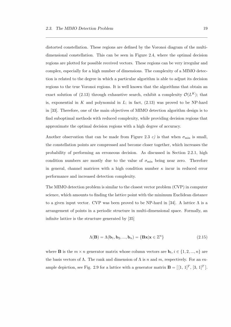
2.3. The MIMO Detection Problem 19
distorted constellation. These regions are defined by the Voronoi diagram of the multi-
dimensional constellation. This can be seen in Figure 2.4, where the optimal decision
regions are plotted for possible received vectors. These regions can be very irregular and
complex, especially for a high number of dimensions. The complexity of a MIMO detec-
tion is related to the degree in which a particular algorithm is able to adjust its decision
regions to the true Voronoi regions. It is well known that the algorithms that obtain an
exact solution of (2.13) through exhaustive search, exhibit a complexity O(LK); that
is, exponential in K and polynomial in L; in fact, (2.13) was proved to be NP-hard
in [33]. Therefore, one of the main objectives of MIMO detection algorithm design is to
find suboptimal methods with reduced complexity, while providing decision regions that
approximate the optimal decision regions with a high degree of accuracy.
Another observation that can be made from Figure 2.3 c) is that when σmin is small,
the constellation points are compressed and become closer together, which increases the
probability of performing an erroneous decision. As discussed in Section 2.2.1, high
condition numbers are mostly due to the value of σmin being near zero. Therefore
in general, channel matrices with a high condition number κ incur in reduced error
performance and increased detection complexity.
The MIMO detection problem is similar to the closest vector problem (CVP) in computer
science, which amounts to finding the lattice point with the minimum Euclidean distance
to a given input vector. CVP was been proved to be NP-hard in [34]. A lattice Λ is a
arrangement of points in a periodic structure in multi-dimensional space. Formally, an
infinite lattice is the structure generated by [35]
Λ(B) = Λ(b1,b2, ...,bn) = {Bx|x ∈ Zn} (2.15)
where B is the m× n generator matrix whose column vectors are bi, i ∈ {1, 2, ..., n} are
the basis vectors of Λ. The rank and dimension of Λ is n and m, respectively. For an ex-
ample depiction, see Fig. 2.9 for a lattice with a generator matrix B = [ [1, 1]T , [3, 1]T ].

2.4. Conventional MIMO Detection algorithms 20
In the context of MIMO detection, the basis vectors correspond to the column vectors
of the channel matrix H, however, the lattices encountered are finite, which can present
problems in certain cases [36].
2.4 Conventional MIMO Detection algorithms
This section provides a review of the most common ‘conventional’ MIMO detection algo-
rithms. These detection techniques are usually associated with small-to-medium MIMO
sizes (from approximately 2× 2 through 20× 20 antennas), and are the counterparts of
the large MIMO detection algorithms, which will be discussed in Section 2.5. A charac-
teristic of conventional MIMO detection techniques is that they suffer from an apparent
tradeoff between error performance and computational complexity [37], as will be dis-
cussed in this section. Conventional MIMO detection techniques have been extensively
studied, a concise tutorial of how they work can be found in [10].
2.4.1 Optimal Detection Methods
ML Detection
As discussed previously, using the ML expression (2.13), the solution with the lowest
possible error probability can be found through exhaustive search among all LK possi-
ble transmit vectors for the one that provides the minimum value of the cost function.
Although this is only practical for small MIMO systems, the algorithm is highly paral-
lisable.
Sphere Decoder
An approach that reduces complexity compared to the full-search ML detector, while still
providing optimum ML error performance is the sphere decoder (SD). The algorithm
was first described by Fincke and Pohst [38], [39] and applied to fading channels by

2.4. Conventional MIMO Detection algorithms 21
Figure 2.5: Conceptual diagram of the sphere decoder algorithm of a 4×4 MIMO systemwith 4-ABPSK modulation with constellation points {-3,-1,1,3}; R denotes the radiusof the hypersphere.
Viterbo and Boutros [40]. An improved, less complex version was developed through
the use of the Schnorr-Euchner (SE) enumeration [41], [35].
The algorithm works by representing the problem by a tree search, where each layer
represents the possible values of the elements of x. Starting from an initial node, which
could be obtained from a ZF decision, the algorithm then searches depth-first in a pre-
defined fashion until it encounters a leaf node. It keeps track of the shortest distance R
found so far of the leaf nodes encountered to the received vector as the search traverses
the tree. The reduction in complexity is the result of skipping the search (pruning) for
tree branches for nodes whose cumulative distance exceeds R. A conceptual diagram of
the SD algorithm is found in Fig. 2.5, for a 4×4 MIMO system with 4-ABPSK modula-
tion with constelation points {−3,−1, 1, 3}. The red nodes and branches indicate those
who would not be visited because their parent node exceeds R. A detailed algorithm
can be found in [35].
The average complexity of the Fincke-Pohst SD was found in [9] to be roughly cubic
in K for moderate-to-high SNRs, however, the complexity is still exponential for low
SNRs. Therefore, a disadvantage of the SD algorithm is that its complexity varies with
the SNR. Fig. 2.6 shows an example algorithm running time vs. SNR for the Fincke-
Pohst and Schnorr-Euchner variants of the SD algorithm. From the figure, the decrease
in complexity is evident as the SNR increases. Furthermore, it can be observed that the
running time for the Schnorr-Euchner approach is roughly half of that of its counterpart.

2.4. Conventional MIMO Detection algorithms 22
0 2 4 6 8 10 12 14 16 18
SNR (dB)
0
50
100
150
200
250
Alg
orith
m r
unni
ng ti
me
(sec
)
Fincke-Pohst SDSchnorr-Euchner SD
Figure 2.6: Example sphere decoding algorithm running time vs. SNR for the Fincke-Pohst and Schnorr-Euchner variants.
The fixed-complexity sphere decoder (FCSD) [42] is based on SD, it performs full search
for the top specified layers of the tree, and uses a decision feedback equaliser (DFE)
for the rest of the layers. FCSD exhibits fixed complexity throughout the SNR range,
however, it comes at the cost of losing BER optimality, and it is still too complex when
the MIMO size is large [23].
The SD algorithm can be modified to output soft detection decisions, as in the list
sphere decoder (LSD) [43] for use in forward error correction (FEC) coded systems. Soft
decisions are obtained through the log-likelihood ratio (LLR) [44]
L(bi|y) = log
(P(bi = 1)|yP(bi = 0)|y
)
= log
∑
x:bi(x)=1
exp(−σ−2
v ‖y −Hx‖2)
∑x:bi(x)=0
exp(−σ−2
v ‖y −Hx‖2) , i ∈ [1,K log2L]
(2.16)
where the notation bi , i ∈ [1,K log2L] refers to the i-th bit contained in the transmitted
vector x, and the notation (x : bi(x) = a) is the set of all vectors x for which bi = a.
The problem with this approach, is that the number of terms to be summed are 2K log2L,

2.4. Conventional MIMO Detection algorithms 23
which makes it feasible only when there are a small number of UTs.
An approximation of (2.16) consists on performing the summations over a smaller subset
of vectors, and is the principle of the LSD, where the subset V of vectors considered
are only the ones that lie within the hypersphere defined by its radius R. While this
approach is less complex than the full search approach in (2.16), it still incurs in increased
complexity compared to the hard decision SD, since the radius R needs to be kept
large enough so that V contains a large number of vectors in order to obtain a close
approximation to the true LLR.
Approximate ML BER
Due to its error performance optimality, the ML BER serves as the standard to which
other detectors are evaluated in their error rate results. Unfortunately, an analytical
closed form expression for the ML BER is not available. However, a useful approximation
exists based on the pairwise error probability (PEP), which is the probability that the
estimated symbol xk is erroneously detected, therefore xk 6= xk (see (2.34)); and for
quadrature phase shift keying (QPSK), the ML BER approximation is given by [45]
PML ≈ Q (√αML · γo) , (2.17)
where Q(·) is the Q-function. When the channel is i.i.d. complex Gaussian, αML is a
chi-square (X 2)-distributed random variable with 2M DoF.
In order to observe the tightness of the BER approximation in (2.17) to the true BER
of an ML detector, Fig. 2.7 compares the ML BER obtained from a SD against (2.17)
for MIMO sizes of 6 × 6, 8 × 8, 10 × 10, and 12 × 12 antennas. From the figure, it
can be observed that the ML and approximate ML curves become closer as the SNR
grows. Furthermore, the approximation becomes tighter as the MIMO size increases.
This approximation will be useful for the BER analysis in Chapter 4.

2.4. Conventional MIMO Detection algorithms 24
0 5 10 15
Eb/N0 (dB)
10-4
10-3
10-2
10-1
100
Ave
rage
BE
R
6x6 ML8x8 ML10x10 ML12x12 ML6x6 Approx. ML8x8 Approx. ML10x10 Approx. ML12x12 Approx. ML
Figure 2.7: True ML vs. ML approximation in (2.17) for an i.i.d. flat Rayleigh fadingchannel, for different MIMO sizes.
2.4.2 Linear Detection
Linear detection methods, MF, ZF and linear MMSE are the simplest for MIMO. The
ZF equaliser or decorrelator is basically the pseudoinverse of the channel matrix
WZF = H† =(HHH
)−1HH (2.18)
where (·)† and (·)H denote the matrix pseudoinversion operation and the complex con-
jugate transpose operation, respectively. Applying the equaliser WZF to (2.1)
x = H†y = x + H†v = x + v (2.19)
completely removes interference. However, the noise that was uncorrelated in v be-
comes correlated in v. This can severely affect the performance, especially for channel
realisations with an ill-conditioned matrix.
The ZF equaliser ignores noise and is well suited for high SNR scenarios, in contrast, for

2.4. Conventional MIMO Detection algorithms 25
very low SNR, the MF WMF = HH equaliser performs best as it maximises the signal
without regard for interference. When applied to the received signal, the result is
x = WMF y = HHH x + HH v , (2.20)
where it is clear that the recovered signals would suffer substantial interference, unless
HHH closely resembles a diagonal matrix.
The overall optimal linear equaliser is the result of finding the equaliser W that minimises
the mean square error (MSE) [46] [21]
MSE = E[‖Wy − x‖2
](2.21)
the result is the MMSE equaliser and it is given by [21, Sec. 8.3.3]
WMMSE =(HHH + γ−1
o I)−1
HH (2.22)
The MMSE filter takes noise into consideration to provide a balance between interference
and noise.
In the context of detection for large MIMO systems, ZF and MMSE receivers are attrac-
tive because of their relatively low complexity, but the maximum diversity order they
provide when the modulation is complex-valuedb is M −K+ 1 [47], which results in low
error performance when the number of transmit and receive antennas is approximately
equal.
2.4.3 Widely-Linear Processing
In communication networks, widely linear (WL) processing achieves superior perfor-
mance over strictly linear filters when the transmission signal, interference or noise is
bIn the sequel, it will be shown that this is not the case for real-valued or hybrid modulation.

2.4. Conventional MIMO Detection algorithms 26
improper (or second-order noncircular [48]) [49], that is, their pseudo-covariance matrix
is non-vanishing. In other words, it means that for complex random processes, the real
and imaginary components have different second-order statistics.
Examples of proper random processes include the circularly symmetric onesc (such as
AWGN), and multilevel quadrature amplitude modulation (QAM); whereas examples of
improper random processes include rectangular QAM, multilevel ABPSK, and coloured
noise.
For a complex-valued multivariate random variable x = xI + jxQ, where xI = R(x)
and xQ = I(x) are the in-phase and quadrature components, respectively, the pseudo-
covariance matrix J is defined as [21, eq. A.16]
J , E[(x− µ)(x− µ)T ] , (2.23)
where µ = E[x].
Denote y = yI + jyQ, where yI = R(y) and yQ = I(y) to be a linear function of
x. The interest is in finding an estimate x of x, given that y is observed. Since for
improper signals J 6= 0, the covariances of xI and xQ are different, therefore a single
MMSE filter WMMSE cannot be simultaneously optimal for estimating both the in-phase
and quadrature components of x. The solution is to use two distinct complex filters WI
and WQ, for yI and yQ, respectively. Therefore, the estimate of x becomes (e.g. [50])
x = WHI yI + WH
Q yQ (2.24)
= FH1 y + FH
2 y∗ , (2.25)
where F1 = WI + WQ, F2 = WI −WQ, and (·)∗ is the complex conjugate operator.
It is worthwhile noting that when x is proper, WI = WQ, and F2 = 0; consequently,
(2.25) reduces to the strictly linear filter form.
WL processing techniques have been proven useful and relevant to numerous applica-
cA random vector x is circularly symmetric if ejθx has the same distribution as x , for any θ [21].

2.4. Conventional MIMO Detection algorithms 27
tions. Particularly, WL techniques of have been applied in [51], [52], and [24] when
using real-valued transmitted signals, such as binary phase shift keying (BPSK) and
ABPSK, by exploiting their improperness. Furthermore, since Gaussian minimum shift
keying (GMSK) modulation can be approximated by filtered BPSK [53], WL filtering
has proposed for global system for mobile communication (GSM) networks, particularly
for single antenna interference cancellation (SAIC) [54], [55], [53]. Additional applica-
tions are in orthogonal frequency-division multiplexing (OFDM) [56], SISO systems with
adaptive constellations [57], CDMA [58], [59], and in multiple-antenna systems, includ-
ing: V-BLAST spatial multiplexing [24], [60], space-time codes (STC) [61], [62], [55],
and MIMO models [51].
2.4.4 Real-Valued Modulation and ABPSK
A recurring theme in this thesis is the assertion that the use of real-valued modulations
in MU-MIMO increases the spatial diversity of MU-MIMO and consequently allow the
use of low-complexity detectors. As a special case of real constellations, the one used
throughout this work is perhaps the simplest case where there the constellation points
are placed along the real axis, with equal spacing between adjacent points, and these
can be positive or negative; a representation is shown on the right side of Fig. 2.8.
There is, however, an ambiguity regarding the name of this modulation type. Some
authors refer to it as multilevel PAM (M-PAM) (see, e.g. [63], [21], [64], [44]), while
other authors refer to it as multilevel amplitude shift keying (ASK) in [24], and [65]
(where it is also referred to as multiple amplitude modulation (M-AM)). However, ASK
usually denotes another type of modulation where the amplitude of the carrier is used to
represent the digital signal [66], whereas PAM often refers to a modulation scheme that
represents the analog data as the amplitude of a series of regularly-timed pulses [67].
To avoid confusion, we refer to the digital modulation scheme described above as L-ary
amplitude binary-phase shift keying (ABPSK). A depiction of a 4-ABPSK constellation
is shown in Fig. 2.8 (right), and a 16-QAM constellation on the left of the same figure

2.4. Conventional MIMO Detection algorithms 28
Figure 2.8: 16-QAM constellation (left), and 4-ABPSK constellation (right), where adenotes the amplitude factor, I and Q the inline and quadrature axes, respectively.
as reference.
2.4.5 Successive Interference Cancellation
The SIC MIMO detection approach was proposed in [13], where it is named as V-
BLASTd. The algorithm works by estimating one element of the transmit vector at one
time, usually starting with the one with the highest post-equalisation SNR or signal-
to-interference-plus-noise ratio (SINR), then subtracting its effect from the remaining
non-estimated signal and iterating until all elements are detected. The reason for first
detecting the strongest elements is to avoid error propagation, since once an estimation
error is made, all further elements will likely be incorrect as well.
Either ZF or MMSE (referred to as ZF-SIC and MMSE-SIC, respectively) can be used
as the equaliser for SIC, and the detection sequence or ordering can be determined once
for each channel realisation based on the post-equalisation SNR or SINR of each stream,
for ZF-SIC and MMSE-SIC, respectively. Specifically for MMSE-SIC, the stream that
dThis term is also often used to describe the MIMO architecture where individual data streams arecoded and transmitted, which is also the scenario considered in this thesis. However, here the term refersto the detection method.

2.4. Conventional MIMO Detection algorithms 29
should be canceled at each iteration is the one with the highest post-equalisation SINR,
given by [68]
SINRk =σ2x |wMMSE,k hk|2
σ2x
∑k 6=j |wMMSE,k hj |2 + σ2
v ‖wMMSE,k‖2, k ∈ [1,K] , (2.26)
where MMSE, k refers to the k-th row of the equalisation matrix given in (2.22). Sim-
ilarly, for ZF-SIC, the selected stream to be canceled at each iteration is the one with
the highest post-equalisation SNR, which is [68]
SNRk =σ2x
σ2v ‖wZF,k‖2
, k ∈ [1,K] , (2.27)
where wZF,k is the k-th row of the ZF equaliser given in (2.18). It should be noted that
since σ2x and σ2
v do not depend on k, it suffices to choose the index of the row of wZF,k
with the lowest norm, which is the approach used in the original SIC paper [13].
It should be noted that the overall optimal ordering is dependent on the received vector,
but doing this would incur in a high computation cost [68].
The original algorithm by [13] has O(K4) complexity. But by reducing redundant op-
erations, mainly by avoiding performing channel matrix inversion on every iteration,
complexity is reduced to O(K3) in [69] and [70].
The SIC technique provides a good balance between error performance and algorithm
complexity.
2.4.6 Lattice Reduction
In general, ill-conditioned channel matrices are harder to estimate without errors. This is
because typically such matrices have a large orthogonality defect (OD), which is defined
as [11]
δ(B) =ΠKi=1||bi||√
det(BHB), (2.28)

2.4. Conventional MIMO Detection algorithms 30
Figure 2.9: Lattice generated by the basis B = [ [1, 1]T , [3, 1]T ], and the basis afterreduction B = [ [1, 1]T , [−1, 1]T ], which has a lower orthogonality defect.
where B refers to the basis of the lattice, as defined in (2.15)e.
LR techniques can provide a ‘lattice-reduced’ matrix H = HT with a lower OD. T is a
unimodular matrix, i.e. its elements are integers and det(T) = ±1.
Once H has been computed, an equivalent system model is found and detection can
progress using a conventional approach such as ZF, MMSE or SIC
y = Hx + v = HTT−1x + v (2.29)
y = Hz + v , (2.30)
where z = T−1x.
eWe use the notation B to refer to the bases of general lattices, whereas we use H in MU-MIMOcommunication contexts. The main difference is that in MU-MIMO, the lattices encountered are finite.

2.4. Conventional MIMO Detection algorithms 31
To illustrate the lattice reduction approach, Fig. 2.9 depicts a lattice generated by a
basis B = [ [1, 1]T , [3, 1]T ]. As seen from the figure, the basis forms a parallelogram (the
red area) with a relatively high OD (which is 2.24); in comparison, after performing the
lattice reduction, the new reduced basis is B = [ [1, 1]T , [−1, 1]T ] , which is perfectly
orthogonal (the blue area).
Several algorithms exist which provide reduced bases for lattices. Some of the most
common are discussed next.
LLL Reduction
One of the most popular LR techniques is the Lenstra-Lenstra-Lovasz (LLL) algorithm
[71], it is an efficient algorithm that finds a good-quality reduced basis in polynomial
time. The LLL algorithm produces short lattice basis vectors [71] (known as the Lovasz
condition), which is a desireable property for MIMO detection since the lattices involved
are finite. An interesting property of MIMO detection with LLL-assisted reduction is
that it can achieve full spatial diversityf [72], [11].
The average complexity of LLL is known to be polynomial in the dimensions of the
lattice [71], and in the worst case, the complexity is also polynomial if the basis vectors
of the lattices are integer-valued [73]. However, in the context of MIMO detection, the
underlying bases of the lattices are continuous-valued, due to the nature of the wireless
channel fading. Consequently, it is shown in [73] that in the worst-case situations with
extremely ill-conditioned channels, the number of iterations of the LLL algorithm is not
bounded. Nevertheless, the cases when the algorithm suffers from an atypically a large
number of iterations are also extremely rare.
fThe maximum spatial diversity when the transmissions among all the UTs are independent, whichis achieved by the ML detector, is equal to M .

2.4. Conventional MIMO Detection algorithms 32
Figure 2.10: Primal lattice with basis B = [ [1, 1]T , [3, 1]T ], and dual lattice with basisB? = [ [−0.5, 1.5]T , [0.5, −0.5]T ].
Seysen’s Algorithm
An alternative to performing a reduction operation on lattice B (which for MU-MIMO
communications corresponds to the channel matrix H), which is referred to the primal
basis, a reduction can be performed on the dual basis, which can be obtained through
the pseudoinverse of B as [11]
B? = (B†)H = B(BHB
)−1. (2.31)
The primal and dual basis are bi-orthogonal, therefore,
bHl b?k =
1 if l = k ,
0 if l 6= k .
(2.32)

2.4. Conventional MIMO Detection algorithms 33
An illustration of the primal and dual lattices, along with their bases B = [ [1, 1]T , [3, 1]T ]
and B? = [ [−0.5, 1.5]T , [0.5, −0.5]T ], is shown in Fig. 2.10.
MIMO detection using the reduced dual lattice has been found to have better perfor-
mance than LR using the primal basis [74], [72].
Seysen’s algorithm (SA) [75] is a LR technique that simultaneously reduces the primal
and dual bases. Its principle is to determine the unimodular matrix T that minimises
the Seysen’s orthogonality measure [11]
S(B) =
n∑i=1
‖bi‖2‖b?i ‖2 . (2.33)
This expression provides an alternate measure of the degree of orthogonality of the basis
vectors, compared to the orthogonality defect in (2.28), since it considers both the primal
and dual bases. Eq. (2.33) reaches its minimum value of S(B) = n, if and only if the
basis vectors are orthogonal [11].
Element-Based Lattice Reduction
The LR techniques mentioned in the previous sections are concerned with the problem
of finding a reduced basis with a low orthogonality defect. The approach presented
by Zhou and Ma in [12], element-based lattice reduction (ELR) is proposed for large
MIMO detection and attempts to reduce the diagonal elements of the noise covariance
matrix. Their results show better performance and lower complexity than LLL or SA
LR approaches for large MIMO systems. A summary of the principle of their approach
is presented next.
The PEP that symbol xi is detected as an error xi, xi 6= xi for a ZF receiver is given
by [12], for QPSK
P (xi → xi|H) = Q
(√|xi − xi|2
2σ2vCii
), (2.34)

2.4. Conventional MIMO Detection algorithms 34
20 30 40 50 60 70 80 90 100 110 120
Number of antennas M=K
10-4
10-3
10-2
10-1
100
Ave
rage
BE
R
ZFLLLSAELR
Figure 2.11: Uncoded BER performance versus number of antennas when M = K oflattice reduction techniques with QPSK modulation at 20 dB Eb/N0, for 16×16 through128×128 antennas, for a frequency-flat i.i.d. Rayleigh fading channel.
where Cii is the i-th diagonal element of C = (H∗H)−1. From (2.34) it can be seen that
the PEP for the i-th symbol depends on the SNR and on C. To reduce the PEP, the
approach finds a unimodular matrix T that will minimise the PEP of the system with
lattice-reduced H
P (zi → zi|H) = Q
(√|zi − zi|2
2σ2vCii
), (2.35)
where z = T−1x is the transmitted vector in the lattice-reduced domain, zi represents
an erroneously i-th estimated symbol, zi 6= zi, H = HT and Cii is the i-th diagonal
element of C = T−1C(T−1
)H.
Since finding an optimal form of T is difficult, a sub-optimal iterative algorithm is
presented in [12].

2.4. Conventional MIMO Detection algorithms 35
LR Simulation Results
Computer simulation results to evaluate the BER performance of LR with LLL, SA and
ELR techniques were performed for different numbers of antennas; from 16×16 through
128×128, for 20 dB Eb/N0 and QPSK modulation in a flat block fading i.i.d. Rayleigh
channel. Figure 2.11 shows the results; from these it is observed that ELR exhibits
the best performance, followed by SA, and lastly by LLL. Furthermore, it is seen that
the BER performance of all three approaches deteriorates as the number of antennas is
incremented; to the point that for 128× 128 MIMO, the BER is close to that of ZF.
From the previous results, it can be concluded that LR techniques are not suitable for
when the MIMO size is large; including the ELR approach, even though it is advocated
as a large MIMO approach in [12].
2.4.7 Semidefinite Relaxation
The SDR approach applies convex optimisation techiques for MIMO detection; it can
obtain a near-optimal solution while experiencing a complexity of O(K3.5) [14], [76].
In the SDR technique, the objective function in (2.13) is re-written into a quadratic
optimisation problem where one constraint is non-convex [14]. SDR then ”relaxes” this
constraint so that the resulting form is tractable. Specifically, by representing the MIMO
model (2.1) in its real form as
y = Hx + v , (2.36)
where
y =
R(y)
I(y)
, H =
R(H) −I(H)
I(H) R(H)
, x =
R(x)
I(x)
, v =
R(v)
I(v)
, (2.37)

2.4. Conventional MIMO Detection algorithms 36
whose dimensions are 2M × 1, 2M × 2K, 2K × 1, and 2M × 1, respectively, then, for
QPSK, (2.13) can be represented as
x = arg minx∈{±1}2K
xTLx = arg minx∈{±1}2K
tr(LX) , (2.38)
where
L =
HT H −HTy
−yH 0
, x =
x
1
, X = xxT , x2k = 1 , k ∈ [1,K] . (2.39)
If the alphabet constraint is removed, the optimisation problem is then
minx∈R2K
tr(LX)
s.t. X � 0 , rank(X) = 1 ,
(2.40)
where the objective function and the first constraint are convex functions; however, the
rank constraint is not convex [14]. Consequently, the second constraint can be dropped,
and the problem becomes
minx∈R2K
tr(LX)
s.t. X � 0 ,
(2.41)
where X is relaxed, from the restriction of having unitary rank, to just being positive
semi-definite. The problem in (2.41) can then be solved efficiently using interior point
methods [77], which are algorithms used to solve convex optimisation problems and
feature polynomial complexity, even in the worst case.
A comparison of the SDR detection technique to other baselines is shown in Fig. 2.12, for
a 4× 4 MIMO system with QPSK modulation. From the figure, it can be observed that
the BER of SDR is very close to that of ML, and much better than the other baselines.
However, one disadvantage of SDR is that it is not straightforward to implement it for

2.4. Conventional MIMO Detection algorithms 37
0 2 4 6 8 10 12 14 16 18 20
Eb/N0 (dB)
10-3
10-2
10-1
100
Ave
rage
BE
R
ZFLLL-ZFMMSE-SICSDRML
Figure 2.12: BER vs. Eb/N0 plot for an uncoded 4× 4 MIMO with QPSK modulationfor SDR and other other detection techniques. Fading channel is frequency-flat i.i.d.Rayleigh.
higher modulation orders, mainly the condition that x2k = 1 is not present, and the lack
of that condition complicates the optimisation process. Nevertheless, SDR algorithms
for multilevel phase shift keying (M-PSK) [78] and QAM (see, e.g. [79], [80]) have been
presented in the MIMO detection literature.
2.4.8 Comparison of Conventional Detection Methods
Some of the most common conventional approaches have been discussed in the previous
subsections. This subsection discusses how they compare to one another in two main
metrics: error performance, and computational complexity. To this end, a plot of the av-
erage BER vs. the algorithm running time during computer simulations using Matlab is
presented in Fig. 2.13g. The algorithms that are compared are ZF, MMSE, MMSE-SIC,
LLL-LR, SDR and the Schnorr-Euchner SD, for QPSK modulation and 12 dB Eb/N0
gIt is expected that the actual algorithm running time in real devices would be different to thosepresented here, due to the underlying hardware. However, the plots provide a rough indicative of thealgorithm complexity; and more importantly, helps highlight the tradeoff between error performance andcomplexity

2.4. Conventional MIMO Detection algorithms 38
100 101 102 103 104
Algorithm running time (s)
10-5
10-4
10-3
10-2
10-1
Ave
rage
BE
R
ZFMMSEMMSE-SICLLL-LRSDSDR
8x8
4x4
Figure 2.13: BER vs. algorithm running time whilst using Matlab of conventional MIMOdetection algorithms for QPSK modulation and 12 dB Eb/N0 for a flat i.i.d. Rayleighfading channel. The left point of each segment shows the results for 4× 4 MIMO, whilethe right corresponds to 8× 8 MIMO.The results are for uncoded systems.
which we believe to be a reasonable operating SNR. For each detection method, simula-
tions were run for two different MIMO sizes, and are plotted in the figure as segments,
where the left and right points of each segment correspond to 4× 4 and 8× 8 antennas,
respectively. The intention of this plot is to show how each algorithm performs in terms
of error performance and complexity, and how these metrics change with the MIMO
size. The figure shows a commonly-discussed theme in this section: an apparent trade-
off exists for conventional MIMO detection algorithms in terms of error performance
and complexity. For instance, ZF and MMSE experience low complexity, but produce
unreliable estimates. On the other extreme, SDR and SD have excellent error perfor-
mance, but also suffer from high complexity. Furthermore, the results also show that
the SIC approach offers a good compromise in detection reliability and complexity, and
is a suitable candidate for MIMO detection.
Aside from their error performance and complexity, each detection algorithm has its own
traits and characteristics, and as a concise summary, these are presented in Table 2.1.

2.4. Conventional MIMO Detection algorithms 39
The most common detection approaches were presented, although it should be noted
that many other MIMO detection techniques exist, such as block-iterative generalised
decision feedback equaliser (BI-GDFE) [81], approaches using Markov chain Monte Carlo
(MCMC) [82], Gibbs sampling [83], partial marginalisation [44], and recently proposed
approaches, such as the LR-based [84], the massive MIMO detection approach in [85],
the branch and bound tree search in [86], and those based on machine learning [87], [88].
Table 2.1: Summary of conventional detection methods.
Detector Characteristics Advantages Disadvantages
Maximumlikelihood
Exhaustive search Optimal errorperformance
Exponential complexity
LinearZF/MMSE
Matrix inversion Simple, lowcomplexity
Low error performance
SIC(V-BLAST)
Layered processingwith channelmatrix ordering
Good performanceand complexitytradeoff
Error performance doesnot improve with theMIMO size
Latticereduction
Reduced basis ofchannel matrix
Basis calculationdone once perchannel realisation
Error performancedegrades with the MIMOsize
Semidefiniterelaxation
Approximationusing convexoptimisation
Near optimal errorperformance
High complexity, notstraightforwardimplementation for highmodulation orders
Spheredecoder
Performs a treesearch, ignoresnodes outsidehypersphere
Optimal errorperformance
High and variablecomplexity
Fixedcomplexityspheredecoder
Full search for toplayers of tree, DFEfor lower layers
Good errorperformance,parallel structure,fixed complexity
Loses optimality vs. SD,high complexity

2.5. Large MIMO Detection Algorithms 40
2.5 Large MIMO Detection Algorithms
Large MIMO detection algorithms are a new class of detection techniques, suited when
the MIMO sizes are large (roughly 40 × 40 or larger). These algorithms have very low
complexity and one of their characteristics is that they can experience large system
behaviour (LSB), which refers to the fact that their error performance improves with
the MIMO size. For MIMO systems with a large number of antennas (approximately
100 × 100 or larger), they exhibit near-optimal reliability. However, they exhibit poor
error performance in small MIMO systems, and unfortunately, they generally only work
well for small order modulations, such as BPSK or QPSK; for 16-ary QAM or higher
modulation orders they either offer poor results, are not easily implementable, or become
too complex (e.g. [89], [90]).
Some of the most common large MIMO detection algorithms are discussed next; useful
references include [23] and [19].
2.5.1 Random Step Methods
Likelihood Ascent Search
LAS is a heuristic algorithm and one of the simplest techniques applicable to large
MIMO detection that can approach near-optimal performance when using low-order
modulation. LAS is based on the Hopfield neural network and was initially developed
for image restoration [91]. It was applied to detection algorithms for code division
multiple access (CDMA) and large MIMO in [15], where results are shown for up to
MIMO sizes of 600× 600 with BPSK modulation.
The pseudocode of the LAS algorithm is depicted in Algorithm 1. It starts by obtaining
an initial estimate, usually through a low-complexity linear approach (ZF, MF, MMSE).
It searches among its neighbour vectors for one with the best cost function. If it finds
one, it is chosen as a candidate vector xc and the search is repeated until all of its

2.5. Large MIMO Detection Algorithms 41
Figure 2.14: Conceptual diagram of LAS algorithm. Starting from the initial vector, thealgorithm searches among its neighbours for those are closer to the received vector.
neighbours have a worse cost function. At this point, the search stops and the candidate
vector xc is selected as the solution. The LAS algorithm outputs hard decisions. A
conceptual diagram of the LAS algorithm is depicted in Fig. 2.14.
The algorithm is ususally presented for BPSK modulation, but it is straightforward for
implementation for L-ary QAM modulations, which implies representing the candidate
vectors xc in their binary form bc ∈ {−1,+1}Klog2(L) [92]. The definition of the neigh-
bourhood can vary and defines the different types of LAS algorithms. A discussion of
these types can be found in [93]. The usual definition of the neighbourhood is the set
of vectors U(bc) which differ from bc on one bit; the cardinality of the neighbour set is
|U(bc)| = Klog2(L).
Equation (2.13) can be used as a cost function, but alternatively, the gradient update

2.5. Large MIMO Detection Algorithms 42
Algorithm 1 Likelihood ascent search
1: procedure LAS2: candidateVector← Obtain initial vector via linear method (ZF, MF, MMSE)3: bestDistance← Compute distance of initial vector4: search:5: neighV ectors← Find neighbour vectors of candidateVector6: neighDistances← Compute distances of all neighVectors7: shortestNeighDist← Shortest distance among neighDistances8: if shortestNeighDist < bestDistance then9: candidateV ector ← Neighbour vector that has shortestNeighDist
10: bestDistance← shortestNeighDist11: goto search.12: else13: Output ← candidateV ector14: end if15: end16: end procedure
Figure 2.15: Example case where the LAS algorithm stops at a local, rather than globalminimum.
function described in [15] is a more efficient way and a key for the algorithm to have low
complexity, this is because the there is usually a 1 bit difference between the candidate
vector and each of its neighbour vectors. Therefore, it is not necessary to fully compute
(2.13) for each candidate vector, but only those computations that are affected by the
one-bit difference, therefore avoiding redundant operations [93].
The LAS algorithm will iterate starting from an initial vector until it reaches a minimum
in the cost function. It can be the global minimum, in which case the ML solution has
been found, or a local minimum, which results in some bits to be erroneous. For a

2.5. Large MIMO Detection Algorithms 43
given channel realisation and received vector, only one global minimum exists (the ML
solution), but zero or many local minima are possible. As an example of a case where
the algorithm does not converge to the ML solution, consider the scenario in Fig. 2.15,
which shows a constellation that has been distorted by the MIMO channel, as described
in Section 2.3. In the figure, the distance from the received vector to the candidate
vector is shorter than to all the neighbour vectors, which causes the algorithm to reach
its stopping condition. Therefore, the green dot is a local minimum, while the red is the
global minimum.
Aside from the complexity of finding the initial vector, the complexity per bit is O(MK)
for the LAS algorithm [15]. The complexity and error performance of LAS are very
sensitive to the initial vector. For L > 4 in a fully-loaded scenario, our simulations show
(the results are presented in Fig. 2.17) that ZF-LAS (LAS with a ZF initial solution) does
not converge to the optimal solution (MMSE-LAS does approach optimal performance
for L = 4).
As with most detection algorithms that perform search functions, e.g. SD, the complexity
of LAS varies with the SNR. This is because as the SNR increases, the estimation
accuracy of the initial vector is improved, thus the algorithm converges more rapidly to
a local (or global) minimum.
A plot of the average BER vs. Eb/N0 of uncoded MIMO systems of different sizes; from
16 × 16 up to 128 × 128 is shown in Fig. 2.16, where the modulation is BPSK. From
the figure, it is evident that the performance improves with the MIMO size (exhibits
LSB); the curves become closer to the single-input single-output (SISO) AWGN curve,
which can be considered as the lower bound for very large MIMO systems. Since LAS
is a heuristic algorithms, its analysis can be difficult, and the reason why the algorithm
converges (or the conditions in which it converges) to near-optimal BER are not entirely
clear, although an analysis in the large system limit and for BPSK modulation can be
found in [94].
However, as with most large MIMO detection algorithms, the performance is not scalable

2.5. Large MIMO Detection Algorithms 44
0 5 10 15 20 25 30
Eb/N0 (dB)
10-6
10-5
10-4
10-3
10-2
10-1
100
Ave
rage
BE
R
16x16 ZF-LAS32x32 ZF-LAS64x64 ZF-LAS128x128 ZF-LASSISO AWGN
Figure 2.16: Average BER vs. Eb/N0 of uncoded BPSK-modulated MIMO with LASdetection for different system sizes, for a flat i.i.d. Rayleigh channel. The figure showsthat the error performance improves with the MIMO size.
with the modulation order. To see this, the BER vs. Eb/No plot of ZF-LAS and MMSE-
LAS (LAS algorithm using an MMSE initial solution) using QPSK is shown in Fig. 2.17.
From the figure, it can be observed that ZF-LAS does not improve with the MIMO size,
although MMSE-LAS does converge towards the ML bound as the number of antennas
increases. For higher order modulations, e.g. 16-QAM, although not presented here, our
simulations showed that neither ZF-LAS nor MMSE-LAS converge towards the optimal
BER as the MIMO size increases.
Authors have proposed LAS algorithm variants. The multiple output selection LAS [95]
performs multiple LAS searches, each starting from a different initial solution, obtained
from MF, ZF, and MMSE, and selecting the best solution; while the multistage LAS
[96] increases the neighbourhood definition when a minimum solution is encountered,
therefore increasing the probability of finding a new minimum, in case the one previously
encountered was not the global solutions.

2.5. Large MIMO Detection Algorithms 45
0 5 10 15 20 25 30
Eb/N0 (dB)
10-4
10-3
10-2
10-1
100
Ave
rage
BE
R
16x16 ZF-LAS32x32 ZF-LAS64x64 ZF-LAS128x128 ZF-LAS16x16 MMSE-LAS32x32 MMSE-LAS64x64 MMSE-LAS128x128 MMSE-LASSISO AWGN
Figure 2.17: Uncoded BER performance versus Eb/N0 of ZF-LAS and MMSE-LASwith QPSK modulation for different numbers of antennas. It is shown that MMSE-LAS converges to near-optimal performance as the number of antennas increases, whileZF-LAS does not. The fading channel is frequency-flat i.i.d. Rayleigh.
Tabu Search
The LAS algorithm studied in the previous subsection, although simple and efficient,
lacks a way to escape local minima that prevents it to find the ML solution. The TS
algorithm [97], [98] operates on the same principle as LAS, but the search is able to
move towards neighbouring points with a worse metric, which prevents it from getting
stuck at local minimum points. Since this behaviour may cause the search to go into a
loop, the algorithm keeps a tabu list of moves that have already been made in the past
for certain number of iterations, which is called tabu period. If the search encounters
a potential move that is kept in the tabu list, it prohibits that move (hence the name
‘tabu’) and the search progresses in another direction.
Although TS solves the problem of LAS stopping at local minima, it creates new issues,
such as increased search complexity and algorithm complexity. The optimal stopping
condition is difficult to establish, since the algorithm is unable to determine for certain
if the ML solution has been found. A stopping condition that is too strict may keep the

2.5. Large MIMO Detection Algorithms 46
0 2 4 6 8 10 12 14 16
Eb/N0 (dB)
10-4
10-3
10-2
10-1
100
Ave
rage
BE
R
16x16 MMSE-LAS32x32 MMSE-LAS64x64 MMSE-LAS16x16 MMSE-TS32x32 MMSE-TS64x64 MMSE-TSSISO AWGN
Figure 2.18: Average BER vs. Eb/N0 of MMSE-TS vs. MMSE-LAS for different MIMOsizes. The results are for uncoded systems with a flat i.i.d. Rayleigh channel.
search running even though the ML solution has already been found (thus increasing
the complexity) and a relaxed stopping condition may stop the search before reaching
the ML solution (this case would increase the number of errors).
Due to its ability to escape local minima, TS exhibits improved error performance over
LAS, at the cost of increased algorithm complexity. This can be seen in Fig. 2.18, where
the BER vs. Eb/N0 of MMSE-LAS and MMSE-TS (TS with an MMSE initial solution)
is plotted for different MIMO sizes and QPSK modulation. From the figure, it can be
observed that MMSE-TS offers near-optimal BER for 64× 64 MIMO.
Several variants of TS have been presented in the literature, namely, the reactive TS
approach [99], [92], which is able to adjust the algorithm parameters as the search
progresses, and allows it to specify a dynamic stopping criteria; additionally, the random-
restart reactive TS [100] and the layered TS [90] enable the TS algorithm for 16-QAM
and 64-QAM modulations, albeit at the cost of a significant increase in complexity.

2.5. Large MIMO Detection Algorithms 47
0 5 10 15
Eb/N0 (dB)
10-6
10-5
10-4
10-3
10-2
10-1
100
Ave
rage
BE
R
PDA
16x1632x3264x64128x128SISO AWGN
0 5 10 15
Eb/N0 (dB)
10-6
10-5
10-4
10-3
10-2
10-1
100
Ave
rage
BE
R
BP
16x1632x3264x64128x128SISO AWGN
Figure 2.19: BER vs. Eb/N0 for PDA (5 iterations) and damped BP (20 iterations, witha 0.4 damping factor) for different MIMO sizes with QPSK modulation, for uncodedsystems with a frequency-flat Rayleigh fading channel.
2.5.2 Methods Using Gaussian Approximation of Interference
Other types of large MIMO detection algorithms are those who model the co-channel
interference as a normal distribution. These include the damped BP [18] and the PDA
[19] detection approaches. For example, the damped BP algorithm models the MIMO
equation (2.1) as
ym = hmkxk +K∑
j=1,j 6=khmjxj + vm︸ ︷︷ ︸
Interference, zm
, k ∈ [1,K] , m ∈ [1,M ] , (2.42)
where the interference term is modeled as CN (µzm , σ2zm). As the number of antennas
increases, the Gaussian approximation of interference (GAI) modeling approximation
becomes more accurate because of the central limit theorem (CLT). The mean and

2.5. Large MIMO Detection Algorithms 48
variance of the interference are
µzm =K∑
j=1,j 6=khmjE(xj) , (2.43)
σ2zm =
K∑j=1,j 6=k
|hmj |2var(xj) + σ2v , (2.44)
for BPSK modulationh, and denoting P(xk) to be the probability of xk = 1, we have [101]
E(xj) = 2P(xj)− 1 , (2.45)
var(xj) = 4P(xj)(1− P(xj)) . (2.46)
Due to the Gaussian approximation,
P(ym|xk ,H) ∝ exp
(−1
σ2zm
(ym − hmkxk − µzm)∗(ym − hmkxk − µzm)
), (2.47)
thus the LLR of the k-th transmitted symbol at the m-th receive antenna is
Lkm , logP(ym|H , xk = +1)
P(ym|H , xk = −1)(2.48)
=4
σ2zm
R(h∗mk(ym − µzm)) . (2.49)
By adding the LLRs of all the observations at the M receive antennas, we obtain the a
posteriori probability (APP) of the k-th symbol as
P(xk|y) =
exp
(M∑
l=1,l 6=kLkl
)
1− exp
(M∑
l=1,l 6=kLkl
) . (2.50)
The algorithm then iterates, and updates the a priori probabilities P(xk) in (2.43)-
(2.46), with the APPs P(xk|y) obtained in (2.5.2). However, in order to improve BER
hThe algorithm can be used for QPSK straightforwardly, by representing the MIMO equation in itsreal form, as in (2.37).

2.5. Large MIMO Detection Algorithms 49
performance, the old probabilities should not be completely replaced by the new ones,
but ‘damped’ through a weighted average given by
P(xk)+ = αmP(xk) + (1− αm)P(xk|y) , (2.51)
where P(xk)+ refers to the probabilities to be used in the next iteration, and αm is the
damping factor. A value of αm = 0.4 that was shown to produce good results in [18].
The BP algorithm runs for a specified number of iterations. Upon its completion, the
estimate of the transmitted symbols can be obtained by
xk = sgn
(M∑l=1
Lkl
), (2.52)
where sgn(·) refers to the sign function.
The PDA approach is similar to BP in that both are iterative algorithms, where in
each posterior probabilities are computed and used as the prior probabilities in the next
iteration (see [19]). But more importantly, both make use of GAI.
The main difference between damped BP and PDA is that the former models the inter-
ference as a scalar in (2.42) and the latter as a vector, as
y = hkxk +
K∑j=1,j 6=k
hjxj + v︸ ︷︷ ︸Interference, z
. (2.53)
The PDA per-symbol complexity is O(K2), and the damped BP complexity is O(K) [19].
The BER of PDA and damped BP can be seen in Fig. 2.19. It can be observed from
the figure that damped BP achieves better results, which become very close to the lower
bound for 128×128 antennas.
Similar to other large MIMO approaches, PDA and damped BP, extensions to higher
order modulations is not straightforward.

2.6. Summary 50
20 30 40 50 60 70 80 90 100 110 120
M=K Number of antennas
10-6
10-5
10-4
10-3
10-2
10-1
100
Ave
rage
BE
R
ZF-LASMMSE-LASPDABPSISO AWGN
Figure 2.20: BER vs. number of antennas (with M = K) of large MIMO detectionalgorithms for QPSK modulation and 10 dB Eb/N0, with a flat i.i.d. Rayleigh fadingchannel, for uncoded systems.
2.5.3 Comparison of Large MIMO Detection Approaches
Some of the most common large MIMO detection techniques have been discussed, and in
general, their error performance improves with the MIMO size (exhibit LSB) when using
low-order modulation orders. However, as the number of antennas increases, their rate
of convergence towards the ML lower bound is different for each large MIMO detection
approach. This can be observed in Fig. 2.20, where the curves of the average BER are
plotted against the MIMO size, for 10 dB Eb/N0 and QPSK modulation. The figure
shows that damped BP has the fastest convergence, followed by PDA and MMSE-LAS.
However, as discussed previously, ZF-LAS does not converge towards the optimal BER
when using QPSK modulation.
2.6 Summary
This section has discussed the preliminaries and state-of-the-art of MU-MIMO detection.
For a low spatial loading (M � K), low-complexity detection methods, such as MF and

2.6. Summary 51
ZF become near optimal and MU-MIMO detection is relatively easy. However, in user-
dense networks with a high spatial loading (M ≈ K), there are significant challenges in
the form of detection reliability and complexity. It was argued that this phenomenon is
mainly due to the condition number κ of the channel matrix; for well-conditioned matri-
ces, ZF becomes near optimal, but ill-conditioned matrices result in increase detection
errors and computational complexity. The Marcenko-Pastur law explains the relation-
ship between the condition number κ and the MIMO channel matrix dimensions, which
ultimately affect the MIMO detection performance.
Furthermore, two categories of detection methods were presented: conventional MIMO
detection approaches, and large MIMO detection approaches. First, for conventional
MIMO techniques, an apparent complexity-reliability tradeoff exists, and this was ex-
plained by the optimal MIMO detection regions, which become increasingly complex
with the number of dimensions, or MIMO size. The relationship between the error per-
formance and complexity of the conventional detection techniques can be explained geo-
metrically, by observing how closely the decision regions of a particular method emulate
the optimal ML decision regions. And second, for large MIMO detection approaches, the
error performance improves with the MIMO size, which eventually become near-optimal
for large MIMO sizes. However, for medium-sized MU-MIMO, limited detection op-
tions exist, as conventional detection algorithms become too complex, and large MIMO
detection approaches offer low error performance.
Conventional and large MIMO detection techniques have their own drawbacks; gener-
ally speaking, conventional techniques are not scalable with the MIMO size, while the
large MIMO approaches are not scalable with the modulation orderi. This creates an
opportunity for detection approaches that may offer increased scalability in both the
MIMO size and modulation order. The proposed techniques that will be presented in
Chapter 3 and 4 are an attempt to do just that, however, a different approach is taken
iNote that some adaptations of some techniques such as TS [90] and BP [89] are extendable for highermodulation orders, at the cost however, of a large complexity increase, therefore no longer suitable forlarge MIMO systems.

2.6. Summary 52
by also involving the transmitters, where the detection reliability and performance are
improved through modulation design.

Chapter 3Real-Modulated Dense MU-MIMO
Communications
In densely populated areas, the number of transmit antennas can be equal or higher
than the number of service antennas. These systems are referred to as fully-loaded
or over-loaded MU-MIMO systems, for which linear receivers such as ZF and linear
MMSE yield very poor performance. In contrast, non-linear receivers [19] lead to high
computational complexity, especially in over-loaded scenarios. Detection approaches
exist that are applicable to over-loaded MIMO, notably, the generalized SD [102] offers
excellent performance, however, at the cost of prohibitive complexity, even higher than
the conventional SD. Another approach is the layered tabu search technique in [103];
it offers good error performance, but it is also hindered by high complexity. Therefore,
the implementation of current detection techniques becomes challenging in large MIMO
systems, notably for certain emerging wireless applications such as large-scale internet
of things (IoT) networks [104], which are very demanding in terms of both the large
number of connected IoT devices and high link reliability.
Buzzi et al. applied a widely linear filter along with ABPSK modulation to improve sig-
nal detection in fully- and over-loaded (small) MIMO systems [24]. WL filters typically
53

3.1. MU-MIMO with Real Constellations 54
Figure 3.1: Block diagram of MU-MIMO with a WLZF-LAS receiver. The FEC, MODand FEC−1 blocks refer to the channel coding, ABPSK modulators and channel decod-ing, respectively.
exhibit superior performance compared with strictly linear filters when the transmitted
signals, interference, or noise are improper, which is the case when real-valued transmis-
sions are used. Widely linear filters were discussed in Section 2.4.3.
In this work, we apply the WL filter derived in [24] (termed WLZF) into fully- and over-
loaded large MU-MIMO systems with real-valued constellations. The main motivation
is that the WLZF receiver has low complexity, similar to that of ZF, with respect to the
MIMO system size even in very large over-loaded scenarios. Specifically, our contribu-
tions include: 1) we find that the spatial diversity of WLZF under Rayleigh fading is
M − K/2 + 1/2 (cf. diversity of ZF is M − K + 1); the diversity expression also allows
us to find the exact SER of WLZF, and the diversity-multiplexing tradeoff that WLZF
exhibits, and 2) we present some interesting results upon applying WLZF as the starting
point for the LAS receiver, because due to the large spatial diversity gain, the algorithm
can quickly converge to a near-optimal decision without the knowledge of noise variance.
3.1 MU-MIMO with Real Constellations
The uplink of a wireless large MU-MIMO communication system is considered, subject
to K ≤ 2M , where the system loading factor is defined as α = K/M . The system model
is the one described in Section 2.1. The block diagram of the proposed approach is shown
in Fig. 3.1, where independent bit streams bk, k ∈ [1,K] which denote the information
bits of each UTs are independently FEC-coded, ABPSK-modulated, transmitted and

3.1. MU-MIMO with Real Constellations 55
passed through the MIMO channel. At the receiver, the multiplexed signals ym, m ∈
[1,M ] are passed through the WLZF equaliser, which removes the interference. A hard
decision is taken for each stream and fed into the LAS post-processing stage, and finally
independently FEC-uncoded. The output are the bit streams bk, which are the estimates
of the information bits bk.
This section will begin by presenting some preliminaries of ZF equalisation, particularly
the approximate outage probabilities, which will be useful for the remaining part of
the section. Then, a simple derivation is presented of the WLZF filter in [24], which
is used for recovering real-valued transmissions. Subsequently, we derive the spatial
diversity order of WLZF, which will be key to finding the approximate system outage
probability, which in turn will allow us to express the diversity-multiplexing tradeoff
of MU-MIMO with real-valued constellations and WLZF equalisation. As a particular
case of real constellations, L-ary ABPSK modulation is used. Then, the exact SER
(and approximate BER) is derived for WLZF with L-ABPSK modulation. Next, to
further increase detection reliability, WLZF-LAS is proposed, which consists of WLZF
equalisation followed by a LAS processing stage, as shown in the block diagram in Fig.
3.1. Finally, computer simulations are presented to evaluate the performance of WLZF
and WLZF-LAS in fully- and over-loaded MU-MIMO with L-ABPSK modulation.
3.1.1 Preliminaries of ZF equalisation
The objective is to find an approach that has comparable complexity with the linear
ZF algorithm whilst offering better error performances. To this end, it is worthwhile to
revisit the ZF algorithm from (2.18), which employs the matrix WZF = (HHH)−1HH
to equalise the MIMO channel
z = WZFy = x + (HHH)−1HHv, (3.1)
therefore every user’s message is individually detected. The complexity of ZF channel
equalisation is O(MK2+K3) [23]. The terms x, and z in (3.1) have 0 mean, and the co-

3.1. MU-MIMO with Real Constellations 56
variance of the signal term is cov(x) = σ2xI, and for the noise term cov
((HHH)−1HHv
)=
σ2v(H
HH)−1, therefore, the post-equalisation SNR for the kth element of z is given by
γk =γo[
(HHH)−1]kk
. (3.2)
The system outage probability, which occurs when at least one data stream out of K in
(3.1) is in outage, is approximately [105]
P(3.1)out = 1− P
(K⋂k=1
{I(zk;xk) ≥
R
K
})(3.3)
= 1−(P(I(zk;xk) ≥
R
K
))K(3.4)
≈ K P(I(zk;xk) <
R
K
)(3.5)
= K P(
log(1 + γk) <R
K
)(3.6)
= K P(γk < 2R/K − 1
)(3.7)
= K Fγk
(2R/K − 1
), (3.8)
where R is the sum rate of all the transmissions by the K UTs, and I(zk;xk) = log(1+γk)
denotes the mutual information between zk, xk, which refers to the kth element of z
and x, respectively. Eq. (3.4) is due to independence of the UT transmissions, and the
approximation at (3.5) is accurate when the outage probabilities are small, (3.7) is found
solving for γo, and (3.8) comes from the definition of FX(x), which is the cumulative
distribution function (CDF).
Assuming H to be an i.i.d. complex Gaussian matrix, (γk)/(γo) is known to be chi-square
distributed with 2(M − K + 1) degrees of freedom, i.e. γk/γo ∼ χ22(M−K+1) [106], [45],
for high SNR the outage probability can be expressed as [21, Eq. (5.66)]
P(3.1)out ≈
K(2R/K − 1)Dcplx
Dcplx!γ−Dcplxo (3.9)

3.1. MU-MIMO with Real Constellations 57
where (R)/(K) is the target data rate of each individual usera, and Dcplx = M −K + 1
is the spatial diversity order. Comparing to the optimal algorithms (e.g. ML) with
diversity order M (or equivalently, 2M degrees of freedom)b, the ZF algorithm is too
suboptimal in terms of degrees of freedom and spatial diversity order, particularly for
the case of M = K (or M ≈ K).
3.1.2 Widely Linear Zero Forcing
In the following, a simple characterization of the filter proposed in [24] (denoted as
WLZF) is presentedc; we then obtain the expression for diversity that it achieves.
The MIMO model equation (2.1) can be written in its real representation as
R(y)
I(y)
=
R(H) −I(H)
I(H) R(H)
︸ ︷︷ ︸
H(R)
R(x)
I(x)
+
R(v)
I(v)
, (3.10)
where R(·) and I(·) are the real and imaginary components, respectively. However,
because the transmit symbols are selected from a real constellation, I(x) = 0, therefore
(3.10) is equivalent to
R(y)
I(y)
=
R(H)
I(H)
[R(x)]
+
R(v)
I(v)
, (3.11)
which can be written in compact form as
y = Hx + v , (3.12)
aHere an equal rate is considered for each UT. As justified in [105], a generalization to unequal rateassignment is immediate, since equal or unequal rate assignments have the same diversity.
bAn independent complex signal contains 2 DoF (the real and imaginary components), but only con-tributes for unitary diversity. This can be seen by representing the complex signal in polar coordinates,where the magnitude component contributes with the diversity, but not the phase component.
cThe derivation of the filter in [24] follows a different path. Here we present what we believe is asimpler derivation, with a clear representation that simplifies its analysis and allows its further extensionto the proposed approach in Chapter 4.

3.1. MU-MIMO with Real Constellations 58
where y, H, x, and v are real-valued and have dimensions 2M × 1, 2M ×K,K × 1, and
2M × 1, respectively. The ZF estimate of the transmitted signal using (3.1) is given
by z = H†y, where (·)† denotes the pseudoinverse. However, it should be noted that it
is not necessary to perform a pseudoinversion on the full channel matrix; therefore, a
better approach is to use (3.12)
z = H†y =
R(H)
I(H)
† y = R(x) + (HHH)−1HH v (3.13)
which is the WLZF approach. The benefits are due to the fact that the equivalent
channel matrix H has half the number of columns that the real representation of the
channel matrix H(R) has, thus making it better conditioned, as discussed in Section
2.2.1. Furthermore, because half the column vectors are removed, up to twice as many
transmit antennas than receive antennas can be used, since when K = 2M , the channel
matrix H becomes square, a fact recognised in [24]; this would make the system over-
loaded but the channel matrix would not be underdetermined. It should be noted that
these terms are not the same: ‘over-loaded’ is with reference to the number of antennas,
and ‘underdetermined’ is an attribute of the channel matrix.
Proposition 3.1. When H is i.i.d. complex Gaussian, the WLZF approach achieves a
diversity of
DWLZF = M − K
2+
1
2. (3.14)
Proof. see Appendix A.
Having derived the spatial diversity expression of WLZF, the approximate outage prob-
ability for WLZF can be obtained in the same way as the for ZF. Following (3.3 - 3.9),
the system outage probability of WLZF with real-valued modulation is approximately
P(3.13)out ≈ K(22R/K − 1)DWLZF
Γ(DWLZF + 1)γ−DWLZFo , (3.15)

3.1. MU-MIMO with Real Constellations 59
where Γ(·) is the gamma function, and DWLZF = M −K/2 + 1/2 is the spatial diversity
achieved by WLZF, obtained from Proposition 3.1. It can be concluded that the use of
real modulations effectively increases the spatial diversity order by (K − 1)/2, without
penalty to the computation complexity. On the other hand, the spatial multiplexing
gain is reduced by K/2, compared to the complex modulation. The outage probability
in (3.15) will be used to determine the diversity-multiplexing tradeoff of WLZF, which
is discussed next.
3.1.3 The Diversity-Multiplexing Tradeoff of WLZF
The diversity-multiplexing tradeoff, as described by Zheng and Tse [107], [21], is a funda-
mental property of communications systems in slow fading channels. It is a simplification
of the outage probability vs. target rate curves in the high-SNR regime. It asserts that a
communication scheme can simultaneously exploit the degrees of freedom and diversity
of the channel, up to a certain amount. Specifically, it states that when the data rate
R(SNR) for a space-time coding scheme scales as
limSNR→∞
R(SNR)
log SNR= GMUX , (3.16)
where GMUX is the multiplexing gain, and when the probability of error Pe(SNR) follows
limSNR→∞
logPe(SNR)
log SNR= −GDIV , (3.17)
where GDIV is the diversity gain, then the the diversity-multiplexing tradeoff curve is
given by GDIV(GMUX). This is because, since GMUX and GDIV both depend on the SNR,
then they also depend on each other.
Corollary 3.1.1. The diversity-multiplexing tradeoff of WLZF is given by
GDIV =
(M − K
2+
1
2
)(1− GMUX
K/2
), GMUX ∈
[0,K
2
](3.18)

3.1. MU-MIMO with Real Constellations 60
Figure 3.2: The diversity-multiplexing tradeoff (Gdiv, Gmux) of WLZF with real modu-lations and ZF with complex modulation.
Proof. From the result in [21, Eq. 9.20], the diversity-multiplexing tradeoff for a parallel
channel with D diversity branches is GDIV = D (1 − GMUX), with GMUX ∈ [0, 1]. By
analogy and substituting the diversity and multiplexing gain achieved by WLZF, it is
straightforward to obtain the DMT of WLZF.
The diversity-multiplexing curve achieved by WLZF is plotted in Fig. 3.2, along with the
DMT curve of ZF. From the figure, it can be seen that the use of real-valued modulated
signals increases the diversity gain (which can be positive even for some cases where
K > M), compared to complex modulations. In exchange, the multiplexing gain of real
signals is halved. This means that WLZF can efficiently exploit the spatial degrees of
freedom at the cost of a loss in modulation efficiency. The use of real constellations
can offer improved performance over complex modulations when using linear receivers
in some scenarios, such as in fully- and over-loaded MU-MIMO without incurring in
additional complexity, since most of the complexity involves the channel matrix inversion.
WLZF can be seen as a way of splitting the in-phase and quadrature components of a
complex stream into two separate real streams; in doing so, twice the number of transmit

3.1. MU-MIMO with Real Constellations 61
antennas are supported. In exchange, the orthogonality that existed in the components
of the complex stream disappears, which results in a slight decrease of 0.5 in diversity.
This is in agreement with the analysis presented in [108], where it was observed that
a complex stream occupies 2 degrees of freedom out of the total 2M available in the
system, but a real stream uses only 1 DoF; thus, by assiging only one real stream per
UT, twice as many UTs accommodated, effectively doubling the number of users served
by the network, at the cost of a diminished throughput efficiency of each user. WLZF
is also consistent with [54], where it is shown that a receiver array with M elements can
suppress 2M−1 rectilinear interferences, effectively supporting 2M real-valued streams.
3.1.4 Analytical Error Rate of WLZF with L-ary ABPSK Modulation
In this section, the exact average SER expression is found for a MIMO system with i.i.d.
Rayleigh fading with D diversity branches, when D is allowed to be fractionald (as is
the case for DWLZF in (3.14) when K is even), using L-ary ABPSK modulation; this
expression will then be used to obtain the approximate BER.
For MU-MIMO with a ZF receiver and BPSK or QPSK modulation, the exact average
BER expression is given in [109, eq. (7)] as
P(BPSK)b =
1
2−√γoπ
Γ(D + 12)
Γ(D)× 2F1
(1
2, D +
1
2;3
2;−γo
), (3.19)
where D is the diversity order, Γ(·) is the Gamma function and 2F1( , ; ; ) is the hyperge-
ometric function. Eq. (3.19) also applies to WLZF with BPSK, by using D = DWLZF.
After ZF or WLZF equalisation the K streams are effectively decoupled and detected
individually, and since all the streams have the same distribution per (3.2), it is sufficient
to analyze the error rate of a single stream to determine the overall MU-MIMO error
rate. Therefore, the approach for finding the average error rate for MU-MIMO with
ZF or WLZF equalisation consists on finding the expected value of the error rate of a
dClosed form error probability expressions for integer-valued D are more common (e.g. [21, Eq. (3.37)]for BPSK / QPSK).

3.1. MU-MIMO with Real Constellations 62
SISO system, averaged over the distribution of the instantaneous SNR γk, which is a
random variable. Using this approach, (which is used in [109] to find (3.19)), the error
probability for L-ary ABPSK can be derived as follows.
The instantaneous SER for a SISO system with L-ABPSK is given by [65, eq. (8.3)]
P(ABPSK)s =
2(L− 1)
LQ
(√6γk
L2 − 1
), (3.20)
where Q(x) is the Q-function defined as 1√2π
∫∞x e−t
2/2 dt. Since γk is a random variable,
the expectation over γk needs to be taken in order to find the average SER, denoted as
P(ABPSK)s
P(ABPSK)s = Eγk
[P(ABPSK)s
](3.21)
=
∫ ∞0P(ABPSK)s f(γk) dγk (3.22)
=
∫ ∞0
2(L− 1)
LΓ(D) γoQ
(√6γk
L2 − 1
) (γkγo
)D−1
e− γkγo dγk (3.23)
=2(L− 1)
LΓ(D)
∫ ∞0
Q
(√6γγoL2 − 1
)γD−1 e−γ dγ (3.24)
where f(·) is the probability distribution function (PDF), and e is the base of the natural
logarithm. The last two steps in are because of the definition γ = γk/γo (note that
E[γk] = γo), where γ ∼ X 2D.
Since the Q function can be written as [109]
Q(x) =1
2− x√
2πΦ
(1
2;3
2;−x
2
2
), (3.25)
where Φ( ; ; ) is the confluent hypergeometric function of the first kind. By substituting

3.1. MU-MIMO with Real Constellations 63
(3.25) into (3.24), the following is obtained
P(ABPSK)s =
2(L− 1)
LΓ(D)
∫ ∞0
(1
2−
√3γγo
π(L2 − 1)Φ
(1
2;3
2;− 3γγo
L2 − 1
))γD−1 e−γ dγ .
(3.26)
Applying identity (7.621.4) from [110] the final exact SER expression is
P(ABPSK)s =
L− 1
L−2(L− 1)
L
√3γo
π(L2 − 1)×
Γ(D + 12)
Γ(D)
× 2F1
(1
2, D +
1
2;3
2;−3γoL2 − 1
).
(3.27)
The average BER can then be approximated by [65, eq. (8.7)]
P(ABPSK)b ' P
(ABPSK)s
log2L, (3.28)
where the notation ‘'’ refers to an asymptotic equality.
As mentioned above, these results are for a general MIMO system using L-ABPSK
modulation with D diversity branches, therefore, by setting D = DWLZF, (3.27) and
(3.28) describe the exact SER and approximate BER, respectively, of L-ary ABPSK-
modulated MU-MIMO with WLZF equalisation.
3.1.5 WLZF-LAS
As was seen in Chapter 2, linear equalisers such as ZF and MMSE are commonly used
as building blocks for more advanced detection techniques; for instance, ZF can be used
as the initial step for the SD. Therefore, we propose to use WLZF as the first stage for
the LAS algorithm, and denote it as WLZF-LAS. A block diagram of MU-MIMO with
WLZF-LAS is shown in Fig. 3.1.
LAS is a heuristic algorithm applicable for large MIMO detection and is able to achieve

3.2. Performance Evaluation and Discussion 64
near-optimal error performance with a complexity per bit of O(MK). LAS was reviewed
in Section 2.5.1, where the algorithm was presented.
The complexity and error performance of LAS are very sensitive to the initial vector.
For m > 4 in fully-loaded scenario, ZF-LAS (LAS with a ZF initial solution) does not
converge to the optimal solution (MMSE-LAS does approach optimal performance for
m = 4). However, by using WLZF as the starting point, and with the reduced-column
channel matrix H, WLZF-LAS is able to find a near-optimal solution without the need
for noise variance knowledge. The results in the next section will show that this is true
even for high modulation orders such as 16-ABPSK, something that the conventional
LAS algorithm is unable to achieve.
3.2 Performance Evaluation and Discussion
Computer simulations were performed to evaluate WLZF and WLZF-LAS in large MU-
MIMO systems with an i.i.d. frequency-flat block Rayleigh fading channel. Results
are presented for a 128×128 fully-loaded case, and for up to 64 × 128e in over-loaded
scenarios, for uncoded and coded systems. The proposed techniques allow even larger
MIMO sizes due to their low complexity. However, the number of streams for which
CSIR estimation can be performed in one channel coherence period limits the number of
UTs (although the channel coherence time could be relatively long for some static or low-
mobility IoT devices). Because the network density is expected to keep increasing [2],
CSIR estimation for a large number of antennas is an active research area and some
promising approaches to this problem have been presented, e.g., pilot reuse [111].
The performance of WLZF has been evaluated for small MIMO systems in [24]. This sec-
tion focuses on large MIMO systems, mainly because of two reasons: 1) the performance
of WLZF improves as the MIMO size increases, given a fixed α (recall that α = K/M),
due to the increased diversity order; and 2) no other approaches (e.g., [103]) seem to be
eRecall that this notation refers to M ×K.

3.2. Performance Evaluation and Discussion 65
0 2 4 6 8 10 12 14 16 18 20
Eb/N0 (dB)
10-4
10-3
10-2
10-1
100
Ave
rage
BE
R
WLZF 16-ASKWLZF 8-ASKWLZF 4-ASKWLZF BPSKZF BPSKZF QPSKZF 128x64 QPSKAWGN 1x1 BPSKWLZF Theory
Figure 3.3: BER vs. Eb/N0 in a fully-loaded system for ZF and WLZF for L = {2, 4},and WLZF for L = {2, 4, 8, 16} with 128×128 antennas. Also includes results for ZF us-ing QPSK with 128×64 antennas. The results are for uncoded systems with a frequency-flat block Rayleigh fading channel.
feasible (as far as the authors are aware) for large over-loaded MIMO systems, due to
their high complexity.
WLZF in fully-loaded uncoded large MU-MIMO The BER vs. Eb/N0 results
are exhibited in Fig. 3.3 for an uncoded fully-loaded scenario with 128×128 antennas
and other supporting cases. The following plots are shown: a) ZF with BPSK and
QPSK, b) WLZF with BPSK, 4-ABPSK, 8-ABPSK, and 16-ABPSK (both simulated and
theoretical), c) the lower bound 1×1 (SISO) case with an AWGN channel, and finally,
d) ZF with QPSK (which is the same as for BPSK) for a half-loaded 128 × 64 system.
Several observations can be obtained from Fig. 3.3: i) WLZF drastically outperforms
ZF, as the former achieves a very high diversity (which is 64.5 for 128×128), but the
latter obtains only unitary diversity; ii) for WLZF with BPSK, a gap of approximately
3 dB in Eb/N0 remains in terms of achieving the AWGN bound; iii) for WLZF, each

3.2. Performance Evaluation and Discussion 66
increase in modulation orderf requires an additional 4 dB approximately in Eb/N0 to
obtain the same BER, which is inherent to the use of real modulations, which exhibit half
the multiplexing gain compared to complex modulations (as discussed in Section 3.1.3);
iv) the theoretical equations (3.27) and (3.28) for WLZF are seen to fit the simulation
results very closely; a noticeable mismatch can be seen in low Eb/N0 values for 8-ABPSK
and 16-ABPSK, which is due to the approximation in (3.28); and v) the channel matrices
have the same dimensions (in their real representation) for the half-loaded 128× 64 ZF
with QPSK and the fully-loaded 128×128 WLZF with 4-ABPSK; however, there is a
gap of approximately 7 dB (4 dB if BPSK is used) in Eb/N0; this means that twice the
number of UTs can be supported using WLZF at the expense of additional power.
WLZF-LAS in fully-loaded uncoded large MU-MIMO The results when LAS
processing is added to the ZF and WLZF equalisers are presented in Fig. 3.4, where ZF-
LAS is compared to WLZF-LAS for binary and quaternary modulation orders. From the
figure, it can be seen that WLZF-LAS outperforms ZF-LAS by a small amount for BPSK
modulation, however, for 4-ABPSK, WLZF-LAS approaches the optimal 4-ABPSK lower
bound, but ZF-LAS with QPSK modulation does not converge towards the ML bound,
a fact that was discussed in Section 2.5.1. Interestingly, it can be noted that WLZF-
LAS is achieves near-optimal error performance for higher order modulation orders, here
shown for 8-ABPSK and 16-ABPSK modulation, and it does so without requiring an
estimate of the noise variance σ2v , which is needed by some receivers that use the MMSE
equaliser. This is significant, since so far, no other detection algorithm is able to offer
optimal convergence in large MIMO, when high-order modulations are employed.
Over-loaded uncoded large MU-MIMO The performance evaluation of WLZF
and WLZF-LAS in over-loaded scenarios in the range 1 ≤ α ≤ 2 can be observed in
Fig. 3.5. Results are shown for system settings using 4-ABPSK modulation and with
increasing values of α = {1, 1.5, 1.875, 2}, with M = 64. Also included is the 4-ABPSK
fIt is worth noting that in this case, the corresponding curves used for comparison have different datarates. The same case applies to Fig. 3.5.

3.2. Performance Evaluation and Discussion 67
0 2 4 6 8 10 12 14 16 18 20
Eb/N0 (dB)
10-4
10-3
10-2
10-1
100
Ave
rage
BE
R
ZF-LAS BPSKZF-LAS QPSKWLZF-LAS BPSKWLZF-LAS 4-ASKWLZF-LAS 8-ASKWLZF-LAS 16-ASKAWGN 1x1 BPSKAWGN 1x1 4-ASKAWGN 1x1 8-ASKAWGN 1x1 16-ASK
Figure 3.4: BER vs. Eb/N0 in fully-loaded 128×128 MIMO for ZF-LAS with L = {2, 4}and WLZF-LAS with L = {2, 4, 6, 16}. Results are for uncoded systems with an i.i.d.Rayleigh fading channel.
0 5 10 15 20 25 30
Eb/N0 (dB)
10-4
10-3
10-2
10-1
100
Ave
rage
BE
R
WLZF 64x64WLZF 64x96WLZF 64x120WLZF 64x128WLZF-LAS 64x64WLZF-LAS 64x96WLZF-LAS 64x120WLZF-LAS 64x128AWGN 1x1 4-ASK
Figure 3.5: BER vs. Eb/N0 for WLZF and WLZF-LAS using 4-ABPSK modulationwith M = 64. Plots are shown for an uncoded system with α = {1, 1.5, 1.875, 2}, with aflat i.i.d. Rayleigh fading channel.
1×1 SISO AWGN lower bound that is valid only when α = 1. From Fig. 3.5, it can be
seen that as α increases, additional power is required for successful detection, and the

3.2. Performance Evaluation and Discussion 68
0 5 10 15 20 25 30
Eb/N0 (dB)
10-4
10-3
10-2
10-1
100
Ave
rage
BE
R
WLZF 64x64WLZF 64x96WLZF-LAS 64x64WLZF-LAS 64x96AWGN 1x1 4-ASK
Figure 3.6: BER vs. Eb/N0 for WLZF and WLZF-LAS using 4-ABPSK modulationwith M = 64. Plots are shown for a 1/3-rate turbo-coded system with α = {1, 1.5}, anda frequency-flat Rayleigh fading channel.
diversity gradually decreases to the point where it becomes 0.5 for α = 2, because the
equivalent real channel matrix H in (3.12) becomes square. The results demonstrate
that simple linear detection is capable of obtaining good performance for over-loaded
systems with an unprecedented number of antennas, and even better performance can
be achieved through an additional low-complexity LAS processing.
Coded large MU-MIMO Further simulations were run for coded systems using
WLZF and WLZF-LAS detection with 4-ABPSK modulation. Each transmitted stream
was independently coded using a turbo code with a code rate Rc = 1/3, with systematic
recursive convolutional (RSC) encoders with a constraint length of 4, forward polynomial
1 + x + x3, feedback polynomial 1 + x2 + x3, MAP decoder, 6 iterations, and a frame
size corresponding to 100 uncoded symbols. Each detection method was tested in a
fully-loaded 64×64 and an over-loaded 64 × 96 scenario. Hard decision was used as
the output of the WLZF detector since the LAS algorithm operates with hard decision
inputs and outputs. The results are shown in Fig. 3.6, including a coded SISO AWGN

3.3. Summary 69
curve as reference. It can be noted that a 3 dB gap is present between uncoded WLZF
and WLZF-LAS fully-loaded case if Fig. 3.3 and Fig. 3.4 are compared, however, for
the coded case, the gap is reduced to approximately 0.9 dB at a BER of 10−4. Similarly,
for the over-loaded scenario the gap is reduced from 5 to 2 dB from the uncoded to
the coded scenarios. These results suggest that in coded systems where computational
complexity is an issue, high reliability can still be obtained using simple WLZF.
3.3 Summary
The use of real-valued modulation has had limited application in wireless communica-
tions due to its reduced modulation efficiency, compared to complex modulation. Never-
theless, real constellations been proven to be useful in certain applications, particularly
in MIMO systems, where it is shown in [24] that ABPSK together with a widely linear
receiver offers improved error performance over QAM with linear receiver when there
are equal or more transmit than receive antennas. However, an explanation on why this
occurs is not presented in [24].
In this chapter, we presented a simple derivation of the ZF widely linear equaliser, which
is termed WLZF, and showed that the channel matrix of the WLZF equaliser contains
half the column vectors of that of the ZF equaliser, which makes the matrix better con-
ditioned. This observation allowed us to show that the use real-valued modulation with
a WLZF equaliser offers an increased spatial diversity compared to complex modulation
with a ZF equaliser, due to its decreased spatial loading. However, real modulation
also suffers from a halved multiplexing gain compared to complex constellations. It was
shown that this behaviour can be explained through the diversity-multiplexing tradeoff
offered by WLZF, which is different from the DMT offered by complex modulation with
a ZF equaliser. The alternate DMT of WLZF offers improved error performance over ZF
in certain cases (without an expense in complexity), such as the fully- and overloaded
MU-MIMO scenarios considered in this chapter.

3.3. Summary 70
Taking advantage of the fact that the spatial diversity of WLZF increases with the MIMO
size, it was advocated to use real-valued constellations with a WLZF for large MU-MIMO
systems with a high UT density. Additionally, it was proposed to use WLZF as an initial
solution to the LAS algorithm, where it was shown through computer simulations that
near-optimal BER and convergence when using high modulation orders can be achieved
for large MIMO systems with low complexity and without the need for noise variance
estimation, something that was not shown to be possible by other large MIMO detection
schemes. Finally, it was observed that in coded systems, the gap in error performance
between WLZF and WLZF-LAS is reduced. The results suggest use of real-valued
modulation can lead to efficient receivers in highly dense networks.
This chapter considers MU-MIMO networks with a very high UT density, and assumed
that the receiver knows the channel coefficients. In practice, however, channel estimation
for such a large number of users can be a significant challenge. Nevertheless, channel
estimation for a large number of users is an active research area, and clever techniques
have been presented in the literature (e.g. pilot reuse [111]).
A disadvantage of the using real constellations for all the transmitted streams is that
it suffers from reduced multiplexing gain, which makes it useful mostly for low modu-
lation orders and thus reducing the per-UT throughput. In the next chapter, a hybrid
transmission scheme consisting of a combination of real and complex modulations is pre-
sented, and it will be shown that it is able to offer an optimised diversity-multiplexing
tradeoff.

Chapter 4Real-Complex Hybrid Modulated
MU-MIMO Systems
The previous chapter showed that the use of real constellations with a WL equaliser
results in increased spatial diversity, at the cost, however, of a low modulation efficiency.
This was explained by the alternate diversity-multiplexing tradeoff that real modulations
offer, compared to the DMT of complex constellations with linear equalisers.
For these reasons, we propose a novel modulation scheme in this chapter that offers
an optimised DMT, by combining the merits of real and complex constellations. The
approach is denoted real-complex hybrid modulation, and the main concept is that the
UTs send their information sequences with a mix of real and complex symbols, such that
they form an interleaved pattern in the spatial and temporal domains. The reasons for
interleaving the symbols in the spatial domain is to benefit from the added diversity that
the real symbols offers, while in the temporal domain, the complex symbols increase the
rate efficiency and offers rate fairness among all the users.
The suggested receiver is called WL-SL-SIC, which consists of a WLZF equaliser com-
bined with a sequence-level SIC detector. The SL-SIC concept was proposed in [25], [26],
and is an improvement to the conventional SIC algorithm, as it avoids error propagation
71

72
Figure 4.1: Block diagram of RCHM-MIMO. The CRC, FEC, MOD, EQ/IC, DEMOD,FEC−1, and CRC−1 blocks refer to the CRC encoding, channel coding, RCHM modula-tors, equalisation/interference cancellation, demodulators, channel decoding, and CRCdetection, respectively. The HS block refers to the channel emulation, for only thestreams that passed the CRC check.
by attaching a CRC to the transmitted sequence of each UT, and at the receiver, the
decoded data is verified for errors before performing cancellation.
The combination of the RCHM transmission scheme and the WL-SL-SIC receiver is
referred to as RCHM-MIMO, and a block diagram can be found in Fig. 4.1.
In the following sections, the RCHM concept is presented, then through the analysis
of the system outage probability, the optimal RCHM pattern in terms of the real-to-
complex symbol ratio and power allocation is found, given target rate and target prob-
ability of outage.
Furthermore, we analyse the BER of RCHM-MIMO; noticing that the exact mathemat-
ical form is intractable, we make use of a state machine to approximate the BER. It is
shown that the results obtained by the analytical approach are close to those obtained
by computer simulations. In addition, an analysis of complexity and convergence of the
WL-SL-SIC receiver is presented; it is observed that only a few iterations are required,
a fraction of the number of UTs.
Finally, we present extensive computer simulations that exhibit the performance of
RCHM-MIMO in different scenarios, such as: uncoded or FEC-coded, perfect or es-
timated CSI, and single or multiple BSs with geometric UT distribution.

4.1. Preliminaries 73
4.1 Preliminaries
The use of real modulations results in a performance penalty for the ML optimal algo-
rithms. It is shown that the spatial diversity-order of ML is M regardless of modula-
tions [45], [21], then the approximate system outage probabilities for complex and real
modulations using the ML receiver are
P(cplx)out ≈ K(2R/K − 1)M
M !γ−Mo , (4.1)
P(real)out ≈ K(22R/K − 1)M
M !γ−Mo . (4.2)
Denote γ(cplx) and γ(real) to be γo in the cases of complex and real modulations, respec-
tively. Let P(cplx)out = P(real)
out , we can use (4.1) and (4.2) to immediately obtain
γ(real)
γ(cplx)=
22R/K − 1
2R/K − 1(4.3)
which shows the performance penalty in SNR when real modulations are employed in
MU-MIMO communications.
Therefore, conventional MU-MIMO with real modulations is not a scalable technology,
due to its poor modulation efficiency; as already recognised by the technical community
(e.g. [21] and many others). Nonetheless, the use of real modulations can improve the
spatial diversity gain for linear MU-MIMO receivers at the expense of multiplexing gain.
In Section 4.2, we will introduce the concept of RCHM-MIMO, which combines the merits
of real and complex modulations to achieve a suitable spatial diversity-multiplexing
tradeoff that can largely improve the scalability of MU-MIMO detection.
4.2 RCHM-MIMO: DMT and Waveform Optimisation
RCHM-MIMO differs from conventional MIMO systems mainly in the sense of wave-
form design. In the RCHM-MIMO system, every UT transmits a data sequence mixed

4.2. RCHM-MIMO: DMT and Waveform Optimisation 74
Figure 4.2: RCHM example pattern for α = 1/2.
with real and complex modulation symbols. Such a scheme belongs to the family of
hybrid modulations, which include spatial modulation [112], FSK-QAM (F-QAM) [113],
interleaving modulation [114], and some others, with each having their special use cases.
For instance, the spatial modulation is proposed to increase the multiplexing gain for
multi-antenna transmitters with low-cost RF front-end; F-QAM is proposed for cell-edge
interference mitigation; and the interleaving modulation is proposed for blind channel
estimation. Here, we stress that RCHM is the hybrid modulation particularly designed
for enhancing the scalability of MU-MIMO uplink communications. In this section, we
will discuss about the design criteria of RCHM-MIMO, system outage probability, spatial
diversity-multiplexing tradeoff, as well as the optimisation of RCHM waveform.
4.2.1 RCHM Waveform and Design Criteria
Definition 4.0.1. Denote xk = [xk,0, ..., xk,N−1]T to be the temporal symbol block sent
by the kth UT, where N is the length of the block. The spatial symbol block x in (2.1)
is now labelled by the time index n ∈ [0, N − 1], i.e., xn = [x1,n, ..., xK,n]T . Denote
Nc,k and Kc,n to be the number of complex symbols in xk and xn, respectively. RCHM

4.2. RCHM-MIMO: DMT and Waveform Optimisation 75
requires
0 < Nc,k < N, 0 < Kc,n < K, ∀k, n. (4.4)
Note that RCHM turns into real modulation for Nc,k = 0,∀k, or complex modulation
for Nc,k = N, ∀k.
As far as user fairness and signalling overhead are concerned, the RCHM waveform
design should follow three criteria:
C1) Every spatial block xn,∀n, shall employ the same real-to-complex symbol ratio, i.e.,
αn = (K −Kc,n)/(Kc,n) or equivalently, Kc,n shall be identical for n ∈ [1, N ]. Such can
largely simplify the RCHM-MIMO system design and optimisation. The notations αn
and Kc,n can be simplified by omitting the subscript [·]n.
C2) For the sake of user fairness, UTs should be equal for sharing the spatial degrees
of freedom. It means that the real-to-complex symbol ratio should be identical for all
users, i.e., βk = (N −Nc,k)/(Nc,k) or equivalently, Nc,k shall be identical for k ∈ [1,K].
C3) UTs can have different patterns to place their real and complex symbols in the
time-domain block xk in order to fulfill the criterion C2). Then, the network will have
to inform UTs regarding the pattern for them to use. The set of patterns should be made
as small as possible so as to minimise the signalling overhead. Similarly, the number
of distinct spatial blocks that fulfill criterion C1) should be kept as small as possible,
since this affects the receiver complexity, specifically in regards of the number of channel
matrix inversions; see Section 4.3.3.
Lemma 4.1. Given M the maximum of active UTs, a sufficient condition for the criteria
C1)-C2) to be satisfied is: N is a common multiple of the integer set K ∈ {1, 2, ...,M}.
Proof. Denote K?c to be the optimum of Kc given K. The criterion C1) requires ev-
ery spatial block to utilise the optimum real-to-complex ratio α? = (K − K?c)/(K?
c).
According to C2), every UT should have
Nc = (NK?c)/(K) (4.5)

4.2. RCHM-MIMO: DMT and Waveform Optimisation 76
where we omit the subscript [·]k for notation simplicity. Since Nc is an integer, it is
necessary that (NK?c) is a multiple of K to satisfy (4.5). This necessary condition is a bit
strict since K?c is a function of K; as shown in Section 4.2.3. We note that K?
c is also an
integer, hence (4.5) is still satisfied if N is a common multiple for K ∈ {1, 2, ...,M}.
When the length of temporal symbol block is configured according to Lemma 4.1, it is
trivial to find the result α? = β?. Then, the optimisation procedure is simplified by
determining α? or K?c only. In Sections 4.2.2 and 4.2.3, we will introduce the design and
optimisation of RCHM-MIMO with the criteria C1)-C3) to be satisfied.
An example of an RCHM pattern is depicted in Fig. 4.2 for α = 1/2.
4.2.2 Outage Probability and Spatial Diversity-Multiplexing Tradeoff
with ZF Equaliser
Consider the MU-MIMO receiver employing the WLZF algorithm for the MIMO chan-
nel equalisation, similar to the approach presented in Section 3.1.2. The criterion C1)
requires every spatial block xn to use the same real-to-complex symbol ratio α, hence
our outage probability analysis can ignore the subscript [·]n.
Given Kc complex symbols within x, the term <(x) in (3.10) remains a K × 1 real
vector, and =(x) has Kc non-zero real elements. In order to simplify the notation, we
denote =(x) to be a Kc×1 vector containing only non-zero elements. In addition, we let
H1 = H and H2 a (2M)× (Kc) matrix formed by collecting Kc columns of the matrix
[−=(H)T ,<(x)T ]T corresponding to =(x). The real-signal equivalent model (3.10) reads
as
y = [H1 H2]
<(x)
=(x)
+ v (4.6)

4.2. RCHM-MIMO: DMT and Waveform Optimisation 77
Let H = [H1 H2]. The output of the WLZF channel equaliser is
z =
<(x)
=(x)
+ (HH
H)−1HH
v (4.7)
The SNR for each element of z in (4.7) is approximately chi-square distributed. However,
the degrees of freedom are different for real and complex symbols. For real symbols, (4.7)
has no fundamental difference with (3.13), and we have (2M −K −Kc + 1) degrees of
freedom for every element corresponding to real symbols. For complex symbols, we
remind that a complex symbol has real and imaginary counterparts in x, which counts
as two degrees of freedom. Hence, the element of z corresponding to complex symbols
has (2M −K −Kc + 2) degrees of freedom.
Lemma 4.2. Given equal rate for each individual UT, the system outage probability of
RCHM-MIMO with the WLZF channel equaliser is approximately
P(4.7)out ≈
((K −Kc)(22R/(K+Kc) − 1)Drchm
Γ(Drchm + 1)
+Kc(22R/(K+Kc) − 1)(Drchm+ 1
2)
Γ(Drchm + 32)√γo
)γ−Drchmo (4.8)
where Drchm = (2M − (K +Kc − 1))/2 is the spatial diversity-order of RCHM-MIMO.
Proof. Denote zk to be the kth element of z, and xk the kth element of [<(x)T=(x)T ]T .
For real-modulated signals, the mutual information between zk and xk is: Ir(k) =
12 log(1 + γk); for complex-modulated signals, the mutual information for the kth
1 com-
plex modulated signal is: Ic(k1) = log(1 + γk1), where γk1 is approximately chi-square
distributed with (2M −K−Kc + 2) degrees of freedom. Given the system target rate R
and equal rate assignment for each element of z: Ro = R/(K +Kc), the system outage

4.2. RCHM-MIMO: DMT and Waveform Optimisation 78
probability is the probability for at least one of UTs to be outage
P(4.7)out = 1− (P (Ir ≥ Ro))K−Kc (P (Ic ≥ 2Ro))
Kc (4.9)
≈ (K −Kc)P (Ir < Ro) +KcP (Ic < 2Ro) (4.10)
In (4.9), we omit the user index for the mutual information Ir and Ic since they are
user independent in the outage probability computation. Moreover, the approximation
in (4.10) is accurate when the outage probabilities for each element are small. Following
the procedure in [21], it is trivial to derive from (4.10) to (4.8).
Lemma 4.2 shows that the spatial diversity-order of RCHM-MIMO is Drchm, which
fulfills: Dreal > Drchm > Dcplx. Moreover, it is easily understood that the spatial
multiplexing-order of RCHM-MIMO is: (K + Kc)/2, which is also in between of real
modulations (K/2) and complex modulations (K). Since after ZF or WLZF equalisation
the signals are interference-free, they can be modeled as a parallel channel. As discussed
in Corollary 3.1.1, the diversity-multiplexing tradeoff for a general parallel channel with
D diversity branches is given by [21, Eq. (9.20)] GDIV = D(1−GMUX), GMUX ∈ [0 , 1];
by substituting the diversity and multiplexing gain offered by RCHM-MIMO, it is found
that the diversity-multiplexing tradeoff of RCHM-MIMO is given by
Gdiv = Drchm
(1− Gmux
(K +KC)/2
), Gmux ∈
[0 ,K +KC
2
](4.11)
where Gdiv and Gmux stand for the diversity gain and multiplexing gain, respectively.
Eq. (4.11) is plotted in Fig. 4.3 together with the spatial diversity-multiplexing tradeoff
of real and complex modulations. The solid line shows the range where RCHM-MIMO
outperforms the real-MIMO and complex-MIMO in terms of both the spatial diversity-
gain and multiplexing-gain.

4.2. RCHM-MIMO: DMT and Waveform Optimisation 79
Figure 4.3: The spatial diversity-multiplexing tradeoff (Gdiv, Gmux) for real, complexand RCHM-modulated MU-MIMO using the WLZF channel equaliser.
4.2.3 RCHM Waveform Design and Optimisation
The objective of RCHM waveform design and optimisation involves power allocation
between real and complex symbols and real-to-complex ratio optimisation, which will
be mainly based on the system outage probability. Moreover, the waveform should be
designed to minimise the signalling overhead as well as computation complexity.
Power Allocation
The system outage probability (4.8) implicitly assumes that the SNR is identical for both
real and complex symbols, or equivalently a complex symbol doubles the transmit-power
of a real symbol. When the SNR is different for real and complex symbols, the system
outage probability reads as
P(4.7)out ≈
(K −Kc)(22R/(K+Kc) − 1)Drchm
Γ(Drchm + 1)γ−Drchmr
+Kc(22R/(K+Kc) − 1)(Drchm+ 1
2)
Γ(Drchm + 32)
γ−(Drchm+ 1
2)
c (4.12)

4.2. RCHM-MIMO: DMT and Waveform Optimisation 80
γR
(dB) KC
20
1510-2
281027
26
10-1
Pou
t
25 524
23022
100
Irregularity
Figure 4.4: Surface plot of P(4.7)out vs. γr and Kc in (4.12). The plot shows that P(4.7)
out isconvex, s.t. the condition in (4.13). Some irregularities exist, as shown in the plot, butare not minimums.
where γr and γc are the transmit-power to noise ratio for real and complex symbols,
respectively, with the relationship
(K −Kc)γr + (2Kc)γc = (K +Kc)γo (4.13)
where (K + Kc)γoσ2v is the total transmit-power constraint. The objective of power
allocation is to solve
γ?R = arg minγr
P(4.7)out , s.t. (4.13) (4.14)
where γ?R is the optimal value of γr; after solving (4.14), the optimal value of γc can
immediately be found from (4.13).
Theorem 4.1. Suppose Drchm to be sufficiently large (e.g. Drchm � 1), the power
allocation between real and complex symbols, s.t. (4.13), should fulfill the condition
γcγr≈(
1
2η√Drchm + 1
) 1Drchm+1
(4.15)

4.2. RCHM-MIMO: DMT and Waveform Optimisation 81
where η =√γc/√
2(2R/(K+Kc)) − 1.
Proof. As can be observed from Fig. 4.4, P(4.7)out in (4.12) is not a generally convex func-
tion of γr, as there are some irregularities that occur for higher values of γR. Fortunately,
these are not minimums of the function when subject to (4.13). Hence, the minimum
of P(4.7)out is achieved when (∂P(4.7)
out )/(∂γr) = 0. Therefore, by substituting (4.13) into
(4.12) and taking the partial derivative with respect to γR, the following is obtained:
(see Appendix B for the derivation)
γ(Drchm+ 3
2)
c
γ(Drchm+1)r
=(Drchm + 1
2)Γ(Drchm + 1)√
2(2R/(K+Kc)) − 1
2Drchm × Γ(Drchm + 32)
(4.16)
Given Drchm � 1, (4.16) can be simplified by using a good approximation: (Drchm+ 12) ≈
Drchm. Moreover, the property of Gamma function: Γ(Drchm + 32) ≈ Γ(Drchm +
1)√Drchm + 1 is also a good approximation for Drchm � 1. Applying these two ap-
proximations in (4.16) immediately leads to (4.15).
Considering RCHM-MIMO often operating in a high diversity order, we can use the
following limit to further simplifying (4.15)
γcγr
= limDrchm→∞
(1
2η√Drchm + 1
) 1Drchm+1
= 1 (4.17)
which suggests a complex symbol double the transmit power of a real symbol for RCHM-
MIMO systems with a high diversity-order (e.g. Drchm > 5), and in this case we again
have γr = γc = γo.
Real-to-Complex Symbol Ratio Optimisation
Suppose Drchm to be large enough to enable the condition γr = γc = γo, we can
utilise the outage probability (4.8) to study the real-to-complex symbol ratio. With the
approximation used in the proof of Theorem 4.1, the outage probability (4.8) can be

4.2. RCHM-MIMO: DMT and Waveform Optimisation 82
120-20
-10
0
20
10
20M
inim
um r
equi
red
SN
R (
dB)
10018
30
40
50
16 8014
R
12
KC
6010 8 406 4 202
Figure 4.5: Surface and contour plots of γ0, the minimum required SNR vs. Kc andtarget rate R in (4.19). The plot shows that γ0 is a convex function of Kc.
simplified into
P(4.7)out ≈
((K −Kc)η
√Drchm + 1 +Kc
ηΓ(Drchm + 1)√Drchm + 1
)× (22R/(K+Kc) − 1)Drchmγ−Drchm
o , (4.18)
or reversely
γo ≈ (22R/(K+Kc) − 1)((K −Kc)η
√Drchm + 1 +Kc
P(4.7)out ηΓ(Drchm + 1)
√Drchm + 1
) 1Drchm
(4.19)
Theorem 4.2. Given the outage probability P(4.7)out , M , K, the optimal real-to-complex
ratio α? is achieved through
K?c = arg min
Kc
γo , (4.20)
and from (4.20), the optimal ratio can be obtained by α? = (K −K?c)/(K?
c).
We recognise that (4.19) is mathematically intractable, since γo is present on both sides

4.2. RCHM-MIMO: DMT and Waveform Optimisation 83
20 40 60 80 100 120
Sum Rate (bit/s/Hz)
-5
0
5
10
15
20
25
30
35
40
45
Min
imum
req
uire
d S
NR
(dB
)
K = 20
← KC
= 2
← KC
= 4
← KC
= 6
← KC
= 8
KC
= 10 →
KC
= 10 →
20 40 60 80 100 120
Sum Rate (bit/s/Hz)
-5
0
5
10
15
20
25
30
35
40
45
Min
imum
req
uire
d S
NR
(dB
)
K = 18
← KC
= 2
← KC
= 6
← KC
= 8
← KC
= 10
KC
= 12 →
KC
= 12 →
RealComplexRCHM-MIMO
20 40 60 80 100 120
Sum Rate (bit/s/Hz)
-5
0
5
10
15
20
25
30
35
40
45
Min
imum
req
uire
d S
NR
(dB
)
K = 10
← KC
= 10
← KC
= 10
← KC
= 10
← KC
= 10
KC
= 10 →
KC
= 10 →
Figure 4.6: Minimum SNR required for RCHM-MIMO to achieve a 1% outage proba-bility, for real, complex and RCHM modulation. The plots are for a system with 20BS antennas and three system loading scenarios with K = {20, 18, 10}. The curves forRCHM-MIMO use the outage probability (4.19).
of the equation (from Theorem 4.1, γR = γo), and thus employ a numerical approach
to study the optimum ratio (4.20). First of all, our numerical results plotted in Fig.
4.5 show that γo is a convex function of Kc given the parameters P(4.7)out , M , K. Based
on this observation, we can utilise (4.19) to find the minimum γo as a function of the
system overall rate R; as a numerical example shown in Fig. 4.6. This numerical example
delivers some interesting implications:
i) In fully-loaded systems (M = K = 20), the conventional complex-modulated MU-
MIMO always performs the worst. There is at least 20 dB SNR difference between the
conventional MU-MIMO and the RCHM-MIMO. This is not surprising as conventional
MU-MIMO is not scalable in the fully-loaded case. The real-modulated MU-MIMO

4.3. BER Analysis of RCHM-MIMO with the WL-SL-SIC Receiver 84
proposed in Chapter 3 offers very close SNR to the RCHM-MIMO at low data rate
(e.g. 40 bit/s/Hz or lower), and the SNR gap grows quickly with the increase of data
rate. This is also expected since RCHM-MIMO is designed to achieve the best spatial
diversity-multiplexing tradeoff by configuring Kc. It is observed that K?c is small at the
low data rate (K?c /K = 10%), and it generally grows with the increase of data rate.
This clearly indicates that RCHM takes more advantages from complex modulation at
higher data rates, and from real modulations at lower data rates.
ii) In heavily-loaded systems (M = 20,K = 18), the SNR gap between the conventional
MU-MIMO and RCHM-MIMO reduces to 3 − 5 dB, and the gap between the real-
modulated MU-MIMO and RCHM-MIMO gets largely increased (up to 13 dB at the
data rate of 120 bit/s/Hz). Again, K?c/K generally increases from 22.2% to 77.8% with
the increase of data rate.
iii) In lightly-loaded systems (M = 20,K = 10), the spatial multiplexing-gain be-
comes more important than the spatial diversity-gain. This is the case where the real-
modulated MU-MIMO performs the worst, and RCHM-MIMO switches to the complex-
modulated MU-MIMO (i.e. K?c/K = 100% in most cases).
4.3 BER Analysis of RCHM-MIMO with the WL-SL-SIC
Receiver
The theoretical work in Section 4.2 is based on the outage probability analysis, which
itself is based on mutual information (see Lemma 4.2), and therefore, assumes real- and
complex-valued transmissions using a Gaussian codebook [21].
In this section, more practical scenarios are considered; the real and complex normal-
distributed modulations are replaced by Lr-ary ABPSK and Lc-ary QAM constellations,
respectively, and the receiver employs the WL-SL-SIC algorithm. We will investigate
the average-BER for ABPSK-QAM modulated MU-MIMO in i.i.d. Rayleigh-fading

4.3. BER Analysis of RCHM-MIMO with the WL-SL-SIC Receiver 85
channels, and the theoretical result will be confirmed by simulation results presented in
Section 4.4.
4.3.1 Briefing The Transmitter-Receiver Chain
The signal model of ABPSK-QAM MU-MIMO does not have fundamental difference
with the RCHM signal model in Section 4.2. Apart from using practical modulation
schemes, every UT employs CRC to enable error detection at the receiver side. Practical
FEC codes can be utilised to protect the message.
At the receiver side, the WL-SL-SIC detection procedure is summarized as follows:
s1) Perform the WLZF channel equalisation on y in (4.6);
s2) Perform detection on the output of the channel equaliser z in (4.7).
This step can be conducted in parallel for a receiver supporting parallel
computing;
s3) Perform CRC check on every detected data sequences. Those passed
CRC will be subtracted from the received signal y;
s4) Repeat s1)-s3) until: 1) all sequences are successfully reconstructed, or
2) no new sequence is successfully reconstructed in the current iteration.
This algorithm is not novel, and it was originally reported for MIMO detection with
QAM modulations [25], [26].
4.3.2 Average BER Analysis for WL-SL-SIC Receiver with ABPSK-
QAM Hybrid Modulation
Our BER analysis starts from the initial state of the WL-SL-SIC process, i.e., the first
attempt of signal detection right after the WLZF channel equalisation. Considering an
ABPSK-QAM sequence consisting of Nr ABPSK symbols and Nc QAM symbols, the

4.3. BER Analysis of RCHM-MIMO with the WL-SL-SIC Receiver 86
average BER of ABPSK-QAM for the initial state, denoted by P(0)e,aqam, is simply the
weighted average
P(0)e,aqam =
Nr log2(Lr)P(0)e,abpsk +Nc log2(Lc)P(0)
e,qam
Nr log2(Lr) +Nc log2(Lc)(4.21)
where P(0)e,abpsk and P(0)
e,qam denote the average BER for ABPSK and QAM, respectively.
The BER expressions P(0)e,abpsk and P(0)
e,qam are found in the same way as the error analysis
in Section 3.1.4, and is repeated below for convenience and to reflect the new notation.
Given the instantaneous SNR ρk for the kth Lr-ABPSK symbol within z in (4.7), the
instantaneous BER of Lr-ABPSK for a SISO systema is given by [65]
P(0)e,abpsk(ρk) ≈
1
log2 Lr
(2(Lr − 1)
LrQ
(√6ρk
L2r − 1
))(4.22)
where Q(·) is the Gaussian-Q function, and the approximation in (4.21) comes from the
employment of log−12 (Lr) for converting the symbol error rate to the BER.
When the MIMO channel is i.i.d. complex Gaussian with zero mean, the instantaneous
SNR ρk is chi-square distributed with ρk ∼ χ2(2Drchm) [45]. From (3.27) and (3.28),
the average BER over fading channels is (see Section 3.1.4)
P(0)e,abpsk = Eρk [Pe,abpsk(ρk)] (4.23)
≈ 1
log2 Lr
(Lr − 1
Lr− 2(Lr − 1)
Lr
√3γo
π(L2r − 1)
×Γ(Drchm + 1
2)
Γ(Drchm)2F1
(1
2, Drchm +
1
2;3
2;−3γoL2r − 1
))
where 2F1( , ; ; ) is the hypergeometric function, E[·] the expectation, and E[ρk] = γo
assuming the power allocation suggested by (4.17). Similarly, the average-BER for Lc-
aAs discussed in Section 3.1.4, the error rate for MU-MIMO with ZF or WLZF is found through theexpectation of a SISO system over the distribution of the instantaneous SNR, since the post-equalisationstreams are decoupled.

4.3. BER Analysis of RCHM-MIMO with the WL-SL-SIC Receiver 87
Figure 4.7: State transition diagram for the BER analysis considering the WL-SL-SICreceiver. The Sk, k ∈ [0,K] nodes denote the transition states, whereas the Ek, k ∈ [0,K]nodes denote the states when the algorithm has stopped.
QAM symbol within z can be derived using the L-ary ABPSK BER expression, since
the SISO BER for L-ary ABPSK is identical to that of√L-ary QAM [63]
P(0)e,qam ≈
1
log2(√Lc)
(√Lc − 1√Lc
− 2(√Lc − 1)√Lc
√3γo
π(Lc − 1)
× Γ(Drchm + 1)
Γ(Drchm + 12)
2F1
(1
2, Drchm + 1;
3
2;−3γoLc − 1
))(4.24)
Plugging (4.23)-(4.24) into (4.21) gives the average-BER for the initial state of WL-SL-
SIC.
To facilitate our BER analysis for the iterative process, we propose a state transition
diagram; as shown in Fig. 4.7. Basically, the notation Sk, k∈[0,K], denotes the transition
states, where k ABPSK-QAM sequences have been successfully reconstructed and sub-
tracted. For instance, S0 is the initial state of the WL-SL-SIC receiver, where no sequence
is subtracted yet, and SK is which all sequences have been successfully reconstructed.
The notation Ek, k∈[0,K−1], denotes the error state related to the corresponding state Sk.
For instance, E0 is the error state for the initial state of the WL-SL-SIC process, and
the state EK−1 represents the error state for the last residual sequence. According to
the algorithm description s1)-s4), the iterative process starts from S0 and can terminate
at any other states.

4.3. BER Analysis of RCHM-MIMO with the WL-SL-SIC Receiver 88
According to the state transition diagram, the overall average-BER for the WL-SL-SIC
process is given by
Pe,aqam =K∑k=1
P(Ek) · P(k)e,aqamf(k) (4.25)
where P(k)e,aqamf(k) is the average BER at Ek, P
(k)e,aqam the average BERb at Sk, and f(k)
is defined by
f(k) =
(K − k)/K, k 6= K
1, k = K(4.26)
Note that the BER forms (4.21), (4.23)-(4.24) also hold for P(k)e,aqam with changes ap-
plying to the diversity parameter Drchm, which should now be labelled with the su-
perscript (·)(k), i.e., D(k)rchm. This is because successfully reconstructed sequences have
been removed from the input waveform, and such changes the parameter K to (K − k).
We notice that, after removing k sequences, spatial blocks might not have identical
real-to-complex symbol ratio, and thus D(k)rchm can vary between spatial blocks. This
phenomenon largely complicates the BER analysis. Nevertheless, we can simplify the
analysis using
D(k)rchm = M −
K +Kc − 1− kK (K +Kc)
2(4.27)
which assumes even reduction of real and complex symbols for every spatial block. Our
simulation results in Section 4.4 confirms this assumption to be sufficiently accurate. In
addition, the term γo should be replaced by: γ(k)o = γo(K − k)/K, which reflects the
signal power reduction due to the sequence subtraction. In order to prevent possible
over-approximation throughout the above BER analysis, we let
P(k)e,aqam = max(P(k)
e,aqam,Pe,ml) (4.28)
where Pe,ml is the maximum-likelihood lower bound for the average BER. According
to [45], it is obtained by applying the maximal diversity-order Drchm = M in (4.21),
bThe BER at Sk is the number of error bits to all the bits within the (K − k) remaining sequences,and the BER at Ek is the number of error bits to the bits within all the K sequences.

4.3. BER Analysis of RCHM-MIMO with the WL-SL-SIC Receiver 89
(4.23)-(4.24).
Now, our interest moves to the term P(Ek) in (4.25). As illustrated in Fig. 4.7, it is
given by
P(Ek) = P(Ek|Sk)P(Sk) (4.29)
where P(Ek|Sk) is the probability of Ek conditioned on Sk, and P(Sk) the probability
of reaching the state Sk, which can be expressed in a recursive form
P(Sk) =k−1∑j=0
P(Sk|Sj)P(Sj) (4.30)
with P(S0) = 1. The conditional probabilities P(Ek|Sk) and P(Sk|Sj) are related to the
block error rate (BLER) on the corresponding states, which vary with respect to MIMO
channel realisations. Hence, we utilise the approximate BLER on state Sj [115]
BLERj ≈ 1− (1− P(j)e,aqam)Nb (4.31)
where Nb = Nr log2(Lr) + Nc log2(Lc) is the number of bits per sequence. Section
4.4 will confirm (4.31) to be sufficiently accurate. Finally, the conditional probability
P(Sk|Sj) is equivalent to the probability of all possible combinations of (k − j) out of
(K − j) ABPSK-QAM sequences that can be successfully reconstructed. Hence, it is
given by
P(Sk|Sj) =
(K − jk − j
)(1− BLERj)
k−jBLERK−kj (4.32)
and accordingly we have
P(Ek|Sk) = 1−K∑
k=j+1
P(Sk|Sj) = BLERK−kk . (4.33)
Such concludes the average-BER analysis of the WL-SL-SIC receiver for ABPSK-QAM
modulated MU-MIMO systems.

4.4. Simulation Results and Discussion 90
4.3.3 Receiver Complexity
The computation complexity of WL-SL-SIC receiver mainly comes from the channel
matrix inverse and the iterative interference cancellation process. Considering the ith
iteration, there are Qi different patterns for the spatial blocks, and the channel matrix
H in (4.6) has Qi different corresponding forms. Then, the overall computation cost for
channel matrix inverse isI∑i=0
O(Qi(K2iM +K3
i )) (4.34)
where I denotes the number of iterations, and Ki the number of residual sequences for
the ith iteration.
Comparing with the linear WLZF receiver, the WL-SL-SIC receiver for RCHM-MIMO
introduces extra computational complexity due to the parameters I and Q. Section 4.4
will show that the WL-SL-SIC receiver features fast convergence (i.e., I � K), and we
can carefully design the pattern of spatial block so as to make Q� K.
4.4 Simulation Results and Discussion
4.4.1 Configuration of Key Parameters for RCHM-MIMO
The primary objective of computer simulations is to evaluate RCHM-MIMO uplink
communications with emphasis on the use of equal service antennas and UTs (M = K);
as this is the case that motivates the RCHM-MIMO design. The modulation schemes
employed for RCHM are Lr-ABPSK and Lc-QAM. According to the theoretical work in
Section 4.2, the real-to-complex symbol ratio is set to: α = β = 1 (although one of the
scenarios will show the performance for other values of α and β), which is optimised for
higher data-rate such as 4 − 6 bit/s/Hz/UT (e.g. R = [80, 120] bit/s/Hz for the fully-
loaded case of the example in Fig. 4.6). Moreover, the equal use of real and complex
modulations can largely simplify the transceiver design. In our simulation examples, UTs
have binary option for their signal pattern: one follows the pattern [abpsk, qam, ...,

4.4. Simulation Results and Discussion 91
abpsk, qam], and the other follows [qam, abpsk, ..., qam, abpsk]; which is the pattern
that meets criteria C1, C2, and C3 in Section 4.2.1, when α = β = 1. The network will
inform UTs regarding their pattern with 1-bit signalling, and this is already the minimal
signalling overhead fulfilling the design criterion C3). When signal patterns are equally
assigned to UTs, the design criteria C1)-C2) are also satisfied. It is worth noting that
the proposed signal pattern is not the only one that can fulfill the design criteria, and
our simulation results show that this proposed signal pattern is already near-optimal.
4.4.2 Simulations and Performance Evaluation
The key metric utilised for performance evaluation is the average BER (or average BLER
in the case of FEC) as a function of average received information bit-energy to noise
ratio per receive antenna (i.e., Eb/N0). At the transmitter, equal power allocation is
applied at the bit level, which is in line with the power allocation strategy suggested by
(4.17).
The channel model for small-scale fading used throughout the computer simulations is
a block Rayleigh fading model, where each channel coefficient between a UT and service
antenna is independently generated according to a complex Gaussian distribution, and
these coefficients remain constant for the duration of each frame. This small-scale fading
channel model was chosen because it represents a frequency-flat subchannel of an OFDM
system; this helps to have a better demonstration of the spatial diversity-multiplexing
gain, which is the focus of RCHM-MIMO. Specifically, our computer simulations include
five simulation scenarios.
Simulation scenario 1
The aim of this simulation scenario is to examine the average-BER performance of
RCHM-MIMO at the link level, and a frequency-flat block Rayleigh small-scale fading
channel model, where each UT-to-receiver link has the identical large-scale path loss, and

4.4. Simulation Results and Discussion 92
the MIMO channel matrix H is normalised; such is the commonly utilised configuration
for MU-MIMO link-level simulations (e.g. [116], [12], [15], [17] and many others). In
this scenario, we consider every data sequence having 64 uncoded bits, and 8-bit CRC
with the polynomial ‘0x97’ (see [117]) is employed for error detection at the sequence
level. No FEC coding was used, and the simulations were run for at least 20,000 channel
realisations. The average bit/symbol is: 3 (4-ABPSK/16-QAM), 4 (4-ABPSK/64-QAM)
or 6 (16-ABPSK/256-QAM), respectively; the bits per symbol for RCHM are found by
the weighted average log2(LA)(K − KC)/K + log2(LC)KC/K. Since the modulation
order combinations of Lr-ABPSK and Lc-QAM for a target bit/symbol for RCHM are
not unique, we have tested all possible combinations of Lr-ABPSK and Lc-QAM and
found these the best combinations in terms of the performance. Hence, they will be
utilised throughout Section 4.4.
In Fig. 4.8, we compare simulation results with the theoretical BER (4.25) and the
ML lower bound, obtained from (2.17), for 20-by-20 RCHM-MIMO. It is observed that
the theoretical BERs are very close to their corresponding simulations results (< 0.5
dB), and in general the theoretical BERs are lower than their corresponding simulation
results. This is mainly due to the use of the approximation in the conversion from BER
to BLER in (4.31). Moreover, it is observed that the difference between simulation
results and the ML lower bound is also very close (< 1 dB). This clearly indicates that
the WL-SL-SIC receiver is near-optimal for RCHM-MIMO.
Fig. 4.9 demonstrates the average-BER performances for various sizes of RCHM-MIMO.
It is observed that, at high SNRs (e.g., Eb/No > 10 dB in the case of 3 bit/symbol),
the BER performances improve with the increasing size of RCHM-MIMO. It means that
the WL-SL-SIC receiver can efficiently exploit the spatial diversity gain of a larger MU-
MIMO system. Here, we stress that most of low-complexity MU-MIMO receivers can
enjoy the spatial diversity gain only when they have the knowledge of SNR (or SINR in
the presence of interferences, e.g. [12,18]), which is not needed at all in the RCHM-MIMO
system. It is also observed that BER curves with the same bit/symbol are very close

4.4. Simulation Results and Discussion 93
0 5 10 15 20 25
Eb/N0 (dB)
10 -4
10 -3
10 -2
10 -1
100
Ave
rage
BE
R
ML Lower BoundTheoretical BERSimulation Result
3 bit/symbol
4 bit/symbol
6 bit/symbol
Figure 4.8: Average-BER as a function of Eb/No for uncoded 20-by-20 RCHM-MIMOsystem. The curves show the results obtained by simulations and by the theoreticalapproach in Section 4.3.2, and are compared to the approximate ML bound in (2.17).The fading channel is a frequency-flat i.i.d. block Rayleigh.
to each other at low SNRs. This phenomenon coincides with the well-known conclusion
that diversity gain appears only at high SNRs [21].
Another remarkable phenomenon is: when the size of RCHM-MIMO gets sufficiently
large (e.g. M = K = 64 or 128), the average-BER is very close to the BER of single-
antenna point-to-point (i.e., SISO) communication in AWGN channel. The difference
between them is less than 0.8 dB in SNR. This is another evidence that the WL-SL-SIC
receiver is near optimal for RCHM-MIMO. It is perhaps worth noting that the small gap
between the BERs of 128-by-128 RCHM-MIMO and SISO AWGN is mainly due to the
CRC overhead, which results in more than 0.5 dB loss in SNR.
In Fig. 4.10, we compare the average-BER performances between RCHM-MIMO and
conventional MU-MIMO with QAM modulation, particularly with the conventional ZF-
SIC in [13], and with the LR-ZF approach in [11], using the LLL algorithm to obtain the
reduced lattice. We use the average spectral efficiency of 4 bit/symbol as an example,
where correspondingly 16-QAM is considered for conventional MU-MIMO systems. Our

4.4. Simulation Results and Discussion 94
0 5 10 15 20 25 30
Eb/N0 (dB)
10-4
10-3
10-2
10-1
100
Ave
rage
BE
R
12x1220x2032x3264x64128x128AWGN
4 bit/symbol
6 bit/symbol
3 bit/symbol
Figure 4.9: Average-BER as a function of Eb/No for uncoded RCHM-MIMO systemof different sizes, from 12 × 12 through 128 × 128, and each for 3, 4 and 6 averagebits/symbol. The fading channel is flat i.i.d. block Rayleigh. Also included are theSISO AWGN lower bounds.
simulation results are coincide with the well-known conclusion in the literature that
conventional MU-MIMO is not a scalable technology. Both the ZF-SIC and LR-ZF
receivers are too sub-optimal in MU-MIMO systems (10− 15 dB away from the RCHM-
MIMO result), and their performances get worse with the increase of MIMO size. We
also compare RCHM-MIMO with 16-QAM SISO in AWGN; the latter serves as the
BER lower bound for conventional MU-MIMO systems. We can see that the difference
between two systems is around 5 dB in SNR, which is mainly due to the multiplexing
inefficiency of using Lr-ABPSK modulation. Nevertheless, to the best of our knowledge,
such is the best performance that a low-complexity approach can offer.
Simulation scenario 2
The objective of this simulation scenario is to demonstrate the convergence of the WL-
SL-SIC receiver, of which the impact on the receiver complexity is also discussed. The
same simulation parameters used in the previous simulation scenario were used.

4.4. Simulation Results and Discussion 95
0 5 10 15 20 25 30
Eb/N0 (dB)
10-4
10-3
10-2
10-1
100
Ave
rage
BE
R
12x12, RCHM, WL-SL-SIC20x20, RCHM, WL-SL-SIC128x128, RCHM, WL-SL-SIC12x12, 16QAM, ZF-SIC20x20, 16QAM, ZF-SIC128x128, 16QAM, ZF-SIC12x12, 16QAM, LR-ZF20x20, 16QAM, LR-ZF128x128, 16QAM, LR-ZF16QAM AWGN4 bit/sym, RCHM, AWGN
Figure 4.10: Performance comparison between uncoded RCHM-MIMO and baselines.For baseline techniques, 16-QAM is utilised as an example; and correspondingly theRCHM-MIMO technique adopts 4 bits/symbol. The fading channel is a flat i.i.d. blockRayleigh.
Fig. 4.11 shows the average number of iterations required for the WL-SL-SIC receiver to
reach the end of the iterative process. Generally, RCHM-MIMO of a larger size requires
more iterations. For instance in the case of 4 bits/symbol, the peak of average iterations
is around 4.5 for 20-by-20 RCHM-MIMO, and increases to 6 for 32-by-32 MIMO or 13
for 128-by-128 RCHM-MIMO. Such a difference occurs only at the peak or a small range
around (e.g., Eb/No ∈ [13, 16] dB in the case of 4 bits/symbol). At higher SNRs, the
average number of iterations decreases considerably.
To explain this phenomenon, we study Fig. 4.9 and Fig. 4.11 together. It can be
observed that the peak of iteration numbers appears at the SNR range where the spatial
diversity gain emerges. For smaller SNRs outside this range, MU-MIMO systems of
different sizes have almost identical and large BERs. In this case, it is hard to have a
single RCHM sequence to be successfully recovered at the initial widely linear processing
state, i.e., P(E0) is close to 1 (see Fig. 4.7); and thus the detection process terminates
after the initial stage with a large probability. For larger SNRs outside the peak range,

4.4. Simulation Results and Discussion 96
0 5 10 15 20 25 30
Eb/N0 (dB)
0
2
4
6
8
10
12
14
Ave
rage
num
ber
of it
erat
ions
20x2032x32128x128
6bit/symbol
4 bit/symbol
3 bit/symbol
Figure 4.11: Average number of iterations of the WL-SL-SIC receiver vs. Eb/No forvarious RCHM-MIMO sizes, and each for 3,4 and 6 average bits/symbol. The resultsare for uncoded systems with a flat i.i.d. block Rayleigh fading channel.
the BERs decrease quickly to a small value (e.g., 0.1% or below) thanks to the large
spatial diversity gain. In this case, for most of channel realisations, all ABPSK-QAM
sequences are successfully recovered at the initial WLZF channel equalisation stage or
the first two iterations, i.e., the receiver only needs a small number of iterations to reach
the state SK (see Fig. 4.7) with a large probability.
Moreover, we take 20-by-20 MU-MIMO as an example, and plot in Fig. 4.12 the average
BER with respect to the number of iterations. Note that this result reflects the statis-
tical behaviour of convergence in fading channels. It is observed that the average-BER
performance is saturated after three iterations, and further iteration does not consider-
ably improve the BER performance. The same conclusion can be drawn for other sizes
of RCHM-MIMO. Then, the computational complexity of WL-SL-SIC receiver is now
approximately equal to (derived from (4.34) with I = 3):∑3
i=0O(QiK2iM).

4.4. Simulation Results and Discussion 97
0 5 10 15 20 25 30
Eb/N0 (dB)
10-4
10-3
10-2
10-1
100
Ave
rage
BE
R
No iteration1 iteration3 iterations7 iterations19 iterationsML Lower Bound
Figure 4.12: Average-BER as a function of SNR for uncoded 20-by-20 RCHM-MIMOsystem with respect to the number of iterations. The spectral efficiency is 4 bit/symbol,and the fading channel is a frequency-flat i.i.d. block Rayleigh.
Simulation scenario 3
This simulation aims to demonstrate the impact of using different real-to-complex ratio
(i.e., α) on the performance of RCHM-MIMO. The system is 24 × 24 RCHM-MIMO
without FEC. The modulation scheme is the hybrid of 16-ABPSK and 256-QAM with
the real-to-complex ratio: α = 2/1, 1/1, 1/2, 1/3. Fig. 4.13 shows the throughput vs.
Eb/No. It is observed that the peak throughput is inversely proportional to α. On the
other hand, the cases with larger α offers better throughput at relatively lower SNRs.
These results are fully in line with the spatial diversity-multiplexing tradeoff discussed
in Section 4.2.2.
Simulation scenario 4
The following simulation aims to demonstrate the performance of FEC-coded RCHM-
MIMO systems as well as the impact of channel estimation errors. In this scenario,
every block has 640 information bits. The CRC code is CRC-24 specified in the Long

4.4. Simulation Results and Discussion 98
19 20 21 22 23 24 25 26 27 28 29 30
Eb/N0 (dB)
0
1
2
3
4
5
6
7
8
Thr
ough
put (
bit/s
/Hz/
UT
)
= 2/1 = 1/1 = 1/2 = 1/3
Figure 4.13: Throughput in bit/s/Hz/UT for 24-by-24 RCHM-MIMO with different real-to-complex ratios: α = 2/1, 1/1, 1/2, 1/3. The modulations are hybrid of 16-ABPSKand 256-QAM. The results are for uncoded systems with a frequency-flat i.i.d. blockRayleigh fading channel.
Term Evolution (LTE) standard [118], and the FEC code is turbo code (TC) with the
code-rate of 1/3 or 5/6. The 1/3-rate TC is constructed according to the structure
recommended by LTE, and the 5/6-rate TC is constructed using the rate-match method
also specified in the LTE standard [118]. The demodulator utilises the soft de-mapping
approach proposed in [119] to form soft decision with approximate LLR, of which the
output is then fed into the turbo decoder. By this means, the SNR/SINR knowledge is
not needed in the demodulation and decoding process.
Fig. 4.14 illustrates the average-BLER as a function of Eb/No. In contrast with the
uncoded results in Fig. 4.8, we can observe 6 dB or more gain with 1/3-rate TC and 2.5
dB or more gain with 5/6-rate TC. It is also observed that the BLER curves are very
steep, and very low BLER (e.g. 1% or smaller) can be achieved at moderate SNRs (e.g.
Eb/No ∈ [5, 20] dB).
Fig. 4.14 also illustrated the average-BLER performance when the least-squares (LS)
channel estimation is employed to obtain the CSI. According to the information-theoretic

4.4. Simulation Results and Discussion 99
0 5 10 15 20 25 30
Eb/N0 (dB)
10-4
10-3
10-2
10-1
100
Ave
rage
BLE
R
4 bit/symbol, 1/3-rate TC6 bit/symbol, 1/3-rate TC4 bit/symbol, 5/6-rate TC6 bit/symbol, 5/6-rate TC4 bit/symbol, imperfet CSI6 bits/symbol, imperfect CSI
Figure 4.14: Average-BLER of 1/3- and 5/6-rate turbo coded RCHM-MIMO in 20-by-20MU-MIMO systems perfect and imperfect CSI. The fading channel is a flat i.i.d. blockRayleigh.
result in [120, 121], we employ 20 pilots per UT for the LS channel estimation. Pilots
and payload symbols have identical power. By this means, the accumulated variance
of channel estimation errors at each receive antenna is equal to the noise variance.
In this case, the impact of channel estimation errors is theoretically equivalent to 3
dB degradation in SNR. This theoretical result is well confirmed by simulation results
depicted in Fig. 4.14.
Simulation scenario 5
The aim of this simulation scenario is to compare the average-BLER performances of
RCHM-MIMO and conventional MU-MIMO considering an edge-excited cell [122], where
three cooperating BSs with a 100 meter inter-BS distance, send their baseband signals
to a network processing unit that performs the joint detection, assuming perfect front-
hauls; as shown in Fig. 4.15. Each BS contains an linear array with 8 semi-directional
antennas (M = 3× 8 = 24) with a 60◦ aperture, oriented towards the centre of the cell.
Co-located receive antennas at each BS are correlated with the correlation coefficient

4.4. Simulation Results and Discussion 100
Figure 4.15: Three cooperating BSs in an edge-excited cell setup, used for the simulationscenario 5.
of 0.6, and an exponential correlation model [123] is used in our simulations. Receive
antennas belonging to different BSs are uncorrelated. The cell serves 24 UTs (K = 24)
with equal transmission power, that are uniformly distributed within the coverage area.
The channel model incorporates both the small-scale fading and large-scale path loss
as well as the shadowing effect. The small-scale fading uses the same channel model as
used in Simulation scenarios 1-4 with the additional consideration of antenna correlation.
The large-scale effects are incorporated in the matrix A described in (2.2), with each
element of A to be distributed according to the UMi open square, with the path-loss
exponent to be 2.8 and a shadowing standard deviation of 8.3 dB; as described in [124]
for 5G scenarios. Other key parameters include: 6 bit/symbol ABPSK-QAM hybrid
modulation; 5/6-rate TC; UT height of 1.65m and BS height of 10m; 2 GHz carrier
frequency with 20 MHz signal bandwidth; −174 dBm/Hz noise spectral density; 640
uncoded bits per block, and CRC-24.
The results in form of the average BLER vs. UT transmit power in dBm/bitc are
shown in Fig. 4.16; it can be observed that RCHM-MIMO generally outperforms the
conventional MU-MIMO in terms of the transmit-power efficiency. The only exceptional
cThe dBm/bit scale was chosen in order to be consistent with the results of the other simulationscenarios, which are shown in Eb/N0, or SNR/bit.

4.4. Simulation Results and Discussion 101
-3 0 5 10 15 20
UT TX Power (dBm/bit)
10-4
10-3
10-2
10-1
100
Ave
rage
BLE
R
Conventional MU-MIMO, ZFConventional MU-MIMO, ZF-SIC, no CRCConventional MU-MIMO, ZF-SIC, w CRCRCHM-MIMO
Figure 4.16: Average BLER vs. UT transmit power (dBm/bit) with the cell-excitedsetup. The results compare RCHM-MIMO vs. baselines.
case is at lower transmit-power regime (< 3 dBm/bit), where conventional MU-MIMO
with CRC-enhanced SL-SIC receiver outperforms RCHM-MIMO. To understand this
interesting phenomenon, we plot in Fig. 4.17 the BLER results for each individual user.
It is observed that: UTs in the conventional MU-MIMO system have relatively close
BLERs, while in RCHM-MIMO, UT’s BLER is very location dependent, i.e., UTs close
to a BS have much better performance than those located at the centre of the edge-
excited cell. This clearly indicates that UTs in the conventional MU-MIMO have the
performance limited by their mutual interference, and those in RCHM-MIMO have their
performances limited by the noise. In other words, RCHM-MIMO has much stronger
capability for mutual interference cancellation, and the BLER at lower transmit-power
regime can be improved through uplink power control.
In order to verify the uplink power control hypothesis, further tests were performed using
the same simulation settings, except that the UTs were able to adjust their transmission
power, subject that all the UTs experience equal SNR to their nearest BS. The results
of the BLER vs. Eb/N0 for this scenario are depicted in Fig. 4.18; where it is seen that
in this case, RCHM-MIMO experiences a steep decrease in BLER as the SNR increases,

4.4. Simulation Results and Discussion 102
-5 0 5 10 15
UT TX Power (dBm/bit)
10-4
10-3
10-2
10-1
100
Ave
rage
BLE
R
RCHM-MIMO
-5 0 5 10 15
UT TX Power (dBm/bit)
10-4
10-3
10-2
10-1
100
Ave
rage
BLE
R
Conventional MU-MIMO, ZF-SIC, with CRC
Per UTUT Average
Figure 4.17: The average BLER vs. UT transmit power in dBm/bit of each individualUT and overall average of all UTs for RCHM-MIMO (left) and conventional MU-MIMO(right).
for mid-to-high SNR values, and outperforms the conventional MU-MIMO approaches,
by more than 5 dB in SNR, at 1% BLER, which confirms the stated power control
hypothesis. Additional results are presented in Fig. 4.19, which show the error perfor-
mance of the individual UTs. In contrast with Fig. 4.17, the BLER performance of the
UTs for RCHM-MIMO are similar; while the performance of the UTs with conventional
MU-MIMO are virtually identical.

4.4. Simulation Results and Discussion 103
5 10 15 20 25 30
Eb/N0 (dB)
10-4
10-3
10-2
10-1
100
Ave
rage
BLE
R
Conventional MU-MIMO, ZFConventional MU-MIMO, ZF-SIC, no CRCConventional MU-MIMO, ZF-SIC, w CRCRCHM-MIMO
Figure 4.18: Average BLER vs. Eb/N0 of RCHM-MIMO vs the baselines in the cell-excited setup, when implementing power control.
5 10 15 20
Eb/N0 (dB)
10-4
10-3
10-2
10-1
100
Ave
rage
BLE
R
RCHM-MIMO
0 5 10 15 20 25
Eb/N0 (dB)
10-4
10-3
10-2
10-1
100
Ave
rage
BLE
R
Conventional MU-MIMO, ZF-SIC, with CRC
Per UTUT Average
Figure 4.19: The average BLER vs. Eb/N0 of each individual user and overall av-erage of all UTs, for RCHM-MIMO (left) and conventional MU-MIMO (right), whenimplementing power control.

4.5. Summary 104
4.5 Summary
This chapter has introduced RCHM-MIMO, a novel concept that can significantly im-
prove the scalability of MU-MIMO uplink communications, particularly for fully-loaded
or heavily-loaded systems. RCHM-MIMO consists of two parts: 1) the RCHM hybrid
transmission scheme, where the signals sent by the UTs form a space-time pattern of
interleaved real and complex symbols, and 2) an WL-SL-SIC receiver, which consists of
a combination of an WLZF equaliser and an SL-SIC stage.
RCHM-MIMO combines the merits of real-valued modulation (increased spatial diver-
sity) and complex-valued modulation (increased transmission rate), and is able to achieve
the optimum diversity-multiplexing tradeoff that maximises the overall throughput. A
theoretical analysis of the system outage probability allowed us to find the optimum ratio
of the number real-to-complex symbols, as well as their power allocation that achieves
maximum performance.
Additionally, this chapter presented a novel average error analysis that makes use of a
state machine to find an approximate average BER expression of RCHM-MIMO, and a
discussion on the complexity of RCHM-MIMO.
The performance of RCHM-MIMO was carefully evaluated through extensive computer
simulations considering a network with single or multiple BSs, uncoded and codes sce-
narios, and perfect or imperfect channel estimates. It was shown that the WL-SL-SIC
receiver is near-optimal for RCHM-MIMO systems and offers fast convergence, requiring
only a small number of iterations. A comparison to other state-of-the-art baseline tech-
niques showed that these were outperformed by RCHM-MIMO in link-level simulations
and in the multiple-BS case, where it was seen that RCHM offered superior interference
cancellation over the conventional techniques.
The results also showed that RCHM-MIMO can provide efficient uplink communications
for a wide-range of MIMO sizes, from small to large MU-MIMO. But more importantly,
RCHM-MIMO is applicable to medium-sized MU-MIMO (approximately from 20 × 20

4.5. Summary 105
through 40×40 antennas), where limited detection approaches exist in the literature; as
discussed in Section 2.6, this is because the conventional detection algorithms become
too complex for these MIMO sizes, while the large MIMO detection algorithms are too
suboptimal.
In a theoretical sense, RCHM-MIMO is a generalisation of the approaches that make use
of real-valued modulation in all their transmissions, as in the real-modulated MU-MIMO
presented in Chapter 3, and the conventional MU-MIMO that use complex modulations
(e.g. L-ary QAM). This is because these can be considered special cases of the RCHM
pattern, when all the symbols are real- or complex-valued. More importantly, RCHM-
MIMO can make use of the combination of real and complex symbols that can maximise
the overall throughput, when using widely linear-based receivers.
Overall, this chapter demonstrated that RCHM-MIMO delivers efficient MU-MIMO up-
link communications, offering near-optimal error performance, while exhibiting a low
receiver complexity, comparable to that of the linear ZF algorithm.

Chapter 5Conclusions and Future Work
5.1 Discussion and Conclusion
The channel matrix condition number plays a significant role in the error performance
and the complexity of MU-MIMO detection; it was discussed in Chapter 2 that well-
conditioned matrices offer lower error rates and require low detection complexity. The
matrix condition number is also related to the matrix dimensions; tall or wide matri-
ces are generally better conditioned than square, or nearly-square matrices; this was
explained through the Marcenko-Pastur law in Section 2.2.1. Unfortunately, In dense
MU-MIMO network scenarios, such as the ones considered in this thesis, the channel ma-
trix can be square or nearly-square, therefore generally ill-conditioned. In order to offer
high detection reliability in such user-dense MU-MIMO cases, two paths exist: through
a significant expense in computational complexity, or find a way to make the channel
matrix better conditioned by reducing the number of channel matrix column vectors.
We chose the latter option in this work.
MU-MIMO detection has been studied extensively, and most of the existing techniques
make use of receiver design. However, we also take an alternate approach in that we
consider joint transmitter and receiver design to offer efficient uplink MU-MIMO com-
106

5.1. Discussion and Conclusion 107
munication. It is well-known that real-valued modulations suffer from a decreased mod-
ulation efficiency, compared to complex-valued constellations (e.g. L-ary ABPSK vs.
L-ary QAM). However, very importantly, it was shown in this work that the use of real
symbols increase the spatial diversity in MU-MIMO, when using widely linear equalis-
ers, and it is because of the reduction of the number of column vectors of the channel
matrix. Consequently, real constellations allow the MU-MIMO system to operate in a
more suitable (or optimal, when using RCHM) diversity-multiplexing tradeoff, which
in turn improves the performances of low complexity algorithms for MU-MIMO, and
enables their use.
Specifically, this thesis has proposed two approaches that achieve efficient detection for
MU-MIMO uplink with a high user density; the techniques are enabled by the use of
real-valued modulation:
• The first approach uses real-valued modulation for all the transmissions, and a
WLZF-LAS receiver, which consists of a combination of a WLZF equalizer with
a LAS post-processing stage. Due to its high spatial diversity gain, it was shown
that in large MU-MIMO in fully- and over-loaded network scenarios, near optimal
detection was achieved with low complexity, even for high modulation orders.
• The second approach was the RCHM-MIMO concept, which consists of a trans-
mission pattern of real- and complex-valued symbols, interleaved in the spatial
and temporal domains; and a WL-SL-SIC receiver, which consists of a WLZF
equaliser and a SL-SIC stage. The performance evaluation results showed that
RCHM-MIMO enable scalable and efficient uplink MU-MIMO communications.
Theoretically, RCHM-MIMO generalises the approaches that use all-real trans-
missions (e.g. the first approach) and all-complex transmissions (e.g. QAM), since
these are special cases of the RCHM pattern, however, RCHM-MIMO can offer
the optimal ratio of the real and complex symbols that achieves the best diversity-
multiplexing tradeoff, when using widely linear-based receivers.

5.1. Discussion and Conclusion 108
It was shown that the approaches exhibit the following qualities:
a) Near-optimal error performance,
b) Low complexity and scalable with the MIMO size; results were shown for up to
128× 128 MU-MIMO,
c) Extendable in modulation order; results for RCHM were presented for up to 6
bits/symbol,
d) In the case of RCHM-MIMO, suitable for a wide range of MU-MIMO sizes, from
small to large, including medium-sized MIMO, for which limited detection options
exist in the literature,
e) Simple algorithm structure, and does not require estimation of noise variance or
any other parameters, other than CSI,
f) Are enabled by joint transmitter and receiver design, specifically by adapting the
modulation techniques and making use of receivers optimised for the transmission
schemes.
which more or less meet the general aims set out in the Introduction (Section 1.2).
There are other advantages of RCHM-MIMO; for example, in SISO communication
systems, the transmissions are usually adjusted in response to channel conditions, and
is commonly done via link adaptation, or adaptive modulation and coding (AMC); the
adaptation is done in response to the link SINR or channel quality indicator (CQI) [125].
On the other hand, the MU-MIMO communication channel is defined by more variables,
apart from the channel gains, there is the channel rank, condition number, spatial cor-
relation coefficients, etc. This is where the ability of RCHM-MIMO of adjusting the
spatial diversity gain can be useful; apart from applying AMC the RCHM pattern could
be adjusted according to the MU-MIMO channel conditions.
Furthermore, there are some practical considerations for practical implementation of
RCHM-MIMO. Since most of the wireless communication standards, such as LTE, use

5.1. Discussion and Conclusion 109
LOWCOMPLEXITY
MLSD
ZF
NONE
Massive MIMORCHM
HIGH RELIABILITY
HIGHMULTIPLEXING
GAIN
Figure 5.1: Conceptual Venn diagram of the three-way tradeoff in MU-MIMO detectionbetween high reliability, low complexity and high multiplexing gain, which show wheresome detection approaches fall within the tradeoff. Note that ‘Asym MIMO’ refers toasymmetric MIMO.
QAM as the default modulation [126], adding RCHM as a modulation type to a standard
would be an arduous task, as it would affect a large part of its specification. Neverthe-
less, since RCHM consists of QAM and ABPSK modulation, and since ABPSK can be
considered as a one-dimensional component of QAM, the required changes would not be
so troublesome.
5.1.1 Three-way Tradeoff in MU-MIMO Detection
Many undertakings by other authors to improve the performances of MU-MIMO de-
tection have relied on finding a good compromise between performance and complexity.
Evidently, as seen in Chapter 2, many remarkable techniques have been proposed.
Nevertheless, this work takes a different direction; it offers both near-optimal error

5.1. Discussion and Conclusion 110
performance and low complexity, but in exchange for a decreased multiplexing gain.
The techniques proposed in this work are not the only ones to do this; asymmetric
MIMO (where K < M) and massive MIMO (where K � M) with linear receivers use
the same principle: since their capacity increases linearly with K (therefore, do not
achieve their full potential, realised when K = M), they effectively forfeit multiplexing
gain in exchange for detection simplicity (although near-optimal error performance is
achieved only for highly asymmetric systems when using linear receivers [5]). In fact,
detection becomes simpler as the degree of asymmetry increases (and the multiplexing
gain is reduced).
Consequently, rather than the usual two-way tradeoff between performance vs. complex-
ity, we believe a three-way tradeoff in MU-MIMO detection might be more accurate, and
is roughly represented in the following statement:
“Low complexity, high reliability, high multiplexing gain: choose two.”
This tradeoff is based of empirical observations on the current state of MU-MIMO detec-
tion approaches, and it says that among the targets of low complexity, high reliability,
and high multiplexing gain, any detection scheme can achieve two targets.
A conceptual Venn diagram of the three-way tradeoff is depicted in Fig. 5.1, where the
following observations can be made:
• By relaxing the constraint of having high reliability, ZF can offer a high multiplex-
ing with low complexity,
• If low complexity is not important, ML or SD can achieve a high multiplexing gain
with optimal error performance,
• By reducing the multiplexing gain, near optimal reliability can be achieved by
massive MIMO, lightly asymmetric MIMO with a receiver such as ZF-SL-SIC, or
RCHM-MIMO.
• If all three targets are desired, no detection option is available.

5.2. Future Work 111
5.2 Future Work
There several research directions in which this work can be broadened. The following
are some examples.
5.2.1 Extension to MU-MIMO Downlink
Because of the similarities between uplink detection and downlink precoding, the uplink
RCHM-MIMO concept can be naturally extended to the downlink of MU-MIMO. Exam-
ples of downlink techniques that have an uplink counterpart include LR [127], SIC [128]
and sphere encoding [128]. The affinity between uplink detection and downlink precod-
ing with vector perturbation (VP) (more on this below) is due to the likeness of their
cost functions, since both are ILS optimisation problems. Specifically, the downlink
MU-MIMO system model is given by
yd = Hdxd + vd , (5.1)
where yd is the K × 1 received data vector at the set of UTs, Hd is the K ×M channel
transition matrix, xd the M×1 transmitted data vector, and vd the K×1 Gaussian noise
vector, distributed as CN (0, σ2vI). Additionally, there is an imposed power constraint
on the transmitted signals, such that
E[‖xd‖2] = P , (5.2)
where P is the total transmitted power.
Furthermore, there is a relationship between the transmitted signals and the information
symbols, denoted by the K × 1 vector s. This is the effect of the precoder that cancels
the effect of the channel, and is done by performing a pseudoinversion as
xd =H†ds
µ, (5.3)

5.2. Future Work 112
where µ is used to ensure the power constraint (5.2) is met. When K ≈ M , µ is often
very large because of the large singular values of H†d [128], which translates into a large
matrix condition number κ(Hd). An efficient way to reduce the value of µ is to perform
VP, which is based on the Tomlinson-Harashima precoding technique [129], [130], that
applies an integer offset at the transmissions and allows the cancellation of interference by
applying a modulo function at the receiver. Concretely, VP ‘perturbes’ the information
signals as [128]
s = s + τ l , (5.4)
where l is a K × 1 vector of Gaussian integers (of the form a + jb, where a and b are
integers). The scalar τ is chosen just large enough so that the UTs can apply the modulo
function [116]
fτ (yk) = yk −⌊yk − τ(1 + j)/2
τ
⌋τ , (5.5)
where b·c denotes the integer floor function.
The objective function is therefore the value of l that minimises µ is given by [128]
l = arg minl′
‖H†d(s + τ l′)‖2 , (5.6)
where the resemblance to the uplink objective function (2.13) is evident, as both are ILS
problems. There are some differences, as discussed in [116], mainly that H†d(s + τ l′) is
not a Gaussian process.
Therefore, because of the similarity of the uplink and downlink objective functions,
RCHM modulation could be used for the transmissions, and uplink detection techniques
can be adapted for their use in RCHM downlink. The benefit in using RCHM over
conventional modulation would come from the decreased condition number κ(H
(wl)d
),
due to a decreased number of row vectors of the equivalent channel matrix H(wl)d , when
using a widely linear precoder. It is expected that downlink MU-MIMO would also
benefit from the increased spatial diversity in dense network scenarios, just as the uplink
does.

5.2. Future Work 113
5.2.2 Transmission Adaptation in Response to Channel Conditions
As mentioned in Section 5.1, the MU-MIMO channel has many more metrics than the
SISO channel has. These include the channel strength coefficients, channel matrix rank,
channel matrix condition number, spatial correlation coefficient, etc. Therefore, when
adapting the transmissions in response to the channel conditions, RCHM-MIMO has
the additional flexibility of being able to adjust the spatial diversity gain. This can be
useful to ensure efficient communication over different channel scenarios such as non-
line-of-sight (Rayleigh channel), line-of-sight (Rician channel), channels with keyhole
effects [131], or with spatial correlation [123].
Dynamic adaptation of the uplink RCHM-MIMO transmissions would require a side
channel from the BS to the UTs to inform them of the RCHM pattern index they
should use for transmission, modulation order, code rate, etc. This could benefit from
the recently proposed control-data separation architecture (CDSA) [132], where there is
a logical separation of the control and data planes; in this architecture, signaling and
radio resource control (RRC) are handled by control BSs which have a large coverage
footprint, whereas a small cell network handles the high-rate data transmissions.
These are some items worth investigating:
• As the MU-MIMO networks become denser, the probability of having a line-of-
sight condition is expected to increase. This channel scenario can be modeled by a
Rician channel [131]; therefore, what is the optimum RCHM transmission strategy
that will maximise the throughput, given a Rician K-factor?
• Considering the signaling overhead in the control plane required to notify the UTs,
is it worth adapting the RCHM pattern for each channel realisation, or is it enough
to adapt it for longer periods, based on the statistical channel conditions (such as
average Rician K-factor, spatial correlation state, etc.)? How much is the gap in
performance?

5.2. Future Work 114
• It was discussed in Section 4.3.3 that the RCHM-MIMO receiver complexity is
dependent on the number of distinct spatial blocks in a RCHM frame. Very gran-
ular RCHM adaptation may increase the receiver complexity. An RCHM pattern
adaptation algorithm that minimises complexity is desirable.

Appendix A
Proof of Proposition 3.1
Proposition 3.1. When H is i.i.d. complex Gaussian, the WLZF approach achieves a
diversity of
DWLZF = M − K
2+
1
2. (3.14)
Proof. The diversity of WLZF is found in a similar way as for ZF. Therefore, first the
derivation of the ZF diversity is presented (which can be obtained from [45] or [133]),
and then it is applied for WLZF.
The signal after applying ZF is given by
z = x +(HHH
)−1HHv = x + v, (A.1)
where z can be seen as the original signal x corrupted by coloured noise v. Because the
covariance matrix of v is σ2v(H
HH)−1, the post-equalisation SNR of the k-th element of
z is given by
γk =γo[
(HHH)−1]kk
, (A.2)
where [A]kk refers to the k-th diagonal element of A. Since the distribution of γk is
the same for all k ∈ [1,K], it is enough to focus on the first element. Therefore, by the
115

116
definition of the matrix inverse
[(HHH)
−1]
1,1=
det(HHH)
det(HHH)(A.3)
=1
hHh− hHH (HHH)−1 HH h(A.4)
=1
hHh− hHP h(A.5)
=1
hH (I− P) h(A.6)
where H = [h , H], that is, h is the first column vector in H, and H is H with its first
column vector removed; P = H (HHH)−1 HH is a projection (or idempotent) matrix,
and (I− P) is the orthogonal projection into the kernel of H.
By performing the eigendecompositiona, we obtain (I−P) = QΛQH , where Q is unitary
matrix and Λ is a diagonal matrix with the eigenvalues of (I− P). Therefore, (A.2) can
be written as
γk = γo hHQΛQHh, (A.7)
Since h is a vector with i.i.d Gaussian random variables, and Q is a unitary matrix, the
distribution of h and QHh is the same. When H is complex, Λ contains M − K + 1
diagonal elements equal to one and the rest are zero; hence, γ(ZF)k /γo follows a chi-
squared distribution with 2M − 2K + 2 DoF. Since each increase in 1 DoF accounts for
a 0.5 increase in diversity [45], therefore, the ZF diversity is M −K + 1.
Now, for WLZF, it can be observed that because H is complex, h corresponds to 2
column vectors of H(R) in (3.10), as the second half of its column vectors are formed by
the elements of the first half of the column vectors. For WLZF, the channel matrix is
H in (3.12); it is real-valued with dimensions 2M ×K, and is formed from only the first
half of the columns of H(R), and therefore, h consists of only one column in H. Because
of this, for WLZF, Λ has 2M −K + 1 diagonal elements equal to one, and the rest are
aIdempotent matrices are always diagonalisable, with its eigenvalues either 1 or 0 [134].

117
zero. Thus, γ(WLZF)k /γ is χ2-distributed with 2L = 2M −K + 1 DoF; it follows that the
diversity for WLZF is DWLZF = M −K/2 + 1/2.

Appendix B
Derivation of Eq. (4.16)
Writing (4.12) as
P(4.7)out = Aγ−DRCHM
R +Bγ−(DRCHM+ 1
2)C , (A.8)
where
A =(K −KC)
(22R/(K+KC) − 1
)DRCHM
Γ (DRCHM + 1), (A.9)
B =KC
(22R/(K+KC) − 1
)DRCHM+ 12
Γ(DRCHM + 3
2
) , (A.10)
and solving (4.13) for γC, we obtain
γC =(K +KC)γo − (K −KC)γR
2KC. (A.11)
Substituting (A.11) into (A.8)
P(4.7)out = Aγ−DRCHM
R +B
((K +KC)
2KCγo −
(K −KC)
2KCγR
)−(DRCHM+ 12), (A.12)
118

119
we then take the partial derivative of (A.12) with respect to γR and set it to zero
0 =∂ P(4.7)
out
∂ γR=−DRCHMAγ
−(DRCHM+1)R
+B
(DRCHM +
1
2
)(K −KC)
2KC
×(
(K +KC)
2KCγo −
(K −KC)
2KCγR
)−(DRCHM+ 32),
(A.13)
plugging (4.13) into the above expression
0 =−DRCHMAγ−(DRCHM+1)R +B
(DRCHM +
1
2
)(K −KC)
2KCγ−(DRCHM+ 3
2)C (A.14)
therefore
γ(DRCHM+ 3
2)C
γ(DRCHM+1)R
=B(DRCHM + 1
2
)ADRCHM
(K −KC)
2KC, (A.15)
and finally, by substituting A and B into the previous equation, we obtain the final
expression
γ(Drchm+ 3
2)
c
γ(Drchm+1)r
=(Drchm + 1
2)Γ(Drchm + 1)√
2(2R/(K+Kc)) − 1
2Drchm × Γ(Drchm + 32)
. (A.16)

References
[1] D. Gesbert, M. Kountouris, R. Heath, C. Chae, and T. Salzer, “Shifting the MIMOparadigm,” IEEE Signal Process. Mag., vol. 24, no. 5, pp. 36–46, Sep. 2007.
[2] D. Gesbert, S. Hanly, H. Huang, S. S. Shitz, O. Simeone, and W. Yu, “Multi-cellMIMO cooperative networks: A new look at interference,” IEEE J. Sel. AreasCommun., vol. 28, no. 9, pp. 1380–1408, Dec. 2010.
[3] T. Marzetta, “Noncooperative cellular wireless with unlimited numbers of basestation antennas,” IEEE Trans. Wireless Commun., vol. 9, pp. 3590–3600, Nov.2010.
[4] E. G. Larsson, O. Edfors, F. Tufvesson, and T. L. Marzetta, “Massive MIMO fornext generation wireless systems,” IEEE Commun. Mag., no. 2, pp. 186–195, Feb.2014.
[5] J. Hoydis, S. ten Brink, and M. Debbah, “Massive MIMO in the UL/DL of cellularnetworks: How many antennas do we need?” IEEE J. Sel. Areas Commun., vol. 31,no. 2, pp. 160–171, Feb. 2013.
[6] “Cisco visual networking index: Global mobile data traffic forecast update,2016–2021 white paper,” Cisco Systems, Inc., San Jose, CA, Tech. Rep., Feb.2017.
[7] H. Q. Ngo, A. Ashikhmin, H. Yang, E. G. Larsson, and T. L. Marzetta, “Cell-freemassive MIMO versus small cells,” IEEE Trans. Wireless Commun., vol. 16, no. 3,pp. 1834–1850, Mar. 2017.
[8] E. Nayebi, A. Ashikhmin, T. L. Marzetta, H. Yang, and B. D. Rao, “Precodingand power optimization in cell-free massive MIMO systems,” IEEE Trans. WirelessCommun., vol. 16, no. 7, pp. 4445–4459, Jul. 2017.
[9] B. Hassibi and H. Vikalo, “On the sphere-decoding algorithm I. Expected com-plexity,” IEEE Trans. Signal Process., vol. 53, no. 8, pp. 2806–2818, Aug. 2005.
120

REFERENCES 121
[10] E. Larsson, “MIMO detection methods: How they work [lecture notes],” IEEESignal Process. Mag., vol. 26, pp. 91–95, May 2009.
[11] D. Wubben, D. Seethaler, J. Jalden, and G. Matz, “Lattice reduction,” IEEESignal Process. Mag., vol. 28, pp. 70–91, May 2011.
[12] Q. Zhou and X. Ma, “Element-based lattice reduction algorithms for large MIMOdetection,” IEEE J. Sel. Areas Commun., vol. 31, no. 2, pp. 274–286, Feb. 2013.
[13] P. Wolniansky, G. Foschini, G. Golden, and R. Valenzuela, “V-BLAST: An archi-tecture for realizing very high data rates over the rich-scattering wireless channel,”in Proc. URSI Int. Symp. Signals, Syst., and Electronics Conf., Sep. 1998, pp. 295–300.
[14] Z.-Q. Luo, W.-K. Ma, A.-C. So, Y. Ye, and S. Zhang, “Semidefinite relaxation ofquadratic optimization problems,” IEEE Signal Process. Mag., vol. 27, no. 3, pp.20–34, May 2010.
[15] K. Vardhan, S. Mohammed, A. Chockalingam, and B. Rajan, “A low-complexitydetector for large MIMO systems and multicarrier CDMA systems,” IEEE J. Sel.Areas Commun., vol. 26, pp. 473–485, Apr. 2008.
[16] H. Zhao, H. Long, and W. Wang, “Tabu search detection for MIMO systems,”in Proc. IEEE 18th Int. Symp. Personal Indoor and Mobile Radio Commun.(PIMRC), Sep. 2007, pp. 1–5.
[17] A. Chockalingam and B. Sundar Rajan, Large MIMO Systems. Cambridge Uni-versity Press, 2014.
[18] P. Som, T. Datta, A. Chockalingam, and B. Rajan, “Improved large-MIMO de-tection based on damped belief propagation,” in IEEE Inform. Theory Workshop(ITW), Jan. 2010, pp. 1–5.
[19] A. Chockalingam and B. S. Rajan, Large MIMO Systems. Cambridge UniversityPress, 2014.
[20] A. Lampe and J. B. Huber, “On improved multiuser detection with iterated softdecision interference cancellation,” in IEEE Commun. Theory Mini-Conf., Jun.1999, pp. 172–176.
[21] D. Tse and P. Viswanath, Fundamentals of wireless communication. CambridgeUniversity Press, 2005.
[22] S. Yang and L. Hanzo, “Fifty years of MIMO detection: The road to large-scaleMIMOs,” IEEE Commun. Surveys Tuts., vol. 17, no. 4, pp. 1941–1988, Sep. 2015.
[23] F. Rusek, D. Persson, B. K. Lau, E. Larsson, T. Marzetta, O. Edfors, andF. Tufvesson, “Scaling up MIMO: Opportunities and challenges with very largearrays,” IEEE Signal Process. Mag., vol. 30, no. 1, pp. 40–60, Jan. 2013.

REFERENCES 122
[24] S. Buzzi, M. Lops, and S. Sardellitti, “Widely linear reception strategies for layeredspace-time wireless communications,” IEEE Trans. Signal Process., vol. 54, pp.2252–2262, Jun. 2006.
[25] Y. Li, J. Winters, and N. Sollenberger, “MIMO-OFDM for wireless communica-tions: Signal detection with enhanced channel estimation,” IEEE Trans. Com-mun., vol. 50, no. 9, pp. 1471–1477, Sep. 2002.
[26] X. Wang, P. Zhu, and M. Chen, “Thresholded interference cancellation algorithmfor the LTE uplink multiuser MIMO,” in Proc. IEEE Global Commun. (GLOBE-COM) Conf., Nov. 2008, pp. 1–5.
[27] E. Telatar, “Capacity of multi-antenna Gaussian channels,” Trans. EmergingTelecomm. Technol., vol. 10, no. 6, pp. 585–595, 1999.
[28] G. J. Foschini and M. J. Gans, “On limits of wireless communications in a fadingenvironment when using multiple antennas,” Wireless Personal Commun., vol. 6,no. 3, pp. 311–335, 1998.
[29] F. H. Harold Artes, Dominik Seethaler, “Efficient detection algorithms for MIMOchannels: a geometrical approach to approximate ML detection,” IEEE Trans.Signal Process., vol. 51, no. 11, pp. 2808–2820, Nov. 2003.
[30] V. A. Marcenko and L. A. Pastur, “Distribution of eigenvalues for some sets ofrandom matrices,” Mathematics of the USSR-Sbornik, vol. 1, no. 4, p. 457, 1967.
[31] A. Edelman, “Eigenvalues and condition numbers of random matrices,” SIAM J.Matrix Anal. and Appl., vol. 9, no. 4, pp. 543–560, 1988.
[32] A. Tulino and S. Verdu, Random Matrix Theory and Wireless Communications,ser. Foundations and trends in communications and information theory. LightningSource, 2004.
[33] S. Verdu, “Computational complexity of optimum multiuser detection,” Algorith-mica, vol. 4, no. 1, pp. 303–312, 1989.
[34] P. van Emde-Boas, “Another NP-complete partition problem and the complexityof computing short vectors in a lattice,” Mathematische Instituut, University ofAmsterdam, Tech. Rep., 1981.
[35] E. Agrell, T. Eriksson, A. Vardy, and K. Zeger, “Closest point search in lattices,”IEEE Trans. Inf. Theory, vol. 48, no. 8, pp. 2201–2214, Aug. 2002.
[36] C. Studer, D. Seethaler, and H. Bolcskei, “Finite lattice-size effects in MIMOdetection,” in Proc. 42nd Asilomar Conf. Signals Syst. and Comput., Oct. 2008,pp. 2032–2037.

REFERENCES 123
[37] C. Xu, S. Sugiura, S. X. Ng, P. Zhang, L. Wang, and L. Hanzo, “Two decades ofMIMO design tradeoffs and reduced-complexity MIMO detection in near-capacitysystems,” IEEE Access, vol. 5, pp. 18 564–18 632, May 2017.
[38] M. Pohst, “On the computation of lattice vectors of minimal length, successiveminima and reduced bases with applications,” ACM Sigsam Bulletin, vol. 15, no. 1,pp. 37–44, 1981.
[39] U. Fincke and M. Pohst, “Improved methods for calculating vectors of short lengthin a lattice, including a complexity analysis,” Mathematics of Computation, vol. 44,no. 170, pp. 463–471, Apr. 1985.
[40] E. Viterbo and J. Boutros, “A universal lattice code decoder for fading channels,”IEEE Trans. Inf. Theory, vol. 45, no. 5, pp. 1639–1642, Jul. 1999.
[41] C.-P. Schnorr and M. Euchner, “Lattice basis reduction: improved practical algo-rithms and solving subset sum problems,” Mathematical programming, vol. 66, no.1-3, pp. 181–199, 1994.
[42] L. Barbero and J. Thompson, “Fixing the complexity of the sphere decoder forMIMO detection,” IEEE Trans. Wireless Commun., vol. 7, no. 6, pp. 2131–2142,Jun. 2008.
[43] B. Hochwald and S. Ten Brink, “Achieving near-capacity on a multiple-antennachannel,” IEEE Trans. Commun., vol. 51, no. 3, pp. 389–399, Mar. 2003.
[44] E. Larsson and J. Jalden, “Fixed-complexity soft MIMO detection via partialmarginalization,” IEEE Trans. Signal Process., vol. 56, no. 8, pp. 3397–3407, Aug2008.
[45] M. Rupp, C. Mecklenbrauker, and G. Gritsch, “High diversity with simplespace time block-codes and linear receivers,” in Proc. IEEE Global Telecommun.(GLOBECOM) Conf., Dec. 2003, pp. 302–306.
[46] D. M. John Barry, Edward Lee, Digital Communications. Kluwer AcademicPublishers, 2004.
[47] A. Paulraj, R. Nabar, and D. Gore, Introduction to space-time wireless communi-cations. Cambridge University Press, 2003.
[48] B. Picinbono, “On circularity,” IEEE Trans. Signal Process., vol. 42, no. 12, pp.3473–3482, Dec 1994.
[49] B. Picinbono and P. Chevalier, “Widely linear estimation with complex data,”IEEE Trans. Signal Process., vol. 43, no. 8, pp. 2030–2033, Aug. 1995.
[50] M. Witzke, S. Baro, and J. Hagenauer, “Iterative detection of generalized codedMIMO signals using a widely linear detector,” in Proc. IEEE Global Telecommun.(GLOBECOM) Conf., vol. 4, Dec. 2003, pp. 1821–1825.

REFERENCES 124
[51] C. Pietsch, S. Sand, W. Teich, and J. Lindner, “Modeling and performance evalu-ation of multiuser MIMO systems using real-valued matrices,” IEEE J. Sel. AreasCommun., vol. 21, pp. 744–753, Jun. 2003.
[52] S. Sfar, R. D. Murch, and K. B. Letaief, “Layered space-time multiuser detectionover wireless uplink systems,” IEEE Trans. Wireless Commun., vol. 2, no. 4, pp.653–668, Jul. 2003.
[53] R. Meyer, W. Gerstacker, R. Schober, and J. Huber, “A single antenna interfer-ence cancellation algorithm for increased GSM capacity,” IEEE Trans. WirelessCommun., vol. 5, pp. 1616–1621, Jul. 2006.
[54] P. Chevalier and F. Pipon, “New insights into optimal widely linear array receiversfor the demodulation of BPSK, MSK, and GMSK signals corrupted by noncircularinterferences—Application to SAIC,” IEEE Trans. Signal Process., vol. 54, pp.870–883, Mar. 2006.
[55] P. Chevalier and F. Dupuy, “Widely linear Alamouti receiver for the reception ofreal-valued constellations corrupted by interferences—The Alamouti-SAIC/MAICconcept,” IEEE Trans. Signal Process., vol. 59, pp. 3339–3354, Jul. 2011.
[56] M. Konrad and W. Gerstacker, “Interference robust transmission for the downlinkof an OFDM-based mobile communications system,” EURASIP J. on WirelessCommun. and Networking, vol. 2008, 2008.
[57] M. Lipardi, D. Mattera, and F. Sterle, “Constellation design for widely lineartransceivers,” EURASIP J. Advances in Signal Process., vol. 2010, 2010.
[58] S. Buzzi, H. Poor, and A. Zappone, “Transmitter waveform and widely linear re-ceiver design: Noncooperative games for wireless multiple-access networks,” IEEETrans. Inf. Theory, vol. 56, pp. 4874–4892, Oct. 2010.
[59] S. Buzzi and M. Lops, “Performance analysis for the improved linear multiuser de-tectors in BPSK-modulated DS-CDMA systems,” IEEE Trans. Commun., vol. 51,pp. 37–42, Jan. 2003.
[60] R. Fischer and C. Windpassinger, “Real versus complex-valued equalisation inV-BLAST systems,” IET Electron. Lett., vol. 39, pp. 470–471, Mar. 2003.
[61] M. Witzke, “Linear and widely linear filtering applied to iterative detection ofgeneralized MIMO signals,” in Annales des telecommunications, vol. 60, 2005, pp.147–168.
[62] W. H. Gerstacker, F. Obernosterer, R. Schober, A. T. Lehmann, A. Lampe, andP. Gunreben, “Equalization concepts for Alamouti’s space-time block code,” IEEETrans. Commun., vol. 52, no. 7, pp. 1178–1190, Jul. 2004.

REFERENCES 125
[63] K. Cho and D. Yoon, “On the general BER expression of one- and two-dimensionalamplitude modulations,” IEEE Trans. Commun., vol. 50, no. 7, pp. 1074–1080,Jul. 2002.
[64] J. G. Proakis, Digital Commications, 4th ed. McGraw-Hill, 2001.
[65] M. K. Simon and M.-S. Alouini, Digital communication over fading channels. JohnWiley & Sons, 2000.
[66] B. Sklar, Digital communications. Prentice Hall Upper Saddle River, 2001, vol. 2.
[67] A. Oppenheim, A. Willsky, and S. Nawab, Signals and Systems. Prentice Hall,1997.
[68] Y. S. Cho, J. Kim, W. Y. Yang, and C. G. Kang, MIMO-OFDM wireless commu-nications with MATLAB. Wiley, 2010.
[69] B. Hassibi, “A fast square-root implementation for BLAST,” in Proc. 34th Asilo-mar Conf. Signals Syst. and Comput., vol. 2, Oct. 2000, pp. 1255–1259 vol.2.
[70] J. Benesty, Y. Huang, and J. Chen, “A fast recursive algorithm for optimumsequential signal detection in a BLAST system,” IEEE Trans. Signal Process.,vol. 51, no. 7, pp. 1722–1730, Jul. 2003.
[71] A. K. Lenstra, H. W. Lenstra, and L. Lovasz, “Factoring polynomials with rationalcoefficients,” Mathematische Annalen, vol. 261, no. 4, pp. 515–534, 1982.
[72] M. Taherzadeh, A. Mobasher, and A. Khandani, “LLL reduction achieves thereceive diversity in MIMO decoding,” IEEE Trans. Inf. Theory, vol. 53, no. 12,pp. 4801–4805, Dec. 2007.
[73] J. Jalden, D. Seethaler, and G. Matz, “Worst- and average-case complexity ofLLL lattice reduction in mimo wireless systems,” in Proc. IEEE Int. Conf. Acoust.Speech and Signal Process.(ICASSSP), Mar. 2008, pp. 2685–2688.
[74] C. Ling, “Approximate lattice decoding: Primal versus dual basis reduction,” inProc. IEEE Int. Symp.Inform. Theory, Jul. 2006, pp. 1–5.
[75] M. Seysen, “Simultaneous reduction of a lattice basis and its reciprocal basis,”Combinatorica, vol. 13, no. 3, pp. 363–376, 1993.
[76] W.-K. Ma, T. Davidson, K. M. Wong, Z.-Q. Luo, and P.-C. Ching, “Quasi-maximum-likelihood multiuser detection using semi-definite relaxation with ap-plication to synchronous CDMA,” IEEE Trans. Signal Process., vol. 50, no. 4, pp.912–922, Apr. 2002.
[77] S. Boyd and L. Vandenberghe, Convex optimization. Cambridge University Press,2004.

REFERENCES 126
[78] W.-K. Ma, P.-C. Ching, and Z. Ding, “Semidefinite relaxation based multiuserdetection for M-ary PSK multiuser systems,” IEEE Trans. Signal Process., vol. 52,no. 10, pp. 2862–2872, Oct. 2004.
[79] N. D. Sidiropoulos and Z. Q. Luo, “A semidefinite relaxation approach to MIMOdetection for high-order QAM constellations,” IEEE Signal Process. Lett., vol. 13,no. 9, pp. 525–528, Sep. 2006.
[80] A. Wiesel, Y. C. Eldar, and S. Shamai, “Semidefinite relaxation for detection of16-QAM signaling in MIMO channels,” IEEE Signal Process. Lett., vol. 12, no. 9,pp. 653–656, Sep. 2005.
[81] Y.-C. Liang, S. Sun, and C. K. Ho, “Block-iterative generalized decision feedbackequalizers for large MIMO systems: Algorithm design and asymptotic performanceanalysis,” IEEE Trans. Signal Process., vol. 54, no. 6, pp. 2035–2048, Jun. 2006.
[82] B. Farhang-Boroujeny, H. Zhu, and Z. Shi, “Markov chain Monte Carlo algorithmsfor CDMA and MIMO communication systems,” IEEE Trans. Signal Process.,vol. 54, no. 5, pp. 1896–1909, May 2006.
[83] M. Hansen, B. Hassibi, A. G. Dimakis, and W. Xu, “Near-optimal detectionin MIMO systems using Gibbs sampling,” in Proc. IEEE Global Telecommun.(GLOBECOM) Conf., Nov. 2009, pp. 1–6.
[84] M. K. Izadinasab, M. O. Damen, and H. Najafi, “Efficient lattice-reduction-aidedconditional detection for mimo systems,” in Proc. 15th Canadian Workshop Inf.Theory (CWIT), Jun. 2017, pp. 1–5.
[85] W. Zhang, X. Bao, and J. Dai, “Low-complexity detection based on LandweberMethod in the uplink of massive MIMO systems,” in Proc. 25th European SignalProcessing Conf. (EUSIPCO), Aug. 2017, pp. 873–877.
[86] S. Agarwal, A. K. Sah, and A. K. Chaturvedi, “Likelihood-based tree search forlow complexity detection in large MIMO systems,” IEEE Wireless Commun. Lett.,vol. 6, no. 4, pp. 450–453, Aug. 2017.
[87] N. Samuel, T. Diskin, and A. Wiesel, “Deep MIMO detection,” arXiv preprintarXiv:1706.01151, 2017.
[88] Y. S. Jeon, S. N. Hong, and N. Lee, “Blind detection for MIMO systems with low-resolution ADCs using supervised learning,” in Proc. IEEE Int. Conf. Commun.(ICC 2017), May 2017, pp. 1–6.
[89] T. L. Narasimhan and A. Chockalingam, “Detection and decoding in large-scaleMIMO systems: A non-binary belief propagation approach,” in Proc. IEEE 79thVeh. Technol. Conf. (VTC Spring), May 2014, pp. 1–5.

REFERENCES 127
[90] N. Srinidhi, T. Datta, A. Chockalingam, and B. Rajan, “Layered tabu searchalgorithm for large-MIMO detection and a lower bound on ML performance,” inProc. IEEE Global Commun. (GLOBECOM) Conf., Dec. 2010, pp. 1–5.
[91] Y. Sun, J. gu Li, and S.-Y. Yu, “Improvement on performance of modified Hopfieldneural network for image restoration,” IEEE Trans. Image Process., vol. 4, no. 5,pp. 688–692, May 1995.
[92] A. Chockalingam, “Low-complexity algorithms for large-MIMO detection,” inProc. 4th Int. Symp. Commun. Control and Signal Process., Mar. 2010, pp. 1–6.
[93] Y. Sun, “A family of likelihood ascent search multiuser detectors: an upper boundof bit error rate and a lower bound of asymptotic multiuser efficiency,” IEEETrans. Commun., vol. 57, no. 6, pp. 1743–1752, Jun. 2009.
[94] Y. Sun, L. Zheng, P. Zhu, and X. Wang, “On optimality of local maximum-likelihood detectors in large-scale MIMO channels,” IEEE Trans. Wireless Com-mun., vol. 15, no. 10, pp. 7074–7088, Oct. 2016.
[95] P. Li and R. Murch, “Multiple output selection-LAS algorithm in large MIMOsystems,” IEEE Commun. Lett., vol. 14, no. 5, pp. 399–401, May 2010.
[96] S. Mohammed, A. Chockalingam, and B. Sundar Rajan, “A low-complexity near-ML performance achieving algorithm for large mimo detection,” in Proc. IEEEInt. Symp. Inf. Theory (ISIT), Jul. 2008, pp. 2012–2016.
[97] F. Glover, “Tabu search-part I,” ORSA Journal on computing, vol. 1, no. 3, pp.190–206, 1989.
[98] ——, “Tabu search-part II,” ORSA Journal on computing, vol. 2, no. 1, pp. 4–32,1990.
[99] B. Rajan, S. Mohammed, A. Chockalingam, and N. Srinidhi, “Low-complexitynear-ML decoding of large non-orthogonal STBCs using reactive tabu search,” inProc. IEEE Int. Symp. Inf. Theory (ISIT), June 2009, pp. 1993–1997.
[100] T. Datta, N. Srinidhi, A. Chockalingam, and B. Rajan, “Random-restart reactivetabu search algorithm for detection in large-MIMO systems,” IEEE Commun.Lett., vol. 14, no. 12, pp. 1107–1109, Dec. 2010.
[101] T. Narasimhan and A. Chockalingam, “Channel hardening-exploiting messagepassing (CHEMP) receiver in large-scale MIMO systems,” IEEE J. Sel. TopicsSignal Process., vol. 8, no. 5, pp. 847–860, Oct. 2014.
[102] P. Wang and T. Le-Ngoc, “A low-complexity generalized sphere decoding approachfor underdetermined linear communication systems: performance and complexityevaluation,” IEEE Trans. Commun., vol. 57, pp. 3376–3388, Nov. 2009.

REFERENCES 128
[103] T. Datta, N. Srinidhi, A. Chockalingam, and B. Rajan, “Low-complexity near-optimal signal detection in underdetermined large-MIMO systems,” in Proc. Na-tional Conf. Commun. (NCC), Feb. 2012, pp. 1–5.
[104] M. Zorzi, A. Gluhak, S. Lange, and A. Bassi, “From today’s INTRAnet of thingsto a future INTERnet of things: a wireless- and mobility-related view,” IEEEWireless Commun., vol. 17, pp. 44–51, Dec. 2010.
[105] A. Hedayat and A. Nosratinia, “Outage and diversity of linear receivers in flat-fading MIMO channels,” IEEE Trans. Signal Process., vol. 55, no. 12, pp. 5868–5873, Dec. 2007.
[106] J. Winters, J. Salz, and R. Gitlin, “The impact of antenna diversity on the capacityof wireless communication systems,” IEEE Trans. Commun., vol. 42, pp. 1740–1751, Feb. 1994.
[107] L. Zheng and D. N. C. Tse, “Diversity and multiplexing: a fundamental tradeoffin multiple-antenna channels,” IEEE Trans. Inf. Theory, vol. 49, no. 5, pp. 1073–1096, May 2003.
[108] C. Hellings, M. Joham, and W. Utschick, “QoS feasibility in MIMO broadcastchannels with widely linear transceivers,” IEEE Signal Process. Lett., vol. 20, pp.1134–1137, Nov. 2013.
[109] R. Xu and F. Lau, “Performance analysis for MIMO systems using zero forcingdetector over fading channels,” IEE Proc.-Commun., vol. 153, pp. 74–80, Feb.2006.
[110] I. S. Gradshteyn and I. Ryzhik, Table of integrals, series and products, 7th ed.,A. Jeffrey and D. Zwillinger, Eds. Academic Press, 2007.
[111] L. You, X. Gao, X.-G. Xia, N. Ma, and Y. Peng, “Pilot reuse for massive MIMOtransmission over spatially correlated Rayleigh fading channels,” IEEE Trans.Wireless Commun., vol. 14, pp. 3352–3366, Jun. 2015.
[112] R. Mesleh, H. Haas, S. Sinanovic, C. W. Ahn, and S. Yun, “Spatial modulation,”IEEE Trans. Veh. Technol., vol. 57, no. 4, pp. 2228–2241, Jul. 2008.
[113] S. Hong, M. Sagong, C. Lim, K. Cheun, and S. Cho, “FQAM : A modulationscheme for beyond 4G cellular wireless communication systems,” in Proc. IEEEGLOBECOM Workshops, Dec. 2013, pp. 25–30.
[114] Y. Ma, “Pseudo-pilot: a novel paradigm of channel estimation,” IEEE SignalProcess. Lett., vol. 23, no. 6, pp. 814–818, Jun. 2016.
[115] D. Tse and S. Hanly, “Linear multuser receivers: effective interference, effectivebandwidth and user capacity,” IEEE Trans. Inf. Theory, vol. 45, no. 3, pp. 641–657, Mar. 1999.

REFERENCES 129
[116] Y. Ma, A. Yamani, N. Yi, and R. Tafazolli, “Low-complexity MU-MIMO non-linear precoding using degree-2 sparse vector perturbation,” IEEE J. Sel. AreasCommun., vol. 34, no. 3, pp. 497–509, Mar. 2016.
[117] P. Koopman and T. Chakravarty, “Cyclic redundancy code (CRC) polynomialselection for embedded networks,” in Proc IEEE Int. Conf. Dependable Syst. andNetworks, Jun. 2004, pp. 145–154.
[118] “Multiplexing and channel coding,” 3GPP TS 36.212 V14.4.0, 3GPP TechnicalSpecification Group Radio Access Network; Evolved Universal Terrestrial RadioAccess (E-UTRA), Tech. Rep., Sep. 2017.
[119] F. Tosato and P. Bisaglia, “Simplified soft-output demapper for binary interleavedCOFDM with application to HIPERLAN/2,” in Proc. IEEE Int. Conf. Commun.(ICC 2002), vol. 2, 2002, pp. 664–668.
[120] B. Hassibi and B. M. Hochwald, “How much training is needed in multiple-antennawireless links?” IEEE Trans. Inf. Theory, vol. 49, no. 4, pp. 951–963, Apr. 2003.
[121] A. Lozano, R. Heath, and J. Andrews, “Fundamental limits of cooperation,” IEEETrans. Inf. Theory, vol. 59, no. 9, pp. 5213–5226, Sep. 2013.
[122] D. A. Basnayaka, P. J. Smith, and P. A. Martin, “Performance analysis of macro-diversity MIMO systems with MMSE and ZF receivers in flat Rayleigh fading,”IEEE Trans. Wireless Commun., vol. 12, no. 5, pp. 2240–2251, May 2013.
[123] S. L. Loyka, “Channel capacity of MIMO architecture using the exponential cor-relation matrix,” IEEE Commun. Lett., vol. 5, no. 9, pp. 369–371, Sep. 2001.
[124] S. Sun, T. S. Rappaport, S. Rangan, T. A. Thomas, A. Ghosh, I. Z. Kovacs,I. Rodriguez, O. Koymen, A. Partyka, and J. Jarvelainen, “Propagation path lossmodels for 5G urban micro- and macro-cellular scenarios,” in Proc. IEEE 83rdVeh. Technol. Conf. (VTC Spring), May 2016, pp. 1–6.
[125] R. Bruno, A. Masaracchia, and A. Passarella, “Robust adaptive modulation andcoding (AMC) selection in lte systems using reinforcement learning,” in Proc.IEEE 80th Veh. Technol. Conf. (VTC Fall), Sep. 2014, pp. 1–6.
[126] “Physical channels and modulation,” 3GPP TS 36.211 V14.4.0, 3GPP TechnicalSpecification Group Radio Access Network; Evolved Universal Terrestrial RadioAccess (E-UTRA), Tech. Rep., Sep. 2017.
[127] C. Windpassinger, R. F. H. Fischer, and J. B. Huber, “Lattice-reduction-aidedbroadcast precoding,” IEEE Trans. Commun., vol. 52, no. 12, pp. 2057–2060,Dec. 2004.
[128] B. M. Hochwald, C. B. Peel, and A. L. Swindlehurst, “A vector-perturbationtechnique for near-capacity multiantenna multiuser communication-part II: per-turbation,” IEEE Trans. Commun., vol. 53, no. 3, pp. 537–544, Mar. 2005.

REFERENCES 130
[129] M. Tomlinson, “New automatic equaliser employing modulo arithmetic,” Electron.Lett., vol. 7, no. 5, pp. 138–139, Mar. 1971.
[130] H. Harashima and H. Miyakawa, “Matched-transmission technique for channelswith intersymbol interference,” IEEE Trans. Commun., vol. 20, no. 4, pp. 774–780, Aug. 1972.
[131] B. Vucetic and J. Yuan, Space-time coding. John Wiley & Sons, Inc., 2003.
[132] A. Mohamed, O. Onireti, M. A. Imran, A. Imran, and R. Tafazolli, “Control-dataseparation architecture for cellular radio access networks: A survey and outlook,”IEEE Commun. Surveys Tuts., vol. 18, no. 1, pp. 446–465, Jun. 2016.
[133] Y. Jiang, M. Varanasi, and J. Li, “Performance analysis of ZF and MMSE equaliz-ers for MIMO systems: An in-depth study of the high SNR regime,” IEEE Trans.Inf. Theory, vol. 57, no. 4, pp. 2008–2026, Apr. 2011.
[134] R. A. Horn and C. R. Johnson, Matrix analysis. Cambridge University Press,1990.