University of Central Florida University of Central Florida

STARS STARS

Electronic Theses and Dissertations

2018

Advanced Nanoscale Characterization of Plants and Plant-derived Advanced Nanoscale Characterization of Plants and Plant-derived

Materials for Sustainable Agriculture and Renewable Energy Materials for Sustainable Agriculture and Renewable Energy

Mikhael Soliman University of Central Florida

Part of the Biology and Biomimetic Materials Commons

Find similar works at: https://stars.library.ucf.edu/etd

University of Central Florida Libraries http://library.ucf.edu

This Doctoral Dissertation (Open Access) is brought to you for free and open access by STARS. It has been accepted

for inclusion in Electronic Theses and Dissertations by an authorized administrator of STARS. For more information,

please contact STARS@ucf.edu.

STARS Citation STARS Citation Soliman, Mikhael, "Advanced Nanoscale Characterization of Plants and Plant-derived Materials for Sustainable Agriculture and Renewable Energy" (2018). Electronic Theses and Dissertations. 6221. https://stars.library.ucf.edu/etd/6221

ADVANCED NANOSCALE CHARACTERIZATION

OF

PLANTS AND PLANT-DERIVED MATERIALS

FOR SUSTAINABLE AGRICULTURE AND RENEWABLE ENERGY

by

MIKHAEL SOLIMAN

B.S. The German University in Cairo, 2010

A dissertation submitted in partial fulfillment of the requirements

for the degree of Doctor of Philosophy

in the Department of Materials Science and Engineering

in the College of Engineering and Computer Science

at the University of Central Florida

Orlando, Florida

Spring Term

2018

Major Professor: Laurene Tetard

ii

© 2018 Mikhael Soliman

iii

ABSTRACT

The need for nanoscale, non-invasive functional characterization has become more significant

with advances in nano-biotechnology and related fields. Exploring the ultrastructure of plant cell

walls and plant-derived materials is necessary to access a more profound understanding of the

molecular interactions in the systems, in view of a rational design for sustainable applications.

This, in turn, relates to the pressing requirements for food, energy and water sustainability

experienced worldwide.

Here we will present our advanced characterization approach to study the effects of external

stresses on plants, and resulting opportunities for biomass valorization with an impact on the

food-energy-water nexus.

First, the adaption of plants to the pressure imposed by gravity in poplar reaction wood will be

discussed. We will show that a multiscale characterization approach is necessary to reach a better

understanding of the chemical and physical properties of cell walls across a transverse section of

poplar stem. Our Raman spectroscopy and statistical analysis reveals intricate variations in the

cellulose and lignin properties. Further, we will present evidence that advanced atomic force

microscopy can reveal nanoscale variations within the individual cell wall layers, not attainable

with common analytical tools.

Next, chemical stresses, in particular the effect of Zinc-based pesticides on citrus plants, will be

considered. We will show how multiscale characterization can support the development of new

disease management methods for systemic bacterial diseases, such as citrus greening, of great

importance for sustainable agriculture. In particular, we will focus on the study of new

iv

formulations, their uptake and translocation in the plants following different application

methods. Lastly, we will consider how plant reactions to mechanical and chemical stresses can

be controlled to engineer biomass for valorization applications. We will present our

characterization of two examples: the production of carbon films derived from woody

lignocellulosic biomass and the development of nanoscale growth promoters for food crop. A

perspective of the work and discussion of the broader impact will conclude the presentation.

v

To my beloved Araks, my parents, and my siblings Mark and Kuki

vi

ACKNOWLEDGMENTS

First and foremost, I would like to thank my advisor, Dr. Laurene Tetard, for her continued

support and guidance which ensured I stay on the right course as a graduate student. She has

been a truly great mentor and taught me the essence of being a good scientist and thorough in my

work. The skills and knowledge I acquired under her supervision have affected me deeply as a

person and caused me to grow both intellectually and professionally. I admired her commitment

to the absolute best of standards, which constantly gave me motivation to go the extra mile(s).

Thank you Dr. Laurene, for your mentorship, your patience, and the lessons that will definitely

benefit me the rest of my life.

I would also like to thank the committee members: Dr. Swadeshmukul Santra, Dr. Hyeran Kang,

Dr. Raj Vaidyanathan, Dr. Nicole Labbé, Dr. Karin Chumbimuni-Torres, and Dr. Lei Zhai.

Thank you for the encouragement, the attention, and the time spent in helping me continue my

work seamlessly. I also want to thank Dr. Jayan Thomas and Dr. Andre Gesquiere for their

advice and feedback throughout my research work. I also want to give special thanks to Dr.

Michael Molinari for the great advice and interesting conversations.

I am so grateful to Yi Ding, who has been like a sister to me and supported me throughout the

whole time of my graduate study. I also want to thank my colleagues who shared in the

experience of scientific research: Panit Chantharasupawong, Chao Li, Negar Otrooshi, Nicolas

Ciaffone, Briana Lee, Raphael Coste, Ahmad “Baby Chips” Khater, Bryan Perez, Karima Lasri,

Chance Barrett, Fernand Torres-Davila, Mikaeel Young, Dr. Parthiban Rajasekaran, Dr. Smruti

Das, Ali Ozcan, Tyler Maxwell, and Michael Atiolla. I also want to specially thank Angela

Corrigan for acquiring the nanoIR data on the biomass films presented in chapter 4.

vii

I want to give special thanks to my office mates: Hao Chen, Tianyu Zheng, Caicai Zhang

(Irinia), and Juan He (Rachel) for all the good times. Thank you Tianyu for being such a clever

student!

I want to thank my beloved fiancé Araks Abrahamian, whose love and support helped me during

the frustrating and hard times. Thank you for always believing in me and never failing to boost

my confidence to succeed. Last, but definitely not least, I want to thank my siblings, Mark and

Karoline, and my parents, Samir and Norma, for the love, patience, and relentless support they

gave me throughout my time as a Ph.D. student. This definitely helped encourage me during the

hard times.

viii

TABLE OF CONTENTS

LIST OF FIGURES ...................................................................................................................................... x

LIST OF TABLES ...................................................................................................................................... xv

1 INTRODUCTION ................................................................................................................................ 1

1.1 Studying the Structure and Composition of Plant Cell Walls for more Efficient Bioenergy

Production ................................................................................................................................................. 3

1.2 Studying the Uptake and Effects of Chemical Treatments in Plants for Better Plant Disease

Control ...................................................................................................................................................... 5

1.3 Considering the Importance of Tailoring Characterization Methods and Protocols to the

Problem ..................................................................................................................................................... 6

1.4 Outline of the Present Work.......................................................................................................... 8

2 EFFECTS OF MECHANICAL STRESS IN PLANTS – THE EXAMPLE OF GRAVTY IN

POPLAR WOOD ........................................................................................................................................ 10

2.1 Background ................................................................................................................................. 10

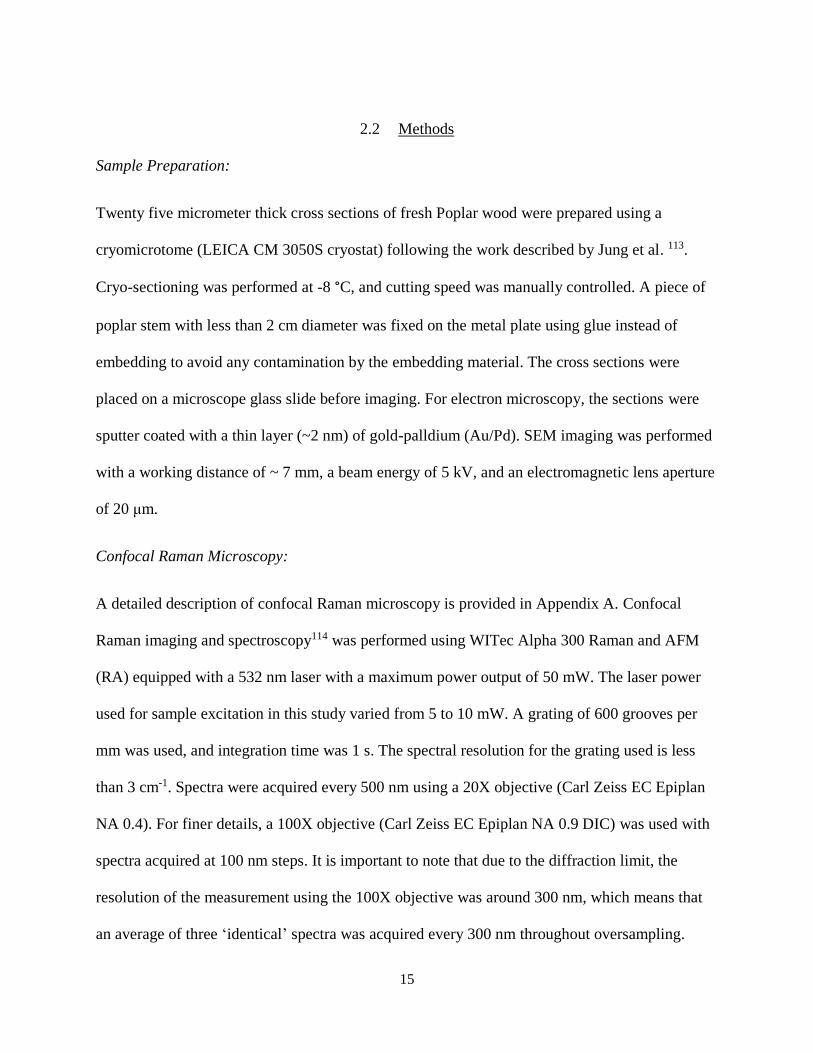
2.2 Methods....................................................................................................................................... 15

2.3 Characterization of the Cell Walls of Normal Wood .................................................................. 19

2.3.1 Chemical Characterization .................................................................................................. 19

2.4 Characterization of the Cell Walls of Tension and Opposite Wood ........................................... 27

2.4.1 Chemical Characterization .................................................................................................. 27

2.4.2 Nanoscale Properties of Tension Wood .............................................................................. 41

2.5 Summary ..................................................................................................................................... 46

3 EFFECTS OF CHEMICAL STRESS IN PLANTS – THE EXAMPLE OF PESTICIDES IN

CITRUS ...................................................................................................................................................... 48

3.1 Background ................................................................................................................................. 48

3.2 Methods....................................................................................................................................... 57

3.2.1 Analytical methods ............................................................................................................. 57

3.2.2 Plant treatment and preparation methods ............................................................................ 59

3.3 Characterization of ZinkicideTM and MS3T ................................................................................ 62

3.3.1 Characterization of ZinkicideTM .......................................................................................... 62

3.3.2 Characterization of MS3T and its Components .................................................................. 76

3.4 The Uptake and Translocation of ZinkicideTM and MS3T in Citrus Seedlings .......................... 83

3.4.1 ZinkicideTM Root Uptake .................................................................................................... 83

3.4.2 MS3T and TSOL Foliar Uptake .......................................................................................... 88

ix

3.5 Summary ..................................................................................................................................... 96

4 UTILIZING EXTERNAL STRESSES IN PLANTS FOR BIOMASS VALORIZATION – THE

EXAMPLES OF BIOMASS FILMS AND GROWTH PROMOTERS ..................................................... 98

4.1 Background ................................................................................................................................. 98

4.2 Example 1: Biomass Films Produced from Lignocellulosic Biomass ...................................... 101

4.2.1 Methods ............................................................................................................................. 101

4.2.2 Characterization of Biomass Films ................................................................................... 104

4.3 Example 2: Improving Yields of Tomato Plants Using Quantum Dots Coated with Growth

Promoters .............................................................................................................................................. 110

4.3.1 Methods ............................................................................................................................. 111

4.3.2 Results ............................................................................................................................... 112

4.4 Summary ................................................................................................................................... 116

5 CONCLUSION ................................................................................................................................. 117

5.1 Overall Summary ...................................................................................................................... 117

5.2 Future Directions ...................................................................................................................... 120

APPENDIX A: BACKGROUND FOR RAMAN SPECTROSCOPY AND IMAGING ........................ 122

APPENDIX B: BACKGROUND FOR FOURIER TRANSFORM INFRARED SPECTROSCOPY .... 126

APPENDIX C: BACKGROUND FOR ATOMIC FORCE MICROSCOPY ........................................... 130

APPENDIX D: COPYRIGHT PERMISSION FOR FIGURE 2.16 ......................................................... 134

APPENDIX E: COPYRIGHT PERMISSIONS FOR FIGURE 3.1 ......................................................... 136

APPENDIX F: COPYRIGHT PERMISSION FOR FIGURE 4.1 ............................................................ 138

LIST OF REFERENCES .......................................................................................................................... 140

x

LIST OF FIGURES

Figure 1.1. The food-water-energy nexus illustrating the interdependence of the components ................... 1

Figure 1.2. Characterization methods at the corresponding length scales probed. The recent access of

advanced atomic force microscopy (AFM), scanning electron microscopy (SEM), and transmission

electron microscopy (TEM) enables the study of several key areas such as the nanoscale structure and

composition of the plant cell walls, the interactions of the main components, and the uptake of

nanoparticle treatments in plants. Nanoscale infrared spectroscopy (nanoIR) and energy dispersive x-ray

spectroscopy (EDS) enable chemical characterization with high resolution. ............................................... 7

Figure 2.1. Schematic representing the arrangement in a section of reaction wood, with tension wood area

represented in red (left). SEM images capture a transition between tension and opposite wood. The red

line indicates the transition in cell wall structure between tension wood and opposite wood. Zoom on the

tension wood cells (right) showing the G layer in the walls. ...................................................................... 11

Figure 2.2: Setup used for Atomic Force Acoustic Microscopy (AFAM). A sinusoidal waveform controls

the actuation of the piezo element placed underneath the sample. The cantilever signal S(t) is analyzed by

lockin amplifier detection to isolate the amplitude and phase of the component at the reference frequency

(actuation frequency). Amplitude and phase are recorded at each point of a predefined map to form the

AFAM image. ............................................................................................................................................. 18

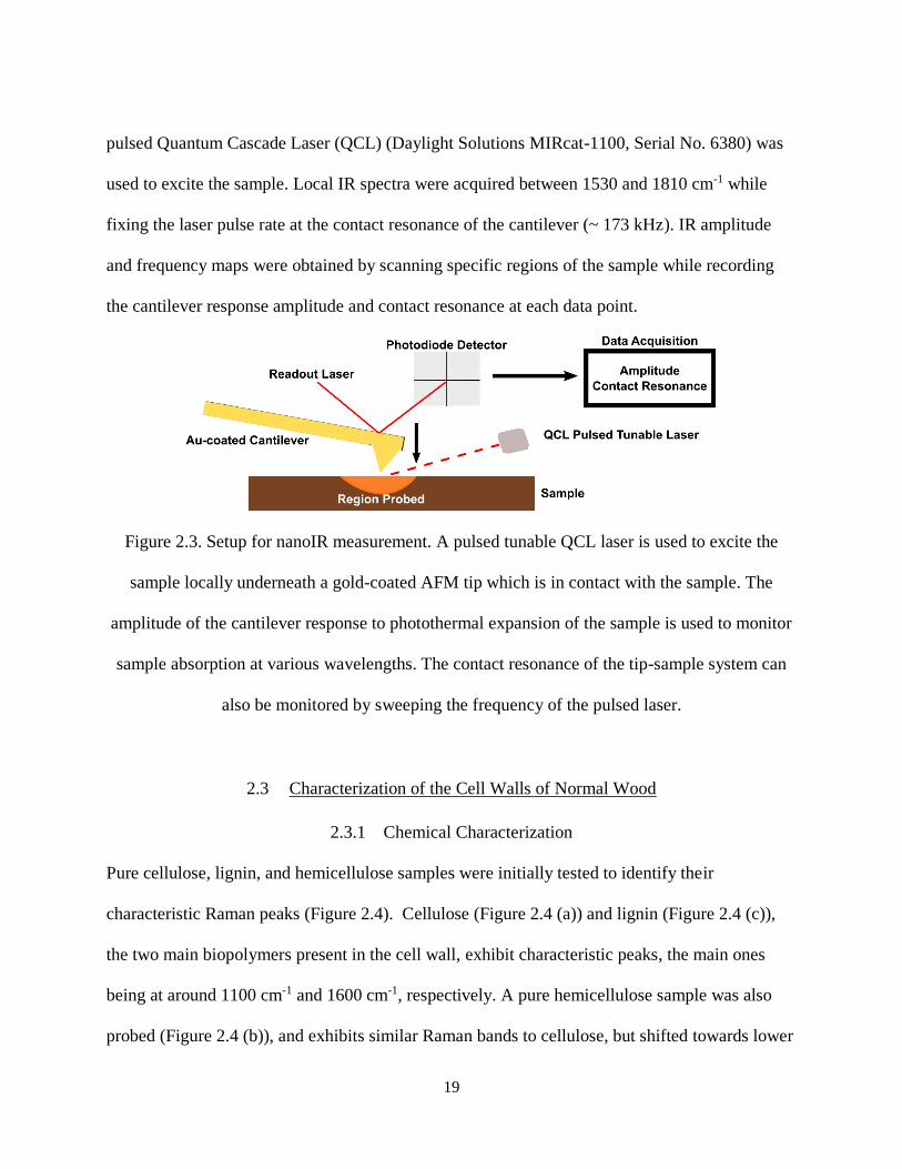
Figure 2.3. Setup for nanoIR measurement. A pulsed tunable QCL laser is used to excite the sample

locally underneath a gold-coated AFM tip which is in contact with the sample. The amplitude of the

cantilever response to photothermal expansion of the sample is used to monitor sample absorption at

various wavelengths. The contact resonance of the tip-sample system can also be monitored by sweeping

the frequency of the pulsed laser................................................................................................................. 19

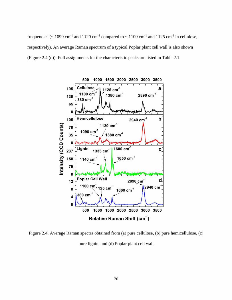
Figure 2.4. Average Raman spectra obtained from (a) pure cellulose, (b) pure hemicellulose, (c) pure

lignin, and (d) Poplar plant cell wall ........................................................................................................... 20

Figure 2.5: Raman intensity maps for cellulose (a) and lignin (b) obtained in the outer regions of a normal

wood cross section. The map for cellulose was constructed using the intensity of the peak at 1100 cm-1

corresponding to C-O-C stretching, and the map for lignin was constructed using the intensity of the peak

at 1600 cm-1 corresponding to aryl ring stretching. Distributions of peak position for the peak at 1100 cm-1

(c) and 1600 cm-1 (d). Distributions of peak width for the peaks at 1100 cm-1 (e) and 1600 cm-1 (f). ....... 23

Figure 2.6: Higher resolution confocal Raman mapping of a normal wood plant cell wall. (a) Optical

image of selected cells in the epidermis of the normal wood cross section. (b, c) Maps representative of

cellulose (b) and lignin (c) constructed by calculating the intensity of their respective Raman peak at 1100

cm-1 and 1600 cm-1. (d) Average spectra of the regions identified by k-means clustering (three clusters).

Map (inset) illustrating the overlay of the 3 clusters corresponding to the lumen (red), secondary (S) layer

(green) and middle lamella (blue). .............................................................................................................. 25

Figure 2.7: Principal component analysis of the Raman spectra obtained from the middle lamella and S

layer in normal wood. (a) Average of the 20 selected spectra selected from the middle lamella and the S

layer. (b) Principal component scores representative of the middle lamella (blue) and the S layer (red). (c)

Loadings of the first principal component. ................................................................................................. 26

Figure 2.8. Raman mapping and cellulose and lignin distribution in the outer region of a Poplar cross

section. (a,b) Maps of the peak intensity (I1100) at 1100 cm-1 representative of cellulose in the tension (a)

and opposite (b) side of the section. (c,d) Distribution of peak position (c) and peak width (d) for the

cellulose band in the range 1095-1108 cm-1. (e,f) Maps of the peak intensity (I1600) at 1600 cm-1

xi

representative of lignin in the tension (e) and opposite (f) side of the section. (g,h) Distribution of peak

position (g) and peak width (h) for the lignin band in the range 1600-1608 cm-1. ..................................... 27

Figure 2.9. Higher resolution confocal Raman mapping of a tension wood cell wall. (a) Optical image of

selected cells in the tension wood. (b, c) Maps representative of cellulose (b) and lignin (c) constructed by

calculating the intensity of their respective Raman peak at 1100 cm-1 and 1600 cm-1. (d) Average spectra

of the regions identified by k-means clustering (four clusters). Map (inset) illustrating the overlay of the 4

clusters corresponding to G layer (red), secondary (S1, S2) layer (green, brown) and middle lamella

(blue). .......................................................................................................................................................... 29

Figure 2.10. Principal component analysis (PCA) of the Raman spectra obtained on the G, S and ML

layers of the tension wood. (a) Average Raman spectra, (b) Principal component scores of PC1 and PC2

representing cluster for G (black), S (red), and ML (blue). (c) PC1 loadings with respect to relative

Raman shift. ................................................................................................................................................ 31

Figure 2.11. Comparison of the cellulose Raman bands in S and G cell wall layers in tension wood.

Areas marked in blue in the G layer (a) and S layer (b) represent the positions from which the spectra are

extracted to construct the histograms in (c-f). (c,d) Distribution of the 1100 cm-1 peak position (c) and

width (d). (e, f) Distribution of the 1380 cm-1 peak position (e) and width (f). .......................................... 32

Figure 2.12. Distribution of the intensity ratio between the cellulose peaks at 380 cm-1 and 1100 cm-1

(I380/I1100) in the G layer (red), S layer (blue), and ML (black) of tension wood. Cellulose crystallinity of

the mean intensity ratio is indicated for each layer. .................................................................................... 35

Figure 2.13. Distribution of the ratio of I1600/I1100 calculated for the tension side (red) and opposite side

(black) with all cell wall layers combined, in the xylem outer layer. ......................................................... 36

Figure 2.14. Variations in cellulose and lignin in the S (a,b) and ML (c,d) layers of the cell wall in tension

(red) and opposite (black) wood. Peak position distributions for characteristic cellulose band around 1100

cm-1 (a,c) and lignin around 1600 cm-1 (b,d). .............................................................................................. 37

Figure 2.15. S/G ratio between the tension (red) and opposite (black) sides compared with normal wood

(blue). (a) The distribution of S/G ratio in the xylem inner layer of tension and normal wood sections. (b)

The distribution of S/G ratio in the xylem outer layer of tension and normal wood sections. ................... 39

Figure 2.16: Comparison of cellulose and lignin peaks position and width distributions in the outer (a-d)

and inner regions (e-h). (a,b) Cellulose peak position and width distribution in the tension and opposite

sides in the outer region. (c,d) Lignin peak position and width distributions in the tension and opposite

sides in the outer region. (e,f) Cellulose peak position and width distributions in the tension and opposite

sides in the inner region. (g,h) Lignin peak position and width distributions in the tension and opposite

sides in the inner region. [adapted from Soliman et al.129].......................................................................... 40

Figure 2.17. Cellulose and lignin distribution in cell walls in the pith. (a,b) Maps of the peak intensity

(I1100) at 1100 cm-1 representative of cellulose in the tension (a) and opposite (b) sides of the section. (c,d)

Distribution of peak position (c) and peak width (d) for the cellulose peak in the range 1095-1105 cm-1.

(e,f) Maps of the peak intensity (I1600) at 1600 cm-1 representative of lignin in the tension (e) and opposite

(f) sides of the section. (g,h) Distribution of peak position (g) and peak width (h) for lignin in the range

1596-1608 cm-1. .......................................................................................................................................... 41

Figure 2.18. Nanoscale investigation of mechanical properties with AFM and AFAM. (a) Topography

image of the tension Poplar wood cross section. (b and c) High resolution topography images. (d and e)

Corresponding AFAM phase images obtained for the higher resolution topography maps in (b) and (c),

respectively. ................................................................................................................................................ 42

Figure 2.19. (a) Distribution of the phase value extracted from the S (red) and G (blue) layer in the

AFAM phase map in Figure 2.18 (e). (b) Comparison in phase variation across nanoscale features in the

cell walls of the S layer (red) and G layer (blue) along the lines in Figure 2.18 (e). .................................. 43

xii

Figure 2.20: Nanoscale infrared spectroscopy measurement using nanoIR. (a) Topography image of a cell

wall on the tension side. (b) Image of the amplitude of cantilever response at the contact resonance. The

image is acquired at the region marked by the white square in (a). (c) Image of the contact resonance

frequency acquired at the same region. Both images in (b) and (c) were acquired at wavenumber (v) =

1640 cm-1. (d) nanoIR spectra acquired at points 1 and 2 marked in (b). (e) First derivative of the nanoIR

spectra shown in (d). (f) Contact resonance spectra acquired at points 1 and 2 marked in (c). .................. 44

Figure 3.1. (a) Representation of a psyllid feeding on sugar in the phloem165. (b) Fluorescence image of

psyllid stylet sheath left behind which shows the path the stylet takes to reach the phloem166. Scale bar in

(b) represents 50 μm. .................................................................................................................................. 51

Figure 3.2. Attributes of ZinkicideTM that have been demonstrated to date................................................ 53

Figure 3.3. Representation of the different modes of application of the treatments ................................... 54

Figure 3.4. Single leaf assay in which a leaf is cut from a seedling and placed in a vial filled with the

treatment solution to test the active ingredient’s movement in the vascular system. ................................. 59

Figure 3.5. Setup for the uptake experiment. (a) Whole seedling assay setup. (b) The shoot part of each

seedling is divided into four segments. (c) Sectioning the leaf blade to obtain leaf extract. ...................... 62

Figure 3.6. Raman spectra of (a) ZinkicideTM SG6 and (b) ZinkicideTM TMN 110. Characteristic bands of

hydrogen peroxide (870 cm-1) and nitrate (1050 cm-1) are present in both formulations. The ratio of peak

intensity of hydrogen peroxide to nitrate is significantly lower in ZinkicideTM TMN 110. ....................... 66

Figure 3.7: FTIR spectra obtained from (a) ZinkicideTM SG6 and (b) ZinkicideTM TMN 110. Significant

variations in the IR spectra are observed between both formulations, for example the band at 740 cm-1 in

ZinkicideTM SG6 shifts to 760 cm-1 with a much lower intensity in ZinkicideTM TMN 110. ..................... 67

Figure 3.8. SEM images of (a) ZinkicideTM TMN 110 and (b) ZinkicideTM TMN 113 aggregates. TMN

110 exhibited a round structure, whereas TMN 113 showed plate-like structures. .................................... 68

Figure 3.9. The solutions tested in the aging study for ZinkicideTM SG6. The solutions were tested on a

weekly basis including the original ZinkicideTM SG6 including the excess reagents, a control with all

ingredients except Zinc nitrate, a washed solution left to age in water from the initial time point, and a

washed solution that is obtained at each time point after aging in the reagents. Each solution was shaken

prior to obtaining 10 μL droplets for measurement. ................................................................................... 69

Figure 3.10. Raman spectra of ZinkicideTM SG6 (a), Washed ZinkicideTM SG6 (b), and the control

solution (c) at the initial time point of the aging study. ZinkicideTM SG6 exhibits hydrogen peroxide (870

cm-1) and nitrate (1050 cm-1) peaks, whereas the washed solution exhibits a Zn peroxide peak (840 cm-1).

.................................................................................................................................................................... 71

Figure 3.11. Evolution of hydrogen peroxide and ZinkicideTM SG6 with respect to water over time.

During the first 12 weeks, the ratio of the intensities of peroxide at ~870 cm-1 to water at ~3400 cm-1

decays over time in ZinkicideTM SG6, but stays fairly constant for the control solution. ........................... 72

Figure 3.12. Average Raman spectra obtained at different time points during the aging of the washed

ZinkicideTM SG6 after aging in water (a) and aging in reagents (b). The peak representing ZnO2 is present

after 12 weeks. ............................................................................................................................................ 73

Figure 3.13. Aging of several initial formulations of agricultural grade ZinkicideTM. The ratio of the

intensities of peroxide (~870 cm-1) and nitrate (1050 cm-1) is presented. ................................................... 75

Figure 3.14. FTIR spectra obtained from (a) TSOL, (b) clay, (c) quaternary compound, and (d) MS3T.

TSOL exhibits a strong broad peak at 1340-1380 cm-1 indicative of nitrate, as well as a peak at ~1620 cm-

1 corresponding to N-H vibrations in urea. MS3T exhibits peaks that can be traced back to the individual

components clay, quaternary compound, and TSOL. ................................................................................. 78

xiii

Figure 3.15. FTIR spectra of urea (U), urea and Zn nitrate (U+ZN), urea and hydrogen peroxide (U+P),

and TSOL. The IR spectra for TSOL and urea and Zn nitrate show shifts in the bands corresponding to

C=O and N-C-N vibrations in urea compared to the IR spectrum of urea.................................................. 80

Figure 3.16. Raman spectra of the different solutions of Zn nitrate and urea used in the titration

experiment. As the concentration of Zn nitrate increases, the peak at 1010 cm-1 corresponding to N-C-N

stretching in urea shifts to higher frequencies. ........................................................................................... 81

Figure 3.17. FTIR spectra of Silica nanoparticles, fixed quat particles, and fixed quat gel (left). The peak

attributed to Si-O-Si in the silica nanoparticles (1070 cm-1) shifts to lower frequencies in the fixed quat

samples (right). ........................................................................................................................................... 82

Figure 3.18. Raman spectra of Silica nanoparticles, fixed quat particles, and fixed quat gel. The peak for

Si-O-Si stretching (1090 cm-1) shifts to 1080 cm-1 in the fixed quat samples. ........................................... 83

Figure 3.19. Average Raman spectra obtained from leaf extracts from different segments of the shoot

system of the seedling following 24 h of uptake. Nitrate at 1050 cm-1, one of the components of

ZinkicideTM, is present in all segments suggesting a movement of the treatment. ..................................... 84

Figure 3.20. SEM images of a citrus leaf midrib cross section (a) and stem cross section (b). Xylem (red)

and phloem (blue) regions are marked on both images. EDS spectra obtained from xylem and phloem

regions in the leaves (c) and stem (d) from all segments of the shoot system after 24 h of uptake. The Zinc

peak at ~ 1.01 keV is present in both the xylem and phloem in leaf and stem tissues compared to the

untreated control (black). ............................................................................................................................ 86

Figure 3.21. Average Zinc concentration (in ppm) in leaves (a) and stem (b) measured by XRF. (c)

Representation of Zinc distribution in a citrus seedling after 6, 12, 18, and 24 h of treatment uptake

reconstructed using concentrations measured by XRF. The distributions show that at 12 and 18 h, the

treatment reaches the leaves in the upper segments, before redistributing to lower leaves at 24 h. ........... 88

Figure 3.22 SEM Imaging of MS3T deposited on the leaf surface after spraying. (a) Untreated leaf surface

showing stomatal openings. (b) MS3T aggregates forming on the leaf surface. (c) MS3T aggregates can

penetrate the stomatal opening. ................................................................................................................... 90

Figure 3.23. Average mean normalized FTIR spectra obtained from untreated control leaves, TSOL

treated leaves, and MS3T treated leaves at (a) 12 h, and (b) 24 h time points. The peak at 1410 cm-1 has a

higher intensity in the untreated leaves than in TSOL or MS3T at 12 h and 24 h. ..................................... 91

Figure 3.24. PCA analysis of IR signatures obtained on untreated and treated citrus leaves after 12 h (a,b)

and 24 h (c,d) of treatment with TSOL and MS3T. Scores plots for 12 h (a) and 24 h (c) treatments

showed separation between treated and untreated clusters. PC Loadings for 12 h (b) and 24 h (d) are also

shown. ......................................................................................................................................................... 93

Figure 3.25. Average Zinc concentration in citrus stems and leaves measured using XRF for (a) TSOL

treated seedlings and (b) MS3T treated seedlings....................................................................................... 94

Figure 3.26. SEM images of treated and untreated leaf midrib cross sections. (a) Treated leaf midrib cross

section. (b) Higher resolution SEM image of the treated leaf midrib cross section (marked by square in

(a)), highlighting regions where EDS measurements were taken (marked by squares). (c) Untreated leaf

midrib cross section. (d) Higher resolution image of the untreated leaf midrib cross section (marked by

square in (c)), crosses mark regions where EDS measurements were acquired. (e) Average EDS spectra

obtained from treated (red) and untreated (black) leaves to determine the presence of Zn (1.01 keV). ..... 95

Figure 4.1. Different routes of obtaining more value from agricultural production in a sustainable manner.

.................................................................................................................................................................. 100

Figure 4.2. Schematic representing a typical force time curve acquired during a PFM scan. Stiffness,

adhesion, and maximum force are indicated. ............................................................................................ 103

xiv

Figure 4.3. Schematic of the setup of LCR. An AC current runs through a special probe which

experiences an oscillating Lorentz force in the presence of an externally applied constant magnetic field.

.................................................................................................................................................................. 104

Figure 4.4. AFM topography images of films prepared using methanol (a,d), DMAc/water (b,e), and

water (c,f) as coagulants. Figure adapted from Wang et al.232. ................................................................. 105

Figure 4.5. (a) Distribution of stiffness values obtained from the PFM measurements. (b) Representative

PFM force curves for water (black), methanol (red) and DMAC/water (blue) films with the adhesion

indicated in the red square. ....................................................................................................................... 106

Figure 4.6. Topography and LCR frequency shift maps of methanol films (a,d), DMAc/water films (b,e),

and water films (c,f). ................................................................................................................................. 107

Figure 4.7. Average Contact Resonance Frequency measured with LCR for the methanol, water and

DMAc/water films. ................................................................................................................................... 108

Figure 4.8. IR spectra obtained at 0% and 50% RH from (a) water film, (b) methanol film, and (c)

DMAc/water film. Blue curves indicate the measurements performed at ambient conditions with 50% RH

while red curves correspond to the measurements performed at low (close to 0%) RH. ......................... 110

Figure 4.9. (a) Optical image. (b) Raman spectra obtained from the stem cross section, bare Nano-Zn, and

SG coated Nano-Zn. (c) Raman map of the intensity of the band at 1040 cm-1 acquired from the region

marked by the white square in (a). (d) SEM image of a stem cross section of the tomato plant treated with

SG coated Nano-Zn. .................................................................................................................................. 113

Figure 4.10. Comparison of the Nano-Zn-Urea, Nano-Zn-NAC, and Nano-Zn-SG treated plants with the

control untreated plants. (a) Relative water content. (b) Membrane stability index. (c) Root length, and (d)

Shoot length. Figure adapted from the study performed by Dr. Smruti Das [unpublished]241. ................ 115

Figure A.1. Basic schematic representing Raman Spectroscopy. Inelastically scattered light is passed

through a diffraction grating prior to reaching the spectrometer to analyze the shift in wavelength relative

to the excitation laser. ............................................................................................................................... 124

Figure B.1. Basic setup for FTIR245 .......................................................................................................... 128

Figure B.2. ATR-FTIR concept. The sample is placed on top of the crystal. An infrared beam is passed

through the crystal and undergoes total internal reflection with the surface in contact with the sample.

Evanescent waves from the beam are absorbed by the sample at the absorption wavelengths before the

beam reaches the detector. ........................................................................................................................ 129

Figure C.1. Basic mechanism for detection of the cantilever deflection in AFM ..................................... 131

xv

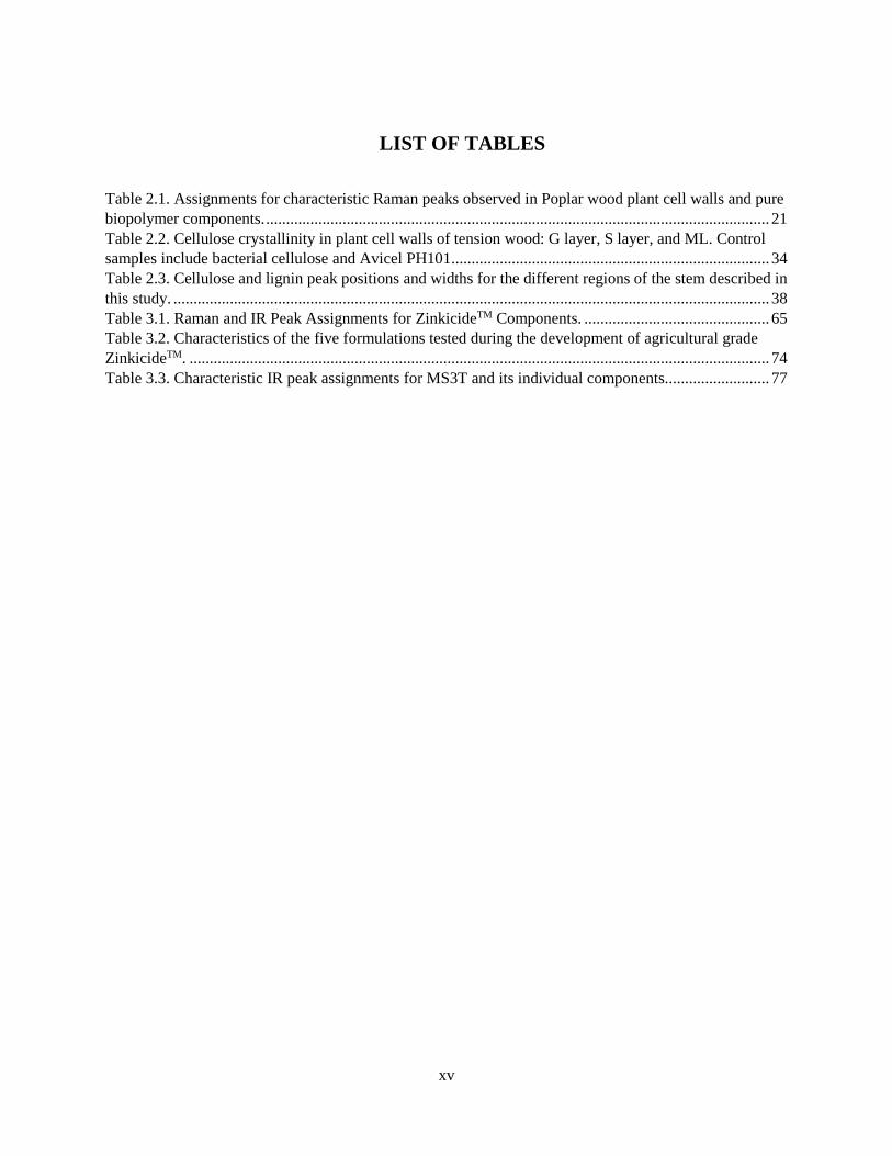
LIST OF TABLES

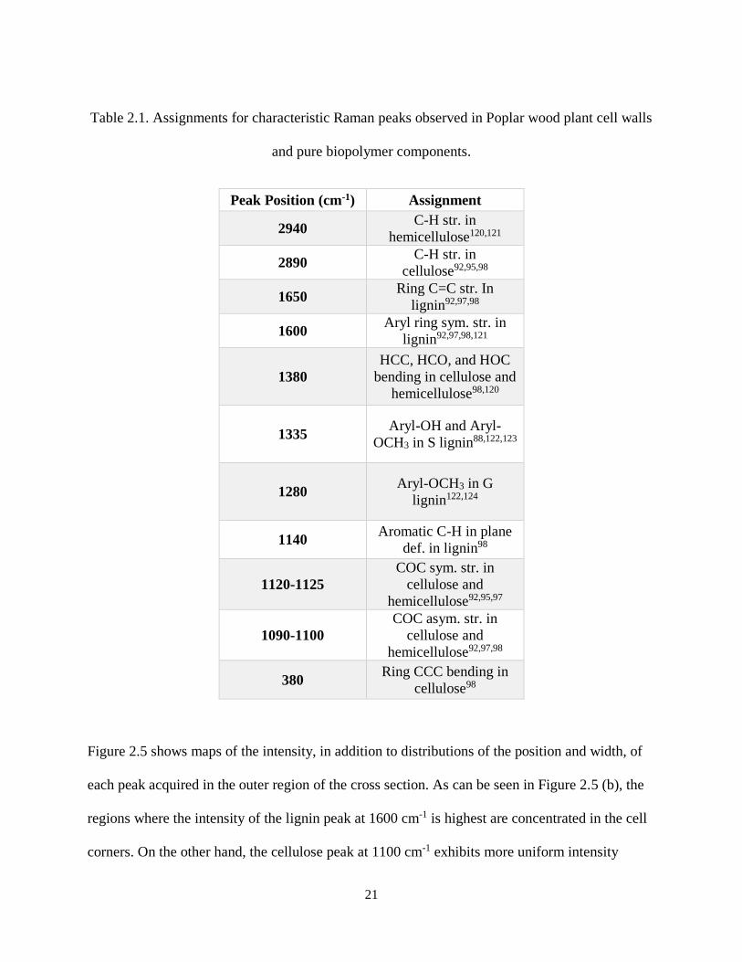
Table 2.1. Assignments for characteristic Raman peaks observed in Poplar wood plant cell walls and pure

biopolymer components. ............................................................................................................................. 21

Table 2.2. Cellulose crystallinity in plant cell walls of tension wood: G layer, S layer, and ML. Control

samples include bacterial cellulose and Avicel PH101 ............................................................................... 34

Table 2.3. Cellulose and lignin peak positions and widths for the different regions of the stem described in

this study. .................................................................................................................................................... 38

Table 3.1. Raman and IR Peak Assignments for ZinkicideTM Components. .............................................. 65

Table 3.2. Characteristics of the five formulations tested during the development of agricultural grade

ZinkicideTM. ................................................................................................................................................ 74

Table 3.3. Characteristic IR peak assignments for MS3T and its individual components.......................... 77

1

1 INTRODUCTION

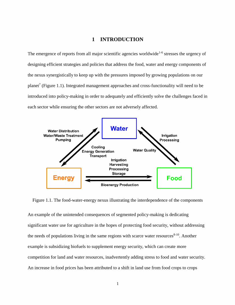
The emergence of reports from all major scientific agencies worldwide1-6 stresses the urgency of

designing efficient strategies and policies that address the food, water and energy components of

the nexus synergistically to keep up with the pressures imposed by growing populations on our

planet7 (Figure 1.1). Integrated management approaches and cross-functionality will need to be

introduced into policy-making in order to adequately and efficiently solve the challenges faced in

each sector while ensuring the other sectors are not adversely affected.

Figure 1.1. The food-water-energy nexus illustrating the interdependence of the components

An example of the unintended consequences of segmented policy-making is dedicating

significant water use for agriculture in the hopes of protecting food security, without addressing

the needs of populations living in the same regions with scarce water resources8-10. Another

example is subsidizing biofuels to supplement energy security, which can create more

competition for land and water resources, inadvertently adding stress to food and water security.

An increase in food prices has been attributed to a shift in land use from food crops to crops

2

dedicated to biofuel production11. As a result, nexus thinking is focused on addressing system

efficiency rather than enhancing productivity in each sector alone12. Moreover, a nexus

perspective would improve the understanding of intricate connections between the three sectors.

Three main pressures for food, water, and energy have been identified: world population

growth, growth of the middle class in developing nations, and climate change12,13. The increasing

world population and demands for resources to sustain or improve quality of life for the

expanding middle class worldwide, pose significant threats to the accessibility to finite resources

in food, energy, and water3,5-7. Climate change adds to the strain on the nexus by lowering the

quality of arable land and threatening clean water resources6. In addition to more efficient

technologies, it is also imperative to utilize the available resources more efficiently than before.

Interdisciplinary scientific research has a crucial role to play in creating innovative solutions to

meet the needs formulated in the scope of this nexus14. Recent advances in nanotechnology, for

instance, may hold a key to ensuring the availability of food to the growing world population15-

18. Nanotechnology also holds promise in the energy19,20 and water21,22 sectors. For instance,

multi-walled carbon nanotubes were previously shown to have 3-4 times the capacity to absorb

contaminant metallic ions in water compared to traditional sorbents used in water purification23.

In terms of energy security, nanotechnology proves useful in a wide range of applications.

Nanostructured composites, for example, are being considered as anode materials to improve

capacity and recharging rate in lithium ion batteries24,25. In food applications, nanotechnology is

promising improvements not just in enhancing agricultural production, but in packaging and

food safety as well. The use of carbon nanotubes for pathogen detection in food packaging has

been studied previously26.

3

The work presented in this dissertation more directly pertains to the energy and food security

sectors. The motivation is to boost our fundamental understanding of plant responses to external

mechanical and chemical stresses using cutting edge characterization with high spatial resolution

and sensitivity, to eventually reach rational design of plant properties and processing for new

solutions applicable to food, energy, and water.

1.1 Studying the Structure and Composition of Plant Cell Walls for more Efficient Bioenergy

Production

In any given country, energy security could be defined as the reliable continuous supply of

energy at an affordable price27,28. Energy security may also refer to energy production and

consumption in a sustainable manner with minimal effects on the environment28. It is estimated

that fossil fuels accounted for 85.5% of total world energy consumption in 201629. Given the

limited supply and the accelerating rate of depletion of the supply, this statistic suggests how

fragile the world’s energy security is for the foreseeable future1. In addition, fossil fuels release a

significant amount of greenhouse gases exacerbating the effects of climate change30. Based on

the definitions above, continued reliance on fossil fuels as the world’s primary source of energy

goes directly against the interest of safeguarding energy security and sustainability.

There are several approaches to overcome the issue of limited energy supply27. First, more

efficient energy consumption can be achieved through measures such as manufacturing cars that

have better fuel economy31, installing building insulation to reduce heat loss32,33, and replacing

incandescent light bulbs with fluorescent lamps or light-emitting diodes34. However, this does

not solve the underlying issue of depleting resources to alarmingly low levels. Therefore,

alternative energy sources that are renewable and clean should be seriously considered. A

4

number of alternative sources are being studied35,36 including: solar power37,38, wind energy39,

tidal energy40, biofuels41-43, geothermal energy44 and hydroelectric power45. Each of these has its

advantages and limitations with regards to how they influence the other sectors of the food-

energy-water nexus. For example, dedicating more land and water use for the production of

biofuels can affect food production as well as clean water supplies. However, biofuels offer a

renewable source of carbon, and if the right practices are implemented, can significantly help

offset the coming rise in demand for energy with minimal effect on the other sectors43. A number

of approaches to minimize the impact of bioenergy production on food and water supply include:

using land that is not dedicated for food production, implementing double land use in which

biofuel crops are grown in between seasons of growing food crops46, and using crop residues and

residues from forestry operations instead of discarding them as waste47,48.

Currently, most of the biofuels produced in the US are obtained from cornstarch49,50. This

threatens crop yields available for consumption and food prices. As a result, the US Energy

Independence and Security Act of 2007 specified that at least 16 of the 36 billion gallon target of

biofuel production by 2022, should come from non-starch sources such as cellulosic biomass41,51.

Cellulosic biomass sources such as switchgrass would also require less irrigation than starch

sources, thereby further reducing potential stresses on water security35.

There is, however, a major obstacle in using cellulosic biomass; namely cellulose extraction due

to the evolved resistance mechanisms to cell wall deconstruction, also known as

recalcitrance52,53. The plant cell walls consist of cellulose fibrils in a matrix of lignin and

hemicellulose54. This complex system is notoriously difficult to break down52,53,55,56. As a result,

the process of cellulose extraction is energy intensive, involving pretreatments and producing

5

significant waste. Therefore, studying in finer details the intricate structure and composition of

the cell wall, which was not previously possible due to the lack of functional analytical tools for

nanoscale characterization, could provide potential solutions to design more efficient processes

to extract cellulose. Moreover, genetic modifications of plant systems informed from this new

understanding for higher cellulose content compared to lignin would also be highly valuable.

1.2 Studying the Uptake and Effects of Chemical Treatments in Plants for Better Plant Disease

Control

The term “food security” refers to the continued access to food and nutrition in terms of

affordability and safety5,12,57,58. Any disruption in food supply at a sufficient scale is considered a

significant threat to any nation’s security. Nowadays, the food supply of the world is under

constant threat due to factors such as climate change, which is predicted to cause an average 8%

decline in food production in Africa and South Asia by the 2050s59,60, and plant diseases which

threaten eradicating important crops such as citrus, potatoes, and tomatoes.

Plant diseases pose the most significant threat in the short term61,62. At least 10% of global food

production is lost to plant diseases, at a time when hundreds of millions of people have

inadequate access to food62. In general, plant pathogens are difficult to control due to numerous

factors including variation in time of infection and geographical spreading, as well as the large

number of dangerous species capable of infecting all of the major crops. It is therefore

imperative to find innovative measures to curb the negative effects plant diseases have on the

food security of the globe. Additionally, these solutions must not affect the other two

components of the nexus adversely. For instance, the increased use of pesticides threatens to

contaminate water resources and levy larger energy costs in terms of storage and frequent

6

application using fuel-operated machinery. Therefore, solutions that could more efficiently

alleviate the effects of plant diseases are sorely needed. One such approach is using nanoparticles

and novel treatments designed from materials which have good antimicrobial properties thus

killing the bacteria rapidly and which can also act as growth promoters to improve crop yields.

1.3 Considering the Importance of Tailoring Characterization Methods and Protocols to the

Problem

To tackle the aforementioned challenges, it is imperative to develop approaches capable of

capturing the variability of natural systems while accessing the interaction-level information at

the subcellular level. Characterization, especially at the nanoscale, constitutes a pillar of the

materials science and engineering field. As more breakthroughs are achieved in nanotechnology

and design of materials, it becomes more necessary to have the ability to probe materials

properties adequately at the nanoscale. This is true for the wide areas of research in which the

potential of nanotechnology is being realized.

In the previous sections, the relation between the work that is presented in this dissertation and

the food and energy components of the food-energy-water nexus was brought to light. At this

point, it is important to highlight the crucial role played by using the appropriate characterization

methods (Figure 1.2) in furthering our knowledge of plant structures and properties at the

nanoscale, as well as in studying the novel treatments designed to protect food crops from plant

diseases and enhance crop yields in view of rising global demands. In terms of plant structure

and properties, it is vital to utilize characterization tools covering multiple scales from the

nanoscale level to study cellulose microfibrils with diameters ranging from a few nanometers to

tens of nanometers, to several micrometers to probe plant cell walls and their layers for instance.

7

Tracking the uptake of treatments in the vascular tissue of plants will also require the ability to

access the phloem, which is normally on the order of several tens of micrometers.

Figure 1.2. Characterization methods at the corresponding length scales probed. The recent

access of advanced atomic force microscopy (AFM), scanning electron microscopy (SEM), and

transmission electron microscopy (TEM) enables the study of several key areas such as the

nanoscale structure and composition of the plant cell walls, the interactions of the main

components, and the uptake of nanoparticle treatments in plants. Nanoscale infrared

spectroscopy (nanoIR) and energy dispersive x-ray spectroscopy (EDS) enable chemical

characterization with high resolution.

8

The mechanisms behind the plant response to mechanical and chemical stresses still need to be

studied in order to make informed decisions on how to utilize these phenomena to our advantage

in securing the world’s natural resources. Within the scope of this work, the phrase “mechanical

stress” is considered in its more general meaning since the effects of different stress components

usually considered in materials science (such as torsion or shear) have not been studied

extensively in plant cells. Nanoscale characterization tools such as advanced modes of atomic

force microscopy are still not employed to their full potential to extract the wealth of knowledge

contained in complex systems like the plant cell walls. Moreover, these same tools could also be

used to study the uptake and effects of promising nanoparticle treatments inside plants and better

appreciate the mode of action of these treatments and how they can eliminate dangerous plant

pathogens.

1.4 Outline of the Present Work

In some plant systems, exposure to mechanical stresses induces a change in composition of the

plant cell walls63-66. In chapter 2, we illustrate this by presenting the example of Poplar tension

wood which forms an extra cellulose-rich layer in the cell wall dubbed the gelatinous (G) layer.

The structure and composition of Poplar tension wood are studied using a number of

characterization techniques including confocal Raman microscopy and advanced atomic force

microscopy (AFM) based methods. Subtle changes in the Raman signature obtained from tension

wood, as compared to opposite and normal wood, are identified using statistical analysis

methods. Potential chemical and mechanical properties variations within the individual cell wall

layers are also explored with advanced AFM techniques.

9

Chapter 3 focuses on the effects of chemical stresses in plants. In particular, we study novel

nanoparticle-based treatments to combat plant diseases. The experimental work performed to

answer key scientific questions about the uptake and effects of treatments designed for use in

citrus plants to combat citrus greening disease, a plant bacterial infection which is currently

decimating citrus crops in Florida and other regions worldwide, is discussed. A protocol

combining multiscale characterization techniques is successfully developed which can

potentially aid growers in designing future strategies for applying these treatments in the field

efficiently to move towards precision agriculture.

Chapter 4 deals with two examples illustrating how the external stresses plants experience can be

utilized to develop added value products in agriculture. In the first example, the properties of

biomass films are studied, as well as the effects of varying processing parameters on them. Apart

from energy production, the financial efficiency of biorefineries may be improved by realizing

the added-value potential of the waste produced from processing biomass into biofuels.

Obtaining new organic materials from biomass as opposed to petroleum would constitute a step

in the direction of sustainability67. In the second example, efficient delivery of growth promoters

using nanoparticles to enhance the yield and physiological traits of tomato plants is explored.

The ability of the plants to uptake the growth promoters is also studied. The example underlines

the potential of nanoparticle-based efficient delivery of growth promoters in minimizing the

negative impact of overuse of fertilizers and pesticides on the environment.

Chapter 5 concludes with a discussion of the implications of the results described in chapters 2,

3, and 4 and relates them to the broader perspective of the energy-water-food nexus. Future

directions and recommendations in each topic are also considered.

10

2 EFFECTS OF MECHANICAL STRESS IN PLANTS – THE EXAMPLE

OF GRAVTY IN POPLAR WOOD

2.1 Background

Mechanical stress can affect the growth and development of all plant species65,66,68-70. Plants can

experience mechanical stress from natural (wind, gravity)71,72, or artificial (touch from foreign

objects)73,74 sources. Changes in the plants structure and composition at the cellular and

subcellular levels, such as altering the cellulose orientation inside the cell walls69 have been

observed. These variations manifest themselves at the macroscale in the form of variations in

root density65, stem size75, the number of leaves76, the surface area of leaves65,76,77, the

concentration of chlorophyll65, and even resistance to disease78 and drought79. These phenomena

occur as a result of plant response at the cellular and subcellular levels, but have not been fully

resolved with conventional characterization tools. The ability to study these changes at the

nanoscale using advanced characterization techniques would significantly aid in understanding

how these stresses at the macroscale can induce alterations in the arrangement of the building

blocks of plant cell walls, as well as changes in composition.

Here we consider reaction wood as an illustration of the potential effect mechanical stresses such

as gravity (gravitropism) can have on wood tissues. In reaction wood, tension and compression

wood are formed as a manifestation of a plant’s natural mechanism to prevent cracking or

breaking. Tension wood forms in hardwoods, whereas compression wood forms in softwoods. In

hardwoods, tension wood forms on the side that is experiencing tensile stress as the branch is

bending. As shown in the Scanning Electron Microscope (SEM) image (Figure 2.1), the

transition from opposite to tension wood along a stem cross section appears to be abrupt. It is

11

now understood that cellulose content in tension wood is high compared to normal wood80 and is

associated with the formation of an extra layer, called the gelatinous (G) layer, in the cell

walls81,82. It was previously reported that G layers contain more cellulose with higher

crystallinity than the other layers of the cell wall81. Moreover, it has been claimed that the

content of S lignin in tension wood is higher than in normal wood, while the content of G lignin

is lower80,83. However, in terms of crystallinity, quantified values for the crystallinity index of

cellulose in tension wood were obtained when measuring the tissue as a whole, and not the

individual cell wall layers84-86. In most cases, the crystallinity index of cellulose is measured

using X-ray Diffraction (XRD) following extensive treatment, such as grinding into powder or

extraction using solvents and thermal treatments, which might influence results. For the S/G

ratio, chemical characterization techniques which require breaking down the sample, such as gas

chromatography, are often used87. However, certain chemometric methods have been used to

quantify the S/G ration previously based on characterization methods such as nuclear magnetic

resonance (NMR)83 and Raman spectroscopy88.

Figure 2.1. Schematic representing the arrangement in a section of reaction wood, with tension

wood area represented in red (left). SEM images capture a transition between tension and

opposite wood. The red line indicates the transition in cell wall structure between tension wood

and opposite wood. Zoom on the tension wood cells (right) showing the G layer in the walls.

12

The capacity of the plant to naturally select cellulose content in the G layer suggests that there

are important key parameters to understand regarding the formation of plant cells. In turn, the

molecular understanding would unlock engineering processes beneficial to producing biomass

that is suitable for biofuel production or for other applications aiming at valorizing

lignocellulosic biomass 80,89. Currently biomass deconstruction of the lignin-hemicellulose-

cellulose complex matrix for further processing is challenging and mainly driven by trial and

error choices of solvents and pretreatment conditions. In order to extract cellulose from the cell

walls, lignin must first be removed using a combination of chemical and thermal processes90,91,

which are energy intensive80.

In this study, reaction wood represents a useful model system to develop approaches capable of

quantitative probing of nanoscale properties that can be related to larger scale measurements.

The development of metrology tools capable of differentiating cellulose and lignin and their

interactions in plant cell walls, at the mesoscale and nanoscale, is of prime interest in this work.

Such model system is relevant according to the surge of isolated studies using nanoscale

metrology tools to explore the complex properties of plant cell walls. Despite the production of

data depicting the localized variations in plant cell walls92-94, a staggering lack of understanding

of the molecular interactions between the wall’s biopolymers constitutes a critical barrier to

realizing the full potential of biomass in energy and material design applications. Isolated and

qualitative analyses of nanoscale images are insufficient to impact material design related to

plant-derived materials. Multiscale and quantitative considerations must be considered to

connect observations made with imaging and spectroscopy to the results obtained with more

conventional characterization for plant science.

13

Confocal Raman microscopy has been used to analyze various components of plant cell wall

layers in their natural state92-98, including the ratio of cellulose to lignin content or the orientation

of cellulose fibers in the different layers of the cell wall96. Agarwal et al. showed further data

analysis can reveal traits such as cellulose crystallinity99,100. Others have used Raman

spectroscopy to investigate the polymorphic modifications of cellulose101. These measurements

were conducted on the plant tissue as a whole, however, and not on individual cell walls or cell

wall layers. Due to the natural variations from one cell wall to another, statistical tools such as

Principal Component Analysis (PCA) and k-means clustering have also been considered to

identify significant variations in the properties of the systems94,95. Despite the rich information

contained in Raman spectra, optical diffraction limits the lateral resolution to a few hundred

nanometers. This considerably impedes the exploration of structures and molecular interactions

within the cell wall, which would require resolving nanoscale features. To overcome this

bottleneck, SEM and AFM-based techniques have been considered to explore nanoscale

structure and properties in plants102-106. For instance, several groups used AFM and force

distance curve analysis to measure the local stiffness of cell walls and discovered variations in

local stiffness between different cell wall layers105,107-109.

As discussed in the preceding paragraphs, advanced characterization methods have already

unveiled a significant amount of information about the structures and properties of plants and

plant cell walls. Nevertheless, there are several questions that still remain, and the full potential

of these characterization methods and data analysis techniques is yet to be realized. In this

chapter, the goal is to expand on the current level of advanced plant characterization by seeking

to extract the maximum possible information from techniques that are already being used and by

14

utilizing novel advanced AFM-based methods to probe potential variations at the nanoscale and

within individual cell wall layers.

We aim to answer the following questions:

1) Can spatially resolved spectroscopy unveil variations in the composition and structure of

the cell walls of plants that experienced mechanical stress?

2) Can we establish new correlations between small scale and layer-scale properties?

3) What are the limitations of existing characterization tools?

As previously mentioned, here we use reaction wood as a model system to demonstrate the rich

information that can be obtained with confocal Raman microscopy and nanoscale imaging

techniques and discuss the connections that require more in-depth studies. We analyze the cell

wall morphology and composition of the outer rings, inner rings, and pith regions on both sides

(tension and opposite) of a stem cross section of Poplar wood. The results are compared to those

obtained in normal (unstressed) wood from the same origin. More specifically, we use statistical

methods to track changes in peak width and position for cellulose and lignin characteristic

Raman bands. Lignin S/G ratio and cellulose crystallinity are among the properties calculated

from our datasets. To explore finer variations in the cell wall, we use Atomic Force Acoustic

Microscopy (AFAM), a technique combining acoustic actuation and AFM, to study potential

variations in the local elastic properties of the cell walls110,111. In order to complement the results

of AFAM, nanoscale infrared spectroscopy (nanoIR)112 is used to analyze variations in chemical

signature at the nanoscale within the individual cell wall layers.

15

2.2 Methods

Sample Preparation:

Twenty five micrometer thick cross sections of fresh Poplar wood were prepared using a

cryomicrotome (LEICA CM 3050S cryostat) following the work described by Jung et al. 113.

Cryo-sectioning was performed at -8 °C, and cutting speed was manually controlled. A piece of

poplar stem with less than 2 cm diameter was fixed on the metal plate using glue instead of

embedding to avoid any contamination by the embedding material. The cross sections were

placed on a microscope glass slide before imaging. For electron microscopy, the sections were

sputter coated with a thin layer (~2 nm) of gold-palldium (Au/Pd). SEM imaging was performed

with a working distance of ~ 7 mm, a beam energy of 5 kV, and an electromagnetic lens aperture

of 20 μm.

Confocal Raman Microscopy:

A detailed description of confocal Raman microscopy is provided in Appendix A. Confocal

Raman imaging and spectroscopy114 was performed using WITec Alpha 300 Raman and AFM

(RA) equipped with a 532 nm laser with a maximum power output of 50 mW. The laser power

used for sample excitation in this study varied from 5 to 10 mW. A grating of 600 grooves per

mm was used, and integration time was 1 s. The spectral resolution for the grating used is less

than 3 cm-1. Spectra were acquired every 500 nm using a 20X objective (Carl Zeiss EC Epiplan

NA 0.4). For finer details, a 100X objective (Carl Zeiss EC Epiplan NA 0.9 DIC) was used with

spectra acquired at 100 nm steps. It is important to note that due to the diffraction limit, the

resolution of the measurement using the 100X objective was around 300 nm, which means that

an average of three ‘identical’ spectra was acquired every 300 nm throughout oversampling.

16

Data Analysis:

WITec Project FOUR+ software was used for data analysis including cosmic ray removal

(CRR), baseline correction, noise filtering, peak fitting, and cluster analysis. For CRR, a filter

size of 4 and a dynamic factor of 8 were applied. This pretreatment was followed by baseline

correction using the shape method, with shape size of 100, noise factor of 1 and smoothing using

Savitzky-Golay algorithm with an order of 3. The traits were studied by monitoring the intensity

of respective peaks for cellulose and lignin. In addition, Lorentz fitting was used to determine the

position of the maximum and the full width at half maximum (FWHM) of the peaks. Values

collected were recorded to form maps and histograms. The draw field feature was used to limit

the data analysis to selected regions in a given image.

K-means clustering115,116 with three clusters for normal wood and four clusters for tension wood

was performed on large data sets using WITec Project FOUR+ software. In addition, Principal

Component Analysis117,118 (PCA) was carried out using Unscrambler X software. For PCA, 20

spectra were selected in each cell wall layer identified by the k-means clustering analysis. Prior

to PCA, the spectra were mean normalized using Unscrambler X.

Crystallinity of Cellulose:

The crystallinity Xc of cellulose was determined based on Agarwal’s work 99,100 using the

following equation:

𝑋𝑐 = [(𝐼380

𝐼1100⁄ )−0.0286

0.0065]% (1)

where I380 and I1100 are the respective intensity of the peaks at 380 cm-1 and 1100 cm-1, which

correspond to bending of ring C-C-C groups and asymmetric stretching of the β-(1-4)-glycosidic

17

bond in cellulose, respectively98. This equation was obtained by a calibration method99 which

involved obtaining Raman spectra from different cellulose samples with known crystallinities

and estimating the peak intensity ratio of the aforementioned peaks for each sample. The

equation is then obtained using regression analysis and can be used to estimate cellulose

crystallinity under any conditions; however, several considerations have to be met99,100,119. The

measurements must be conducted at constant humidity, since it has been shown that humidity

variations influence the crystallinity of cellulose. Additionally, the effects of other components

of the plant cell wall should be considered, such as the increased background fluorescence of

lignin. Background removal is, therefore, essential prior to calculation of the peak intensities to

ensure an accurate result.

Atomic Force Microscopy (AFM), Atomic Force Acoustic Microscopy (AFAM), and Nanoscale

Infrared Spectroscopy (nanoIR):

A detailed explanation of AFM is provided in Appendix C. AFM and AFAM were performed

using WITec Alpha 300 RA. A cantilever with spring constant k ~ 2.7 N/m was used (Tip B,

Mikromasch 11-series). For AFAM, the sample was placed on a piezoelectric transducer vibrated

at the cantilever contact resonance (68 kHz) with amplitude of 10 V. The amplitude and phase of

the cantilever were measured at each point on the image by a lock-in amplifier (Stanford

Instrument SRS SR844) using the actuator driving frequency as reference. The setup for AFAM

measurement is shown in Figure 2.2. Time constant was set at 10 ms and sensitivity was

optimized for the signal measured. Amplitude and phase signals were rerouted to the WITec

18

controller (external channel 1 for amplitude, and external channel 2 for phase) for image

formation.

Figure 2.2: Setup used for Atomic Force Acoustic Microscopy (AFAM). A sinusoidal waveform

controls the actuation of the piezo element placed underneath the sample. The cantilever signal

S(t) is analyzed by lockin amplifier detection to isolate the amplitude and phase of the

component at the reference frequency (actuation frequency). Amplitude and phase are recorded

at each point of a predefined map to form the AFAM image.

Nanoscale infrared spectroscopy (nanoIR) measurements (Figure 2.3) were performed using the

nanoIR2 platform (Anasys Instruments). In nanoIR, a pulsed tunable laser is used to excite the

sample locally directly under the AFM tip. As the sample absorbs the IR light, it expands and

contracts based on the frequency of the pulsed laser. The cantilever oscillates with an amplitude

that is directly related to the sample absorption at each excitation wavelength. By recording the

amplitude of the cantilever response at each wavelength, an IR spectrum is easily obtained for

the position probed with the AFM tip. Another measurement involves sweeping the pulsed laser

frequency (f) to detect shifts in the contact resonance which can be correlated to changes in the

nanomechanical properties. For this measurement, a gold-coated cantilever (Anasys Instruments

Model PR-EX-nIR2-10, k ~ 0.07-0.4 N/m) was mounted to scan the sample in contact mode. A

19

pulsed Quantum Cascade Laser (QCL) (Daylight Solutions MIRcat-1100, Serial No. 6380) was

used to excite the sample. Local IR spectra were acquired between 1530 and 1810 cm-1 while

fixing the laser pulse rate at the contact resonance of the cantilever (~ 173 kHz). IR amplitude

and frequency maps were obtained by scanning specific regions of the sample while recording

the cantilever response amplitude and contact resonance at each data point.

Figure 2.3. Setup for nanoIR measurement. A pulsed tunable QCL laser is used to excite the

sample locally underneath a gold-coated AFM tip which is in contact with the sample. The

amplitude of the cantilever response to photothermal expansion of the sample is used to monitor

sample absorption at various wavelengths. The contact resonance of the tip-sample system can

also be monitored by sweeping the frequency of the pulsed laser.

2.3 Characterization of the Cell Walls of Normal Wood

2.3.1 Chemical Characterization

Pure cellulose, lignin, and hemicellulose samples were initially tested to identify their

characteristic Raman peaks (Figure 2.4). Cellulose (Figure 2.4 (a)) and lignin (Figure 2.4 (c)),

the two main biopolymers present in the cell wall, exhibit characteristic peaks, the main ones

being at around 1100 cm-1 and 1600 cm-1, respectively. A pure hemicellulose sample was also

probed (Figure 2.4 (b)), and exhibits similar Raman bands to cellulose, but shifted towards lower

20

frequencies (~ 1090 cm-1 and 1120 cm-1 compared to ~ 1100 cm-1 and 1125 cm-1 in cellulose,

respectively). An average Raman spectrum of a typical Poplar plant cell wall is also shown

(Figure 2.4 (d)). Full assignments for the characteristic peaks are listed in Table 2.1.

Figure 2.4. Average Raman spectra obtained from (a) pure cellulose, (b) pure hemicellulose, (c)

pure lignin, and (d) Poplar plant cell wall

21

Table 2.1. Assignments for characteristic Raman peaks observed in Poplar wood plant cell walls

and pure biopolymer components.

Peak Position (cm-1) Assignment

2940 C-H str. in

hemicellulose120,121

2890 C-H str. in

cellulose92,95,98

1650 Ring C=C str. In

lignin92,97,98

1600 Aryl ring sym. str. in

lignin92,97,98,121

1380

HCC, HCO, and HOC

bending in cellulose and

hemicellulose98,120

1335 Aryl-OH and Aryl-

OCH3 in S lignin88,122,123

1280 Aryl-OCH3 in G

lignin122,124

1140 Aromatic C-H in plane

def. in lignin98

1120-1125

COC sym. str. in

cellulose and

hemicellulose92,95,97

1090-1100

COC asym. str. in

cellulose and

hemicellulose92,97,98

380 Ring CCC bending in

cellulose98

Figure 2.5 shows maps of the intensity, in addition to distributions of the position and width, of

each peak acquired in the outer region of the cross section. As can be seen in Figure 2.5 (b), the

regions where the intensity of the lignin peak at 1600 cm-1 is highest are concentrated in the cell

corners. On the other hand, the cellulose peak at 1100 cm-1 exhibits more uniform intensity

22

indicating the presence of cellulose in the walls. Figures 2.5 (c) and (d) show the distributions of

the peak positions for the peaks around 1100 cm-1 and 1600 cm-1, respectively. The peak

corresponding to cellulose has an average position of around 1094 cm-1, whereas the peak

corresponding to lignin has an average position of around 1598 cm-1. Similar analysis was

performed in the inner region and the pith of the same normal wood cross section and shows that

the peak positions of cellulose and lignin varied compared to the values obtained in the outer

region, with cellulose having an average peak position at ~ 1097 cm-1 and lignin at ~ 1602 cm-1

in the inner region, whereas in the pith cellulose has an average peak position at ~1099 cm-1 and

lignin at ~ 1605 cm-1. This shows that the different rings present within a single cross section can

have some variation in their properties.

23

Figure 2.5: Raman intensity maps for cellulose (a) and lignin (b) obtained in the outer regions of

a normal wood cross section. The map for cellulose was constructed using the intensity of the

peak at 1100 cm-1 corresponding to C-O-C stretching, and the map for lignin was constructed

using the intensity of the peak at 1600 cm-1 corresponding to aryl ring stretching. Distributions of

peak position for the peak at 1100 cm-1 (c) and 1600 cm-1 (d). Distributions of peak width for the

peaks at 1100 cm-1 (e) and 1600 cm-1 (f).

24

Higher resolution Raman mapping was also acquired (with a 100X objective) on normal wood

cell walls to study variations between the individual cell wall layers (Figure 2.6). Chemical maps

of cellulose (Figure 2.6 (b)) and lignin (Figure 2.6 (c)) distribution in the cell wall were

constructed using the intensities of the bands at 1100 cm-1 and 1600 cm-1, respectively. The

chemical maps show that lignin is more concentrated in the middle lamella and the cell corners.

Cellulose is more uniformly distributed across the cell walls. K-means clustering (Figure 2.6 (d))

is capable of differentiating between the layers, with three clusters separating the middle lamella,

the S layer, and the lumen. The average spectra calculated from each cluster show that the

middle lamella has higher intensity for peaks representative of lignin at around 1335 cm-1 and

1600 cm-1 compared to the S layer. On the other hand, the peak representative of cellulose

(around 1100 cm-1) has about the same intensity in the S layer and the middle lamella, which

suggests significant presence of cellulose in the middle lamella.

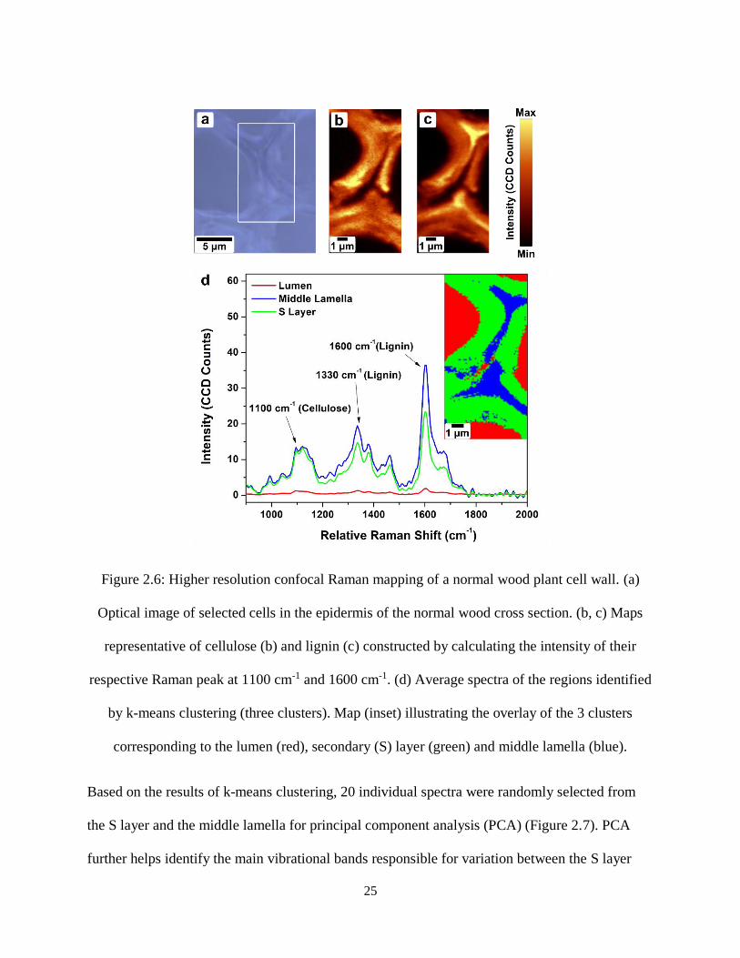
25

Figure 2.6: Higher resolution confocal Raman mapping of a normal wood plant cell wall. (a)

Optical image of selected cells in the epidermis of the normal wood cross section. (b, c) Maps

representative of cellulose (b) and lignin (c) constructed by calculating the intensity of their

respective Raman peak at 1100 cm-1 and 1600 cm-1. (d) Average spectra of the regions identified

by k-means clustering (three clusters). Map (inset) illustrating the overlay of the 3 clusters

corresponding to the lumen (red), secondary (S) layer (green) and middle lamella (blue).

Based on the results of k-means clustering, 20 individual spectra were randomly selected from

the S layer and the middle lamella for principal component analysis (PCA) (Figure 2.7). PCA

further helps identify the main vibrational bands responsible for variation between the S layer

26

and the middle lamella. The scores plot (Figure 2.7 (b)) for the first and second principal

components (PC1 and PC2) show that there is separation between the spectra obtained from the

middle lamella and those obtained from the S layer along the axis representing PC1, which is

responsible for 75% of variation in the data. Separation along PC2, which is responsible for 4%

of variation, is not observed. The loadings of PC1 (Figure 2.7 (c)) show that the major sources of

variation occur at 1335 cm-1 and 1600 cm-1, corresponding to aryl ring vibrations in lignin, and at

2890 cm-1 corresponding to C-H stretching in cellulose. It is interesting to note that the results

showed less variation in the cellulose band around 1100 cm-1 based on the small PC 1 loading

observed for this band, which agrees with the k-means clustering result.

Figure 2.7: Principal component analysis of the Raman spectra obtained from the middle lamella

and S layer in normal wood. (a) Average of the 20 selected spectra selected from the middle

lamella and the S layer. (b) Principal component scores representative of the middle lamella

(blue) and the S layer (red). (c) Loadings of the first principal component.

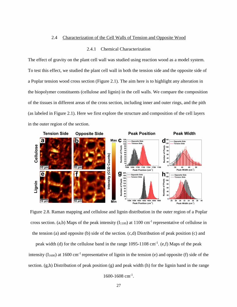
27

2.4 Characterization of the Cell Walls of Tension and Opposite Wood

2.4.1 Chemical Characterization

The effect of gravity on the plant cell wall was studied using reaction wood as a model system.

To test this effect, we studied the plant cell wall in both the tension side and the opposite side of

a Poplar tension wood cross section (Figure 2.1). The aim here is to highlight any alteration in

the biopolymer constituents (cellulose and lignin) in the cell walls. We compare the composition

of the tissues in different areas of the cross section, including inner and outer rings, and the pith

(as labeled in Figure 2.1). Here we first explore the structure and composition of the cell layers

in the outer region of the section.

Figure 2.8. Raman mapping and cellulose and lignin distribution in the outer region of a Poplar

cross section. (a,b) Maps of the peak intensity (I1100) at 1100 cm-1 representative of cellulose in

the tension (a) and opposite (b) side of the section. (c,d) Distribution of peak position (c) and

peak width (d) for the cellulose band in the range 1095-1108 cm-1. (e,f) Maps of the peak

intensity (I1600) at 1600 cm-1 representative of lignin in the tension (e) and opposite (f) side of the

section. (g,h) Distribution of peak position (g) and peak width (h) for the lignin band in the range

1600-1608 cm-1.

28

In Figure 2.8, the distributions of cellulose and lignin in the cell walls of the outer region of the

tension and opposite sides of the cross sections were calculated based on the Raman spectra

obtained in both sides of the stem cross section. All measurements were carried out with the

same configuration and settings. The maps presented in Figure 2.8 (a, b) were constructed by

calculating the intensity at the peak maximum (~1100 cm-1) corresponding to the vibration of β-

(1-4)-glycosidic bond in cellulose. A shift in the position of this peak is found from 1102 cm-1 in

the tension side to 1099 cm-1 in the opposite side, and peak width from 42 cm-1 in the tension

side to 40 cm-1 in the opposite side. The shift is above the spectral resolution of the instrument.

This highlights variations in the cell wall cellulose structure between the tension and opposite

sides. Similar shifts are observed in the lignin peak position (1602 cm-1 in the opposite side to

1605 cm-1 in the tension side) and width (from 33 cm-1 in the opposite side to 31 cm-1 in the

tension side) of the band characteristic of lignin around 1600 cm-1 (C=C in the aromatic ring) 92.

These changes could indicate that the lignin structure or environment at the molecular level is

different between the tension and opposite sides. Additionally, the maps constructed by

calculating the maximum peak intensity of the Raman band at 1600 cm-1 (Figure 2.8 (e,f))

indicate that lignin is more concentrated in the middle lamella and cell corners.

29

Figure 2.9. Higher resolution confocal Raman mapping of a tension wood cell wall. (a) Optical

image of selected cells in the tension wood. (b, c) Maps representative of cellulose (b) and lignin

(c) constructed by calculating the intensity of their respective Raman peak at 1100 cm-1 and 1600

cm-1. (d) Average spectra of the regions identified by k-means clustering (four clusters). Map

(inset) illustrating the overlay of the 4 clusters corresponding to G layer (red), secondary (S1, S2)

layer (green, brown) and middle lamella (blue).

To better understand the shifts in cellulose and lignin characteristic peak position and width

observed in Figure 2.8, we acquired a higher resolution map of the plant cell wall composition on

the tension side using a 100x objective (Figure 2.9). The distribution of cellulose in Figure 2.9

30

(b) and lignin in Figure 2.9 (c) is in good agreement with the maps in Figure 2.8 (e,f) in that

lignin concentration is the highest in the lamella and cell corner while cellulose is more

prominent in the S and G layers.

The average spectra calculated from each cluster reveal variations in cellulose content and

cellulose to lignin ratio between the layers. The results confirm that the G layer (red in Figure 2.9

(d)) is very rich in cellulose as seen from the large peak in the 1050-1150 range cm-1, which can

also be assigned to hemicellulose120,125, and rather low lignin signal around 1600 cm-1. On the

other hand, the middle lamella presents a large peak around 1600 cm-1, indicative of higher

lignin content. The bands at 1335 cm-1 and 1380 cm-1 are indicative of bending vibrations

resulting from cellulose98 but the peak at 1335 cm-1 may also be attributed to aryl-OH or aryl-

OCH3 vibrations in lignin88,98,122. The cellulose band intensity at ~ 1100 cm-1 in the lamella is the

lowest of all layers. The secondary wall reveals two different signatures with the region closest

to the lamella showing strong peaks for lignin and cellulose, in addition to a strong peak at 1335

cm-1. The region closest to the G layer shows a much lower peak at 1335 cm-1 and 1600 cm-1,

which suggests a larger contribution from lignin to the 1335 cm-1 band.

The properties of tension wood were further investigated by performing PCA on the spectra

extracted from the Raman image (Figure 2.10). In contrast to k-means clustering, PCA

differentiates three layers: the middle lamella, the S layer, and the G layer. The advantage of k-

means clustering in this study is the ability to overlay the clusters identified with the plant cell

wall image. The average spectra corresponding to each layer are presented in Figure 2.10 (a).

Two predominant PCA components are identified: PC1 accounts for 58% of the variations, while

PC2 accounts for 31%. Figure 2.10 (b) shows that the data is grouped into three main clusters

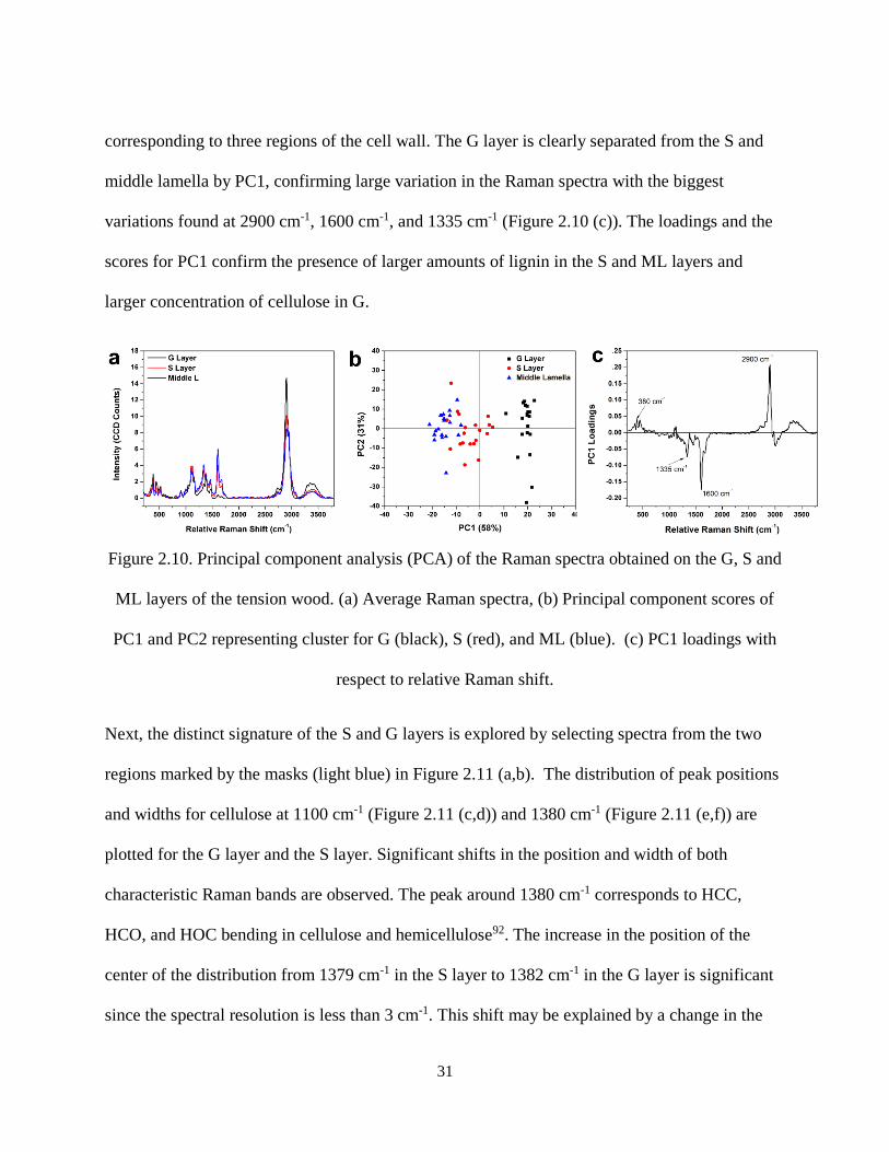
31

corresponding to three regions of the cell wall. The G layer is clearly separated from the S and

middle lamella by PC1, confirming large variation in the Raman spectra with the biggest

variations found at 2900 cm-1, 1600 cm-1, and 1335 cm-1 (Figure 2.10 (c)). The loadings and the

scores for PC1 confirm the presence of larger amounts of lignin in the S and ML layers and

larger concentration of cellulose in G.

Figure 2.10. Principal component analysis (PCA) of the Raman spectra obtained on the G, S and

ML layers of the tension wood. (a) Average Raman spectra, (b) Principal component scores of

PC1 and PC2 representing cluster for G (black), S (red), and ML (blue). (c) PC1 loadings with

respect to relative Raman shift.

Next, the distinct signature of the S and G layers is explored by selecting spectra from the two

regions marked by the masks (light blue) in Figure 2.11 (a,b). The distribution of peak positions

and widths for cellulose at 1100 cm-1 (Figure 2.11 (c,d)) and 1380 cm-1 (Figure 2.11 (e,f)) are

plotted for the G layer and the S layer. Significant shifts in the position and width of both

characteristic Raman bands are observed. The peak around 1380 cm-1 corresponds to HCC,

HCO, and HOC bending in cellulose and hemicellulose92. The increase in the position of the

center of the distribution from 1379 cm-1 in the S layer to 1382 cm-1 in the G layer is significant

since the spectral resolution is less than 3 cm-1. This shift may be explained by a change in the

32

environment (such as residual stresses) surrounding these molecules, or the orientation of the

cellulose microfibrils96. For instance, lignin is present in a greater amount in the S layer than in

the G layer54. The changes observed in the 1100 cm-1 peak width with a much narrower peak in

the G layer than in the S layer, suggest different properties of the cellulose microfibrils in the S

and G layers. Similar variations have previously been attributed to changes in crystallinity99,126.

Additionally, changes in cellulose characteristic peak positions have been attributed to changes

in stress and strain in the microfibrils127,128, as well as orientation97.

Figure 2.11. Comparison of the cellulose Raman bands in S and G cell wall layers in tension

wood. Areas marked in blue in the G layer (a) and S layer (b) represent the positions from which

the spectra are extracted to construct the histograms in (c-f). (c,d) Distribution of the 1100 cm-1

peak position (c) and width (d). (e, f) Distribution of the 1380 cm-1 peak position (e) and width

(f).

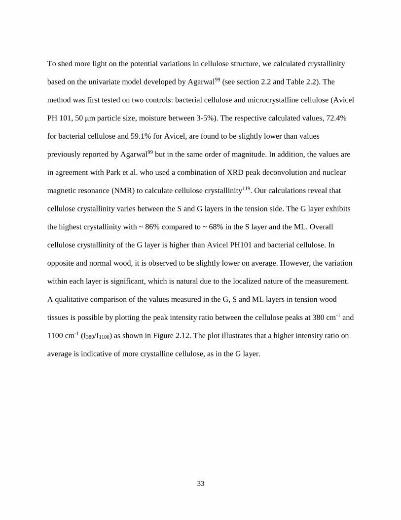
33

To shed more light on the potential variations in cellulose structure, we calculated crystallinity

based on the univariate model developed by Agarwal99 (see section 2.2 and Table 2.2). The

method was first tested on two controls: bacterial cellulose and microcrystalline cellulose (Avicel

PH 101, 50 μm particle size, moisture between 3-5%). The respective calculated values, 72.4%

for bacterial cellulose and 59.1% for Avicel, are found to be slightly lower than values

previously reported by Agarwal99 but in the same order of magnitude. In addition, the values are

in agreement with Park et al. who used a combination of XRD peak deconvolution and nuclear

magnetic resonance (NMR) to calculate cellulose crystallinity119. Our calculations reveal that

cellulose crystallinity varies between the S and G layers in the tension side. The G layer exhibits

the highest crystallinity with ~ 86% compared to ~ 68% in the S layer and the ML. Overall

cellulose crystallinity of the G layer is higher than Avicel PH101 and bacterial cellulose. In

opposite and normal wood, it is observed to be slightly lower on average. However, the variation

within each layer is significant, which is natural due to the localized nature of the measurement.

A qualitative comparison of the values measured in the G, S and ML layers in tension wood

tissues is possible by plotting the peak intensity ratio between the cellulose peaks at 380 cm-1 and

1100 cm-1 (I380/I1100) as shown in Figure 2.12. The plot illustrates that a higher intensity ratio on

average is indicative of more crystalline cellulose, as in the G layer.

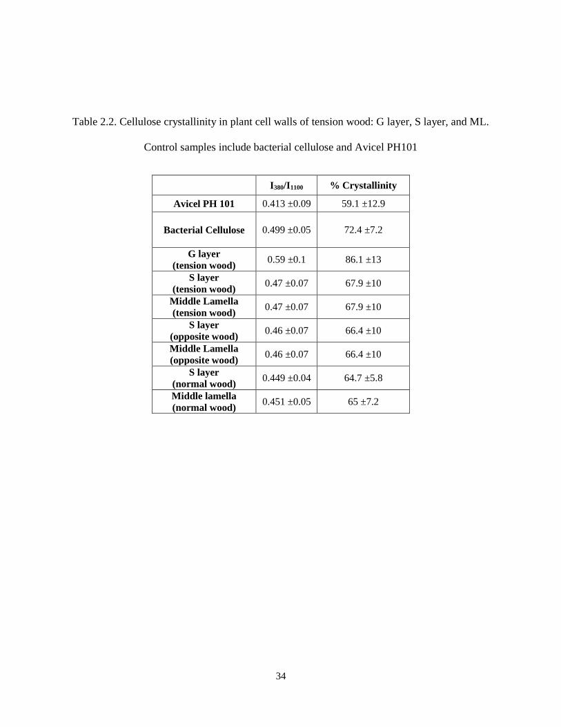
34

Table 2.2. Cellulose crystallinity in plant cell walls of tension wood: G layer, S layer, and ML.

Control samples include bacterial cellulose and Avicel PH101

I380/I1100 % Crystallinity

Avicel PH 101 0.413 ±0.09 59.1 ±12.9

Bacterial Cellulose 0.499 ±0.05 72.4 ±7.2

G layer

(tension wood) 0.59 ±0.1 86.1 ±13

S layer

(tension wood) 0.47 ±0.07 67.9 ±10

Middle Lamella

(tension wood) 0.47 ±0.07 67.9 ±10

S layer

(opposite wood) 0.46 ±0.07 66.4 ±10

Middle Lamella

(opposite wood) 0.46 ±0.07 66.4 ±10

S layer

(normal wood) 0.449 ±0.04 64.7 ±5.8

Middle lamella

(normal wood) 0.451 ±0.05 65 ±7.2

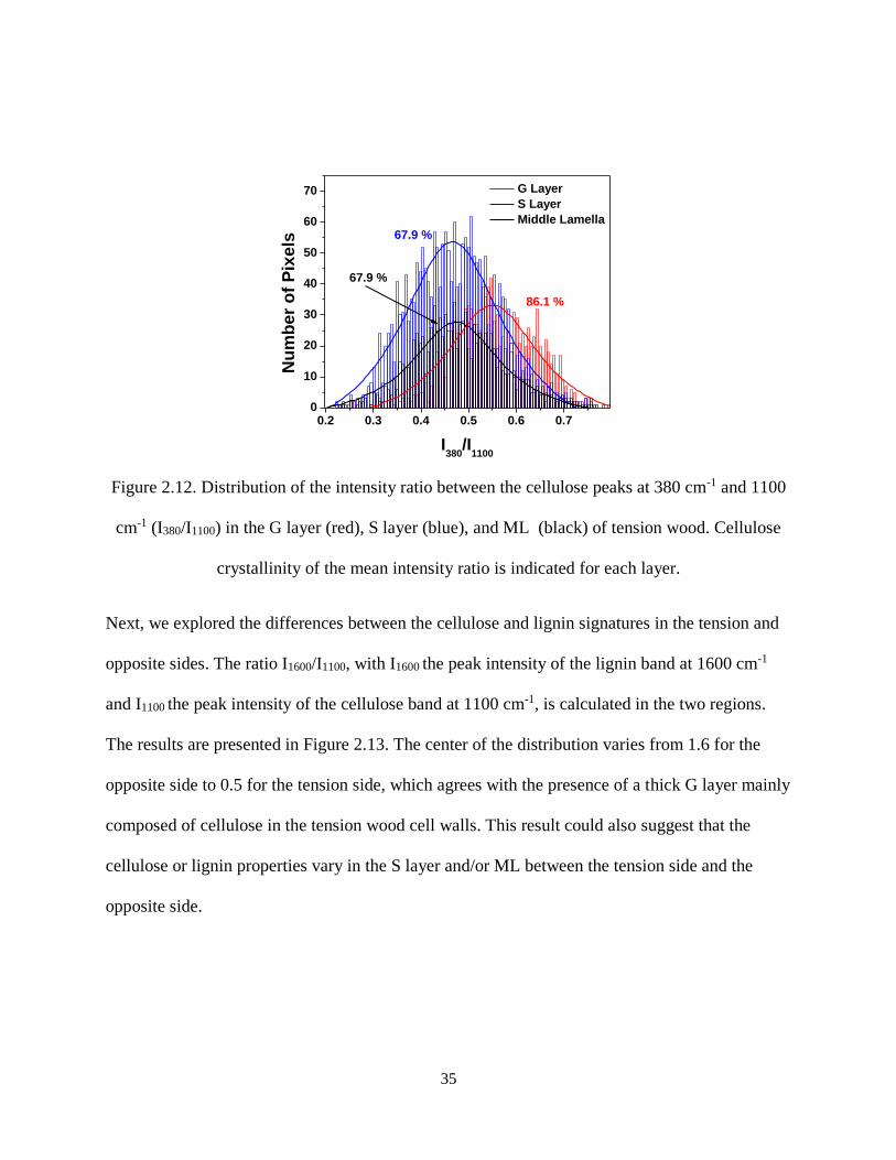
35

Figure 2.12. Distribution of the intensity ratio between the cellulose peaks at 380 cm-1 and 1100

cm-1 (I380/I1100) in the G layer (red), S layer (blue), and ML (black) of tension wood. Cellulose

crystallinity of the mean intensity ratio is indicated for each layer.

Next, we explored the differences between the cellulose and lignin signatures in the tension and

opposite sides. The ratio I1600/I1100, with I1600 the peak intensity of the lignin band at 1600 cm-1

and I1100 the peak intensity of the cellulose band at 1100 cm-1, is calculated in the two regions.

The results are presented in Figure 2.13. The center of the distribution varies from 1.6 for the

opposite side to 0.5 for the tension side, which agrees with the presence of a thick G layer mainly

composed of cellulose in the tension wood cell walls. This result could also suggest that the

cellulose or lignin properties vary in the S layer and/or ML between the tension side and the

opposite side.

0.2 0.3 0.4 0.5 0.6 0.70

10

20

30

40

50

60

70

86.1 %

67.9 %N

um

ber

of

Pix

els

I380

/I1100

G Layer

S Layer

Middle Lamella

67.9 %

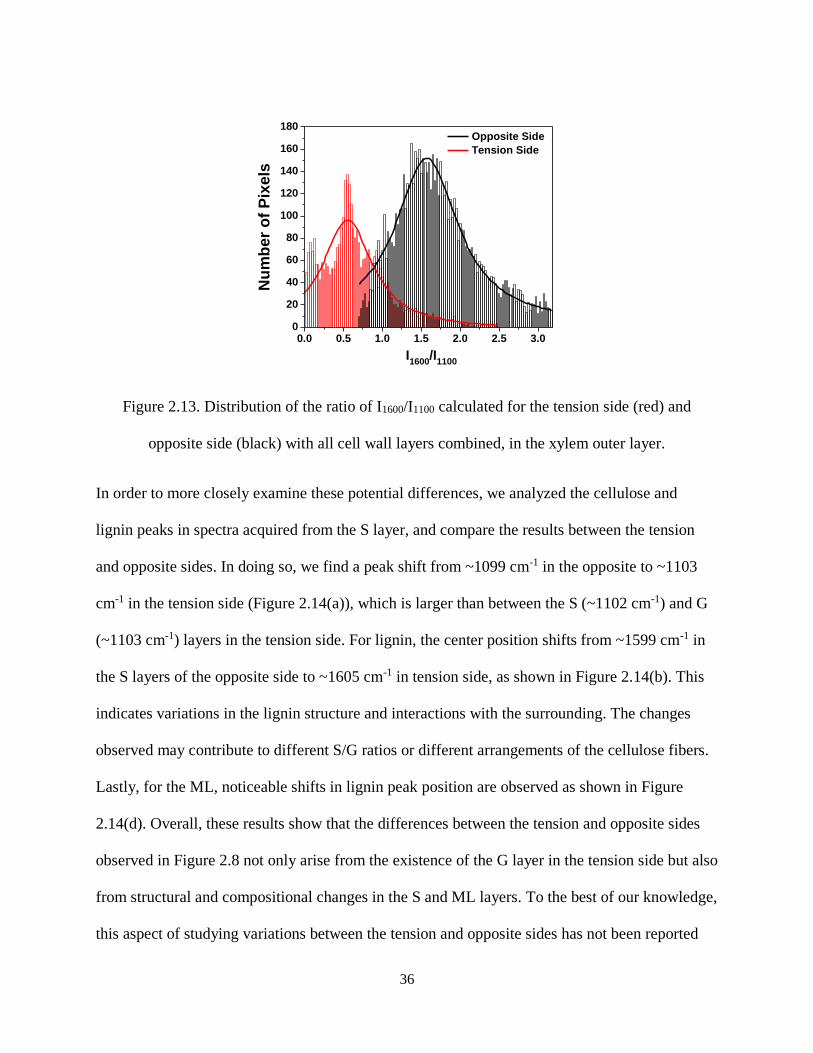
36

Figure 2.13. Distribution of the ratio of I1600/I1100 calculated for the tension side (red) and

opposite side (black) with all cell wall layers combined, in the xylem outer layer.

In order to more closely examine these potential differences, we analyzed the cellulose and

lignin peaks in spectra acquired from the S layer, and compare the results between the tension

and opposite sides. In doing so, we find a peak shift from ~1099 cm-1 in the opposite to ~1103

cm-1 in the tension side (Figure 2.14(a)), which is larger than between the S (~1102 cm-1) and G

(~1103 cm-1) layers in the tension side. For lignin, the center position shifts from ~1599 cm-1 in

the S layers of the opposite side to ~1605 cm-1 in tension side, as shown in Figure 2.14(b). This

indicates variations in the lignin structure and interactions with the surrounding. The changes

observed may contribute to different S/G ratios or different arrangements of the cellulose fibers.

Lastly, for the ML, noticeable shifts in lignin peak position are observed as shown in Figure

2.14(d). Overall, these results show that the differences between the tension and opposite sides

observed in Figure 2.8 not only arise from the existence of the G layer in the tension side but also

from structural and compositional changes in the S and ML layers. To the best of our knowledge,

this aspect of studying variations between the tension and opposite sides has not been reported

0.0 0.5 1.0 1.5 2.0 2.5 3.00

20

40

60

80

100

120

140

160

180

Nu

mb

er

of

Pix

els

Opposite Side

Tension Side

I1600

/I1100

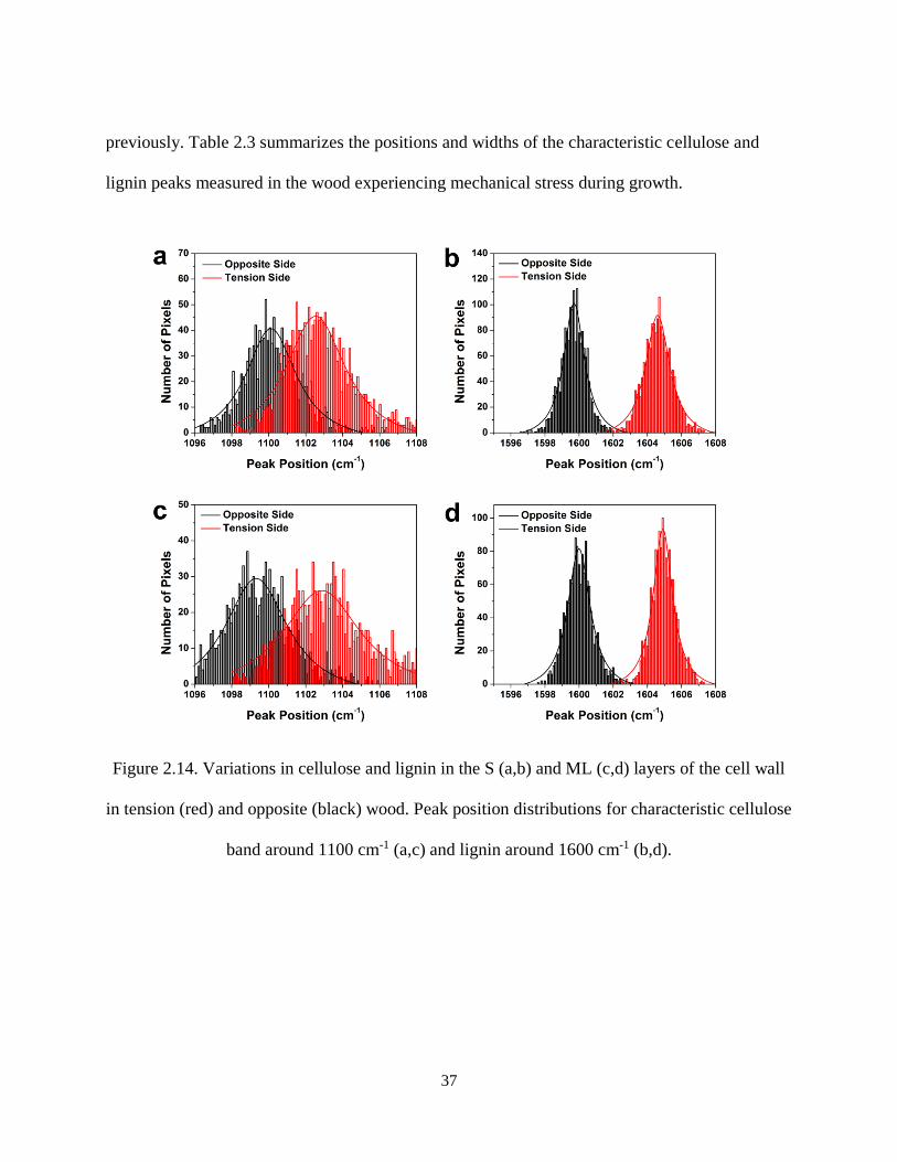
37

previously. Table 2.3 summarizes the positions and widths of the characteristic cellulose and

lignin peaks measured in the wood experiencing mechanical stress during growth.

Figure 2.14. Variations in cellulose and lignin in the S (a,b) and ML (c,d) layers of the cell wall

in tension (red) and opposite (black) wood. Peak position distributions for characteristic cellulose

band around 1100 cm-1 (a,c) and lignin around 1600 cm-1 (b,d).

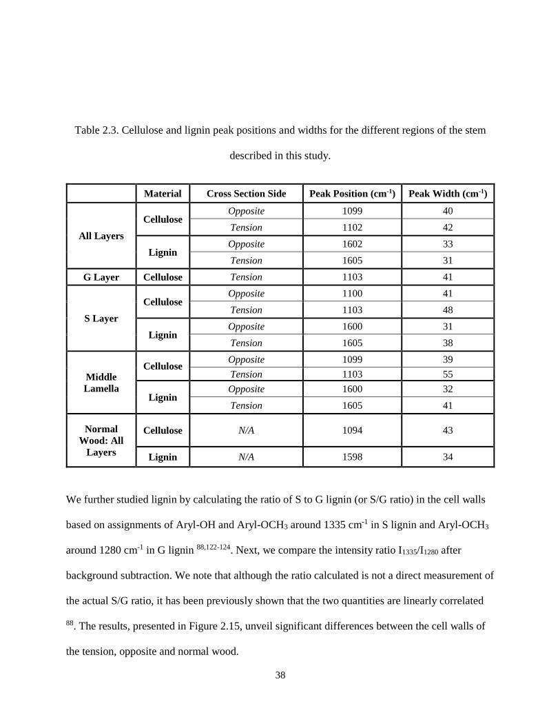
38

Table 2.3. Cellulose and lignin peak positions and widths for the different regions of the stem

described in this study.

Material Cross Section Side Peak Position (cm-1) Peak Width (cm-1)

All Layers

Cellulose Opposite 1099 40

Tension 1102 42

Lignin Opposite 1602 33

Tension 1605 31

G Layer Cellulose Tension 1103 41

S Layer

Cellulose Opposite 1100 41

Tension 1103 48

Lignin Opposite 1600 31

Tension 1605 38

Middle

Lamella

Cellulose Opposite 1099 39

Tension 1103 55

Lignin Opposite 1600 32

Tension 1605 41

Normal

Wood: All

Layers

Cellulose N/A 1094 43

Lignin N/A 1598 34

We further studied lignin by calculating the ratio of S to G lignin (or S/G ratio) in the cell walls

based on assignments of Aryl-OH and Aryl-OCH3 around 1335 cm-1 in S lignin and Aryl-OCH3

around 1280 cm-1 in G lignin 88,122-124. Next, we compare the intensity ratio I1335/I1280 after

background subtraction. We note that although the ratio calculated is not a direct measurement of

the actual S/G ratio, it has been previously shown that the two quantities are linearly correlated

88. The results, presented in Figure 2.15, unveil significant differences between the cell walls of

the tension, opposite and normal wood.

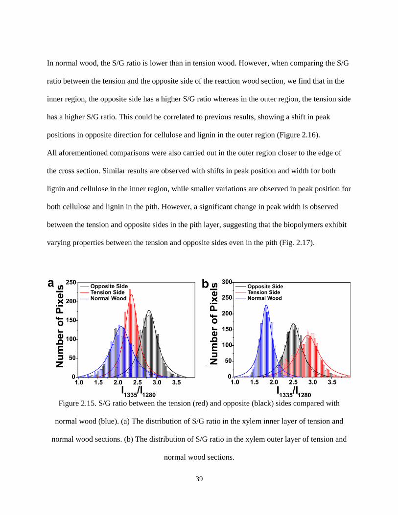
39

In normal wood, the S/G ratio is lower than in tension wood. However, when comparing the S/G

ratio between the tension and the opposite side of the reaction wood section, we find that in the

inner region, the opposite side has a higher S/G ratio whereas in the outer region, the tension side

has a higher S/G ratio. This could be correlated to previous results, showing a shift in peak

positions in opposite direction for cellulose and lignin in the outer region (Figure 2.16).

All aforementioned comparisons were also carried out in the outer region closer to the edge of

the cross section. Similar results are observed with shifts in peak position and width for both

lignin and cellulose in the inner region, while smaller variations are observed in peak position for

both cellulose and lignin in the pith. However, a significant change in peak width is observed

between the tension and opposite sides in the pith layer, suggesting that the biopolymers exhibit

varying properties between the tension and opposite sides even in the pith (Fig. 2.17).

Figure 2.15. S/G ratio between the tension (red) and opposite (black) sides compared with

normal wood (blue). (a) The distribution of S/G ratio in the xylem inner layer of tension and

normal wood sections. (b) The distribution of S/G ratio in the xylem outer layer of tension and

normal wood sections.

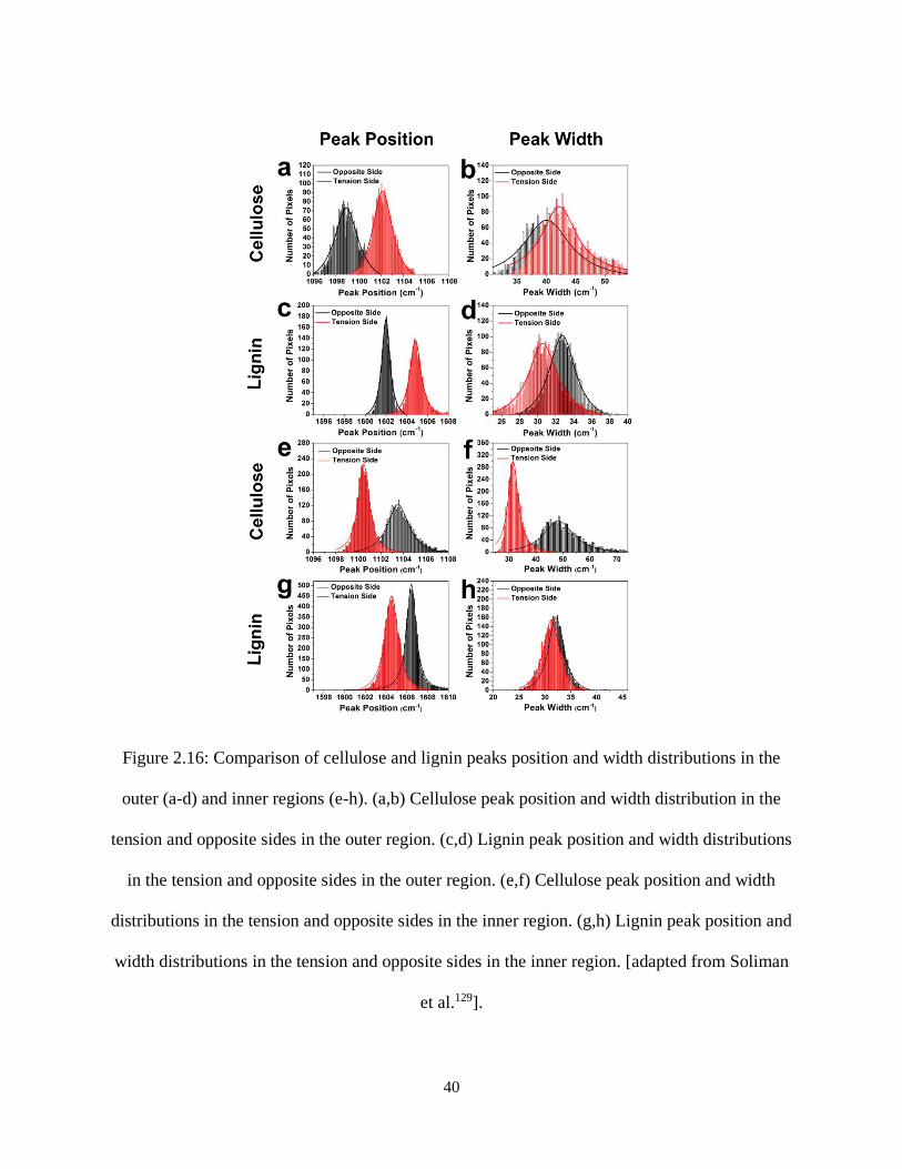
40

Figure 2.16: Comparison of cellulose and lignin peaks position and width distributions in the

outer (a-d) and inner regions (e-h). (a,b) Cellulose peak position and width distribution in the

tension and opposite sides in the outer region. (c,d) Lignin peak position and width distributions

in the tension and opposite sides in the outer region. (e,f) Cellulose peak position and width

distributions in the tension and opposite sides in the inner region. (g,h) Lignin peak position and

width distributions in the tension and opposite sides in the inner region. [adapted from Soliman

et al.129].

41

Figure 2.17. Cellulose and lignin distribution in cell walls in the pith. (a,b) Maps of the peak

intensity (I1100) at 1100 cm-1 representative of cellulose in the tension (a) and opposite (b) sides

of the section. (c,d) Distribution of peak position (c) and peak width (d) for the cellulose peak in

the range 1095-1105 cm-1. (e,f) Maps of the peak intensity (I1600) at 1600 cm-1 representative of

lignin in the tension (e) and opposite (f) sides of the section. (g,h) Distribution of peak position

(g) and peak width (h) for lignin in the range 1596-1608 cm-1.

2.4.2 Nanoscale Properties of Tension Wood

Thus far Raman spectroscopy has revealed chemical and structural changes, such as crystallinity

of cellulose, in the cell walls across the stem; however, a tool that can help visualize these

changes at the nanoscale remains highly desirable. Confocal Raman microscopy suffers from the

optical diffraction limit, restricting its lateral resolution. To overcome this challenge, we consider

42

a platform capable of measuring nanoscale variations in mechanical or chemical properties

observed with functional AFM (AFAM and nanoIR, see section 2.2).

AFAM maps of the local variations in mechanical properties or subsurface features has

previously been reported 130-132. Figure 2.18 (e), representing the AFAM phase signal, highlights

the details unveiled with nanoscale imaging, well beyond the resolution achieved with confocal

Raman spectroscopy or standard AFM (Figure 2.18 (b,c)).

Figure 2.18. Nanoscale investigation of mechanical properties with AFM and AFAM. (a)

Topography image of the tension Poplar wood cross section. (b and c) High resolution

topography images. (d and e) Corresponding AFAM phase images obtained for the higher

resolution topography maps in (b) and (c), respectively.

43

Figure 2.19. (a) Distribution of the phase value extracted from the S (red) and G (blue) layer in

the AFAM phase map in Figure 2.18 (e). (b) Comparison in phase variation across nanoscale

features in the cell walls of the S layer (red) and G layer (blue) along the lines in Figure 2.18 (e).

Interestingly, a comparison of the phase measurements recorded across the S and the G layer

suggests that the acoustic wave propagation is affected by the nature of the material. Figure 2.19

(a) shows the distribution of the phase measured using AFAM in the S and G layers in Figure

2.18 (e). The plot reveals a variation of around 0.4o in the center average of the phase measured,

with both distributions exhibiting roughly the same width. Figure 2.19 (b) shows profiles

extracted from the S and G layers along the section markers, red and blue lines indicated in

Figure 2.18 (e). The curves show a variation in phase on the order of a few degrees within a 200

nm distance in both the S and G layers. This finding suggests that the phase signal in AFAM

measurements is sensitive to local variations in structure and/or properties in each layer of the

cell wall. The phase signal is particularly important in this measurement as it can relate to the

contact stiffness and damping in the tip-sample system133. In general, the phase increases with

increasing contact stiffness, and decreases with increasing damping133. This suggests that AFAM

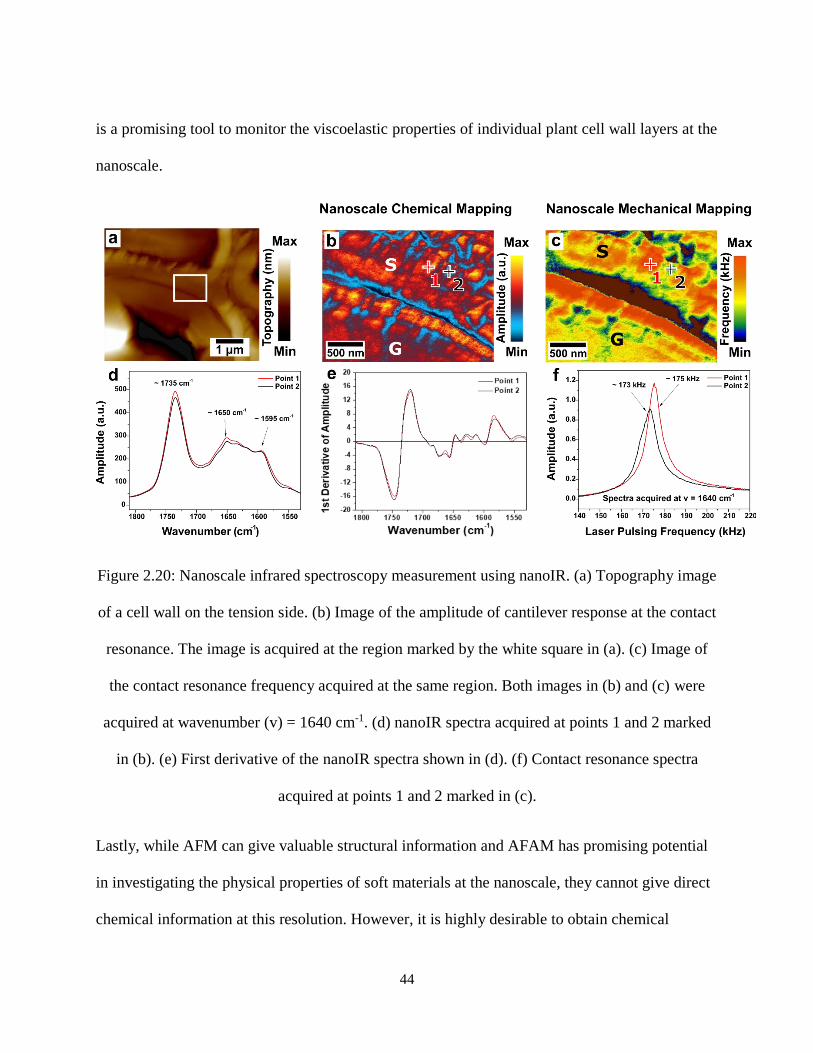
44

is a promising tool to monitor the viscoelastic properties of individual plant cell wall layers at the

nanoscale.

Figure 2.20: Nanoscale infrared spectroscopy measurement using nanoIR. (a) Topography image

of a cell wall on the tension side. (b) Image of the amplitude of cantilever response at the contact

resonance. The image is acquired at the region marked by the white square in (a). (c) Image of

the contact resonance frequency acquired at the same region. Both images in (b) and (c) were

spectra acquired at points 1 and 2 marked anoIR n. (d) 1-avenumber (v) = 1640 cmacquired at w

in (b). (e) First derivative of the nanoIR spectra shown in (d). (f) Contact resonance spectra

acquired at points 1 and 2 marked in (c).

Lastly, while AFM can give valuable structural information and AFAM has promising potential

in investigating the physical properties of soft materials at the nanoscale, they cannot give direct

chemical information at this resolution. However, it is highly desirable to obtain chemical

45

information at the nanoscale. To address this shortcoming, the chemical characterization

capability of infrared spectroscopy with the nanoscale spatial resolution of the AFM has been

developed in the form of nanoIR112. Here, we used nanoIR to investigate the chemical properties

within a S and G layer of the tension side. The maps of the cantilever response amplitude and

contact resonance frequency at a fixed laser wavenumber (1640 cm-1, which corresponds to OH

bending vibrations adsorbed on cellulose) 134,135 are presented in Figure 2.20. Furthermore, IR

single spectra were acquired at locations exhibiting low and high amplitudes indicated by points

1 and 2 in Figure 2.20 (b). The amplitude of the resonance was measured at fixed pulsed laser

frequency of 173 kHz (Figure 2.20 (d)). The variations in the IR map indicate chemical

inhomogeneity within the S layer; however, the IR spectra shown in Figure 2.20 (d) acquired

from points 1 and 2 do not exhibit significant variation in the IR signature. To confirm this, we

obtained first derivatives of the IR spectra (Figure 2.20 (e)) which again do not show variation in

the chemical signature between points 1 and 2. On the other hand, the contact resonance

measured at points 1 and 2 (Figure 2.20 (f)) showed a clear shift from 175 kHz in point 1 to 173

kHz in point 2, which is indicative of a higher local stiffness in the plant cell wall at point 1 than

at point 2 since a higher contact resonance frequency corresponds to greater local stiffness. One

possible explanation for this result is that the nanochemical measurement includes photothermal

expansion of a larger volume underneath the AFM tip, which means that the measurement is

actually detecting an average contribution of highly heterogeneous materials in the volume,

whereas the nanomechanical measurement involves just the local interaction between the tip and

the sample at the point being measured without displacement of the point measured. These

findings suggest that AFAM may be influenced by chemistry and/or stiffness, but the two cannot

46

be readily decorrelated at this point. Nonetheless, this approach paves the way to a deeper

understanding of individual cell wall layers composition and properties in plant tissues.

2.5 Summary

Confocal Raman microscopy and statistical analysis reveal variations in cellulose and lignin

properties and their distributions in the tension, opposite and normal wood. These features could

not be resolved without sub-micrometer microscopy capabilities. Using k-means clustering, the

different layers of the cell wall on the tension side can be identified, and variations in the peak

position and width of two of the characteristic cellulose Raman bands are observed in the

different layers. The S/G ratio for lignin is estimated to be higher in tension wood than in normal

wood which is in agreement with previous studies 80,83. The crystallinity of cellulose within the

cell wall layers, estimated from the Raman spectra, reveals that G layers exhibit the highest

crystallinity while cellulose in the S layer and the ML of tension wood is found to be slightly

more crystalline than in opposite and normal wood.

These results show that we can monitor variations in the composition and structure of the cell

walls of plants that experienced mechanical stress using spatially resolved spectroscopy

techniques. We also show that it is possible to monitor nanoscale mechanical properties using

advanced AFM-based methods such as AFAM and nanoIR. This enables characterization of

properties within the individual cell wall layers. One limitation encountered in using nanoIR is

the fact that the QCL pulsed laser excites a larger volume in the sample, which hinders the

measurement of nanoscale chemical composition, especially in a complex system as the plant

cell wall. The nanomechanical measurement, on the other hand, involves effects that are

47

localized to where the tip is in contact with the sample, and is therefore more sensitive to

nanoscale variations within the cell wall layers.

One challenge that remains is to link the nanoscale variations to the changes observed at the

layer-scale (~ few micrometers). An interesting future study is to use AFAM to monitor

nanoscale mechanical property changes within the S layer in tension wood, and to determine if

there is any correlation between these changes and the shifts in cellulose or lignin Raman peak

position and width observed in Figure 2.14.

In the long term, these studies can significantly aid in materials design applications for bioenergy

and added value products manufacturing from lignocellulosic biomass. The ability to control the

properties of plant cell walls at the nanoscale can enable the design of more favorable structure

and composition to enhance the efficiency of biomass deconstruction. This path holds promise in

terms of sustainability and protecting the food-energy-water nexus.

48

3 EFFECTS OF CHEMICAL STRESS IN PLANTS – THE EXAMPLE OF

PESTICIDES IN CITRUS

3.1 Background

Plants can experience chemical stresses from the multitude of sources of artificial chemicals and

pesticides applied on an industrial scale to crops around the world. The effects of chemicals used

to treat plants, prevent or eradicate plant diseases and promote crop yields is an important topic

of research due to its implications on the environment and safety of consumers. The use of

nanoparticles is especially significant. For instance, carbon-based fullerol nanoparticles have

been shown to increase bitter melon fruit yields by up to 59%136, and the use of ceria

nanoparticles in wheat showed a 12.7% improvement in shoot biomass and a 36.6%

improvement in grain yield137. As indicated in the examples, nanoparticles can induce stresses

which can potentially cause fundamental changes in the plants properties138,139. In this chapter,

we address the issue of chemical stress in plants. We focus on an application relevant to

sustainable agriculture. More specifically, we address the need to combat plant diseases that are

severely reducing citrus crop yields.

To address the basic necessity of providing food for the world’s growing population, the

importance of increasing the efficient use of arable land will continue to grow in coming years.

The goal is to double the production of food worldwide by 20505,13. To achieve this, significant

obstacles shall be overcome, such as eradicating epidemics of plant diseases and pest

infestations, limiting overuse of pesticides with harmful side effects on the environment,

managing soil erosion, and addressing declining biodiversity and desertification due to climate

change and other threats140.

49

Over the years different methods have been used to cope with these challenges such as

improving soil quality141 and efficient water use142, as well as enhancing crop yields with

fertilizers143 and pesticides144. Nutrients have also been used to improve agricultural production

either by soil application to improve soil fertility141,145 or by foliar application to the plant

directly146-149. In fact, nitrogen supply alone is responsible for 30-60% of yield in crops such as

grain, corn, and cotton. Researchers also claim that this figure would be even higher if other

nutrient inputs such as phosphorous or potassium were factored in143.

As beneficial as nutritious fertilizers are for agricultural production, they provide limited support

for plant disease treatments. A number of pathogens continuously threaten crops, putting food

production in jeopardy around the world61. Bacterial infections such as pseudomonas syringae

pathovars and Ralstonia Solanacearum, both of which infect a variety of plant species including

tomatoes150,151, potatoes152, and tobacco153,154, have caused significant economic losses to the

agricultural industry61. Ralstonia Solanacearum has caused losses of ~US$1 billion per year in

potato crops alone. This particular pathogen is challenging due to its adaptability, variation in

strains, and the wide range of plants it can infect, making potatoes unusable for potato-based

products. Ralstonia Solanacearum is a soil-borne pathogen and it infects the plant by entering

through wounds or cracks in the root, then translocating systemically to the shoot system of the

plant where it colonizes the xylem tissue61. Xylem and phloem-restricted pathogens constitute an

important threat to food production155-157, due to the difficulty associated with detecting the

early onset of the disease, as well as the lack of efficient methods to directly target (control or

eradicate) the bacteria inside the plants using existing pesticides. Another systemic disease,

called Citrus Greening and also known as Huanglongbing (HLB)158, constitutes our case study

here. HLB, which infects the phloem of citrus plants, has been decimating citrus crops in Florida,

50

and other regions of the world such as Brazil and Asia159. There are also alarming signs the

disease is spreading to California and Texas. In Califorina, the first detection of HLB occurred in

2013, and until now the disease does not seem to have spread to all citrus groves160. In Texas, the

disease was first detected in 2012161, and is already spreading at an alarming rate. In Florida,

HLB is caused by the bacterial species Candidatus Liberibacter asiaticus (CLas). The bacteria

are transferred to the phloem of the citrus plants through a vector, the Asian Citrus Psyllid

(ACP)162, an insect that feeds on the sugar transported through the phloem by extending a stylet

which can penetrate into the vascular system of the leaves. During the feeding process, ACPs can

inject the bacteria into the phloem, as shown in Figure 3.1. The pathogens can rapidly transfer

from the leaves phloem to the roots163. As the bacterial colonies grow, the transport of important

nutrients and water is hindered, slowly causing lower fruit yield with a sugar to acid content

unsuitable for consumption. Overall, HLB has caused a US$7.8 billion loss in Florida’s citrus

industry alone between 2007 and 2016164.

51

Figure 3.1. (a) Representation of a psyllid feeding on sugar in the phloem165. (b) Fluorescence

image of psyllid stylet sheath left behind which shows the path the stylet takes to reach the

phloem166. Scale bar in (b) represents 50 μm.

A number of methods have been and continue to be considered to combat HLB to varying

degrees of success. Thermal treatment (or thermotherapy) has initially shown some promise167.

Best management practices and quarantining of infected regions have helped in sustaining some

citrus production; however, as is the case with the former methods, none of these solutions

directly target and eliminate the disease inside the plants. Breeding and genetic engineering have

also showed some improvement in the resistance of the plants to the disease but will likely

require several years before the technology becomes fully matured168,169. All these methods are

very costly to the growers.

In the meantime, growers are using a variety of insecticide products to control ACP170, as well as

antibiotics to control HLB171,172. Conventional insecticides targeting ACP have showed some

52

promise162,170. For instance, field trials by researchers at the University of Florida’s Institute of

Food and Agricultural Sciences (UF-IFAS) yielded a guide for growers to apply several

commercial insecticides such as Imidacloprid and Fenpropathrin173. However, it has been

recently shown that ACP already developed resistance to Imidacloprid, Fenpropathrin, as well as

other key insecticides in Florida174. Moreover, these insecticides can control the vector, but do

nothing to the bacteria colonizing the vascular system of the plants170. Antibiotics have been

considered to act systemically by directly targeting the bacteria through direct injection172.

However, it was shown that the antibiotics do not reach the target vascular tissue at a

concentration high enough to kill the bacteria171.

With these considerations in mind, a new nanoparticle-based treatment was designed by Dr.

Swadeshmukul Santra at the University of Central Florida175. The vision for this treatment was to

overcome the limitation of standard pesticides by allowing systemic movement of bactericidal

actives in the plant. To achieve this, the core particles should maintain a diameter below 5 nm to

cross the natural barriers inside the plant, such as the casparian strip which blocks the apoplastic

route of transport176. In addition, to circumvent resistance developing for copper (Cu) in bacterial

colony, the treatment was developed with ZnO, which has also been shown to have antibacterial

properties177-179, but is used less commonly than Cu. Pathogens are still not resistant to Zn. The

ZnO-based nanoparticle treatment was dubbed ZinkicideTM 175. Figure 3.2 shows some of the

favorable attributes of ZinkicideTM. The formulation developed by Santra’s lab175 has already

shown some promise in combatting another plant disease, Citrus Canker180. Three modes of

application have been considered for this treatment to date: foliar, root uptake, and trunk

injection (Figure 3.3).

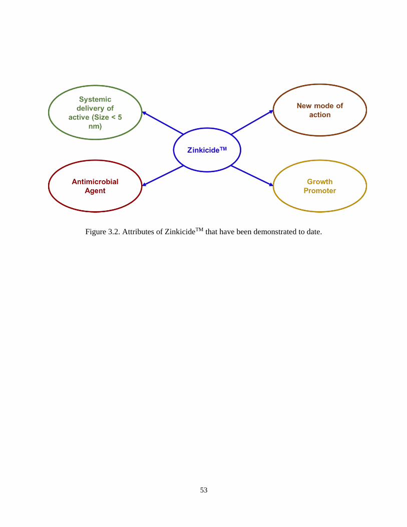
53

Figure 3.2. Attributes of ZinkicideTM that have been demonstrated to date.

54

Figure 3.3. Representation of the different modes of application of the treatments

In addition to its antibacterial activity, Zn is considered as an important element with several

significant roles in plants181,182. In wheat plants, it was found that the uptake of Zn is a carrier-

mediated active process, and that Zn reaches the shoot part of the plant within 3 hours of root

uptake183. The uptake and effects of Zn and ZnO nanoparticles are also significant due to their

potential use to tackle issues in agricultural production177,184-186. In cucumber, corn, lettuce, and

radish, it was found that ~35 nm Zn and ~ 20 nm ZnO nanoparticles reduce growth of roots and

shoots when applied at a concentration of 2000 mg/L177,187. Conversely, ~ 1.2 – 6.8 nm oblate

spherical and hexagonal ZnO nanoparticles, applied at 10 mg/L concentration, increased the

growth of roots and shoots in clusterbean188.

Due to the nanoparticulate form of the active ingredient of ZinkicideTM, an extensive process for

regulation and approval by the Environmental Protection Agency (EPA) before a product can be

55

commercialized for agricultural use is required. A second Zn-based treatment was designed by

Dr. Santra’s team to address the time sensitive issue of citrus greening without nanoparticles189.

This second treatment is called Multi-functional Surface Subsurface Systemic Therapeutic

(MS3T). MS3T is made of three components that are either regulated by the EPA, recognized as

safe by the Food and Drug Administration (FDA), or naturally occurring. These components are:

Kaolin clay, Quaternary ammonium compound (Fixed-quat), and a Ternary Solution (TSOL)

that consists of a Zn-chelate compound formed by a complex of Zn ions, urea, and hydrogen

peroxide. Clay is meant to protect the surface of the leaves by providing a repellant to relieve the

pressure from insects such as ACPs. The quaternary compound is meant to act as a locally

systemic active, by topical bacterial treatment in the stomatal regions. Fixed-quat is non-

phytotoxic and the aim is to immobilize it onto a solid support (leaf) to maintain its antibacterial

efficacy. TSOL is designed to be the systemic component of MS3T that shall enter the leaves

and translocate through the vascular system to target the bacteria inside the phloem. Based on

this design, MS3T should be sprayed on the leaves. Similar approaches aiming at improvements

in agricultural production have been reported with foliar application to combat phytopathogens

147,148,190-193. Grain yield in cereals could be improved with urea147, this was partly attributed to

the good source of nitrogen brought to the plant. Disease symptoms were also significantly

reduced in melon using foliar spray treatments in the pre-flowering stage192. Foliar application of

silicon was shown to improve plant resistance to powdery mildew in various plant species194,195,

while foliar application of phosphates improved innate resistance to pathogens in plants such as

cucumber196, pepper197, rice198, maize199, and grapevine200.

In this chapter, the uptake of ZinkicideTM through the roots and the uptake of MS3T through the

leaves will be discussed. Different aspects of uptake will be covered including where the

56

treatment goes inside the plants following increasing durations of exposure to the treatments.

Additionally, the effects of the treatment on the plant tissue at the cellular and subcellular levels

will be discussed. The aim is to answer the following questions:

1) Can the plants uptake the treatments through various routes of application (foliar and root

uptake)?

2) Can the treatments reach the phloem where the target pathogens reside?

3) Can we track the uptake and translocation of the treatments inside the plant?

4) How fast does uptake occur?

5) What form do the treatments take inside the plant?

6) What are the effects of TSOL and ZinkicideTM on the plant tissue at the cellular and

subcellular levels?

First, the chemical composition of both treatments is studied using infrared spectroscopy

(Raman, FTIR). This also helps in determining the molecular structure of the active ingredients.

The morphology of both treatments is also examined using electron microscopy at the nanoscale.

For ZinkicideTM the stability is studied considering the requirement for long-term storage in

warehouses. Two formulations of ZinkicideTM are considered: the initial research grade

synthesized in Dr. Santra’s lab, and the agricultural grade developed in partnership with

Trademark Nitrogen (TMN).

Next, the uptake and translocation of the active ingredients of ZinkicideTM and MS3T treatments

in young citrus seedlings are examined. In order to study the different aspects concerning the

uptake and internalization of the treatments, a sequence of characterization methods are used. To

57

test whether there are any variations in the chemical signature of the plant materials following

uptake of ZinkicideTM, infrared spectroscopy (Raman spectroscopy and Fourier Transform

Infrared Spectroscopy (FTIR)) is performed. The distribution of the treatment is also examined

to track its translocation throughout different segments of the seedling over time. X-ray

fluorescence spectroscopy (XRF) is chosen for this measurement as it can test a large number of

samples in a relatively short amount of time. XRF has already been used previously to detect Zn

concentrations in planta201,202. It is also necessary to determine whether the treatments can reach

the phloem where the bacteria reside. To achieve this, EDS combined with SEM imaging are

used. Finally, the future implications of the study will be explored, and what still needs to be

studied in order to obtain a more comprehensive knowledge about these treatments and their

utility in handling HLB as well as their potential use in other plant systems and diseases.

3.2 Methods

3.2.1 Analytical methods

Infrared Spectroscopy: Raman spectroscopy measurements were conducted using a WITec

alpha 300 AR confocal Raman microscope. The integration time was set to 1 s per spectrum,

with the laser power set to ~ 5 mW. Spectra were acquired in an array of 100 spectra across a

region of 10 μm by 10 μm on each sample.

FTIR measurements (see Appendix B) were acquired on a Perkin Elmer Spectrum 100 FT-IR

Spectrometer. The instrument is set to perform Attenuated Total Reflectance (ATR)

measurements, and a diamond/ZnSe crystal is used. Spectral resolution was set to 4 cm-1, and an

iris aperture with a diameter of 8.9 mm was used. The force applied on solid samples to keep

58

them in contact with crystal was kept constant for all measurements. Three FTIR spectra per

sample were acquired and averaged for data analysis.

Data was plotted and analyzed in OriginPro 8.5 software.

SEM: SEM imaging was performed on a Zeiss Ultra-55 FEG SEM. SEM images were acquired

with beam energy of 10 kV, a working distance of 13 mm, and an electromagnetic lens aperture

of 20 μm. Three different regions of the samples were imaged when examining the morphology

and structure at various scales.

EDS: EDS measurements were also performed on the same Zeiss Ultra-55 FEG SEM system

using a silicon drift X-ray detector (Noran 7 system). The beam energy used was 10 kV, and a

working distance of 13 mm and aperture of 60 μm were used. The elemental analysis was

captured between 0.6 kV and 10 kV.

X-ray Fluorescence Spectroscopy (XRF): XRF measurements were performed on a PANalytical

Epsilon 1 Range instrument with software (Epsilon3), used to calculate the Zn percentage inside

the sample as indicated in the standard protocols discussed by Norrish and Hutton203. In brief,

the concentration is calculated based on direct measurements of peak and background intensities

for each element and correlating the result to the elements mass absorption coefficient. The

instrument’s built-in software (PANalytical Omnian) is calibrated by the manufacturer to

accurately estimate the background intensities for each element. This calibration model also

accounts for natural variations in other elements present in the plants (such as Manganese or

Iron) and the inter-elemental effects. However, the content of elements such as carbon, oxygen,

and hydrogen is not accounted for. For accurate measurement, it is important to include the

matrix material of the sample (in this case, it is cellulose since the samples are made mostly from

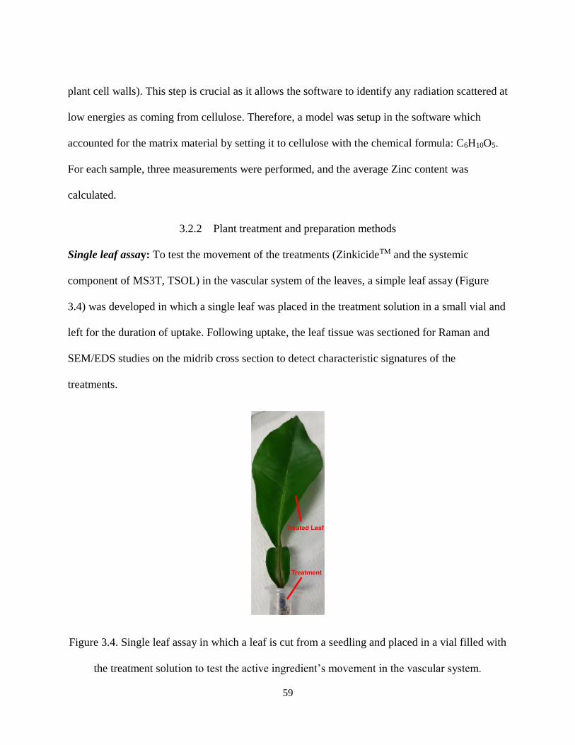
59

plant cell walls). This step is crucial as it allows the software to identify any radiation scattered at

low energies as coming from cellulose. Therefore, a model was setup in the software which

accounted for the matrix material by setting it to cellulose with the chemical formula: C6H10O5.

For each sample, three measurements were performed, and the average Zinc content was

calculated.

3.2.2 Plant treatment and preparation methods

Single leaf assay: To test the movement of the treatments (ZinkicideTM and the systemic

component of MS3T, TSOL) in the vascular system of the leaves, a simple leaf assay (Figure

3.4) was developed in which a single leaf was placed in the treatment solution in a small vial and

left for the duration of uptake. Following uptake, the leaf tissue was sectioned for Raman and

SEM/EDS studies on the midrib cross section to detect characteristic signatures of the

treatments.

Figure 3.4. Single leaf assay in which a leaf is cut from a seedling and placed in a vial filled with

the treatment solution to test the active ingredient’s movement in the vascular system.

60

Whole seedling assay to test root uptake of ZinkicideTM: Seedlings were removed from the soil

and the roots were cleaned, before being immersed in the treatment for a selected duration of

uptake. At timepoints 6 h, 12 h, 18 h, and 24 h, the seedlings were sectioned at different

locations for characterization. Figure 3.5 (a) shows the whole seedling assay setup. During

treatment, the seedlings were placed inside a growth chamber in order to simulate the field

conditions in Florida. The temperature of the growth chamber was set to cycle between 25 °C

and 31 °C, and the humidity was set to cycle between 60% and 80%. Day/night cycles were also

simulated.

Setup to test foliar uptake of MS3T and systemic component TSOL: The foliar uptake of MS3T

as well as the systemic Zn active TSOL alone was tested to compare the uptake with and without

the clay and Fixed quat components. Both treatments had a concentration of 1600 ppm metallic

Zn. The treatments were sprayed at a rate of two sprays per leaf (one spray at the top and one at

the bottom side of the leaf blade). After spraying, the seedlings were placed inside the growth

chamber to match the conditions in the field. The growth chamber settings were as outlined in

the previous section concerning root uptake of ZinkicideTM. The seedlings were left inside the

growth chamber for varying uptake durations: 2 h, 4 h, 6 h, 12 h, and 24 h. For each duration,

three seedlings were treated, in addition to three control untreated seedlings. Following uptake,

the plant leaves, stem, and roots from treated and untreated seedlings were washed in order to

remove any residues from the surface of the plant materials. After washing, the plant material

was left to dry in an oven at ~ 60 °C for 24 h. After drying, the plant material was ground into

fine powder.

61

Washing procedure: The washing protocol involved extensive cleaning of the leaves, stem, and

roots, to ensure removal of any residues remaining on the surface after foliar spray treatment

since our aim is to quantify the uptake of the treatments. First, the plant material is rinsed gently

in a mixture of 40 ml of 0.1% alconox in 2L of DI water. Next, the plant material is rinsed three

times in pure RO water, while ensuring the water is discarded in-between each step. The plant

tissue is then placed in 0.75M of HCL for 30 s prior to final rinsing in DI water204. Following

washing, the plants were left to dry overnight in oven at 60 °C.

Powder preparation for spectroscopy: Plant material was grinded into powder using a spice and

nut grinder. Each sample was grinded for an equal duration to homogenize the size of the pieces

in the powder (due to the lack of a Wiley mill).

FTIR measurement on plant tissue: FTIR measurement was performed on the powder samples.

For each sample, at least five spectra were acquired. PCA was performed on the data using a

specialized software (The Unscrambler X) following treatment of the data as follows: The FTIR

spectra were first converted from transmittance to absorbance spectra. Baseline adjustment and

mean normalization were then performed before PCA was run on the dataset.

Tissue sectioning for imaging: When uptake duration and washing (if necessary) were

completed, each seedling was cut into four segments (Figure 3.5 (b)).

SEM and EDS measurement on plant tissue: To perform the measurement, first the leaf blade

of four leaves obtained from the four segments was cut after flash freezing in liquid nitrogen to

preserve the conditions inside the leaf. The sections were then coated with gold-palladium using

a sputter-coater (Emitech K550) at 30 mA for 1 minute and 30 seconds. SEM imaging was done

62

with a 10 keV electron beam, a 60 μm electromagnetic lens aperture, and a 13 mm working

distance.

Figure 3.5. Setup for the uptake experiment. (a) Whole seedling assay setup. (b) The shoot part

of each seedling is divided into four segments. (c) Sectioning the leaf blade to obtain leaf extract.

3.3 Characterization of ZinkicideTM and MS3T

3.3.1 Characterization of ZinkicideTM

The initial formulation of ZinkicideTM investigated was pure research grade ZinkicideTM

chemicals, and henceforth is referred to as ZinkicideTM SG6. During the initial stages of the

project, ZinkicideTM SG6 was characterized using infrared spectroscopy (Raman spectroscopy,

FTIR) in order to identify the chemical signature of its main components. The individual

components and reagents used in synthesis were also tested to facilitate the assignment of the

characteristic Raman and IR bands observed.

63

The Raman spectra of ZinkicideTM SG6 (Figure 3.6 (a)) show characteristic bands at 810 cm-1,

870 cm-1, 1050 cm-1, 1260 cm-1, 1390 cm-1, and 1630 cm-1. The band at 810 cm-1 is attributed to

out of plane C-H deformations in sodium salicylate, which is used as a coating agent for the

nanoparticles in this formulation. Bands from sodium salicylate are also observed at 1260 cm-1

corresponding to benzene ring vibrations, 1390 cm-1 corresponding to symmetric carboxylic

group stretching, and 1630 cm-1 corresponding to asymmetric carboxylic group stretching205. The

band observed at 870 cm-1 is attributed to O-O stretching in hydrogen peroxide, while the band at

1050 cm-1 is attributed to N-O stretching vibrations in nitrate206.

More recently, a modified formulation suitable for industrial scale production was adopted and

dubbed ZinkicideTM TMN 110. This formulation was synthesized using agricultural grade

reagents; however, the composition is protected by proprietary information. Two versions of this

formulation were synthesized: TMN 110 and TMN 113. TMN 110 is the final agricultural grade

formulation for ZinkicideTM including all ingredients and reagents used in synthesis. TMN 113 is

excluding hydrogen peroxide. ZinkicideTM TMN 110 was characterized to identify its chemical

signature with a view to future studies of its uptake and effects inside citrus plants, in addition to

aging studies. The Raman bands corresponding to sodium salicylate(810 cm-1, 1020 cm-1, 1260

cm-1, 1390 cm-1, 1460 cm-1, 1630 cm-1, and 3070 cm-1), hydrogen peroxide (870 cm-1), and

nitrate (1050 cm-1) observed in ZinkicideTM SG6 are also observed in ZinkicideTM TMN 110

(Figure 3.6 (b)). The ratio of the peak intensity of hydrogen peroxide (870 cm-1) to the peak

intensity of nitrate (1050 cm-1) is significantly lower in ZinkicideTM TMN 110 than in

ZinkicideTM SG6. This suggests that a lower amount of hydrogen peroxide relative to nitrate is

used in the synthesis of ZinkicideTM TMN 110 compared to ZinkicideTM SG6.

64

FTIR spectra obtained from both ZinkicideTM SG6 and TMN 110 also show some differences

between the two formulations (Figure 3.7). Peaks assigned to sodium salicylate are observed at

740 cm-1, 810 cm-1, 860 cm-1, 980 cm-1, 1030 cm-1, 1480 cm-1, and 1580 cm-1 for ZinkicideTM

SG6 (Figure 3.7 (a)). Additionally, a strong broad band in the range of 1310 – 1380 cm-1 is

observed which corresponds to nitrate. Similar bands are observed in ZinkicideTM TMN 110

(Figure 3.7 (b)), but with shifts in peak positions. For example, the band at 740 cm-1

corresponding to out of plane C-H deformation in salicylate shifts to ~ 760 cm-1, and the band at

1580 cm-1 corresponding to asymmetric carboxyl group stretching in salicylate shifts to ~ 1550

cm-1. The band at 1480 cm-1 observed in ZinkicideTM SG6 is not present in ZinkicideTM TMN

110. The reason behind the shifts in peak positions as well as the disappearance of the band at

1480 cm-1 can be due to the fact that ZinkicideTM TMN 110 contains additional chemicals that

could be interacting with the salicylate groups. The composition of ZinkicideTM TMN 110 is

protected by proprietary information; however, the changes observed in FTIR and Raman spectra

can shed some light on how the ingredients interact with one another, and possibly on the

structure or defects present in the nanoparticles, which in turn can aid in optimizing the treatment

for best performance in the future. Full Raman and IR peak assignments are summarized in

Table 3.1.

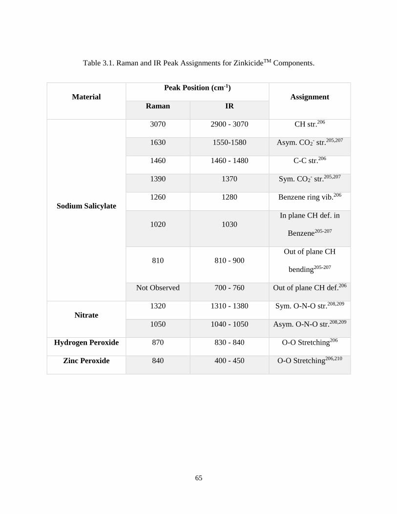
65

Table 3.1. Raman and IR Peak Assignments for ZinkicideTM Components.

Material

Peak Position (cm-1)

Assignment

Raman IR

Sodium Salicylate

3070 2900 - 3070 CH str.206

1630 1550-1580 Asym. CO2- str.205,207

1460 1460 - 1480 C-C str.206

1390 1370 Sym. CO2- str.205,207

1260 1280 Benzene ring vib.206

1020 1030

In plane CH def. in

Benzene205-207

810 810 - 900

Out of plane CH

bending205-207

Not Observed 700 - 760 Out of plane CH def.206

Nitrate

1320 1310 - 1380 Sym. O-N-O str.208,209

1050 1040 - 1050 Asym. O-N-O str.208,209

Hydrogen Peroxide 870 830 - 840 O-O Stretching206

Zinc Peroxide 840 400 - 450 O-O Stretching206,210

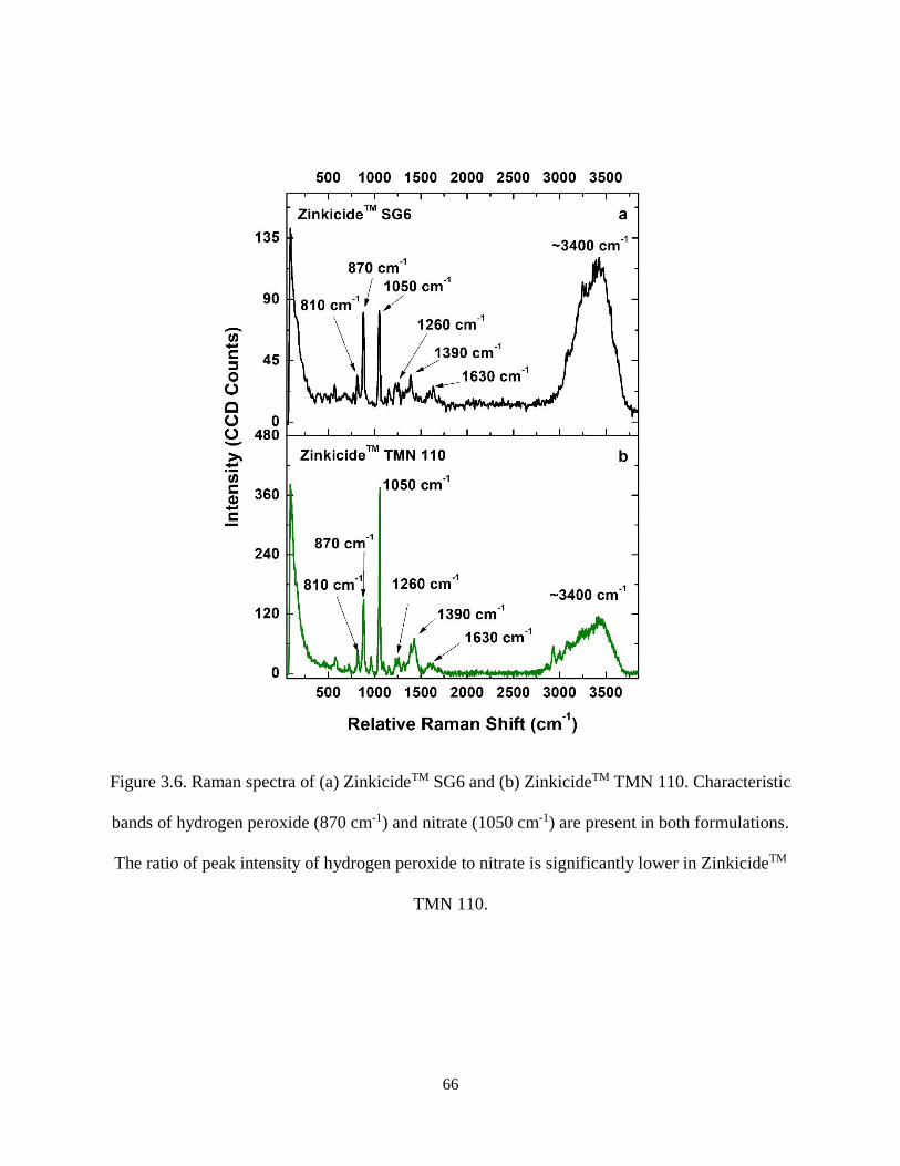
66

Figure 3.6. Raman spectra of (a) ZinkicideTM SG6 and (b) ZinkicideTM TMN 110. Characteristic

bands of hydrogen peroxide (870 cm-1) and nitrate (1050 cm-1) are present in both formulations.

The ratio of peak intensity of hydrogen peroxide to nitrate is significantly lower in ZinkicideTM

TMN 110.

67

Figure 3.7: FTIR spectra obtained from (a) ZinkicideTM SG6 and (b) ZinkicideTM TMN 110.

Significant variations in the IR spectra are observed between both formulations, for example the

band at 740 cm-1 in ZinkicideTM SG6 shifts to 760 cm-1 with a much lower intensity in

ZinkicideTM TMN 110.

68

ZinkicideTM TMN 110 and 113 were also studied using SEM imaging to observe their structures

at the nanoscale. (Figure 3.8). The SEM images highlight how one ingredient, hydrogen

peroxide, can affect the morphology of the aggregates at the nanoscale, with ZinkicideTM TMN

110 showing a round shape and ZinkicideTM TMN 113 showing a plate-like structure.

Figure 3.8. SEM images of (a) ZinkicideTM TMN 110 and (b) ZinkicideTM TMN 113 aggregates.

TMN 110 exhibited a round structure, whereas TMN 113 showed plate-like structures.

Aging study for ZinkicideTM SG6

Given that the formulations are meant to be stored for several months, we studied the stability

and potency of the formulations –nanoparticles aging in reagents or in water- over the course of

12 weeks. This was achieved by acquiring Raman spectra of the solutions on a weekly basis for a

period of 12 weeks. Figure 3.9 explains the set of solutions that were tested in the aging study

and are discussed here.

69

Figure 3.9. The solutions tested in the aging study for ZinkicideTM SG6. The solutions were

tested on a weekly basis including the original ZinkicideTM SG6 including the excess reagents, a

control with all ingredients except Zinc nitrate, a washed solution left to age in water from the

initial time point, and a washed solution that is obtained at each time point after aging in the

reagents. Each solution was shaken prior to obtaining 10 μL droplets for measurement.

The aging of ZinkicideTM SG6 was studied by monitoring the ratio of the intensities of hydrogen

peroxide (870 cm-1) and water (3400 cm-1) Raman bands in Raman spectra obtained from

ZinkicideTM SG6 aging in excess ingredients conditions. This ratio was chosen because of a

reduction in the hydrogen peroxide peak intensity (870 cm-1) observed in initial aging studies.

Raman spectra (Figure 3.8) of the solutions at the initial time point show the characteristic bands

of ZinkicideTM SG6 such as the hydrogen peroxide peak (870 cm-1) and the nitrate peak (1050

cm-1). The spectrum of washed ZinkicideTM SG6 shows a peak at 840 cm-1 which is attributed to

the O-O stretching vibration in Zinc Peroxide (ZnO2)210. The presence of this band suggests that

70

the nanoparticles not only consist of ZnO but also have a ZnO2 component which might have a

key role in the efficacy of the nanoparticles against HLB.

First we consider the aging of the ZinkicideTM SG6 formulation. Following the first 12 weeks,

the ratio of the peroxide peak (870 cm-1) to the water peak (~3400 cm-1) decreases from ~ 0.7 to

~ 0.55 in the ZinkicideTM SG6 formulation aging in the reagents (Figure 3.9). On the other hand,

the ratio of these peaks remains around 0.9 for the control solution. The measurement was

repeated after 18 weeks and shows further decay in the same ratio to ~ 0.4 in ZinkicideTM SG6,

and ~ 0.7 in the control solution. In terms of the washed solutions (Figure 3.12), the peak at 840

cm-1 corresponding to ZnO2 is present even at week 12 of the study for both the washed solution

aging in water (Figure 3.12 (a)) and the washed solution obtained after aging in the reagents

(Figure 3.12 (b)). A decay in the ratio of the ZnO2 peak (840 cm-1) to the water peak (3400 cm-1)

is observed from ~ 0.7 to ~ 0.4 by week 12 for the washed aging in water solution; nevertheless,

the measurement was repeated after 18 weeks and the ratio is found to be around 0.55 which

suggests that ZnO2 is fairly stable.

Overall, this type of study can help understand which ingredients of ZinkicideTM SG6 will be

stable over long storage periods. These results are also correlated to efficacy measurements

conducted on bacterial species such as E.Coli where the efficacy of the ZinkicideTM SG6 was

noted to decrease with time211. It is possible that the decay observed in the hydrogen peroxide

peak (870 cm-1) intensity is correlated with the reduction in efficacy; however, further

measurements are needed to confirm.

71

Figure 3.10. Raman spectra of ZinkicideTM SG6 (a), Washed ZinkicideTM SG6 (b), and the

control solution (c) at the initial time point of the aging study. ZinkicideTM SG6 exhibits

hydrogen peroxide (870 cm-1) and nitrate (1050 cm-1) peaks, whereas the washed solution

exhibits a Zn peroxide peak (840 cm-1).

0

47

94

141

0 500 1000 1500 2000 2500 3000 3500

0

27

54

81

0 500 1000 1500 2000 2500 3000 3500

0

45

90

135

1050 cm-1

870 cm-1

Zinkicide SG6 a

bWashed Zinkicide SG6

c

840 cm-1

Control Solution

870 cm-1In

ten

sit

y (

CC

D C

ou

nts

)

Relative Raman Shift (cm-1)

72

Figure 3.11. Evolution of hydrogen peroxide and ZinkicideTM SG6 with respect to water over

time. During the first 12 weeks, the ratio of the intensities of peroxide at ~870 cm-1 to water at

~3400 cm-1 decays over time in ZinkicideTM SG6, but stays fairly constant for the control

solution.

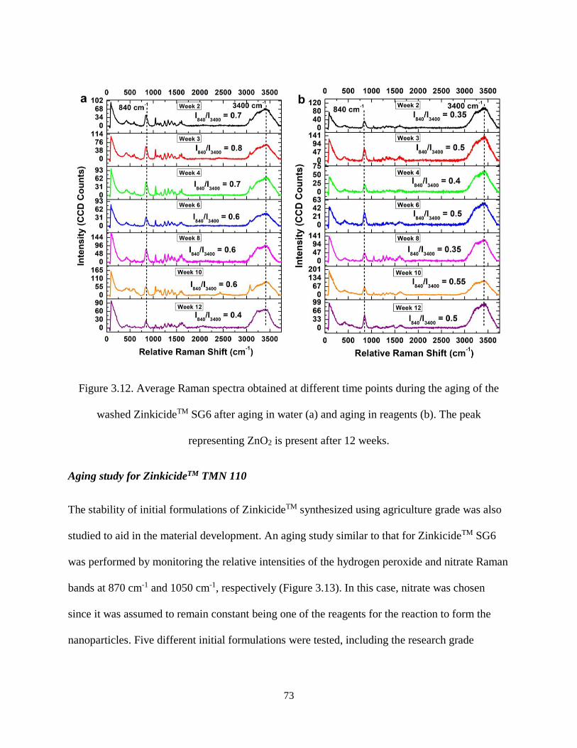
73

Figure 3.12. Average Raman spectra obtained at different time points during the aging of the

washed ZinkicideTM SG6 after aging in water (a) and aging in reagents (b). The peak

representing ZnO2 is present after 12 weeks.

Aging study for ZinkicideTM TMN 110

The stability of initial formulations of ZinkicideTM synthesized using agriculture grade was also

studied to aid in the material development. An aging study similar to that for ZinkicideTM SG6

was performed by monitoring the relative intensities of the hydrogen peroxide and nitrate Raman

bands at 870 cm-1 and 1050 cm-1, respectively (Figure 3.13). In this case, nitrate was chosen

since it was assumed to remain constant being one of the reagents for the reaction to form the

nanoparticles. Five different initial formulations were tested, including the research grade

74

ZinkicideTM SG6 (which is referred to as ZinkicideTM 1 in this study). Table 3.2 summarizes the

differences between each of the five formulations.

Table 3.2. Characteristics of the five formulations tested during the development of agricultural

grade ZinkicideTM.

Formulation pH Concentration

Zn (ppm) Peroxide

Rate

ZinkicideTM 1 6 50,000 1

ZinkicideTM 2 6 50,000 0.5

ZinkicideTM 3 6 20,000 1

ZinkicideTM 4 6 20,000 0.5

ZinkicideTM 5 7 50,000 1

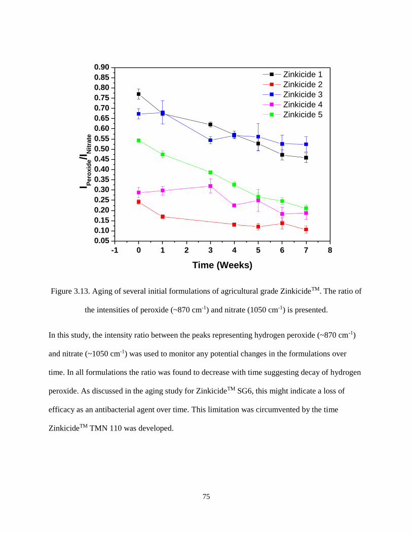
75

Figure 3.13. Aging of several initial formulations of agricultural grade ZinkicideTM. The ratio of

the intensities of peroxide (~870 cm-1) and nitrate (1050 cm-1) is presented.

In this study, the intensity ratio between the peaks representing hydrogen peroxide (~870 cm-1)

and nitrate (~1050 cm-1) was used to monitor any potential changes in the formulations over

time. In all formulations the ratio was found to decrease with time suggesting decay of hydrogen

peroxide. As discussed in the aging study for ZinkicideTM SG6, this might indicate a loss of

efficacy as an antibacterial agent over time. This limitation was circumvented by the time

ZinkicideTM TMN 110 was developed.

-1 0 1 2 3 4 5 6 7 8

0.05

0.10

0.15

0.20

0.25

0.30

0.35

0.40

0.45

0.50

0.55

0.60

0.65

0.70

0.75

0.80

0.85

0.90 Zinkicide 1

Zinkicide 2

Zinkicide 3

Zinkicide 4

Zinkicide 5

I Pero

xid

e/I

Nit

rate

Time (Weeks)

76

3.3.2 Characterization of MS3T and its Components

MS3T was designed with a vision to rapid deployment in the field due to the imminent threat of

wiping out citrus groves in Florida. The main components of MS3T (Clay, quaternary

ammonium compound (fixed quat), and TSOL (Zn-chelate active)) are already being used

separately in agriculture. Based on these considerations, MS3T should not require the time-

consuming process of EPA approval that is being enforced for ZinkicideTM. One of the goals of

the project is to study uptake of the active components of MS3T, and to investigate the effects on

citrus plants. Before starting the uptake studies, given that the structure of TSOL is not fully

understood, we monitored changes in the characteristic IR and Raman bands of the components

of TSOL (Zn nitrate, urea, and peroxide) to help in determining how these chemicals interact.

First, the individual components of MS3T were examined (Figure 3.14), and the FTIR spectrum

of clay exhibits distinct characteristic bands (Figure 3.14 (b)). For instance, the peaks at 3620-

3690 cm-1 are attributed to stretching vibrations of the inner hydroxyl (OH) groups lying between

the tetrahedral and octahedral layers212. Moreover, peaks observed at 1000 cm-1 and 1110 cm-1

are attributed to stretching vibrations of Si-O bonds206. Finally, the bands observed between 750

cm-1 and 990 cm-1 are attributed to metal OH bending vibrations, for example Al2OH bending212.

In the quaternary compound, the bands observed in the region of 2850 to 2920 cm-1 are attributed

to C-H stretching vibrations206, whereas the band observed at 1620 cm-1 is attributed to OH

bending206. The band observed at 1460 cm-1 is attributed to C-H bending and CH2 and CH3

deformation. In TSOL (Figure 3.14 (a)), the bands observed between 3260 cm-1 and 3440 cm-1

are attributed to N-H stretching vibrations as well as NH2 rocking206,213. These likely correspond

to urea in TSOL. Moreover, the band at 1620 cm-1 is attributed to OH bending, while the bands

77

observed between 1340 and 1380 cm-1 are attributed to the nitrate group206. Table 3.3

summarizes the peak assignments for MS3T and its individual components.

Table 3.3. Characteristic IR peak assignments for MS3T and its individual components.

FTIR Peak (cm-1) Peak Assignment

TSOL 1630 OH Bending206, NH vibration in Urea213

1460 C-N Stretching in Urea213

1310-1380 NO3- Stretching208,209

1160 C-N Stretching in Urea213

1050 NO3- Stretching208,209

Quat 2850-2950 C-H stretching and CH3 or CH2 deformations in methyl and decyl

groups206

1460 CH2 Scissor Vibration206

1380 Symmetric CH stretching in CH3 group (C-CH3)206

1290 CH2 Twisting Vibration206

950 CH3 Rocking Vibration206

750-810 CH2 Rocking Vibration206

Clay 3620-3690 Inner hydroxyl (OH) groups, lying between the tetrahedral and

octahedral sheets212

1000-1110 Si-O Stretching209

900-990 Al2OH bending212

MS3T 3620-3690 Inner hydroxyl (OH) groups, lying between the tetrahedral and

octahedral sheets in clay212

1340-1380 NO3- Stretching in TSOL208

1000-1110 Si-O bond in clay209

900-990 Al2OH bending in clay212

750-810 CH2 rocking in Quat206

78

Figure 3.14. FTIR spectra obtained from (a) TSOL, (b) clay, (c) quaternary compound, and (d)

MS3T. TSOL exhibits a strong broad peak at 1340-1380 cm-1 indicative of nitrate, as well as a

peak at ~1620 cm-1 corresponding to N-H vibrations in urea. MS3T exhibits peaks that can be

traced back to the individual components clay, quaternary compound, and TSOL.

79

Characterization of TSOL

TSOL is the active component of MS3T. In order to determine the structure of TSOL at the

molecular level, a titration experiment was designed to better understand the interaction of

peroxide, urea, and Zn nitrate to form TSOL. To understand the interactions, the following

binary compounds were tested: urea and hydrogen peroxide, urea and Zn nitrate, and Zn nitrate

and hydrogen peroxide, in addition to the TSOL formulation including all three components.

Figure 3.15 shows the fingerprint region of the FTIR spectra of TSOL, urea, urea and hydrogen

peroxide, and urea and Zn nitrate. The first observation is that the FTIR spectrum of TSOL

closely matches that of urea and Zn nitrate, which shows that urea and Zn form a complex inside

TSOL. Additionally, we observed that the C-N asymmetric stretch band in urea (~1460 cm-1)

shifts to higher frequencies in TSOL, while the C=O group in urea (~1680 cm-1) shifts to lower

frequencies in TSOL. This confirms that the Zn metal is binding to the oxygen atom in the

carbonyl group in the Zn-urea complex formed in TSOL214. The similarity between the spectra of

pure urea and urea-peroxide suggests that little or no interaction takes place between the two

components. In order to further explore the structure of TSOL and extract the most information

from the IR spectra, modeling and simulation of the molecular structure of TSOL was performed

by Dr. Loukas Petridis’ group at University of Tennessee and the Oak Ridge National

Laboratory215.

80

Figure 3.15. FTIR spectra of urea (U), urea and Zn nitrate (U+ZN), urea and hydrogen peroxide

(U+P), and TSOL. The IR spectra for TSOL and urea and Zn nitrate show shifts in the bands

corresponding to C=O and N-C-N vibrations in urea compared to the IR spectrum of urea.

To corroborate the results of FTIR, a titration experiment was designed in which the

concentration of one of TSOL’s constituents was varied (Figure 3.16). Five different solutions of

TSOL were prepared with different concentrations of Zn nitrate. The concentrations (urea :

hydrogen peroxide : Zn nitrate) were as follows 1:1:0.1, 1:1:0.2, 1:1:0.5, 1:1:0.7, and 1:1:1.

Raman spectra were acquired for each solution as described previously.

81

Figure 3.16. Raman spectra of the different solutions of Zn nitrate and urea used in the titration

experiment. As the concentration of Zn nitrate increases, the peak at 1010 cm-1 corresponding to

N-C-N stretching in urea shifts to higher frequencies.

Previous studies213,214,216 of metal-urea complexes have shown that when the C-N band shifts to

higher frequencies, the metal binds to the oxygen of the carbonyl group in urea. As can be seen

in the Raman spectra shown in Figure 3.16, with increasing Zn nitrate content, the peak for

symmetric stretching of N-C-N stretching resulting from urea shifts from ~1010 cm-1 at a Zn

nitrate to urea ratio of 0.1 to ~1025 cm-1 at a ratio of 1. This shift to a higher frequency indicates

that Zn forms a complex with urea in TSOL where it binds to the oxygen atom in the carbonyl

group216.

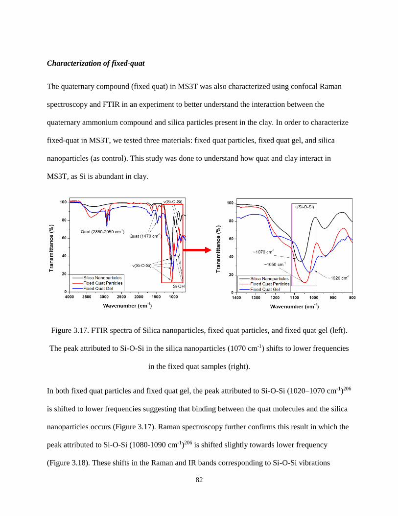
82

Characterization of fixed-quat

The quaternary compound (fixed quat) in MS3T was also characterized using confocal Raman

spectroscopy and FTIR in an experiment to better understand the interaction between the

quaternary ammonium compound and silica particles present in the clay. In order to characterize

fixed-quat in MS3T, we tested three materials: fixed quat particles, fixed quat gel, and silica

nanoparticles (as control). This study was done to understand how quat and clay interact in

MS3T, as Si is abundant in clay.

Figure 3.17. FTIR spectra of Silica nanoparticles, fixed quat particles, and fixed quat gel (left).

The peak attributed to Si-O-Si in the silica nanoparticles (1070 cm-1) shifts to lower frequencies

in the fixed quat samples (right).

In both fixed quat particles and fixed quat gel, the peak attributed to Si-O-Si (1020–1070 cm-1)206

is shifted to lower frequencies suggesting that binding between the quat molecules and the silica

nanoparticles occurs (Figure 3.17). Raman spectroscopy further confirms this result in which the

peak attributed to Si-O-Si (1080-1090 cm-1)206 is shifted slightly towards lower frequency

(Figure 3.18). These shifts in the Raman and IR bands corresponding to Si-O-Si vibrations

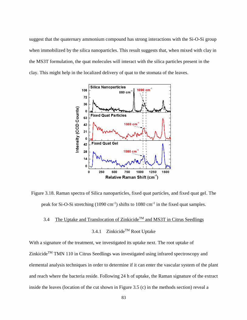
83

suggest that the quaternary ammonium compound has strong interactions with the Si-O-Si group

when immobilized by the silica nanoparticles. This result suggests that, when mixed with clay in

the MS3T formulation, the quat molecules will interact with the silica particles present in the

clay. This might help in the localized delivery of quat to the stomata of the leaves.

Figure 3.18. Raman spectra of Silica nanoparticles, fixed quat particles, and fixed quat gel. The

peak for Si-O-Si stretching (1090 cm-1) shifts to 1080 cm-1 in the fixed quat samples.

3.4 The Uptake and Translocation of ZinkicideTM and MS3T in Citrus Seedlings

3.4.1 ZinkicideTM Root Uptake

With a signature of the treatment, we investigated its uptake next. The root uptake of

ZinkicideTM TMN 110 in Citrus Seedlings was investigated using infrared spectroscopy and

elemental analysis techniques in order to determine if it can enter the vascular system of the plant

and reach where the bacteria reside. Following 24 h of uptake, the Raman signature of the extract

inside the leaves (location of the cut shown in Figure 3.5 (c) in the methods section) reveal a

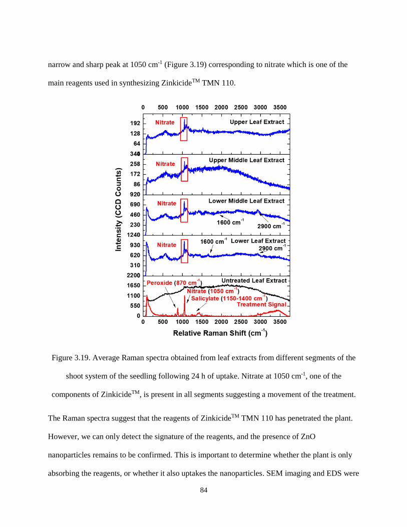
84

narrow and sharp peak at 1050 cm-1 (Figure 3.19) corresponding to nitrate which is one of the

main reagents used in synthesizing ZinkicideTM TMN 110.

Figure 3.19. Average Raman spectra obtained from leaf extracts from different segments of the

shoot system of the seedling following 24 h of uptake. Nitrate at 1050 cm-1, one of the

components of ZinkicideTM, is present in all segments suggesting a movement of the treatment.

The Raman spectra suggest that the reagents of ZinkicideTM TMN 110 has penetrated the plant.

However, we can only detect the signature of the reagents, and the presence of ZnO

nanoparticles remains to be confirmed. This is important to determine whether the plant is only

absorbing the reagents, or whether it also uptakes the nanoparticles. SEM imaging and EDS were

85

used to evaluate the elemental composition of the plant tissues (phloem and xylem). EDS spectra

(Figure 3.20) reveal a peak at 1.01 keV in treated plants that is not present in untreated control.

The peak at 1.01 keV correspond to the Lα transition in Zn217. Based on this, we could further

investigate the composition of the xylem and phloem using SEM images and EDS localized

spectra. We tested leaf midrib (Figure 3.20 (a)) and stem (Figure 3.20 (b)) cross sections

obtained from all four levels of the seedlings following 24 h of uptake and found that the Zn

peak at 1.01 keV is present in both the xylem and the phloem tissue of the leaf midrib (Figure

3.20 (c)) and stem (Figure 3.20 (d)) sections. In certain locations, a peak at ~ 2-2.1 keV was

observed, which corresponds to Kα or Kβ transitions in phosphorus (P)217. The fact that the peak

is observed in certain parts but not in others could be due to the localized nature of the

measurement and the accumulation of phosphorus in certain parts of the plant218.

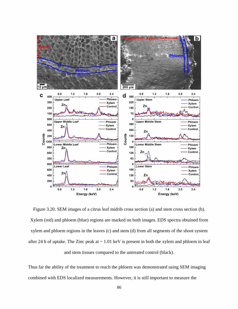
86

Figure 3.20. SEM images of a citrus leaf midrib cross section (a) and stem cross section (b).

Xylem (red) and phloem (blue) regions are marked on both images. EDS spectra obtained from

xylem and phloem regions in the leaves (c) and stem (d) from all segments of the shoot system

after 24 h of uptake. The Zinc peak at ~ 1.01 keV is present in both the xylem and phloem in leaf

and stem tissues compared to the untreated control (black).

Thus far the ability of the treatment to reach the phloem was demonstrated using SEM imaging

combined with EDS localized measurements. However, it is still important to measure the

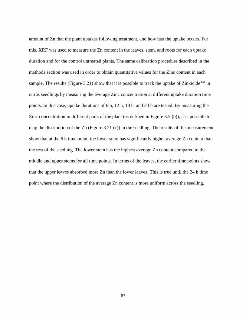
87

amount of Zn that the plant uptakes following treatment, and how fast the uptake occurs. For

this, XRF was used to measure the Zn content in the leaves, stem, and roots for each uptake

duration and for the control untreated plants. The same calibration procedure described in the

methods section was used in order to obtain quantitative values for the Zinc content in each

sample. The results (Figure 3.21) show that it is possible to track the uptake of ZinkicideTM in

citrus seedlings by measuring the average Zinc concentration at different uptake duration time

points. In this case, uptake durations of 6 h, 12 h, 18 h, and 24 h are tested. By measuring the

Zinc concentration in different parts of the plant (as defined in Figure 3.5 (b)), it is possible to

map the distribution of the Zn (Figure 3.21 (c)) in the seedling. The results of this measurement

show that at the 6 h time point, the lower stem has significantly higher average Zn content than

the rest of the seedling. The lower stem has the highest average Zn content compared to the

middle and upper stems for all time points. In terms of the leaves, the earlier time points show

that the upper leaves absorbed more Zn than the lower leaves. This is true until the 24 h time

point where the distribution of the average Zn content is more uniform across the seedling.

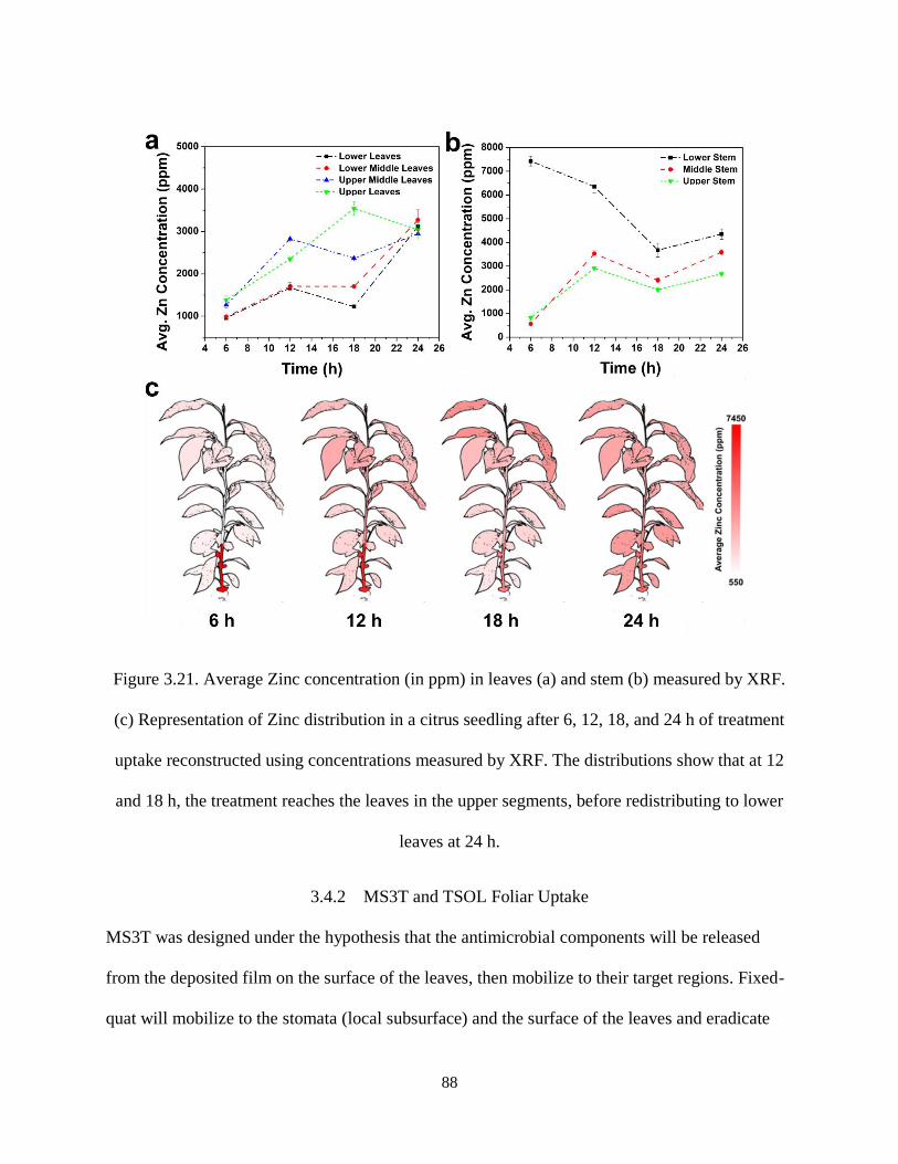
88

Figure 3.21. Average Zinc concentration (in ppm) in leaves (a) and stem (b) measured by XRF.

(c) Representation of Zinc distribution in a citrus seedling after 6, 12, 18, and 24 h of treatment

uptake reconstructed using concentrations measured by XRF. The distributions show that at 12

and 18 h, the treatment reaches the leaves in the upper segments, before redistributing to lower

leaves at 24 h.

3.4.2 MS3T and TSOL Foliar Uptake

MS3T was designed under the hypothesis that the antimicrobial components will be released

from the deposited film on the surface of the leaves, then mobilize to their target regions. Fixed-

quat will mobilize to the stomata (local subsurface) and the surface of the leaves and eradicate

89

microorganisms residing in these areas, while TSOL will mobilize systemically to the phloem

and kill CLas, eventually metabolizing into useful plant nutrients. As a result, it is critical to

understand the uptake and translocation of TSOL inside the plant following foliar spray of MS3T

to confirm the hypothesis outlined above. To achieve this, the foliar uptake of MS3T and active

ingredient TSOL was studied using IR spectroscopy (FTIR) and elemental analysis techniques

(EDS and XRF).

Prior to analyzing the treatment uptake and effects, the residue of sprayed MS3T was studied on

the surface of the leaf by SEM imaging and EDS mapping. Figure 3.22 (a) and (b) are SEM

images of untreated and treated leaf surfaces, respectively. As shown in Figure 3.22 (b), MS3T

forms aggregates on the surface of the leaf which cover the stomata. Figure 3.22 (c) shows

smaller MS3T aggregates penetrating a stomatal opening, which suggests that stomata constitute

an important path for uptake of the treatment. Elemental analysis was performed and confirms

the composition of the features observed (data not shown here).

90

Figure 3.22 SEM Imaging of MS3T deposited on the leaf surface after spraying. (a) Untreated

leaf surface showing stomatal openings. (b) MS3T aggregates forming on the leaf surface. (c)

MS3T aggregates can penetrate the stomatal opening.

91

The foliar uptake of MS3T and TSOL (systemic Zn active) in citrus seedlings was first

investigated using infrared spectroscopy to monitor the effect of the treatment and to determine

whether we can detect its characteristic IR bands inside the plant tissues. The mean normalized

FTIR spectra (Figure 3.23) exhibit IR bands that are attributed to the natural components of the

leaves. The peaks observed at 1010 cm-1 and 1160 cm-1 are attributed to C-O-C stretching

vibrations in cellulose219,220. The peak at 1100 cm-1 can be attributed to C-O stretching in

cellulose and hemicellulose219. The peaks at 1515 cm-1, and 1600 cm-1 can be attributed to C=C

and C-O stretching, respectively, in lignin219,221,222. The peak at 1730 cm-1 is attributed to C=O in

hemicellulose220. The IR spectra alone show a possible variation at 1410 cm-1, attributed to C-H

vibrations in cellulose and lignin, where the peak seems to be inhibited in TSOL and MS3T

treated leaves after 12 h (Figure 3.23 (a)) and 24 h (Figure 3.23 (b)) of treatment, which suggests

an effect of the treatment on the natural biopolymers of the plant.

Figure 3.23. Average mean normalized FTIR spectra obtained from untreated control leaves,

TSOL treated leaves, and MS3T treated leaves at (a) 12 h, and (b) 24 h time points. The peak at

1410 cm-1 has a higher intensity in the untreated leaves than in TSOL or MS3T at 12 h and 24 h.

92

To validate the observations made in the FTIR spectra of the untreated and treated leaves, PCA

was performed on the FTIR dataset. The results show that there is separation in the scores plot

along the first principal component (PC 1) between treated and untreated leaves (Figure 3.24

(a)). PC 1 is responsible for 61% of variation in the 12 h time point data, and 42% of variation in

the 24 h time point data. PC 1 loadings for both 12 h (Figure 3.24 (b)) and 24 h (Figure 3.24 (d))

treated leaves show significant variation in the bands at ~1010 cm-1 (corresponding to C-O-C

stretching in cellulose) as well as ~1410 cm-1 (corresponding to C-H bending in cellulose and

lignin). The results suggest that: 1) The treatment is uptaken by the leaves, or 2) The treatment is

influencing the components of the plant cell wall inside the leaves. This necessitates further

studies into the potential effects the treatments have on the plant. Separation between treated and

untreated leaves was observed in the scores plots after 12 h (Figure 3.24 (a)) and 24 h (Figure

3.24 (b)) treatments, although the difference at 24 h is less significant. This will require further

investigation.

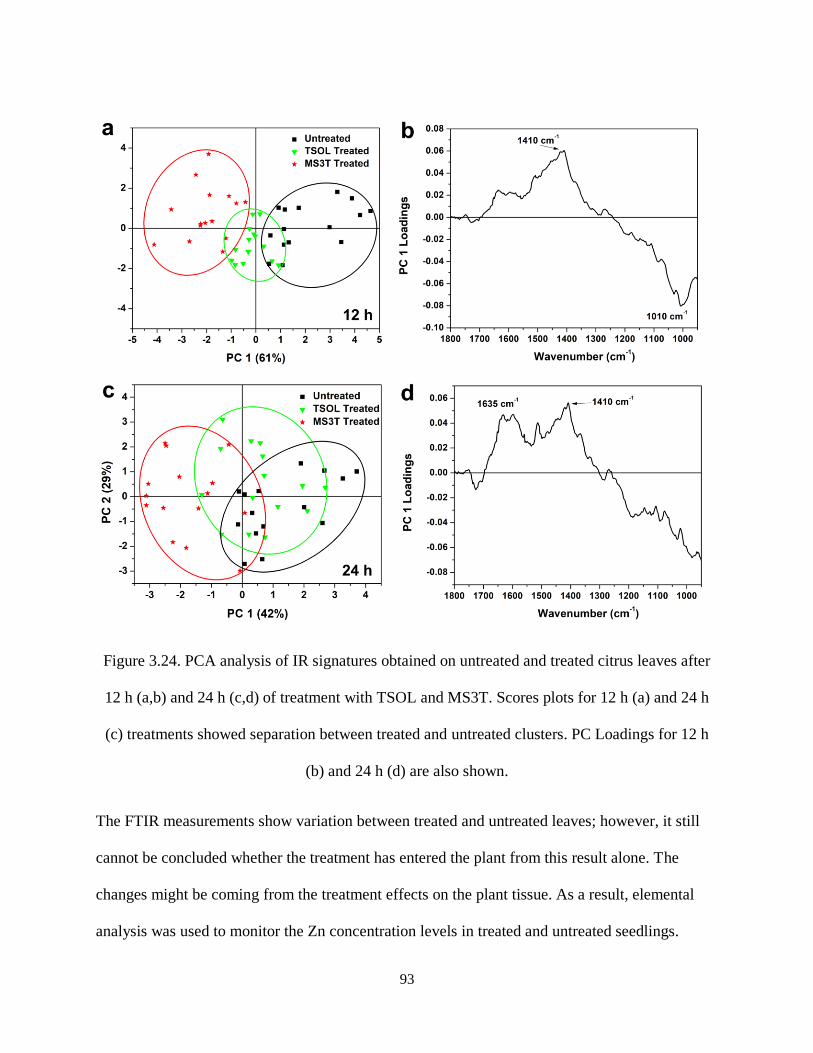
93

Figure 3.24. PCA analysis of IR signatures obtained on untreated and treated citrus leaves after

12 h (a,b) and 24 h (c,d) of treatment with TSOL and MS3T. Scores plots for 12 h (a) and 24 h

(c) treatments showed separation between treated and untreated clusters. PC Loadings for 12 h

(b) and 24 h (d) are also shown.

The FTIR measurements show variation between treated and untreated leaves; however, it still

cannot be concluded whether the treatment has entered the plant from this result alone. The

changes might be coming from the treatment effects on the plant tissue. As a result, elemental

analysis was used to monitor the Zn concentration levels in treated and untreated seedlings.

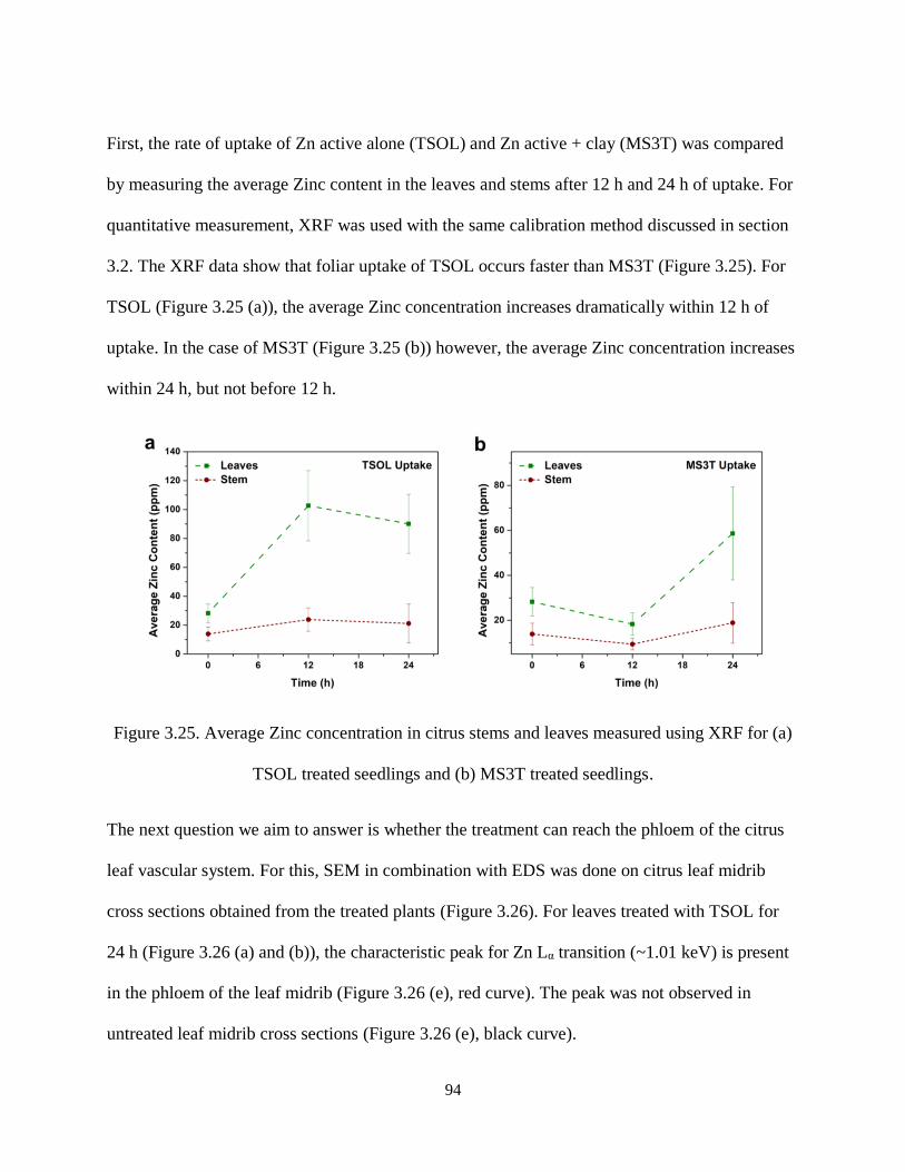
94

First, the rate of uptake of Zn active alone (TSOL) and Zn active + clay (MS3T) was compared

by measuring the average Zinc content in the leaves and stems after 12 h and 24 h of uptake. For

quantitative measurement, XRF was used with the same calibration method discussed in section

3.2. The XRF data show that foliar uptake of TSOL occurs faster than MS3T (Figure 3.25). For

TSOL (Figure 3.25 (a)), the average Zinc concentration increases dramatically within 12 h of

uptake. In the case of MS3T (Figure 3.25 (b)) however, the average Zinc concentration increases

within 24 h, but not before 12 h.

Figure 3.25. Average Zinc concentration in citrus stems and leaves measured using XRF for (a)

TSOL treated seedlings and (b) MS3T treated seedlings.

The next question we aim to answer is whether the treatment can reach the phloem of the citrus

leaf vascular system. For this, SEM in combination with EDS was done on citrus leaf midrib

cross sections obtained from the treated plants (Figure 3.26). For leaves treated with TSOL for

(~1.01 keV) is present transition αn Lfor Z , the characteristic peak(a) and (b)) 6(Figure 3.2 24 h

in the phloem of the leaf midrib (Figure 3.26 (e), red curve). The peak was not observed in

untreated leaf midrib cross sections (Figure 3.26 (e), black curve).

95

Figure 3.26. SEM images of treated and untreated leaf midrib cross sections. (a) Treated leaf

midrib cross section. (b) Higher resolution SEM image of the treated leaf midrib cross section

(marked by square in (a)), highlighting regions where EDS measurements were taken (marked by

squares). (c) Untreated leaf midrib cross section. (d) Higher resolution image of the untreated

leaf midrib cross section (marked by square in (c)), crosses mark regions where EDS

measurements were acquired. (e) Average EDS spectra obtained from treated (red) and untreated

(black) leaves to determine the presence of Zn (1.01 keV).

96

3.5 Summary

Plant diseases constitute a significant threat to food production at a time when world population

growth and economic development necessitate more efficient and sustainable efforts in

agriculture. Food availability and security is a major component of the food energy water nexus,

and tackling the issue of rapidly spreading plant diseases is one of the major ways of

supplementing the food sector.

In this chapter we focused on citrus greening disease, which is a systemic bacterial infection

threatening citrus crops in Florida and other regions around the world with extinction. We

examined two Zinc-based treatments developed for systemic activity, and demonstrated the

uptake and the effects these treatments can have on citrus seedlings. For example, the molecular

structure of the Zn active in MS3T was studied using infrared spectroscopy and our results

indicate that the Zn ions bind to the oxygen atom in the carbonyl group in urea to form a Zn-urea

complex which can be linked to its antibacterial activity.

The uptake and translocation of ZinkicideTM and MS3T is also studied using a protocol that

combines infrared spectroscopy with elemental analysis techniques. We confirmed that the

treatments can enter the plants through infrared spectroscopy techniques. We also demonstrated

how fast the plants uptake the treatments through quantitative measurements of the average Zn

content at different uptake durations using XRF. Finally, we proved that the active ingredients of

ZinkicideTM and MS3T can reach the phloem where the pathogens responsible for HLB reside by

combining SEM imaging with localized EDS measurements. This protocol combining multiscale

characterization methods has the potential to aid future growers in designing efficient field

application plans for novel treatments designed to overcome plant diseases and boost crop yields.

97

Several questions remain unanswered, however. The form that the treatments take inside the

plant remains unknown, particularly for ZinkicideTM where it is important to know whether the

Zn signal detected is coming from Zn2+ ions or the ZnO nanoparticles. It is also important to

study the fate of the treatments following uptake: do they accumulate inside the plants, or do

they decay with time? This is significant in terms of the safety to consume treated agricultural

products. Currently, field trials of MS3T and TSOL are underway to answer this question.

Overall, this research is highly impactful in terms of sustainable agriculture as it aids in

developing efficient treatments to combat plant diseases and enhance the efficiency of

agricultural production to meet the demands of a growing world population and a rapidly

developing world economy.

98

4 UTILIZING EXTERNAL STRESSES IN PLANTS FOR BIOMASS

VALORIZATION – THE EXAMPLES OF BIOMASS FILMS AND

GROWTH PROMOTERS

4.1 Background

Valorization of biomass is an increasingly growing field with the aim of putting waste and

biomass processing byproducts into use in the synthesis of new carbon materials that are

independent of the oil industry67,223,224. The oil industry is currently the main source where

chemical manufacturers obtain raw materials for synthesis of carbon-based products (plastics,

toothpaste, tires, etc.)67. Due to the impact on the environment, as well as rising costs and

declining supply, it is important to find alternative sources for the raw materials that sustain these

industries. As such, valorization of biomass waste into raw materials for these industries is

quickly becoming a promising method to fill the role of petroleum.

We have illustrated in chapters 2 and 3 that the structure and composition of plants can

significantly change when they are experiencing mechanical (chapter 2) and chemical (chapter 3)

stresses. Hence, it seems acceptable to envision utilizing these concepts to move toward

engineering of plants for future valorization of products from plant-derived materials. Such an

endeavor would require careful design and engineering to obtain the desired effects in the plants.

Mechanically stressed plants which exhibit favorable cellulose/lignin content for processing are a

promising system. A previous study in which tension wood was induced by letting plants grow at

a 45° angle, has already shown that it is possible to improve yield of glucose obtained by enzyme

saccharification of the biomass using this approach225. Improving the yield of cellulose

conversion to glucose constitutes a significant step in making biofuel extraction from plants a

more energy efficient process.

99

A significant part of improving cost effectiveness of biofuel production is the conversion of the

biomass byproducts of the biorefining process into useful high-value products. This would

constitute a major advance in developing a viable industry to reduce our current reliance on

fossil fuels and instead focus on renewable biofuel226. Examples of high value products that can

be obtained from biomass include chemicals223,224,227,228, carbon nanomaterials229,230, carbon

fibers231, and biomass films232.

Chemical stresses are often perceived as having negative effects on plants; however, if utilized in

a controlled way, chemical treatments could increase crop yields and achieve more efficient

agricultural production. The most common chemical treatment, nutritious fertilizers, has already

shown significant increases in crop yields in recent decades143,147. Nanoparticle-based treatments

also show promise as inducers of chemical stress in plants to improve crop yield by enhancing

plant growth15,17,18. Figure 4.1 shows how more value can be obtained from agricultural products

whether in terms of food production or energy and added value products.

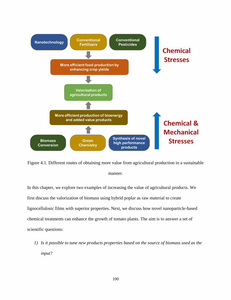
100

Figure 4.1. Different routes of obtaining more value from agricultural production in a sustainable

manner.

In this chapter, we explore two examples of increasing the value of agricultural products. We

first discuss the valorization of biomass using hybrid poplar as raw material to create

lignocellulosic films with superior properties. Next, we discuss how novel nanoparticle-based

chemical treatments can enhance the growth of tomato plants. The aim is to answer a set of

scientific questions:

1) Is it possible to tune new products properties based on the source of biomass used as the

input?

101

2) How does changing the solvent used in processing affect the composition of the

properties of the final product?

3) Can we enhance food production using nanoparticle-based chemical treatments?

A set of characterization tools are used to answer these questions including Confocal Raman

Mapping and advanced AFM-based methods such as Pulsed Force Mode AFM (PFM) (see the

methods part in section 4.2) and nanoscale infrared spectroscopy (nanoIR).

4.2 Example 1: Biomass Films Produced from Lignocellulosic Biomass

4.2.1 Methods

Deconstruction and Processing:

Biomass films were synthesized at the Center for Renewable Carbon, University of Tennessee,

Knoxville, Tennessee. After obtaining autohydrolyzed hybrid poplar by extracting the raw

biomass (187 g) with DI water at 160 °C for 60 min in a Hastelloy C276 pressure reactor, the

extracted material was dried at 40 °C until constant moisture was achieved, then milled using a

Wiley mill equipped with a 40-mesh screen. The powder material was then dissolved in an ionic

liquid (IL) ([C2mim][OAc]) by mechanically stirring at 100 °C in a 500 mL round bottle until

total dissolution. Following dissolution, the film was created by directly casting from the

solution while maintaining a temperature of 100 °C. Following casting, the films were

submerged in a coagulant bath three consecutive times to completely remove the ionic liquid

solvent. Three different types of coagulants were used: water, methanol, and a 50/50 by volume

mixture of DMAc and water. A full description of the synthesis method can be found in the

publication by Wang et al.232.

102

The main results of Wang et al. study are that the physicochemical properties of the films depend

on the coagulant solvent used, and that this is due primarily to the solubility parameters of these

solvents. The methanol film shows the highest Young’s modulus as well as tensile strength

which is attributed to having the ideal compositional ratio of carbohydrates to lignin. Methanol

films also exhibit homogeneous properties primarily due to slower diffusion of the ionic liquid

used during immersion in the coagulant bath compared to DMAc/water and water. Overall, the

results underline the promise of regenerating biomass films in a sustainable manner with

significant implications to manufacturing of green biomaterials with properties that match or

surpass current materials manufactured using synthetic non-biodegradable sources.

In this context, the measurements presented in the coming parts constitute a further step in

analyzing the nanomechanical properties in order to gain a deeper understanding of how the

processing parameters affect the final properties of these films.

Characterization Methods:

Pulsed Force Mode Atomic Force Microscopy (PFM):

PFM measurements were performed on a WITec Alpha 300 RA system. A cantilever with force

constant of ~5 N/m (Mikromasch 14-series) is mounted on the AFM holder to perform the force

distance measurements. In PFM, a force distance (or force time) curve is acquired at each point

as the probe scans the sample. Figure 4.2 shows a typical force time curve obtained in this

measurement. The slope of the curve is directly related to the stiffness of the sample at the point

where the curve is obtained. Other information such as adhesion and the maximum force

between the tip and the sample can be obtained from the curve as well.

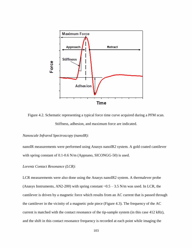
103

Figure 4.2. Schematic representing a typical force time curve acquired during a PFM scan.

Stiffness, adhesion, and maximum force are indicated.

Nanoscale Infrared Spectroscopy (nanoIR):

nanoIR measurements were performed using Anasys nanoIR2 system. A gold coated cantilever

with spring constant of 0.1-0.6 N/m (Appnano, SICONGG-50) is used.

Lorentz Contact Resonance (LCR):

LCR measurements were also done using the Anasys nanoIR2 system. A thermalever probe

(Anasys Instruments, AN2-200) with spring constant ~0.5 – 3.5 N/m was used. In LCR, the

cantilever is driven by a magnetic force which results from an AC current that is passed through

the cantilever in the vicinity of a magnetic pole piece (Figure 4.3). The frequency of the AC

current is matched with the contact resonance of the tip-sample system (in this case 412 kHz),

and the shift in this contact resonance frequency is recorded at each point while imaging the

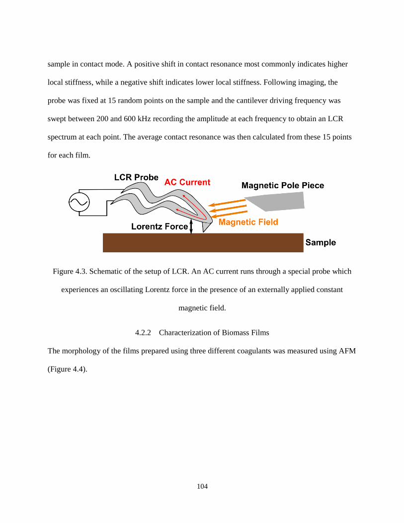
104

sample in contact mode. A positive shift in contact resonance most commonly indicates higher

local stiffness, while a negative shift indicates lower local stiffness. Following imaging, the

probe was fixed at 15 random points on the sample and the cantilever driving frequency was

swept between 200 and 600 kHz recording the amplitude at each frequency to obtain an LCR

spectrum at each point. The average contact resonance was then calculated from these 15 points

for each film.

Figure 4.3. Schematic of the setup of LCR. An AC current runs through a special probe which

experiences an oscillating Lorentz force in the presence of an externally applied constant

magnetic field.

4.2.2 Characterization of Biomass Films

The morphology of the films prepared using three different coagulants was measured using AFM

(Figure 4.4).

105

Figure 4.4. AFM topography images of films prepared using methanol (a,d), DMAc/water (b,e),

and water (c,f) as coagulants. Figure adapted from Wang et al.232.

The AFM images show significant variation in morphology between the films, with those

prepared using methanol and DMAc/water exhibiting globular-like structures. PFM was used to

test the stiffness and adhesion properties and identify any differences between the three films. In

this measurement, images of 20x20 μm size and 512 x 512 points were acquired; therefore, a

total of 262,144 points were tested on each film. The distribution of stiffness values obtained

from the three films shows significant variation between the three (Figure 4.5 (a)), with the

DMAc/water film having the highest stiffness, followed by the methanol film with a narrow

stiffness distribution, and the water film having the lowest stiffness. The average force curve for

each film was also plotted (Figure 4.5 (b)), and shows that the adhesion properties varied with

the water and DMAc/water films being significantly more hydrophilic than the methanol film.

This is in agreement with Hansen solubility data discussed by Wang et al.232. The PFM

106

measurements illustrate how changing one parameter of the processing conditions for the films,

in this case the coagulant used to remove the ionic liquid solvent, can drastically alter the

properties of the product obtained. This in turn shows the potential for materials design in

biomass valorization leading to a wide range of applications. For instance, UV-vis spectroscopy

measurements showed that the water films absorbed strongly in the UV range which could make

them potentially useful in applications which require protection from UV radiation232.

Figure 4.5. (a) Distribution of stiffness values obtained from the PFM measurements. (b)

Representative PFM force curves for water (black), methanol (red) and DMAC/water (blue)

films with the adhesion indicated in the red square.

In addition, when monitoring the frequency shift of the cantilever contact resonance with LCR,

one can observe some differences in the mechanical properties of the films (Figure 4.6 (d-f)).

The methanol films show the smallest domains and relatively smaller variation in the contact

resonance frequency between the domains (Figure 4.6 (d)). This is in agreement with

complementary results obtained by Wang et al232.

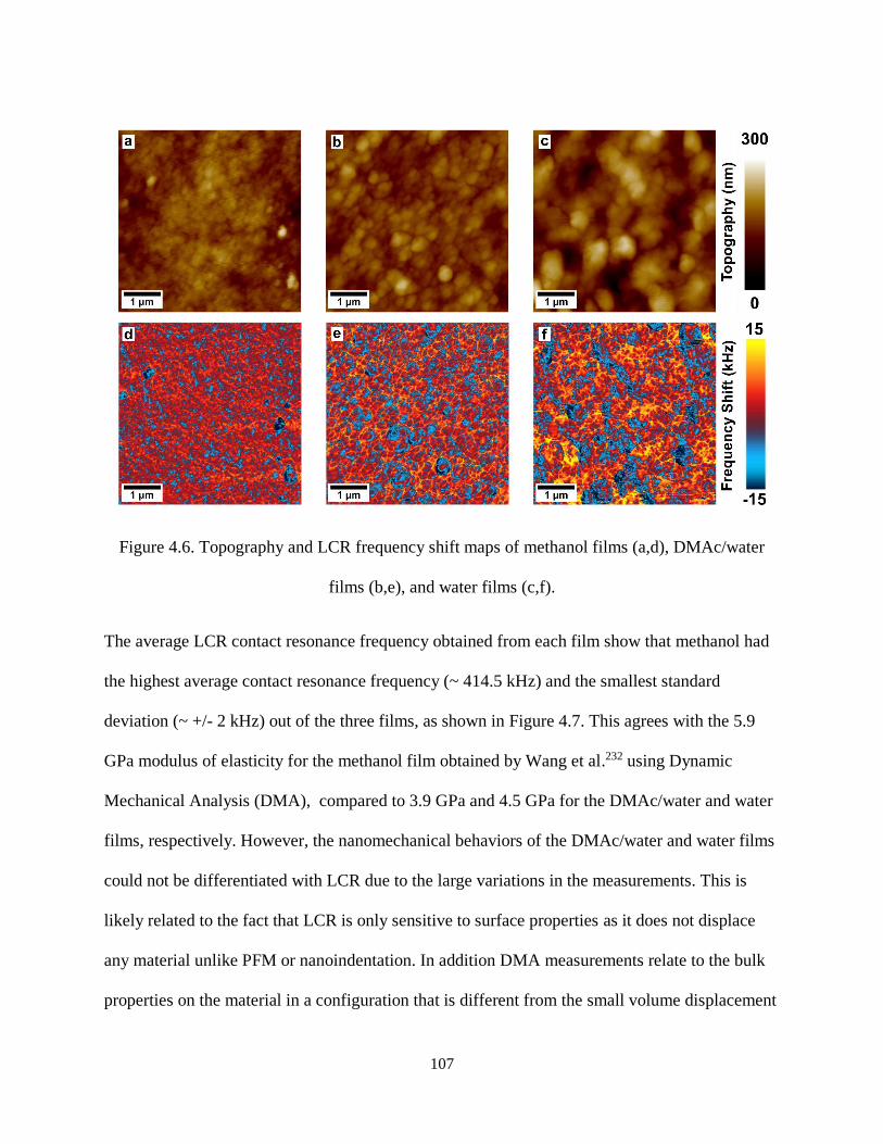
107

Figure 4.6. Topography and LCR frequency shift maps of methanol films (a,d), DMAc/water

films (b,e), and water films (c,f).

The average LCR contact resonance frequency obtained from each film show that methanol had

the highest average contact resonance frequency (~ 414.5 kHz) and the smallest standard

deviation (~ +/- 2 kHz) out of the three films, as shown in Figure 4.7. This agrees with the 5.9

GPa modulus of elasticity for the methanol film obtained by Wang et al.232 using Dynamic

Mechanical Analysis (DMA), compared to 3.9 GPa and 4.5 GPa for the DMAc/water and water

films, respectively. However, the nanomechanical behaviors of the DMAc/water and water films

could not be differentiated with LCR due to the large variations in the measurements. This is

likely related to the fact that LCR is only sensitive to surface properties as it does not displace

any material unlike PFM or nanoindentation. In addition DMA measurements relate to the bulk

properties on the material in a configuration that is different from the small volume displacement

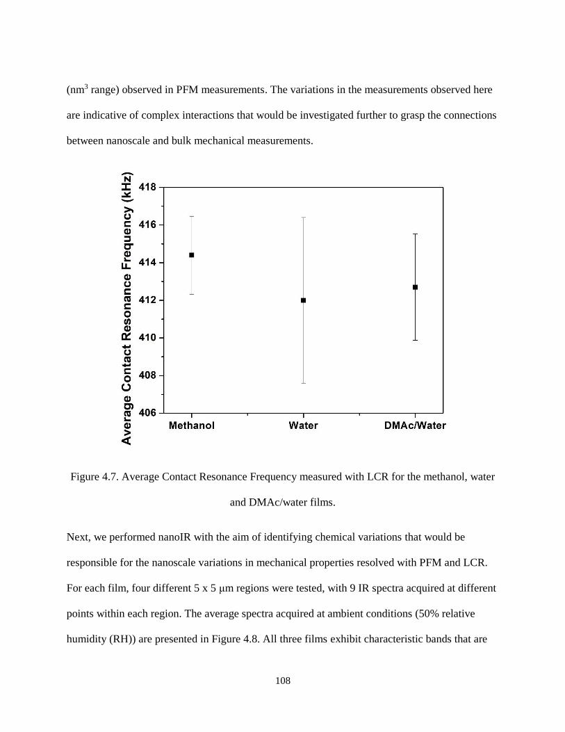
108

(nm3 range) observed in PFM measurements. The variations in the measurements observed here

are indicative of complex interactions that would be investigated further to grasp the connections

between nanoscale and bulk mechanical measurements.

Figure 4.7. Average Contact Resonance Frequency measured with LCR for the methanol, water

and DMAc/water films.

Next, we performed nanoIR with the aim of identifying chemical variations that would be

responsible for the nanoscale variations in mechanical properties resolved with PFM and LCR.

For each film, four different 5 x 5 μm regions were tested, with 9 IR spectra acquired at different

points within each region. The average spectra acquired at ambient conditions (50% relative

humidity (RH)) are presented in Figure 4.8. All three films exhibit characteristic bands that are

109

indicative of their composition. For instance, the bands observed at 1715-1730 cm-1 correspond

to C=O stretching in hemicellulose219, while the band at 1650 cm-1 corresponds to adsorbed OH

groups220. This band can also be attributed to ring-conjugated C=C in lignin. The band at 1715

cm-1 can also be attributed to unconjugated C=O groups in lignin220.

As it was difficult to resolve sharp IR bands under 50% RH, we repeated the measurements at

0% RH, obtained by purging the AFM chamber with nitrogen. The IR spectra show notable

differences in the individual bands for each film. For example, a band at 1560 cm-1, possibly

corresponding to lignin components233, has the lowest intensity in the methanol film, which is

not in agreement with the result obtained by Wang et al. in that DMAc/water film has the lowest

content of lignin and not the methanol film232. This is possibly due to the localized nature of this

measurement compared to the FTIR measurement used by Wang et al. Moreover, the band at

1650 cm-1 becomes narrower in all three films possibly due to removal of adsorbed OH groups

and being exclusively attributed to ring conjugated C=C in lignin at 0% RH.

With this configuration, we were able to measure the ratio of the intensity of the band at 1650

cm-1 to the intensity of the band at 1715-1730 cm-1. We found that it is highest in the

DMAc/Water film. Wang et al. found that DMAc/water film has the highest carbohydrate to

lignin ratio which might explain this variation. The band at 1650 cm-1 is most likely due to OH

groups adsorbed to the films. Overall, the nanoIR spectra obtained at 50% RH showed a broad

peak at 1650 cm-1 suggesting a high degree of adsorption of water molecules on all three films.

110

Figure 4.8. IR spectra obtained at 0% and 50% RH from (a) water film, (b) methanol film, and

(c) DMAc/water film. Blue curves indicate the measurements performed at ambient conditions

with 50% RH while red curves correspond to the measurements performed at low (close to 0%)

RH.

4.3 Example 2: Improving Yields of Tomato Plants Using Quantum Dots Coated with Growth

Promoters

Nanotechnology-enabled agriculture holds a promising future in one of three ways: internalizing

growth promoters and pesticides in an efficient and cost-effective manner, enhancing the ability

to detect crop diseases and conditions, and environmental stresses, and improving the plants

resistance to these external stresses18,234. In improving agricultural production, nanoparticles can

act as fertilizers by supplying the plants with nutrients directly, or acting as the vehicle to deliver

the nutrients in a more efficient way234,235. These nanoparticle-based fertilizers (or

“nanofertilizers”) offer several advantages including slow release of growth promoters as well as

more efficient nutrient uptake18. This minimizes the autrification and pollution caused by

excessive use of fertilizers, which can contaminate ground water with excess nitrogen for

decades236.

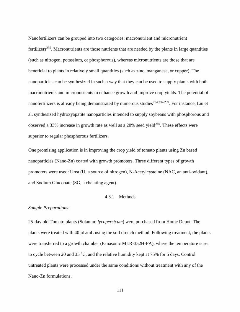
111

Nanofertilizers can be grouped into two categories: macronutrient and micronutrient

fertilizers235. Macronutrients are those nutrients that are needed by the plants in large quantities

(such as nitrogen, potassium, or phosphorous), whereas micronutrients are those that are

beneficial to plants in relatively small quantities (such as zinc, manganese, or copper). The

nanoparticles can be synthesized in such a way that they can be used to supply plants with both

macronutrients and micronutrients to enhance growth and improve crop yields. The potential of

nanofertilizers is already being demonstrated by numerous studies234,237-239. For instance, Liu et

al. synthesized hydroxyapatite nanoparticles intended to supply soybeans with phosphorous and

observed a 33% increase in growth rate as well as a 20% seed yield240. These effects were

superior to regular phosphorous fertilizers.

One promising application is in improving the crop yield of tomato plants using Zn based

nanoparticles (Nano-Zn) coated with growth promoters. Three different types of growth

promoters were used: Urea (U, a source of nitrogen), N-Acetylcysteine (NAC, an anti-oxidant),

and Sodium Gluconate (SG, a chelating agent).

4.3.1 Methods

Sample Preparations:

25-day old Tomato plants (Solanum lycopersicum) were purchased from Home Depot. The

plants were treated with 40 μL/mL using the soil drench method. Following treatment, the plants

were transferred to a growth chamber (Panasonic MLR-352H-PA), where the temperature is set

to cycle between 20 and 35 oC, and the relative humidity kept at 75% for 5 days. Control

untreated plants were processed under the same conditions without treatment with any of the

Nano-Zn formulations.

112

Confocal Raman Spectroscopy:

Confocal Raman spectroscopy measurements were performed using the WITec Alpha 300 RA

system with a 20X objective (Carl Zeiss EC EPIPLAN). Each of the Nano-Zn formulations was

tested by acquiring a 10 x 10 array of single spectra with an integration time of 1 s, and laser

power of ~ 5 mW. Raman mapping of the tomato plant stem tissues was acquired by recording a

single spectrum at 500 nm steps. A chemical map of the treatment distribution was then

constructed by calculating the intensity of the characteristic Raman band at 1040 cm-1.

Scanning Electron Microscopy:

SEM images were acquired using a Zeiss ULTRA-55 FEG system. The samples were coated

with gold-palladium prior to loading into the microscope’s vacuum chamber. InLens detector

was used with a working distance of 8 mm, a beam energy of 3 kV, and an electromagnetic lens

aperture of 20 μm.

4.3.2 Results

First, the Raman signature of each formulation was tested. Raman spectra of Nano-Zn coated

with SG exhibit a peak at 1040 cm-1 attributed to C-O stretching in SG (Figure 4.9 (b)). Raman

spectra of the plants confirmed the presence of the Nano-Zn coated with SG in stem cross

sections based on the presence of the strong band at 1040 cm-1. Furthermore, cube-like structures

were observed in SEM images acquired from Nano-Zn-SG treated tomato plants (Figure 4.9 (d)),

which could correspond to the effect of the Nano-Zn in the tissues, since the control experiment

did not show any such features. In addition, the data acquired for the other treatment did not

exhibit any such features.

113

Figure 4.9. (a) Optical image. (b) Raman spectra obtained from the stem cross section, bare

Nano-Zn, and SG coated Nano-Zn. (c) Raman map of the intensity of the band at 1040 cm-1

acquired from the region marked by the white square in (a). (d) SEM image of a stem cross

section of the tomato plant treated with SG coated Nano-Zn.

The effect of the Nano-Zn formulations on the physiological properties of the plants was also

considered (Figure 4.10), in collaboration with Dr. Santra and Dr. Das. The relative water

content (RWC) of the leaves was significantly enhanced in plants treated with all three coated

Nano-Zn formulations (Figure 4.10 (a)). RWC is important in that it shows how much water the

plants can retain under various conditions, and indicates that the Nano-Zn formulations can

improve the ability of the plants to withstand external stresses such as drought or salinity. The

114

membrane stability index (MSI) is used to measure the integrity of cell membranes. In this case,

the MSI values were higher for tomato plants treated with Nano-Zn formulations, indicating that

the cell membranes are more stable (Figure 4.10 (b)). Root and shoot lengths were also improved

in the Nano-Zn treated as compared to the untreated plants (Figures 4.10 (c) and (d)). The plants

treated with NAC coated Nano-Zn exhibited the largest average root and shoot lengths among

the three treatments. These results confirm the ability of Nano-Zn coated with growth promoters

115

to improve the yield of tomato plants, with strong implications for the future of using

nanoparticles as vehicles for the efficient delivery of growth promoters to plants.

Figure 4.10. Comparison of the Nano-Zn-Urea, Nano-Zn-NAC, and Nano-Zn-SG treated plants

with the control untreated plants. (a) Relative water content. (b) Membrane stability index. (c)

Root length, and (d) Shoot length. Figure adapted from the study performed by Dr. Smruti Das

[unpublished]241.

116

4.4 Summary

Two examples of adding value to agricultural production are discussed, with impacts on the food

energy water nexus. Biofuel production and biomass valorization, as well as enhancing crop

yields for improved food production constitute important activities, in which nanoscale

characterization has a major role to play. In the first example, the effect of using three different

coagulants on nanoscale properties of high performance carbon films prepared by deconstructing

hybrid poplar with autohydrolysis followed by ionic liquid pretreatment is studied. Nanoscale

chemical characterization using nanoIR reveals a change in the relative intensities of

characteristic peaks of the different films. However, our comparison to nanomechanical

measurements (LCR, PFM) suggest that nanoIR remains limited in characterizing materials with

high level of heterogeneity in their volume due to the large region excited by the IR laser focused

on the sample inducing interference in the photothermal measurements. Nanomechanical with

small volume displacement proved to be more sensitive to domains within the films of different

local stiffness.

In the second example, efficient delivery of growth promoters using Nano-Zn to young tomato

plants is demonstrated with positive effects on the plant physiology. Plants treated with all three

Nano-Zn formulations exhibited longer roots and shoots, as well as better water retention

capability and stronger membrane stability indexes. This shows that the treated plants can better

survive conditions such as droughts or high salinity. More importantly, it demonstrates how

nanoparticle based treatments can provide efficient delivery of growth promoters to plants,

avoiding overuse of fertilizers and/or pesticides which can pollute the environment and clean

water resources.

117

5 CONCLUSION

5.1 Overall Summary

In this dissertation, through various examples, the effects of mechanical and chemical stresses on

the structure and composition of plant cell walls were studied, as well as the potential of using

these phenomena to enhance energy and food production from the perspective of sustainable

agriculture. The work presented highlights the importance of realizing how food, energy, and

water security are interlinked in one nexus and their effects on each other must be considered in

any policies designed to promote each individual sector.

The effects of gravity on the structure and composition of plant cell walls were found to be

significant. Confocal Raman mapping combined with statistical analysis tools unveiled

variations in the characteristic signatures of cellulose and lignin between tension, opposite, and

normal wood. K-means clustering analysis made it possible to distinguish the different cell wall

layers based on the Raman spectra acquired in the area of the cell. Beyond that, our multi-

pronged approach facilitated a tailored selection of spectra from specific layers for further

analysis. The S/G ratio, a critical measure of the molecular structure of lignin, was confirmed to

be higher in tension wood than in normal wood. Cellulose crystallinity was measured for each

layer in tension and normal wood. The G layer was found to contain the most crystalline

cellulose microfibrils, as expected. However, we found that the middle lamella and S layer of

tension wood cell walls were more crystalline than their respective counterparts in opposite and

normal wood. Uncovering these subtle variations between tension wood and normal wood

constitutes a significant step in understanding how plants respond to external mechanical stress

at the cellular and subcellular levels.

118

Further, AFM based methods, namely AFAM and nanoIR, revealed variations within the cell

wall layers that could not be resolved by confocal Raman microscopy or standard AFM

topography mapping. AFAM phase mapping demonstrated local variation of 3° - 4° within 200

nm inside the S layer. These measurements were complemented with results from nanoIR to

label the composition of the features resolved in AFAM, although much remains to accomplish

to obtain a clear picture of molecular interaction in the plant cell wall.

The effects of chemical stresses in the form of treatments applied to citrus plants to combat citrus

greening disease could be studied using a multiscale approach. ZinkicideTM, a nanoparticle based

treatment designed to systemically enter the plant and directly target the pathogens, was

characterized using Raman spectroscopy and FTIR to identify the characteristic peaks, as well as

to monitor its stability over time. The Raman signature of the formulation allowed us to study the

uptake, translocation, and effects of ZinkicideTM on the plant through rapid screening of the

extracts. Treatment translocated inside the plant following 24 hours of root uptake was

identified. The distribution of Zn in the plant, though, required an elemental analysis. XRF and

EDS combined with SEM imaging were found to be complementary method to confirm the

uptake at the plant level but pinpoint the distribution of Zn in the vascular tissues such as phloem

and xylem. Using this approach, the ability of the treatment to reach the phloem and xylem

inside the leaves and stems of citrus plants was demonstrated. Overall, a robust protocol for

tracking the uptake of new nanoparticle-based treatments designed to combat plant disease was

developed and tested.

In addition to ZinkicideTM, a different Zn-based treatment for slow release through foliar

application, MS3T, was also studied using the aforementioned protocol. The characteristic

119

signature from the three individual components: clay, fixed quat and TSOL were obtained. As

the molecular structure of TSOL was unknown, our infrared spectroscopy studies combined with

molecular dynamics considerations (Dr. Loukas Petridis and his research group at the University

of Tennessee and Oak Ridge National Laboratory) allowed us to confirm that Zn forms a chelate

compound with urea by binding to the Oxygen atom in the carbonyl group. The foliar uptake of

the systemic active TSOL was demonstrated using elemental analysis techniques (EDS and

XRF) as well as FTIR combined with statistical analysis. It was shown that TSOL can penetrate

the leaves and translocate to the vascular system within 24 hours of foliar spray, with the

treatment deposited on the leaf surface for the duration of uptake. When combining TSOL with

clay for slower release, the measurements suggest that Zn penetrates the plants at a much slower

pace. These findings will be the subject of additional measurements in the near future. Our work

and the protocol developed is expected to have significant impact on the agricultural industry,

especially in supporting the design of new materials for tackling plant diseases and minimizing

their effects on the food sector of the food-energy-water nexus. Further quantitative and specific

monitoring of the treatment in the plant has the potential to support growers in adopting more

efficient use of treatments by determining appropriate field application times and optimizing

application frequency.

Lastly, we considered how tuning the properties of plants by application of external stresses

could be utilized to trigger plant responses towards obtaining new eco-friendly products, as well

as securing agricultural production efficiency. Valorization of biomass is sought after to improve

the financial competence of biorefineries rendering biofuel production as a more attractive

solution to the world’s impending energy crisis. One example of biomass products, namely

lignocellulosic-based films, was studied. The effect of varying one processing parameter, the

120

coagulating agent, on the nanoscale mechanical and chemical properties was monitored using

advanced AFM techniques. The stiffness and adhesion properties of the films were found to vary

greatly, with the film prepared using methanol being the least hydrophilic and the film prepared

using DMAc/water being the stiffest at the nanoscale. nanoIR measurements could not resolve

nanoscale chemical composition variations within a film at this time. However, the effect of

relative humidity on the films could be captured with nanoIR.

The last example focused on the effect of chemically induced stress from applying Nano-Zn

formulations coupled with growth promoters on tomato plants. Evidence of increased shoot and

root length in the treated plants could be reported, with the plants treated with Nano-Zn-NAC

showing the greatest variation. The water retention capability, as well as the cell membrane

integrity of the treated plants exhibited marked improvement compared to untreated plants.

These results show the promise of using nanoparticle treatments in combination with growth

promoting agents in enhancing the yields of important agricultural crops, which is of substantial

importance in the food-energy-water nexus and in meeting the demands on the 10 billion

population expected by 2050.

5.2 Future Directions

Our studies reveal interesting effects of mechanical and chemical stresses on the structure and

composition of plant cell walls, sometimes hidden in the building blocks – cellulose,

hemicellulose and lignin. However, the implications of these changes at the plant or population

level and what they mean remain partly unanswered. For instance the arrangement of these

biopolymers and their interactions is still not fully understood. With the advent of functional

nanoscale characterization tools and rigorous statistical analysis, fundamental behaviors of the

121

complex heterogeneous systems and their ultrastructure will likely become uncovered in the near

future. The long-term direction of this research involves designing new plant-derived materials,

based on the knowledge acquired of their structure and composition at the nanoscale, with more

favorable composition for the purpose of efficient biofuel extraction and added-value

bioproducts manufacturing which can compete on the market with synthetics.

Significant progress has been made in answering questions regarding the uptake and

translocation of key novel treatments in citrus plants to eradicate citrus greening disease. While it

was shown that the treatment can reach the phloem of the plants, it is still unknown in what form

the treatment exists inside the plant tissue. Are the nanoparticles still in their ZnO form? Or is the

Zn detected in elemental analysis simply Zn2+ ions? Different characterization methods such as

X-ray Photoelectron Spectroscopy (XPS) and cathodoluminescence may be able to provide the

answer. The mechanisms of entry in the plants also remain unclear. For instance, SEM images of

the treated surfaces showed aggregates of the MS3T treatment inside stomatal openings

suggesting that stomata could be gateways for the treatment to enter the leaves. However a lot of

unknowns remain.

Finally, the protocols developed in chapter 3 are already being used to study the uptake of

another copper-based treatment designed to tackle bacterial spot disease in tomato plants,

highlighting the strong potential of using these methods in studying novel chemical and

nanoparticle based treatments for plant diseases, and the potential broader impact this has on

food-energy-water nexus research.

Overall we expect that multiscale characterization and more particularly studies at the nanoscale

have an important role to play in meeting the demands of our growing world population.

122

APPENDIX A: BACKGROUND FOR RAMAN SPECTROSCOPY AND

IMAGING

123

Raman spectroscopy114,242 is one of two infrared methods that are the most commonly used for

plant research. In Raman scattering the incident light (generally in the visible range) distorts the

electron clouds around the nuclei in the molecule, causing transitions to excited virtual states. A

virtual state is short-lived before a photon is re-emitted as the electron transitions back to a lower

state. In cases where the electron cloud is only distorted with little or no influence on the motion

of the nuclei in the molecule, then the photon emitted presents little change in energy owing to

how light the electrons are compared to the nuclei. This rather small change in energy of the

scattered photons is called Rayleigh scattering.

When the interaction of the incident light with the molecules causes motion of the nuclei, Raman

inelastic scattering takes place and some of the photons emitted have different energy. This is a

weak process with the inelastically scattered intensity about 108 times weaker than Rayleigh

scattering. In the inelastic scattering process, energy can be exchanged between the molecule and

the light. In the case where light gains energy, it is termed anti-Stokes scattering, while in the

case where the molecule gains energy it is called Stokes scattering. Conventionally, this shift is

represented by the change in wavenumbers (cm-1) relative to the excitation wavelength. Figure

A.1 below shows the basic setup of Raman spectroscopy measurement.

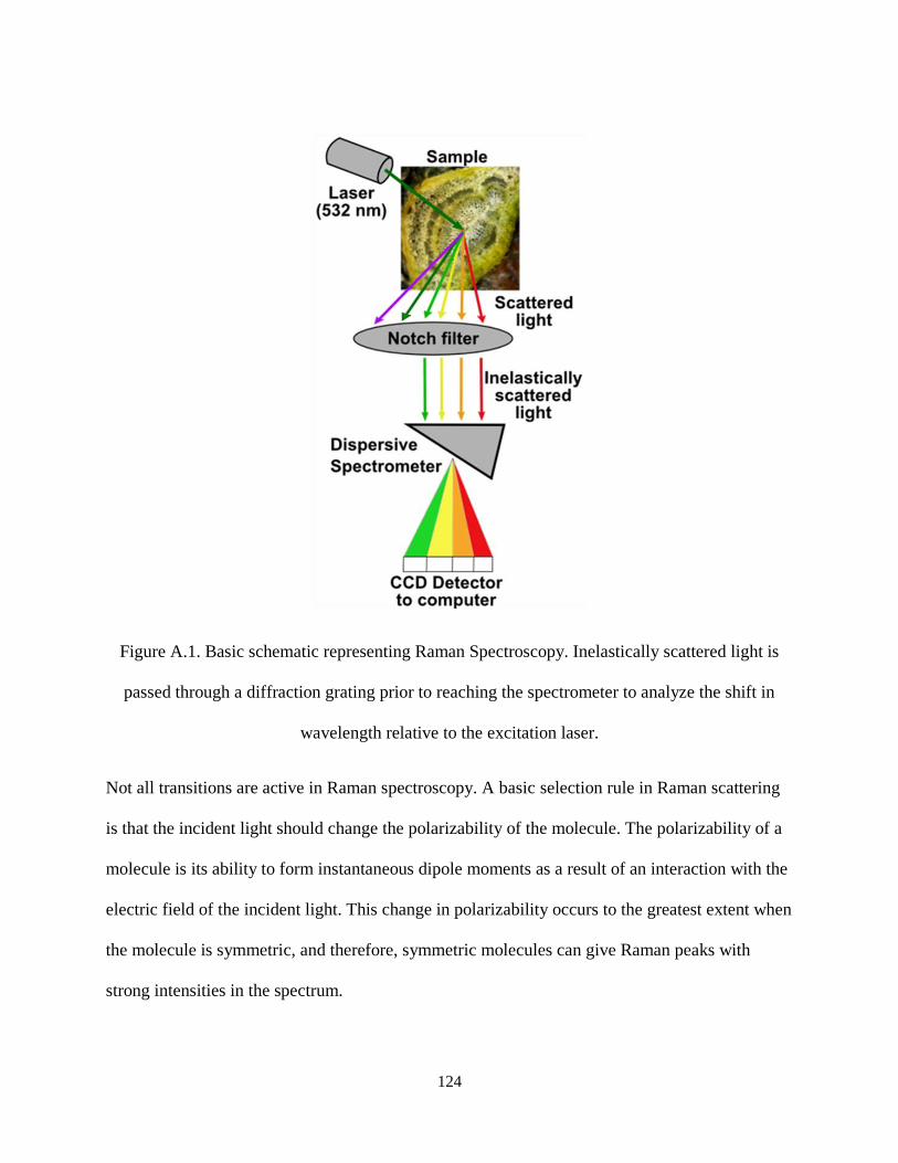
124

Figure A.1. Basic schematic representing Raman Spectroscopy. Inelastically scattered light is

passed through a diffraction grating prior to reaching the spectrometer to analyze the shift in

wavelength relative to the excitation laser.

Not all transitions are active in Raman spectroscopy. A basic selection rule in Raman scattering

is that the incident light should change the polarizability of the molecule. The polarizability of a

molecule is its ability to form instantaneous dipole moments as a result of an interaction with the

electric field of the incident light. This change in polarizability occurs to the greatest extent when

the molecule is symmetric, and therefore, symmetric molecules can give Raman peaks with

strong intensities in the spectrum.

125

Spatially resolved chemical information is a great interest in heterogeneous samples. It can be

obtained through IR or Raman imaging or mapping243. In imaging, the light is focused onto the

sample using appropriate lenses or objectives. Spectra are acquired for an array of points that

will become the “pixels” of the image. Raman mapping is usually more attractive than IR since

the wavelength of the excitation laser source in the visible range is almost 10 times smaller than

the mid-IR range, leading to much higher spatial resolution according to the diffraction limit

rule.

Confocal Raman microscopy242 is the most widely used method in chemical spectroscopic

imaging due to the combination of confocal microscopy principles with Raman scattering to

produce chemical images with resolutions down to around 250 nm. Modern systems also employ

CCD detectors, which can make the spectral acquisition faster, greatly reducing the time needed

to form the Raman map.

Although confocal Raman microscopy is advantageous in enabling faster acquisition of data,

there are still some issues that present an obstacle to characterization such as the limited spatial

resolution, the need to use higher integration times with samples which give lower intensity

Raman signals (since larger integration times reduce the signal-to-noise ratio), and the presence

of background fluorescence in many biological samples. Background fluorescence can be

overcome by using FTIR, and this is another way both characterization techniques are

complementary to each other.

126

APPENDIX B: BACKGROUND FOR FOURIER TRANSFORM

INFRARED SPECTROSCOPY

127

Fourier Transform Infrared Spectroscopy244 is the second type of infrared method commonly

used to study plant materials. In this case, the sample is illuminated with a broad range

illumination in the IR range. The detector is placed in the far field and records the spectrum to

identify the bands absorbed by the material.

When infrared light is used to illuminate a material, the photons are absorbed when their energy

matches the energy difference between the molecular vibrational states of the material following

a set of selection rules. The absorption spectrum gives information about which specific

frequencies of the infrared light (often expressed in wavenumber) are absorbed by the material.

Mid-IR spectroscopy focuses on the 4000-400 cm-1 range. Since no two materials have the same

set of absorption frequencies, an infrared spectrum is essentially a fingerprint of the material,

especially in the 1600-500 cm-1 region.

Originally infrared spectroscopy was carried out using “dispersive” methods which involved

shining the light at each frequency in the infrared range one at a time until a full spectrum was

obtained. Fourier Transform Infrared Spectroscopy (FTIR) was introduced to accelerate data

collection, by illuminating the sample with a broadband IR light: utilizing a Michelson

interferometer, an interferogram containing the information of the sample can be acquired. The

infrared spectrum is then obtained by taking the Fourier transform of the interferogram. Figure

B.1 shows an example of the basic setup of an FTIR spectrometer.

128

Figure B.1. Basic setup for FTIR245

Transmission techniques are the most popular ways to acquire FTIR spectra. The infrared beam

passes through the sample and is detected on the other side. Advantages of transmission spectra

include a high signal-to-noise ratio and the ability to scan a large variety of samples including

solids, liquids and gases. However, as with many transmission based characterization methods,

the “thickness” problem arises, and sample preparation for transmission based FTIRs is often

strenuous and time consuming. In many setups, Potassium Bromide (KBr) pellets, ZnS or ZnSe

plates, which are transparent to IR beams, are used as support and diluents for the samples.

Reflectance methods have the advantage of easier sample preparation but they also require an

expensive setup to align the beam and focus it on the sample, and collect it at the detector.

Another disadvantage of reflectance based FTIR is the small depth of penetration. Reflectance

based FTIR come in different varieties including: Diffuse Reflectance (DRIFTS) and Attenuated

Total Reflectance (ATR-FTIR). FTIR systems which use specular reflectance are also common.

DRIFTS is more suitable for solid and powdered samples, while ATR-FTIR is more suited for

films and liquids. ATR-FTIR requires the use of a crystal to achieve total internal reflection of

129

the IR beam, and form the evanescent wave that will interact with the sample. Figure B.2 shows

a schematic of how ATR-FTIR works.

Figure B.2. ATR-FTIR concept. The sample is placed on top of the crystal. An infrared beam is

passed through the crystal and undergoes total internal reflection with the surface in contact with

the sample. Evanescent waves from the beam are absorbed by the sample at the absorption

wavelengths before the beam reaches the detector.

The most commonly used crystal is Zinc Selenide (ZnSe); however, it can only acquire spectra

above 650 cm-1 which is a drawback for samples in which we are interested in observing

absorption bands lower than this range.

In contrast to Raman spectroscopy, in mid-IR spectroscopy stronger absorption occurs when

molecules have a larger change in their dipole moment. As such, the strongest peaks in an

infrared absorption spectrum often arise from asymmetric molecules.

Hence, Raman scattering and IR absorption are complementary spectroscopic techniques and

when used together can give a complete picture of a molecule’s vibrational modes and molecular

composition.

130

APPENDIX C: BACKGROUND FOR ATOMIC FORCE MICROSCOPY

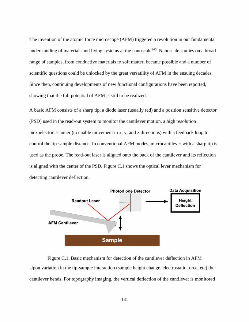
131

The invention of the atomic force microscope (AFM) triggered a revolution in our fundamental

understanding of materials and living systems at the nanoscale246. Nanoscale studies on a broad

range of samples, from conductive materials to soft matter, became possible and a number of

scientific questions could be unlocked by the great versatility of AFM in the ensuing decades.

Since then, continuing developments of new functional configurations have been reported,

showing that the full potential of AFM is still to be realized.

A basic AFM consists of a sharp tip, a diode laser (usually red) and a position sensitive detector

(PSD) used in the read-out system to monitor the cantilever motion, a high resolution

piezoelectric scanner (to enable movement in x, y, and z directions) with a feedback loop to

control the tip-sample distance. In conventional AFM modes, microcantilever with a sharp tip is

used as the probe. The read-out laser is aligned onto the back of the cantilever and its reflection

is aligned with the center of the PSD. Figure C.1 shows the optical lever mechanism for

detecting cantilever deflection.

Figure C.1. Basic mechanism for detection of the cantilever deflection in AFM

Upon variation in the tip-sample interaction (sample height change, electrostatic force, etc) the

cantilever bends. For topography imaging, the vertical deflection of the cantilever is monitored

132

as it scans the sample. The topography image is created by displaying the voltage read out by the

PSD at each point of the image and plotting the array in the 2D filled contour plot. However it is

possible to monitor other traits of the tip-sample interactions to map properties such as

mechanical, electrical, optical, thermal, and magnetic properties.

AFM microcantilevers shape, composition and tips should be selected with respect to the

imaging mode and the material to be imaged. In particular, the cantilever stiffness and/or natural

frequency, and its dimensions may play an important role in the quality of the images produced.

In general, longer cantilevers have lower stiffness and therefore can vibrate with larger

amplitudes during scanning. They are often preferred to image soft samples.

AFM imaging modes can be divided into two groups based on scanning dynamics: static and

dynamic modes. Static modes involve no driving in the cantilever, while dynamic modes involve

driving the cantilever at or near its resonance frequency.

Contact mode AFM is a static mode, in which the tip is engaged in contact with the sample. The

force between the tip and the sample is kept constant and may be used in the feedback loop.

Imaging is done in the repulsive regime of the interaction between the tip and the sample. The

deflection of the cantilever at each position in the scan is measured as previously described, and

gives topographic information on the sample. In addition to topographic information, friction

between the tip and the sample can also be measured by sensing the torsional movements of the

tip as it scans the sample. The force between the tip and the sample in contact mode AFM is

relatively high and in the range of 1 – 100 nN. This commonly causes damage in soft samples.

In tapping (or AC) mode, the cantilever is driven at or near its resonance frequency, and the

amplitude and phase of the cantilever vibrations change due to interactions with the sample. The

133

tip sample interaction forces are usually below 1 nN, which is advantageous for soft and

biological samples. In tapping mode AFM, the tip-sample distance is larger and the interactions

between the tip and the sample are governed by the attractive regime forces, such as vdW and

capillary forces. The small attractive interactions dampen the oscillations of the cantilever, and

give topographic information about the sample. In addition to topographic information, these

dynamic modes of AFM can be used to study long range interactions such as electrostatic and

magnetic forces.

Special consideration should be given to the force between the tip and the sample as it can reach

up to 1 nN and also cause damage to the sample. In general, the ratio of the amplitude setpoint

(defined by the user) and the amplitude of free oscillations is used to indicate the extent of

interactions between the tip and the sample.

In addition to topographic information, tapping mode phase imaging has been shown to provide

information about the stiffness of the sample as the phase shift in the cantilever oscillations is

strongly related to the sample stiffness and adhesion. However, for polymeric samples, other

factors can influence this kind of measurement such as the polymer’s viscoelastic response,

capillary forces, and changes in the contact area, which is a critical factor in determining the

stiffness of a material.

The power of AFM lies in its ability to scan samples under different environmental conditions

with minimal sample preparation (as compared to characterization methods such as Scanning and

Transmission Electron Microscopies), and achieve high resolution, with atomic scale resolution

attainable under specific conditions.

134

APPENDIX D: COPYRIGHT PERMISSION FOR FIGURE 2.16

135

136

APPENDIX E: COPYRIGHT PERMISSIONS FOR FIGURE 3.1

137

Copyright Permission for Figure 3.1 (a)

Copyright Permission for Figure 3.1 (b)

138

APPENDIX F: COPYRIGHT PERMISSION FOR FIGURE 4.1

139

140

LIST OF REFERENCES

1 IEA. World Energy Outlook 2017. (Organisation for Economic Co-operation and

Development, OECD, 2017).

2 Elbehri, A. et al. FAO-IPCC Expert Meeting on Climate Change, Land Use and Food

Security: Final Meeting Report. Rome: FAO and IPCC, (2017).

3 Bakker, K. Water security: research challenges and opportunities. Science 337, 914-915,

(2012).

4 Turral, H., Burke, J. J. & Faurès, J.-M. Climate change, water and food security. (Food

and Agriculture Organization of the United Nations Rome, Italy, 2011).

5 Godfray, H. C. J. et al. Food Security: The Challenge of Feeding 9 Billion People.

Science 327, 812, (2010).

6 Rasul, G. & Sharma, B. The nexus approach to water–energy–food security: an option for

adaptation to climate change. Climate Policy 16, 682-702, (2016).

7 Biggs, E. M. et al. Sustainable development and the water–energy–food nexus: A

perspective on livelihoods. Environmental Science & Policy 54, 389-397, (2015).

8 Fereres, E. & Soriano, M. A. Deficit irrigation for reducing agricultural water use.

Journal of experimental botany 58, 147-159, (2006).

9 Belder, P. et al. Effect of water-saving irrigation on rice yield and water use in typical

lowland conditions in Asia. Agricultural Water Management 65, 193-210, (2004).

10 Kang, S. et al. Effects of limited irrigation on yield and water use efficiency of winter

wheat in the Loess Plateau of China. Agricultural water management 55, 203-216,

(2002).

141

11 Rathmann, R., Szklo, A. & Schaeffer, R. Land use competition for production of food

and liquid biofuels: An analysis of the arguments in the current debate. Renewable

Energy 35, 14-22, (2010).

12 Leck, H., Conway, D., Bradshaw, M. & Rees, J. Tracing the Water–Energy–Food Nexus:

Description, Theory and Practice. Geography Compass 9, 445-460, (2015).

13 Beddington, J. in Lecture to Sustainable Development UK 09 Conference.

14 Endo, A., Tsurita, I., Burnett, K. & Orencio, P. M. A review of the current state of

research on the water, energy, and food nexus. Journal of Hydrology: Regional Studies

11, 20-30, (2017).

15 Prasad, R., Bhattacharyya, A. & Nguyen, Q. D. Nanotechnology in Sustainable

Agriculture: Recent Developments, Challenges, and Perspectives. Frontiers in

Microbiology 8, (2017).

16 Servin, A. et al. A review of the use of engineered nanomaterials to suppress plant

disease and enhance crop yield. Journal of Nanoparticle Research 17, 1-21, (2015).

17 Parisi, C., Vigani, M. & Rodríguez-Cerezo, E. Agricultural Nanotechnologies: What are

the current possibilities? Nano Today 10, 124-127, (2015).

18 Sekhon, B. S. Nanotechnology in agri-food production: an overview. Nanotechnology,

Science and Applications 7, 31-53, (2014).

19 Menéndez-Manjón, A., Moldenhauer, K., Wagener, P. & Barcikowski, S. Nano-energy

research trends: bibliometrical analysis of nanotechnology research in the energy sector.

Journal of Nanoparticle Research 13, 3911-3922, (2011).

20 Serrano, E., Rus, G. & Garcia-Martinez, J. Nanotechnology for sustainable energy.

Renewable and Sustainable Energy Reviews 13, 2373-2384, (2009).

142

21 Brame, J., Li, Q. & Alvarez, P. J. Nanotechnology-enabled water treatment and reuse:

emerging opportunities and challenges for developing countries. Trends in Food Science

& Technology 22, 618-624, (2011).

22 Savage, N. & Diallo, M. S. Nanomaterials and water purification: opportunities and

challenges. Journal of Nanoparticle research 7, 331-342, (2005).

23 Li, Y.-H. et al. Competitive adsorption of Pb2+, Cu2+ and Cd2+ ions from aqueous

solutions by multiwalled carbon nanotubes. Carbon 41, 2787-2792, (2003).

24 Ji, L., Lin, Z., Alcoutlabi, M. & Zhang, X. Recent developments in nanostructured anode

materials for rechargeable lithium-ion batteries. Energy & Environmental Science 4,

2682-2699, (2011).

25 Huang, H., Yin, S. C., Kerr, T., Taylor, N. & Nazar, L. F. Nanostructured composites: a

high capacity, fast rate Li3V2 (PO4) 3/carbon cathode for rechargeable lithium batteries.

Advanced Materials 14, 1525-1528, (2002).

26 Elkin, T. et al. Immuno‐Carbon Nanotubes and Recognition of Pathogens.

ChemBioChem 6, 640-643, (2005).

27 Hughes, L. The four ‘R's of energy security. Energy Policy 37, 2459-2461, (2009).

28 Winzer, C. Conceptualizing energy security. Energy policy 46, 36-48, (2012).

29 Petroleum, B. BP statistical review of world energy. (London: British Petroleum, 2017).

30 Höök, M. & Tang, X. Depletion of fossil fuels and anthropogenic climate change—A

review. Energy Policy 52, 797-809, (2013).

31 Harrington, W. Fuel economy and motor vehicle emissions. Journal of environmental

economics and management 33, 240-252, (1997).

143

32 Baetens, R., Jelle, B. P. & Gustavsen, A. Aerogel insulation for building applications: a

state-of-the-art review. Energy and Buildings 43, 761-769, (2011).

33 Baetens, R. et al. Vacuum insulation panels for building applications: A review and

beyond. Energy and Buildings 42, 147-172, (2010).

34 Nardelli, A., Deuschle, E., de Azevedo, L. D., Pessoa, J. L. N. & Ghisi, E. Assessment of

Light Emitting Diodes technology for general lighting: A critical review. Renewable and

Sustainable Energy Reviews 75, 368-379, (2017).

35 Jacobson, M. Z. Review of solutions to global warming, air pollution, and energy

security. Energy & Environmental Science 2, 148-173, (2009).

36 Sawin, J. L. et al. Renewables 2017 Global Status Report. (2013).

37 Singh, G. K. Solar power generation by PV (photovoltaic) technology: A review. Energy

53, 1-13, (2013).

38 Solangi, K., Islam, M., Saidur, R., Rahim, N. & Fayaz, H. A review on global solar

energy policy. Renewable and sustainable energy reviews 15, 2149-2163, (2011).

39 Islam, M., Mekhilef, S. & Saidur, R. Progress and recent trends of wind energy

technology. Renewable and Sustainable Energy Reviews 21, 456-468, (2013).

40 Westwood, A. Ocean power: Wave and tidal energy review. Refocus 5, 50-55, (2004).

41 Yue, D., You, F. & Snyder, S. W. Biomass-to-bioenergy and biofuel supply chain

optimization: Overview, key issues and challenges. Computers & Chemical Engineering

66, 36-56, (2014).

42 Solomon, B. D. Biofuels and sustainability. Annals of the New York Academy of Sciences

1185, 119-134, (2010).

144

43 Tilman, D. et al. Beneficial Biofuels—The Food, Energy, and Environment Trilemma.

Science 325, 270, (2009).

44 Lund, J. W., Freeston, D. H. & Boyd, T. L. Direct utilization of geothermal energy 2010

worldwide review. Geothermics 40, 159-180, (2011).

45 Yüksel, I. Development of hydropower: a case study in developing countries. Energy

Sources, Part B 2, 113-121, (2007).

46 Malézieux, E. et al. in Sustainable agriculture 329-353 (Springer, 2009).

47 Reinhardt, E. D., Keane, R. E., Calkin, D. E. & Cohen, J. D. Objectives and

considerations for wildland fuel treatment in forested ecosystems of the interior western

United States. Forest Ecology and Management 256, 1997-2006, (2008).

48 Solomon, B. & Luzadis, V. A. Renewable energy from forest resources in the United

States. (Routledge, 2008).

49 Bothast, R. & Schlicher, M. Biotechnological processes for conversion of corn into

ethanol. Applied microbiology and biotechnology 67, 19-25, (2005).

50 Sun, Y. & Cheng, J. Hydrolysis of lignocellulosic materials for ethanol production: a

review. Bioresource Technology 83, 1-11, (2002).

51 Field, C. B., Campbell, J. E. & Lobell, D. B. Biomass energy: the scale of the potential

resource. Trends in Ecology & Evolution 23, 65-72, (2008).

52 Zhao, X., Zhang, L. & Liu, D. Biomass recalcitrance. Part I: the chemical compositions

and physical structures affecting the enzymatic hydrolysis of lignocellulose. Biofuels,

Bioproducts and Biorefining 6, 465-482, (2012).

145

53 Zhao, X., Zhang, L. & Liu, D. Biomass recalcitrance. Part II: Fundamentals of different

pre-treatments to increase the enzymatic digestibility of lignocellulose. Biofuels,

Bioproducts and Biorefining 6, 561-579, (2012).

54 Albersheim, P., Darvill, A., Roberts, K., Sederoff, R. & Staehelin, A. Plant Cell Walls.

67-95 (Garland Science, 2011).

55 Himmel, M. E. Biomass recalcitrance: deconstructing the plant cell wall for bioenergy.

(Wiley Online Library, 2008).

56 Himmel, M. E. et al. Biomass recalcitrance: engineering plants and enzymes for biofuels

production. science 315, 804-807, (2007).

57 Pinstrup-Andersen, P. Food security: definition and measurement. Food Security 1, 5-7,

(2009).

58 Ericksen, P. J., Ingram, J. S. I. & Liverman, D. M. Food security and global

environmental change: emerging challenges. Environmental Science & Policy 12, 373-

377, (2009).

59 Wheeler, T. & Von Braun, J. Climate change impacts on global food security. Science

341, 508-513, (2013).

60 Knox, J., Hess, T., Daccache, A. & Wheeler, T. Climate change impacts on crop

productivity in Africa and South Asia. Environmental Research Letters 7, 034032,

(2012).

61 Mansfield, J. et al. Top 10 plant pathogenic bacteria in molecular plant pathology.

Molecular Plant Pathology 13, 614-629, (2012).

62 Strange, R. N. & Scott, P. R. Plant Disease: A Threat to Global Food Security. Annual

Review of Phytopathology 43, 83-116, (2005).

146

63 Scurfield, G. Reaction Wood: Its Structure and Function. Lignification may generate the

force active in restoring the trunks of leaning trees to the vertical 179, 647-655, (1973).

64 Anten, N. P., Casado-Garcia, R. & Nagashima, H. Effects of mechanical stress and plant

density on mechanical characteristics, growth, and lifetime reproduction of tobacco

plants. The American Naturalist 166, 650-660, (2005).

65 Biddington, N. L. & Dearman, A. S. The Effect of Mechanically Induced Stress on the

Growth of Cauliflower, Lettuce and Celery Seedlings. Annals of Botany 55, 109-119,

(1985).

66 Jaffe, M. J. Morphogenetic Responses of Plants to Mechanical Stimuli or Stress.

BioScience 30, 239-243, (1980).

67 Tuck, C. O., Pérez, E., Horváth, I. T., Sheldon, R. A. & Poliakoff, M. Valorization of

Biomass: Deriving More Value from Waste. Science 337, 695, (2012).

68 Biddington, N. L. The effects of mechanically-induced stress in plants — a review. Plant

Growth Regulation 4, 103-123, (1986).

69 Lintilhac, P. M. & Vesecky, T. B. Mechanical Stress and Cell Wall Orientation in Plants.

II. The Application of Controlled Directional Stress to Growing Plants; with a Discussion

on the Nature of the Wound Reaction. American Journal of Botany 68, 1222-1230,

(1981).

70 Takahashi, H. & Suge, H. Sex expression in cucumber plants as affected by mechanical

stress. Plant and cell physiology 21, 303-310, (1980).

71 Telewski, F. W. Is windswept tree growth negative thigmotropism? Plant science 184,

20-28, (2012).

147

72 Blancaflor, E. B. & Masson, P. H. Plant gravitropism. Unraveling the ups and downs of a

complex process. Plant Physiology 133, 1677-1690, (2003).

73 Monshausen, G. B., Swanson, S. J. & Gilroy, S. Touch sensing and thigmotropism. Plant

Tropisms. Blackwell, Ames, IA, 91-122, (2008).

74 Braam, J. In touch: plant responses to mechanical stimuli. New Phytologist 165, 373-389,

(2005).

75 Pressman, E., Huberman, M., Aloni, B. & Jaffe, M. J. Thigmomorphogenesis: the Effect

of Mechanical Perturbation and Ethrel on Stem Pithiness in Tomato [Lycopersicon

esculentum (Mill.) Plants]. Annals of Botany 52, 93-100, (1983).

76 Jaffe, M. J. Thigmomorphogenesis: The response of plant growth and development to

mechanical stimulation. Planta 114, 143-157, (1973).

77 Beardsell, M. Effects of routine handling on maize growth. Functional Plant Biology 4,

857-861, (1977).

78 Shawish, O. & Baker, R. Thigmomorphogenesis and Predisposition of Hosts to Fusarium

Wilt. Phytopathology 72, 63-68, (1982).

79 Suge, H. Dehydration and drought resistance in Phaseolus vulgaris as affected by

mechanical stress. Reports of the Institute for Agricultural Research, Tohoku University

31, 1-10, (1980).

80 Sannigrahi, P., Ragauskas, A. J. & Tuskan, G. A. Poplar as a feedstock for biofuels: A

review of compositional characteristics. Biofuels, Bioproducts and Biorefining 4, 209-

226, (2010).

81 Norberg Per, H. & Meier, H. in Holzforschung - International Journal of the Biology,

Chemistry, Physics and Technology of Wood Vol. 20 174 (1966).

148

82 Daniel, G., Filonova, L., Kallas Åsa, M. & Teeri Tuula, T. in Holzforschung Vol. 60

618 (2006).

83 Hedenström, M. et al. Identification of Lignin and Polysaccharide Modifications in

Populus Wood by Chemometric Analysis of 2D NMR Spectra from Dissolved Cell

Walls. Molecular Plant 2, 933-942, (2009).

84 Foston, M. et al. Chemical, ultrastructural and supramolecular analysis of tension wood

in Populus tremula x alba as a model substrate for reduced recalcitrance. Energy &

Environmental Science 4, 4962-4971, (2011).

85 Sawada, D. et al. Tension wood structure and morphology conducive for better

enzymatic digestion. Biotechnology for Biofuels 11, 44, (2018).

86 Wada, M., Okano, T., Sugiyama, J. & Horii, F. Characterization of tension and normally

lignified wood cellulose inPopulus maximowiczii. Cellulose 2, 223-233, (1995).

87 Al-Haddad, J. M., Kang, K.-Y., Mansfield, S. D. & Telewski, F. W. Chemical responses

to modified lignin composition in tension wood of hybrid poplar (Populus

tremula × Populus alba). Tree Physiology 33, 365-373, (2013).

88 Sun, L. et al. Rapid determination of syringyl: Guaiacyl ratios using FT-Raman

spectroscopy. Biotechnology and Bioengineering 109, 647-656, (2012).

89 Stewart, D. Lignin as a base material for materials applications: Chemistry, application

and economics. Industrial Crops and Products 27, 202-207, (2008).

90 Zhang, L., Xu, C. C. & Champagne, P. Overview of recent advances in thermo-chemical

conversion of biomass. Energy Conversion and Management 51, 969-982, (2010).

149

91 Goyal, H., Seal, D. & Saxena, R. Bio-fuels from thermochemical conversion of

renewable resources: a review. Renewable and sustainable energy reviews 12, 504-517,

(2008).

92 Gierlinger, N. & Schwanninger, M. Chemical Imaging of Poplar Wood Cell Walls by

Confocal Raman Microscopy. Plant Physiology 140, 1246-1254, (2006).

93 Gierlinger, N. & Schwanninger, M. The potential of Raman microscopy and Raman

imaging in plant research. Spectroscopy 21, 69-89, (2007).

94 Zhang, X. et al. Method for Automatically Identifying Spectra of Different Wood Cell

Wall Layers in Raman Imaging Data Set. Analytical Chemistry 87, 1344-1350, (2015).

95 Gierlinger, N., Keplinger, T. & Harrington, M. Imaging of plant cell walls by confocal

Raman microscopy. Nat. Protocols 7, 1694-1708, (2012).

96 Gierlinger, N. et al. Cellulose microfibril orientation of Picea abies and its variability at

the micron-level determined by Raman imaging. Journal of Experimental Botany 61,

587-595, (2010).

97 Agarwal, U. P. Raman imaging to investigate ultrastructure and composition of plant cell

walls: distribution of lignin and cellulose in black spruce wood (Picea mariana). Planta

224, 1141-1153, (2006).

98 Gierlinger, N., Keplinger, T., Harrington, M. & Schwanninger, M. in Cellulose - Biomass

Conversion (eds Theo van de Ven & John Kadla) Ch. 08 (InTech, 2013).

99 Agarwal, U. P., Reiner, R. S. & Ralph, S. A. Cellulose I crystallinity determination using

FT–Raman spectroscopy: univariate and multivariate methods. Cellulose 17, 721-733,

(2010).

150

100 Agarwal, U. P., Reiner, R. R. & Ralph, S. A. Estimation of Cellulose Crystallinity of

Lignocelluloses Using Near-IR FT-Raman Spectroscopy and Comparison of the Raman

and Segal-WAXS Methods. Journal of Agricultural and Food Chemistry 61, 103-113,

(2013).

101 Fischer, S., Schenzel, K., Fischer, K. & Diepenbrock, W. Applications of FT Raman

Spectroscopy and Micro Spectroscopy Characterizing Cellulose and Cellulosic

Biomaterials. Macromolecular Symposia 223, 41-56, (2005).

102 TetardL, PassianA, Farahi, R. H., ThundatT & Davison, B. H. Opto-nanomechanical

spectroscopic material characterization. Nat Nano 10, 870-877, (2015).

103 Kirby, A. R., Gunning, A. P., Waldron, K. W., Morris, V. J. & Ng, A. Visualization of

plant cell walls by atomic force microscopy. Biophysical Journal 70, 1138-1143, (1996).

104 Davies, L. M. & Harris, P. J. Atomic force microscopy of microfibrils in primary cell

walls. Planta 217, 283-289, (2003).

105 Milani, P. et al. In vivo analysis of local wall stiffness at the shoot apical meristem in

Arabidopsis using atomic force microscopy. The Plant Journal 67, 1116-1123, (2011).

106 Carr, S. & Carr, D. Intercellular pectic strands in parenchyma: studies of plant cell walls

by scanning electron microscopy. Australian Journal of Botany 23, 95-105, (1975).

107 Tetard, L., Passian, A., Jung, S., Ragauskas, A. J. & Davison, B. H. Development of new

methods in scanning probe microscopy for lignocellulosic biomass characterization.

Industrial Biotechnology 8, 245-249, (2012).

108 Farahi, R. H. et al. Plasticity, elasticity, and adhesion energy of plant cell walls:

nanometrology of lignin loss using atomic force microscopy. Scientific Reports 7, 152,

(2017).

151

109 Muraille, L., Aguié-Béghin, V., Chabbert, B. & Molinari, M. Bioinspired lignocellulosic

films to understand the mechanical properties of lignified plant cell walls at nanoscale. 7,

44065, (2017).

110 Yamanaka, K., Ogiso, H. & Kolosov, O. Ultrasonic force microscopy for nanometer

resolution subsurface imaging. Applied Physics Letters 64, 178-180, (1994).

111 Rabe, U. & Arnold, W. Acoustic microscopy by atomic force microscopy. Applied

Physics Letters 64, 1493-1495, (1994).

112 Dazzi, A. & Prater, C. B. AFM-IR: Technology and Applications in Nanoscale Infrared

Spectroscopy and Chemical Imaging. Chemical Reviews 117, 5146-5173, (2017).

113 Jung, S., Foston, M., Sullards, M. C. & Ragauskas, A. J. Surface Characterization of

Dilute Acid Pretreated Populus deltoides by ToF-SIMS. Energy & Fuels 24, 1347-1357,

(2010).

114 Hollricher, O. in Confocal Raman Microscopy (eds Thomas Dieing, Olaf Hollricher, &

Jan Toporski) 43-60 (Springer Berlin Heidelberg, 2011).

115 Žalik, K. R. An efficient k′-means clustering algorithm. Pattern Recognition Letters 29,

1385-1391, (2008).

116 MacQueen, J. in Proc. 5th Berkeley Symposium on Mathematical Statistics and

Probability, 1967. 281-297.

117 Wold, S., Esbensen, K. & Geladi, P. Principal component analysis. Chemometrics and

intelligent laboratory systems 2, 37-52, (1987).

118 Jolliffe, I. T. in Principal component analysis 115-128 (Springer, 1986).

152

119 Park, S., Baker, J. O., Himmel, M. E., Parilla, P. A. & Johnson, D. K. Cellulose

crystallinity index: measurement techniques and their impact on interpreting cellulase

performance. Biotechnology for Biofuels 3, 1-10, (2010).

120 Zhang, X., Chen, S., Ramaswamy, S., Kim, Y. S. & Xu, F. Obtaining pure spectra of

hemicellulose and cellulose from poplar cell wall Raman imaging data. Cellulose, (2017).

121 Agarwal, U. P. & Ralph, S. A. FT-Raman Spectroscopy of Wood: Identifying

Contributions of Lignin and Carbohydrate Polymers in the Spectrum of Black Spruce

(Picea mariana). Appl. Spectrosc. 51, 1648-1655, (1997).

122 Barsberg, S., Matousek, P., Towrie, M., Jørgensen, H. & Felby, C. Lignin Radicals in the

Plant Cell Wall Probed by Kerr-Gated Resonance Raman Spectroscopy. Biophysical

Journal 90, 2978-2986, (2006).

123 Saariaho, A.-M., Jääskeläinen, A.-S., Nuopponen, M. & Vuorinen, T. Ultra Violet

Resonance Raman Spectroscopy in Lignin Analysis: Determination of Characteristic

Vibrations of p-Hydroxyphenyl, Guaiacyl, and Syringyl Lignin Structures. Appl.

Spectrosc. 57, 58-66, (2003).

124 Larsen, K. L. & Barsberg, S. Theoretical and Raman Spectroscopic Studies of Phenolic

Lignin Model Monomers. The Journal of Physical Chemistry B 114, 8009-8021, (2010).

125 Nishikubo, N. et al. Xyloglucan Endo-transglycosylase (XET) Functions in Gelatinous

Layers of Tension Wood Fibers in Poplar—A Glimpse into the Mechanism of the

Balancing Act of Trees. Plant and Cell Physiology 48, 843-855, (2007).

126 Schenzel, K., Fischer, S. & Brendler, E. New method for determining the degree of

cellulose I crystallinity by means of FT Raman spectroscopy. Cellulose 12, (2005).

153

127 Eichhorn, S., Hughes, M., Snell, R. & Mott, L. Strain induced shifts in the Raman spectra

of natural cellulose fibers. Journal of materials science letters 19, 721-723, (2000).

128 Gierlinger, N., Schwanninger, M., Reinecke, A. & Burgert, I. Molecular changes during

tensile deformation of single wood fibers followed by Raman microscopy.

Biomacromolecules 7, 2077-2081, (2006).

129 Soliman, M. & Tetard, L. Probing Chemical and Physical Properties of Poplar Tension

Wood Using Confocal Raman Microscopy and Pulsed Force Mode Atomic Force

Microscopy. MRS Advances 2, 1103-1109, (2017).

130 Hu, S., Su, C. & Arnold, W. Imaging of subsurface structures using atomic force acoustic

microscopy at GHz frequencies. Journal of Applied Physics 109, 084324, (2011).

131 Striegler, A. et al. Detection of buried reference structures by use of atomic force

acoustic microscopy. Ultramicroscopy 111, 1405-1416, (2011).

132 Cunfu, H., Gaimei, Z., Bin, W. & Zaiqi, W. Subsurface defect of the SiOx film imaged

by atomic force acoustic microscopy. Optics and Lasers in Engineering 48, 1108-1112,

(2010).

133 Stan, G. & Solares, S. D. Frequency, amplitude, and phase measurements in contact

resonance atomic force microscopies. Beilstein journal of nanotechnology 5, 278, (2014).

134 Sofla, M. R. K., Brown, R. J., Tsuzuki, T. & Rainey, T. J. A comparison of cellulose

nanocrystals and cellulose nanofibres extracted from bagasse using acid and ball milling

methods. Advances in Natural Sciences: Nanoscience and Nanotechnology 7, 035004,

(2016).

135 Mandal, A. & Chakrabarty, D. Isolation of nanocellulose from waste sugarcane bagasse

(SCB) and its characterization. Carbohydrate Polymers 86, 1291-1299, (2011).

154

136 Kole, C. et al. Nanobiotechnology can boost crop production and quality: first evidence

from increased plant biomass, fruit yield and phytomedicine content in bitter melon

(Momordica charantia). BMC Biotechnology 13, 37, (2013).

137 Rico, C. M. et al. Cerium Oxide Nanoparticles Impact Yield and Modify Nutritional

Parameters in Wheat (Triticum aestivum L.). Journal of Agricultural and Food

Chemistry 62, 9669-9675, (2014).

138 Tripathi, D. K. et al. An overview on manufactured nanoparticles in plants: Uptake,

translocation, accumulation and phytotoxicity. Plant Physiology and Biochemistry 110,

2-12, (2017).

139 Ma, X., Geiser-Lee, J., Deng, Y. & Kolmakov, A. Interactions between engineered

nanoparticles (ENPs) and plants: Phytotoxicity, uptake and accumulation. Science of The

Total Environment 408, 3053-3061, (2010).

140 Lichtfouse, E. et al. in Sustainable Agriculture (eds Eric Lichtfouse et al.) 1-7 (Springer

Netherlands, 2009).

141 Lal, R. in Sustainable Agriculture (eds Eric Lichtfouse et al.) 15-23 (Springer

Netherlands, 2009).

142 Condon, A. G., Richards, R. A., Rebetzke, G. J. & Farquhar, G. D. Improving Intrinsic

Water-Use Efficiency and Crop Yield. Crop Science 42, 122-131, (2002).

143 Fageria, N. K. The Use of Nutrients in Crop Plants. 1st Edition edn, (Taylor & Francis,

2008).

144 Aktar, M. W., Sengupta, D. & Chowdhury, A. Impact of pesticides use in agriculture:

their benefits and hazards. Interdisciplinary Toxicology 2, 1-12, (2009).

155

145 Hippler, F. W. R. et al. Uptake and Distribution of Soil Applied Zinc by Citrus Trees—

Addressing Fertilizer Use Efficiency with 68Zn Labeling. PLOS ONE 10, e0116903,

(2015).

146 Fernández, V. & Brown, P. H. From plant surface to plant metabolism: the uncertain fate

of foliar-applied nutrients. Frontiers in Plant Science 4, 289, (2013).

147 Gooding, M. J. & Davies, W. P. Foliar urea fertilization of cereals: A review. Fertilizer

research 32, 209-222, (1992).

148 Fageria, N. K., Filho, M. P. B., Moreira, A. & Guimarães, C. M. Foliar Fertilization of

Crop Plants. Journal of Plant Nutrition 32, 1044-1064, (2009).

149 Fernández, V. & Ebert, G. Foliar iron fertilization: a critical review. Journal of plant

nutrition 28, 2113-2124, (2005).

150 Tans-Kersten, J., Huang, H. & Allen, C. Ralstonia solanacearum needs motility for

invasive virulence on tomato. Journal of bacteriology 183, 3597-3605, (2001).

151 Buell, C. R. et al. The complete genome sequence of the Arabidopsis and tomato

pathogen Pseudomonas syringae pv. tomato DC3000. Proceedings of the National

Academy of Sciences 100, 10181-10186, (2003).

152 Elphinstone, J., Stanford, H. & Stead, D. in Bacterial Wilt Disease 133-139 (Springer,

1998).

153 Zhang, Z., Coyne, D. P., Vidaver, A. K. & Mitra, A. Expression of human lactoferrin

cDNA confers resistance to Ralstonia solanacearum in transgenic tobacco plants.

Phytopathology 88, 730-734, (1998).

156

154 Thilmony, R. L., Chen, Z., Bressan, R. A. & Martin, G. B. Expression of the tomato Pto

gene in tobacco enhances resistance to Pseudomonas syringae pv tabaci expressing

avrPto. The Plant Cell 7, 1529-1536, (1995).

155 Bendix, C. & Lewis, J. D. The enemy within: phloem-limited pathogens. Molecular Plant

Pathology, n/a-n/a, (2017).

156 Bae, C. et al. Infection processes of xylem-colonizing pathogenic bacteria: possible

explanations for the scarcity of qualitative disease resistance genes against them in crops.

Theoretical and Applied Genetics 128, 1219-1229, (2015).

157 Bové, J. M. & Garnier, M. Phloem-and xylem-restricted plant pathogenic bacteria. Plant

Science 164, 423-438, (2003).

158 da Graça, J. V. et al. Huanglongbing: An overview of a complex pathosystem ravaging

the world's citrus. Journal of Integrative Plant Biology 58, 373-387, (2016).

159 Texeira, D. C. et al. First Report of a Huanglongbing-Like Disease of Citrus in Sao Paulo

State, Brazil and Association of a New Liberibacter Species, “Candidatus Liberibacter

americanus”, with the Disease. Plant Disease 89, 107-107, (2005).

160 Guo, Y., Woods, P. & Rooney-Latham, S. First report of Candidatus Liberibacter

asiaticus associated with citrus huanglongbing in California. Current Microbiology 69,

554-560, (2014).

161 da Graça, J. et al. Huanglongbing in Texas: Report on the first detections in commercial

citrus. Journal of Citrus Pathology 2, (2015).

162 Hall, D. G., Richardson, M. L., Ammar, E.-D. & Halbert, S. E. Asian citrus psyllid,

Diaphorina citri, vector of citrus huanglongbing disease. Entomologia Experimentalis et

Applicata 146, 207-223, (2013).

157

163 Johnson, E. G., Wu, J., Bright, D. B. & Graham, J. H. Association of ‘Candidatus

Liberibacter asiaticus’ root infection, but not phloem plugging with root loss on

huanglongbing-affected trees prior to appearance of foliar symptoms. Plant Pathology

63, 290-298, (2014).

164 Sciences, U. o. F. I. o. F. a. A. in Science Daily (2016).

165 Hogenhout, S. A., Ammar, E.-D., Whitfield, A. E. & Redinbaugh, M. G. Insect Vector

Interactions with Persistently Transmitted Viruses. Annual Review of Phytopathology 46,

327-359, (2008).

166 Ammar, E.-D., Richardson, M. L., Abdo, Z., Hall, D. G. & Shatters, R. G., Jr.

Differences in Stylet Sheath Occurrence and the Fibrous Ring (Sclerenchyma) between

xCitroncirus Plants Relatively Resistant or Susceptible to Adults of the Asian Citrus

Psyllid Diaphorina citri (Hemiptera: Liviidae). PLOS ONE 9, e110919, (2014).

167 Hoffman, M. T. et al. Heat Treatment Eliminates ‘Candidatus Liberibacter asiaticus’

from Infected Citrus Trees Under Controlled Conditions. Phytopathology 103, 15-22,

(2012).

168 Grosser, J. W., Gmitter, F. G. & Castle, W. S. 1127 edn 83-88 (International Society for

Horticultural Science (ISHS), Leuven, Belgium).

169 Dutt, M., Barthe, G., Irey, M. & Grosser, J. Transgenic Citrus Expressing an Arabidopsis

NPR1 Gene Exhibit Enhanced Resistance against Huanglongbing (HLB; Citrus

Greening). PLOS ONE 10, e0137134, (2015).

170 Boina, D. R. & Bloomquist, J. R. Chemical control of the Asian citrus psyllid and of

huanglongbing disease in citrus. Pest Management Science 71, 808-823, (2015).

171 Muqing Zhang, C. Y., Charles A. Powell. in Advances in Antibiotics & Antibodies.

158

172 Zhang, M. et al. Effective Antibiotics against ‘Candidatus Liberibacter asiaticus’ in HLB-

Affected Citrus Plants Identified via the Graft-Based Evaluation. PLoS ONE 9, e111032,

(2014).

173 Rogers, M. E., Stansly, P. A. & Stelinski, L. L. Florida citrus pest management guide:

Asian citrus psyllid and citrus leafminer. IFAS Extension Publication ENY-734.

University of Florida, Gainesville, FL, USA, (2012).

174 Tiwari, S., Mann, R. S., Rogers, M. E. & Stelinski, L. L. Insecticide resistance in field

populations of Asian citrus psyllid in Florida. Pest Manag Sci 67, 1258-1268, (2011).

175 Santra, S. & Berroth, M. (Google Patents, 2015).

176 Etxeberria, E., Gonzalez, P., Bhattacharya, P., Sharma, P. & Ke, P. C. Determining the

Size Exclusion for Nanoparticles in Citrus Leaves. HortScience 51, 732-737, (2016).

177 Singh, A., Singh, N. B., Afzal, S., Singh, T. & Hussain, I. Zinc oxide nanoparticles: a

review of their biological synthesis, antimicrobial activity, uptake, translocation and

biotransformation in plants. Journal of Materials Science 53, 185-201, (2018).

178 Sirelkhatim, A. et al. Review on zinc oxide nanoparticles: antibacterial activity and

toxicity mechanism. Nano-Micro Letters 7, 219-242, (2015).

179 Jones, N., Ray, B., Ranjit, K. T. & Manna, A. C. Antibacterial activity of ZnO

nanoparticle suspensions on a broad spectrum of microorganisms. FEMS microbiology

letters 279, 71-76, (2008).

180 Graham, J. H. et al. Potential of Nano-Formulated Zinc Oxide for Control of Citrus

Canker on Grapefruit Trees. Plant Disease 100, 2442-2447, (2016).

159

181 Gupta, N., Ram, H. & Kumar, B. Mechanism of Zinc absorption in plants: uptake,

transport, translocation and accumulation. Reviews in Environmental Science and

Bio/Technology 15, 89-109, (2016).

182 Reid, R. J., Brookes, J. D., Tester, M. A. & Smith, F. A. The mechanism of zinc uptake in

plants. Planta 198, 39-45, (1996).

183 Hart, J. J., Norvell, W. A., Welch, R. M., Sullivan, L. A. & Kochian, L. V.

Characterization of Zinc Uptake, Binding, and Translocation in Intact Seedlings of Bread

and Durum Wheat Cultivars. Plant Physiology 118, 219-226, (1998).

184 García-Gómez, C., Obrador, A., González, D., Babín, M. & Fernández, M. D.

Comparative effect of ZnO NPs, ZnO bulk and ZnSO4 in the antioxidant defences of two

plant species growing in two agricultural soils under greenhouse conditions. Science of

The Total Environment 589, 11-24, (2017).

185 Raliya, R., Nair, R., Chavalmane, S., Wang, W.-N. & Biswas, P. Mechanistic evaluation

of translocation and physiological impact of titanium dioxide and zinc oxide

nanoparticles on the tomato (Solanum lycopersicum L.) plant. Metallomics 7, 1584-1594,

(2015).

186 Hernandez-Viezcas, J. A. et al. In Situ Synchrotron X-ray Fluorescence Mapping and

Speciation of CeO2 and ZnO Nanoparticles in Soil Cultivated Soybean (Glycine max).

ACS Nano 7, 1415-1423, (2013).

187 Lin, D. & Xing, B. Phytotoxicity of nanoparticles: Inhibition of seed germination and

root growth. Environmental Pollution 150, 243-250, (2007).

160

188 Raliya, R. & Tarafdar, J. C. ZnO Nanoparticle Biosynthesis and Its Effect on

Phosphorous-Mobilizing Enzyme Secretion and Gum Contents in Clusterbean

(Cyamopsis tetragonoloba L.). Agricultural Research 2, 48-57, (2013).

189 Santra, S. Multifunctional Silica-Based Compositions and Gels, Methods of Making

Them and Methods of Using Them. United States of America patent (2015).

190 Stansly, P. A. et al. Vector control and foliar nutrition to maintain economic

sustainability of bearing citrus in Florida groves affected by huanglongbing. Pest

Management Science 70, 415-426, (2014).

191 Fernández, V., Orera, I., Abadía, J. & Abadía, A. Foliar iron-fertilisation of fruit trees:

present knowledge and future perspectives—a review. J Hortic Sci Biotechnol. 84,

(2009).

192 Huang, Y., Deverall, B. J., Tang, W. H., Wang, W. & Wu, F. W. Foliar Application of

Acibenzolar-S-Methyl and Protection of Postharvest Rock Melons and Hami Melons

from Disease. European Journal of Plant Pathology 106, 651-656, (2000).

193 Wallace, G. A. & Wallace, A. in Iron nutrition and interactions in plants (ed S. D.

Nelson) (Marcel Dekker, 1982).

194 Ma, J. F. Role of silicon in enhancing the resistance of plants to biotic and abiotic

stresses. Soil Science and Plant Nutrition 50, 11-18, (2004).

195 Guével, M.-H., Menzies, J. G. & Bélanger, R. R. Effect of root and foliar applications of

soluble silicon on powdery mildew control and growth of wheat plants. European

Journal of Plant Pathology 119, 429-436, (2007).

161

196 Walters, D. R. & Bingham, I. J. Influence of nutrition on disease development caused by

fungal pathogens: implications for plant disease control. Annals of Applied Biology 151,

307-324, (2007).

197 Reuveni, R., Dor, G. & Reuveni, M. Local and systemic control of powdery mildew

(Leveillula taurica) on pepper plants by foliar spray of mono-potassium phosphate. Crop

Protection 17, 703-709, (1998).

198 Manandhar, H. K., Jørgensen, H. J. L., Mathur, S. B. & Smedegaard-Petersen, V.

Resistance to rice blast induced by ferric chloride, di-potassium hydrogen phosphate and

salicylic acid. Crop Protection 17, 323-329, (1998).

199 Reuveni, R., Agapov, V. & Reuveni, M. Foliar spray of phosphates induces growth

increase and systemic resistance to Puccinia sorghi in maize. Plant Pathology 43, 245-

250, (1994).

200 Reuveni, M. & Reuveni, R. Efficacy of Foliar Application of Phosphates in Controlling

Powdery Mildew Fungus on Field-Grown Winegrapes: Effects on Cluster Yield and

Peroxidase Activity in Berries. Journal of Phytopathology 143, 21-25, (1995).

201 Du, Y. et al. In situ analysis of foliar zinc absorption and short-distance movement in

fresh and hydrated leaves of tomato and citrus using synchrotron-based X-ray

fluorescence microscopy. Annals of Botany 115, 41-53, (2015).

202 Fukuda, N. et al. Micro X-ray fluorescence imaging and micro X-ray absorption

spectroscopy of cadmium hyper-accumulating plant, Arabidopsis halleri ssp. gemmifera,

using high-energy synchrotron radiation. Journal of Analytical Atomic Spectrometry 23,

1068-1075, (2008).

162

203 Hutton, J. T. & Norrish, K. Plant analyses by X-ray spectrometry II—Elements of atomic

number greater than 20. X-Ray Spectrometry 6, 12-17, (1977).

204 Mikhael Soliman, N. C., Ahmad Khater, Bryan Perez, Parthiban Rajasekaran, Warren

Edmunds, Nicole Labbé, Swadeshmukul Santra, Laurene Tetard. Studying Foliar Uptake

of Multifunctional Surface/Sub-Surface/Systemic Therapeutic in Citrus Plants Using

Infrared Spectroscopy. Under Review, (2018).

205 Philip, D., John, A., Panicker, C. Y. & Varghese, H. T. FT-Raman, FT-IR and surface

enhanced Raman scattering spectra of sodium salicylate. Spectrochimica Acta Part A:

Molecular and Biomolecular Spectroscopy 57, 1561-1566, (2001).

206 Long, D. A. Infrared and Raman characteristic group frequencies. Tables and charts

George Socrates John Wiley and Sons, Ltd, Chichester, Third Edition, 2001. Price £135.

Journal of Raman Spectroscopy 35, 905-905, (2004).

207 Yost, E. C., Tejedor-Tejedor, M. I. & Anderson, M. A. In situ CIR-FTIR characterization

of salicylate complexes at the goethite/aqueous solution interface. Environmental Science

& Technology 24, 822-828, (1990).

208 Irish, D. & Jarv, T. Vibrational spectral studies of solutions at elevated temperatures and

pressures. IV. Raman spectra of aqueous zinc nitrate solutions. Appl. Spectrosc. 37, 50-

55, (1983).

209 Nyquist, R. A. & Kagel, R. O. Handbook of infrared and raman spectra of inorganic

compounds and organic salts: infrared spectra of inorganic compounds. Vol. 4

(Academic press, 2012).

210 Eysel, H. H. & Thym, S. RAMAN Spectra of Peroxides. Zeitschrift für anorganische und

allgemeine Chemie 411, 97-102, (1975).

163

211 Mikhael Soliman, M. Y., Ali Ozcan, Torus Washington, Parthiban Rajasekaran, Andre

Gesquiere, Swadeshmukul Santra, Laurene Tetard. Nanocatalyst medicine for plants.

Under Review, (2018).

212 Madejová, J. FTIR techniques in clay mineral studies. Vibrational Spectroscopy 31, 1-10,

(2003).

213 Keuleers, R., Desseyn, H. O., Rousseau, B. & Van Alsenoy, C. Vibrational Analysis of

Urea. The Journal of Physical Chemistry A 103, 4621-4630, (1999).

214 Penland, R. B., Lane, T. J. & Quagliano, J. V. Infrared Absorption Spectra of Inorganic

Coördination Complexes. VII. Structural Isomerism of Nitro- and

Nitritopentamminecobalt(III) Chlorides1a,b. Journal of the American Chemical Society

78, 887-889, (1956).

215 Liu S.H., S. M., Tetard, L., Labbé N., Santra, S., Petridis, L. Probing the Molecular

Structure of Systemic Zinc Active for Treatment of Plant Disease. Under Review, (2018).

216 Penland, R. B., Mizushima, S., Curran, C. & Quagliano, J. V. Infrared Absorption

Spectra of Inorganic Coördination Complexes. X. Studies of Some Metal-Urea

Complexes1a,b. Journal of the American Chemical Society 79, 1575-1578, (1957).

217 Van Grieken, R. & Markowicz, A. Handbook of X-ray Spectrometry. (CRC Press, 2001).

218 Schachtman, D. P., Reid, R. J. & Ayling, S. M. Phosphorus Uptake by Plants: From Soil

to Cell. Plant Physiology 116, 447-453, (1998).

219 Michell, A. J. FTIR spectroscopic studies of the reactions of wood and of lignin model

compounds with inorganic agents. Wood Science and Technology 27, 69-80, (1992).

220 Pandey, K. A study of chemical structure of soft and hardwood and wood polymers by

FTIR spectroscopy. Journal of Applied Polymer Science 71, 1969-1975, (1999).

164

221 Collier Willard, E., Schultz Tor, P. & Kalasinsky Victor, F. in Holzforschung -

International Journal of the Biology, Chemistry, Physics and Technology of Wood Vol.

46 523 (1992).

222 Collier, W. E., Schultz, T. P. & Kalasinsky, V. F. Infrared study of lignin: Reexamination

of aryl-alkyl ether C—O stretching peak assignments. Holzforschung-International

Journal of the Biology, Chemistry, Physics and Technology of Wood 46, 523-528, (1992).

223 Zakzeski, J., Bruijnincx, P. C. A., Jongerius, A. L. & Weckhuysen, B. M. The Catalytic

Valorization of Lignin for the Production of Renewable Chemicals. Chemical Reviews

110, 3552-3599, (2010).

224 Gallezot, P. Conversion of biomass to selected chemical products. Chemical Society

Reviews 41, 1538-1558, (2012).

225 Brereton, N. J., Pitre, F. E., Ray, M. J., Karp, A. & Murphy, R. J. Investigation of tension

wood formation and 2,6-dichlorbenzonitrile application in short rotation coppice willow

composition and enzymatic saccharification. Biotechnology for Biofuels 4, 13, (2011).

226 Bozell, J. J. & Petersen, G. R. Technology development for the production of biobased

products from biorefinery carbohydrates-the US Department of Energy's "Top 10"

revisited. Green Chemistry 12, 539-554, (2010).

227 Sengupta, D. & Pike, R. W. in Handbook of Climate Change Mitigation and Adaptation

(eds Wei-Yin Chen, Toshio Suzuki, & Maximilian Lackner) 1-38 (Springer New York,

2014).

228 Werpy, T. et al. Top value added chemicals from biomass. Volume 1-Results of

screening for potential candidates from sugars and synthesis gas. (Department of Energy

Washington DC, 2004).

165

229 Tavangar, A., Tan, B. & Venkatakrishnan, K. Sustainable approach toward synthesis of

green functional carbonaceous 3-D micro/nanostructures from biomass. Nanoscale

Research Letters 8, 348, (2013).

230 Shin, Y., Wang, L.-Q., Bae, I.-T., Arey, B. W. & Exarhos, G. J. Hydrothermal Syntheses

of Colloidal Carbon Spheres from Cyclodextrins. The Journal of Physical Chemistry C

112, 14236-14240, (2008).

231 Kadla, J. F. et al. Lignin-based carbon fibers for composite fiber applications. Carbon 40,

2913-2920, (2002).

232 Wang, J. et al. Controlled Assembly of Lignocellulosic Biomass Components and

Properties of Reformed Materials. ACS Sustainable Chemistry & Engineering, (2017).

233 in Handbook of Composites from Renewable Materials.

234 Dimkpa, C. O. & Bindraban, P. S. Nanofertilizers: New Products for the Industry?

Journal of Agricultural and Food Chemistry, (2017).

235 Liu, R. & Lal, R. Potentials of engineered nanoparticles as fertilizers for increasing

agronomic productions. Science of The Total Environment 514, 131-139, (2015).

236 Haddadi, S., Nabi-Bidhendi, G. & Mehrdadi, N. Nitrogen removal from wastewater

through microbial electrolysis cells and cation exchange membrane. Journal of

Environmental Health Science and Engineering 12, 48-48, (2014).

237 Delfani, M., Baradarn Firouzabadi, M., Farrokhi, N. & Makarian, H. Some physiological

responses of black-eyed pea to iron and magnesium nanofertilizers. Communications in

soil science and plant analysis 45, 530-540, (2014).

238 Subramanian, K. S., Manikandan, A., Thirunavukkarasu, M. & Rahale, C. S. in

Nanotechnologies in Food and Agriculture 69-80 (Springer, 2015).

166

239 Solanki, P., Bhargava, A., Chhipa, H., Jain, N. & Panwar, J. in Nanotechnologies in food

and agriculture 81-101 (Springer, 2015).

240 Liu, R. & Lal, R. Synthetic apatite nanoparticles as a phosphorus fertilizer for soybean

(Glycine max). Scientific reports 4, 5686, (2014).

241 Smruti Das, M. S., Ali Ozcan, Ziyang Huang, Laurene Tetard, Swadeshmukul Santra.

Zinc-Based Nanoparticles for Systemic Delivery of Plant Growth Promotors (2018).

242 Dieing, T., Hollricher, O. & Toporski, J. Confocal raman microscopy. Vol. 158 (Springer

Science & Business Media, 2011).

243 Salzer, R. & Siesler, H. W. Infrared and Raman spectroscopic imaging. (John Wiley &

Sons, 2009).

244 Smith, B. C. Fundamentals of Fourier transform infrared spectroscopy. (CRC press,

2011).

245 Thermo Nicolet® FTIR-ATR,

<http://faculty.sdmiramar.edu/fgarces/labmatters/instruments/ftir/ftir.htm> (

246 Tsukruk, V. V. & Singamaneni, S. Scanning probe microscopy of soft matter:

fundamentals and practices. (John Wiley & Sons, 2012).