advanced process manager implementation guidelines · advanced process manager implementation...

L

Advanced Process ManagerImplementation Guidelines

AP12-500

L

ImplementationAdvanced Process Manager - 1

Advanced Process ManagerImplementation Guidelines

AP12-500Release 500

8/95

Copyright, Trademarks, and Notices

Printed in U.S.A. — © Copyright 1995 by Honeywell Inc.

Revision 01 – August 1, 1995

While this information is presented in good faith and believed to be accurate,Honeywell disclaims the implied warranties of merchantability and fitness for aparticular purpose and makes no express warranties except as may be stated in itswritten agreement with and for its customer.

In no event is Honeywell liable to anyone for any indirect, special or consequentialdamages. The information and specifications in this document are subject tochange without notice.

APM Implementation Guidelines 8/95

About This PublicationThis publication summarizes the Advanced Process Manager (APM) implementationprocess, guides you to procedures and references you need to implement APMs, describesAPM operations considerations in implementing and using redundant NIMs, APMMs, andIOPs, and defines the UCN Node points and Node Specific points you must build for eachAPM.

This publication supports TDC 3000X software Release 500.

Change bars are used to indicate paragraphs, tables, or illustrations containing changesthat have been made to this manual effective with Release 500. Pages revised only tocorrect minor typographical errors contain no change bars.

APM Implementation Guidelines 8/95

Table of Contents

APM Implementation Guidelines i 8/95

1 INTRODUCTION

1.1 Summary of Advanced Process Manager Implementation Tasks1.2 References1.2.1 References for Engineering Activities1.2.2 References for Hardware Implementation1.3 APM Implementation Dependencies

2 APM OPERATIONAL CONSIDERATIONS

2.1 The Advanced Process Manager Subsystem2.2 NIM and APM Subsystem Redundancy2.2.1 Redundant NIMs2.2.2 Redundant APMMS2.2.3 Redundant IOPs2.3 Saving and Restoring of APM Information2.3.1 Maintenance of Consistent NIM and APM Databases2.3.2 IOP Database Security

3 BUILDING POINTS

3.1 Building UCN and Node-Specific Points3.2 Data Point Building3.3 Reconfiguration3.3.1 To Add An IOP3.3.2 To Delete An IOP3.3.3 Changing the Control Point Mix or Scan Rate

4 NIM LOADING AND PERFORMANCE

4.1 Estimating NIM Loading4.2 Assessment of NIM Loading4.3 Use of a “Remote” NIM to Share Processing Load4.3.1 Implementation of Two Logical Process Networks4.3.2 Operational Considerations for Two Logical Process Networks4.3.3 Functional Relationships of Two Logical Process Networks

Table of Contents

APM Implementation Guidelines ii 8/95

5 SERIAL DEVICE INTERFACE IMPLEMENTATION

5.1 General Implementation Information5.2 Manual/Auto Station Implementation5.2.1 Input Functions from the Manual/Auto Station5.2.2 Output Values and Control Functions sent to the Manual/Auto Station5.2.3 Additional Logic Implementation5.3 Weigh Scale Implementation5.3.1 Methods of Control5.3.2 Control Schematic Example5.4 UDC 6000 Process Controller5.4.1 Overview6 PEER-TO-PEER COMMUNICATION AND PERFORMANCE

6.1 System Constraints on Peer-to-Peer Communication6.1.1 Configuration Limits6.1.2 Parameter Throughput Limit6.1.3 Transaction Throughput Limit6.2 Local and Remote Data6.2.1 Transaction Load from Peer Traffic6.2.2 Push/Pull Examples6.3 Transaction Load from NIM Traffic6.3.1 Typical NIM, Transaction Load = 86.3.1 Large NIM, Transaction Load = 216.4 Estimating Transaction Throughput6.5 Designing To Handle Heavy Loads6.6 Helpful Hints6.6.1 Adding Connections to an Existing Configuration6.6.2 Adding Another PM to an Existing UCN Configuration6.6.3 Where Overruns Can Occur6.6.4 Effect of Alarm Inhibit6.6.5 Using Mostly One Transport Mechanism and a Little Bit of Another6.6.6 Nonredundant Versus Redundant PMs6.7 Peer-To-Peer Performance Monitoring6.7.1 Peer-To-Peer Statistical Parameters6.8 Troubleshooting PM Communications Overload6.8.1 Troubleshooting Guidelines

APM Implementation Guidelines 1-1 8/95

1

INTRODUCTIONSection 1

This introduction summarizes the Advanced Process Manager implementation tasks, listsreference publications, and describes implementation dependencies.

1.1 SUMMARY OF ADVANCED PROCESS MANAGER IMPLEMENTATIONTASKS

While most of the information in this publication relates to Advanced Process Manager(APM) functions, APM data points, and APM operating considerations, otherimplementation activities must also be completed to make the APM functional. TheEngineering Personality activities listed below may be affected by the implementation of anAPM or must be used to implement an APM. Note that most of these activities arenecessary to configure an LCN system even when an APM is not present.

See subsection 1.2 for references to instructions for each of these activities.

Activities named in THIS TYPEFACE are activated by targets on the EngineeringPersonality Main Menu.

• UNIT NAMES—The process units defined for each APM data point are establishedin this activity.

• AREA NAMES—The area name and descriptor for any units with APM points thatwill be assigned to that area are established in this activity.

• LCN NODES—Identifies and defines the nodes on the Local Control Network. Inthe case of Network Interface Modules, this activity defines the node numbers forthe NIMs and the process network number for the Universal Control Network.

• VOLUME CONFIGURATION—The NIM checkpoint volume, &8np, the CL/PMsequences and LM ladder logic volume, &9np, and the journal volume, !2np areestablished in this activity. Volume &8np must have adequate storage space toaccommodate the APM checkpoint data, plus space to accommodate all otherdevices on all of the Universal Control Networks (UCNs) in this system. Volume&9np must have adequate space to accommodate all LM ladder logic programs andall CL/PM and CL/APM sequences. Volume !2np must have adequate space toaccommodate system journals, including Sequence of Events, when implemented.

• APPLICATION MODULE—Any AM points that are members of a control strategythat includes APM points are built in this activity. Connections to the APM pointsare defined in tagname.parameter form.

• NETWORK INTERFACE MODULE—Identifies and defines:(1) all nodes on the UCN,(2) the network-specific and node-specific configuration,(3) all APM data points, and(4) NIM library text for APM sequence names.


1.2

• PICTURE EDITOR, FREE FORMAT LOGS, BUTTON CONFIGURATION—Any ofpictures, logs, and buttons built by these activities can access APM points, once thepoints are built and loaded.

• HM HISTORY GROUPS—APM data point values for which continuous history is tobe collected are defined in this activity by assigning them to specific HM historygroups.

• AREA DATA BASE—This activity defines how and where data for data points,including APM data points, are used and displayed in a given process area. Thearea database is the database loaded into a Universal Station, so that the databasedefines the process area monitored and controlled through the US. In addition, thearea database defines where units are assigned.

• Control Language (CL)—User-written CL/APM programs are entered andcompiled in this activity.

1.2 REFERENCES

1.2.1 References for Engineering Activities

• UNIT NAMES and AREA NAMES

Network Form Instructions in the Implementation/Startup and Reconfiguration - 1binder

Network Data Entry in the Implementation/Startup and Reconfiguration - 1binder

• VOLUME CONFIGURATION—Section 7 of the Engineer’s Reference Manual in theImplementation/Startup and Reconfiguration - 2 binder

• APPLICATION MODULE

Application Module Control Functions in the Implementation/ApplicationModule - 1 binder

Application Module Algorithm Engineering Data in theImplementation/Application Module - 1 binder

Application Module Parameter Reference Dictionary in theImplementation/Application Module - 1 binder

Data Entity Builder Manual in the Implementation/Engineering Operations - 1binder

• NETWORK INTERFACE MODULE

Advanced Process Manager Control Functions and Algorithms in theImplementation/Advanced Process Manager - 2 binder

Advanced Process Manager Parameter Reference Dictionary in theImplementation/Advanced Process Manager - 2 binder



1.2.2

• PICTURE EDITOR, FREE FORMAT LOGS, BUTTON CONFIGURATION

Instructions for these activities are in the Implementation/EngineeringOperations - 2 binder.

• HM HISTORY GROUPS

HM History Group Form Instructions in the Implementation/EngineeringOperations - 1 binder


• AREA DATA BASE

Area Form Instructions in the Implementation/Engineering Operations - 1 binder


• Control Language (CL)

CL/AM publications in the Implementation/Application Module - 2 binder

CL/APM publications in the Implementation/Advanced Process Manager - 2binder


1.2.2 References for Hardware Implementation

1.2.2.1 Site Planning

LCN Site Planning in the System Site Planning binder

Universal Control Network Installation in the Installation/Universal Control Networkbinder

Advanced Process Manager Site Planning in the System Site Planning binder

1.2.2.2 Installation and Checkout

LCN System Installation in the LCN Installation binder

LCN System Checkout in the LCN Installation binder

Advanced Process Manager Installation in the Implementation/Advanced ProcessManager - 1 binder

Advanced Process Manager Checkout in the Implementation/Advanced ProcessManager - 1 binder

1.2.2.3 Service

Five/Ten-Slot Module Service in the LCN Service/Local Control Network - 1 binder(Network Interface Module)

Advanced Process Manager Service in the PM/APM Service binder


1.3

1.3 APM IMPLEMENTATION DEPENDENCIES

Figure 1-1 shows which Advanced Process Manager implementation tasks depend oninformation entered in other tasks. This figure does not necessarily dictate the order inwhich the tasks must be completed, but it does show all of dependencies that must besatisfied before the APM can be fully operational.

AREA NAMES

Process Operations

Standard operationaldisplays and reports

User-built schematics

Free Format Logs

Buttons

History collection& retrieval

HM HISTORY GROUPS

VOLUME CONFIGURATION

APM/NIM Checkpoint volumes

Control Language

AREA DATA BASE

UNIT NAMESNETWORK INTERFACE MODULE

UCN NODE CONFIGURATIONNODE SPECIFIC CONFIGURATIONPROCESS POINT BUILDINGLIBRARY CONFIGURATION

LCN NODES

CONSOLE NAMES

All

FREE FORMAT LOGS

PICTURE EDITOR

BUTTON CONFIGURATION

User volumes for storage of.EB files or IDFs

Cont. History volumes

User volumes for CL files

SOE Journal volume

6907

Figure 1-1 — Advanced Process Manager Implementation Dependencies


2

APM OPERATIONAL CONSIDERATIONSSection 2

This section describes operational characteristics of the Advanced Process Manager that youshould consider as you implement your APM(s).

2.1 THE ADVANCED PROCESS MANAGER SUBSYSTEM

The Advanced Process Manager performs data acquisition and control functions, includingregulatory, logic, and sequential control. The APM offers a powerful complement ofprebuilt data acquisition and control algorithms, and it executes user-prepared sequenceprograms written in the APM version of Control Language, CL/APM.

Figure 2-1 is a conceptual diagram of an Advanced Process Manager subsystem.

The transition from the LCN to the Universal Control Network (UCN) is made by aNetwork Interface Module (NIM). Usually, there is a pair of redundant NIMs.

The Advanced Process Manager consists of an Advanced Process Manager Module(APMM), I/O Processors (IOPs), and Field Termination Assemblies (FTAs) to which theprocess field wiring is connected. For additional reliability, APMMs can be configured asredundant pairs, as can High Level Analog Input and Output IOPs, Smart TransmitterInterface IOPs, and Digital Input/Output IOPs.

New

Universal Station

LCN

NIM

UCN

APM

PM

LM

HPM

Advanced Process Manager Module

I/O Link

IOP IOP

FTA FTA

Process ConnectionsSM

Figure 2-1 — Conceptual Diagram of an Advanced Process Manager Subsystem

2.2 NIM AND APM SUBSYSTEM REDUNDANCY

2.2.1 Redundant NIMs

NIMs can operate as redundant pairs, where one NIM is the primary and on-line, while itspartner backs up the primary and maintains a copy of the primary’s database. Should theprimary NIM fail or be taken out-of-service, its partner takes over, becoming the newprimary.


2.2.1

2.2.1.1 LCN and UCN Addresses for NIMs

LCN addresses for NIMs are established through the LCN NODES activity on theEngineering Personality Main Menu and through address pinning on the LCN interface inthe node electronics. To facilitate operation and the handling of unusual situations, such asunexpected fail-overs or the separation of LCN segments, we recommend that you assignsequential addresses (odd/even) to each NIM pair.

UCN addresses for NIMs are established through the UCN NODE CONFIGURATIONactivity on the NIM Build Type Select Menu, and through address pinning on the UCNinterface in the node electronics. NIMs should be assigned to the lowest UCN addresses,starting with address one. Each NIM pair uses one odd and one even address. Werecommend that for possible expansion, UCN addresses one through six be reserved forNIMs, even if though fewer than three NIM pairs are actually in use.

2.2.1.2 Sequence of Events Support

Sequence of Events reporting is available with the Advanced Process Manager. ForSequence of Events to be supported on the UCN, both NIMs must be equipped with EPNIcircuit boards.

2.2.2 Redundant APMMs

APMMs can be configured as redundant pairs. One of the APMMs operates as the primaryand its partner operates as its backup. Should the primary APMM fail, losecommunications on either network, or be taken out-of-service, its partner takes overbecoming the new primary.

2.2.2.1 UCN Addresses for APMMs

Each of the partner APMMs uses one UCN address (odd) and its partner uses the nextaddress (even). We recommend that for possible expansion, UCN addresses one throughsix be reserved for NIMs, even though fewer than three NIM pairs are actually in use;therefore, the first APMM could start at UCN address seven and its partner APMM woulduse address eight.

If the UCN has a mix of APMs and other UCN products, the first APMM in each APMuses an odd UCN address and its partner APMM (if there is one) uses the next evenaddress. Each of the other redundant UCN products also use consecutive (odd/even) UCNaddresses and each non-redundant UCN product uses one UCN address.


2.2.3

2.2.3 Redundant IOPs

The following IOPs are available as redundant partners.

• Analog Output (AO)• High Level Analog Input (HLAI)• Smart Transmitter Interface (STI)• Digital Input (DI)• Digital Output (DO)

Either one of the partner IOPs operates as the primary and the other backs up the primary.Each of the partners connects to the process through a single Field Termination Assembly(FTA).

Both the primary and backup IOPsreceive all data from the UCN or from theprocess simultaneously, and should theprimary IOP fail, the backup IOP takesover automatically, becoming the newprimary IOP. Such a failover istransparent to the remainder of thesystem, except for Universal Stationdisplays that show IOP statusinformation. An IOP failover iscompleted in 100 milliseconds or less.

At the APM Detail Status display, youcan request that the primary and backuproles for the partner IOPs be exchanged.To do this, select the appropriate IOPpair, then select RUN STATES, SWAPPRIMARY, and press ENTER.

HLAI/ STI

PartnerIOPs

AO

AO

I/O Link

APMM(s)

Relay

Analog Inputs Analog Outputs

Process

PartnerIOPs

FTAFTA

HLAI/ STI

12477

Synchronization of the database in the partner IOPs is verified as the backup IOP checksthat the primary IOP received and responded to each data item, and by periodiccomparisons of the databases in both IOPs.

In the sketch above, both HLAI IOPs and both STI IOPs monitor the inputs from the FTA.For AO IOPs, a relay is used to direct the analog output from the primary IOP to the FTA.A diagnostic routine verifies that the interconnections between the partner IOPs arefunctional and that the analog-output relay makes any changeover within a predeterminedtime interval.


2.3

2.3 SAVING AND RESTORING OF APM INFORMATION

Three of the five load, save, andrestore targets, that appear at thebottom of the UCN Status displayand PM Status display when theLOAD/SAVE RESTORE target isselected, save and restore NIM andAdvanced Process Managerinformation as indicated in thisdiagram.

52281/Rev

APMM

IOPs

NIM

History Module,or Cartridge SAVE

DATA

PROGRAMLOAD

RESTOREDATA

The functions of each of the three commands is as follows:

• PROGRAM LOAD—Loads the APMM software personality image from the &1npvolume on an HM, or from a cartridge or floppy, to the selected APMM in theselected Advanced Process Manager.

• RESTORE DATA—Restores point data stored in the &8np checkpoint volume on anHM, or from a cartridge or floppy, to the APMM(s) in the selected AdvancedProcess Manager, or to the selected IOP on an APM Status display. For moreinformation on checkpointing, refer to Section 21 of the Engineer’s ReferenceManual in the Implementation/Startup & Reconfiguration - 2 binder.

• SAVE DATA—Saves all point data in the NIM and the APMM(s) in the selectedAdvanced Process Manager into the &8np checkpoint volume on an HM, or onto acartridge or floppy. This target requests a “demand” checkpoint. Automaticcheckpointing can also save this data at the established automatic checkpoint intervalfor this system. For more information on checkpointing, refer to Section 21 of theEngineer’s Reference Manual in the Implementation/Startup & Reconfiguration - 2binder.

2.3.1 Maintenance of Consistent NIM and APM Databases

It is possible to create inconsistent NIM and APM databases through misuse of the pointloading, checkpointing, and deleting functions. These inconsistencies can cause validcontrol connections between points to appear to operators as invalid.

Here are three scenarios that can cause inconsistent, mismatched data in the NIM and APM:

• (1) Save NIM and APM checkpoint data. (2) Use the Data Entity Builder to buildand load points in the APM. (3) Before the new APM database is saved in thecheckpoint files, shut down and reload the NIM, using the unmodified checkpointas the data source (the APM data is not restored, so it still has data for the newpoints, but the NIM does not).


2.3.1

• (1) Use the Data Entity Builder to build and load points in the APM. (2) Save NIMand APM checkpoint data. (3) Use the DEB to delete a point (this removes it fromthe APM and NIM databases). (4) Restore the APM database, using thecheckpoint data which still has the point that was deleted (the NIM database was notrestored, so the APM has data for the point that was deleted but the NIM does not).

• (1) With the NIM’s LOADSCOP parameter containing NIMAndPM, use the DEBto build and load APM points. (2) Change the NIM’s UCN Node Configurationentity so that LOADSCOP contains NIMOnly, then delete a point (the delete affectsthe NIM only; the APM still has data for the point).

As an example of the confusion that can becaused by NIM/APM database mismatches,consider the APM points in this sketch.FC102 has a control-output connection toFC101. Any of the three scenariosdescribed above could cause the NIM toloose the tag name for FC102. An operatorat a Group or Detail display is not able to seeany information about FC102. Even moreconfusing, FC101’s setpoint (SP) may bechanging and its output (OP) following,even though there is no apparent input. Thisis because the cascade is operating properlyin the APM, but due to the mismatch in NIMand APM databases, the operator can’t seeFC102.

AC102 OPSP

PV FC102 AC102 OPSP

PV FC101

3773

To avoid database mismatches, follow these recommendations:

• When you use the Data Entity Builder to load and to delete points, do so whileUCN Node Configuration parameter LOADSCOP in the NIM containsNIMAndPM. If you need to change it to NIMOnly, be sure to change it back assoon as possible.

• Keep only one version of each of the checkpoints for each NIM/APM combination.If you have to have differing version, be aware that the NIM and APM checkpointsin different versions may not match.

• Immediately after you load or delete points in an APM, use the SAVE DATA targeton the UCN Status display or APM Status display to update the checkpoint.

• Also remember that when an APM database is saved, the entire NIM database isalso saved. If points were built for another UCN node, and the database for thatnode was not saved, the NIM database will not match that other node.


2.3.2

2.3.2 IOP Database Security

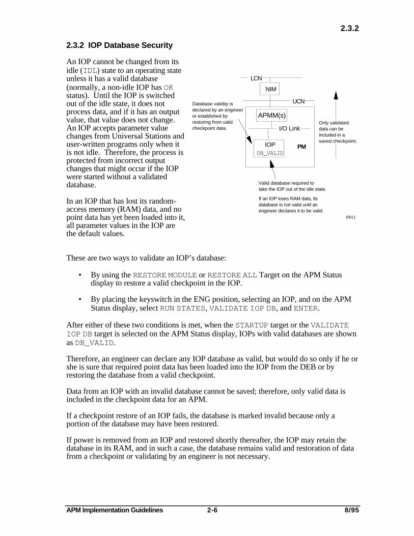
An IOP cannot be changed from itsidle (IDL) state to an operating stateunless it has a valid database(normally, a non-idle IOP has OKstatus). Until the IOP is switchedout of the idle state, it does notprocess data, and if it has an outputvalue, that value does not change.An IOP accepts parameter valuechanges from Universal Stations anduser-written programs only when itis not idle. Therefore, the process isprotected from incorrect outputchanges that might occur if the IOPwere started without a validateddatabase.

In an IOP that has lost its random-access memory (RAM) data, and nopoint data has yet been loaded into it,all parameter values in the IOP arethe default values.

Only validated data can be included in a saved checkpoint.

IOPDB_VALID

I/O Link

APMM(s)

NIM

UCN

LCN

PM

Valid database required totake the IOP out of the idle state.

Database validity isdeclared by an engineer or established by restoring from validcheckpoint data.

If an IOP loses RAM data, its database is not valid until an engineer declares it to be valid.

6911

These are two ways to validate an IOP’s database:

• By using the RESTORE MODULE or RESTORE ALL Target on the APM Statusdisplay to restore a valid checkpoint in the IOP.

• By placing the keyswitch in the ENG position, selecting an IOP, and on the APMStatus display, select RUN STATES, VALIDATE IOP DB, and ENTER.

After either of these two conditions is met, when the STARTUP target or the VALIDATEIOP DB target is selected on the APM Status display, IOPs with valid databases are shownas DB_VALID.

Therefore, an engineer can declare any IOP database as valid, but would do so only if he orshe is sure that required point data has been loaded into the IOP from the DEB or byrestoring the database from a valid checkpoint.

Data from an IOP with an invalid database cannot be saved; therefore, only valid data isincluded in the checkpoint data for an APM.

If a checkpoint restore of an IOP fails, the database is marked invalid because only aportion of the database may have been restored.

If power is removed from an IOP and restored shortly thereafter, the IOP may retain thedatabase in its RAM, and in such a case, the database remains valid and restoration of datafrom a checkpoint or validating by an engineer is not necessary.


3

BUILDING POINTSSection 3

This section defines the UCN node entities (points), node-specific entities (points), and processdata points that must be built and loaded into the APMs.

3.1 BUILDING UCN AND NODE-SPECIFIC POINTS

A UCN point must be built for each node on aUCN, including each NIM, each APMM, andany redundant partners. Also, you must build anode-specific point for each APMM and eachother node on the UCN. The UCN and LCNpoints are reserved entities. These entities mustbe built and loaded before data points can beloaded into the nodes on the UCN.

These entities are built with the Data EntityBuilder. After you select NETWORKINTERFACE MODULE on the Engineering MainMenu, select the UCN NODE CONFIGURATIONand NODE SPECIFIC CONFIGURATION picksto access the Parameter Entry Displays (PEDs)used to build them. For information about thevalues to be entered, refer to the AdvancedProcess Manager Parameter Reference Dictionaryin the Implementation/Process Manager - 2binder.

LCN

NIMNIM01

NIM02

100911

UCN

1312

14

02

Process networknumber for thisUCN (0 - 20)

3775

For the UCN example in sketch above, the following reserved entities would be built:

UCN Node UCN Point Node-Specific Point

NIM, UCN node no. 1 $NM02N01 N/ANIM, UCN node no. 2 $NM02N02 N/AAPMM (or other) node no. 9 $NM02N09 $NM02B09

. . .

. . .

. . .node no. 14 $NM02N14 $NM02B14

In the example above, NIM 01 and NIM 02 are partners in a redundant node pair. TheAPMMs can also be paired as redundant partners (for more information, see Section 2). AUCN point and a node-specific point must be built for each APMM and all redundantpartners.


3.2

3.2 DATA POINT BUILDING

Data points are also built with the Data Entity Builder. After selecting NETWORKINTERFACE MODULE on the Engineering Main Menu, select PROCESS POINTBUILDING.

The resulting menu allows you to choose one of several types of points, for exampleAnalog, Digital, Process Module, etc. Pulse Input points, and Smart Transmitter Interfacepoints are subsets of Analog Input points.

If you choose Regulatory PV or Regulatory Control points, an additional menu on thesecond page of these displays allows you to choose further sub-types of those points suchas Summer, Totalizer, PID, or Rampsoak points.

Process data point building consists of selecting options and entering parameters into theparameter entry screen displays and then loading the set of point specifications. Refer tothe APM Control Functions and Algorithms manual for information about each point type.Refer to the APM Parameter Reference Dictionary for parameter details. The SystemStartup Guide contains brief examples of data point building.

Points can only be loaded when the designated slot is in the inactive state, or the IOPcontaining the designated slot is in the Idle state. Points are loaded by selecting appropriatetargets on the Data Entity Builder’s Command Menu or from the Parameter Entry Displayby pressing a function key. The Process Operations Manual explains how to make pointsactive or inactive. Deleting a point leaves that slot active with default parameters as adatabase. Individual slots can be set to inactive status through the Slot Summary display.

You can either store a copy of the parameter entry data to an Intermediate Data File (IDF) orto an Exception Build file. The IDF store is easier, but the Exception Build file is moreadaptable for use in another system, or in later release software and the parameters can beedited using the Text File Editor. Refer to the Data Entity Builder Manual for theprocedures. Once the points are loaded and the database is set valid, the entire database canbe checkpointed (saved) in a format that is easily reloaded in mass.

While building points, you may need to specify I/O connections to other points. The otherpoints can be built as described above or they can be denoted as untagged (hardwarereference) points. An untagged point is built by specifying a syntax that refers to the IOPtype, IOP card number, slot number and parameter, all preceded by an exclamation point;for example, !AO12S03.OP. The complete format is explained in the APM ControlFunctions and Algorithms manual for applicable points. Untagged points are easy tospecify and do not deduct from the maximum NIM point count. The disadvantage is thatthey are relatively invisible in the system and operators or maintenance technicians may notbe aware of their presence. Therefore, you should keep careful records of the IOPs andslots where untagged points are implemented or use the Find Names utility to list them.Like tagged points, the slot must be inactive or the IOP idled to load them. You can checkthe slot status on the Slot Summary display.


3.3

3.3 RECONFIGURATION

There are several occasions when you may wish to reconfigure the APM data base:

• To add an IOP

• To delete an IOP

• To change from one IOP type to another

• To add control points

• To delete control points

• To change the scan rate

If you wish to replace an existing IOP with the same type (for example, a later revision), noreconfiguration is necessary. The IOP may be replaced with power on and the processrunning.

Note that changing from one IOP type to another amounts to deleting one IOP and addinganother. The various procedures are discussed in the following paragraphs.

Before starting you should —

• call up the UCN Status Display and fix any Soft Fail or Part Fail errors

• chekpoint the APM (save the data) to a cartridge and to the HM so that you can returnto the original configuration if necessary.

You will find it helpful to have the Command Processor Operation manual (for FindNames functions) and the Data Entity Builder manual (to reconstitute/load points/deletepoints) available. Section 7 in the Advanced Process Manager Service manual providesinformation on inserting and removing the physical IOP board.


3.3.1 To Add An IOP

The IOP card can be inserted with power on and the process running.

Then, reconstitute the Node Specific configuration file, NMnnBxx (where nn = theNetwork number and xx = the node number on the UCN). The procedure follows.

To reconstitute the Node Specific configuration file—

• Select NETWORK INTERFACE MODULE from the Engineering Menu

• Select NODE SPECIFIC CONFIGURATION from the NIM BUILD TYPE Menu

• Enter the desired Network Number and Node Number into the NODE SPECIFICCONFIGURATION display. If the word UNENTERED appears at the top, pressENTER until it disappears (repeat if necessary).

• Hold the CTRL key down and press 7.

The Parameter Entry Display should now contain a copy of the values that were loaded intothe system. The following steps change the values and reload the APM.

• Page forward to the IO MODULE CONFIGURATION section and make thenecessary changes (select IOP types and enter file/card numbers).

• To load the new configuration hold the CTRL key down and press ~ (F12)

• Hold the CTRL key down and press 9 (F9) to return to the NIM BUILD menu.

NOTE

If you added an SOE card, you must also reconstitute the NIM entityunder UCN NODE CONFIGURATION and set the TIMESYNC parameterto ENABLED. Then, reload the NIM entity as above.

• Select the Process Point Building target for the Point Build Menu. Choose a pointtype for the new IOP and configure points as needed.

• You can load each point by holding the CTRL key down and pressing ~ (F12) oryou can write each point to an IDF and then execute a LOAD MULTIPLE.

• Manually checkpoint to the HM (twice) and to the backup media (twice).


3.3

3.3.2 To Delete An IOP

For the IOP being removed—

• Make sure that no points exist for those slots. If you do not have adequate records,you can reconstitute each slot for that IOP and make a list. Note that this will notlocate hardware reference points (such as !DO03S05.SO). If you think hardwarereference points were built for for this IOP, try to find them using the Find Namesfunction (refer to the Command Processor manual).

• Use Find Names to determine where each point is used. Delete those point referencesin CL programs and schematics. They will have to be recompiled. Point referencesin the Area Data Bases must be deleted. You must reinstall the Area Data Base, but ifnew points will be added to either the area or schematics or CL programs, wait untilthat is done.

• Set each point in the IOP module to INACTIVE or• Set the IOP module to IDLE.

• Delete all points in the IOP.

• Reconstitute the Node Specific configuration file, NMnnBxx (see 3.3.1 for aprocedure) and change the IOP module to NONE. Or, if it is being replaced byanother IOP, this is the time to configure the new IOP type.

• To load the new configuration hold the CTRL key down and press ~ (F12).

• Hold the CTRL key down and press 9 (F9) to return to the NIM BUILD menu.

NOTE

If you deleted an SOE card, you must also reconstitute the NIM entityunder UCN NODE CONFIGURATION and set the TIMESYNC parameterto DISABLED. Then, reload the NIM entity as above.

• Manually checkpoint to the HM (twice) and backup media (twice).

The IOP card can be now be removed with power on and the process running.


3.3

3.3.3 Changing The Control Point Mix or Scan Rate

The point mix and the scan rate are configured as a part of the APM Box Data Point. Thisis viewed at the Universal Station, on the Node Specific Configuration display. These arethe choices for Regulatory PV and Regulatory Control points, and the flag, logic, numeric,digital composite points, etc. preceding the SCANRATE parameter on the configurationdisplay. SCANRATE refers to the Regulatory/Logic point scan cycle (REG1LOG1, etc.).

To change the point mix and/or the scan rate—

• Set the APM to IDLE. If you can access the UCN Status display from another US,this step can wait until you are ready to load the new configuration.

• If you are deleting control points, use the Find Names function to determine wherethose points are used (refer to the Command Processor manual). Delete the pointreferences in CL programs and schematics.

• Create a Selection List of all APM control points (but not IOP resident points).Aselection list is just a list of points in a file. For the procedure, refer to Section 7 inthe Data Entity Builder Manual. The UCN Status Display's Point Summary List,your IDF files, and good records can help you to build the Selection List.

• Using the Selection List created above, either Reconstitute Multiple to an IDF file, orPrint System Entities to an exception build file. Section 7 in the Data Entity BuilderManual describes these procedures. In brief, select the Command Menu. Then*—

To Reconstitute to an IDF file—

Select Reconstitute MultipleEnter a Reference Path Name (for example NET>nnnn>)Enter a pathname for the IDF file (for example CTLPNTS.DB)Enter the pathname name for your Selection List (for example SLIST.EL)Press Enter. Wait for the operation to complete.

To Print System Entities to an Exception Build file—

Select Print EntitiesSelect Print System EntitiesEnter a Reference Path Name (for example NET>nnnn>)Enter the pathname name for your Selection List (for example SLIST.EL)Enter a Destination pathname for the exception build file (for example EXFILE.EB)Press Enter. Wait for the operation to complete.

The IDF file (.DB ) or the Exception Build file (.EB) will be used later to reload thecontrol points.

*For the examples shown, when you only specify a file name, the Reference Path Name isprefixed to form a complete path name. If any files are on removable media, specify thefull path name.


3.3

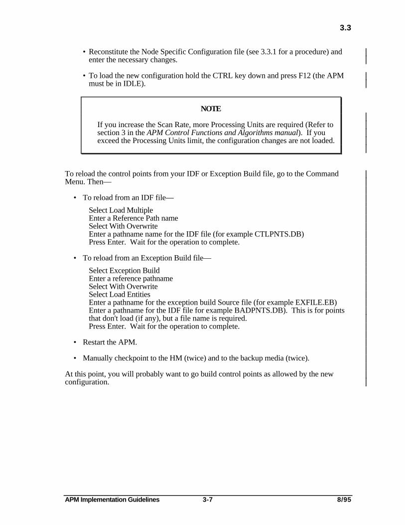
• Reconstitute the Node Specific Configuration file (see 3.3.1 for a procedure) andenter the necessary changes.

• To load the new configuration hold the CTRL key down and press F12 (the APMmust be in IDLE).

NOTE

If you increase the Scan Rate, more Processing Units are required (Refer to section 3 in the APM Control Functions and Algorithms manual). If you exceed the Processing Units limit, the configuration changes are not loaded.

To reload the control points from your IDF or Exception Build file, go to the CommandMenu. Then—

• To reload from an IDF file—

Select Load MultipleEnter a Reference Path nameSelect With OverwriteEnter a pathname name for the IDF file (for example CTLPNTS.DB)Press Enter. Wait for the operation to complete.

• To reload from an Exception Build file—

Select Exception BuildEnter a reference pathnameSelect With OverwriteSelect Load EntitiesEnter a pathname for the exception build Source file (for example EXFILE.EB)Enter a pathname for the IDF file for example BADPNTS.DB). This is for points that don't load (if any), but a file name is required.Press Enter. Wait for the operation to complete.

• Restart the APM.

• Manually checkpoint to the HM (twice) and to the backup media (twice).

At this point, you will probably want to go build control points as allowed by the newconfiguration.


4

NIM LOADING AND PERFORMANCESection 4

This section describes methods for estimating Network Interface Module loading and assessingthe results of your estimates. Also described is the implementation of a second NIM (or NIM pair)on a UCN, to share the processing load.

4.1 ESTIMATING NIM LOADING

Tables 4-1 and 4-2 provide an example of NIM loading estimates for the NIM in aperformance cluster with one APM on the UCN, three Universal Stations, one HistoryModule, and one Application Module, (for more information about a performance cluster,refer to the Engineer’s Reference Manual). The HM contains APM checkpoints andcontinuous history.

The Universal Stations are used to view standard displays and two custom schematics.Each custom schematic contains 250 parameters, 50 of which are on fast update. Refer toTable 4-3 for added schematic Load Factors. Refer to the Set Collection command in thePicture Editor Reference Manual for more information on fast update.

Use Table 4-1 for systems with a 68020 NIM and Table 4-2 for systems with a 68040NIM. 68020 and 68040 refer to the NIMs microprocessor type. If the NIM contains aK4LCN board, it is a 68040 NIM. If not, it is a 68020 NIM.

A NIM load estimate is calculated by multiplying the value you entered in the Numbercolumn by the factor in the Load Factor column, entering the results in the Induced Loadcolumn, and adding the values in the Induced Load column. Comments following thetables explain more about the considerations. In the first example, the total induced load is625, which is 62.5% of the maximum load allowed for a NIM.

You should make a loading estimate for each NIM in your system. If you have severalNIMs, consider using a spread sheet on a personal computer to do your calculations. Thefollowing comments along with Tables 4-1 and 4-2 help to further explain the process:

General —

• Indicate the number of active LCN nodes, that is, those that are principally accessinginformation from the UCN resident devices. For the History Module, this meanscontinuous history. Then apply the load factors as explained below.

• Redundant Nodes—Count redundant node pairs (NIMs, AMs, APMMs, HPMMs,PMMs, LMs and SMs) as one node.


4.1

Table 4-1 — 68020 NIM Loading EstimatorUnits to be entered Load Induced

Load Sources in Number column Number Factor Load

US Induced Load

Universal and UXS Stations Number principally accessing this NIM 3 15 45

Fast Schematic Displays Number principally accessing this NIM 2 85 170

UCN Induced Loads

PMs, APMs, HPMs, LMs Number of PMs, APMs, HPMs, LMs 10 10 100and/or SMs on the UCN and SMs on the UCN

History Module Induced Load

Continuous History:

68020 HM Number of HMs principally accessing 1 30 30 (2400 Points per minute) this NIM

68040 HM Number of HMs principally accessing 0 40 (3000 Points per minute) this NIM

Checkpoints Number of HMs checkpointing this NIM 1 70 70

AM and AXMs Induced Loads (90 Points/second)

AMs with 68020 microprocessor Number principally accessing this NIM 1 150 150

AMs with 68040 microprocessor Number principally accessing this NIM 0 200

CG Induced Loads

Computer Gateways Number principally accessing this NIM 1 60 60 (100 parameters/second)

Total Induced Load: 625Maximum Allowable Load: 1000

% of maximum allowable load: 62.5


4.1

Table 4-2 — 68040 NIM Loading EstimatorUnits to be entered Load Induced

Load Sources in Number column Number Factor Load

US Induced Load

Universal and UXS Stations Number principally accessing this NIM 3 6 18

Fast Schematic Displays Number principally accessing this NIM 2 35 70

UCN Induced Loads

PMs, APMs, HPMs, LMs Number of PMs, APMs, HPMs, LMs 10 4 40and/or SMs on the UCN and SMs on the UCN

History Module Induced Load

Continuous History:



Checkpoints Number of HMs checkpointing this NIM 1 28 28

AM and AXMs Induced Loads (90 points/second)



CG Induced Loads

Computer Gateways Number principally accessing this NIM 1 24 24 (100 parameters/second)

Total Induced Load: 276Maximum Allowable Load: 1000

% of maximum allowable load: 27.6


4.2

Schematics—

• Assume that the schematics are principally accessing this NIM.

• For every Universal Station there is a base load factor as shown in Table 4-1or 4-2. Add to this the load factor from Table 4-3 —

Table 4-3— Schematic Load FactorTotal Parametersin Schematic

Number of Parameterson Fast Update

Added LoadFactor 68020

Added LoadFactor 68040

100 0 0 0100 50 65 26150 0 5 2150 50 70 28200 0 15 6200 50 75 30250 0 20 12250 50 85 34

HMs—• The checkpoint load factor is in addition to the History Module factor. The 68020

HM Continuous History load factor is based on a HM with a 68020 processorcollecting history for 2400 points per minute. The 68040 HM Continuous Historyload is based on a HM with a 68040 processor collecting history for 3000 points perminute.

AMs and AXMs—

• The AM load factor is based on a fully-loaded AM accessing data from this NIM.A fully loaded 68020 AM processes 90 points per second. A fully loaded 68040 AM processes 120 points per second.

CGs—• The CG load assumes that it is requesting 100 parameters per second from the NIM.

4.2 ASSESSMENT OF NIM LOADING

The following are the NIM loading categories:

• A NIM whose total induced load is 750 (75%) or less can be expected to perform asspecified under all actual system-use conditions.

• If the total induced load is between 750 and 1000 (75% to 100%), the NIM load ismarginally acceptable, and display of information from this NIM and its reportingof events may occasionally be sluggish, especially during a process upset or a peakload such as multiple point loading.

• If the total induced load is above 1000 (100%), the NIM should be consideredoverloaded, and should a failover to the backup NIM or some other system upsetoccur, the view to the process may be temporarily lost.


4.3.

4.3 USE OF A “REMOTE” NIM TO SHARE PROCESSING LOAD

An additional NIM (redundant NIM pair) can be added to the UCN and the LCN to sharethe processing load with another NIM. To use such a NIM, you must adhere to certainrules for point assignments and operational practices.

4.3.1 Implementation of Two Logical Process Networks

From the LCN viewpoint, the two NIMs(redundant NIM pairs) are on separateprocess networks, even though they areconnected to the same physical UCN. Thefirst NIM (configured as ThisNIM) isassigned to process network n (n is in arange from 1 to 20; each UCN and eachData Hiway is one process network) andthe second NIM (configured asRemotNIM) is assigned to process networkn+1. The assignment of the networknumbers is arbitrary, but consistent, logicalassignment simplifies operating practices.

LCN

NIM NIM

LCN nodes see two logical UCNs

One physical UCN3776

The NIMs to be configured as ThisNIM and RemotNIM and their process networks mustfirst be defined in the NCF through the Engineering Personality’s LCN NODES activity.Then, all of the UCN nodes, including the NIMs, are defined on both process networks bybuilding UCN entities (NIM points) and Node Specific entities (box points). In the UCNNode entities, about half of the nodes on each process network are configured withNODEASSN = ThisNIM and the remainder with NODEASSN = RemotNIM. Each nodeassigned as ThisNIM on process network n is assigned as RemotNIM on n+1, and eachnode assigned as ThisNIM on process network n+1 is assigned as RemotNIM onnetwork n.


4.3.1

For example, for the UCN node numbersin this sketch, you would build thefollowing UCN node and node-specificentities:

52283/Rev

LCN

NIM NIM

APM 05

LM 06

NIMs 01 and 02NIMs 03 and 04

Logical UCNs 01 and 02

NodeUCN Entity Specific

Node UCN Name NODEASSN Ent. Name

NIM 01 01 $NM01N01 ThisNIM N/ANIM 02 01 $NM01N02 ThisNIM N/ANIM 03 01 $NM01N03 RemotNIM N/ANIM 04 01 $NM01N04 RemotNIM N/A

APM 05 01 $NM01N05 ThisNIM $NM01B05LM 06 01 $NM01N06 RemotNIM $NM01B06

NIM 01 02 $NM02N01 RemotNIM N/ANIM 02 02 $NM02N02 RemotNIM N/ANIM 03 02 $NM02N03 ThisNIM N/ANIM 04 02 $NM02N04 ThisNIM N/A

APM 05 02 $NM02N05 RemotNIM $NM02B05LM 06 02 $NM02N06 ThisNIM $NM02B06

As you build process points to reside on the two logical UCNs, assign approximately equalnumbers of points to each UCN (parameter NTWKNUM), but take care to assign pointsthat use peer-to-peer communication to the same UCN (peer-to-peer communication isthrough connections from points in one logical UCN node to points in other nodes on thesame logical UCN).

NOTE

All nodes must be assigned to both UCNs (some local, some remote). This is necessary toassure proper UCN cable handling.


4.3.2

4.3.2 Operational Considerations for Two Logical Process Networks

Use of the SAVE DATA target to checkpoint data from the UCN nodes and the restorationof checkpoint data to the nodes can be accomplished only from the UCN Status display forthe process network the nodes are assigned to (NODEASSN = ThisNIM). If you try fromthe wrong display, a “node assignment” error message appears. If some of the points in aUCN node are assigned to process network n and others are assigned to process networkn+1, you will have to use SAVE DATA twice, once from each UCN Status display.

For automatic checkpointing to save all data, it must be enabled through the UCN Statusdisplays for both process networks and for each UCN node to be auto-checkpointed.

Alarming, message transfers, and event-initiated processing are handled by the NIMs andno special operational considerations are required.

4.3.3 Functional Relationships of Two Logical Process Networks

Successful implementation and use of two NIMs and logical process networks that shareprocessing loads is more likely if you understand the relationships described here.

The UCN node configuration establishes the relationships of the two NIMs (or two pairs ofredundant NIMs) and the two logical process networks. For example, NIMs are assignedto the appropriate UCN through configuration.

The relationships of APMs to the NIMs is defined in the UCN node point parameterNODEASSN, which contains either ThisNIM or RemotNIM. Two UCN node entities areconfigured for each UCN node, one on each process network. The APM’s points areprocessed by the NIM on the process network for which the APM's NODEASSN value isThisNIM.

UCN nodes configured with NODEASSN = RemotNIM appear on the UCN Status displayfor the process network associated with the NIM that is not processing their points, eventhough they don’t logically belong to that network. The boxes for UCN nodes thatlogically belong to a process network are green and the boxes for nodes that logicallybelong to the other process network are yellow.

Because process points are assigned to a process network as the points are built, an APM,can contain points that belong to one network and other points that belong to the othernetwork. A point’s database resides partly in the APM and partly in the NIM that has thesame process network assignment as the point.

Consider this checkpointing example for process networks 1 and 2: when the data for anAPM is checkpointed, all point data for the APM is saved in the checkpoint directory forprocess network 1, but the NIM-resident data for the points assigned to network 2 is notsaved until another checkpoint operation saves the data for network 2 in the directory forthat network.


5

SERIAL DEVICE INTERFACE IMPLEMENTATIONSection 5

This section describes methods to connect various devices to the Advanced Process Managerthrough a Serial Device Interface.

5.1 GENERAL IMPLEMENTATION INFORMATION

The Serial Device Interface (SDI) allows various devices to be easily connected to theAPM. Field Termination Assemblies (FTA) connected between the device(s) and the SDII/O Processor (IOP) contain firmware to map the device data so that it mimics data from aSmart Transmitter. Each type of device uses a corresponding type of FTA designed toprocess the I/O and return any status or control signals required by that type of device.

The SDI IOP itself must be configured as a Smart Transmitter Interface module (STIM).Note that up to two SDI FTAs can be connected to each SDI IOP. The first FTA uses thefirst 8 STI points; the second uses STI points 9 – 16. Each FTA can support one specificdevice type.

The following standard interfaces are currently supported:

• Manual Auto Station• Toledo Weigh Scale, Models 8142-2089• Toledo Weigh Scale, Models 8142-2189• UDC 6000 Process Controller

Other SDI Interfaces are being developed. Contact Honeywell for more information.

Section two of the Advanced Process Manager Control Functions and Algorithms manualdescribes the characteristics, constraints, and operating considerations for SDI options. Italso provides charts showing how the critical parameters relate between the APM and theserial device.

The remainder of this section discusses the unique implementation of each Serial DeviceInterface option.


5.2

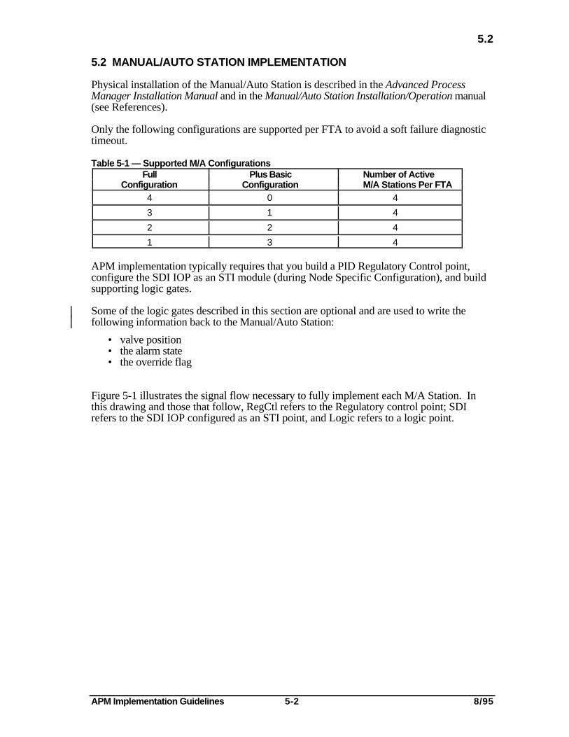
5.2 MANUAL/AUTO STATION IMPLEMENTATION

Physical installation of the Manual/Auto Station is described in the Advanced ProcessManager Installation Manual and in the Manual/Auto Station Installation/Operation manual(see References).

Only the following configurations are supported per FTA to avoid a soft failure diagnostictimeout.

Table 5-1 — Supported M/A ConfigurationsFull Plus Basic Number of Active

Configuration Configuration M/A Stations Per FTA4 0 4

3 1 4

2 2 4

1 3 4

APM implementation typically requires that you build a PID Regulatory Control point,configure the SDI IOP as an STI module (during Node Specific Configuration), and buildsupporting logic gates.

Some of the logic gates described in this section are optional and are used to write thefollowing information back to the Manual/Auto Station:

• valve position• the alarm state• the override flag

Figure 5-1 illustrates the signal flow necessary to fully implement each M/A Station. Inthis drawing and those that follow, RegCtl refers to the Regulatory control point; SDIrefers to the SDI IOP configured as an STI point, and Logic refers to a logic point.


5.2.1

SDI.PVTV

(Aux.)

STI(SDI)

Logic(Primary)

SDI.LRV

SDI.URV

RegCtl

(PID)

SDI.CJTACTRegCtl.SP

RegCtl.OP

RegCtl.AUTMODF

Logic

Box Numeric(Valve Pos.)

Box Numeric(Alm. State)

Box Numeric(Override)

FTA

FTA

To/FromM/A Stations

SDI.DAMPINGSDI.PIUOTDCF

RegCtl.PV

RegCtl.OPRegCtl.SPPRegCtl.ESWMANRegCtl.ESWAUTO

SDI.URL

SDI.PVRAWSDI.SECVARSDI.STI_EU

Optional

RegCtl.ESWENBSTRegCtl.ESWCAS

Figure 5-1 — Manual/Auto Station Implementation Strategy 11327/Rev

5.2.1 Input Functions from the Manual/Auto Station

Signals sent from the Manual/Auto Station include mode change requests, also Setpoint andOP change requests along with the Setpoint and OP values. The configuration needed tohandle these signals is discussed in the following paragraphs.

5.2.1.1 Setpoint and Mode Change Requests

The Manual/Auto Station request for an SP, OP, or mode change is determined by a changein the value of parameter STI_EU. Figure 5-2 shows how the primary logic point in theAPM is configured with a series of “Equals” blocks to detect values of 1, 3, or 4. Thevalue of STI_EU is normally 0, but temporarily changes to 1 through 4 depending on therequest (refer to the Advanced Process Manager Control Functions and Algorithmsmanual).


5.2.1

A Setpoint change request causes SO1 to enable the PVRAW value through logic blockOutput 1. PVRAW is the desired setpoint from the Manual/Auto Station.

When there is a manual or auto mode change request from the Manual/Auto Station,STI_EU enables SO3 or SO4, respectively, to turn on the appropriate external switchingflag to the regulatory control point.

EQ S01

From M/A Station

SDI.STI_EU

NN(1) = 1

SDI.PVRAWRegCtl.SPP

To RegCtl Point

Out 1

Enable

RegCtl.ESWMANS03

NN(3) = 3 EnableOut 5

FL2 (On)

EQS04

NN(4) = 4

RegCtl.ESWCAS

FL2 (On)

SDI.STI_EU

SDI.STI_EUOut 6

Enable

Enable

Out 11

Enable

Out 13

ONDLY RegCtl.ESWAUTO

FL2 (On)

DLYTIME = 1 Out 12

Enable

FL2 (On)

RegCtl.ESWNBST

FL2 (On)

RegCtl.ESWENBST

EQ

Figure 5-2 — Setpoint and Mode Change Request Strategy, APM New

5.2.1.2 OP Change Requests

In an APM, the mode attribute parameter (MODATTR) for the regulatory control pointmust be set to PROG before the OP parameter can be changed by a logic point.Figure 5-3 shows the strategy. When the STI_EU parameter’s value equals twoindicating an OP change request, logic gate SO2 triggers logic gate Out 4 setting themode attribute to PROG. The ONDLY gate then enables the requested OP value in theSECVAR parameter through gate Out 2. Finally, as ONDLY turns off, gate Out 3switches the mode attribute back to OPER. Figure 5-4 illustrates the timing.


5.2.1

From M/A Station

SDI.SECVAR RegCtl.OP

To RegCtl Point

Out 2

Enable

EQS02

SDI.STI_EU

NN(2) = 2

RegCtl.MODATTR

Out 3

EnableANDS07

N

FL2 (On)

ONDLY OFFDLYS06

Out 4

Enable

RegCtl.MODATTR

S05

NN(1) = 1

NN(2) = 2

(PROG)

(OPER)

Figure 5-3 — OP Change Request Strategy, APM 11333

S02

S05

S06

S07

Out 4, MODATTR = PROG.

Out 3, MODATTR = OPER

Write New OP

Figure 5-4 — APM OP Request Strategy Timing 11332


5.2.2

5.2.2 Output Values and Control Functions Sent to the Manual/Auto Station

Signals sent back to the Manual/Auto Station for display purposes include the mode,the Setpoint, and OP. An auxiliary logic point can be used to send the Override Flag,alarms, and the valve position.

5.2.2.1 Fundamental Signals Sent to the Manual/Auto Station

Figure 5-5 illustrates how the Setpoint, PV, OP, and mode flag from the regulatorycontrol point are written back to the Manual/Auto Station using logic gates.

To M/A Station

SDI.PVTV

From RegCtl Point

Out 7

Enable

FL2 (On)

Out 8

Enable

EnableFL2 (On)

SDI.LRV

SDI.URL

EnableFL2 (On)

SDI.CJTACT

FL2 (On)

RegCtl.SP

RegCtl.PV

RegCtl.OP

RegCtl.AUTMODF

Out 9

Out 10

(Setpoint)

(PV)

(OP)

(Auto Mode flag)

Figure 5-5 — Values written to M/A Station 11334


5.2.3

5.2.3 Additional Logic Implementation

The logic functions described in this section are optional but provide useful functions.

5.2.3.1 Optional Logic Implementation

Some additional logic can be used to feed back the override flag, alarm status, and valveposition to the Manual/Auto Station. Figure 5-6 illustrates how these signals can bereturned to the Manual/Auto Station.

To M/A Station(via SDI IOP)

SDI.PIUOTDCFFrom Separate Box Flag

Out 1

Enable

FL2 (On)

Out 2

Enable

EnableFL2 (On)

SDI.DAMPING

SDI.URV

FL2 (On)

MAOVRFLG.PVFL

MAALM.PV

MAVPOS.PVOut 3

(Override Flag)

(alarm level)

(Valve Position)

From Separate Box Numeric

From Separate Box Numeric

Figure 5-6 — Auxiliary Logic Point Implementation 11335


5.2.3

5.2.3.2 Alternative Alarming Strategy

Figure 5-7 illustrates an alarming scheme whereby the PV High and Low Alarm Flagscan be used to feed back PV out-of-range alarms to the Manual/Auto Station. PVHIFLon alone sets alarm 1, PVLOFL on alone sets alarm 2, and alarm 3 is set when bothare on (this is an alternative to using logic gate Out 2 as shown in Figure 5-6).

ANDS01

To M/AStation

NN(1) = 0

SDI.DAMPING

From RegCtl Point

Out

Enable

S02

NN(2) = 1

Enable

S03

NN(3) = 2 Enable

S04

NN(4) = 3 Enable

RegCtl.PVHIFL

N

N

N

N

RegCtl.PVLOFL

AND

AND

AND

SDI.DAMPING

SDI.DAMPING

SDI.DAMPING

Out

Out

Out

Figure 5-7 — PV Out-Of-Range Strategy 11336


5.3

5.3 WEIGH SCALE IMPLEMENTATION

5.3.1 Methods of Control

The model 8142-2089 or 8142-2189 Toledo Weigh Scale can be controlled through a CLprogram or schematic (or both). In this section, a simple example is provided to show howa schematic could be used.

5.3.2 Control Schematic Example

Figure 5-8 shows a simple schematic for Toledo Weigh Scale control using the SerialDevice Interface. This schematic is a simple example to show the approach and may not besuitable for actual control. Figure 5-8 shows how the schematic appears in the PictureEditor and provides some formatting information.

SCALE 1

SCALE 2

SCALE 3

SCALE 4

Point

Setpoint

ChangeSetpoint

Flow Rate

Flow Rate Limit

Set Rate Limit

Scale Status

Weight

Cutoff Weight

Feed Status

StartFeeding

Point Status

Set Point Active

Set Point Inactive

Mode =

ON

ASCENDING

Scale No.1GGGGGGGG=

RRRRRRRRR RRRRRRRRR

RRRRRRRRR

RRRRRRRRR

RRRRRRRRR

EEEEEEEEEE=

TTTTTTTTTTTTTTTTTTTTTTTTTTTTTTTTTTTTTTTTTTTTTTTTTTTT

Figure 5-8 — Weigh Scale Schematic Example 11330

The following comments explain how the schematic is used—

• One of the four scales is selected.

• A weight setpoint value is sent to the scale.

• When Start Feeding is selected, feed control is turned on. When the weight hasreached the setpoint value, the feed is turned off automatically at the scale. Feedstatus, weight, flow rate, etc., are reported through value objects on the screen.


5.3.2

Figure 5-9 shows the targets. Action sequences are shown in italics.

S_ENT(ENT01,SDI104);S_INT(INT01,04)


SCALE 1

SCALE 2

SCALE 3

SCALE 4

POINT

Set Rate Limit

Set Point Active

Set Point Inactive

S_ENT(ENT01,SDI101);S_INT(INT01,01

Target Action:

Target Action:

Target Action:

Target Action:

Target Action:SS_REAL(ENT01.PVTV,R_REAL(14,18,9, "ENTER SETPOINT",TRUE,0))

SS_REAL(ENT01.URL,R_REAL(14,12,9, "ENTER RATE LIMIT",TRUE,0))

StartFeeding

Target Action:SS_BOOL(ENT01.CJTACT,ON)

SS_ENM(ENT01.PTEXECST,"ACTIVE")

SS_ENM(ENT01.PTEXECST,"INACTIVE")

Target Action:

ChangeSetpoint

Target Action: (invisible)Detail (IE_ENT(ENT01))

Initial Target: DEFINE INITTarget Action: same as for SCALE 1.

Target Action: Target Action:


=

Figure 5-9 — Weigh Scale Schematic Targets 11329


5.3.2

Figure 5-10 shows the values, variants, and conditional behavior.

SCALE 1

SCALE 2

SCALE 3

SCALE 4

Point =

Setpoint

Flow Rate =

Flow Rate Limit

Scale Status

Weight

Cutoff Weight

Feed Status

StartFeeding

Point Status =

Set Point Active

Set Point Inactive

ENT01.PVTV

ENT01.SECVAR

ENT01.PV

ENT01.LRL

ENT01.PTEXECST

ENT01.S1

ChangeSetpoint

Set Rate Limit

ENT01.URL

Mode = Variant:IF ENT01.PIUOTDCF = ONTHEN "ASCENDING" ELSE "DESCENDING"

ON

ASCENDING

— —

Condition:IF ENT01.CJTACT=ONTHEN SET YEL BLINKELSE SET CYAN NO BLINK

ENT01.NAMEScale No. 1

Variant:IF INT01= 01 THEN "1"ELSE IF INT01=02 THEN "2" ELSE IF INT01=03 THEN "3 "ELSE "4"

=

Condition:IF INT01=01THEN SET YEL ELSE SET CYAN




ENT01.CJTACT

Figure 5-10 — Weigh Scale Schematic Values and Variants 11331


5.3.2

5.3.2.1 Control Schematic Description

To understand the control, you should refer to the table of Weigh Scale/STI parameters inthe Advanced Process Manager Control Functions and Algorithms manual. For help inunderstanding Picture Editor functions, refer to the Picture Editor Reference Manual.

The following comments help to explain the example schematic—

• Upon invoking the schematic, an initial target selects Scale 1 as described below.This guarantees that the DDB variables contain acceptable starting values.

• Selecting one of the four scale targets loads the DDB Entity ENT01 with the properpoint reference. It also loads the DDB Integer INT01 with the scale number1, 2, 3, or 4. Conditional behavior changes the selected target from white to yellow.

• At the top of the schematic, a value displays the contents of ENT01 to show thepoint name. A variant tests INT01 and displays the selected scale number. An invisible target over the word: Point = is provided call up the detail display if needed.

• The Change Setpoint and Set Rate Limit targets open ports for an operator to typein desired values.

• The Start Feeding target stores ON for parameter CJTACT to turn the feed on.A value displays the text: ON after the words Feed Status. Below the wordON, a text line turns yellow and blinks when a conditional behavior test findsCJTACT = ON. When the setpoint is reached and feed is stopped at the scale, CJTACT returns to Off. OFF is displayed for the Feed Status and the line returns to steady state cyan.

• A variant tests parameter PIUOTDCF and displays ascending or descending mode.If you need to change the mode, you can do so at the Detail Display.


5.3.2

5.3.2.2 Point Configuration

A typical STI point configured for use with the schematic is shown in Table 5-5. Defaultvalues are acceptable in most cases. Some output values are set to 0 and some controlparameters are initially configured to OFF for safety. Ascending weight is assumed; ifdescending is desired, set PIUOTDCF to OFF.

Use your own point name, unit number, network, node, and slot numbers. Use defaultvalues for parameters not included. The last four entries contain required values.

Four points, (SDI101 through SDI104) were built for use in this example to show howfour scales could be controlled. Configuration of the points was the same except for thename and slot number. Because each scale is connected to a separate FTA, scales 3 and 4require a second SDI IOP and its two associated FTAs.

Table 5-5 — APM STIM (SDI) PointParameter Entry

NODETYP APMPNTFORM FULLPNTMODTY STIMSENSRTYP STTPVCHAR LINEARSTI_EU MVDECONFLRV 1URL 0DAMPING 0PIUOTDCF ON (Ascending)CJTACT OFFINPDIR DIRECTPVEUHI 100.0 (Required)PVEULO 0.0 (Required)PVEXEUHI 100.0 (Required)PVEXEULO 0.0 (Required)

5.3.2.3 Schematic Enhancements

You could add a drawing of a scale and insert parameters in appropriate places.

Some functions can be eliminated and others could be added. For example, if you onlyhave one scale, eliminate the Point and Scale identifiers and the scale targets. Substitute thepoint ID in all expressions for ENT01. You may want to add a target to call the DetailDisplay for that point.

If you need to change from ascending to descending mode frequently, that functionalitycould be built into the schematic.

You can build the scale targets into another schematic to call a subpicture with scale controlfunctions.


5.4

5.4 UDC 6000 Process Controller

5.4.1 Overview

The UDC 6000 Controller is a stand-alone single loop controller. Up to four UDCControllers can be connected through each of the two FTAs to an SDI IOP.Communication uses the EIA-485 protocol.

Refer to PM12-520, the PM/UDC 6000 Integration Manual for configuration informationand references to other UDC 6000 publications.


6

PEER-TO-PEER COMMUNICATION AND PERFORMANCESection 6

This section discusses Peer-to-Peer Transaction Throughput constraint in terms that allowgeneral estimates on system capability to be made before implementation of the overallcontrol strategy has been carried out. A description of the performance statistics andmethods that can be used to troubleshoot performance problems are included.

6.1 SYSTEM CONSTRAINTS ON PEER-TO-PEER COMMUNICATION

System constraints limit the quantity of data that can be transported between peer APMs.These constraints include limits on

• the number of parameters that can be passed using specific transport mechanisms(configuration limits).

• the total number of parameters that can be serviced in each second (ParameterThroughput).

• the number of transactions that can be processed each second (TransactionThroughput).

6.1.1 Configuration Limits

Peer to peer configuration limits are discussed in Section 3 of the Control Functions andAlgorithms Manual.

6.1.2 Parameter Throughput Limit

The limit on Parameter Throughput in the APM has been estimated at 400 parameters persecond. The sum of all parameter requests to any individual APM should not exceed thisvalue.

While it is important that system configuration not exceed this limit, previous experienceindicates that the Transaction Throughput limit discussed below is usually reached first.

6.1.3 Transaction Throughput Limit

When parameters are transported over the UCN, they are sent in groups called messages.Two kinds of messages are involved: request messages and response messages.

• Request messages are those sent by the node that wants the data to the node that ownsthe data. They list all the parameters to be transported.

• Response messages are sent by the node that owns the data to the node that requestedthe data. They contain the actual parameter values.


6.2

All parameter transport requires a complete cycle of message request and messageresponse. Such a cycle is called a transaction. Note that transactions occur when peernodes communicate and also when NIMs and PMs/APMs communicate in response toLCN initiated requests.

The rate at which transactions occur is called the Transaction Throughput. Like ParameterThroughput, it is one component of the overall load on the APM. In most applications,Transaction Throughput is a more important component of load than ParameterThroughput.

Lab measurements have shown that in most configurations, the APM can handle 50transactions per second.

In general, when a peer-to-peer configuration is designed, it should target a TransactionThroughput at or below 50 for steady-state and peak-load conditions alike. However, ifthis limit is exceeded by small amounts at infrequent intervals, the effect is small. UCNoverruns result and some of the peer transactions will slow down.

Large and frequent overrun counts or UCN overrun soft failures are signs that TransactionThroughput is too heavy.

Cases where 50 transactions per second is too much—Certain configurations can havecommunications overruns at Transaction Throughput loads below 50.

CAUTION

Application engineers should be particularly cautious if a significant number of peer-to-peer connections make reference to IOP resident data.

The APM peer-to-peer communication capability is primarily intended to support transportof Control Processor resident data. If large amounts of IOP owned data must betransported, they should first be fetched into the Control Processor by a local connection.The peer-to-peer connections can then reference the data from its Control Processorlocation.

6.2 LOCAL AND REMOTE DATA

In the following discussion, Transaction Throughput values are always quoted in units oftransactions per second.

Imagine a UCN with P + 1 APM nodes operating as peers and one NIM node connected tothe LCN (see Figure 6-1).

For an APM called ME, data transactions can be divided into two classes:

• those that transport remote data not owned by ME into ME• those that transport local data owned by ME into other nodes.


6.2

NIMAPMME APM 1 APM 2 APM n

LocalData

RemoteData

12478

Figure 6-1 — Local and Remote Data

Remote data can be transported by pulls (reads) from ME or by pushes (writes) from the Pother nodes. Similarly, Local data can be transported by pushes from ME or by pulls fromthe P other nodes. The distinction between remote and local has to do with who owns thatdata that is to be transported, not with whether pushes or pulls are used to effect thetransport.

For nodes that are exclusively data sinks, the peer-to-peer load is caused only by remotedata. For nodes that are exclusively data sources, the situation is reversed.

6.2.1 Transaction Load from Peer Traffic

Transaction load on ME, generated by the P peer APM nodes, depends strongly on twofactors:

• the number of other nodes communicating (P), and• the specific mechanisms used to transport data between ME and the peer nodes.

Node Count Effects—The dependence on P is linear.

Configuration Effects—The dependence on configuration is harder to characterize.Relevant factors include the following:

• ME is a data source, data sink, or both. If peer transactions transport only local data,ME is a pure source. If peer transactions transport only remote data, ME is a puresink. Using ME as both a source and a sink, typically doubles the transaction load.

• Data is transported by pulls, pushes, or both. Data transport to and from ME isaccomplished primarily by pull or push mechanisms, or by a combination of the two.It is advantageous to use exclusively one or the other.

• Data is transported by continuous points, sequence points, or both. Data transport toand from ME is accomplished primarily by continuous point mechanisms(connections configured in Regulatory PV, Regulatory Control, or Logic points), bysequence point mechanisms (Read and Write statements in Process Module Datapoints), or by a combination of the two. It is advantageous to use exclusively one orthe other.


6.2

6.2.2 Push/Pull Examples

The following examples illustrate the range of variation possible due to configurationoptions:

Example 1: Very Inefficient Transaction Usage

Both pushes and pulls are used to accomplish data transport. Both continuous and sequencepoint mechanisms are used.

Remote Transaction Load = 10 x PLocal Transaction Load = 10 x P

Example 2: Moderately Efficient Transaction Usage

Transport mechanisms are restricted to pushes. Both continuous and sequence mechanismsare used.



Transport mechanisms are restricted to pulls. Both continuous and sequence mechanismsare used.



Transport mechanisms are restricted to continuous mechanisms. Both pushes and pulls areused.



Transport mechanisms are restricted to sequence mechanisms. Both pushes and pulls areused.


Example 6: Efficient Transaction Usage

Only pulling is used for data transport. Only continuous mechanisms are used.


Figure 6-2 shows the dependence of transaction load on node count for each of the exampleslisted above. Each plot applies to transport of either remote or local data.


6.3

60

50

40

30

20

10

04 8 12 16 20 24

Ex. 1 Ex. 5 Ex. 6Ex. 2,3,4

Number of Other Nodes

Transmission Load(Transactions per Second)

Figure 6-2 — Transmission Throughput 12117

Note that for certain types of applications, even the approach used in example 6 mayimpose too much load. This is further described in subsection 6.5

6.3 TRANSACTION LOAD FROM NIM TRAFFIC

Transaction load imposed by the NIM upon ME can vary greatly depending on staticfactors such as LCN configuration. It also depends on dynamic factors such as:

• how many active displays draw data from ME• how many AM or CM strategies pull and push to ME• whether history data is being collected• how many events are being generated by ME.

To roughly characterize these variations, two categories of loads can be considered:

• typical• large


6.3.1

6.3.1 Typical NIM, Transaction Load = 8

This might be generated by an LCN with the following nodes and activities:

• one 68020 AM• one CM50 generating requests at its maximum rate• one HM generating requests at its typical rate• one group displays on fast update• one group displays on normal update• one schematic display of about 100 parameters• one detail display

6.3.2 Large NIM, Transaction Load = 21

This might be generated by an LCN with the following nodes and activities:

• two 68020 AMs• one CM50 generating requests at its maximum rate• one HM generating requests at its maximum rate• two group displays on fast update• two group displays on normal update• three schematic displays of about 100 parameters each• two detail displays

6.4 ESTIMATING TRANSACTION THROUGHPUT

Use the following procedure to estimate Transaction Throughput:

1. Identify how many APMs will be connected to the UCN.

2. Consider each APM one at a time thinking of it as the ME node.

3. Identify how many peer nodes will be communicating with ME (P).

4. Estimate whether ME is primarily a data source, primarily a data sink, or both.

5. Consider the kind of data to be transported and whether all or just a few transportmechanisms must be used.

6. Use the graph in Figure 6-2 to gauge the Transaction Throughput used to transportremote data.

7. Use the graphs in Figure 6-2 to gauge the Transaction Throughput used to transportlocal data.

8. Gauge the transaction load that will be posed by the NIM. Estimate it as either largeor typical.

9. Compute an estimate of total transaction load by summing the load from peer localdata, peer remote data, and the NIM. This number will serve as an upper limit on theactual transaction load that the configuration will generate.

10. Check how close the estimated total transaction load comes to the limit of 50transactions per second. Note that configurations exceeding this limit may still runsymptom free, particularly if the number of parameters transported in each transactionis low.

11. Repeat this procedure for each APM that uses peer to peer communication.


6.5

6.5 DESIGNING TO HANDLE HEAVY LOADS

Although the PM/APM supports a variety of peer-to-peer transport mechanisms,applications that are expected to impose a heavy UCN communication load are best servedby focusing on one of the two sequence mechanisms (Sequence Reads or Sequence Writes)and excluding others.

The reason for this is that the ability to program how and when peer-to-peer requests aremade gives the application engineer the highest level of control over communicationsloading.

There are three load minimization strategies that can be used only with Sequence Reads andSequence Writes.

• Continuous Data That Can Tolerate a Low Rate of Update—Some data may need to betransported over the UCN for regulatory or other kinds of continuous controlactivities. However, the update rate may not need to be as high as one or two Hz. Ifthis is the case, Sequence Reads and Sequence Writes allow the control engineer to setthe update rate as low as control requirements allow.

• Status Data That Changes by Exception—Various kinds of status data tend to changeat infrequent intervals. To fetch or send this kind of data at a regular rate, howeverslow, could be wasteful. With Sequence Writes, this data can be sent to receivers onlywhen it changes.

• Data Associated with Common Equipment—Batch applications frequently involvecommon equipment such as pipe headers which are used by multiple PM/APMs.Status and process variable data associated with this equipment needs to be madeavailable to each PM/APM as needed. For many such applications, the commonequipment may be used by only one PM/APM at a time.

In applications like these, using a continuous push or pull mechanism to transport thedata could be extremely wasteful as these mechanisms are active constantly, evenwhen the recipient node has no need of the data. A more efficient approach is to useSequence Writes.

With Sequence Writes, the PM/APM that owns the equipment wiring can send thenecessary data to the one node currently using the equipment.

In general, applications that need the most efficient peer-to-peer transport mechanism shoulduse Sequence Reads or Sequence Writes.


6.6

6.6 HELPFUL HINTS

6.6.1 Adding Connections to an Existing Configuration

Adding more peer to peer connections may or may not have an effect on transaction load,depending on the particulars of the configuration. What matters is whether the newconnection causes a new transport mechanism to be used or causes an operative transportmechanism to access an additional node.

For example, suppose that points RP0901, RC0901, and LG0901 each fetch threeparameters from APM 11. If several more pulls from APM 11 were added into anyRegulatory PV, Regulatory Control, or Logic points in APM 9, then no additionaltransaction load would result on either APM 9 or APM 11. However, if the pulls weredirected to node 13 or if they were performed by a sequence running in APMDP0901, thenthe transaction load would increase at both the requesting and responding nodes.

6.6.2 Adding Another APM to an Existing UCN Configuration

When adding to an existing configuration, do a careful analysis on the amount of peer data the node willsource, the amount it will sink, and the node(s) which will be partner(s) in transactions.

Estimate transaction loads using the method described above for the new node and anynodes to which it may communicate. If estimated transaction loads severely exceed the limitof 50 transactions per second, then consider alternative system implementations.

6.6.3 Where Overruns Can Occur

In some heavily loaded peer-to-peer configurations, UCN overruns occur on the nodes(s)that have the highest transaction load. However, in other cases, overruns occur on nodeswith transaction loads of less than 50. This is caused by peer access to a node that isoverloaded and, therefore, cannot respond quickly to the request.

6.6.4 Effect of Alarm Inhibit

Since event reporting is one of the APM activities that causes transaction load, anintermittent or steady event load that is heavy can contribute to peer-to-peer communicationproblems. It is often thought that inhibiting alarms at the NIM should ameliorate this effect;this is incorrect. Event inhibit affects the transport of events on the LCN. Event traffic onthe UCN remains unaffected.


6.6.5

6.6.5 Using Mostly One Transport Mechanism and a Little Bit of Another

If the purpose is to minimize transaction load, there is no advantage to making small orpartial use of a particular transport mechanism. The reason for this is that if a new transportmechanism is used, even if for only a single parameter to a single other node, additionaltransactions are required.

Consider Example 2, described previously, that uses only the continuous pull mechanism totransport peer to peer data. If such a configuration were changed by adding a singleRegulatory Control point running once per second, doing peer-to-peer pushes, then thelocal transaction load would go from 2 x P to 2 x P + 1. Conversely, adding moreRegulatory Control or Logic point pulls, as long as the points were running on the samecycle and directed to the same node, would not affect the transaction load at all.

6.6.6 Nonredundant Versus Redundant APMs

A nonredundant APM in a peer-to-peer strategy generates somewhat less transaction loadthan a redundant APM. This is true even when the secondary is not in the backup state.However, the specification of 50 transactions per second does apply to the redundant case.

Nonredundant nodes have a slightly higher capability. The difference arises from the factthat redundancy imposes additional communication burden in the form of database backupoperations in the Control Processor and status scans between the primary and secondarycommunications processors.

6.7 PEER-TO-PEER PERFORMANCE MONITORING

6.7.1 Peer-to-Peer Statistical Parameters

The statistics described in the following paragraphs are used to analyze peer to peercommunications efficiency and to determine if a problem exists or is imminent. They areparticularly useful for isolating problems to a node or a few nodes. Most of these statisticsare presented on the Toolkit displays (refer to section 10 in the Engineer’s ReferenceManual).

In Release 410 and later software, the following types of statistics are provided:

• Percentage of free time available to the Central Processing Unit (CPU Free)• Transaction Trip Times,• Request/Response Transaction Throughput,• Requests/Response Parameter Throughput,• Node Access Rate,• Event Throughput Rates, and• Miscellaneous.


6.7.1

In general, three dimensions of statistics are reported: maximum, minimum, and average.

• Maximum values are collected for all statistics,• Minimum values are only collected for the CPU Free statistics, and• Average values are computed as a running average over the previous minute of samples.

Each parameter is briefly described in terms of the type of statistic it supplies. Additionalinformation can be found in the APM Parameter Reference Dictionary.

6.7.1.1 CPU Free Statistics

These statistics indicate the percentage of time in each second that the specified CPU is idle.Statistics are available for two CPUs: the Communication (COM) Processor and the Control(CTL) Processor.

The parameters are:

Parameter Statistic MeasuredCOMCFAVG Average CPU Free Time for the Communications ProcessorCOMCFMAX Maximum CPU Free Time for the Communications ProcessorCOMCFMIN Minimum CPU Free Time for the Communications ProcessorCTLCFAVG Average CPU Free Time for the Control ProcessorCTLCFMAX Maximum CPU Free Time for the Control ProcessorCTLCFMIN Minimum CPU Free Time for the Control Processor

6.7.1.2 Transaction Trip Time Statistics

UCN trip time statistics measure how many milliseconds it takes for a transaction to traversepart or all of its circuit.

Peer-to-peer request messages typically contain requests directed toward more than oneresponding node. Figure 6-3 shows the simplest case of a single responding node. Whenmultiple responders are involved, request time values are based on the slowest response path.

Requesting CTLProcessor

Requesting COMProcessor

UCNResponding COM Processor

Responding CTLProcessor

A B

CD

12578

Figure 6-3 Request/Response Path


6.7.1

Request trip time–Request trip time statistics provide the time required to go from A to D.They are measured in the requesting Control (CTL) Processor.

Response trip times–Response trip times statistics provide the time required to go from B toC. They are measured in the responding Communication (COM) Processor.

Trip time statistics are made available for fetch and store transactions. Store trip timeswould typically be a little larger than fetch trip times because more processing is generallyrequired for parameter store operations.

Statistics are also provided that give a weighted sum of response fetch and store trip times.

The Transaction Trip Time parameters are shown in the following table:

Parameter Statistic MeasuredFRQUTAVG Average Fetch Request Trip TimeFRQUTMAX Maximum Fetch Request Trip TimeFRSPTAVG Average Fetch Response Trip TimeFRSPTMAX Maximum Fetch Response Trip TimeSRQUTAVG Average Store Request Trip TimeSRQUTMAX Maximum Store Request Trip TimeSRSPTAVG Average Store Response Trip TimeSRSPTMAX Maximum Store Response Trip TimeTRATAVG Average UCN Response Trip Time (includes both fetches

and Stores)TRATMAX Maximum UCN Response Trip Time (includes both fetches

and stores)


6.7

6.7.1.3 Parameter and Transaction Throughput Statistics

These parameters specify the number of transaction and parameter accesses serviced by thenode under examination. They include both fetches and stores. Transactions to thesecondary APM are not included in the accumulated counts.

The parameters are:

Parameter Statistic MeasuredNPARAVG The average number of parameters serviced per second (both requests

and responses) to all other nodes.NPARMAX The maximum number of parameters serviced per second (both requests

and responses) to all other nodes.NPRQUAVG(n) The average number of parameter requests serviced per second (issued

to node n) when n = 1, 3, 5, ... 63 (n = 0 returns the average total numberof parameter requests to all other nodes).

NPRQUMAX(n) The maximum number of parameter requests serviced per second(issued to node n) when n = 1, 3, 5, ... 63 (n = 0 returns the maximum totalnumber of parameter requests to all other nodes).

NPRSPAVG(n) The average number of parameter responses serviced per second(issued to node n) when n = 1, 3, 5, ... 63 (n = 0 returns the average totalnumber of parameter responses to all other nodes).

NPRSPMAX(n) The maximum number of parameter responses serviced per second(issued to node n) when n = 1, 3, 5, ... 63 (n = 0 returns the maximum totalnumber of parameter responses to all other nodes).

NTRAAVG The average number of transactions per second (both requests andresponses) to all other nodes).

NTRAMAX The maximum number of transactions per second (both requests andresponses) to all other nodes).

NTRQUAVG(n) The average number of transaction requests per second (issued to noden) when n = 1, 3, 5, ... 63 (n = 0 returns the average total number oftransaction requests to all other nodes).

NTRQUMAX(n) The maximum number of transaction requests per second (issued tonode n) when n = 1, 3, 5, ... 63 (n = 0 measures requests issued to allother nodes).

NTRSPAVG(n) The average number of transaction responses per second (issued tonode n) when n = 1, 3, 5, ... 63 (n =0 returns the average total number oftransaction responses to all other nodes).

NTRSPMAX(n) The maximum number of transaction responses per second (issued tonode n) when n = 1, 3, 5, ... 63 (n = 0 returns the maximum total numberof transaction responses to all other nodes).


6.7.1

6.7.1.4 Node Access Rate Statistics

These parameters specify the number of UCN nodes that the node under examinationcommunicates with within a one second period of time. They include both fetches andstores.

Parameter Statistic MeasuredNORQUAVG The average number of nodes to which requests are made each second.NORQUMAX The maximum number of nodes to which requests are made each second.NORSPAVG The average number of nodes to which responses are made each second.NORSPMAX The maximum number of nodes to which responses are made each second.NOTRAAVG The average number of nodes accessed each second (includes both

requests and responses).NOTRAMAX The maximum number of nodes accessed each second (includes both

requests and responses).

6.7.1.5 Event Throughput Statistics

These parameters specify the number of events generated by the APM per second. Theparameters are:

Parameter Statistic MeasuredNEVTAVG The average number of events per second (this statistic uses a two

second average rather than the one minute average used on all otherstatistics.

NEVTMAX The maximum number of events per second.

6.7.1.6 Miscellaneous Parameters

Parameter MeaningBNDRESET The maximum/minimum (bounds) Statistic Reset flag.BNDRSTIM The time of the last BNDRESET reset (APM only).NSCANTIM* Specifies the number of scan items in the UCN Scan TableSUMSLTSZ* Specifies the total amount of memory allocated for CL programs.

Resetting Statistic Values—Maximum, minimum, and average statistics can be reset at anytime. This allows the user to establish a known start time at which statistics gatheringbegins. Resetting the statistics has the following effects:

• Maximum values are set to zero and then grow to larger values as new instantaneousvalues are computed.

• Minimum values are set to the maximum range limit and then shrink to smaller valuesas new instantaneous values are computed.

• Average values are set to the current instantaneous value.

*These are viewed on the APM/PM Diagnostic Display-Control Configuration page.


6.8

When a Statistic Reset occurs, the time of reset is recorded in parameter BNDRSTIM whichcan be referenced later to see how long data has accumulated.

Statistic Reset typically occurs as the result of a target selection at the UCNSUMM,NODESTA1 or NODESTA2 displays. The effect of selecting the reset target at these threedisplays differs as indicated below.

• When reset is commanded from UCNSUMM all statistics in all UCN nodes areinitialized as described previously.

• When reset is commanded from NODESTA1 all statistics in the selected node areinitialized.

• When reset is commanded from NODESTA2, all statistics in the selected node areinitialized.

The value of parameter BNDRSTIM is displayed on both the NODESTAl and NODESTA2displays.

If desired, Statistics Reset can also be controlled from CL programs. To do so, theparameter BNDRESET is written to ON at each node where statistics are being monitored.On a read, BNDRESET always returns OFF.

6.8 TROUBLESHOOTING PM OR APM COMMUNICATIONS OVERLOAD

6.8.1 Troubleshooting Guidelines

While it is best for TDC 3000X applications to be designed so that communication overloaddoes not occur this is not always done. When overload problems occur, refer to the tips onthe following pages and answer the questions below.

• What are the signs of PM OR APM overload?

• How do I know that the physical components of UCN communications are operatingcorrectly?

• How can I tell that the overload is in the PM or APM and not the NIM?

• How do I know which PMs or APMs are reporting symptoms?

• How do I know which PMs or APMs are the ones in overload?

• What are the possible causes of overload?

• What if the symptoms occur under peak load but not steady state conditions?


6.8.1

6.8.1.1 Cases where PM OR APM Overload Is Indicated

Several different symptoms can indicate overload of PM or APM communicationscapabilities:

• Intermittent black-outs or question marks appearing where UCN data is shown onUS screens.

• Diagnostic time-out soft failures reported by a PM or APM COM processor.

• UCN overrun soft failures reported by a PM or APM.

• Moderate to high levels of UCN overrun counts.

Note that for the first symptom there are a variety of causes including the following:

• Poor physical communication integrity on the UCN. This might result from poorcable connections, poor cable layout, marginal modems or other communicationequipment.

• NIM communications overload.

6.8.1.2 Distinguishing Physical Network Problems from APM Communications Overload

Poor network integrity can be identified through the use of the UCN communicationstatistics displays which include the following:

• UCN COMM display—This display is invoked by selecting the UCN COMM targeton the UCN Status display. It shows UCN communication statistics for 16 nodes at atime. Refer to the Universal Control Network Guidelines document for explanation ofhow to interpret statistics.

• UCN Statistics display—This display is invoked by selecting the UCN STATS targeton the PMM or APMM Diagnostic Display. It shows communications statistics forone UCN node at a time. Refer to the Universal Control Network Guidelinesdocument for explanation of how to interpret statistics.

• UCNEVENT and UCNCOMM Schematics—These schematics show communicationstatistics for 16 UCN nodes at a time. Refer to the Universal Control NetworkGuidelines document for an explanation of how to interpret statistics.

If these displays indicate physical communication problems those problems should becorrected before doing further troubleshooting or making any other system changes.


6.8.1

6.8.1.3 Distinguishing NIM Communication Overload from PM or APM Communications Overload

Symptoms at the Universal Stations can be caused by NIM overload as well as PM or APMoverload. To distinguish these two cases do the following:

• Use the on-line loading statistics available for the NIM to develop a thoroughunderstanding of the NIM load. Crucial to this understanding will be the steady statevalue of the NIM CPU Free statistic (viewed on the Toolkit displays). If it is below20% the NIM is a possible cause of US symptoms. NIM performance statistics can beobserved from several different schematics. Schematic PERFMENU provides anoverview of available LCN and UCN performance schematics. Schematics useful forstudying NIM loading are CPUCHKR, PARCHKR, NODEPRF and NIMTRND.

• Make a similar study for all PMs or APMs referenced by the US displays showingsymptoms. As with the NIM, Communications Processor CPU Free values below20% warrant further investigation. PM/APM performance schematics (UCNSUMM,NODESTA1 and NODSTA2) can be invoked from schematic PERFMENU as canNIM performance schematics. Further information about how to use UCNSUMM,NODESTA1 and NODESTA2 is presented below.

• Although not always present, when event journals show one or more occurrences ofthe message "job queue full”, this is a definite indication of NIM overload.

6.8.1.4 Identifying APMs or AM That Are Reporting Symptoms

lt is entirely straightforward to identify the node showing symptoms. As a result this istypically known by the time troubleshooting begins:

• If the symptom is a soft failure then the journal event includes the number of thereporting node.

One case that is slightly more subtle concerns UCN Overruns:

• If the overrun rate is too low to cause a soft failure, the symptom may be observed byselecting the CONTROL CONFIG target on the PMM or APMM Diagnostic Display.UCN Overrun statistics are shown along with Point Processing and IO Link Overrunstatistics at the bottom of the screen. Either the CURRENT HOUR UCN ACCESSOVERRUNS or PREVlOUS HOUR UCN ACCESS OVERRUNS, or both will benon-zero if overruns are occurring. Overruns of about 50 per hour or less are notcause for great concern, but you should investigate counts greater than this.

• Information can also be obtained by looking at the MAXIMUM REQUEST TRIPTIME parameters on the NODESTA1 schematic. If either value is over 500 ms, thenoverruns are probably occurring from time-to-time. If either is over 750 ms, thenoverruns are definitely occurring at some rate.

Note that the node or nodes showing symptoms are not necessarily the same as the nodescausing the symptoms. For example if APM 5 is making requests to APM 9, and APM 9 isoverloaded, APM 5 could show overruns even though its own Communications processorwas lightly loaded.


6.8.1

6.8.1.5 Identifying Heavily Loaded APMs

Because overload at one node can cause symptoms at another node, a method is needed totrack down the overloaded nodes:

• Call up the UCNSUMM schematic. This display was designed to give summaryinformation for all nodes configured on the UCN. Four types of information arepresented on this display:

Node Access Rate, Parameter Throughput, andTransaction Throughput, Transaction Response Trip Times.

• For locating overloaded nodes, Response Trip times are the most useful. For thisstatistic, average values over 300 ms or maximum values over 500 ms may indicateproblems. However, regardless of the absolute value shown, locate the node with thehighest average Response Trip Time.

• For the node identified call up the NODESTA1 schematic and look at average andminimum COM CPU Free statistic. If average values are less than 20%, or minimumvalues are less than 10% then this node is probably causing symptoms.

• After a node with low COM CPU Free has been located, continue to use UCNSUMMand NODESTA1 schematics until all nodes with average COM CPU Free below 20%have been located.

• Transaction Throughput values shown on the UCNSUMM schematic are harder tointerpret than Response Time values. There are configurations that run well withaverage Transaction Throughput greater than 50. Conversely, there are configurationswhich run poorly with Transaction Throughput under 30. Variations are caused byfactors such as the magnitude of Parameter Throughput, the types of parameters beingtransferred, and the location of the data being transferred.

Note that requesting IO Link data from the UCN can be particularly costly to COMProcessor performance. As a rule of thumb, an average Transaction Throughput valueof 40 or greater can be considered high.

• The Parameter Throughput values shown on the UCNSUMM schematic are also hardto interpret. While 400 Is generally a fairly high value, systems can run flawlesslywith values considerably higher.

6.8.1.6 Identifying the cause of Node overload:

Event Traffic—APM or PM communications overload can sometimes be caused by highsteady state event throughput.

• Call up the NODESTA1 schematic. Look at the average Event Throughput. Valuesgreater than 10.0 indicate heavy activity that could be overloading the CommunicationsProcessor.

• If heavy event load is present, enable the event journals and examine them forchattering events.


6.8.1

Parameter Transfers on the UCN—After overloaded nodes have been identified the next stepis to analyze system configuration to see why. This process may involve examination ofschematic source code, point build IDF files, CL source code or other system configurationdata generated by application engineers. It can be very labor intensive. Node performancestatistics can assist somewhat in this process.

• Call up the UCNSUMM schematic. Look at the average Node Access Rate. Valuesgreater than 7 may indicate that too many nodes are making requests to the node inquestion.

• Call up the NODESTA2 schematic. This display may be used to show which UCNnodes are placing a communication burden on the node in overload. Any node that isnot communicating with the node selected at schematic invocation shows zeroes for allstatistics. Nodes that are communicating show non-zero values.

• Look at the Transaction Throughput data on the NODESTA2 schematic. Investigatenodes that are placing a high Transaction Throughput burden on the overloaded node(for either request or response transactions).

• Look at the Parameter Throughput data on the NODESTA2 schematic. Investigatenodes that are placing a high Parameter Throughput burden on the overloaded node(for either request or response transactions).

Two other tools may be helpful to analyze the configuration of peer connections on a UCN.These are the Find Names and Documentation Tool utilities. Refer to the CommandProcessor Manual in the Implementation/Engineering Operations - 1 binder for informationon these functions. Together they can be used to construct tables of all peer-to-peerconnections that put a load on each node.

Constructing such tables involves two general steps:

• Use Find Names to generate lists of all entity-parameter references in all checkpointsand all PM/CL or APM/CL programs used in the UCN configuration.

• Use the Documentation Tool’s filtering capabilities to isolate those entity-parameterreferences that indicate peer connections.


6.8.1

6.8.1.8 When Symptoms Seem to Occur Only under Peak Conditions

When a node experiences overload during peak conditions, it will generally be marginalunder steady-state conditions. Thus, an examination of steady-state data will almost alwaysidentify nodes that are overloaded, and are therefore causing symptoms.

• In rare cases where analysis of data taken under normal operating conditions is notsufficient, trends can be used. Parameter values displayed in the UCNSUMM,NODESTAl and NODESTA2 schematics have corresponding names indicated as well.

• For example on UCNSUMM the characters "TRAT..." appear under the TransactionResponse Trip Time column. The three dots indicate that ''MAX” may be appended toget the name of the parameter displayed in the MAX column while "AVG" may beappended to get the name of the parameter displayed in the AVG column. Knowingthis, take trends of $NMuuBnn.TRATMAX and $NMuuBnn.TRATAVG to see if anynode shows strong deviations over a long period of time. The symbol "uu" heredenotes the UCN number while "nn" denotes the node number of the APM inquestion.

• NODESTA1 follows the same convention for displaying parameter names asUCNSUMM. For example in the CPU Free Percentage area of the screen,COMCF..." indicates that three statistical values for COM Processor CPU Free maybe trended by referring to $NMuuBnn.COMCFMlN, $NMuuBnn.COMCFMAX or$NMuuBnn.COMCFAVG.

• NODESTA2 follows the same convention with one additional detail. Note that underthe Transaction Throughput Response column “NTRSP...(i)" appears. This indicatesthat $NMuuBnn.NTRSPAVG(i) gives the average number of responses per secondthat the node under study is sending to node i, while $NMuuBnn.NTRSPAVG(0)Gives the total number of responses per second that the node under study is servicingfor all other nodes.

Index

Topic Section Heading

APM Implementation Guidelines Index-1 8/95

Activities, Engineering Main Menu 1.1Addresses

NIMs 2.2.1.1APMMs, PMMs, and LMs 2.2.2.1

Advanced Process Manager Subsystem 2.1APM Subsystem Redundancy 2.2APMMs

Addresses 2.2.2.1Redundant 2.2.2

Assessment of NIM Loading 4.2Auto/Manual Station (see Manual/Auto Station)Checkout of Hardware, References 1.2.2.2Configuration, UCN and Node-Specific Points 3Considerations, Operational 2Consistent NIM and PM Databases, Maintenance of 2.3.1Databases

IOP Security 2.3.2NIM and APM, Consistency of 2.3.1

Data Point Building 3.2Dependencies, Implementation 1.3Entities, UCN Points and Node-Specific Points 3Estimating NIM Loading 4.1Hardware Implementation, References 1.2.2Implementation

Dependencies 1.3Hardware, References 1.2.2Summary of Tasks 1.1Two Logical Process Networks 4.3.1

Information, Saving and Restoring 2.3Installation and Checkout, References 1.2.2.2Introduction 1IOPs

Database Security 2.3.2Redundant 2.2.3

LCN and UCN Addresses for NIMs 2.2.1.1Loading

NIM Performance 4NIMs, Assessment of 4.2NIMs, Estimates of 4.1NIMs, Two NIMs to Share Load 4.3

Logical Processing Networks 4.3.1Manual/Auto Station 5.2Networks, Processing, Implementation of Two 4.3.1NIMs

Addresses 2.2.1.1Consistency of NIM and APM Databases 2.3.1Loading and Performance 4Loading, Assessment of 4.2Loading, Estimates of 4.1Redundant 2.2.1Sharing Processing Load 4.3

Index

Topic Section Heading

APM Implementation Guidelines Index-2 8/95

Node-Specific Points and UCN Points 3Operational Considerations 2Overruns, Peer-to-Peer 6.6.3Peer-to-Peer Communication 6

System Constraints 6.1Statistical Parameters 6.7.1Throughput Limits 6.1.2, 6.1.3Performance Monitoring 6.7Procedure for Estimating Transaction Throughput 6.4Troubleshooting Communications Overload 6.8

Performance, NIMs 4Process Networks, Implementation of two 4.3.1Point Building 3Processing Load, Two NIMs to Share 4.3Publications 1.2Reconfiguration 3.3Redundancy 2.2

APMMS 2.2.2IOPs 2.2.3NIMs 2.2.1

References 1.2Engineering Activities 1.2.1Hardware Implementation 1.2.2Installation and Checkout 1.2.2.2Service 1.2.2.3Site Planning 1.2.2.1

Remote NIM to Share Processing Load 4.3Saving and Restoring of APM Information 2.3Security, IOP Database 2.3.2Serial Device Interface (SDI) Implementation 5Sequence of Events Support 2.2.1.2Service References 1.2.2.3Sharing Processing Load, Two NIMs 4.3Site Planning, References 1.2.2.1Statistical Parameters, Peer-to-Peer 6.7.1Summary of Process Manager Implementation Tasks 1.1Task Dependencies 1.3Toledo Weigh Scale (see Weigh Scale Implementation)Two Process Networks 4.3.1UCN Addresses

APMMs, PMMs, and LMs 2.2.2.1NIMs 2.2.1.1

UCN Points and Node-Specific Points 3Use of a “Remote” NIM to Share Processing Load 4.3Weigh Scale Implementation 5.3

READER COMMENTS

Honeywell IAC Automation College welcomes your comments and suggestions to improve futureeditions of this and other publications.

You can communicate your thoughts to us by fax, mail, or toll-free telephone call. We would like toacknowledge your comments; please include your complet name and address

BY FAX: Use this form; and fax to us at (602) 313-4108

BY TELEPHONE: In the U.S.A. use our toll-free number 1*800-822-7673 (available in the 48contiguous states except Arizona; in Arizona dial 1-602-313-5558).

BY MAIL: Use this form; detach, fold, tape closed, and mail to us.

Title of Publication: Advanced Process Manager Issue Date: 8/95Implementation Guidelines

Publication Number: AP12-500

Writer: B. Damours

COMMENTS: ___________________________________________________________

_______________________________________________________________________

_______________________________________________________________________

_______________________________________________________________________

_______________________________________________________________________

_______________________________________________________________________

_______________________________________________________________________

_______________________________________________________________________

RECOMMENDATIONS:___________________________________________________

_______________________________________________________________________

_______________________________________________________________________

_______________________________________________________________________

_______________________________________________________________________

_______________________________________________________________________

_______________________________________________________________________

_______________________________________________________________________

NAME _______________________________________ DATE ____________________

TITLE _________________________________________________________________

COMPANY _____________________________________________________________

ADDRESS ______________________________________________________________

CITY ________________________ STATE ___________ ZIP ____________________

TELEPHONE _____________________ FAX _________________________________

(If returning by mail, please tape closed; Postal regulations prohibit use of staples.)

Automation CollegeIndustrial Automation and Control Honeywell Inc.2820 West Kelton LanePhoenix, Arizona 85023-3028

Communications concerning technical publications should be directed to:

FOLD FOLD

From: NO POSTAGENECESSARY

IF MAILEDIN THE USA

BUSINESS REPLY MAIL

POSTAGE WILL BE PAID BY ....

Industrial Automation and Control 2820 West Kelton LanePhoenix, Arizona 85023-3028

Attention: Manager, Quality

Additional Comments:

Cut

Alo

ng L

ine

FOLD FOLD

FIRST CLASS PERMIT NO. 4332 PHOENIX, ARIZONA

Honeywell

L

Industrial Automation and Control Helping You Control Your WorldHoneywell Inc.16404 North Black Canyon HighwayPhoenix, Arizona 85023-3099

advanced process manager implementation guidelines · advanced process manager implementation...

Documents