advanced regression in r - ucla statistical...
TRANSCRIPT
Preliminaries Generalized Linear Models Mixed Effects Models Resources
UCLA Department of StatisticsStatistical Consulting Center
Advanced Regression in R
Tiffany [email protected]
August 19th, 2010
Tiffany Himmel [email protected]
Regression in R II UCLA SCC

Preliminaries Generalized Linear Models Mixed Effects Models Resources
Outline
1 Generalized Linear Models
2 Mixed Effects Models
3 Resources
Tiffany Himmel [email protected]
Regression in R II UCLA SCC
Preliminaries Generalized Linear Models Mixed Effects Models Resources
Preliminaries
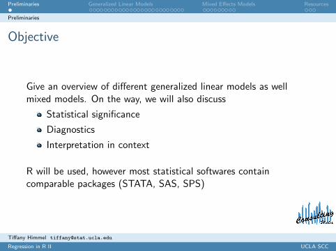
Objective
Give an overview of different generalized linear models as wellmixed models. On the way, we will also discuss
Statistical significance
Diagnostics
Interpretation in context
R will be used, however most statistical softwares containcomparable packages (STATA, SAS, SPS)
Tiffany Himmel [email protected]
Regression in R II UCLA SCC

Preliminaries Generalized Linear Models Mixed Effects Models Resources
1 Generalized Linear ModelsPoisson RegressionLogistic RegressionMultinomial Logistic
2 Mixed Effects Models
3 Resources
Tiffany Himmel [email protected]
Regression in R II UCLA SCC
Preliminaries Generalized Linear Models Mixed Effects Models Resources
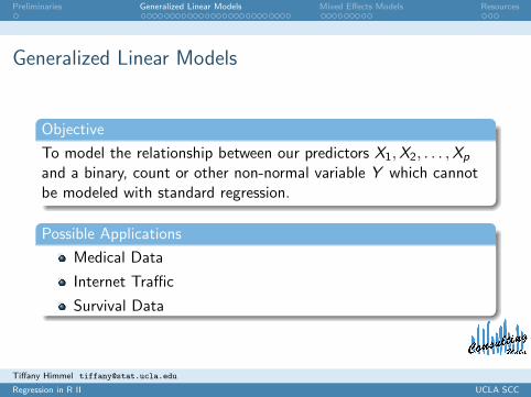
Generalized Linear Models
Objective
To model the relationship between our predictors X1,X2, . . . ,Xp
and a binary, count or other non-normal variable Y which cannotbe modeled with standard regression.
Possible Applications
Medical Data
Internet Traffic
Survival Data
Tiffany Himmel [email protected]
Regression in R II UCLA SCC
Preliminaries Generalized Linear Models Mixed Effects Models Resources
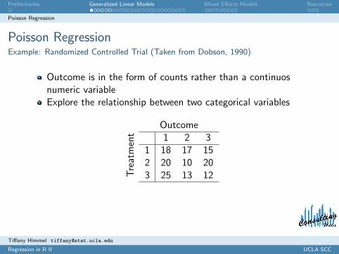
Poisson Regression
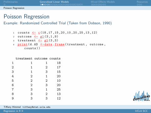
Poisson RegressionExample: Randomized Controlled Trial (Taken from Dobson, 1990)
Outcome is in the form of counts rather than a continuosnumeric variableExplore the relationship between two categorical variables
OutcomeT
reat
men
t 1 2 31 18 17 152 20 10 203 25 13 12
Tiffany Himmel [email protected]
Regression in R II UCLA SCC
Preliminaries Generalized Linear Models Mixed Effects Models Resources
Poisson Regression
Poisson RegressionExample: Randomized Controlled Trial (Taken from Dobson, 1990)
1 counts <- c(18 ,17 ,15 ,20 ,10 ,20 ,25 ,13 ,12)2 outcome <- gl(3,1,9)3 treatment <- gl(3,3)4 print(d.AD <-data.frame(treatment , outcome ,
counts))
treatment outcome counts1 1 1 182 1 2 173 1 3 154 2 1 205 2 2 106 2 3 207 3 1 258 3 2 139 3 3 12
Tiffany Himmel [email protected]
Regression in R II UCLA SCC

Preliminaries Generalized Linear Models Mixed Effects Models Resources
Poisson Regression
Exploratory PlotsExample: Randomized Controlled Trial (Taken from Dobson, 1990)
1 contin.table <-xtabs(counts~treatment+outcome)2 mosaicplot(contin.table ,main="Mosaic Plot")3 dimnames(contin.table)$outcome <-c("Out_1","Out
_2","Out_3")4 dimnames(contin.table)$treatment <-c("Treat_1",
"Treat_2","Treat_3")5 dotchart(contin.table ,main="Dot Chart")
Mosaic Plot
outcome
treatment
1 2 3
12
3
Treat_1
Treat_2
Treat_3
Treat_1
Treat_2
Treat_3
Treat_1
Treat_2
Treat_3
Out_1
Out_2
Out_3
10 15 20 25
Dot Chart
Tiffany Himmel [email protected]
Regression in R II UCLA SCC
Preliminaries Generalized Linear Models Mixed Effects Models Resources
Poisson Regression
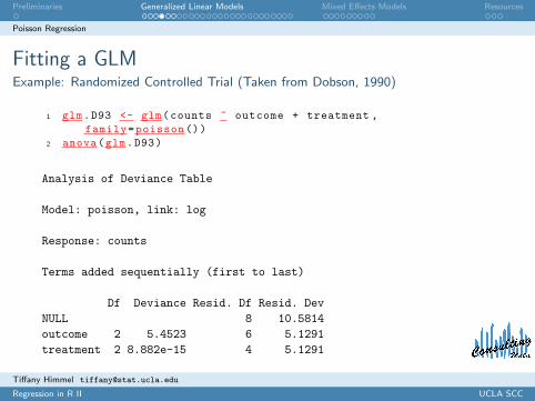
Fitting a GLMExample: Randomized Controlled Trial (Taken from Dobson, 1990)
1 glm.D93 <- glm(counts ~ outcome + treatment ,family=poisson ())
2 anova(glm.D93)
Analysis of Deviance Table
Model: poisson, link: log
Response: counts
Terms added sequentially (first to last)
Df Deviance Resid. Df Resid. DevNULL 8 10.5814outcome 2 5.4523 6 5.1291treatment 2 8.882e-15 4 5.1291
Tiffany Himmel [email protected]
Regression in R II UCLA SCC

Preliminaries Generalized Linear Models Mixed Effects Models Resources
Poisson Regression
Fitting a GLM IIExample: Randomized Controlled Trial (Taken from Dobson, 1990)
1 summary(glm.D93)
Coefficients:Estimate Std. Error z value Pr(>|z|)
(Intercept) 3.045e+00 1.709e-01 17.815 <2e-16 ***outcome2 -4.543e-01 2.022e-01 -2.247 0.0246 *outcome3 -2.930e-01 1.927e-01 -1.520 0.1285treatment2 1.338e-15 2.000e-01 6.69e-15 1.0000treatment3 1.421e-15 2.000e-01 7.11e-15 1.0000---Signif. codes: 0 *** 0.001 ** 0.01 * 0.05 . 0.1 1
(Dispersion parameter for poisson family taken to be 1)
Null deviance: 10.5814 on 8 degrees of freedomResidual deviance: 5.1291 on 4 degrees of freedomAIC: 56.761
Tiffany Himmel [email protected]
Regression in R II UCLA SCC
Preliminaries Generalized Linear Models Mixed Effects Models Resources
Poisson Regression
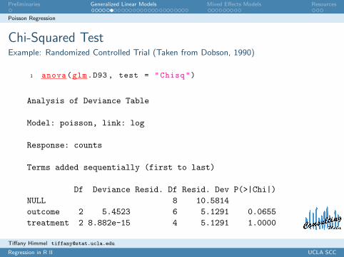
Chi-Squared TestExample: Randomized Controlled Trial (Taken from Dobson, 1990)
1 anova(glm.D93 , test = "Chisq")
Analysis of Deviance Table
Model: poisson, link: log
Response: counts
Terms added sequentially (first to last)
Df Deviance Resid. Df Resid. Dev P(>|Chi|)NULL 8 10.5814outcome 2 5.4523 6 5.1291 0.0655treatment 2 8.882e-15 4 5.1291 1.0000
Tiffany Himmel [email protected]
Regression in R II UCLA SCC

Preliminaries Generalized Linear Models Mixed Effects Models Resources
Logistic Regression
Logistic Regression
Like Poisson, outcomes are not continuousOutcome is in the form of binary variables
yes/no, dead/alive, male/femaleMakes estimates based on % yes/nox-covariate continuous (usually)
Very popular in medical research
Tiffany Himmel [email protected]
Regression in R II UCLA SCC
Preliminaries Generalized Linear Models Mixed Effects Models Resources
Logistic Regression
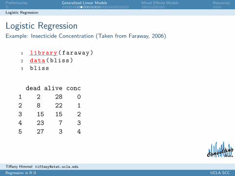
Logistic RegressionExample: Insecticide Concentration (Taken from Faraway, 2006)
1 library(faraway)2 data(bliss)3 bliss
dead alive conc1 2 28 02 8 22 13 15 15 24 23 7 35 27 3 4
Tiffany Himmel [email protected]
Regression in R II UCLA SCC

Preliminaries Generalized Linear Models Mixed Effects Models Resources
Logistic Regression
Exploratory PlotsExample: Insecticide Concentration (Taken from Faraway, 2006)
Thinking percentages...
1 attach(bliss)2 survival <-(alive/(alive+dead))3 bliss <-data.frame(bliss ,survival)4 plot(survival~conc ,main="Insecticide")
0 1 2 3 4
0.2
0.4
0.6
0.8
Insecticide
conc
survival
Tiffany Himmel [email protected]
Regression in R II UCLA SCC
Preliminaries Generalized Linear Models Mixed Effects Models Resources
Logistic Regression
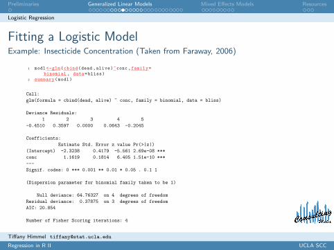
Fitting a Logistic ModelExample: Insecticide Concentration (Taken from Faraway, 2006)
1 modl <-glm(cbind(dead ,alive)~conc ,family=binomial , data=bliss)
2 summary(modl)
Call:glm(formula = cbind(dead, alive) ~ conc, family = binomial, data = bliss)
Deviance Residuals:1 2 3 4 5
-0.4510 0.3597 0.0000 0.0643 -0.2045
Coefficients:Estimate Std. Error z value Pr(>|z|)
(Intercept) -2.3238 0.4179 -5.561 2.69e-08 ***conc 1.1619 0.1814 6.405 1.51e-10 ***---Signif. codes: 0 *** 0.001 ** 0.01 * 0.05 . 0.1 1
(Dispersion parameter for binomial family taken to be 1)
Null deviance: 64.76327 on 4 degrees of freedomResidual deviance: 0.37875 on 3 degrees of freedomAIC: 20.854
Number of Fisher Scoring iterations: 4
Tiffany Himmel [email protected]
Regression in R II UCLA SCC

Preliminaries Generalized Linear Models Mixed Effects Models Resources
Logistic Regression
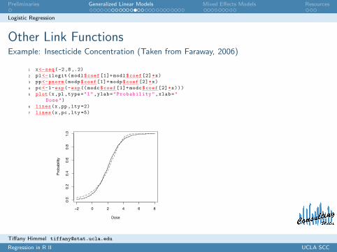
Other Link FunctionsExample: Insecticide Concentration (Taken from Faraway, 2006)
1 modp <-glm(cbind(dead ,alive)~conc ,family=binomial(link=probit),data=bliss)
2 modc <-glm(cbind(dead ,alive)~conc ,family=binomial(link=cloglog),data=bliss)
Tiffany Himmel [email protected]
Regression in R II UCLA SCC

Preliminaries Generalized Linear Models Mixed Effects Models Resources
Logistic Regression
Other Link FunctionsExample: Insecticide Concentration (Taken from Faraway, 2006)
1 cbind(fitted(modl),fitted(modp),fitted(modc))
[,1] [,2] [,3]1 0.08917177 0.08424186 0.12727002 0.23832314 0.24487335 0.24969093 0.50000000 0.49827210 0.45459104 0.76167686 0.75239612 0.72176555 0.91082823 0.91441122 0.9327715
Tiffany Himmel [email protected]
Regression in R II UCLA SCC
Preliminaries Generalized Linear Models Mixed Effects Models Resources
Logistic Regression
Other Link FunctionsExample: Insecticide Concentration (Taken from Faraway, 2006)
1 x<-seq(-2,8,.2)2 pl<-ilogit(modl$coef [1]+ modl$coef [2]*x)3 pp<-pnorm(modp$coef [1]+ modp$coef [2]*x)4 pc<-1-exp(-exp((modc$coef [1]+ modc$coef [2]*x)))5 plot(x,pl,type="l",ylab="Probability",xlab="
Dose")6 lines(x,pp ,lty=2)7 lines(x,pc ,lty=5)
Preliminaries Introduction Multivariate Linear Regression Advanced Resources References Upcoming Survey Questions
Binomial Regression
Other Link FunctionsExample: Insecticide Concentration (Taken from Faraway, 2006)
1 x<-seq(-2,8,.2)2 pl<-ilogit(modl$coef [1]+ modl$coef [2]*x)3 pp<-pnorm(modp$coef [1]+ modp$coef [2]*x)4 pc<-1-exp(-exp((modc$coef [1]+ modc$coef [2]*x)))5 plot(x,pl,type="l",ylab="Probability",xlab="
Dose")6 lines(x,pp ,lty=2)7 lines(x,pc ,lty=5)
−2 0 2 4 6 8
0.0
0.2
0.4
0.6
0.8
1.0
Dose
Probability
Denise Ferrari [email protected]
Regression in R I UCLA SCC
Tiffany Himmel [email protected]
Regression in R II UCLA SCC
Preliminaries Generalized Linear Models Mixed Effects Models Resources
Logistic Regression
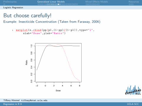
But choose carefully!Example: Insecticide Concentration (Taken from Faraway, 2006)
1 matplot(x,cbind(pp/pl ,(1-pp)/(1-pl)),type="l",xlab="Dose",ylab="Ratio")
Preliminaries Introduction Multivariate Linear Regression Advanced Resources References Upcoming Survey Questions
Binomial Regression
But choose carefully!Example: Insecticide Concentration (Taken from Faraway, 2006)
1 matplot(x,cbind(pp/pl ,(1-pp)/(1-pl)),type="l",xlab="Dose",ylab="Ratio")
−2 0 2 4 6 8
0.0
0.2
0.4
0.6
0.8
1.0
Dose
Ratio
Denise Ferrari [email protected]
Regression in R I UCLA SCC
Tiffany Himmel [email protected]
Regression in R II UCLA SCC

Preliminaries Generalized Linear Models Mixed Effects Models Resources
Logistic Regression
But choose carefully!Example: Insecticide Concentration (Taken from Faraway, 2006)
1 matplot(x,cbind(pc/pl ,(1-pc)/(1-pl)),type="l",xlab="Dose",ylab="Ratio")
Preliminaries Introduction Multivariate Linear Regression Advanced Resources References Upcoming Survey Questions
Binomial Regression
But choose carefully!Example: Insecticide Concentration (Taken from Faraway, 2006)
1 matplot(x,cbind(pc/pl ,(1-pc)/(1-pl)),type="l",xlab="Dose",ylab="Ratio")
−2 0 2 4 6 8
0.0
0.5
1.0
1.5
2.0
2.5
3.0
Dose
Ratio
Denise Ferrari [email protected]
Regression in R I UCLA SCC
Tiffany Himmel [email protected]
Regression in R II UCLA SCC
Preliminaries Generalized Linear Models Mixed Effects Models Resources
Multinomial Logistic
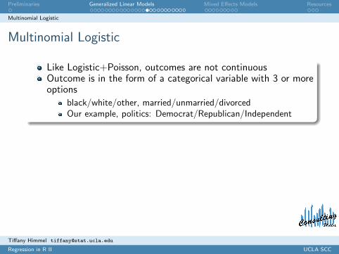
Multinomial Logistic
Like Logistic+Poisson, outcomes are not continuousOutcome is in the form of a categorical variable with 3 or moreoptions
black/white/other, married/unmarried/divorcedOur example, politics: Democrat/Republican/Independent
Tiffany Himmel [email protected]
Regression in R II UCLA SCC
Preliminaries Generalized Linear Models Mixed Effects Models Resources
Multinomial Logistic
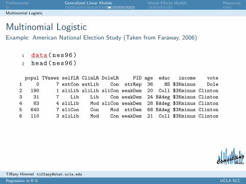
Multinomial LogisticExample: American National Election Study (Taken from Faraway, 2006)
1 data(nes96)2 head(nes96)
popul TVnews selfLR ClinLR DoleLR PID age educ income vote
1 0 7 extCon extLib Con strRep 36 HS $3Kminus Dole
2 190 1 sliLib sliLib sliCon weakDem 20 Coll $3Kminus Clinton
3 31 7 Lib Lib Con weakDem 24 BAdeg $3Kminus Clinton
4 83 4 sliLib Mod sliCon weakDem 28 BAdeg $3Kminus Clinton
5 640 7 sliCon Con Mod strDem 68 BAdeg $3Kminus Clinton
6 110 3 sliLib Mod Con weakDem 21 Coll $3Kminus Clinton
Tiffany Himmel [email protected]
Regression in R II UCLA SCC

Preliminaries Generalized Linear Models Mixed Effects Models Resources
Multinomial Logistic
Exploratory PlotsExample: American National Election Study (Taken from Faraway, 2006)
1 PartyAffil <-nes96$PID2 levels(PartyAffil)<-c("Dem","Dem","Ind","Ind",
"Ind","Rep","Rep")3 income.categories <-c(1.5, 4, 6, 8, 9., 10.5,
11.5, 12.5, 13.5, 14.5, 16, 18.5, 21, 23.5,27.5, 32.5, 37.5, 42.5, 47.5, 55, 67.5,
82.5, 97.5, 115)4 Income.numeric <-income.categories[unclass(
nes96$income)]5 hist(Income.numeric ,main="")
Income.numeric
Frequency
0 20 40 60 80 100 120
020
4060
80100
120
Tiffany Himmel [email protected]
Regression in R II UCLA SCC

Preliminaries Generalized Linear Models Mixed Effects Models Resources
Multinomial Logistic
Useful TablesExample: American National Election Study (Taken from Faraway, 2006)
1 Income.Split <-cut(Income.numeric ,7)2 PartyProp.by.Income <-prop.table(table(Income.
Split ,PartyAffil) ,1)
PartyAffilIncome.Split Dem Ind Rep
(1.39,17.6] 0.5402299 0.2356322 0.2241379(17.6,33.9] 0.5000000 0.1932773 0.3067227(33.9,50.1] 0.4409938 0.2236025 0.3354037(50.1,66.4] 0.2900000 0.3400000 0.3700000(66.4,82.6] 0.2820513 0.2628205 0.4551282(82.6,98.9] 0.1914894 0.3191489 0.4893617(98.9,115] 0.2058824 0.3823529 0.4117647
Tiffany Himmel [email protected]
Regression in R II UCLA SCC

Preliminaries Generalized Linear Models Mixed Effects Models Resources
Multinomial Logistic
Exploratory Plots IIExample: American National Election Study (Taken from Faraway, 2006)
1 Income.Split.Mids <-c(8 ,26 ,42 ,58 ,74 ,90 ,107)2 matplot(Income.Split.Mids ,PartyProp.by.Income ,
lty=c(1,2,3),col=c(5,3,4),lwd=2,type="l",xlab="Income in 10s of Thousands",ylab="Party Proportion by Income")
3 legend (45,.54,c("Democrat","Independent","Republican"),col=c(5,3,4),lty=c(1,2,3))
20 40 60 80 100
0.20
0.25
0.30
0.35
0.40
0.45
0.50
0.55
Income in 10s of Thousands
Par
ty P
ropo
rtion
by
Inco
me
DemocratIndependentRepublican
Tiffany Himmel [email protected]
Regression in R II UCLA SCC

Preliminaries Generalized Linear Models Mixed Effects Models Resources
Multinomial Logistic
Fitting a Multinomial Logistic ModelExample: American National Election Study (Taken from Faraway, 2006)
1 library(nnet)2 multinomial.model <-multinom(PartyAffil~Income.
numeric)3 summary(multinomial.model)
Coefficients:(Intercept) Income.numeric
Ind -1.173592 0.01606080Rep -0.949674 0.01765140
Std. Errors:(Intercept) Income.numeric
Ind 0.1535317 0.002848357Rep 0.1416261 0.002651135
Residual Deviance: 1985.485AIC: 1993.485
Tiffany Himmel [email protected]
Regression in R II UCLA SCC

Preliminaries Generalized Linear Models Mixed Effects Models Resources
Multinomial Logistic
Making PredictionsExample: American National Election Study (Taken from Faraway, 2006)
1 predict(multinomial.model ,data.frame(Income.numeric=Income.Split.Mids))
2 Party.Prob.Predictions <-predict(multinomial.model ,data.frame(Income.numeric=Income.Split.Mids),type="probs")
Dem Ind Rep1 0.5564220 0.1956684 0.24790962 0.4803742 0.2255528 0.29407303 0.4133828 0.2509706 0.33564674 0.3494149 0.2742923 0.37629285 0.2904121 0.2947737 0.41481426 0.2377033 0.3119688 0.45032787 0.1893241 0.3264816 0.4841943
Tiffany Himmel [email protected]
Regression in R II UCLA SCC
Preliminaries Generalized Linear Models Mixed Effects Models Resources
Multinomial Logistic
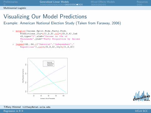
Visualizing Our Model PredictionsExample: American National Election Study (Taken from Faraway, 2006)
1 matplot(Income.Split.Mids ,Party.Prob.Predictions ,lty=c(1,2,3),col=c(5,3,4),lwd=2,type="l",xlab="Income in 10s ofThousands",ylab="Party Proportion by Income")
2 legend (45,.54,c("Democrat","Independent","Republican"),col=c(5,3,4),lty=c(1,2,3))
20 40 60 80 100
0.2
0.3
0.4
0.5
Income in 10s of Thousands
Par
ty P
ropo
rtion
by
Inco
me
DemocratIndependentRepublican
Tiffany Himmel [email protected]
Regression in R II UCLA SCC
Preliminaries Generalized Linear Models Mixed Effects Models Resources
Multinomial Logistic
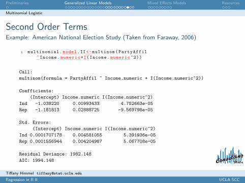
Second Order TermsExample: American National Election Study (Taken from Faraway, 2006)
1 multinomial.model.II<-multinom(PartyAffil~Income.numeric+I(Income.numeric ^2))
Call:multinom(formula = PartyAffil ~ Income.numeric + I(Income.numeric^2))
Coefficients:(Intercept) Income.numeric I(Income.numeric^2)
Ind -1.038220 0.00993433 4.752663e-05Rep -1.181813 0.02888725 -9.569798e-05
Std. Errors:(Intercept) Income.numeric I(Income.numeric^2)
Ind 0.0001707178 0.004581055 5.391936e-05Rep 0.0001556944 0.004204987 5.067708e-05
Residual Deviance: 1982.148AIC: 1994.148
Tiffany Himmel [email protected]
Regression in R II UCLA SCC

Preliminaries Generalized Linear Models Mixed Effects Models Resources
Multinomial Logistic
Visualizing Our Model Predictions IIExample: American National Election Study (Taken from Faraway, 2006)
1 predict(multinomial.model.II ,data.frame(Income.numeric=Income.Split.Mids))
2 Party.Prob.Predictions.II<-predict(multinomial.model.II, data.frame(Income.numeric=Income.Split.Mids), type="probs")
3 matplot(Income.Split.Mids ,Party.Prob.Predictions.II,lty=c(1,2,3),col=c(5,3,4),lwd=2,type="l",xlab="Income in 10s ofThousands",ylab="Party Proportion by Income")
4 legend (45,.54,c("Democrat","Independent","Republican"),col=c(5,3,4),lty=c(1,2,3))
20 40 60 80 100
0.2
0.3
0.4
0.5
Income in 10s of Thousands
Par
ty P
ropo
rtion
by
Inco
me
DemocratIndependentRepublican
Tiffany Himmel [email protected]
Regression in R II UCLA SCC
Preliminaries Generalized Linear Models Mixed Effects Models Resources
Multinomial Logistic
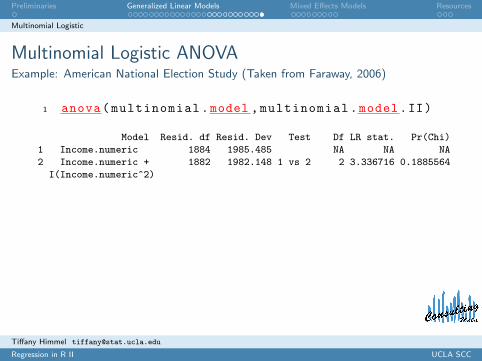
Multinomial Logistic ANOVAExample: American National Election Study (Taken from Faraway, 2006)
1 anova(multinomial.model ,multinomial.model.II)
Model Resid. df Resid. Dev Test Df LR stat. Pr(Chi)
1 Income.numeric 1884 1985.485 NA NA NA
2 Income.numeric + 1882 1982.148 1 vs 2 2 3.336716 0.1885564
I(Income.numeric^2)
Tiffany Himmel [email protected]
Regression in R II UCLA SCC

Preliminaries Generalized Linear Models Mixed Effects Models Resources
1 Generalized Linear Models
2 Mixed Effects ModelsDefinitionsModel FittingAssumption Validation
3 Resources
Tiffany Himmel [email protected]
Regression in R II UCLA SCC

Preliminaries Generalized Linear Models Mixed Effects Models Resources
Definitions
What is a Mixed Effects Model?
Fixed effect: β is the same over all groups/patients
Random Effect: νi ∼ N(0, σ2ν) where each group has their
own coefficient
Often used in medical or survey data
yij = β0 + . . .+ βl︸ ︷︷ ︸fixed effects
+ ν1i + . . .+ νmi︸ ︷︷ ︸random effects
+ εij︸︷︷︸residual
subject i = 1 . . . n← # of subjectsobservation j = 1 . . . ni ← # of observations for that subject
Tiffany Himmel [email protected]
Regression in R II UCLA SCC

Preliminaries Generalized Linear Models Mixed Effects Models Resources
Model Fitting
Exploratory PlotsExample: Sleep Study (Taken from Belenky et al., 2003)
1 library(lme4)2 data(sleepstudy)3 xyplot(Reaction ~ Days | Subject , sleepstudy ,
type = c("g","p","r"),index = function(x,y)coef(lm(y ~ x))[1], xlab = "Days of sleep
deprivation", ylab = "Average reaction time(ms)", aspect = "xy")
Days of sleep deprivation
Ave
rage
reac
tion
time
(ms)
200
250
300
350
400
450
0 2 4 6 8
310 309
0 2 4 6 8
370 349
0 2 4 6 8
350 334
308 371 369 351 335
200
250
300
350
400
450
332200
250
300
350
400
450
372
0 2 4 6 8
333 352
0 2 4 6 8
331 330
0 2 4 6 8
337
Tiffany Himmel [email protected]
Regression in R II UCLA SCC

Preliminaries Generalized Linear Models Mixed Effects Models Resources
Model Fitting
Fitting a Mixed Effects ModelExample: Sleep Study (Taken from Belenky et al., 2003)
1 (fm1 <- lmer(Reaction ~ Days + (Days|Subject),sleepstudy))
AIC BIC logLik deviance REMLdev1756 1775 -871.8 1752 1744
Random effects:Groups Name Variance Std.Dev. CorrSubject (Intercept) 612.092 24.7405
Days 35.072 5.9221 0.066Residual 654.941 25.5918
Number of obs: 180, groups: Subject, 18
Fixed effects:Estimate Std. Error t value
(Intercept) 251.405 6.825 36.84Days 10.467 1.546 6.77
Correlation of Fixed Effects:(Intr)
Days -0.138
Tiffany Himmel [email protected]
Regression in R II UCLA SCC

Preliminaries Generalized Linear Models Mixed Effects Models Resources
Model Fitting
Fitting a Mixed Effects Model IIExample: Sleep Study (Taken from Belenky et al., 2003)
1 (fm2 <- lmer(Reaction ~ Days + (1| Subject) +(0+ Days|Subject), sleepstudy))
AIC BIC logLik deviance REMLdev1754 1770 -871.8 1752 1744
Random effects:Groups Name Variance Std.Dev.Subject (Intercept) 627.568 25.0513Subject Days 35.858 5.9882Residual 653.584 25.5653
Number of obs: 180, groups: Subject, 18
Fixed effects:Estimate Std. Error t value
(Intercept) 251.405 6.885 36.51Days 10.467 1.559 6.71
Correlation of Fixed Effects:(Intr)
Days -0.184
Tiffany Himmel [email protected]
Regression in R II UCLA SCC
Preliminaries Generalized Linear Models Mixed Effects Models Resources
Model Fitting
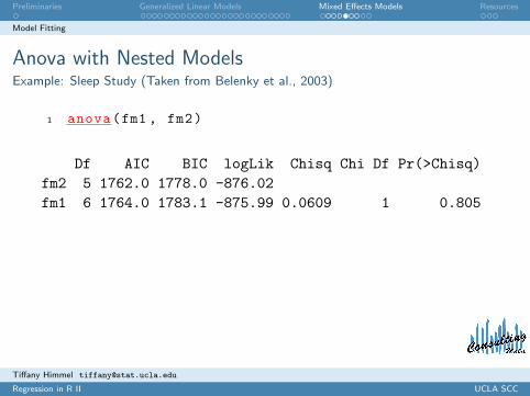
Anova with Nested ModelsExample: Sleep Study (Taken from Belenky et al., 2003)
1 anova(fm1 , fm2)
Df AIC BIC logLik Chisq Chi Df Pr(>Chisq)fm2 5 1762.0 1778.0 -876.02fm1 6 1764.0 1783.1 -875.99 0.0609 1 0.805
Tiffany Himmel [email protected]
Regression in R II UCLA SCC
Preliminaries Generalized Linear Models Mixed Effects Models Resources
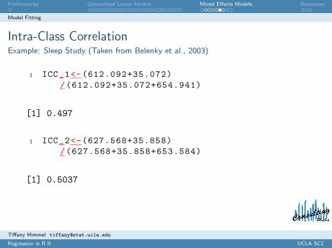
Model Fitting
Intra-Class CorrelationExample: Sleep Study (Taken from Belenky et al., 2003)
1 ICC_1<-(612.092+35.072)/(612.092+35.072+654.941)
[1] 0.497
1 ICC_2<-(627.568+35.858)/(627.568+35.858+653.584)
[1] 0.5037
Tiffany Himmel [email protected]
Regression in R II UCLA SCC
Preliminaries Generalized Linear Models Mixed Effects Models Resources
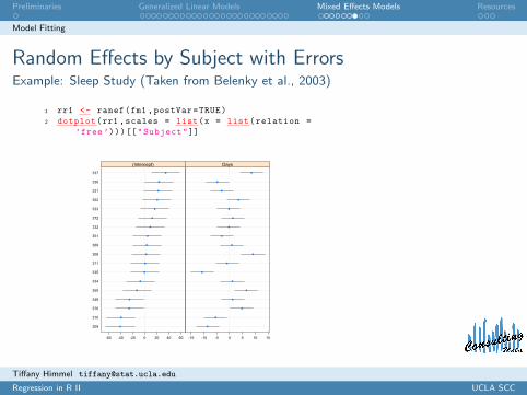
Model Fitting
Random Effects by Subject with ErrorsExample: Sleep Study (Taken from Belenky et al., 2003)
1 rr1 <- ranef(fm1 ,postVar=TRUE)2 dotplot(rr1 ,scales = list(x = list(relation =
’free’)))[["Subject"]]
309
310
370
349
350
334
335
371
308
369
351
332
372
333
352
331
330
337
-60 -40 -20 0 20 40 60
(Intercept)
-15 -10 -5 0 5 10 15
Days
Tiffany Himmel [email protected]
Regression in R II UCLA SCC
Preliminaries Generalized Linear Models Mixed Effects Models Resources
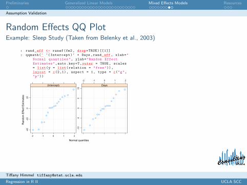
Assumption Validation
Random Effects QQ PlotExample: Sleep Study (Taken from Belenky et al., 2003)
1 rand_eff <- ranef(fm2 , drop=TRUE)[[1]]2 qqmath(~ ‘(Intercept)‘ + Days ,rand_eff , xlab="
Normal quantiles", ylab="Random EffectEstimates",auto.key=T,outer = TRUE , scales= list(y = list(relation = "free")),layout = c(2,1), aspect = 1, type = c("g","p"))
Normal quantiles
Ran
dom
Effe
ct E
stim
ates
-40
-20
020
-2 -1 0 1 2
(Intercept)
-2 -1 0 1 2-10
-50
510
Days
Tiffany Himmel [email protected]
Regression in R II UCLA SCC
Preliminaries Generalized Linear Models Mixed Effects Models Resources
Assumption Validation
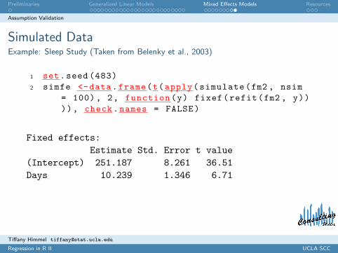
Simulated DataExample: Sleep Study (Taken from Belenky et al., 2003)
1 set.seed (483)2 simfe <-data.frame(t(apply(simulate(fm2 , nsim
= 100), 2, function(y) fixef(refit(fm2 , y)))), check.names = FALSE)
Fixed effects:Estimate Std. Error t value
(Intercept) 251.187 8.261 36.51Days 10.239 1.346 6.71
Tiffany Himmel [email protected]
Regression in R II UCLA SCC

Preliminaries Generalized Linear Models Mixed Effects Models Resources
1 Generalized Linear Models
2 Mixed Effects Models
3 ResourcesOnline Resources for RReferences
Tiffany Himmel [email protected]
Regression in R II UCLA SCC
Preliminaries Generalized Linear Models Mixed Effects Models Resources
Online Resources for R
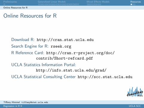
Online Resources for R
Download R: http://cran.stat.ucla.edu
Search Engine for R: rseek.org
R Reference Card: http://cran.r-project.org/doc/contrib/Short-refcard.pdf
UCLA Statistics Information Portal:http://info.stat.ucla.edu/grad/
UCLA Statistical Consulting Center http://scc.stat.ucla.edu
Tiffany Himmel [email protected]
Regression in R II UCLA SCC

Preliminaries Generalized Linear Models Mixed Effects Models Resources
References
References I
P. DaalgardIntroductory Statistics with R,Statistics and Computing, Springer-Verlag, NY, 2002.
B.S. Everitt and T. HothornA Handbook of Statistical Analysis using R,Chapman & Hall/CRC, 2006.
J.J. FarawayPractical Regression and Anova using R,www.stat.lsa.umich.edu/~faraway/book
Tiffany Himmel [email protected]
Regression in R II UCLA SCC

Preliminaries Generalized Linear Models Mixed Effects Models Resources
References
References II
J. Maindonald and J. BraunData Analysis and Graphics using R – An Example-BasedApproach,Second Edition, Cambridge University Press, 2007.
[Sheather, 2009] S.J. SheatherA Modern Approach to Regression with R,DOI: 10.1007/978-0-387-09608-7-3,Springer Science + Business Media LCC 2009.
Tiffany Himmel [email protected]
Regression in R II UCLA SCC