advanced spatial analysis - christina friedle
TRANSCRIPT

ADVANCED SPATIAL ANALYSIS
GIS Analysis | Fall 2013

There are many types of Spatial Analysis (Vector &
Raster). This lecture is focused on the following types
of Advanced Analysis:
Spatial Descriptive Statistics
Spatial Interpolation
Image Classification
Surface Analysis
Optimization
1st Law of Geography
Waldo Tober’s 1st Law of Geography
"Everything is related to everything else, but near things
are more related than distant things.”
Spatial Autocorrelation
A measure of the degree to which a set of spatial
features and their associated data values tend to be
clustered together in space (positive spatial
correlation) or dispersed (negative spatial
autocorrelation)

Spatial Descriptive Statistics

Spatial Descriptive Statistics
Spatial equivalent of the descriptive statistics
commonly used in statistical analysis, e.g. mean and
standard deviation.
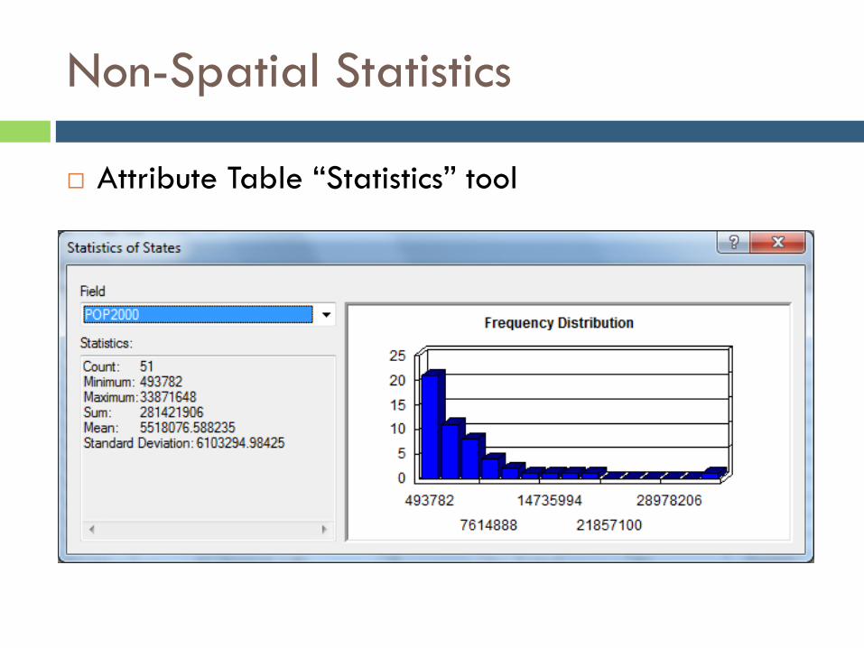
Non-Spatial Statistics
Attribute Table “Statistics” tool
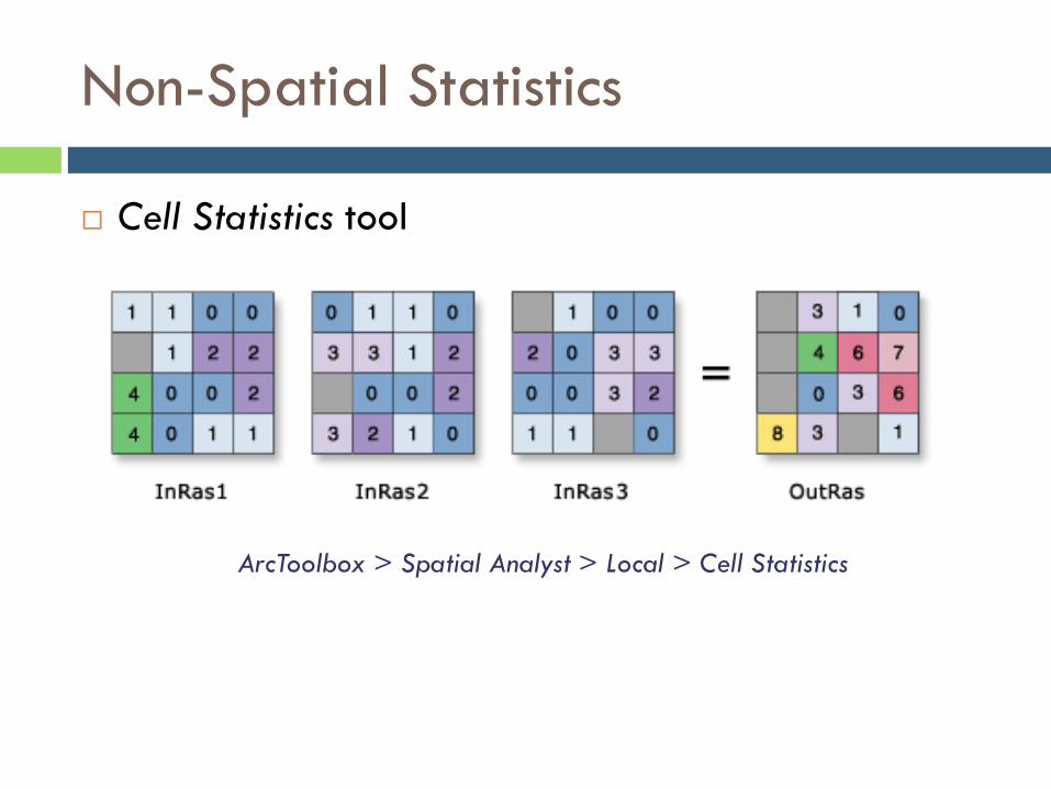
Non-Spatial Statistics
Cell Statistics tool
ArcToolbox > Spatial Analyst > Local > Cell Statistics

Common Spatial Descriptive Statistics
Nearest Neighbor index
Spatial Autocorrelation (Moran’s I)
Mean Center
K-means algorithm
Thiessen (Voronoi) polygons
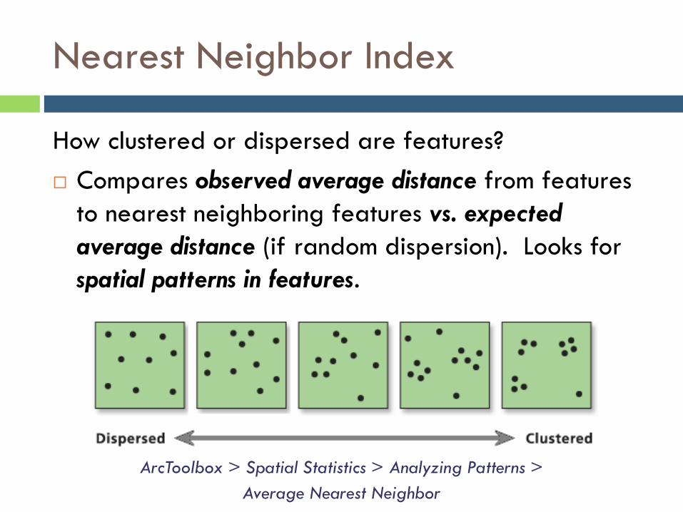
Nearest Neighbor Index
How clustered or dispersed are features?
Compares observed average distance from features
to nearest neighboring features vs. expected
average distance (if random dispersion). Looks for
spatial patterns in features.
ArcToolbox > Spatial Statistics > Analyzing Patterns >
Average Nearest Neighbor

Nearest Neighbor Index
Output of Nearest Neighbor Index is an index value
and related statistics; can be viewed in the
Geoprocessing “Results” window, or used in analysis
models/scripts.

Nearest Neighbor Index

Spatial Autocorrelation Index (Moran’s I)
Measures the similarity among feature attributes
relative to feature locations. Looks for spatial patterns
in attributes.
ArcToolbox > Spatial Statistics > Analyzing Patterns > Spatial Autocorrelation
(Morans I)
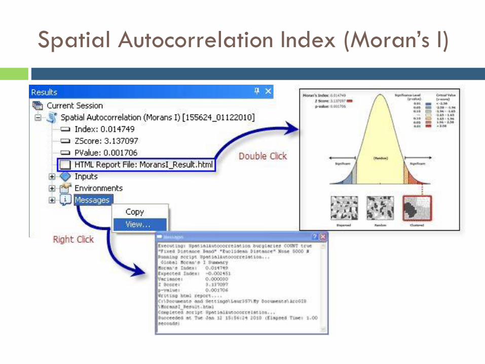
Spatial Autocorrelation Index (Moran’s I)
Output of Spatial Autocorrelation is also an index
value and related statistics accessed via “Results”
window.
Spatial Autocorrelation Index (Moran’s I)
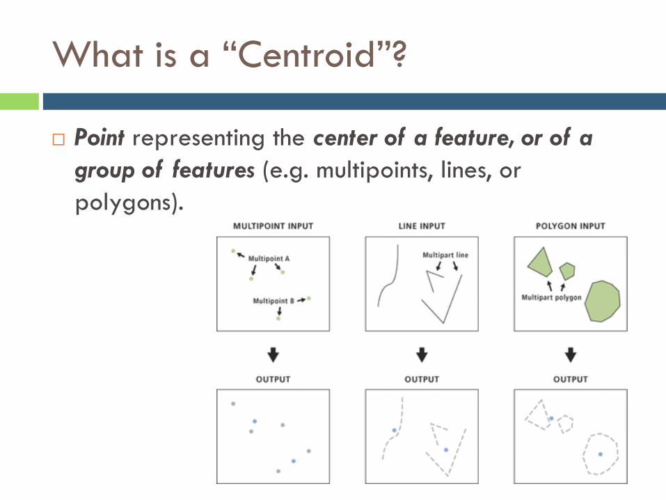
What is a “Centroid”?
Point representing the center of a feature, or of a
group of features (e.g. multipoints, lines, or
polygons).

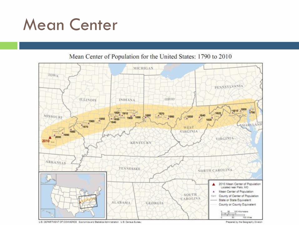
Mean Center
Average of all input points or centroids (based on
x/y values). Output is a single point.
ArcToolbox > Spatial Statistics >
Measuring Geographic Distributions > Mean Center
Mean Center

K-means
An iterative (repeating) algorithm that finds
geographic groups of point features and determines
their mean centers (e.g. store locations). Output is a
set of points.

Thiessen (Voronoi) Polygons
Each thiessen polygon contains a single point. Any
location within a polygon is closer to its associated
point than any other point feature (e.g. store
coverage areas). Output is a set of polygons.
ArcToolbox > Analysis > Proximity > Create Thiessen Polygons
Spatial Interpolation
Spatial Interpolation
Estimating values of a continuous representation in
places where the values have not been measured
In ArcGIS, spatial interpolation tools generate a
new raster dataset
Spatial Interpolation Methods
Spline
Inverse-distance weighting (IDW)
Kriging
Density Estimation
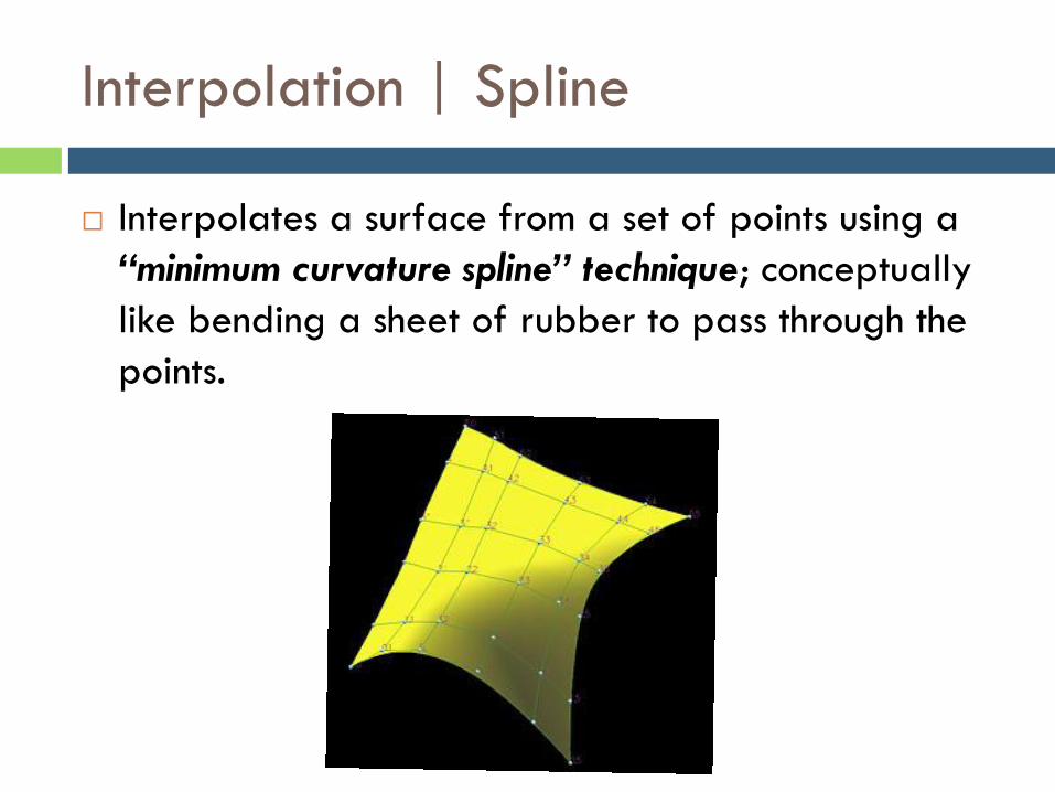
Interpolation | Spline
Interpolates a surface from a set of points using a
“minimum curvature spline” technique; conceptually
like bending a sheet of rubber to pass through the
points.

Interpolation | Inverse-distance weighting (IDW)
Estimates unknown values as weighted averages of
the known measurements at nearby points, giving
the greatest weight to the nearest points (using
Tobler’s Law).

Interpolation | Kriging
Similar to the IDW method in that it applies weights
to the data based on distance;
Differs from IDW in that it also takes into account
the form and spatial structure of all the data.
Provides a measure of the
certainty or accuracy of the
prediction.
Best used when data is known
to have spatial autocorrelation

Inverse Distance Weighting (IDW) Kriging
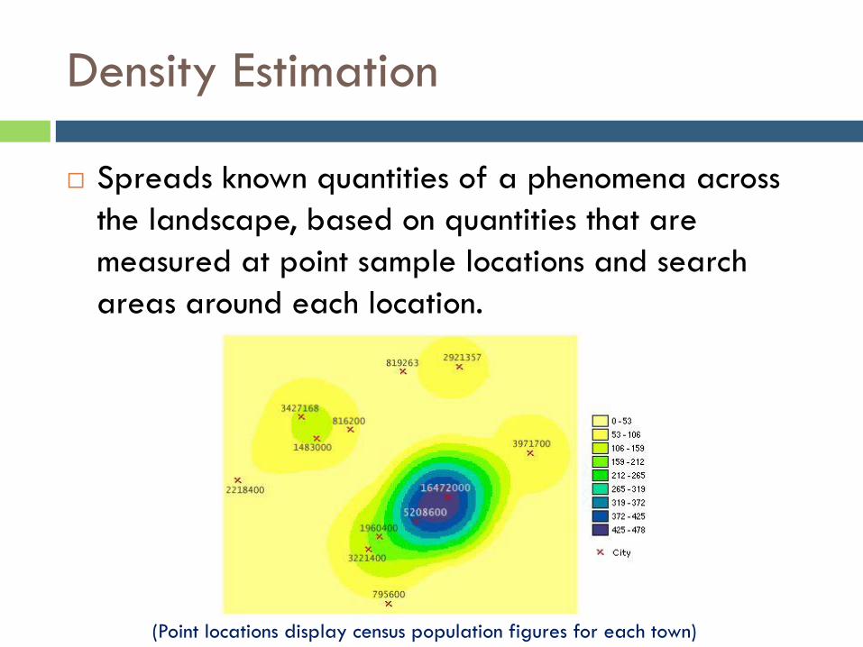
Density Estimation
Spreads known quantities of a phenomena across
the landscape, based on quantities that are
measured at point sample locations and search
areas around each location.
(Point locations display census population figures for each town)

Population Density across USA

Image Classification

Image Classification
Extracts information from a multi-band raster image

Image Classification | Unsupervised
Finds natural groupings (clusters) of spectral classes
in a multi-band image; e.g. Island vs. Ocean
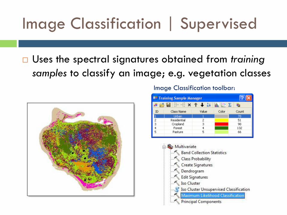
Image Classification | Supervised
Uses the spectral signatures obtained from training
samples to classify an image; e.g. vegetation classes
Image Classification toolbar:

Surface Analysis

Surface Analysis based on Elevation
Operations related to analysis of raster surfaces
Variety available in ArcToolbox:
Slope
Hillshade
Aspect
Contours
Viewshed
Watershed delineation

Slope
The incline or steepness of a surface or terrain
Can be measured in degrees (0-90) or percent
slope (rise/run)*100

Hillshade
Shadows drawn on a map to simulate the effect of
the sun’s rays over the varied terrain of the land
Creates a 3D effect that provides a visual sense of
shaded relief and a relative measure of incident
height for analysis


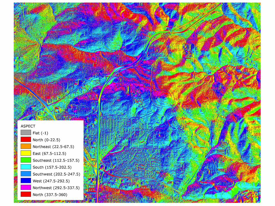
Aspect
The compass direction that a topographic slope
faces, usually measured in degrees from North
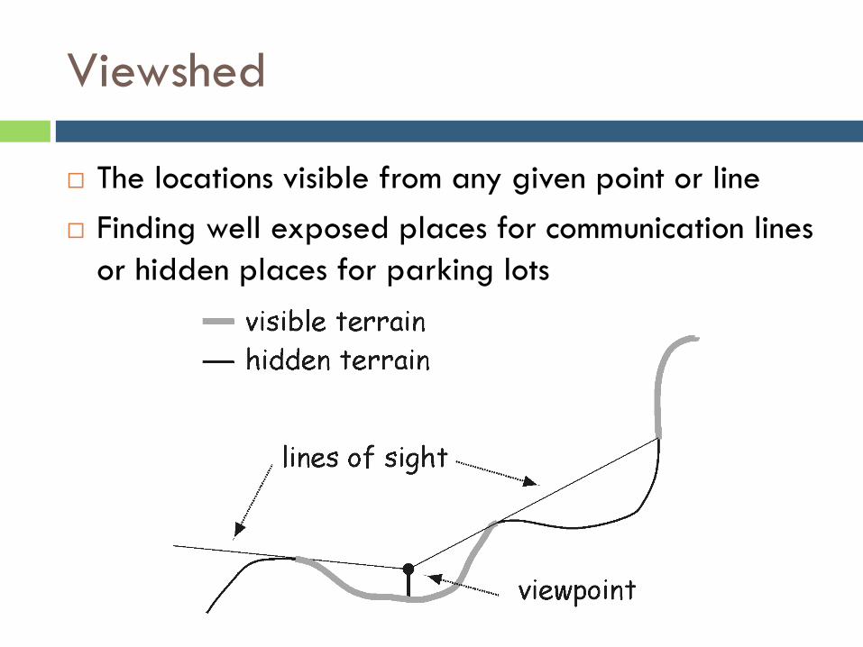
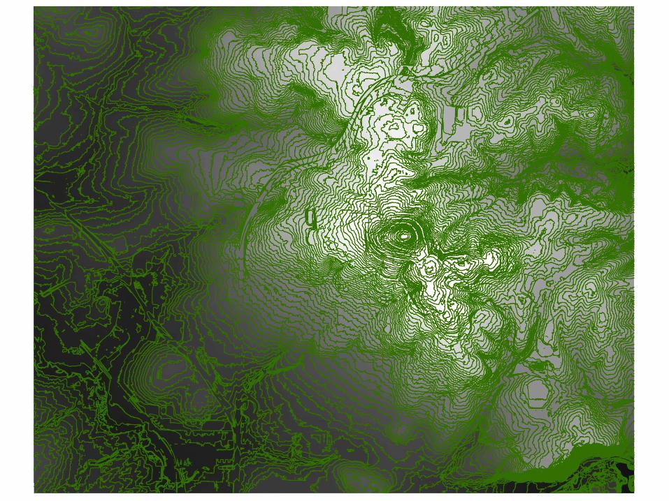
Viewshed
The locations visible from any given point or line
Finding well exposed places for communication lines
or hidden places for parking lots

Elevation in the area of the observation point
Green cells are visible from the observation point
Viewshed

Contour Lines
A line on a map that connects points of equal
elevation usually based on sea level (or another
vertical datum)
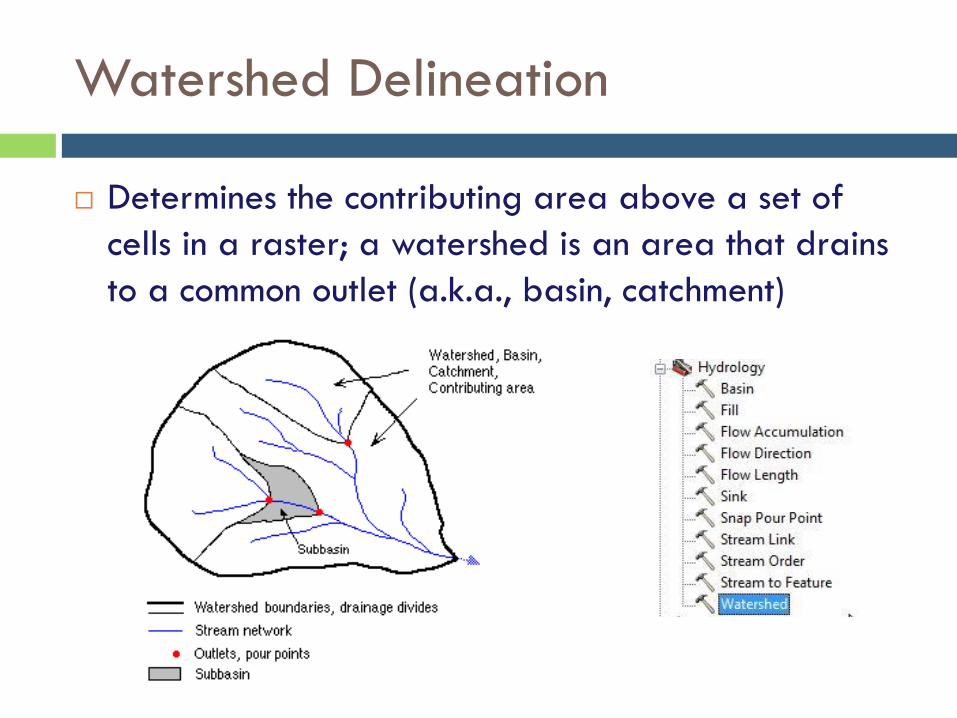
Watershed Delineation
Determines the contributing area above a set of
cells in a raster; a watershed is an area that drains
to a common outlet (a.k.a., basin, catchment)

Optimization

Optimization
Analytical techniques used to determine the best
(optimal) path, location, or other geographic
parameter based on a set of criteria
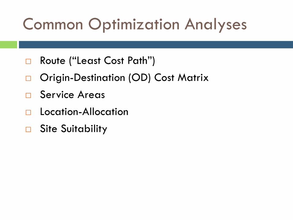
Common Optimization Analyses
Route (“Least Cost Path”)
Origin-Destination (OD) Cost Matrix
Service Areas
Location-Allocation
Site Suitability

Route (“Least Cost Path”) Analysis
Computes a travel route between locations along a
network, based on impedance (e.g. distance, time,
scenic beauty).
The “best” path is the one with the lowest impedance
score, or “least cost”.
Network Analyst toolbar > New Route

Origin-Destination (OD) Cost Matrix Analysis
Finds and measures distances along network least-
cost paths, from multiple origins to multiple
destinations
Network Analyst toolbar > New OD (Origin-Destination) Cost Matrix (layer)

Service Areas Analysis
Identifies areas along all paths in a network that are
within an impedance value (e.g. 5 minutes) from a
starting location.
Network Analyst toolbar > New Service Area (layer)

Location-Allocation Analysis
Locates facilities in such a way that demand for
services is allocated to each facility efficiently.
Network Analyst toolbar > New Location-Allocation (layer)
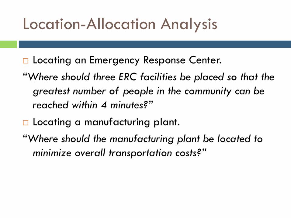
Location-Allocation Analysis
Locating an Emergency Response Center.
“Where should three ERC facilities be placed so that the
greatest number of people in the community can be
reached within 4 minutes?”
Locating a manufacturing plant.
“Where should the manufacturing plant be located to
minimize overall transportation costs?”
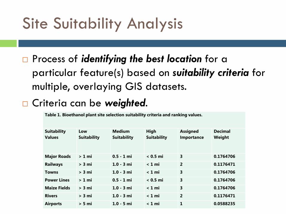
Site Suitability Analysis
Process of identifying the best location for a
particular feature(s) based on suitability criteria for
multiple, overlaying GIS datasets.
Criteria can be weighted.
Table 1. Bioethanol plant site selection suitability criteria and ranking values.
Suitability
Values
Low
Suitability
Medium
Suitability
High
Suitability
Assigned
Importance
Decimal
Weight
Major Roads > 1 mi 0.5 - 1 mi < 0.5 mi 3 0.1764706
Railways > 3 mi 1.0 - 3 mi < 1 mi 2 0.1176471
Towns > 3 mi 1.0 - 3 mi < 1 mi 3 0.1764706
Power Lines > 1 mi 0.5 - 1 mi < 0.5 mi 3 0.1764706
Maize Fields > 3 mi 1.0 - 3 mi < 1 mi 3 0.1764706
Rivers > 3 mi 1.0 - 3 mi < 1 mi 2 0.1176471
Airports > 5 mi 1.0 - 5 mi < 1 mi 1 0.0588235
