advanced statistical methods for observational studiesrogosateaching.com/somgen290/lect05.pdf ·...

L E C T U R E 0 5

Advanced Statistical Methods for Observational Studies

a small but important point

METRICS: Blinded Data Analysis as a Possible Antidote to

Confirmation Bias and P-hacking

Presented by: Robert MacCoun, PhD

Professor of Law Stanford University

To attend RSVP online by April 28, 2016

Monday, May 2, 2016 12:00-1:00 pm PST Li Ka Shing Center—LK209 Lunch will be served

http://goo.gl/forms/dqAYjh9uip

an example

Design of Observational Studies: chapter 5ish

matching on more than one metric

Intuition: matching on just propensity scores is like uniform randomization, whereas a Mahalanobis & pscores is more like a matched pairs randomization.

example

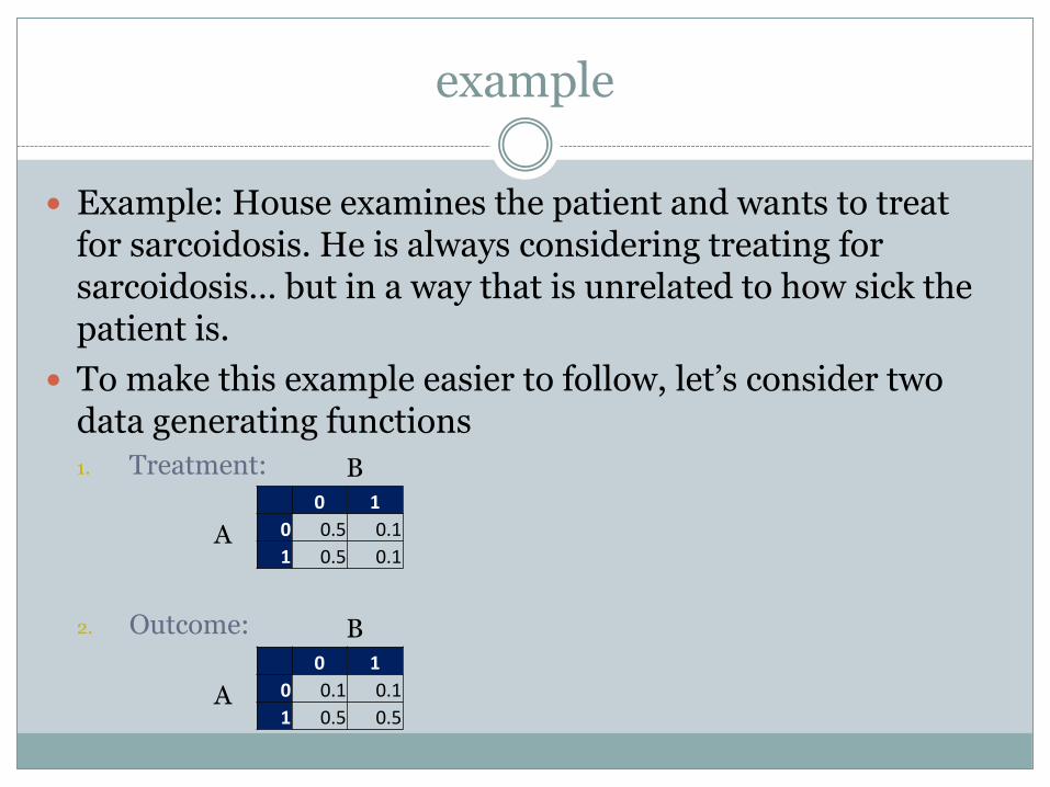
Example: House examines the patient and wants to treat for sarcoidosis. He is always considering treating for sarcoidosis… but in a way that is unrelated to how sick the patient is.

To make this example easier to follow, let’s consider two data generating functions 1. Treatment:

2. Outcome:

0 1

0 0.5 0.1

1 0.5 0.1 A

B

0 1

0 0.1 0.1

1 0.5 0.5 A

B

propensity score vs. prognostic score

This departure arises when the variables predictive of treatment differs from the prognostically relevant variables

This insight led to an interesting paper: Bhattacharya & Vogt “Do Instrumental Variables Belong in Propensity Scores?”

Prognostic score is one way to address this: Ben Hansen “The prognostic analog of the propensity score”

http://www.nber.org/papers/t0343

http://biomet.oxfordjournals.org/content/95/2/481.short

takeaway

This toy example highlights that the propensity score focuses on treatment, which may be unrelated to outcomes.

This is OK – the theory of inference is predicated on randomization, not identical units going into the groups (Fisher)

But it is better to start wish similar groups (Mill)

Next is an example of matching using both

matching on more than just the pscore

Example: We collected data on 251 people who reported for job training in the Bay Area. 131 smoked and 120 did not. We collected 20ish variables at baseline. We then looked at employment at 12 months.

Using a subset (30 smokers and 90 nonsmokers) let’s consider matching one treated to one control.

the smoking and employment example

Data set, first 4 smokers and 4 controls

smoker age

education years

bmi log(time

unemployed) Kessler score

gender white employed at 12 months

1 45 14 23.73167 5.192957 13 1 1 0

1 61 16 31.32101 3.401197 0 0 1 0

1 37 12 28.18891 5.347108 3 1 0 1

1 61 13 26.2897 5.010635 0 1 0 0

…

0 57 8 21.9247 8.202482 5 1 1 0

0 33 12 24.40488 7.286192 9 1 0 0

0 54 12 24.32526 8.202482 8 1 2 0

0 26 13 25.83983 5.192957 3 1 1 1


Table 1: pre-matching

variables mean

treated mean

control standardized

difference

smoker 1.00 0.00 2.30

age 47.53 46.21 0.12

education in years 14.80 13.12 0.64

bmi 27.48 26.48 0.17

log(time unemployed) 4.93 5.88 -0.64

Kessler score 5.87 7.06 -0.23

gender 0.37 0.78 -0.87

employed at 12 months 0.47 0.28 0.40


Table 1: matching on only pscore

variables mean

treated mean

control standardized

difference

smoker 1.00 0.00 2.30

age 47.53 45.93 0.14

education in years 14.80 14.43 0.14

bmi 27.48 28.01 -0.09

log(time unemployed) 4.93 5.24 -0.21

Kessler score 5.87 6.20 -0.06

gender 0.37 0.50 -0.28

employed at 12 months 0.47 0.23 0.50


1

2

3

4

5 6 7 8

difference: 𝑒 𝒙𝑖 − 𝑒 (𝒙𝑗)

-0.03 0.00 0.01 -0.03

-0.14 -0.11 -0.05 -0.14

0.00 0.04 0.04 0.00

-0.05 -0.01 0.00 -0.04

Design matrix (showing only 4 smokers and 4 nonsmokers)

d_temp <- read.csv("smoke_job.csv",header=TRUE)

mhd <- match_on(smoker ~ age+edu+bmi+

log_unemployed+kessler_score+gender

,data = d_temp)

ppty <- glm(smoker ~ age+edu+bmi+


,family = binomial()

,data = d_temp)

distmat <- match_on(ppty)

pm1 <- fullmatch(distmat,

min.controls=1,

max.controls = 1,

data = d_temp)

summary(pm1)

1:1 pscore matching


1

2

3

4

5 6 7 8

difference: 𝑒 𝒙𝑖 − 𝑒 (𝒙𝑗)

-0.03 0.00 0.01 -0.03

-0.14 -0.11 -0.05 -0.14

0.00 0.04 0.04 0.00

-0.05 -0.01 0.00 -0.04





,data = d_temp)




,data = d_temp)

distmat <- match_on(ppty)


min.controls=1,

max.controls = 4,

data = d_temp)

summary(pm1)

1:k variable pscore matching


1

2

3

4

5 6 7 8

0.37 0.16 0.31 1.12

0.88 0.68 0.62 1.16

0.00 0.27 0.26 0.80

0.28 0.13 0.04 0.88





,data = d_temp)




,data = d_temp)

distmat <- mhd


min.controls=1,

max.controls = 1,

data = d_temp)

summary(pm1)

1:1 MHD matching Mahalanobis distance


1

2

3

4

5 6 7 8

0.37 0.16 0.31 1.12

∞ ∞ 0.62 ∞

0.00 0.27 0.26 0.80

0.28 0.13 0.04 0.88


d_temp <- d[c(samp_smokers,samp_nonsmokers),]

mhd <- match_on(new_SC_CigPY ~ SC_Age+Educ_yrs_rec+BMIcalc+

logTimeUnempDayscut+logKesslerScore+

new_Gender+new_Race3level

,data = d_temp)

ppty <- glm(new_SC_CigPY ~ SC_Age+Educ_yrs_rec+BMIcalc+

logTimeUnempDayscut+logKesslerScore+

new_Gender+new_Race3level


,data = d_temp)

distmat <- mhd + caliper(match_on(ppty), width=0.10)


min.controls=1,

max.controls = 1,

data = d_temp)

summary(pm1)

1:1 MHD matching, with pscore caliper combined distance


How to retrieve matched set information

#post-matching

##pull the matched sets out of fullmatch

##i reduce the dataframe to just be the matched observations, this is not necessary

m1 <- names(matched(pm1))[matched(pm1)]

d_matched <- d[m1,]

#store set membership

pm1_sets <- paste("pm1.",sep="",pm1[matched(pm1)])

d_matched <- cbind(d_matched,pm1_sets)

#create a column to store number of controls so you can weight appropriately

set_size <- matrix(NA,nrow=length(pm1_sets),ncol=1)

for(i in 1:length(pm1_sets)){

set_size[i,] <- table(pm1_sets)[which(names(table(pm1_sets))==pm1_sets[i])]

}

d_matched <- cbind(d_matched,set_size)

See code posted on course website for more info on producing “Table 1” and overlapping histograms.


Non-overlap Look at a histogram

0.0 1.0 0.5

P(non-S|X) = Probability of being a non-smoker, given covariates



Upper and lower

0.0 1.0 0.5


Smokers only

Non-smokers

only



Upper and lower

Violation of strongly ignorable treatment assignment

Careful, need to consider what effect you’re estimating

What’s actually estimable and what isn’t

0.0 1.0 0.5


Smokers only

Non-smokers

only

the observations we can use in our study.



Upper and lower

Violation of strongly ignorable treatment assignment

Careful, need to consider what effect you’re estimating

What’s actually estimable and what isn’t

Focus on the 50% range because that’s actually where the debate is happening

Trim at the edges because that’s where you’re pretty sure the violation of SITA is going to happen

More detail here: Crump et al

http://public.econ.duke.edu/~vjh3/working_papers/overlap.pdf


Consider how to remove the observations that you can’t/don’t want to include in your study.

This is roughly equivalent to the inclusion/exclusion criteria of a randomized controlled trial.

Examine the pscore fitted model and see what parts of the covariate space are in the non-overlap

Use a regression tree (or some other classifier) to make it intelligible. Citation: Traskin & Small (2011)

https://statistics.wharton.upenn.edu/files/?whdmsaction=public:main.file&fileID=1418



a second outcome

Design of Observational Studies: chapter 5.2.3 and 5.2.4 Rosenbaum, “The Role of Known Effects in Observational Studies”

http://www.jstor.org/stable/2531497?seq=1#fndtn-page_scan_tab_contents


the structure of the argument: two outcomes

If your theory is well developed then you might be able to locate multiple outcomes that will support your understanding of the mechanism of the intervention.*

Two ways this can happen: The second outcome can be compatible (show violation)

The confirmation of a “null effect” can help rebuff claims of unobserved biases

*Keep this idea separate from “intermediate effects,” not because there’s a deep fundamental difference in these concepts but rather conflating them will tend to confuse discussions.

example: Kenya

Kenya example: We’ve developed a behavior-based program that can be taught to school aged girls and boys, meant to give them skills to reduce rates of sexual violence.

example: Kenya

Kenya example: We’ve developed a behavior-based program that can be taught to school aged girls and boys, meant to give them skills to reduce rates of sexual violence. We’re running a large cluster-randomized trial now, but did a number of observational studies leading up to this trial.

Primary outcome: rape in the prior 12 month period

Theory for why this intervention might work: Increasing self-efficacy by improving interpersonal skills and beliefs.

Should have impact on other forms of tricky, non-violent interactions with intimate partners

Secondary outcome: dropout due to unwanted pregnancy

example: Kenya coherence of outcomes

Incoherent results in the outcomes: Say we found that rates of rape decreased…

But non-sexual violence increased.

First reaction: These results clash and lead to dissonant recommendations as to the deployment of this particular version of the intervention.

Deeper reaction: The secondary outcome is surprising given our understanding of the way the intervention functions.

Coherent results in the outcomes: Both outcomes decrease.

Yay!

coherence

(Rough) Definition: A claim is made that an intervention must have a certain form (i.e., there’s a detailed hypothesis). In this situation, coherence means a pattern of observed associations compatible with this anticipated form, and incoherence means a pattern of observed associations incompatible with this form.

Claims of coherence or incoherence are arguable to the extent that the anticipated form of treatment effect is arguable.

If you want to see the technical details of how to build a statistical argument around this then check out Observational Studies, section 17.2 (coherent signed rank statistic).

the structure of the argument: null effect outcomes

Basic idea: Suppose that a treatment is known to not change a particular outcome. Then if we see differences between the treatment and control groups on this particular outcome, this must mean that there are differences between the treatment and control group on unmeasured covariates and thus there is hidden bias.

example: methylmercury fish

Example: Skerfving (1974) studied whether eating fish contaminated with methylmercury causes chromosome damage. The outcomes of interest was the percentage of cells exhibiting chromosome damage. Pairs were matched for age and sex.

http://www.ncbi.nlm.nih.gov/pubmed/4856767




Example: Skerfving (1974) studied whether eating fish contaminated with methylmercury causes chromosome damage. The outcomes of interest was the percentage of cells exhibiting chromosome damage. Pairs were matched for age and sex.

control.cu.cells <- c(2.7,.5,0,0,5,0,0,1.3,0,1.8,0,0,1,1.8,0,3.1)

exposed.cu.cells <- c(.7,1.7,0,4.6,0,9.5,5,2,2,2,1,3,2,3.5,0,4);

library(exactRankTests)

wilcox.exact(exposed.cu.cells,control.cu.cells,paired=TRUE)

Exact Wilcoxon signed rank test

data: exposed.cu.cells and control.cu.cells

V = 84, p-value = 0.04712

alternative hypothesis: true mu is not equal to 0





In the absence of hidden bias, there’s evidence that eating large quantities of fish containing methylmercury causes chromosome damage.

Going further, Skerfving described other health conditions of these subjects including other diseases such as (i) hypertension, (ii) asthma, (iii) drugs taken regularly, (iv) diagnostic X-rays over the previous three years, (v) and viral diseases such as influenza.

These can be considered outcomes since they describe the period when the exposed subjects were consuming contaminated fish.

However, it is difficult to imagine that eating fish contaminated with methylmercury causes influenza or asthma, or prompts X-rays of the hip or lumbar spine.


The data control.other.health.conditions <- c(rep(0,8),2,rep(0,3),2,1,4,1)

exposed.other.health.conditions <- c(0,0,2,0,2,0,0,1,1,2,0,9,0,0,1,0)

> wilcox.exact(control.other.health.conditions,exposed.other.health.conditions)

Exact Wilcoxon rank sum test

data: control.other.health.conditions and exposed.other.health.conditions

W = 112.5, p-value = 0.5257

alternative hypothesis: true mu is not equal to 0

There is no evidence of hidden bias.

But absence of evidence is not evidence of absence.


Questions: (1) When does such a test have a reasonable prospect of detecting hidden bias?

(2) If no evidence of hidden bias is found, does this imply reduced sensitivity to bias in the comparisons involving the outcomes of primary interest?

(3) If evidence of bias is found, what can be said about its magnitude and its impact on the primary comparisons?

null effect outcomes

Power of the test of hidden bias: Let y denote the outcome for which there is a known effect of zero. For a particular unobserved covariate u, what unaffected outcome y would be useful in detecting hidden bias from u?

Precise statement of results in: “The Role of Known Effects in Observational Studies”

Basic result: The power of the test of whether y is affected by the treatment increases with the strength of the relationship between y and u. If one is concerned about a particular unobserved covariate u, one should search for an unaffected outcome y that is strongly related to u.


takeaway

Having a detailed understanding of how your intervention functions, what the causal pathway includes and excludes, will give you more data sources that may validate or refute your hypothesis.

Coherence is trying to flesh out your hypothesis.

Known null effects may help to address unobserved confounding

T W O P R O B L E M S T W O C O N T R O L S

a second control group

Design of Observational Studies: chapter 5.2.2 Rosenbaum, “The Role of a Second Control Group in an Observational Study”

http://projecteuclid.org/euclid.ss/1177013232

structure of argument

In an RCT the control and treatment groups are created from a pool of study participants. The assignment to C or T is due to a researcher-directed mechanism (e.g., flipping a coin, or matched pairs).

In an observational study there are possibly many different reasons for people to have not received the treatment.

In some situations there are discernable subgroups within the non-treatment group, each subgroup being identifiable by the reason for the subgroup not receiving the treatment.

In some subset of these situations these subgroups will be open to critiques of bias when compared to the treatment group, but at least two of the subgroups will differ in the nature of their bias.

The contrast of these two control groups with the treatment group may strengthen your analysis.

second control group: army toxicity

Example: The army is interested in the long term effects of exposure to a list of specific chemical agents that were suspected of being toxic. Relatively few soldiers were exposed to these chemicals.

At first pass, one might think to compare these exposed (“treated”) service members to service members who were not exposed at all.

Complicating that comparison, though, is that the army sorted people into jobs which exposed them or to jobs which did not.

The army used medical examinations – which were not well documented – to sort some individuals out of high-exposure jobs. This leaves the comparison between exposed and strictly unexposed potentially biased due to baseline conditions.


A second control group was constructed using service members who were in jobs which exposed them to chemical agents, but not the specific list of chemical agents under consideration. These other chemical agents were thought to have little or no longer term effects. Thus this group is thought to have received an “ineffective dose” of the exposure.

Each of these control groups is problematic: the first group is open to critiques of baseline differences in medical conditions; the second group has individuals who were potentially exposed to actively toxic chemical agents.

But the first control group is unlikely to suffer from the bias encounter in the second control group, and vice versa.


The hope is that the two control groups will not differ from each other in a meaningful way.

A rejection of a test of equivalency between the control groups is a strong warning sign of potential bias.

A non-rejection may arise for several reasons. A false-negative would be problematic.

The hope is that the control reservoir (i.e., the ratio of controls to treated observations) is large enough that we can reach adequate levels of statistical power for our tests.

Precise statements of how this argument works statistically, as well as a couple more examples from the literature, can be found in “The Role of a Second Control Group in an Observational Study”



advanced statistical methods for observational studiesrogosateaching.com/somgen290/lect05.pdf ·...

Documents