advanced structured prediction - oregon state...

Advanced Structured Prediction

Editors:

Sebastian Nowozin [email protected]

Microsoft Research

Cambridge, CB1 2FB, United Kingdom

Peter V. Gehler [email protected]

Max Planck Insitute for Intelligent Systems

72076 Tubingen, Germany

Jeremy Jancsary [email protected]

Microsoft Research

Cambridge, CB1 2FB, United Kingdom

Christoph H. Lampert [email protected]

IST Austria

A-3400 Klosterneuburg, Austria

This is a draft version of the author chapter.

The MIT Press

Cambridge, Massachusetts

London, England

1 Structured Prediction for Object

Boundary Detection in Images

Sinisa Todorovic [email protected]

School of EECS, Oregon State University

Corvallis, OR, USA

This paper presents an overview of our recent work on boundary detection in

images using structured prediction. Our input are image edges that are noisy

responses of a low-level edge detector. The edges are labeled as belonging

to either a boundary or background clutter, thus producing the structured

output. The labeling is based on photometric and geometric properties of

the edges, as well as evidence of their perceptual grouping. We consider

two structured prediction algorithms. First, the policy iteration algorithm,

called SLEDGE, sequentially labels the edges, where every labeling step

updates features of unlabeled edges based on previously detected boundaries.

Second, Heuristic-Cost Search (HC-Search) uncovers high-quality boundary

predictions based on a heuristic function, and then selects the prediction

with the smallest cost as structured output. On the benchmark Berkeley

Segmentation Dataset 500, both algorithms prove robust and effective, and

compare favorably with the state of the art in terms of recall and precision.

HC-Search outperforms SLEDGE, but at the cost of higher complexity.

1.1 Introduction

This paper presents an overview of our recent work on detecting object

boundaries in an arbitrary image. We consider boundary detection that is

uninformed about specific objects, and their numbers, scales, and layouts in

the scene.

2 Structured Prediction for Object Boundary Detection in Images

(a) (b) (c)

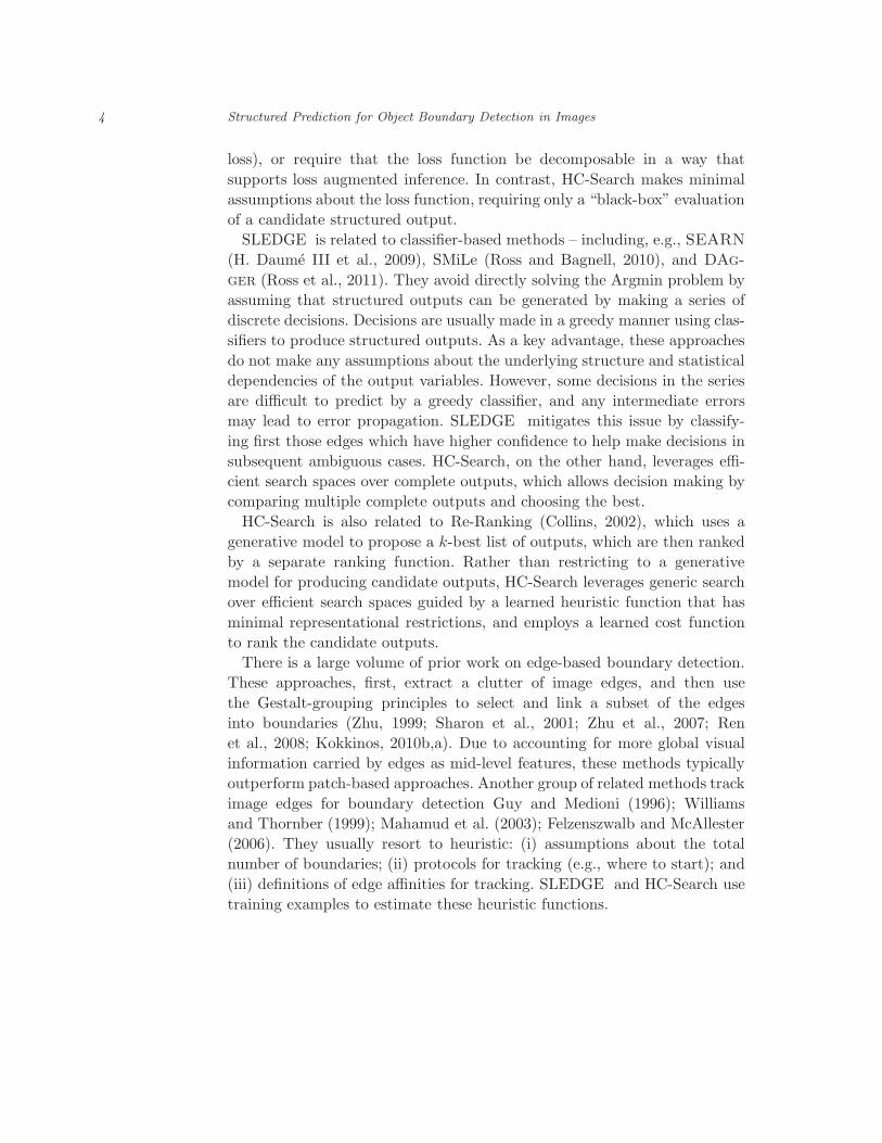
Figure 1.1: Overview: (a) The input image. (b) Edge detectors typically output aprobability edge map, which can be thresholded into a set of image edges. (c) Ourstructured prediction labels every edge as being on or off an object boundary. Thedarker the boundaries, the higher prediction confidence.

This problem can be cast within the structured prediction framework,

where image edges comprising the structured input are mapped to bound-

ary detections comprising the structured output. We use image edges as

features suitable for boundary detection. This is because boundaries typ-

ically coincide with a subset of edges, and edges provide rich information

about the spatial extent and layout of objects in the image. Thus, our struc-

tured prediction labels image edges as belonging to either a boundary or

background clutter, as illustrated in Figure 1.1.

In this paper, we consider two structured prediction algorithms aimed

at optimally combining intrinsic and layout properties of image edges for

boundary detection. First, SLEDGE is a policy iteration algorithm, pre-

sented in Payet and Todorovic (2013). It sequentially labels the edges, where

in each labeling step evidence about the Gestalt grouping of the edges is up-

dated based on previously detected boundaries. Training of SLEDGE is

iterative. In each iteration, SLEDGE labels a sequence of edges extracted

from each training image. This induces loss with respect to the ground truth.

The training sequences are then used as training examples for re-learning

SLEDGE in the next iteration, such that the total loss is minimized.

Second, Heuristic-Cost Search (HC-Search) is a structured prediction

algorithm based on search in the space of structured outputs (Doppa et al.,

2013, 2012). HC-Search uncovers high quality labelings of image edges (i.e.,

structured outputs), and represents them as nodes of a rooted tree. Links

in the tree correspond to moves from one candidate output to another. The

goal of HC-Search is to effectively search this tree in order to quickly find

an optimal output. To this end, we train a heuristic function to evaluate the

moves throughout the search tree, and a cost function to select an optimal

node in the tree among the candidates.

Both algorithms prove robust and effective, and compare favorably with

the state-of-the-art structured prediction methods, in terms of recall and pre-

1.2 Related Work 3

cision, on the following benchmark datasets: Berkeley segmentation datasets

BSD300 and BSD500 (Martin et al., 2001; Arbelaez et al., 2010), Weizmann

Horses (Borenstein and Ullman, 2002), and LabelMe (B.Russell et al., 2008).

HC-Search gives higher recall and precision, but at the cost of higher com-

plexity than SLEDGE.

In the following, Section 1.2 reviews prior work; Section 1.3 describes the

edge detector and edge properties used in this paper; Section 1.4 specifies

SLEDGE; Section 1.5 presents HC-Search; and Section 1.6 presents our

experimental evaluation.

1.2 Related Work

This section focuses on reviewing prior work on structured prediction, and

closely related work on edge-based boundary detection in images.

A standard approach to structured prediction is to learn a cost function

C(x,y) for scoring a structured output, y, given a structured input, x.

Computing C(x,y) involves solving the “Argmin” problem, which is to find

the minimum cost output for a given input:

Argmin: y = arg miny

C(x,y). (1.1)

Prior work has demonstrated that log-distributions of graphical models –

namely, Markov Random Fields (MRF) (Zhu, 1999) or Conditional Random

Fields (CRF) (Ren et al., 2008; Maire et al., 2008) – can be used to suitably

define C(x,y) in Eq. (1.1) for boundary detection. In general, exactly solving

the Argmin problem of Eq. (1.1) is intractable, including the cases when

C(x,y) is defined using MRFs or CRFs. This has been addressed using

heuristic optimization methods, such as, e.g., loopy belief propagation or

variational inference. While such methods have shown some success in

practice, the effect of their approximation on learning parameters of the

original models of C(x,y) – i.e., MRFs or CRFs – is poorly understood.

This is because learning of C(x,y) on training examples typically involves

inference as one of the necessary steps.

Another group of methods consider solving the Argmin problem via

cascading (Felzenszwalb and McAllester, 2007; Weiss and Taskar, 2010;

Munoz et al., 2010), where inference is run in stages from a coarse to fine

level of abstraction. These methods, however, have a number of limitations.

They place restrictions on the form of C(x,y) to facilitate cascading, which

may not be suitable for boundary detection. In particular, they typically

ignore the loss function of a problem (e.g., by assuming the Hamming


loss), or require that the loss function be decomposable in a way that

supports loss augmented inference. In contrast, HC-Search makes minimal

assumptions about the loss function, requiring only a “black-box” evaluation

of a candidate structured output.

SLEDGE is related to classifier-based methods – including, e.g., SEARN

(H. Daume III et al., 2009), SMiLe (Ross and Bagnell, 2010), and DAg-

ger (Ross et al., 2011). They avoid directly solving the Argmin problem by

assuming that structured outputs can be generated by making a series of

discrete decisions. Decisions are usually made in a greedy manner using clas-

sifiers to produce structured outputs. As a key advantage, these approaches

do not make any assumptions about the underlying structure and statistical

dependencies of the output variables. However, some decisions in the series

are difficult to predict by a greedy classifier, and any intermediate errors

may lead to error propagation. SLEDGE mitigates this issue by classify-

ing first those edges which have higher confidence to help make decisions in

subsequent ambiguous cases. HC-Search, on the other hand, leverages effi-

cient search spaces over complete outputs, which allows decision making by

comparing multiple complete outputs and choosing the best.

HC-Search is also related to Re-Ranking (Collins, 2002), which uses a

generative model to propose a k-best list of outputs, which are then ranked

by a separate ranking function. Rather than restricting to a generative

model for producing candidate outputs, HC-Search leverages generic search

over efficient search spaces guided by a learned heuristic function that has

minimal representational restrictions, and employs a learned cost function

to rank the candidate outputs.

There is a large volume of prior work on edge-based boundary detection.

These approaches, first, extract a clutter of image edges, and then use

the Gestalt-grouping principles to select and link a subset of the edges

into boundaries (Zhu, 1999; Sharon et al., 2001; Zhu et al., 2007; Ren

et al., 2008; Kokkinos, 2010b,a). Due to accounting for more global visual

information carried by edges as mid-level features, these methods typically

outperform patch-based approaches. Another group of related methods track

image edges for boundary detection Guy and Medioni (1996); Williams

and Thornber (1999); Mahamud et al. (2003); Felzenszwalb and McAllester

(2006). They usually resort to heuristic: (i) assumptions about the total

number of boundaries; (ii) protocols for tracking (e.g., where to start); and

(iii) definitions of edge affinities for tracking. SLEDGE and HC-Search use

training examples to estimate these heuristic functions.

1.3 Edge Extraction and Properties 5

1.3 Edge Extraction and Properties

Any low-level edge detector can be used for feature extraction in our

approach. In our experiments, we use: (a) Canny edge detector (Canny,

1986), or (b) gPb detector (Maire et al., 2008). gPb produces a probability

map of edge saliences. This map is thresholded at all probability levels, and

edges extracted using the standard non-maximum suppression. Given a set

of image edges, we extract their intrinsic properties and evidence about their

Gestalt grouping. In this paper, we use the same edge properties as those

described in Payet and Todorovic (2013). Below, we give a brief overview of

these properties, for completeness.

1.3.1 Intrinsic Edge Properties

The intrinsic edge properties, ψi=[ψi1, ψi2], include: (a) saliency, ψi1, and

(b) repeatability, ψi2. Salient edges are likely to belong to boundaries, and

repeating edges are more likely to arise from clutter and texture than

boundaries.

ψi1 is computed as the mean Pb value along an edge, ψi1 = meani(Pb),

for the gPb detector, or the mean of magnitude of intensity gradient along

the edge, ψi1 = meani(gradient), for the Canny detector.

For computing ψi2, we match all pairs of edges in the image. We estimate

the dissimilarity of two edges, sij, as a difference between their Shape

Context descriptors (Belongie et al., 2002). After linking all pairs of edges

and computing their dissimilarities, Page Rank (Brin and Page, 1998; Kim

et al., 2008; Lee and Grauman, 2009) iteratively estimates the degree of

repetition of each edge as ψi2 = (1− ρ) + ρ∑

jψj2

P

jsik

, where ρ = 0.85 is the

residual probability, and j and k the indices of neighboring edges to edge i.

For estimating the neighbors, we construct the Delaunay Triangulation (DT)

of all endpoints of the edges. If a pair of endpoints is connected in the DT

and directly “visible” to each other without crossing any other edge, then

their edges are declared as neighbors. This allows us to estimate proximity

and good continuation between even fairly distant edges in the image.

1.3.2 Layout Edge Properties

Layout properties are defined between pairs of neighboring image edges,

φij = [φij1, . . . ,φij5], and include standard formulations of the Gestalt

principles of grouping (Lowe, 1985; Zhu, 1999; Ren et al., 2008). Let Qi

and Qj denote the 2D coordinates of the closest endpoints of edges i and j.

We estimate:


q1

q2

!n1

!n2

α1

α2

(a)

r

r

r

(b)

Figure 1.2: (a) The line between symmetric points q1 and q2 lying on two distinctedges subtends the same angle α1 = α2 with the respective edge normals ~n1 and ~n2.(b) Constant distance r between symmetric points of two distinct edges indicatesparallelism of the edges.

1. Proximity as φij1 = 2π‖Qi−Qj‖2

min(len(i),len(j))2 , where len(·) measures the length of

an edge.

2. Collinearity as φij2 = |dθ(Qi)dQi

−dθ(Qj)dQj

|. θ(Q) ∈ [0, 2π] measures the angle

between the x-axis and the tangent of the edge at endpoint Q, where the

tangent direction is oriented towards the curve.

3. Co-Circularity as φij3 = |d2θ(Qi)dQ2

i

−d2θ(Qj)dQ2

j

|.

4. Symmetry as φij5 = meanq∈i

∣∣∣d2r(q)dq2

∣∣∣. As illustrated in Figure 1.2(a), two

points q1 ∈ i and q2 ∈ j are symmetric iff angles α1 = α2, where α1 is

subtended by line (q1, q2) and normal to i, and α2 is subtended by line

(q1, q2) and normal to j.

5. Parallelism as φij4 = meanq∈i

∣∣∣dr(q)

dq

∣∣∣. As illustrated in Figure 1.2(b),

parallelism is estimated as the mean of distance variations r(q) between

points q along edge i and their symmetric points on edge j.

To find symmetric points on two edges, we consider all pairs of points (q1, q2),

where q1 belongs to edge 1, and q2 belongs to edge 2, and compute their

cost matrix as a function of α1 and α2. We then use the standard Dynamic

Time Warping to find the best symmetric points.

By definition, we set φij = 0 for all edge pairs (i, j) that are not neighbors.

1.3.3 Helmholtz Principle of Edge Grouping

The Helmholtz principle of grouping (Helmholtz, 1962) is also used as one

of the edge properties. It is formalized as the entropy of a layout of edges.

When this entropy is low, the edges are less likely to belong to background

clutter.

The layout of edges can be characterized using the Voronoi diagram, as

presented in Ahuja and Todorovic (2008). Given a set of edges, we first

1.4 Sequential Labeling of Edges 7

compute the Voronoi tessellation for all pixels along the edges. Then, for

each edge i, we find a union of the Voronoi polygons γq of the edge’s pixels

q, resulting in a generalized Voronoi cell, Ui = ∪q∈iγq. The Voronoi cell

of edge i defines the relative area of its influence in the image, denoted

as Pi = area(Ui)/area(image). For n edges, we define the entropy of their

layout, H, as

H = −∑n

i=1 Pi logPi. (1.2)

Note that Pi depends on the length of i, and its position and orientation

relative to the other edges in the image. Since background clutter consists

of edges of different sizes, which are placed in different orientations, and at

various distances from the other edges, H of the clutter is likely to take

larger values than H of object boundaries. From our experiments presented

in Payet and Todorovic (2013), H of boundary layouts are in general lower

than those of background clutter.

1.3.4 Edge Descriptors

Without losing generality, we assume that from every image we can extract

a set of n edges V = {i : i = 1, . . . , n}. In our experiments, we set n = 200.

With every edge i ∈ V , we associate the descriptor xi defined as

xi = [ψi, [φi1, . . . ,φij , . . . ],H] (1.3)

where j ∈ V \{i}. The edge descriptors are used in our structured prediction

for boundary detection, as explained in the next two sections.

1.4 Sequential Labeling of Edges

This section describes how to conduct boundary detection as a sequential

labeling of image edges.

Let x = (x1,x2, . . . ,xn) ∈ X denote a sequence of edge descriptors that

are sequentially labeled in n steps, and y = (y1, y2, . . . , yn) ∈ Y denote

their corresponding binary labels, Y ∈ {0, 1}n. SLEDGE sequentially uses

a ranking function to select an edge k to be labeled yk = f(xk), and then

updates the descriptors of unlabeled edges, xi, i = k + 1, . . . , n, since they

depend on the layout of previously detected boundaries.

SLEDGE uses iterative batch-learning for estimating the structured pre-

diction f : X → Y, as summarized in Algorithm 1.1. The structured predic-


tion f is defined as

f (τ+1) =

{

h(τ+1) , with probability β ∈ [0, 1],

f (τ) , with probability (1 − β).(1.4)

In every learning iteration τ , the result of classification y(τ) = f (τ)(x) is

compared with ground truth y. This induces loss l(y(τ),y), which is then

used to learn a new classifier h(τ+1), and update f (τ+1) as in Eq. (1.4) with

probability β ∈ (0, 1]. This definition of f (τ) amounts to a probabilistic

sampling of individual classifiers h(1), h(2), . . . , h(τ). The classifier sampling

is governed by the multinomial distribution. From Eq. (1.4), the probability

of selecting classifier h(τ) in iteration T is

α(τ)T = βτ (1 − β)T−τ , τ = 1, 2, . . . , T. (1.5)

After τ reaches the maximum allowed number of iterations, T , the out-

put of learning is the last policy f (T ) from which h(1) is eliminated, i.e.,

the output is {h(2), h(3), . . . , h(T )} and their associated sampling probabil-

ities {κα(2)T , κα

(3)T , . . . , κα

(T )T }. The constant κ re-scales the α’s, such that

∑Tτ=2 κα

(τ)T = 1.

In the following, we specify two loss functions that can be used for learning

SLEDGE.

1.4.1 Two Loss Functions of SLEDGE

SLEDGE learns a labeling policy, f , that minimizes the expected loss over

all loss-sequences of sequential edge labeling in all training images. In this

section, we define two alternative loss functions.

First, we use the standard Hamming loss that counts the total number of

differences between predicted and ground-truth labels, y = (y1, . . . , yn) and

y = (y1, . . . , yn), as

LH(y,y) =

n∑

i=1

1 [yi 6= yi] , (1.6)

where 1 is the indicator function.

Since an error made at any edge carries the same relative weight, the

Hamming loss may guide SLEDGE to try to correctly label all small, non-

salient edges. To address this problem, we specify another loss function, LF ,

that uses the F -measure of recall and precision associated with a specific

edge. F -measure is one of the most common performance measures for

boundary detection (Martin et al., 2004). It is defined as the harmonic mean

of recall and precision of all image pixels that are detected as lying along

1.4 Sequential Labeling of Edges 9

Algorithm 1.1 Iterative Batch-Learning of SLEDGE

1: Input:2: The set of edges Vt of training images t = 1, 2, ...

3: Ground-truth labels of edges yt ∈ Y

4: Loss-sensitive classifier h, and initial h(1)

5: Loss function l

6: Interpolation constant β = 0.17: Maximum number of learning iterations T

8: Output:9: Learned policy f (T )

10:

11: f (1) = h(1)

12: for all training images t do

13: for all edges i ∈ Vt do

14: Compute x(1)t,i using intrinsic edge properties

15: Set layout edge properties in x(1)t,i to 0

16: end for

17: end for

18: for τ = 1 . . . T do

19: for all training images t do

20: for unlabeled edges in Vt do

21: Select unlabeled edge k ∈ Vt such that k = argmaxi∈Vtf (τ)(x

(τ)t,i )

22: Compute prediction y(τ)t,k = f (τ)(xt,k)

23: Update layout properties of unlabeled edges x(τ)t,i

24: end for

25: end for

26: Estimate loss over all training images l(y(τ)t ,yt)

27: Learn a new classifier h(τ+1)← h(X; l)

28: Compute f (τ+1) as in Eq. (1.4).29: end for

30: Return f (T ) without h(1).

an object boundary. A large value of F (y,y) indicates good precision and

recall, and corresponds to a low loss. Thus, we specify

LF (y,y) = 1 − F (y,y). (1.7)

Note that LH coarsely counts errors at the edge level, while LF is estimated

finely at the pixel level.

1.4.2 Majority Voting of SLEDGE

SLEDGE iteratively learns an optimal policy f , given by Eq. (1.4), which

represents a probabilistic mixture of classifiers {h(τ) : τ = 2, 3, . . . , T}.

Edges of a new image are sequentially labeled by weighted majority voting

of {h(τ)}, as described below. Voting decisions of several classifiers has been

shown to improve performance and reduces overfitting of each individual


classifier (Kittler et al., 1998; Dietterich, 2000; Freund et al., 2001).

For a given edge descriptor xi, we first run all classifiers {h(τ)(xi)}, and

then estimate the confidence of edge labeling yi ∈ {0, 1} as

P (f(xi) = yi) =T∑

τ=2

κα(τ)T P (h(τ)(xi) = yi), (1.8)

where the constant κ and α’s are given by Eq. (1.5), and P (h(τ)(xi)=y′) is

the confidence of classifier h(τ) when predicting the label of edge i. Finally,

SLEDGE classifies the edge as

yi = argmaxy′∈{0,1}

P (f(xi)=y′). (1.9)

1.5 HC-Search

Heuristic-Cost-Search (HC-Search) (Doppa et al., 2012, 2013) performs a

search-based structured prediction for a given structured input. Given a set

of edges and their descriptors x = {xi : i = 1, . . . , n}, HC-Search generates

a number of candidate outputs y, where input/output pairs s = (x, y)

represent states of a search space, s ∈ S, and then selects an optimal

state s = (x, y) as the solution. For exploring the search space, HC-Search

conducts a search procedure, π, guided by a heuristic function H, whereby

new states are generated based on the best previously visited state selected

by H. The generation of new states is specified by a generation function,

s′ = G(s), which is designed to flip low-confidence labels of edges in s,

and thus generate the new states s′. Finally, HC-Search uses a cost function

C(x,y) to return the least cost output y that is uncovered during the search.

The key elements of HC-Search include:

Search space over input/output pairs (x, y) ∈ S;

Search strategy π;

Heuristic function, H : X × Y 7→ R, for guiding the search toward high-

quality outputs;

Cost function, C : X×Y 7→ R, for scoring the candidate outputs generated

by the search.

Advantages of HC-Search relative to other structured prediction ap-

proaches, including CRFs, are as follows. First, it scales gracefully with the

complexity of the dependency structure of features. In particular, we are

free to increase the complexity of H and C (e.g., by including higher-order

1.5 HC-Search 11

features) without considering its impact on the inference complexity. The

work of Doppa et al. (2012, 2013) shows that the use of higher-order features

results in significant improvements. Second, the terms of the error decom-

position in Eq. (1.16) can be easily measured for a learned (H,C) pair,

which allows for an assessment of which function is more responsible for the

overall error. Third, HC-Search makes minimal assumptions about the loss

function, requiring only that we have a “black-box” evaluation of any can-

didate output. HC-Search can work with non-decomposable loss functions,

such as, e.g., F1 loss mentioned in Section 1.4.1.

In the following, we explain all these elements, and then describe how to

learn the heuristic and cost functions.

1.5.1 Key Elements of HC-Search

Search Space. A search space S is defined in terms of two functions: 1)

Initial state function, I(x), returns an initial state in S for input x; and

2) Generator function, G(s), returns for any state s a set of new states

{(x, y1), . . . , (x, yk)} that share the same input x.

The specific search space that we investigate leverages boundary predic-

tions made independently for every image edge by the logistic regression

classifier. Specifically, our I(x) corresponds to the logistic-regression predic-

tions of edge labels. G generates a set of next states in two steps. First, it

identifies a subset of image edges where the classifier has confidence lower

than a threshold. When gPb edges are used as input, the threshold is set to

0.5. Second, it generates one successor state for each low-confidence edge i

with the corresponding yi value flipped. We use the conditional probability

of the logistic regression as the confidence measure:

P (yi = 1|xi;wLR) = 1/(1 + exp(−w⊤LRxi)), (1.10)

where wLR are parameters of the logistic regression. Note that a particular

state may have a large number of successors, depending on P (yi = 1|xi;wLR)

values, whereas some other states may have only a few successors.

Search Strategy. The role of the search procedure π is to uncover high-

quality outputs, guided by the heuristic function H. Prior work of Doppa

et al. (2012, 2013) has shown that greedy search works quite well when used

with an effective search space. We investigate HC-Search with greedy search.

Given an input x, greedy search traverses a path of length τ through the

search space, selecting as the next state, the best successor of the current

state according to H. Specifically, if s(τ) is the state at search step τ , π selects

s(τ+1) = arg mins∈G(s(τ) H(s), where s(0) = I(x). We define the maximum

allowed number of search steps from one state to another as time bound τmax.


Note that τmax is equal to the number of good candidate states, selected by

H as parents for generating a number of successor states. Thus, the total

number of generated states during the search can be much larger than τ .

In this work, we define H following the standard formulation of CRF in

terms of unary and pairwise potential functions, Φ1 and Φ2, as

H(x,y)=∑

i∈V

w⊤H,1Φ1(xi, yi)+

∑

i,j∈V

w⊤H,2Φ2(xi,xj, yi, yj), (1.11)

where V is the set of input image edges, and w⊤H

= [w⊤H,1,w

⊤H,2] are

parameters of H. As standard, Φun(xi, yi) has non-zero elements in the

segment that corresponds to label yi, i.e., Φun(xi, 0) = [xi,0] or Φun(xi, 1) =

[0,xi]. The pairwise potential function is defined as

Φ2(xi,xj , yi, yj) =

{

0 , if yi = yj,

exp(−λ|xi − xj|2) , if yi 6= yj,

(1.12)

where λ is a parameter, set to λ = 1 in our experiments. Φ2 encourages

neighboring edges to take the same label. A similar formulation of the CRF

model for boundary detection is specified in Ren et al. (2008); Maire et al.

(2008).

Making Predictions. Given x, and a prediction time bound τ , HC-

Search traverses the search space starting at I(x), using the search procedure

π, guided by the heuristic function H, until the time bound is exceeded. It

then scores each visited state s according to C(s) and returns the y of the

lowest-cost state as the predicted output.

In this work, we define C to take the same form as H. In particular, we

specify

C(x,y)=∑

i∈V

w⊤C,1Φ1(xi, yi)+

∑

i,j∈V

w⊤C,2Φ2(xi,xj , yi, yj), (1.13)

where w⊤C

= [w⊤C,1,w

⊤C,2] are parameters of C.

1.5.2 Learning Heuristic and Cost Functions

Learning is aimed at training H and C such that the error of HC-Search,

ǫHC, is minimized over training data. ǫHC can be decomposed into two parts:

1) Generation error, ǫH, due to H not generating high-quality outputs; and

2) Selection error, ǫC|H, conditional on H, due to C not selecting the best

loss output generated by H. Our learning seeks to minimize ǫHC on training

data in a greedy stage-wise manner by first training H to minimize ǫH, and

then, training C to minimize ǫC|H conditioned on H. Below, we specify the

1.6 Results 13

error functions minimized in learning.

Let y∗H

denote the best output that HC-Search could possibly return when

using H, and y denote the output that it actually returns, and y denote

candidate outputs, and y denote the ground-truth output. Also, let YH(x)

be the set of candidate outputs generated using H for a given input x. Then,

we define

y∗H = arg miny∈YH(x)

L(x, y,y), (1.14)

y = arg miny∈YH(x)

C(x, y), (1.15)

where L(·) is a loss function. For HC-Search, we use only the Hamming loss,

specified in Eq. (1.6).

We decompose the error of HC-Search as

ǫHC = L (x,y∗H,y)︸︷︷︸

ǫH

+L (x, y,y) − L (x,y∗H,y)︸︷︷︸

ǫC|H

. (1.16)

H is trained by imitating search decisions made by the true loss available

for training data. We run the search procedure π for a time bound of τ for

input x using a heuristic equal to the true loss function, i.e. H(x, y) =

L(x, y,y). In addition, we record a set of ranking constraints that are

sufficient to reproduce the search behavior. For greedy search, at every

search step τ , we include one ranking constraint for every state (x, y) ∈

C(τ) \ (x, ybest), such that H(x, ybest) < H(x, y), where (x, ybest) is the best

state in the candidate set C(τ) (ties are broken by a random tie breaker).

The aggregate set of ranking examples is given to a rank learner – namely,

SVM-Rank (Joachims, 2006) – to learn H.

C is trained to score the outputs YH(x) generated by H according to their

true losses. Specifically, this training is formulated as a bi-partite ranking

problem to rank all the best loss outputs Ybest higher than all the non-best

loss outputs YH(x) \Ybest. For more details, the reader is referred to Doppa

et al. (2013).

1.6 Results

This section presents qualitative and quantitative evaluation of SLEDGE and

HC-Search on images from the BSD (Martin et al., 2001; Arbelaez et al.,

2010), Weizmann Horses (Borenstein and Ullman, 2002), and LabelMe

(B.Russell et al., 2008) datasets. BSD300 and BSD500 consist of 300 and

500 natural-scene images, respectively. They are manually segmented by a


number of different human annotators. The Weizmann Horses dataset con-

sists of 328 side-view images of horses that are also manually segmented.

For the LabelMe dataset, we select the 218 annotated images of the Boston

houses 2005 subset. The challenges of these datasets have been extensively

discussed in the past, and include, but are not limited to, clutter, illumina-

tion variations, occlusion. Below, we present our default training and testing

setups.

Training. We train SLEDGE and HC-Search on the 200 training images of

BSD300. For each image, we compute the edge probability map gPb (Maire

et al., 2008), and threshold the map so as to extract top 200 edges. We

compute edge intrinsic and layout properties as described in Section 1.3.

For training, we convert the manually annotated boundaries to ground-

truth labels for all edges in the training images: if more than 50% of an

edge length overlaps with a boundary then the ground-truth label of that

edge is 1; otherwise, the label is 0.

For SLEDGE, the initial classifier h(1) is a fully grown C4.5 decision

tree, that chooses the split attribute based on the normalized information

gain. The attributes considered for h(1) are only the intrinsic parameters ψi,

specified in Section 1.3.1. In further iterations of SLEDGE, the classifiers

h(τ) are pruned C4.5 decision trees, which are learned on all edge properties.

C4.5 pruning uses the standard confidence factor of 0.25. The interpolation

constant β, defined in Section 1.4, is set to β = 0.1. We use F1 loss function,

and voting to combine the output of the decision tree classifiers, as described

in Section 1.4.2.

For HC-Search, we use SVM-Rank (Joachims, 2006) to learn H and C

functions. The HC-Search results are obtained for the number of search

steps (i.e., time bound) τ = 100.

Testing and Comparison. Performance is measured as the average, pixel-

level precision and recall of the boundary map produced by SLEDGE or

HC-Search, as defined in Martin et al. (2004). We compare SLEDGE and

HC-Search with the latest work that uses standard structured-prediction

methods for boundary detection. Namely, for comparison, we use the CRF-

based method presented in Maire et al. (2008), and the F 3 boosting method

presented in Kokkinos (2010a). For fair comparison, we use the same set of

input image edges extracted using the Berkeley segmentation algorithm, as

described in Maire et al. (2008).

In the following, we first illustrate a few sample qualitative results of

boundary detection by SLEDGE and HC-Search on the BSD dataset. Then,

we evaluate SLEDGE and HC-Search using different: initial conditions, edge

1.6 Results 15

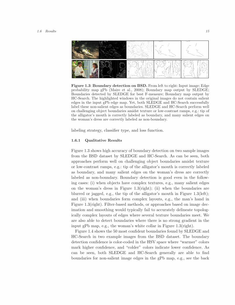
Figure 1.3: Boundary detection on BSD. From left to right: Input image; Edgeprobability map gPb (Maire et al., 2008); Boundary map output by SLEDGE;Boundaries detected by SLEDGE for best F-measure; Boundary map output byHC-Search. The highlighted windows in the original images do not contain salientedges in the input gPb edge map. Yet, both SLEDGE and HC-Search successfullylabel these non-salient edges as boundaries. SLEDGE and HC-Search perform wellon challenging object boundaries amidst texture or low-contrast ramps, e.g.: tip ofthe alligator’s mouth is correctly labeled as boundary, and many salient edges onthe woman’s dress are correctly labeled as non-boundary.

labeling strategy, classifier type, and loss function.

1.6.1 Qualitative Results

Figure 1.3 shows high accuracy of boundary detection on two sample images

from the BSD dataset by SLEDGE and HC-Search. As can be seen, both

approaches perform well on challenging object boundaries amidst texture

or low-contrast ramps, e.g.: tip of the alligator’s mouth is correctly labeled

as boundary, and many salient edges on the woman’s dress are correctly

labeled as non-boundary. Boundary detection is good even in the follow-

ing cases: (i) when objects have complex textures, e.g., many salient edges

on the woman’s dress in Figure 1.3(right); (ii) when the boundaries are

blurred or jagged, e.g., the tip of the alligator’s mouth in Figure 1.3(left);

and (iii) when boundaries form complex layouts, e.g., the man’s hand in

Figure 1.3(right). Filter-based methods, or approaches based on image dec-

imation and smoothing would typically fail to accurately delineate topolog-

ically complex layouts of edges where several texture boundaries meet. We

are also able to detect boundaries where there is no strong gradient in the

input gPb map, e.g., the woman’s white collar in Figure 1.3(right).

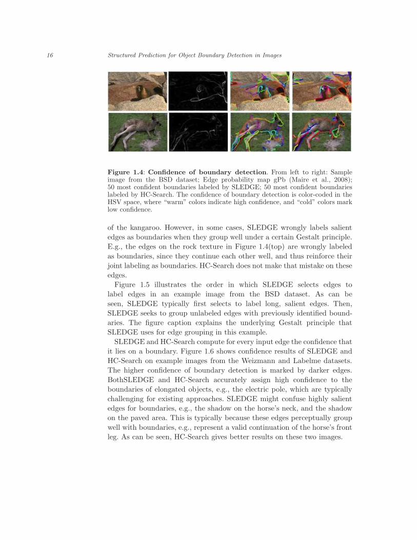
Figure 1.4 shows the 50 most confident boundaries found by SLEDGE and

HC-Search in two example images from the BSD dataset. The boundary

detection confidence is color-coded in the HSV space where “warmer” colors

mark higher confidence, and “colder” colors indicate lower confidence. As

can be seen, both SLEDGE and HC-Search generally are able to find

boundaries for non-salient image edges in the gPb map, e.g., see the back


Figure 1.4: Confidence of boundary detection. From left to right: Sampleimage from the BSD dataset; Edge probability map gPb (Maire et al., 2008);50 most confident boundaries labeled by SLEDGE; 50 most confident boundarieslabeled by HC-Search. The confidence of boundary detection is color-coded in theHSV space, where “warm” colors indicate high confidence, and “cold” colors marklow confidence.

of the kangaroo. However, in some cases, SLEDGE wrongly labels salient

edges as boundaries when they group well under a certain Gestalt principle.

E.g., the edges on the rock texture in Figure 1.4(top) are wrongly labeled

as boundaries, since they continue each other well, and thus reinforce their

joint labeling as boundaries. HC-Search does not make that mistake on these

edges.

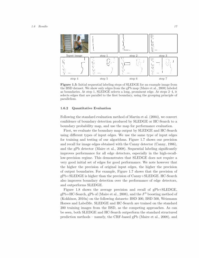
Figure 1.5 illustrates the order in which SLEDGE selects edges to

label edges in an example image from the BSD dataset. As can be

seen, SLEDGE typically first selects to label long, salient edges. Then,

SLEDGE seeks to group unlabeled edges with previously identified bound-

aries. The figure caption explains the underlying Gestalt principle that

SLEDGE uses for edge grouping in this example.

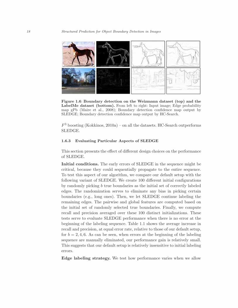
SLEDGE and HC-Search compute for every input edge the confidence that

it lies on a boundary. Figure 1.6 shows confidence results of SLEDGE and

HC-Search on example images from the Weizmann and Labelme datasets.

The higher confidence of boundary detection is marked by darker edges.

BothSLEDGE and HC-Search accurately assign high confidence to the

boundaries of elongated objects, e.g., the electric pole, which are typically

challenging for existing approaches. SLEDGE might confuse highly salient

edges for boundaries, e.g., the shadow on the horse’s neck, and the shadow

on the paved area. This is typically because these edges perceptually group

well with boundaries, e.g., represent a valid continuation of the horse’s front

leg. As can be seen, HC-Search gives better results on these two images.

1.6 Results 17

Input image step 1 step 2 step 3

step 4 step 5 step 6 step 7

Figure 1.5: Initial sequential labeling steps of SLEDGE for an example image fromthe BSD dataset. We show only edges from the gPb map (Maire et al., 2008) labeledas boundaries. At step 1, SLEDGE selects a long, prominent edge. At steps 2–4, itselects edges that are parallel to the first boundary, using the grouping principle ofparallelism.

1.6.2 Quantitative Evaluation

Following the standard evaluation method of Martin et al. (2004), we convert

confidence of boundary detection produced by SLEDGE or HC-Search to a

boundary probability map, and use the map for performance evaluation.

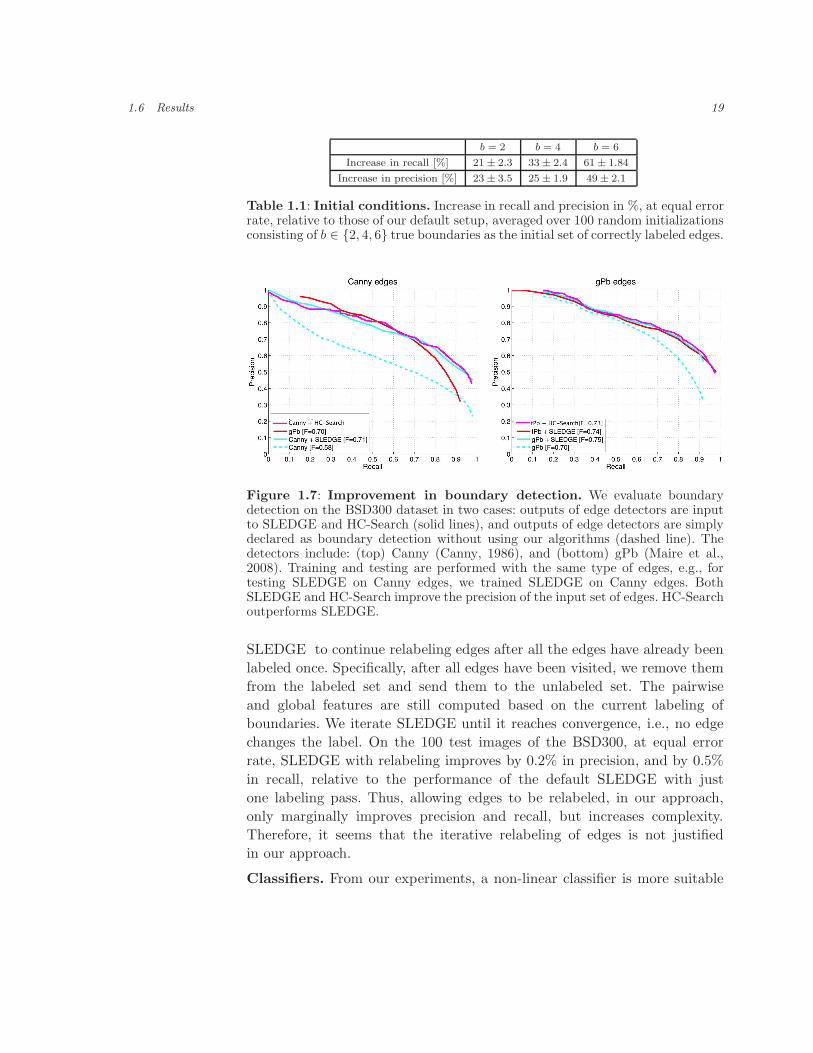
First, we evaluate the boundary map output by SLEDGE and HC-Search

using different types of input edges. We use the same type of input edges

for training and testing of our algorithms. Figure 1.7 shows our precision

and recall for image edges obtained with the Canny detector (Canny, 1986),

and the gPb detector (Maire et al., 2008). Sequential labeling significantly

improves performance for all edge detectors, especially in the high-recall-

low-precision regime. This demonstrates that SLEDGE does not require a

very good initial set of edges for good performance. We note however that

the higher the precision of original input edges, the higher the precision

of output boundaries. For example, Figure 1.7 shows that the precision of

gPb+SLEDGE is higher than the precision of Canny+SLEDGE. HC-Search

also improves boundary detection over the performance of edge detectors,

and outperforms SLEDGE.

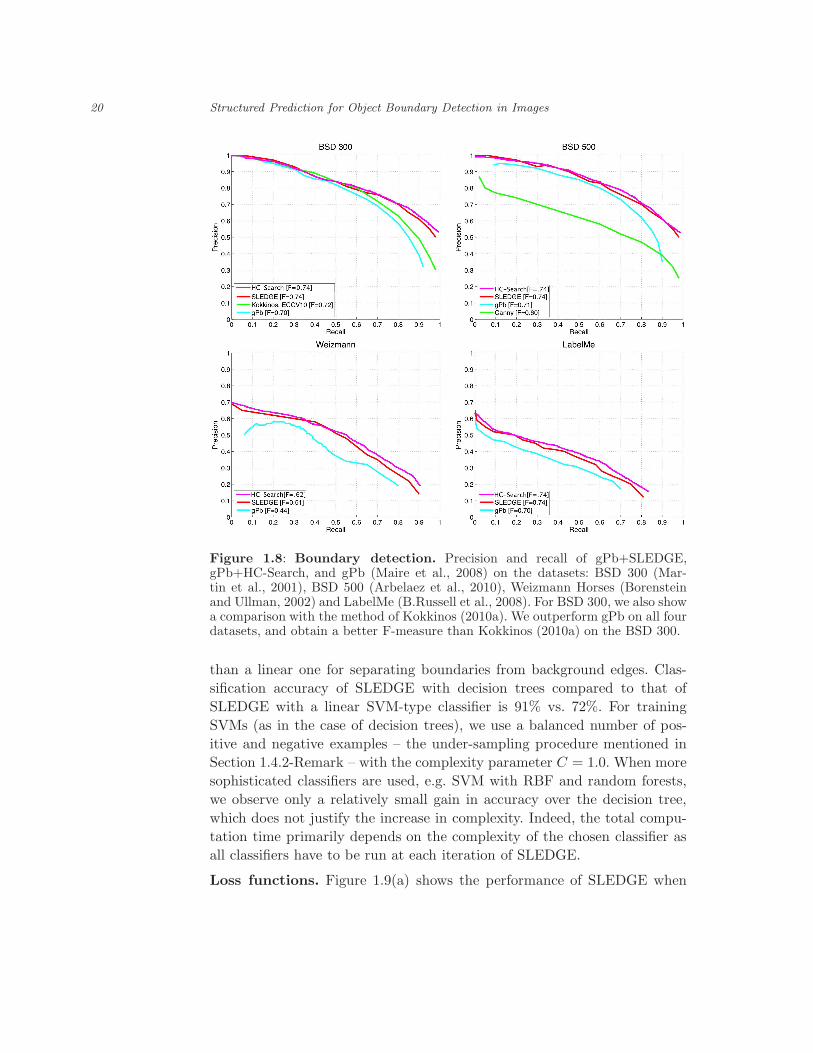
Figure 1.8 shows the average precision and recall of gPb+SLEDGE,

gPb+HC-Search, gPb of (Maire et al., 2008), and the F 3 boosting method of

(Kokkinos, 2010a) on the following datasets: BSD 300, BSD 500, Weizmann

Horses and LabelMe. SLEDGE and HC-Search are trained on the standard

200 training images from the BSD, as the competing approaches. As can

be seen, both SLEDGE and HC-Search outperform the standard structured

prediction methods – namely, the CRF-based gPb (Maire et al., 2008), and


Figure 1.6: Boundary detection on the Weizmann dataset (top) and theLabelMe dataset (bottom). From left to right: Input image; Edge probabilitymap gPb (Maire et al., 2008); Boundary detection confidence map output bySLEDGE; Boundary detection confidence map output by HC-Search.

F 3 boosting (Kokkinos, 2010a) – on all the datasets. HC-Search outperforms

SLEDGE.

1.6.3 Evaluating Particular Aspects of SLEDGE

This section presents the effect of different design choices on the performance

of SLEDGE.

Initial conditions. The early errors of SLEDGE in the sequence might be

critical, because they could sequentially propagate to the entire sequence.

To test this aspect of our algorithm, we compare our default setup with the

following variant of SLEDGE. We create 100 different initial configurations

by randomly picking b true boundaries as the initial set of correctly labeled

edges. The randomization serves to eliminate any bias in picking certain

boundaries (e.g., long ones). Then, we let SLEDGE continue labeling the

remaining edges. The pairwise and global features are computed based on

the initial set of randomly selected true boundaries. Finally, we compute

recall and precision averaged over these 100 distinct initializations. These

tests serve to evaluate SLEDGE performance when there is no error at the

beginning of the labeling sequence. Table 1.1 shows the average increase in

recall and precision, at equal error rate, relative to those of our default setup,

for b = 2, 4, 6. As can be seen, when errors at the beginning of the labeling

sequence are manually eliminated, our performance gain is relatively small.

This suggests that our default setup is relatively insensitive to initial labeling

errors.

Edge labeling strategy. We test how performance varies when we allow

1.6 Results 19

b = 2 b = 4 b = 6

Increase in recall [%] 21 ± 2.3 33 ± 2.4 61 ± 1.84

Increase in precision [%] 23 ± 3.5 25 ± 1.9 49 ± 2.1

Table 1.1: Initial conditions. Increase in recall and precision in %, at equal errorrate, relative to those of our default setup, averaged over 100 random initializationsconsisting of b ∈ {2, 4, 6} true boundaries as the initial set of correctly labeled edges.

Figure 1.7: Improvement in boundary detection. We evaluate boundarydetection on the BSD300 dataset in two cases: outputs of edge detectors are inputto SLEDGE and HC-Search (solid lines), and outputs of edge detectors are simplydeclared as boundary detection without using our algorithms (dashed line). Thedetectors include: (top) Canny (Canny, 1986), and (bottom) gPb (Maire et al.,2008). Training and testing are performed with the same type of edges, e.g., fortesting SLEDGE on Canny edges, we trained SLEDGE on Canny edges. BothSLEDGE and HC-Search improve the precision of the input set of edges. HC-Searchoutperforms SLEDGE.

SLEDGE to continue relabeling edges after all the edges have already been

labeled once. Specifically, after all edges have been visited, we remove them

from the labeled set and send them to the unlabeled set. The pairwise

and global features are still computed based on the current labeling of

boundaries. We iterate SLEDGE until it reaches convergence, i.e., no edge

changes the label. On the 100 test images of the BSD300, at equal error

rate, SLEDGE with relabeling improves by 0.2% in precision, and by 0.5%

in recall, relative to the performance of the default SLEDGE with just

one labeling pass. Thus, allowing edges to be relabeled, in our approach,

only marginally improves precision and recall, but increases complexity.

Therefore, it seems that the iterative relabeling of edges is not justified

in our approach.

Classifiers. From our experiments, a non-linear classifier is more suitable


Figure 1.8: Boundary detection. Precision and recall of gPb+SLEDGE,gPb+HC-Search, and gPb (Maire et al., 2008) on the datasets: BSD 300 (Mar-tin et al., 2001), BSD 500 (Arbelaez et al., 2010), Weizmann Horses (Borensteinand Ullman, 2002) and LabelMe (B.Russell et al., 2008). For BSD 300, we also showa comparison with the method of Kokkinos (2010a). We outperform gPb on all fourdatasets, and obtain a better F-measure than Kokkinos (2010a) on the BSD 300.

than a linear one for separating boundaries from background edges. Clas-

sification accuracy of SLEDGE with decision trees compared to that of

SLEDGE with a linear SVM-type classifier is 91% vs. 72%. For training

SVMs (as in the case of decision trees), we use a balanced number of pos-

itive and negative examples – the under-sampling procedure mentioned in

Section 1.4.2-Remark – with the complexity parameter C = 1.0. When more

sophisticated classifiers are used, e.g. SVM with RBF and random forests,

we observe only a relatively small gain in accuracy over the decision tree,

which does not justify the increase in complexity. Indeed, the total compu-

tation time primarily depends on the complexity of the chosen classifier as

all classifiers have to be run at each iteration of SLEDGE.

Loss functions. Figure 1.9(a) shows the performance of SLEDGE when

1.6 Results 21

0 0.1 0.2 0.3 0.4 0.5 0.6 0.7 0.8 0.9 10.5

0.6

0.7

0.8

0.9

1

Recall

Pre

cisi

on

LF [F=0.74]

LH

[F=0.72]

(a) Loss functions

0 0.1 0.2 0.3 0.4 0.5 0.6 0.7 0.8 0.9 10.4

0.5

0.6

0.7

0.8

0.9

1

Recall

Pre

cisi

on

Voting [F=0.74]Sampling [F=0.71]

(b) Interpolation schemes

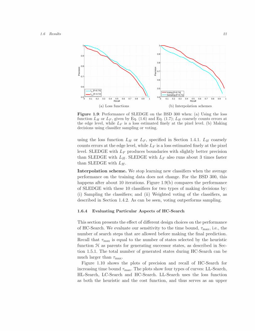
Figure 1.9: Performance of SLEDGE on the BSD 300 when: (a) Using the lossfunction LH or LF , given by Eq. (1.6) and Eq. (1.7); LH coarsely counts errors atthe edge level, while LF is a loss estimated finely at the pixel level. (b) Makingdecisions using classifier sampling or voting.

using the loss function LH or LF , specified in Section 1.4.1. LH coarsely

counts errors at the edge level, while LF is a loss estimated finely at the pixel

level. SLEDGE with LF produces boundaries with slightly better precision

than SLEDGE with LH . SLEDGE with LF also runs about 3 times faster

than SLEDGE with LH .

Interpolation scheme. We stop learning new classifiers when the average

performance on the training data does not change. For the BSD 300, this

happens after about 10 iterations. Figure 1.9(b) compares the performance

of SLEDGE with these 10 classifiers for two types of making decisions by:

(i) Sampling the classifiers; and (ii) Weighted voting of the classifiers, as

described in Section 1.4.2. As can be seen, voting outperforms sampling.

1.6.4 Evaluating Particular Aspects of HC-Search

This section presents the effect of different design choices on the performance

of HC-Search. We evaluate our sensitivity to the time bound, τmax, i.e., the

number of search steps that are allowed before making the final prediction.

Recall that τmax is equal to the number of states selected by the heuristic

function H as parents for generating successor states, as described in Sec-

tion 1.5.1. The total number of generated states during HC-Search can be

much larger than τmax.

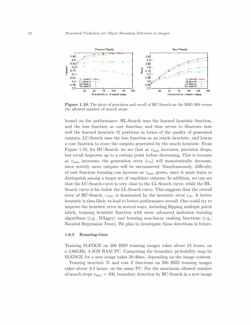
Figure 1.10 shows the plots of precision and recall of HC-Search for

increasing time bound τmax. The plots show four types of curves: LL-Search,

HL-Search, LC-Search and HC-Search. LL-Search uses the loss function

as both the heuristic and the cost function, and thus serves as an upper


Figure 1.10: The plots of precision and recall of HC-Search on the BSD 300 versusthe allowed number of search steps.

bound on the performance. HL-Search uses the learned heuristic function,

and the loss function as cost function, and thus serves to illustrate how

well the learned heuristic H performs in terms of the quality of generated

outputs. LC-Search uses the loss function as an oracle heuristic, and learns

a cost function to score the outputs generated by the oracle heuristic. From

Figure 1.10, for HC-Search, we see that as τmax increases, precision drops,

but recall improves up to a certain point before decreasing. This is because

as τmax increases, the generation error (ǫH) will monotonically decrease,

since strictly more outputs will be encountered. Simultaneously, difficulty

of cost function learning can increase as τmax grows, since it must learn to

distinguish among a larger set of candidate outputs. In addition, we can see

that the LC-Search curve is very close to the LL-Search curve, while the HL-

Search curve is far below the LL-Search curve. This suggests that the overall

error of HC-Search, ǫHC, is dominated by the heuristic error ǫH. A better

heuristic is thus likely to lead to better performance overall. One could try to

improve the heuristic error in several ways, including flipping multiple patch

labels, training heuristic function with more advanced imitation learning

algorithms (e.g., DAgger) and learning non-linear ranking functions (e.g.,

Boosted Regression Trees). We plan to investigate these directions in future.

1.6.5 Running-time

Training SLEDGE on 200 BSD training images takes about 24 hours, on

a 2.66GHz, 3.4GB RAM PC. Computing the boundary probability map by

SLEDGE for a new image takes 20-40sec, depending on the image content.

Training heuristic H and cost C functions on 200 BSD training images

takes about 3-4 hours, on the same PC. For the maximum allowed number

of search steps τmax = 100, boundary detection by HC-Search in a new image

1.7 Conclusion 23

takes about 2 minutes.

Our code is implemented in MATLAB, and is not fully optimized for

efficiency.

1.7 Conclusion

We have presented two structured prediction approaches to boundary detec-

tion in arbitrary images, called SLEDGE and HC-Search. Both approaches

take as input salient edges, and label these edges as belonging to a boundary.

SLEDGE is a sequential labeling algorithm, which learns how to optimally

combine Gestalt grouping cues and intrinsic edge properties for boundary

detection. HC-Search is a search based algorithm, which greedily explores

the space of candidate solutions guided by the heuristic function, and then

selects the minimum cost solution from all the candidates.

Our empirical evaluation demonstrates that both SLEDGE and HC-

Search outperform standard structured prediction approaches to boundary

detection on the benchmark datasets – specifically, the CRF-based method

gPb (Maire et al., 2008), and F 3 boosting (Kokkinos, 2010a). This is, in part,

because both SLEDGE and HC-Search avoid directly solving the Argmin

problem of structured prediction by generating structured outputs through:

(i) Making a series of discrete decisions in the case of SLEDGE; or (ii)

Searching the output space in the case of HC-Search. Both SLEDGE and

HC-Search employ training data to explicitly learn how to conduct inference

through making sequential decisions or searching the output space. This

learning for inference seems to improve upon common practice to use

heuristic approximations for solving the NP-hard Argmin problem. As a

key advantage over the other structured prediction methods, SLEDGE and

HC-Search do not make strong assumptions about the underlying structure

and statistical dependencies of the output variables.

We have observed that SLEDGE tends to favor good continuation of

strong edges, which works well in most cases, but fails when there is an

accidental alignment of object and background edges (e.g., shadows).

Our experimental results indicate that the overall error of the HC-Search

approach is dominated by the heuristic error. One could try to further

improve our current results with HC-Search by improving the heuristic

function. We are currently investigating this direction by employing more

effective search spaces, advanced imitation learning algorithms, and non-

linear representations (e.g., Boosted Regression Trees) for the heuristic and

cost functions. A better search space can be constructed by flipping the labels

of multiple edges rather than one at a time, thereby reducing the search


depth for imitation learning. In this paper, we have used exact imitation

to generate training examples for learning the heuristic function. Perhaps

using DAgger (Ross et al., 2011) would be a better method. Finally, we

have used SVM Rank to learn the heuristic and cost functions, but one could

try to use other rank learners such as boosting and trees.

Acknowledgements

This research has been sponsored in part by grant NSF IIS 1302700.

1.8 References

N. Ahuja and S. Todorovic. Connected segmentation tree – a joint representationof region layout and hierarchy. In Conf. Computer Vision Pattern Recognition,2008.

P. Arbelaez, M. Maire, C. Fowlkes, and J. Malik. Contour detection and hierarchicalimage segmentation. IEEE Trans. PAMI, 99(RapidPosts), 2010.

S. Belongie, J. Malik, and J. Puzicha. Shape matching and object recognition usingshape contexts. IEEE Trans. PAMI, 24(4):509–522, 2002.

E. Borenstein and S. Ullman. Class-specific, top-down segmentation. In EuropeanConf. Computer Vision, volume 2, pages 109–124, 2002.

S. Brin and L. Page. The anatomy of a large-scale hypertextual web search engine.In Seventh International World-Wide Web Conference (WWW 1998), 1998.

B.Russell, A. Torralba, K. Murphy, and W. Freeman. LabelMe: a database andweb-based tool for image annotation. Int. J. Computer Vision, 77(1-3):157–173,2008.

J. Canny. A computational approach to edge detection. IEEE Trans. PAMI, 8(6):679–698, 1986.

M. Collins. Ranking algorithms for named entity extraction: Boosting and thevoted perceptron. In Proceedings of Association for Computational Linguistics,2002.

T. Dietterich. Ensemble methods in machine learning. In Lecture Notes in ComputerScience, pages 1–15, 2000.

J. Doppa, A. Fern, and P. Tadepalli. Output space search for structured prediction.In Int. Conf. Machine Learning, 2012.

J. Doppa, A. Fern, and P. Tadepalli. HC-Search: Learning heuristics and cost func-tions for structured prediction. In AAAI Conference on Artificial Intelligence,2013.

P. Felzenszwalb and D. McAllester. A min-cover approach for finding salient curves.In Conf. Perceptual Organization Computer Vision, 2006.

P. Felzenszwalb and D. McAllester. The generalized A* architecture. Journal ofArtificial Intelligence Research, 29:153–190, 2007.

Y. Freund, Y. Mansour, and R. Schapire. Why averaging classifiers can protect

1.8 References 25

against overfitting. In Int. Workshop on Artificial Intelligence and Statistics,2001.

G. Guy and G. Medioni. Inferring global perceptual contours from local features.Int. J. Computer Vision, 20(1-2):113–133, 1996.

H. Daume III, J. Langford, and D. Marcu. Search-based structured prediction.Machine Learning Journal, 75(3):297–325, 2009.

H. Helmholtz. Treatise on physiological optics. New York: Dover; (first publishedin 1867), 1962.

T. Joachims. Training linear SVMs in linear time. In Int. Conf. KnowledgeDiscovery and Data Mining, pages 217–226, 2006.

G. Kim, C. Faloutsos, and M. Hebert. Unsupervised modeling of object categoriesusing link analysis techniques. In Conf. Computer Vision Pattern Recognition,June 2008.

J. Kittler, M. Hatef, R. Duin, and J. Matas. On combining classifiers. IEEE Trans.PAMI, 20:226–239, 1998.

I. Kokkinos. Boundary detection using F-measure-, Filter- and Feature- (F 3) boost.In European Conf. Computer Vision, 2010a.

I. Kokkinos. Highly accurate boundary detection and grouping. In Conf. ComputerVision Pattern Recognition, 2010b.

Y. Lee and K. Grauman. Shape discovery from unlabeled image collections. InConf. Computer Vision Pattern Recognition, 2009.

D. Lowe. Perceptual Organization and Visual Recognition. Kluwer AcademicPublishers, Norwell, MA, USA, 1985.

S. Mahamud, L. Williams, K. Thornber, and K. Xu. Segmentation of multiplesalient closed contours from real images. IEEE Trans. PAMI, 25(4):433–444,2003.

M. Maire, P. Arbelaez, C. Fowlkes, and J. Malik. Using contours to detectand localize junctions in natural images. In Conf. Computer Vision PatternRecognition, 2008.

D. Martin, C. Fowlkes, D. Tal, and J. Malik. A database of human segmentednatural images and its application to evaluating segmentation algorithms andmeasuring ecological statistics. In Int. Conf. Computer Vision, 2001.

D. Martin, C. Fowlkes, and J. Malik. Learning to detect natural image boundariesusing local brightness, color, and texture cues. IEEE Trans. PAMI, 26:530–549,2004.

D. Munoz, A. Bagnell, and M. Hebert. Stacked hierarchical labeling. In EuropeanConf. Computer Vision, 2010.

N. Payet and S. Todorovic. SLEDGE: Sequential labeling of image edges forboundary detection. Int. J. Computer Vision, 104(1):15–37, 2013.

X. Ren, C. Fowlkes, and J. Malik. Learning probabilistic models for contourcompletion in natural images. Int. J. Computer Vision, 77(1-3):47–63, 2008.

S. Ross and A. Bagnell. Efficient reductions for imitation learning. Journal ofMachine Learning Research - Proceedings Track, 9:661–668, 2010.

S. Ross, G. Gordon, and A. Bagnell. A reduction of imitation learning andstructured prediction to no-regret online learning. Journal of Machine LearningResearch - Proceedings Track, 15:627–635, 2011.


E. Sharon, A. Brandt, and R. Basri. Segmentation and boundary detectionusing multiscale intensity measurements. In Conf. Computer Vision PatternRecognition, pages 469–476, 2001.

D. Weiss and B. Taskar. Structured prediction cascades. Journal of MachineLearning Research - Proceedings Track, 9:916–923, 2010.

L. Williams and K. Thornber. A comparison of measures for detecting naturalshapes in cluttered backgrounds. Int. J. Computer Vision, 34(2-3):81–96, 1999.

Q. Zhu, G. Song, and J. Shi. Untangling cycles for contour grouping. In Int. Conf.Computer Vision, pages 1–8, 2007.

S.-C. Zhu. Embedding Gestalt laws in Markov random fields. IEEE Trans. PAMI,21(11):1170–1187, 1999.

advanced structured prediction - oregon state...

Documents