ADVANCED SUBSIDIARY GCE

MATHEMATICS (MEI) 4766Statistics 1

Candidates answer on the Answer Booklet

OCR Supplied Materials:

• 8 page Answer Booklet• Graph paper• MEI Examination Formulae and Tables (MF2)

Other Materials Required:None

Monday 25 January 2010

Morning

Duration: 1 hour 30 minutes

**

44

77

66

66

**

INSTRUCTIONS TO CANDIDATES

• Write your name clearly in capital letters, your Centre Number and Candidate Number in the spaces provided

on the Answer Booklet.• Use black ink. Pencil may be used for graphs and diagrams only.• Read each question carefully and make sure that you know what you have to do before starting your answer.• Answer all the questions.

• Do not write in the bar codes.• You are permitted to use a graphical calculator in this paper.• Final answers should be given to a degree of accuracy appropriate to the context.

INFORMATION FOR CANDIDATES

• The number of marks is given in brackets [ ] at the end of each question or part question.

• You are advised that an answer may receive no marks unless you show sufficient detail of the working toindicate that a correct method is being used.

• The total number of marks for this paper is 72.• This document consists of 8 pages. Any blank pages are indicated.

© OCR 2010 [H/102/2650] OCR is an exempt Charity

RP–9E16 Turn over

2

Section A (36 marks)

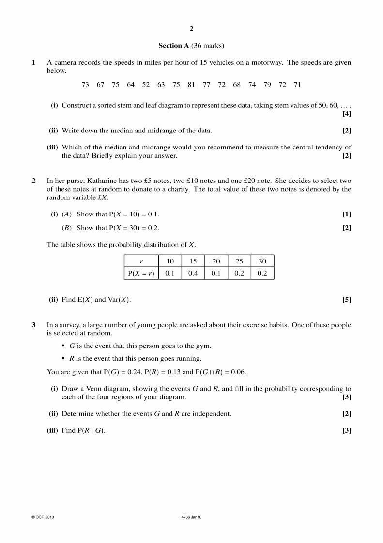
1 A camera records the speeds in miles per hour of 15 vehicles on a motorway. The speeds are given

below.

73 67 75 64 52 63 75 81 77 72 68 74 79 72 71

(i) Construct a sorted stem and leaf diagram to represent these data, taking stem values of 50, 60, … .

[4]

(ii) Write down the median and midrange of the data. [2]

(iii) Which of the median and midrange would you recommend to measure the central tendency of

the data? Briefly explain your answer. [2]

2 In her purse, Katharine has two £5 notes, two £10 notes and one £20 note. She decides to select two

of these notes at random to donate to a charity. The total value of these two notes is denoted by the

random variable £X.

(i) (A) Show that P(X = 10) = 0.1. [1]

(B) Show that P(X = 30) = 0.2. [2]

The table shows the probability distribution of X.

r 10 15 20 25 30

P(X = r) 0.1 0.4 0.1 0.2 0.2

(ii) Find E(X) and Var(X). [5]

3 In a survey, a large number of young people are asked about their exercise habits. One of these people

is selected at random.

• G is the event that this person goes to the gym.

• R is the event that this person goes running.

You are given that P(G) = 0.24, P(R) = 0.13 and P(G ∩ R) = 0.06.

(i) Draw a Venn diagram, showing the events G and R, and fill in the probability corresponding to

each of the four regions of your diagram. [3]

(ii) Determine whether the events G and R are independent. [2]

(iii) Find P(R | G). [3]

© OCR 2010 4766 Jan10

3

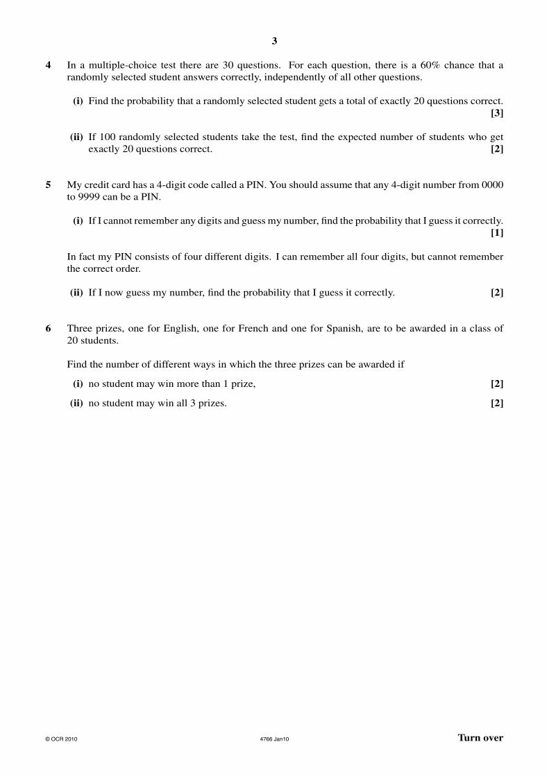
4 In a multiple-choice test there are 30 questions. For each question, there is a 60% chance that a

randomly selected student answers correctly, independently of all other questions.

(i) Find the probability that a randomly selected student gets a total of exactly 20 questions correct.

[3]

(ii) If 100 randomly selected students take the test, find the expected number of students who get

exactly 20 questions correct. [2]

5 My credit card has a 4-digit code called a PIN. You should assume that any 4-digit number from 0000

to 9999 can be a PIN.

(i) If I cannot remember any digits and guess my number, find the probability that I guess it correctly.

[1]

In fact my PIN consists of four different digits. I can remember all four digits, but cannot remember

the correct order.

(ii) If I now guess my number, find the probability that I guess it correctly. [2]

6 Three prizes, one for English, one for French and one for Spanish, are to be awarded in a class of

20 students.

Find the number of different ways in which the three prizes can be awarded if

(i) no student may win more than 1 prize, [2]

(ii) no student may win all 3 prizes. [2]

© OCR 2010 4766 Jan10 Turn over

4

Section B (36 marks)

7 A pear grower collects a random sample of 120 pears from his orchard. The histogram below shows

the lengths, in mm, of these pears.

0 60 70 80 90 1000

1

2

3

4

5

6

Length(mm)

Frequencydensity

(i) Calculate the number of pears which are between 90 and 100 mm long. [2]

(ii) Calculate an estimate of the mean length of the pears. Explain why your answer is only an

estimate. [4]

(iii) Calculate an estimate of the standard deviation. [3]

(iv) Use your answers to parts (ii) and (iii) to investigate whether there are any outliers. [4]

(v) Name the type of skewness of the distribution. [1]

(vi) Illustrate the data using a cumulative frequency diagram. [5]

© OCR 2010 4766 Jan10

5

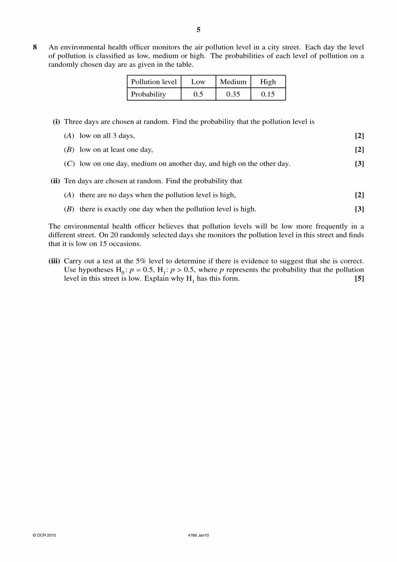
8 An environmental health officer monitors the air pollution level in a city street. Each day the level

of pollution is classified as low, medium or high. The probabilities of each level of pollution on a

randomly chosen day are as given in the table.

Pollution level Low Medium High

Probability 0.5 0.35 0.15

(i) Three days are chosen at random. Find the probability that the pollution level is

(A) low on all 3 days, [2]

(B) low on at least one day, [2]

(C) low on one day, medium on another day, and high on the other day. [3]

(ii) Ten days are chosen at random. Find the probability that

(A) there are no days when the pollution level is high, [2]

(B) there is exactly one day when the pollution level is high. [3]

The environmental health officer believes that pollution levels will be low more frequently in a

different street. On 20 randomly selected days she monitors the pollution level in this street and finds

that it is low on 15 occasions.

(iii) Carry out a test at the 5% level to determine if there is evidence to suggest that she is correct.

Use hypotheses H0: p = 0.5, H

1: p > 0.5, where p represents the probability that the pollution

level in this street is low. Explain why H1

has this form. [5]

© OCR 2010 4766 Jan10

6

BLANK PAGE

© OCR 2010 4766 Jan10

7

BLANK PAGE

© OCR 2010 4766 Jan10

8

Copyright Information

OCR is committed to seeking permission to reproduce all third-party content that it uses in its assessment materials. OCR has attempted to identify and contact all copyright holders

whose work is used in this paper. To avoid the issue of disclosure of answer-related information to candidates, all copyright acknowledgements are reproduced in the OCR Copyright

Acknowledgements Booklet. This is produced for each series of examinations, is given to all schools that receive assessment material and is freely available to download from our public

website (www.ocr.org.uk) after the live examination series.

If OCR has unwittingly failed to correctly acknowledge or clear any third-party content in this assessment material, OCR will be happy to correct its mistake at the earliest possible opportunity.

For queries or further information please contact the Copyright Team, First Floor, 9 Hills Road, Cambridge CB2 1GE.

OCR is part of the Cambridge Assessment Group; Cambridge Assessment is the brand name of University of Cambridge Local Examinations Syndicate (UCLES), which is itself a department

of the University of Cambridge.

© OCR 2010 4766 Jan10

4766 Mark Scheme January 2010

46

4766 Statistics 1

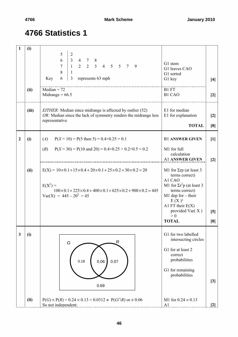
1 (i) 5 2 6 3 4 7 8 7 1 2 2 3 4 5 5 7 9 8 1 Key 6 3 represents 63 mph

G1 stem G1 leaves CAO G1 sorted G1 key [4]

(ii) Median = 72 Midrange = 66.5

B1 FT B1 CAO [2]

(iii)

EITHER: Median since midrange is affected by outlier (52) OR: Median since the lack of symmetry renders the midrange less representative

E1 for median E1 for explanation [2]

TOTAL [8]

2 (i) (A) P(X = 10) = P(5 then 5) = 0.4×0.25 = 0.1

(B) P(X = 30) = P(10 and 20) = 0.4×0.25 + 0.2×0.5 = 0.2

B1 ANSWER GIVEN M1 for full

calculation A1 ANSWER GIVEN

[1]

[2] (ii) E(X) = 10 0.1 15 0.4 20 0.1 25 0.2 30 0.2 20× + × + × + × + × =

E(X2) = 100 0.1 225 0.4 400 0.1 625 0.2 900 0.2 445× + × + × + × + × = Var(X) = 445 – 202 = 45

M1 for Σrp (at least 3 terms correct)

A1 CAO M1 for Σr2p (at least 3

terms correct) M1 dep for – their

E (X )² A1 FT their E(X)

provided Var( X ) > 0

[5]

TOTAL [8]

3 (i) G1 for two labelled

intersecting circles G1 for at least 2

correct probabilities

G1 for remaining

probabilities [3]

(ii) P(G) × P(R) = 0.24 × 0.13 = 0.0312 ≠ P(G∩R) or ≠ 0.06 So not independent.

M1 for 0.24 × 0.13 A1 [2]

0.18 0.06

0.69

G R

0.07

4766 Mark Scheme January 2010

47

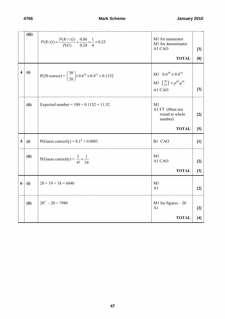
(iii)

( ) 0.06 1( | ) 0.25

( ) 0.24 4

P R GP R G

P G

∩= = = =

M1 for numerator M1 for denominator A1 CAO

[3]

TOTAL [8]

4 (i) P(20 correct) = 20 1030

0.6 0.4 0.115220

× × =

M1 0.620 × 0.410

M1 ( )3020 × p20 q10

A1 CAO

[3]

(ii) Expected number = 100 × 0.1152 = 11.52

M1 A1 FT (Must not

round to whole number)

[2]

TOTAL [5]

5 (i) P(Guess correctly) = 0.14 = 0.0001 B1 CAO [1]

(ii)

P(Guess correctly) = 1 1

4! 24=

M1 A1 CAO

[2]

TOTAL [3]

6 (i) 20 × 19 × 18 = 6840 M1

A1 [2]

(ii) 203 – 20 = 7980 M1 for figures – 20

A1 [2]

TOTAL [4]

4766 Mark Scheme January 2010

48

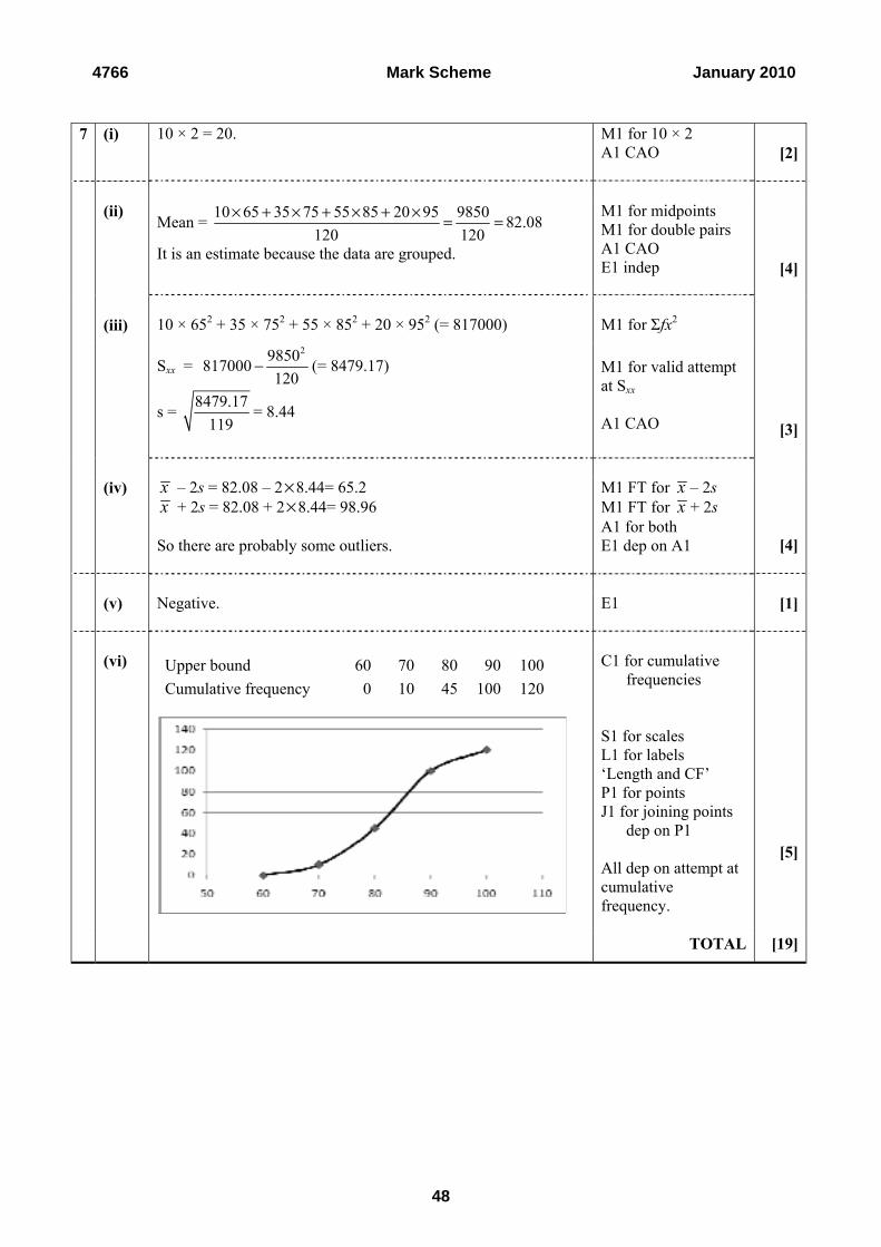
7 (i) 10 × 2 = 20. M1 for 10 × 2

A1 CAO [2]

(ii)

Mean = 10 65 35 75 55 85 20 95 9850

82.08120 120

× + × + × + × = =

It is an estimate because the data are grouped.

M1 for midpoints M1 for double pairs A1 CAO E1 indep

[4]

(iii)

10 × 652 + 35 × 752 + 55 × 852 + 20 × 952 (= 817000)

M1 for Σfx2

Sxx =

29850817000

120− (= 8479.17)

s = 8479.17

119= 8.44

M1 for valid attempt at Sxx A1 CAO [3]

(iv) x – 2s = 82.08 – 2×8.44= 65.2

x + 2s = 82.08 + 2×8.44= 98.96 So there are probably some outliers.

M1 FT for x – 2s M1 FT for x + 2s A1 for both E1 dep on A1

[4]

(v) Negative. E1

[1]

(vi) Upper bound 60 70 80 90 100

Cumulative frequency 0 10 45 100 120

C1 for cumulative frequencies

S1 for scales L1 for labels ‘Length and CF’ P1 for points J1 for joining points

dep on P1 All dep on attempt at cumulative frequency.

[5]

TOTAL [19]

4766 Mark Scheme January 2010

49

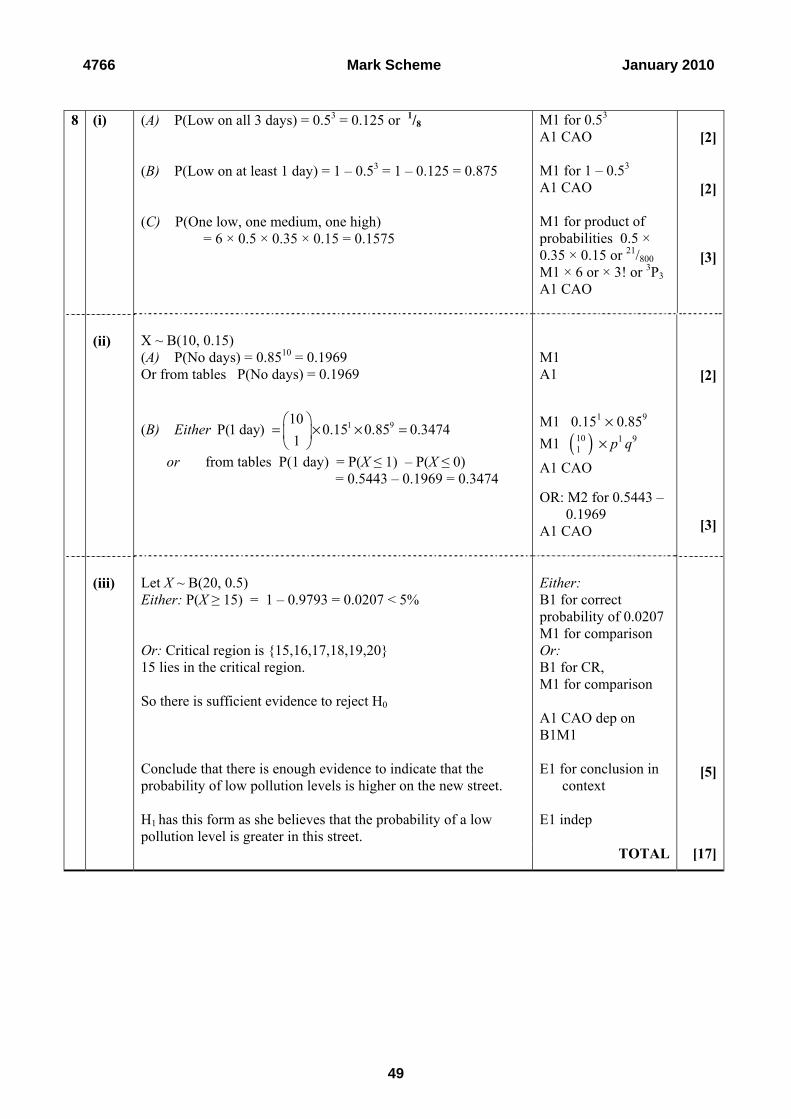
8 (i) (A) P(Low on all 3 days) = 0.53 = 0.125 or 1/8

(B) P(Low on at least 1 day) = 1 – 0.53 = 1 – 0.125 = 0.875 (C) P(One low, one medium, one high) = 6 × 0.5 × 0.35 × 0.15 = 0.1575

M1 for 0.53

A1 CAO M1 for 1 – 0.53 A1 CAO M1 for product of probabilities 0.5 × 0.35 × 0.15 or 21/800 M1 × 6 or × 3! or 3P3 A1 CAO

[2]

[2]

[3]

(ii)

X ~ B(10, 0.15) (A) P(No days) = 0.8510 = 0.1969 Or from tables P(No days) = 0.1969

(B) Either 1 910P(1 day) 0.15 0.85 0.3474

1

= × × =

or from tables P(1 day) = P(X ≤ 1) – P(X ≤ 0) = 0.5443 – 0.1969 = 0.3474

M1 A1

M1 0.151 × 0.859

M1 ( )101 × p1 q9

A1 CAO

OR: M2 for 0.5443 – 0.1969

A1 CAO

[2]

[3]

(iii) Let X ~ B(20, 0.5)

Either: P(X ≥ 15) = 1 – 0.9793 = 0.0207 < 5% Or: Critical region is {15,16,17,18,19,20} 15 lies in the critical region. So there is sufficient evidence to reject H0 Conclude that there is enough evidence to indicate that the probability of low pollution levels is higher on the new street. H1 has this form as she believes that the probability of a low pollution level is greater in this street.

Either: B1 for correct probability of 0.0207 M1 for comparison Or: B1 for CR, M1 for comparison A1 CAO dep on B1M1 E1 for conclusion in

context E1 indep

[5]

TOTAL [17]

Reports on the Units taken in January 2010

4766 Statistics 1 (G241 Z1)

General Comments The level of difficulty of the paper appeared to be entirely appropriate for the candidates with a good range of marks obtained. High-scoring candidates scored heavily on all questions with the exception of question 6; low-scoring candidates gained the majority of their marks from questions 1, 2 and 7. Very few candidates seemed totally unprepared. There seemed to be no trouble in completing the paper within the time allowed, and although the last parts of Q7 and Q8 were sometimes not completed this appeared to be due to a lack of knowledge rather than a lack of time. Most candidates supported their numerical answers with appropriate explanations and working although some rounding errors were noted, particularly in question 4. Arithmetic accuracy was generally good. Particularly amongst lower scoring candidates, there was evidence of the use of point probabilities in question 8. The Venn Diagram question was answered significantly better than in previous examinations with many candidates gaining full marks. Comments on Individual Questions 1 (i) There were many fully correct answers, but a significant number of candidates did

not include a key. Some used 50, 60, 70, 80 rather than 5, 6, 7, 8 for the stem, and others were not careful enough in aligning their leaves. Only a very small number of candidates did not know what a stem and leaf diagram was.

(ii) The median was almost always found correctly but many did not how to find the mid-

range, often giving (81-52)/2 = 14.5 as the answer. (iii) Most candidates identified the median as the preferred measure, often with a correct

explanation, but “middle of the data” was a common wrong answer. Those realising that outliers may be involved were more successful in explaining the reason for their choice than those using skewness. Some candidates thought that the mid-range was a measure of spread which did not help in their comparison.

2 (i) (A)(B) The response to this question was rather variable. Many stated that there are

5C2 = 10 combinations, then wrote 1/10 and 2/10 without explaining where the 1 and 2 came from, whereas others gave very clear explanations, which were often of the form 1/5 × ¼ × 2, 1/5 × ¼ × 4, 2/5 × ¼ × 2, etc. with no explanation of the 2 and 4 multipliers and benefit of doubt had to be given. Many others used a probability method, often giving creditable fractional/decimal multiplications to show the values necessary.

(ii) The vast majority of attempts at E(X) and Var(X) were correct. Only occasionally did

a candidate have no idea of how to go about this. There were also fewer instances of dividing by a spurious number or square rooting the answer than in the past.

32

Reports on the Units taken in January 2010

3 This question produced better answers overall than in previous series; with several candidates scoring full marks.

(i) This was very well answered although a fairly common error was to mark the regions

on the diagram with probabilities 0.24, 0.13 and 0.57 instead of 0.18, 0.07 and 0.69. Another error was to replace the 0.69 with 0.63.

(ii) The lack of independence of the two events was often correctly shown. Those

candidates with correct diagrams sometimes wrongly stated 0.18 × 0.07 ≠ 0.06. A small number confused independence with mutual exclusivity. Those who attempted to show that P(G|R) ≠ P(G|R') or similar often made mistakes finding the conditional probabilities.

(iii) The conditional probability was often found correctly, with or without correct

diagrams. However a considerable number of candidates tried to use the incorrect formula P(R|G) = P(R∩G) / P(R).

4 A large number of candidates scored full marks although a significant number of

candidates failed to realise that this was a binomial question.

(i) This was nearly always answered correctly. Omitting the 30C20 term was the only recurring mistake. A few very weak candidates just gave an answer of 0.620.

. (ii) The fact that the mean of a binomial distribution is np was well known. Rounding to a

whole number was common, usually 12, but sometimes 11. Some even stated "…because you can't have 0.52 of a student." Most did this after they had written a more accurate answer and did not lose marks. However in future series, rounding to the nearest whole number after getting a correct decimal answer may be penalised.

5 (i) Answers of 1/9999 and (1/9)4 were seen regularly as were attempts involving 1000C4

or 1000P4. Arithmetic errors such as 0.00001 or 1/1000 also occurred. (ii) Many correct answers were seen. However many candidates realised that 4! or 24

had some relevance but failed to produce the correct probability. These candidates often gave a final answer of 24 or alternatively divided 24 by 10000.

6 This proved beyond most candidates. Few scored full marks and a significant number

scored none. (i) 20C3 was a popular wrong answer; seen more often than the correct 20×19×18. (ii) Correct answers to this part were very rare, with a wide variety of wrong answers.

Amongst the more popular of these were 20 x 20 x 19 = 7600 and 6840 + 20 x 19 = 7220.

33

Reports on the Units taken in January 2010

7 (i) Very few wrong answers were seen. (ii) Most candidates used the correct frequencies and found the mean as 9850/120,

usually approximated to 82.08 or 82.1. However a significant number of attempts used frequencies of 1, 3.5, 5.5 and 2 (the frequency densities). Use of class boundaries or incorrect mid points was rare. Most candidates correctly stated that their answer was only an estimate because they were using the mid-points of the intervals.

(iii) The standard deviation was often found correctly although not always accurately due

to using 82.1 or just 82 for the mean. Only a few candidates divided by n rather than n – 1, so finding the RMSD rather than standard deviation. A number of candidates misinterpreted Σ fx2, and instead used one of Σx2, Σ(fx)2, Σ xf 2, (Σfx)2 or even Σf Σx2. Attempts at Σ(x - x )2f usually failed but some correct answers were achieved this way. As in part (ii) some candidates used frequency densities. The quickest way to find both mean and standard deviation was by use of calculator and a number of candidates used this method.

(iv) The formula for outliers of x ± 2s was well known and most candidates scored at

least the method marks by following through with their x and s, but there were some who insisted on using 1.5s. The conclusion as to whether there were outliers was often incorrect, many stating there were outliers rather than introducing the idea of doubt. Only a very few attempted to use quartiles and interquartile range to find outliers.

(v) Nearly all candidates stated that there was negative skewness, with only a few

suggesting it was positive or in some cases describing it as unimodal. (vi) Most candidates attempted a sensible cumulative frequency curve with the main and

surprisingly frequent error being plotting at the mid-points rather than the upper class boundary of the intervals. The other common error was the omission of the point (60,0) or replacing it with (0,0). Labelling was better than in the past, at least most wrote something on both axes. It would be helpful to see all candidates give the cumulative frequency values in a table before they drew the graph. Very few who drew graphs failed to realise the shape of graph required. Some centres appeared not to provide graph paper, whilst some candidates obviously preferred not to use it.

8 (i) (A) Almost all candidates answered this correctly.

(i) (B) Answers to this fell into two roughly equal groups; those who realised that

"medium or high" could be treated as one (i.e. "not low") and those who did not. The first group nearly always got the right answer. The second nearly always got the wrong answer. Attempts at exhaustive listings of LMH, LMM, MLH, MHL, …seldom included all 19 outcomes. The majority of correct answers were from candidates who simply calculated 1 – P(Low on no days).

(i) (C) Most candidates multiplied the three probabilities 0.5×0.35×0.15 but a lot left it at

that or multiplied by 3 or cubed it. Another not infrequent wrong answer involved (3C1 x 0.52 x 0.5) x (3C1 x 0.652 x 0.35) x (3C1 x 0.852 x 0.15) = 0.0541.

34

Reports on the Units taken in January 2010

35

plained.

(ii) Here most did recognise that "low or medium" could be grouped together as "not high" and used the binomial, B(10, 0.15).

(A) There were very many fully correct answers usually from binomial expressions, but also occasionally from tables.

(B) There was more use of tables here but still the majority of candidates calculated the answer. Some failed to remember to include the binomial coefficient 10C1.

(iii) The correct hypotheses and test value of 15 were given. Many candidates could not

correctly find P(X ≥ 15). P(X ≥ 15) = 1 – P(X ≤ 15) leading to 0.0059 was widespread; certainly more common than using the point probability, which was also often seen. Attempts at the critical region often showed similar problems with upper tail probabilities; many attempts resulting in {14,15,16,17,18,19,20}. Some candidates totally omitted a conclusion in context. The reason for H1 being p > 0.5 was generally well ex