advanced techniques for synthetic aperture radar
TRANSCRIPT

ADVANCED TECHNIQUES FOR SYNTHETIC APERTURE RADAR IMAGERECONSTRUCTION
By
DUC H. VU
A DISSERTATION PRESENTED TO THE GRADUATE SCHOOLOF THE UNIVERSITY OF FLORIDA IN PARTIAL FULFILLMENT
OF THE REQUIREMENTS FOR THE DEGREE OFDOCTOR OF PHILOSOPHY
UNIVERSITY OF FLORIDA
2012

c⃝ 2012 Duc H. Vu
2

To God and family
3

ACKNOWLEDGMENTS
This dissertation, and this academic journey would have not been possible without
the support of many people. I would like to take this space to thank first of all my
parents. Your guidance and infinite sacrifices enabled me to be at my full potential.
Without your love and support I would not be able to take on this journey. I would like
to thank my advisor, Jian Li, her patience and work ethics is inspiring. I will always be
grateful for all the discussions that we had; each one have made me a better researcher
and a better human being. I would like to thank my mentor, coworker and friend,
Oliver Allen. Your selflessness made possible this pursuit of knowledge and your
encouragement enabled an achievement that I never thought could be possible.
I would like to thank my friends and fellow lab mates of the Spectral Analysis
Laboratory: Hao, Jun, Bill, Xing, Zhaofu, Tarik, Ming, Lin, Enrique, Matteo, Xiang, Yubo,
Arsen, Erik, Yuanxiang, Kexin, Qilin, Xianqi, Bin, Luzhou, Ode, Will and Johan. For
the small span of time our life has overlapped, our time and friendship will never be
forgotten. Last but not least, I would like to thank my committee members: Dr. Henry
Zmuda, Dr. Jenshan Lin and Dr. Mingzhou Ding, for their time and guidance.
4

TABLE OF CONTENTS
page
ACKNOWLEDGMENTS . . . . . . . . . . . . . . . . . . . . . . . . . . . . . . . . . . 4
LIST OF TABLES . . . . . . . . . . . . . . . . . . . . . . . . . . . . . . . . . . . . . . 7
LIST OF FIGURES . . . . . . . . . . . . . . . . . . . . . . . . . . . . . . . . . . . . . 8
ABSTRACT . . . . . . . . . . . . . . . . . . . . . . . . . . . . . . . . . . . . . . . . . 10
CHAPTER
1 INTRODUCTION TO SYNTHETIC APERTURE RADAR . . . . . . . . . . . . . 13
1.1 The Signal Processing Aspect of SAR . . . . . . . . . . . . . . . . . . . . 151.2 Resolution in Range . . . . . . . . . . . . . . . . . . . . . . . . . . . . . . 15
1.2.1 Matched Filtering . . . . . . . . . . . . . . . . . . . . . . . . . . . . 171.2.2 Pulse Compression . . . . . . . . . . . . . . . . . . . . . . . . . . . 211.2.3 Linear Frequency Modulated Signal . . . . . . . . . . . . . . . . . 21
1.3 Resolution in Cross Range . . . . . . . . . . . . . . . . . . . . . . . . . . 251.3.1 Synthetic Aperture . . . . . . . . . . . . . . . . . . . . . . . . . . . 261.3.2 Processing of the Return Signals . . . . . . . . . . . . . . . . . . . 30
2 SAR RECONSTRUCTION USING A BAYESIAN APPROACH . . . . . . . . . . 33
2.1 Preliminaries and Data Model . . . . . . . . . . . . . . . . . . . . . . . . . 362.2 Data-Adaptive Algorithms . . . . . . . . . . . . . . . . . . . . . . . . . . . 40
2.2.1 Compressed Sampling Matching Pursuit (CoSaMP) . . . . . . . . 402.2.2 Iterative Adaptive Approach (IAA) . . . . . . . . . . . . . . . . . . . 412.2.3 Sparse Learning via Iterative Minimization (SLIM) . . . . . . . . . . 41
2.3 Numerical Examples . . . . . . . . . . . . . . . . . . . . . . . . . . . . . . 432.3.1 An Example of Ideal Point Scatterers . . . . . . . . . . . . . . . . . 442.3.2 Imaging of the Backhoe . . . . . . . . . . . . . . . . . . . . . . . . 452.3.3 3-D SAR Imaging . . . . . . . . . . . . . . . . . . . . . . . . . . . . 45
3 SAR RECONSTRUCTION OF INTERRUPTED DATA . . . . . . . . . . . . . . 50
3.1 Nonparametric Spectral Analysis . . . . . . . . . . . . . . . . . . . . . . . 533.1.1 Data Model . . . . . . . . . . . . . . . . . . . . . . . . . . . . . . . 533.1.2 Iterative Adaptive Approach (IAA) . . . . . . . . . . . . . . . . . . . 543.1.3 Sparse Learning via Iterative Minimization (SLIM) . . . . . . . . . . 553.1.4 Computational Complexities and Memory Requirements . . . . . . 57
3.2 Missing Data Spectral Analysis and Fast Implementations . . . . . . . . . 583.2.1 Data Model . . . . . . . . . . . . . . . . . . . . . . . . . . . . . . . 583.2.2 Fast Iterative Adaptive Approach (Fast-IAA) . . . . . . . . . . . . . 61
3.2.2.1 Efficient Computation of the IAA Covariance Matrix . . . 613.2.2.2 Efficient Computation of B . . . . . . . . . . . . . . . . . 62
5

3.2.3 Fast SLIM Using Conjugate Gradient (CG-SLIM) . . . . . . . . . . 643.2.4 Fast SLIM Using the Gohberg-Semencul-Type Formula (GS-SLIM) 67
3.3 Numerical Examples . . . . . . . . . . . . . . . . . . . . . . . . . . . . . . 723.3.1 1-D Spectral Estimation . . . . . . . . . . . . . . . . . . . . . . . . 723.3.2 2-D Interrupted SAR Imaging . . . . . . . . . . . . . . . . . . . . . 78
4 SAR GROUND MOVING TARGET INDICATION . . . . . . . . . . . . . . . . . 84
4.1 Geometry and Data Model . . . . . . . . . . . . . . . . . . . . . . . . . . 854.2 Array Calibration . . . . . . . . . . . . . . . . . . . . . . . . . . . . . . . . 88
4.2.1 Distances Among Antennas . . . . . . . . . . . . . . . . . . . . . . 894.2.2 Antenna Gains . . . . . . . . . . . . . . . . . . . . . . . . . . . . . 90
4.3 Ground Moving Target Indication (GMTI) . . . . . . . . . . . . . . . . . . . 914.3.1 Ground Clutter Cancelation Using RELAX . . . . . . . . . . . . . . 924.3.2 Moving Target Detection Using IAA . . . . . . . . . . . . . . . . . . 94
4.4 Analysis of the AFRL GOTCHA Data Set . . . . . . . . . . . . . . . . . . 964.4.1 Description of the AFRL Gotcha GMTI Data Set . . . . . . . . . . . 964.4.2 SAR Imaging . . . . . . . . . . . . . . . . . . . . . . . . . . . . . . 984.4.3 Array Calibration . . . . . . . . . . . . . . . . . . . . . . . . . . . . 984.4.4 Velocity Ambiguity Analysis . . . . . . . . . . . . . . . . . . . . . . 994.4.5 Adaptive GMTI . . . . . . . . . . . . . . . . . . . . . . . . . . . . . 101
5 MULTIPLE-INPUT MULTIPLE-OUTPUT SAR GMTI . . . . . . . . . . . . . . . 107
5.1 Existing GMTI Methods . . . . . . . . . . . . . . . . . . . . . . . . . . . . 1075.2 MIMO GMTI System Model . . . . . . . . . . . . . . . . . . . . . . . . . . 108
5.2.1 Scene of Interest . . . . . . . . . . . . . . . . . . . . . . . . . . . . 1095.2.2 Antenna Array and Transmission Waveforms . . . . . . . . . . . . 1095.2.3 Received Signal Model . . . . . . . . . . . . . . . . . . . . . . . . . 110
5.3 GMTI Algorithm . . . . . . . . . . . . . . . . . . . . . . . . . . . . . . . . . 1115.3.1 Range Compression . . . . . . . . . . . . . . . . . . . . . . . . . . 1115.3.2 Doppler Processing and Phase Compensation . . . . . . . . . . . 1125.3.3 Moving Target Detection in the Range-Doppler-Velocity Domain . . 113
5.4 Numerical Examples . . . . . . . . . . . . . . . . . . . . . . . . . . . . . . 1155.4.1 Single-Input and Multiple-Output (SIMO) System . . . . . . . . . . 1165.4.2 Multiple-Input and Multiple-Output (MIMO) System . . . . . . . . . 117
6 CONCLUDING REMARKS AND FUTURE WORKS . . . . . . . . . . . . . . . 121
REFERENCES . . . . . . . . . . . . . . . . . . . . . . . . . . . . . . . . . . . . . . . 123
BIOGRAPHICAL SKETCH . . . . . . . . . . . . . . . . . . . . . . . . . . . . . . . . 131
6

LIST OF TABLES
Table page
3-1 Computation times needed by IAA, SLIM and their fast implementations. . . . . 77
3-2 Computation times needed by IAA, SLIM and their fast implementations forinterrupted SAR imaging under various interruption conditions. . . . . . . . . . 79
4-1 Target velocity versus fv . . . . . . . . . . . . . . . . . . . . . . . . . . . . . . . . 100
7

LIST OF FIGURES
Figure page
1-1 Resolution of a pixel . . . . . . . . . . . . . . . . . . . . . . . . . . . . . . . . . 16
1-2 Scene with Impulse Targets . . . . . . . . . . . . . . . . . . . . . . . . . . . . . 16
1-3 Transmitted Signal . . . . . . . . . . . . . . . . . . . . . . . . . . . . . . . . . . 18
1-4 Returned Signal . . . . . . . . . . . . . . . . . . . . . . . . . . . . . . . . . . . 18
1-5 Matched Filter of Return Signals . . . . . . . . . . . . . . . . . . . . . . . . . . 19
1-6 Two Close Targets . . . . . . . . . . . . . . . . . . . . . . . . . . . . . . . . . . 20
1-7 Returned Signals of Two Close Targets . . . . . . . . . . . . . . . . . . . . . . 20
1-8 Matched Filter Return of Two Close Targets . . . . . . . . . . . . . . . . . . . . 20
1-9 Example of a Chirp Signal . . . . . . . . . . . . . . . . . . . . . . . . . . . . . . 22
1-10 Sinc Function . . . . . . . . . . . . . . . . . . . . . . . . . . . . . . . . . . . . . 24
1-11 Return From Scene Due to a Chirp . . . . . . . . . . . . . . . . . . . . . . . . . 24
1-12 Returns from Scene After Matched Filtering for a Chirp . . . . . . . . . . . . . 24
1-13 Cross Range Width of a Real Aperture Antenna . . . . . . . . . . . . . . . . . 25
1-14 Concept of Doppler . . . . . . . . . . . . . . . . . . . . . . . . . . . . . . . . . 26
1-15 Doppler Resolution . . . . . . . . . . . . . . . . . . . . . . . . . . . . . . . . . . 27
1-16 Cross Range Width of a Real Aperture Antenna . . . . . . . . . . . . . . . . . 29
2-1 SAR imaging schematics. . . . . . . . . . . . . . . . . . . . . . . . . . . . . . . 36
2-2 Imaging of Scatterers . . . . . . . . . . . . . . . . . . . . . . . . . . . . . . . . 46
2-3 Visualizing the Backhoe Dataset . . . . . . . . . . . . . . . . . . . . . . . . . . 47
2-4 Backhoe 3-D SAR Image Reconstruction . . . . . . . . . . . . . . . . . . . . . 48
2-5 Fused 3-D image using SLIM . . . . . . . . . . . . . . . . . . . . . . . . . . . . 48
3-1 Nonparametric spectral estimation without and with missing samples . . . . . . 74
3-2 Nonparametric spectral estimates for data sequences with missing samples . . 75
3-3 Missing samples estimation . . . . . . . . . . . . . . . . . . . . . . . . . . . . . 76
3-4 Nonparametric spectral estimates for data sequences with missing samplesusing SLIM-IAA . . . . . . . . . . . . . . . . . . . . . . . . . . . . . . . . . . . . 77
8

3-5 Slicy object and benchmark SAR image . . . . . . . . . . . . . . . . . . . . . . 78
3-6 Modulus of the SAR images of the Slicy object obtained from a 40×40 completedata matrix. . . . . . . . . . . . . . . . . . . . . . . . . . . . . . . . . . . . . . . 80
3-7 SAR images of the Slicy object under random 68% data loss. . . . . . . . . . . 81
3-8 SAR images of the Slicy object under random 30% data loss. . . . . . . . . . . 82
4-1 Geometry of an airbore multi-channel SAR system. . . . . . . . . . . . . . . . . 86
4-2 The flow chart of the entire processing chain for the proposed adaptive SARbased GMTI. . . . . . . . . . . . . . . . . . . . . . . . . . . . . . . . . . . . . . 96
4-3 AFRL Gotcha data scene setup . . . . . . . . . . . . . . . . . . . . . . . . . . . 97
4-4 SAR images of the 46th second . . . . . . . . . . . . . . . . . . . . . . . . . . 99
4-5 Estimated distance between Antennas. . . . . . . . . . . . . . . . . . . . . . . 100
4-6 Spectral windows for the array geometry of the AFRL Gotcha GMTI system. . . 101
4-7 GMTI results of DPCA at the 46th second. . . . . . . . . . . . . . . . . . . . . . 103
4-8 GMTI results of ATI at the 46th second. . . . . . . . . . . . . . . . . . . . . . . 103
4-9 GMTI results of IAA at the 46th second. . . . . . . . . . . . . . . . . . . . . . . 104
4-10 GMTI results using IAA with all three antennas at the 46th second . . . . . . . 105
4-11 GMTI results using IAA with all three antennas at the 51st and the 68th second. 105
5-1 Illustration of ground moving target indication (GMTI) using a multiple-inputand multiple-output (MIMO) radar system. . . . . . . . . . . . . . . . . . . . . . 108
5-2 Ground clutter, and simulated target locations and velocities. . . . . . . . . . . 116
5-3 Detection via DAS for the SIMO case. . . . . . . . . . . . . . . . . . . . . . . . 117
5-4 Detection via IAA for the SIMO case. . . . . . . . . . . . . . . . . . . . . . . . . 118
5-5 Detection via DAS for the MIMO case. . . . . . . . . . . . . . . . . . . . . . . . 119
5-6 Detection via IAA for the MIMO case. . . . . . . . . . . . . . . . . . . . . . . . 120
9

Abstract of Dissertation Presented to the Graduate Schoolof the University of Florida in Partial Fulfillment of theRequirements for the Degree of Doctor of Philosophy
ADVANCED TECHNIQUES FOR SYNTHETIC APERTURE RADAR IMAGERECONSTRUCTION
By
Duc H. Vu
May 2012
Chair: Jian LiMajor: Electrical and Computer Engineering
This dissertation discusses advanced aspects of Synthetic Aperture Radar (SAR).
SAR is a crucial capability for radar systems in both civilian as well as government
sectors. This dissertation focuses on two actively researched aspects of SAR systems.
First, a framework for reconstructing SAR images from a spectral analysis perspective
is introduced. This approach is more robust and more accurate due to lower sidelobes
level and can be used in situations that full data collection is not permissible. Second, a
framework for identifying movers directly from SAR data is also discussed. Furthermore,
this framework takes in account SAR systems with multiple antennas and is shown
to offer superior performance in such cases. The dissertation also provides a basic
overview of the signal processing involve in constructing SAR images. This background
knowledge lays the foundation to which further advanced concepts are built upon.
We first focus on a new approach to reconstructing SAR images. This new
approach is from the spectral estimation community. In particular we utilize the Bayesian
framework as it results in a sparser SAR image that is more amenable for identification
and classification purposes. We utilize an algorithm named SLIM, which can be thought
of as a sparse signal recovery algorithm with excellent sidelobes suppression and high
resolution properties. For a given sparsity promoting prior, SLIM cyclically minimizes
a regularized least square cost function. We show how SLIM can be used for SAR
image reconstruction as well as used for SAR image enhancement. We evaluate
10

the performance of SLIM using realistically simulated complex-valued backscattered
data from a backhoe vehicle. The numerical results show that SLIM satisfactorily
suppress the sidelobes and yield higher resolution than the conventional matched filter
or delay-and-sum (DAS) approach. SLIM outperform the widely used compressive
sampling matching pursuit (CoSaMP) algorithm, which requires the delicate choice of
user parameter. Beside bringing SLIM to the field of SAR image reconstruction, we
show how SLIM can be made more computationally efficient by utilizing the Fast Fourier
Transform (FFT) and the conjugate gradient (CG) method.
In the event that full data collection is not possible, we propose several methods
to reconstruct SAR images based on missing data samples. This is coined as
interrupted SAR. For this scenario we consider nonparametric adaptive spectral
analysis of complex-valued data sequences with missing samples occurring in arbitrary
patterns. We once again utilize SLIM and IAA. However these algorithms were not
adapted for the case of missing data samples. We consider how these algorithms
can be adapted to the missing data sample case. Furthermore, we consider fast
implementations of these algorithms using the Conjugate Gradient (CG) technique
and the Gohberg-Semencul-type (GS) formula. Our proposed implementations fully
exploit the structure of the steering matrices and maximize the usage of the Fast Fourier
Transform (FFT), resulting in much lower computational complexities as well as much
reduced memory requirements. The effectiveness of the adaptive spectral estimation
algorithms is demonstrated via several numerical examples including both 1-D spectral
estimation and 2-D interrupted synthetic aperture radar (SAR) imaging examples.
We then shift gears to discuss how SAR data can be used to detect moving targets.
Mover detections, whether in post-processing or the main focus of a surveillance system
is increasingly more common in SAR systems. The detection of small movers is a
challenging task, detection of small movers in high clutter environment is even more
difficult. While mover detection algorithms exist, they are catered toward a 2-channels
11

system. We explore how multi-channels can be used to detect smaller moving targets.
We consider moving targets detection and velocities estimation for multi-channels
synthetic aperture radar (SAR) based ground moving target indication (GMTI). Via
forming velocity versus cross-range images, we show that small moving targets can
be detected even in the presence of strong stationary ground clutter. Furthermore, the
velocities of the moving targets can be estimated, and the misplaced moving targets
can be placed back to their original locations based on the estimated velocities. An
iterative adaptive approach (IAA), which is robust and user parameter free, is used to
form velocity versus cross-range images for each range bin of interest. Moreover, we
discuss calibration techniques to estimate the relative antenna distances and antenna
gains in practical systems. Furthermore, we present a simple algorithm for stationary
clutter cancellation. We conclude by demonstrating the effectiveness of our approaches
by using the Air Force Research Laboratory (AFRL) publicly-released Gotcha airborne
SAR based GMTI data set. Finally, with the emergence of Multiple-Input-Multiple-Output
(MIMO) radar, we investigate a framework for the detection of ground moving targets
using a MIMO radar system. We look at how phase histories collected from a MIMO
Synthetic Aperture Radar (SAR) system can be used for target detection in a Ground
Moving Target Indication (GMTI) mode while SAR images are being formed. We
propose the usage of the recently developed Iterative Adaptive Approach to detect
movers and estimate their velocities in the post-Doppler domain. We show how the
waveform diversity afforded by a MIMO radar system enables its superiority over its
Single-Input-Multiple-Output (SIMO) counterpart.
12

CHAPTER 1INTRODUCTION TO SYNTHETIC APERTURE RADAR
The history of RADAR (Radio Detection and Ranging) is rich and is considered to
be one of the high points of human innovations. A melting pot of multitudes of disciplines
resulted in a system that enables us the peace and prosperity that we enjoy today. From
weather applications that enables us to be one step ahead of mother nature, to area
surveillance that keeps our troops and borders safe. While the history of radar is rooted
in the principles of electromagnetics that can be traced back to one of the greatest
mind of the 19th century, James Clerk Maxwell, the processing of its data which we
now call the field of radar signal processing, is a very recent field that grew due to the
oncoming of the digital age. Now, fast and cheap computing hardware allows us to be
truly majestic with the processing of its returned signals.
Within the field of radar signal processing, one of the most elegant development
is that of the concept of Synthetic Aperture Radar (SAR). The invention of SAR can be
considered one of the most ingenious result of signal processing, as it allows a system
to overcome a physical limitations by careful manipulations of the signals at the output
of the radar. By using SAR, a radar which up to that point is mainly used in the 1-D
domain, is transformed into to a system that is capable of forming both 2-D and 3-D
images. This enables unprecedented achievements in terrain mapping applications and
wide area surveillance for time of peace and time of war.
This dissertation revolves around the development of SAR and proposes advanced
techniques on how to better reconstruct SAR data and how we can use novel signal
processing techniques to overcome some of the shortcoming of SAR. It is a culmination
of several years of research that resulted in a set of academic publications [1–10]. The
dissertation begins with an introductory chapter to Synthetic Aperture Radar from a
signal processing perspective. It highlights the founding principles behind SAR and
identifies different aspects that can be exploited for improvements. Then we move
13

on to talk about moving targets indications using SAR data directly. We extend the
applications of moving target indications to multi-channel systems.
In Chapter 1, we begins by backtracking the development of SAR and explore
in details the standard techniques that are employed today in modern SAR systems.
We discuss the important concept of range and cross-range resolutions which are
two essentials criteria in development of a SAR system. We then explain how these
techniques are currently employed and discussed its shortcoming. We also make
the connection between these techniques to more generalized spectral estimation
techniques and how advanced algorithms in spectral estimation may be used to improve
the modern SAR systems.
In Chapters 2 and 3, we proposes several adaptive signal processing techniques to
the reconstruction of SAR images. In particular, we focus on the reconstruction of SAR
images in a Bayesian framework, we show that this method can produce sparse result
with great sidelobe suppression capability. In the chapter following, we also discuss
how this approach can be used in the application of Interrupted SAR. This is a special
case where mode-switching in modern SAR systems results in missing data, or data are
thrown away on purpose to reduce the amount of data transfer.
In Chapters 4 and 5, we give a thorough treatment on the usage of SAR data
to detect moving targets. Currently a special collection mode is required for movers
detection. We propose to use SAR data to simultaneously identify moving targets,
as well as to estimate their parameters–such as speed and direction. We introduce
several adaptive techniques that can be used to identify the movers and estimate its
parameters. We extend these methods to the case of using an antenna array to form
SAR images and how having multiple elements increases the ability to correctly estimate
the speed of the targets. We then conclude this dissertation with a theoretical treatment
of using Multiple-Input-Multiple-Output (MIMO) Radar to form SAR images as well as
to detect movers. The waveform diversity afforded by MIMO radar leads to new break
14

through in the suppressing of ground clutter which leads to better accuracy in identifying
our parameters of interests.
1.1 The Signal Processing Aspect of SAR
The development of SAR was motivated by the desire to have constant visuals of
the terrain of interests during war time. Before we have satellites orbiting the earth with
high resolution optical imaging and thermal imaging equipment, the only way to obtain
visuals of the ground is with an optical imaging equipment flying on board an aircraft.
This poses two problem, first, high resolution optical cameras were not yet available,
and second, optical cameras only work under ideal weather conditions and when light
was available. This means covert operations done at night relies on data that may be
quite obsolete. This important barrier gave rise to the development of SAR. For with
SAR imaging, vision of the ground is possible in all weather conditions, night or day,
and can be obtain with rather long standoff ranges–safe from any enemy threat. When
discussing a photograph, a natural question is to inquire about its resolution. What does
a pixel in a photo represents in its spatial domain ? This is a question of resolution, see
figure 1-1. In terms of radar terminology, dy is the resolution in range, and dx is the
resolution in cross-range. We now talk about the two component individually and how
the resolution is determined.
1.2 Resolution in Range
Range resolution relates back to the most fundamental usage of a radar. The
goal of a radar is to first detect a presence of a target, and secondly to determine its
distance. To achieve this, the radar emits a pulse of energy in the direction of interest
and measure the time delay of the returning echo. Since we know the speed of light and
we can measure the time delay, we can effectively determine the range of the object
associated with the echo. If there was only one object, and only one pulse was sent,
there is no problem. However, if there are more than one object, and more than one
15

Figure 1-1. Resolution of a pixel
0 100 200 300 400 500 600 700 800 900 10000
0.5
1
1.5
2Target Scene
Range
Am
plit
ud
e
Figure 1-2. Scene with Impulse Targets
pulse of energy is sent, there exist some ambiguity between discerning the return of one
pulse from the other.
Let s(t) be a simple sinusoidal pulse that is transmitted from the transmitter of a
radar.
s(t) =
Ae2iπf0t if 0 ≤ t ≤ T ;
0 otherwise.
It has an amplitude of A operating at a carrier frequency f0 and has a duration of T . We
fire this pulse from our transmitter to a scene of interest that has impulse targets that
occupies only one range bins. See Figure 1-2 The returned signal from the following
16

scene would be an attenuated, time delayed version of the signal we sent. See Figure
1.2.1. If our return signals contains no noise, it is easy to see that the time delay of the
returned signal contains the distance information, as we know that the wave travels at
the speed of light. However, in the presence of noise, the signal is no longer clean and
in practice we have to perform some signal processing on the returned signal.
1.2.1 Matched Filtering
The standard method to detect the returned signals is called the matched filter
. Since we know what was sent out we can matched it with the return signal. From a
filtering perspective, we can represent the matched filter as,
h(t) = s∗(−t) (1–1)
where s∗(t) is the time reversed and conjugated version of the transmitted signal. Given
that the Fourier Transform of the transmitted signal and the filter is S(f ) and H(f ),
respectively, the matched filter output is,
Y (f ) = H(f )S(f ) (1–2)
in the time domain, the output is,
y(t) = h(t)⊗ s(t) (1–3)
where the ⊗ is the convolution operator, and then can be written out as,
y(t) =
∫ ∞
−∞h(t − τ)s(τ)dτ (1–4)
substituting the definition of h(t) we have the definition of the autocorrelation of a signal.
y(t) =
∫ ∞
−∞s∗(t + τ)s(τ)dτ (1–5)
17

−50 0 50 100 150−1
0
1
2
3Transmitted Signal
Time(s)
Am
plit
ud
e
Figure 1-3. Transmitted Signal
0 100 200 300 400 500 600 700 800 900 1000
0
2
4
Returns from Target Scene
Time(s)
Am
plit
ud
e
Figure 1-4. Returned Signal
Let the matched filter result be defined as,
y [n] =
k=∞∑k=−∞
r [n − k ]s[k ] (1–6)
where r [n] is the returned signal, s[k ] is the transmitted signal and k is the lag. The
matched filter result is given in figure 1-5, if we apply a threshold detector, we can pin
point where the target lies. From this we can determine the exact delay time of each
target. Now suppose if we put two targets closer together in range, such as that given
in Figure 1-6. First we note that the raw returned signals (Figure 1-7) shows an overlap
between the returns of the two targets. After filtering, (Figure 1-8) we only see one peak.
A threshold detector would then give false detections as the location of the two peaks
are ambiguous.
18

0 100 200 300 400 500 600 700 800 900 1000
0
2
4
Target Return due to Matched Filtering
Time(s)
Am
plit
ud
e
Figure 1-5. Matched Filter of Return Signals
From this example, we see that for two targets to be separable, the returns of the
two targets must be at least separated by T , the duration of a pulse. Since the wave
travel at the speed of light, c , and the duration of the wave is T , the distance traversed
by the wave is cT . Not forgetting that T is a round-trip time delay, we conclude that the
range resolution of a sinusoidal pulse with finite duration T is,
1
2cT (1–7)
So to get finer resolution, we need to decrease the pulse duration, T . An ideally,
we would like to have an infinitely short pulse. However, the duration of the pulse T
contains the transmitted energy. Reminded that an energy of a signal is defined as:
E =
n=T∑n=0
|s[n]|2 = A2T (1–8)
so if we make T small, we are reducing the amount of energy output of the radar. This
is important as the amount of energy returned is an attenuated amount of the energy
impinged on the target. Therefore if the amount of energy is too low, the return signal
could be below the noise level, and no amount of signal processing can recover the
signal. At this juncture, without any other tools available to us, it seems that to get the
desired range resolution, a careful trade off between pulse duration and output energy
must be made.
19

0 100 200 300 400 500 600 700 800 900 10000
0.5
1
1.5
2Target Scene
Range
Am
plit
ud
e
Figure 1-6. Two Close Targets
0 100 200 300 400 500 600 700 800 900 1000
0
2
4
Returns from Target Scene
Time(s)
Am
plit
ud
e
Figure 1-7. Returned Signals of Two Close Targets
0 100 200 300 400 500 600 700 800 900 1000
0
2
4
Target Return due to Matched Filtering
Time(s)
Am
plit
ud
e
Figure 1-8. Matched Filter Return of Two Close Targets
20

1.2.2 Pulse Compression
During this time, most of the effort within the practicing radar community evolve
around the development of high-peak power radar tubes. In the discussion above it
is noted that one approach is to make A much bigger. Increasing A requires a power
source with high peak power. Radar tubes with high power output are costly, and weight
becomes an issues for airborne platform. With such a high peak power, safety was
also a concern for its operator. Around the 1950s and 1960s, a more elegant approach
was found and it is called pulse compression . The development of pulse compression
was not widely acknowledge at the time, because it was first file in patent form by R.
H Dicke in 1953, S. Darlington in 1954, and later in published form by Charles Cook,
in 1960. All concepts were arrived independently. The first radar to use the concept of
pulse compression was built by MIT Lincoln Laboratory also in the 1960s by the Radar
Techniques Group named the AN/FPS-17.
While the intuition behind pulse compression is a bit complicated due to it being
thought of from a analog filtering perspective, it is quite simple in term of signal
processing. In the above discussion, a truncated rectangular pulse filtered return gave
us a triangle function. We note that the triangle function spans 2T , and for two triangular
function to be separated, it needs to be at separated by T . From a signal processing
perspective, a clear objective is how to design a pulse such that the convolution of
that pulse and its returns yield an impulse like function. It turns out that the first radar
waveform that has this desirable property is the chirp .
1.2.3 Linear Frequency Modulated Signal
The chirp is the most famous example of a linear Frequency Modulated signal, see
figure 1-9. It is the most widely used signal in pulsed radar system. A time limited chirp
with a duration of Tp and a chirp rate of α can be expressed as follow,
s(t) =
Ae j(2πfc t+παt2) if −Tp/2 ≤ t ≤ Tp/2;
0 otherwise.
21

−50 0 50 100 150−1
0
1
2
3Transmitted Chirp Signal
Time(s)
Am
plit
ud
e
Figure 1-9. Example of a Chirp Signal
Now supposed we send this as the transmitted signal instead of a pure sinusoidal
pulse, then after matched filtering,
y(t) =
∫ Tp
0
s∗(t + τ)s(τ)dτ (1–9)
=
∫ Tp
0
e i(2πfcτ+πατ2)e−i(2πfc(t+τ)+πα(t+τ)2)dτ
= e−i(2πfc t+παtTp+παt2)Tp
sin(παtTp)
παtTp
we see that the magnitude of this function is a sinc function, refer to figure 1-10. There
are several things to note here. First, we note that for a sinc function, its 3 dB beamwidth
corresponds to the first zero crossing in time domain. This happens when the argument
is equal to 1, i.e αtTp = 1. This 3 dB width is also refer to as the effective compressed
pulse width, Te . Recall that for a uncompressed rectangular pulse, if two targets are
separated in time by Tp then it is distinguishable. However for the chirp, they are
separable if the two targets are separated in time by Te . For any modulated signal, we
can define its effective compressed pulse duration. In the case of the chirp it is,
Te =1
αTp
(1–10)
Going back to our discussion on the separability of the targets, if we apply Equation 1–7
and instead of the pulse duration time T , we use the effective pulse duration Te , then for
22

a chirp the target can be separable if it is separated in distance by,
D =cTe
2(1–11)
=c
2αTp
This means if we increase the transmission time of a chirp, we can increase the
system’s resolution, contrary to a rectangular pulse. A better metric for resolution is
to speak in terms of a signal’s bandwidth. For a chirp, its bandwidth is defined as,
Bc = αTp (1–12)
and the effective pulse duration is,
Te =1
B(1–13)
and our resolution is,c
2B(1–14)
So by transmitting a chirp longer in time, we decrease its effective duration, and thus
forced a higher bandwidth requirement. From the bandwidth perspective, we can see
that in the earlier case of a rectangular burst, Te = Tp, its bandwidth is equal to the
inverse of its duration and its expression for bandwidth is then given in Equation 1–14.
To illustrate what we have discussed, to resolve the two closed targets, instead of
transmitting a sinusoidal burst, we employ a chirp signal with a chirp rate of 10 Hz/s of
the same duration. What we see from figure 1-11 is that the returns from a chirp at the
radar receiver is no longer recognizable, so a threshold detector would be of no use in
this case and further post-processing is needed. After matched filtering however (figure
1-12), we were able to resolve the two closed targets with the same time duration!
Essentially we traded system performance in exchange for increased system complexity.
23

−6 −4 −2 0 2 4 6−0.5
0
0.5
1Sinc(tB) Function
t
Am
plit
ud
e
2B
Figure 1-10. Sinc Function
0 100 200 300 400 500 600 700 800 900 1000
0
2
4
Returns from Target Scene Due to a Chirp
Time(s)
Am
plit
ud
e
Figure 1-11. Return From Scene Due to a Chirp
0 100 200 300 400 500 600 700 800 900 1000
0
2
4
Target Return after Matched Filtering for a Chirp
Time(s)
Am
plit
ud
e
Figure 1-12. Returns from Scene After Matched Filtering for a Chirp
24

Figure 1-13. Cross Range Width of a Real Aperture Antenna
1.3 Resolution in Cross Range
All this time we were only focusing on how to improve the resolution along one
dimension of our data, the range. Now we need to talk about the other dimension, the
cross-range. The whole development of SAR is centered around increasing resolution
in the cross range. The antenna that we use to transmit our signals has a beamwidth
associated with it, which is a function of the antenna’s effective aperture. When we
send one pulse, and process its returns, we can only resolve the targets in the range
direction. For targets that are next to one another in cross-range, or the azimuthal
direction, if they are within the main beam of the antenna there is no way to separate
them. In Figure 1-13, for an antenna with a 2◦ beamwidth, at 5km meters in range, the
illuminated patch is 175m wide, and at 10000 meters it is 349m wide. So any object, at
10km in range, cannot be distinguished if it is separated in cross-range by 349 meters
or less. To increase resolution in the cross range we need to use an antenna with a
smaller beamwidth. The beamwidth is a function of an antenna’s effective aperture and
the relationship is given as follow,
β =λ
D(1–15)
where β is the beamwidth in radians, and D is the physical size of the antenna aperture,
and λ is the wavelength of our carrier frequency. For a given range, R, the width of the
illuminated swath is,
W = Rβ (1–16)
25

Figure 1-14. Concept of Doppler
and such,
W =Rλ
D(1–17)
so if we want to resolve a car that is 3m wide, at X-band (10Ghz) and 10km away, we
would need the airplane to carry an antenna that is 100 meter long. This is certainly
impractical and this beamwidth restriction is a hindrance to high resolution imagery.
1.3.1 Synthetic Aperture
In the early 1950s, Carl Wiley came up with a solution to this problem. He filed a
patent titled ”Doppler Beam Sharpening”, it is with this work that provided the basis for
what we now call Synthetic Aperture Radar. In it he posits that by taking advantage of
the phase information of the return signals, we can resolve targets within the beam of
an illuminated patch. In the same manner that a moving object has a Doppler shifts
associated with its velocity, stationary objects within the same range, has a Doppler
shifts that is associated with the aircraft’s velocity. Figure 1-14, taken from [11] illustrates
the well known Doppler effect.
In order to see what affects the azimuthal resolution, considers the case in Figure
1-15, also taken from [11], where θ is large, and thus θ′ is small. By the small angle
26

Figure 1-15. Doppler Resolution
approximation we have
fd =2v cos θ
λ(1–18)
=2v sin θ′
λ
=2vθ′
λ
θ′ =fdλ
2v(1–19)
ρ′θ =ρfdλ
2v(1–20)
so the resolution of θ′ depends on the resolution of the Doppler frequency, fd , and since
we sample the azimuthal Doppler at the pulse repetition frequency, PRF , ρfd is related to
PRF by,
ρfd =PRF
Npulses
(1–21)
one pulse repetition interval, PRI, is inversely related to the PRF,
PRI =1
PRF(1–22)
and since we transmitted N pulses, the total time duration that we assume coherency, is
CPI = N × PRI (1–23)
27

which is the coherent processing interval. Plugging these definitions into
ρ′θ =λ
2v × CPI(1–24)
and since we know v , the aircraft velocity, and the CPI , the total distance that the aircraft
travel during this time is,
Ldistance = v × CPI (1–25)
plugging it into the previous equation for angular resolution, we have
ρθ′ =λ
2Ldistance(1–26)
in terms of the spatial resolution this is,
ρazimuth =Rλ
2Ldistance(1–27)
in terms of the beamwidth of the real antenna aperture is,
ρθ′ =λ
2ϕ(1–28)
so our ability to resolve an object in azimuth, depends only on the distance travel! This
distance travel Ldistance is in fact, the synthetic aperture. To further understand why this
is so, we look at it in terms of the Doppler bandwidth that is analogous to how we define
range resolution previously. Looking at Figure 1-16, suppose that there are two targets
at the top and bottom edges of the illuminated beam, these two targets possess two
different Doppler shifts.
ftop =2v cos(θ − ϕ
2)
λ(1–29)
fbottom =2v cos(θ + ϕ
2)
λ(1–30)
28

Figure 1-16. Cross Range Width of a Real Aperture Antenna
These two bounds form what is known as the azimuthal Doppler bandwidth,
BWazimuth = ftop − fbottom (1–31)
=2v cos(θ − ϕ
2)
λ−
2v cos(θ +ϕ
2)
λ
=4v sin(
ϕ
2) sin(θ)
λ
=2vL sin(θ)
λR(1–32)
this expression of the Doppler bandwidth matches what we concluded earlier regarding
the improved resolution, that the longer the aperture length the higher the resolution–due
to the increase in bandwidth. Another important aspect that is necessary in order to
process the azimuth returns is to understand the nature of the return signal. In range
compression, we used the matched filter to extract the target since the transmitted signal
is pulsed compressed. It turns out that in azimuth we have to do the same thing. To
see this, we note that for a given target, as it moves through the illuminated beam, its
associated Doppler shifts changes at a constant rate. This rate is given as,
29

γ =BWazimuth
Ta
(1–33)
=4v 2 sin(
ϕ
2) sin(θ)
λL(1–34)
where Ta = Lv
The returns in azimuth is actually a chirp, with a chirp rate, γ. To extract
the target from the return signal, we have to also perform a matched filter in azimuth,
where we matched the return to a chirp in slow time, which is the waveform that exist
pulse to pulse, instead of the intra-pulse in the range case.
In short, to increase the resolution in azimuth, we need to fly a longer distance.
There are however, certain limits to this distance. First, the object of interest must
remain in the illuminated beam of the radiating antenna during the CPI. This means that
the broader the antenna beamwidth the more time the object spends within its beam,
which is opposite of the real antenna aperture case. Second, because we effectively are
sampling the Doppler frequencies, we must sample at Nyquist, meaning our PRF must
be twice as high as the azimuthal Doppler bandwidth.
1.3.2 Processing of the Return Signals
Up to this point, we still haven’t discuss how we can form SAR images from the
return signals. There is a very elegant relationship between the returned signals, and
the physical returns of the scene of interest. In our earliest discussion where we speak
of transmitting a constant pulse, the returns were obvious and can simply be detected
using a threshold detector. Or in the case of SAR images, the returns from a rectangular
pulse is the actual scene, but only a slice in range. However as we have shown, when
we use a compressed pulse, the returns are no longer direct, but some form of pulse
compression must be used. We will now show how the compressed pulsed are related
to the physical scene. Again, let the transmitted signal be a chirp,
s(t) = e j(ωot+αt2) (1–35)
30

and is equal to 0 everywhere outside of the interval −τc/2 ≤ t ≤ τc/2. This signal has a
carrier frequency of ωo and has a bandwidth of,
Bc =ατcπ
(1–36)
by our earlier discussion, the real time return at the radar receiver is a convolution of the
reflectivity of the scene and the transmitted signal,
rc(t) = Re
{∫ τ1
−τ1
g1(τ)s(t − τ)dτ
}(1–37)
before we can make any sense of this returns we need to perform some form of pulse
compression. We discussed the matched filter, which is also the autocorrelator, here we
will perform something call a deramp. For the chase of the chirp, we can mix the return
signal with its in-phase (I) and quadrature (Q) component. This is done in practice as it
can be implemented cheaply in hardware. We mix the real, or the in-phase component
with
cI (t) = cos(ωo(t) + αt2) (1–38)
and the imaginary, or the quadrature with
cQ(t) = − sin(ωo(t) + αt2) (1–39)
after mixing and performing a low pass filter and getting rid of some residual term, the
output is,1
2
∫ u1
−u1g(u)e j[−
2uc(ωo+2αt)]du (1–40)
and if we define the following,
U =2
cω (1–41)
=2
c(ωo + 2αt)
31

we can see that pulse compressed signal,
1
2
∫ u1
−u1g(u)e−juUdu (1–42)
which is nothing more than a Fourier transform of the reflectivity of the scene evaluated
of a range of frequency specified by the time support of transmitted signal. This signal
will have the support of,2
c(ωo − ατc) ≤ U ≤ 2
c(ωo + ατc) (1–43)
make use of the fact that 2πBc = 2ατc , the support can be written in term of the
bandwidth of the transmitted signal,
2
c(ωo − πBc) ≤ U ≤ 2
c(ωo + πBc) (1–44)
essentially when we send a compressed pulse, such as a chirp, we are sampling
the Fourier transform of the reflectivity function for a set of frequency that spans �U
centered at an offset frequency, ωo which is the carrier frequency. To get the actual
reflectivity of the scene, we just need to do an inverse Fourier transform! Since the
azimuth returns is also a chirp, after azimuth compression, we just take the Fourier
transform with respect to the azimuth. Or a 2D Fourier transform to the entire 2D return
data set of fast time and slow time samples.
In this chapter we have thoroughly explain the concept of SAR, its signal model,
and how to transmit as well as to how to handle the return signal. We have talked about
how one can achieve resolution in range, and also in cross-range. We learn that higher
resolution in range can be achieved if we send a modulated pulse with a high bandwidth.
We learn that resolution in cross-range is fully dependent on the length of the flight path,
which is limited to the real aperture beamwidth. We also make the important connection
between the return signals and the reflectivity of the scene. We see that by transmitting
a compress pulsed, we are essentially sampling the spatial frequencies of the scene,
and to get our reflectivity, we just need to perform an inverse Fourier transform.
32
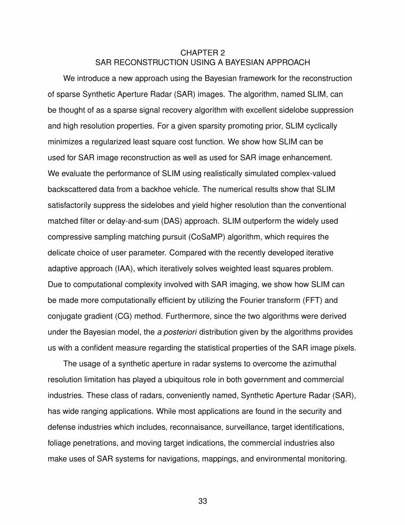
CHAPTER 2SAR RECONSTRUCTION USING A BAYESIAN APPROACH
We introduce a new approach using the Bayesian framework for the reconstruction
of sparse Synthetic Aperture Radar (SAR) images. The algorithm, named SLIM, can
be thought of as a sparse signal recovery algorithm with excellent sidelobe suppression
and high resolution properties. For a given sparsity promoting prior, SLIM cyclically
minimizes a regularized least square cost function. We show how SLIM can be
used for SAR image reconstruction as well as used for SAR image enhancement.
We evaluate the performance of SLIM using realistically simulated complex-valued
backscattered data from a backhoe vehicle. The numerical results show that SLIM
satisfactorily suppress the sidelobes and yield higher resolution than the conventional
matched filter or delay-and-sum (DAS) approach. SLIM outperform the widely used
compressive sampling matching pursuit (CoSaMP) algorithm, which requires the
delicate choice of user parameter. Compared with the recently developed iterative
adaptive approach (IAA), which iteratively solves weighted least squares problem.
Due to computational complexity involved with SAR imaging, we show how SLIM can
be made more computationally efficient by utilizing the Fourier transform (FFT) and
conjugate gradient (CG) method. Furthermore, since the two algorithms were derived
under the Bayesian model, the a posteriori distribution given by the algorithms provides
us with a confident measure regarding the statistical properties of the SAR image pixels.
The usage of a synthetic aperture in radar systems to overcome the azimuthal
resolution limitation has played a ubiquitous role in both government and commercial
industries. These class of radars, conveniently named, Synthetic Aperture Radar (SAR),
has wide ranging applications. While most applications are found in the security and
defense industries which includes, reconnaisance, surveillance, target identifications,
foliage penetrations, and moving target indications, the commercial industries also
make uses of SAR systems for navigations, mappings, and environmental monitoring.
33

At present, satellites imaging (optical) are often used for real time response to
environmental disasters, SAR and its ability to image in all weather conditions offers
a complimentary view of the situations. Using various SAR modes and SAR image
reconstruction techniques certain details and observations can be made that otherwise
would be missed when using optical imaging.
While a significant part of SAR image quality depends on the hardware parameters
of the radar systems, the SAR image construction algorithms plays a pivotal role in
making the most of the collected data. The SAR community has accepted various
methods for SAR image reconstruction, all of which are data-independent approaches,
such as the Fourier Transforms, and backprojection [12]. There are variants improvement
to these basic algorithms via pre and post processes, but the area has been well
developed. The attractiveness of these algorithms are that they are simple to implement
and computationally efficient but they suffer from high sidelobe levels and thus yield low
resolutions. To mitigate this problem we trade its low complexity for higher resolutions.
In this chapter we will focus on data-adaptive approaches for SAR image reconstruction,
with emphasis on algorithms that promotes sparsity in the resulting image. As sparser
images are more beneficial for feature extractions and targets recognitions applications.
Various data-adaptive approaches has been proposed for SAR imaging [13–18].
However, some of these methods, such as Capon [18, 19] and amplitude and phase
estimation(APES) [15, 16] require multiple snapshots to form the sample covariance
matrix. This requirement is hard to satisfy in SAR systems, due to the moving nature of
the platform. Another category of algorithm, the sparse signal recovery algorithms [20–
22], including the popular regularized l1-norm based methods and the greedy-type
approaches, such as compressive sampling matching pursuit (CoSaMP) (see, e.g., [23]
and the references therein), can be used to recover sparse radar images with high
resolution and they do not require multiple snapshots; nevertheless, their performance is
sensitive to user parameters which are hard to choose in practice [24]. In addition, these
34

approaches lack robustness to noise levels, which we will show later in the numerical
examples. One possible data-adaptive algorithm, the iterative adaptive approach
(IAA) [25–28] has been introduced for the SAR imaging application. IAA is robust and
user parameter free and works with few or even a single snapshot. Compared with
the data-independent approaches, IAA is shown to produce images with significantly
reduced sidelobes and much enhanced resolution [29]. However, IAA is computationally
intensive, which to some extent limits its applicability.
We consider a Bayesian-based sparse signal recovery algorithms, named SLIM
(sparse learning via iterative minimization). SLIM is a cyclic algorithm that iteratively
fits the signal to the observation while simultaneously satisfying the sparsity-promoting
constraint. In another perspecive, SLIM is essentially a lb-norm (0 < b ≤ 1) constrained
optimization. It has been shown that in some applications, lb-norm (with b < 1)
constrained optimization outperforms its l1-norm counterparts such as basis pursuit
(BP) [20] and least absolute shrinkage and selection operator (LASSO) [30] in that the
former requires less measurements for reconstruction than the latter [31]. Moreover,
when implemented with fast Fourier transform (FFT) and conjugate gradient (CG), can
yield much faster convergence than many existing SAR imaging algorithms. Compare to
other lb-norm approaches, SLIM has only one user paramter, and it is easy to choose.
One additional benefit, as a Bayesian-type approach, SLIM facilitate the performance
prediction by providing the a posteriori distributions of the reconstructed image pixels.
Furthermore, SLIM have been shown to perform well for MIMO radar imaging [32] so a
natural extension of SLIM is applying it to the case of Synthetic Aperture Radar imaging.
This chapter is structured as follows. In Section II, we introduce the preliminaries
of SAR system and derive the data model for SAR imaging problem. In Section III, we
briefly touch on other data-adaptive algorithms then proceeds to introduce the SLIM
algorithm to the SAR imaging problem and discuss its merits and limitations. In Section
IV, the performance of SLIM is compared with those of two existing SAR imaging
35

Figure 2-1. SAR imaging schematics.
algorithms, namely CoSaMP and IAA, using ideal scatterers as well as the “Backhoe
Data Dome” provided by DARPA IXO and AFRL/SNAS (realistically simulated using
computational electromagnetics software). Finally, we conclude the chapter in Section V.
2.1 Preliminaries and Data Model
In this section, we introduce the principles of SAR imaging, with special emphasis
placed on the geometry of the physical scene and data acquisition mechanism. Based
on the physical interpretation of the data acquisition process, we will apply some
reasonable approximations to derive an appropriate data model, with which various
methods can be applied to form the SAR image.
The data acquisition geometry for spot-light mode SAR is illustrated in Fig. 2-1. A
3-D Cartesian coordinate system is established, centered at the scene patch illuminated
by the radar beam. The non-shaded circle represents a sensor at elevation angle θ and
azimuth angle ϕ. A scatterer in the scene patch located at (x0, y0, z0) is denoted by the
filled circle.
36

In SAR radar system, the antenna transmits an electromagnetic pulse toward the
scene of interest (SOI), and the reflected signal bears the information of the potential
scatterers in the SOI. The time delay τ(x0, y0, z0) of the returned signal associated with a
scatterer located at (x0, y0, z0) is directly determined by the distance R(x0, y0, z0), which
can be calculated as follows:
R(x0, y0, z0) =√
(Rc cos θ cosϕ− x0)2 + (Rc cos θ sinϕ− y0)2+ · · ·
· · · (Rc sinϕ− z0)2
= Rc
√1 + ( x0
Rc)2 + ( y0
Rc)2 + ( z0
Rc)2 − 2 x0
Rccos θ cosϕ− · · ·
· · · 2 y0Rc
cos θ sinϕ− 2 z0Rc
sin θ .
(2–1)
Since the sensor is usually air-borne and the distance Rc is much larger than the
dimension of the scene patch, the expression above can be simplified using the
following approximations:
R(x0, y0, z0) ≈ Rc
√1− 2 x0
Rccos θ cosϕ− 2 y0
Rccos θ sinϕ− 2 z0
Rcsin θ
≈ Rc(1− x0Rc
cos θ cosϕ− y0Rc
cos θ sinϕ− z0Rc
sin θ)
= Rc − (x0 cos θ cosϕ+ y0 cos θ sinϕ+ z0 sin θ) .
(2–2)
The expression in (2–2) gives the distance between the scatterer and the sensor relative
to Rc .
Let p(t) = a(t)e j2πfc t denote the pulse (e.g., a chirp waveform) transmitted toward
the SOI, where a(t) is the complex envelope and fc is the carrier frequency. The
reflected signal r(t, θ,ϕ) can be interpreted as the sum of delayed versions of p(t) with
the amplitudes and phases modified proportionally to the reflectivity g(x , y , z) of the
scatterers. Mathematically, this relation can be expressed as:
r(t, θ,ϕ) =∑x ,y ,z
g(x , y , z)p(t − τ(x , y , z)), (2–3)
37

where τ(x , y , z) = 2R(x ,y ,z)c
and c is the speed of light. With this model, the matched filter
output y(t, θ,ϕ) can be expressed as
y(t, θ,ϕ) =∑x ,y ,z
g(x , y , z)s(t − τ(x , y , z)) + e(t), (2–4)
where s(t) is the auto-correlation function of the transmitted signal p(t) and e(t) is the
additive noise. By taking the Fourier transform of (2–4) and using the relations in (2–2)
above, the phase history data are related to the scatterer reflectivity function by:
Y (f , θ,ϕ) =∑x ,y ,z
g(x , y , z)S(f )e−j2πf2R(x ,y ,z)
c + E(f ) (2–5a)
= C(f )∑x ,y ,z
g(x , y , z)e j4πc(xf cos θ cosϕ+yf cos θ sinϕ+zf sin θ) +
E(f ) (2–5b)
where E(f ) is the Fourier transform of e(t) and C(f ) = S(f )e−j2πf2Rcc is common to all
scatterers in the scene patch so that we will drop it from the expression in the following
discussion for the sake of notational simplicity. Substituting the transformation pairs
u(f , θ,ϕ) = f cos θ cosϕ, v(f , θ,ϕ) = f cos θ sinϕ and w(f , θ,ϕ) = f sin θ into (2–5b), the
output signal can be further written as
Y (f , θ,ϕ) =∑x ,y ,z
g(x , y , z)e j4πc(xu(f ,θ,ϕ)+yv(f ,θ,ϕ)+zw(f ,θ,ϕ)) + E(f ) . (2–6)
With (2–6), the phase history data can thus be interpreted as the 3-D Fourier transforms
of the reflectivity function of the scene patch. In other words, the collected phase history
data form a polar raster in the transformed spatial frequency space.
Consequently, we have a set of samples nonuniformly placed in the spatial
frequency domain. Since there is no fast algorithm for computing Fourier transforms
on a non-Cartesian space, we next seek to reformat the data samples. Basically, the
approaches for this purpose fall into the following two categories: approximation and
interpolation. The approximation-based approach is appropriate when the frequency
38

span �f , the elevation aperture �θ and the azimuth aperture �ϕ are relatively small. In
such a case, we can view the polar grid points as approximately uniform in a Cartesian
cube, which facilitates the application of fast Fourier transforms defined on a Cartesian
coordinate system.
However, for wide-aperture SAR phase history data, the approximation above
is inaccurate. In addition, this method creates technical problems for the 3-D SAR
image fusion application, as is discussed in Section IV. In this situation, we can resort
to the interpolation-based approach to transform the data from the polar coordinate
into the Cartesian coordinate. One particular interpolation-type method involves using
non-uniform fast Fourier transforms (NUFFT) [33]. In this case, the non-uniform data
samples in the 3-D spatial frequency space are first backprojected to the intermediate
image space. Since the image samples are uniform in the 3-D Cartesian coordinate
system, they can be conveniently projected again to the spatial frequency space using
3-D FFT. After this two-step procedure, the data samples in the spatial frequency space
are uniform in the dimensions of u, v , and w .
Based on the scene geometry and the data reformation above, we can derive
the data model as follows. Let M1, M2 and M3 denote the numbers of image grid
points in the x , y and z directions, respectively. Let N1, N2 and N3 denote the number
of frequency grid points, the number of azimuth angle grid points and the number
of elevation angle grid points, respectively. The total number of unknowns is M =
M1 ×M2 ×M3 and the total number of observed data points is N = N1 × N2 × N3. For a
scatterer located at (xj , yk , zl), the N-element steering vector can be written as:
aj ,k,l = [bj ,k,l(1, 1, 1), · · · , bj ,k,l(N1,N2, 1), · · · , bj ,k,l(1, 1,N3), · · · , bj ,k,l(N1,N2,N3)]T ,
1 ≤ j ≤ M1, 1 ≤ k ≤ M2, 1 ≤ l ≤ M3,
(2–7)
39

where bj ,k,l(p, q, r) = e j4πc(upxj+vqyk+wr zl ) for 1 ≤ p ≤ N1, 1 ≤ q ≤ N2 and 1 ≤ r ≤ N3. By
using these definitions, the steering matrix can be written as:
A = [a1,1,1, · · · , aM1,M2,1, · · · , a1,1,M3, · · · , aM1,M2,M3
] . (2–8)
We define s = [g(x1, y1, z1), · · · , g(xM1, yM2
, z1), · · · , g(x1, y1, zM3), · · · , g(xM1
, yM2, zM3
)]T
to be an M × 1 vector containing the reflectivity coefficients, and we stack the observed
data into the vector y. The data model can be compactly expressed in matrix form as:
y = As+ e, (2–9)
where e accounts for the additive noise.
To form SAR images, we essentially need to estimate s from y and A. The
most straightforward method is to perform the inverse Fourier transform, which
gives the conventional delay-and-sum (DAS) or matched filtering approach [34].
In spite of the computational efficiency, the quality of the DAS image is usually
unsatisfactory due to the low resolution and high sidelobes in the image. Compared
with the data-independent DAS method, the data-adaptive approaches, which utilize
the information contained in the data acquired, usually yield better imaging results. In
the following sections, we discuss several data-adaptive algorithms that can be used to
enhance the imaging quality.
2.2 Data-Adaptive Algorithms
In this section, we first review two data-adaptive algorithms, namely CoSaMP and
IAA, as they have the closest ties to SLIM and comment on their performance and
applicability. Then we introduce SLIM and discuss how it can be adapted to the SAR
imaging problem.
2.2.1 Compressed Sampling Matching Pursuit (CoSaMP)
CoSaMP [23] is a sparse signal recovery algorithm, which iteratively identifies
the support of the sparse signal vector and estimates the corresponding entry values.
40

CoSaMP has two user parameters, which determine the sparsity of the estimation
result and the dimension of the potential support. Usually, the signal sparsity is set to
be half of the support dimension, hence we will only give values of the signal sparsity
in the numerical examples. CoSaMP is shown to generate SAR images with higher
resolution than the conventional DAS algorithm [35]. However, the performance of
CoSaMP is highly dependent on the user parameters, whose choice, unfortunately lacks
a clear guidance. Therefore, the performance of CoSaMP can be poor with an improper
selection of the user parameters, which is illustrated later on in the numerical examples.
Furthermore, the performance of CoSaMP degrades as the noise level increases, as
illustrated by the numerical examples.
2.2.2 Iterative Adaptive Approach (IAA)
IAA [25] is a nonparametric adaptive algorithm originally proposed for the array
signal processing application. IAA has been shown to provide much improved
performance over many other data-adaptive algorithms as well as DAS in applications
such as MIMO radar, active sonar, and medical imaging. In a recentwork [29],
IAA is introduced to the SAR imaging problem and it is shown there that IAA can
significantly reduce the sidelobe levels and produce much cleaner images. Though
the performance of IAA is satisfactory, its high computational complexity to some
extent limits its applicability to large dimensional problems. So far, reducing the
computational complexities of IAA is still an open problem. We will discuss further
about the performance of IAA with the numerical examples later on.
2.2.3 Sparse Learning via Iterative Minimization (SLIM)
In this section, we introduce our main algorithm that is based on a Bayesian model.
We named it SLIM (Sparse Learning via Iterative Minimization) since it fits itself to
a given sparse promoting prior iteratively. The SLIM algorithm can be cast into the
41

Bayesian framework by considering the following hierarchical Bayesian model:
y|s, η ∼ CN (As, ηI)
f (s) ∝M
�m=1
e−2b(|sm|b−1)
f (η) ∝ 1,
(2–10)
where η is the noise power and f (s) is a sparsity promoting prior for 0 < b ≤ 1. When
b = 1, the prior becomes the Laplacian prior f (s) ∝ e−2||s||1 which has a finite peak
at 0. When b → 0, the prior becomes f (s) ∝M
�m=1
1|sm|2 , which has an infinite peak at 0.
Therefore, s and η can be estimated using the following MAP approach:
maxs,η
f (y|s, η)f (s) ∝ 1
ηNe− 1
η||y−As||2 M
�m=1
e−2b(|sm|b−1) . (2–11)
This MAP problem is equivalent to the following regularized minimization problem:
mins,η
g(s, η)�= N log η +
1
η||y − As||2 +
M∑m=1
2
b[|sm|b − 1], (2–12)
where 0 < b ≤ 1. Note that the cost function above can be interpreted as the sum of
the negative log-likelihood − log f (y|s, η) and a regularization termM∑
m=1
2b[|sm|b − 1] that
controls the sparsity of s. When b = 1, the regularization term becomes 2||s||1 − 2M,
which is the widely used l1-norm constraint. When b → 0, the regularization term
becomesM∑
m=1
2 log |sm|, which promotes sparsity since, when sm → 0, 2 log |sm| → −∞.
The following cyclic approach is then employed to minimize the cost function at the
i th iteration:
1. Fix the value of η(i−1), and compute the optimal value of s(i) as
s(i) = P(i)AH(AP(i)AH + η(i−1)I)−1y, (2–13)
where P(i) = diag{|s(i−1)1 |2−b, · · · , |s(i−1)
M |2−b}.
2. For a fixed value of s(i), the optimal value of η(i) can be calculated as
η(i) =1
N||y − As(i)||2 . (2–14)
42

SLIM is usually initialized by DAS and terminated when the norm of the difference
between two consecutive estimates of s falls below a pre-specified threshold.
The a posteriori distribution of s can be approximated by the following conditional
probability distribution:
f (s|y, op,
oη) ∝ f (s, y,
op|oη) = f (y|s, o
η)f (s|op)f (op)
∝ exp{− 1
2oη||y − As||2} exp{−1
2sH(
o
P)−1s}
= exp{− 1
2oηyHy + 1
2oηsHAHy + 1
2oηyHAs−
12sH(1o
ηAHA+ (
o
P)−1)s)},
(2–15)
whereop and
oη are the estimated values at convergence. From (2–15), we observe that
the conditional distribution of s given y,op and
oη is a Gaussian distribution. Let µ and �
denote the mean and covariance matrix for this conditional Gaussian random vector, i.e.,
s|y, op,
oη ∼ CN (µ,�). Expanding the expression above and equating the corresponding
terms, we can find:
� =o
P−o
PAH(oηI+ A
o
PAH)−1Ao
P, and µ =o
PAH(Ao
PAH +oηI)−1y . (2–16)
These are the a posteriori mean and covariance matrix of the signal vector s and the
estimate of s is taken to be the a posteriori mean µ. With this a posteriori distribution,
the statistical properties of the estimates can be utilized for performance prediction
purposes for applications such as automatic target recognition.
2.3 Numerical Examples
In this section, we show the SAR imaging capability of SLIM and compare its
performances with those of CoSaMP and IAA as well as the data-independent DAS
algorithm which we will implement via FFT. We first consider a simulated example of
ideal point scatterers, with which imaging properties of the various adaptive algorithms
introduced above are studied. We then examine the imaging capability of the various
algorithms using the realistically simulated “Backhoe Data Dome, Version 1.0” data set.
43

2.3.1 An Example of Ideal Point Scatterers
In this example, the SOI consists of 12 ideal point-like scatterers with uniform
amplitudes 1, denoted by black circles in Figure 2-2(a). Based on the data model in
(2–9), we define
SNR�=
||As||2
||e||2=
||As||2
Nσ2, (2–17)
where σ2 is the average noise power. Throughout this example, the SNR is set to be 10
dB. IAA is set to run for 10 iterations, after which no significant change in image quality
is observed. SLIM and CoSaMP are set to run for 20 iterations.
Figure 2-2(b) shows the SAR image obtained using DAS. Though computationally
efficient, DAS yields an image with high sidelobe levels and poor resolution. Note
that the four closely spaced scatterers in the center of the SOI smear with each other
and appear as one single scatterer. Figures 2-2(d) and (f) show the SAR images
generated by CoSaMP, which has one user parameter that controls the SOI sparsity.
Since this user parameter directly determines the number of non-zero pixels present
in the image and can significantly affect the image quality, the lack of proper guidance
for the choice of this parameter restricts the applicability of this algorithm. As is seen
from Figures 2-2(d) and (g), different values of this user parameter can lead to very
different results, which is undesirable in practice. Figures 2-2(c), (e) and (g) show the
SAR images produced by IAA and SLIM, respectively. As evident from the figures,
IAA and SLIM all possess excellent sidelobe suppression capability, producing clean
images where the presence of the scatterers is clearly indicated and the closely spaced
scatterers are distinguished.
Next, we consider the robustness of the various algorithms against additive noise.
Again by looking at Figure 2-2, with SNR at 10dB, CoSaMP is more sensitive to the
noise level than SLIM and IAA. When the user parameter does not match the scatterer
sparsity, the performance of CoSaMP can be rather poor, as is seen from Figure 2-2(d).
In contrast,SLIM and IAA are all much more robust to the noise level.
44
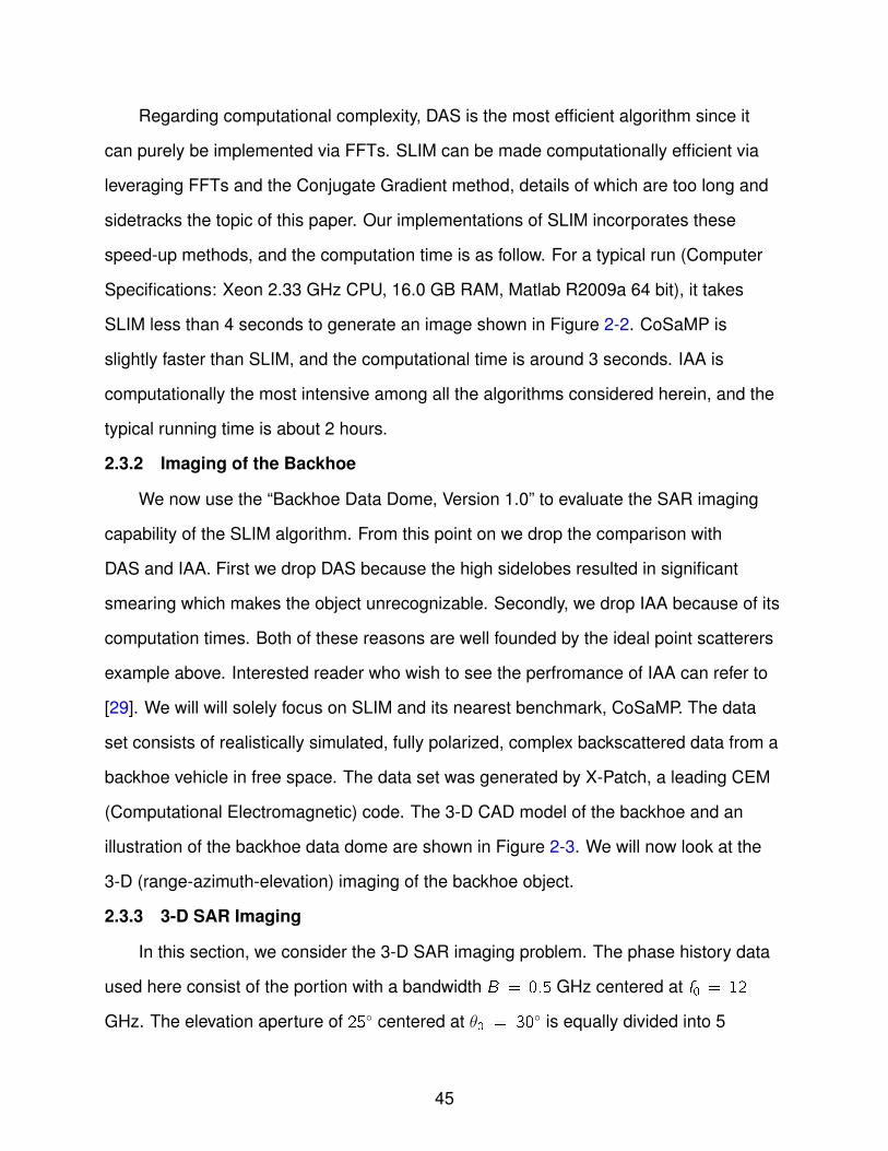
Regarding computational complexity, DAS is the most efficient algorithm since it
can purely be implemented via FFTs. SLIM can be made computationally efficient via
leveraging FFTs and the Conjugate Gradient method, details of which are too long and
sidetracks the topic of this paper. Our implementations of SLIM incorporates these
speed-up methods, and the computation time is as follow. For a typical run (Computer
Specifications: Xeon 2.33 GHz CPU, 16.0 GB RAM, Matlab R2009a 64 bit), it takes
SLIM less than 4 seconds to generate an image shown in Figure 2-2. CoSaMP is
slightly faster than SLIM, and the computational time is around 3 seconds. IAA is
computationally the most intensive among all the algorithms considered herein, and the
typical running time is about 2 hours.
2.3.2 Imaging of the Backhoe
We now use the “Backhoe Data Dome, Version 1.0” to evaluate the SAR imaging
capability of the SLIM algorithm. From this point on we drop the comparison with
DAS and IAA. First we drop DAS because the high sidelobes resulted in significant
smearing which makes the object unrecognizable. Secondly, we drop IAA because of its
computation times. Both of these reasons are well founded by the ideal point scatterers
example above. Interested reader who wish to see the perfromance of IAA can refer to
[29]. We will will solely focus on SLIM and its nearest benchmark, CoSaMP. The data
set consists of realistically simulated, fully polarized, complex backscattered data from a
backhoe vehicle in free space. The data set was generated by X-Patch, a leading CEM
(Computational Electromagnetic) code. The 3-D CAD model of the backhoe and an
illustration of the backhoe data dome are shown in Figure 2-3. We will now look at the
3-D (range-azimuth-elevation) imaging of the backhoe object.
2.3.3 3-D SAR Imaging
In this section, we consider the 3-D SAR imaging problem. The phase history data
used here consist of the portion with a bandwidth B = 0.5 GHz centered at f0 = 12
GHz. The elevation aperture of 25◦ centered at θ0 = 30◦ is equally divided into 5
45

−4 −3 −2 −1 0 1 2 3 4−5
−4
−3
−2
−1
0
1
2
3
4
5
x(meter)
y(m
ete
r)
−15
−10
−5
0
x(meter)
y(m
ete
r)
−4 −3 −2 −1 0 1 2 3 4
−5
−4
−3
−2
−1
0
1
2
3
4
5 −15
−10
−5
0
x(meter)
y(m
ete
r)
−6 −4 −2 0 2 4 6
−5
−4
−3
−2
−1
0
1
2
3
4
5 −15
−10
−5
0
(a) (b) (c)
x(meter)
y(m
ete
r)
−4 −3 −2 −1 0 1 2 3 4
−5
−4
−3
−2
−1
0
1
2
3
4
5 −15
−10
−5
0
x(meter)
y(m
ete
r)
−4 −3 −2 −1 0 1 2 3 4
−5
−4
−3
−2
−1
0
1
2
3
4
5 −15
−10
−5
0
x(meter)
y(m
ete
r)
−4 −3 −2 −1 0 1 2 3 4
−5
−4
−3
−2
−1
0
1
2
3
4
5 −15
−10
−5
0
(d) (e) (f)
x(meter)
y(m
ete
r)
−4 −3 −2 −1 0 1 2 3 4
−5
−4
−3
−2
−1
0
1
2
3
4
5 −15
−10
−5
0
(g)
Figure 2-2. Imaging of Scatterers A) The true scatterer distribution B) DAS. C) IAA. D)CoSaMP (300). E) SLIM (b = 1). F) CoSaMP (12). G) SLIM (b → 0).
non-overlapping subapertures, and the azimuth aperture of 45◦ centered at ϕ0 = 90◦ is
equally divided into 9 non-overlapping subapertures.
We will focus on comparing SLIM with CoSaMP. For CoSaMP, four different values
of the user parameter are considered. The images shown here are projections onto a
2-D plane from a certain azimuth angle. As can be seen from Figure 2-4, SLIM with
b = 1 can produce clean images representing the structure of the backhoe vehicle.
46

(a) (b)
Figure 2-3. Visualizing the Backhoe Data Set A) 3-D CAD model of the backhoe. B) Thebackhoe data dome.
CoSaMP, on the other hand, tends to distort the image with some target features
(such as the line around the -1 elevation) that appear and then disappear as the user
parameter increases.
In Figure 2-5 we show the fused 3-D SAR images of the backhoe vehicle generated
using the SLIM algorithm. We apply NUFFT to interpolate the phase history data
samples onto a uniform 3-D Cartesian grid, which is used for all subapertures. The
fused image is obtained by combining the subimages with the maximum-magnitude
operator as follows:
Image(x , y , z) = max1≤q≤9,1≤r≤5
|Subimage(x , y , z ;ϕq, θr)| . (2–18)
As can be seen from the figure, the images generated are clean and focused, giving
minimum artifacts and nicely showing the imaged vehicle. Moreover, SLIM with either
b → 0 or b = 1 works well in this 3-D fused imaging application.
With the aforementioned numerical examples, the advantages of SLIM over DAS,
IAA and CoSaMP become apparent. First SLIM give results with high fidelity, nicely
indicating the underlying structure of the targets. With the added benefits of a user
parameter that is easy to choose. Furthermore, SLIM is robust to additive noise levels.
In addition, SLIM is computationally efficient and preferable for problems with large data
47

−3−2−10123
−3
−2
−1
0
1
2
3
Range
Ele
va
tio
n
−40
−35
−30
−25
−20
−15
−10
−5
0
−3−2−10123
−3
−2
−1
0
1
2
3
Range
Ele
va
tio
n
−40
−35
−30
−25
−20
−15
−10
−5
0
−3−2−10123
−3
−2
−1
0
1
2
3
Range
Ele
va
tio
n
−40
−35
−30
−25
−20
−15
−10
−5
0
(a) (b) (c)
−3−2−10123
−3
−2
−1
0
1
2
3
Range
Ele
va
tio
n
−40
−35
−30
−25
−20
−15
−10
−5
0
−3−2−10123
−3
−2
−1
0
1
2
3
Range
Ele
va
tio
n
−40
−35
−30
−25
−20
−15
−10
−5
0
−3−2−10123
−3
−2
−1
0
1
2
3
Range
Ele
va
tio
n
−40
−35
−30
−25
−20
−15
−10
−5
0
(d) (e) (f)
Figure 2-4. Backhoe 3-D SAR image reconstruction. A) SLIM (b → 0) B) SLIM (b = 1)C) CoSaMP (128) D) CoSaMP (256) E) CoSaMP (512) F) CoSaMP (1024)
−3 −2 −1 0 1 2 3
−3
−2
−1
0
1
2
3
−40
−35
−30
−25
−20
−15
−10
−5
0
−3 −2 −1 0 1 2 3
−3
−2
−1
0
1
2
3
−40
−35
−30
−25
−20
−15
−10
−5
0
(a) (b)
Figure 2-5. Fused 3-D Image Using SLIM. A) SLIM (q → 0) B) SLIM (q = 1)
sets. The main competing algorithm, CoSaMP, is a good algorithm but since its user
parameter directly ties with the number of non-zeros in the signal space, it requires
some clairvoyant on the side of the user.
48

We have discussed the data acquisition process and data model of SAR imaging
problem. We have introduced a sparse signal recovery algorithm named SLIM to
the SAR imaging application for the purpose of sidelobe suppression and resolution
enhancement. SLIM simply cyclically maximizing the a posteriori probability of the
underlying parameters given the observations. SLIM can also be viewed as the iterative
minimization of the regularized negative log-likelihood function. SLIM is easy to use
(does not require the delicate tuning of user parameters), provides accurate and sparse
signal estimates in a computationally efficient manner, and is robust to additive noise
levels. We have tested the performances of SLIM using various numerical examples. It
provides better resolution than the traditional DAS/FFT approach, it is computationally
more feasible than IAA, and its user parameter, unlike CoSaMP, does not greatly
influence its performance.
49

CHAPTER 3SAR RECONSTRUCTION OF INTERRUPTED DATA
We consider nonparametric adaptive spectral analysis of complex-valued data
sequences with missing samples occurring in arbitrary patterns. We first present
two high-resolution missing-data spectral estimation algorithms: the Iterative Adaptive
Approach (IAA) and the Sparse Learning via Iterative Minimization (SLIM) method.
Both algorithms can significantly improve the spectral estimation performance,
including enhanced resolution and reduced sidelobe levels. Moreover, we consider
fast implementations of these algorithms using the Conjugate Gradient (CG) technique
and the Gohberg-Semencul-type (GS) formula. Our proposed implementations fully
exploit the structure of the steering matrices and maximize the usage of the Fast Fourier
Transform (FFT), resulting in much lower computational complexities as well as much
reduced memory requirements. The effectiveness of the adaptive spectral estimation
algorithms is demonstrated via several numerical examples including both 1-D spectral
estimation and 2-D interrupted synthetic aperture radar (SAR) imaging examples.
Spectral estimation is important in many fields including astronomy, communications,
medical imaging, radar, and underwater acoustics. Most existing spectral estimation
algorithms are devised for uniformly sampled complete-data sequences. However, in
many practical applications, the measured data may be incomplete due, for example,
to sensor failures, outliers, the data compression needs, etc. Missing data problems
are also encountered in modern radar systems. These systems have multiple duties
including searching, tracking and the automatic classification of targets. Switching in
and out of these modes leads to an incomplete phase history data for synthetic aperture
radar (SAR) imaging [36–38]. This loss of the phase history data is also prevalent during
SAR missions encountering high radio frequency (RF) interferences [39, 40].
Many missing-data spectral estimation techniques have been developed previously.
A conceptually and computationally simple method is the matched filter (MF), implemented
50

via using the fast Fourier transform (FFT), with the missing samples set to zero.
However, as a data-independent approach, the FFT approach, as well as its windowed
FFT (WFFT) variations, suffers from poor resolution and high sidelobe level problems.
This high sidelobe level problem is especially severe for the missing data case.
The CLEAN algorithm [41] is used to estimate the spectrum by deconvolving the
missing-data FFT spectrum into the true signal spectrum and the Fourier transform
of the missing pattern windowing function via an iterative approach. Although the
CLEAN algorithm works for both missing and irregularly sampled data sequences, it
cannot resolve closely spaced spectral lines, and hence it may not be a suitable tool for
high-resolution spectral estimation. The multi-taper methods [42, 43] compute spectral
estimates by assuming certain quadratic functions of the available data samples. The
coefficients in the corresponding quadratic functions are optimized according to certain
criteria, but it appears that this type of approaches cannot overcome the resolution limit
of FFT. To achieve high resolution, several parametric algorithms, e.g., those based
on autoregressive (AR) or autoregressive moving-average (ARMA) models, were used
to handle the missing-data problem [44–47]. Although these parametric methods can
provide improved spectral estimates, they are sensitive to model errors.
Several nonparametric adaptive filtering based techniques have been developed
for the missing-data spectral estimation problem [38]. For example, in [48] and [38],
two nonparametric missing-data amplitude and phase estimation (MAPES) algorithms
are derived by using a “maximum likelihood (ML) fitting” criterion. The well-known
expectation maximization (EM) technique [49] is used to solve the estimation problem
iteratively. MAPES works for the general spectral analysis problem with missing samples
occurring in arbitrary patterns. However, MAPES is conceptually complicated and
it is computationally intensive. Furthermore, it is well-known that EM may converge
rather slowly, and, it may even fail to converge globally. As we will show via numerical
51

examples, the spectral estimation performance of MAPES degrades severely in high
data missing ratio cases.
Recently, sparse signal recovery (SSR) techniques (see, e.g., [23] and the
references therein) have attracted much attention in the signal processing community.
Different from the conventional data-adaptive approaches, such as Capon [50] and
APES [51], SSR can work for very few or even one snapshot, and hence can be used
for spectral analysis of irregularly sampled data. However, most of the existing SSR
algorithms, including the well-known CoSaMP (Compressive Sampling Matching
Pursuit) [23], require the bases of the signal components to obey a “restricted isometry
property” [52], which hardly holds in high-resolution spectral estimation problems. As we
will show via numerical examples, CoSaMP fails to work properly in both 1-D spectral
estimation and 2-D interrupted SAR imaging problems.
In this chapter, we will first present two recently-developed high-resolution spectral
estimation algorithms, i.e., the iterative adaptive approach (IAA) [25] and the sparse
learning via iterative minimization (SLIM) method [32, 53]. Both algorithms can work for
both complete and incomplete data samples, and are able to achieve excellent spectral
estimation performance under various conditions. However, both IAA and SLIM are
computationally prohibitive, especially for high-dimensional spectral estimation problems
such as interrupted SAR imaging. We will consider the fast implementation of IAA
for the spectral estimation with missing samples. Moreover, we will propose two fast
implementations of SLIM within the missing-data spectral estimation framework. We will
apply the proposed algorithms to both 1-D spectral estimation and 2-D interrupted
SAR imaging problems. Via several numerical examples, we show that IAA and
SLIM outperform the conventional FFT and MAPES approaches, as well as CoSaMP,
significantly. Compared to the original IAA and SLIM algorithms, the fast implementation
approaches can dramatically reduce the computational complexities and memory
requirements.
52

The remainder of this chapter is organized as follows. Section 3.1 introduces the
IAA and SLIM algorithms. In Section 3.2, we propose three fast missing-data spectral
estimation methods. Several 1-D spectral estimation and 2-D interrupted SAR imaging
examples are presented in Section 3.3. Finally, Section 3.3.2 contains our conclusions.
3.1 Nonparametric Spectral Analysis
In this section, we first present two recently-developed adaptive spectral estimation
algorithms, i.e., IAA and SLIM, within the missing data framework. Both algorithms can
work for 1-D and higher dimensional spectral estimation problems with complete or
incomplete data samples.
3.1.1 Data Model
We consider a spectral estimation problem with M given complex-valued data
samples, and stack the M data samples into an M × 1 column vector x. Let βl (l =
0, 1, · · · ,L − 1) be the complex amplitude at the l th frequency grid point of the
spectrum, and al (l = 0, 1, · · · ,L − 1) be the normalized contribution of the l th
frequency grid point to the M available data samples. Then, the given data samples can
be modeled as follows:
x = Aβ + n, (3–1)
where n denotes the noise vector,
A = [a0, a2, · · · , aL−1] , (3–2)
and
β = [β0, β1, · · · , βL−1]T , (3–3)
with (·)T denoting the transpose. In (3–1), A is referred to as the steering matrix, and
the column vector β represents the spectrum to be estimated. Note that the data model
in (3–1) can be used for both 1-D and higher dimensional spectral estimation problems.
In particular, in the SAR imaging application, β contains the complex-valued reflection
coefficients of scatterers within an imaging area (or volume) of interest. Note also that
53

in high-resolution spectral estimation problems, the grid point number L is usually much
larger than the number of data samples. Hence, the conventional approaches based on
(3–1), such as the maximum likelihood (ML) and least-square (LS) approaches, fail to
work completely.
3.1.2 Iterative Adaptive Approach (IAA)
IAA is an iterative adaptive algorithm based on a nonparametric weighted least
squares (WLS) approach. Let pl = |βl |2 (l = 0, 1, · · · , L − 1) with βk being an
intermediate estimate of βl . The noise and interference covariance matrix l for the l th
frequency grid point can be estimated as:
l =∑k =l
pkakaHk = R− plala
Hl , (3–4)
where (·)H denotes the conjugate transpose,
R =
L−1∑k=0
pkakaHk = Adiag(p)AH , (3–5)
and
p =
[p0 p1 · · · pL−1
]T(3–6)
with diag(·) being a diagonal matrix formed by the elements of a given vector.
Given the noise and interference covariance matrix l , the estimate of βl can be
refined using the WLS criterion as follows:
βl = argmin ∥x− alβl∥2−1
l
, (3–7)
where ∥x∥2
−1
l
= xH−1l x. Solving the optimization problem of (3–7) yields
βl =aHl
−1l x
aHl −1l al
=aHl R
−1x
aHl R−1al
, (3–8)
where we have used (3–4) and the matrix inversion lemma [54].
54
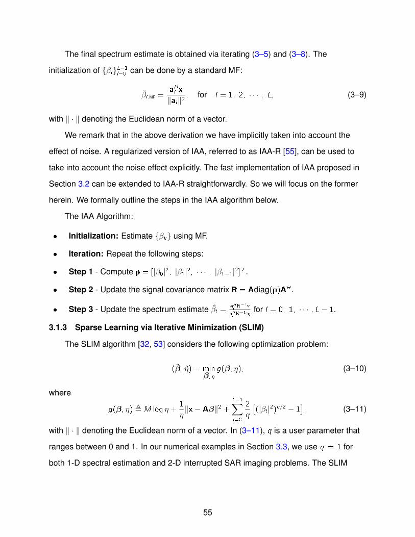
The final spectrum estimate is obtained via iterating (3–5) and (3–8). The
initialization of {βl}L−1l=0 can be done by a standard MF:
βl ,MF =aHl x
∥al∥2, for l = 1, 2, · · · , L, (3–9)
with ∥ · ∥ denoting the Euclidean norm of a vector.
We remark that in the above derivation we have implicitly taken into account the
effect of noise. A regularized version of IAA, referred to as IAA-R [55], can be used to
take into account the noise effect explicitly. The fast implementation of IAA proposed in
Section 3.2 can be extended to IAA-R straightforwardly. So we will focus on the former
herein. We formally outline the steps in the IAA algorithm below.
The IAA Algorithm:
• Initialization: Estimate {βk} using MF.
• Iteration: Repeat the following steps:
• Step 1 - Compute p = [|β0|2, |β1|2, · · · , |βL−1|2]T .
• Step 2 - Update the signal covariance matrix R = Adiag(p)AH .
• Step 3 - Update the spectrum estimate βl =aHlR−1x
aHlR−1al
for l = 0, 1, · · · ,L− 1.
3.1.3 Sparse Learning via Iterative Minimization (SLIM)
The SLIM algorithm [32, 53] considers the following optimization problem:
(β, η) = minβ, η
g(β, η), (3–10)
where
g(β, η) , M log η +1
η∥x− Aβ∥2 +
L−1∑l=0
2
q
[(|βl |2)q/2 − 1
], (3–11)
with ∥ · ∥ denoting the Euclidean norm of a vector. In (3–11), q is a user parameter that
ranges between 0 and 1. In our numerical examples in Section 3.3, we use q = 1 for
both 1-D spectral estimation and 2-D interrupted SAR imaging problems. The SLIM
55

algorithm can be viewed as a maximum a posteriori (MAP) approach with η being the
noise variance and the prior distribution of {βl} being f (βl) ∝ e−2q|βl |q−1.
The optimization problem can be solved iteratively by using the cyclic minimization
(CM) and majorization-minimization (MM) techniques [56]. Let β(t)
and η(t) be
intermediate estimates of β and η, respectively, for the tth iteration. For 0 ≤ q ≤ 1,
2q
[(|βl |2)q/2 − 1
]is a concave function with respect to |βl |2. Hence, the function
2q
[(|βl |2)q/2 − 1
]is majorized by its tangent linear function at |β(t)
l |2, i.e.,
2
q
[(|βl |2)q/2 − 1
]≤ 2
q
[|β(t)
l |q − 1]+
1
p(t)l
[|βl |2 − |β(t)
l |2], (3–12)
where
p(t)l = |β(t)
l |2−q, (3–13)
and the equation holds when |βl | = |β(t)l |. Therefore, we have:
g(β, η) ≤ M log η +1
η∥x− Aβ∥2 +
L−1∑l=0
p(t)l
[|βl |2 − |β(t)
l |2]+
L−1∑l=0
2
q
[|β(t)
l |q − 1]
, h(β, η|β(t)), (3–14)
where, again, the equation holds when |βl | = |β(t)l | for l = 0, 1, · · · , L− 1.
Given η = η(t), minimizing the majorization function of g(β, η), i.e., h(β, η|β(t)), with
respect to β yields:
β(t+1)
=[AHA+ η(t) diag−1
(p(t))]−1
AHx
= diag(p(t))AH�−1x, (3–15)
where
� = Adiag(p(t))AH + η(t)I, (3–16)
and p(t) is defined similarly to p in (3–6), i.e.,
p(t) =∣∣∣β(t)
∣∣∣2−q , [∣∣∣β(t)0
∣∣∣2−q ∣∣∣β(t)1
∣∣∣2−q · · ·∣∣∣β(t)
L−1
∣∣∣2−q]T . (3–17)
56

Furthermore, given β = β(t+1)
, minimizing h(β, η|β(t)) with respect to η yields:
η(t+1) =1
M
∥∥∥x− Aβ(t+1)
∥∥∥2 . (3–18)
The SLIM algorithm estimates β via iterating (3–15), (3–17), and (3–18).
By using the CM and MM properties, we readily have:
g(β(t+1)
, η(t+1))
≤ h(β(t+1)
, η(t+1)|β(t))≤ h
(β(t+1)
, η(t)|β(t))
≤ h(β(t), η(t)|β(t)
)= g
(β(t), η(t)
), (3–19)
i.e., the cost function decreases monotonically.
Again, we initialize {βl}L−1l=0 using MF in (3–9). The variable η is initialized as:
η =1
γL
∥∥∥x− AβMF
∥∥∥2 , (3–20)
where βMF is a column vector formed by {βl ,MF}L−1l=0 similarly to (3–35), and γ is chosen
to be 10 in our numerical examples in Section 3.3. The SLIM algorithm is summarized
below.
The SLIM Algorithm:
• Initialization: Estimate β using MF in (3–9), and set an initial value of η using(3–20).
• Iteration: Repeat the following steps:
• Step 1 - Compute p = |β|2−q.
• Step 2 - Compute � = Adiag(p)AH + ηI.
• Step 3 - Update β = diag(p)AH �−1x.
• Step 4 - Update η = 1M∥x− Aβ∥2.
3.1.4 Computational Complexities and Memory Requirements
For the IAA algorithm, it is computationally intensive to compute the covariance
matrix R in Step 2 and aHl R−1al (for l = 0, 1, · · · , L−1) in Step 3, with the computational
complexities being O(M2L) per iteration. Similarly, SLIM requires O(M2L) flops per
57

iteration to compute � in Step 2. Furthermore, both IAA and SLIM need to pre-compute
and store the steering matrix A of size M × L. Both the computational complexity and
memory requirement of the algorithms, if implemented directly, would be prohibitive,
especially for high-dimensional spectral estimation problems such as SAR imaging,
where M and L could be up to 105 and 107, respectively. We present below several
fast implementations of IAA and SLIM to dramatically reduce their computational
complexities and memory requirements.
3.2 Missing Data Spectral Analysis and Fast Implementations
Hereafter, we focus our discussion on a 2-D spectral estimation problem, since
the interrupted SAR imaging application is of particular interest to us. The 1-D spectral
estimation problem is a special case of its 2-D counterpart. Moreover, our results can be
readily extended to 3- or higher-dimensional spectral estimation problems.
3.2.1 Data Model
We consider the following 2-D spectral estimation problem:
x(m1,m2) =
L1−1∑l1=0
L2−1∑l2=0
βl1,l2zm1l11 zm2l2
2 + n(m1,m2), (3–21)
where
z1 = ej 2πL1 and z2 = e
j 2πL2 . (3–22)
In (3–21), {x(m1,m2)} (m1 = 0, 1, · · · , M1 − 1, and m2 = 0, 1, · · · , M2 − 1)
are the complex-valued data samples, {βl1,l2} (l1 = 0, 1, · · · , L1 − 1, and l2 =
0, 1, · · · , L2 − 1) are the complex amplitudes of signal spectrum at frequency grid
{(l1, l2)}, and {n(m1,m2)} denote the noise.
For notional convenience, we organize the complete data samples {x(m1,m2)} and
the complex-valued amplitudes {βl1,l2} into an M1 ×M2 matrix Xc and an L1 × L2 matrix
58

B, respectively, as follows:
Xc =
x(0, 0) x(0, 1) · · · x(0,M2 − 1)
x(1, 0) x(1, 1) · · · x(1,M2 − 1)
...... . . . ...
x(M1 − 1, 0) x(M1 − 1, 1) · · · x(M1 − 1,M2 − 1)
, (3–23)
and
B =
β0,0 β0,1 · · · β0,L2−1
β1,0 β1,1 · · · β1,L2−1
...... . . . ...
βL1−1,0 βL1−1,1 · · · βL1−1,L2−1
. (3–24)
Then, the complete data model in (3–21) can be rewritten as:
Xc = F1BFT2 +Nc, (3–25)
where Nc is defined similarly to Xc in (3–23) for the noise, and F1 and F2 are M1 × L1
and M2 × L2 inverse Fourier transform matrices, respectively, i.e.,
Fk =
1 1 1 · · · 1
1 zk z2k · · · zLk−1k
1 z2k z4k · · · z2(Lk−1)k
......
... . . . ...
1 zMk−1k z
2(Mk−1)k · · · z
(Mk−1)(Lk−1)k
, for k = 1, 2. (3–26)
By applying the matrix vectorization operator to both sides of (3–25), the complete
data model can be rewritten as:
xc = Fvec(B) + vec(Nc), with F = F2 ⊗ F1 and xc = vec(Xc), (3–27)
where F is the 2-D inverse Fourier transform matrix, vec(·) denotes the vectorization
operator (i.e., stacking the columns of a matrix on top of each other), and ⊗ denotes
59

the Kronecker product of matrices. In (3–27), we have used the fact that vec(ABC) =
(CT ⊗ A)vec(B) (see, e.g., [54]).
Now we assume that only M out of M1M2 samples are available. Let x be an
M × 1 column vector formed by the given data samples, and Jg be the corresponding
M × (M1M2) selection matrix, i.e.,
x = Jg xc. (3–28)
The selection matrix Jg has elements 0 and 1. Each row of the selection matrix contains
one and only one element equal to 1, whose position indicates the selected row/cloumn
index. As an example, let
Jg =
0 1 0 0 0 0
0 0 0 0 1 0
. (3–29)
It can be easily verified that JgC is a 2-row matrix formed by the second and fifth rows
of a 6-row matrix C, while DJTg is a 2-column matrix formed by the second and fifth
columns of a 6-column matrix D. Note also that JTgC expands a 2-row matrix C to a
6-row matrix whose second and fifth rows are equal to the first and second rows of C,
respectively, with the remaining rows being zero. Also, DJg expands a 2-column matrix
D to a 6-column matrix similarly.
From (3–27) and (3–28), we get the data model for the 2-D missing-data spectral
estimation problem:
x =(Jg F
)vec(B) + n. (3–30)
Comparing (3–30) with (3–1), we can see that the aforementioned IAA and SLIM
algorithms in Section 3.1 can be applied to (3–30) directly with the steering matrix
A being Jg F. If implemented directly, the computational complexity and memory
requirement of IAA and SLIM are O(M2L1L2) and O(ML1L2), respectively, which are
prohibitive for practical applications. We present below several computationally efficient
implementations of IAA and SLIM that exploit the structure of JgF.
60

3.2.2 Fast Iterative Adaptive Approach (Fast-IAA)
We present below an efficient implementation of IAA via fully exploiting the structure
of the steering matrix JgF. We refer to this fast implementation of IAA as Fast-IAA.
3.2.2.1 Efficient Computation of the IAA Covariance Matrix
We first consider how to compute the IAA covariance matrix R (step 2 of the IAA
algorithm outline) efficiently.
Let B be an intermediate estimate of B, and P = |B|2 be the corresponding power
estimate, where | · |2 denotes the element-wise modulus-square operation. Then, the IAA
covariance matrix R in (3–5) can be written as:
R =(Jg F
)diag(vec(P))
(Jg F
)H= JgRc JTg, (3–31)
where
Rc = Fdiag(vec(P))FH (3–32)
represents the IAA covariance matrix of the complete data samples corresponding to P.
By using the 2-D inverse Fourier transform property of F, it can be readily verified
that Rc is a Toeplitz-Block-Toeplitz matrix [57], which can be written as follows:
Rc =
R0 RH1 RH
2 · · · RH(M2−1)
R1 R0 RH1 · · · RH
(M2−2)
R2 R1 R0 · · · RH(M2−3)
......
... . . . ...
RM2−1 RM2−2 RM2−3 · · · R0
, (3–33)
61

with
Rm2=
r0,m2r−1,m2
r−2,m2· · · r−(M1−1),m2
r1,m2r0,m2
r−1,m2· · · r−(M1−2),m2
r2,m2r1,m2
r0,m2· · · r−(M1−3),m2
......
... . . . ...
rM1−1,m2rM1−2,m2
rM1−3,m2· · · r0,m2
. (3–34)
In (3–34), rm1,m2(for m1 = −M1 + 1, −M1 + 2, · · · , M1 − 1; and m2 = 0, 1, · · · , M2 − 1)
is the 2-D inverse Fourier transform of P, which can be computed efficiently by using
the 2-D inverse FFT (IFFT) technique. Furthermore, from (3–31), by the selection
matrix property, R is a submatrix of Rc formed by the rows and columns specified by the
selection matrix Jg. By applying 2-D IFFT to P to obtain Rc first and then get R, we can
reduce the computational complexity from O(M2L1L2) to O(L1L2 log(L1L2)).
3.2.2.2 Efficient Computation of B
Now we consider an efficient method to compute B given R. Applying the WLS
method (i.e., (3–8)) to the 2-D spectral estimation data model in (3–30), after some
straightforward manipulations, we readily have:
[B]l1,l2 =cl1,l2dl1,l2
, for l1 = 0, 1, · · · , L1 − 1 and l2 = 0, 1, · · · , L2 − 1, (3–35)
where
cl1,l2 =[Jg F
]H.,l1+M1l2
R−1x
= [F]H.,l1+M1l2
(JTgR
−1x), (3–36)
and
dl1,l2 =[Jg F
]H.,l1+M1l2
R−1[Jg F
].,l1+M1l2
= [F]H.,l1+M1l2
(JTgR
−1Jg)[F].,l1+M1l2, (3–37)
62

with [·]l1,l2 and [·].,l denoting the (l1, l2)th element and the l th column of a given matrix,
respectively.
Given R−1, cl1,l2 in (3–36) can be computed efficiently as follows: (1) compute R−1x;
(2) expand the so-obtained M × 1 vector to an M1M2 × 1 vector by using the selection
matrix property; (3) organize the vector into an M1 ×M2 matrix, and (4) apply 2-D FFT to
the so-obtained M1 ×M2 matrix.
We now consider how to compute dl1,l2 in (3–37) efficiently. Let Q = JTgR−1Jg,
which, obviously, can be obtained from R−1 by inserting some zero rows and columns
specified by the selection matrix JTg. For convenience, we rewrite Q as an M2 ×M2 block
matrix formed by M1 ×M1 sub-matrices, i.e.,
Q =
Q0,0 Q0,1 · · · Q0,M2−1
Q1,0 Q1,1 · · · Q1,M2−1
...... . . . ...
QM1−1,0 QM1−1,1 · · · QM1−1,M2−1
. (3–38)
Then, dl1,l2 can be expressed as a polynomial function of z l11 and z l22 as follows:
dl1,l2 =
M1−1∑m1=−(M1−1)
M2−1∑m2=−(M2−1)
em1,m2z−l1m1
1 z−l2m2
2 , (3–39)
where
em1,m2=
∑M1−1k1=m1
∑M2−1k2=m2
[Qk2,k2−m2]k1,k1−m1
, for m1 ≥ 0 and m2 ≥ 0,∑M1−1+m1
k1=0
∑M2−1k2=m2
[Qk2,k2−m2]k1,k1−m1
, for m1 < 0 and m2 ≥ 0,∑M1−1k1=m1
∑M2−1+m2
k2=0 [Qk2,k2−m2]k1,k1−m1
, for m1 ≥ 0 and m2 < 0,∑M1−1+m1
k1=0
∑M2−1+m2
k2=0 [Qk2,k2−m2]k1,k1−m1
, for m1 < 0 and m2 < 0.
(3–40)
From (3–39), dl1,l2 (for l1 = 0, 1, · · · , L1 − 1 and l2 = 0, 1, · · · , L2 −
1) can be computed efficiently via applying 2-D FFT to the polynomial coefficients
{em1,m2} in (3–40), which reduces the computational complexity from O(M2L1L2) to
O(L1L2 log(L1L2)).
63

The Fast-IAA algorithm is summarized beow.
The Fast-IAA Algorithm:
• Initialization: Apply 2-D FFT to x to get an initial estimate of B.
• Iteration: Repeat the following steps:
• Step 1 - Compute P = |B|2.
• Step 2 - Apply 2-D IFFT to P, and construct the matrix R using (3–33) and 3–34).
• Step 3 - Compute the matrix inverse of R.
• Step 4 - Compute R−1x, and then apply 2-D FFT to JTR−1x to get {cl1,l2}.
• Step 5 - Compute {el1,l2} from R−1 using (3–40).
• Step 6 - Apply 2-D FFT to {el1,l2} to compute {dl1,l2}.
• Step 7 - Update B by using (3–35) and the results of Steps 4 and 6.
Note that the computationally most intensive steps of the Fast-IAA algorithm are the
matrix inverse of R in Step 3 and 2-D FFT/IFFT, with computational complexities O(M3)
and O(L1L2 log(L1L2)), respectively. Hence, the overall computational complexity of the
IAA algorithm is reduced to O(M3) + O(L1L2 log(L1L2)), which is much smaller than
O(M2L1L2) of the original IAA algorithm. We remark that in the complete data case,
R in (3–31) is a Toeplitz-Block-Toeplitz matrix [57], whose inverse can be computed
efficiently by using the Gohberg-Semencul (GS) type formula [58, 59]. We refer to this
GS-type formula based Fast-IAA algorithm as Fast-IAA-GS [60]. The computational
complexity of Fast-IAA-GS is O(L1L2 log(L1L2)). Furthermore, we note that Fast-IAA, as
well as Fast-IAA-GS, does not use the steering matrix explicitly. Hence, it does not need
to pre-compute and store the steering matrix, which significantly reduces the memory
requirement.
3.2.3 Fast SLIM Using Conjugate Gradient (CG-SLIM)
Next, we consider a fast implementation of the SLIM algorithm by using the
conjugate gradient (CG) technique [61]. We refer to this algorithm as CG-SLIM.
64

CG is an efficient method to solve a linear system iteratively. The number of
iterations needed by CG is usually much smaller than the problem size, which can
significantly reduce the computational complexity. In this section, we employ the CG
technique to compute the most intensive step of SLIM, i.e., �−1x. Let
y = �−1x. (3–41)
Then, the unknown vector y in (3–41) can be computed efficiently by using the CG
approach which is outline below.
The Conjugate Gradient Algorithm:
• Initialization: Set an initial vector y, and r0 = r1 = g = x− Ry.
• Iteration: Repeat the following steps until convergence:
• Step 1 - Compute h = �g.
• Step 2 - Compute α = ∥r1∥2gHh
.
• Step 3 - Update y = y + αg.
• Step 4 - Update r0 = r1 and r1 = r1 − αh.
• Step 5 - Update g = r1 +∥r1∥2∥r0∥2g.
For the CG algorithm above, Step 1 is computationally the most intensive, which
involves a matrix-vector product. However, in the 2-D spectral estimation problem
in (3–30), the computational complexity of this step can be reduced by using the
structure of the steering vector. Let B be an intermediate estimate of B, and P = |B|2−q.
Replacing A and p in (3–16) by Jg F and vec(P), respectively, we have:
� =(Jg F
)diag (vec(P))
(Jg F
)H+ ηI
= Jg [Fdiag (vec(P)) F]H JTg + ηI. (3–42)
65

Then, Step 1 of the CG algorithm can be written as:
h =(Jg F
)diag (vec(P))
(Jg F
)Hg+ η g
= JgF[vec(P)⊙
(FH JTgg
)]+ ηg
= F−12d [vec(P)⊙F2d(g)] + η(t)g, (3–43)
where ⊙ denotes the Hadamard product of matrices, and the functions F−12d (·) and
F2d(·) are defined, respectively, as follows:
F−12d (b) = JgFb, (3–44)
and
F2d(g) = FHJTgg. (3–45)
By the properties of the 2-D inverse Fourier transform matrix F and the selection matrix
Jg, (3–44) and (3–45) can be computed efficiently by using the 2-D FFT/IFFT technique.
For the F−12d (·) function in (3–44), we can re-organize the L1L2×1 vector b into an L1×L2
matrix, apply 2-D IFFT to the so-obtained matrix, and then pick up the elements of the
2-D IFFT output specified by the selection matrix to form a column vector. For the F2d(·)
function in (3–45), we can first expand the M × 1 column vector to an M1M2 × 1 vector
via inserting zeros at the positions specified by the selection matrix JTg, re-organize the
vector into an M1 × M2 matrix, and then apply 2-D FFT to the so-obtained matrix. By
using these 2-D FFT and IFFT techniques, the computational complexity of Step 1 of the
Conjugate Gradient algorithm is reduced to O(L1L2 log(L1L2)).
By combining the SLIM algorithm and the CG algorithm, the CG-SLIM algorithm is
summarized below.
The CG-SLIM Algorithm:
• Initialization: Apply 2-D FFT to x to get an initial estimate of B, initialize η, andy = 0.
• Iteration: Repeat the following steps:
66

• Step 1 - Compute P = |B|(2−q).
• Step 2 - Initialize CG using r1 = x−F−12d (vec(P). ∗ F2d(y)) and g = r1.
• Step 3 - Repeat the following steps until ∥r1∥2∥x∥2 ≤ ϵCG:
– Step 3.a - Compute h = F−12d (vec(P). ∗ F2d(g)).
– Step 3.b - Compute α = ∥r1∥2gHh
.
– Step 3.c - Update y = y + αg.
– Step 3.d - Update r0 = r1 and r1 = r1 − αh.
– Step 3.e - Update g = r1 +∥r1∥2∥r0∥2g.
• Step 4 - Update vec(B) = vec(P). ∗ (F2d(y)).
• Step 5 - Update η = 1M
∥∥∥x−F−12d
(vec(B)
)∥∥∥2.We terminate the CG iterations when the ratio of the Euclidean norm of the residue
vector r1 to the Euclidean norm of the data vector x becomes less than a predefined
threshold ϵCG. In the numerical examples in Section 3.3, we choose ϵCG = 10−6. We
note that computationally the most intensive step in the CG-SLIM algorithm is now
2-D FFT/IFFT, with a computational complexity O(L1L2 log(L1L2)). Hence, the overall
computational complexity of CG-SLIM is O(KL1L2 log(L1L2)) per SLIM iteration, with
K being the average CG iteration number, which is usually much smaller than M. For
instance, in the interrupted SAR example in Section 3.3, the data sample number M is
up to 1600, but the CG algorithm usually converges in less than K = 30 iterations.
3.2.4 Fast SLIM Using the Gohberg-Semencul-Type Formula (GS-SLIM)
For a complete-data spectral estimation problem, i.e., when Jg = I, similarly to
Rc in (3–33), the matrix � in (3–42) will be a Toeplitz-Block-Toeplitz matrix [57, 60].
In this case, the vector y = �−1x in (3–41) can be computed efficiently by using the
GS-type formula [58, 59], whose complexity is around min(M31M
22 ,M
21M
32), which is much
lower than O(M21M
22L1L2) of the original SLIM algorithm. Inspired by this, we introduce
below a new fast implementation of SLIM, referred to as GS-SLIM, for the missing data
67

spectral estimation problem. This algorithm includes two steps: (1) estimate missing
samples from an intermediate spectral estimate, and (2) estimate the signal spectrum
from the given data samples, as well as the estimated missing samples. Note that the
second step of the GS-SLIM algorithm is essentially a complete-data spectral estimation
problem, where the aforementioned GS technique can be utilized.
For the 2-D spectral estimation problem in (3–30), the SLIM formulation in (3–10)
and (3–11) can be written as follows:
(B, η) = minB, η
g(B, η), (3–46)
where
g(B, η) , M log η +1
η∥x− JgFvec(B)∥2 +
L1−1∑l1=0
L2−1∑l2=0
2
q
[(|βl1,l2 |2)q/2 − 1
]. (3–47)
Below, we employ the maximization-minimization (MM) technique to solve the
optimization problem iteratively.
Let xm and Jm be the missing samples and the associated selection matrix,
respectively. Let B(t) and η(t) be the intermediate estimates of B and η at the tth
iteration, respectively. Naturally, the missing data can be estimated as follows:
x(t)
m = JmFvec(B(t)). (3–48)
We consider below an efficient method to update the B and η estimates such that the
cost function in (3–47) decreases monotonically.
68

From (3–47), we readily have:
g(B, η) = M log η +1
η∥x− JgFvec(B)∥2 +
L1−1∑l1=0
L2−1∑l2=0
2
q
[(|βl1,l2 |2)q/2 − 1
](3–49)
≤ M log η +1
η∥x− JgF vec(B)∥2 + 1
η∥x(t)m − JmFvec(B)∥2
+
L1−1∑l1=0
L2−1∑l2=0
2
q
[(|βl1,l2|2)q/2 − 1
](3–50)
= M log η +1
η∥x(t)c − Fvec(B)∥2 +
L1−1∑l1=0
L2−1∑l2=0
2
q
[(|βl1,l2|2)q/2 − 1
](3–51)
≤ M log η +1
η∥x(t)c − Fvec(B)∥2 +
L1−1∑l1=0
L2−1∑l2=0
p(t)l1,l2
[|βl1,l2|2 − |βt
l1,l2|2]+
L1−1∑l1=0
L2−1∑l2=0
2
q
[|β(t)
l1,l2|q − 1
](3–52)
, h(B, η|B(t), x(t)
c ), (3–53)
where x(t)c is the complete data composed by the estimated missing sample vector x(t)m,
as well as the given sample vector x. The inequality in (3–52) is obtained similarly to
(3–14), and
p(t)l1,l2
= |β(t)l1,l2
|2−q. (3–54)
Obviously, the equality in g(B, η) ≤ h(B, η|B(t), x(t)
c ) holds when B = B(t). In other
words, the function g(B, η) is majorized by h(B, η|B(t), x(t)
c ) at the point B = B(t).
Therefore, we can obtain the estimates of B and η via minimizing h(B, η|B(t), x(t)
c ) with
respect to B and η.
Similarly to (3–15), given η = η(t), minimizing h(B, η|B(t), x(t)
c ) with respect to B,
yields:
vec(B(t+1)) = vec(P(t))⊙(FH�−1
c x(t)
c), (3–55)
where
�c = Fdiag(
vec(P(t)))FH + η(t)I. (3–56)
69

As discussed above, �c is a Toeplitze-Block-Toeplitz matrix [57, 60] having the form:
�c =
�0 �H1 �H
2 · · · �H(M2−1)
�1 �0 �H1 · · · �H
(M2−2)
�2 �1 �0 · · · �(M2 − 3)H
......
... . . . ...
�M2−1 �M2−2 �M2−3 · · · �0
, (3–57)
and
�m2=
σ0,m2σ−1,m2
σ−2,m2· · · σ−(M1−1),m2
σ1,m2σ0,m2
σ−1,m2· · · σ−(M1−2),m2
σ2,m2σ1,m2
σ0,m2· · · σ−(M1−3),m2
......
... . . . ...
σM1−1,m2σM1−2,m2
σM1−3,m2· · · σ0,m2
+ ηδ(m2)I, (3–58)
where δ(m2) is a Kronecker delta function, and {σm1,m2} is the 2-D Fourier transform
of P and can be computed efficiently by using 2-D FFT. Furthermore, via exploiting the
Toeplitze-Block-Toeplitz structure of �c, �−1xc in (3–55) can be computed efficiently by
using the generalized GS algorithm [57, 60].
On the other hand, given B = B(t+1), minimizing h(B, η|B(t), x(t)
c ) with respect to η
yields:
~η =1
M
∥∥∥x(t)c − Fvec(B(t+1)
)∣∣∣2 . (3–59)
Equation (3–59) is a natural estimate of η given B = B(t+1). However, we find empirically
that the GS-SLIM algorithm suffers from a slow convergence problem using (3–59).
Instead, we propose to update η as follows:
η(t+1) = ρ~η + (1− ρ)η(t) =ρ
M
∥∥∥x(t)c − Fvec(B(t+1)
)∥∥∥2 + (1− ρ)η(t), (3–60)
where ρ is choose to be the given-to-complete data ratio, i.e., ρ = MM1M2
, in the numerical
examples in Section 3.3.
70

The 2-D spectrum B is estimated via iterating (3–48), (3–55), (3–57) and (3–60).
We prove below that the cost function g(B, η) decreases monotonically. First, we readily
have the first-order derivative of h(B(t+1), η|B(t), x(t)
c ) as follows:
∂h(B(t+1), η|B(t), x(t)
c )
∂η=
M
η−
∥∥∥x(t)c − Fvec(B(t+1)
)∥∥∥2η2
=M
η2(η − ~η), (3–61)
where ~η is defined in (3–59). From (3–61), we can see that∂h(B(t+1),η|B(t),x
(t)
m,η(t))
∂η< 0
for 0 < η < ~η and∂h(B(t+1),η|B(t),x
(t)
m,η(t))
∂η> 0 for η > ~η. In other words, the function
h(B(t+1), η|B(t), x(t)
m , η(t)) monotonically decreases with respect to η for 0 < η < ~η, and
monotonically increases for η > ~η. On the other hand, obviously we have η(t) ≤ η(t+1) ≤
~η when η(t) ≤ ~η, and ~η ≤ η(t+1) ≤ η(t) when η(t) > ~η. That immediately implies:
h(B(t+1), η(t+1)|B(t), x(t)
c ) ≤ h(B(t+1), η(t)|B(t), x(t)
c ). (3–62)
Using (3–62) and the fact that h(B, η)|B(t), x(t)
c ) majorizes g(B, η) (see (3–53)), we
immediately have:
g(B(t+1), ηt+1) ≤ h(B(t+1), η(t+1)|B(t), x(t)
c )
≤ h(B(t+1), η(t)|B(t), x(t)
c )
≤ h(B(t), η(t)|B(t), x(t)
c ) = g(B(t), η(t)), (3–63)
i.e., the cost function g(B, η) is monotonically decreasing. The GS-SLIM algorithm is
summarized below.
The GS-SLIM Algorithm:
• Initialization: Set an initial value for η, let xm = 0, and apply 2-D FFT to x to getan initial estimate of B.Iteration: Repeat the following steps:
• Step 1 - Compute P = |B|(2−q).
71

• Step 2 - Apply 2-D FFT to P to compute �c in (3–57) and (3–58).
• Step 3 - Compute y = �−1c xc using the generalized GS algorithm.
• Step 4 - Update vec(B) = vec(P)⊙F2d(y).
• Step 5 - Compute ~xc = F−12d (vec(B)).
• Step 6 - Update η = ρ~η + (1− ρ)η with ~η = 1M∥xc − ~xc∥2.
• Step 7 - Update missing data estimate xm = Jm~xc and the associated completedata xc.
3.3 Numerical Examples
We present below several 1-D spectral estimation and 2-D interrupted SAR imaging
examples to demonstrate the performance of the missing data spectral estimation
algorithms and their fast implementations.
3.3.1 1-D Spectral Estimation
To demonstrate the performance improvements of the new missing data spectral
analysis approaches over some existing ones, we first consider a simple example in
Figure 3-1. The complete data has 128 samples, and contains 8 complex sinusoids.
The frequencies and amplitudes of the sinusoids are indicated by circles in Figure 3-1.
The data is corrupted by a zero-mean circularly symmetric complex white Gaussian
noise with variance σ20 = 0.001. In Figures 3-1(a)-3-1(e), we provide the spectra
estimates obtained by windowed FFT (WFFT), APES/MAPES, CoSaMP, IAA and
SLIM, respectively. A Taylor window with a −30 dB sidelobe level is used for WFFT.
The iteration numbers for all iterative approaches, including MAPES, CoSaMP, IAA,
and SLIM, are fixed to 20. (In our examples, we did not find significant performance
improvement after 20 iterations for all algorithms.) We choose the user parameter of
CoSaMP to be 32. For SLIM, we choose q = 1. The subplots at the left, middle and right
columns in Figure 3-1 show the results obtained from the complete data, 50% and 30%
data, respectively. The available data samples are selected randomly. For Figure 3-1(b),
we use APES for the complete data case, and MAPES for the two missing data cases.
72

From Figure 3-1(a), it is clear that WFFT suffers from the low resolution and high
sidelobe level problems. The sidelobe level increases significantly in the missing data
case. Due to the high sidelobe levels, several targets fail to be detected. In Figure
3-1(b), APES provides a good spectral estimation performance for the complete
data case. Its missing data variant, i.e., MAPES, behaves well when 50% of the data
samples are available. However, its performance degrades significantly when the
available data percentage decreases to 30%. Moreover, MAPES is computationally
very intensive. The computation times needed by MAPES, when implemented on an
ordinary personal computer (Intel Xeon CPU at 2.67 GHz; 12 GB RAM), for the two
missing-data examples in Figure 3-1(b) are 969 and 847 seconds, respectively, while
the computation times needed by all the other algorithms are less than 1 second. We
can also see in Figure 3-1(c) that CoSaMP produces many false peaks in the missing
data cases. From Figures 3-1(d) and 3-1(e), we note that both IAA and SLIM provide
good spectral estimation performance under various conditions. All of the 8 sinusoids
can be identified clearly even with only 30% data samples available. We remark that
the amplitude estimates of SLIM are significantly biased downward. However, with the
correctly identified sinusoidal number and frequencies, the amplitude estimates can
be refined readily using, for example, the standard least-squares (LS) method or the
RELAX algorithm [62].
We next consider a more challenging problem of analyzing a long data sequence
where 800 out of 1000 data samples are available for spectral estimation. The data
sequence contains 100 complex-valued sinusoids, and is corrupted by a zero-mean
circularly symmetric complex white Gaussian noise with variance σ20 = 0.001.
Figures 3-2(a)-3-2(f) show the spectral estimates (zoomed-in to show details within
the [0.21, 0.24] Hz band) obtained by WFFT, IAA, SLIM, Fast-IAA, CG-SLIM, and
GS-SLIM, respectively. Again, the data-adaptive algorithms outperform the conventional
data-independent WFFT approach significantly. The performance of the fast implementations
73

0 0.2 0.4 0.6 0.8 1−60
−50
−40
−30
−20
−10
0
10
Frequency
Ampli
tude (
dB)
Length=128; rho=1; WFFT; runTime=0s
0 0.2 0.4 0.6 0.8 1−60
−50
−40
−30
−20
−10
0
10
Frequency
Ampli
tude (
dB)
Length=128; rho=0.5; WFFT; runTime=0s
0 0.2 0.4 0.6 0.8 1−60
−50
−40
−30
−20
−10
0
10
Frequency
Ampli
tude (
dB)
Length=128; rho=0.3; WFFT; runTime=0s
(a)
0 0.2 0.4 0.6 0.8 1−60
−50
−40
−30
−20
−10
0
10
Frequency
Ampli
tude (
dB)
Length=128; rho=1; APES; runTime=0.02s
0 0.2 0.4 0.6 0.8 1−60
−50
−40
−30
−20
−10
0
10
Frequency
Ampli
tude (
dB)
Length=128; rho=0.5; MAPES; runTime=968.73s
0 0.2 0.4 0.6 0.8 1−60
−50
−40
−30
−20
−10
0
10
Frequency
Ampli
tude (
dB)
Length=128; rho=0.3; MAPES; runTime=847.18s
(b)
0 0.2 0.4 0.6 0.8 1−60
−50
−40
−30
−20
−10
0
10
Frequency
Ampli
tude (
dB)
Length=128; rho=1; CoSaMP; runTime=0.09s
0 0.2 0.4 0.6 0.8 1−60
−50
−40
−30
−20
−10
0
10
Frequency
Ampli
tude (
dB)
Length=128; rho=0.5; CoSaMP; runTime=0.08s
0 0.2 0.4 0.6 0.8 1−60
−50
−40
−30
−20
−10
0
10
Frequency
Ampli
tude (
dB)
Length=128; rho=0.3; CoSaMP; runTime=0.07s
(c)
0 0.2 0.4 0.6 0.8 1−60
−50
−40
−30
−20
−10
0
10
Frequency
Ampli
tude (
dB)
Length=128; rho=1; IAA; runTime=0.42s
0 0.2 0.4 0.6 0.8 1−60
−50
−40
−30
−20
−10
0
10
Frequency
Ampli
tude (
dB)
Length=128; rho=0.5; IAA; runTime=0.15s
0 0.2 0.4 0.6 0.8 1−60
−50
−40
−30
−20
−10
0
10
Frequency
Ampli
tude (
dB)
Length=128; rho=0.3; IAA; runTime=0.07s
(d)
0 0.2 0.4 0.6 0.8 1−60
−50
−40
−30
−20
−10
0
10
Frequency
Ampli
tude (
dB)
Length=128; rho=1; SLIM; runTime=0.24s
0 0.2 0.4 0.6 0.8 1−60
−50
−40
−30
−20
−10
0
10
Frequency
Ampli
tude (
dB)
Length=128; rho=0.5; SLIM; runTime=0.08s
0 0.2 0.4 0.6 0.8 1−60
−50
−40
−30
−20
−10
0
10
Frequency
Ampli
tude (
dB)
Length=128; rho=0.3; SLIM; runTime=0.05s
(e)
Figure 3-1. Nonparametric spectral estimation without and with missing samples, wherethe complete data length is 128. The subplots in the left, middle and rightcolumns are obtained with the complete data, 50% data, and 30% data,respectively. A) WFFT B) MAPES C) CoSaMP D) IAA E) SLIM
74

0.21 0.215 0.22 0.225 0.23 0.235 0.24−60
−50
−40
−30
−20
−10
0
10
Frequency
Ampli
tude (
dB)
Length=1000; rho=0.8; WFFT; runTime=0.04s
0.21 0.215 0.22 0.225 0.23 0.235 0.24−60
−50
−40
−30
−20
−10
0
10
Frequency
Ampli
tude (
dB)
Length=1000; rho=0.8; SLIM; runTime=44.34s
(a) (d)
0.21 0.215 0.22 0.225 0.23 0.235 0.24−60
−50
−40
−30
−20
−10
0
10
Frequency
Ampli
tude (
dB)
Length=1000; rho=0.8; IAA; runTime=84.98s
0.21 0.215 0.22 0.225 0.23 0.235 0.24−60
−50
−40
−30
−20
−10
0
10
Frequency
Ampli
tude (
dB)
Length=1000; rho=0.8; CG−SLIM; runTime=0.4s
(b) (e)
0.21 0.215 0.22 0.225 0.23 0.235 0.24−60
−50
−40
−30
−20
−10
0
10
Frequency
Ampli
tude (
dB)
Length=1000; rho=0.8; Fast−IAA; runTime=8.39s
0.21 0.215 0.22 0.225 0.23 0.235 0.24−60
−50
−40
−30
−20
−10
0
10
Frequency
Ampli
tude (
dB)
Length=1000; rho=0.8; GS−SLIM; runTime=1.4s
(c) (f)
Figure 3-2. Nonparametric spectral estimates for data sequences with missing sampleswhen 800 out of 1000 data samples are available for spectral analysis. A)WFFT B) IAA C) Fast-IAA D) SLIM E) CG-SLIM F) GS-SLIM
of IAA and SLIM are very close to those of their original algorithms. From Figure 3-2, we
see again that the amplitude estimates of SLIM and its variants are biased downward,
while IAA and its variant provide rather accurate amplitude estimates.
The missing data samples can be recovered by simply applying FFT (see Equation
(3–48)) to the spectral estimates of SLIM or its fast implementations. The missing-data
IAA (MIAA) algorithm in [63] can also be used to recover the missing samples from
the IAA or Fast-IAA spectra estimates, which, however, is more complicated both
conceptually and computationally than its SLIM counterpart. Figures 3-3(a) and 3-3(b)
75

0 20 40 60 80 100−15
−10
−5
0
5
10
15
TruthEst.
0 20 40 60 80 100−15
−10
−5
0
5
10
15
TruthEst.
(a)
0 20 40 60 80 100−15
−10
−5
0
5
10
15
TruthEst.
0 20 40 60 80 100−15
−10
−5
0
5
10
15
TruthEst.
(b)
Figure 3-3. Missing samples estimation by SLIM, the subplots in the left and rightcolumns represent the real and imaginary parts of the data samples,respectively. A) CG-SLIM B) GS-SLIM
show the missing samples estimated by CG-SLIM and GS-SLIM, respectively. As
we can see, the missing samples can be estimated quite accurately. To mitigate the
biased amplitude estimation problem of CG-SLIM and GS-SLIM, we can apply the
efficient complete-data IAA algorithm discussed in Section 3.2.2, i.e., Fast-IAA-GS, to
the estimated missing samples obtained using the SLIM variants, as well as the given
samples. We refer to these two new spectral estimation procedures (i.e., CG-SLIM
followed by Fast-IAA-GS, and GS-SLIM followed by Fast-IAA-GS) as CG-SLIM-IAA
and GS-SLIM-IAA, respectively. Note that due to the usage of the GS-type formula,
Fast-IAA-GS is computationally quite efficient. Furthermore, the Fast-IAA-GS step
can be initialized by using the CG-SLIM or GS-SLIM spectral estimate to reduce the
needed number of iterations. Figures 3-4(a) and 3-4(b) show the spectral estimates
obtained by CG-SLIM-IAA and GS-SLIM-IAA, respectively. The Fast-IAA-GS iteration
number is set to be 5 for both algorithms. From Figures 3-4(a) and 3-4(b), we can see
that CG-SLIM-IAA and GS-SLIM-IAA provide more accurate amplitude estimates than
CG-SLIM and GS-SLIM. In particular, comparing Figures 3-2(c) and 3-4(a), we see
76

that CG-SLIM-IAA provides a similar spectral estimate as Fast-IAA. However, as we will
show below, CG-SLIM-IAA is computationally much more efficient than Fast-IAA.
0.21 0.215 0.22 0.225 0.23 0.235 0.24−60
−50
−40
−30
−20
−10
0
10
Frequency
Ampli
tude (
dB)
Length=1000; rho=0.8; CG−SLIM−IAA; runTime=0.78s
0.21 0.215 0.22 0.225 0.23 0.235 0.24−60
−50
−40
−30
−20
−10
0
10
Frequency
Ampli
tude (
dB)
Length=1000; rho=0.8; GS−SLIM−IAA; runTime=1.75s
(a) (d)
Figure 3-4. Nonparametric spectral estimates for data sequences with missing sampleswhen 800 out of 1000 data samples are available for spectral analysis. A)CG-SLIM-IAA B) GS-SLIM-IAA
The computation times needed by the 1-D spectral estimation methods to obtain
Figures 3-2 and 3-4 are shown in Table 3-1. Clearly, the proposed fast implementations
of IAA and SLIM are computationally much more efficient than their original counterparts.
In particular, the proposed CG-SLIM and GS-SLIM algorithms reduce the computation
times needed by SLIM from 44.34 seconds to 0.4 and 1.4 seconds, respectively. The
computational efficiencies of CG-SLIM-IAA and GS-SLIM-IAA are close to those of
CG-SLIM and GS-SLIM, respectively. In particular, CG-SLIM-IAA needs only 0.78
seconds, which amount to only 9.3% of the computation time needed by Fast-IAA (8.39
seconds, while providing a similar spectral estimation performance to Fast-IAA. Although
for this 1-D spectral estimation example, CG-SLIM is computationally more efficient
than GS-SLIM, as we will show in Section 3.3.2, GS-SLIM can be computationally more
efficient than CG-SLIM for 2-D interrupted SAR imaging.
Table 3-1. Computation times needed by IAA, SLIM and their fast implementations.Alg. WFFT IAA SLIM Fast-
IAACG-SLIM
GS-SLIM
CG-SLIM-IAA
GS-SLIM-IAA
Time (s) 0.04 84.98 44.34 8.39 0.4 1.4 0.78 1.75
77

3.3.2 2-D Interrupted SAR Imaging
In the following examples, we illustrate the applications of the missing-data spectral
analysis algorithms to interrupted SAR imaging using incomplete phase history data.
WFFT, ρ: 100%, t:0.53s
−35
−30
−25
−20
−15
−10
−5
0
(a) (b)
Figure 3-5. Slicy object and benchmark SAR image A) Photograph of the object (takenat 45◦ azimuth angle). B) benchmark SAR image formed with a 288× 288(not 40× 40) data matrix.
We use the two-dimensional phase-history data of an object called Slicy generated
at 0◦ azimuth angle using XPATCH [64], a high frequency electromagnetic scattering
prediction code for complex 3-D objects. A photo of the Slicy object taken at 45◦ azimuth
angle and a SAR image benchmark obtained from a complete 288× 288 data matrix are
shown in Figures 3-5(a) and 3-5(b), respectively. Below, we use only a 40 × 40 center
block of the phase-history data for SAR imaging.
Figures 3-6 - 3-8 show the SAR images obtained from the 40 × 40 complete data,
and two randomly interrupted data. The available data patterns for the two interruption
cases are shown in Figures 3-7(a) and 3-8(a), where the available data ratios are 68%
and 30%, respectively. We provide the SAR images obtained by IAA, SLIM, and their
fast variants, i.e., Fast-IAA/Fast-IAA-GS, CG-SLIM and GS-SLIM, as well as WFFT and
CoSaMP. Note that we use Fast-IAA-GS for the complete data case in Figure 3-6, and
Fast-IAA for the two missing data cases in Figures 3-7 and 3-8. Again, the iteration
numbers for all iterative approaches, including CoSaMP, IAA, and SLIM, are all fixed to
78

10. We set the CoSaMP user parameter to be 3000, the SLIM parameter q = 1, and
ϵCG = 10−6 for CG-SLIM. The noise variance estimate η of SLIM is initialized using
(3–20).
Figures 3-6(b), 3-7(b) and 3-8(b) show the SAR images formed by WFFT, where
a 2-D Taylor window with a −30 dB sidelobe level is applied. Again, WFFT has low
resolution and high sidelobe problems, especially for the interrupted scenarios. The
object features are smeared under the interrupted data conditions. We can also see
that the CoSaMP approach fails to work properly under all conditions. IAA, SLIM, and
their fast variants, i.e., Fast-IAA, CG-SLIM and GS-SLIM, significantly improve the
interrupted SAR imaging quality, in terms of both higher imaging resolution and lower
sidelobe levels, as evidenced by sharper SAR images with less ghost artifacts. In this
example, SLIM and its variants provide the best imaging performance, as compared to
the benchmark in Figure 3-5 for all interruption conditions. Note that only 0.56% of the
data samples was used to form the SAR images in Figure 3-8, compared to the entire
288× 288 data samples in Figure 3-5.
Table 3-2 provides the computation times needed by the aforementioned algorithms
under various interruption conditions. Again, the proposed fast implementation
approaches have significantly enhanced computational efficiencies. In particular, for
the interruption example in Figure 3-7, GS-SLIM needs only 2.4 seconds, which amount
to only 0.4% of the computation time needed by SLIM (584.1 seconds).
Table 3-2. Computation times needed by IAA, SLIM and their fast implementations forinterrupted SAR imaging under various interruption conditions.
Alg. WFFT CoSaMP IAA SLIM Fast-IAA-GS CG-SLIM GS-SLIMFig. 3-6 (s) 0.01 173.0 11933 9260 2.63 7.08 1.87Fig. 3-7 (s) 0.32 192.5 1119 584 12.90 6.50 2.40Fig. 3-8 (s) 0.03 163.7 240 131 3.80 4.10 1.80
We have considered using data-adaptive methods, namely IAA and SLIM, for
spectral estimation of data sequences with missing samples. Both methods can provide
significantly improved spectral estimates, in terms of spectral resolution and lower
79

5 10 15 20 25 30 35 40
5
10
15
20
25
30
35
40 CoSaMP, ρ: 100%, t:173.12s
−35
−30
−25
−20
−15
−10
−5
0
(a) (e)WFFT, ρ: 100%, t:0.01s
−35
−30
−25
−20
−15
−10
−5
0SLIM, ρ: 100%, t:9260.684s
−35
−30
−25
−20
−15
−10
−5
0
(b) (f)IAA, ρ: 100%, t:11933.079s
−35
−30
−25
−20
−15
−10
−5
0CG−SLIM, ρ: 100%, t:7.082s
−35
−30
−25
−20
−15
−10
−5
0
(c) (g)Fast−IAA−GS, ρ: 100%, t:2.632s
−35
−30
−25
−20
−15
−10
−5
0GS−SLIM, ρ: 100%, t:1.87s
−35
−30
−25
−20
−15
−10
−5
0
(d) (h)
Figure 3-6. Modulus of the SAR images of the Slicy object obtained from a 40× 40complete data matrix. A) Available data pattern. B) WFFT C) IAA D)Fast-IAA-GS E) CoSaMP F) SLIM G) CG-SLIM H) GS-SLIM
80

5 10 15 20 25 30 35 40
5
10
15
20
25
30
35
40 CoSaMP, ρ: 68%, t:192.504s
−35
−30
−25
−20
−15
−10
−5
0
(a) (e)WFFT, ρ: 68%, t:0.323s
−35
−30
−25
−20
−15
−10
−5
0SLIM, ρ: 68%, t:584.062s
−35
−30
−25
−20
−15
−10
−5
0
(b) (f)IAA, ρ: 68%, t:1119.768s
−35
−30
−25
−20
−15
−10
−5
0CG−SLIM, ρ: 68%, t:6.523s
−35
−30
−25
−20
−15
−10
−5
0
(c) (g)Fast−IAA, ρ: 68%, t:12.907s
−35
−30
−25
−20
−15
−10
−5
0GS−SLIM, ρ: 68%, t:2.395s
−35
−30
−25
−20
−15
−10
−5
0
(d) (h)
Figure 3-7. Modulus of the interrupted SAR images of the Slicy object under a randominterruption condition (68% data available compared to Figure 3-6). A)Available data pattern. B) WFFT C) IAA D) Fast-IAA E) CoSaMP F) SLIM G)CG-SLIM H) GS-SLIM
81
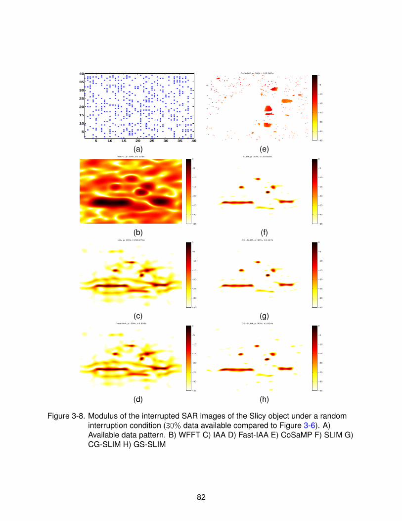
5 10 15 20 25 30 35 40
5
10
15
20
25
30
35
40 CoSaMP, ρ: 30%, t:163.693s
−35
−30
−25
−20
−15
−10
−5
0
(a) (e)WFFT, ρ: 30%, t:0.025s
−35
−30
−25
−20
−15
−10
−5
0SLIM, ρ: 30%, t:130.605s
−35
−30
−25
−20
−15
−10
−5
0
(b) (f)IAA, ρ: 30%, t:239.874s
−35
−30
−25
−20
−15
−10
−5
0CG−SLIM, ρ: 30%, t:4.147s
−35
−30
−25
−20
−15
−10
−5
0
(c) (g)Fast−IAA, ρ: 30%, t:3.836s
−35
−30
−25
−20
−15
−10
−5
0GS−SLIM, ρ: 30%, t:1.824s
−35
−30
−25
−20
−15
−10
−5
0
(d) (h)
Figure 3-8. Modulus of the interrupted SAR images of the Slicy object under a randominterruption condition (30% data available compared to Figure 3-6). A)Available data pattern. B) WFFT C) IAA D) Fast-IAA E) CoSaMP F) SLIM G)CG-SLIM H) GS-SLIM
82

sidelobe levels, as compared to the conventional data-independent approaches. We
have introduced several fast implementations of these algorithms, namely Fast-IAA,
CG-SLIM and GS-SLIM, by exploiting the structures of the steering matrices and
maximizing the utility of FFTs. Via several numerical examples of both 1-D spectral
analysis and 2-D interrupted SAR imaging, we have demonstrate the effectiveness of
IAA and SLIM for spectral estimation and the computational efficiencies of their fast
implementations.
83

CHAPTER 4SAR GROUND MOVING TARGET INDICATION
Synthetic aperture radar (SAR) imaging has been widely used in many civilian
and military applications [12, 65]. Since SAR was originally developed for imaging
the stationary scene, a moving target is usually misplaced due to the motion-induced
Doppler-shift in the SAR image [66–69]. The goal of SAR-based ground moving target
indication (GMTI) is twofold: detection of moving targets in the SAR images, and
parameter estimation, including velocity and location determination of the moving
targets. This problem is rather challenging when the moving targets are slow and small
and are buried in strong stationary ground clutter.
GMTI techniques have been developed for most of the recent history of radar
systems. GMTI can be performed incoherently with a single channel SAR [70, 71], or
coherently with a two- or multi-channel SAR [72–75]. Techniques such as displaced
phase center antenna (DPCA) and along-track interferometry (ATI) have been widely
used in the surveillance community [74, 76–78]. The traditional data-independent DPCA
and ATI investigations are mostly limited to two-channel SAR. Multi-channel DPCA and
ATI have been presented recently [79–81]. However, they may fail to work properly for
challenging GMTI problems, such as for small moving target detection in the presence of
strong stationary clutter. With the availability of increased computational power, adaptive
SAR based GMTI can make up for the shortcomings of conventional SAR based GMTI
methods. Via adaptively forming angle-Doppler images, moving targets can be detected
effectively from ground clutter via space-time adaptive processing (STAP) [82, 83].
STAP can significantly improve the low-velocity and small target detection capability
in the presence of strong clutter and jamming interferences. However, it is well-known
that conventional STAP has a high computational requirement [82, 83]. Moreover, it
needs a large amount of target-free homogeneous secondary data, which is hardly
available in practice [82, 83]. An l1-norm based method, which belongs to the category
84

of compressive sensing (CS) algorithms, is used for STAP in [84]. However, the CS
algorithms usually require user-parameters, which are not easy to tune, and have rather
high computational cost.
In this chapter, new moving target indication techniques for multi-channel airborne
SAR are presented. Via adaptively forming the velocity versus cross-range images
for each range bin of interest, small moving targets can be detected effectively even
in the presence of strong stationary ground clutter. An iterative adaptive approach
(IAA) [25, 55] is used to form velocity versus cross-range images for each range
bin of interest. This weighted least squares based IAA algorithm is robust and user
parameter free. IAA can provide better performance than DPCA and ATI, while having
much lower computational requirement than conventional STAP and obviating the
need of homogeneous target-free secondary data. The performances of the proposed
algorithms are demonstrated using the Air Force Research Laboratory (AFRL) Gotcha
airborne SAR based GMTI data set [85].
The remainder of this chapter is organized as follows. In Section 4.1, we introduce
the SAR imaging geometry and the data model of this SAR based GMTI problem. We
then discuss the need for array calibrations in Section 4.2. We present our approach
to both calibrate the antenna gains and determine the array inter-element spacings.
Stationary clutter cancelation, target detection and velocity estimation algorithms are
presented in Section 4.3. In Section 4.4, we discuss the AFRL Gotcha GMTI data
set and present several examples to demonstrate the performance of the proposed
algorithms. Finally, concluding remarks are given.
4.1 Geometry and Data Model
We consider the 3-D geometry of an airborne SAR system as shown in Figure
4-1. The airplane moves with a velocity vp along the y direction. There are M receive
channels placed along the flight path, and the distance between the mth antenna and the
first antenna is denoted as Lm. Hence L1 = 0. Assume that a moving target in the k th
85

Vehicle
vt
Antenna 1
Antenna m
L m
vp
y
x
z
Flight
path
θ
B
C
A
Figure 4-1. Geometry of an airbore multi-channel SAR system.
range bin with radial velocity vt is at the angle θ relative to the normal of the synthetic
aperture, as shown in Figure 4-1. The angle between the radial velocity of the target and
the slant range line BC in Figure 4-1 is denoted as ϕ. Then, after range compression,
the received data due to the moving target for the mth antenna and the nth probing pulse
can be modeled as:
ym(k , n) = gmbej2π
[2vp
λfPRFsin(θ)+
2vtλfPRF
cos(ϕ)]ne j2π
Lmλ
sin(θ), (4–1)
m = 1, 2, ... ,M, k = 1, 2, ... ,K , n = 1, 2, ... ,N, (4–2)
where gm is the antenna gain of the mth antenna relative to the first antenna (and hence
g1 = 1), b is the complex-valued response from the moving target, λ is the wavelength
of the radar, and fPRF is the pulse repetition frequency (PRF). In (4–2), e j2π2vp
λfPRFn sin(θ)
denotes the phase delay due to the motion of the platform, e j2π2vt
λfPRFn cos(ϕ) denotes the
phase delay due to the motion of the moving target, and e j2πLmλ
sin(θ) denotes the phase
delay due to the antenna distance Lm. By letting
fd =2vpλfPRF
, (4–3)
86

fv =2vtλfPRF
cos(ϕ), (4–4)
and
lm =Lm
λ, (4–5)
we have
ym(k , n) = gmbej2π[fd sin(θ)+fv ]ne j2πlm sin(θ). (4–6)
Let
ft = fd sin(θ) + fv (4–7)
denote the total Doppler caused by both platform and target motions, and let
ηm =lm
fd. (4–8)
Then we can rewrite ym(k , n) as
ym(k , n) = gmbej2πft(n+ηm)e−j2πfvηm . (4–9)
Note that we have fv = 0 for the stationary ground clutter, ηm can be uniformly or
non-uniformly spaced depending on the array geometry, and η1 = L1/fd = 0.
For each m, applying the discrete-time Fourier transform along n to (4–9), we get
the SAR image for the mth antenna:
zm(k , s) = gmbe−j2πfvηme j2πfsηmγ(fs − ft), s = 1, 2, ... ,N, (4–10)
where fs = (s − 1)/N is the normalized Doppler frequency for the s th Doppler bin (or
cross-range bin), and
γ(fs − ft) =sin[πN(fs − ft)]
sin[π(fs − ft)]e−j(N−1)π(fs−ft). (4–11)
87

When the distances and relative gains among the antennas are known, the gains and
the second phase shift term in Equation (4–10) can be compensated out as follows:
~zm(k , s) =e−j2πfsηm
gmzm(k , s) = be−j2πfvηmγ(fs − ft). (4–12)
Because fv = 0 for the stationary ground clutter, the data model in the presence of the
stationary ground clutter and noise can be written as:
~zm(k , s) = be−j2πfvηmγ(fs − ft) +∑s ′
cs′γ(fs − f cs′ ) + em(fs), (4–13)
where f cs′ is the Doppler shift of the stationary or ground clutter, cs′ is the complex-valued
response of the clutter in the s ′th Doppler bin, and em(f ) is the noise term. Stacking
{~zm(k , s)}Mm=1 into a vector ~z(k , s), we have:
~z(k , s) = a(fv)bγ(fs − ft) + a(0)∑s′
cs′γ(fs − f cs′ ) + e(fs), (4–14)
where
~z(k , s) = [ ~z1(k , s) ~z2(k , s) · · · ~zM(k , s) ]T , (4–15)
and
a(fv) = [ 1 e−j2πfvη2 · · · e−j2πfvηM ]T , (4–16)
is the steering vector.
Our problem of interest is to detect the moving target and estimate its velocity from
~z(k , s).
4.2 Array Calibration
For applications that rely on accurate phase histories, array calibration is crucial [86,
87]. For our data model, this means having correct values for the antenna inter-element
spacing, Lm, and the individual antenna gain, gm. Even with prior knowledge of the array
geometry and the antenna specifications, array calibration is still necessary. Depending
88

on the physical array configurations and platform geometry, in-situ antenna performance
is never the same as its free-space counterparts.
4.2.1 Distances Among Antennas
The antenna inter-element spacing may be unknown in practice. We consider
estimating the spacings using the Rank-1 method [86] in this subsection. Consider the
estimation of the distance between Antennas 1 and 2. For a given Doppler bin s, we
have (in the absence of noise):
z1,2(k , s) =
z1(k , s)
z2(k , s)
=
1
g2ejπ s−1
N
L2D
z1(k , s),k = 1, · · · , K , (4–17)
where D = vp/fPRF is the distance the radar traveled within a pulse repetition interval
(PRI). In the derivation of (4–17), we dropped the term e j2πfvηm in (4–10) by assuming
fv = 0, since the target power is negligible compared to the stationary ground clutter
power. For each Doppler bin s, the ideal (noiseless) covariance matrix for z1,2(k , s) is
R1,2(s) = E{z1,2(k , s)zH1,2(k , s)}
= p(s)a1,2(s)aH1,2(s), s = 1, · · · , N, (4–18)
where p(s) =∑K
k=1 |z1(k , s)|2 is the power of z1(k , s) (k = 1, · · · , K ), and
a1,2(s) =[1 g2e
jπ s−1N
L2D
]T(4–19)
is the steering vector. Note that, a1,2(s)aH1,2(s) is a 2 × 2 Rank-1 matrix. Note also that
the steering vector contains the variable L2. The steering vector can be estimated from
the eigen-decomposition of the covariance matrix R1,2(s), which is usually replaced
by the sample covariance matrix [88] in practice. Then the antenna separation can be
determined from the estimated steering vector. More details can be found in references
89

[86]. This process can be repeated for each antenna element to determine all of the
inter-element distances of the array.
4.2.2 Antenna Gains
To estimate the gains of the individual antenna element (relative to the first
antenna), we follow a similar regime. With the estimated antenna distances, the
phase delay due to this distance can be compensated out. We assume a constant
gain across all Doppler bins, but a varying gain as a function of range bin. We found that
this assumption helps improve the GMTI performance for our applications. For a fixed
range bin k (k = 1, · · · , K ), we consider the following data model (in the absence of
noise):
�z(k , s) =
z1(k , s)
z2(k , s) · e−jπs−1N
L2D
...
zM(k , s) · e−jπ s−1N
LMD
=
1
g2(k)
...
gM(k)
z1(k , s), s = 1, · · · , N, (4–20)
where M is the number of array elements. The ideal (noiseless) covariance matrix is
�R(k) = E{�z(k , s)�zH(k , s)}
= �p(k)�a(k)�aH(k), k = 1, · · · , K , (4–21)
where �p(k) =∑N
s=1 |z1(k , s)|2 is the power of z1(k , s) (s = 1, · · · , N), and
�a(k) = [1 g2(k) · · · gM(k)]T (4–22)
90

is the steering vector at the k th range bin. Note that, �a(k)�aH(k) is also a Rank-1 matrix.
Again, the sample covariance matrix �R(k) is used to replace the covariance matrix �R(k)
in practice, where
�R(k) =1
N
N∑s=1
�z(k , s)�zH(k , s), k = 1, · · · , K . (4–23)
Let
�R(k) =
M∑i=1
�λi(k)�ei(k)�eHi (k) (4–24)
denote the eigen-decomposition of �R(k), and let
�e1(k) = [�e11(k), �e12(k), · · · , �e1M(k)]T (4–25)
be the eigenvector corresponding to the largest eigenvalue. Then the estimation of the
steering vector �a(k) can be written as
�a(k) =
[1�e12(k)
�e11(k)· · · �e1M(k)
�e11(k)
]T, (4–26)
and the mth antenna gain at the range bin k is estimated as:
gm(k) =�e1m(k)
�e11(k), m = 2, · · · , M. (4–27)
4.3 Ground Moving Target Indication (GMTI)
After antenna calibration, our goal is to detect the moving target and to estimate fv
(the Doppler shift induced by the motion of the moving target) and ft (the total Doppler
shift which includes both the location information in the cross-range dimension and the
velocity) of the moving target. Once we have fv and ft , the true location fd of the moving
target in the Doppler dimension can be calculated by using Equation (4–7). We estimate
the value of b at all possible fv values for each pixel in the SAR image domain. The peak
values and the corresponding peak locations of these images can be used to indicate
91

the presence of the moving target and the associated target parameter estimates, fv and
ft , of fv and ft .
4.3.1 Ground Clutter Cancelation Using RELAX
The detection of weak moving targets in urban environments can be challenging
due to the strong response of the stationary ground clutter such as buildings, trees,
and other reflective structures. This problem is exacerbated by the Doppler induced
displacement of the moving targets onto existing strong stationary ground return, such
as return from a building. The removal of stationary ground clutter would then improve
the probability of correctly separating the moving targets from the background.
We consider the following stationary clutter rejection approach to address this
challenging problem by using the RELAX algorithm [62, 89]. By taking the stationary
ground clutter and a moving target into consideration, the data model in Equation (4–14)
can be rewritten as:
~z = a(fv)~b + a(0)~c + ~e, (4–28)
where ~z = ~z(k , s), ~b = bγ(fs − ft) and ~c =∑
s′ cs ′ γ(fs − f cs′ ) are, respectively, the
complex-valued responses of the moving targets and stationary clutter at the given
normalized Doppler frequency f , and ~e = e(fs) is the noise term. For notational
convenience, we have omitted the dependence of ~y, ~b, ~c , and ~e on k and s.
By applying the nonlinear least-squares (NLS) criterion, ~c as well as the ~b and fv
can be estimated by minimizing the following cost function:
F [~c , ~b, fv ] =∥∥∥~z− a(fv)~b − a(0)~c
∥∥∥2 , (4–29)
where ∥ · ∥ denotes the Frobenius norm. The optimization problem can be solved by
using the RELAX algorithm [62, 89] as follows.
For a given estimated ~c (the mean value of ~z can be used as the initial value of ~c in
practice), let
~zb = ~z− a(0)~c . (4–30)
92

Then, the cost function of (4–29) can be simplified as
Fb[~b, fv ] =∥∥∥~zHb − a(fv)~b
∥∥∥2 . (4–31)
Minimizing (4–31) with respect to ~b and fv yields:
~b =aH(fv)~zb
M
∣∣∣∣fv=fv
, (4–32)
where M is the antenna number, and
fv = argminfv
∥∥∥∥[I− a(fv)aH(fv)
N
]~zb
∥∥∥∥2= argmax
fv|aH(fv)~zb|2. (4–33)
The cost function in (4–33) can be computed by applying DTFT (discrete-time Fourier
transform) to ~zb. On the other hand, given the estimated fv and ~b, ~c can be re-estimated
by minimizing the cost function
Fc [~c ] = ∥~yc − a(0)~c∥2, (4–34)
where
~zc = ~z− a(fv)~b. (4–35)
Solving this optimization problem yields:
~c =aH(0)~zc
M. (4–36)
Therefore, the original NLS problem can be solved via iterating (4–32), (4–33) and
(4–36) until convergence. The steps of the RELAX algorithm are illustrated below.
The RELAX Algorithm:
• Initialize ~c = aH(0)~zM
• Iterate:
– Step 1:~zb = ~z− a(0)~c
93

fv = argmaxfv |aH(fv)~zb|2~b = aH(fv )~zb
M
∣∣∣fv=fv
– Step 2:~zc = ~z− a(fv)~b
~c = aH(0)~zcM
• until convergence or a certain number of iterations is reached
After ~c is estimated, the stationary clutter can be removed using Equation (4–30).
In this RELAX algorithm, we have fixed the steering vector of the stationary clutter
as a(0). In practice, because of various errors and perturbations, the true steering vector
of the ground clutter may not be exactly a(0). RELAX can still be used to remove a
significant portion of the ground clutter as long as its steering vector is close to a(0).
After using RELAX to remove a major portion of the stationary ground clutter, we use
the robust non-parametric IAA algorithm for moving target detection and target velocity
estimation.
4.3.2 Moving Target Detection Using IAA
Since we have used RELAX to estimate the intensity of the stationary clutter return,
we can subtract it out from ~z, as shown in Equation (4–30), to get
~zb = a(fv)~b + �e, (4–37)
where �e includes the residual of the ground clutter and noise.
The goal now is to detect moving targets. The recently proposed IAA algorithm [25,
55] is considered herein to make an estimate of ~b = [~b1, · · · , ~bN ]T , where ~bi = ~b(fvi)
(i = 1, · · · , N) are the responses at different potential velocities, and fvi (i = 1, · · · , N)
are scanning points of fv . IAA has also been presented in Chapter 2, interested readers
should follow the reference for a detailed development of IAA. Let
A = [a1, · · · , aN ] (4–38)
94

denote the steering matrix, where ai = a(fvi), we have the following compact data model:
~zb = A~b+ �e. (4–39)
IAA solves for ~b by using a weighted least squares approach, which involves the
minimization of the following cost function,
min~bi
∥~zb − ~biai∥2~Q−1i
, i = 1, · · · , N, (4–40)
where ∥u∥2~Q−1 , uH ~Q−1u. In Equation (5–21), the interference and noise covariance
matrix ~Qi is given by:
~Qi = ~R− |~bi |2aiaHi , (4–41)
where
~R =
N∑i=1
|~bi |2aiaHi (4–42)
is the IAA covariance matrix. By letting ~P denote an N × N diagonal matrix whose
diagonal contains the signal power as ~pi = |~bi |2, we can rewrite Equation (5–23) in the
following matrix form:
~R = A~PAH . (4–43)
The minimization of Equation (5–21) with respect to ~bi gives:
~bi =aHi
~Q−1i ~zb
aHi~Q−1i ai
. (4–44)
Using the definition of ~Qi and the matrix inversion lemma, Equation (5–25) can be
written as [25]:
~bi =aHi
~R−1~zb
aHi~R−1ai
, (4–45)
which avoids the computation of ~Q−1i for each i = 1, · · · , N, and significantly saves the
computation time. Since the a priori knowledge of ~P is required in Equation (5–24) to
calculate the covariance matrix ~R, IAA needs to be implemented iteratively. Usually, IAA
is initialized with the periodogram.
95

Once ~b is estimated by IAA, the moving target will be detected based on the peak
value of ~b, the estimate of ~b. The elements, whose fv are near zero, inside ~b will be
removed from ~b to further reduce the effect of the residue stationary ground clutter.
Then the peak value of ~b is compared with a threshold, and a moving target will be
indicated if the peak value is greater than the threshold. Moreover, the fv corresponding
to the peak value of ~b can be used to estimate the radial velocity of the target. The radial
velocity of the moving target can be calculated from (4–4) as:
vt =λfPRF
2 cos(ϕ)fv (meters/second). (4–46)
Note that ϕ can be determined from the flight information of the platform when collecting
the data.
The flow chart of the entire processing chain for the proposed adaptive SAR based
GMTI is given in Figure 4-2.
Ran
ge a
nd c
ross
-ran
ge
com
pres
sion
Cha
nnel
Cal
ibra
tion
Gro
und
clut
ter
canc
ella
tion
us
ing
RE
LA
X
IAA
Mov
ing
targ
ets
dete
ctio
n an
d m
otio
n pa
ram
eter
s es
timat
ion
SAR image for channel 1
SAR image for channel 2
SAR image for channel M
Calibrated data for channel 1
Calibrated data for channel 2
Calibrated data for channel M
Stationary clutter removed data for
channel 1
Stationary clutter removed data for
channel 2
Stationary clutter removed data for
channel M
Velocity v.s. cross-range
image
Antenna 1
Antenna M
Antenna 2
Figure 4-2. The flow chart of the entire processing chain for the proposed adaptive SARbased GMTI.
4.4 Analysis of the AFRL GOTCHA Data Set
4.4.1 Description of the AFRL Gotcha GMTI Data Set
To demonstrate the effectiveness of our approach, we apply it to the AFRL Gotcha
open data set [85]. This data set is an airborne X-band SAR data collected in an urban
environment. Three phase-history sets, all with HH polarization corresponding to three
different channels, are contained in this data set. The carrier frequency used in this
96

system is 9.6 GHz, the probing signal is a linear frequency modulated (LFM) signal with
a bandwidth of 640 MHz, and the PRF is 2171.6 Hz.
02000
40006000
−4000
−2000
0
2000
0
2000
4000
6000
x (meter)y (meter)
z (m
eter
)
Vehicle
Airplane
(a)
0 1000 2000 3000 4000 5000 6000 7000
−4000
−3000
−2000
−1000
0
1000
2000
3000
x (meter)
y (m
eter
)
Vehicle
Airplane
(b)
Figure 4-3. AFRL Gotcha data scene setup. A) 3D view. B) 2D view.
The data collection duration is about 71 seconds. There are multiple vehicles
moving on the roads near buildings in the scene under interrogation. The ground truth
of one of the moving vehicles is provided in the data set. The locations of the radar
platform and the vehicle of interest, which is referred to as the target vehicle, are given
in the auxiliary data of the AFRL data set. The tracks of the radar platform and the
target vehicle during the 71-second duration are plotted in Figure 4-3. The vehicle is
moving away from the radar platform, which induces a negative Doppler-shift. There are
a total of 5400 original range bins in the data set, but only 384 range bins, range-gated
97

to center around the target vehicle, are provided in the data set. The diagram of the
range-gating is shown in Figure 2 of the reference [85].
4.4.2 SAR Imaging
We begin the data processing by forming the SAR images. Due to the truncation
of the data set for distribution purposes, the 384 range bins given by this data set are
centered around the moving target vehicle. These range bins are not aligned, as shown
in Figure 3 of the reference [85]. Fortunately, the offset value for each probing pulse
was given in the data set. So the first step after we load the data is to shift the range
bins and align them. A simple 2D FFT of the aligned data can give a reasonable SAR
image, as shown in Figure 4-4(a) at the 46th second for a CPI of 1 second for one of
the 3 channels. However, the image is smeared because of the high sidelobe problem
of FFT. To reduce the sidelobes and hence smearing, before the 2D FFT, a 2D Taylor
window with parameter 4 and -80 dB sidelobe level is applied to the data, followed by
zero padding. The resulting SAR image with Taylor windowing and zero padding is
shown in Figure 4-4(b). However, the range migration induced by the target motion will
cause coupling between the range and cross-range dimensions and this smears the
image of the moving target. The Keystone transform method [90, 91] is used to reformat
the SAR data, correct the range migration, and image the moving target. The resulting
SAR image is shown in Figure 4-4(c), with the imaging quality visibly enhanced.
4.4.3 Array Calibration
The Gotcha SAR based GMTI system has three antennas, but unfortunately, the
information about the antenna array is not provided in the data set. So we calibrated the
array by estimating the distances among the antennas and their corresponding gains
(relative to the first antenna) from the data set using the approach presented in Section
4.2. The estimated distances between antennas for the entire 71 seconds are shown in
Figure 4-5. It is shown in this figure that the distance estimates are stable and almost
98

Normalized Cross−Range
SAR at 46 seconds
−0.4 −0.3 −0.2 −0.1 0 0.1 0.2 0.3 0.4 0.5−60
−50
−40
−30
−20
−10
0dB
(a)
Normalized Cross−Range
SAR at 46 seconds
−0.4 −0.3 −0.2 −0.1 0 0.1 0.2 0.3 0.4 0.5
−50
−40
−30
−20
−10
0dB
(b)
Normalized Cross−Range
SAR at 46 seconds
−0.4 −0.3 −0.2 −0.1 0 0.1 0.2 0.3 0.4 0.5
−50
−40
−30
−20
−10
0
(c)
Figure 4-4. SAR images using data at the 46th second. A) 2D FFT only. B) 2D FFT with2D Taylor window and zero padding. C) 2D FFT with 2D Taylor window, zeropadding and Keystone reformatting.
constant over time. From Figure 4-5, the estimated distance between Antennas 1 and 2
is around 0.238 meters, and between Antennas 1 and 3 is 0.476 meters.
4.4.4 Velocity Ambiguity Analysis
Equations (4–46) shows that for a given fv , the estimated target velocity is
dependent on the wavelength and the PRF. Table 4-1 shows various fv values and
the corresponding velocities for the AFRL Gotcha data set, where the wavelength is
λ = 0.0312 meters, and the PRF is fPRF = 2171.6 Hz.
However, because of the large inter-antenna spacing, velocity ambiguity problems
exist. To better understand the ambiguity problem, we consider the spectral window
99

0 10 20 30 40 50 60 700.2
0.25
0.3
0.35
0.4
0.45
0.5
Time (second)
Dis
tan
ce (
met
er)
Distance between antenna 1 and 2Distance between antenna 1 and 3
Figure 4-5. Estimated distance between Antennas.
fv Velocity (meters/second) Velocity (miles/hour)0.1 3.3925 7.63320.2 6.7850 15.26640.3 10.1776 22.89950.4 13.5701 30.53270.5 16.9626 38.16590.6 20.3551 45.79910.7 23.7477 53.43230.8 27.1402 61.06540.9 30.5327 68.69861.0 33.9252 76.3318
Table 4-1. Target velocity versus fv .
defined as [92]
W (f ) =
∣∣∣∣∣M∑
m=1
e j2πf ηm
∣∣∣∣∣2
. (4–47)
For the AFRL Gotcha GMTI data set at the 46th second, we have η1 = 0, η2 = 4.952,
and η3 = 9.904. The spectral window with f ∈ [−0.5, 0.5] is plotted in Figure 4-6. It is
clearly shown that the peak repetition occurs at a period of around 0.2. We define the
maximal frequency without ambiguity as fmax, which means that there are no ambiguity
within f ∈ [−fmax, fmax]. From Figure 4-6, we find that fmax = 0.101, which corresponds
to the vehicle velocity of about 3.425 meters/second (based on Table 4-1), which is far
below a normal vehicle speed on the road. For a fixed number of receive channels, the
inter-antenna spacing is constrained by two opposing factors. On the one hand, large
100

−0.5 0 0.5
2
4
6
8
Spectral window
Normalized frequency, fv
Figure 4-6. Spectral windows for the array geometry of the AFRL Gotcha GMTI system.
inter-antenna spacing increases vehicle velocity estimation accuracy and resolution as
a result of longer aperture. On the other hand, to avoid velocity ambiguity problems, the
inter-antenna spacing should be small.
The above analysis shows that because of the limitations of the AFRL Gotcha GMTI
data set, the unambiguous velocity range is much smaller than the velocity range of a
normal moving vehicle. We will suggest later on some methods to resolve the ambiguity
problem based on scene context.
4.4.5 Adaptive GMTI
The center range bin of the AFRL Gotcha GMTI data set at the 46th second is used
to evaluate our approach first, because the ground truth of the target vehicle is known.
For comparison purposes, the results of DPCA and ATI are also presented. Because
DPCA and ATI investigations so far are limited to two-channel SAR, only the data of
Antennas 1 and 2 are used for all methods. At the 46th second, the vehicle of interest,
a Durango, is located at the center range bin, and the ground truth of the vehicle is
known. This vehicle is moving away from the radar platform, which induces a negative
Doppler-shift. For all the SAR images in this section, we use circles to indicate the
uncorrected locations of the detected moving targets. The multiple potential corrected
locations (caused by the ambiguity problem discussed above) of the moving targets
are marked by triangles “△” and “∇”, with the directions of the triangles indicating the
leaving or closing of the targets.
101

We plot the DPCA output in the complex plane in Figure 4-7(a), and the SAR image
with detected targets in Figure 4-7(b). We see that the traditional DPCA fails to identify
the mover and falsely identify two non-movers. The output of ATI is given in Figure
4-8(a), and the corresponding SAR image with detected targets in Figure 4-8(b). The
ATI technique is able to find the mover, but also gives two false alarms. The GMTI
results of the proposed adaptive approach are given in Figure 4-9. Figure 4-9(a) shows
the velocity versus normalized cross-range image of IAA. In this image, the locations
and values of the peaks indicate the presence of the moving target and the associated
target parameter estimates. The SAR image with the detected moving targets is shown
in Figure 4-9(b). It can be seen that the mover was identified correctly without any false
alarm by using the adaptive approach. However, the mover velocity cannot be uniquely
determined due to the velocity ambiguity problem caused by the large inter-antenna
spacing. As shown in Figure 4-9(a), there are more than one peak in this velocity versus
normalized cross-range image. We next attempt to find the correct peak location of the
target vehicle by shifting the target vehicle to its potential original locations based on
the estimated possible velocities. The potential original locations are discarded if they
are outside the range [−0.25, 0.25], which is the range of the normalized cross-range
of the SAR image. The results are shown in Figure 4-9(c), where two potential original
locations of the vehicle are denoted by the triangle, and the true location of the vehicle
is also given in this SAR image. The right triangle matches the true location and is close
to a road. Based on the scene context of the SAR image, we can discard the left triangle
because it is not close to a road [93].
In the second example, we consider the scenario at the 46th second again, but data
from all three antennas at all range bins are processed by IAA. The SAR image with
IAA detected moving targets is shown in Figure 4-10. Multiple targets, including the
vehicle of interest, are detected in this scenario. We next attempt to find the correct peak
locations of the moving targets by shifting the moving targets to their potential original
102

−0.2 0 0.2−0.3
−0.2
−0.1
0
0.1
0.2
0.3
In−Phase (I)
Qua
drat
ure
(Q)
GMTI − DPCA
Normalized cross range
Vehicle found by DPCA
−0.4 −0.3 −0.2 −0.1 0 0.1 0.2 0.3 0.4
−50
−40
−30
−20
−10
0
Doppler−shifted location True location of the target vehicle
(a) (b)
Figure 4-7. GMTI results of DPCA at the 46th second. “◦” indicates the detected movingtargets by DPCA, with ground truth overlay. A) DPCA detection. B) Detectedmoving targets in the SAR image.
−0.01 −0.005 0 0.005 0.01−0.01
−0.005
0
0.005
0.01
In−Phase (I)
Qua
drat
ure
(Q)
GMTI − ATI
Normalized cross range
Vehicle found by ATI
−0.4 −0.3 −0.2 −0.1 0 0.1 0.2 0.3 0.4
−50
−40
−30
−20
−10
0
Doppler−shifted location True location of the target vehicle
(a) (b)
Figure 4-8. GMTI results of ATI at the 46th second. “◦” indicates the detected movingtargets by ATI, with ground truth overlay. A) ATI detection. B) Detectedmoving targets in the SAR image.
locations based on the estimated possible velocities. The target velocity and location
cannot be determined uniquely due to the ambiguities caused by the large inter-antenna
spacing [92, 93]. Again, the potential estimated locations are discarded if they are
outside the range [−0.25, 0.25], which is the range of the normalized cross-range of the
SAR image. The potential estimated locations of the moving targets and the ground
truth of the moving vehicle of interest, the Durango, are also indicated in Figure 4-10.
The left box indicates the Durango’s Doppler-shifted location in the image, and the right
box indicates the Durango’s actual location in the image. The figure shows that the
moving vehicle of interest is detected correctly. From the auxiliary data of the Gotcha
data set, we know that the Durango is moving away from the airplane at a rate of 13.95
meters/second, this translates to a radial velocity of 9.772 meters/second. The velocity
103

−0.4 −0.3 −0.2 −0.1 0 0.1 0.2 0.3 0.4Normalized Cross−Range
GMTI − IAA (two antennas)
−20
−15
−10
−5
0
(a)
Normalized cross range
Vehicle found by IAA
−0.4 −0.3 −0.2 −0.1 0 0.1 0.2 0.3 0.4
−50
−40
−30
−20
−10
0
Doppler−shifted location True location of the target vehicle
(b)
Normalized cross range
Vehicle found by IAA
−0.4 −0.3 −0.2 −0.1 0 0.1 0.2 0.3 0.4
−50
−40
−30
−20
−10
0
Doppler−shifted location True location of the target vehicle
(c)
Figure 4-9. GMTI results of IAA at the 46th second. “◦” indicates the detected movingtargets by IAA, and “△” and “∇” indicate the estimated original locations ofthe moving target, with ground truth overlay. A) Velocity versus normalizedcross-range image of IAA. B) Detected moving targets in the SAR image. C)Estimated potential locations of the moving target.
estimated by IAA is 9.824 meters/second, which matches the true velocity very well.
We comment in passing that, with data from three channels, we can also perform STAP
for GMTI. However, the computation of STAP involves estimating the covariance matrix
for the data vector of length MN (3 × 2172 = 6516 in this example) and computing its
inversion. In contrast, the proposed algorithm here only requires solving N times the
problem with data dimension M, which is computationally much more efficient.
The IAA results at the 51st second and the 68th second are shown in Figures 4-11(a)
and 4-11(b), respectively. These two cases are more challenging. The Doppler-shifted
104

Normalized cross range
46 seconds
−0.4 −0.3 −0.2 −0.1 0 0.1 0.2 0.3 0.4
−50
−40
−30
−20
−10
0
Figure 4-10. GMTI results using IAA with all three antennas at the 46th second. “◦”indicates the detected moving target, and “△” and “∇” indicate theestimated original locations of the moving target. Right (blue) and left (red)boxes indicate the actual target location and the Doppler shifted location ofthe vehicle Durango, respectively.
Normalized cross range
51 seconds
−0.4 −0.3 −0.2 −0.1 0 0.1 0.2 0.3 0.4
−50
−40
−30
−20
−10
0
(a)
Normalized cross range
68 seconds
−0.4 −0.3 −0.2 −0.1 0 0.1 0.2 0.3 0.4
−50
−40
−30
−20
−10
0
(b)
Figure 4-11. GMTI results using IAA with all three antennas. “◦” indicates the detectedmoving target, and “△” and “∇” indicate the estimated original locations ofthe moving target. Right (blue) and left (red) boxes indicate the actualtarget location and the Doppler shifted location of the vehicle Durango,respectively. A) Result at the 51st second. B) Result at the 68th second.
image of the moving target of interest is mixed with a strong stationary clutter at the
51st second, and the road is downhill at the 68th second. The figures show that our IAA
algorithm can detect the moving target and estimate its true location accurately even for
these challenging scenarios.
105

We have presented a framework for adaptive SAR GMTI for an airborne platform.
By combining a clutter canceling technique using RELAX, and an adaptive technique for
Doppler spectral estimation using IAA, we are able to outperform existing data-independent
techniques including DPCA and ATI. This framework works beyond the customized
DPCA or ATI radar architecture, since it provides an accurately estimated target velocity,
works with more than two channels, and is able to detect moving targets in the presence
of strong stationary urban clutter. We have demonstrated the effectiveness of this
framework using the publicly available AFRL Gotcha GMTI data set, and our GMTI
results match the ground truth provided in the data set. We have also presented
techniques for array calibration, which work well even when the array hardware
specifications are completely unknown.
106

CHAPTER 5MULTIPLE-INPUT MULTIPLE-OUTPUT SAR GMTI
Ground Moving Target Indication (GMTI) mode is an essential part of any real-time
surveillance radar system, since it provides target movement information to the users,
giving hints as to the overall intent of the ground targets. Detection of ground moving
targets is a tricky endeavour, unlike the general MTI mode, which is used mainly to
detect airborne objects. GMTI has to deal with the challenging effects of ground clutter.
In urban environments, ground returns from buildings and other stationary structures
can significantly drown out returns from small moving targets. Furthermore, since the
surveillance platform is airborne and travels at a given velocity this causes the stationary
ground structures to exhibit Doppler shifts that are functions of the platform velocity and
their respective cross-range locations. These Doppler shifts complicate moving target
detections as they may overlap with the Doppler shifts of the targets of interests.
In this chapter we propose a new GMTI framework for the MIMO radar system
architecture by leveraging the advantages of a MIMO system [94–97] and the advances
in MIMO waveform design [98] for enhanced ground clutter suppression. We demonstrate
the MIMO radar potential via several numerical examples, comparing its performance to
its SIMO counterpart. We also discuss existing GMTI methods, and motivate as to why
they necessitate an alternative.
5.1 Existing GMTI Methods
Current methods in detection of ground moving targets include Displaced Phase
Center Antenna (DPCA) and Along-Track Interferometry (ATI). These systems require
two dedicated antennas placed in a pre-defined configuration. In DPCA, the intensity
is compared between the first and second channels, while in ATI the phase is being
compared between them. Since the same scene is sampled by the two channels at two
different times, stationary targets will yield the same returns across both channels, while
moving targets will have different returns. DPCA and ATI are computationally efficient,
107

but they are not data adaptive and cannot effectively suppress strong clutter. More
importantly, for radar systems with more than 2 channels, they do not make the most of
the collected data.
For systems with more than 2 channels, one solution is to use the Space-Time
Adaptive Processing (STAP) [99, 100] technique. STAP is suitable for adaptive ground
clutter suppression, but due to its high computational complexity and its requirement of a
clutter-and-noise covariance matrix,its usage in a realistic GMTI scenario.
We propose a new GMTI method that utilizes more than 2 channels effectively, and
since it operates on SAR phase history data, it can be used simulatneously for both
SAR imaging and GMTI. Our method also takes advantage of the MIMO radar waveform
diversity for enhanced GMTI performance. In order to illustrate the effectiveness of
the proposed GMTI method, we first develop a return signal model of our MIMO radar
system and then we explain further the steps necessary to detect the movers from the
set of return signals.
5.2 MIMO GMTI System Model
Figure 5-1. Illustration of ground moving target indication (GMTI) using a multiple-inputand multiple-output (MIMO) radar system.
To facilitate our discussions, we develop an airborne MIMO radar system model. In
this section we describe the various components of this model, and the physics involved
108

in generating and receiving the transmitted signals. There are various components to
this model and we will break them down as follows.
5.2.1 Scene of Interest
As shown in Figure 5-1, we consider an airborne radar system attached to a flying
platform. Let vp denote the moving velocity of the radar platform. We assume that the
imaging area is far away from the radar platform, and hence the return signals are plane
waves. Let θ and τ be the target angle and the round-trip time delay between the radar
and the target, respectively. The moving speed of the target is vt , and the angle between
the target moving direction and signal arrival direction is ϕ.
5.2.2 Antenna Array and Transmission Waveforms
We consider an airborne radar system equipped with two uniform linear arrays for
transmission and reception. The configuration of the antennas are special, by having
a sparse transmit array, and a dense receive array, in the MIMO case, a larger dense
virtual array can be achieved with good waveforms. The transmitting array has N
antenna elements with the inter-element spacing being dt , and the receiving array has
M antenna elements with the inter-element spacing being dr .
Let sn(t), with n = 0, 1, · · · ,N − 1 and t = 0, 1, · · · , T − 1, be the transmitted
pulse waveform from the nth transmitting antenna. For simplicity, we assume that the
transmitted waveforms {sn(t)} have perfect auto- and cross-correlation properties within
a certain time lag T0, i.e.,
T−1∑t=0
sn1(t)s∗n2(t − τ) =
1, when τ = 0 and n1 = n2,
0, |τ | ≤ T0.. (5–1)
The signals are being transmitted with a pulse repetition interval (PRI) of TPRI
and modulated to a carrier frequency corresponding to the wavelength λ. To achieve
the requirement of having a good waveform set with good auto- and cross-correlation
properties, we used the PeCAN algorithm [101] to design the initial sequence then
109

use shifted copies of the sequence to form a set of N sequences with the prescribed
zero-correlation zone(ZCZ).
5.2.3 Received Signal Model
Let xm,p(t) (m = 0, 1, · · · , M − 1, and p = 0, 1, · · · , P − 1) be the
received data at the mth receive antenna output due to the pth probing pulse with P
being the number of pulses within a coherent processing interval (CPI). Ignoring the
intra-pulse Doppler effect as well as any quantization and array callibration errors, the
received data samples for a given point contains a Doppler shift associated with the
platform movement, 2vp sin(θ)λ
, and a Doppler shift due to the target movement, 2vt cos(ϕ)λ
.
By transmitting from the nth transmit antenna and then receiving at the mth receive
antenna, we also have phase shifts of 2π drλm sin(θ) and 2π dt
λn sin(θ) relative to the
reference point. This results in the following signal model,
xm,p(t) = βτ ,θ
N−1∑n=0
ej2π
(2vp sin(θ)
λ+
2vt cos(ϕ)λ
)p TPRI e j2π
drλm sin(θ)e j2π
dtλn sin(θ)sn(t − τ), (5–2)
where βτ ,θ denotes the complex-valued reflection coefficient of the target. For notational
simplicity, let
b =2vpλTPRI , (5–3)
and
v =2vt cos(ϕ)
λTPRI . (5–4)
Then, the data model in (5–2) can be rewritten as:
xm,p(t) = βτ ,θ
N−1∑n=0
e j2πfd (p+ηrm+ηtn)e−j2πv(ηrm+ηtn)sn(t − τ), (5–5)
where
fd = b sin(θ) + v (5–6)
110

is the overall Doppler frequency caused by both platform and target movements and
ηr =drλb
and ηt =dtλb
(5–7)
are the normalized inter-element spacings of the receiving and the transmitting arrays,
respectively. Note that for stationary ground clutter, we have v = 0 and fd = b sin(θ),
then the second term in (5–5), i.e., e−j2πv(ηrm+ηtn), is equal to 1.
Taking the stationary ground clutter, noise and interference from other targets into
account, the observed data samples can be modeled as:
xm,p(t) = βτ ,θ
N−1∑n=0
e j2πfd (p+ηrm+ηtn)e−j2πv(ηrm+ηtn)sn(t − τ) + zm,p(t), (5–8)
where zm,p(t) contains the noise, ground clutter, and interferences from other moving
targets. The problem of interest is to detect moving targets from the observed data
samples {xm,p(t)}. This problem is challenging considering the fact that the stationary
ground clutter is much stronger than the moving targets.
5.3 GMTI Algorithm
In this section, we detail our GMTI algorithm for a MIMO radar system architecture.
It involves three tasks: range compression, Doppler processing and phase compensation,
and moving targets detection. Our moving target detector is based on the Iterative
Adaptive Approach (IAA), a high resolution spectral estimation technique, that we will
apply to a special range-Doppler-velocity domain. We will use the Delay-and-Sum
approach as our benchmark. Each task is detailed as follows.
5.3.1 Range Compression
The return signals must first be range compressed via, for example, the matched
filtering. Let,
ym,n(τ , p) ,T+τ−1∑t=τ
xm,p(t)s∗n(t − τ) (5–9)
111

be the range compressed output at the m receiving antenna for the nth transmitting
waveform at the pth pulse, where (·)∗ denotes the complex conjugate.
From (5–5), (5–9) and (5–1), the range-compressed output can be modeled as,
ym,n(τ , p) = βτ ,θej2πfd (p+ηrm+ηtn)e−j2πv(ηrm+ηtn) + ~zm,n(τ , p). (5–10)
5.3.2 Doppler Processing and Phase Compensation
To work in the post-Doppler domain, we apply the Fourier transform to both sides of
(5–10):
~Ym,n(τ , f ) = βτ ,θe−j2πv(ηrm+ηtn)e j2πf (ηrm+ηtn)δ(f − fd) + ~Zm,τ(τ , f ), (5–11)
where ~Ym,n(τ , f ) and ~Zm,τ(τ , f ) are the Fourier transforms of {ym,n(τ , p)} and {~zm,n(τ , p)}
with respect to p, respectively, and δ(·) is the Kronecker delta, i.e., δ(0) = 1 and δ(f ) = 0
for f = 0.
In order to look at the returns of the same scene for all channels, we must undo
the phase shifts that was caused by the inter-element spacing. We apply a phase
compensation to ~Ym,n(τ , f ), i.e.,
Ym,n(τ , f ) = e−j2πf (ηrm+ηtn) ~Ym,n(τ , f ). (5–12)
Then, (5–11) becomes:
Ym,n(τ , f ) = βτ ,θe−j2πv(ηrm+ηtn)δ(f − fd) + Zm,n(τ , f ), (5–13)
where
Zm,n(τ , f ) = e−j2πf (ηrm+ηtn) ~Zm,n(τ , f ). (5–14)
Let
Y(τ , f ) =
[Y0,0(τ , f ) Y1,0(τ , f ) · · · YM−1,0(τ , f ) Y0,1(τ , f ) · · · YM−1,N−1(τ , f )
]T,
(5–15)
112

and
a(v) =
[1 e−j2πvηr · · · e−j2πvηr (M−1) e−j2πvηt e−j2πv(ηt+ηt) · · · e−j2πv(ηt(N−1)+ηt(M−1))
]T,
(5–16)
where (·)T denotes the transpose.
From (5–13), we have
Y(τ , f ) = a(v)βτ ,θδ(f − fd) + Z(τ , f ), (5–17)
where Z(τ , f ) is defined similarly to X(τ , f ) in (5–15).
Note that the steering vector of the stationary ground clutter is
a(0) =
[1 1 · · · 1
]T. (5–18)
This implies that after phase compensation, all the ground clutter lies in the subspace
spanned by a(0), and hence can be suppressed effectively by using adaptive techniques.
Meanwhile,∑
m,n Ym,n(τ , f ) provides a SAR (synthetic aperture radar) image of the
stationary scene.
5.3.3 Moving Target Detection in the Range-Doppler-Velocity Domain
To detect the movers, we look at the range-Doppler-velocity domain. For a given
range-Doppler cell, we look at the ”virtual” returns for every possible velocities. To
estimate the virtual returns at these velocities, we propose to use a recently developed
adaptive algorithm to make an estimate of these returns. The recently proposed
IAA algorithm [25] is considered herein to make an estimate of the vector β(τ ,θ) =
[β(τ , θ)1, · · · , β(τ , θ)K ]T , where β(τ , θ)i = βτ ,θ(vi) (i = 1, · · · , K ) are the responses
at different potential velocities of the mover, and vi (i = 1, · · · , K ) are the different
velocities. K is the number scanning points of the target’s velocity. We propose to use
IAA due to its high resolution and low sidelobe properties and thus its ability to resolve
slowly moving targets from stationary ground clutter. Similar to the steps in Chapter 4,
we now show how IAA can be applied our MIMO received model.
113

Let
A = [a1, · · · , aK ] (5–19)
denote the steering matrix, where ai = a(vi), we have the following compact model,
where for notational expediency, we have drop the dependency on τ and θ:
y = Aβ + e. (5–20)
IAA solves for β by using a weighted least squares approach, which involves the
minimization of the following cost function,
minβi
∥y − βiai∥2~Q−1i
, i = 1, · · · , K , (5–21)
where ∥u∥2~Q−1 , uH ~Q−1u and (·)H denotes the cojugate transpose. In Equation (5–21),
the interference and noise covariance matrix Qi is given by:
Qi = R− |βi |2aiaHi , (5–22)
where
R =
N∑i=1
|βi |2aiaHi (5–23)
is the IAA covariance matrix. By letting P denote an MN ×MN diagonal matrix whose
diagonal contains the signal power as pi = |βi |2, we can re-write Equation (5–23) in the
following matrix form:
R = APAH . (5–24)
The minimization of Equation (5–21) with respect to βi gives:
βi =aHi Q
−1i y
aHi Q−1i ai
. (5–25)
Using the definition of Qi and the matrix inversion lemma, Equation (5–25) can be
written as [25]:
βi =aHi R
−1y
aHi R−1ai
, (5–26)
114

which avoids the computation of Q−1i for each i = 1, · · · , K . Since the a priori
knowledge of P is required in Equation (5–24) to calculate the covariance matrix R,
IAA has to be implemented iteratively. Usually, IAA is initialized with the periodogram
and it is iterated for a set number of iterations (usually 10 iterations).
Once β is estimated by IAA, we obtain a 3D cube denoted by P(τ , f , v), whose
voxel value represents the reflection coefficient of the virtual target. To detect the movers
from this cube of possible moving targets we compute the following metric:
ρ(τ , f , v) =P(τ , f , v)
σ2v
, (5–27)
where σ2v represents the average power of the clutter that has velocity v . In this way we
make the assumption that the clutter power is homogenous over various range-Doppler
cells for a given velocity. Hence σ2v can be estimated using the mean value of P(τ , θ, v)
which is just Equation (5–27) with J (suspected number of movers, say J = 10) largest
values removed. Then we can look at the 3D cube P(τ , θ, v) where its peaks indicates
the existence of the moving targets. The associated range τ , Doppler frequency fd and
velocity v can then be related back to the true target angle, θ by the following equation,
θ = sin−1
(fd − v
b
). (5–28)
5.4 Numerical Examples
We present below several numerical examples to demonstrate the advantages of
the proposed MIMO GMTI approach over its SIMO counterpart. The realistic ground
clutter and the associated moving targets are shown in Figure 5-2. This ground clutter
was collected via the GOTCHA program sponsored by the Air Force Research Lab. We
modified the clutter returns by embedding five moving targets with velocities vt cos(ϕ)
being −8.5, −5.1, 5.1, 6.8 and 8.1 meters per second. The corresponding normalized
115

velocities v are −0.25, −0.15, 0.15, 0.20, and .24 respectively. As we can see, the
challenge is to locate the two targets that are very close to each other.
Normalized Cross−Range
range (m
)
−0.06 −0.04 −0.02 0 0.02 0.04 0.06
−40
−30
−20
−10
0
10
20
30
40−55
−50
−45
−40
−35
−30
−25
−20
−15
−10
−5
0
Figure 5-2. Ground clutter, and simulated target locations and velocities.
We simulate a radar system with a carrier frequency of 9.6 GHz, with the bandwidth
being 640 MHz, which corresponds to a 0.23 meter range resolution. The Pulse
Repetition Frequency (PRF) is around 2.17 KHz. We assume that the velocity of the
radar platform is 100 meters per second, with the corresponding normalized velocity
b being 2.95. The unimodular sequence design algorithm in [101], PeCAN, is utilized
to design the transmitted pulse waveforms sn(t). For the SIMO case, we design a
4096-chip unimodular sequence, then cyclically shift it with various delays for each
transmit antennas in the MIMO case.
5.4.1 Single-Input and Multiple-Output (SIMO) System
First, we consider the performance of a SIMO radar system. We compare its
performance using two detection algorithms. First we discuss the performance
when the Delay-and-Sum (DAS) method is used for mover detection, the DAS is
also known as the matched filter , and is widely popular in practice. We first consider
the conventional SIMO radar system. Figures 5-3(a)-(c) show the Doppler-Velocity
images of the mover using DAS for a given range bin. The circles indicate the true
cross-range locations and normalized velocities of the moving targets. As we can see,
the so-obtained Doppler-Velocity images suffer from high sidelobe problem which may
cause false detections and poor velocity estimation. This is exascerbated further via
the poor resolution of DAS, and as we can see DAS was only able to detect one target
116

successfully. With respect to the two closely spaced targets, DAS failed to resolve the
two but did indicate the presents of a mover. For clarity the detection result is transpose
onto the SAR image in Figure 5-3(d). As we can see the combination of a low resolution
method like DAS combined with the small aperture problem of SIMO yields many false
results.
Figures 5-4(a)-(c) shows the same setup as above, but instead of using DAS we
used IAA to detect the movers. As mentioned earlier, IAA is a high-resolution approach
and should be able to perform better than DAS, but due to the small aperture limitations
of SIMO, we see that while it correctly picks up some target, there are also some false
detection as well.
Normalized Cross−Range
v
@ Range 10m
−0.2 −0.1 0 0.1 0.2
−0.5
−0.4
−0.3
−0.2
−0.1
0
0.1
0.2
0.3
0.4
0.5 −20
−18
−16
−14
−12
−10
−8
−6
−4
−2
0
Normalized Cross−Range
v@ Range 15m
−0.2 −0.1 0 0.1 0.2
−0.5
−0.4
−0.3
−0.2
−0.1
0
0.1
0.2
0.3
0.4
0.5 −20
−18
−16
−14
−12
−10
−8
−6
−4
−2
0
(a) (b)
Normalized Cross−Range
v
@ Range −10m
−0.2 −0.1 0 0.1 0.2
−0.5
−0.4
−0.3
−0.2
−0.1
0
0.1
0.2
0.3
0.4
0.5 −20
−18
−16
−14
−12
−10
−8
−6
−4
−2
0
Normalized Cross−Range
range
(m)
−0.06 −0.04 −0.02 0 0.02 0.04 0.06
−40
−30
−20
−10
0
10
20
30
40−55
−50
−45
−40
−35
−30
−25
−20
−15
−10
−5
0TrueDetected
(c) (d)
Figure 5-3. Detection via DAS. Velocity-Doppler image for the SIMO case at variousranges. A) 10 meters. B) 15 meters. C) -10 meters. (D) Range-Dopplerimage via DAS for SIMO.
5.4.2 Multiple-Input and Multiple-Output (MIMO) System
For the MIMO case, we use a 4-element Uniform Linear Array (ULA) with an
inter-element spacing of 0.1 meters for receiving, and a 3-element ULA with inter-element
spacing of 0.5 meters for transmitting. The corresponding ηr and ηt are 1.09 and
5.43, respectively. We provide below the GMTI results by using the proposed MIMO
117

Normalized Cross−Range
v
@ Range 10m
−0.2 −0.1 0 0.1 0.2
−0.5
−0.4
−0.3
−0.2
−0.1
0
0.1
0.2
0.3
0.4
0.5 −20
−18
−16
−14
−12
−10
−8
−6
−4
−2
0
Normalized Cross−Range
v
@ Range 15m
−0.2 −0.1 0 0.1 0.2
−0.5
−0.4
−0.3
−0.2
−0.1
0
0.1
0.2
0.3
0.4
0.5 −20
−18
−16
−14
−12
−10
−8
−6
−4
−2
0
(a) (b)
Normalized Cross−Range
v
@ Range −10m
−0.2 −0.1 0 0.1 0.2
−0.5
−0.4
−0.3
−0.2
−0.1
0
0.1
0.2
0.3
0.4
0.5 −20
−18
−16
−14
−12
−10
−8
−6
−4
−2
0
Normalized Cross−Range
range
(m)
−0.06 −0.04 −0.02 0 0.02 0.04 0.06
−40
−30
−20
−10
0
10
20
30
40−55
−50
−45
−40
−35
−30
−25
−20
−15
−10
−5
0TrueDetected
(c) (d)
Figure 5-4. Detection via IAA. Velocity-Doppler image for the SIMO case at variousranges. A) 10 meters. B) 15 meters. C) -10 meters. D) Range-Dopplerimage via IAA for SIMO.
radar system. We first look at using DAS in this MIMO setup, Figures 5-5(a)-(c)
show the Doppler-velocity images at a given range. As we can see, the so-obtained
Doppler-Velocity images have much higher resolution than their SIMO counterparts.
However, due to the high sidelobe nature of DAS, many false alarms exust, and DAS is
not able to resolve the two closely spaced targets.
Figure 5-6 shows the performance of IAA with a MIMO setup. Due to the high
resolution and low sidelobe nature of IAA in addition to the increased aperture of the
MIMO configuration, IAA is successful in detecting all 5 targets with no false alarm (in
the given dynamic range), as well as correctly estimating their velocities.
We have considered using MIMO radar for moving target detection in the presence
of strong stationary ground clutter. A MIMO SAR based GMTI system has been
introduced. With this framework, target detection can be made in parallel with SAR
imaging. We have shown detection performance using DAS as well as a high resolution
detection algorithm, IAA. With the right waveforms, the MIMO configuration and its larger
virtual aperture allow for more advanced receiver side algorithms such as IAA to not
118

Normalized Cross−Range
v
@ Range 10m
−0.2 −0.1 0 0.1 0.2
−0.5
−0.4
−0.3
−0.2
−0.1
0
0.1
0.2
0.3
0.4
0.5 −20
−18
−16
−14
−12
−10
−8
−6
−4
−2
0
Normalized Cross−Range
v
@ Range 15m
−0.2 −0.1 0 0.1 0.2
−0.5
−0.4
−0.3
−0.2
−0.1
0
0.1
0.2
0.3
0.4
0.5 −20
−18
−16
−14
−12
−10
−8
−6
−4
−2
0
(a) (b)
Normalized Cross−Range
v
@ Range −10m
−0.2 −0.1 0 0.1 0.2
−0.5
−0.4
−0.3
−0.2
−0.1
0
0.1
0.2
0.3
0.4
0.5 −20
−18
−16
−14
−12
−10
−8
−6
−4
−2
0
Normalized Cross−Range
range
(m)
−0.06 −0.04 −0.02 0 0.02 0.04 0.06
−40
−30
−20
−10
0
10
20
30
40−55
−50
−45
−40
−35
−30
−25
−20
−15
−10
−5
0TrueDetected
(c) (d)
Figure 5-5. Detection via DAS. Velocity-Doppler image for the MIMO case at variousranges. A) 10 meters. B) 15 meters. C) -10 meters. (D) Range-Dopplerimage via DAS for MIMO.
only detect the movers but also correctly estimate their velocities, something that was
not possible using a SIMO configuration.
119

Normalized Cross−Range
v
@ Range 10m
−0.2 −0.1 0 0.1 0.2
−0.5
−0.4
−0.3
−0.2
−0.1
0
0.1
0.2
0.3
0.4
0.5 −20
−18
−16
−14
−12
−10
−8
−6
−4
−2
0
Normalized Cross−Range
v
@ Range 15m
−0.2 −0.1 0 0.1 0.2
−0.5
−0.4
−0.3
−0.2
−0.1
0
0.1
0.2
0.3
0.4
0.5 −20
−18
−16
−14
−12
−10
−8
−6
−4
−2
0
(a) (b)
Normalized Cross−Range
v
@ Range −10m
−0.2 −0.1 0 0.1 0.2
−0.5
−0.4
−0.3
−0.2
−0.1
0
0.1
0.2
0.3
0.4
0.5 −20
−18
−16
−14
−12
−10
−8
−6
−4
−2
0
Normalized Cross−Range
range
(m)
−0.06 −0.04 −0.02 0 0.02 0.04 0.06
−40
−30
−20
−10
0
10
20
30
40−55
−50
−45
−40
−35
−30
−25
−20
−15
−10
−5
0TrueDetected
(c) (d)
Figure 5-6. Detection via IAA. Velocity-Doppler image for the SIMO case at variousranges. A) 10 meters. B) 15 meters. C) -10 meters. D) Range-Dopplerimage via IAA for MIMO.
120
CHAPTER 6CONCLUDING REMARKS AND FUTURE WORKS
This dissertation has presented a new approach to forming SAR images, an
alternative to the traditionally used Fourier Transform. The new method based on a
Bayesian framework, is more robust and more accurate and uses spectral estimation as
its founding principles. We showed how it can be used on SAR data that are incomplete
and we showed how its computational complexity can be made more competitive
via exploiting the structure of the sensing matrices, as well as various numerical
techniques–such as the Fast Fourier Transforms and the Conjugate Gradient Method.
The significance of this contribution lies in the amount of data that is needed to form
acceptable SAR images that can be used not only for reconnaissance but are more
amenable to automatic target recognitions algorithms. This lower data requirements
means less time is spent sensing, which reduces risks to sensing systems. The lower
time requirement also results in an increase in time allotted for analysis and response.
The second body of contribution that this dissertation presents is a framework on
how to detect movers directly from SAR data. Movers detection as discussed in Chapter
4 are specific to certain SAR systems. The dissertation presents a framework on how
movers can be detected solely based on the measured SAR data. This remove the
need for a dedication GMTI mode as well as the ability to operate on reconnaisance
data directly. The disseration also opens up a venue of using MIMO systems for mover
detections. For targets that are small and is close to the endo-clutter, a MIMO systems
increases the minimum detectable velocity of a system. It also allows for increased
parameter identifiability. With a MIMO SAR system, we can not only detect the state of
the targets but also its velocity.
SAR research is in some sense a small niche. This is largely in part because
of the applications of SAR, which are more geared toward the defense community.
However another reason is the lack of measured SAR data. SAR data in its complex
121

phase histories format is almost non-existent. Communities that works with SAR
data for environmental research works only with complex SAR data. Complex SAR
data are post-processed data and many of its useful data characteristics which are
exploited using spectral estimation has been lost. Compouding this with the difficulty
of gathering SAR data makes this almost a closed field. To spearhead research in this
area, more phase-history SAR data should be made available to researchers. At the
time of this writing, we are in the process of building a prototype MIMO Radar. This
initial 2x2 system can be used to gather both 1-D and 2-D data. With this data we can
more reliably verify the workings of the proposed algorithms as well as make more
contribution to the field of MIMO SAR.
122

REFERENCES
[1] D. Vu, L. Xu, M. Xue, and J. Li, “Nonparametric missing sample spectral analysisand its application to interrupted SAR,” IEEE Journal of Selected Topics in SignalProcessing, vol. 6-1, pp. 1–14, February 2012.
[2] D. Vu, B. Guo, L. Xu, and J. Li, “SAR based adaptive GMTI,” Proceeding of theSPIE, vol. 76990H, April 2010.
[3] D. Vu, L. Xu, and J. Li, “Nonparametric missing sample spectral analysis and itsapplications to interrupted SAR,” Proceeding of the SPIE, vol. 80510J, April 2011.
[4] D. Vu, B. Guo, L. Xu, and J. Li, “SAR based adaptive GMTI,” Proceeding of theSPIE, vol. 80510Q, April 2011.
[5] D. Vu, K. Zhao, W. Rowe, and J. Li, “Sparse high resolution SAR,” Proceeding ofthe SPIE, April 2012.
[6] D. Vu, X. Tan, M. Xue, and J. Li, “A Bayesian approach to SAR imaging,” DigitalSignal Processing, Submitted 2011.
[7] B. Guo, D. Vu, L. Xu, M. Xue, and J. Li, “Ground moving target indication viamultichannel airborne SAR,” IEEE Transactions on Geoscience and RemoteSensing, vol. 99, pp. 1–12, 2009.
[8] M. Xue, D. Vu, L. Xu, J. Li, and P. Stoica, “On MIMO radar transmission schemesfor ground moving target indication,” Signals, Systems and Computers, 2009Conference Record of the Forty-Third Asilomar Conference on, vol. 1-4, pp. 1–14,November 2009.
[9] R. William, H. He, X. Tan, M. Xue, D. Vu, J. Li, and P. Stoica, “Probing waveformsynthesis and receive filter design for active sensing system,” Proceeding of theSPIE, vol. 73350H, April 2009.
[10] H. Hao, D. Vu, P. Stoica, and J. Li, “Construction of unimodular sequence sets forperiodic correlations,” Signals, Systems and Computers, 2009 Conference Recordof the Forty-Third Asilomar Conference on, vol. 1-4, pp. 136–140, November2009.
[11] J. Deroba, “Synthethic aperture radar concepts,” Presentation Delivered to theUniversity of Delaware, 2010.
[12] C. V. Jakowatz, D. E. Wahl, P. H. Eichel, D. C. Ghiglia, and P. A. Thompson,Spotlight-mode Synthetic Aperture Radar: A Signal Processing Approach.Springer Science and Business Media, Inc., 1996.
[13] S. R. DeGraaf, “SAR imaging via modern 2-D spectral estimation methods,” IEEETransactions on Image Processing, vol. 7, no. 5, pp. 729–761, May 1998.
123

[14] G. R. Benitz, “High-definition vector imaging,” MIT Lincoln Laboratory Journal-Special Issue on Superresolution, vol. 10, no. 2, pp. 147–170, 1997.
[15] J. Li and P. Stoica, “An adaptive filtering approach to spectral estimation and sarimaging,” IEEE Transactions on Signal Processing, vol. 44, no. 6, pp. 1469–1484,June 2009.
[16] M. R. Palsetia and J. Li, “Using APES for interferometric SAR imaging,” IEEETransactions on Imaging Processing, no. 7, pp. 1340–1353, September 1998.
[17] R. Wu, J. Li, Z. Bi, and P. Stoica, “SAR image formation via semiparametricspectral estimation,” IEEE Transactions on Aerospace and Electronics Systems,vol. 35, no. 4, pp. 1318–1333, October 1999.
[18] Y. Wang, J. Li, and P. Stoica, “Rank-deficient robust Capon filter-bank approachto complex spectral estimation,” IEEE Transactions on Signal Processing, vol. 53,no. 8, pp. 2713–2726, August 2005.
[19] J. Li, P. Stoica, and Z. Wang, “On robust Capon beamforming and diagonalloading,” IEEE Transactions on Signal Processing, vol. 51, no. 7, pp. 1702–1715,July 2003.
[20] S. S. Chen, D. L. Donoho, and M. A. Saunders, “Atomic decomposition by basispursuit,” SIAM Journal on Scientific Computing, vol. 20, no. 1, pp. 33–61, 1998.
[21] M. Cetin and W. C. Karl, “Feature-enhanced synthetic aperture radar imageformation based on nonquadratic regularization,” IEEE Transactions on ImageProcessing, vol. 10, no. 4, pp. 623–631, April 2001.
[22] K. R. Varshney, M. Cetin, J. W. Fisher, and A. S. Willsky, “Sparse representationin structured dictionaries with application to synthetic aperture radar,” IEEETransactions on Signal Processing, vol. 56, no. 8, pp. 3548–3561, August 2008.
[23] D. Needell and J. Tropp, “CoSaMP: Iterative signal recovery from incomplete andinaccurate samples,” Applied and Computational Harmonic Analysis, vol. 26, pp.301–321, May 2009.
[24] X. Tan and J. Li, “Compressed sensing via sparse Bayesian learning and Gibbssampling,” IEEE Signal Processing Society 13th DSP Workshop & 5th SPEWorkshop, Marco Island, Florida, 4-7 January 2009.
[25] T. Yardibi, J. Li, P. Stoica, M. Xue, and A. B. Baggeroer, “Source localization andsensing: A nonparametric iterative adaptive approach based on weighted leastsquares,” IEEE Transactions on Aerospace and Electronic Systems, vol. 46, no. 1,pp. 425 – 443, Jan. 2010.
[26] T. Yardibi, J. Li, and P. Stoica, “Nonparametric and sparse signal representationsin array processing via iterative adaptive approaches,” accepted to 42nd Asilomar
124

Conference on Signals, Systems and Computers, Pacific Grove, CA, October2008.
[27] W. Roberts, P. Stoica, J. Li, T. Yardibi, and F. A. Sadjadi, “Iterative adaptiveapproaches to MIMO radar imaging,” IEEE Journal of Selected Topics in SignalProcessing: Special Issue on MIMO Radar and Its Applications, vol. 4, no. 1, pp.5–20, 2010.
[28] X. Tan, W. Roberts, J. Li, and P. Stoica, “Range-Doppler imaging via a train ofprobing pulses,” IEEE Transactions on Signal Processing, vol. 57, pp. 1084–1097,March 2009.
[29] M. Xue, E. Santiago, M. Sedehi, X. Tan, and J. Li, “Nonlinear programming:A unified approach,” SPIE Defense and Security Symposium, Algorithms forSynthetic Aperture Radar Imagery, 1969.
[30] R. Tibshirani, “Regression shrinkage and selection via the LASSO,” Journal of theRoyal Statistical Society, vol. 58, no. 1, pp. 267–288, 1996.
[31] R. Chartrand, “Exact reconstruction of sparse signals via nonconvexminimization,” IEEE Signal Processing Letters, vol. 14, no. 10, pp. 707–710,October 2007.
[32] X. Tan, W. Roberts, J. Li, and P. Stoica, “Sparse learning via iterative minimizationwith application to mimo radar imaging,” Signal Processing, IEEE Transactions on,vol. 59, no. 3, pp. 1088–1101, March 2011.
[33] L. Greengrad and J.-Y. Lee, “Accelerating the nonuniform fast Fourier transform,”SIAM Review, vol. 46, no. 3, pp. 443–454, September 2004.
[34] P. Stoica and R. L. Moses, Spectral Analysis of Signals. Upper Saddle River, NJ:Prentice-Hall, 2005.
[35] M. Ferrara, J. Jackson, and C. Austin, “Enhancement of multi-pass 3D circularSAR images using sparse reconstruction techniques,” SPIE Defense and SecuritySymposium, Algorithms for Synthetic Aperture Radar Imagery XVI, April 2009.
[36] J. Salzman, D. Akamine, R. Lefevre, and J. C. Kirk, “Interrupted synthetic apertureradar (SAR),” IEEE Aerospace and Electronic Systems Magazine, vol. 17, no. 5,May 2002.
[37] J. A. Bruder and R. Schneible, “Interrupted SAR waveforms for high interruptratios,” Proceedings of IET International Conference on Radar Systems, pp. 1–5,2007.
[38] Y. Wang, J. Li, P. Stoica, and J. Moura, Spectral Analysis of Signals: The MissingData Case. San Rafael, CA: Morgan & Claypool, 2005.
125

[39] J. Salzman, D. Akamine, and R. Lefevre, “Optimal waveforms and processingfor sparse frequency UWB operation,” Proceedings of the 2001 IEEE RadarConference, pp. 105–110, May 2001.
[40] J. Salzman, D. Akamine, R. Lefevre, and J. Kirk, Jr., “Interrupted syntheticaperture radar (SAR),” Proceedings of the 2001 IEEE Radar Conference, pp.117–122, May 2001.
[41] J. A. Hogbom, “Guaranteeing practical convergence in algorithms for sensor andsource localization,” IEEE Transactions on Signal Processing, vol. 56, no. 9, pp.4458–4469, 2008.
[42] T. Bronez, “Spectral estimation of irregularly sampled multidimensional processesby generalized prolate spheroidal sequences,” IEEE Transactions on Acoustics,Speech, and Signal Processing, vol. 36, no. 12, pp. 1862–1873, December 1988.
[43] I. Fodor and P. Stark, “Multitaper spectrum estimation for time series withgaps,” IEEE Transactions on Signal Processing, vol. 48, no. 12, pp. 3472–3483,December 2000.
[44] R. H. Jones, “Maximum likelihood fitting of ARMA models to times series withmissing observations,” Technometrics, vol. 22, pp. 389–395, August 1980.
[45] B. Porat and B. Friedlander, “ARMA spectral estimation of time series with missingobservations,” IEEE Transactions on Information Theory, vol. 30, no. 4, pp.601–602, July 1986.
[46] Y. Rosen and B. Porat, “The second-order moments of the sample covariances fortime series with missing observations,” IEEE Transactions on Information Theory,vol. 35, no. 2, pp. 334–341, March 1989.
[47] P. Broersen, S. de Waele, and R. Bos, “Estimation of autoregressive spectrawith randomly missing data,” Proceedings of the 20th IEEE Instrumentation andMeasurement Technology Conference, Vail, CO, vol. 2, pp. 1154–1159, May 2003.
[48] Y. Wang, P. Stoica, J. Li, and T. L. Marzetta, “Nonparametric spectral analysiswith missing data via the EM algorithm,” Digital Signal Processing, vol. 15, pp.191–206, 2005.
[49] A. P. Dempster, N. M. Laird, and D. B. Rubin, “Maximum likelihood fromincomplete data via the EM algorithm,” Journal of the Royal Statistical SocietyB, vol. 39, pp. 1–18, 1977.
[50] J. Capon, “High resolution frequency-wavenumber spectrum analysis,” Proceed-ings of the IEEE, vol. 57, pp. 1408–1418, August 1969.
[51] J. Li and P. Stoica, “An adaptive filtering approach to spectral estimation and sarimaging,” IEEE Transactions on Signal Processing, vol. 44, no. 6, pp. 1469–1484,June 1996.
126

[52] E. Candes, J. Romberg, and T. Tao, “Stable signal recovery from incomplete andinaccurate measurements,” Communications on pure and applied mathematics,vol. 59, pp. 1207–1223, 2006.
[53] X. Tan, W. Roberts, and J. Li, “A new sparse sensing approach for MIMO radarimaging,” 8th European Conference on Synthetic Aperture Radar, June 2010.
[54] D. A. Harville, Matrix Algebra from a Statistician’s Perspective. New York, NY:Springer, Inc., 1997.
[55] W. Roberts, T. Yardibi, J. Li, P. Stoica, and R. A. Sadjadi, “Iterative adaptiveapproaches to MIMO radar imagings,” IEEE Journal of Selected Topics in SignalProcessing, Special Issue on MIMO Radar and Its Applications, vol. 4, no. 1, pp.5–10, February 2010.
[56] P. Stoica and Y. Selen, “Cyclic minimizers, majorization techniques, andexpectation-maximization algorithm: A refresher,” IEEE Signal ProcessingMagazine, pp. 112–114, January 2004.
[57] M. Wax and T. Kailath, “Efficient inversion of Toeplitz-block Toeplitz matrix,” IEEETransactions on Acoustics, Speech, and Signal Processing, vol. 31, no. 5, pp.1218–1221, October 1983.
[58] J. R. Jain, “An efficient algorithm for a large Toeplitz set of linear equations,” IEEETransactions on Accoustics, Speech, and Signal Processing, vol. 27, pp. 612–615,December 1979.
[59] G. Glentis, “A fast algorithm for APES and Capon spectral estimation,” IEEETransactions on Signal Processing, vol. 56, pp. 4207–4220, September 2008.
[60] M. Xue, L. Xu, J. Li, and P. Stoica, “IAA spectral estimation: Fast implementationusing the gohlberg-semencul factorization,” IEEE International Conference onAcoustics, Speech and Signal Processing (ICASSP), 2011.
[61] G. H. Golub and C. F. V. Loan, Matrix Computations. Baltimore, MD: JohnsHopkins University Press, 1989.
[62] J. Li and P. Stoica, “Efficient mixed-spectrum estimation with applications to targetfeature extraction,” IEEE Transactions on Signal Processing, vol. 44, pp. 281–295,February 1996.
[63] P. Stoica, J. Li, and J. Ling, “Missing data recovery via a nonparametric iterativeadaptive approach,” IEEE Signal Processing Letters, vol. 16, no. 4, pp. 241–244,April 2009.
[64] D. J. Andersh, M. Hazlett, S. W. Lee, D. D. Reeves, D. P. Sullivan, and Y. Chu,“XPATCH: a high-frequency electromagnetic scattering prediction code andenvironment for complex three-dimensional objects,” IEEE Antennas and Propaga-tion Magazine, vol. 36, no. 1, pp. 65–69, February 1994.
127

[65] W. G. Carrara, R. S. Goodman, and R. M. Majewski, Spotlight Synthetic ApertureRadar Signal Processing Algorithms. Norwood, MA: Artech House Inc., 1995.
[66] J. H. G. Ender, C. H. Gierull, and D. Cerutti-Maori, “Improved space-basedmoving target indication via alternate transmission and receiver switching,” IEEETransactions on Geoscience and Remote Sensing, vol. 46, no. 12, pp. 3960–3974,2008.
[67] C. H. Gierull, D. Cerutti-Maori, and J. H. G. Ender, “Ground moving targetindication with tandem satellite constellations,” IEEE Geoscience and RemoteSensing Letters, vol. 5, no. 4, pp. 710–714, 2008.
[68] S. Hinzz, F. Meyery, A. Laikaz, and R. Bamler, “Spaceborne traffic monitoring withdual channel synthetic aperture radar - theory and experiments,” in Proceedingsof the 2005 IEEE Computer Society Conference on Computer Vision and PatternRecognition (CVPR’05), vol. 3, San Diego, CA, June 25 2005, p. 7.
[69] D. Cerutti-Maori, J. Klare, A. R. Brenner, and J. H. G. Ender, “Wide-area trafficmonitoring with the SAR/GMTI system PAMIR,” IEEE Transactions on Geoscienceand Remote Sensing, vol. 46, no. 10, pp. 3019–3030, 2008.
[70] M. Kirscht, “Detection and imaging of arbitrarily moving targets with single-channelSAR,” IEE Proceedings - Radar, Sonar and Navigation, vol. 150, no. 1, pp. 7–11,February 2003.
[71] G. Li, X. G. Xia, J. Xu, and Y. N. Peng, “A velocity estimation algorithm of movingtargets using single antenna SAR,” IEEE Transactions on Aerospace and Elec-tronic Systems, vol. 46, no. 3, pp. 1052–1062, July 2009.
[72] E. F. Stockburger and D. N. Held, “Interferometric moving ground target imaging,”in IEEE International Radar Conference, Arlington, Va, USA, May 1995, pp.438–443.
[73] J. Ender, “Space-time processing for multichannel synthetic aperture radar,”Electronics and Communication Engineering Journal, vol. 11, no. 1, pp. 29–38,1999.
[74] C. Gierull and I. Sikaneta, “Raw data based two-aperture SAR ground movingtarget indication,” in 2003 IEEE International Geoscience and Remote SensingSymposium Proceedings (IGARSS ’03), vol. 2, July 21-25 2003, pp. 1032–1034.
[75] G. Li, J. Xu, Y. N. Peng, and X. G. Xia, “Location and imaging of moving targetsusing nonuniform linear antenna array SAR,” IEEE Transactions on Aerospaceand Electronic Systems, vol. 43, no. 3, pp. 1214–1220, July 2007.
[76] I. Sikaneta and C. Gierull, “Ground moving target detection for along-trackinterferometric SAR data,” in 2004 IEEE Aerospace Conference Proceedings,vol. 4, March 6-13 2004, pp. 2227–2235.
128

[77] C. E. Livingstone, I. Sikaneta, C. H. Gierull, S. Chiu, A. Beaudoin, J. Campbell,J. Beaudoin, S. Gong, and T. A. Knight, “An airborne systhetic aperture radar(SAR) experiment to support RADARSAT-2 ground moving target indication(GMTI),” Chiu and C. Livingstone, vol. 28, no. 6, pp. 794–813, 2002.
[78] S. Chiu and C. Livingstone, “A comparison of displaced phase centre antennaand along-track interferometry techniques for RADARSAT-2 ground moving targetindication,” Canadian Journal of Remote Sensing, vol. 31, no. 1, pp. 37–51, 2005.
[79] A. Budillon, V. Pascazio, and G. Schirinzi, “Multichannel along-track interferometricSAR systems: Moving targets detection and velocity estimation,” InternationalJournal of Navigation and Observation, vol. 2008, p. Article ID 310656, 2008.
[80] X. Lv, M. Xing, Y. Wu, and S. Zhang, “Azimuth-invariant bistatic multichannelsynthetic aperture radar for moving target detection and location,” IET Radar,Sonar and Navigation, vol. 3, no. 5, pp. 461–473, October 2009.
[81] S. Zhu, G. Liao, Z. Zhou, and Y. Qu, “Robust moving targets detection and velocityestimation using multi-channel and multi-look SAR images,” Signal Processing,vol. 90, no. 6, pp. 2009–2019, June 2010.
[82] J. Ward, “Space-time adaptive processing for airborne radar,” IEE Colloquium onSpace-Time Adaptive Processing, pp. 2–6, 1998.
[83] D. Page and G. Owirka, “Knowledge-aided STAP processing for ground movingtarget indication radar using multilook data,” EURASIP Journal on Applied SignalProcessing, p. Article ID 74838, 2006.
[84] I. Stojanovic and W. C. Karl, “Imaging of moving targets with multi-static SARusing overcomplete dictionary,” IEEE Journal on Selected Topics in SignalProcessing, vol. 4, no. 1, pp. 164–176, February 2010.
[85] S. M. Scarborough, C. H. Casteel, L. Gorham, M. J. Minardi, U. K. Majumder,M. G. Judge, E. Zelnio, M. Bryant, H. Nichols, and D. Page, “A challenge problemfor SAR-based GMTI in urban environments,” in Algorithms for Synthetic ApertureRadar Imagery XVI, Proceedings of the SPIE, 2009.
[86] C. H. Gierull, “Digital channel balancing of along-track interferometric SAR data,”Defence Research and Development Canada, Tech. Rep., March 2003.
[87] J. H. G. Ender, “Detection and estimation of moving target signals bymulti-channel SAR,” in Proceedings of the European Conference on SyntheticAperture Radar (EUSAR ’96), Konigswinter, Germany, May 1996, pp. 411–417.
[88] J. Li and P. Stoica, Eds., Eds., Robust Adaptive Beamforming. New York, NY:John Wiley & Sons, 2005.
129

[89] J. Li, D. Zheng, and P. Stoica, “Angle and waveform estimation via RELAX,”IEEE Transactions on Aerospace and Electronic Systems, vol. 33, no. 3, pp.1077–1087, July 1997.
[90] R. P. Perry, R. C. DiPietro, and R. L. Fante, “SAR imaging of moving targets,” IEEETransactions on Aerospace and Electronic Systems, vol. 35, no. 1, pp. 188–200,January 1999.
[91] D. Zhu, Y. Li, and Z. Zhu, “A keystone transform without interpolation for SARground moving-target imaging,” IEEE Geoscience and Remote Sensing Letters,vol. 4, no. 1, pp. 18–22, January 2007.
[92] P. Stoica, J. Li, and H. He, “Spectral analysis of non-uniformly sampled data: Anew approach versus the periodogram,” IEEE Transactions on Signal Processing,vol. 57, no. 3, pp. 843–858, March 2009.
[93] D. Vu, B. Guo, L. Xu, and J. Li, “SAR based adaptive GMTI,” Algorithms forSynthetic Aperture Radar Imagery XVI, Proceedings of the SPIE, 2010.
[94] J. Li and P. Stoica, Eds., MIMO Radar Signal Processing. Hoboken, NJ: JohnWiley & Sons, Inc., 2009.
[95] J. Li and P. Stoica, “MIMO radar with colocated antennas: Review of some recentwork,” IEEE Signal Processing Magazine, vol. 24, no. 5, pp. 106–114, September2007.
[96] L. Xu, J. Li, and P. Stoica, “Target detection and parameter estimation for MIMOradar systems,” IEEE Transactions on Aerospace and Electronic Systems, vol. 44,no. 3, pp. 927–939, July 2008.
[97] J. Li, P. Stoica, L. Xu, and W. Roberts, “On parameter identifiability of MIMOradar,” IEEE Signal Processing Letters, vol. 14, no. 12, pp. 968–971, December2007.
[98] H. He, J. Li, and P. Stoica, Waveform Design for Active Sensing Systems – AComputational Approach. Cambridge University Press, 2012.
[99] J. Ward, “Space-time adaptive processing for airborne radar,” Technical Report1015, MIT Lincoln Laboratory, December 1994.
[100] J. R. Guerci, J. Goldstein, and I. S. Reed, “Optimal and adaptive reduced-rankSTAP,” IEEE Transactions on Aerospace and Electronic Systems. (Special Sectionon Space-Time Adaptive Processing), vol. 36, no. 2, pp. 647–663, April 2000.
[101] P. Stoica, H. He, and J. Li, “New algorithms for designing unimodular sequenceswith good correlation properties,” IEEE Transactions on Signal Processing, vol. 57,no. 4, pp. 1415–1425, April 2009.
130

BIOGRAPHICAL SKETCH
Duc Vu was born in Bien Hoa, Viet Nam. He grew up in Davenport, Iowa and
received his Bachelor of Science in electrical engineering from Iowa State University
in Ames, Iowa in 2005. He then worked as a Radar & Antenna Engineer for the Naval
Air Warfare Aircraft Division at Patuxent River, Maryland. During his tenure with the
Navy, he attended the University of Southern California, Los Angeles, California and
received his Master of Science in electrical engineering in 2008. He will receive his
Doctor of Philosophy in electrical engineering from the University of Florida in the Spring
of 2012. His research interests are in Radar signal processing and spectral estimation
with emphasis on Synthetic Aperture Radar systems. Currently he is with the Spectral
Analysis group at the University of Florida.
131