advanced techniques for the analysis and synthesis of
TRANSCRIPT

Universidad de Oviedo
PhD Thesis
Advanced techniques for the
analysis and synthesis of
reflectarray antennas with
applications in near and far fields
Daniel Rodrıguez Prado
October, 2016
Programa de Doctorado en Tecnologıas de la
Informacion y Comunicaciones en Redes Moviles


PhD Thesis
Advanced techniques for the
analysis and synthesis of
reflectarray antennas with
applications in near and far fields
Author
Daniel Rodrıguez Prado
Ingeniero de Telecomunicacion
Supervisors
Dr. Manuel Arrebola Baena
Dr. Marcos Rodrıguez Pino
October, 2016
Programa de Doctorado en Tecnologıas de la
Informacion y Comunicaciones en Redes Moviles


A mis padresy mi hermano.


Acknowledgments
I wish to express my gratitude to the staff of the Area de Teorıa de la Senal y Comuni-
caciones of Universidad de Oviedo. The discussions on technical and non technical topics
with the professors and students from this department have been a fruitful experience and
even a pleasure. In particular, I am grateful to Dr. Manuel Arrebola Baena and Dr. Mar-
cos Rodrıguez Pino, supervisors of this work, for their patience, expertise and continuous
support which has made this thesis possible. I would also like to thank them for giving
me the opportunity to work on many research projects.
Also, I would like to mention Dr. Oscar Quevedo-Teruel, for taking me under his
supervision during a short stay at KTH Royal Institute of Technology, in Stockholm,
Sweden, where we worked together in Transformation Optics applied to dielectric lenses.
His enthusiasm, knowledge and persistance made the experience an unforgettable one.
Finally, I would also like to thank several institutions for supporting projects related
to the scope of this thesis and providing the grant which made it possible: Ministerio de
Economıa y Competitividad, Gobierno de Espana; European Space Agency (ESA); Princi-
pado de Asturias, Espana; and Fundacion para el Fomento en Asturias de la Investigacion
Cientıfica Aplicada y la Tecnologıa (FICYT).
vii


Resumen
Introduccion
El constante desarrollo de los sistemas de comunicaciones ha propiciado la necesidad de
disponer de sistemas que cumplan las cada vez mas estrictas especificaciones impuestas
para mejorar la calidad de los mismos. En particular, las antenas son un componente muy
importante de los sistemas de comunicacion pues permiten las comunicaciones moviles a
grandes distancias. Segun la aplicacion, se intentan optimizar distintos parametros de la
antena, como puedan ser su eficiencia, tamano, adaptacion, diagrama, etc. Las aplicaciones
de radiodifusion directa por satelite (Direct Broadcast Satellite, DBS por sus siglas en
ingles) son particularmente desafiantes ya que requieren del conformado del diagrama
de radiacion para cumplir con una determinada huella sobre la superficie terrestre, a la
vez que se consigue una alta pureza de polarizacion, todo ello trabajando con antenas
de considerable tamano. Tradicionalmente, las antenas basadas en reflectores parabolicos
conformados han sido la solucion adoptada para este tipo de aplicacion. Sin embargo, estas
antenas resultan muy grandes, pesadas y costosas. Con la popularizacion de la tecnologıa
microstrip, las antenas de tipo reflectarray se han erigido como un potencial sustituto de
los reflectores parabolicos, no solo para aplicaciones satelitales, sino para todo tipo de
aplicaciones en las que el uso de dichos reflectores es norma comun hoy en dıa.
Un reflectarray esta compuesto de un alimentador primario, tıpicamente una bocina,
y un array de elementos reflectantes que introducen un determinado desfase en la onda
reflejada. El diseno de reflectarrays se basa en la obtencion de dicho desfase en cada
elemento del reflectarray de forma que se obtenga el campo radiado deseado, ya sea un
haz de tipo pincel o haz conformado en campo lejano; o ciertas caracterısticas en campo
cercano, como enfoque, multienfoque o planitud en fase y amplitud.
Los reflectarrays poseen ciertas caracterısticas que los hacen atractivos en comparacion
con los reflectores parabolicos y los arrays tradicionales. Primero, al ser antenas impresas
son de bajo perfil, por lo que en comparacion con los reflectores parabolicos son mas ligeras
y ocupan menos espacio volumetrico. Sin embargo, en relacion a los arrays clasicos la es-
tructura completa del reflectarray ocupa mas volumen. Segundo, las perdidas dependen de
la calidad del substrato y la geometrıa del elemento impreso, y son significativamente mas
bajas que en los arrays ya que la red de alimentacion no es necesaria. Ademas, emplean-
do materiales de bajas perdidas, estas son similares a las de los reflectores parabolicos.
Y tercero, la tecnologıa necesaria para fabricar reflectarrays es la misma que se utiliza
ix

x Resumen
para producir circuitos impresos, siendo una tecnologıa madura: bien conocida, precisa
y relativamente barata. Otra ventaja importante de los reflectarrays es que el coste de
producirlo es independiente del tipo de haz. Ademas, los reflectarrays impresos presentan
ventajas economicas respecto a reflectores parabolicos conformados utilizados en misiones
espaciales, que son muy caros debido a que los moldes empleados no pueden ser reutili-
zados para otras misiones. Ademas, al ser los reflectarrays planos, pueden ser facilmente
doblados para su transporte y despliegue en aeronaves y satelites.
Sin embargo, los reflectarrays presentan algunas desventajas, principalmente dos: un
ancho de banda inherentemente bajo y la escasez de tecnicas adecuadas de sıntesis u
optimizacion de la componente contrapolar. En primer lugar, el bajo ancho de banda
de los reflectarrays se da por dos motivos: el reducido ancho de banda de los elementos
resonantes de los que esta compuesto, que suelen ser del orden del 3%-5%; y el desfase por
la diferencia de caminos espacial. El primer problema suele resolverse empleando elementos
de banda ancha que introducen multiples resonancias. El segundo problema puede ser
afrontado ajustando la geometrıa del elemento a varias frecuencias para compensar dicho
desfase, usar elementos con retardo de tiempo real, incrementando el ratio f/D, usando
reflectarrays curvos o multipanel.
La otra desventaja se haya en la sıntesis de reflectarrays de haz conformado para aplica-
ciones con requisitos de contrapolar muy estrictos, como pueden ser las misiones satelitales.
La tecnica predominante de sıntesis de reflectarrays se conoce como sıntesis solo fase, que
se puede llevar a cabo con multiples algoritmos. Esta basada en un analisis simplificado
del reflectarray en el que solo se trabaja con especificaciones de diagrama copolar, por lo
que no hay control sobre el nivel de contrapolar durante el proceso de sıntesis. Aunque se
han desarrollado algunas tecnicas de optimizacion del diagrama contrapolar, resultan ser
poco flexibles o basadas en modelos simplificados.
Esta tesis esta dedicada al desarrollo de nuevas tecnicas de analisis y sıntesis de re-
flectarrays. Se pretende prestar especial atencion a la eficiencia de dichas tecnicas. En
particular, las nuevas tecnicas de analisis se centran en el desarrollo de algoritmos precisos
y rapidos para el calculo de diagramas de radiacion, basadas en el uso de algoritmos como
la Transformada Rapida de Fourier (Fast Fourier Transform, FFT por sus siglas en ingles)
y la Transformada Rapida de Fourier No Uniforme (Non-Uniform Fast Fourier Transform,
NUFFT). Por otro lado, se presentaran nuevas tecnicas de sıntesis para la optimizacion
del diagrama contrapolar, ası como sıntesis en campo cercano.
Mejoras en el analisis de antenas reflectarray
El analisis de reflectarrays puede dividirse en varios bloques, incluyendo el analisis del ali-
mentador, de los elementos y el calculo del campo radiado. Cada uno de estos subanalisis
se puede mejorar de forma independiente, aumentando la precision del mismo y disminu-
yendo los tiempos de computacion. Respecto al calculo de los diagramas de radiacion, ya
se disponen de tecnicas precisas y eficientes para el caso de reflectarrays periodicos. La
eficiencia radica en el uso de la FFT en el calculo de las funciones espectrales, que son la
transformada de Fourier del campo tangencial en la apertura; mientras que la precision

Resumen xi
se basa en considerar cada elemento del reflectarray como una pequena apertura en lugar
de una fuente puntual con diagrama isotropico. Sin embargo, en el caso de reflectarrays
aperiodicos, no existe actualmente una tecnica que englobe ambos aspectos, por lo que
cabıan dos posibilidades hasta ahora. Por un lado, un analisis considerando elementos rec-
tangulares en lugar de fuentes puntuales, pero evaluando directamente las ecuaciones sin
usar algoritmos eficientes, lo que conlleva altos tiempos de computacion. Por otro lado, se
pueden modelar los elementos como fuentes puntuales y emplear la NUFFT, de forma que
se gana eficiencia computacional a costa de perder precision.
En esta tesis se ha desarrollado por primera vez una tecnica para poder usar la NUFFT
para el analisis de reflectarrays aperiodicos modelando sus elementos como aperturas rec-
tangulares. Dicho desarrollo se basa en la descomposicion de las funciones sinc en expo-
nenciales mediante la formula de Euler. Tras algunas manipulaciones, se puede identificar
la ecuacion obtenida como una combinacion lineal de cuatro NUFFT por cada funcion
espectral. De esta forma, se consigue un calculo eficiente de los elementos modelados como
aperturas rectangulares. Mas aun, como la NUFFT es una generalizacion de la FFT, la
nueva tecnica puede tambien ser empleada para el caso periodico, eliminando una limita-
cion en el uso de la FFT, a saber, la imposibilidad de calcular el diagrama de radiacion en
toda la zona visible cuando la periodicidad del reflectarray es mayor que media longitud
de onda. El algoritmo NUFFT dispone de un parametro gracias al cual se puede ajustar
la precision deseada. A traves de varios ejemplos se ha mostrado un rango de valores ade-
cuados entre los que escoger segun un compromiso entre velocidad de calculo y precision.
Ademas, se ha llevado a cabo un estudio de tiempos de computacion, mostrando la efi-
ciencia del algoritmo respecto de una evaluacion directa de las ecuaciones de las funciones
espectrales.
Para los analisis anteriores de reflectarrays periodicos y aperiodicos se utiliza una apro-
ximacion: el campo incidente en cada elemento es constante. Esta aproximacion facilita
los calculos analıticos con las ecuaciones de las funciones espectrales. Sin embargo, pue-
de generalizarse el analisis suponiendo una variacion continua del campo incidente. Este
puede considerarse de variacion lenta en cada celda, por lo que su senal asociada sera
de banda estrecha. De esta forma, el campo incidente puede representarse mediante un
desarrollo en serie de Fourier truncado a unos pocos armonicos sin cometer un error exce-
sivo. Sustituyendo el campo incidente en cada celda por su desarrollo en serie de Fourier y
operando, se llega a obtener una expresion de las funciones espectrales que nuevamente se
puede calcular mediante el algoritmo FFT para el caso periodico, y mediante la NUFFT
en el caso aperiodico. La diferencia radica en que ahora el numero de evaluaciones de
la FFT/NUFFT aumenta, aunque el analisis sigue siendo eficiente por recurrir al uso de
dichos algoritmos, al mismo tiempo que se gana precision por eliminar la aproximacion de
campo incidente constante en cada celda del reflectarray.
Aunque estos nuevos desarrollos en las tecnicas de analisis de campo lejano se han
enfocado principalmente a antenas de tipo reflectarray, se pueden aplicar al analisis de
otras estructuras planas como arrays, transmitarrays o superficies selectivas en frecuencia
(FFS), debido a sus similitudes con los reflectarrays (principalmente que son tambien

xii Resumen
antenas de apertura).
Finalmente, los modelos de campo cercano de arrays suelen considerar los elementos
como fuentes puntuales. En esta tesis se propone mejorar dicho modelo considerando cada
elemento, al igual que en el caso de campo lejano, como aperturas rectangulares, de forma
que se mejore la precision de la evaluacion del campo cercano. El campo cercano radiado
por el reflectarray se calcula como contribucion, en cada punto del espacio, de todos los
campos lejanos radiados por los elementos del reflectarray. El objetivo de este analisis es
calcular y optimizar el campo cercano radiado por reflectarrays para su posterior uso como
sondas de medida en rangos compactos. Por ello, se ha detallado una manera de calcular el
campo cercano en planos perpendiculares a la direccion de colimado de la antena. El calculo
del campo cercano es mas lento que el del campo lejano ya que no se puede usar la FFT,
por lo que se ha presentado una estrategia para paralelizar su computacion, acelerando los
calculos de simulacion aprovechando los recursos disponibles en ordenadores modernos. El
modelo de campo cercano presentado en esta tesis ha sido validado mediante simulaciones
con software comercial y medidas.
Nuevas tecnicas de sıntesis con requisitos de contrapolar
El segundo bloque de la tesis esta dedicado al desarrollo de tecnicas eficientes de sıntesis
de reflectarrays con requisitos de contrapolar. Hasta ahora, la tecnica predominante de
sıntesis solo trabajaba con requisitos de copolar por la dificultad de incluir un analisis
fidedigno del elemento del reflectarray durante el proceso de sıntesis. En primer lugar,
se ha descrito una implementacion eficiente del algoritmo Aproximacion por Interseccion
para sıntesis de solo fase (Intersection Approach for Phase-Only Synthesis, IA-POS). Este
algoritmo se ha empleado extensamente en la literatura para la sıntesis de reflectarrays
con exito. Es un algoritmo muy eficiente que es capaz de trabajar con reflectarrays de
gran tamano. Su eficiencia radica en el uso de la FFT para calcular el campo lejano y para
recuperar el campo tangencial en la superficie del reflectarray. La sıntesis de reflectarrays
de gran tamano se aborda con una reduccion ficticia del numero de variables modifican-
do el taper de iluminacion que produce el alimentador y realizando la sıntesis en varias
etapas, de forma que se reduce en las primeras etapas el numero de mınimos locales para
mejorar la convergencia. Sin embargo, al tratarse de un algoritmo para POS, solo trabaja
con requisitos de diagramas copolar y no se puede controlar el nivel de contrapolar du-
rante la sıntesis. Este hecho motivo la busqueda de un algoritmo eficiente para la sıntesis
de la componente contrapolar en reflectarrays. Partiendo del IA-POS, su formulacion se
generalizo para incluir requisitos de contrapolar durante el proceso de sıntesis, obteniendo
el algoritmo llamado IA-XP. Para ello, en lugar de trabajar con distribuciones de fases,
ahora el algoritmo trabaja con distribuciones de matrices de coeficientes de reflexion, ya
que esta matriz caracteriza por completo el comportamiento del elemento y tiene en cuenta
la contribucion del elemento al diagrama contrapolar. Al igual que el IA-POS, el IA-XP es
muy eficiente computacionalmente, ya que emplea la FFT en ambos proyectores, aunque
ahora se emplean el doble de FFT (por considerar tambien los diagramas contrapolares).
Si el IA-XP se ejecuta sin restricciones sobre los coeficientes de reflexion, convergera rapi-

Resumen xiii
damente a la solucion deseada, aunque los coeficientes de reflexion no seran realizables
por reflectarrays pasivos ya que no cumpliran con el balance de potencia. Debido a ello, se
desarrollo una formulacion para obtener las condiciones de realizabilidad de redes de dos
puertos con perdidas, para introducir las restricciones adecuadas en el algoritmo. De esta
manera, la convergencia se hace algo mas difıcil, pero los coeficientes de reflexion obteni-
dos seran realizables por redes pasivas, incluyendo reflectarrays pasivos. El algoritmo fue
validado con varios ejemplos, mostrando buenos resultados.
A pesar de haber desarrollado un algoritmo eficiente para la sıntesis de contrapolar
junto con restricciones adecuadas para obtener coeficientes realizables por redes pasivas,
el algoritmo presenta una limitacion importante. Se entendera mejor si se compara con el
IA-POS. La salida del IA-POS son dos distribuciones de fases, una por cada polarizacion.
El diseno del reflectarray se obtiene ajustando la geometrıa de cada elemento de forma
individual de forma que genere las dos fases requeridas. Esto es facil de conseguir debido al
buen comportamiento de las fases (casi lineales en el rango de diseno), tambien porque solo
hay dos parametros para ajustar por cada elemento del reflectarray, y finalmente porque
las dimensiones ortogonales del elemento pueden ajustar, casi de forma independiente,
cada fase requerida. Sin embargo, para el IA-XP, en lugar de dos parametros reales para
ajustar, hay cuatro parametros complejos (o equivalentemente, ocho parametros reales).
Mas aun, los coeficientes cruzados tienen un comportamiento altamente no lineal, por lo
que encontrar un diseno de reflectarray que sea capaz de ajustar las matrices de coeficientes
de reflexion requeridas es una tarea realmente difıcil.
Otra opcion consiste en una optimizacion directa de la geometrıa del reflectarray usan-
do un analisis de onda completa basado en periodicidad local, Metodo de los Momentos
(MoM) en este caso. Debido a la nueva capa anadida en el analisis del reflectarray, el IA no
podıa ser usado tal y como fue formulado para el IA-POS e IA-XP. Ahora, un algoritmo
de optimizacion mas general es necesario. Se escogio el algoritmo Levenberg-Marquardt
(LMA) debido a su simplicidad, capacidad de trabajar con problemas no lineales y ex-
periencia previa. Sin embargo, en lugar de afrontar directamente la optimizacion de la
contrapolar con el LMA, primero se desarrolla una version POS para estudiar el algorit-
mo e introducir una serie de mejoras para acelerar las computaciones del mismo. Este
algoritmo se conoce como LMA-POS. Las mejoras introducidas en el algoritmo fueron la
paralelizacion de la evaluacion de la matriz Jacobiana; la minimizacion del error en las
derivadas, que se calculan mediante diferencias finitas; eleccion de las librerıas adecuadas
para realizar multiplicaciones entre matrices y matrices y vectores; simplificacion de la
multiplicacion de la matriz, puesto que solo es necesario calcular una parte triangular de
la misma por ser el resultado simetrico; y eleccion del metodo de resolucion de ecuaciones
optimo, basado en la descomposicion de Cholesky debido a la naturaleza del problema,
siendo el metodo exacto mas rapido que existe para estos casos. Con estas mejoras, se
consiguio acelerar considerablemente el LMA. Mas aun, los resultados obtenidos mejoran
otros de la literatura, ademas de obtener un algoritmo preciso y escalable.
El LMA-POS es posteriormente modificado para incluir la herramienta de analisis de
reflectarrays en campo cercano. El nuevo objetivo fue la optimizacion de la zona quieta

xiv Resumen
generada por el reflectarray para su uso como sonda en sistemas de medida de rango
compacto. Este tipo de optimizacion resulta mas difıcil de llevar a cabo, puesto que a
diferencia de la optimizacion en campo lejano, donde solo se trabaja con la amplitud del
campo, ahora hay que optimizar tanto la amplitud como la fase, de forma que cumplan con
las especificaciones requeridas. Se llevaron a cabo dos ejemplos de validacion, a 20 GHz
y en bandas milimetricas a 100 GHz. En ambos casos, la limitacion inicial en el tamano
de la zona quieta era el taper en amplitud, causado por la iluminacion de la bocina en
la superficie del reflectarray. Sin embargo, tras la optimizacion, la amplitud del campo
cercano se consiguio aplanar, mejorando tambien en algunos casos el rizado de la fase.
El siguiente paso consiste en extender el LMA-POS para incluir MoM como herramien-
ta de analisis con el objetivo de optimizar el diagrama de radiacion contrapolar, obteniendo
el algoritmo LMA-XP. A pesar de las mejores introducidas en el LMA-POS, incluir MoM
en la optimizacion causa que el algoritmo se vuelva extremadamente lento y no sea practi-
co. Por ello, se han concebido e implementado estrategias para minimizar el impacto de
MoM en el algoritmo. En primer lugar, se emplea una diferencia lateral en la implemen-
tacion de la derivada por diferencias finitas, reduciendo a la mitad el numero de llamadas
a MoM. Ademas, al calcular cada columna de la matriz Jacobiana, solo se modifica un
elemento, por lo que no hay necesidad de recalcular el campo tangencial procesando todos
los elementos del reflectarray, sino solo uno, por lo que se puede reutilizar la matriz del
campo tangencial de la primera llamada a la funcion de coste al inicio de cada iteracion
del LMA. Ya que el punto de inicio es muy importante en optimizadores locales, para
validar el LMA-XP primero se lleva a cabo una POS de un diagrama LMDS, y despues de
obtener un diseno, el diagrama contrapolar se optimiza, reduciendo su valor maximo varios
dB con el LMA-XP, validando el metodo propuesto. Sin embargo, el LMA-XP presenta
ciertos problemas de convergencia cuando trabaja con reflectarrays muy grandes debido al
alto numero de variables a optimizar y a que la funcion de coste representa un espacio de
busqueda no convexo. Por este motivo, se decidio mejorar la convergencia del algoritmo
siguiendo un camino diferente.
Para mejorar la convergencia del LMA-XP se decidio volver a usar el marco de optimi-
zacion propuesto por el IA, que es mas flexible y generico. En particular, trabajando con el
modulo del campo al cuadrado, en lugar de con el campo, se consigue aliviar el problema
de los mınimos locales ya que uno de los conjuntos con los que se trabaja se convierte en
convexo. Sin embargo, esto causa una redefinicion de la proyeccion hacia atras, que ahora
implica la minimizacion de una distancia, implementada con un algoritmo de optimizacion
general. Para aprovechar todo el trabajo desarrollado con el LMA, se ha escogido el LMA
como proyector hacia atras en el IA, obteniendo el IA-LMA-XP (una version intermedia
para POS se ha desarrollado y llamado IA-LMA-POS). El nuevo algoritmo mejora sustan-
cialmente la convergencia del LMA-XP. Ahora, el IA-LMA-XP puede manejar decenas de
miles de variables a optimizar y conseguir buenos resultados. Se propusieron dos ejemplos,
uno con diagrama isoflux para cobertura global de la Tierra, y otro con una cobertura eu-
ropea para aplicaciones DBS. En ambos casos el diagrama contrapolar se redujo varios dB
conservando la forma del diagrama copolar, y en el caso del diagrama DBS se manejaron
Resumen xv
mas de 30 mil variables a optimizar. Aun ası, los tiempos de computacion empleando MoM
en la optimizacion fueron aceptables en servidores de simulacion. Ademas, el LMA-XP y
el IA-LMA-XP se han comparado para evaluar la mejora en la convergencia, mostrando
que el IA-LMA-XP proporciona mejores resultados en menos iteraciones.
Organizacion de la tesis
La tesis esta dividida en seis capıtulos. En el primer capıtulo se incluyen la introduccion;
estado del arte en reflectarrays, incluyendo una revision de distintos elementos reflectantes,
analisis de onda completa, analisis del alimentador, calculo del campo radiado y tecnicas
de sıntesis de diagramas; enumeracion de los objetivos de la tesis y organizacion de la
misma.
En el capıtulo dos se detalla extensamente el analisis de antenas de tipo reflectarray en
configuracion descentrada, con el fin de obtener tanto el campo lejano como el cercano. En
el mismo se aborda el calculo del campo incidente desde la bocina, analisis de los elementos,
y calculo eficiente de los diagramas de radiacion tanto para reflectarrays periodicos como
aperiodicos. Asimismo, se introduce un modelo de campo cercano para el calculo de la
zona quieta radiada por reflectarrays.
En el capıtulo tres se abordan dos implementaciones eficientes del algoritmo Aproxi-
macion por Interseccion, basadas en el uso de la FFT en ambos proyectores. La primera
implementacion, IA-POS, es la mas utilizada para el diseno de reflectarrays, aunque solo
trabaja con especificaciones de diagrama copolar. Posteriormente, se generaliza su formu-
lacion en el IA-XP para incluir requisitos de contrapolar, trabajando con la matriz de
coeficientes de reflexion en lugar de con fases.
El capıtulo cuatro esta dedicado al estudio del algoritmo Levenberg-Marquardt (LMA)
y a su implementacion para POS. Se detallan varias optimizaciones del LMA-POS para
acelerar sus tiempos de computacion el maximo posible, con el objetivo de usarlo poste-
riormente junto con un analisis de onda completa para la optimizacion de la contrapolar.
El capıtulo cinco aprovecha el trabajo desarrollado en el capıtulo previo y extiende
el LMA para la optimacion de la contrapolar, obteniendo el LMA-XP. A pesar de que
este algoritmo consigue optimizar bien el diagrama de radiacion, presenta problemas de
convergencia, por lo que se implementa un nuevo algoritmo, esta vez basado en el IA y
utilizando el LMA en uno de sus proyectores para mejorar la convergencia. Se consigue
un algoritmo, el IA-LMA-XP, que es capaz de manejar decenas de miles de variables a
optimizar, mejorando el diagrama contrapolar varios dB en reflectarrays de gran tamano.
Finalmente, en el capıtulo seis se hallan las conclusiones finales, un resumen de las
contribuciones originales de la tesis, una lista de las publicaciones relacionadas con la
tesis, ası como proyectos relacionados y las lıneas futuras de investigacion abiertas a partir
del trabajo realizado en la tesis.


Conclusiones
Esta tesis se ha dedicado al desarrollo de tecnicas eficientes y precisas para el analisis y
sıntesis de antenas de tipo reflectarray para campos lejano y cercano. Con respecto a la
mejora de las tecnicas de analisis, la eficiencia en el calculo de los diagramas de radiacion
radica en el hecho de que se emplea el algoritmo FFT para el calculo eficiente de las fun-
ciones espectrales, que es mucho mas rapido que una evaluacion directa de las ecuaciones.
Ademas, la precision se mejora considerando cada elemento como una pequena apertura
rectangular en lugar de una fuente isotropica puntual. Sin embargo, este analisis solo es-
taba disponible en la literatura para reflectarrays periodicos, por lo que se ha desarrollado
una formulacion equivalente para el analisis eficiente de reflectarrays aperiodicos basada
en el empleo de la NUFFT. La mejora en los tiempos de computacion es patente debido a
la escalabilidad del algoritmo NUFFT con respecto a una evaluacion directa de las ecua-
ciones de las funciones espectrales. Esta mejora en el analisis de reflectarrays periodicos es
adecuada para su inclusion en bucles de optimizacion, ya que podra ahorrar considerables
cantidades de tiempo, especialmente para reflectarrays de gran tamano.
El analisis del reflectarray considera que el campo incidente es constante en la superficie
de cada elemento (modelado como una pequena apertura). Esta suposicion es conveniente
ya que facilita las operaciones analıticas con las ecuaciones. En esta tesis se ha desarrollado
una generalizacion en la que se considera un campo incidente variable en la superficie de
cada elemento, tanto para reflectarrays periodicos como aperiodicos. Dicha formulacion
sigue siendo eficiente ya que emplea la FFT/NUFFT, ademas de precisa por seguir mode-
lando los elementos como pequenas aperturas rectangulares, y eliminando la aproximacion
de tener el campo constante en toda la celda. Esta nueva formulacion puede usarse para
calcular con mayor precision los diagramas de radiacion de los reflectarrays, si bien su
uso en bucles de optimizacion esta restringido ya que un mayor numero de llamadas a la
FFT/NUFFT lo hace mas lento que el descrito en el parrafo anterior.
Finalmente, se ha presentado un nuevo modelo de campo cercano para el analisis de
reflectarrays. De nuevo, en lugar de modelar los elementos como fuentes puntuales, se
modelan como aperturas rectangulares con campo constante. Luego, el campo cercano
radiado por el reflectarray se calcula como contribucion, en cada punto del espacio, de
todos los campos lejanos radiados por los elementos del reflectarray. El objetivo de este
analisis ha sido la prediccion de la zona quieta generada por el reflectarray. Por ello, se ha
detallado una manera de calcular el campo cercano en planos perpendiculares a la direccion
de colimado de la antena. El calculo del campo cercano es mas lento que el campo lejano
xvii

xviii Conclusiones
ya que no se puede usar la FFT. Se ha presentado una estrategia para paralelizar su
computacion, acelerando los calculos de simulacion aprovechando los recursos disponibles
en ordenadores actuales. El modelo de campo cercano presentado en esta tesis ha sido
validado mediante simulaciones con software comercial y medidas.
El resto de la tesis esta dedicada al desarrollo de tecnicas eficientes de sıntesis y op-
timizacion para mejorar la componente contrapolar de los campos lejanos radiados por
un reflectarray. En primer lugar, se describio una implementacion eficiente del algoritmo
Aproximacion por Interseccion para sıntesis solo fase, el IA-POS. Sin embargo, al tratarse
de un algoritmo para POS, solo trabaja con requisitos de diagrama copolar y no se pue-
de controlar el nivel de contrapolar durante la sıntesis. Este hecho motivo la busqueda
de un algoritmo eficiente para la sıntesis de la componente contrapolar en reflectarrays.
Partiendo del IA-POS, su formulacion se generalizo para incluir requisitos de contrapolar
durante el proceso de sıntesis, obteniendo el algoritmo llamado IA-XP. El nuevo algoritmo
trabaja con distribuciones de matrices de coeficientes de reflexion en lugar de fases, ya que
esta matriz caracteriza por completo el comportamiento del elemento y tiene en cuenta la
contribucion del elemento al diagrama contrapolar. Al igual que el IA-POS, el IA-XP es
muy eficiente computacionalmente, ya que emplea la FFT en ambos proyectores. Ademas,
se ha desarrollado una formulacion para obtener las condiciones de realizabilidad de redes
de dos puertos con perdidas, con el objetivo de incluir dichas restricciones en el IA-XP. El
algoritmo se ha validado con varios ejemplos, mostrando buenos resultados.
Otra alternativa consiste en una optimizacion directa de la geometrıa del reflectarray
usando un analisis de onda completa basado en periodicidad local. Para ello, se empleara
un algoritmo de optimizacion mas general, el Levenberg-Marquardt (LMA) en este caso.
Para ello, se desarrolla una version POS, en la que se introducen una serie de mejoras en
su implementacion para acelerar los calculos del mismo. Las mejoras introducidas en el
algoritmo fueron la paralelizacion de la evaluacion de la matriz Jacobiana; la minimizacion
del error en las derivadas, que se calculan mediante diferencias finitas; eleccion de las
librerıas adecuadas para realizar multiplicaciones entre matrices y matrices y vectores;
simplificacion de la multiplicacion de la matriz, puesto que solo es necesario calcular una
parte triangular de la misma ya que el resultado es simetrico; y eleccion del metodo
de resolucion de ecuaciones optimo, basado en la descomposicion de Cholesky debido a
la naturaleza del problema, siendo el metodo exacto mas rapido que existe para estos
casos. Con estas mejoras, se consigue acelerar considerablemente el LMA. Mas aun, los
resultados obtenidos mejoran otros de la literatura, ademas de obtener un algoritmo preciso
y escalable.
El siguiente paso consiste en extender el LMA-POS para incluir MoM como herramien-
ta de analisis con el objetivo de optimizar el diagrama de radiacion contrapolar, obteniendo
el algoritmo LMA-XP. Para hacerlo practico, se introducen mas mejoras con el objetivo
de minimizar el impacto de MoM en los calculos. En particular, se usa una diferencia
lateral para evaluar las derivadas, reduciendo a la mitad el numero de llamadas a MoM.
Ademas, se reduce la complejidad computacional en la evaluacion de la matriz Jacobia-
na procesando solo un elemento con MoM en el calculo de cada columna de la matriz,
Conclusiones xix
reduciendo sustancialmente los tiempos de optimizacion. Como validacion, se reduce el
diagrama contrapolar de un reflectarray con diagrama LMDS. Sin embargo, el LMA-XP
presenta ciertos problemas de convergencia, por lo que se decide mejorar este aspecto del
algoritmo.
Para mejorar la convergencia del LMA-XP se decide volver a usar el marco de optimiza-
cion propuesto por el IA. En particular, trabajando con el modulo del campo al cuadrado se
consigue aliviar el problema de los mınimos locales ya que uno de los conjuntos con los que
se trabaja se convierte en convexo. Sin embargo, la definicion de la proyeccion hacia atras
cambia, y ahora hay que usar un algoritmo de optimizacion general. Para aprovechar todo
el trabajo desarrollado con el LMA, se escoge el LMA como proyector hacia atras en el IA,
obteniendo el IA-LMA-XP (una version intermedia para POS fue desarrollada y llamada
IA-LMA-POS). El nuevo algoritmo mejora sustancialmente la convergencia del LMA-XP.
Se propusieron dos ejemplos de validacion, uno con diagrama isoflux para cobertura global
de la Tierra, y otro con una cobertura europea para aplicaciones DBS. En ambos casos el
diagrama contrapolar se reduce varios dB conservando la forma del diagrama copolar, y
en el caso del diagrama DBS se manejan mas de 30 mil variables a optimizar. Aun ası, los
tiempos de computacion empleando MoM en la optimizacion son aceptables en servidores
de simulacion. Ademas, el LMA-XP y el IA-LMA-XP se comparan para evaluar la mejora
en la convergencia, mostrando que el IA-LMA-XP proporcionaba mejores resultados en
menos iteraciones. Este algoritmo es susceptible de mejora, optimizando el diagrama en
un cierto ancho de banda, a costa de tiempos de computacion mas lentos y mayor uso de
memoria.


Contents
Title page . . . . . . . . . . . . . . . . . . . . . . . . . . . . . . . . . . . . . . . . . . . . . . . . . . . . . . . . . . . . . . . i
Dedicatoria . . . . . . . . . . . . . . . . . . . . . . . . . . . . . . . . . . . . . . . . . . . . . . . . . . . . . . . . . . . . . . v
Acknowledgments . . . . . . . . . . . . . . . . . . . . . . . . . . . . . . . . . . . . . . . . . . . . . . . . . . . . . . . vii
Resumen . . . . . . . . . . . . . . . . . . . . . . . . . . . . . . . . . . . . . . . . . . . . . . . . . . . . . . . . . . . . . . . . ix
Conclusiones . . . . . . . . . . . . . . . . . . . . . . . . . . . . . . . . . . . . . . . . . . . . . . . . . . . . . . . . . . . . . xvii
Contents . . . . . . . . . . . . . . . . . . . . . . . . . . . . . . . . . . . . . . . . . . . . . . . . . . . . . . . . . . . . . . . . . xxi
List of Figures . . . . . . . . . . . . . . . . . . . . . . . . . . . . . . . . . . . . . . . . . . . . . . . . . . . . . . . . . . .xxvii
List of Tables . . . . . . . . . . . . . . . . . . . . . . . . . . . . . . . . . . . . . . . . . . . . . . . . . . . . . . . . . . . .xxxiii
List of Symbols . . . . . . . . . . . . . . . . . . . . . . . . . . . . . . . . . . . . . . . . . . . . . . . . . . . . . . . . . .xxxv
List of Abbreviations . . . . . . . . . . . . . . . . . . . . . . . . . . . . . . . . . . . . . . . . . . . . . . . . . . . .xxxix
1 Introduction . . . . . . . . . . . . . . . . . . . . . . . . . . . . . . . . . . . . . . . . . . . . . . . . . . . . . . . . . . 1
1.1 Motivation . . . . . . . . . . . . . . . . . . . . . . . . . . . . . . . . . . . . . . . . . . . . . . . . . . . . . . . . 1
1.2 State of the art . . . . . . . . . . . . . . . . . . . . . . . . . . . . . . . . . . . . . . . . . . . . . . . . . . . . 4
1.2.1 Reflectarray elements . . . . . . . . . . . . . . . . . . . . . . . . . . . . . . . . . . . . . . . . . 4
1.2.2 Full-wave reflectarray analysis based on local periodicity . . . . . . . . . . 8
1.2.3 Incident and radiated fields . . . . . . . . . . . . . . . . . . . . . . . . . . . . . . . . . . . 10
1.2.4 Reflectarray pattern synthesis . . . . . . . . . . . . . . . . . . . . . . . . . . . . . . . . . 11
1.3 Thesis goals . . . . . . . . . . . . . . . . . . . . . . . . . . . . . . . . . . . . . . . . . . . . . . . . . . . . . . . 14
1.4 Thesis outline . . . . . . . . . . . . . . . . . . . . . . . . . . . . . . . . . . . . . . . . . . . . . . . . . . . . . . 15
2 Efficient analysis of printed reflectarrays . . . . . . . . . . . . . . . . . . . . . . . . . . . . . . 19
2.1 Introduction . . . . . . . . . . . . . . . . . . . . . . . . . . . . . . . . . . . . . . . . . . . . . . . . . . . . . . . 19
2.2 Geometry of the equivalent parabolic reflector . . . . . . . . . . . . . . . . . . . . . . . . . . 20
2.2.1 Focus in the reflectarray coordinate system . . . . . . . . . . . . . . . . . . . . . . 21
2.2.2 Number of reflectarray elements . . . . . . . . . . . . . . . . . . . . . . . . . . . . . . . 22
2.2.3 Radiation angle . . . . . . . . . . . . . . . . . . . . . . . . . . . . . . . . . . . . . . . . . . . . . . 23
xxi

xxii Contents
2.2.4 Targonsky condition . . . . . . . . . . . . . . . . . . . . . . . . . . . . . . . . . . . . . . . . . . 23
2.3 Analysis of reflectarrays based on local periodicity . . . . . . . . . . . . . . . . . . . . . . 24
2.3.1 Feed model . . . . . . . . . . . . . . . . . . . . . . . . . . . . . . . . . . . . . . . . . . . . . . . . . . 25
2.3.2 Tangential field on the surface of the reflectarray . . . . . . . . . . . . . . . . . 28
2.3.2.1 Electric field . . . . . . . . . . . . . . . . . . . . . . . . . . . . . . . . . . . . . . . . 28
2.3.2.2 Magnetic field . . . . . . . . . . . . . . . . . . . . . . . . . . . . . . . . . . . . . . . 32
2.3.3 Efficient computation of the R-matrix with the Method of Moments 33
2.3.4 Sources of crosspolarization . . . . . . . . . . . . . . . . . . . . . . . . . . . . . . . . . . . 34
2.3.5 Effect of the dielectric frame. . . . . . . . . . . . . . . . . . . . . . . . . . . . . . . . . . . 35
2.4 Efficient computation of the far field radiated by reflectarray antennas . . . . 37
2.4.1 Far field radiated by a planar aperture . . . . . . . . . . . . . . . . . . . . . . . . . . 37
2.4.2 Gain, directivity and antenna efficiency . . . . . . . . . . . . . . . . . . . . . . . . . 39
2.4.3 Efficient computation of the spectrum functions . . . . . . . . . . . . . . . . . . 40
2.4.3.1 Periodic case . . . . . . . . . . . . . . . . . . . . . . . . . . . . . . . . . . . . . . . . 41
2.4.3.2 Aperiodic case . . . . . . . . . . . . . . . . . . . . . . . . . . . . . . . . . . . . . . . 45
2.4.4 Generalization for continuous incident field . . . . . . . . . . . . . . . . . . . . . . 47
2.4.4.1 Periodic case . . . . . . . . . . . . . . . . . . . . . . . . . . . . . . . . . . . . . . . . 49
2.4.4.2 Aperiodic case . . . . . . . . . . . . . . . . . . . . . . . . . . . . . . . . . . . . . . . 49
2.4.4.3 Computation of the Fourier coefficients . . . . . . . . . . . . . . . . . 50
2.4.5 Numerical examples . . . . . . . . . . . . . . . . . . . . . . . . . . . . . . . . . . . . . . . . . . 50
2.4.5.1 Uniform grid with large period and pencil beam pattern . . 50
2.4.5.2 Non-uniform grid . . . . . . . . . . . . . . . . . . . . . . . . . . . . . . . . . . . . 51
2.4.6 Efficiency study . . . . . . . . . . . . . . . . . . . . . . . . . . . . . . . . . . . . . . . . . . . . . . 52
2.5 Computation of the near field radiated by a reflectarray antenna . . . . . . . . . 53
2.5.1 A simple near field radiation model for reflectarray antennas . . . . . . 54
2.5.2 Model validation . . . . . . . . . . . . . . . . . . . . . . . . . . . . . . . . . . . . . . . . . . . . . 58
2.5.2.1 Simulations . . . . . . . . . . . . . . . . . . . . . . . . . . . . . . . . . . . . . . . . . 58
2.5.2.2 Measurements . . . . . . . . . . . . . . . . . . . . . . . . . . . . . . . . . . . . . . . 60
2.6 Conclusions . . . . . . . . . . . . . . . . . . . . . . . . . . . . . . . . . . . . . . . . . . . . . . . . . . . . . . . . 61
3 Efficient pattern synthesis of reflectarrays based on the Fast Fourier
Transform . . . . . . . . . . . . . . . . . . . . . . . . . . . . . . . . . . . . . . . . . . . . . . . . . . . . . . . . . . . . 65
3.1 Introduction . . . . . . . . . . . . . . . . . . . . . . . . . . . . . . . . . . . . . . . . . . . . . . . . . . . . . . . 65
3.2 Intersection Approach for phase-only synthesis . . . . . . . . . . . . . . . . . . . . . . . . . 66
3.2.1 Computation of the far field . . . . . . . . . . . . . . . . . . . . . . . . . . . . . . . . . . . 69
3.2.1.1 Using the Second Principle of Equivalence . . . . . . . . . . . . . . 69
3.2.1.2 Using the First Principle of Equivalence . . . . . . . . . . . . . . . . 71
3.2.1.3 Differences between the First and Second Principles . . . . . . 73
3.2.1.4 Inclusion of the dielectric frame . . . . . . . . . . . . . . . . . . . . . . . . 74
3.2.2 Forward projection . . . . . . . . . . . . . . . . . . . . . . . . . . . . . . . . . . . . . . . . . . . 74
3.2.2.1 Normalization of the requirement templates . . . . . . . . . . . . . 74
3.2.2.2 Projection onto the set of valid radiation patterns . . . . . . . . 75
3.2.3 Backward projection . . . . . . . . . . . . . . . . . . . . . . . . . . . . . . . . . . . . . . . . . 76
Contents xxiii
3.2.3.1 Recovery of the reflected field . . . . . . . . . . . . . . . . . . . . . . . . . 76
3.2.3.2 Projection onto the set of possible radiation patterns . . . . . 77
3.2.3.3 Computation of the radiated field . . . . . . . . . . . . . . . . . . . . . . 78
3.2.4 Variable number reduction . . . . . . . . . . . . . . . . . . . . . . . . . . . . . . . . . . . . 79
3.2.5 Convergence criteria . . . . . . . . . . . . . . . . . . . . . . . . . . . . . . . . . . . . . . . . . . 79
3.2.6 Phase-only synthesis considerations . . . . . . . . . . . . . . . . . . . . . . . . . . . . 80
3.2.7 Example . . . . . . . . . . . . . . . . . . . . . . . . . . . . . . . . . . . . . . . . . . . . . . . . . . . . 80
3.2.7.1 Isoflux pattern . . . . . . . . . . . . . . . . . . . . . . . . . . . . . . . . . . . . . . 81
3.2.7.2 Antenna specifications . . . . . . . . . . . . . . . . . . . . . . . . . . . . . . . . 82
3.2.7.3 Unit cell study . . . . . . . . . . . . . . . . . . . . . . . . . . . . . . . . . . . . . . 83
3.2.7.4 Pattern synthesis and design . . . . . . . . . . . . . . . . . . . . . . . . . . 83
3.2.7.5 Results . . . . . . . . . . . . . . . . . . . . . . . . . . . . . . . . . . . . . . . . . . . . . 84
3.3 Efficient generalization of the Intersection Approach with far field crosspolar
requirements . . . . . . . . . . . . . . . . . . . . . . . . . . . . . . . . . . . . . . . . . . . . . . . . . . . . . . . 86
3.3.1 Computation of the far field . . . . . . . . . . . . . . . . . . . . . . . . . . . . . . . . . . . 88
3.3.2 Forward projection . . . . . . . . . . . . . . . . . . . . . . . . . . . . . . . . . . . . . . . . . . . 90
3.3.3 Backward projection . . . . . . . . . . . . . . . . . . . . . . . . . . . . . . . . . . . . . . . . . 91
3.3.4 Efficiency of the algorithm . . . . . . . . . . . . . . . . . . . . . . . . . . . . . . . . . . . . 93
3.3.5 Feasibility of the R matrix . . . . . . . . . . . . . . . . . . . . . . . . . . . . . . . . . . . . 94
3.3.5.1 Obtaining matrix S from matrix R . . . . . . . . . . . . . . . . . . . . . 94
3.3.5.2 Lossless networks . . . . . . . . . . . . . . . . . . . . . . . . . . . . . . . . . . . . 95
3.3.5.3 Lossy networks . . . . . . . . . . . . . . . . . . . . . . . . . . . . . . . . . . . . . . 96
3.3.5.4 Verification of lossy network conditions . . . . . . . . . . . . . . . . . 98
3.3.5.5 Realization constraints . . . . . . . . . . . . . . . . . . . . . . . . . . . . . . . 99
3.3.5.6 Obtaining the element dimensions . . . . . . . . . . . . . . . . . . . . . 100
3.3.6 Validation . . . . . . . . . . . . . . . . . . . . . . . . . . . . . . . . . . . . . . . . . . . . . . . . . . 100
3.3.6.1 Isoflux pattern . . . . . . . . . . . . . . . . . . . . . . . . . . . . . . . . . . . . . . 100
3.3.6.2 Contoured beam . . . . . . . . . . . . . . . . . . . . . . . . . . . . . . . . . . . . . 102
3.4 Conclusions . . . . . . . . . . . . . . . . . . . . . . . . . . . . . . . . . . . . . . . . . . . . . . . . . . . . . . . . 104
4 Efficient and scalable reflectarray phase-only synthesis based on the
Levenberg-Marquardt Algorithm . . . . . . . . . . . . . . . . . . . . . . . . . . . . . . . . . . . . . 107
4.1 Introduction . . . . . . . . . . . . . . . . . . . . . . . . . . . . . . . . . . . . . . . . . . . . . . . . . . . . . . . 107
4.2 The Levenberg-Marquardt algorithm for far-field phase-only pattern syn-
thesis . . . . . . . . . . . . . . . . . . . . . . . . . . . . . . . . . . . . . . . . . . . . . . . . . . . . . . . . . . . . . 109
4.2.1 The Levenberg-Marquardt algorithm . . . . . . . . . . . . . . . . . . . . . . . . . . . 110
4.2.2 Cost function definition . . . . . . . . . . . . . . . . . . . . . . . . . . . . . . . . . . . . . . . 110
4.2.3 Jacobian matrix calculation . . . . . . . . . . . . . . . . . . . . . . . . . . . . . . . . . . . 112
4.2.4 Solving the matrix equation . . . . . . . . . . . . . . . . . . . . . . . . . . . . . . . . . . . 115
4.2.5 Choice of µ0 . . . . . . . . . . . . . . . . . . . . . . . . . . . . . . . . . . . . . . . . . . . . . . . . . 116
4.2.6 Starting point and solution . . . . . . . . . . . . . . . . . . . . . . . . . . . . . . . . . . . . 117
4.2.7 Validation . . . . . . . . . . . . . . . . . . . . . . . . . . . . . . . . . . . . . . . . . . . . . . . . . . 118
4.2.7.1 Antenna specifications . . . . . . . . . . . . . . . . . . . . . . . . . . . . . . . . 118

xxiv Contents
4.2.7.2 Improvement of previous synthesis . . . . . . . . . . . . . . . . . . . . . 118
4.2.7.3 Synthesis with a pencil beam as starting point . . . . . . . . . . . 119
4.2.7.4 Improvement in computing times . . . . . . . . . . . . . . . . . . . . . . 121
4.3 Levenberg-Marquardt algorithm for near field applications . . . . . . . . . . . . . . . 121
4.3.1 Particularization of the Levenberg-Marquardt algorithm for near
field optimization . . . . . . . . . . . . . . . . . . . . . . . . . . . . . . . . . . . . . . . . . . . . 121
4.3.2 Validation . . . . . . . . . . . . . . . . . . . . . . . . . . . . . . . . . . . . . . . . . . . . . . . . . . 122
4.3.2.1 Optimization of the quiet zone at 20 GHz . . . . . . . . . . . . . . . 122
4.3.2.2 Reflectarray probe optimization at millimeter frequencies . 124
4.4 Conclusions . . . . . . . . . . . . . . . . . . . . . . . . . . . . . . . . . . . . . . . . . . . . . . . . . . . . . . . . 127
5 Direct optimization of reflectarrays using full-wave analysis based on
local periodicity . . . . . . . . . . . . . . . . . . . . . . . . . . . . . . . . . . . . . . . . . . . . . . . . . . . . . . 131
5.1 Introduction . . . . . . . . . . . . . . . . . . . . . . . . . . . . . . . . . . . . . . . . . . . . . . . . . . . . . . . 131
5.2 Generalization of the Levenberg-Marquardt algorithm for crosspolar opti-
mization . . . . . . . . . . . . . . . . . . . . . . . . . . . . . . . . . . . . . . . . . . . . . . . . . . . . . . . . . . 132
5.2.1 Differences with the phase-only synthesis . . . . . . . . . . . . . . . . . . . . . . . . 133
5.2.2 LMA cost function for crosspolar optimization . . . . . . . . . . . . . . . . . . . 134
5.2.3 Optimizing variables . . . . . . . . . . . . . . . . . . . . . . . . . . . . . . . . . . . . . . . . . 135
5.2.4 Further computational improvements to the algorithm . . . . . . . . . . . . 137
5.2.4.1 Improvement in the LMA cost function implementation . . . 138
5.2.4.2 Improvements in the Jacobian matrix evaluation . . . . . . . . . 138
5.2.5 Validation . . . . . . . . . . . . . . . . . . . . . . . . . . . . . . . . . . . . . . . . . . . . . . . . . . 139
5.2.5.1 LMDS pattern . . . . . . . . . . . . . . . . . . . . . . . . . . . . . . . . . . . . . . 139
5.2.5.2 European DBS coverage . . . . . . . . . . . . . . . . . . . . . . . . . . . . . . 142
5.2.6 Conclusions and discussion . . . . . . . . . . . . . . . . . . . . . . . . . . . . . . . . . . . . 146
5.3 The generalized Intersection Approach for direct crosspolar optimization . . 147
5.3.1 Convergence improvement . . . . . . . . . . . . . . . . . . . . . . . . . . . . . . . . . . . . . 147
5.3.2 Forward projection . . . . . . . . . . . . . . . . . . . . . . . . . . . . . . . . . . . . . . . . . . . 148
5.3.3 Backward projection . . . . . . . . . . . . . . . . . . . . . . . . . . . . . . . . . . . . . . . . . 149
5.3.4 Validation . . . . . . . . . . . . . . . . . . . . . . . . . . . . . . . . . . . . . . . . . . . . . . . . . . 151
5.3.4.1 Isoflux pattern . . . . . . . . . . . . . . . . . . . . . . . . . . . . . . . . . . . . . . 151
5.3.4.2 European DBS coverage . . . . . . . . . . . . . . . . . . . . . . . . . . . . . . 153
5.3.5 Convergence improvement over the LMA-XP . . . . . . . . . . . . . . . . . . . . 156
5.4 Conclusions . . . . . . . . . . . . . . . . . . . . . . . . . . . . . . . . . . . . . . . . . . . . . . . . . . . . . . . . 157
6 Conclusions and future research lines . . . . . . . . . . . . . . . . . . . . . . . . . . . . . . . . . 159
6.1 Final conclusions . . . . . . . . . . . . . . . . . . . . . . . . . . . . . . . . . . . . . . . . . . . . . . . . . . . 159
6.2 Original contributions . . . . . . . . . . . . . . . . . . . . . . . . . . . . . . . . . . . . . . . . . . . . . . . 163
6.2.1 Contributions related to reflectarray analysis for far field applications 163
6.2.2 Reflectarray synthesis for far field applications . . . . . . . . . . . . . . . . . . . 163
6.2.3 Contributions related to near field applications . . . . . . . . . . . . . . . . . . 165
6.3 List of publications related to this work . . . . . . . . . . . . . . . . . . . . . . . . . . . . . . . 166

Contents xxv
6.3.1 International journals . . . . . . . . . . . . . . . . . . . . . . . . . . . . . . . . . . . . . . . . . 166
6.3.2 International conferences . . . . . . . . . . . . . . . . . . . . . . . . . . . . . . . . . . . . . . 166
6.3.3 National conferences . . . . . . . . . . . . . . . . . . . . . . . . . . . . . . . . . . . . . . . . . 167
6.4 Other publications . . . . . . . . . . . . . . . . . . . . . . . . . . . . . . . . . . . . . . . . . . . . . . . . . . 167
6.5 Projects related to this work . . . . . . . . . . . . . . . . . . . . . . . . . . . . . . . . . . . . . . . . . 168
6.6 Future research lines . . . . . . . . . . . . . . . . . . . . . . . . . . . . . . . . . . . . . . . . . . . . . . . . 169
6.6.1 Related to far field applications . . . . . . . . . . . . . . . . . . . . . . . . . . . . . . . . 169
6.6.2 Related to near field applications . . . . . . . . . . . . . . . . . . . . . . . . . . . . . . 171
References . . . . . . . . . . . . . . . . . . . . . . . . . . . . . . . . . . . . . . . . . . . . . . . . . . . . . . . . . . . . . . . 175


List of Figures
1.1 Scheme of a general single-offset printed reflectarray. . . . . . . . . . . . . . . . . . . 2
1.2 Several phase-shift elements. (a) Squared patches loaded with stubs.
(b) Crossed dipoles. (c) Patches. (d) Patches with slot. (e) Rotated
patches with stubs. (f) Loaded ring slot resonators. . . . . . . . . . . . . . . . . . . . 5
1.3 Some broadband reflectarray elements. (a) Patch coupled to a delay line.
(b) Parallel dipoles. (c) Concentric square rings. . . . . . . . . . . . . . . . . . . . . . . 6
1.4 Evolution of the original Phoenix cell geometry over a complete 360° cycle. 7
1.5 Basic structure of an ANN for modeling reflectarray elements. . . . . . . . . . . 9
1.6 Local vs. global search with the same starting point. (a) Local search
finds a local minimum. (b) Global search finds global minimum after a
more exhaustive and time consuming exploration. . . . . . . . . . . . . . . . . . . . . . 12
2.1 Sketch of a single-offset reflectarray and its equivalent parabolic reflector
system. . . . . . . . . . . . . . . . . . . . . . . . . . . . . . . . . . . . . . . . . . . . . . . . . . . . . . . . . . . 21
2.2 Illustration of the Targonski condition to minimize the beam squint. . . . . 24
2.3 Scheme of a general printed reflectarray. . . . . . . . . . . . . . . . . . . . . . . . . . . . . . 25
2.4 Radiation pattern given by a cosq θ function for different q values. (a) Nat-
ural units. (b) Decibels. . . . . . . . . . . . . . . . . . . . . . . . . . . . . . . . . . . . . . . . . . . . 26
2.5 Decomposition of the incident field from a feed with no crosspolarization.
It shows the contributions to the crosspolarization from the field projec-
tion onto the reflectarray surface and the crosspolarization introduced by
the reflectarray element. . . . . . . . . . . . . . . . . . . . . . . . . . . . . . . . . . . . . . . . . . . . 30
2.6 Reflectarray unit cell based on parallel and coplanar dipoles in two dif-
ferent layers of metallizations for dual-polarized reflectarrays. . . . . . . . . . . 34
2.7 Reflectarray unit cell based on stacked patches of different size. . . . . . . . . . 35
2.8 Phase shift introduced by the dielectric frame for (a) X polarization and
(b) Y polarization. . . . . . . . . . . . . . . . . . . . . . . . . . . . . . . . . . . . . . . . . . . . . . . . . 36
2.9 Effect of the inclusion of the dielectric frame in the reflectarray analysis
for a reflectarray with isoflux antenna synthesized without frame. (a)
Main cut in θ for ϕ = 0 for X polarization. (b) Zoom in the coverage area. 36
2.10 Reflectarray dimensions for change of index from i to (m,n). . . . . . . . . . . . 43
xxvii

xxviii List of Figures
2.11 Meshes used for the Discrete Fourier Transform in the source and UV do-
mains. (a) Source domain, showing the reflectarray and extended meshes.
(b) UV mesh considering the original reflectarray mesh. (c) UV mesh
considering an extended mesh with double size of the reflectarray. . . . . . . 44
2.12 Visible region inside the unit circle and region where the far field is com-
puted in grey. (a) Periodicities larger than half a wavelength. (b) Peri-
odicities smaller than half a wavelength. . . . . . . . . . . . . . . . . . . . . . . . . . . . . . 45
2.13 Copolar radiation pattern in gain (dBi) of a periodic reflectarray which
generates a pencil beam pattern with a grating lobe. (a) 3D copolar
pattern computed with the FFT. (b) Main cut computed by different
methods. Lines blue and black are superimposed. . . . . . . . . . . . . . . . . . . . . . 51
2.14 (a) Distribution of the samples for the aperiodic array analysis. (b) Main
cut of the copolar pattern of an aperiodic array computed by different
methods. Lines blue and black are superimposed. . . . . . . . . . . . . . . . . . . . . . 52
2.15 Computing times study for the NUFFT. (a) Varying number of source
samples and UV grid fixed to M = 512×512 points. (b) Varying number
ofM = Pu×Pv points and number of source samples fixed to N = 50×50. 53
2.16 Planes where the reflectarray near field will be computed. . . . . . . . . . . . . . . 54
2.17 Radiating regions of an antenna whose maximum dimension is T . . . . . . . . 55
2.18 Rotation of the coordinate system (xr, yr, zr) specified by the angles θ, ϕ
and ψ to obtain (xa, ya, za). . . . . . . . . . . . . . . . . . . . . . . . . . . . . . . . . . . . . . . . . 56
2.19 Difference for phase of component x in X polarization between the soft-
ware developed and GRASP in a plane 1 m away from the reflectarray.
(a) 3D representation. (b) Main cuts. . . . . . . . . . . . . . . . . . . . . . . . . . . . . . . . 58
2.20 Photograph of the measurement setup with the reflectarray tilted 20°. . . . 61
2.21 Near field measurements at 20 GHz on a plane 391 mm away from the
reflectarray center. Support structure and horns are placed on the lower
X axis. (a) Amplitude. (b) Phase. . . . . . . . . . . . . . . . . . . . . . . . . . . . . . . . . . . 62
2.22 Main cuts of the amplitude measurements along with simulations of the
reflectarray for (a) asymmetric and (b) symmetric planes. . . . . . . . . . . . . . . 62
2.23 Main cuts of the phase measurements along with simulations of the re-
flectarray for (a) asymmetric and (b) symmetric planes. . . . . . . . . . . . . . . . 63
3.1 Sketch of the Intersection Approach between two sets for (a) one dimen-
sion and (b) general case. . . . . . . . . . . . . . . . . . . . . . . . . . . . . . . . . . . . . . . . . . . 67
3.2 Flow chart of the Intersection Approach for Phase-Only Synthesis. . . . . . . 68
3.3 Differences in the copolar pattern of an isoflux beam shaped reflectarray
for the First and Second Equivalence Principles. (a) Cut in θ for ϕ = 0°.
(b) Zoom in the coverage area. . . . . . . . . . . . . . . . . . . . . . . . . . . . . . . . . . . . . . 73
3.4 Projection onto the set of valid radiation patterns. . . . . . . . . . . . . . . . . . . . . 76
3.5 Sketch of the Earth-satellite geometry. . . . . . . . . . . . . . . . . . . . . . . . . . . . . . . 81

List of Figures xxix
3.6 Phase range of the unit cell as a function of patch length for a periodicity
of 0.4λ at 30 GHz. (a) For different incidence angles at 30 GHz. (b) For
different frequencies at (θ, ϕ) = (20°, 15°). . . . . . . . . . . . . . . . . . . . . . . . . . . . . 83
3.7 Synthesized phases for an isoflux pattern with a phase restriction of 300°.
(a) X polarization. (b) Y polarization. . . . . . . . . . . . . . . . . . . . . . . . . . . . . . . 85
3.8 Synthesized phases for an isoflux pattern without phase restriction. (a) X
polarization. (b) Y polarization. . . . . . . . . . . . . . . . . . . . . . . . . . . . . . . . . . . . . 85
3.9 Main cuts of the synthesized isoflux pattern for three different simulations
for X polarization: reference simulation (no phase constraints, red solid),
simulation with ideal phase shifters (phase constraints, dashed black) and
design simulation (phase constraints, dotted green). (a) u = 0.34. (b)
v = 0. . . . . . . . . . . . . . . . . . . . . . . . . . . . . . . . . . . . . . . . . . . . . . . . . . . . . . . . . . . . 86
3.10 Picture of the prototype in the anechoic chamber. . . . . . . . . . . . . . . . . . . . . 86
3.11 3D measured pattern for X polarization. (a) Copolar. (b) Crosspolar. . . . 87
3.12 Measurement and simulations for v = 0 for X polarization. . . . . . . . . . . . . . 87
3.13 Unit cell of the reflectarray seen as a two port network. (a) Black box
representation. (b) Two ports sharing the same physical space. . . . . . . . . . 94
3.14 Passive lossy two-port network conditions for a unit cell consisting of
four parallel and coplanar dipoles for different incident angles. (a) Power
balance for TE port. (b) Positive determinant condition. . . . . . . . . . . . . . . 99
3.15 Synthesized radiation patterns in gain (dBi) for X polarization with some
restrictions on the reflection coefficients. (a) Copolar. (b) Crosspolar. . . . 101
3.16 Magnitude in dB of the synthesized ρxx. (a) First case with arbitrary
restriction. (b) Second case with feasible coefficients. . . . . . . . . . . . . . . . . . . 102
3.17 Main cut in v (for u = 0.38) of the isoflux radiation pattern for X polar-
ization. . . . . . . . . . . . . . . . . . . . . . . . . . . . . . . . . . . . . . . . . . . . . . . . . . . . . . . . . . . 102
3.18 European coverage. (u, v) are in the antenna coordinate system. . . . . . . . . 103
3.19 Synthesized radiation patterns in gain (dBi) for X polarization with fea-
sible reflection coefficients. Gray region specifies the coverage area. (u, v)
are in the reflectarray coordinate system. (a) Copolar. (b) Crosspolar. . . 103
4.1 Classification of reflection coefficients for passive reflectarray synthesis. . . 108
4.2 Flow chart of the Levenberg-Marquardt Algorithm for Phase-Only Syn-
thesis. . . . . . . . . . . . . . . . . . . . . . . . . . . . . . . . . . . . . . . . . . . . . . . . . . . . . . . . . . . . 111
4.3 Values of the cost function terms for different field points. . . . . . . . . . . . . . 112
4.4 Three dimensional synthesized radiation pattern in gain (dBi) for vertical
polarization. . . . . . . . . . . . . . . . . . . . . . . . . . . . . . . . . . . . . . . . . . . . . . . . . . . . . . 119
4.5 Radiation pattern of the synthesized reflectarray considering an ideal
model of the feed horn in dual polarization, comparing results of the
IA-POS and LMA-POS. Main cuts for horizontal polarization in (a) ele-
vation and (b) azimuth. . . . . . . . . . . . . . . . . . . . . . . . . . . . . . . . . . . . . . . . . . . . 119
4.6 Synthesized phase distribution of the reflection coefficient for the vertical
polarization (degrees). . . . . . . . . . . . . . . . . . . . . . . . . . . . . . . . . . . . . . . . . . . . . . 120

xxx List of Figures
4.7 Radiation pattern of the synthesized reflectarray considering an ideal
model of the feed horn in dual polarization with starting point a pen-
cil beam pattern. Main cuts for horizontal polarization in (a) elevation
and (b) azimuth. . . . . . . . . . . . . . . . . . . . . . . . . . . . . . . . . . . . . . . . . . . . . . . . . . 120
4.8 Synthesized phase distribution of the reflection coefficient for the vertical
polarization using a pencil beam as starting point (degrees). . . . . . . . . . . . 121
4.9 Starting point for the quiet zone optimization at 20 GHz. (a) Initial phase
distribution for X polarization. (b) Main cuts of the initial radiated near
field at two different planes. . . . . . . . . . . . . . . . . . . . . . . . . . . . . . . . . . . . . . . . . 123
4.10 Optimized phase distribution at 20 GHz for the reflectarray quiet zone
improvement. . . . . . . . . . . . . . . . . . . . . . . . . . . . . . . . . . . . . . . . . . . . . . . . . . . . . 124
4.11 Comparison for the (a) offset plane and (b) symmetric cuts of the initial
and optimized near field amplitude. . . . . . . . . . . . . . . . . . . . . . . . . . . . . . . . . . 124
4.12 Comparison for the (a) offset plane and (b) symmetric cuts of the initial
and optimized near field phase. . . . . . . . . . . . . . . . . . . . . . . . . . . . . . . . . . . . . . 125
4.13 Near field amplitude for z = 391 mm in 3D (a) before and (b) after the
optimization. . . . . . . . . . . . . . . . . . . . . . . . . . . . . . . . . . . . . . . . . . . . . . . . . . . . . . 125
4.14 Optimized phase distribution for the quiet zone synthesis at 100 GHz. . . . 126
4.15 Comparison for the (a) offset plane and (b) symmetric cuts of the initial
and optimized (POS and design) near field amplitude. . . . . . . . . . . . . . . . . . 127
4.16 Comparison for the (a) offset plane and (b) symmetric cuts of the initial
and optimized near field phase. . . . . . . . . . . . . . . . . . . . . . . . . . . . . . . . . . . . . . 127
4.17 Near field amplitude for z = 78.2mm in 3D (a) before and (b) after the
optimization. . . . . . . . . . . . . . . . . . . . . . . . . . . . . . . . . . . . . . . . . . . . . . . . . . . . . . 128
5.1 Reflectarray unit cell based on parallel and coplanar dipoles in two dif-
ferent layers of metallizations for dual-polarized reflectarrays. . . . . . . . . . . 136
5.2 Radiation patterns in gain (dBi) at the starting point. (a) Copolar (X
polarization). (b) Crosspolar (X polarization). (c) Copolar (Y polariza-
tion). (d) Crosspolar (Y polarization). . . . . . . . . . . . . . . . . . . . . . . . . . . . . . . 140
5.3 Optimized radiation patterns in gain (dBi). (a) Copolar (X polarization).
(b) Crosspolar (X polarization). (c) Copolar (Y polarization). (d) Cross-
polar (Y polarization). . . . . . . . . . . . . . . . . . . . . . . . . . . . . . . . . . . . . . . . . . . . . 141
5.4 Main cuts of the optimized radiation patterns. (a) Cut along u. (b) Cut
along v. . . . . . . . . . . . . . . . . . . . . . . . . . . . . . . . . . . . . . . . . . . . . . . . . . . . . . . . . . 142
5.5 Cuts along u and v of the crosspolar far field before and after the opti-
mization. The cuts are taken at the point where the crosspolar level is
maximum for each pattern. (a) X polarization. (b) Y polarization. . . . . . . 142
5.6 European coverage. (u, v) are in the antenna coordinate system. . . . . . . . . 143
5.7 Distribution phases for the design of the starting point for the reflectarray
with European DBS coverage. (a) Polarization X. (b) Polarization Y. . . . 143

List of Figures xxxi
5.8 Starting European coverage radiation pattern in gain (dBi) after POS.
Gray region specifies the coverage area. (u, v) are in the reflectarray
coordinate system. (a) Copolar (X polarization). (b) Crosspolar (X po-
larization). (c) Copolar (Y polarization). (d) Crosspolar (Y polarization). 144
5.9 European coverage radiation pattern in gain (dBi) after the optimiza-
tion with the LMA-XP. Gray region specifies the coverage area. (u, v)
are in the reflectarray coordinate system. (a) Copolar (X polarization).
(b) Crosspolar (X polarization). (c) Copolar (Y polarization). (d) Cross-
polar (Y polarization). . . . . . . . . . . . . . . . . . . . . . . . . . . . . . . . . . . . . . . . . . . . . 145
5.10 Main cuts for the copolar pattern for both polarizations before and af-
ter the crosspolar optimization. The copolar gain for Y polarization is
increased during the optimization. (a) Cut along u for v = 0. (b) Cut
along v for u = 0.34. . . . . . . . . . . . . . . . . . . . . . . . . . . . . . . . . . . . . . . . . . . . . . . 152
5.11 Cuts along u and v of the crosspolar far field before and after the opti-
mization. The cuts are taken at the point where the crosspolar level is
maximum for each pattern. (a) X polarization. (b) Y polarization. . . . . . . 152
5.12 European coverage. (u, v) are in the antenna coordinate system. . . . . . . . . 153
5.13 Starting European coverage radiation pattern in gain (dBi) after POS.
Gray region specifies the coverage area. (u, v) are in the reflectarray
coordinate system. (a) Copolar (X polarization). (b) Crosspolar (X po-
larization). (c) Copolar (Y polarization). (d) Crosspolar (Y polarization). 154
5.14 Optimized European coverage radiation pattern in gain (dBi) with the
IA-LMA-XP. Gray region specifies the coverage area. (u, v) are in the
reflectarray coordinate system. (a) Copolar (X polarization). (b) Cross-
polar (X polarization). (c) Copolar (Y polarization). (d) Crosspolar (Y
polarization). . . . . . . . . . . . . . . . . . . . . . . . . . . . . . . . . . . . . . . . . . . . . . . . . . . . . 155
5.15 XPD before and after the optimization for the European coverage shaped
beam. (a) Pol. X before (XPDmin = 33.46 dB). (b) Pol. Y before
(XPDmin = 25.00 dB). (c) Pol. X after (XPDmin = 33.94 dB). (d) Pol.
Y after (XPDmin = 30.76 dB). . . . . . . . . . . . . . . . . . . . . . . . . . . . . . . . . . . . . . . 156


List of Tables
2.1 Maximum values of the differences in amplitude and phase between the
simulations in GRASP and the homemade software for X polarization. . . . . 59
2.2 Maximum values of the differences in amplitude and phase between the
simulations in GRASP and the homemade software for Y polarization. . . . . 60
3.1 Number of iterations for each q-factor and its associated taper at each step
of the synthesis of the isoflux pattern. . . . . . . . . . . . . . . . . . . . . . . . . . . . . . . . . . 84
4.1 Jacobian size in gigabytes (GB) with N = 900. . . . . . . . . . . . . . . . . . . . . . . . . . 114
5.1 Comparison between the LMA-XP and IA-LMA-XP algorithms for the
crosspolar optimization of a reflectarray antenna with LMDS pattern using
a full-wave analysis based on local periodicity. . . . . . . . . . . . . . . . . . . . . . . . . . . 157
xxxiii


List of Symbols
Equivalent parabolic reflector
C Clearance or offset distance of the equivalent parabolic reflector system.
D Projected aperture of the equivalent parabolic reflector system.
F Focal distance of the equivalent parabolic reflector system.
Reflectarray and feed parameters
(a, b) Reflectarray periodicity in xr axis (a) and in yr axis (b).
(θ0, ϕ0) Radiation direction of the reflectarray in spherical coordinates expressed
in the reflectarray coordinate system.
N,Nx, Ny Number of physical elements of the reflectarray. N = Nx · Ny is the
total number of reflctarray elements, while Nx and Ny are the elements
in the xr and yr axis, respectively.
(xm, yn) Coordinates of the center of the (m, n)th reflectarray element.
Rmn Matrix of reflection coefficient for the (m, n)th reflectarray element. It is
a 2× 2 matrix of complex numbers that fully characterizes the behavior
of the element. Usually computed with a full-wave technique, such as
MoM.
ρxx, ρyy Direct reflection coefficients of Rmn matrix that mostly conform the
copolar radiation pattern and add an important contribution to the
crosspolar one.
ρxy, ρyx Cross reflection coefficients of Rmn matrix that introduce an important
contribution to the crosspolar radiation pattern, although they are neg-
ligible in the computation of the copolar one.
q, qx, qy Parameter which provides the directivity for the feed model, employed
in the analysis of the reflectarray. When the feed has an axial symmetric
xxxv

xxxvi List of Symbols
pattern, q = qx = qy. Otherwise, qx 6= qy. If qx and qy are similar, it is
common to use an averaged q value of qx and qy.
Fields
M,Mu,Mv Number of points in the UV grid for the computation of the radiation
patterns. M =Mu ·Mv is the total number of points, while Mu and Mv
are the points in the u and v axis, respectively.
k0 Vacuum wavenumber, which is calculated as k0 = 2πf/c, where f is the
working frequency and c the speed of light in vacuum.
~EX/Yinc,(x|y|z) Incident electric field on the reflectarray surface from the feed. The
superscript indicates the polarization of the feed regarding the FCS,
while the subscript indicates the component of the field with regard to
the RCS, which can be x, y or z.
~EX/Yref,(x|y|z) Reflected electric field on the reflectarray surface. It is computed from
the incident field and matrix Rmn. For an explanations of the super and
subscript, see ~EX/Yinc,(x|y|z).
~HX/Yref,(x|y|z) Reflected magnetic field on the reflectarray surface. It is computed from
the reflected electric field assuming a locally incident plane wave. For
an explanations of the super and subscript, see ~EX/Yinc,(x|y|z).
PX/Yx|y Spectrum function of the electric field computed as the Fourier transform
of the tangential electric field on the surface of the reflectarray.
QX/Yx|y Spectrum function of the magnetic field computed as the Fourier trans-
form of the tangential magnetic field on the surface of the reflectarray.
EX/Yθ|ϕ Components of the far field radiated by the reflectarray in spherical
coordinates.
EX/Ycp|xp Copolar and crosspolar components of the far field according to Ludwig’s
third definition of crosspolarization.
GX/Ycp|xp Copolar and crosspolar gain of the reflectarray. It is computed taking
into account the feed total radiated power.
DX/Ycp|xp Copolar and crosspolar directivity of the reflectarray.
Coordinate systems
(x, y, z) Global Coordinate System (GCS), which is used as reference in the
equivalent parabolic reflector system.
(xf , yf , zf ) Feed Coordinate System (FCS), which defines the polarization of the
feed. If the feed is X-polarized, the electric field will be aligned with the
xf axis. The same for Y polarization.

List of Symbols xxxvii
(xr, yr, zr) Reflectarray Coordinate System (RCS), which is placed in the center of
the reflectarray with zr perpendicular to its surface and yr parallel to y
of the Global Coordinate System.
(xa, ya, za) Pointing Coordinate System (PCS), which is equivalent to the Global
Coordinate System, but shifted to the center of the reflectarray.
(xf , yf , zf ) Feed coordinates in the reflectarray coordinate system (xr, yr, zr).
Optimization algorithms
O(·) Big O notation to specify the asymptotic behavior when the argument
tends to a particular value or infinity.
R In the IA framework, set of radiation patterns that can be obtained with
the reflectarray.
M In the IA framework, set of radiation patterns that comply with the
requirements.
F In the IA framework, forward projection that projects a far field belong-
ing to R onto the set M.
B In the IA framework, backward projection that projects a far field be-
longing to M onto the set R.
T Template which can be either expressed in field or gain in natural units.
It gives the minimum and maximum specifications for the copolar and/or
crosspolar pattern.
Cn In the IA framework, a constant to normalize the templates to the cur-
rent field/gain value in an specified UV direction.
FX/Yt In the LMA, residuals which are minimized by the algorithm.
FX/Y In the LMA, cost function which provides the total error.
J In the LMA, Jacobian matrix which is computed by means of finite
differences using the residuals.
α In the LMA, array with the optimizing variables.
µ In the LMA, real positive number which controls the convergence of the
algorithm.
s In the LMA, number of variables per element of the reflectarray which
are being optimized.
L Total number available processors.


List of Abbreviations
CP Copolar radiation pattern, which is the desired far field component,
being the non-desired one the crosspolar.
DFT Discrete Fourier Transform, is the transformation that converts a finite
sequence of function samples into a list of coefficients finite combina-
tion of complex sinusoids. It can be efficiently computed by the FFT
algorithm.
FCS Feed Coordinate System, defined by (xf , yf , zf ).
FF Far Field, field radiated by the reflectarray antenna in the region where
it can be described in terms of a radial distance and azimuthal and polar
angles, according to the IEEE Standard Definitions of Terms for Radio
Wave Propagation.
FFT Fast Fourier Transform, is an algorithm used to efficiently compute the
Fourier transform in a regular grid, which reduces the time complexity
of this computation from O(M2d
)to O
(Md logM
), where M is the
size of the problem and d its dimensionality.
GCS Global Coordinate System, defined by (x, y, z).
IA Intersection Approach, an algorithm for the synthesis of antennas.
IA-LMA-XP Intersection Approach using the LMA as backward projection for XP
optimization, and algorithm based on a general IA framework for the
direct optimization of reflectarray antennas.
IA-POS Intersection Approach for Phase-Only Synthesis, a version of the IA
algorithm adapted to perform phase-only synthesis.
IA-XP Intersection Approach with XP requirements, an efficient version of the
IA algorithm to include crosspolar requirements, obtaining a distribu-
tion of reflection coefficient matrices.
LMA Levenberg-Marquardt Algorithm, used to solve non-linear least squares
problems.
xxxix

xl List of Abbreviations
LMA-NF Levenberg-Marquardt Algorithm for NF optimization, a version of the
LMA adapted to perform near field optimization.
LMA-XP Levenberg-Marquardt Algorithm for XP optimization, an extension of
the LMA which optimizes the crosspolar component of the far field.
MoM Method of Moments, is a numerical computational method of solving
linear partial differential equations which have been formulated as inte-
gral equations. It is used to analyze the reflectarray element in order to
characterize its behavior by means of the reflection coefficients matrix.
NF Near Field, field radiated by the reflectarray antennas which cannot be
considered at far field distance of the antenna.
NUFFT Non-Uniform Fast Fourier Transform, is an algorithm used to ef-
ficiently compute the Fourier transform in a non-uniform grid. It
reduces the time complexity of this computation from O(M2d
)to
O(Md logM +Md logd 1/ξ
), where M is the size of the problem, d its
dimensionality and ξ the desired accuracy.
RCS Reflectarray Coordinate System, defined by (xr, yr, zr).
PCS Pointing Coordinate System, defined by (xa, ya, za).
POS Phase-Only Synthesis, a technique for the synthesis of reflectarray ra-
diation patterns based on the optimization of the direct reflection co-
efficient phases.
XP Crosspolar radiation pattern, which is the non-desired far field compo-
nent, being the desired one the copolar.

CHAPTER 1
Introduction
1.1. Motivation
The constant development of communication systems has resulted in the need of systems
which fulfill increasing tighter requirements in order to improve their quality. In par-
ticular, antennas are a very important subsystem in communication systems since they
allow wireless communications. Depending on the application, different parameters can
be optimized, such as efficiency, size, matching, radiation pattern, etc. Radiation pat-
tern synthesis is important for both terrestrial and space applications, since non-canonical
beam patterns are not easy to achieve. Furthermore, within antenna pattern synthesis,
copolar shaped patterns are easier to obtain compared with the crosspolar far field op-
timization. Some applications that require shaped beams are central stations for Local
Multipoint Distribution Service (LMDS), which present a sector beam in azimuth and a
squared cosecant beam in elevation; global Earth coverage applications, which require an
isoflux pattern providing constant energy flux on the surface of the Earth; and Direct
Broadcast Satellite (DBS) applications, which require a shaped beam to fulfill a given
footprint on the Earth surface. DBS applications are particularly challenging since they
also require a high polarization purity, working with very large antennas. Traditionally,
shaped parabolic reflector antennas have been used for this kind of applications. However,
they are bulky and expensive. With the popularization of the microstrip technology, re-
flectarrays have become a potential substitute to parabolic reflector dishes, not only for
satellite applications, but for any kind of application in which the use of parabolic reflector
is common nowadays.
A reflectarray consists of a primary feed, typically a horn antenna, and an array of
radiating elements, which add a certain phase-shift on the reflected wave. In principle,
the concept of reflectarray is not associated to any particular technology. In fact, the
first reflectarray antenna was proposed by Berry et al. [1] and the phase-shifter elements
were short-ended waveguides of different length, resulting in a bulky and heavy structure
with difficult practical applications [2]. Reflectarrays became really interesting with the
development of printed antenna technology. In printed reflectarrays, the reflector is a
1

2 1.1. Motivation
yr
xr
zr
~rfzf
−yf
xf
Figure 1.1: Scheme of a general single-offset printed reflectarray.
flat array of elements, such as printed patches, dipoles, slots rings, etc., that introduce a
shift on the phase of the reflected field. By choosing the appropriate phase shift at each
reflectarray element, a focused or shaped beam can be obtained.
Reflectarray antennas exhibit some characteristics that make them very interesting
compared to parabolic reflectors or large phased array antennas. First, they are printed
antennas and therefore they have a low profile. For this reason, reflectarrays are lighter
and require less volume than parabolic reflectors. With regard to classic printed arrays,
the complete reflectarray structure (reflector plus feed) certainly requires a larger volume
than a planar phased array. Second, the losses depend on the quality (loss tangent) of the
substrate and the geometry of the printed element, and they are significantly lower than
those of a classic array, since the feeding network is not necessary. Using low-loss materials,
the losses produced in a reflectarray are similar to those produced by a parabolic reflector.
Third, the technology necessary to manufacture a reflectarray is the same photo-etching
processes developed to produce printed circuits. This is a mature technology: well known,
precise and relatively cheap.
Reflectarray antennas also have advantages in terms of costs, beam reconfigurability
and mechanic characteristics. The main advantage of reflectarrays in cost terms is that the
cost of producing a reflectarray is independent of the type of beam: pencil or shaped beam.
Thus, reflectarray antennas present an important monetary advantage to shaped reflectors
in space antennas, which are very expensive because of the cost of molds, which cannot
be reused for different missions. Another important advantage in space applications is the
fact that, having a flat profile, is relatively simple to fold the antenna for the transportation
in the spacecraft and deployment in space [3–6]. Also, inflatable reflectarrays have been
developed by printing the patches on flexible thin substrates [7], as well as transportable
reflectarrays for satellite emergency communications [8].
The main drawback of printed reflectarrays is they inherent narrow bandwidth, main-
ly due to two factors, namely the poor bandwidth of narrowband resonant elements,
which is usually around 3%-5% and the differential spatial phase delay [9, 10]. The first

Chapter 1. Introduction 3
issue is solved by employing wideband printed elements which introduce several reso-
nances [11–13]. The second issue can be solved by properly adjusting the geometry of
the reflectarray element at one or several frequencies [11], using true time delay reflect-
array elements [14], increasing the f/D ratio [10] or using curved [15,16] or faceted [17,18]
reflectarrays.
Another drawback is in the synthesis of shaped-beam reflectarrays for applications with
tight crosspolar requirements, such as space DBS missions. The predominant technique in
reflectarray synthesis is the phase-only synthesis, which can be carried out using a number
of algorithms. It is based on a simplified analysis of the reflectarray antennas which is
suitable only for copolar pattern synthesis. This technique has provided very good results
in the past [2, 19–22]. However, since it is aimed to copolar pattern synthesis, there is
no control over the crosspolar component. Some techniques have been developed in order
to reduce the crosspolar pattern but their usefulness is limited. Only recently there have
been serious efforts to effectively reduce the crosspolar component during the synthesis
process, and they will be reviewed in a following section.
This thesis proposes new techniques for the analysis and synthesis of reflectarray an-
tennas. Special effort is made in the efficiency of those techniques. In particular, the
analysis techniques focus on an accurate and fast method of computation of the spectrum
functions, needed in the computation of the far fields. The efficiency lies on the use of
fast algorithms such as the Fast Fourier Transform (FFT) and the Non-Uniform FFT
(NUFFT). Also, the use of the First Principle of Equivalence and the modeling of the re-
flectarray dielectric frame provide further accuracy in the characterization of the copolar
and crosspolar far fields. On the other hand, new techniques are proposed for the copolar
and crosspolar optimization of reflectarray antennas as well as near field optimizations,
which take advantage of the improvements in the reflectarray analysis.
Reflectarray antennas are subject of many research projects worldwide, which demon-
strate their potential for many applications, with the powerful performances of conformal
parabolic reflectors and the flexibility of microstrip technology. In particular, the re-
search carried out during this thesis is framed within several projects ranging a number of
applications. “Innovative Reconfigurable Systems based on Liquid Crystals”, with code 1-
6419/10/NL/JK is a European Space Agency (ESA) funded project which aims to develop
reconfigurable antennas based on liquid crystal technology. The Ministerio de Economıa
y Competitividad, belonging to the Spanish Goverment, has funded two research projects
related to imaging applications, “Tecnicas de imaging mediante problema inverso de dis-
persion: nuevos algoritmos y tecnicas de medida (iScat)”, with code TEC2011-24492; and
“Multiples fuentes de informacion para mejorar tecnicas de EM inverso para aplicaciones
de reflectometrıa e imaging (MIRIIEM)”, with code TEC2014-54005-P; for which reflect-
array antennas can be employed working within near field distances. Finally, another ESA
funded project is “Reflectarray Antennas with Improved Performances And Design Tech-
niques (RAIPAD)”, with code 1-7064/12/NL/MH, which aims to develop new techniques
for the analysis and synthesis of reflectarray antennas, in particular, for the crosspolar
optimization.

4 1.2. State of the art
1.2. State of the art
In this section, a review of the state of the art on reflectarray antennas will be presented.
There are many aspects that can be reviewed, but only those directly related with the
work developed in this thesis will be mentioned. They include the elements of which the
reflectarray is made up; efficient full-wave techniques to analyze those elements; some tech-
niques to analyze the reflectarray, including the feed and ways of computing the radiation
patterns; and finally, algorithms for reflectarray synthesis and crosspolar optimization.
The reflectarray antenna was first introduced in 1963 by Berry, Malech and Kennedy [1]
and it consisted of an array of short-ended waveguides of variable length which reradiated
the incident field. The variable length allowed to obtain different phase shifts, allowing
to tilt the beam. However, this first prototype was bulky and heavy, hence not being
practical. In the 1970s a reflectarray was developed consisting of four arms with spiral
shape, known as spiraphase reflectarray [23]. Switching diodes were used to electronically
scan the main beam. However, it was not until the 1980s, with the popularization of the
microscrip technology, that the reflectarrays were investigated with more depth.
1.2.1. Reflectarray elements
The performances of printed reflectarrays, such as bandwidth, crosspolarization, dissipa-
tive losses, etc., depend strongly on the elements used to produce the phase-shift. Re-
flectarray elements comprise one of the most fruitful research topics and there are many
proposed elements for reflectarray design, although only some of them will be mentioned.
A few examples are shown in Figure 1.2. One of the classical elements used to produce the
required phase-shift is microstrip patches with unequal lengths of microstrip transmission
lines attached [24]. This element introduces a phase-shift proportional to the length of the
stub, but two drawbacks are found. The first one is the high crosspolar radiation produced
by the elements because of the spurious radiation of the bent stubs. However, it can be
compensated by changing the bending direction of the stubs [25].
One of the most widely used phase-shift concepts of microstrip reflectarrays is the
adjustment of resonant length in dipoles for single linear polarized reflectarrays [26, 27],
crossed dipoles for dual polarization [28] or the sizes of rectangular patches [22, 29, 30].
These elements produce lower dissipative losses and crosspolarization than the patches
with stubs. Other elements are apertures of different length on a metal plane [31], elements
with variable rotation angles [32], spiraphase-type reflectarrays based on loaded ring slot
resonators [23], and other configurations. Some of the concepts, such as spiraphase and
elements with variable rotation angles are only valid for circular polarisation and a narrow
frequency band operation. Actually, most of these concepts suffer from the limitation of
a narrow band imposed by the bandwidth of the radiating element. Practical designs of
reflectarrays need a full 360° phase cycle, which those elements are not able to provide,
and along with the strongly non-linear behavior of the phase, limit the frequency band of
operation.
One of the most used reflectarray elements is the rectangular patch of variable size [29].

Chapter 1. Introduction 5
(a) (b) (c)
(d) (e) (f)
Figure 1.2: Several phase-shift elements. (a) Squared patches loaded with stubs.(b) Crossed dipoles. (c) Patches. (d) Patches with slot. (e) Rotated patches with stubs.(f) Loaded ring slot resonators.
It is a resonant element whose size is approximately half wavelength in the substrate. A
small change in its size produces a wide phase shift. Also, the amplitude of the reflection
coefficient must be nearly equal to one, provided that there is no grating lobe or surface
wave generation, due to the ground plane. A small reduction in the amplitude is only
produced by the dissipative losses in the dielectric substrate and on the metal patches.
However, the maximum range of phase variation that can be achieved is in the order of
330° for substrates that are very thin, for thickness smaller than tenth a wavelength [2].
However, the phase variation with regard to the patch size is strongly non-linear, which
can be smoothed by using thicker substrates, at the cost of reducing the total phase
range. A broadband element, with smooth phase variation in ranges larger than 360° can
be obtained by stacking two or three layers of rectangular patches [11, 33–35]. Four or
more layers are not used because the phase curve would be too steep, and it would be too
sensitive to manufacture tolerances, since a small error in the patch length would cause
a very large variation in the phase-shift. For a good bandwidth of the radiating element,
the phase curves at different frequencies should be parallel, so when frequency changes,
only a small constant is added to the phase distribution. Dual-polarized reflectarrays are
easy to design with this topology, since each polarization is controlled by one dimension
of the patches [2]. However, there is certain coupling between both linear polarizations,

6 1.2. State of the art
(a)
(b)
(c)
Figure 1.3: Some broadband reflectarray elements. (a) Patch coupled to a delay line.(b) Parallel dipoles. (c) Concentric square rings.
and the design process should take this fact into account [2, 19,20].
Some broadband reflectarray elements are shown in Figure 1.3. The aperture coupled
reflectarray element has been demonstrated to be broadband since the delay line can be
very long [36–38]. However, this configuration introduce more dissipative losses because
of the length of the delay line. Also, a good design is more complicated, since apart from
obtaining the appropriate stub length to match the required phase-shift, the stub must
be well matched to the impedance of the radiating patch to allow the transmission of the
power to the delay line (stub) [2]. A variation of this topology was presented in [39] using
a cut-ring patch coupled to a delay line, presenting similar performances to the coupled
patch, and the same inconveniences.
More recently, modifications of the dipole element were presented, using three [40]
and five [41] parallel dipoles to increase the phase shift range overcoming the bandwidth
limitation. Although these elements present the advantage of having just one layer, they
are only capable of working in one polarization. This issue was overcome in [42], where two
orthogonal sets of three parallel dipoles were used as unit cell. It increased the complexity
of the cell by adding an extra layer, but now it can work in dual-polarization. Moreover,
with regard to the topology of stacked patches, the new cell improved the coupling isolation
between polarizations and introduced less crosspolarization. This cell was improved in [43],
where three modifications were studied, with the aim of improving the cell performance.
First, the same cell as in [42] was studied but this time with five dipoles instead of three

Chapter 1. Introduction 7
Initial step
Initial slot Outer slot Inner slot
Intermediate steps
Final step
Figure 1.4: Evolution of the original Phoenix cell geometry over a complete 360° cycle.
in each layer. It turned out that this cell did not improve significantly the results over
the cell with three dipoles in each set. In order to obtain more resonances to increase
the phase range, a four layer reflectarray element, combining laterally coupled parallel
dipoles with dipoles in stacked configuration was presented, while keeping an independent
phase control for each polarization. This cell provided excellent results in phase range,
polarization independence and crosspolarization level. However, due to the four levels of
metallization, complexity and thus manufacturing cost increase. This last cell design was
modified to reduce the number of layers from four to two by shifting half-a-period the set
of dipoles associated to one polarization, and by printing on the same surface three parallel
dipoles for one polarization and one dipole for the orthogonal polarization. This new cell
reduces the complexity while maintaining the same performance as the four-layered cell.
As a drawback, care is needed to avoid overlapping of orthogonal dipoles in the same layer
when doing reflectarray design or optimization.
Other broadband elements are proposed as reflectarray unit cells with only one layer.
They are based on concentric topologies that introduce several resonances increasing the
phase range employing only one layer with metallizations. They present some disadvan-
tages with the cells based on parallel coplanar dipoles. The first one is that even though
the number of layers is reduced from two to one, the metallization geometry is more com-
plex. Also, the coupling isolation between the two polarizations is not as good. One of
this new cells was presented in [13] and is known as the Phoenix cell, since it presents
a rebirth capability, i.e., its geometry cycle is reset after an almost 360° phase cycle has
been achieved, as it can be seen in Figure 1.4. This ensures a very smooth geometrical
variation in the reflectarray design. Some modifications were proposed to the Phoenix cell
in order to reduce its size and improve the phase response linearity [44,45].
Other single-layer reflectarray elements include a quasi-spiral phase delay line with the
capability of operating in linear or circular polarization depending on the polarization of
the incident wavefront, and able to produce around 1000° of phase delay [46]; concentric
hexagonal rings [47]; double square rings and double cross loops [48]; circular patch with a
curved stub which is able to provide more than 1000° linear phase range and low crosspo-
larization [49] using an element arrangement similar to the one shown in [25]; among
others.

8 1.2. State of the art
1.2.2. Full-wave reflectarray analysis based on local periodicity
A printed reflectarray can be analyzed through different numerical methods. However,
the complexity of the problem makes the full-wave analysis of the whole structure usu-
ally unaffordable and reflectarrays are commonly analyzed by considering local periodic-
ity [29, 50], so that the analysis is carried out element by element, each reflectarray cell
being considered in a periodic environment comprised of the same cell, using the Floquet
Theorem. There are commercial software packages that employ different techniques to per-
form the full-wave analysis of such periodic structures. In particular, the Finite Element
Method (FEM) is used by HFSS [51], the Method of Moments (MoM) by FEKO [52] and
the Finite-Difference Time-Domain (FDTD) method by CST [53]. However, the FDTD
method might not be suitable since the reflectarray elements are usually resonant. Since
these commercial software packages are aimed to serve as multipurpose software to solve
electromagnetic problems, there are faster approaches to the analysis of reflectarray an-
tennas, such as the development of homemade software specially tailored at analyzing unit
cells.
An efficient, homemade implementation of MoM in spectral domain for multilayer
periodic structures [54] was used for the analysis and design of reflectarrays based on
two and three layers of varying-sized patches, as described in [33, 34]. This technique
is very accurate, as it was demonstrated by the design, manufacture and test of several
reflectarrays [2, 5, 19, 20]. The local periodicity approach provides accurate results when
the variation of the patch dimensions in the reflectarray is smooth, because all mutual
couplings are taken into account under the assumption that all the neighboring elements
are identical.
Several full-wave techniques based on MoM have been developed and applied to the
analysis of reflectarrays [55–58]. In these techniques, the complete reflectarrays is elec-
tromagnetically modeled with the real dimensions of all the elements, and therefore the
mutual coupling is computed without approximations. These techniques can provide more
accurate results, but they are much more time-consuming than those based on local period-
icity. Hence, they cannot be implemented in design or optimization loops for reflectarray
design or synthesis. However, they can be used for a more accurate analysis after the
design has been completed, in order to find out whether a further refinement of the design
is required.
Another common method for the reflectarray analysis used in the literature is the use
of lookup tables or databases [59–62]: tables that give the phase of the reflection coeffi-
cient as a function of the element dimensions. These tables are generated using full-wave
analysis tools, either commercial or handmade, and thus can be slow to generate, since
many combinations of the element dimensions need to be taken into account, including
combinations that might not be used in the design. However, once the table has been
generated for a given frequency, substrate and element topology, the design process is
very fast. In order to correctly generate a database, the angles of incidence need to be
taken into account, increasing by two the number of variables (and the number of combi-
nations grow exponentially with the number of variables), since the reflection coefficients
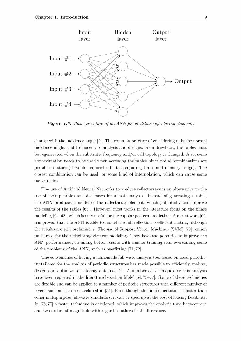
Chapter 1. Introduction 9
Input #1
Input #2
Input #3
Input #4
Output
Hiddenlayer
Inputlayer
Outputlayer
Figure 1.5: Basic structure of an ANN for modeling reflectarray elements.
change with the incidence angle [2]. The common practice of considering only the normal
incidence might lead to inaccurate analysis and designs. As a drawback, the tables must
be regenerated when the substrate, frequency and/or cell topology is changed. Also, some
approximation needs to be used when accessing the tables, since not all combinations are
possible to store (it would required infinite computing times and memory usage). The
closest combination can be used, or some kind of interpolation, which can cause some
inaccuracies.
The use of Artificial Neural Networks to analyze reflectarrays is an alternative to the
use of lookup tables and databases for a fast analysis. Instead of generating a table,
the ANN produces a model of the reflectarray element, which potentially can improve
the results of the tables [63]. However, most works in the literature focus on the phase
modeling [64–68], which is only useful for the copolar pattern prediction. A recent work [69]
has proved that the ANN is able to model the full reflection coefficient matrix, although
the results are still preliminary. The use of Support Vector Machines (SVM) [70] remain
uncharted for the reflectarray element modeling. They have the potential to improve the
ANN performances, obtaining better results with smaller training sets, overcoming some
of the problems of the ANN, such as overfitting [71,72].
The convenience of having a homemade full-wave analysis tool based on local periodic-
ity tailored for the analysis of periodic structures has made possible to efficiently analyze,
design and optimize reflectarray antennas [2]. A number of techniques for this analysis
have been reported in the literature based on MoM [54,73–77]. Some of these techniques
are flexible and can be applied to a number of periodic structures with different number of
layers, such as the one developed in [54]. Even though this implementation is faster than
other multipurpose full-wave simulators, it can be sped up at the cost of loosing flexibility.
In [76, 77] a faster technique is developed, which improves the analysis time between one
and two orders of magnitude with regard to others in the literature.

10 1.2. State of the art
1.2.3. Incident and radiated fields
For a proper analysis of reflectarray antennas, not only the elements have to be accu-
rately characterized by means of a full-wave technique; the feed and radiation patterns
computation also play a role in the correct characterization of the radiated far fields.
The feed pattern can be approximated by a far field ideal model, i.e. a cosq θ function or
a Gaussian beam [78,79]. These models have been demonstrated to be useful for modeling
the main beam of horn antennas and they are used to compute the incident field on the
reflectarray surface. They are widely used since they have several parameters that permit
to determine the characteristics that should be achieved by the actual feed. The calculation
of the impinging wave phase from the feed is based on the concept of the antenna phase
center and the distance from it to the center of the reflectarray element. Although the
phase center is different for the E and H planes of the feed, an intermediate value can
be taken for the analysis of the reflectarray. Thus, in many practical configurations, the
focal distance is defined in the design process so that the reflectarray is in the far field
zone of the feed and the ideal far field model is valid [2]. However, in some configurations,
the far field approximation is inappropriate because the reflectarray elements are placed
on the Fresnel zone of the primary feed, as for example, when the reflectarray is fed
by a high gain feed, or in the case of dual-reflector configuration using a reflectarray as
subreflector [80, 81]. In those cases, the real near field of the primary feed can be used to
improve the results [82]. Also, the aperture efficiency can be improved by tailoring the
design of the feed antenna [83]. In [84] a semi-analytical method is proposed to compute
the incident field on the entire plane that contains the reflectarray using a discrete plane-
wave expansion. It can be used for any arbitrary excitation and improves the results
of [82], but it is computationally more expensive.
Since the reflectarray is an aperture, its radiation patterns can be calculated using the
Equivalence Principles [2]. The most time consuming operation is the computation of the
spectrum functions, which are calculated as the Fourier transforms of the tangential field
on the aperture [85]. For regular grids, this operation can be efficiently performed using the
Fast Fourier Transform (FFT) [2], modeling each reflectarray element as a small aperture
instead of a punctual source, which is more accurate. However, for the aperiodic case the
element is considered a punctual isotropic source, since only the array factor is taken into
account [86,87]. When the reflectarray element is modeled as a small aperture, the field at
each cell is considered constant, which is convenient because it facilitates operating with
the equations. Little research has been carried out considering a continuous incident field
in an efficient fashion.
Finally, it is very common to compute the reflectarray far fields using the Second
Principle of Equivalence [2], which only considers the electric field on the reflectarray
surface. However, it has been demonstrated [43,88] that the First Principle is more suitable
for both the copolar and crosspolar patterns prediction. The First Principle of Equivalence
uses both the electric and magnetic fields on the reflectarray surface, and thus the number
of spectrum functions to evaluate is double with regard to the Second Principle. However,
all of them can be efficiently computed by means of the FFT algorithm, and the increased

Chapter 1. Introduction 11
computational effort is acceptable.
1.2.4. Reflectarray pattern synthesis
The antenna synthesis problem can be viewed as the inverse of the analysis problem. In
the analysis problem, given the antenna full structure, the radiated field is obtained. Con-
versely, in the antenna synthesis, given a set of field specifications, the antenna geometry
is sought so that it fulfills the specified requirements. Although in a very general case
any aspect of the antenna is suitable to be optimized in the synthesis process, such as
its structure, feed system, etc., and there are algorithms that are able to deal with this
generalized problem [89], it is more common to work with a simplified case, in which the
antenna structure and feed system are fixed and known beforehand.
The most common technique for the synthesis of shaped-beam reflectarrays is known
as Phase-Only Synthesis (POS). Since the phases of the direct reflection coefficients di-
rectly control the shape of the copolar pattern, the POS only works with these phases,
enormously simplifying the reflectarray analysis. Despite all the simplifications, this tech-
nique is able to provide accurate results and achieve very complex shaped-beams. The
main disadvantage is that it only works with the copolar patterns, and there is no control
over the crosspolar ones during the synthesis process.
In order to achieve the required specifications, a number of algorithms has been used
to synthesize the radiation patterns in the POS case, for instance, analytical [90,91], steep-
est descent [92], conjugate gradient [93], Intersection Approach (IA) [94, 95], Levenberg-
Marquardt Algorithm (LMA) [96,97], genetic algorithms [98] or particle swarm optimiza-
tion [21, 99], among others. However, the analytical approaches have limitations when
applied to complex shaped patterns, although they can be used to generate a starting
point for a more powerful synthesis algorithm [81]. The steepest descent has a very slow
convergence rate [100,101], which makes it impractical to synthesize arrays with a moder-
ate number of elements. Conjugate gradient methods can be adapted to solve non-linear
optimization problems and are faster than the steepest descent [100], but they tend to
be both less efficient and less robust than quasi-Newton methods [101]. The intersection
approach is very efficient when using only the FFT, but suffers from the problem of traps
(i.e. local minima), due to the non-convexity of the sets dealt with [89]. One manner
of dealing with the trap problem is working with the far field squared amplitude instead
of just the amplitude or complex field [89, 102]. However, this approach causes that one
of the projectors of the intersection approach cannot be implemented with the FFT (the
projector which recovers the reflected field on the reflectarray surface), and a minimization
algorithm based on optimization techniques has to be used, greatly reducing the efficiency
of the intersection approach algorithm (in [102], the Broyden-Fletcher-Goldfarb-Shanno
(BFGS) algorithm is used, although other algorithms are also suitable, such as the LMA).
The LMA, has high memory requirements, due to the fact that it needs to store a Jaco-
bian and Hessian approximation matrices, which can limit its usage when optimizing large
antennas. Also, some expensive operations, such as a big matrix multiplication, needs to
be performed, slowing the computations. This operation may be avoided by using a QR

12 1.2. State of the art
x
f(x)
(a)
x
f(x)
(b)
Figure 1.6: Local vs. global search with the same starting point. (a) Local search finds alocal minimum. (b) Global search finds global minimum after a more exhaustive and timeconsuming exploration.
factorization, at the expense of more memory usage [100]. All these algorithms are local
optimizers and depend strongly on the starting point to converge with success.
Genetic algorithms (GA) and particle swarm optimization (PSO) are global search
algorithms, which in contrast with the previous local search algorithms, do not depend
on the starting point. These algorithms are potentially able to find the global maximum
at the expense of taking many iterations. However, as the number of variables increase,
the search space size grows exponentially, making it harder for these algorithms to find
a suitable solution. Another aspect of evolutionary algorithms is that due to their non-
deterministic approach, two instances using the same parameters will yield different results,
in contrast with the deterministic approach of the local optimizers mentioned above. GA
and PSO have been demonstrated capable of synthesizing phased arrays, although at the
cost of several thousand iterations [103]. Each iteration involves several evaluations of
the cost function, one for each member of the population, thus making their computing
times very sensitive to the to the time cost of the cost function (also known as fitness in
evolutionary algorithm terms). Both algorithms seem to have similar performance with
small arrays, although PSO is easier to implement [103]. Recently, the PSO has been used
to synthesize several reflectarray radiation patterns [21,99]. In [21], a single-fed reflectarray
of 848 elements with asymmetric multiple beams was synthesized, taking more than 70 000
iterations to converge and 44 hours. In [99], a reflectarray of 900 elements was synthesized,
taking 5500 iterations to converge. Increasing the size of the antenna would dramatically
increase computing times to achieve convergence with these algorithms because of their
global search approach, unless a suitable starting point was used and the PSO was set up
to prioritize local search.
Other global search algorithms, less common in antenna synthesis than the two al-
gorithms mentioned above, are the differential evolution [104, 105], ant colony optimiza-
tion [106, 107], firefly algorithm [108], bacterial foraging optimization [109, 110], biogeog-
raphy based optimization [111] and the Taguchi method [112], among others.
Regarding memory usage, the LMA presents a disadvantage with regard to other syn-

Chapter 1. Introduction 13
thesis algorithms. The LMA needs to store a Jacobian matrix, which is generally bigger
than the Hessian matrix (or its approximation) used by Newton and quasi-Newton meth-
ods. Additionally, the LMA also needs to store the approximation of the Hessian. In
contrast, the conjugate gradient only needs to store a smaller matrix (same size as the
Hessian) and a few vectors, while the steepest descent only stores vectors. The intersec-
tion approach uses one to four small matrices with dimension the number of samples of
the radiation pattern. (When an optimization algorithm is introduced in the intersection
approach, the storage needs would be the same as the ones of the optimization algorithm
plus the needs of the intersection approach.) Evolutionary algorithms, such as GA or
PSO, store one solution per member of the population. In the phase-only synthesis case,
the solution is a vector or matrix with the number of elements equal to the number of
unknowns. Exact storage needs for the mentioned algorithms will vary according to their
implementations, although they have been roughly laid out for the main data structures.
The LMA trades more memory usage for a more robust algorithm for non-linear opti-
mization when compared with other gradient methods, and a less powerful framework
when compared with the intersection approach. The LMA is also simpler and easier to
implement than other quasi-Newton methods, and is faster than evolutionary algorithms
due to its local search nature.
As an example, a reflectarray of Nx×Ny elements (which correspond to the unknowns
of the problem) is considered, computing the radiation pattern only for one polarization
in a grid with Mu × Mv points. The evolutionary algorithms are considered to have
L members in their population. Note that, in general, Nx · Ny ≤ Mu · Mv. In this
case, the size of the Jacobian matrix is Nx · Ny · Mu · Mv, the size of the Hessian or
its approximation is N2x · N2
y and the size of a solution is Nx · Ny. Then, the memory
usage is O(Nx ·Ny ·Mu ·Mv +N2x ·N2
y ) for the LMA, corresponding to the Jacobian and
approximation of the Hessian; O(N2x · N2
y ) for quasi-Newton methods and the conjugate
gradient, corresponding to the Hessian or its approximation; O(Nx · Ny +Mu ·Mv) for
the intersection approach, corresponding to a solution and the computed far field; and
O(L ·Nx ·Ny + L ·Mu ·Mv) for the GA and PSO, corresponding to one solution and one
computed far field per member of the population. Auxiliary vectors and matrices might
be used depending on the implementation, but the main data structures shown above take
up most of the memory used by the algorithm.
As stated before, the POS technique has demonstrated to be very effective in the design
of reflectarrays that fulfill very stringent requirements, for instance [19,20]. However, since
it is a POS, it has no control over the crosspolar far fields during the synthesis process.
Some techniques for lowering the crosspolarization of reflectarrays have been described
which rely on positioning the elements in certain configurations [113] or by adjusting the
elements dimensions forcing a null in the amplitude and a change of sign in the phase of the
crosspolar reflection coefficients [114, 115]. However, these techniques present limitations
and are not flexible, since they only try to reduce the contribution of the cross-coefficients
after the synthesis is done, instead of synthesizing the crosspolar pattern to a desired
value. This latter approach was followed in [116–118], where the Intersection Approach is

14 1.3. Thesis goals
used along with the Broyden-Fletcher-Goldfarb-Shanno (BFGS) optimization algorithm
as backward projector. However, only single-polarized reflectarrays were considered with
very few elements (225 in total) since the algorithm was slow. More recently, some works
have appeared that deal with dual-polarized reflectarrays with crosspolar constraints. For
instance, in [17], a faceted dual-polarized reflectarray with crosspolar suppression is pre-
sented, where after a POS pattern is obtained, the crosspolar component is suppressed
and the currents on the surface of the reflectarray are obtained. From there, the matrix
of reflection coefficients are computed, which fully characterize the reflectarray element.
Finally, in [119–121] a general optimization technique for printed reflectarrays is presented
and used, which employs a gradient minimax algorithm for the direct optimization of the
reflectarray geometry. It allows to synthesize both copolar and crosspolar components
using several degrees of freedom. Nevertheless, it uses a look-up table of scattering pa-
rameters to speed up computations during the optimization process, which needs to be
generated for each substrate and unit cell. However, as the number of optimizing variables
is increased, the times required to generate the table rapidly increase as well. Furthermore,
to create the table some variables which are not needed during the optimization process
(i.e. they are not optimized) are considered, such as the pair of incident angles, since for
a given reflectarray geometry, varying the incident angle can modify the reflection coeffi-
cients. Also, because interpolation is used to calculate the scattering parameters from the
look-up table, precision is lost, which is essential for the crosspolar optimization, since its
behavior is highly non-linear and its absolute values are very low with regard to those of
the copolar component.
1.3. Thesis goals
This thesis is devoted to the analysis and synthesis of reflectarray antennas in single-
offset configurations. The goals are divided in three blocks: the development of efficient
techniques for reflectarray analysis, the improvement of the synthesis of the copolar far
field component, and the development of efficient algorithms for the reflectarray crosspolar
optimization.
The reflectarray analysis can be divided in a number of steps, including the analysis
of the feed, the reflectarray element and the computation of radiation patterns. Each
one of these subanalyses can be independently improved to speed up computations and
obtain higher numerical accuracy. With regard to the computation of radiation patterns,
efficient and accurate techniques are available for periodic reflectarrays. The efficiency
lies in the use of the FFT algorithm for the computation of the spectrum functions, and
the accuracy in the consideration of the reflectarray element as a small aperture instead
of a punctual source. However, for aperiodic reflectarrays there is no such technique that
includes both considerations. If the NUFFT were used, the reflectarray elements can be
only be analyzed as punctual sources. Conversely, if they were analyzed as small apertures,
a direct evaluation of the spectrum functions would need to be implemented, since the
NUFFT cannot be directly applied. Thus, the first goal of this thesis is to develop an

Chapter 1. Introduction 15
efficient and accurate technique for the analysis of aperiodic reflectarrays which presents
the same capabilities as the analysis of periodic reflectarrays.
The reflectarray analysis usually considers the incident field from the feed to be con-
stant at each reflectarray element. This is convenient because it facilitates the analytical
operations with the equations. A generalization of the analysis considering a variable
incident field at each cell will be proposed to improve the accuracy while still keeping
the analysis efficiency. This generalization will be developed for both cases, periodic and
aperiodic reflectarrays using the FFT and NUFFT algorithms, respectively.
The characterization of the reflectarray far fields can be improved by using the First
Principle of Equivalence instead of the Second Principle, since it also takes into account the
magnetic field on the reflectarray aperture. In addition, reflectarray antennas usually have
a dielectric frame backed by a ground plane at the edges. This frame is a continuation of the
reflectarray breadboard without metallizations and needs to be conveniently characterized
to correctly predict the far fields.
Array near field models usually consider each element as punctual isotropic sources.
It is proposed to improve those models by modeling the reflectarray element as a small
aperture, as in the case of far field analysis. The aim of improving this model is its use
within an optimization algorithm in order to be able to develop techniques for the near
field synthesis of reflectarray antennas.
The second and third blocks are closely related since they both comprise the develop-
ment of efficient techniques for the synthesis of reflectarray antennas. The second block
is aimed to the improvement of the copolar synthesis, by including the First Principle of
Equivalence in the phase-only synthesis as well as the characterization of the dielectric
frame. In addition, an improved POS technique will be developed which will allow the
future crosspolar optimization developed in the third block, as well as its extension to near
field phase-only synthesis with the model previously improved.
The third block of the thesis is focused on the crosspolar optimization of reflectarray
antennas. Typically, reflectarray synthesis techniques are based on phase-only techniques,
which can only impose copolar specifications during the synthesis process and there is no
control over the crosspolar component. Some techniques to improve the crosspolar far field
have been devised for the case of reflectarray antennas, although they are limited. Only
recently some works have addressed the crosspolar optimization of reflectarrays, relying
on look-up tables for the reflection coefficient matrices. Thus, another goal of the thesis
is the development of efficient algorithms for the crosspolar optimization of reflectarray
antennas, that add new contributions to this recent opened research line.
1.4. Thesis outline
The present thesis has been organized in six chapters, including this one for the introduc-
tion and the last one for summarizing the main ideas and novel contributions of the thesis.
The remain chapters include the analysis and synthesis techniques developed as well as
examples to demonstrate and validate the presented original contributions.

16 1.4. Thesis outline
Chapter 2 is devoted to the analysis of a single offset reflectarray antenna and the
computation of its radiated fields. It starts with the equivalent parabolic reflector geometry
and from the parabolic reflector parameters, the reflectarray is geometrically characterized.
Then, the analysis to obtain the tangential field on the surface of the reflectarray from
the incident field of the feed is described. The feed is usually a horn antenna, which is
modeled as a mathematical function in order to simplify the analysis. The tangential field
is obtained analyzing the reflectarray with a full-wave Method of Moments (MoM) based
on local periodicity in order to account for substrate losses and other effects introduced
by the reflectarray element. The reflected tangential magnetic field is derived from the
reflected electric field from the plane wave relation at each reflectarray element. The
magnetic field is necessary in order to compute the far fields using the First Principle
of Equivalence, which characterizes the radiated fields better than the Second Principle.
Then, an efficient technique to compute the far fields from the tangential field is described,
which is based on the Fast Fourier Transform (FFT) algorithm. This technique is only
suitable for periodic reflectarrays and is later extended to aperiodic reflectarrays employing
the Non-Uniform FFT (NUFFT). This analysis technique is later generalized assuming a
continuous variable incident field across the reflectarray surface. Numerical examples are
provided to show the capabilities of the new developed techniques. Finally, a new model
for the computation of the reflectarray near field is presented and validated.
Chapter 3 describes the Intersection Approach (IA) for Phase-Only Synthesis (POS),
a widely used algorithm to obtain shaped-beam reflectarrays. Its formulation is presented
for the Second Principle of Equivalence and is then extended to the First Principle. The
success of this algorithm lies in its computational efficiency due to its use of the FFT, which
is its most time consuming operation, and the ability to handle very large reflectarrays.
Some techniques for the convergence improvement and design control are presented, along
with an example of a reflectarray with an isoflux pattern for global Earth coverage. Since
the IA-POS only deals with copolar requirements, the IA formulation is extended in an
efficient fashion to include crosspolar requirements during the synthesis process. The
resulting algorithm (IA-XP) is still computationally efficient since it is still based on the
use of the FFT. Some examples are provided to validate the developed algorithm.
Chapter 4 is dedicated to the optimization of the Levenberg-Marquardt Algorithm
(LMA) for reflectarray POS, since the formulation of the IA in Chapter 3 presents some
inconveniences: it is difficult to obtain a reflectarray layout with the IA-XP and neither
the IA-POS nor the IA-XP can be used for near field synthesis. The chosen algorithm is
the LMA, which is extensively detailed and optimized in this chapter for POS. The two
formulations of the IA presented in Chapter 3 were only suitable for far field synthesis.
However, the LMA developed in this chapter is also used for near field optimization, only
changing the analysis tool. The reflectarray quiet zone is optimized with the goal of
obtaining reflectarrays for their use as probes for Compact Antenna Test Ranges (CATR).
Chapter 5 addresses the crosspolar optimization in reflectarrays by performing a direct
optimization of the antenna geometry. For this optimization, a full-wave analysis based
on local periodicity of the reflectarray element is used directly in the optimization loop,

Chapter 1. Introduction 17
employing the Method of Moments (MoM) in spectral domain. The techniques developed
in this chapter take advantage of the work done in previous chapters. First, an extension
of the LMA previously developed (LMA-POS) is realized in order to carry out cross-
polar optimization of reflectarrays (LMA-XP). Although the LMA-POS was thoroughly
improved, now that MoM is used in the optimization process, some further improvements
are introduced to minimize the impact of MoM, by reducing the number of calls needed
to the MoM routine. The LMA-XP effectively reduces the crosspolar component of the
far field while preserving the copolar shape, although it presents some convergence issues
for large reflectarrays. Hence, a new algorithm is developed in order to improve the con-
vergence of the LMA-XP. This new algorithm is based on the IA framework and works
with the squared field amplitude. The backward projector is modified to use the LMA and
the resulting algorithm is known as IA-LMA-XP. It can handle thousands of optimizing
variables and reduce the crosspolar component of very large reflectarrays, as demonstrated
in the provided test cases.
Finally, Chapter 6 contains the final conclusions of the work presented in the thesis, as
well as a summary of the original contributions, a number of future lines of research opened
during the development of this work and a list of the published papers in international
journals and conferences.


CHAPTER 2
Efficient analysis of printed
reflectarrays
2.1. Introduction
A printed reflectarray consists of a planar array of printed radiating elements, such as
patches with stubs, rectangular patches, parallel dipoles, rings, crosses, etc., in a single
or multiple stacked layers backed by a ground plane and illuminated by a feed. Although
the list of reflectarray element topologies is wide, the operating principle is always the
same. The reflectarray is illuminated by a primary feed, typically a horn antenna (al-
though other types are possible). The incident field from the feed is reflected back by the
radiating elements introducing a phase-shift in the field. This phase-shift can be modified
by adjusting one or several parameters of the reflectarray element geometry. Hence, the
phase distribution of the tangential field can be controlled in order to collimate or shape
the beam.
The analysis of the reflectarray is divided in several steps throughout this chapter.
First, the geometry of the antenna is analyzed. In this work, the single-offset configuration
is considered. This configuration is based on an equivalent parabolic reflector setup defined
by the equivalent or projected aperture, the focal distance and the clearance. From these
parameters the reflectarray parameters can be derived.
Then, the incident field on the reflectarray surface is obtained. It is usually done by
modeling the feed with a far field ideal model, which only takes into account the main
beam. However, side lobes of the real feed usually fall at angles outside the surface of
the reflectarray, so this model provides a good enough approximation for the feed. The
computation of the impinging wave phase from the feed is based on the concept of the
antenna phase center and the distance from it to the center of the reflectarray element.
In order to obtain the reflected or tangential field, it is necessary to know how the
reflectarray elements affect the incident field from the feed. Ideally, only a phase shift
would be produced, although in reality the amplitude is slightly changed and crosspolar
components are added to the field. The reflectarray element is analyzed using the Method
19

20 2.2. Geometry of the equivalent parabolic reflector
of Moments (MoM) in spectral domain and the Floquet theorem assuming local periodicity.
This means that each element is analyzed by embedding the element in an infinite array
comprised of the same element, taking into account mutual coupling between elements.
Due to this fact, it is important that reflectarray designs present phase distributions that
are smooth, since for similar phases, the dimensions of the elements are also similar, thus
preserving the local periodicity assumption. With this analysis, the matrix of reflection
coefficients is obtained. This matrix relates the incident field with the reflected field on
the surface of the reflectarray and accounts for the phase shift, losses due to the substrate
and crosspolarization introduced by the element.
Once the reflected field has been obtained, it is used to compute the radiated far fields.
Since the reflectarray is an aperture antenna, the Equivalence Principles can be employed
in the calculation of the far fields. Depending on the available knowledge on the electric
and magnetic fields, the First, Second or Third Equivalence Principles may be used. In
practice, it is common to only work with the electric field, so the Second Principle of
Equivalence is used. In any case, all of them require the computation of the spectrum
functions, which are obtained as the Fourier transform of the tangential field, and is the
most time consuming operation in the calculation of the far field. For this reason, the
Fast Fourier Transform (FFT) can be used in order to efficiently compute the spectrum
functions for a periodic reflectarray. However, when the grid is aperiodic, the FFT can
no longer be used and, in order to preserve the efficiency, the non-uniform FFT (NUFFT)
must be employed.
Finally, from the tangential field the near field radiated by the reflectarray can also be
obtained. A near field model is developed and validated, in which each reflectarray element
is considered a radiation unit and is modeled as a small aperture. The total near field is
obtained as far field contributions from all the reflectarray elements. Then, this model is
validated through simulations with the commercial software GRASP and measurements
from a reflectarray antenna.
2.2. Geometry of the equivalent parabolic reflector
This section is devoted to the geometrical definition of the reflectarray antenna under
study. The most common configuration in the literature is the single-offset reflectarray [2]
(from which the centered configuration is a particular case), although there exist others
having the reflectarray as subreflector of a main parabolic reflector [80, 122] or a dual
reflectarray setup [115,123]. Due to its simplicity, the single-offset configuration has been
selected and a sketch is shown in Figure 2.1. This configuration is based on an equivalent
parabolic reflector setup defined by the equivalent or projected aperture D, the focal
distance F and the clearance C. (The centered configuration would be defined by C =
−D/2.) From these parameters and the equation of an elliptic paraboloid, the reflectarray
parameters can be derived.
The equation of the elliptic paraboloid surface (from which the parabolic reflector is a
section of its surface) is
x2 + y2 = 4Fz, (2.1)

Chapter 2. Efficient analysis of printed reflectarrays 21
Focus
Reflectarray
Equivalent parabolic reflector
y
x
z
yr
xr
zr
zaθ0
F
C
D
P1
P2
Figure 2.1: Sketch of a single-offset reflectarray and its equivalent parabolic reflectorsystem.
where F is the focal distance as shown in Figure 2.1. The reflectarray is placed in the
chordal plane of the parabolic reflector. In the following sections, important reflectarray
parameters will be derived starting from eq. (2.1).
2.2.1. Focus in the reflectarray coordinate system
When analyzing the reflectarray, it is common to do it in its own coordinate system
(xr, yr, zr), see Figure 2.1. Hence, we have to express the reflectarray parameters in
that coordinate system, in particular the focus coordinates, where the feed will be placed.
The focal point coordinates in the Global Coordinate System (GCS) are (xf , yf , zf )GCS =
(0, 0, F ). In order to obtain the coordinates in the Reflectarray Coordinate System (RCS),
we need to obtain the change of basis matrix. This can be done by expressing the vectors
xr, yr, zr in the (x, y, z) basis. In the XZ plane with y = 0, (2.1) is reduced to the
parabola equation
x2 = 4Fz. (2.2)
The reflectarray is resting in the parabolic reflector at the points P1 = (x1, z1) and P2 =
(x2, z2). Knowing that x1 = C, x2 = C +D and using (2.2) both points are obtained as
P1 =
(C,
C2
4F
), (2.3a)
P2 =
(C +D,
(C +D)2
4F
). (2.3b)

22 2.2. Geometry of the equivalent parabolic reflector
Once P1 and P2 are obtained, vector xr can be easily calculated as
~xr = (x2 − x1) x+ 0 y + (z2 − z1) z = (C +D − C) x+ 0 y +
((C +D)2
4F− C2
4F
)z
= D x+ 0 y +1
4F
(C2 + 2CD +D2 − C2
)z = D x+ 0 y +
D(2C +D)
4Fz,
(2.4)
‖~xr‖ =
√D2 +
D2(2C +D)2
16F 2=
D
4F
√16F 2 + (2C +D)2, (2.5)
xr =~xr‖~xr‖
. (2.6)
Since yr = y, only zr is left, and can be easily calculated as the cross product of xr and
yr, zr = xr × yr. Operating:
zr = xr × yr =
∣∣∣∣∣∣∣∣∣x y z
D‖~xr‖ 0 D(2C+D)
4F‖~xr‖
0 1 0
∣∣∣∣∣∣∣∣∣ = x
(0− D(2C +D)
4F‖~xr‖
)− y (0− 0) + z
(D
‖~xr‖
)
= −D(2C +D)
4F‖~xr‖x+
D
‖~xr‖z. (2.7)
Once the vectors xr, yr, zr are obtained, the change of basis matrix from GCS to RCS
is calculated simply by putting these vector as rows of said matrix. In order to obtain
the focus coordinates in the RCS, the vector [(0, 0, F )− (center of the RA)] needs to be
transformed. The center of the reflectarray is(x1 + x2
2, 0,
z1 + z22
)=
(2C +D
2, 0,
C2 + (C +D)2
8F
). (2.8)
Then, the vector to be transformed is
~v = (0, 0, F )−(x1 + x2
2, 0,
z1 + z22
)=
(−2C +D
2, 0,
8F 2 − C2 − (C +D)2
8F
). (2.9)
Finally, the coordinates of the focus (feed) in the reflectarray coordinate system will bexf
yf
zf
(RCS)
=
D
‖~xr‖ 0 D(2C+D)4F‖~xr‖
0 1 0
−D(2C+D)4F‖~xr‖ 0 D
‖~xr‖
−2C+D2
0
8F 2−C2−(C+D)2
8F
(GCS)
. (2.10)
2.2.2. Number of reflectarray elements
Given the reflectarray periodicity (a, b), being a the periodicity in the xr axis and b in the
yr axis, the maximum number of elements in each axis can be calculated. The reflectarray
length along xr is given by ‖~xr‖, defined in (2.5), so the number of elements in that axis

Chapter 2. Efficient analysis of printed reflectarrays 23
will be
Nx =
[‖~xr‖a
], (2.11)
where [] denotes the nearest integer function. As the paraboloid has symmetry of revo-
lution, it will be extended in the yr axis y = ±D/2, (see Figure 2.1), hence the number of
elements in that direction will be
Ny =
[D
b
]. (2.12)
2.2.3. Radiation angle
Another parameter of interest is the radiation angle, which in general is (θ0, ϕ0). From
the GCS point of view, a beam-focused reflectarray will collimate the rays from the feed
in the z axis and thus ϕ0 = 0. The angle formed by z (or equivalently, za) and zr will be
the pointing angle (see Figure 2.1), which can be easily obtained as the dot product of the
two angles,
z · zr = ‖z‖ ‖zr‖ cos θ0 = cos θ0 ⇒ θ0 = arccos (z · zr) . (2.13)
Vector zr was previously obtained in (2.7), and taking into account that the norm of the
unitary vectors is one, the dot product will be
z · zr = (0, 0, 1)
−D(2C+D)
4F‖~xr‖
0
D‖~xr‖
=D
‖~xr‖⇒ θ0 = arccos
(D
‖~xr‖
), (2.14)
where ‖~xr‖ has been obtained in (2.5).
2.2.4. Targonsky condition
When designing directive reflectarrays for far field applications, the pointing direction of
the main beam changes with frequency. This effect is known as beam squint and it also
exists in offset parabolic reflectors. It can be minimized by imposing [124]
θi = θ0, (2.15)
where θi is the pointing angle of the feed over the reflectarray surface and θ0 the radiation
angle (see Figure 2.2). When imposing this condition, the point xi where the feed is
pointing at on the reflectarray surface will change. Usually, xi is chosen to minimize
the spillover [125] by imposing an almost constant illumination taper at the reflectarray
contour edge. Thus, if the Targonski condition is met the spillover will not be minimized
for a given feed.
In order to calculate the new xi point, Figure 2.2 will be used as reference. The feed
coordinates are (xf , 0, zf ) (with yf = 0, since the feed is considered to be in the XZ
plane) and the incident and radiation angles fulfill θi = θ0. The distance of the focus with
regard to xi will be
xoff = zf tan θ0 > 0, (2.16)

24 2.3. Analysis of reflectarrays based on local periodicity
xr
zrFeed at (xf , yf , zf )RCS
xi
xoff
zf
xf
θiθ0
Figure 2.2: Illustration of the Targonski condition to minimize the beam squint.
and it is always a positive value. Then, taking into account the position of the feed, it
follows
xi = xf + xoff. (2.17)
According to Figure 2.1, xf will be always negative in the RCS, and thus xi can be positive
or negative depending on the values of xf and xoff.
2.3. Analysis of reflectarrays based on local periodicity
Once the geometry of the antenna has been characterized and the reflectarray parameters
derived from the parabolic reflector equivalent model, the tangential field on the surface
of the reflectarray needs to be computed. This will be done first by analyzing the field
radiated by the feed antenna, which will be modeled with an ideal far field model, suitable
for directive antennas such as horns. The analysis will consider a dual linear polarized
reflectarray whose working polarization will depend on the polarization of the feed, which
can be X- or Y-polarized, as seen in Figure 2.3.
Then, the reflectarray will be analyzed using a full-wave analysis based on local peri-
odicity and the Floquet theorem in order to obtain the reflection coefficient matrix that
relates the incident with the reflected field. This full-wave analysis takes into account
mutual coupling between elements, the field reflected by the substrate and ground plane,
the field reradiated by the metallizations, and substrate losses.
With this method of analysis, three sources of cross-polarization are taken into account:
the crosspolar component due to the incident field from the feed (if a real model were used),
the geometry through the projection of the incident field onto the reflectarray surface and
the crosspolarization introduced by the reflectarray element.

Chapter 2. Efficient analysis of printed reflectarrays 25
yr
xr
zr
~rfzf
−yf
xf
Figure 2.3: Scheme of a general printed reflectarray.
2.3.1. Feed model
Before addressing the actual analysis of the reflectarray antenna, the incident field on its
surface needs to be calculated. It depends on the position and radiation pattern of the
feed as shown in Figure 2.3. Usually, a horn antenna is used as feed and its radiation
pattern can be modeled as a function. The model used is the one proposed in [78], where
the following expressions for the horn far field are provided for an X- and Y-polarized feed
horn expressed in the Feed Coordinate System (FCS) (xf , yf , zf ),
~EX = jA0k02πr
e−jk0r[CX (θ) cosϕ θ − CY (θ) sinϕ ϕ
], (2.18a)
~EY = jA0k02πr
e−jk0r[CX (θ) sinϕ θ + CY (θ) cosϕ ϕ
], (2.18b)
where k0 is the wavenumber in vacuum and A0 is a constant that depends on the radiated
power. According to Figure 2.3, when the feed horn is X-polarized, the electric field is
aligned with the xf axis. Conversely, for a Y-polarized feed horn, the electric field is
aligned with the yf axis. CX(θ) and CY (θ) are functions that give the feed horn pattern
in the XZ and YZ planes of the FCS respectively,
CX(θ) = cosqx θ, (2.19a)
CY (θ) = cosqy θ. (2.19b)
Both axial symmetric and non-symmetric radiation patterns can be modeled with (2.18),
considering q = qx = qy or qx 6= qy in (2.19), respectively. The q factor gives the beamwidth
in the main planes of the feed radiation patterns and thus the directivity of the feed (see
Figure 2.4). This ideal model only characterizes the main lobe of the radiation pattern of
the feed, as seen in Figure 2.4. Thus, it is only suitable for directive antennas, such us
horns, where the side lobes are low, or when the projection of the side lobes lay outside

26 2.3. Analysis of reflectarrays based on local periodicity
−60 −50 −40 −30 −20 −10 0 10 20 30 40 50 600
0.1
0.2
0.3
0.4
0.5
0.6
0.7
0.8
0.9
1
θ ()
cosq
θq = 10q = 15q = 20q = 25q = 30q = 35
(a)
−60 −50 −40 −30 −20 −10 0 10 20 30 40 50 60−50
−45
−40
−35
−30
−25
−20
−15
−10
−5
0
θ ()
cosq
θ(dB)
q = 10q = 15q = 20q = 25q = 30q = 35
(b)
Figure 2.4: Radiation pattern given by a cosq θ function for different q values. (a) Nat-ural units. (b) Decibels.
the surface of the reflectarray, i.e., its surface is only illuminated by the main lobe. In
those cases, this model provides good enough results to use it in the analysis, design and
synthesis of reflectarrays [2].
Since the function cosq θ is proportional to the amplitude of the electric field∣∣∣ ~E∣∣∣ ∝ cosq θ, (2.20)
the power (gain) will be proportional to the squared function∣∣∣ ~E∣∣∣2 ∝ cos2q θ, (2.21)
so the normalized gain of the horn will be equal to
G (θ) = 10 log(cos2q θ
)= 20 q log (cos θ) , (2.22)
for the main lobe of the radiation pattern. Isolating the variable yields
q =G (θ)
20 log (cos θ). (2.23)
This way, evaluating the normalized gain for several θ angles belonging to the main beam
and applying (2.23), a table of q values is obtained, which should be similar for θ angles
where the main beam can be approximated by a cosine function. For the two main planes,
two different values of q are be obtained, as shown in (2.19). Sometimes, an averaged q
value is used,
q =qx + qy
2, (2.24)
if qx and qy are similar [2,81]. This factor also changes with frequency since the directivity
of the horn antenna also does, so if the analysis is made at several frequencies, the feed
model needs to be obtained at each frequency [81].

Chapter 2. Efficient analysis of printed reflectarrays 27
The power radiated by the feed model is needed in order to compute the gain of the
reflectarray antenna. Since this feed model is ideal both the ohmic losses and the back
radiation are considered to be zero, and the sidelobes are neglected. However, for feed
horns the losses are typically in the order of 0.05 dB and thus negligible, the back radiation
is also very small and the level of the sidelobes will not significantly affect the final result.
As a result, the total power radiated by the feed can be computed as
Pfeed =
π/2∫θ=0
2π∫ϕ=0
∣∣∣ ~EX/Y (θ, ϕ)∣∣∣2
2η0r2 sin θ dθ dϕ, (2.25)
where ~EX/Y (θ, ϕ) is the field radiated by the ideal horn given by (2.18), and where X
and Y indicates the considered polarization from the feed. The squared amplitudes for
both polarizations are ∣∣∣ ~EX∣∣∣2 = ∣∣∣ ~EY
∣∣∣2 = A20
k20 cos2q θ
4π2 r2, (2.26)
where an axial symmetric pattern for the feed is considered. Substituting (2.26) in (2.25)
it follows
Pfeed = A20
π
η0 λ20 (2q + 1). (2.27)
The field radiated by the feed given by (2.18) is expressed in spherical coordinates in
the FCS (see Figure 2.3). However, the incident field should be expressed in Cartesian
coordinates of the RCS (xr, yr, zr). Thus, the field is first transformed to the Cartesian
coordinates of the FCS applying the following transformationE
X/Yx
EX/Yy
EX/Yz
(FCS)
=
sin θ cosϕ cos θ cosϕ − sinϕ
sin θ sinϕ cos θ sinϕ cosϕ
cos θ − sin θ 0
0
EX/Yθ
EX/Yϕ
(FCS)
. (2.28)
Note that this transformation is carried out for each element of the reflectarray, since the
incident angle (θ, ϕ) from the feed changes with the position of the element. Then, the
Cartesian components are transformed from FCS to RCS using [126]E
X/Yx
EX/Yy
EX/Yz
(RCS)
= A ·
E
X/Yx
EX/Yy
EX/Yz
(FCS)
=
a11 a12 a13
a21 a22 a23
a31 a32 a33
E
X/Yx
EX/Yy
EX/Yz
(FCS)
, (2.29)
where the columns of the A matrix are the director cosines of the FCS expressed in the
RCS. Thus, A defines the transformation of the field components from FCS to RCS and
is the same for all the reflectarray elements. The feed is placed at (xf , yf , zf ) and it
is oriented in such a way that points to a certain position in the reflectarray surface,

28 2.3. Analysis of reflectarrays based on local periodicity
(xi, yi, 0). Then, the zf axis is defined as
~zf = (xi − xf , yi − yf , −zf ) =⇒ zf =~zf‖~zf‖
. (2.30)
In general, the feed will be placed in a position not contained in the symmetry planes
of the reflectarray, and thus it will not be possible for the xf and yf feed axis to be
orthogonal to the yr and xr reflectarray axis at the same time, which is desirable to use
dual orthogonal polarization. In this general case, only one linear polarization will be
used.
X polarization, which must comply ~xf · yr = 0. Apart from this condition, it also
has to fulfill that ~xf must be orthogonal to zf , i.e. ~xf · zf = 0, so it immediately
follows that ~xf is orthogonal to yr and zf , or that
xf = yr × zf . (2.31)
From here, yf can be calculated as the cross product of xf and zf as
yf = zf × xf . (2.32)
The case for Y polarization is very similar. Now, it must comply ~yf · xr = 0, and
that the ~yf vector is orthogonal to zf , i.e. ~yf · zf = 0 , so, similarly to the previous
case, it follows
yf = zf × xr. (2.33)
Now, xf is obtained as
xf = yf × zf . (2.34)
Once the vectors (xf , yf , zf ) are obtained, they can be related to matrix A in (2.29).
Indeed, the columns of matrix A are the vectors (xf , yf , zf ),
xf = (a11, a21, a31), (2.35a)
yf = (a12, a22, a32), (2.35b)
zf = (a13, a23, a33). (2.35c)
For the case in which the feed is contained in the symmetry planes of the reflectarray,
such as in the case shown in Figure 2.1, the two conditions developed above are equivalent,
since the fulfillment of one of them implies the fulfillment of the other.
2.3.2. Tangential field on the surface of the reflectarray
2.3.2.1. Electric field
In the previous section, an ideal feed model was analyzed that provides the incident electric
field on the surface of the reflectarray, which can be written for both linear polarizations

Chapter 2. Efficient analysis of printed reflectarrays 29
as
~EX/Yinc (x, y) = E
X/Yinc,x (x, y) x+ E
X/Yinc,y (x, y) y, (2.36)
where the superscripts designate the polarization of the feed according to the FCS and the
subscripts the field component with regard to the RCS (e.g. EYx would be the x component
of the projected field over the reflectarray surface when the feed radiates in Y polarization).
Similarly, the reflected tangential electric field on the surface of the reflectarray can be
written as follows,
~EX/Yref (x, y) = E
X/Yref,x (x, y) x+ E
X/Yref,y (x, y) y. (2.37)
The relation between the incident and reflected tangential electric fields at each element
(m, n) of the reflectarray is given by a matrix of reflection coefficients that characterizes
that element,
~EX/Yref (xm, yn) = Rmn · ~EX/Y
inc (xm, yn), (2.38)
where (xm, yn) are the coordinates of the (m, n)th element and
Rmn =
ρmnxx ρmn
xy
ρmnyx ρmn
yy
. (2.39)
The components of Rmn are complex and fully characterize the behavior of the element.
The components ρxx and ρyy are known as direct coefficients while ρxy and ρyx are the
cross coefficients. The direct coefficients mostly affect the copolar radiation pattern for
each corresponding polarization (ρxx for X polarization and ρyy for Y polarization), while
both direct and cross coefficients are important in the computation of the crosspolar far
field. This latter fact can be easily seen by developing (2.38),
EX/Yref, x = ρxxE
X/Yinc, x + ρxy E
X/Yinc, y, (2.40a)
EX/Yref, y = ρyxE
X/Yinc, x + ρyy E
X/Yinc, y. (2.40b)
Assuming X polarization, the copolar reflected field is given by (2.40a) while the crosspolar
one is given by (2.40b). Regarding (2.40a), the following inequalities always occur,
|ρxx| |ρxy|∣∣∣EXinc, x
∣∣∣ ∣∣∣EXinc, y
∣∣∣ =⇒
∣∣ρxxEXinc, x
∣∣ ∣∣ρxy EXinc, y
∣∣ . (2.41)
According to this, the copolar reflected field can be approximated by
EXref, x ≈ ρxxE
Xinc, x. (2.42)
On the other hand, for the case of the crosspolar reflected field, it holds that
|ρyx| |ρyy| and∣∣EX
inc, x
∣∣ ∣∣EXinc, y
∣∣ , (2.43)

30 2.3. Analysis of reflectarrays based on local periodicity
+Einc,x
Einc,y
~Einc
ρxxEinc,x
ρyxEinc,x
ρxyEinc,y
ρyyEinc,y
Eref,x
Eref,y
~Eref
Figure 2.5: Decomposition of the incident field from a feed with no crosspolarization. Itshows the contributions to the crosspolarization from the field projection onto the reflect-array surface and the crosspolarization introduced by the reflectarray element.
so no term can be neglected in the sum. However, for the total reflected field, it follows
∣∣EXref, x
∣∣ ∣∣EXref, y
∣∣ , (2.44)
and since for the copolar radiation pattern the copolar reflected field is dominant, only
(2.42) is needed to correctly predict the copolar pattern with minimum error.
The two addends of the crosspolar reflected field have different sources. While ρyxEXinc,x
is produced by the crosspolarization introduced by the element due to ρyx, ρyy EXinc,y is
produced by the projection of the incident field from the feed onto the reflectarray surface.
They are graphically shown in Figure 2.5 and the effect is that the desired field component
remains almost the same while the crosspolarization considerably increases its value. If a
real feed is considered, its crosspolar contribution would add to both addends.
A similar discussion can be carried out for the Y polarization, where the following
inequalities in (2.40b) will be fulfilled,
|ρyy| |ρyx|∣∣∣EYinc, y
∣∣∣ ∣∣∣EYinc, x
∣∣∣ =⇒
∣∣ρyy EYinc, y
∣∣ ∣∣ρyxEYinc, x
∣∣ . (2.45)
As in the previous case, the copolar reflected field can be approximated by just one term
of the sum,
EYref, y ≈ ρyy E
Yinc, y. (2.46)
However, none of the terms of the crosspolar reflected field can be neglected since it holds

Chapter 2. Efficient analysis of printed reflectarrays 31
that
|ρxy| |ρxx| and∣∣EY
inc, y
∣∣ ∣∣EYinc, x
∣∣ . (2.47)
And as it happened for the X polarization, now the copolar far field can be correctly
predicted by (2.46).
Also, as in the previous case, the crosspolar reflected field for Y polarization has
two sources: the crosspolarization of the element, which produces one addend (ρxy EYinc,y,
through ρxy); and the reflectarray geometry through the projection of the incident field
onto the reflectarray surface, producing the other addend (ρxxEYinc,x, through E
Yinc,x). The
crosspolarization of a real feed would contribute to both addends of the crosspolar reflected
field.
The approximations in the reflected field given by (2.42) and (2.46) are used in phase-
only synthesis schemes, since it allows an important simplification of the Rmn matrix.
Indeed, in this case the reflectarray element is treated as an ideal phase shifter where there
are no losses and no crosspolarization introduced by the element. These two conditions
are expressed by
|ρxx| = |ρyy| = 1 (no losses) (2.48a)
|ρxy| = |ρyx| = 0 (no element crosspolarization), (2.48b)
and the Rmn matrix in (2.39) is simplified to
Rmn =
ejφmnxx 0
0 ejφmnyy
, (2.49)
where φ is the phase of the corresponding reflection coefficient. Now, the only two com-
ponents of the reflection coefficients matrix are the phases of the direct coefficients. Since
the incident field is fixed once the feed and its position are chosen, only the phases of ρxx
and ρyy will conform the copolar radiation pattern as desired, for X and Y polarizations,
respectively. This approximation has been widely used in the design of reflectarray anten-
nas [2], although it does not allow a direct control of the crosspolar far field in the synthesis
process, since the important contribution of ρxy and ρyx is not taken into account. This
causes that the crosspolar pattern cannot be accurately predicted with the simplification
of (2.49), as explained before with regard to the crosspolar reflected field, for which both
contributions are similarly important.
In order to be able to predict the crosspolar component of the radiation pattern, the
full Rmn matrix needs to be computed. Although there are more factors that affect the
crosspolar far field, it is important to correctly characterize the crosspolarization intro-
duced by the reflectarray element.

32 2.3. Analysis of reflectarrays based on local periodicity
2.3.2.2. Magnetic field
On the other hand, the tangential reflected magnetic field is computed at each reflectarray
element assuming a locally incident plane wave coming from the feed, using the following
expression [127]:
~HX/Yref (xm, yn) =
~kref × ~EX/Yref (xm, yn)
ωµ0, (2.50)
with ω = 2πf0 and ~kref~kref = kxx+ kyy + kz z, (2.51)
being
kx = −k0 sin θmn cosϕmn, (2.52a)
ky = −k0 sin θmn sinϕmn, (2.52b)
kz = +k0 cos θmn, (2.52c)
where (θmn, ϕmn) is the incident angle of the plane wave coming from the feed for the
(m,n)th element. ~kref corresponds to the reflected propagative wave in the specular re-
flection direction, in the absence of grating lobes.
In order to compute the cross product in (2.50), all three components of the electric
field are needed, but (2.38) only provides two, namely Ex and Ey. The Ez component can
be obtained through the plane wave relation
~kref · ~Eref = 0. (2.53)
Solving (2.53), it immediately follows that
Eref,z =−kref,xEref,x − kref,y Eref,y
kref,z, (2.54)
which allows to solve (2.50), obtaining the reflected tangential magnetic field on the re-
flectarray surface and yielding
~HX/Yref (xm, yn) =
1
ωµ0
[(kref,y E
X/Yref,z (xm, yn)− kref,z E
X/Yref,y (xm, yn)
)x
−(kref,xE
X/Yref,z (xm, yn)− kref,z E
X/Yref,x (xm, yn)
)y
+(kref,xE
X/Yref,y (xm, yn)− kref,y E
X/Yref,x (xm, yn)
)z].
(2.55)
For the computation of the far fields only the tangential field is needed, finally having
HX/Yref,x =
kref,y EX/Yref,z − kref,z E
X/Yref,y
ωµ0, (2.56a)
HX/Yref,y = −
kref,xEX/Yref,z − kref,z E
X/Yref,x
ωµ0. (2.56b)

Chapter 2. Efficient analysis of printed reflectarrays 33
2.3.3. Efficient computation of the R-matrix with the Method of
Moments
The computation of the reflection coefficients matrix is the most expensive task in the anal-
ysis of the reflectarray, since a full wave electromagnetic simulation software is needed.
There are a number of commercially available software packages that can be used for this
purpose, such as HFSS, CST, FEKO, etc. These programs can be used in two different
ways to analyze a reflectarray. First, given a full design, the whole antenna can be sim-
ulated in order to obtain both near and far fields as desired. The advantage is that all
effects such as mutual coupling, all kind of losses, diffraction, etc, are taken into account.
However, this approach, by its own nature, requires huge amounts of memory and com-
puting times, which makes it impractical in most cases, either for analysis or synthesis.
The other approach consists in analyzing each element of the reflectarray assuming local
periodicity using the Floquet theorem. This method of analysis embeds each element in
an infinite array comprised of the same element and is excited by a plane wave, in general
with oblique incidence. It takes into account losses of the dielectric, metal (if it is not
PEC) and mutual coupling among elements. This way, the Rmn matrix can be extracted
for each element and the reflected field computed. Although this approach is certainly
faster than the previous one, it is still slow if it is to be applied to reflectarrays with a
moderate number of elements. This is due to the nature of the software used, since they
are general-purpose software and do not take advantage of the nature of the problem. Also,
they cannot be used easily within homemade software in order to implement synthesis and
optimization algorithms.
The approach followed in this thesis consists in the use of specially designed home-
made software based on the Floquet theorem in order to analyze multilayered reflectarray
elements [54, 76]. It takes into account the coupling among elements and the losses of
the dielectric substrate. Since this software is specifically designed for this task, it is
extremely fast in comparison with commercially available software. Also, it can be eas-
ily integrated with other homemade software, in particular, the software developed for
this thesis. However, since each package is targeted for a specific reflectarray element
(patches [54], dipoles [76], etc.), each unit cell would require to rewrite the core of the
software to adapt it to the new problem.
In particular, the unit cell employed in this thesis is shown in Figure 2.6 and its method
of analysis is described in detail in [76]. This tool was used in the analysis, design and
manufacture of reflectarray antennas for space applications [42, 43] with good results. As
it can be seen in Figure 2.6, the tool can handle several geometric parameters to set up
the unit cell, in addition to other parameters related to the material, MoM and Floquet
theorem (such us number of modes, convergence criteria, etc.). In practice, when doing
optimizations, most of these variables will be fixed, since only a few of them are important
in the reflectarray optimization. Usually, the substrate material is chosen beforehand, so
the thickness of the different layers and relative permittivity are fixed. Also, the periodicity
is usually fixed to allow the maximum variation in the size of the elements while avoiding
the appearance of grating lobes [2, 43]. For the case of the dipole widths and separation

34 2.3. Analysis of reflectarrays based on local periodicity
hA
hB
b
Sb1
Sb2
a
εr,Aε0, µ0
εr,Bε0, µ0
Sa1 Sa2
Lb1
La4
Lb2
Lb3
La3La1
La2
Lb4
wb3
wb1
wb2
wa4
wa3
wa1
wa2
wb4
x
y
Figure 2.6: Reflectarray unit cell based on parallel and coplanar dipoles in two differentlayers of metallizations for dual-polarized reflectarrays.
between dipoles, a parametric study is usually carried out in order to obtain the optimum
values [42,43]. Hence, only the dipole lengths will be used in the reflectarray optimization
in future chapters.
Another reflectarray element that will be employed in an antenna design consists of
different layers of stacked patches and is shown in Figure 2.7 for a case of three stacked
layers (although this number could be different). Its method of analysis is described
in [2,54] and it is based on the Floquet theorem and the use of the Generalized Scattering
Matrix (GSM) in order to analyze each layer separately, obtaining its GSM, and then doing
a cascade of different GSM to obtain the GSM of the whole element. It has been widely
used for reflectarray designs [2, 19, 80, 81, 115, 128], obtaining good agreement between
simulations and measurements. However, only the cell of Figure 2.6 is used in crosspolar
optimizations in following chapters.
2.3.4. Sources of crosspolarization
The reflected field computed in (2.38) is used as a source to compute the far field radiated
by the reflectarray antenna and it considers three sources of polarization. Firstly, although
the feed model previously analyzed is ideal and presents no far field crosspolar compo-
nent [125], if a real model or measurements [82,88] were used, the crosspolar component of
the feed would be taken into account in the incident field. Secondly, due to the projection
of the incident field on the surface of the reflectarray, a crosspolar component will appear
even in the case of using an ideal feed model with no crosspolarization. And thirdly, the
element of the reflectarray introduces further crosspolarization through the terms ρxy and
ρyx of the reflection coefficients matrix Rmn. All these three components will be taken into

Chapter 2. Efficient analysis of printed reflectarrays 35
t1 t2 t3
bb1b2b3
a
a1
a2
a3
Figure 2.7: Reflectarray unit cell based on stacked patches of different size.
account when optimizing the crosspolar component in following chapters. From the three
crosspolar sources, the most relevant when optimizing the antenna is the one generated
by the element, since it varies with the dimensions of the geometry employed. The other
two remain constant through the synthesis process. Hence, a good model of the unit cell
is necessary to accurately characterize the crosspolar far field for its optimization.
Traditionally, these three components have been the only ones that were taken into
account when computing the far fields from reflectarrays [2]. However, some discrepancies
might arise when comparing measurements with simulations due to other sources not taken
into account. The diffraction effects can be easily avoided by imposing an illumination at
the reflectarray edges lower than −12 dB. It is also common to compute the radiation
patterns using the Second Principle of Equivalence [2], and although this technique gives
good results for the copolar and to some extent for the crosspolar pattern, the use of the
the First Principle of Equivalence provides more accurate results [43,88], in which case the
tangential magnetic field is needed [43]. Finally, the support structures should be taken
into account [88] in case they are not properly covered by absorbents since their scatter
field will affect the crosspolar component (but barely the copolar due to the high level of
the field with regard to the crosspolar).
2.3.5. Effect of the dielectric frame
When manufacturing a reflectarray breadboard, it is very common that a dielectric frame
is included. This frame is also backed by a ground plane but has no metallizations, and is
employed to screw the breadboard to the supporting structure. Even though the field level
at the edge of the reflectarray is quite low, usually below the optimum level of −10 dB,
−12 dB which optimizes illumination efficiency [129] in order to minimize diffraction ef-
fects [2], modeling the frame is important to correctly characterize the radiated fields. The
dielectric frame can be analyzed very efficiently by MoM since there are no metallizations
and the analysis is greatly simplified [127]. The dielectric frame will present some losses
due to the dielectric tangent loss, although they will be very low. More important is the
phase shift introduced by the frame at each position, which will vary with the angle of

36 2.3. Analysis of reflectarrays based on local periodicity
−100 −80 −60 −40 −20 0 20 40 60 80 100
−100
−80
−60
−40
−20
0
20
40
60
80
100
Coordinates of the elements in x-direction (mm)
Coordinates
oftheelem
ents
iny-direction
(mm)
−344
−342
−340
−338
−336
−334
−332
(a)
−100 −80 −60 −40 −20 0 20 40 60 80 100
−100
−80
−60
−40
−20
0
20
40
60
80
100
Coordinates of the elements in x-direction (mm)
Coordinates
oftheelem
ents
iny-direction
(mm)
−344
−342
−340
−338
−336
−334
−332
−330
−328
−326
(b)
Figure 2.8: Phase shift introduced by the dielectric frame for (a) X polarization and(b) Y polarization.
−80 −60 −40 −20 0 20 40 60 80
−15
−10
−5
0
5
10
15
20
θ (°)
Gain(dB)
Without frame
With frame (real phases)
With frame (mean phase)
With frame (normal incidence)
(a)
6 8 10 12 14 16 18 20 22 24 26 28 30 32 3416
16.5
17
17.5
18
18.5
19
19.5
20
20.5
θ (°)
Gain(dB)
Without frame
With frame (real phases)
With frame (mean phase)
With frame (normal incidence)
(b)
Figure 2.9: Effect of the inclusion of the dielectric frame in the reflectarray analysis fora reflectarray with isoflux antenna synthesized without frame. (a) Main cut in θ for ϕ = 0for X polarization. (b) Zoom in the coverage area.
incidence from the feed and can modify the copolar and crosspolar patterns when com-
pared with the analysis with no dielectric frame. Also, as shown in Figure 2.8, the phase
shift is different for each polarization, not only changing the distribution of the phase in
the dielectric frame, but also the total range.
The frame is specified as a number of elements added as extra rows and columns to
the edge of the reflectarray. For instance, the frame shown in Figure 2.8 was generated
adding six extra rows (three at the upper edge and three at the lower edge) and six extra
columns (three at the left edge and three at the right edge). Usually, a frame comprised of
one, two or three extra elements at each side is enough [43], but there are cases in which
the frame is comprised of an elevated number of extra rows and columns, such as in [80],
which should be conveniently taken into account.
To show an example of how the dielectric frame affects the copolar pattern, it was added

Chapter 2. Efficient analysis of printed reflectarrays 37
to the phase distribution of a reflectarray which was previously synthesized without the
frame. Also, to avoid other effects, the reflectarray is analyzed considering the elements as
ideal phase shifters. The result is shown in Figure 2.9, where the main cut in θ is shown for
X polarization, with and without dielectric frame taken into account in the analysis. After
the phase-only synthesis, the isoflux pattern complies with the template specification, as
demonstrated by the red solid line. However, if the dielectric frame shown in Figure 2.8 is
added to the analysis, not only the side lobes change, increasing their values, but also the
coverage area is strongly affected, adding a ripple of about 4 dB in this particular case.
The effect of the dielectric frame will increase when the frame is larger. Conversely,
the effect will be smaller if the frame is narrower. In any case, it might affect differently
to other shaped beams, although since the effect is not known beforehand, the reflectarray
analysis should take into account the dielectric frame added to the antenna. Moreover,
although it was not shown, the dielectric frame also affects the crosspolar radiation pattern.
2.4. Efficient computation of the far field radiated by
reflectarray antennas
2.4.1. Far field radiated by a planar aperture
Reflectarray antennas are classified as aperture antennas and thus there are several ways
of computing their radiation pattern, for instance, by using the plane wave spectra or
equivalent currents, as described in [85] or [130]. In any case, all methods yield the
same results and the far fields always depend on the tangential field on the aperture. For
instance, using the formulation provided by [130], the far fields can be expressed according
to the three Principles of Equivalence in electromagnetics. The use of one of them will
depend on the knowledge one have of the electric and/or magnetic fields on the aperture.
Applying the First Principle of Equivalence (also known as Love’s Equivalence Principle),
the radiated far fields are
EX/Yθ =
jk0e−jk0r
4πr
[PX/Yx cosϕ+ PX/Y
y sinϕ− η cos θ(QX/Y
x sinϕ−QX/Yy cosϕ
)], (2.57a)
EX/Yϕ = −jk0e
−jk0r
4πr
[cos θ
(PX/Yx sinϕ− PX/Y
y cosϕ)+ η
(QX/Y
x cosϕ+QX/Yy sinϕ
)],
(2.57b)
while for the Second Principle of Equivalence (or Electric Conductor Equivalence Principle)
they are
EX/Yθ =
jk0e−jk0r
2πr
(PX/Yx cosϕ+ PX/Y
y sinϕ), (2.58a)
EX/Yϕ = −jk0e
−jk0r
2πrcos θ
(PX/Yx sinϕ− PX/Y
y cosϕ), (2.58b)
and for the Third Principle of Equivalence (or Magnetic Conductor Equivalence Principle)
EX/Yθ = −jk0η0e
−jk0r
2πrcos θ
(QX/Y
x sinϕ−QX/Yy cosϕ
), (2.59a)

38 2.4. Efficient computation of the FF radiated by RA
EX/Yϕ = −jk0η0e
−jk0r
2πr
(QX/Y
x cosϕ+QX/Yy sinϕ
), (2.59b)
where P and Q are known as the spectrum functions and are computed as the Fourier
transform of the electric and magnetic fields over an infinite aperture S which contains
the antenna aperture
PX/Yx (u, v) =
∫∫SE
X/Yref,x (x, y) e
jk0(ux+vy) dx dy, (2.60a)
PX/Yy (u, v) =
∫∫SE
X/Yref,y (x, y) e
jk0(ux+vy) dx dy, (2.60b)
QX/Yx (u, v) =
∫∫SH
X/Yref,x (x, y) e
jk0(ux+vy) dx dy, (2.60c)
QX/Yy (u, v) =
∫∫SH
X/Yref,y (x, y) e
jk0(ux+vy) dx dy, (2.60d)
with u = sin θ cosϕ, v = sin θ sinϕ, k0 the free-space wavenumber and η = µ0c0 the
vacuum impedance.
It is very common to work only with the electric tangential field on the surface of the
reflectarray [2], so the Second Principle of Equivalence in (2.58) is used. However, in the
case of also having the magnetic field, the use of the First Principle in (2.57) is preferred
since it provides more accurate results in the computation of the radiation patterns for
the case of reflectarray antennas [2,43,88]. If there were perfect knowledge of both electric
and magnetic fields over the infinite surface S, the three formulations of (2.57), (2.58)
and (2.59) would provide the same radiation patterns for z > 0 [130]. However, that is
not usually the case and some approximations are used, such as considering only a finite
surface, sampling the field, using the plane wave approximation between the electric and
magnetic fields, etc.
In this regard, since the extension of surface S in (2.60) is over an infinite plane, the
radiated patterns expressed as the Fourier transform of the tangential fields is exact [85].
However, an approximation needs to be made in order to compute the radiation patterns
of the aperture. Surface S is usually reduced to the surface of the aperture, i.e., fields in
the aperture plane outside the aperture are considered negligible.
Finally, from the spherical components of the far field, the copolar and crosspolar
components are computed applying Ludwig’s third definition of crosspolarization [131].
For the Y polarization they are defined as EYcp
EYxp
=
sinϕ cosϕ
cosϕ − sinϕ
EYθ
EYϕ
, (2.61)
while for the X polarization a rotation of 90° must be added to ϕ to account for X axis

Chapter 2. Efficient analysis of printed reflectarrays 39
rotation with regard to the Y axis, EXcp
EXxp
=
cosϕ − sinϕ
− sinϕ − cosϕ
EXθ
EXϕ
. (2.62)
2.4.2. Gain, directivity and antenna efficiency
The antenna gain can be easily computed using the input power of the feed horn Pfeed,
according to
GX/Y (θ, ϕ) =
∣∣∣ ~EX/Y (θ, ϕ)∣∣∣2 4π r2
2 η0 Pfeed. (2.63)
In the case of an ideal far field model of the feed, the parameter Pfeed was computed
in (2.27). If a real feed horn were considered, Pfeed would be substituted by the power
radiated by the horn. Since the antenna requirements are usually given in copolar gain,
the copolar and crosspolar patterns are expressed in gain using the following expressions,
GX/Ycp (θ, ϕ) =
∣∣∣EX/Ycp (θ, ϕ)
∣∣∣2 4π r22 η0 Pfeed
, (2.64a)
GX/Yxp (θ, ϕ) =
∣∣∣EX/Yxp (θ, ϕ)
∣∣∣2 4π r22 η0 Pfeed
. (2.64b)
The gain computed by (2.64) includes the spillover and the substrate losses in the reflect-
array if they were included in the analysis of the reflectarray elements.
Similarly, the directivity of a reflectarray antenna is defined as
D(θ, ϕ) =
∣∣∣ ~EX/Y (θ, ϕ)∣∣∣2 4π r2
2 η0 PRA, (2.65)
where the parameter PRA is the power radiated by the reflectarray, computed considering
the field radiated by the reflectarray obtained with one of the Principles of Equivalence,
PRA =
π/2∫θ=0
2π∫ϕ=0
∣∣∣ ~EX/Y (θ, ϕ)∣∣∣2
2 η0r2 sin θ dθ dϕ. (2.66)
As in the case of the gain, the copolar and crosspolar directivities can be defined by taking
into account the copolar or crosspolar components of the radiated field, resulting in
DX/Ycp (θ, ϕ) =
∣∣∣EX/Ycp (θ, ϕ)
∣∣∣2 4π r22 η0 PRA
, (2.67a)
DX/Yxp (θ, ϕ) =
∣∣∣EX/Yxp (θ, ϕ)
∣∣∣2 4π r22 η0 PRA
. (2.67b)
Finally, from the comparison of the gain and the directivity, the efficiency of the

40 2.4. Efficient computation of the FF radiated by RA
reflectarray antenna is obtained as
εRA =Gmax
Dmax. (2.68)
Note that this efficiency takes into account all the substrate losses, the spillover and the
aperture illumination.
2.4.3. Efficient computation of the spectrum functions
The most time consuming operation in the computation of the radiated far fields by a
planar aperture is the spectrum functions defined in (2.60), which can be obtained as
the Fourier transforms of the tangential fields on the aperture. If the tangential field
corresponds to an analytical expression that is easy to integrate, the spectrum function in
(2.60) can be quickly obtained in an exact fashion. However, it is more common to have
the fields sampled over a grid of N = Nx · Ny cells, which in the case of the reflectarray
antenna would correspond to the reflectarray elements or cells. In this case, the spectrum
function can be calculated as a sum of the integrals in each cell as
P (u, v) =
N∑i=1
[∫∫Si
E(x, y) ejk0(ux+vy) dx dy
], (2.69)
where for the sake of simplicity a generic spectrum function P and tangential electric field
E were used, since the operations involved will be identical for both components, x and y
and for both fields, E and H, as well as both polarizations X and Y . In (2.69), Si is the
surface of cell i.
At this point some assumptions are made. First, the field at each cell is considered to
be constant. This is a good approximation when the samples are close to each other, i.e.
the cell surface is small with regard to the surface S. And second, the cell is rectangular
with dimensions ai × bi. This last assumption is convenient because it facilitates the
analytical operations with (2.69) and it is very common to have the fields sampled in that
manner when analysing arrays. With these assumptions in mind, (2.69) can be rewritten
as
P (u, v) =
N∑i=1
[Ei
∫ xi+ai/2
x=xi−ai/2
∫ yi+bi/2
y=yi−bi/2ejk0(ux+vy) dx dy
](2.70)
where Ei is the constant field in the cell i, (xi, yi) are the coordinates of the center of
each cell in which the surface is divided and (ai, bi) is the local periodicity of each cell.
If the discretization is periodic, the local periodicity of all cells will be the same. On the
contrary, if the discretization is non-uniform, each cell will have a different local periodicity,
depending on its distance to the neighboring cells.
The function
f(x, y) = ejk0(ux+vy) (2.71)

Chapter 2. Efficient analysis of printed reflectarrays 41
is multiplicatively separable since it can be expressed as
f(x, y) = g(x)h(y) = ejk0ux ejk0vy. (2.72)
Hence, the integral in (2.70) can be solved applying Fubini’s theorem separating the double
integral into a product of two single integrals. After solving the integrals, the spectrum
function is
P (u, v) =
N∑i=1
[EiKi(u, v) e
jk0(uxi+vyi)], (2.73)
with
Ki(u, v) = ai bi sinc
(k0 u ai
2
)sinc
(k0 v bi
2
), (2.74)
and the sinc function defined as
sinc(x) =sin(x)
x. (2.75)
When the grid is uniform, Ki(u, v) is the same for all cells and (2.73) can be calculated
by means of a 2D FFT very efficiently with a time complexity of O (M logM), being
M = Mu ·Mv the number of points in the UV grid [2]. In principle, the FFT computes
the transform in a grid with the same number of points as the source, i.e. Mu = Nx and
Mv = Ny. Nevertheless, the spectrum functions can be computed in a larger number of
(u, v) points by extending the grid on the tangential fields plane (Mu > Nx, Mv > Ny)
and setting the amplitude to zero for all the elements outside the original plane [2]. This
is done to have better resolution of the computed far fields. For the aperiodic case, (2.73)
cannot be directly computed with the NUFFT, since Ki depends on the spectral variables
u and v. Some manipulations are needed, which will be detailed later.
Since the development of the efficient computation of (2.73) is different for the periodic
and aperiodic (or non-uniform) case, they will be treated separately in following sections,
although bearing in mind that the periodic case is a particular case of the aperiodic one.
2.4.3.1. Periodic case
For the uniform grid, all the local periodicities are the same, that is, it holds that
ai = a and bi = b. (2.76)
This means that function K(u, v) no longer depends on the i index and (2.73) can be
expressed as
P (u, v) = K(u, v)
N∑i=1
[Ei e
jk0(uxi+vyi)]. (2.77)
The first step to be able to compute (2.77) as a 2D FFT, is to relate the physical
coordinates of each element (xi, yi) with the integer indices (m,n). In this regard, the
single summation in (2.77) with index i goes over all the elements of the reflectarray. It

42 2.4. Efficient computation of the FF radiated by RA
can be expanded to a double sum with indices (m,n) instead of i as
P (u, v) = K(u, v)
Nx−1∑m=0
Ny−1∑n=0
[Emn ejk0(uxm+vyn)
], (2.78)
where N = Nx ·Ny, (xm, yn) are the coordinates of the (m,n)th element center and Emn
the constant field at the (m,n)th element. Taking into account that the RCS is placed at
the center of the reflectarray, the coordinates (xm, yn) are related to the integer indices
(m,n) through the following expressions (see Figure 2.10):
xm = −Nx a
2+ (m+ 1/2) a =
a
2(−Nx + 2m+ 1) , m = 0, 1, . . . , Nx − 1, (2.79a)
yn = −Ny b
2+ (n+ 1/2) b =
b
2(−Ny + 2n+ 1) , n = 0, 1, . . . , Ny − 1. (2.79b)
Substituting (2.79) in (2.78) it follows,
P (u, v) = K(u, v)
Nx−1∑m=0
Ny−1∑n=0
[Emn e
jk0[ua
2(−Nx+2m+1)+v b
2(−Ny+2n+1)
]]. (2.80)
Developing the exponent in (2.80) and taking out the common factor which does not
depend on the (m,n) indices,
P (u, v) = K(u, v)K ′(u, v)
Nx−1∑m=0
Ny−1∑n=0
[Emn ejk0(uma+vnb)
], (2.81)
being
K ′(u, v) = e−jk02[u(Nx−1)a+v(Ny−1)b]. (2.82)
By inspecting (2.81), it is clear that it can be efficiently computed by means of a 2D FFT.
However, more manipulations are needed. The general expression of the 2D DFT is
F (p, q) = DFT2 [f(m,n)] =M−1∑m=0
N−1∑n=0
[f(m,n) e−j 2mpπ
M e−j 2nqπN
], (2.83a)
f(m,n) = IDFT2 [F (p, q)] =1
MN
M−1∑m=0
N−1∑n=0
[F (p, q) ej
2mpπM ej
2nqπN
]. (2.83b)
Equation (2.83b) is very similar to (2.81). Thus, the spectrum function can be written as
an inverse Fourier transform by applying the following unknown changes,
u =2π
Nx a k0p, p = 0, 1, . . . , Nx − 1, (2.84a)
v =2π
Ny b k0q, q = 0, 1, . . . , Ny − 1, (2.84b)

Chapter 2. Efficient analysis of printed reflectarrays 43
x
y
(0,0)
(0,1)
(0,2)
(0,3)
(1,0)
(1,1)
(1,2)
(1,3)
(2,0)
(2,1)
(2,2)
(2,3)
(3,0)
(3,1)
(3,2)
(3,3)(m,n)
(xm, yn)
a
ba/2
b/2
Nxa2
Nyb2
Nxa
Nyb
Figure 2.10: Reflectarray dimensions for change of index from i to (m,n).
to (2.81), having
P (p, q) = K(p, q)K ′(p, q)
Nx−1∑m=0
Ny−1∑n=0
[Emnej
2mpπNx e
j 2nqπNy
], (2.85)
or equivalently
P (p, q) = Nx ·Ny ·K(p, q) ·K ′(p, q) · IDFT2 [Emn] . (2.86)
The same expression as in (2.86) applies for components x and y of both polarizations for
both fields, electric and magnetic, only changing Emn in (2.86) by the corresponding field.
One important aspect of the discrete Fourier transform is that the number of points in
the two domains (source domain or reflectarray aperture with Nx×Ny points and spectral
domain or far field mesh with Mu×Mv points) are the same, and since it is the tangential
field the one that is transformed, the number of points in both meshes will be Nx × Ny.
Usually, this number of points is not sufficient to obtain good resolution of the far fields
in the UV grid. Nevertheless, the spectrum functions can be computed in a larger number
of points by extending the grid on the tangential fields plane (Mu > Nx, Mv > Ny) and
setting the amplitude equal to zero for all the elements outside the original plane. In
order to speed up computations, it is desirable thatMu andMv are a power of 2, although
new FFT algorithms are also optimized when the number of points in the transform are
composite with factors 2, 3, 5, 7 and 11 [132].
Another important point is the spatial region where the radiated field is computed.
Ideally, the far fields should be obtained in the whole visible region, defined by the values
of (u, v) that fulfill u2 + v2 ≤ 1. However, according to (2.84), the range for which u and

44 2.4. Efficient computation of the FF radiated by RA
x
y
Extended FFT mesh
Reflectarray mesha
b
(a)
u
v
∆u
∆v
(b)
u
v
∆u/2
∆v2
(c)
Figure 2.11: Meshes used for the Discrete Fourier Transform in the source and UVdomains. (a) Source domain, showing the reflectarray and extended meshes. (b) UV meshconsidering the original reflectarray mesh. (c) UV mesh considering an extended meshwith double size of the reflectarray.
v are defined in the computation of (2.86) is
0 ≤ u <λ0a
and 0 ≤ v <λ0b. (2.87)
Note that terms of −1/(Nx a k0) and −1/(Ny b k0) have been neglected from (2.87), according
to the strict limits imposed in (2.84).
Equation (2.87) shows that the radiated far fields are computed only for positive values
of the UV grid. In order to compute the radiation pattern also for negative values in the

Chapter 2. Efficient analysis of printed reflectarrays 45
v
u
1
(a)
v
u
1
(b)
Figure 2.12: Visible region inside the unit circle and region where the far field is com-puted in grey. (a) Periodicities larger than half a wavelength. (b) Periodicities smallerthan half a wavelength.
UV grid, the following conditions must be accomplished,
−λ02a
≤ u <λ02a
and − λ02b
≤ v <λ02b. (2.88)
Hence, a shift in the p and q indices is necessary to center the mesh of the 2D FFT and
the visible region. Such displacement is
p′ = p− Nx
2and q′ = q − Ny
2, (2.89)
and it is only necessary to add it to the terms inside the IDFT2. Finally, including the
displacement in the spectral function, its final expression is [2]
P (p, q) = Nx ·Ny ·K(p, q) ·K ′(p, q) · IDFT2[Emn e−jπ(m+n)
]. (2.90)
With the shift in (2.89) the radiation pattern is computed in the UV grid within the
limits of (2.88). Those limits depend on the periodicity and two possibilities arise. If the
periodicity is larger than half a wavelength (a, b > λ0/2), the far field will be computed in
a grid which exceeds the visible region as shown in Figure 2.12(a). The points outside the
visible region have complex (θ, ϕ) angles and thus they are not valid. On the other hand,
for periodicities smaller than half a wavelength (a, b < λ0/2), the radiation pattern will not
be computed in the whole visible region. In any case, since the visible region is defined by
a circle and the far field is computed in a rectangular grid, even in this case the far field
can be computed for complex angles, as shown in Figure 2.12(b).
2.4.3.2. Aperiodic case
As it has been shown in the previous section, when the grid is uniform, the spectrum
function can be efficiently computed by means of a 2D FFT. If N = Nx ·Ny is the number
of elements of the reflectarray and M =Mu ·Mv with Mu > Nx and Mv > Ny the number
of points in the UV grid in which the far fields are computed, the time complexity for
the computation of one spectrum function using the FFT algorithm is O (M logM), in
46 2.4. Efficient computation of the FF radiated by RA
contrast to the complexity O (NM) that would take a direct evaluation of the spectrum
function as defined in (2.77). However, when the grid is non-uniform and the general
expression of P is (2.73) the FFT can no longer be applied. Also, the NUFFT cannot be
used because Ki(u, v) is a function of the spectral variables, u and v. For the particular
case of the array factor, that is, when Ki = 1 the NUFFT could be directly applied to
efficiently evaluate the sum. However, the array factor provides less accurate results since
it does not take into account the Ki(u, v) factor. Also, as stated before, a direct evaluation
of P is not efficient and would take considerable amounts of time, specially for large arrays
with good resolution in the far field. Hence, in order to use the NUFFT algorithm, some
manipulations to (2.73) have to be made.
Developing Ki(u, v) in (2.74) using the definition of sinc yields
Ki(u, v) =4
k20 u vsin
(k0 u ai
2
)sin
(k0 v bi
2
). (2.91)
Now, expressing the sine functions according to Euler’s formula, operating, grouping the
exponentials and substituting in (2.73) produces
P (u, v) =−1
k20 u v
N∑i=1
[Ei
(ejk0(u ai/2+v bi/2)− ejk0(u ai/2−v bi/2)
− ejk0(−u ai/2+v bi/2) + ejk0(−u ai/2−v bi/2))ejk0(uxi+vyi)
].
(2.92)
By inspecting (2.92) it is clear that P (u, v) can be expressed as the sum of four summations
P (u, v) =−1
k20 u v
[F(u, v ;x+, y+
)− F
(u, v ;x+, y−
)− F
(u, v ;x−, y+
)+ F
(u, v ;x−, y−
) ],
(2.93)
with
F (u, v ;x, y) =
N∑i=1
Ei ejk0(uxi+vyi), (2.94)
and
x± = x± ai/2 ; y± = y ± bi/2. (2.95)
The NUFFT algorithm computes efficiently expressions of the following form [133,134],
f(~sk) =
N∑i=1
ci e±j ~sk·~pi , (2.96)
where ~sk is a vector of the Fourier or spectral variables and ~pi are the physical coordinates
of the sources ci. Identifying the summation of (2.94) with the general expression of (2.96)
it is clear that each of the four summations of (2.93) can be computed efficiently by one
NUFFT. In contrast, the single summation of (2.73) cannot be computed by NUFFT
because ci in (2.96) does not depend on the spectral variables as in (2.73). Hence, each
spectrum function can be computed with four NUFFT with an overall time complexity of

Chapter 2. Efficient analysis of printed reflectarrays 47
O(M logM).
Taking into account the final expression of P in terms of the NUFFT in (2.93), there is
a singularity when u = 0 or v = 0. This problem arises as a consequence of decomposing
the sinc functions into exponentials. It can be circumvented by avoiding computing the
spectrum functions when u = 0 or v = 0, or computing only both rects using (2.73).
One particularity of the NUFFT algorithm is that its time complexity is precision-
dependent. A more accurate description of its time complexity [135] is
O(M logM +M log2 ξ−1
), (2.97)
where ξ is the desired accuracy which bounds the error of the obtained solution as [135]
||P − P ||||P ||
≤ ξ, (2.98)
being P the exact value and P the computed value using the NUFFT algorithm. If it is
necessary to compute the rects u = 0 and v = 0, a time complexity of O(N ·Mv) for u = 0
and O(N ·Mu) for v = 0 must be added. Then, the time complexity would be
O(M logM +M log2 ξ−1 +N (Mu +Mv)
), (2.99)
which is still faster than the direct evaluation of (2.73). Usually, Mu =Mv, and thus the
time complexity can be written as
O(M logM +M log2 ξ−1 +N
√M). (2.100)
Since the uniform grid is a particular case of the non-uniform one, the spectrum func-
tions can always be computed with the NUFFT. When the grid period is bigger than
half a wavelength, for instance when analysing an array with such periodicity, using the
FFT to compute the far fields presents the limitation that they cannot be obtained in the
whole visible region, as shown before. If there is the need to compute the far field in the
whole UV grid, a direct computation of (2.73) with a time complexity of O(NM) must
be performed. However, due to the generality of the NUFFT provided by (2.96), it allows
to compute the far field in the entire visible region without regard to the periodicity and
preserving the O(M logM) complexity.
2.4.4. Generalization for continuous incident field
One of the assumptions made in the previous formulation was that the field at each
rectangular cell was constant. This allowed to analytically solve the integral in (2.70)
by means of Fubini’s theorem. However, the formulation in the previous section can be
generalized assuming a smooth function for the tangential field at each cell, Ei(x, y), so
it is narrowband. The following generalization is independent of the type of reflectarray
element (i.e. rectangular patch, parallel dipoles, ...) and only requires that the unit cell
is rectangular, as in the previous section.

48 2.4. Efficient computation of the FF radiated by RA
In principle, Ei(x, y) is only defined at cell i, where it is integrated. Hence, it can take
any value outside cell i. Without loss of generality, we can define a new function Ei(x, y)
as a periodic function in x, y ∈ R, with period ai × bi, being its periodic value Ei(x, y).
Equation (2.69) can thus be expressed as
P (u, v) =
N∑i=1
[∫∫Si
Ei(x, y) ejk0(ux+vy) dx dy
]. (2.101)
Since Ei(x, y) is periodic, it has a representation in terms of a Fourier series
Ei(x, y) =∞∑
k=−∞
∞∑l=−∞
ck,l,i e+j2π
(x kai
+y lbi
), (2.102)
ck,l,i =1
ai bi
∫ xi+ai2
x=xi−ai2
∫ yi+bi2
y=yi−bi2
Ei(x, y) e−j2π
(x kai
+y lbi
)dx dy, (2.103)
with k, l ∈ Z. Because Ei(x, y) is assumed to be narrowband (since the incident field is
smooth, its associated function will be narrowband, and hence the same will occur to the
tangential field), the summation in (2.102) can be truncated to a finite number of values
with a small error in the representation of the function, thus having
Ei(x, y) ≈K1∑
k=−K1
L1∑l=−L1
ck,l,i e+j2π
(x kai
+y lbi
)=∑k,l
ck,l,i e+j2π
(x kai
+y lbi
), (2.104)
with k ∈ [−K1,K1] ∈ Z and l ∈ [−L1, L1] ∈ Z. Hence, Ei(x, y) can be represented by
K · L = (2K1 + 1)(2L1 + 1) Fourier harmonics. Substituting (2.104) in (2.101) yields
P (u, v) ≈N∑i=1
∫∫Si
∑k,l
ck,l,i e+j2π
(x kai
+y lbi
) ejk0(ux+vy) dx dy
. (2.105)
Using the linearity of integration, the double integral and the sum can be interchanged,
P (u, v) ≈N∑i=1
∑k,l
(∫∫Si
ck,l,i e+j2π
(x kai
+y lbi
)ejk0(ux+vy) dx dy
) . (2.106)
The following step is to solve the integral in a period. The integration limits in (2.106)
are the same as in (2.70). Also, as in (2.70), the integrand is a separable function,
f(x, y) = ej2πx k
ai ej2πy l
bi ejk0uxejk0vy = ejx
(k0u+
2πkai
)ejy
(k0v+
2πlbi
)= g(x)h(y), (2.107)
so Fubini’s theorem can be used again to solve the double integral, separating it into a
product of two single integrals which are identically solved, yielding
P (u, v) ≈N∑i=1
∑k,l
(ck,l,iKk,l,i(u, v) e
jxi
(k0u+
2πkai
)ejyi
(k0v+
2πlbi
)) , (2.108)

Chapter 2. Efficient analysis of printed reflectarrays 49
with
Kk,l,i(u, v) = ai bi sinc
(k0 u ai
2+ π k
)sinc
(k0 v bi
2+ π l
). (2.109)
Finally, the two sums can be interchanged due to the linearity of the sum,
P (u, v) ≈∑k,l
[N∑i=1
(ck,l,iKk,l,i(u, v) e
jxi
(k0u+
2πkai
)ejyi
(k0v+
2πlbi
))]. (2.110)
Again, and as in the previous case, the development can be done for a periodic and
aperiodic case, leading to the use of the FFT or NUFFT algorithms, respectively.
2.4.4.1. Periodic case
For the periodic case, the periodicity of all elements is the same, so (2.76) holds. The
coefficients ck,l,i still depend on the i index and (2.110) can be rewritten as
P (u, v) ≈∑k,l
Kk,l(u, v)
[N∑i=1
(ck,l,i e
jxi
(k0u+
2πka
)ejyi
(k0v+
2πlb
))]. (2.111)
In (2.111), the exponential in the innermost sum can be regrouped to separate the terms
that depend on the spectral variables u and v, having
P (u, v) ≈∑k,l
Kk,l(u, v)
[N∑i=1
(ck,l,i e
j2π(
xik
a+
yil
b
)ejk0(xiu+yiv)
)]. (2.112)
Defining
dk,l,i = ck,l,i ej2π
(xik
a+
yil
b
), (2.113)
and substituting (2.113) in (2.112)
P (u, v) ≈∑k,l
Kk,l(u, v)
[N∑i=1
(dk,l,i e
jk0(xiu+yiv))]
. (2.114)
Equation (2.114) is very similar to (2.77), where the sum was expressed as a 2D DFT
and later solved with the 2D FFT algorithm. In this case, following the same steps as in
Section 2.4.3.1, (2.114) can be expressed as a linear combination of KL DFT to obtain
one spectrum function.
2.4.4.2. Aperiodic case
For the aperiodic case, the steps are similar to those in Section 2.4.3.2. The Kk,l,i(u, v)
function in (2.109) is decomposed taking into account the definition of sinc in (2.75),
obtaining
Kk,l,i(u, v) =4 ai bi ck,l,i
(ai k0 u+ 2π k) (bi k0 v + 2π l)sin
(ai k0 u
2+ π k
)sin
(bi k0 v
2+ π l
). (2.115)

50 2.4. Efficient computation of the FF radiated by RA
Now, the sine functions are expressed using the Euler’s formula, operating, grouping the
exponentials and substituting in (2.110) the following result is obtained
P (u, v) ≈∑k,l
[F 0,0k,l (u, v;x
+, y+)− F 0,1k,l (u, v;x
+, y−)
−F 1,0k,l (u, v;x
−, y+) + F 1,1k,l (u, v;x
−, y−)],
(2.116)
with
Fn1,n2
k,l (u, v;x, y) =
N∑i=1
dn1,n2
k,l,i ejk0(uxi+vyi), (2.117)
being
dn1,n2
k,l,i =−ai bi ck,l,i e
jπ[k(
2xiai
+(−1)n1
)+l
(2yibi
+(−1)n2
)](aik0u+ 2πk)(bik0v + 2πl)
, (2.118)
and x±, y± the same as in (2.95).
In this case, the spectrum function is obtained as a linear combination of 4KL NUFFT
that depend on the Fourier coefficients of (2.103).
2.4.4.3. Computation of the Fourier coefficients
The only remaining issue is to compute those coefficients. If the function Ei(x, y) can be
provided analytically and can be integrated solving (2.103), then the coefficients ck,l,i are
immediately obtained. Another method is to have the field within the cell sampled in a
uniform grid of Rx ×Ry points. This way, the double integral in (2.103) can be evaluated
as a double summation
ck,l,i =∆x∆y
ai bi
Rx−1∑p=0
Ry−1∑q=0
Er,s,i e−j2π
(x kai
+y lbi
), (2.119)
which can be expressed as a 2D DFT and hence computed efficiently as a 2D FFT. As a
final remark, if the field in the unit cell is sampled in a non-uniform grid, the coefficients
ck,l,i could still be computed efficiently by means of the NUFFT by following the procedure
developed in a previous section for aperiodic reflectarrays.
2.4.5. Numerical examples
In this section numerical examples are provided for the efficient computation of the spec-
trum functions with constant field on each cell. Since the NUFFT can be used with
uniform and non-uniform grids, both cases are treated and compared with the use of FFT
and direct evaluation of (2.73). The computed far fields are obtained using Ludwig’s third
definition [131] and are radiated by a planar reflectarray of Nx ×Ny rectangular cells.
2.4.5.1. Uniform grid with large period and pencil beam pattern
In the first case, a periodic reflectarray of 50× 50 elements that generates a pencil beam
pattern is analyzed. It has a periodicity of (a, b) = (0.8λ, 0.7λ) at 35 GHz. The beam

Chapter 2. Efficient analysis of printed reflectarrays 51
−0.6 −0.4 −0.2 0 0.2 0.4 0.6
−0.6
−0.4
−0.2
0
0.2
0.4
0.6
u
v
−60
−50
−40
−30
−20
−10
0
10
20
30
(a)
−1 −0.8 −0.6 −0.4 −0.2 0 0.2 0.4 0.6 0.8 1−60
−50
−40
−30
−20
−10
0
10
20
30
40
u
Gain(dBi)
Direct evaluation
NUFFT(ξ = 10−1
)NUFFT
(ξ = 10−2
)FFT
(b)
Figure 2.13: Copolar radiation pattern in gain (dBi) of a periodic reflectarray whichgenerates a pencil beam pattern with a grating lobe. (a) 3D copolar pattern computedwith the FFT. (b) Main cut computed by different methods. Lines blue and black aresuperimposed.
pointing direction is (θ, ϕ) = (35°, 10°). Due to the large period and extreme pointing
direction, a grating lobe is produced. This is an extreme case of theoretical interest to
show some capabilities of the developed method. The analysis with FFT only allows to
compute the far field within the region u ∈ [−0.63, 0.63] and v ∈ [−0.71, 0.71] according to
(2.88). Figure 2.13(a) shows the computed 3D radiation pattern with FFT for the copolar
component. As it can be seen, the FFT cannot compute the radiated field in the whole
visible region and, in this particular case, the two beams (principal beam and grating lobe)
are not fully calculated.
However, if the spectrum functions are calculated with a direct evaluation or the
NUFFT, the far field can be obtained in the whole visible region. Figure 2.13(b) shows
the main cut of the far field of Figure 2.13(a) computed with different methods: the
FFT, a direct evaluation of the spectrum functions and the NUFFT with two different
values of the parameter ξ. While the FFT does not compute the whole cut, as also shown
in Figure 2.13(a), the NUFFT and direct evaluation do. However, in the case of the
NUFFT, a low value of ξ can cause the radiation pattern not to be calculated accurately.
Nevertheless, with a low value as ξ = 10−2, the error is less than two decimal digits for
the copolar directivity calculated in dB, taking as an exact value the directivity computed
with a direct evaluation of (2.73). Lower values of ξ would produce more accurate results
for the radiation pattern at the expense of higher computing times, although the real
impact would be negative since ξ = 10−2 is sufficient for a good estimation of the far field
while providing a fast computation of the spectrum function.
2.4.5.2. Non-uniform grid
This case corresponds to a non-uniform reflectarray defined to radiate a pencil beam
pattern at (θ, ϕ) = (20°, 20°). The periodicity profile has been chosen to vary between
0.06λ and 1.28λ at 30 GHz to test an extreme case of aperiodicity (even though in realistic

52 2.4. Efficient computation of the FF radiated by RA
−150 −100 −50 0 50 100 150−150
−100
−50
0
50
100
150
x (mm)
y(m
m)
(a)
−1 −0.8 −0.6 −0.4 −0.2 0 0.2 0.4 0.6 0.8 1−40
−30
−20
−10
0
10
20
30
40
u
Gain(dBi)
Direct evaluation
NUFFT(ξ = 10−1
)NUFFT
(ξ = 10−2
)
(b)
Figure 2.14: (a) Distribution of the samples for the aperiodic array analysis. (b) Maincut of the copolar pattern of an aperiodic array computed by different methods. Lines blueand black are superimposed.
examples the minimum periodicity will be around 0.3λ, the value of 0.06λ has been chosen
to show the capabilities of the technique). Figure 2.14(a) shows the distribution of the cells,
being each dot the center of the corresponding rectangular cell. Figure 2.14(b) depicts
the main cut of the aperiodic reflectarray copolar pattern. Due to the high periodicity in
most of the elements (see Figure 2.14(a)), there are pseudo-grating lobes. In this case it
can be observed that there is low accuracy around u = 0 and other points with low level
of radiated field for ξ = 10−1. Nevertheless, for ξ = 10−2 the NUFFT provides a result
which is almost the same as the direct evaluation of the spectrum functions.
2.4.6. Efficiency study
With the method developed for the efficient analysis of aperiodic reflectarrays, four NU-
FFT need to be used to obtain each spectrum function when the field at each cell is
considered constant, in contrast with one FFT for the periodic case. Also, according
to (2.97), the NUFFT is slower than the FFT and is also precision-dependent. In this
section, a study of computing times is carried out for a periodic case to compare both
methods along with the direct evaluation. The two spectrum functions of the Second
Principle of Equivalence are computed for different rectangular reflectarrays with Nx =
Ny = 10, 30, 50, 70 elements and UV grids of Mu = Mv = 256, 512, 1024 points. The
NUFFT is evaluated for ξ = 10−x, with x = 1, 2, 3, 4, 5, 6.
Figure 2.15(a) shows the results when fixing the UV grid. The times for the FFT
and NUFFT remain flat because the source grid (N) is artificially increased to have the
same number of points than the UV grid (M). However, this is not the case for the direct
evaluation where the computing times quickly grow with the number of elements. Only for
small number of elements is the direct evaluation faster than the NUFFT with moderate
precision (ξ = 10−4), since the direct evaluation considers only N sources rather than M
as the (NU)FFT algorithm. Figure 2.15(b) shows the results when fixing the size of the

Chapter 2. Efficient analysis of printed reflectarrays 53
10 15 20 25 30 35 40 45 50 55 60 65 7010−2
10−1
100
101
102
Nx = Ny
Com
putin
gtim
es(s
)
FFTDir.NUx1NUx2NUx3NUx4NUx5NUx6
(a)
200 300 400 500 600 700 800 900 1,000 1,10010−3
10−2
10−1
100
101
102
Pu = Pv
Com
putin
gtim
es(s
)
FFTDir.NUx1NUx2NUx3NUx4NUx5NUx6
(b)
Figure 2.15: Computing times study for the NUFFT. (a) Varying number of sourcesamples and UV grid fixed to M = 512× 512 points. (b) Varying number of M = Pu ×Pv
points and number of source samples fixed to N = 50× 50.
reflectarray. Now, the grid used by the FFT and NUFFT effectively increases and thus the
computing times increase with M , although they remain two and one order of magnitude
lower than the direct evaluation, respectively, showing the gain in computing times of the
new formulation developed based on the use of the NUFFT.
2.5. Computation of the near field radiated by a
reflectarray antenna
In the previous section it was described how to efficiently compute the radiation pattern
of reflectarray antennas by using the FFT algorithm in the computation of the spectrum
functions for the periodic case and the NUFFT for the aperiodic one. Also, a generaliza-
tion of those formulations for the case when a continuous incident field is considered was
developed. All these techniques allow to efficiently and accurately analyze the reflectarray
for far field applications, which is the main niche of this type of antenna [2]. However, in
recent years there have appeared some near field applications involving reflectarrays such
as RFID [136], imaging [137] and even virus sanitizing [138]. For these three applications,
the reflectarrays are designed for near field focusing at one or several points in space.
In addition, reflectarray antennas can be a potential substitute of parabolic reflectors for
Compact Antenna Test Ranges (CATR), since they are also able to collimate the waves
from the feed to form a plane wave front. This is particularly interesting at high frequen-
cies, where the surface error required for the parabolic surface is very low. Reflectarrays
have been demonstrated at 94 GHz [80,139], showing that manufacturing errors in printed
elements lower than ±1 micron (< 1 %) can be achieved, which provides accurate control
in the reflected field.
In this section, a simple model to compute the near field for reflectarray antennas is
presented. The aim of this model is to use it as an analysis tool in the synthesis and
optimization of its near field in order to increase the size of the quiet zone for CATR

54 2.5. Computation of the NF radiated by a reflectarray antenna
Feed
Area where the calculated field is valid
y
x
z
yrxr
zr
zaθ0
∆z
∆x
∆y
Figure 2.16: Planes where the reflectarray near field will be computed.
applications. Since the reflectarray geometry is based on a equivalent parabolic reflector,
as shown in Figure 2.1, the near field will be computed in planes parallel to the pointing
direction, so the quiet zone can be easily estimated. This model will be validated both
by means of simulations with commercial software and by measurements of a reflectarray.
In a following chapter, it will be used within an optimizing algorithm to improve the
performance of the quiet zone. Although this new model is used in the present work for
the estimation and optimization of the quiet zone, it can be used to analyze the reflectarray
near field for any other application.
2.5.1. A simple near field radiation model for reflectarray antennas
With the aim of being able to analyze the quiet zone generated by the reflectarray, the
near field radiated by the reflectarray needs to be computed in the whole half space in
front of the reflectarray. Taking as reference Figure 2.16, the space will be divided in
planes perpendicular to the reflectarray pointing direction (which will be (θ, ϕ) in general
taking as reference the RCS, although in this particular case the pointing direction is
(θ0, 0) since za ‖ z). In order to obtain the near field in a volume, it will be computed
in planes (corresponding to different wave fronts) separared ∆z, with z constant. At the
same time, each plane will be discretized in a grid, as shown in Figure 2.16.
At each point in space, the near field will be computed as contributions of the far field
radiated by each element of the reflectarray, which will be modeled as a small rectangular
aperture of dimensions a× b (only periodic reflectarrays will be considered, although the
analysis could be extended to aperiodic ones). Hence, applying the Second Principle of
Equivalence in (2.58) and the approximation that the field at each reflectarray element
is constant, the far field radiated by each element can be obtained. In this regard, the

Chapter 2. Efficient analysis of printed reflectarrays 55
0 λ√
T
2λ
T
2+ λ
2T 2
λ+ λ
r
Far field
~E(r, θ, φ) =e−jkr
4πr~F (θ, φ)
Radiatingnear field
Reactivenear field
Fielddistribution
Fresnel
T
Figure 2.17: Radiating regions of an antenna whose maximum dimension is T .
spectrum function for element i is
P (u, v) =
∫∫Si
Ei(x, y) ejk0(ux+vy) dx dy = Ei
∫∫Si
ejk0(ux+vy) dx dy
= Ei · a · b · sinc(k0 u a
2
)sinc
(k0 v b
2
),
(2.120)
where the double integral was solved following identical steps as in the previous far field
sections, and along the Second Principle of Equivalence in (2.58) allows to compute the
far field radiated by the element in front of the reflectarray. Furthermore, taking into
account that the size of each element is around 0.5λ in both dimensions, considering
Figure 2.17 [140], the far field distance for the reflectarray element will be
r =2T 2
λ+ λ =
2(a2 + b2
)λ
+ λ =2(0.25λ2 + 0.25λ2
)λ
+ λ = 2λ, (2.121)
where T was chosen as the maximum dimension of the element, corresponding to its
diagonal, when a = b = 0.5λ as particular case. This distance would be the minimum
distance to consider the far field radiated by the element. However, a distance of 2λ might
be too small, and it would be convenient to be larger, of several wavelengths. In practice,
this distance should also avoid the feed (see Figure 2.16).
Although the field radiated by the element has been already characterized, there remain
some considerations. The far field has been obtained in spherical coordinates in the RCS
and it should be transformed to Cartesian coordinates in the GCS, in planes perpendicular
to the pointing direction za, as shown in Figure 2.16. The grid where the near field is to
be computed is defined in the Pointing Coordinate System (PCS), (xa, ya, za), which can
be obtained with a rotation of the RCS, (xr, yr, zr). In general, this can be done by a
general rotation given by three angles θ, ϕ and ψ as described in [141]. The definition of

56 2.5. Computation of the NF radiated by a reflectarray antenna
angles θ and ϕ is the usual in spherical coordinates while ψ defines a rotation around axis
z′, as shown in Figure 2.18.
z′ = zr
xr
yrx′
y′ϕ
z′′ = zaθ
x′′
xa
θ ψy′′
yaψ
Figure 2.18: Rotation of the coordinate system (xr, yr, zr) specified by the angles θ, ϕand ψ to obtain (xa, ya, za).
The unit vectors of the rotated coordinate system are defined as [141]
xa = θ cos(ϕ− ψ)− ϕ sin(ϕ− ψ), (2.122a)
ya = θ sin(ϕ− ψ) + ϕ cos(ϕ− ψ), (2.122b)
za = r, (2.122c)
where
θ = xr cos θ cosϕ+ yr cos θ sinϕ− zr sin θ, (2.123a)
ϕ = −xr sinϕ+ yr cosϕ, (2.123b)
r = xr sin θ cosϕ+ yr sin θ sinϕ+ zr cos θ. (2.123c)
Substituting the unit vectors of (2.123) in (2.122) yields
xa = xr [cos θ cosϕ cos(ϕ− ψ) + sinϕ sin(ϕ− ψ)]+
yr [cos θ sinϕ cos(ϕ− ψ)− cosϕ sin(ϕ− ψ)]−
zr sin θ cos(ϕ− ψ),
(2.124a)

Chapter 2. Efficient analysis of printed reflectarrays 57
ya = xr [cos θ cosϕ sin(ϕ− ψ)− sinϕ cos(ϕ− ψ)]+
yr [cos θ sinϕ sin(ϕ− ψ) + cosϕ cos(ϕ− ψ)]−
zr sin θ sin(ϕ− ψ),
(2.124b)
za = xr sin θ cosϕ+ yr sin θ sinϕ+ zr cos θ. (2.124c)
The change of coordinates matrix from the RCS to the PCS is
cos θ cosϕ cos(ϕ− ψ)
+ sinϕ sin(ϕ− ψ)
cos θ sinϕ cos(ϕ− ψ)
− cosϕ sin(ϕ− ψ)− sin θ cos(ϕ− ψ)
cos θ cosϕ sin(ϕ− ψ)
− sinϕ cos(ϕ− ψ)
cos θ sinϕ sin(ϕ− ψ)
+ cosϕ cos(ϕ− ψ)− sin θ sin(ϕ− ψ)
sin θ cosϕ sin θ sinϕ cos θ
. (2.125)
Since the angle ψ defines a rotation around the za axis (which is the same a z′, see
Figure 2.18), it is not necessary. Then, setting ψ = 0 and regrouping terms, the matrix
will take the formx′
y′
z′
=
cos θ cos2 ϕ+ sin2 ϕ cosϕ sinϕ(cos θ − 1) − sin θ cosϕ
cosϕ sinϕ(cos θ − 1) cos θ sin2 ϕ+ cos2 ϕ − sin θ sinϕ
sin θ cosϕ sin θ sinϕ cos θ
x
y
z
, (2.126)
where (x, y, z) is a point in the RCS and (x′, y′, z′) a point in the PCS.
Equation (2.126) gives the change of coordinates from the RCS to the PCS when the
reflectarray radiates in an arbitrary direction (θ, ϕ). Since we are interested in the inverse
rotation, the transpose matrix will be used. Also, this matrix can be used for a general
case, but since the reflectarray radiates in the direction (θ0, 0) it can be further simplified,
finally obtaining x′
y′
z′
=
cos θ0 0 − sin θ0
0 1 0
sin θ0 0 cos θ0
x
y
z
. (2.127)
To recapitulate, the near field radiated by the reflectarray will be computed in planes
parallel to the pointing direction of the antenna as contribution of the far fields radiated
by each element of the reflectarray, which are modeled as small apertures. However, the
grid in which the field is computed is defined in the PCS (equivalent to the GCS, with
the exception of a translation) in Cartesian coordinates for convenience, while the far field
radiated by the elements is computed in the RCS in spherical coordinates. Then, the steps
to obtain the near field are as follows:
1. Perform a change of coordinates of the grid point from PCS to RCS using (2.127).
2. After computing the element far field in the transformed point, perform a change of
coordinates from spherical to cartesian with the usual transformation matrix.

58 2.5. Computation of the NF radiated by a reflectarray antenna
−0.6−0.4
−0.20
0.20.4
0.6
−0.6−0.4
−0.2
00.2
0.40.6
0
2
4
6
8
10
12
14
Y axis (m)X axis (m)
Phas
edi
ffer
ence
(°)
0
2
4
6
8
10
12
14
(a)
−0.75 −0.5 −0.25 0 0.25 0.5 0.750
2
4
6
8
10
12
X/Y axis (m)
Phas
edi
ffer
ence
(°)
Cut y = 0Cut x = 0
(b)
Figure 2.19: Difference for phase of component x in X polarization between the softwaredeveloped and GRASP in a plane 1 m away from the reflectarray. (a) 3D representation.(b) Main cuts.
3. Add contributions from all reflectarray elements, computing them following steps 1
and 2.
4. Perform a change of coordinates from RCS to PCS using the transpose of (2.127).
This way, the near field is computed in one point in space. Steps 1-4 are repeated in order
to compute it in all desired points, in general in a volume. Each plane in space can be
divided in rows and columns. Hence, four nested loops have to be implemented: three
to go over all space and another for the elements of the reflectarray. In order to speed
up computations, each plane can be parallelized, dividing the rows or columns among all
available CPU units. Because the near field at each point is computed independently, it
is straightforward to accomplish the parallelization, for instance by using OpenMP [142].
2.5.2. Model validation
2.5.2.1. Simulations
In order to validate the model, a homemade software has been implemented. GRASP
v9 [143] has been used to validate it. Although reflectarrays cannot be directly analyzed
with GRASP, a tabular planar source is defined using the tangential electric field com-
puted with (2.38) as source and its radiation is evaluated. The considered test case is
a reflectarray working at 10 GHz, with C = 3.33λ, D = 50λ, F/D = 1, a = b = 0.5λ.
The feed is modeled as a cosq θ function [78] with q = 8.2, which provides an illumination
taper of −9 dB at the reflectarray edge and complies with the Targonski condition [124]
i.e., that the incident angle is equal to the reflected angle in order to minimize the beam
squint, as detailed in Section 2.2.4.
For the near field, it is convenient to define a copolar and crosspolar fields. For the case
of far field patterns, the copolar and crosspolar components were defined with Ludwig’s
third definition [131]. Now, in the near field, the copolar component is defined as the

Chapter 2. Efficient analysis of printed reflectarrays 59
Table 2.1: Maximum values of the differences in amplitude and phase between the sim-ulations in GRASP and the homemade software for X polarization.
X polarization
x comp. y comp.
Amp. (dB) Phase (°) Amp. (dB) Phase (°)
50 m. −46.9 1.3 −40.7 29.1
5 m. −34.6 7.1 −25.6 42.8
1 m. −27.4 14.3 −22.7 —
desired field component for a given polarization, which corresponds to the x component
in X polarization, and to the y component in Y polarization. Conversely, the crosspolar
component will be the non-desired component, corresponding to the y and x components
in X and Y polarization, respectively.
A number of near field planes were computed with the same size as the equivalent
aperture, being the minimum distance tested 33.3λ (1 m), less than the equivalent aperture
value, D. The differences between the results of GRASP and the software developed
decrease for larger distances, as it is to be expected, since the near field is computed as
far field contributions and for larger distances the far field approximation is more suitable.
For the closest plane and the copolar component, the maximum difference in amplitude is
always below −19 dB for both polarizations, while in the case of the phase, the difference
remains below 14° in the whole plane. However, the maximum difference in phase occurs
at the edges of the plane, as it can be seen in Figure 2.19. Still, the difference remains
below 4° at the center of the plane, where the quiet zone is generated.
Tables 2.1 and 2.2 summarize the results of the software validation. They show the
maximum values of the differences in amplitude and phase between the GRASP simulation
and that of the homemade software using the new model for three different near field
planes. With regard to the amplitude maximum error, for X polarization the x component
presents an error of −27.4 dB and the y component of −22.7 dB. For the case of Y
polarization, they are −19.3 dB and −26.5 dB for the x and y, respectively. The copolar
component for each polarization has a lower maximum error than the crosspolar. In
principle, this makes sense since the relative amplitude between this component and the
copolar one is much lower and thus more sensitive (usually, more than 20 dB below the
copolar). In any case, the values obtained for the errors are within acceptable values in
order to use the software as quiet zone predictor. Error in amplitude for both copolar and
crosspolar as well as phase for the desired component are low. For the phases, in some
cases there are 360° jumps, so the maximum error is not shown. Nevertheless, this only
happens for the crosspolar component in the closest plane.

60 2.6. Computation of the NF radiated by a reflectarray antenna
Table 2.2: Maximum values of the differences in amplitude and phase between the sim-ulations in GRASP and the homemade software for Y polarization.
Y polarization
x comp. y comp.
Amp. (dB) Phase (°) Amp. (dB) Phase (°)
50 m. −44.5 12.9 −47.5 1.3
5 m. −27.0 27.9 −34.1 6.5
1 m. −19.3 — −26.5 12.5
2.5.2.2. Measurements
Using a planar measurement setup [144] a reflectarray [128] has been measured. The
reflectarray was designed to work in dual polarization at 20 and 30 GHz, although near
field measurements are only carried out at 20 GHz. The beam is tilted θ0 = 20° for
both polarizations so in order to measure planes parallel to the pointing direction, the
reflectarray is tilted 20°. Also, for this frequency, the phase center of the feed horn antenna
is placed at (−40, 0, 195) mm. in the RCS. Further details on the characteristics of the
reflectarray can be consulted in [128]. A photograph of the measurement setup is shown
in Figure 2.20.
The measurements were taken on a plane at 391 mm from the center of the reflectarray,
which corresponds to z = 100 mm in the measurement setup coordinate system [144].
Figure 2.21 shows the measurements in amplitude and phase. The values of the X and
Y axis correspond to the placement of the antenna in the measurement setup coordinate
system [144]. The shape of the amplitude is due to the illumination taper of the feed in
the surface of the reflectarray. The phase measurement clearly shows the phase front with
the shape of the antenna aperture. In both images, some interferences can be seen for
lower values of X which are due to the support structure and horn.
Figures 2.22 and 2.23 show the main cuts of the measurements shown in Figure 2.21
for the amplitude and phase along with the simulation of the reflectarray considering
ideal phase shifters and MoM [54]. There is good agreement between simulations and
measurements. From the phase cuts, it can be seen how the phase in the asymmetric
cut is slightly tilted. This phenomena is due to certain tolerances in the measurement
setup (floor slightly tilted, wooden support not perfectly manufactured) and reflectarray
manufacturing process (which can make the beam not to exactly point at θ0 = 20°). Also,
diffraction from the edges of the reflectarray as well as from the support structure of the
horns and the horns themselves introduce some interference in the asymmetric cut that
are not taken into account by the simulation software, as it can be seen in Figures 2.22 and
2.23. Finally, the evanescent modes, not taken into account in either simulation, might
slightly affect the near field.

Chapter 2. Efficient analysis of printed reflectarrays 61
Figure 2.20: Photograph of the measurement setup with the reflectarray tilted 20°.
2.6. Conclusions
In this chapter, the single-offset reflectarray geometry has been thoroughly described and
analyzed. Starting from the geometry of a single-offset parabolic reflector, defined by the
equivalent aperture D, focal distance F and clearance C, the geometry of the reflectarray
is established and all of its parameters derived; in particular, the feed coordinates in the
reflectarray own coordinate system, the maximum number of reflectarray elements in each
dimension, the radiation angle and the point on the surface of the reflectarray to which
the feed must point in order to minimize the beam squint, also known as the Targonski
condition.
Once the geometry has been characterized, a technique for the analysis of reflectarray
antennas based on local periodicity is presented. First, a feed model based on the cosq θ
function is presented, and the field on the surface of the reflectarray is derived from
this model. The reflectarray element is analyzed by the Method of Moments using the
Floquet theorem, taking into account mutual coupling between adjacent elements, the
field reflected by the metallizations and ground plane, substrate losses and the real angle
of incident from the feed. This way, the reflected field on the surface of the reflectarray
is accurately computed, although it could be improved by taking into account the real
incident field [82] by measuring the feed or by simulating it with a full-wave simulator,

62 2.6. Conclusions
600 650 700 750 800 850 900 950
550
600
650
700
750
800
850
900
Y axis (mm)
Xax
is(m
m)
−60
−50
−40
−30
−20
−10
0
(a)
600 650 700 750 800 850 900 950
550
600
650
700
750
800
850
900
Y axis (mm)
Xax
is(m
m)
−150
−100
−50
0
50
100
150
(b)
Figure 2.21: Near field measurements at 20 GHz on a plane 391 mm away from thereflectarray center. Support structure and horns are placed on the lower X axis. (a) Am-plitude. (b) Phase.
500 550 600 650 700 750 800 850 900 950−40
−35
−30
−25
−20
−15
−10
−5
0
X axis (mm)
Am
plitu
de(d
B)
MeasurementsSimulation (ideal phase shifters)Simulation (MoM)
(a)
550 600 650 700 750 800 850 900 950 1000−40
−35
−30
−25
−20
−15
−10
−5
0
Y axis (mm)
Am
plitu
de(d
B)
MeasurementsSimulation (ideal phase shifters)Simulation (MoM)
(b)
Figure 2.22: Main cuts of the amplitude measurements along with simulations of thereflectarray for (a) asymmetric and (b) symmetric planes.
and also by using improved techniques for the analysis for the incident field [84]. Also,
the reflectarray analysis is completed by taking into account a dielectric frame which is
usually added to screw the reflectarray breadboard into the supporting structures.
From the reflected tangential field on the reflectarray surface, the far fields are effi-
ciently obtained. The most time consuming operation in the calculation of the radiation
patterns is the computation of the spectrum functions, which are the Fourier transform
of the tangential field. The Fourier transform can be efficiently computed by the FFT
algorithm, although the FFT can only be applied when the reflectarray is periodic. In
such case, the formulation is developed and it is shown that the region where the far fields
are computed in a efficient fashion depend on the periodicity of the reflectarray. When the
reflectarray is aperiodic, the FFT no longer applies and a new efficient technique using the
NUFFT has been developed in order to maintain the scaling of the FFT algorithm in the
reflectarray analysis. Also, the analysis technique is further generalized for the case when
a continuous incident field is considered, taking into account that the impinging incident
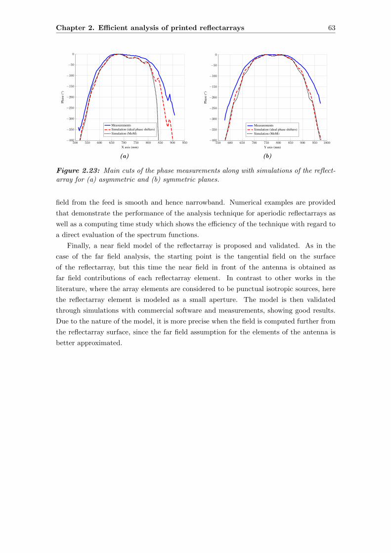
Chapter 2. Efficient analysis of printed reflectarrays 63
500 550 600 650 700 750 800 850 900 950−400
−350
−300
−250
−200
−150
−100
−50
0
X axis (mm)
Phas
e(°
)
MeasurementsSimulation (ideal phase shifters)Simulation (MoM)
(a)
550 600 650 700 750 800 850 900 950 1000−400
−350
−300
−250
−200
−150
−100
−50
0
Y axis (mm)
Phas
e(°
)
MeasurementsSimulation (ideal phase shifters)Simulation (MoM)
(b)
Figure 2.23: Main cuts of the phase measurements along with simulations of the reflect-array for (a) asymmetric and (b) symmetric planes.
field from the feed is smooth and hence narrowband. Numerical examples are provided
that demonstrate the performance of the analysis technique for aperiodic reflectarrays as
well as a computing time study which shows the efficiency of the technique with regard to
a direct evaluation of the spectrum functions.
Finally, a near field model of the reflectarray is proposed and validated. As in the
case of the far field analysis, the starting point is the tangential field on the surface
of the reflectarray, but this time the near field in front of the antenna is obtained as
far field contributions of each reflectarray element. In contrast to other works in the
literature, where the array elements are considered to be punctual isotropic sources, here
the reflectarray element is modeled as a small aperture. The model is then validated
through simulations with commercial software and measurements, showing good results.
Due to the nature of the model, it is more precise when the field is computed further from
the reflectarray surface, since the far field assumption for the elements of the antenna is
better approximated.


CHAPTER 3
Efficient pattern synthesis of
reflectarrays based on the Fast
Fourier Transform
3.1. Introduction
The design of directive reflectarrays with a pencil beam pattern is straightforward. Ac-
cording to the array theory [2], for the reflectarray to radiate in a direction (θ0, ϕ0), the
following progressive phase distribution should be achieved by the reflected tangential
field:
φ (xm, yn) = −k0 sin θ0 cosϕ0 xm − k0 sin θ0 sinϕ0 yn, (3.1)
where k0 is the free space wavelength and (xm, yn) the coordinates of the (m, n)th reflect-
array element center. Taking into account that the phase of the incident field from the
feed is −k0 di, with di the distance form the feed to each reflectarray element, the phase
distribution of the reflection coefficients that should be implemented by the reflectarray
elements is:
φR(xm, yn) = k0 (di − (xm cosϕ0 + yn sinϕ0) sin θ0) . (3.2)
In order to implement the phases of (3.2), the element dimensions (dipoles lengths, patches
dimensions, ...) are adjusted in such a way that the phase of the corresponding reflection
coefficient matches the required phase shift in the required polarization (phase of ρxx for
X polarization and ρyy for Y polarization).
However, when more complex radiation patterns are required, the use of a synthesis
algorithm is mandatory. For the reflectarray case, the synthesis of radiation patterns is
constrained by the radiation pattern of the feed, which fixes the amplitude of the inci-
dent field on each reflectarray element, and only the phase distribution can be modified.
The most typical approach for the reflectarray beam shaping is the Phase-Only Synthesis
(POS), whose output is the phase of the reflected field at each reflectarray element (or
equivalently, the phase of the reflection coefficients) that provides the required shaped
65

66 3.2. Intersection Approach for phase-only synthesis
beam. Then, the element dimensions will be adjusted to match the obtained phase distri-
bution, as commented above.
The algorithm described in this chapter for the synthesis of reflectarray antennas is the
Intersection Approach (IA), which in the most general case is described in [89] and can be
applied to any kind of antenna. However, due to the nature of the reflectarray antennas,
some particularizations can be made to the algorithm [94, 95] in order to take advantage
of the analysis based on the FFT, obtaining a very powerful algorithm while keeping a
very high numerical efficiency. This algorithm will be referred to as IA-POS. Since for
the POS case the most time consuming operation of the IA is the FFT, the algorithm
is very fast and allows the synthesis of very large reflectarrays in very short amounts of
time [2]. However, this version of the IA is based on a POS, so it only deals with copolar
patterns and there is no control over the crosspolar ones. Hence, a generalization of the
IA formulation for reflectarrays will be developed that includes crosspolar specifications.
This new formulation synthesizes a distribution of reflection coefficient matrices, instead
of phases, since to obtain the crosspolar pattern the full matrix is needed, as explained in
the previous chapter. This new algorithm will be denoted as IA-XP.
3.2. Intersection Approach for phase-only synthesis
The majority of pattern synthesis methods consists on the optimization of a functional
defined as an error function. However, there is a simpler understanding of the problem:
finding the intersection of two sets, or at least, the minor distance between them [89,95].
The IA is based on this approach and was first developed, in the case of antennas, for
arrays in which both amplitude and phase could vary along the surface of the antenna [94].
Although dynamics constraints have been implemented for array synthesis [145], where
several phase distributions were obtained with one amplitude distribution, reflectarrays
impose a tighter restriction, since the amplitude distribution is fixed by the incident field
from the feed and not by the synthesis process. Still, the IA developed for reflectarrays
provide excellent results for pattern synthesis.
The IA considers two sets: 1) the set of the radiation patterns that can be obtained
with the reflectarray (set R) and 2) the set of the radiation patterns that comply with
the requirements (set M) [89, 95]. Formally, both sets are sets of functions, which model
radiation patterns [94], although for clarity, only their radiation pattern nature will be
mentioned, as in [2]. Each iteration of the algorithm consists of a pair of operations,
namely forward (F) and backward (B) projections, as follows:
~Ei+1 = B[F(~Ei
)], (3.3)
where ~E is the radiated field by the antenna. The forward projection projects the far
field radiated by the antenna onto the set of far fields that comply with the specifications.
The backward projection projects the far field that fulfills the specifications onto the set
of far fields that can be radiated by the reflectarray. The aim of the sequence defined in
(3.3) is to find a radiation pattern that belongs simultaneously to both sets. If that is

Chapter 3. Efficient pattern synthesis of RA based on the FFT 67
M
R
x0
x∗
x0
x∗
F
B
F
BF
(a)
R Mx0
x∗
FB
FB
(b)
Figure 3.1: Sketch of the Intersection Approach between two sets for (a) one dimensionand (b) general case.
not possible because the intersection is empty, a radiation pattern should be found whose
distance to the set of patterns that fulfill the specifications is minimal [89]. Also, the IA is
a local optimizer and as such the starting point is of the utmost importance since it will
determine the correct convergence of the algorithm [89].
Figure 3.1(a) shows a sketch of the algorithm applied to one-dimensional sets. There,
x0 denotes the starting point of the algorithm and x∗ the solution reached. In this case,
the projection operators are the orthogonal projection of one curve to the other. As it
can be seen, depending on the starting point, the algorithm can reach a non-desired local
minima. Also, the steps provided by the algorithm become smaller as it reaches a solution
(not necessarily the optimum one).
A flow chart of the implemented algorithm is shown in Figure 3.2. The aim of the
algorithm is to obtain the phase distribution of the reflection coefficients that generates
the desired radiated field. Hence, the first step is to compute the far fields from the initial
reflected field, which can be one that generates a properly focused pencil beam [2]. After
that, the forward projection is divided into two steps. The template normalization will
define the synthesis as fixed or float gain, depending on how the templates are set. Then,
using the templates, the radiated field is projected onto the set of fields that comply with
the specifications.
Then, the backward projector is applied, which is divided in three steps. In the
first step, the reflected field is recovered applying the inverse transform to the one used
to compute the far fields. In general, the recovered reflected field will not be possible
to generate by the reflectarray antenna, so it will be projected onto the set of possible
radiation patterns (actually, possible reflected fields, but a possible reflected field generates
a possible radiation pattern) by imposing certain restrictions. Afterwards, the possible
radiated field is computed.
At this stage, the current computed far field is evaluated and depending on whether
it fulfills the specifications or not, the algorithm will continue to iterate or it will stop,
recovering the phase distribution from the last computed possible reflected field. Typically,

68 3.2. Intersection Approach for phase-only synthesis
Initialreflected field
Computation of theradiated field
Template Normalization
Projection onto the validradiation patterns set
Forward Projection(F)
~Ei
Reflected field recovery
Projection on the possibleradiation patterns
Computation of theradiated field
Backward Projection(B)
~E′i
Does thealgorithmconverge?
~Ei+1
Finalreflected field
YES
NO
Figure 3.2: Flow chart of the Intersection Approach for Phase-Only Synthesis.

Chapter 3. Efficient pattern synthesis of RA based on the FFT 69
convergence is achieved by imposing a minimum desirable error higher than zero, although
sometimes it is done by inspection of the current radiation pattern. Also, the algorithm
might diverge if the specifications are too restrictive or the starting point is not good
enough. In any case, the algorithm can be set to either stop when a minimum error is
accomplished or until a maximum number of iterations are reached. Details of the different
building blocks are discussed in the following sections.
3.2.1. Computation of the far field
The phase-only synthesis can be carried out either using the First or the Second Principles
of Equivalence. Although POS only deals with copolar requirements, the copolar pattern
is slightly different when computed and compared with both Principles, being the First
Principle more accurate than the Second. Here, the formulation for both Principles of
Equivalence will be presented for POS, starting with the Second Principle since its results
are necessary for the formulation with the First Principle.
However, the algorithms presented in this chapter can only work with the Second
Principle of Equivalence due to limitations in the formulation to recover the field at the
aperture from the far fields. This limitation and others will be overcome in future chapters
using more advanced algorithms, but the formulation for POS using both Principles will
be presented here for completeness.
3.2.1.1. Using the Second Principle of Equivalence
The computation of the far field radiated by a reflectarray antenna has been described
in detail in the previous chapter. Here, the process is the same in essence, but some
approximations have been assumed in order to adapt it to the synthesis process. The
reflected field was defined as
~EX/Yref (x, y) = E
X/Yref,x (x, y) x+ E
X/Yref,y (x, y) y, (3.4)
so the incident and reflected fields are related through the matrix Rmn as
~EX/Yref (xm, yn) = Rmn · ~EX/Y
inc (xm, yn). (3.5)
As discussed in the previous chapter, Rmn matrix includes the direct and cross coeffi-
cients for the two components of the incident field. Also, these components are complex
numbers and are different for each reflectarray element. However, for POS, ideal phase
shifters are considered, instead of real elements, and the cross polarization is not taken
into account. In this case, the reflection coefficient matrix is reduced to:
Rmn =
ejφmnxx 0
0 ejφmnyy
. (3.6)

70 3.2. Intersection Approach for phase-only synthesis
Thus, the reflected field can be expressed as
EX/Yref, x = ejφ
mnxx E
X/Yinc, x, (3.7a)
EX/Yref, y = ejφ
mnyy E
X/Yinc, y. (3.7b)
In (3.7) it is considered that no crosspolarization is produced by the element; but
there is another source of crosspolar radiation: the geometry. This crosspolarization is
produced due to the incidence angle of the polarization plane of the impinging wave on the
reflectarray element. However, it is interesting to have the synthesis process independent
for both polarizations, since modifying one dimension of the element affects more to the
corresponding polarization (such is the case, for instance, of patches or dipoles) in the
copolar pattern. Hence, the cross component of the incident wave is assumed to be zero
(y component in X polarization and x component in Y polarization), resulting in the
following reflected field components:
EXref, x = ejφ
mnxx EX
inc, x, (3.8a)
EYref, y = ejφ
mnyy EY
inc, y. (3.8b)
On the other hand, the spectrum functions were computed as two-dimensional IDFT.
Taken into account the reflected field of (3.8), the expressions for the spectrum functions
are
PXx (p, q) = Nx ·Ny ·K(p, q) ·K ′(p, q) · IDFT2
[EX
ref, x
], (3.9a)
P Yy (p, q) = Nx ·Ny ·K(p, q) ·K ′(p, q) · IDFT2
[EY
ref, y
], (3.9b)
where the constants K and K ′ were defined in (2.74) and (2.82) in (u, v) coordinates
and the change of variables to (p, q) was defined in (2.84). The steps for the efficient
computation of the IDFT2 with the FFT algorithm were also detailed in the previous
chapter.
Taking into account the spectrum functions of (3.9) and the Second Principle of Equiv-
alence, the θ and ϕ components of the far field for X polarization are
EXθ =
j k0 e−jk0r
2πrcosϕPX
x , (3.10a)
EXϕ = −j k0 e
−jk0r
2πrcos θ sinϕPX
x , (3.10b)
while for Y polarization the radiated fields are given by the equations
EYθ =
j k0 e−jk0r
2πrsinϕP Y
y , (3.11a)
EYϕ =
j k0 e−jk0r
2πrcos θ cosϕP Y
y . (3.11b)
Chapter 3. Efficient pattern synthesis of RA based on the FFT 71
Finally, applying Ludwig’s third definition of crosspolarization, the copolar and cross-
polar components are obtained using (2.61) and (2.62). For the case at hand, only the
copolar component is needed for both polarizations, which can be expressed as
EXcp =
j k0 e−jk0r
2πrPXx
(cos2 ϕ+ sin2 ϕ cos θ
), (3.12a)
EYcp =
j k0 e−jk0r
2πrP Yy
(sin2 ϕ+ cos2 ϕ cos θ
). (3.12b)
In classical implementations of pattern synthesis in array and reflectarray antennas,
only the array factor is taken into account to produce the required pattern shaping, assum-
ing that the effect of the element radiation pattern is negligible. However, in the present
implementation, the pattern synthesis is applied to the copolar far field of the antenna,
taking into account the constant K in (3.9), which accounts for the effect of the element
modeled as a small rectangular aperture (also known as active element pattern), instead of
an isotropic punctual source as is the case in the array factor. This methodology provides
more accuracy in the synthesis process.
3.2.1.2. Using the First Principle of Equivalence
The First Principle of Equivalence requires the computation of the reflected tangential
magnetic field. From the reflected field of (3.8) derived before, the magnetic field is
computed by applying (2.50)–(2.54) to (3.8), particularized for each polarization. For
polarization X, the reflected electric field has the following two components:
EXref, x = ejφ
mnxx EX
inc, x, (3.13a)
EXref, y = 0. (3.13b)
Thus, the z component according to (2.54) is
EXref, z = −
kref, xEXref, x
kref, z. (3.14)
The magnetic field is then obtained as:
~HXref(xm, yn) =
~kref × ~EXref(xm, yn)
ωµ0=
1
ωµ0
(kref, y E
Xref, z(xm, yn) x
−(kref, xE
Xref, z(xm, yn)− kref, z E
Xref, x(xm, yn)
)y
− kref, y EXref, x(xm, yn) z
).
(3.15)
As only the tangential magnetic field is needed, we finally have:
HXref, x =
kref, y EXref, z
ωµ0, (3.16a)

72 3.2. Intersection Approach for phase-only synthesis
HXref, y =
−kref, xEXref, z + kref, z E
Xref, x
ωµ0. (3.16b)
Notice that when using the Second Principle of Equivalence there was only one compo-
nent of the reflected electric field, and thus one spectrum function, per polarization after
applying the POS simplifications. This was convenient because this way the copolar far
field could be controlled independently for each polarization with the phase of one re-
flection coefficient, namely ρxx for X polarization and ρyy for Y polarization. However,
for the magnetic field there are now two components in the tangential field, and thus
two spectrum functions (having a total of three spectrum functions in the computation of
the far field with the First Principle of Equivalence, taking also into account the electric
field). Nevertheless, since the simplifications in the electric field apply, both components
of the tangential magnetic field only depend on one reflection coefficient, again ρxx for X
polarization and ρyy for Y polarization, maintaining the independence between the two
polarizations as with the other Equivalence Principle.
In the case of the Y polarization, the reflected electric field has the following compo-
nents:
EYref, x = 0, (3.17a)
EYref, y = ejφ
mnyy EY
inc, y. (3.17b)
Thus, the z component according to (2.54) is
EYref, z = −
kref, y EYref, y
kref, z. (3.18)
The magnetic field is then obtained as:
~HYref(xm, yn) =
~kref × ~EXref(xm, yn)
ωµ0
=1
ωµ0
((kref, y E
Yref, z(xm, yn)− kref, z E
Yref, y(xm, yn)
)x
− kref, xEYref, z(xm, yn) y − kref, xE
Yref, y(xm, yn) z
).
(3.19)
As only the tangential magnetic field is needed, we finally have:
HYref, x =
kref, y EYref, z − kref, z E
Yref, y
ωµ0, (3.20a)
HYref, y =
−kref, xEYref, z
ωµ0. (3.20b)
Once the tangential field has been obtained, the spectrum functions PXx , P Y
y , QX/Yx
and QX/Yy are computed following the steps provided in the previous chapter. Since for

Chapter 3. Efficient pattern synthesis of RA based on the FFT 73
the POS the spectrum functions PXy and P Y
x are zero, the simplified far fields for X
polarization are
EXθ =
jk0e−jk0r
4πr
[PXx cosϕ− η cos θ
(QX
x sinϕ−QXy cosϕ
)], (3.21a)
EXϕ = −jk0e
−jk0r
4πr
[PXx sinϕ cos θ + η
(QX
x cosϕ+QXy sinϕ
)], (3.21b)
while for Y polarization are
EYθ =
jk0e−jk0r
4πr
[P Yy sinϕ− η cos θ
(QY
x sinϕ−QYy cosϕ
)], (3.22a)
EYϕ = −jk0e
−jk0r
4πr
[−P Y
y cosϕ cos θ + η(QY
x cosϕ+QYy sinϕ
)]. (3.22b)
Finally, applying Ludwig’s third definition of crosspolarization, the copolar and cross-
polar components are obtained using (2.61) and (2.62). For the case at hand, only the
copolar component is needed for both polarizations, which can be expressed as
EXcp = cosϕEX
θ − sinϕEXϕ , (3.23a)
EYcp = sinϕEY
θ + cosϕEYϕ . (3.23b)
3.2.1.3. Differences between the First and Second Principles
When possible, the use of the First Principle of Equivalence for the analysis, synthesis
and design of reflectarray antennas is recommended since it provides more accurate re-
sults [43,88]. Although the main differences in the radiation patterns are in the crosspolar
component, there are also some differences in the copolar pattern.
Figure 3.3 shows the main cut of a shaped beam reflectarray with an isoflux pattern
which was synthesized using the IA-POS with the Second Principle of Equivalence. As
−80 −60 −40 −20 0 20 40 60 80
−15
−10
−5
0
5
10
15
20
θ (°)
Gain(dB)
1st Principle of Equivalence
2nd Principle of Equivalence
(a)
6 8 10 12 14 16 18 20 22 24 26 28 30 32 3416.5
17
17.5
18
18.5
19
19.5
θ (°)
Gain(dB)
1st Principle of Equivalence
2nd Principle of Equivalence
(b)
Figure 3.3: Differences in the copolar pattern of an isoflux beam shaped reflectarray forthe First and Second Equivalence Principles. (a) Cut in θ for ϕ = 0°. (b) Zoom in thecoverage area.

74 3.2. Intersection Approach for phase-only synthesis
it can be seen, the synthesized pattern correctly fulfills the template. However, if the
radiation pattern is computed using the First Principle of Equivalence and compared with
the pattern obtained with the Second Principle, there are some differences. The side lobes
present similar values for angles close to broadside, although they diverge for large angles.
More importantly, in the coverage area there is a drop in gain of about 0.23 dB at θ = 20°,
where the antenna is pointing. Even though the shape of the copolar gain would agree
with the template when computed with the First Principle, is notable that the predicted
gain is lower than with the Second Principle. Thus, it might be interesting to use the
POS formulation of the First Principle of Equivalence to synthesize reflectarrays whose
application demands a correct prediction of the gain, such as space applications [19, 20],
among others.
3.2.1.4. Inclusion of the dielectric frame
In the previous chapter the effect of the dielectric frame in the radiation patterns was
evaluated, and it was concluded that it was necessary to include it in the analysis since
the effects were important even in the copolar pattern. Hence, its inclusion in the synthesis
process is also recommended, along with the use of the First Principle of Equivalence, to
correctly synthesize the copolar pattern. However, when including the dielectric frame in
the synthesis, some considerations need to be taken into account.
First, the dielectric has to be analyzed with MoM beforehand in order to extract
the corresponding phase shift of the elements without metallizations that comprise the
dielectric frame. For this case, only the phases are needed since it is the only information
needed for POS, disregarding losses due to the dielectric and cross coefficients. And second,
the dielectric phases will remain unaltered during the whole synthesis process, since there
are no metallizations that will modify the phase shift introduced by the frame.
3.2.2. Forward projection
This projection is divided in two steps. First, the templates that give the requirements in
the copolar radiation patterns are normalized through a constant Cn. Then, the projection
in the set of the radiation patterns that fulfill the requirements is carried out.
3.2.2.1. Normalization of the requirement templates
The requirements of the copolar radiation patterns are usually given in gain. However,
the projection is carried out in radiated field units, so the following equation that relates
the gain and the radiated field must be used:
G(u, v) =|E(u, v)|2 2πr2
η0 Pfeed. (3.24)
Using (3.24), the gain templates are transformed to radiated field templates, resulting in
|Tmax(u, v)| =√Gmax(u, v) η0 Pfeed
2πr2, (3.25a)

Chapter 3. Efficient pattern synthesis of RA based on the FFT 75
|Tmin(u, v)| =√Gmin(u, v) η0 Pfeed
2πr2, (3.25b)
where Gmax and Gmin are the maximum and minimum requirement templates in copolar
gain, given in natural units; Pfeed the power given by the feed in watts, and Tmax and Tmin
the requirement field templates in natural units.
Now, two possibilities arise. The synthesis can be performed either in fixed or float
gain. If the synthesis is carried out in fixed gain, (3.25) are the final templates used in
the synthesis process. This method can be useful to further refine a previous synthesis, as
it will be shown in a subsequent chapter, devoted to crosspolar optimization. The other
possibility is to carry out the synthesis in float gain, which is the preferred method, since
it adapts automatically the templates to the maximum gain that can be obtained with
the antenna (reflectarray in this case). For the float gain synthesis, the templates are
normalized to the field radiated in a determined direction (u0, v0) which belongs to the
maximum gain region. Thus, a normalizing constant Cn is defined as
Cn =|Ecp(u0, v0)|
|Tav|, (3.26)
where Tav is the average value of the maximum and minimum templates in the desired
direction
Tav =Tcp,max(u0, v0) + Tcp,min(u0, v0)
2. (3.27)
The normalizing constant Cn is applied to the maximum and minimum templates in the
following fashion:
Tnmax(u, v) = Tmax(u, v) · Cn, (3.28a)
Tnmin(u, v) = Tmin(u, v) · Cn. (3.28b)
The normalization process is the same for both polarizations and different templates can
be used, as it would be the case of dual-polarized antennas with different shaped beams.
This normalization process defines a float gain synthesis where the middle point of the
templates at (u0, v0) is placed at the same level as the field. This method provides slightly
better results than the fixed gain synthesis where the templates are not normalized [95],
since it provides the shaping of the beam with the maximum gain that can be achieved
for the defined antenna dimensions.
3.2.2.2. Projection onto the set of valid radiation patterns
Once the templates have been conveniently normalized, the copolar component of the field
radiated by the reflectarray should accomplish
Tnmin(u, v) ≤ |Ecp(u, v)| ≤ Tn
max(u, v), (3.29)

76 3.2. Intersection Approach for phase-only synthesis
Tmin
Tmax
Tmin
Tmax
|Ecp|
Pr
Figure 3.4: Projection onto the set of valid radiation patterns.
for either polarization. This condition can be fulfilled by the Pr operator, defined for all
(u, v) for a generic electric field component as
Pr (E(u, v)) =
Tnmax(u, v) · arg (E(u, v)) , Tn
max(u, v) < |E(u, v)|
Tnmin(u, v) · arg (E(u, v)) , Tn
min(u, v) > |E(u, v)|
E(u, v), otherwise,
(3.30)
where arg (·) gives the phase of its complex argument. With this operator only the ampli-
tude of the field is changed. The phase remains unaltered. The result of this operation is
the field E′,
E′(u, v) = Pr (E(u, v)) . (3.31)
For the sake of simplicity, a generic E field component and template T were used in (3.30)
and (3.31), but they should be applied to the copolar component of both polarizations with
their respective normalized templates. This projection is shown graphically in Figure 3.4.
3.2.3. Backward projection
The backward projection (B), that is, the projection from the set of valid radiation patterns
(M) which fulfill the specifications, onto the set of possible radiation patterns (R), is
divided in three steps. First, the reflected field on the reflectarray surface is recovered, then
amplitude and phase constraints are imposed, and finally the possible radiation pattern is
computed.
3.2.3.1. Recovery of the reflected field
The first step in the implementation of the backward projection is the most complex,
since the inverse process of the computation of the radiated far fields has to be carried

Chapter 3. Efficient pattern synthesis of RA based on the FFT 77
out. Once the Pr operator in (3.30) is applied, a trimmed copolar far field is obtained.
Then, the spectrum functions can be directly recovered by isolating P in (3.12) using the
Second Principle of Equivalence, having
PXx = EX
cp
2πr
j k0 e−jk0r
1
cos2 ϕ+ sin2 ϕ cos θ, (3.32a)
P Yy = EY
cp
2πr
j k0 e−jk0r
1
sin2 ϕ+ cos2 ϕ cos θ. (3.32b)
In (3.32) there is a singularity when θ = π/2 rad and ϕ = π/2 rad for X polarization, and
θ = π/2 rad and ϕ = 0 rad for Y polarization, although it is in the limit of the visible
region in both cases (θ = π/2 rad). In order to avoid numerical instabilities (e.g. overflows
when θ → π/2 rad or divisions by zero), computations should avoid values of θ close to that
value. In any practical realization of the algorithm, this is easy to accomplish due to the
coarse discretization of the UV grid, which in most cases will not exceed from 512 × 512
or 1024× 1024 points.
Notice that isolating the P functions is possible since each equation in (3.12) only
has one variable using the Second Principle of Equivalence. However, this step of the
Backward Projection is not possible working with the First Principle of Equivalence, for
which each copolar pattern depends on three spectrum functions, Px or Py, depending
on the polarization, and Qx and Qy, as shown in (3.21) and (3.22). Thus, using the
First Principle it is not possible to recover the three spectrum functions from the copolar
component of the far field. This is the reason why the IA-POS must be implemented with
the Second Principle of Equivalence.
When calculating the far field from the reflected field, the spectrum function could
be expressed as 2D IDFT as in (3.9). At this point, it is straightforward to recover the
reflected field
EXref,x = DFT2
[PXx (p, q)
Nx ·Ny ·K(p, q) ·K ′(p, q)
], (3.33a)
EYref,y = DFT2
[P Yy (p, q)
Nx ·Ny ·K(p, q) ·K ′(p, q)
], (3.33b)
taking into account the change of variables described in (2.84).
3.2.3.2. Projection onto the set of possible radiation patterns
When the reflected field is recovered by (3.33), it is computed in a grid with the same
number of points as the far field, which is usually larger than the grid corresponding to the
reflectarray elements, as discussed in the previous chapter. Hence, the recovered field that
lies outside the reflectarray boundaries must be set to zero. This is an inherent constraint
of the algorithm derived from the fact that it uses the FFT to recover the reflected field.
In general, the amplitude of the recovered reflected field can take any value, even
values greater than the original reflected field, which cannot be accomplished by passive
reflectarrays. In fact, the amplitude of the reflected field is the same as the incident field

78 3.2. Intersection Approach for phase-only synthesis
(assuming no losses), and it remains fixed along the synthesis process. Hence, the next
constraint is to generate a reflected field with the amplitude of the incident field but the
phases of the recovered reflected field. This can be expressed mathematically through the
Pt operator as
Pt [Eref(xm, yn)] = |Einc(xm, yn)| · arg [Eref(xm, yn)] , (3.34)
which would be applied to recover the reflected field for both polarizations.
With the definition of the Pt operator in (3.34), only the phases are free to vary in
an entire 360° cycle in each iteration of the IA. This behavior is very useful in the first
stages of the synthesis process since a quick convergence can be obtained. However, when
a refinement is required, a wide variation in phase could be not recommended. In those
cases, the algorithm can be improved by introducing a phase constraint in the Pt operator,
limiting the maximum variation in phase with regard to the initial phase distribution.
Then, the Pt operator is modified as
Pt [Eref(xm, yn)] = |Einc(xm, yn)| · ejφ(xm, yn), (3.35)
where the phase term φ(xm, yn) is defined for each reflectarray element (m, n) depending
on the variation suffered during a cycle of the algorithm,
φ(xm, yn) =
arg (Eref(xm, yn)) ∀(m,n) / ∆φ(xm, yn) < ∆φmax,
arg (Eref,0(xm, yn)) + ∆φmax ∀(m,n) / ∆φ(xm, yn) ≥ ∆φmax,(3.36)
where
∆φ(xm, yn) = |arg (Eref(xm, yn))− arg (Eref,0(xm, yn))| , (3.37)
∆φmax is the maximum allowable phase variation and arg (Eref,0(xm, yn)) is the phase of
the reflected field at the starting point of the synthesis process. With the introduction of
this phase constraint, the convergence becomes slower, but a better control on the phase
distribution is obtained.
If the dielectric frame is taken into account in the synthesis process, the phases for the
elements belonging to the frame must not change at any iteration of the IA. Thus, the Pt
operator is further modified as
Pt [Eref(xm, yn)] =
|Einc(xm, yn)| · ejφ(xm, yn) / (m,n) /∈ diel. frame,
|Einc(xm, yn)| · ej arg(Eref,0(xm,yn)
)/ (m,n) ∈ diel. frame,
(3.38)
where φ(xm, yn) and arg (Eref,0(xm, yn)) are the same as before.
3.2.3.3. Computation of the radiated field
Finally, the backward projection is completed with the computation of the field radiated
by the reflectarray, considering the new reflected field distribution after applying the Pt
operator in (3.34), (3.35) or (3.38) on the recovered reflected field. This step has already

Chapter 3. Efficient pattern synthesis of RA based on the FFT 79
been described in Section 3.2.1, and for the IA-POS the Second Principle of Equivalence
must be used.
3.2.4. Variable number reduction
The starting point in the synthesis process is very important in order to avoid undesirable
convergence to local minima, since the IA is a local optimizer. The case of reflectarrays is
particularly critical, since the number of degrees of freedom can be very large (hundreds
or thousands of elements). Thus, a radiation pattern similar to the required one would
be desirable as a starting point. Another possibility is to start from a properly focused
pencil beam and to introduce some control in the optimization algorithm.
In order to improve the convergence of the synthesis method in the case of reflectarrays,
the number of unknowns should be reduced, reducing the number of degrees of freedom.
As a consequence, the number of local minima becomes lower and the convergence of the
algorithm is improved. This strategy can be carried out by a progressive synthesis of the
reflectarray from the center to the edges, which can be also explained as the variation
of the size of the reflectarray during the synthesis process (starting from an electrically
smaller antenna). This progressive synthesis can be carried out by changing the directivity
of the feed, starting from a high directivity feed. In this case, the field level at the edges
of the reflectarray is extremely low and only the elements at the center of the reflectarray
contribute significantly to the beam shaping. Although the physical size of the reflectarray
has not changed, the effective size is smaller. The effective size of the reflectarray is
progressively increased with the reduction of the feed directivity. The number of unknowns
is progressively increased in the algorithm, which is carried out through a number of steps,
avoiding undesired local minima. This technique can be easily implemented by modifying
the feed directivity, which in the case of an ideal cosq θ feed model is done varying the
q-factor of the function, starting with a high q value and ending with the q value which
models the required feed horn. This technique is referred to as a fictitious reduction of
unknowns.
3.2.5. Convergence criteria
The IA consists of an iterative approximation to the solution until a minimum is found.
The algorithm converges to a minimum, but it can be a local minimum. In fact, a con-
vergence to the global minimum is quite unlikely, especially when the starting point is
far from the required solution. In the algorithm, the last step of each iteration is the
evaluation of the convergence, treated as a distance. If the distance between the solutions
in two consecutive iterations of the algorithm is under a given threshold, the process is
falling in a local minima and it finishes. Thus, this criteria can be expressed as
‖|Ecp,i| − B [F (Ecp,i)]‖ = ‖|Ecp,i| − |Ecp,i+1|‖ < d. (3.39)
The norm function used to compute the distance between the solutions of two consec-

80 3.2. Intersection Approach for phase-only synthesis
utive iterations is defined as
‖f‖2 =∫∫
Ω|f(u, v)|2 du dv, (3.40)
where Ω is the UV area that belongs to the visible region. The double integral in (3.40)
can be easily implemented by a double summation since the UV grid is already discretized
to compute the radiation patterns.
3.2.6. Phase-only synthesis considerations
When performing phase-only synthesis, the only variables to be optimized are the phases
of the reflection coefficients ρmnxx and ρmn
yy . The approximations made to obtain the copolar
far field patterns using the tangential field of (3.8) have proven to be valid in the case
of reflectarray antennas [95], providing a copolar pattern which is very close to the exact
one.
Usually, the reflectarray is required to be placed at far field distance of the feed,
in which case the feed can be modeled as a cosq θ function [78], with very accurate re-
sults [19, 128]. This feed model can also be used in the preliminary steps of the synthesis
process and later use full wave simulations of the feed in order to accurately predict the
far field [20, 42, 146]. However, the copolar far fields obtained using both methods are
very similar between each other. In any case, the algorithm described in the present work
allows to use the real incident field from the feed, either by full wave simulations or near
field measurements. The incident field is fixed throughout the synthesis process and only
the phase shift that the reflectarray elements have to introduce is optimized in order to
obtain the required copolar pattern.
Due to the simplifications made on the Rmn matrix, the crosspolar pattern that could
be computed using (3.9) would not take into account the crosspolarization introduced by
the reflectarray elements, which in practice is an important contribution to the crosspolar
pattern. As it was explained before in detail, the copolar pattern obtained with the
simplifications applied to the Rmn matrix is still accurate. However, the crosspolar pattern
is not, hence a phase-only synthesis only deals with copolar requirements.
Once the synthesis is finished and the phases of ρmnxx and ρmn
yy are obtained, a design
can be carried out that takes into account the real element behavior. By using full wave
simulations based on local periodicity [29,54,76], the full Rmn matrix is computed, taking
into account mutual coupling between elements. During this step, a zero finding routine is
used that calls iteratively a full wave simulator to adjust the required phase shift for each
element. Because the synthesized phases are accurately adjusted using this procedure, the
resulting phase distribution will have a small error with regard to those obtained after the
POS, and hence the copolar pattern will be very close to the one synthesized.
3.2.7. Example
In this section, an application example of the IA will be shown for an isoflux pattern.
Since this pattern will be used in following chapters for other optimizations, a procedure

Chapter 3. Efficient pattern synthesis of RA based on the FFT 81
for its generation will be detailed.
3.2.7.1. Isoflux pattern
The goal of the isoflux pattern is to provide coverage with constant energy flux on the
surface of the Earth. A sketch of the Earth-satellite geometry is shown in Figure 3.5.
There, Re is the radius of the Earth, dmin and dmax are minimum and maximum distances
from the satellite to the Earth surface, and θmax the maximum coverage angle.
The attenuation curve due to free space propagation is given by the Friis formula [129]
A = 20 log (f) + 20 log (d) + 32.5, (3.41)
where A is the attenuation given in dB, f is the frequency in MHz and d is the distance
from the satellite to the surface of the Earth in Km. If (xs, ys) are the satellite coordinates
and (xe, ye) are the coordinates of a point in the Earth surface, d is calculated as
d =
√(xs − xe)
2 + (ys − ye)2. (3.42)
The distance from the satellite to the surface of the Earth is given by its orbit, so dmin
is known. Then, dmax is calculated using the Pythagorean theorem and θmax is obtained
as
cos θmax =dmax
dmin +Re. (3.43)
Considering the origin of coordinates the center of the Earth, the points of its surface
will follow the equation
x2 + y2 = R2e. (3.44)
Then, the linear equation from the satellite to a point in the surface of the Earth can be
expressed as
y = mx+ n, (3.45)
with m = − tan θ and n = −m (dmin +Re). Substituting (3.45) in (3.44), the following
quadratic equation is obtained:
(1 +m2)x2 + 2mnx−(R2
e − n2)= 0. (3.46)
By solving (3.46) two solutions are obtained, which correspond to the intersection of
θmax
Satellite
Earth
Re
Redmin
dmax
θ d x
y
Figure 3.5: Sketch of the Earth-satellite geometry.

82 3.2. Intersection Approach for phase-only synthesis
the straight line d with the Earth circumference. The one with x < 0, according to
Figure 3.5, is selected; and then y is obtained with (3.44). This solution corresponds to
the point (xe, ye) in (3.42), which along with the known satellite position (xs, ys) enable
the calculation of the attenuation given by (3.41).
The attenuation curve is computed in a single plane, but since it is symmetric in ϕ,
it is straightforward to obtain the attenuation in the whole Earth surface in spherical
coordinates. It is common to perform reflectarray synthesis in the UV plane [2], knowing
that u = sin θ cosϕ and v = sin θ sinϕ.
The obtained attenuation pattern can be used directly as radiation pattern template
if a symmetric antenna geometry is used. Apart from the attenuation curve, side lobe
levels, ripple and a transition zone should also be specified. However, it is more common
to use single-offset configurations [2], such as the one shown in Figure 2.1. The reflectarray
radiates at an angle θ = θ0 with regard to its own coordinate system, RCS. Hence, the
centered templates have to be rotated by applying a proper transformation.
The template for the centered configuration in (θ, ϕ) coordinates is referenced to the
RCS (xr, yr, zr) of Figure 2.1. Each point of the template is transformed from spherical
coordinates to cartesian coordinates
xra = sin θra cosϕra, (3.47a)
yra = sin θra sinϕra, (3.47b)
zra = cos θra, (3.47c)
and then the following transformation is appliedxant
yant
zant
=
cos θ0 0 sin θ0
0 1 0
− sin θ0 0 cos θ0
xra
yra
zra
. (3.48)
Then, the cartesian coordinates will be transformed to spherical coordinates and from
there to UV coordinates, with the usual operations.
3.2.7.2. Antenna specifications
The reflectarray is made up of 1528 elements disposed in a regular circular grid of 44× 44
cells. The working frequency is 30 GHz and the periodicity is 4 mm× 4 mm (0.4λ). The
reflectarray is fed by a horn antenna whose phase center is placed at (−40, 0, 195) mm
with regard to the reflectarray coordinate system (see Figure 2.1). The feed is modeled
as a cosq θ function following [78] with a q-factor of 14.8, which produces an illumination
taper of −12 dB at the reflectarray edges. The requirements for the isoflux pattern are
specified by a reflectarray with θ0 = 20°, side lobe level of −19 dB and 0.25 dB of allowable
ripple, placed on a satellite in geostationary orbit.

Chapter 3. Efficient pattern synthesis of RA based on the FFT 83
0.5 1 1.5 2 2.5 3 3.5 4−300
−200
−100
0
100
Patch length (mm)
Phase
(°)
θ = 0°, ϕ = 0°θ = 20°, ϕ = 15°θ = 30°, ϕ = 40°
(a)
0.5 1 1.5 2 2.5 3 3.5 4−300
−200
−100
0
100
Patch length (mm)
Phase
(°)
29 GHz30 GHz31 GHz
(b)
Figure 3.6: Phase range of the unit cell as a function of patch length for a periodicity of0.4λ at 30 GHz. (a) For different incidence angles at 30 GHz. (b) For different frequenciesat (θ, ϕ) = (20°, 15°).
3.2.7.3. Unit cell study
The reflectarray chosen element is the rectangular microstrip patch backed by a ground
plane [147]. Since only a single layer is used, the provided phase range of the cell will be
lower than 360° [2]. Hence, it is important to study the element in order to delimit the
phase range as a function of the patch size.
The Arlon 25N substrate is selected, with a relative permittivity εr = 3.38, thickness
h = 18 mil and loss tangent tan δ = 0.0025 at 10 GHz. Figure 3.6 shows the phase
variation of the unit cell as a function of the patch length for different angles of incidence
and frequencies. In this study, the patches are squares. The results show that, in this
particular case, the incidence angle barely affects the phase shift introduced by the element.
When the frequency is shifted, the phase variation is non-linear, since for dimensions lower
than 2 mm and higher than 3 mm it barely changes, but between 2 and 3 mm the phase
is shifted with frequency.
In order to maximize the available phase range avoiding extreme values of the patch
lengths (which would compromise the local periodicity assumption when carrying out the
design [2]), the patch length is restricted to vary in the range 1.7 to 3.2 mm, which provides
a phase range of about 300°.
3.2.7.4. Pattern synthesis and design
The reflectarray synthesis is carried out with the IA algorithm in several stages as described
before, starting with a high value of q in order to artificially reduce the number of variables.
Each step of the synthesis reduces the q-factor until its value reaches that of the horn feed.
The starting point is a pencil beam pattern pointing at (θ, ϕ) = (20°, 0°). Also, since the
generation of the isoflux template is parameterized, in the first steps of the synthesis
the allowed ripple will be higher in order to facilitate convergence, and as the algorithm is
approaching the solution, the ripple will be gradually reduced until the prescribed template
value is achieved. Table 3.1 shows the number of iteration for each q-factor at each step
of the synthesis of the isoflux pattern.
Since the selected unit cell only provides a phase range of 300°, the IA needs to be
modified in order to impose a phase range restriction. In the general framework of the
IA applied to array synthesis, the reflectarray is a particular case in which the amplitude

84 3.2. Intersection Approach for phase-only synthesis
Table 3.1: Number of iterations for each q-factor and its associated taper at each step ofthe synthesis of the isoflux pattern.
q-factor Taper (dB) # it.
80 60.0 20
60 45.3 40
50 38.0 40
40 30.6 50
30 23.2 60
20 15.9 30
15 12.2 60
14.8 12.0 130
is fixed by the incident field of the feed, and now the phase is also constrained in order
to match the available phase range from the unit cell, allowing it to vary only from 0° to
−300° to match the provided phase shift by the unit cell, shown in Figure 3.6.
Once the synthesis is finished and the required phase distribution is obtained, the
patch lengths are adjusted element by element using the Method of Moments (MoM) [54]
and a zero-finding routine. In this process, the real angle of incidence from the feed
to each element of the reflectarray is used, in order to take into account possible phase
shifts due to the incidence angle. Also, the MoM employs the Floquet theorem to analyze
the unit cell, which embeds the analyzed element within an infinite array comprised of
the same element, taking into account mutual coupling and the reflected field from the
ground. It is thus important that the patch size variation is smooth in order to fulfill
the local periodicity assumption of the analysis technique. Also, the design produces
slightly rectangular patches, since the reflection coefficients are to some extent different
for both polarizations, and the synthesized phases for both polarizations are not completely
identical.
3.2.7.5. Results
The synthesis was carried out for both polarizations, obtaining a dual-linear polarized
reflectarray with an isoflux pattern in both polarizations. The results for both polarizations
are similar, and only the patterns for X polarization are shown. Figure 3.7 shows the
synthesized phases with a total phase range of 300° imposed during the synthesis process.
As reference, a synthesis with no phase constraints was also performed with the phase
distributions shown in Figure 3.8.
Figure 3.9 shows the results between the synthesis with and without phase constraints.
When the phase is free to vary in the whole 360° range, a smooth coverage area can be
obtained. However, restricting the phase range to 300° causes the algorithm not to converge
properly, and there is a ripple in the coverage zone. It is also shown the simulation after
the design was made, simulating the patches with MoM [54], and there is little variation
in the copolar component with regard to the simulation with ideal phase shifters.
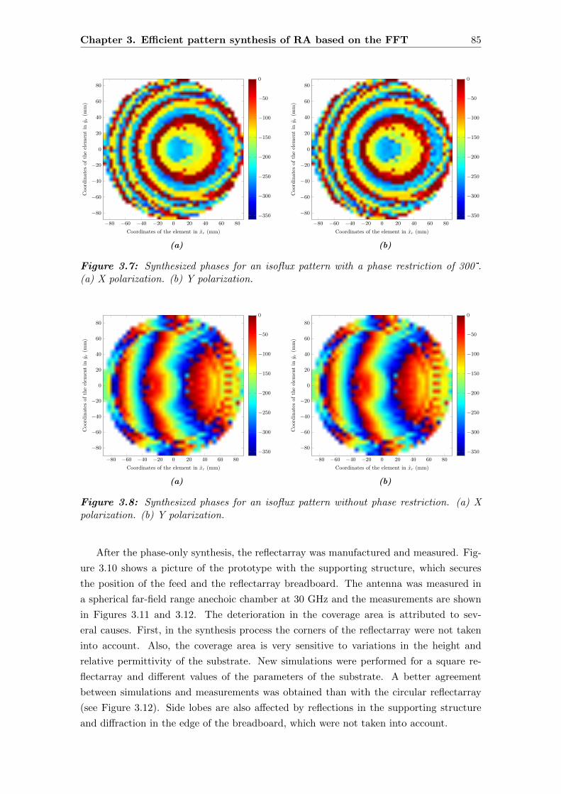
Chapter 3. Efficient pattern synthesis of RA based on the FFT 85
−80 −60 −40 −20 0 20 40 60 80
−80
−60
−40
−20
0
20
40
60
80
Coordinates of the element in xr (mm)
Coordinates
oftheelem
entin
y r(m
m)
−350
−300
−250
−200
−150
−100
−50
0
(a)
−80 −60 −40 −20 0 20 40 60 80
−80
−60
−40
−20
0
20
40
60
80
Coordinates of the element in xr (mm)
Coordinates
oftheelem
entin
y r(m
m)
−350
−300
−250
−200
−150
−100
−50
0
(b)
Figure 3.7: Synthesized phases for an isoflux pattern with a phase restriction of 300°.(a) X polarization. (b) Y polarization.
−80 −60 −40 −20 0 20 40 60 80
−80
−60
−40
−20
0
20
40
60
80
Coordinates of the element in xr (mm)
Coordinates
oftheelem
entin
y r(m
m)
−350
−300
−250
−200
−150
−100
−50
0
(a)
−80 −60 −40 −20 0 20 40 60 80
−80
−60
−40
−20
0
20
40
60
80
Coordinates of the element in xr (mm)
Coordinates
oftheelem
entin
y r(m
m)
−350
−300
−250
−200
−150
−100
−50
0
(b)
Figure 3.8: Synthesized phases for an isoflux pattern without phase restriction. (a) Xpolarization. (b) Y polarization.
After the phase-only synthesis, the reflectarray was manufactured and measured. Fig-
ure 3.10 shows a picture of the prototype with the supporting structure, which secures
the position of the feed and the reflectarray breadboard. The antenna was measured in
a spherical far-field range anechoic chamber at 30 GHz and the measurements are shown
in Figures 3.11 and 3.12. The deterioration in the coverage area is attributed to sev-
eral causes. First, in the synthesis process the corners of the reflectarray were not taken
into account. Also, the coverage area is very sensitive to variations in the height and
relative permittivity of the substrate. New simulations were performed for a square re-
flectarray and different values of the parameters of the substrate. A better agreement
between simulations and measurements was obtained than with the circular reflectarray
(see Figure 3.12). Side lobes are also affected by reflections in the supporting structure
and diffraction in the edge of the breadboard, which were not taken into account.

86 3.3. Efficient generalization of the IA with FF XP requirements
−1 −0.8 −0.6 −0.4 −0.2 0 0.2 0.4 0.6 0.8 1−30
−25
−20
−15
−10
−5
0
v
Normalized
pattern
(dB)
No phase const.Ideal phase shiftersPatches
−0.2 −0.1 0 0.1 0.2
0
−0.25
−0.5
−0.75
−1
(a)
−1 −0.8 −0.6 −0.4 −0.2 0 0.2 0.4 0.6 0.8 1−30
−25
−20
−15
−10
−5
0
u
Normalized
pattern
(dB)
No phase const.Ideal phase shiftersPatches
0.1 0.2 0.3 0.4 0.5
0
−0.25
−0.5
−0.75
−1
(b)
Figure 3.9: Main cuts of the synthesized isoflux pattern for three different simulations forX polarization: reference simulation (no phase constraints, red solid), simulation with idealphase shifters (phase constraints, dashed black) and design simulation (phase constraints,dotted green). (a) u = 0.34. (b) v = 0.
Figure 3.10: Picture of the prototype in the anechoic chamber.
These issues can be minimized by choosing a more appropriate antenna geometry,
which reduces the interference of the supporting structure, and by employing a rectangular
reflectarray instead of a circular one, having more variables to adjust the pattern and
taking into account the corners of the breadboard. Also, decreasing the illumination at
the edge would reduce the diffraction effects.
3.3. Efficient generalization of the Intersection Approach
with far field crosspolar requirements
The main disadvantage of the Intersection Approach algorithm presented in the previous
section is that it only performs a phase-only synthesis, which means that it only deals
with the copolar pattern and there is no control over the crosspolar one. One of the first
attempts to reduce the crosspolar radiation pattern in reflectarrays was presented in [114]
and later used in [115]. It is based on properly adding a constant to the reflectarray phase

Chapter 3. Efficient pattern synthesis of RA based on the FFT 87
−1 −0.8 −0.6 −0.4 −0.2 0 0.2 0.4 0.6 0.8 1−1
−0.8
−0.6
−0.4
−0.2
0
0.2
0.4
0.6
0.8
1
u
v
−20
−18
−16
−14
−12
−10
−8
−6
−4
−2
0
(a)
−1 −0.8 −0.6 −0.4 −0.2 0 0.2 0.4 0.6 0.8 1−1
−0.8
−0.6
−0.4
−0.2
0
0.2
0.4
0.6
0.8
1
u
v
−40
−35
−30
−25
−20
−15
−10
−5
0
(b)
Figure 3.11: 3D measured pattern for X polarization. (a) Copolar. (b) Crosspolar.
−1 −0.8 −0.6 −0.4 −0.2 0 0.2 0.4 0.6 0.8−30
−25
−20
−15
−10
−5
0
u
Normalized
pattern
(dB)
Sim. 30 GHz. circ., Er=3.38, h=18milSim. 30 GHz. circ., Er=3.38, h=16milSim. 30 GHz. circ., Er=3.28, h=18milSim. 30 GHz. sq., Er=3.38, h=18milSim. 30 GHz. sq., Er=3.38, h=16milSim. 30 GHz. sq., Er=3.28, h=18milMeasured CP 30 GHz.Measured XP 30 GHz.
0.15 0.2 0.25 0.3 0.35 0.4 0.45 0.5
0
−1
−2
−3
−4
Figure 3.12: Measurement and simulations for v = 0 for X polarization.
distribution in order to enforce 180° phase shifts and amplitude nulls in the reflection cross
coefficients that contribute more to the crosspolar pattern. However, it is not flexible since
it only tries to reduce the contribution of the cross coefficients after the synthesis is done
instead of synthesizing the crosspolar pattern to a desired value. This latter approach
was followed in [116–118], using the IA general framework [89] with the Broyden-Fletcher-
Goldfarb-Shanno (BFGS) [100] algorithm as the backward projector. It directly optimized
the geometry of the antenna using MoM, resulting in a very slow algorithm. Also, it only

88 3.3. Efficient generalization of the IA with FF XP requirements
dealt with single-polarized reflectarrays. More recently, some works have appeared that
deal with dual-polarized reflectarrays with crosspolar constraints. For instance, in [17],
a faceted dual-polarized reflectarray with crosspolar suppression is presented, where after
a POS pattern is obtained, the crosspolar component is suppressed and the currents on
the surface of the reflectarray are obtained. From there, the matrix of reflection coeffi-
cients are computed, which fully characterize the reflectarray element. In [18] another
faceted reflectarray is designed using a different approach. The reflectarray is directly
optimized [119] using a gradient-based minimax algorithm and it also uses a phase-only
synthesis as starting point, but in this case the initial reflectarray phase distribution is
retrieved from a shaped reflector design.
In this section, a generalization of the IA algorithm presented in the previous sec-
tion is developed for the synthesis of planar dual-polarized reflectarrays with crosspolar
requirements. It will be denoted as IA-XP. As in [17], it synthesizes the matrix of com-
plex reflection coefficients, although in a more flexible fashion since it is based on the IA
framework of [116–118], allowing to perform the synthesis in one step without requiring a
previous POS (although a previous POS would improve the starting point, which could
improve the convergence of the algorithm as in any local optimizer [89]), and allowing
the design of dual-polarized antennas while preserving the algorithm efficiency by using
the FFT in both projections. In contrast with POS, where the phases are free to take
any value, the matrices of reflection coefficients might take values which are impossible
to obtain with passive reflectarrays. Hence, a lossless and lossy passive two-port network
analysis of the reflectarray unit cell is carried out as part of an effort to impose constraints
to obtain feasible reflection coefficients for passive reflectarrays. From this study, the re-
striction equations are derived for both cases involving reflection coefficient amplitudes
and phases. Numerical examples are provided that show the capabilities of the algorithm
to synthesize reflection coefficients with restrictions.
For this generalization, the IA framework remains the same, and it is based on the
iterative process described by (3.3). Also, the same flow chart as the one shown in Fig-
ure 3.2 still applies. The difference lies in the redefinition of both projectors (namely, the
forward F and backward B projectors) to include the crosspolar requirements. Despite
this redefinition, the divisions in different steps of each projector remain the same as well.
However, the IA-XP also presents the limitation that must be implemented with the Sec-
ond Principle of Equivalence for the computation of the far field, since using the First
Principle would not allow to recover the reflected field using the FFT in the backward
projector, as it happened in the case of the IA-POS.
3.3.1. Computation of the far field
A detailed description of the computation of the far field radiated by a reflectarray antenna
has already been described in the previous chapter using the First and Second Principles
of Equivalence. However, as it happened in the POS case, only the Second Principle
is suitable for this algorithm, as it will be shown later on. For the POS case, some
simplifications in the Rmn matrix were applied, in which the reflectarray elements were

Chapter 3. Efficient pattern synthesis of RA based on the FFT 89
considered as ideal lossless phase shifters; as well as others in the reflected field. As
a result, only the copolar pattern could be considered in the synthesis process and the
two polarizations were synthesized independently from each other. In order to include
crosspolar requirements it is necessary to use the full Rmn matrix, with no simplifications.
This way, the cross coefficients are not zero, and account for an important contribution to
the crosspolar pattern. Then, the reflected field at each element (m,n) is given by
~EX/Yref (xm, yn) = Rmn · ~EX/Y
inc (xm, yn), (3.49)
with
Rmn =
ρmnxx ρmn
xy
ρmnyx ρmn
yy
, (3.50)
and ~EX/Yinc the incident field from the feed. Equation (3.49) provides the relation between
the reflected field on the surface of the reflectarray with the incident field from the feed
through the matrix of reflection coefficients for each element of the reflectarray. The
reflected field can be also expressed as
~EX/Yref (x, y) = E
X/Yref,x (x, y) x+ E
X/Yref,y (x, y) y, (3.51)
taking into account that the desired component for a given polarization X or Y is the x
or y component, respectively.
Once the total tangential field has been obtained, the far field radiated by the antenna is
computed. Using the Second Principle of Equivalence, the far field in spherical coordinates
is given by [85]
EX/Yθ =
jk0e−jk0r
2πr
(PX/Yx cosϕ+ PX/Y
y sinϕ), (3.52a)
EX/Yϕ = −jk0e
−jk0r
2πrcos θ
(PX/Yx sinϕ− PX/Y
y cosϕ), (3.52b)
with PX/Yx and P
X/Yy being the spectrum functions. It is worth noting that when the
synthesis process is carried out only for the copolar pattern (POS case), the simplifica-
tions in the reflected field cause that the far fields for both polarizations only require the
computation of one spectrum function, Px for X polarization and Py for Y polarization
(see (3.10), (3.11) and (3.12)). However, now both functions are necessary since also the
crosspolar pattern has to be accurately computed. They can be calculated as
PX/Yx (u, v) =
∫∫SE
X/Yref,x (x, y) e
jk0(ux+vy) dx dy, (3.53a)
PX/Yy (u, v) =
∫∫SE
X/Yref,y (x, y) e
jk0(ux+vy) dx dy, (3.53b)
where S is the surface of the planar aperture. The calculation of Px and Py is the most time
consuming problem in the computation of the radiated field. A direct evaluation of (3.53)

90 3.3. Efficient generalization of the IA with FF XP requirements
gives a time complexity of O(M2), being M the number of points of the grid in the UV
space. However, they can be expressed as a two-dimensional inverse Fourier transform
and thus calculated efficiently by means of a two-dimensional inverse FFT (IFFT) with a
time complexity of O(M logM) as follows:
Px = NxNyKK ′ IFFTEref,xe
−jπ(m+n), (3.54a)
Py = NxNyKK ′ IFFTEref,ye
−jπ(m+n), (3.54b)
where Nx and Ny are the number of elements in the x and y directions, respectively; m
and n integer indices of the reflectarray elements, K ′ is a phase-only term and K the
amplitude of a single element radiation pattern. The detailed development was shown in
the previous chapter.
Once the radiated far field is obtained with (3.52), the copolar and crosspolar compo-
nents are obtained applying Ludwig’s third definition of crosspolarization starting from
the θ and ϕ components [131]. They are defined in the case of X polarization as EXcp
EXxp
=
cosϕ − sinϕ
− sinϕ − cosϕ
EX
θ
EXϕ
, (3.55)
and for Y polarization as EYcp
EYxp
=
sinϕ cosϕ
cosϕ − sinϕ
EY
θ
EYϕ
. (3.56)
3.3.2. Forward projection
The forward projection is again divided in two steps. The first step consists in the normal-
ization of the templates that provide the requirements in copolar and crosspolar radiation
patterns, which are usually given in gain. Hence, in order to carry out the synthesis, the
gain templates must be converted to field templates, which can be simply done by taking
the square root of the gain in natural units, as in (3.25) for the IA-POS. The templates
are then normalized to the field radiated value in a determined direction (u0, v0) which
belongs to the maximum gain region. Thus, a normalizing constant is defined as follows:
Cn =|Ecp(u0, v0)|
|Tav|, (3.57)
where Tav is the average value of the maximum and minimum templates in the desired
direction
Tav =Tcp,max(u0, v0) + Tcp,min(u0, v0)
2. (3.58)

Chapter 3. Efficient pattern synthesis of RA based on the FFT 91
The normalizing constant Cn has to be defined for both polarizations and is to be applied
to both copolar and crosspolar templates in the following fashion
Tncp,max(u, v) = Tcp,max(u, v) · Cn, (3.59a)
Tnxp,max(u, v) = Txp,max(u, v) · Cn. (3.59b)
In the same way to (3.59), the minimum templates also have to be normalized. The
normalization process is the same for both polarizations and different templates can be
used, as it would be the case of dual-polarized antennas with different shaped beams. This
normalization process defines a float gain synthesis where the middle point of the templates
at (u0, v0) is placed at the same level as the field. This method provides slightly better
results than the fixed gain synthesis where the templates are not normalized. With regard
to the IA-POS, notice that Cn is computed only with the copolar field and templates, but
is now applied to both copolar and crosspolar templates.
Once the templates have been normalized, both components of the radiated field should
accomplish the following condition:
Tncp,min(u, v) ≤ |Ecp(u, v)| ≤ Tn
cp,max(u, v), (3.60a)
Tnxp,min(u, v) ≤ |Exp(u, v)| ≤ Tn
xp,max(u, v). (3.60b)
This condition can be fulfilled by the Pr operator, defined for all (u, v) as follows for a
generic electric field component E:
Pr (E(u, v)) =
Tnmax(u, v) · arg (E(u, v)) , Tn
max(u, v) < |E(u, v)|
Tnmin(u, v) · arg (E(u, v)) , Tn
min(u, v) > |E(u, v)|
E(u, v), otherwise,
(3.61)
where arg (·) gives the phase of its complex argument. With this operator only the ampli-
tude of the field is changed. The phase remains unaltered. The result of this operation is
the field E′,
E′(u, v) = Pr (E(u, v)) . (3.62)
For the sake of simplicity, a generic E field component and template T were used in (3.61)
and (3.62), but they should be applied to the copolar and crosspolar components of both
polarizations with their respective normalized templates. The result of the forward pro-
jection, E′(u, v) given by (3.62), is a radiation pattern that fulfills the specifications but
which, in general, cannot be radiated by the antenna (it belongs to the set M).
3.3.3. Backward projection
The backward projection is implemented in three steps. First, the reflection coefficient
matrices must be recovered. Starting from the trimmed copolar and crosspolar components
according to Ludwig’s third definition, the θ and ϕ components of the far field have to

92 3.3. Efficient generalization of the IA with FF XP requirements
be calculated. As the matrices that relate the θ and ϕ components with the copolar and
crosspolar components in (3.55) and (3.56) are symmetric and orthogonal, their inverses
are equal to themselves, so the far fields in spherical coordinates are easily obtained for
both polarizations.
Now, the spectrum functions must be obtained from Eθ and Eϕ. Re-expressing (3.52)
in matrix form and calculating the inverse, Px and Py are found PX/Yx
PX/Yy
=2πr
jk0e−jk0r
cosϕ − sinϕ/ cos θ
sinϕ cosϕ/ cos θ
EX/Yθ
EX/Yφ
. (3.63)
In (3.63) there is a singularity when θ = π/2 rad, although it is in the limit of the visible
region. In order to avoid numerical instabilities (e.g. overflows when θ → π/2 rad or divi-
sions by zero), computations should avoid values of θ close to that value. In any practical
realization of the algorithm, this is easy to accomplish due to the coarse discretization of
the UV grid, which in most cases will not exceed from 512× 512 or 1024× 1024 points.
As it happened with the IA-POS, recovering the spectrum functions is not possible
when using the First Principle of Equivalence since there would be four spectrum functions
per polarization, and only two far field components, having an underdetermined system
with infinite solutions.
When calculating the far field from the reflected field, the spectrum functions could
be expressed as 2D IFFT as in (3.54). At this point it is straightforward to recover the
reflected field
Eref,x = FFT Px/NxNyKK′ ejπ(m+n), (3.64a)
Eref,y = FFT Py/NxNyKK′ ejπ(m+n). (3.64b)
The FFT recovers the reflected field in a grid with the same number of points as the UV
grid. If this grid has more points than the actual reflectarray (i.e. to have better resolution
of the radiated far fields), all the points of the recovered reflected field outside the physical
reflectarray must be set to zero. This is an inherent constraint of the intersection approach
algorithm and prevents it to converge in just one iteration when no other constraints are
imposed. This also happened in the IA-POS.
Once the reflected field is recovered, along with the incident field, the reflection co-
efficients are recovered. Four equations can be extracted from (3.49), two for each po-
larization. As the unknowns are also four (the four reflection coefficients), one solution
is obtained for dual-polarized antennas. This means that both polarizations are not in-
dependent anymore (as in contrast to the phase-only synthesis) in this version of the IA
algorithm. The recovered reflection coefficients correspond to the Floquet fundamental
mode when analyzed with an electromagnetic technique [2]. The solution to (3.49) is
ρxy =EY
ref,x · EXinc,x − EX
ref,x · EYinc,x
EYinc,y · EX
inc,x − EXinc,y · EY
inc,x
, (3.65a)
Chapter 3. Efficient pattern synthesis of RA based on the FFT 93
ρxx =EX
ref,x · EYinc,y − EY
ref,x · EXinc,y
EYinc,y · EX
inc,x − EXinc,y · EY
inc,x
, (3.65b)
ρyx =EY
ref,y · EXinc,y − EX
ref,y · EYinc,y
EYinc,x · EX
inc,y − EXinc,x · EY
inc,y
, (3.65c)
ρyy =EX
ref,y · EYinc,x − EY
ref,y · EXinc,x
EYinc,x · EX
inc,y − EXinc,x · EY
inc,y
. (3.65d)
The second step in the implementation of the backward projection is to impose con-
straints on the reflection coefficients. After solving for the reflection coefficients, the solu-
tion can give any value, in general with magnitudes (modulus) greater than one. Hence,
some constraints have to be applied. The magnitudes must be smaller than one and the
reflection coefficients have to meet the power balance. However, the more constraints there
are the more difficult for the algorithm to converge. Furthermore, the fact that both polar-
izations are not independent from each other anymore reduces the degrees of freedom thus
making it harder to converge and control. In the following section, restriction equations
are derived in order to obtain feasible reflection coefficients for passive reflective elements
when constraints are applied in this step of the backward projection. In addition to those
constraints, if the dielectric frame is considered during the synthesis with the IA-XP, the
reflection coefficient matrix of those elements must remain unchanged at each iteration.
Those matrices should be computed using MoM before the first iteration of the algorithm
in order to take into account the real effect of a dielectric frame.
Finally, the third step consists in the computation of the radiated far fields from the
reflection coefficients and the incident field, as detailed previously. If the far fields fulfill
the specifications (or are close enough), the synthesis process concludes. Otherwise, the
iterative process continues by applying the forward projection, and then again the back-
ward projection until a minimum user-defined error is achieved or a determined number
of iterations reached. In this regard, the IA-POS convergence criteria of Section 3.2.5 is
the same for the IA-XP, but integrating the four far fields in the visible region instead of
only the two copolar components.
3.3.4. Efficiency of the algorithm
The presented algorithm is very efficient. Each iteration of the IA is comprised of one
forward and one backward projection. The most expensive operation in each projection
is the FFT/IFFT, with a time complexity of O(M logM). Each projection has four calls
to the FFT, since it has to compute four different radiation patterns, which makes a
total of eight calls to the FFT. This is extremely fast in modern computers. Tests were
carried out in an Intel Core i3-2100 with 4 CPU (two physical, two virtual) at 3.1 GHz,
taking less than 0.5 s each iteration for a UV grid of 512 × 512 points. As for any local
optimizer, convergence to a suitable solution depends on the starting point, specifications
and antenna geometry [89].
94 3.3. Efficient generalization of the IA with FF XP requirements
3.3.5. Feasibility of the R matrix
When synthesizing radiation patterns with the algorithm described above, some restric-
tions have to be imposed depending on the antenna under consideration. For the case of
passive reflectarrays, the reflected power will be at best equal to the incident power, when
no losses are considered. This means that the magnitudes of the reflection coefficients
cannot be greater than one, in natural units. However, imposing this condition does not
mean that the obtained reflection coefficients after the synthesis process are feasible. The
power balance must be met and perhaps other conditions.
Each cell of the reflectarray can be seen as a two port network, being port 1 the x
component and port 2 the y component of the electric field. Both ports share the same
physical space but are orthogonal to each other. A schematic view of this network is
shown in Figure 3.13. This analogy is only valid on the surface of the cell, where the
reflection coefficients are defined [2]. From this point of view, the incident and reflected
fields are related through the Rmn matrix. However, in order to carry out the feasibility
analysis considering the cell as a two port network an S-parameter matrix is needed [148],
and Rmn is not an S-parameter matrix. As the characteristic impedances are unknown in
Cartesian basis, it is best to carry out the analysis in the TE-TM basis.
3.3.5.1. Obtaining matrix S from matrix R
The relation between the TE-TM and Cartesian components for the fundamental Floquet
harmonic is [2]
eTE = − sinϕ x+ cosϕ y, (3.66a)
eTM = cosϕ x+ sinϕ y, (3.66b)
where (θ, ϕ) is the angle of incidence of the fundamental mode at each reflectarray element.
Equation (3.66) is the equation system to change from Cartesian to TE-TM basis. The
CELL
Einc,x
Eref,x
Port 1
Einc,y
Eref,y
Port 2
(a)
~ki~kr
Einc,x
Eref,x
Einc,yEref,y
ϕ
θ
y
z
x
(b)
Figure 3.13: Unit cell of the reflectarray seen as a two port network. (a) Black boxrepresentation. (b) Two ports sharing the same physical space.

Chapter 3. Efficient pattern synthesis of RA based on the FFT 95
change of basis matrix is
B =
− sinϕ cosϕ
cosϕ sinϕ
. (3.67)
Matrix B is symmetric and orthogonal so B−1 = B. The R matrix in TE-TM basis is
then
RTETM = B ·R ·B−1 = B ·R ·B =
ρTETE ρTETM
ρTMTE ρTMTM
. (3.68)
Matrix RTETM relates the incident with the reflected electric fields in TE-TM basis. How-
ever, the characteristic impedances of the two ports (i.e. TE and TM) are not the same.
From [148], the generalized S matrix in TE-TM basis is
STETM =
ρTETE ρTETM
√ZTM
ZTE
ρTMTE
√ZTE
ZTMρTMTE
. (3.69)
The impedances of the TE and TM fundamental modes are [2]
ZTE =ωµ
kz0; ZTM =
kz0ωε
, (3.70)
being ω = 2πf the angular frequency, µ and ε the permeability and permittivity of the
medium and kz0
kz0 =√k20 − k2x0 − k2y0 = k0 cos θ. (3.71)
We are only interested in the quotient of the impedances. By setting the medium to be
the vacuum and calculating one of the quotients it follows:
ZTM
ZTE= cos2 θ. (3.72)
Finally, the S matrix in TE-TM basis is
STETM =
ρTETE ρTETM cos θ
ρTMTE
cos θρTMTM
, (3.73)
which is computed for each reflectarray element separately.
In order to alleviate the notation, from here on matrix STETM will be denoted as S
and the indices TE and TM, which refer to the TE-TM ports, will be denoted as 1 and 2,
respectively.
3.3.5.2. Lossless networks
A lossless passive network must fulfill [148,149]
SHS = I, (3.74)

96 3.3. Efficient generalization of the IA with FF XP requirements
being SH the conjugate transpose of S and I the identity matrix. Solving the system
of (3.74) the conditions of the passive lossless network are extracted. In particular, the
conditions of the power balance for the two ports are
|ρ11|2 +|ρ21|2
cos2 θ= 1, (3.75a)
|ρ22|2 + |ρ12|2 cos2 θ = 1. (3.75b)
However, from (3.74) another two equations are extracted that involve complex num-
bers. Both equations are equivalent and will yield the same phase condition. Hence, only
one will be referenced. This equation is
ρ11 · ρ12 · cos θ + ρ22 · ρ21 ·1
cos θ= 0, (3.76)
where ρ is the complex conjugate of ρ. Passing the second addend to the right-hand side
and taking arguments, the phase condition arises as
− arg(ρ11) + arg(ρ12) = π + arg(ρ22)− arg(ρ21). (3.77)
Apparently, from (3.75) the magnitudes involved in the different power balances are
independent from each other. However, taking magnitudes in (3.76) and substituting
in (3.75) will give another relation for the magnitudes
|ρ11| = |ρ22| , (3.78a)
|ρ21| = |ρ12| cos2 θ. (3.78b)
Considering (3.75) and (3.78), only one magnitude is free to vary, and the other three are
derived from it. For instance, taking |ρ11| as the free magnitude, it follows:
|ρ22| = |ρ11| =⇒ |ρ21| =√1− |ρ11|2 cos θ =⇒ |ρ12| =
|ρ21|cos2 θ
. (3.79)
When doing optimizations with passive lossless two-port networks there are four free
parameters regarding the reflection coefficients, one magnitude and three phases, since
the phases have to fulfill (3.77). When applied to the task at hand (i.e. achieving feasi-
ble reflection coefficients in the intersection approach with crosspolar requirements) these
conditions turn out to be too restrictive and no convergence is achieved with the cross-
polar patterns. Instead, more relaxed conditions should be used in order to facilitate
convergence.
3.3.5.3. Lossy networks
Lossy networks should provide more relaxed conditions for the feasibility of the reflection
coefficients of the S matrix. Unfortunately, it is hard to find in the literature the conditions
that lossy networks must fulfill, apart from the well-known power balance that states that

Chapter 3. Efficient pattern synthesis of RA based on the FFT 97
the reflected power must be equal or less than the incident power [148]. Thus, from a
simple condition of the S matrix, the conditions of the reflection coefficients for a passive
lossy network are developed from here on.
Any passive lossy network must fulfill the following condition [149]
A = I − SHS is positive definite. (3.80)
For A to satisfy this condition, first it has to be hermitian. It is easy to demonstrate that
A is hermitian for any given S matrix, being I the identity matrix, using basic matrix
operations,
AH =[I − SHS
]H=[[I − SHS
]T ]∗=[IT −
[SHS
]T ]∗=[I − ST
[SH]T ]∗
= I∗ −[ST]∗ [[[
ST]∗]T]∗
= I − SHS = A,
(3.81)
where in the last step [S∗]T =[ST]∗.
As A has to be positive definite, the conditions of feasibility of the reflection coefficients
can be extracted. A hermitian square matrix A ∈Mn is positive definite if [150]
zHAz > 0 for all non zero z ∈ Cn. (3.82)
The power balance equations can be extracted considering first z = (1, 0) and then
z = (0, 1) in (3.82) with the matrix S of (3.73). This is the same as a property of
positive definite matrices that states that if A is positive definite then all of its principal
submatrices are positive definite [150]. The power balance conditions derived for the case
being analyzed are then
|ρ11|2 +|ρ21|2
cos2 θ< 1, (3.83a)
|ρ22|2 + |ρ12|2 cos2 θ < 1, (3.83b)
which is the well known condition that the net reflected power is less than the net incident
power.
There is, however, another condition that can be extracted from the fact that the de-
terminant of any positive definite matrix is a positive real number [150]. The determinant
of matrix A is then
det(A) = 1− |ρ11|2 − |ρ22|2 − |ρ12|2 cos2 θ −|ρ21|2
cos2 θ+
|ρ11|2 · |ρ22|2 + |ρ12|2 · |ρ21|2−
2Re ρ11 ρ22 ρ12 ρ21 > 0.
(3.84)

98 3.3. Efficient generalization of the IA with FF XP requirements
The real part of the complex number in (3.84) can be expressed as
Re ρ11 ρ22 ρ12 ρ21 = |ρ11| |ρ22| |ρ12| |ρ21| cosα, (3.85)
where
α = arg (ρ11) + arg (ρ22)− arg (ρ12)− arg (ρ21) . (3.86)
Rearranging inequality (3.84) and using (3.85) the third condition arises as
cosα <1− |ρ11|2 − |ρ22|2 − |ρ12|2 cos2 θ −
|ρ21|2
cos2 θ+B
2 |ρ11| |ρ22| |ρ12| |ρ21|, (3.87)
with B = |ρ11|2 · |ρ22|2+ |ρ12|2 · |ρ21|2. Equation (3.87) not only imposes a condition on the
phases, but also implicitly on the magnitudes, since its right-hand side has to be within
the range (−1, 1] for the phases to be real.
As in the case of lossless networks, a condition for the phase of the reflection coefficients
has been found. The amplitudes are free to vary as long as they meet the power balance
and the determinant of matrix (3.80) has to be a positive real number (which imposes
restrictions on both amplitudes and phases).
For networks of 3 or more ports, the conditions would also be derived from (3.80),
although having analytical expressions is more complicated for the phases. Nevertheless,
the power balance among all the ports have to hold, and can be expressed as
N∑i=1
|Sij |2 < 1, j = 1, . . . , N. (3.88)
Finally, the principal minors of A should also be real positive [150]. By computing them
and checking their positivity, the feasibility of the reflection coefficients would be estab-
lished, since phases also play a role in their computation (the determinants of the principal
submatrices, i.e. the principal minors, are calculated with complex numbers).
3.3.5.4. Verification of lossy network conditions
In order to test the conditions derived for passive lossy two-port networks, a frequency
analysis of a reflectarray unit cell was carried out using MoM [76] to obtain the complex
reflection coefficients. The unit cell is depicted in Figure 2.6 and consists of four parallel
and coplanar dipoles for each polarization distributed in two layers, three in the upper layer
and one in the bottom layer. The substrate of the upper layer has a height of 2.363 mm and
a complex relative permittivity εr = 2.55− j2.295 ·10−3 while the substrate of the bottom
layer has a height of 1.524 mm and a complex relative permittivity εr = 2.17−j1.953·10−3.
The periodicity of the unit cell is 5 mm in both dimensions (half a wavelength at 30 GHz).
The separation between the dipoles is 4 mm while their width is 0.5 mm. The lengths of
the dipoles are 3.09, 4.56 and 3.09 mm for the set of parallel dipoles and 4.9 mm for the
other dipole.

Chapter 3. Efficient pattern synthesis of RA based on the FFT 99
25 26 27 28 29 30 31 32 33 34 350.9
0.92
0.94
0.96
0.98
1
Freq. (GHz)
Magnitude
θ = ϕ = 0°θ = 30°, ϕ = 20°
(a)
25 26 27 28 29 30 31 32 33 34 35−0.5
0
0.5
1
1.5
2
2.5·10−3
Freq. (GHz)
Magn
itude
θ = ϕ = 0°θ = 30°, ϕ = 20°
(b)
Figure 3.14: Passive lossy two-port network conditions for a unit cell consisting of fourparallel and coplanar dipoles for different incident angles. (a) Power balance for TE port.(b) Positive determinant condition.
The reflection coefficients were processed in order to test the lossy network conditions
of (3.83) and (3.84). Figure 3.14 shows the results simulated with MoM. It can be seen
that, as a lossy network, in the power balance for the two TE-TM ports, the reflected
power is less than the incident power due to losses in the substrate. Also, the determinant
of matrix A in (3.80) is always positive. Note that for lossless passive networks the power
balance condition equals to one and the determinant of matrix A is zero.
3.3.5.5. Realization constraints
When using the algorithm described in Section 3.3, the starting point is a set of given
complex reflection coefficients. If the synthesis is aimed to a passive array, these reflection
coefficients will meet the conditions of lossy networks. However, if the IA is left to run with
no restrictions on the reflection coefficients, the algorithm might give coefficients that, in
general, will not meet (3.83) and/or (3.84), taking any value with magnitudes greater than
one and large ranges. This is not a problem in POS since the phase of ρxx and ρyy can
take any value. Then, some restrictions can be enforced to reduce the range of variation
of the coefficients or to make them feasible for passive reflectarrays. When restrictions
apply, convergence is more difficult to achieve, especially with the crosspolar pattern, with
regard to the case without restrictions. If the specification constraints are too demanding,
the algorithm might diverge to undesired solutions in which case the specifications should
be relaxed or the antenna geometry changed.
Since the lossless network conditions are too restrictive to achieve convergence, the
lossy conditions should be chosen in order to obtain feasible coefficients. However, (3.83)
and (3.84) are expressed in terms of reflection coefficients in TE-TM basis instead of
Cartesian, so there is no direct procedure to impose them. One way is to transform the
obtained Cartesian reflection coefficients into an S matrix in the TE-TM basis. Then,
apply to those coefficients the feasibility restrictions and recover the Cartesian reflection
coefficients. Also, in order to assure a better convergence, some reflection coefficients can

100 3.3. Efficient generalization of the IA with FF XP requirements
be allowed to be not feasible, for instance, only imposing the power balance constraint
of (3.83) and leaving the other condition unchecked. As the algorithm approaches the
solution, the number of non-feasible elements is reduced (if too many elements are non-
realizable, the solution would not be valid and the synthesis should be restarted). This
strategy was used to synthesize two different radiation patterns, one isoflux for global
Earth coverage and a contoured beam for Direct-Broadcast Satellite (DBS) European
coverage.
A better strategy to impose the realization constraints preserving the efficiency of the
algorithm would be to use some electromagnetic model within the algorithm, such as ANN
(Artificial Neural Network). ANNs have demonstrated their capabilities to accurately
characterize the behavior of multilayered reflectarray cells providing at the same time fast
computational speeds [66]. In order to use an ANN with the described algorithm, it should
provide the full reflection coefficient matrix, including the crosspolar components. Recent
work has proved the potential of such possibility [69].
3.3.5.6. Obtaining the element dimensions
Once the matrix of reflection coefficients is obtained for all the elements of the reflectarray
antenna, it remains the task of finding the physical dimensions of the element to match
the required coefficients. Although it is not the goal of the present work to carry out the
actual design, some guidelines are presented.
As previously stated, the use of ANNs within the algorithm would improve the impo-
sition of the realization constraints, but also deliver the physical dimensions associated to
the given reflection coefficients [69]. A different approach might be the one used in POS,
where after the phases are obtained, the dimensions are adjusted element by element, as
described, for instance, in [2]. However, adjusting full matrices of reflection coefficients is
more difficult than only phases, as some mismatch can be produced that alter the overall
radiation pattern. In such case, a multi-step design approach can be followed, in which
after the first time the dimensions are adjusted, the resulting reflection coefficients from
the obtained geometry are used as starting point for a new synthesis. This approach was
used in other context in order to obtain broadband reflectarrays [20], but it can be adapted
to the new context. Finally, in some cases the approach followed in [17] can be used, in
which the direct and cross reflection coefficients are independently adjusted by applying
certain geometrical transformations to the reflectarray element.
3.3.6. Validation
3.3.6.1. Isoflux pattern
A sketch of the reflectarray is shown in Figure 2.3. It consists of a planar rectangular
reflectarray with dual-linear polarization formed by 900 cells (30 × 30) and a feed horn
modeled as a cosq θ function [78] with a q-factor of 25, which produces an illumination
taper of −18.3 dB at the edges of the reflectarray. The feed horn points to the center of
the reflectarray and its phase center is placed at ~rf = (−71, 0, 154) mm with regard to the

Chapter 3. Efficient pattern synthesis of RA based on the FFT 101
−1 −0.8 −0.6 −0.4 −0.2 0 0.2 0.4 0.6 0.8 1−1
−0.8
−0.6
−0.4
−0.2
0
0.2
0.4
0.6
0.8
1
u
v
−60
−50
−40
−30
−20
−10
0
10
20
(a)
−1 −0.8 −0.6 −0.4 −0.2 0 0.2 0.4 0.6 0.8 1−1
−0.8
−0.6
−0.4
−0.2
0
0.2
0.4
0.6
0.8
1
u
v
−60
−50
−40
−30
−20
−10
0
10
20
(b)
Figure 3.15: Synthesized radiation patterns in gain (dBi) for X polarization with somerestrictions on the reflection coefficients. (a) Copolar. (b) Crosspolar.
center of the reflectarray. The working frequency is 30 GHz and the period of the unit cell
is 5 mm× 5 mm, which is half a wavelength.
The first example corresponds to an isoflux pattern, which provides a homogeneous
power density over the Earth surface. The chosen isoflux pattern would be radiated by
a satellite in geostationary orbit, with a beam tilt of 22.6° regarding the reflectarray
coordinate system (see Figure 2.3). The maximum allowed ripple is 1 dB and the sidelobe
level was set to −19.2 dB.
For the first exemplary case, the magnitudes of ρxx and ρyy are limited to the range
(0.95, 0.99) whereas the magnitudes of ρxy and ρyx can vary within the range (0.01, 0.65).
This is an example of arbitrary restrictions, since they do not fulfill the power balance of
(3.83) and (3.84) when transformed to TE-TM basis for some incident angles (θ, ϕ). The
maximum crosspolar template was set 35 dB below the maximum of the copolar one.
Figure 3.15 shows the copolar and crosspolar synthesized isoflux pattern for X polar-
ization. The crosspolar pattern component remains 33.5 dB below the maximum value of
the copolar for all the visible region. The radiation patterns for Y polarization are very
similar to those obtained for X polarization. Figure 3.16(a) shows the magnitude of ρxx,
being its range of variation roughly (−0.45, 0) dB.
Another synthesis was made imposing the feasibility constraints for the power balance.
Since these are tighter constraints than in the previous case, the crosspolar template has
been relaxed from 35 dB to 30 dB below the maximum copolar value. Also, only 7% of the
reflection coefficients are non-convergent, i.e., not feasible for a passive array realization.
Overall, the algorithm produced a solution which mostly satisfies the new specification,
although with a higher crosspolar level and secondary sidelobe levels with regard to the
first case. Figure 3.17 shows the main cut along v for u = 0.38 comparing both synthesis.
It can be seen how the crosspolar levels remain practically below the specified values in
the templates and how for the second case, due to the tighter constraints, there appear
some higher secondary lobes with a value of −16 dB. Again, patterns for Y polarization
were similar to those obtained for X polarization. Figure 3.16(b) shows the magnitude in

102 3.3. Efficient generalization of the IA with FF XP requirements
−60 −40 −20 0 20 40 60
−60
−40
−20
0
20
40
60
Coordinates of the elements in x-direction (mm)
Coordinates
oftheelem
ents
iny-direction(m
m)
−0.45
−0.4
−0.35
−0.3
−0.25
−0.2
−0.15
−0.1
−0.05
0
(a)
−60 −40 −20 0 20 40 60
−60
−40
−20
0
20
40
60
Coordinates of the elements in x-direction (mm)
Coordinates
oftheelem
ents
iny-direction(m
m)
−30
−25
−20
−15
−10
−5
0
(b)
Figure 3.16: Magnitude in dB of the synthesized ρxx. (a) First case with arbitraryrestriction. (b) Second case with feasible coefficients.
−1 −0.8 −0.6 −0.4 −0.2 0 0.2 0.4 0.6 0.8 1−40
−35
−30
−25
−20
−15
−10
−5
0
v
Normalized
pattern
(dB)
CP Arbitrary restrictionsXP Arbitrary restrictionsCP Feasible coefficientsXP Feasible coefficients
Figure 3.17: Main cut in v (for u = 0.38) of the isoflux radiation pattern for X polar-ization.
dB of ρxx for the second case. Now, it varies within a wider range than in the second test
case shown in Figure 3.16(a). This is due to the fact that in the first test the restrictions
were applied to the reflection coefficients in Cartesian basis, so their range can be tightly
controlled; while now they are applied in TE-TM basis and then the Cartesian coefficients
are recovered, only ensuring that the power balance is met at the element level while
meeting the copolar and crosspolar far field specifications, according to Ludwig’s third
definition of crosspolarization [131].
3.3.6.2. Contoured beam
The next example corresponds to a contoured beam. It has been chosen a European cover-
age at 11.85 GHz which can be seen in Figure 3.18 [151]. It corresponds to a geostationary
satellite in position 10° E longitude, 0° latitude. The minimum gain specified in the cover-
age region is 28 dBi. The coverage is enlarged to take into account typical pointing errors

Chapter 3. Efficient pattern synthesis of RA based on the FFT 103
−u = − sin θ cosϕ
v=
sinθsinϕ
Figure 3.18: European coverage. (u, v) are in the antenna coordinate system.
−0.45 −0.4 −0.35 −0.3 −0.25 −0.2 −0.15 −0.1−0.15
−0.1
−0.05
0
0.05
0.1
0.15
-10
-10
-10
-10
-10
-10
-10
-10
-10
-100
0
0
0
0
0
00
0
0
0
0
0
0
0
0
0
0
0
0
0
0
0
0
0
0
0
0
00
0
0
10
10
10
10
10
10
10
10
10
10
202528
-u
v
Coverage 28 dBi
(a)
−0.45 −0.4 −0.35 −0.3 −0.25 −0.2 −0.15 −0.1−0.15
−0.1
−0.05
0
0.05
0.1
0.15
-25
-25
-25
-25
-25
-25
-25
-25
-25
-25
-25
-25
-25
-25
-25
-25
-25
-25
-25
-25 -25
-25
-25
-25
-25
-25
-25
-25
-25
-25
-25
-20
-20
-20
-20
-20
-20-20
-20
-20
-20
-20
-20
-20
-20
-20-20
-20
-20
-20
-20
-20
-20
-15
-15
-15
-15
-15
-15
-15
-15
-11
-u
v
Coverage 28 dBi
(b)
Figure 3.19: Synthesized radiation patterns in gain (dBi) for X polarization with feasiblereflection coefficients. Gray region specifies the coverage area. (u, v) are in the reflectarraycoordinate system. (a) Copolar. (b) Crosspolar.
(0.1° in roll, 0.1° in pitch and 0.5° in yaw). The coverage of Figure 3.18 is shown in the
antenna coordinate system and before carrying out the synthesis it has to be transformed
to the reflectarray coordinate system defined in Figure 2.3 [2].
The considered rectangular reflectarray antenna works in dual-linear polarization and
is formed by 5180 cells (74 × 70). The feed horn modeled as a cosq θ function [78] with
a q-factor of 23, which produces an illumination taper of −17.9 dB at the edges of the
reflectarray. The feed horn points to the center of the reflectarray and its phase center
is placed at ~rf = (−358, 0, 1070) mm with regard to the center of the reflectarray. The
working frequency is 11.85 GHz and the period of the unit cell is 14 mm× 14 mm, which
is 0.55λ.
Figure 3.19 shows the synthesized copolar and crosspolar radiation patterns for X
polarization. This time, only the simulation with feasible restrictions was carried out,

104 3.4. Conclusions
with less than 2.5% of the reflection coefficients being not feasible. The minimum XPD
in the coverage area is 38.7 dB for X polarization and 38.8 dB for Y polarization, which
presents a similar pattern to the one shown in Figure 3.19.
3.4. Conclusions
In this chapter, a phase-only synthesis algorithm of radiation pattern has been described.
It is based on the Intersection Approach algorithm and has been adapted to the particular
case of reflectarray antennas taking into account particularities of this type of antenna,
such as the analysis techniques and the fixed amplitude from the feed. Regarding the
analysis techniques, the POS formulation for the First Principle of Equivalences has been
derived, and the inclusion of the dielectric frame in the synthesis has been possible by a
convenient modification of the backward projector. The implementation of the algorithm
is very efficient since the most time consuming operation is the Fourier transform of the
tangential field, which can be efficiently computed by means of the FFT algorithm. Some
mechanisms have also been introduced in order to control the convergence of the algorithm,
including phase restrictions and a fictitious reduction of variables, both suitable for the
synthesis of very large reflectarrays. As an example, a small reflectarray with an isoflux
shaped pattern has been designed, manufactured and measured. The synthesis process
included the reduction of variables and the synthesis in several steps to better control
the convergence towards a suitable shaped pattern, and a phase restriction in order to
adapt the algorithm to the limited phase range of the employed reflectarray element.
Measurements and simulations were in good agreement.
The phase-only synthesis presents the advantage that it is a powerful and easy method
to obtain shaped patterns for dual-polarized antennas. In the case of the reflectarrays, two
phase distributions are obtained, one for each linear polarization, and then the geometry of
the element is easily adjusted to match the required phase shift. The only consideration is
to obtain a relatively smooth phase distribution so the local periodicity assumption used in
the MoM analysis holds. However, the main disadvantage is that, due to the simplifications
made, there is no direct control over the crosspolar component of the radiation pattern
during the synthesis process. This can be problematic for applications that require a strict
control of the crosspolar levels, such as satellite applications.
For that reason, the IA formulation has been extended to include crosspolar require-
ments in the synthesis process. Since one important contribution to the crosspolar pattern
is the crosspolarization introduced by the reflectarray elements, the full reflection coeffi-
cient matrix has to be considered. Hence, the IA does not provide a phase distribution
anymore but a distribution of reflection coefficient matrices. Now, eight variables are ob-
tained (four complex numbers) instead of two as in the POS case (two real phases, one
per polarization). Furthermore, the two polarizations are not independent anymore in the
new formulation of the IA, so converge might be more difficult to achieve. In any case,
since the reflection coefficients are free to vary, the values obtained are, in general, not
feasible for passive reflectarrays. Hence, a formulation to derive the constraints for passive
reflectarrays was developed, obtaining amplitude and phase conditions for the feasibility

Chapter 3. Efficient pattern synthesis of RA based on the FFT 105
of the reflection coefficients. In order to validate the algorithm, two examples were shown,
one for an isoflux pattern for global Earth coverage and another one for a DBS mission
with a European coverage.
The main disadvantage of the new IA formulation is the difficulty to obtain a reflect-
array layout (i.e. the element dimensions) from the reflection coefficient matrices. Some
guidelines have been laid out to obtain such layout from the Rmn matrix that could po-
tentially solve this issue. Nevertheless, the fact is that using this approach (for both, the
IA-POS and the IA-XP), the problem is divided into two: first the synthesis of the radi-
ation pattern is carried out, obtaining either phases or matrices of reflection coefficients;
and finally, the layout is obtained from the previous result. It turns out that adjusting the
element dimensions to obtain a certain phase distribution is very easy, but the problem
is significant when Rmn is the starting point. For this reason, a new approach is devised
in the following chapters, directly optimizing the geometry of the reflectarray in order to
achieve lower levels in the crosspolar pattern while maintaining the desired shaped for the
copolar component.


CHAPTER 4
Efficient and scalable reflectarray
phase-only synthesis based on the
Levenberg-Marquardt Algorithm
4.1. Introduction
In the previous chapter, two algorithms for the synthesis of reflectarray antennas were
described. First, the IA-POS was detailed, which only dealt with copolar patterns since
the output of the algorithm was a distribution of phases, treating the reflectarray elements
as ideal phase shifters. Hence, there was no control over the crosspolar pattern during the
synthesis process. One of the highlights of the algorithm was its computational efficiency,
since the most time consuming operation was the FFT, used to compute the copolar
far fields and to recover the tangential reflected field. An efficient generalization of the
IA-POS was developed to include the crosspolar requirements, obtaining the algorithm
known as IA-XP. This led to the use of the full reflection coefficient matrix, Rmn, since
the crosspolarization introduced by the elements is mandatory in the reflectarray analysis
to accurately predict the crosspolar component of the far field during the pattern synthesis.
The efficiency was maintained since the FFT was still the most computationally expensive
operation in both projectors. However, the output of the IA-XP is the full matrix Rmn,
which provides four complex variables (or equivalently, eight real variables) per reflectarray
element, in contrast with the IA-POS in which there was only two real variables (one
phase per polarization per element). The inconvenience is evident: adjusting the element
geometry to match eight variables is much more difficult than to match only two. Due to
this limitation, the solution to obtain a reflectarray layout was not further pursued with
the IA-XP.
In light of these results, there are two strategies which can be followed in order to
include crosspolar specifications in the synthesis process:
Synthesize the reflection coefficient matrix (as in the IA-XP).
107

108 4.1. Introduction
All reflectioncoefficients
Reflection coefficientsfeasible for passive networks
Reflection coefficientsfeasible for a
given geometry
Figure 4.1: Classification of reflection coefficients for passive reflectarray synthesis.
Synthesize the element geometry.
For the first point, apart from the inconvenience of matching more variables with a given
element geometry, it is not guaranteed that it is possible to do so. The problem is divided
into two: the synthesis of the radiation patterns and adjusting the reflectarray layout. If
the reflection coefficients were free to vary, the algorithm would converge quickly. However,
the obtained reflection coefficients were, in general, not feasible for passive networks. A
formulation was developed to obtain constraints for lossless and lossy passive networks.
This makes the algorithm convergence harder to achieve. However, even though after
obtaining the desired radiation patterns applying suitable constraints to the Rmn matrix,
the problem of synthesizing the reflection coefficients with a given element geometry is
still there. Also, even though at this point is guaranteed that the reflection coefficients are
feasible for passive networks, there is still the possibility that the employed reflectarray
element is not able to match the required Rmn matrix, as it can be seen in Figure 4.1.
Even though the set of feasible reflection coefficients for passive networks is clearly
smaller than the set of all reflection coefficients, it is not clear that all of them can be
obtained by a reflectarray element. In any case, it is only guaranteed that, if A is the set
of all reflection coefficients, B the set of feasible reflection coefficients for passive networks
and C the set of reflection coefficients which can be obtained by a reflectarray element,
then
A ⊃ B ⊇ C, (4.1)
which even in the best case of B = C, matching the geometry to try to obtain the required
reflection coefficients might be a problem difficult to solve. This was not a problem with
the IA-POS since the ρxx and ρyy phases are well-behaved, and it is easy to adjust the
reflectarray element geometry to match those phases [2].
In order to solve all these inconveniences of working with the matrix of reflection
coefficients, it is desirable to have a synthesis algorithm which is able to work directly
with the physical dimensions of the elements, in a way that working directly with those
dimensions, the required radiation patterns are obtained. This approach guarantees a

Chapter 4. Efficient and scalable reflectarray POS based on the LMA 109
feasible geometry at the expense of losing the IA efficiency. In a first approach to the
crosspolar optimization of reflectarrays, the chosen algorithm is the Levenberg-Marquardt
algorithm (LMA), which has been selected as a reasonable trade-off between complexity,
robustness and performance on minimisation tasks [97,152].
4.2. The Levenberg-Marquardt algorithm for far-field
phase-only pattern synthesis
In this section, the LMA will be described for far field POS along with several improve-
ments in its implementation that will allow its later extension to directly optimize the
reflectarray geometry. Since the optimization of the reflectarray geometry will be done
employing a full-wave analysis based on local periodicity in the optimization process, the
LMA needs to be as fast as possible, since otherwise the optimization process would take
too long to be of practical use. Some discussions regarding the proper choice of the LMA
parameters, starting point and solution are presented. Finally, the algorithm is validated
through an example of a LMDS radiation pattern, obtaining better results than others in
the literature regarding both, radiation patterns and computing times.
Although the ultimate goal is the direct optimization of the reflectarray geometry with
a full-wave analysis based on local periodicity to reduce the crosspolar component of the
radiation patterns, this chapter is devoted to the LMA for POS, known as LMA-POS. The
main reason to take a step back with regard to the IA-XP and come back to POS is that it
will serve as a starting point to include several improvements in the LMA implementation
in order to speed up its computation time. This is very important if this algorithm will be
later used to optimize the reflectarray geometry using a full-wave analysis based on local
periocidity. All of its building blocks will be described and strategies to speed up their
computations will be detailed. Furthermore, some discussions regarding the proper choice
of its parameters as well as the starting point and solution reached are provided. Then, the
algorithm is validated with an example of a LMDS radiation pattern and its performance
is compared with other works in the literature, improving both the obtained radiation
patterns and computing times with regard to other implementation of the algorithm.
Another reason is that the LMA is very different from the IA in how it addresses the
optimization. The IA tackled the problem by looking for the intersection of two sets, while
the LMA is an algorithm which minimizes a cost function. In order to familiarize with the
new algorithm, it is best to solve first an easier problem than the crosspolar optimization
of reflectarrays, and hence the starting point is the POS with LMA, which later will lead
to the crosspolar optimization with the LMA.
As a complementary contribution, the LMA-POS can be easily adapted to perform near
field synthesis, taking advantage of all the improvements in the algorithm implementation.
The reflectarray far field model needs to be substituted with the near field model described
in Chapter 2 and the LMA cost function is also adapted to optimize both amplitude and
phase. Test cases are provided at microwave and millimeter frequencies to validate the
algorithm for NF synthesis.

110 4.2. The Levenberg-Marquardt algorithm for FF POS
4.2.1. The Levenberg-Marquardt algorithm
The Levenberg-Marquardt algorithm is an iterative algorithm used to solve non-linear
least-square problems. It minimizes cost functions of the form
F (x) =
T∑i=1
(ri(x))2 , (4.2)
where r(x) is known as residual and is discretized in T points. One of the most popu-
lar applications of the LMA is the curve fitting, where a model with a given number of
parameters is adjusted to fit as best as possible a set of data points obtained from mea-
surements. However, it can be adapted to solve any kind of problem provided a suitable
cost function defined as in (4.2). In particular, the LMA has been used with success in
the optimization of linear arrays [96] and planar arrays [152] in both far field and near
field, including reflectarrays as well [97].
A flow chart of the algorithm is shown in Figure 4.2. After the initialization, the cost
function is computed, which provides the error at the current iteration. If the error is
smaller than a reference error, ε, the algorithm stops as convergence has been achieved.
Otherwise it continues with the computations. The LMA is a modification of the Gauss-
Newton algorithm, and as such, it computes a Jacobian matrix, which can be obtained
either analytically or by finite differences. After the Jacobian has been computed, a set of
normal equations is formed, which involves a big matrix multiplication with the Jacobian
and a matrix-vector multiplication. Then, the equation system is solved, obtaining the
updating vector to the solution.
The optimization of reflectarray antennas is considered a big problem, even when the
reflectarray is a medium-sized antenna. This is due to the large number of points involved
in the far field computation, the number of optimizing variables, the expensive operation
of the matrix multiplication, and finally, finding the solution to the equation system. For
these reasons, in the following sections each building block of the LMA will be detailed and
adapted for the reflectarray optimization, devising strategies to accelerate computations
and carry them out as efficiently as possible.
4.2.2. Cost function definition
In order to use the LMA, a proper cost function to minimize has to be defined. The same
cost function as in [97] will be used, where the residuals are defined as
FX/Yt = C (~rt)
[(T 2max (~rt)−
∣∣∣EX/Ycp (~rt)
∣∣∣2)(T 2min (~rt)−
∣∣∣EX/Ycp (~rt)
∣∣∣2)+∣∣∣∣T 2max (~rt)−
∣∣∣EX/Ycp (~rt)
∣∣∣2∣∣∣∣ ∣∣∣∣T 2min (~rt)−
∣∣∣EX/Ycp (~rt)
∣∣∣2∣∣∣∣ ],(4.3)
and thus, the cost function is
FX/Y =
T∑t=1
(F
X/Yt
)2. (4.4)
Chapter 4. Efficient and scalable reflectarray POS based on the LMA 111
Initialization
Cost functioncomputation
i = 1
Does thealgorithmconverge?
EndYES
Jacobian matrixcomputation
NO
Form normalequations
Solveequations
Updatesolution
i←− i+ 1
Figure 4.2: Flow chart of the Levenberg-Marquardt Algorithm for Phase-Only Synthesis.
In (4.3) and (4.4), each t = 1, . . . , T describes a ~rt = (u, v)t point in which the UV grid is
discretized; C(~rt) is a weighting function; EX/Ycp (~rt) can be either of both copolar far fields,
which are synthesized independently; and FX/Y is the total error, contributed by all the
far field samples that lay outside the specified templates. This cost function penalizes the
samples that lie outside the specified bounds (upper and lower) while it sets the error to
zero when the samples are within bounds. Taking as reference Figure 4.3, the operations
between the templates and the copolar field can be expressed as
F = a1 · a2 + |a1| · |a2|. (4.5)
When the field is below the lower template, both a1 and a2 are positive, and (4.5) is
reduced to
F = a1 · a2 + a1 · a2 = 2 · a1 · a2. (4.6)

112 4.2. The Levenberg-Marquardt algorithm for FF POS
a1 < 0a2 < 0
a1 > 0a2 > 0
a1 > 0a2 < 0
Figure 4.3: Values of the cost function terms for different field points.
Conversely, when the field is above the upper template, both a1 and a2 are negative, but
their product is positive, so (4.5) is again reduced to (4.6). This operation gives the error
when the field is not within the templates. However, when field is within specifications,
a1 is positive while a2 is negative, hence having
F = a1 · a2 + |a1| · |a2| = 0. (4.7)
The cost function in (4.4) represents a non-convex search space [152] due to the non-
convexity of the lower bound [153] and multiple solutions are possible. There are poten-
tially a large number of solutions with minimum error. If the lower and upper bounds are
too confined, the specifications might be too stringent and the algorithm might not find a
solution, either because it does not exist or because the starting point is too far off from
the solution. In that case, the specifications should be relaxed and/or the antenna optics
redefined.
In order to alleviate the notation, from here on a generic Ft will be used, avoiding the
superscripts and knowing that it can represent the residual of either of both polarizations
(FXt or F Y
t ).
4.2.3. Jacobian matrix calculation
The LMA requires the calculation of a Jacobian matrix, which is a T ×P matrix, where P
is the number of variables to be optimized. Any element (t, p) of the Jacobian is calculated
as
J(t, p) =∂Ft(α)
∂αp, (4.8)
where α = (α1, . . . , αP ) is a vector with the optimization variables. Now, equation (4.8)
can be evaluated analytically, as in [96,97], as long as the analytical expression of the far
field as a function of the optimization variables is provided. In [97], the partial derivatives
are obtained deriving the cost function with respect to the tangent of the phases. However,
in this work derivation is done with respect to the phases themselves, improving the

Chapter 4. Efficient and scalable reflectarray POS based on the LMA 113
performance of the algorithm greatly by making it converge faster, as it will be shown
later.
In the case where the analytical expressions cannot be used, the derivative can be
calculated using finite differences of the form [100]
∂Ft(α)
∂αp=Ft(α+ hep)− Ft(α− hep)
2h+O
(h2), (4.9)
where h is a small positive scalar and ep is the pth unit vector. Because the evaluation
of the cost function (4.4) can be computationally expensive, a one-sided-difference can be
used,
∂Ft(α)
∂αp=Ft(α)− Ft(α− hep)
h+O (h) , (4.10a)
∂Ft(α)
∂αp=Ft(α+ hep)− Ft(α)
h+O (h) , (4.10b)
in order to reduce by half the number of cost function evaluations required. Also, a proper
choice of h can minimize the error of the evaluation of the derivative in (4.9), (4.10). For
the central difference the optimum choice of h [100] is
h = 3√ur, (4.11)
while for the lateral difference is
h =√ur, (4.12)
with ur being the unit round-off, whose value will depend on the precision of the real
numbers used in the implementation of the algorithm. Note that for the central difference
there is an error of O(h2), while for the lateral one, the error is O(h). Since h ∈ (0, 1),
the error will be lower for the central difference, although the evaluation of the derivative
will be twice as expensive, computationally speaking.
The finite differences can be implemented either in simple or double precision. In
simple precision, each real number is represented with 4 bytes, while for double precision
they are represented with 8 bytes. For both cases, the unit round-off is
Simple precision: ur = 1.1920929 · 10−7, (4.13a)
Double precision: ur = 2.220446049250313 · 10−16. (4.13b)
A good implementation would only work in double precision, so the values of h for the
two types of finite differences will be
Lateral: h =√ur = 1.490116 · · · · 10−8, (4.14a)
Central: h = 3√ur = 6.055454 · · · · 10−6. (4.14b)

114 4.2. The Levenberg-Marquardt algorithm for FF POS
Table 4.1: Jacobian size in gigabytes (GB) with N = 900.
N 2N 4N 6N 8N 10N
T = 128 · 128 0.11 0.22 0.44 0.66 0.88 1.10
T = 256 · 256 0.44 0.88 1.76 2.64 3.52 4.40
T = 512 · 512 1.76 3.52 7.03 10.55 14.06 17.58
T = 4 · 128 · 128 0.44 0.88 1.76 2.64 3.52 4.40
T = 4 · 256 · 256 1.76 3.52 7.03 10.55 14.06 17.58
T = 4 · 512 · 512 7.03 14.06 28.13 42.19 56.25 70.31
Hence, the error in the evaluation of the finite differences would be of the order of
Lateral: h =√ur = 1.490116 · · · · 10−8, (4.15a)
Central: h2 = 3√u2r = 3.666852 · · · · 10−11. (4.15b)
This means that using the central difference to evaluate the derivative, the cost function is
evaluated twice as much as in the lateral difference, but it is only gained a precision of three
decimal figures in decimal base, approximately [100]. If the cost function evaluation is time
expensive, it would be convenient to analyze if it is better to use the lateral difference at
the cost of losing some precision in the computations, since large amounts of time could
be saved.
An important point to consider when computing the Jacobian matrix is the fact that
the columns of J are independent from each other because the derivatives are calculated
with respect to one variable. Hence, the evaluation of the Jacobian can be fully parallelized
by means of OpenMP [142], computing one column per available thread. Furthermore,
each column can be obtained by just two calls to the cost function when the central
difference is used (one call for the lateral difference). Also, the far field is computed
efficiently by means of the FFT, and only one FFT is needed per cost function call. This
way, one of the most time-consuming operations of the algorithm is performed efficiently
and will scale well with the number of available processors, allowing the optimization of
large problems.
Finally, it is important to bear in mind that, depending on the number of points in
which the far field is discretized and the number of optimizing variables, the size of the
Jacobian matrix can grow very fast. An example in shown in Table 4.1, where a reflectarray
of N = 900 elements is used as basis to estimate the Jacobian size (supposing P = N).
Each Jacobian element is a real number, which in double precision is represented by 8
bytes. Large reflectarrays not only have many elements, greatly increasing the number of
optimizing variables, they also require a high resolution in the UV grid since the beam
width is usually small. Thus, the Jacobian size can be important. This issue will become
more important when optimizing the crosspolar far field in the following chapter.

Chapter 4. Efficient and scalable reflectarray POS based on the LMA 115
4.2.4. Solving the matrix equation
Once the Jacobian matrix is calculated, the LMA can be applied iteratively as
[JTi · Ji + µi · diag
(JTi · Ji
)]· δi = −JT
i · Ft,i, (4.16)
which can be compactly written as
Ai · δi = bi. (4.17)
In (4.16), the subindex i represents the current iteration, diag(·) is the diagonal matrix,
δi is the updating vector which satisfies the equality and µi is a real positive number.
The choice of diag(JTi · Ji
)instead of any other positive diagonal matrix, such as the
identity, is to reduce the effects of poor scaling in the optimization variables by using and
ellipsoidal trust region. This way, the algorithm is invariant under diagonal scaling of the
components of α [100].
The matrix multiplication JTi · Ji and other matrix-vector operations can be compu-
tationally very expensive if the dimension is large. Nevertheless, these operations can be
performed by routines from libraries such as OpenBLAS [154] or MKL [155], which take
advantage of highly optimized and fully parallelized algorithms and low-level hardware
operations in order to improve their performance and computing times. Also, since the
resulting matrix is symmetric, only the upper or lower triangular part of it is computed,
further reducing computing times.
In [97], (4.17) is solved by forming its normal equation applying the Conjugate Gradient
Squared (CGS) method. This is unnecessary because (4.17) is already a square matrix
system, and the CGS additionally solves another system of normal equations, thus squaring
the condition number of matrix Ai, which can lead to poor convergence of the CGS
depending on the initial Jacobian matrix. Nevertheless, it can be demonstrated that Ai is
at least positive semidefinite, so a Cholesky factorization based solver can be used [150],
which is the fastest exact solver for this type of problems [156] since it takes advantage
of the symmetric nature of the matrix. Compared with other methods, the Cholesky
factorization involves P 3/3 floating-point operations, while LU takes 2P 3/3 and SVD
12P 3 [156]. Although SVD is more robust, in this case the Cholesky factorization is
enough, being 26 times faster than SVD and twice as fast as LU.
Since Ji is a matrix of size T × P , the matrix JTi · Ji will be a square matrix of size
P × P . Moreover, the resulting matrix will be positive semidefinite, since
∀J ∈ Rm×n and ∀z ∈ Rm, zTJTJz = ‖Jz‖22 ≥ 0. (4.18)
In addition, diag(JTi · Ji
)is a matrix with numbers greater or equal to zero. Assuming
a real matrix J ∈ Rm×n, then matrix B = JTJ ∈ Rn×n, with the elements of its main
diagonal
B(i, i) =m∑j=1
J(j, i) · J(j, i) =m∑j=1
(J(j, i))2 , i = 1, . . . , n. (4.19)

116 4.2. The Levenberg-Marquardt algorithm for FF POS
Since the elements of the main diagonal of diag(JTi · Ji
)are always greater or equal than
zero and the parameter µi is always positive, the matrix µi · diag(JTi · Ji
)will be positive
semidefinite since all its eigenvalues are greater or equal to zero (its eigenvalues are the
elements of the main diagonal, since it is a diagonal matrix [150, page 38]). Also, the sum
of two positive semidefinite matrices is also positive semidefinite [150, page 398], so Ai is
positive semidefinite.
A Cholesky factorization based solver is used to solve (4.17). The Cholesky decompo-
sition is based on expressing Ai in the form
Ai = GGT , (4.20)
where G is a lower triangular matrix. Then, the system Ai · δi = bi is solved in two steps:
1. Solve G · y = bi, obtaining y.
2. Solve GT · δi = y, obtaining δi.
It is easy to see that
bi = G · y = GGT · δi = Ai · δi. (4.21)
Solving each one of the triangular matrix systems is very easy.
After the matrix system is solved, the solution is updated as
αi+1 = αi + δi. (4.22)
4.2.5. Choice of µ0
The parameter µ in (4.16) is used to control the convergence of the algorithm. It controls
the behavior of the algorithm ranging from the steepest descent when µ → ∞ and the
Gauss-Newton method when µ = 0 [101]. A small value of µ when the current solution
is not near the minimum may cause the algorithm to diverge. Hence, it is recommended
to start with a high value of µ and decrease it as the error diminishes. Conversely, if the
error increases, it could be necessary to increase the value of µ to control the algorithm
and prevent it from diverging to non-desired solutions. A new real parameter β > 1 is
defined to control µ. If the last kd iterations have decreased the error, µ is updated as
µi+1 = µi/β. On the other hand, if the last ki iterations have increased the error, µ is
updated as µi+1 = µiβ. If neither of both conditions are fulfilled, µ remains the same.
Parameters β, kd and ki are artificially introduced in the algorithm in order to control
µ. On the one hand, β controls how fast µ is decreased when the error diminishes, and
vice versa. A high value of β causes µ to decrease initially very fast, and could lead the
algorithm to diverge, hence rapidly increasing the value of µ. These swings in µ can cause
the algorithm to either diverge or converge to non-desired local minima. A low value of
β (close to 1) causes the algorithm to converge slowly, specially when µ is high. It has
been found that values of β between 1.05 and 1.5 provide a good trade-off for a good rate
of convergence while keeping the algorithm from diverging. On the other hand, kd and ki
control how tolerant the algorithm is to changes in µ when the error oscillates. When the

Chapter 4. Efficient and scalable reflectarray POS based on the LMA 117
algorithm reaches a flat valley in the search space, the error might behave irregularly due
to the low gradient of the hypersurface around the current position. In order to control
µ in this situation, kd and ki come into play, having complementary roles. If the error
starts decreasing, kd prevents µ from decreasing too much if previously the error had
increased. This tries to prevent the algorithm from diverging because it ensures that µ
remains constant until the error decreases kd consecutive iterations. Conversely, the error
has to increase during ki consecutive iterations in order to increase µ. This prevents µ
from increasing too much making the converge slower once the error begins to decrease
again. Some reasonable values for these two parameters are within the range from 2 to 5.
However, the problem of choosing µ0 remains. Nevertheless, there is a suitable strategy
to choose it. The optimization variables are the reflection coefficient phases. Hence, in
order to have a reliable design, the phase distribution should be as smooth as possible,
because that way the physical dimensions of the elements of the reflectarray would vary
smoothly from one element to the next (which is necessary because the reflectarray analysis
is based on a full-wave analysis assuming local periodicity [2, 29, 54, 76]). Following this,
µ0 should be high enough to allow the phase at the initial iterations to vary smoothly and
not to make jumps to valleys of the search space with noisy phase distributions. Due to
the dimensionality of the problem being P (usually of the order of hundreds or thousands
of optimization variables, at least one per element of the reflectarray), it is very easy to
make false steps into non-desired solutions during the first iterations of the algorithm,
from which it will be virtually impossible to escape. For that reason, a high value of µ0,
about the same order of magnitude of P (for instance, between 0.5P and 5P ), is a good
choice.
4.2.6. Starting point and solution
Another important issue is the starting point for the optimization process, which has been
widely discussed in the literature [94, 95]. As the LMA is a local optimizer, the starting
point is of the utmost importance, since it will determine if the achieved solution is good
enough. It has been determined [95] that a good initial point is that of a pencil beam
pattern properly focused. Also, a pencil beam pattern can provide a smooth enough initial
phase distribution in the center of the reflectarray, where the field amplitude is higher [2],
depending on the placing of the feed antenna. As an alternative, an analytical synthesis
might be used to obtain a better starting point [81, 157], at the cost of a more complex
initial formulation.
In this chapter, different aspects of the algorithm have been discussed that can prevent
it from converging to a solution. First, the specifications should be reasonable; i.e., not
too stringent, to allow the algorithm to converge from the first iteration. Also, the starting
point should be good enough and µ0 high to ensure a soft descend towards the solution.
In practice, the final solution should not only have a low error, but also a smooth phase
distribution. With regard to having a low error, it means that the copolar pattern is close
to meet the specifications, which is the main goal of the synthesis. However, a smooth
phase distribution is also needed for a real reliable design. Due to the local periodicity
118 4.2. The Levenberg-Marquardt algorithm for FF POS
assumption when analyzing the reflectarray unit cell [2], the design will perform better
when the physical size of the reflectarray elements will vary smoothly across the surface
of the antenna. The smoothness of the phase distribution is more critical in the center of
the reflectarray were the illumination level is higher.
4.2.7. Validation
4.2.7.1. Antenna specifications
The considered planar reflectarray is rectangular and formed by 900 elements (in a regular
grid of 30 × 30) and a feed horn modeled as a cosq θ function with a q-factor of 37,
which produces an illumination taper of −19.5 dB at the edges of the reflectarray. The
feed horn points to the center of the reflectarray and its phase center is placed at ~rf =
(−91, 0, 214) mm with regard to the center of the reflectarray. The working frequency is
25.5 GHz and the periodicity of the elements is 5.84 mm×5.84 mm, which is approximately
half a wavelength. Also, the far fields are discretized in a 128 × 128 UV grid, being
T = 16384. Note that, according to Figure 2.3, the X polarization corresponds to the
vertical polarization (V) because the electric field in the x direction is vertical, while the
Y polarization corresponds to the horizontal polarization (H).
The chosen pattern is a central station for LMDS, which presents a 30°-sector beam
in azimuth and a square cosecant beam in elevation [81]. Templates in the main cuts will
be presented along with the results of the optimization in the next section.
4.2.7.2. Improvement of previous synthesis
In order to test the described procedure, a synthesis for a LMDS pattern was carried out.
The first example uses as a starting point the final result of [81] for both polarizations,
which employed the IA-POS after an analytical synthesis procedure to obtain the LMDS
pattern. This constitutes an excellent initial radiation pattern since it is very close to
the final specification. The LMA parameters are set to µ0 = 1800, β = 1.05, kd = 3,
ki = 2 and C(~rt) = 1. The initial error is 2.99 and 2.95 for vertical and horizontal
polarizations, according to (4.4). The convergence is very similar for both polarizations.
In the case of vertical polarization, after 500 iterations of the LMA, the error was 7.8 ·10−10. The algorithm was left to complete 999 iterations. However, after iteration 500,
approximately, it stagnates. The lowest error was 5.57 · 10−10 at iteration 990. For the
horizontal polarization, the lowest error was 3.78·10−10 at iteration 995, stagnating around
iteration 650.
The simulated radiation pattern for vertical polarization is shown in Figure 4.4. The
main cuts for horizontal polarization are shown in Figure 4.5 along with the results of [81].
With a global error of the order of 10−10, the radiated fields fit very well to the templates,
improving back lobes and the coverage zone with regard to [81] while maintaining a similar
shape of the synthesized phases, which are shown in Figure 4.6.

Chapter 4. Efficient and scalable reflectarray POS based on the LMA 119
−1 −0.8 −0.6 −0.4 −0.2 0 0.2 0.4 0.6 0.8 1−1
−0.8
−0.6
−0.4
−0.2
0
0.2
0.4
0.6
0.8
1
u
v
−60
−50
−40
−30
−20
−10
0
10
20
Figure 4.4: Three dimensional synthesized radiation pattern in gain (dBi) for verticalpolarization.
−80 −60 −40 −20 0 20 40 60 80−20
−15
−10
−5
0
5
10
15
20
25
Elevation (°)
Gain(dBi)
This work (LMA-POS)
[81] (IA-POS)
(a)
−80 −60 −40 −20 0 20 40 60 80−20
−15
−10
−5
0
5
10
15
20
25
Azimuth (°)
Gain(dBi)
This work (LMA-POS)
[81] (IA-POS)
(b)
Figure 4.5: Radiation pattern of the synthesized reflectarray considering an ideal modelof the feed horn in dual polarization, comparing results of the IA-POS and LMA-POS.Main cuts for horizontal polarization in (a) elevation and (b) azimuth.
4.2.7.3. Synthesis with a pencil beam as starting point
In order to compare more faithfully the results with [97], a new synthesis was carried out
employing the same initial point; i.e., the phases of a pencil beam pattern pointing to
(θ, ϕ) = (5.4°, 0.0°) , which corresponds to the area of maximum gain in the templates.
The LMA parameters for this case were µ0 = 500, β = 1.1, kd = 3, ki = 2 and C(~rt) = 1.
First, the H polarization was synthesized from the phase distribution of the pencil beam.
The initial error was 53.00 and after the iteration 450 (where the error was 5.05 · 10−7)
it stagnates. The lowest error achieved was 3.87 · 10−7 at iteration 998, out of 999. After
the synthesis of the H polarization, the V polarization was synthesized starting with the
synthesized phases of the H polarization. This resulted in an initial error of 7.03 · 10−3
because the pattern is closer to the templates than the pencil beam, although higher
than the final error for the H polarization because the incident field is different for both

120 4.2. The Levenberg-Marquardt algorithm for FF POS
−80 −60 −40 −20 0 20 40 60 80
−80
−60
−40
−20
0
20
40
60
80
Coordinates of the elements in x-direction (mm)
Coordinatesoftheelem
ents
iny-direction(m
m)
−350
−300
−250
−200
−150
−100
−50
0
Figure 4.6: Synthesized phase distribution of the reflection coefficient for the verticalpolarization (degrees).
−80 −60 −40 −20 0 20 40 60 80−20
−15
−10
−5
0
5
10
15
20
25
Elevation (°)
Gain(dBi)
This work
[97]
(a)
−80 −60 −40 −20 0 20 40 60 80−20
−15
−10
−5
0
5
10
15
20
25
Azimuth (°)
Gain(dBi)
This work
[97]
(b)
Figure 4.7: Radiation pattern of the synthesized reflectarray considering an ideal modelof the feed horn in dual polarization with starting point a pencil beam pattern. Main cutsfor horizontal polarization in (a) elevation and (b) azimuth.
polarizations. The lowest error achieved was 2.97 · 10−9 at iteration 471. As comparison,
the final error in [97] is 5.60 · 10−3, which is several orders of magnitude higher than the
error obtained in this work.
Figure 4.7 shows the main cuts for the horizontal polarization of the new synthesized
radiation pattern. Because the starting point is not as good as in the previous case, the
final pattern obtained now is slightly worse due to some points in the coverage area and
back lobes not complying with the templates, although it greatly improves the results
of [97]. In particular, the back lobes are reduced by about 6 dB and the coverage zone
improves for large angles. Also, the results were obtained in less iterations (less than 500
vs. 3900, for each polarization) and with a final error several orders of magnitude lower,
which accounts for the better results in the radiation patterns. Finally, Figure 4.8 shows
the synthesized phase distribution when using a pencil beam patterns as starting point.

Chapter 4. Efficient and scalable reflectarray POS based on the LMA 121
−80 −60 −40 −20 0 20 40 60 80
−80
−60
−40
−20
0
20
40
60
80
Coordinates of the elements in x-direction (mm)
Coordinatesoftheelem
ents
iny-direction(m
m)
−350
−300
−250
−200
−150
−100
−50
0
Figure 4.8: Synthesized phase distribution of the reflection coefficient for the verticalpolarization using a pencil beam as starting point (degrees).
4.2.7.4. Improvement in computing times
With the optimizations detailed in previous sections, the computing times were greatly
reduced. In [97], it is reported that each iteration takes less than a minute. Here, each
iteration takes about 5.7 seconds using the same computer (Intel Core 2 Duo with a
2.4 GHz processor), which along with the improved convergence of the LMA, reduces
significantly the computing times of the synthesis process. The time for each iteration is
reduced approximately by a factor of 10. Moreover, taking into account that the synthesis
process took less than 500 iterations for each polarization (about eight times faster), the
overall improvement in computing times is by a factor of 80.
4.3. Levenberg-Marquardt algorithm for near field
applications
4.3.1. Particularization of the Levenberg-Marquardt algorithm for near
field optimization
The implemented LMA can also be used to synthesized a desired near field after a few
modifications. Now, the analysis of the reflectarray changes, since we are interested in
the near field and not the far field. A reflectarray near field model was introduced and
validated in Section 2.5 and it will be the one used here. When synthesizing the far field,
only the amplitude is taken into account since the far field phase can take any value.
However, this is not the case in near field, specially for CATR applications, where both
amplitude and phases are being optimized. Thus, the LMA cost function is redefined to
account for both components of the near field. The LMA still minimizes cost functions of
the form
F =T∑i=1
F 2i . (4.23)
122 4.3. LMA for near field applications
However, for the optimization of the quiet zone, the amplitude and phase will be treated
separately, specifying the requirements by means of maximum and minimum templates
(as for the far field). Now, the cost function takes the form
FX/Y =
Nz∑i=1
(T∑t=1
(F
X/Yt,amp
)2+
T∑t=1
(F
X/Yt,pha
)2), (4.24)
where the subscript X/Y indicates the polarization that is being optimized, Nz is the
number of near field planes perpendicular to axis z (see Figure 2.16), T is the total number
of points in which each plane is discretized and Ft is the residual for either the amplitude
or phase of the near field, which is defined as
FX/Yt = C(~rt)
[(M2
U (~rt)−∣∣∣FX/Y
x/y (~rt)∣∣∣2) ·
(M2
L(~rt)−
∣∣∣FX/Yx/y (~rt)
∣∣∣2)+
∣∣∣∣M2U (~rt)−
∣∣∣FX/Yx/y (~rt)
∣∣∣2∣∣∣∣ ·∣∣∣∣M2L(~rt)−
∣∣∣FX/Yx/y (~rt)
∣∣∣2∣∣∣∣],
(4.25)
where ~rt = (x, y)t is a point in a near field plane; C is a weighting function; MU and ML
are the upper and lower masks or templates, respectively; and FX/Yx/y can be either the
amplitude or phase of the field, depending on the residual. The subscript x/y indicates the
component of the field, and since only a copolar or desired component is being optimized,
only FXx or F Y
y will be considered. Note that (4.25) employs the squared absolute value
of the amplitude and phase, which may cause that the field would not be distinguishable
from its complex conjugate. In order to solve this ambiguity, the phase should be set in
the range [0, 2π] for the residual, so the error produced by conjugated field is not the same
as the required field (which would be the case when setting the phase in the range [−π, π]).When optimizing the far field, each column of the Jacobian accommodated all the
points of the UV grid of one copolar component. Now, each column will accommodate
both, phase and amplitude of Nz near field planes, which are discretized in T points.
Hence, the new size of the Jacobian matrix is (2 ·Nz · T )× P . As it can be seen, now the
Jacobian can be bigger due to the fact that several near field planes can be optimized at
the same time and because two components of the field are being optimized, instead of
just one.
4.3.2. Validation
4.3.2.1. Optimization of the quiet zone at 20 GHz
For the validation of the algorithm for the near field optimization, two examples will
be presented, optimizing the quiet zone at two different frequencies. First, a quiet zone
optimization at 20 GHz will be carried out. The geometry of the reflectarray is shown
in Figure 2.16 and it is the same reflectarray described in [128]. It consists of a planar

Chapter 4. Efficient and scalable reflectarray POS based on the LMA 123
−80 −60 −40 −20 0 20 40 60 80
−80
−60
−40
−20
0
20
40
60
80
x (mm)
y(m
m)
−350
−300
−250
−200
−150
−100
−50
0
(a)
−0.1 −0.08 −0.06 −0.04 −0.02 0 0.02 0.04 0.06 0.08 0.1−10
−9
−8
−7
−6
−5
−4
−3
−2
−1
0
x/y (m)
Am
pli
tud
e(d
B)
Offset plane cut (z = 291mm)
Symmetric cut (z = 291mm)
Offset plane cut (z = 391mm)
Symmetric cut (z = 391mm)
(b)
Figure 4.9: Starting point for the quiet zone optimization at 20 GHz. (a) Initial phasedistribution for X polarization. (b) Main cuts of the initial radiated near field at twodifferent planes.
rectangular surface formed by 1080 elements (30 × 36) fed by a feed horn modeled as a
cosq θ function [78] with q = 8.2 at 20 GHz. The focus is located at (−85, 0, 180) mm in
the reflectarray coordinate system and the radiation angle is θ0 = 20°. The periodicity of
the reflectarray is 6 mm× 5 mm and its physical size is 180 mm× 180 mm. Taking these
data into consideration, the projected aperture of the reflectarray will be
D = 180 mm · cos θ0 = 169 mm. (4.26)
Since the reflectarray generates a planar phase front, the templates will be set to allow
a maximum phase ripple of 10°. However, in order to facilitate the convergence of the
algorithm, the amplitude template will be set for a ripple of 1.5 dB. Both templates will
specify the respective ripples in a grid defined in ±55 mm, which corresponds to a 65% of
D. Also, the distance z of the planes will be measured taking the center of the reflectarray
as origin, and along axis za (see Figure 2.16). The optimization will be carried out only
for X polarization and planes avoiding the reflectarray and the feed in the z axis. The
weighting function is set to C = 1.
The starting point of the optimization is shown in Figure 4.9. The starting phase
distribution is given by (3.2) and is shown in Figure 4.9(a). This phase distribution
generates the field shown in Figure 4.9(b) in two different planes along the z axis. It can
be clearly seen how the amplitude taper affects the size of the quiet zone, especially in the
offset plane cuts. Although the phases do not completely comply with the specifications,
the most restrictive cut is due to the amplitude, and complies with the given specifications
only in a 29.4% of D.
After the reflectarray is optimized, the phase distribution of Figure 4.10 was obtained.
The main cuts of the generated the near field are shown in Figure 4.11 for the amplitudes
and in Figure 4.12 for the phases. The amplitudes are effectively flattened while the
phase ripple is reduced in the offset cut. Previously to the optimization, none of the cuts

124 4.3. LMA for near field applications
−80 −60 −40 −20 0 20 40 60 80
−80
−60
−40
−20
0
20
40
60
80
x (mm)
y(m
m)
−350
−300
−250
−200
−150
−100
−50
0
Figure 4.10: Optimized phase distribution at 20 GHz for the reflectarray quiet zoneimprovement.
−0.1 −0.08 −0.06 −0.04 −0.02 0 0.02 0.04 0.06 0.08 0.1−10
−9
−8
−7
−6
−5
−4
−3
−2
−1
0
x (m)
Amplitude(dB)
Initial cut (z = 291mm)
Optimized cut (z = 291mm)
Initial cut (z = 391mm)
Optimized cut (z = 391mm)
(a)
−0.1 −0.08 −0.06 −0.04 −0.02 0 0.02 0.04 0.06 0.08 0.1−10
−9
−8
−7
−6
−5
−4
−3
−2
−1
0
y (m)
Amplitude(dB)
Initial cut (z = 291mm)
Optimized cut (z = 291mm)
Initial cut (z = 391mm)
Optimized cut (z = 391mm)
(b)
Figure 4.11: Comparison for the (a) offset plane and (b) symmetric cuts of the initialand optimized near field amplitude.
complied with the specifications (with the exception of the phases in the symmetric cut),
but after it, all of them comply. Now, the most restrictive cut has been increased to a size
of 88% of D, which is an increment of 200% in the size of the quiet zone in the main cuts.
Figure 4.13 shows the 3D near field for the plane at z = 391 mm before and after the
optimization. The near field is effectively flattened in the whole area where the quiet zone
was specified.
4.3.2.2. Reflectarray probe optimization at millimeter frequencies
For the next example, a similar optimization of the quiet zone has been carried out but
this time at millimeter frequencies at 100 GHz. A planar rectangular reflectarray has been
chosen consisting of 1080 elements (30 × 36) and illuminated by a feed horn modeled as
a cosq θ function with a q-factor of 27, which produces an illumination taper of −18 dB
at the edges of the reflectarray. The phase center of the feed horn is placed at ~rf =
(−17, 0, 36) mm with regard to the center of the reflectarray. The periodicity of the cells

Chapter 4. Efficient and scalable reflectarray POS based on the LMA 125
−0.1 −0.08 −0.06 −0.04 −0.02 0 0.02 0.04 0.06 0.08 0.1−20
−15
−10
−5
0
5
10
15
20
25
x (m)
Phase(°)
Initial cut (z = 291mm)
Optimized cut (z = 291mm)
Initial cut (z = 391mm)
Optimized cut (z = 391mm)
(a)
−0.1 −0.08 −0.06 −0.04 −0.02 0 0.02 0.04 0.06 0.08 0.1−20
−15
−10
−5
0
5
10
15
20
25
x (m)
Phase(°)
Initial cut (z = 291mm)
Optimized cut (z = 291mm)
Initial cut (z = 391mm)
Optimized cut (z = 391mm)
(b)
Figure 4.12: Comparison for the (a) offset plane and (b) symmetric cuts of the initialand optimized near field phase.
−0.1−0.05
00.05
0.1
−0.1
−0.05
0
0.05
0.1
−25
−20
−15
−10
−5
0
x (m)y (m)
−25
−20
−15
−10
−5
0
(a)
−0.1−0.05
00.05
0.1
−0.1
−0.05
0
0.05
0.1
−25
−20
−15
−10
−5
0
x (m)y (m)
−25
−20
−15
−10
−5
0
(b)
Figure 4.13: Near field amplitude for z = 391 mm in 3D (a) before and (b) after theoptimization.
is 1 mm× 1 mm, which is a third of a wavelength at the working frequency.
After the synthesis is done and the phase distribution obtained for X polarization, a
design will be carried out using as unit cell two stacked patches backed by a ground plane.
The patches from the two layers have a fixed size ratio of 0.85, being the lower layer the
one with bigger patches. The chosen substrate for both layers is quartz, with εr = 3.78,
tan δ = 0.002 and thickness 115 µm. This topology provides more than 360° phase shift
to carry out the design using a zero-finding routine, as described in [2].
The starting point of the synthesis is a properly focused reflectarray. The initial
phase distribution is obtained with (3.2) and produces a planar phase front. From this
initial phase distribution, the algorithm will try to maintain the planar phase front while
flattening the near field amplitude. Given the number of elements and periodicity, the

126 4.3. LMA for near field applications
−15 −10 −5 0 5 10 15
−15
−10
−5
0
5
10
15
x (mm)
y(m
m)
−350
−300
−250
−200
−150
−100
−50
0
Figure 4.14: Optimized phase distribution for the quiet zone synthesis at 100 GHz.
equivalent aperture is
D = Dx ×Dy = 30 mm · cos θ0 × 36 mm
= 28.2 mm× 36 mm = 9.4λ× 12λ.(4.27)
Although the typical amplitude ripple for CATR is 1 dB, in order to facilitate convergence
of the algorithm due to the strong amplitude taper of the starting point, templates are set
for an amplitude ripple of 1.5 dB in a width of 20 mm while for the phase the allowable
ripple is set to 10° in 28 mm of width. The weighting function is set to C = 1.
Once the optimization process is finished, the phase distribution of Figure 4.14 is
obtained, from which a reflectarray design is carried out following [2]. The main cuts
of the radiated near field are shown in Figures 4.15 and 4.16, where the starting point
is compared with the optimized near field for the POS (considering ideal phase shifters)
and the design (simulating real patches with a full-wave221 Method of Moments assuming
local periodicity). Due to the small electrical size of the reflectarray (equivalent aperture
of 9.4λ×12λ), the planar phase front is lost in the planes where the optimization is carried
out (z = 58.2 mm and 78.2 mm from the center of the reflectarray). For this antenna,
the planar phase front would be closer to the antenna aperture. The most restrictive cut
for the starting point in z = 58.2 mm complies with the specification in a size of 9.3 mm
(amplitude limiting the quiet zone), while for the other plane is 9.1 mm, also for the
amplitude.
After the optimization, both the amplitude and phase are flattened in both planes,
improving the size of the quiet zone, as it can be seen in Figures 4.15 and 4.16. They are
flattened in the whole plane, as is shown in Figure 4.17 for the amplitude at z = 78.2 mm.
Considering only the results for the design simulations (which are similar to the POS
simulations), now the most restrictive cut in the plane z = 58.2 mm is still due to the
amplitude, but with a size of 17.8 mm, which supposes an improvement of 91%. For the
other plane, now the restriction is due to the phase, with a size of 21.9 mm, an improvement
over the non-optimized near field of 140%.
The phases obtained in both test cases (Figures 4.10 and 4.14) are not very suitable

Chapter 4. Efficient and scalable reflectarray POS based on the LMA 127
−15 −10 −5 0 5 10 15−10
−9
−8
−7
−6
−5
−4
−3
−2
−1
0
x (mm)
Amplitude(dB)
z = 58.2 mm (initial)
z = 58.2 mm (POS)
z = 58.2 mm (design)
z = 78.2 mm (initial)
z = 78.2 mm (POS)
z = 78.2 mm (design)
(a)
−15 −10 −5 0 5 10 15−10
−9
−8
−7
−6
−5
−4
−3
−2
−1
0
y (mm)
Amplitude(dB)
z = 58.2 mm (initial)
z = 58.2 mm (POS)
z = 58.2 mm (design)
z = 78.2 mm (initial)
z = 78.2 mm (POS)
z = 78.2 mm (design)
(b)
Figure 4.15: Comparison for the (a) offset plane and (b) symmetric cuts of the initialand optimized (POS and design) near field amplitude.
−15 −10 −5 0 5 10 15−60
−50
−40
−30
−20
−10
0
10
20
x (mm)
Phase(°)
z = 58.2 mm (initial)
z = 58.2 mm (POS)
z = 58.2 mm (design)
z = 78.2 mm (initial)
z = 78.2 mm (POS)
z = 78.2 mm (design)
(a)
−15 −10 −5 0 5 10 15−40
−30
−20
−10
0
10
20
y (mm)
Phase(°)
z = 58.2 mm (initial)
z = 58.2 mm (POS)
z = 58.2 mm (design)
z = 78.2 mm (initial)
z = 78.2 mm (POS)
z = 78.2 mm (design)
(b)
Figure 4.16: Comparison for the (a) offset plane and (b) symmetric cuts of the initialand optimized near field phase.
for reflectarray design since they are not smooth and thus the design would present ele-
ment with very different sizes, violating the local periodicity assumptions, leading to poor
agreement between measurements and simulations. In this regard, the phase distribution
of Figure 4.14 is better than the phases shown in 4.10. However, it still remains the task
of finding better solutions for the near field optimization. A possible approach would be
to model the reflectarray phases with spline functions, in such a way that by optimizing
the spline coefficients, a smooth solution could be obtained.
4.4. Conclusions
An improved phase-only synthesis for reflectarrays based on the Levenberg-Marquardt
algorithm with an ellipsoidal trust region has been developed, improving the accuracy and
efficiency with regard to other works in the literature. By optimizing each building block

128 4.4. Conclusions
−0.02
−0.01
00.01
0.02
−0.02
−0.01
0
0.01
0.02
−30
−20
−10
0
x (m)y (m)
−25
−20
−15
−10
−5
0
(a)
−0.02
−0.01
00.01
0.02
−0.02
−0.01
0
0.01
0.02
−25
−20
−15
−10
−5
0
x (m)y (m)
−25
−20
−15
−10
−5
0
(b)
Figure 4.17: Near field amplitude for z = 78.2mm in 3D (a) before and (b) after theoptimization.
of the algorithm, a great computational efficiency is achieved that will allow for more
powerful synthesis techniques implemented with the same algorithm. For instance, it will
be possible to implement a direct optimization of the geometry of the reflectarray through
full-wave analysis based on local periodicity of the reflectarray unit cell [29,54,76] within
reasonable computing times. This approach will be explored in the following chapter.
In particular, the Jacobian matrix is obtained through finite differences which allows to
avoid using the analytical expressions for complex problems. By choosing the appropriate
value of the increment in the finite difference equation, the error evaluating the derivative
is minimized. Also, the columns of the Jacobian can be computed independently from
each other, which allows to fully parallelize its evaluation. By deriving with respect to
the reflection coefficient phases instead of the tangent of the phases, the convergence of
the algorithm is improved. Further improvements were made regarding the choice of the
solver for the equation system, where a Cholesky factorization based solver was selected to
take advantage of the symmetry of the resulting matrix. Also, computationally expensive
operations such as matrix and matrix-vector multiplications were performed using highly
optimized and parallelized routines. Since the result of the matrix multiplication is sym-
metric, only the lower or upper triangular part needs to be computed. In addition, due
to the intrinsic high dimensionality of the problem, a few guidelines have been laid out
in order to control the evolution of the synthesis, which allows for a better control of the
obtained solution. In particular, it has been shown how the initial point of the synthesis
is a key factor in a local search optimizer such as the LMA. Also, a suitable choice of the
parameters of the LMA is important in order to control the speed of convergence as well
as the initial evolution of the algorithm, which can determine the path to a good or bad
solution. Two test cases of a LMDS pattern were shown to validate the proposed solution.
The performance of the algorithm has proven to be better than others in the literature.
The results are more accurate, reducing back lobes and better controlling the coverage
zone, while reducing the computing times by a factor of 80.
The LMA-POS was also adapted to perform near field optimizations with the reflect-

Chapter 4. Efficient and scalable reflectarray POS based on the LMA 129
array near field modeled presented in Chapter 2. Apart from the change in the analysis
tool, the cost function was adapted to take into account both amplitude and phase in the
optimizations, since the goal was to improve the quiet zone generated by the reflectarray.
For the first example, due to the high taper of the feed, the near field amplitude presented
a strong taper, limiting the size of the quiet zone. After the optimization, the amplitude
was flattened, while keeping the phase front within a range of variation of 10°. In the last
example, the phase front was lost, but after the optimization, both the amplitude and
phases were flattened, greatly improving the quiet zone size.
The implemented LMA will be extended in the next chapter to perform crosspolar
optimization using a full-wave analysis technique within the optimization process.


CHAPTER 5
Direct optimization of
reflectarrays using full-wave
analysis based on local periodicity
5.1. Introduction
At this stage, three algorithms for the synthesis of radiation patterns have been discussed.
First, the Intersection Approach for phase-only synthesis (IA-POS) was detailed, along
with several modifications in order to control the synthesized phases and the convergence
of the algorithm. The IA-POS has demonstrated to be very useful for the copolar pattern
synthesis of reflectarrays of all sizes, including very large reflectarrays. The extreme effi-
ciency of the algorithm lies in the fact that it is very fast since it takes advantage of the
FFT algorithm in order to compute the far fields and to recover the tangential field. The
FFT is the most time consuming operation of the algorithm, making it very fast. How-
ever, since it is a POS algorithm, there is no control over the crosspolar component of the
far field and thus its formulation was extended to include crosspolar requirements in the
IA-XP. In order to accurately compute the crosspolar far field, without the simplifications
considered in the POS case, the full matrix of reflection coefficients must be used. Hence,
instead of working with phase distributions as in the IA-POS, the output of the algorithm
was a distribution of reflection coefficient matrices. Despite preserving the computational
efficiency of the algorithm by using the FFT in both projectors to compute the radiation
patterns and recover the tangential field, it presented the problem of finding a layout that
matched the obtained reflection coefficient matrix for each reflectarray element, which
could be really challenging and was not pursued in this work.
It was later discussed that a better approach to the crosspolar optimization of reflect-
array antennas would be to directly optimize the geometry of the elements. However,
the approach followed before would not be useful. Now, a general optimization algorithm
was needed and hence the Levenberg-Marquardt algorithm (LMA) was chosen. However,
before applying this algorithm to the direct optimization of reflectarrays, it was applied to
131

132 5.2. Generalization of the LMA for XP optimization
a POS in order to speed up the algorithm, presenting a number of improvements to have
an efficient and scalable version of the LMA for reflectarray optimization that could take
advantage of computers with multiple CPU units. The results provided to validate the
algorithm showed an improved and faster version of the LMA-POS than other implemen-
tations in the literature, that was suitable for its extension for the direct optimization of
the reflectarray geometry. Furthermore, the LMA-POS was also tested for the near field
optimization of reflectarrays, with minimal changes in its structure (only in the analysis
tool and cost function). It was used for the quiet zone optimization obtaining very promis-
ing results. This algorithm is very flexible and can be applied to many problems either
for near or far field applications.
In this chapter, the knowledge acquired in previous chapters will be used in the crosspo-
lar radiation pattern optimization by directly optimizing the reflectarray geometry. First,
the LMA detailed in the previous chapter will be modified in order to include a full-wave
analysis based on local periodicity of the reflectarray unit cell based on MoM. Since the
full-wave analysis tool is very slow (relative to the rest of analysis operations), the algo-
rithm will be further optimized in order to minimize the impact of MoM in the LMA. This
version of the algorithm is denoted as LMA-XP. A test case of a LMDS pattern is used as
validation. The LMDS pattern is first obtained with POS, in order to have a better start-
ing point for the crosspolar optimization. The LMA-XP was applied, effectively lowering
the crosspolar component while preserving the copolar shape within specifications.
Despite the good results obtained for a small-sized reflectarray, the LMA-XP might
present limitations when applied to the optimizations of very large reflectarrays (several
thousands of elements), due to the optimization being non-convex, which might lead to
poor convergence due to the problem of traps (local minima). In order to improve the
convergence, the generalized Intersection Approach framework is used [89], working with
the squared field amplitude, which convexifies one of the sets, minimizing the impact of
the trap problem. However, for the direct optimization, the backward projector needs to
be modified to use a general optimization algorithm. Thus, the LMA is used as back-
ward projector, taking advantage of all the previous work, and hence integrating the IA
framework and LMA into a single optimizing algorithm with improved convergence for the
crosspolar optimization, which in this context is known as IA-LMA-XP. This algorithm
is able to provide better results in less iterations than the LMA-XP. Two test cases are
shown to validate the new algorithm for the crosspolar optimization. The first one is
a small reflectarray with an isoflux pattern for global Earth coverage, and the second a
very large reflectarray with a European coverage for DBS applications. The developed
algorithm is able to handle thousands of optimizing variables (as demonstrated in the two
examples) within acceptable computing times in workstations.
5.2. Generalization of the Levenberg-Marquardt algorithm
for crosspolar optimization
In this section, the LMA will be extended in order to allow the direct optimization of
reflectarrays. All the improvements to the algorithm described in the previous chapter in

Chapter 5. Direct opt. of RA using full-wave analysis based on LP 133
order to speed up the computations are kept, and some new are introduced in order to
minimize the impact of introducing MoM in the optimization algorithm as analysis tool.
5.2.1. Differences with the phase-only synthesis
When doing POS the reflectarray analysis was simplified considering the elements as ideal
phase shifters with no losses and no crosspolarization introduced by them. These two
simplifications in the coefficient reflection matrix can be summarized by the following
equations:
|ρxx| = |ρyy| = 1 (no losses), (5.1a)
|ρxy| = |ρyx| = 0 (no element crosspolarization). (5.1b)
This led to a synthesis algorithm in which only the copolar pattern could be synthesized,
since an important contribution to the crosspolar pattern was not taken into account (the
coefficients ρxy and ρyx).
Also, the far fields in spherical coordinates were computed considering only one spec-
trum function instead of two. This spectrum function was the Fourier transform of the
tangential field component which was relevant for the given polarization, that is, the x
component for X polarization and the y component for Y polarization. This simplification
led to a synthesis method in which both polarizations were synthesized independently
from each other. Furthermore, only one FFT per polarization was needed (two in total),
instead of two (four in total) for the far fields computation.
It is clear that with these two simplifications, the computed crosspolar pattern cannot
be synthesized since it is not properly computed, with regard to its computation with no
such simplifications. However, some similar doubts can arise for the case of the copolar
pattern. Fortunately, it has been demonstrated [2, 95] that the copolar patterns obtained
with and without these two simplifications are very similar between them, and this sim-
plified analysis is suitable for the copolar synthesis of reflectarray antennas, as has been
demonstrated several times in the literature.
However, for the crosspolar optimization, neither of these two simplifications should
be used, as it was also the case of the IA-XP algorithm. Nevertheless, in this chapter
a different approach will be followed, since now the output of the algorithm will not be
the matrices of reflection coefficients, but the reflectarray geometry. To obtain the Rmn
matrix, several methods can be used, such as Method of Moments (MoM), Finite Element
Method (FEM) or Finite Difference Time Domain (FDTD), all of them assuming local
periodicity. They are full-wave analysis tools and are slow. Another approach would be
to use ANN or SVM, which model the reflectarray element in order to predict its behavior
for a given geometry. They are really fast analysis tools, but their training process can
be very slow depending on the number of considered variables. Also, a look-up table has
been previously used in some works, but it presents the same disadvantage of the ANN
and SVM. Furthermore, if the reflectarray element is changed, or the substrate or working
frequency, new ANN, SVM or look-up tables must be generated. On the other hand, using

134 5.2. Generalization of the LMA for XP optimization
a full-wave analysis tool directly in the optimization process would eliminate the need of
generating an intermediate model, which is by definition less accurate than the model
provided by the full-wave analysis tool. However, this is done at the expense of higher
computing times in the optimization.
As it can be seen, the crosspolar optimization of reflectarrays is not an easy problem to
solve from a computational point of view. Either way of approaching it (ANN/SVM/look-
up table or directly using MoM/FEM/FDTD in the optimization) presents the problem
of demanding high computing times for one task or another. The approach followed in
this thesis is the inclusion of a MoM tool in the optimization process. It was chosen for
several reasons. First, the analysis of the reflectarray elements with MoM (or other full-
wave tools) is already an imperfect model. The ANN/SVM/look-up table are models of a
model, which can further introduce inaccuracies in the analysis. Furthermore, in order to
minimize the impact of an inaccurate model of the ANN/SVM/look-up table, considerable
time needs to be invested in generating a proper model (for instance, a whole PhD thesis
is devoted to develop an ANN model of a reflectarray unit cell, but the full Rmn was
only obtained for a particular case of the reflectarray geometry, and not for all possible
variations [63]). In addition, when doing an ANN/SVM/look-up table model, it is done for
a certain element geometry (stacked patches, dipoles, rings, ...), substrate and frequencies.
If one of those were to change, the model would need to be generated again, investing more
time. However, it is true that once the model is obtained, the optimization process will
be faster that when using MoM/FEM/FDTD directly in the optimizing algorithm.
With the approach followed in this thesis (incorporating MoM in the optimizing al-
gorithm as analysis tool), more time is employed during the optimization, but there is
no need to generate a new model of the reflectarray unit cell. However, more care has
to be devoted to develop the algorithm in order to make it more efficient, since MoM
will slow down the whole process. Nevertheless, all the potential improvements to the
algorithm in order to speed up computations could also be used if, instead of MoM, the
ANN/SVM/look-up table is used. Thus, focusing in strategies to speed up the algorithm
computations (as done in the previous chapter) will result in benefits for both approaches.
The flow chart for the LMA-XP is the same as for the LMA-POS shown in Figure 4.2,
since the algorithm is essentially the same and only the analysis tool is changed.
5.2.2. LMA cost function for crosspolar optimization
The cost function of the LMA needs to be adapted for the crosspolar optimization, since
it will be slightly different than for the POS case. Now, four components of the far field
need to be taken into account, the copolar and crosspolar fields for both polarizations. If
each one of these far fields is discretized in T points in the UV grid, the cost function will
take the form
F =
4T∑t=1
F 2t , (5.2)

Chapter 5. Direct opt. of RA using full-wave analysis based on LP 135
where the residual F accommodates the four far field components. In fact, (5.2) can also
be expressed as
F =
T∑t=1
[(FXt, cp
)2+(FXt, xp
)2+(F Yt, cp
)2+(F Yt, xp
)2], (5.3)
where the residuals are defined as
FXt, cp = CX
cp (~rt)
[((TXcp,max (~rt)
)2 − ∣∣EXcp (~rt)
∣∣2)((TXcp,min (~rt)
)2 − ∣∣EXcp (~rt)
∣∣2)+∣∣∣(TXcp,max (~rt)
)2 − ∣∣EXcp (~rt)
∣∣2∣∣∣ ∣∣∣(TXcp,min (~rt)
)2 − ∣∣EXcp (~rt)
∣∣2∣∣∣ ], (5.4a)
FXt, xp = CX
xp (~rt)
[((TXxp,max (~rt)
)2 − ∣∣EXxp (~rt)
∣∣2)((TXxp,min (~rt)
)2 − ∣∣EXxp (~rt)
∣∣2)+∣∣∣(TXxp,max (~rt)
)2 − ∣∣EXxp (~rt)
∣∣2∣∣∣ ∣∣∣(TXxp,min (~rt)
)2 − ∣∣EXxp (~rt)
∣∣2∣∣∣ ], (5.4b)
F Yt, cp = CY
cp (~rt)
[((T Ycp,max (~rt)
)2 − ∣∣EYcp (~rt)
∣∣2)((T Ycp,min (~rt)
)2 − ∣∣EYcp (~rt)
∣∣2)+∣∣∣(T Ycp,max (~rt)
)2 − ∣∣EYcp (~rt)
∣∣2∣∣∣ ∣∣∣(T Ycp,min (~rt)
)2 − ∣∣EYcp (~rt)
∣∣2∣∣∣ ], (5.4c)
F Yt, xp = CY
xp (~rt)
[((T Yxp,max (~rt)
)2 − ∣∣EYxp (~rt)
∣∣2)((T Yxp,min (~rt)
)2 − ∣∣EYxp (~rt)
∣∣2)+∣∣∣(T Yxp,max (~rt)
)2 − ∣∣EYxp (~rt)
∣∣2∣∣∣ ∣∣∣(T Yxp,min (~rt)
)2 − ∣∣EYxp (~rt)
∣∣2∣∣∣ ], (5.4d)
where each t = 1, . . . , T describes a ~rt = (u, v)t point in which the UV grid is discretized;
C(~rt) is a weighting function; and T is the template which specify the requirements for
the optimization. In the most general case, each component of the far field can have
different weighting functions with different values at each point, and also different tem-
plates. However, since this algorithm is specifically thought for crosspolar optimization,
Cxp plays an important role. The crosspolar components present values which are very
low with regard to the maximum copolar values, usually 20 dB or more below. Hence, in
absence of a weighting function, the crosspolar error would be negligible and would not
be optimized by the algorithm. For that reason, Cxp should be initialized to a value such
that the crosspolar error is similar to the copolar error, optimizing both components at
the same time.
5.2.3. Optimizing variables
The unit cell which will be used for the crosspolar optimization of reflectarray antennas is
shown in Figure 5.1. It is comprised of two layers of metallization with four parallel and
coplanar dipoles per polarization, having a total of eight dipoles. The full-wave Method of
Moments which analyzes the cell is described in [76,127], and takes as input parameters all
the variables shown in Figure 5.1, among others. So many variables provide, potentially,
many degrees of freedom to carry out the optimization. However, the main disadvantage

136 5.2. Generalization of the LMA for XP optimization
hA
hB
b
Sb1
Sb2
a
εr,Aε0, µ0
εr,Bε0, µ0
Sa1 Sa2
Lb1
La4
Lb2
Lb3
La3La1
La2
Lb4
wb3
wb1
wb2
wa4
wa3
wa1
wa2
wb4
x
y
Figure 5.1: Reflectarray unit cell based on parallel and coplanar dipoles in two differentlayers of metallizations for dual-polarized reflectarrays.
is that, as the number of degrees of freedom increase, the search space grows exponentially
as well as the number of non-desired local minima. As explained in Chapter 4, the cost
function represents a non-convex search space, and thus it is very easy for the algorithm
to reach a non-desired local minima. For POS, this issue can be avoided by choosing a
proper starting point for the optimization, since the number of optimizing variables is
much more smaller than in the present case. Nevertheless, from all the parameters shown
in Figure 5.1, some of them should not be used in the optimization. For instance, the
height (thickness) of the substrates and their relative permittivity could be optimized,
considering the same values for all reflectarray elements. However, the resulting values
after the optimization could not be available commercially or result in a very expensive
material. In this case, it is better to fix those values beforehand. The optimization of
parameters such as the periodicity would alter the physical size of the antenna for a fixed
number of elements or, conversely, alter the total number of elements for a fixed physical
size. It is cumbersome to optimize this kind of parameters and it is better to carry out a
parametric study to choose a fixed value for them. In addition, other parameters, such as
the width of the dipoles or the separation between them might not result flexible enough
to justify the increase in memory and computing time usage with regard to the benefits
in the optimization.
For the given geometry, the best optimizing variables are the dipole lengths [127],
since they have a wide range of variation and directly control the phases of the main
reflection coefficients (ρxx and ρyy). The amplitude and phase of ρxy and ρyx also vary in
a wide range by only modifying the dipole lengths [127]. Moreover, having eight potential
optimizing variables per reflectarray element is considered enough to carry out crosspolar
optimization, provided a suitable starting point. In addition, it is not necessary to optimize

Chapter 5. Direct opt. of RA using full-wave analysis based on LP 137
all eight variables at the same time. Since the memory and computing time of the LMA
directly depend on the number of optimizing variables, it might be a good idea to fix some
of them while optimizing others, reducing also the size of the search space and thus the
potential non-desired local minima. One strategy could be to fix the lateral dipoles to
have the same length, having a total of six variables per element. Another strategy would
be to impose a fixed ratio for the dipoles of each polarization, in a way that all of them
are scaled with regard to one another optimizing only two variables, one per polarization.
Finally, it is not necessary to optimize all reflectarray elements. Similarly to the strategy
followed in POS, the number of reflectarray elements which are optimized can be reduced.
The difference with POS is that now the reduction in the number of optimizing variables
is not fictitious anymore, since one can really choose which elements are optimized and
which elements are not.
Finally, due to the generality of the algorithm, apart from crosspolar optimization it
can also carry out copolar optimization, potentially obtaining better results than with
POS, since now the reflectarray geometry is directly being modified. This strategy might
be suitable for optimizing reflectarrays in a given bandwidth to obtain a suitable starting
point for a future crosspolar optimization.
5.2.4. Further computational improvements to the algorithm
With the computational improvements to the LMA detailed in the previous chapter, an
important ground was covered for its use for the direct reflectarray optimization. In short,
those improvements were:
Minimization of the evaluation error of the finite difference by properly choosing the
step parameter h.
Parallelization of the Jacobian matrix evaluation, by computing one column per
available thread.
Efficient computation of the reflectarray far fields by means of the FFT.
Use of suitable libraries for the matrix-vector and matrix multiplications, which take
advantage of highly efficient and fully parallelized algorithms with low-level hardware
operations.
Computation of a triangular part of a big matrix multiplication, instead of the full
matrix, since the result is a symmetric matrix.
Use of a Cholesky-based matrix equation solver, since the involved matrix is at least
semidefinite positive. This kind of solver is the fastest exact solver for this kind of
problem.
However, if MoM is included in the algorithm, more improvements are needed in the LMA
in order to further speed up computations. They are included in the computations of the
cost function and the Jacobian matrix evaluation, which are the building blocks calling
the MoM routine.

138 5.2. Generalization of the LMA for XP optimization
5.2.4.1. Improvement in the LMA cost function implementation
For the POS case, the most time consuming operation when computing the far fields from
the tangential field of the reflectarray is the FFT. However, now that the reflectarray is
analyzed with MoM, the evaluation of the tangential field is slower, since a MoM call is
required per reflectarray element. However, since the evaluation of a reflectarray element is
independent from the rest (because the analysis assumes local periodicity), this operation
can be easily parallelized using OpenMP [142]. This way, the evaluation of the tangential
field is sped up, and can take advantage of modern CPU units, scaling well with the number
of available processors. This parallelization of the cost function routine only applies when
it is called the first time at the beginning of each LMA iteration, and not from the Jacobian
evaluation routine, where another kind of parallelization is used.
5.2.4.2. Improvements in the Jacobian matrix evaluation
Despite the optimization in the Jacobian evaluation described in the previous chapter, it
is still not enough to be practical when using MoM in the analysis of the reflectarray. In
order to reduce the number of calls to the MoM routine, first a one-sided-difference is used
in the evaluation of each column of the Jacobian, instead of the central difference, which
is expressed as
∂Ft(α)
∂αp=Ft(α)− Ft(α− hep)
h+O (h) , (5.5a)
∂Ft(α)
∂αp=Ft(α+ hep)− Ft(α)
h+O (h) , (5.5b)
being the optimum value for the increment h
h =√ur, (5.6)
with ur the unit round-off which has the following value for double precision real numbers:
ur = 2.220446049250313 · 10−16. (5.7)
Any of the two lateral differences shown in (5.5) can be used in the computation of the
Jacobian matrix. This reduces the calls to the cost function (and hence the calls to the
MoM routine) by half.
Still, when calling the cost function in order to evaluate the lateral difference, all ele-
ments of the reflectarray are processed with MoM. Assuming that all reflectarray elements
are optimized by the LMA, the Jacobian matrix has sN columns (where N is the number
of reflectarray elements and s the number of optimizing variables per reflectarray element)
and considering MoM as the dominant operation, the overall time complexity of evaluating
the full matrix would be
O (OMoM · s ·N ·N/L) , (5.8)
where L is the number of available processors, since one column is computed per available

Chapter 5. Direct opt. of RA using full-wave analysis based on LP 139
thread; and
OMoM = O(k1Z
2 + k2Z3), (5.9)
where Z is the number of unknowns in MoM, k1Z2 is the term for filling the MoM matrix
and k2Z3 for inverting it. In the present case, 5 basis functions per dipole are used, thus
having a 40 × 40 MoM matrix, which is very fast to invert. However, in this case the
bottleneck is the matrix filling, which is much slower than the inversion [76].
The time complexity in (5.8) is not suitable for practical implementation. If analysing
one element with MoM takes an average time of 0.1 s. and the reflectarray has N = 900
elements with s = 6 optimization variables per element, the time to evaluate the Jacobian
matrix would be of the order of 135 h. (5.6 days) for L = 1 and 13.5 h. for L = 10. If the
reflectarray has roughly 7000 elements as in [20], the time would escalate to 340 days and
34 days for L = 1 and L = 10, respectively.
In light of these results, it is obvious that the times involved in the Jacobian matrix
evaluation are of no practical use. However, they can be greatly reduced by further
minimizing the number of MoM calls. Each column of the Jacobian is obtained by a single
call to the cost function, which returns a vector with all the components of the column.
Furthermore, each column is calculated by deriving the cost function with respect to just
one variable, resulting in just one element being modified. Hence, there is no need to
recompute Rmn for all elements using MoM, but just one element per Jacobian column,
reusing the rest of the reflection coefficients from the first call to the cost function at the
beginning of each iteration of the LMA. This can be easily implemented by branching
the cost function routine, detecting when it is used to evaluate the Jacobian matrix,
computing only one element with MoM. With this improvement, the new time complexity
of evaluating the Jacobian matrix is
O (OMoM · s ·N/L) . (5.10)
Using the same examples as before, the new improved computing times would be 9 and
70 min. for L = 1, which represent an important reduction from the previous 5.6 and 340
days, respectively.
5.2.5. Validation
In order to validate the algorithm, two antennas will be optimized with different radiation
patterns. First, a small reflectarray comprised of 900 elements with an LMDS pattern will
be optimized to reduce the crosspolar component of the far field. Then, in order to test
the convergence of the algorithm, a large reflectarray comprised of 5180 elements with a
European DBS coverage will be optimized and its results discussed.
5.2.5.1. LMDS pattern
For the first test case, a planar rectangular reflectarray has been chosen consisting of
900 elements (30× 30) and illuminated by a feed horn modeled as a cosq θ function with
a q-factor of 37, which produces an illumination taper of −19.7 dB at the edges of the

140 5.2. Generalization of the LMA for XP optimization
−1 −0.8 −0.6 −0.4 −0.2 0 0.2 0.4 0.6 0.8 1−1
−0.8
−0.6
−0.4
−0.2
0
0.2
0.4
0.6
0.8
1
u
v
−40
−30
−20
−10
0
10
20
(a)
−1 −0.8 −0.6 −0.4 −0.2 0 0.2 0.4 0.6 0.8 1−1
−0.8
−0.6
−0.4
−0.2
0
0.2
0.4
0.6
0.8
1
u
v
−40
−30
−20
−10
0
10
20
(b)
−1 −0.8 −0.6 −0.4 −0.2 0 0.2 0.4 0.6 0.8 1−1
−0.8
−0.6
−0.4
−0.2
0
0.2
0.4
0.6
0.8
1
u
v
−40
−30
−20
−10
0
10
20
(c)
−1 −0.8 −0.6 −0.4 −0.2 0 0.2 0.4 0.6 0.8 1−1
−0.8
−0.6
−0.4
−0.2
0
0.2
0.4
0.6
0.8
1
u
v
−40
−30
−20
−10
0
10
20
(d)
Figure 5.2: Radiation patterns in gain (dBi) at the starting point. (a) Copolar (X po-larization). (b) Crosspolar (X polarization). (c) Copolar (Y polarization). (d) Crosspolar(Y polarization).
reflectarray. The phase center of the feed horn is placed at ~rf = (−94, 0, 214) mm. with
regard to the center of the reflectarray. The working frequency is 25.5 GHz and the
periodicity of the cells is 5.84 mm× 5.84 mm, which is approximately half a wavelength.
The chosen unit cell for the design is the one shown in Figure 5.1. Arlon CuClad 233LX,
with εr = 2.33, tan δ = 0.0013 and thickness 0.787 mm has been chosen for the two layers
of the substrate. The minimum and maximum crosspolar templates are set 200 dB and
35 dB below the maximum copolar value for both polarizations, respectively.
The starting point for the crosspolar optimization is the POS from [81]. From the phase
distribution and using a zero-finding routine, the layout of the reflectarray is found [2].
Then, the algorithm will directly optimize the geometry analyzing the unit cell with MoM.
The figure of merit to evaluate the improvement is the difference between the maximum
value of the copolar and the crosspolar components, and will be denoted as CP-XP. For the
case at hand, the initial CP-XP is 24.89 dB and 24.88 dB for the X and Y polarizations,
respectively. Figure 5.2 shows the radiation pattern of the starting point for the X and Y
polarizations, being both of them very similar.
The algorithm was tested in two different computers to better appreciate its scalable
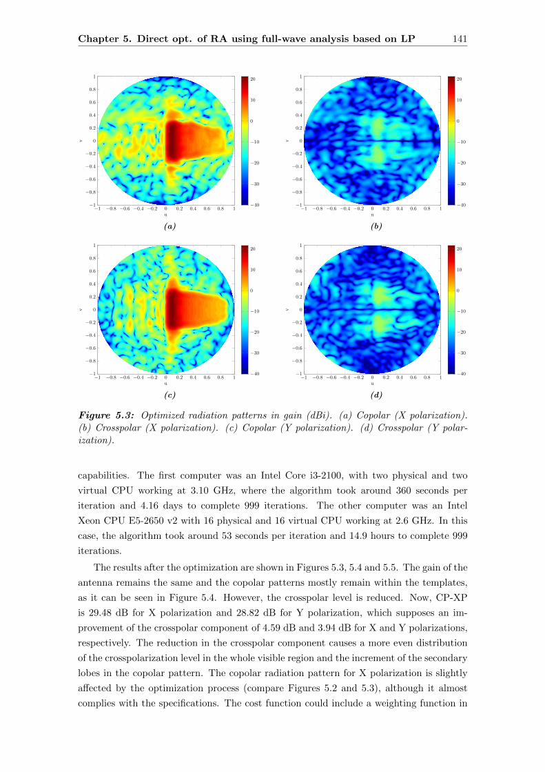
Chapter 5. Direct opt. of RA using full-wave analysis based on LP 141
−1 −0.8 −0.6 −0.4 −0.2 0 0.2 0.4 0.6 0.8 1−1
−0.8
−0.6
−0.4
−0.2
0
0.2
0.4
0.6
0.8
1
u
v
−40
−30
−20
−10
0
10
20
(a)
−1 −0.8 −0.6 −0.4 −0.2 0 0.2 0.4 0.6 0.8 1−1
−0.8
−0.6
−0.4
−0.2
0
0.2
0.4
0.6
0.8
1
u
v
−40
−30
−20
−10
0
10
20
(b)
−1 −0.8 −0.6 −0.4 −0.2 0 0.2 0.4 0.6 0.8 1−1
−0.8
−0.6
−0.4
−0.2
0
0.2
0.4
0.6
0.8
1
u
v
−40
−30
−20
−10
0
10
20
(c)
−1 −0.8 −0.6 −0.4 −0.2 0 0.2 0.4 0.6 0.8 1−1
−0.8
−0.6
−0.4
−0.2
0
0.2
0.4
0.6
0.8
1
u
v
−40
−30
−20
−10
0
10
20
(d)
Figure 5.3: Optimized radiation patterns in gain (dBi). (a) Copolar (X polarization).(b) Crosspolar (X polarization). (c) Copolar (Y polarization). (d) Crosspolar (Y polar-ization).
capabilities. The first computer was an Intel Core i3-2100, with two physical and two
virtual CPU working at 3.10 GHz, where the algorithm took around 360 seconds per
iteration and 4.16 days to complete 999 iterations. The other computer was an Intel
Xeon CPU E5-2650 v2 with 16 physical and 16 virtual CPU working at 2.6 GHz. In this
case, the algorithm took around 53 seconds per iteration and 14.9 hours to complete 999
iterations.
The results after the optimization are shown in Figures 5.3, 5.4 and 5.5. The gain of the
antenna remains the same and the copolar patterns mostly remain within the templates,
as it can be seen in Figure 5.4. However, the crosspolar level is reduced. Now, CP-XP
is 29.48 dB for X polarization and 28.82 dB for Y polarization, which supposes an im-
provement of the crosspolar component of 4.59 dB and 3.94 dB for X and Y polarizations,
respectively. The reduction in the crosspolar component causes a more even distribution
of the crosspolarization level in the whole visible region and the increment of the secondary
lobes in the copolar pattern. The copolar radiation pattern for X polarization is slightly
affected by the optimization process (compare Figures 5.2 and 5.3), although it almost
complies with the specifications. The cost function could include a weighting function in
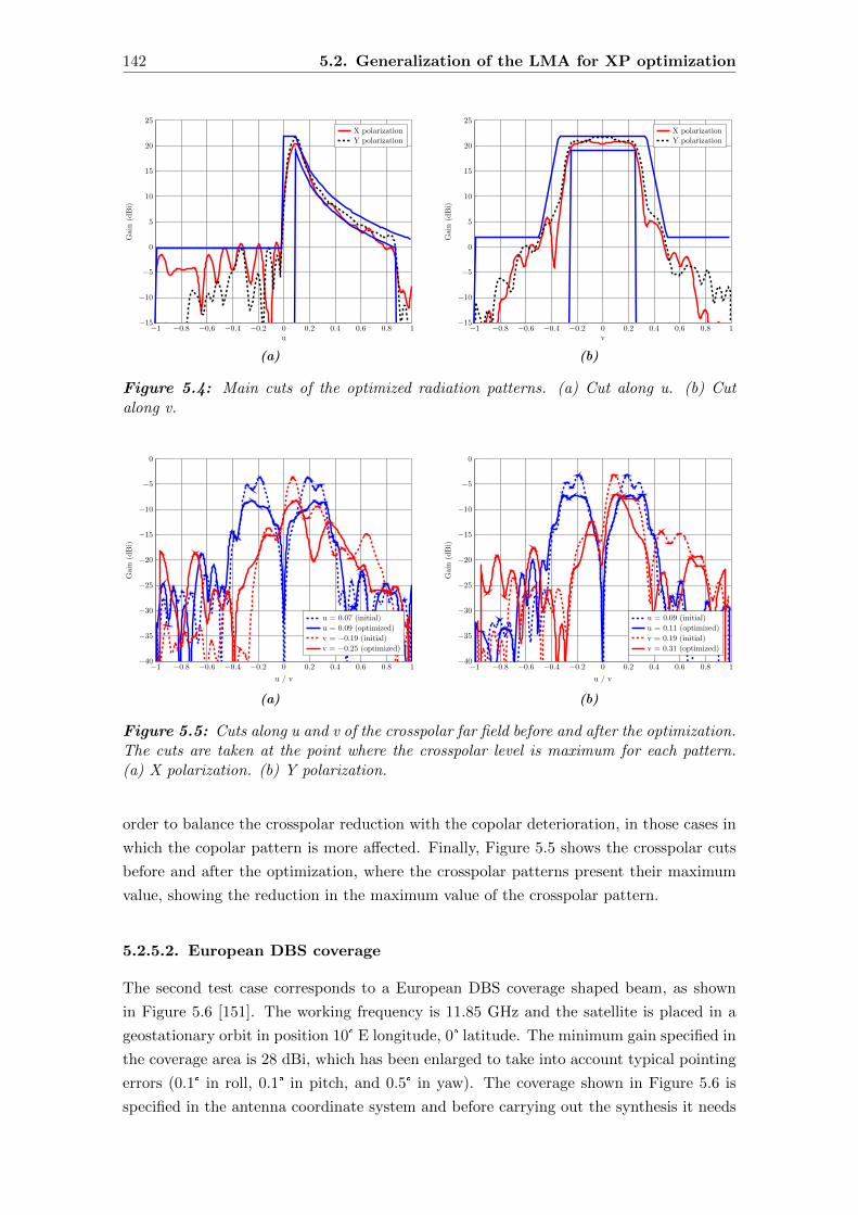
142 5.2. Generalization of the LMA for XP optimization
−1 −0.8 −0.6 −0.4 −0.2 0 0.2 0.4 0.6 0.8 1−15
−10
−5
0
5
10
15
20
25
u
Gain
(dBi)
X polarizationY polarization
(a)
−1 −0.8 −0.6 −0.4 −0.2 0 0.2 0.4 0.6 0.8 1−15
−10
−5
0
5
10
15
20
25
v
Gain
(dBi)
X polarizationY polarization
(b)
Figure 5.4: Main cuts of the optimized radiation patterns. (a) Cut along u. (b) Cutalong v.
−1 −0.8 −0.6 −0.4 −0.2 0 0.2 0.4 0.6 0.8 1−40
−35
−30
−25
−20
−15
−10
−5
0
u / v
Gain
(dBi)
u = 0.07 (initial)
u = 0.09 (optimized)
v = −0.19 (initial)
v = −0.25 (optimized)
(a)
−1 −0.8 −0.6 −0.4 −0.2 0 0.2 0.4 0.6 0.8 1−40
−35
−30
−25
−20
−15
−10
−5
0
u / v
Gain
(dBi)
u = 0.09 (initial)
u = 0.11 (optimized)
v = 0.19 (initial)
v = 0.31 (optimized)
(b)
Figure 5.5: Cuts along u and v of the crosspolar far field before and after the optimization.The cuts are taken at the point where the crosspolar level is maximum for each pattern.(a) X polarization. (b) Y polarization.
order to balance the crosspolar reduction with the copolar deterioration, in those cases in
which the copolar pattern is more affected. Finally, Figure 5.5 shows the crosspolar cuts
before and after the optimization, where the crosspolar patterns present their maximum
value, showing the reduction in the maximum value of the crosspolar pattern.
5.2.5.2. European DBS coverage
The second test case corresponds to a European DBS coverage shaped beam, as shown
in Figure 5.6 [151]. The working frequency is 11.85 GHz and the satellite is placed in a
geostationary orbit in position 10° E longitude, 0° latitude. The minimum gain specified in
the coverage area is 28 dBi, which has been enlarged to take into account typical pointing
errors (0.1° in roll, 0.1° in pitch, and 0.5° in yaw). The coverage shown in Figure 5.6 is
specified in the antenna coordinate system and before carrying out the synthesis it needs

Chapter 5. Direct opt. of RA using full-wave analysis based on LP 143
−u = − sin θ cosϕ
v=
sinθsinϕ
Figure 5.6: European coverage. (u, v) are in the antenna coordinate system.
−500 −400 −300 −200 −100 0 100 200 300 400 500
−400
−300
−200
−100
0
100
200
300
400
Coordinates of the elements in xr (mm)
Coordinates
oftheelem
ents
iny r
(mm)
−350
−300
−250
−200
−150
−100
−50
0
(a)
−500 −400 −300 −200 −100 0 100 200 300 400 500
−400
−300
−200
−100
0
100
200
300
400
Coordinates of the elements in xr (mm)
Coordinates
oftheelem
ents
iny r
(mm)
−350
−300
−250
−200
−150
−100
−50
0
(b)
Figure 5.7: Distribution phases for the design of the starting point for the reflectarraywith European DBS coverage. (a) Polarization X. (b) Polarization Y.
to be transformed to the reflectarray coordinate system defined in Figure 2.3 [2].
The reflectarray is square and formed by 5180 elements in a regular grid of 74 × 70
cells. The feed horn is modeled as a cosq θ function [78] with a q-factor of 23, which
provides an illumination taper of −17.9 dB at the reflectarray edges. The feed horn is
placed at ~rf = (358, 0, 1070) mm with regard to the reflectarray center. The period of
the unit cell is 14 mm × 14 mm, which is 0.55λ at the working frequency. Now, the
substrate for the lower layer has a height of 2.363 mm and a complex relative permittivity
εr = 2.55 − j2.295 · 10−3, while the upper layer has a height of 1.524 mm and a complex
relative permittivity εr = 2.17− j1.953 · 10−3.
For the starting point, a POS is carried out with the generalized Intersection Ap-
proach [89] starting with a properly focused reflectarray. After the POS, the phases
shown in Figure 5.7 were obtained. The layout of the reflectarray is obtained using the
unit cell shown in Figure 5.1 and a zero-finding routine, in such a way that the phases of
ρxx and ρyy match the required phase shift for each element as imposed by Figure 5.7 [2].
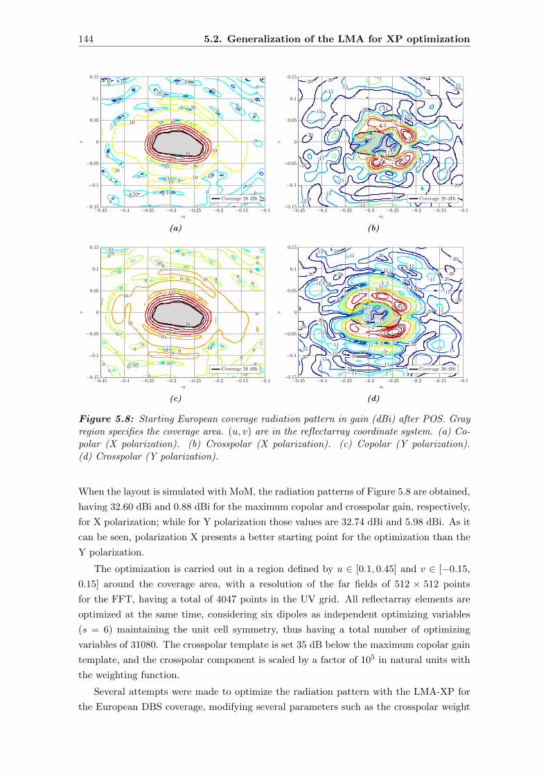
144 5.2. Generalization of the LMA for XP optimization
−0.45 −0.4 −0.35 −0.3 −0.25 −0.2 −0.15 −0.1−0.15
−0.1
−0.05
0
0.05
0.1
0.15-10
-10
-10
-10
-10
-10
-10
-10
-10
0
00
00
0
0
00
0
0
0
0
0
0
0
0
0
0
0
0 0
00
0
0
0
0 0
0
00
010
10
1010
10
10
10
10
20 25 2830
-u
v
Coverage 28 dBi
(a)
−0.45 −0.4 −0.35 −0.3 −0.25 −0.2 −0.15 −0.1−0.15
−0.1
−0.05
0
0.05
0.1
0.15
-20
-20 -20
-20
-20
-20
-20
-20
-20
-20
-20
-20
-20
-20-20
-20
-20-20
-20
-15
-15
-15
-15
-15
-15
-15
-15
-15
-15
-15
-15
-15
-15
-15
-15
-15
-11
-11
-11
-11
-7
-7
-5
-5-3
-3
-3
-3
-2
-2
-2
-u
v
Coverage 28 dBi
(b)
−0.45 −0.4 −0.35 −0.3 −0.25 −0.2 −0.15 −0.1−0.15
−0.1
−0.05
0
0.05
0.1
0.15-10-10
-10-10
-10
-10
-10
-10
0
0
0
0
0
0
0
0
0
0
0
0
00
0
0
0
0
0
0 0
0
0
0
0
0
0
0
0
0
10
10
10
10
10
10
20 25 2830
-u
v
Coverage 28 dBi
(c)
−0.45 −0.4 −0.35 −0.3 −0.25 −0.2 −0.15 −0.1−0.15
−0.1
−0.05
0
0.05
0.1
0.15
-20
-20
-20
-20
-20
-20
-20
-20
-20
-20
-20
-20
-20
-20
-20
-20
-20
-20
-20
-20
-20
-20
-20
-20
-15
-15
-15
-15 -15
-15
-15
-15
-15
-15
-15
-15
-15
-15
-15
-15
-11
-11
-11
-11
-11
-11
-11
-11
-11
-11
-11
-11
-11
-11
-11
-7
-7
-7-7
-7
-5
-5
-5
-5
-2
-2
2
2
2
2
3
3
3
4
45
-u
v
Coverage 28 dBi
(d)
Figure 5.8: Starting European coverage radiation pattern in gain (dBi) after POS. Grayregion specifies the coverage area. (u, v) are in the reflectarray coordinate system. (a) Co-polar (X polarization). (b) Crosspolar (X polarization). (c) Copolar (Y polarization).(d) Crosspolar (Y polarization).
When the layout is simulated with MoM, the radiation patterns of Figure 5.8 are obtained,
having 32.60 dBi and 0.88 dBi for the maximum copolar and crosspolar gain, respectively,
for X polarization; while for Y polarization those values are 32.74 dBi and 5.98 dBi. As it
can be seen, polarization X presents a better starting point for the optimization than the
Y polarization.
The optimization is carried out in a region defined by u ∈ [0.1, 0.45] and v ∈ [−0.15,
0.15] around the coverage area, with a resolution of the far fields of 512 × 512 points
for the FFT, having a total of 4047 points in the UV grid. All reflectarray elements are
optimized at the same time, considering six dipoles as independent optimizing variables
(s = 6) maintaining the unit cell symmetry, thus having a total number of optimizing
variables of 31080. The crosspolar template is set 35 dB below the maximum copolar gain
template, and the crosspolar component is scaled by a factor of 105 in natural units with
the weighting function.
Several attempts were made to optimize the radiation pattern with the LMA-XP for
the European DBS coverage, modifying several parameters such as the crosspolar weight

Chapter 5. Direct opt. of RA using full-wave analysis based on LP 145
−0.45 −0.4 −0.35 −0.3 −0.25 −0.2 −0.15 −0.1−0.15
−0.1
−0.05
0
0.05
0.1
0.15
-20
-20
-10-10
-10
-10
-10
-10
0
0 0
0
0
0
0
0
0
0
0
00
0
0
0
0
0
0
0
0
0
0
0
00
10
10
10
1010
10
10
10
10
10
10
10
10
10
10
10
10
10
202832
-u
v
Coverage 28 dBi
(a)
−0.45 −0.4 −0.35 −0.3 −0.25 −0.2 −0.15 −0.1−0.15
−0.1
−0.05
0
0.05
0.1
0.15
-20
-20-20
-20
-20
-20
-20
-20
-20
-20
-20
-20
-20
-20
-20
-20
-20-20-20
-20
-20
-20
-20
-20
-20
-20
-20
-15
-15
-15
-15
-15-15
-15
-15
-15
-15
-15
-15
-15
-15
-15
-15
-15
-15
-15
-15
-15
-15
-15
-15
-15
-11
-11
-11
-11
-11
-11
-11
-11
-11-11
-11
-11
-7
-7
-7
-7
-7
-7
-5
-5
-3
-3
-1
-1
-1
-u
v
Coverage 28 dBi
(b)
−0.45 −0.4 −0.35 −0.3 −0.25 −0.2 −0.15 −0.1−0.15
−0.1
−0.05
0
0.05
0.1
0.15
-10-10
-10
0
0
0
0
0
00
0
00
0
0
0
0
0
00
0
0 0
10
10
10
10
10
10
10
10
10
10
1010
10
10
10
10
202832
-u
v
Coverage 28 dBi
(c)
−0.45 −0.4 −0.35 −0.3 −0.25 −0.2 −0.15 −0.1−0.15
−0.1
−0.05
0
0.05
0.1
0.15
-20
-20-20
-20
-20
-20
-20
-20
-20-20
-20
-20-20
-20
-20
-20
-20
-20
-20
-20
-15
-15
-15
-15
-15
-15
-15
-15-15
-15
-15
-15
-15
-15
-15
-15
-15
-15
-15
-11
-11
-11
-11-11
-11
-11-11
-11
-11
-11
-11
-11
-11
-11
-11
-7
-7
-7
-7
-7
-5
-5
-5
-3
-3
-1
-1
2
2
3
3
-u
v
Coverage 28 dBi
(d)
Figure 5.9: European coverage radiation pattern in gain (dBi) after the optimization withthe LMA-XP. Gray region specifies the coverage area. (u, v) are in the reflectarray coordi-nate system. (a) Copolar (X polarization). (b) Crosspolar (X polarization). (c) Copolar(Y polarization). (d) Crosspolar (Y polarization).
in the cost function, allowing more ripple in the coverage zone and allowing higher side
lobes in the copolar pattern, without obtaining good results. In all instances the algorithm
converged to undesired local minima, obtaining similar and poor results. As an example,
Figure 5.9 shows the results when the crosspolar template was set 30 dB below the max-
imum copolar gain, the allowed ripple in the copolar pattern was 3 dB and the side lobe
levels were set 15 dB below the maximum copolar level, all set to facilitate convergence.
The crosspolar pattern was scaled by a factor of 104 in natural units. The results shown
belong to iteration 178 of the LMA-XP. (Original specifications for the optimization were:
crosspolar template 35 dB below the maximum copolar value, copolar ripple of 2 dB, side
lobe levels of −30 dB and scaling factor for the crosspolar component of 105 in natu-
ral units, for which the algorithm also diverged with similar results.) As it can be seen
comparing Figures 5.8 and 5.9, the crosspolar component for Y polarization reduced its
maximum value from 5.98 dB to 3.08 dB, although the crosspolar pattern for X polariza-
tion deteriorated, increasing its maximum original value of −0.88 dB to 1.27 dB, while
the coverage area was seriously affected for both polarizations, not fulfilling specifications

146 5.3. Generalization of the LMA for XP optimization
in most of the area.
It is important to note that, regardless of possible improvements in the crosspolar
levels, if the coverage area is affected as much as in this case, the obtained layout would
not be useful. In addition, the maximum crosspolar values were outside the coverage area
before the optimization, as it can be seen in Figure 5.8. However, after the optimization,
even though in the case of Y polarization this value is reduced, is now situated, for both
polarizations, inside the coverage area, which seriously penalizes the performance of the
antenna.
5.2.6. Conclusions and discussion
The Levenberg-Marquardt algorithm has been adapted to optimize the crosspolar compo-
nent of reflectarray antennas using MoM based on local periodicity in the computations.
Because the MoM routine is slow, the algorithm has been fully optimized in order to take
advantage of the resources available. In particular, all building blocks of the algorithm
have been conveniently parallelized and optimized in order to reduce the number of MoM
calls. An optimization has been carried out in two different computers in order to assess
the scalability of the proposed technique. An LMDS radiation pattern has been chosen as
a test case in which the crosspolar far field has been reduced 4.59 dB and 3.94 dB for the
X and Y polarizations, respectively, while mostly preserving the copolar pattern within
specifications.
Another example of a reflectarray with a European coverage for DBS applications was
tested. The reflectarray was comprised of 5180 elements and 31080 variables were opti-
mized. However, the algorithm converged to undesired local minima and poor results were
obtained. Several optimizations were tried to optimize this configuration, always obtain-
ing similar poor results. Despite the good results optimizing the crosspolar component of
a small-sized reflectarray, the algorithm does not provide good results when confronted to
larger reflectarrays due to the high number of variables involved. This happens due to local
minima which the LMA encounters during the optimization process. It could be partially
solved by employing a similar mechanism in the IA-POS, in which the number of degrees
of freedom was reduced by increasing the q-factor in the feed model. Here, the number of
optimizing variables could be reduced, resulting in a similar approach. Furthermore, by
reducing the number of optimizing variables not only the degrees of freedom are reduced,
hence reducing the amount of local minima; but also the computing times and memory
usage. However, as it was mentioned in the previous chapter when describing the LMA, it
performs a non-convex optimization due to the non-convexity of the lower bound used in
the cost function [152, 153]. This problem will limit the performance of the algorithm for
large reflectarrays, even when the strategy of reducing the number of optimizing variables
is employed.
A better strategy is proposed to overcome the limitations of the LMA-XP for large
reflectarrays, which consists in using another algorithm in order to improve the convergence
properties of the LMA. For that purpose, a generalized Intersection Approach algorithm
for the crosspolar optimization of reflectarrays with MoM based on local periodicity is

Chapter 5. Direct opt. of RA using full-wave analysis based on LP 147
described and compared with the LMA-XP detailed in this section.
5.3. The generalized Intersection Approach for direct
crosspolar optimization
In this section, the Intersection Approach framework is employed in a more generalized
approach [89] in order to improve the convergence for the crosspolar optimization of re-
flectarrays by working directly with MoM. Although the IA was extensively detailed in
a previous chapter, first for POS and later for the synthesis of Rmn matrices (IA-POS
and IA-XP, respectively), it will be briefly summarized again from the point of view of
improving its convergence properties.
5.3.1. Convergence improvement
The IA considers two sets, the set of the radiation patterns that can be obtained with the
reflectarray (set R) and the set of radiation patterns that comply with the specifications
(set M). At each iteration of the algorithm, the following operation is performed:
~Ei+1 = B[F(~Ei
)], (5.11)
where ~E is the radiated far field by the antenna. F is the forward projector which projects
the far field radiated by the antenna (belonging to the R set) onto the set of fields that
comply with the specifications (M set). Conversely, B is the backward projector which
projects the far field that fulfills the specifications onto the set of far fields that can be
radiated by the reflectarray. The goal of (5.11) is to find a radiation pattern that belongs
simultaneously to both sets, or if that is not possible, to find a radiation pattern whose
distance to the set of patterns that fulfill the requirements is minimal. Also, the IA is a
local optimizer and as such the starting point is of the utmost importance since it will
determine the correct converge of the algorithm [89].
The potential local minima reached by local optimizers are commonly known as traps.
In the IA framework, there are two main sources of traps [89]: the number of degrees
of freedom, which in this case will be the number of optimizing variables; and the non-
convexity of the involved sets. The latter problem can be addressed by working with the
squared field amplitude instead of the field itself. The gain is also suitable since it is
proportional to the squared field amplitude,
G ∝∣∣∣ ~E∣∣∣2 , (5.12)
and the specifications are usually given in gain. This improves the convergence of the
algorithm since it convexifies the set M of radiation patterns that comply with the spec-
ifications [89]. However, this leads to a redefinition of the backward projector in the
IA-POS and IA-XP since the FFT cannot be used anymore. It causes the algorithm to
lose the efficiency derived from the FFT being the most time consuming operation, and

148 5.3. The generalized IA for direct XP optimization
needing to use some optimization algorithm, which in the case of the present thesis is the
LMA.
For the first problem the solution is to reduce the number of variables in the first
steps of the synthesis process. This has been implemented in the IA-POS with a fictitious
reduction of variables modifying the illumination taper of the feed [95]. Nevertheless,
since the reflectarray geometry is optimized with the LMA, the variable reduction is not
fictitious anymore, since one can choose which variables will be optimized and which will
not.
In order to alleviate the notation, the compact notation for both polarizations will be
avoided and generic gains and templates will be used when possible, although keeping in
mind that the process is done for both polarizations and components of the far field.
5.3.2. Forward projection
The forward projector is divided in two steps, being the first one optional. In the first
step, the templates are normalized to the value of the gain of the far fields in a given
direction. Then, the fields are trimmed using those normalized templates, obtaining a
far field which complies with the specifications, but cannot, in general, be radiated by a
passive reflectarray.
The requirements of the copolar radiation pattern are usually given in gain, with a
maximum and minimum value. If these templates remain unaltered (i.e., the first step is
skipped), the synthesis is carried out in fixed gain. This method can be useful to further
refine a previous synthesis. Alternatively, they can be normalized to the gain in a given
(u0, v0) direction which belongs to the maximum gain region. It is then said that the
synthesis is carried out in float gain [95]. This method is more useful when a synthesis is
started from scratch (e.g. when doing POS) since it adapts automatically the templates to
the maximum gain that can be obtained with the reflectarray. In this case, a normalizing
constant is defined as
Cn =Gcp (u0, v0)
Tav, (5.13)
where Tav is the average value of the maximum and minimum copolar templates in the
(u0, v0) direction
Tav =Tcp,max(u0, v0) + Tcp,min(u0, v0)
2. (5.14)
Cn is defined for both polarizations independently to adapt the template to the current
gain of each polarization. Then, it is applied to both copolar and crosspolar templates as
Tncp(u, v) = Tcp(u, v) · Cn, (5.15a)
Tnxp(u, v) = Txp(u, v) · Cn. (5.15b)
The normalization in (5.15) is applied to the minimum and maximum templates of both
polarizations. This normalization process sets the middle point of the templates at (u0, v0)
at the same level of the gain in that direction.

Chapter 5. Direct opt. of RA using full-wave analysis based on LP 149
Once the templates have been normalized, both components of the radiated field should
accomplish the following condition in both polarizations
Tncp,min(u, v) ≤ Gcp(u, v) ≤ Tn
cp,max(u, v), (5.16a)
Tnxp,min(u, v) ≤ Gxp(u, v) ≤ Tn
xp,max(u, v). (5.16b)
This condition can be fulfilled by the Pr operator, defined for all (u, v) as follows for a
generic gain G,
Pr (G) =
Tnmax(u, v), Tn
max(u, v) < G(u, v)
Tnmin(u, v), Tn
min(u, v) > G(u, v)
G(u, v), otherwise,
(5.17)
The result of this operation is the gain G′,
G′(u, v) = Pr (G(u, v)) . (5.18)
For the sake of simplicity, a generic G gain component and normalized template Tn were
used in (5.17) and (5.18), but they should be applied to the copolar and crosspolar compo-
nents of both polarizations with their respective normalized templates. Also, the forward
projector only works with the gain (which is proportional to the squared field amplitude)
and the far field phase does not play any role, being able to take any value. In contrast
to the IA-POS and IA-XP, where the far field phase remained unchanged, now there is no
such constraint, improving the converge of the algorithm.
5.3.3. Backward projection
Since the forward projection works with the squared field amplitude (gain) instead of the
field itself, the FFT to recover the source field cannot be used. In any case, since the goal is
to directly optimize the geometry of the reflectarray to improve the crosspolar far field, an
optimization algorithm will be used. Now, the B operator is defined as the minimization
of the distance of an element m ∈ M to the set R,
dist (m,R) . (5.19)
For the minimization of the distance in (5.19), at this stage we have the element m as
the trimmed gain G′(u, v) of (5.18) and the current reflectarray geometry which generates
a gain pattern that belongs to the R set, G(u, v). As a distance definition, the Euclidean
norm for square-integrable functions can be used, which can be easily implemented by the
weighted Euclidean metric
d = dist2(G′(u, v), G(u, v)
)=
∫∫Ωw(u, v)
(G′(u, v)−G(u, v)
)2du dv, (5.20)
where w(u, v) is a weighting function and Ω is the area belonging to the visible region

150 5.3. The generalized IA for direct XP optimization
(u2+ v2 ≤ 1) where the far fields are optimized. This area can be the whole visible region
or located around the coverage zone. Since the radiated fields are already discretized in
the UV grid, the integral in (5.20) can be approximated by a sum for the UV points which
lie in Ω,
d =∑u,v
w(u, v)(G′(u, v)−G(u, v)
)2∆u∆v =
∑u,v
[C(u, v)
(G′(u, v)−G(u, v)
)]2, (5.21)
where
C(u, v) =√w(u, v)∆u∆v, (5.22)
and ∆u and ∆v are the steps in the discretized UV grid in u and v, respectively.
On the other hand, the LMA minimizes cost functions of the form [101]
F (x) =M∑i=1
(ri(x))2 , (5.23)
where r(x) is known as residual, which is discretized in M points. Comparing (5.21) with
(5.23) it is clear that
r(u, v) = C(u, v)(G′(u, v)−G(u, v)
), (5.24)
so the LMA naturally minimizes the distance between the two gain patterns.
The generic gains G and G′ need to accommodate the copolar and crosspolar compo-
nents for both polarizations. They can be implemented as vectors of size 4M × 1, where
M is the number of points in which each component of the gain is discretized. Also, since
the relative value of the crosspolar component is significantly lower than the copolar gain,
in order to properly reduce its starting value it might be convenient to scale the cross-
polar residual by means of the weighting function contained in C(u, v). Finally, it is not
necessary to attain a minimum (generally local) of (5.19), only to decrease the distance
at each iteration of the IA, so very few iterations of the LMA are needed.
The LMA described in the previous chapter is used here to directly optimize the re-
flectarray geometry. It also includes the optimizations described in this very same chapter
when it was used in a standalone version (known as LMA-XP) to directly optimize the
reflectarray geometry. The only change in the LMA is the definition of cost function,
which now is (5.21). The implemented new algorithm is now known as IA-LMA-XP and
is able to handle thousands of optimizing variables obtaining good results due to its im-
proved convergence properties derived from the use of the squared field amplitude and the
elimination of the far field phase constraint (which now can take any value), provided a
suitable starting point. Also, in order to control computing times and memory usage, the
number of optimizing variables can be reduced as well as the number of points in the UV
grid where the optimization is performed, carrying it out, for instance, only around the
coverage area instead of in the whole visible region.

Chapter 5. Direct opt. of RA using full-wave analysis based on LP 151
5.3.4. Validation
In order to validate the algorithm described in this section, two shaped patterns for satellite
applications are optimized in order to lower their crosspolar levels while maintaining the
copolar pattern within specifications. The patterns are an isoflux pattern for global Earth
coverage and a European coverage for DBS application [151]. In both cases, a POS is done
using the IA-POS [95] and then a design is obtained following [2], using the reflectarray
element of Figure 5.1. The unit cell is comprised of two layers of metallizations with four
parallel and coplanar dipoles for each polarization, and is described in detail in [43,127].
These two designs are used as starting point for the crosspolar optimization. The
copolar template is the same as the one used in the POS, and the crosspolar template is
defined as a certain constant value below the maximum copolar level, for the whole region
where the optimization is carried out.
5.3.4.1. Isoflux pattern
The first test case is an isoflux pattern for global Earth coverage. In Chapter 3 was detailed
how to obtain a parametrized isoflux pattern, which in this case has been particularized
for θ0 = 20°, a geostationary orbit, side lobe level 19 dB below the maximum copolar level
and 0.35 dB of allowable ripple in the coverage area.
The reflectarray is circular, with 1020 total elements placed in a rectangular grid with
36 elements along the diameter in both reflectarray axes. The feed horn is modeled as a
cosq θ function [78] with a q-factor of 14.8, which provides an illumination taper of −12 dB
at the reflectarray edges. The feed horn is placed at ~rf = (40, 0, 195) mm with regard to
the reflectarray center. The working frequency is 30 GHz and the period of the unit cell
is 5 mm × 5 mm (0.5λ). The substrate for both layers of the unit cell is the same, with
a height of 0.787 mm and a complex relative permittivity εr = 2.33 − j3.029 · 10−3. The
starting point for the crosspolar optimization is the POS carried out in Chapter 3, whose
phases are shown in Figure 3.8. A design using the cell of Figure 5.1 is done following [2],
which will be optimized.
The optimization is carried out in the whole visible region, with a resolution of the far
fields of 256× 256 points for the FFT, having a total of 51543 points in the UV grid and
using the First Principle of Equivalence. All of the reflectarray elements are optimized at
the same time, considering all dipoles as independent optimizing variables (s = 8), so the
total number of optimizing variables is 8160. The optimization is carried out in fixed gain,
setting the required gain to 18.35 dB in the center of the coverage zone. The crosspolar
template is set 35 dB below the maximum copolar gain template, and the crosspolar
component is scaled by a factor of 100 in natural units with the weighting function. The
LMA is set to perform three iterations per iteration of the IA.
The results obtained after the optimization are compared to the starting point in
Figures 5.10 and 5.11. On the one hand, Figure 5.10 shows the results for the copolar
pattern. There were two goals: to maintain the copolar specification (isoflux shape) while
reducing the crosspolar component, and to increase the gain for Y polarization while
maintaining the X polarization gain. As it can be seen, the starting point has around

152 5.3. The generalized IA for direct XP optimization
−1 −0.8 −0.6 −0.4 −0.2 0 0.2 0.4 0.6 0.8 1−10
−5
0
5
10
15
20
u
Gain(dBi)
X pol. (initial)
X pol. (optimized)
Y pol. (initial)
Y pol. (optimized)
0.1 0.15 0.2 0.25 0.3 0.35 0.4 0.45 0.5 0.55 0.6
17
18
19
(a)
−1 −0.8 −0.6 −0.4 −0.2 0 0.2 0.4 0.6 0.8 1−10
−5
0
5
10
15
20
vGain(dBi)
X pol. (initial)
X pol. (optimized)
Y pol. (initial)
Y pol. (optimized)
−0.25 −0.2 −0.15 −0.1 −0.05 0 0.05 0.1 0.15 0.2 0.25
17
18
19
(b)
Figure 5.10: Main cuts for the copolar pattern for both polarizations before and afterthe crosspolar optimization. The copolar gain for Y polarization is increased during theoptimization. (a) Cut along u for v = 0. (b) Cut along v for u = 0.34.
−1 −0.8 −0.6 −0.4 −0.2 0 0.2 0.4 0.6 0.8 1−50
−45
−40
−35
−30
−25
−20
−15
−10
−5
0
u / v
Gain
(dBi)
u = 0.40 (initial)
u = 0.56 (optimized)
v = 0.11 (initial)
v = −0.07 (optimized)
(a)
−1 −0.8 −0.6 −0.4 −0.2 0 0.2 0.4 0.6 0.8 1−50
−45
−40
−35
−30
−25
−20
−15
−10
−5
0
u / v
Gain
(dBi)
u = 0.41 (initial)
u = 0.36 (optimized)
v = 0.10 (initial)
v = 0.06 (optimized)
(b)
Figure 5.11: Cuts along u and v of the crosspolar far field before and after the opti-mization. The cuts are taken at the point where the crosspolar level is maximum for eachpattern. (a) X polarization. (b) Y polarization.
0.4 dB less in gain for Y polarization than the other in the coverage area. However, after
the optimization, the gains for both polarizations become similar while mostly preserving
the copolar shape within specifications.
On the other hand, Figure 5.11 shows some cuts in (u, v) of the crosspolar patterns.
The cuts correspond to the points were the crosspolar is maximum, for both polarizations,
even though they are not the same for the patterns before and after the optimization. For
the X polarization, the initial maximum crosspolar level is −4.81 dBi, and is reduced by
8.36 dB to −13.17 dBi after the optimization. For the Y polarization, initially there is

Chapter 5. Direct opt. of RA using full-wave analysis based on LP 153
a maximum level of −4.12 dBi for the crosspolar component and is reduced an amount
of 9.05 dB to −13.17 dBi. This important crosspolar reduction is achieved while keeping
the gain of the copolar pattern (and slightly increasing it in the case of Y polarization)
and its shape. The trade-off is a slight increase in the side lobes, as seen in Figure 5.10
and a redistribution of the lobes in the crosspolar component, which is now more uniform
towards higher levels in the whole UV grid.
5.3.4.2. European DBS coverage
The second test case corresponds to a European DBS coverage shaped beam, as shown
in Figure 5.12 [151]. The working frequency is 11.85 GHz and the satellite is placed in a
geostationary orbit in position 10° E longitude, 0° latitude. The minimum gain specified in
the coverage area is 28 dBi, which has been enlarged to take into account typical pointing
errors (0.1° in roll, 0.1° in pitch, and 0.5° in yaw). The coverage shown in Figure 5.12 is
specified in the antenna coordinate system and before carrying out the synthesis it needs
to be transformed to the reflectarray coordinate system defined in Figure 2.3 [2].
The reflectarray is square and formed by 5180 elements in a regular grid of 74 × 70
cells. The feed horn is modeled as a cosq θ function [78] with a q-factor of 23, which
provides an illumination taper of −17.9 dB at the reflectarray edges. The feed horn is
placed at ~rf = (358, 0, 1070) mm with regard to the reflectarray center. The period of
the unit cell is 14 mm × 14 mm, which is 0.55λ at the working frequency. Now, the
substrate for the lower layer has a height of 2.363 mm and a complex relative permittivity
εr = 2.55 − j2.295 · 10−3, while the upper layer has a height of 1.524 mm and a complex
relative permittivity εr = 2.17− j1.953 · 10−3.
The optimization is carried out in a region defined by u ∈ [0.1, 0.45] and v ∈ [−0.15,
0.15] around the coverage area, with a resolution of the far fields of 512×512 points for the
FFT, having a total of 4047 points in the UV grid. All reflectarray elements are optimized
at the same time, considering six dipoles as independent optimizing variables (s = 6)
maintaining the unit cell symmetry, thus having a total number of optimizing variables of
−u = − sin θ cosϕ
v=
sinθsinϕ
Figure 5.12: European coverage. (u, v) are in the antenna coordinate system.

154 5.3. The generalized IA for direct XP optimization
−0.45 −0.4 −0.35 −0.3 −0.25 −0.2 −0.15 −0.1−0.15
−0.1
−0.05
0
0.05
0.1
0.15-10
-10
-10
-10
-10
-10
-10
-10
-10
0
00
00
0
0
00
0
0
0
0
0
0
0
0
0
0
0
0 0
00
0
0
0
0 0
0
00
010
10
1010
10
10
10
10
20 25 2830
-u
v
Coverage 28 dBi
(a)
−0.45 −0.4 −0.35 −0.3 −0.25 −0.2 −0.15 −0.1−0.15
−0.1
−0.05
0
0.05
0.1
0.15
-20
-20 -20
-20
-20
-20
-20
-20
-20
-20
-20
-20
-20
-20-20
-20
-20-20
-20
-15
-15
-15
-15
-15
-15
-15
-15
-15
-15
-15
-15
-15
-15
-15
-15
-15
-11
-11
-11
-11
-7
-7
-5
-5-3
-3
-3
-3
-2
-2
-2
-u
v
Coverage 28 dBi
(b)
−0.45 −0.4 −0.35 −0.3 −0.25 −0.2 −0.15 −0.1−0.15
−0.1
−0.05
0
0.05
0.1
0.15-10-10
-10-10
-10
-10
-10
-10
0
0
0
0
0
0
0
0
0
0
0
0
00
0
0
0
0
0
0 0
0
0
0
0
0
0
0
0
0
10
10
10
10
10
10
20 25 2830
-u
v
Coverage 28 dBi
(c)
−0.45 −0.4 −0.35 −0.3 −0.25 −0.2 −0.15 −0.1−0.15
−0.1
−0.05
0
0.05
0.1
0.15
-20
-20
-20
-20
-20
-20
-20
-20
-20
-20
-20
-20
-20
-20
-20
-20
-20
-20
-20
-20
-20
-20
-20
-20
-15
-15
-15
-15 -15
-15
-15
-15
-15
-15
-15
-15
-15
-15
-15
-15
-11
-11
-11
-11
-11
-11
-11
-11
-11
-11
-11
-11
-11
-11
-11
-7
-7
-7-7
-7
-5
-5
-5
-5
-2
-2
2
2
2
2
3
3
3
4
45
-u
v
Coverage 28 dBi
(d)
Figure 5.13: Starting European coverage radiation pattern in gain (dBi) after POS. Grayregion specifies the coverage area. (u, v) are in the reflectarray coordinate system. (a) Co-polar (X polarization). (b) Crosspolar (X polarization). (c) Copolar (Y polarization).(d) Crosspolar (Y polarization).
31080. The optimization is carried out in fixed gain, setting the required gain to 31.90 dB
in the direction (u0, v0) = (0.28, 0), allowing a ripple of 2 dB. The crosspolar template
is set 35 dB below the maximum copolar gain template, and the crosspolar component is
scaled by a factor of 105 in natural units with the weighting function. The LMA is set to
perform three iterations per iteration of the IA.
The starting point is the same as the one used in the LMA-XP optimization, where
the obtained phases after the POS are shown in Figure 5.7. After the layout was obtained
using the unit cell of Figure 5.1, the simulated radiation patterns with MoM are shown
again in Figure 5.13 for both linear polarizations. The gain requirements are fulfilled in
the whole extended coverage region (see Figure 5.12), having a maximum copolar gain
of 32.60 dBi and maximum crosspolar gain of −0.88 dBi for X polarization, while for
Y polarization those values are 32.74 dBi and 5.98 dBi for the maximum copolar and
crosspolar gain, respectively. As it can be seen, the starting point for Y polarization is
much worse than for X polarization, since the crosspolar pattern has a maximum value
almost 7 dB higher.

Chapter 5. Direct opt. of RA using full-wave analysis based on LP 155
−0.45 −0.4 −0.35 −0.3 −0.25 −0.2 −0.15 −0.1−0.15
−0.1
−0.05
0
0.05
0.1
0.15
-10-10
-10
-10-10
000
0
0
0
0
0
0
0
0
0
0
0
0
0
00
0
0
10
10
10
10
10
10
10
10
10
1010
10
10
10
10
20 25 2830
-u
v
Coverage 28 dBi
(a)
−0.45 −0.4 −0.35 −0.3 −0.25 −0.2 −0.15 −0.1−0.15
−0.1
−0.05
0
0.05
0.1
0.15
-20
-20
-20
-20
-20
-20
-20
-20
-20
-20
-20
-20
-20
-20
-20
-20
-20
-20
-20
-20
-20
-15
-15
-15
-15
-15
-15
-15
-15
-15
-15
-15
-15
-15
-15
-15
-15
-15
-11
-11
-11
-11
-11
-7
-7
-7
-5
-5
-5
-3
-u
v
Coverage 28 dBi
(b)
−0.45 −0.4 −0.35 −0.3 −0.25 −0.2 −0.15 −0.1−0.15
−0.1
−0.05
0
0.05
0.1
0.15
-10
-10
0
0
00
0
0
0
0
0
0
0
0
0
0
0
0
0
0
0
0
0
0
0
0
0
0
0
00
10
10
10
10
10
10
10
10
1010
20 25 2830
-u
v
Coverage 28 dBi
(c)
−0.45 −0.4 −0.35 −0.3 −0.25 −0.2 −0.15 −0.1−0.15
−0.1
−0.05
0
0.05
0.1
0.15
-20
-20
-20-20
-20
-20
-20
-20
-20
-20
-20
-20
-20
-20
-20
-20
-20
-20
-20
-20
-20
-20
-20
-20
-20
-20
-15
-15
-15
-15
-15
-15
-15
-15
-15
-15
-15
-15
-15
-15
-11
-11
-11
-11
-11
-11
-11
-11
-11
-11
-7-7
-7-7
-7
-7
-5
-5-5
-5
-3
-3
-u
v
Coverage 28 dBi
(d)
Figure 5.14: Optimized European coverage radiation pattern in gain (dBi) with the IA-LMA-XP. Gray region specifies the coverage area. (u, v) are in the reflectarray coordinatesystem. (a) Copolar (X polarization). (b) Crosspolar (X polarization). (c) Copolar (Ypolarization). (d) Crosspolar (Y polarization).
Figure 5.14 shows the optimized radiation pattern for both polarizations. For X po-
larization, the coverage zone is barely affected, and presents a maximum copolar gain of
32.13 dBi and a maximum crosspolar gain of −2.20 dBi (reduced an amount of 1.32 dB).
In the case of the Y polarization, the maximum copolar gain is 31.47 dBi while the maxi-
mum crosspolar gain is −2.20 dBi. Paying attention to the 30 dB contour, the pattern is
slightly worsen, but the specifications comply for a gain of 28 dBi in the whole coverage
region, while the maximum crosspolar gain has been substantially reduced (an amount of
8.18 dB).
A better parameter to analyze the crosspolar component of the radiation pattern is the
crosspolar discrimination (XPD), which is defined, for the coverage area, as the difference,
point by point, of the copolar and crosspolar components in dBi. Figure 5.15 shows the
XPD before and after the optimization for both polarizations. Due to the initial low
value for the crosspolar component, the XPDmin for X polarization is 33.46 dB, and it
barely improves after the optimization, obtaining a value of 33.94 dB (0.48 dB higher).
However, for Y polarization, the initial value of XPDmin was 25 dB and it improved to

156 5.3. The generalized IA for direct XP optimization
−0.34 −0.3 −0.26 −0.22−0.04
−0.03
−0.02
−0.01
0
0.01
0.02
0.03
-u
v
25
30
35
40
45
50
(a)
−0.34 −0.3 −0.26 −0.22−0.04
−0.03
−0.02
−0.01
0
0.01
0.02
0.03
-u
v
25
30
35
40
45
50
(b)
−0.34 −0.3 −0.26 −0.22−0.04
−0.03
−0.02
−0.01
0
0.01
0.02
0.03
-u
v
25
30
35
40
45
50
(c)
−0.34 −0.3 −0.26 −0.22−0.04
−0.03
−0.02
−0.01
0
0.01
0.02
0.03
-uv
25
30
35
40
45
50
(d)
Figure 5.15: XPD before and after the optimization for the European coverage shapedbeam. (a) Pol. X before (XPDmin = 33.46 dB). (b) Pol. Y before (XPDmin = 25.00 dB).(c) Pol. X after (XPDmin = 33.94 dB). (d) Pol. Y after (XPDmin = 30.76 dB).
30.76 dB after the optimization (5.76 dB higher), despite defining the crosspolar template
as a constant value in a bigger region than the coverage zone and not directly optimizing
the XPD parameter.
Another parameter, stricter than XPD, is the crosspolar isolation (XPI), which is
defined, for the coverage area, as the difference between the minimum copolar gain and the
maximum crosspolar gain, both in dBi. For the case at hand, the initial XPI is 32.06 dB
and 23.88 dB for X and Y polarizations, respectively. After the optimization, the new
values for XPI are 32.62 dB (improvement of 0.56 dB) and 29.73 dB (improvement of
5.85 dB), for X and Y polarizations, respectively. As it happened to the XPD parameter,
the XPI is greatly improved for Y polarization, but not for X polarization, since the
starting point was already good.
5.3.5. Convergence improvement over the LMA-XP
The main goal of switching from the LMA-XP to the IA-LMA-XP was to improve the
convergence of the algorithm, to obtain better results in less iterations and to be able
to handle larger problems with success. The two examples shown to validate the IA-
LMA-XP proof the latter assertion. In order to compare both algorithms, a number of
optimizations were carried out for a LMDS pattern for different UV grid points and the
same number of optimizing variables. While the LMA-XP was only tried once for a UV
grid of 128 × 128, the IA-LMA-XP was tried for larger grids. The antenna specifications
and starting point for the optimization are the same as the ones described in Section
5.2.5.1 for the optimization of the LMDS pattern with the LMA-XP.

Chapter 5. Direct opt. of RA using full-wave analysis based on LP 157
Table 5.1: Comparison between the LMA-XP and IA-LMA-XP algorithms for the cross-polar optimization of a reflectarray antenna with LMDS pattern using a full-wave analysisbased on local periodicity.
UV grid # it CPx (dB) XPx (dB) CPy (dB) XPy (dB)
128× 128 1 20.52 −3.44 21.15 −2.94
256× 256 1 20.52 −3.41 21.17 −2.89
512× 512 1 20.54 −3.41 21.17 −2.89
1024× 1024 1 20.54 −3.40 21.17 −2.89
LMA-XP 128 659 20.42 −8.44 20.81 −6.99
IA-LMA-XP 128 177 20.78 −10.59 21.06 −9.82
IA-LMA-XP 256 219 20.76 −10.82 21.04 −10.59
IA-LMA-XP 512 120 20.83 −9.82 21.06 −8.89
IA-LMA-XP 1024 69 20.66 −7.05 21.00 −5.71
Table 5.1 shows the comparison between the two algorithms. The column with the
number of iterations correspond to the LMA iterations in the IA-LMA-XP, which was set
to perform three iterations per iteration of the IA. This column represents the iteration
at which the algorithm was stopped. The values of the copolar and crosspolar patterns
for both polarizations represent the maximum value in the whole visible region. As it can
be seen, the IA-LMA-XP provides better results in less iterations than the LMA-XP, due
to the improved convergence properties. For the heavier optimizations of the IA-LMA-
XP, with UV grids of 512 × 512 and 1024 × 1024 points, the optimizations were stopped
earlier due to the large amounts of time that they were taking. However, for the 512×512
grid the results were already better than those of the LMA-XP, and for the biggest grid,
although they still did not reach those of the LMA-XP, they were quite close with a tenth
of the iterations performed. If the last optimization would have been left more iterations,
it would improve the results of the LMA-XP.
5.4. Conclusions
In this chapter, the crosspolar optimization of reflectarray antennas by directly optimizing
the reflectarray element geometry has been addressed. First, the LMA was used, taking
advantage of all the improvements introduced in the previous chapter, along with some
new to minimize the impact of MoM in the optimization process. The algorithm, known
as LMA-XP, was tested with a LMDS pattern, obtaining good results in the crosspolar
optimization. However, since the cost function represents a non-convex search space, it
presents convergence problems for larger reflectarrays, since the number of local minima
grows exponentially with the number of optimizing variables. This was confirmed trying
to optimize a large reflectarray comprised of 5180 elements, optimizing more than 30000
variables at the same time. The algorithm always converged to non-desired local minima,
obtaining very poor results.
In order to address the convergence issue, it was decided to use a generalization of

158 5.4. Conclusions
the IA, working with the squared field amplitude, which convexifies the set of radiation
patterns that comply with the specifications. Although it does not convexify the whole
problem, it certainly alleviates the trap issue, as it was demonstrated with the two test
cases which are provided. Due to the improved convergence, the algorithm is able to handle
thousands of optimizing variables and still obtain good results in crosspolar optimization.
An isoflux pattern for global Earth coverage and a European coverage for DBS application
were optimized in order to validate the developed algorithm. In both cases good results
were obtained, and in the DBS coverage, the crosspolar component was reduced several dB
optimizing more than 30 thousand variables, while maintaining the copolar shape within
specifications.
The LMA-XP and IA-LMA-XP were compared to assess the improved convergence
achieved by the IA-LMA-XP. It was shown that not only is the IA-LMA-XP capable of
handling large problems (as demonstrated with the optimization of the large reflectarray
for DBS applications), but it also provides better results in less iterations than the LMA-
XP, which makes it a more suitable algorithm for the crosspolar optimization of reflectarray
antennas.

CHAPTER 6
Conclusions and future research
lines
6.1. Final conclusions
This thesis has been devoted to the development of efficient and accurate techniques for
the analysis and synthesis of reflectarray antennas for both far field and near field applica-
tions. With regard to the improvement of the analysis techniques, the efficient approach
to the far field computation of reflectarray antennas is based on the use of the Fast Fourier
Transform (FFT) algorithm, since it is able to compute the spectrum functions faster than
a direct implementation of the equations. Also, the accuracy was improved by consider-
ing each element of the reflectarray a small rectangular aperture, instead of a punctual
isotropic source. However, this analysis was only available for periodic reflectarrays in
the literature. When aperiodic reflectarrays were considered, there were two options. An
accurate analysis considering small apertures as the elements meant a slow computation of
the spectrum functions, since there was no efficient technique for their computation. For
an efficient analysis using the Non-Uniform FFT (NUFFT), the elements were considered
to be punctual isotropic sources, loosing accuracy. For the first time, a new formulation
has been developed that allows to efficiently compute the spectrum functions (and thus
the far fields) of aperiodic reflectarrays employing the NUFFT algorithm and modeling
each reflectarray element as small rectangular apertures. Furthermore, since the NUFFT
is a generalization of the FFT algorithm, it can also be applied to the periodic case over-
coming one limitation of the FFT use, that is, the impossibility of efficiently computing
the far fields in the whole visible region when the periodicity of the reflectarray is larger
than half a wavelength.
The reflectarray analysis also assumes a constant incident field on the surface of each
element (modeled as a small aperture). This assumption is convenient because it facili-
tates the analytical operations with the equations. In this thesis, a generalization of this
approach has been proposed, considering a continuous incident field on each cell. In the
new formulation, the field at each cell is considered to be narrowband since its variation is
159

160 6.1. Final conclusions
smooth in a period of the reflectarray. Thus, it is possible to represent such incident field
by means of its Fourier coefficients. Then, following a similar development as when the
incident field was constant, the spectrum functions could be computed as a linear combi-
nation of FFT for the periodic case, or a linear combination of NUFFT in the aperiodic
case. This new analysis technique could improve the characterization of secondary lobes
and crosspolar component of the radiated far fields.
When computing the far fields radiated by aperture antennas, three Principles of
Equivalence can be used, depending on the knowledge of the field in the aperture. Un-
til recently, it was common to employ the Second Principle of Equivalence, since it only
requires knowledge of the tangential electric field. However, the First Principle of Equiv-
alence provides more accurate results in both the copolar and crosspolar components. It
requires the tangential magnetic field in the aperture, which can be easily obtained by
assuming a locally incident plane wave at each reflectarray element. Furthermore, re-
flectarrays usually present a dielectric frame to screw the breadboard to the supporting
structures. It has been demonstrated the importance of correctly modeling such dielectric
frame in the design process since it can alter the radiation patterns, leading to a wrong
characterization of the far fields.
Although the new developments in far field analysis techniques previously described
were mainly focused for reflectarray antennas, they can be easily employed in the anal-
ysis of other planar-like structures, such as array antennas, transmitarrays or Frequency
Selective Surfaces (FSS), due to their similarities to reflectarray antennas.
A new model for the near field analysis of reflectarray antennas has been presented.
Again, instead of considering each element as a punctual source, it is modeled as a small
aperture. Then, the near field of the reflectarray antenna is computed at each point of
space as far field contributions of all the elements that comprise the array. The aim of this
analysis was the prediction of the quiet zone generated by reflectarrays. Hence, a detailed
development to compute the near field in planes perpendicular to the reflectarray pointing
direction was presented. The computation of the near field is slower than the far field,
since the FFT cannot longer be used. Thus, a strategy to parallelize its computation is
presented, speeding up computations taking advantage of modern computers. The near
field model presented in this thesis was validated by means of simulations with commercial
software as well as measurements.
The rest of the thesis is devoted to the development of efficient synthesis and opti-
mization techniques to improve the crosspolar component of the reflectarray far fields. In
addition, some of the developed algorithms were applied to the near field optimization in
order to improve the quiet zone generated by reflectarray antennas, with the future goal
of using reflectarrays as probes for Compact Antenna Test Ranges (CATR).
First, an efficient implementation of the Intersection Approach (IA) algorithm for
Phase-Only Synthesis (POS), and denoted IA-POS, was described. This algorithm has
been extensively used in the past for reflectarray synthesis with great success. The POS
formulation for the First Principle of Equivalence has been introduced for the first time.
Also, the algorithm has been improved by including the dielectric frame in the analysis

Chapter 6. Conclusions and future research lines 161
as well as a constraint in the backward projector to recover the field at the aperture. It
is a very efficient algorithm which can deal with very large reflectarrays. Its efficiency is
based on the use of the FFT to compute the far fields and to recover the source field.
Large reflectarrays are dealt with by modifying the illumination taper of the feed and
performing the synthesis in several steps, in order to reduce in the first steps the number
of local minima, minimizing the problem of traps and improving the algorithm conver-
gence. However, as a POS algorithm, it only deals with the copolar pattern, and there
is no control over the crosspolar one during the synthesis process. This fact motivated
the search for an efficient algorithm to synthesize/optimize the crosspolar component of
reflectarray antennas. Using the IA-POS as starting point, its formulation was extended
to include crosspolar requirements in the synthesis process, obtaining what is called the
IA-XP. In order to do that, instead of working with phase distributions, now the algorithm
works with reflection coefficient matrix distributions, since this matrix fully describes the
behavior of the element and can accurately account for the crosspolarization contribu-
tion of the reflectarray elements to the crosspolar pattern. As the IA-POS, the IA-XP
is computationally very efficient, since it still uses the FFT in both projectors, although
now four FFT are used in each projector instead of two in the IA-POS. Also, the IA-XP
does not perform any electromagnetic analysis of the periodic cell. If the IA-XP is left to
run without any constraints imposed to the reflection coefficient matrices, it will converge
quickly to the desired solution, although the coefficients will not be feasible for passive
reflectarrays since they will not meet the power balance. Hence, a complete formulation
was developed in order to obtain the feasibility conditions of lossy two-port networks in
order to implement those constraints in the algorithm. This way, the convergence is more
difficult, but the obtained reflection coefficients will be feasible for passive networks, in-
cluding passive reflectarrays. The algorithm was validated with a number of examples,
showing good results.
Despite developing an efficient algorithm along with suitable constraints to obtain fea-
sible passive reflection coefficients, it presents a major handicap. This is better understood
comparing it with the IA-POS. The output of the IA-POS is two phase distributions, one
for each polarization. The reflectarray design is obtained by adjusting the geometry of
each element to match the required phase. This is easy to achieve due to the good behavior
of the phases (almost linear in the desired variation range), because there are only two
parameters to adjust per reflectarray element, and it is easy to do since the orthogonal
dimensions of the element can almost adjust independently each required phase. However,
for the IA-XP case, instead of two real parameters to adjust with the geometry, there are
four complex numbers (equivalent to eight real parameters). Not only that, the reflection
crosscoeffients are highly non-linear, so finding a reflectarray layout that is able to match
the required reflection coefficient matrices is a really challenging task which was not pur-
sued in this work, although some guidelines were provided. Hence, a difference approach
was followed to be able to control the crosspolar component in the synthesis process.
The new approach was to directly optimize the geometry of the reflectarray elements
using a full-wave analysis tool based on local periodicity, Method of Moments (MoM)

162 6.1. Final conclusions
in this case. Due to this new layer added to the reflectarray analysis in the synthesis
process, the IA could no longer be used as implemented in the IA-POS and IA-XP. Now,
a general optimizing algorithm is needed. The Levenberg-Marquardt algorithm (LMA) was
chosen due to its simplicity and capacity to work with non-linear optimization problems.
However, instead of addressing directly the crosspolar optimization with the LMA, a POS
version was developed in order to study the algorithm and introduce several computing
optimizations to make the algorithm as fast as possible. This implementation is known as
LMA-POS. The improvements introduced in the algorithm were the parallelization of the
Jacobian matrix evaluation; minimization of the evaluation error of the derivatives which
are evaluated by finite difference; appropriate choice of the libraries to perform matrix-
vector and matrix multiplications; simplification of the matrix multiplication computing
only half the matrix, since the result is symmetric; and optimum choice of the matrix
equation solver, based on a Cholesky factorization due to the symmetric nature of the
problem. With these improvements, the LMA is greatly sped up. Furthermore, the
obtained results improve others in the literature. The implemented algorithm is accurate
and scalable.
Then, the LMA-POS was extended to include MoM as analysis tool in order to op-
timize the crosspolar radiation pattern, obtaining the LMA-XP algorithm. Despite the
improvements introduced in the LMA in the previous implementation, the inclusion of
MoM in the optimization caused the algorithm to be extremely slow and of no practical
use. Then, some strategies to minimize the impact of MoM were devised and implemented.
First, with regard to the finite differences, a lateral difference was employed, reducing by
half the calls to MoM. Also, for the computation of each column of the Jacobian, only one
element is modified. Hence, there is no need to recompute the tangential field processing
all elements with MoM, but just one, reusing the tangential field matrix from the first call
to the cost function at the beginning of each iteration of the LMA. Since a good starting
point is very important in a local optimizer, to test the LMA-XP, first a POS was carried
out for a LMDS pattern, and after the reflectarray design was obtained, the crosspolar
pattern was reduced several dB with the LMA-XP, verifying the proposed method. How-
ever, the LMA-XP presented some convergence issues when dealing with large reflectarrays
due to the increasing number of variables and that the LMA cost function represented a
non-convex search space. For that reason, it was necessary to improve the convergence of
the algorithm following a different path.
In order to improve the convergence of the LMA-XP, it was decided to employ the
generalized IA framework, which provided a more powerful and general framework to
deal with the synthesis problem. In particular, working with the squared field amplitude
instead of the field itself would alleviate the problem of local minima or traps. However,
this caused a redefinition of the backward projector, which now implied the minimization
of a distance, which needed to be implemented with an optimization algorithm. To take
advantage of all the previous work, the LMA was chosen as backward projector, with all
of its previous improvements. The resulting algorithm was denoted as IA-LMA-XP. The
new algorithm greatly improved the converge of the LMA-XP. Now, the IA-LMA-XP can

Chapter 6. Conclusions and future research lines 163
handle thousands of optimizing variables and still achieve good results. Two examples
were provided to validate the algorithm, one isoflux pattern for global Earth coverage,
and a European coverage for DBS applications. In both cases the crosspolar pattern was
greatly reduced while preserving the copolar shape, and in the latter case (DBS coverage),
there were more than 30 thousand optimizing variables. Still, computing times using MoM
in the optimization process were acceptable using a workstation. Also, the LMA-XP and
the IA-LMA-XP were compared in order to assess the convergence improvement, showing
that better results were obtained with the IA-LMA-XP in less iterations.
6.2. Original contributions
The original contributions of this thesis can be grouped depending on whether they are
aimed to far field or near field applications.
6.2.1. Contributions related to reflectarray analysis for far field
applications
Development of an efficient technique for the far field computation of aperiodic arrays
based on the Non-Uniform Fast Fourier Transform (NUFFT). The novelty of this
approach is that it considers each reflectarray element as a small aperture instead of a
punctual source (as in the array factor), increasing the accuracy of the computations.
Before this technique was available, the computations of radiated fields of aperiodic
reflectarrays only could be computed efficiently by using the NUFFT and the array
factor (loosing efficiency), or by a direct implementation of the double summations
of the spectrum functions, which is not efficient. Related papers: [J1, C4]. Related
projects: [P2].
Generalization of the reflectarray analysis considering a continuous incident field.
The incident field at each reflectarray element is represented by means of its Fourier
coefficients. Then, the spectrum functions are efficiently computed as a linear com-
bination of FFT or NUFFT, for periodic or aperiodic reflectarrays, respectively.
Related papers: [C4]. Related projects: [P3, P4, P5].
6.2.2. Reflectarray synthesis for far field applications
Design, manufacture, and measurement of a low-cost reflectarray for global Earth
coverage. The synthesis and design processes were conveniently adapted in order to
obtain a suitable reflectarray geometry based on a single rectangular patch backed by
a ground plane. Since this reflectarray element is not able to provide a full 360° phase-
shift, the IA-POS was modified in order to impose this phase constrain. Moreover,
since the behavior of the unit cell with regard to the patch size is non-linear, the
patch dimensions were constrained during the design process in order to ensure a
smooth distribution of the patches. This way, the local periodicity assumption of the
MoM tool is preserved and the obtained reflectarray design is more reliable. Finally,

164 6.2. Original contributions
simulations and measurements are in good agreement. Related papers: [J4]. Related
projects: [P3, P4, P5].
Improvement of the phase-only synthesis algorithms by developing a POS formu-
lation of the First Principle of Equivalence to correctly characterize the copolar
component of the far field. Related projects: [P3, P4, P5].
Improvement of the synthesis algorithms by including the effect of the dielectric
frame in the synthesis process as a constraint, since the field in the frame is not
modified during the synthesis process due to the lack of metallizations in that region
of the antenna. Related projects: [P3, P4, P5].
Efficient generalization of the Intersection Approach (IA) algorithm applied to dual-
linear planar reflectarray antennas including crosspolar requirements during the syn-
thesis process. Previously, the only efficient implementation of the IA algorithm only
allowed to perform phase-only synthesis (POS), which only deals with copolar re-
quirements during the synthesis process. The efficiency of the method lies in the use
of the FFT in both projectors, to compute the radiated far fields and to recover the
source field. The output of this new formulation of the IA is a distribution of re-
flection coefficient matrices, which fully characterize the behavior of the reflectarray
element. Related papers: [J2]. Related projects: [P3, P4, P5].
As part of the generalization of the IA algorithm described in the previous point, the
feasibility conditions for lossy passive networks were derived from the generalized
S matrix which characterize these networks. This development was carried out
modeling the reflectarray unit cell as a 2-port network in order to find appropriate
feasibility constraints to include during the synthesis process. Related papers: [J2].
Related projects: [P3, P4, P5].
Improvement of the Levenberg-Marquardt algorithm (LMA) for the POS of reflect-
array antennas, keeping in mind that it will be used later for the direct optimization
of the reflectarray geometry. All the building blocks of the algorithm have been
conveniently optimized in order to obtain a scalable algorithm. In particular, the
reflectarray analysis is efficient since it uses the FFT; the Jacobian matrix evaluation
is parallelized, computing one column per available thread; the matrix-vector and
matrix multiplications are performed by highly optimized and fully parallelized com-
mercial libraries which have been manually implemented using low-level hardware
instructions; and the matrix equation system is efficiently solved by a Cholesky-
based solver, which is the fastest solver available for this type of problem. The
implementation of the LMA in this thesis outperforms others reported in the liter-
ature, allowing to solver larger problems in less time. Related papers: [J3]. Related
projects: [P1].
Extension of the LMA to directly optimize the reflectarray geometry using a full-
wave Method of Moments based on local periodicity as analysis tool during the

Chapter 6. Conclusions and future research lines 165
optimization process. This way, the crosspolar component can be properly lowered
since the crosspolarization introduced by the elements is taken into account. All the
optimizations introduced for the POS version are used in this extension, and some
new are introduced in order to minimize the impact of MoM in the optimization. The
resulting algorithm was tested in a LMDS pattern for the crosspolar optimization,
lowering the crosspolar pattern several dB while keeping the copolar specifications.
Related papers: [C5, C7, N1]. Related projects: [P3, P4, P5].
A generalization of the IA algorithm for the crosspolar optimization of reflectarrays
employing MoM as the analysis tool has been implemented with improved conver-
gence. It supersedes the LMA described in the previous point, which presented
scalability issues due to the problem trap (local minima). The new developed algo-
rithm is able to handle several thousands of optimizing variables while still having
good convergence properties, as it was demonstrated by optimizing a large dual-
polarized reflectarray for DBS applications, in which both the XPD and XPI were
improved in both polarization, and, in particular, more than 5 dB in the case of
the Y polarization, which presented the worst initial values. Related papers: [J5].
Related projects: [P3, P4, P5].
6.2.3. Contributions related to near field applications
In the literature, array near-field models usually represent the array element as a
punctual isotropic source, computing the near field of the whole array as far field
contributions of all the elements. In this thesis, a similar approach has been followed,
but considering the element as a small aperture instead of a punctual isotropic source,
providing more accuracy in the near field analysis while keeping the simplicity of the
model over others which are more accurate. Since this model computes the near field
of the reflectarray as far field contributions, it is more accurate the farther the field
is computed. This model has been validated by means of the commercial software
GRASP and measurements. Related papers: [C1, C2, J6]. Related projects: [P1,
P2].
Some of the algorithms developed for reflectarray far field synthesis can be easily
adapted for near field synthesis by using the new reflectarray near field model. In
particular, the LMA-POS and IA-LMA-POS were used to greatly improve the quiet
zone generated by a reflectarray antenna, with the aim of using reflectarrays as near
field probes in compact antenna test ranges (CATR) at millimeter or higher frequen-
cies. This concept has been proved at different frequencies in the work presented in
this thesis, making the reflectarray a potential substitute of parabolic reflectors in
CATR systems at high frequencies. Related papers: [C3, C6, J6]. Related projects:
[P4, P5].

166 6.3. List of publications related to this work
6.3. List of publications related to this work
The original contributions of this thesis have motivated the publication of several papers
in international journals and conferences. They are listed below.
6.3.1. International journals
[J1] D. R. Prado, M. Arrebola, M. R. Pino, F. Las-Heras, “An Efficient Calculation of
the Far Field Radiated by Non-Uniformly Sampled Planar Fields complying Nyquist
theorem”, IEEE Transactions on Antennas and Propagation, vol. 63, no. 2, pp. 862-
865, Feb. 2015.
[J2] D. R. Prado, M. Arrebola, M. R. Pino, F. Las-Heras, “Complex Reflection Coef-
ficients Synthesis applied to Dual-Polarized Reflectarrays with Crosspolar Require-
ments”, IEEE Transactions on Antennas and Propagation, vol. 63, no. 9, pp.
3897-3907, Sept. 2015.
[J3] D. R. Prado, J. Alvarez, M. Arrebola, M. R. Pino, R. G. Ayestaran, F. Las-
Heras, “Efficient, accurate and scalable reflectarray phase-only synthesis based on the
Levenberg-Marquardt algorithm”, Applied Computational Electromagnetics Society
(ACES) Journal, vol. 30, no. 12, pp. 1246-1255, Dec. 2015.
[J4] D. R. Prado, A. Campa, M. Arrebola, M. R. Pino, J. A. Encinar, F. Las-Heras,
“Design, Manufacture and Measurement of a Low-Cost Reflectarray for Global Earth
Coverage”, IEEE Antennas Wireless Propagation Letters, vol. 15, pp. 1418-1421,
2016.
[J5] D. R. Prado, M. Arrebola, M. R. Pino, R. Florencio, R. R. Boix, J. A. Encinar,
F. Las-Heras, “Crosspolar optimization of dual-polarized reflectarrays based on full-
wave characterization of the antenna element”, IEEE Transactions on Antennas and
Propagation (under review).
[J6] D. R. Prado, A. F. Vaquero, M. Arrebola, M. R. Pino, F. Las-Heras, “Optimization
of the quiet zone generated by a reflectarray antenna”, (in preparation).
6.3.2. International conferences
[C1] D. R. Prado, M. Arrebola, M. R. Pino, F. Las-Heras, “Evaluation of the quiet zone
generated by a reflectarray antenna”, International Conference on Electromagnetics
in Advanced Applications (ICEAA), Cape Town (South Africa), 2-7/09/2012.
[C2] G. Leon, M. Arrebola, D. R. Prado, E. Gonzalez, S. Loredo, L. F. Herran, M. R.
Pino, F. Las-Heras, “Planar arrays modelling for near-field applications”, 9th Iberian
Meeting on Computational Electromagnetics (EIEC), Denia, Alicante (Spain), 14-
17/05/2013.

Chapter 6. Conclusions and future research lines 167
[C3] D. R. Prado, A. F. Vaquero, M. Arrebola, M. R. Pino, F. Las-Heras, “Optimization
of the reflectarray quiet zone for use in compact antenna test range”, Proc. of
the 37th Annual Meeting & Symposium of the Antenna Measurement Techniques
Association (AMTA), Long Beach, California (USA), 11-16/10/2015.
[C4] D. R. Prado, M. Arrebola, M. R. Pino, F. Las-Heras, “Computation of the far field
radiated by aperiodic sampled planar fields by means of NUFFT”, Proc. of the 37th
Annual Meeting & Symposium of the Antenna Measurement Techniques Association
(AMTA), Long Beach, California (USA), 11-16/10/2015.
2nd place Student Paper Award.
[C5] D. R. Prado, M. Arrebola, M. R. Pino, F. Las-Heras, R. Florencio, R. R. Boix, J.
A. Encinar, “Reflectarray antenna with reduced crosspolar radiation pattern”, 10th
European Conference on Antennas and Propagation (EuCAP), Davos (Switzerland),
10-15/04/2016.
[C6] A. F. Vaquero, D. R. Prado, M. Arrebola, M. R. Pino, F. Las-Heras, “Reflect-
array probe optimization at millimeter frequencies”, 10th European Conference on
Antennas and Propagation (EuCAP), Davos (Switzerland), 10-15/04/2016.
[C7] D. R. Prado, M. Arrebola, M. R. Pino, F. Las-Heras, “Techniques for the crosspo-
lar optimization in reflectarray antennas”, 11th Iberian Meeting on Computational
Electromagnetics (EIEC), Las Caldas, Asturias (Spain), 9-11/11/2016 (under re-
view).
[C8] D. R. Prado, A. F. Vaquero, M. Arrebola, M. R. Pino and F. Las-Heras, “Near field
synthesis of reflectarray antennas based on Intersection Approach”, 11th European
Conference on Antennas and Propagation (EuCAP), Paris, (France), 19-24/03/2017
(convened session).
6.3.3. National conferences
[N1] D. R. Prado, M. Arrebola, M. R. Pino, F. Las-Heras, R. Florencio, R. R. Boix, J.
A. Encinar, “Reduccion de Contrapolar en Antenas Reflectarray”, XXXI Simposium
Nacional de la Union Cientıfica Internacional de Radio (URSI), Madrid (Spain), 5-
7/09/2016 (accepted).
6.4. Other publications
During the thesis period, and as a result of a short stay at KTH Royal Institute of Tech-
nology, Stockholm, Sweden, under the supervision of Dr. Oscar Quevedo-Teruel, two
papers were published on the subject of Transformation Optics applied to lenses, one in
an international conference and another in an international journal. They are listed below:
[O1] D. R. Prado, A. V. Osipov, O. Quevedo-Teruel, “Implementation of transformed
lenses in bed of nails reducing refractive index maximum value and sub-unity re-
gions”, Optics Letters, vol. 40, no. 6, Mar. 2015.

168 6.6. Projects related to this work
[O2] A. V. Osipov, D. R. Prado, O. Quevedo-Teruel, “Flattened Generalized Maxwell
Fish-Eye Lens”, 9th European Conference on Antennas and Propagation (EuCAP),
Lisbon (Portugal), 12-17/04/2015.
In addition, as part of an ESA funded project (see next section), the following technical
reports were written:
[R1] J. A. Encinar, D. R. Prado, M. Arrebola, J. A. Muniz, “TN-3: Algorithm De-
scription Part II: Techniques and Tools for the Analysis and Design of Reflectarray
Antennas”, Reflectarray antennas with improved performances and design techniques
(ESTEC ITT AO/1-7064/12/NL/MH), 2015.
[R2] J. A. Encinar, D. R. Prado, M. Arrebola, R. R. Boix, R. Florencio, “TN-4: Soft-
ware Tool for Advance Reflectarray Design”, Reflectarray antennas with improved
performances and design techniques (ESTEC ITT AO/1-7064/12/NL/MH), 2015.
[R3] J. A. Encinar, D. R. Prado, M. Arrebola, R. R. Boix, R. Florencio, “Final report”,
Reflectarray antennas with improved performances and design techniques (ESTEC
ITT AO/1-7064/12/NL/MH), Jun. 2016.
6.5. Projects related to this work
Part of the work of the present thesis has contributed to the development of several research
projects. The listed main researchers belong to the institution where the thesis work was
developed.
[P1] “Innovative Reconfigurable Systems based on Liquid Crystals”, Code:
1-6419/10/NL/JK, Funding: Europen Space Agency (ESA), Term: 21/03/2011–
20/03/2013. Main researcher: Manuel Arrebola.
[P2] “Tecnicas de imaging mediante problema inverso de dispersion: nuevos
algoritmos y tecnicas de medida (iScat)”, Code: TEC2011-24492, Funding:
Ministerio de Economıa y Competitividad (Spanish Goverment), Term: 01/01/2012
–31/12/2014. Main researcher: Fernando Las-Heras Andres.
[P3] “Reflectarray Antennas with Improved Performances And Design Tech-
niques (RAIPAD)” , Code: 1-7064/12/NL/MH, Funding: European Space Agen-
cy (ESA), Term: 01/09/2012–31/03/2014. Main researcher: Manuel Arrebola.
[P4] “Multiples fuentes de informacion para mejorar tecnicas de EM inverso
para aplicaciones de reflectometrıa e imaging (MIRIIEM)”, Code: TEC2014
-54005-P, Funding: Ministerio de Economıa y Competitividad (Spanish Goverment),
Term: 01/01/2015–31/12/2017. Main researchers: Marcos R. Pino and Luis Fer-
nando H. Ontanon
[P5] “Teorıa de la senal y comunicaciones (TSC-UNIOVI)”, Code: FC-15-
GRUPIN14-114, Funding: Principado de Asturias, Term: 31/12/2014–31/15/2017.
Main researcher: Fernando Las-Heras Andres.

Chapter 6. Conclusions and future research lines 169
6.6. Future research lines
The work presented in this thesis has opened several research lines of interest that could
not be pursued. They are listed below, grouped whether they are aimed to far field or
near field applications.
6.6.1. Related to far field applications
Extension of the synthesis algorithms by including new and improved analysis tools,
which include the optimization of aperiodic reflectarrays with the new efficient anal-
ysis technique introduced in this thesis, the inclusion of a diffraction model or the
optimization of reflectarrays in complex configurations.
Optimization of aperiodic reflectarrays using the NUFFT algorithm for the
analysis. With the new developed technique for the efficient and accurate anal-
ysis of aperiodic reflectarrays, its inclusion in synthesis algorithms will speed
up computations since it uses the NUFFT, which is more efficient than a direct
computation of the spectrum functions. Also, since it considers the reflect-
array element as a small aperture instead of a punctual isotropic source, the
analysis is more accurate. However, for the phase-only synthesis it presents
the disadvantage, with regard to the periodic case, that the field source cannot
be recovered with another NUFFT, and an optimization algorithm needs to
be used, for instance, the LMA. There is also the possibility of optimizing the
elements positions in order to have extra degrees of freedom in order to obtain
better results. Nevertheless, letting all the elements to freely vary their position
might cause a tessellation problem, which can be difficult to solve. Also, the
extra degrees of freedom cause the problem of traps to worsen. These prob-
lems are easily solved by only optimizing the positions moving full columns and
rows; and employing algorithms that minimize the problem of traps, such as
the IA-LMA.
Although the diffraction effects can be minimized by imposing a low illumina-
tion level in the edges of the reflectarray, including a diffraction model in the
reflectarray analysis would improve the characterization of the radiated field in
both far and near fields. Once this model is validated, it can be included in the
synthesis process.
The optimization algorithms can be extended to include analysis tools in order
to optimize the radiated fields of complex configurations that have appeared
in recent years, such as dual configurations, having main parabolic reflectors
working with reflectarrays as subreflectors, or a dual reflectarray system. For
the first case, the subreflectarray can be optimized in order to obtain an opti-
mum illumination of the main parabolic reflector increasing the efficiency of the
antenna, or for near field applications. Having a dual reflectarray system, the
number of degrees of freedom increases substantially, since both reflectarrays
can be optimized at the same time.

170 6.6. Future research lines
Manufacture of reflectarray prototypes in order to validate with measurements the
proposed algorithms for the crosspolar optimization. This point should be subordi-
nated to the improvement in the crosspolar analysis, in order to correctly optimize
the crosspolar component that is actually radiated by the reflectarray antenna. Since
the crosspolar far field presents really low levels of field with regard to the copolar
component, the manufacturing and measurement processes should be tightly con-
trolled in order to avoid undesired effects that would alter the crosspolar radiation
pattern.
Extension of the crosspolar optimization from a single frequency to a frequency band.
All the crosspolar optimizations shown were performed at a single frequency.
The next step is to extend the algorithm to optimize the reflectarray in a given
frequency band. This can be done at the expense of using more memory and
computing times, since the reflectarray elements would need to be analyzed at
all the required frequencies.
A further step would be to optimize the reflectarray at two frequency bands,
which is interesting in DBS applications, since one band is used for transmis-
sion while the other is used for reception. Since the optimization problem is
becoming quite complex by considering one or two frequency bands, a suitable
starting point for the optimization will be very important, in order to ease the
whole process.
One way to obtain a suitable starting point would be to perform a direct opti-
mization of the reflectarray element geometry for copolar only synthesis at two
different frequency bands. Since this time only the copolar pattern is synthe-
sized, convergence to a suitable solution should be faster than in a crosspolar
optimization.
Improvements in the algorithm speed to compensate for the slowness due to the
extension to several frequencies.
With the extension of the crosspolar optimization to one or two frequency
bands, the algorithm will become slower and will consume more memory. Nev-
ertheless, it will still scale well with the number of processors due to its efficient
implementation. In any case, due to the intensive use of MoM in the optimiza-
tion, the algorithm will greatly benefit from MoM improvements in computing
times, derived from more efficient formulations and implementations. This
would affect directly the cost function computation, and specially the Jacobian
matrix computation. However, as the Jacobian matrix size increases, the most
expensive operation of the algorithm will be the matrix multiplication involving
the Jacobian and its transpose. This operation is already optimized by using
highly optimized libraries for numerical computations and by computing only
half the matrix, since the result is a symmetric matrix. However, its computing
times can be further reduced by using more specialized hardware, such as GPU.

Chapter 6. Conclusions and future research lines 171
In this thesis, the Jacobian matrix computation was greatly improved by mak-
ing just one call to the MoM routine per Jacobian column. It can be further
sped up by computing the far field with differential contributions. If M is the
number of points in which the far field is discretized, by using the FFT, it
takes O(M logM) to compute them. However, only one reflectarray element is
modified when computing one column of the Jacobian. Thus, by reusing the
computed far field from the first call to the cost function, a differential con-
tribution of the modified element would reduce the complexity to O(M), by
subtracting the original contribution and adding the new one using the direct
formulation of the spectrum function. Moreover, if the optimization is only car-
ried out in a region smaller than the visible region (unit circle), havingM ′ < M
points in the UV grid, the complexity is further reduced to O(M ′). Since this
operation is repeated four times per Jacobian column, significant time could be
saved.
A total different approach to speed up the crosspolar optimization (although
complementary with the two previous strategies) would be to substitute the
LMA for another algorithm. In particular, the Broyden–Fletcher–Goldfarb–
Shanno (BFGS) algorithm might be more suitable for very large optimization
problems for several reasons. First, this algorithm substitutes the Jacobian
matrix for an approximation of the Hessian matrix, which is smaller, saving
memory. Also, there is no big matrix multiplication. Instead, only vector and
matrix-vector multiplications are performed, which are substantially faster for
large problems. Finally, there is no need to solve a matrix equation system,
since the algorithm is able to directly work with the inverse of the Hessian
approximation. This way, the IA-BFGS-XP algorithm would be obtained, in-
stead of the IA-LMA-XP. Furthermore, there is a version of the BFGS which
consumes a limited amount of memory, known as L-BFGS, which stores only a
few vectors that represent the approximation of the Hessian implicitly, further
saving memory.
6.6.2. Related to near field applications
Improvements to the reflectarray near field model, including evanescent modes and
a diffraction model.
Evanescent modes are negligible in the far field analysis of reflectarray antennas.
However, they can play a role in the near field analysis. It is proposed to
include the high order evanescent Floquet modes in the near field analysis
and characterize their influence in the radiated field. This new formulation
could improve the analysis and optimization of the quiet zone generated by the
reflectarray and improve other near field applications by better characterizing
the near field, which can be specially important when the distance at which the
near field is computed is very close to the aperture.

172 6.6. Future research lines
One of the main disadvantages of using a reflectarray as a probe for compact
antenna test range (CATR) applications is the strong amplitude taper that
presents the radiated near field due to the illumination taper introduced by
the feed. The model presented in this thesis for the near field analysis does
not include diffraction effects, so lowering the illumination taper to decrease
its effect would cause that the computed near field would not be accurate. By
including the diffraction effects, the near field could be conveniently optimized
having a lower illumination at the edges of the reflectarray, which would facili-
tate obtaining a suitable quiet zone.
Improvements in the near field optimization algorithm by extending the algorithms
to a given frequency band, speeding up its computations with the differential con-
tributions, use of continuous functions to improve the smoothness of the phases in
POS and optimization of the polarization purity by using MoM in the computation
of the near field.
All the quiet zone optimizations were carried out at a single frequency. They
can be easily extended to a frequency band by following the same approach used
in the far field POS of reflectarrays with enhanced bandwidth, by adjusting the
reflectarray geometry of each element to match the required phase-shifts at each
frequency.
The phases obtained with the near field optimization were not as smooth as de-
sired, which lead to unreliable designs. One possibility to obtain smooth phases
in near field optimization would be to model the initial phase distribution with
smooth functions such as splines. Then, by optimizing the coefficients of the
splines, the resulting phases would still be smooth, but radiating the required
near field. Other functions can also be used, such as Zernike polynomials,
among others.
The computation of the near field is slower than the far field since there is no
possibility of using the FFT, which was the main reason for the high efficiency
of the latter. One possibility to accelerate the computation of the near field
during the optimization process, specifically in the Jacobian matrix evaluation,
is to only consider differential contributions of each element to the radiated
field. The way of proceeding would be as follows. With the initial call to the
cost function, the near field is fully computed, as far field contributions of all
the elements of the reflectarray. For the Jacobian matrix evaluation, and for
each column of the matrix, only one element is modified. Then, one can reuse
the near field previously computed and, for the current element being modified,
its original contribution to the field is subtracted, and the new contribution of
the modified element is added. This differential computation of the near field
would greatly speed up the computation of the Jacobian matrix, allowing the
optimization process to finish early, saving considerably amounts of time.

Chapter 6. Conclusions and future research lines 173
The POS done to the near field does not allow to directly optimize the crosspolar
component of the near field. It is proposed, as for the far field, to compute
the near field using MoM as analysis tool in order to be able to improve the
polarization purity of the near field. For the optimization of the near field using
full-wave analysis based on local periodicity to take affordable computing times,
the previous point should also be implemented.
The algorithms used in the quiet zone optimization can also be used for other near
field applications, such as near field focusing/multifocusing, imaging, hyperthermia,
etc.; by only modifying the templates, provided a suitable starting point.


References
[1] D. G. Berry, R. G. Malech, and W. A. Kennedy, “The reflectarray antenna,” IEEE
Trans. Antennas Propag., vol. 11, no. 6, pp. 645–651, Nov. 1963.
[2] J. Huang and J. A. Encinar, Reflectarray Antennas. John Wiley & Sons, 2008.
[3] D. Pilz and W. Menzel, “Folded reflectarray antenna,” Electron. Lett., vol. 34, no. 9,
pp. 832–833, Apr. 1998.
[4] W. Menzel, D. Pilz, and M. Al-Tikriti, “Millimeter-wave folded reflector antennas
with high gain, low loss, and low profile,” IEEE Antennas Propag. Mag., vol. 44,
no. 3, pp. 24–29, Jun. 2002.
[5] J. A. Zornoza, R. Leberer, J. A. Encinar, and W. Menzel, “Folded multilayer mi-
crostrip reflectarray with shaped pattern,” IEEE Trans. Antennas Propag., vol. 54,
no. 2, pp. 510–518, Feb. 2006.
[6] Q. Luo, S. Gao, C. Zhang, D. Zhou, T. Chaloun, W. Menzel, V. Ziegler, and
M. Sobhy, “Design and analysis of a reflectarray using slot antenna elements for
Ka-band SatCom,” IEEE Trans. Antennas Propag., vol. 63, no. 4, pp. 1365–1374,
Apr. 2015.
[7] J. Huang, “The development of inflatable array antennas,” IEEE Antennas Propag.
Mag., vol. 43, no. 4, pp. 44–50, Aug. 2001.
[8] S. Montori, F. Cacciamani, R. V. Gatti, R. Sorrentino, G. Arista, C. Tienda, J. A.
Encinar, and G. Toso, “A transportable reflectarray antenna for satellite Ku-band
emergency communications,” IEEE Trans. Antennas Propag., vol. 63, no. 4, pp.
1393–1407, Apr. 2015.
[9] J. Huang, “Bandwidth study of microstrip reflectarray and a novel phased reflect-
array concept,” in Antennas and Propagation Society International Symposium,
vol. 1, Newport Beach, California, USA, Jun. 18–23, 1995, pp. 582–585.
[10] D. M. Pozar, “Bandwidth of reflectarrays,” Electron. Lett., vol. 39, no. 21, pp.
1490–1491, Oct. 2003.
[11] J. A. Encinar and J. A. Zornoza, “Broadband design of three-layer printed reflect-
arrays,” IEEE Trans. Antennas Propag., vol. 51, no. 7, pp. 1662–1664, Jul. 2003.
175

176 References
[12] J. H. Yoon, Y. J. Yoon, W. sang Lee, and J. ho So, “Broadband microstrip reflect-
array with five parallel dipole elements,” IEEE Antennas Wireless Propag. Lett.,
vol. 14, pp. 1109–1112, 2015.
[13] L. Moustafa, R. Gillard, F. Peris, R. Loison, H. Legay, and E. Girard, “The phoenix
cell: A new reflectarray cell with large bandwidth and rebirth capabilities,” IEEE
Antennas Wireless Propag. Lett., vol. 10, pp. 71–74, 2011.
[14] E. Carrasco, J. A. Encinar, and M. Barba, “Bandwidth improvement in large re-
flectarrays by using true-time delay,” IEEE Trans. Antennas Propag., vol. 56, no. 8,
pp. 2496–2503, Aug. 2008.
[15] J. A. Encinar, M. Arrebola, and G. Toso, “A parabolic reflectarray for a bandwidth
improved contoured beam coverage,” in The Second European Conference on Anten-
nas and Propagation (EuCAP), Edinburgh, Scotland, United Kingdom, Nov. 11–16
2007, pp. 1–5.
[16] M. Zhou, S. B. Sørensen, O. Borries, and E. Jørgensen, “Analysis and optimiza-
tion of a curved transmit-receive contoured beam reflectarray,” in The 9th European
Conference on Antennas and Propagation (EuCAP), Lisbon, Portugal, Apr. 13–17,
2015, pp. 1–5.
[17] H. Legay, D. Bresciani, E. Labiole, R. Chiniard, and R. Gillard, “A multi facets
composite panel reflectarray antenna for a space contoured beam antenna in ku
band,” Progr. Electromagn. Res. B, vol. 54, pp. 1–26, Aug. 2013.
[18] M. Zhou, S. B. Sørensen, P. Meincke, and E. Jørgensen, “Design and optimization of
multi-faceted reflectarrays for satellite applications,” in The 8th European Conference
on Antennas and Propagation (EUCAP), The Hague, The Netherlands, Apr. 6–11,
2014, pp. 1423–1427.
[19] J. A. Encinar, L. S. Datashvili, J. A. Zornoza, M. Arrebola, M. Sierra-Castaner,
J. L. Besada-Sanmartin, H. Baier, and H. Legay, “Dual-polarization dual-coverage
reflectarray for space applications,” IEEE Trans. Antennas Propag., vol. 54, no. 10,
pp. 2827–2837, Oct. 2006.
[20] J. A. Encinar, M. Arrebola, L. F. de la Fuente, and G. Toso, “A transmit-receive
reflectarray antenna for direct broadcast satellite applications,” IEEE Trans. An-
tennas Propag., vol. 59, no. 9, pp. 3255–3264, Sep. 2011.
[21] P. Nayeri, F. Yang, and A. Z. Elsherbeni, “Design of single-feed reflectarray antennas
with asymmetric multiple beams using the particle swarm optimization method,”
IEEE Trans. Antennas Propag., vol. 61, no. 9, pp. 4598–4605, Sep. 2013.
[22] D. M. Pozar, S. D. Targonski, and R. Pokuls, “A shaped-beam microstrip patch
reflectarray,” IEEE Trans. Antennas Propag., vol. 47, no. 7, pp. 1167–1173, Jul.
1999.

References 177
[23] A. E. Martynyuk, J. I. M. Lopez, and N. A. Martynyuk, “Spiraphase-type reflect-
arrays based on loaded ring slot resonators,” IEEE Trans. Antennas Propag., vol. 52,
no. 1, pp. 142–153, Jan. 2004.
[24] J. Huang, “Microstrip reflectarray,” in Antennas and Propagation Society Interna-
tional Symposium, vol. 2, London, Ontario, Canada, Jun. 24–28, 1991, pp. 612–615.
[25] D.-C. Chang and M.-C. Huang, “Multiple-polarization microstrip reflectarray an-
tenna with high efficiency and low cross-polarization,” IEEE Trans. Antennas
Propag., vol. 43, no. 8, pp. 829–834, Aug. 1995.
[26] M. E. Cooley, J. F. Walker, D. G. Gonzalez, and G. E. Pollon, “Novel reflectarray
element with variable phase characteristics,” IEE Proc. Microw. Antennas Propag.,
vol. 144, no. 2, pp. 149–151, Apr. 1997.
[27] H. Deguchi, N. Takagi, M. Tsuji, and H. Shigesawa, “Microstrip reflectarray with
offset feed for improving effective aperture area,” in IEEE Antennas and Propagation
Society International Symposium, vol. 3, Columbus, Ohio, USA, Jun. 22–27 2003,
pp. 290–293.
[28] D. M. Pozar and S. D. Targonski, “A microstrip reflectarray using crossed dipoles,” in
IEEE Antennas and Propagation Society International Symposium, vol. 2, Atlanta,
Georgia, USA, Jun. 21–26, 1998, pp. 1008–1011.
[29] D. M. Pozar and T. A. Metzler, “Analysis of a reflectarray antenna using microstrip
patches of variable size,” Electron. Lett., vol. 29, no. 8, pp. 657–658, Apr. 1993.
[30] D. M. Pozar, S. D. Targonski, and H. D. Syrigos, “Design of millimeter wave mi-
crostrip reflectarrays,” IEEE Trans. Antennas Propag., vol. 45, no. 2, pp. 287–296,
Feb. 1997.
[31] M. R. Chaharmir, J. Shaker, M. Cuhaci, and A.-R. Sebak, “Reflectarray with vari-
able slots on ground plane,” IEE Proc. Microw. Antennas Propag., vol. 150, no. 6,
pp. 436–439, Dec. 2003.
[32] J. Huang and R. J. Pogorzelski, “A Ka-band microstrip reflectarray with elements
having variable rotation angles,” IEEE Trans. Antennas Propag., vol. 46, no. 5, pp.
650–656, 1998.
[33] J. A. Encinar, “Design of two-layer printed reflectarrays using patches of variable
size,” IEEE Trans. Antennas Propag., vol. 49, no. 10, pp. 1403–1410, Oct. 2001.
[34] J. A. Encinar and J. A. Zornoza, “Three-layer printed reflectarrays for contoured
beam space applications,” IEEE Trans. Antennas Propag., vol. 52, no. 5, pp.
1138–1148, May 2004.
[35] F.-C. E. Tsai and M. E. Bialkowski, “Designing a 161-element Ku-band microstrip
reflectarray of variable size patches using an equivalent unit cell waveguide ap-
proach,” IEEE Trans. Antennas Propag., vol. 51, no. 10, pp. 2953–2962, Oct. 2003.

178 References
[36] M. E. Bialkowski and H. J. Song, “Dual linearly polarized reflectarray using aperture
coupled microstrip patches,” in IEEE Antennas and Propagation Society Interna-
tional Symposium, vol. 3, Boston, Massachusetts, USA, Jul. 8–13, 2001, pp. 486–489.
[37] E. Carrasco, M. Barba, and J. A. Encinar, “Aperture-coupled reflectarray element
with wide range of phase delay,” Electron. Lett., vol. 42, no. 12, pp. 667–668, Jun.
2006.
[38] S. Costanzo, F. Venneri, and G. D. Massa, “Bandwidth enhancement of aperture-
coupled reflectarrays,” Electron. Lett., vol. 42, no. 23, pp. 1320–1321, Nov. 2006.
[39] B. D. Nguyen, K. T. Pham, V.-S. Tran, L. Mai, and N. Yonemoto, “Reflectarray
element using cut-ring patch coupled to delay line,” IEEE Antennas Wireless Propag.
Lett., vol. 14, pp. 571–574, 2015.
[40] L. Li, Q. Chen, Q. Yuan, K. Sawaya, T. Maruyama, T. Furuno, and S. Uebayashi,
“Novel broadband planar reflectarray with parasitic dipoles for wireless communi-
cation applications,” IEEE Antennas Wireless Propag. Lett., vol. 8, pp. 881–885,
2009.
[41] J. H. Yoon, Y. J. Yoon, W.-S. Lee, and J.-H. So, “Broadband microstrip reflectarray
with five parallel dipole elements,” IEEE Antennas Wireless Propag. Lett., vol. 14,
pp. 1109–1112, 2015.
[42] R. Florencio, J. Encinar, R. R. Boix, and G. Perez-Palomino, “Dual-polarisation
reflectarray made of cells with two orthogonal sets of parallel dipoles for bandwidth
and cross-polarisation improvement,” IET Microw. Antennas Propag., vol. 8, no. 15,
pp. 1389–1397, Aug. 2014.
[43] R. Florencio, J. A. Encinar, R. R. Boix, V. Losada, and G. Toso, “Reflectarray
antennas for dual polarization and broadband telecom satellite applications,” IEEE
Trans. Antennas Propag., vol. 63, no. 4, pp. 1234–1246, Apr. 2015.
[44] S. Adel and H. Hammad, “Modified phoenix cell for microstrip reflectarray anten-
nas,” in Middle East Conference on Antennas and Propagation (MECAP), Cairo,
Egypt, Dec. 29–31, 2012, pp. 1–3.
[45] S. A. Ibrahim and H. F. Hammad, “Modified phoenix cell for microstrip reflectarray
antennas,” in IEEE Antennas and Propagation Society International Symposium
(APSURSI), Orlando, Florida, USA, Jul. 7–13, 2013, pp. 1562–1563.
[46] I. Derafshi, N. Komjani, and M. Mohammadirad, “A single-layer broadband re-
flectarray antenna by using quasi-spiral phase delay line,” IEEE Antennas Wireless
Propag. Lett., vol. 14, pp. 84–87, 2015.
[47] M. K. Arshad, F. A. Tahir, and A. Rashid, “Design of a single layer reflectarray unit
cells based on hexagonal ring for wideband operation,” in IEEE Antennas and Prop-
agation Society International Symposium (APSURSI), Memphis, Tennessee, USA,
Jul. 6–11, 2014, pp. 815–816.

References 179
[48] M. R. Chaharmir, J. Shaker, M. Cuhaci, and A. Ittipiboon, “A broadband reflect-
array antenna with double square rings as the cell elements,” in First European
Conference on Antennas and Propagation (EuCAP), Nice, France, Nov. 6–10, 2006,
pp. 1–4.
[49] R. S. Malfajani and Z. Atlasbaf, “Design and implementation of a broadband single-
layer reflectarray antenna with large-range linear phase elements,” IEEE Antennas
Wireless Propag. Lett., vol. 11, pp. 1442–1445, 2012.
[50] A. K. Bhattacharyya, Phased Array Antennas: Floquet Analysis, Synthesis, BFNs,
and Active Array Systems. John Wiley & Sons, 2006.
[51] “HFSS,” Ansys Inc., Pittsburgh, Pennsylvania, USA.
[52] “FEKO,” Altair Engineering, Troy, Michigan, USA.
[53] “CST,” Computer Simulation Technology AG, Darmstadt, Germany.
[54] C. Wan and J. A. Encinar, “Efficient computation of generalized scattering ma-
trix for analyzing multilayered periodic structures,” IEEE Trans. Antennas Propag.,
vol. 43, no. 11, pp. 1233–1242, Nov. 1995.
[55] D. Pilz and W. Menzel, “Full wave analysis of a planar reflector antenna,” in Asia-
Pacific Microwave Conference Proceedings (APMC), vol. 1, Hong Kong, China, Dec.
2–5, 1997, pp. 225–227.
[56] P. De Vita, A. Freni, F. Vipiana, P. Pirinoli, and G. Vecchi, “Fast analysis of large
finite arrays with a combined multiresolution–SM/AIM approach,” IEEE Trans.
Antennas Propag., vol. 54, no. 12, pp. 3827–3832, Dec. 2006.
[57] J. Gomez, A. Tayebi, I. Gonzalez, and F. Catedra, “Analysis of a dual-band reflec-
torarray by using a full wave moment method code,” in International Workshop on
Antenna Technology (iWAT), Lisbon, Portugal, Mar. 1–3, 2010, pp. 1–4.
[58] I. Gonzalez, A. Tayebi, J. Gomez, C. Delgado, and F. Catedra, “Fast analysis of a
dual-band reflectarray using two different numerical approaches based on the mo-
ment method,” IEEE Trans. Antennas Propag., vol. 61, no. 4, pp. 2333–2336, Apr.
2013.
[59] A. Tayebi, J. Gomez, I. Gonzalez, and F. Catedra, “Computer tool for designing
reflectarray antennas,” in 15th International Symposium on Antenna Technology and
Applied Electromagnetics (ANTEM), Toulouse, France, Jun. 25–28, 2012, pp. 1–4.
[60] Y. Abdallah, C. Menudier, M. Thevenot, and T. Monediere, “Synthesis of reflect-
arrays with mutual couplings,” in 7th European Conference on Antennas and Prop-
agation (EuCAP), Gothenburg, Sweden, Apr. 8–12, 2013, pp. 3446–3450.
[61] A. Capozzoli, C. Curcio, A. Liseno, M. Migliorelli, and G. Toso, “Fast analysis
and database generation in aperiodic reflectarrays,” in 7th European Conference on

180 References
Antennas and Propagation (EuCAP), Gothenburg, Sweden, Apr. 8–12, 2013, pp.
3913–3916.
[62] E. Ercil, L. Alatan, and O. A. Civi, “An efficient numerical solution method for re-
flectarrays of varying element sizes,” IEEE Trans. Antennas Propag., vol. 63, no. 12,
pp. 5668–5676, Dec. 2015.
[63] P. R. Bayon, “Estudio y aplicacion de redes neuronales artificiales al analisis y diseno
de reflectarrays,” Ph.D. dissertation, Universidad Politecnica de Madrid, 2013, (in
spanish).
[64] D. Caputo, A. Pirisi, M. Mussetta, A. Freni, P. Pirinoli, and R. E. Zich, “Neural
network characterization of microstrip patches for reflectarray optimization,” in 3rd
European Conference on Antennas and Propagation (EuCAP), Berlin, Germany,
Mar. 23–27, 2009, pp. 2520–2522.
[65] S. Nesil, F. Gunes, and U. Ozkaya, “Phase characterization of a reflectarray unit
cell with minkowski shape radiating element using multilayer perceptron neural net-
work,” in 7th International Conference on Electrical and Electronics Engineering
(ELECO), vol. 2, Bursa, Turkey, Dec. 1–4, 2011, pp. 219–222.
[66] P. Robustillo, J. Zapata, J. A. Encinar, and J. Rubio, “ANN characterization of
multi-layer reflectarray elements for contoured-beam space antennas in the Ku-
band,” IEEE Trans. Antennas Propag., vol. 60, no. 7, pp. 3205–3214, Jul. 2012.
[67] P. Robustillo, J. Zapata, J. A. Encinar, and M. Arrebola, “Design of a contoured-
beam reflectarray for a eutelsat european coverage using a stacked-patch element
characterized by an artificial neural network,” IEEE Antennas Wireless Propag.
Lett., vol. 11, pp. 977–980, 2012.
[68] H. M. Linh, M. Mussetta, P. Pirinoli, and R. E. Zich, “Modeling of reflectarray ele-
ments by means of metaPSO-based artificial neural network,” in 7th European Con-
ference on Antennas and Propagation (EuCAP), Gothenburg, Sweden, Apr. 8–12,
2013, pp. 3450–3451.
[69] P. Robustillo, J. Zapata, J. A. Encinar, R. Florencio, R. R. Boix, and J. R. Mosig,
“Accurate characterization of multi-resonant reflectarray cells by artificial neural
networks,” in The 8th European Conference on Antennas and Propagation (EUCAP),
The Hague, The Netherlands, Apr. 6–11, 2014, pp. 2297–2299.
[70] V. Vapnik, The Nature of Statistical Learning Theory, 2nd ed. Springer, 1999.
[71] R. G. Ayestaran and F. Las-Heras, “Support vector regression for the design of array
antennas,” IEEE Antennas Wireless Propag. Lett., vol. 4, pp. 414–416, 2005.
[72] R. G. Ayestaran, M. F. Campillo, and F. Las-Heras, “Multiple support vector re-
gression for antenna array characterization and synthesis,” IEEE Trans. Antennas
Propag., vol. 55, no. 9, pp. 2495–2501, Sep. 2007.

References 181
[73] F. S. Johansson, L. G. Josefsson, and T. Lorentzon, “A novel frequency-scanned
reflector antenna,” IEEE Trans. Antennas Propag., vol. 37, no. 8, pp. 984–989, Aug.
1989.
[74] R. A. Kipp and C. H. Chan, “A numerically efficient technique for the method of
moments solution for planar periodic structures in layered media,” IEEE Trans.
Microw. Theory Tech., vol. 42, no. 4, pp. 635–643, Apr. 1994.
[75] D. Gonzalez-Ovejero, F. Mesa, and C. Craeye, “Accelerated macro basis functions
analysis of finite printed antenna arrays through 2D and 3D multipole expansions,”
IEEE Trans. Antennas Propag., vol. 61, no. 2, pp. 707–717, Feb. 2013.
[76] R. Florencio, R. R. Boix, and J. A. Encinar, “Enhanced MoM analysis of the scat-
tering by periodic strip gratings in multilayered substrates,” IEEE Trans. Antennas
Propag., vol. 61, no. 10, pp. 5088–5099, Oct. 2013.
[77] ——, “Fast and accurate MoM analysis of periodic arrays of multilayered stacked
rectangular patches with application to the design of reflectarray antennas,” IEEE
Trans. Antennas Propag., vol. 63, no. 6, pp. 2558–2571, Jun. 2015.
[78] Y.-T. Lo and S.-W. Lee, Eds., Antenna Handbook Vol. 1. Van Nostrand Reinhold,
1993, ch. 1, pp. 28–29.
[79] J. A. Z. Ramırez, “Desarrollo de tecnicas de diseno para reflectarrays impresos mul-
ticapa con haz conformado,” Ph.D. dissertation, Universidad Politecnica de Madrid,
2004, (in spanish).
[80] W. Hu, M. Arrebola, R. Cahill, J. A. Encinar, V. Fusco, H. S. Gamble, Y. Alvarez,
and F. Las-Heras, “94 GHz dual-reflector antenna with reflectarray subreflector,”
IEEE Trans. Antennas Propag., vol. 57, no. 10, pp. 3043–3050, Oct. 2009.
[81] M. Arrebola, J. A. Encinar, and M. Barba, “Multifed printed reflectarray with
three simultaneous shaped beams for LMDS central station antenna,” IEEE Trans.
Antennas Propag., vol. 56, no. 6, pp. 1518–1527, Jun. 2008.
[82] M. Arrebola, Y. Alvarez, J. A. Encinar, and F. Las-Heras, “Accurate analysis of
printed reflectarrays considering the near field of the primary feed,” IET Microw.
Antennas Propag., vol. 3, no. 2, pp. 187–194, Mar. 2009.
[83] M. A. Moharram and A. A. Kishk, “Optimum feeds for reflectarray antenna: Syn-
thesis and design,” IEEE Trans. Antennas Propag., vol. 64, no. 2, pp. 469–483, Feb.
2016.
[84] G. Perez-Palomino, J. A. Encinar, and M. Barba, “Method for accurately solving
the scattering in planar reflectarrays under an arbitrary excitation,” in 6th European
Conference on Antennas and Propagation (EUCAP), Prague, Czech Republic, Mar.
26–30, 2012, pp. 1081–1085.

182 References
[85] Y.-T. Lo and S.-W. Lee, Eds., Antenna Handbook Vol. 2. Van Nostrand Reinhold,
1993.
[86] A. Capozzoli, C. Curcio, E. Iavazzo, A. Liseno, M. Migliorelli, and G. Toso, “Phase-
only synthesis of a-periodic reflectarrays,” in Proceedings of the 5th European Con-
ference on Antennas and Propagation (EUCAP), Rome, Italy, Apr. 11–15, 2011, pp.
987–991.
[87] A. Capozzoli, C. Curcio, A. Liseno, M. Migliorelli, and G. Toso, “Phase-only syn-
thesis of conformal aperiodic reflectarrays with multi-frequency specifications,” in
6th European Conference on Antennas and Propagation (EUCAP), Prague, Czech
Republic, Mar. 26–30, 2012, pp. 2220–2224.
[88] M. Zhou, S. B. Sørensen, E. Jørgensen, P. Meincke, O. S. Kim, and O. Breinbjerg,
“An accurate technique for calculation of radiation from printed reflectarrays,” IEEE
Antennas Wireless Propag. Lett., vol. 10, pp. 1081–1084, 2011.
[89] O. M. Bucci, G. D’Elia, G. Mazzarella, and G. Panariello, “Antenna pattern syn-
thesis: a new general approach,” Proc. IEEE, vol. 82, no. 3, pp. 358–371, Mar.
1994.
[90] P. M. Woodward, “A method of calculating the field over a plane aperture required
to produce a given polar diagram,” J. Inst. Elec. Eng., vol. 93, pt. III, no. 10, pp.
1554–1558, 1946.
[91] A. Chakraborty, B. N. Das, and G. S. Sanyal, “Beam shaping using nonlinear phase
distribution in a uniformly spaced array,” IEEE Trans. Antennas Propag., vol. 30,
no. 5, pp. 1031–1034, Sep. 1982.
[92] J. Perini and M. Idselis, “Note on antenna pattern synthesis using numerical iterative
methods,” IEEE Trans. Antennas Propag., vol. 19, no. 2, pp. 284–286, Mar. 1971.
[93] T. S. Fong and R. A. Birgenheier, “Method of conjugate gradients for antenna
pattern synthesis,” Radio Sci., vol. 6, no. 12, pp. 1123–1130, Dec. 1971.
[94] O. M. Bucci, G. Franceschetti, G. Mazzarella, and G. Panariello, “Intersection ap-
proach to array pattern synthesis,” IEE Proc. Microw. Antennas Propag., vol. 137,
no. 6, pp. 349–357, Dec. 1990.
[95] J. A. Zornoza and J. A. Encinar, “Efficient phase-only synthesis of contoured-beam
patterns for very large reflectarrays,” Int. J. RF Microw. Comput. Eng., vol. 14,
no. 5, pp. 415–423, Sep. 2004.
[96] T. H. Ismail, D. I. Abu-Al-Nadi, and M. J. Mismar, “Phase-only control for an-
tenna pattern synthesis of linear arrays using the Levenberg-Marquardt algorithm,”
Electromagnetics, vol. 24, no. 7, pp. 555–564, 2004.

References 183
[97] J. Alvarez, M. Arrebola, R. G. Ayestaran, and F. Las-Heras, “Systematic framework
for reflectarray synthesis based on phase optimization,” Int. J. Antennas Propag.,
vol. 2012, pp. 1–9, Jun. 2012.
[98] J. M. Johnson and Y. Rahmat-Samii, “Genetic algorithm optimization and its ap-
plication to antenna design,” in Antennas and Propagation Society International
Symposium, vol. 1, Seattle, Washington, USA, Jun. 20–24, 1994, pp. 326–329.
[99] I. Lopez, J. R. Perez, and J. Basterrechea, “An approach for the design of reflect-
arrays using CG-FFT and PSO,” in Proceedings of the Fourth European Conference
on Antennas and Propagation (EuCAP), Barcelona, Spain, Apr. 12–16, 2010, pp.
1–5.
[100] J. Nocedal and S. J. Wright, Numerical Optimization, 2nd ed. Springer, 2006.
[101] G. A. F. Seber and C. J. Wild, Nonlinear Regression. John Wiley & Sons, 2003.
[102] O. M. Bucci, G. D’Elia, and G. Romito, “Power synthesis of conformal arrays by
a generalised projection method,” IEE Proc. Microw. Antennas Propag., vol. 142,
no. 6, pp. 467–471, Dec. 1995.
[103] D. W. Boeringer and D. H. Werner, “Particle swarm optimization versus genetic
algorithms for phased array synthesis,” IEEE Trans. Antennas Propag., vol. 52,
no. 3, pp. 771–779, Mar. 2004.
[104] J.-L. Guo and J.-Y. Li, “Pattern synthesis of conformal array antenna in the presence
of platform using differential evolution algorithm,” IEEE Trans. Antennas Propag.,
vol. 57, no. 9, pp. 2615–2621, Sep. 2009.
[105] F. Zhang, W. Jia, and M. Yao, “Linear aperiodic array synthesis using differential
evolution algorithm,” IEEE Antennas Wireless Propag. Lett., vol. 12, pp. 797–800,
2013.
[106] O. Quevedo-Teruel and E. Rajo-Iglesias, “Ant colony optimization in thinned array
synthesis with minimum sidelobe level,” IEEE Antennas Wireless Propag. Lett.,
vol. 5, no. 1, pp. 349–352, Dec. 2006.
[107] E. Rajo-Iglesias and O. Quevedo-Teruel, “Linear array synthesis using an ant-colony-
optimization-based algorithm,” IEEE Antennas Propag. Mag., vol. 49, no. 2, pp.
70–79, Apr. 2007.
[108] U. Singh and M. Rattan, “Design of thinned concentric circular antenna arrays using
firefly algorithm,” IET Microw. Antennas Propag., vol. 8, no. 12, pp. 894–900, Sep.
2014.
[109] R. M. Shiju and N. Venkateswaran, “Optimization of linear array antenna pattern
synthesis using bacterial foraging algorithm,” in International Conference on Re-
cent Advances in Computing and Software Systems (RACSS), Chennai, India, Apr.
25–27, 2012, pp. 130–134.

184 References
[110] S. Mishra, S. Chattopadyay, and M. Gangopadhyaya, “A comparative study of DE,
PSO and BFO for optimisation of rectangular microstrip patch antenna with in-
set feed parameter,” in International Conference and Workshop on Computing and
Communication (IEMCON), Vancouver, British Columbia, Canada, Oct. 15–17,
2015, pp. 1–7.
[111] U. Singh and T. S. Kama, “Synthesis of thinned planar concentric circular antenna
arrays using biogeography-based optimisation,” IET Microw. Antennas Propag.,
vol. 6, no. 7, pp. 822–829, May 2012.
[112] W.-C. Weng, F. Yang, and A. Z. Elsherbeni, “Linear antenna array synthesis us-
ing Taguchi’s method: A novel optimization technique in electromagnetics,” IEEE
Trans. Antennas Propag., vol. 55, no. 3, pp. 723–730, Mar. 2007.
[113] H. Hasani, M. Kamyab, and M. Ali, “Low cross-polarization reflectarray antenna,”
IEEE Trans. Antennas Propag., vol. 59, no. 5, pp. 1752–1756, May 2011.
[114] J. A. Encinar and M. Arrebola, “Reduction of cross-polarization in contoured beam
reflectarrays using a three-layer configuration,” in IEEE Antennas and Propaga-
tion Society International Symposium, Honolulu, Hawaii, USA, Jun. 9–15, 2007, pp.
5303–5306.
[115] C. Tienda, J. A. Encinar, M. Arrebola, M. Barba, and E. Carrasco, “Design, man-
ufacturing and test of a dual-reflectarray antenna with improved bandwidth and
reduced cross-polarization,” IEEE Trans. Antennas Propag., vol. 61, no. 3, pp.
1180–1190, Mar. 2013.
[116] O. M. Bucci, A. Capozzoli, G. D’Elia, and S. Musto, “A new approach to the
power pattern synthesis of reflectarrays,” in Proc. URSI International Symposium
on Electromagnetic Theory (EMTS’04), Pisa, Italy, May 23–27, 2004, pp. 1053–1055.
[117] O. M. Bucci, A. Capozzoli, G. D’Elia, and S. Russo, “Power pattern synthesis of
reflectarrays: comparison between two approaches,” in Proc. of the XV Riunione
Nazionale di Elettromagnetismo (CD-ROM), Cagliari, Italy, Sep. 13–16, 2004, pp.
1–4.
[118] ——, “An advanced technique for reflectarray power pattern synthesis and its ex-
perimental validation,” in Proc. of the International Symposium on Antennas and
Propagation (ISAP), Seoul, South Korea, Aug. 3–5, 2005, pp. 561–564.
[119] M. Zhou, S. B. Sørensen, O. S. Kim, E. Jørgensen, P. Meincke, and O. Breinbjerg,
“Direct optimization of printed reflectarrays for contoured beam satellite antenna
applications,” IEEE Trans. Antennas Propag., vol. 61, no. 4, pp. 1995–2004, Apr.
2013.
[120] M. Zhou, S. B. Sørensen, O. S. Kim, E. Jørgensen, P. Meincke, O. Breinbjerg, and
G. Toso, “The generalized direct optimization technique for printed reflectarrays,”
IEEE Trans. Antennas Propag., vol. 62, no. 4, pp. 1690–1700, Apr. 2014.

References 185
[121] M. Zhou, O. Borries, and E. Jørgensen, “Design and optimization of a single-layer
planar transmit-receive contoured beam reflectarray with enhanced performance,”
IEEE Trans. Antennas Propag., vol. 63, no. 4, pp. 1247–1254, Apr. 2015.
[122] M. Arrebola, L. De Haro, and J. A. Encinar, “Analysis of dual-reflector antennas
with a reflectarray as subreflector,” IEEE Antennas Propag. Mag., vol. 50, no. 6,
pp. 39–51, Dec. 2008.
[123] C. Tienda, M. Arrebola, J. A. Encinar, and G. Toso, “Analysis of a dual-reflect
array antenna,” IET Microw. Antennas Propag., vol. 5, no. 13, pp. 1636–1645, Oct.
2011.
[124] S. D. Targonski and D. M. Pozar, “Minimization of beam squint in microstrip re-
flectarrays using an offset feed,” in Antennas and Propagation Society International
Symposium, vol. 2, Baltimore, Maryland, USA, Jul. 21–26, 1996, pp. 1326–1329.
[125] M. Arrebola, “Contribution to the analysis and design of shaped-beam printed re-
flectarrays in complex configurations,” Ph.D. dissertation, Universidad Politecnica
de Madrid, 2008.
[126] Y. Rahmat-Samii, “Useful coordinate transformations for antenna applications,”
IEEE Trans. Antennas Propag., vol. 27, no. 4, pp. 571–574, Jul. 1979.
[127] R. F. Dıaz, “Contribucion al analisis eficiente y a la mejora de prestaciones de
antenas reflectarray,” Ph.D. dissertation, Universidad Politecnica de Madrid, 2015,
(in spanish).
[128] J. A. Encinar and M. Barba, “Design manufacture and test of Ka-band reflectarray
antenna for trasmitting and receiving in orthogonal polarization,” in 14th Interna-
tional Symposium on Antenna Technology and Applied Electromagnetics (ANTEM)
and the American Electromagnetics Conference (AMEREM), Ottawa, Canada, Jul.
5–8, 2010, pp. 1–4.
[129] C. A. Balanis, Ed., Modern antenna handbook. John Wiley & Sons, 2008.
[130] W. L. Stutzman and G. A. Thiele, Antenna Theory and Design, 3rd ed. John Wiley
& Sons, 2012.
[131] A. C. Ludwig, “The definition of cross polarization,” IEEE Trans. Antennas Propag.,
vol. 21, no. 1, pp. 116–119, Jan. 1973.
[132] Intel® Math Kernel Library for the Linux OS. User’s Guide, Intel Corporation,
Aug. 2008.
[133] L. Greengard and J.-Y. Lee, “Accelerating the nonuniform Fast Fourier Transform,”
SIAM Rev., vol. 46, no. 3, pp. 443–454, Jul. 2004.
[134] J.-Y. Lee and L. Greengard, “The type 3 nonuniform FFT and its applications,” J.
Comput. Phys., vol. 206, no. 1, pp. 1–5, Jun. 2005.

186 References
[135] A. Dutt and V. Rokhlin, “Fast Fourier transforms for nonequispaced data,” SIAM
J. Sci. Comput., vol. 14, no. 6, pp. 1368–1393, Nov. 1993.
[136] H.-T. Chou, T.-M. Hung, N.-N. Wang, H.-H. Chou, C. Tung, and P. Nepa, “Design
of a near-field focused reflectarray antenna for 2.4 GHz RFID reader applications,”
IEEE Trans. Antennas Propag., vol. 59, no. 3, pp. 1013–1018, Mar. 2011.
[137] H. Kamoda, T. Iwasaki, J. Tsumochi, T. Kuki, and O. Hashimoto, “60-GHz electron-
ically reconfigurable large reflectarray using single-bit phase shifters,” IEEE Trans.
Antennas Propag., vol. 59, no. 7, pp. 2524–2531, Jul. 2011.
[138] W.-T. Hung, J.-J. Tung, and S.-Y. Chen, “A focusing reflectarray and its application
in microwave virus sanitizer,” Radio Sci., vol. 49, no. 10, p. 890–898, Oct. 2014.
[139] J. Lanteri, C. Migliaccio, J.-Y. Dauvignac, and C. Pichot, “Reflectarray using an
offset prolate feed at 94 GHz,” in IEEE Antennas and Propagation Society Interna-
tional Symposium, San Diego, California, USA, Jul. 5–11, 2008, pp. 1–4.
[140] Y. Rahmat-Samii, L. I. Williams, and R. G. Yaccarino, “The UCLA bi-polar planar-
near-field antenna-measurement and diagnostics range,” IEEE Antennas Propag.
Mag., vol. 37, no. 6, pp. 16–35, Dec. 1995.
[141] K. Pontoppidan, GRASP9 Technical description, TICRA, Jun. 2008.
[142] M. Sato, “OpenMP: parallel programming API for shared memory multiprocessors
and on-chip multiprocessors,” in 15th International Symposium on System Synthesis,
Kyoto, Japan, Oct. 2–4, 2002, pp. 109–111.
[143] “Grasp v9,” TICRA, Copenhagen, Denmark.
[144] A. Arboleya, Y. Alvarez, and F. Las-Heras, “Millimeter and submillimeter planar
measurement setup,” in IEEE Antennas and Propagation Society International Sym-
posium (APSURSI), Orlando, Florida, USA, Jul. 7–13, 2013, pp. 1–2.
[145] O. M. Bucci, G. Mazzarella, and G. Panariello, “Reconfigurable arrays by phase-only
control,” IEEE Trans. Antennas Propag., vol. 39, no. 7, pp. 919–925, Jul. 1991.
[146] P. Nayeri, A. Z. Elsherbeni, and F. Yang, “Design, full-wave analysis, and near-field
diagnostics of reflectarray antennas,” Appl. Comp. Electro. Society (ACES) Journal,
vol. 28, no. 4, pp. 284–292, Apr. 2013.
[147] S. D. Targonski and D. M. Pozar, “Analysis and design of a microstrip reflectarray
using patches of variable size,” in Antennas and Propagation Society International
Symposium, vol. 3, Seattle, Washington, USA, Jun. 20–24, 1994, pp. 1820–1823.
[148] D. M. Pozar, Microwave Engineering, 3rd ed. John Wiley & Sons, 2005.
[149] Agilent Technologies, “S-parameter design,” Application Note AN 154, p. 7.

References 187
[150] R. A. Horn and C. R. Johnson, Matrix analysis, 2nd ed. Cambridge University
Press, 2013.
[151] J. A. Encinar, M. Arrebola, M. Dejus, and C. Jouve, “Design of a 1-metre reflect-
array for DBS application with 15% bandwidth,” in First European Conference on
Antennas and Propagation (EuCAP), Nice, France, Nov. 6–10, 2006, pp. 1–5.
[152] J. Alvarez, R. G. Ayestaran, G. Leon, L. F. Herran, A. Arboleya, J. A. Lo-
pez-Fernandez, and F. Las-Heras, “Near field multifocusing on antenna arrays
via non-convex optimisation,” IET Microw. Antennas Propag., vol. 8, no. 10, pp.
754–764, Jul. 2014.
[153] S. E. Nai, W. Ser, Z.-L. Yu, and H. Chen, “Beampattern synthesis for linear and pla-
nar arrays with antenna selection by convex optimization,” IEEE Trans. Antennas
Propag., vol. 58, no. 12, pp. 3923–3930, Dec. 2010.
[154] Z. Xianyi, W. Qian, and Z. Yunquan, “Model-driven level 3 BLAS performance
optimization on Loongson 3A processor,” in IEEE 18th International Conference
on Parallel and Distributed Systems (ICPADS), Singapore, Dec. 17–19, 2012, pp.
684–691.
[155] Intel® Math Kernel Library Reference Manual, Intel Corporation, Aug. 2008.
[156] G. H. Golub and C. F. V. Loan, Matrix computations, 4th ed. The Johns Hopkins
University Press, 2013.
[157] O. M. Bucci, G. Franceschetti, G. Mazzarella, and G. Panariello, “A general pro-
jection approach to array synthesis,” in Proc. Antennas and Propagation Society
International Symposium, San Jose, California, USA, Jun. 26–30 1989, pp. 146–149.