advanced techniques in computing sciences and software ... › download › 0000 › 0729 ›...
TRANSCRIPT

Advanced Techniques in ComputingSciences and Software Engineering

Khaled Elleithy
AdvancedTechniques inComputing Sciencesand SoftwareEngineering
123

EditorProf. Khaled ElleithyUniversity of BridgeportSchool of Engineering221 University AvenueBridgeport CT [email protected]
ISBN 978-90-481-3659-9 e-ISBN 978-90-481-3660-5DOI 10.1007/978-90-481-3660-5Springer Dordrecht Heidelberg London New York
Library of Congress Control Number: 2009942426
c© Springer Science+Business Media B.V. 2010No part of this work may be reproduced, stored in a retrieval system, or transmitted in any form or byany means, electronic, mechanical, photocopying, microfilming, recording or otherwise, without writtenpermission from the Publisher, with the exception of any material supplied specifically for the purpose ofbeing entered and executed on a computer system, for exclusive use by the purchaser of the work.
Printed on acid-free paper
Springer is part of Springer Science+Business Media (www.springer.com)

Dedication
To my Family

Preface This book includes Volume II of the proceedings of the 2008 International Conference on Systems, Computing Sciences and Software Engineering (SCSS). SCSS is part of the International Joint Conferences on Computer, Information, and Systems Sciences, and Engineering (CISSE 08). The proceedings are a set of rigorously reviewed world-class manuscripts presenting the state of international practice in Advances and Innovations in Systems, Computing Sciences and Software Engineering. SCSS 08 was a high-caliber research conference that was conducted online. CISSE 08 received 948 paper submissions and the final program included 390 accepted papers from more than 80 countries, representing the six continents. Each paper received at least two reviews, and authors were required to address review comments prior to presentation and publication. Conducting SCSS 08 online presented a number of unique advantages, as follows:
• All communications between the authors, reviewers, and conference organizing committee were done on line, which permitted a short six week period from the paper submission deadline to the beginning of the conference.
• PowerPoint presentations, final paper manuscripts were available to registrants for three weeks prior to the start of the conference
• The conference platform allowed live presentations by several presenters from different locations, with the audio and PowerPoint transmitted to attendees throughout the internet, even on dial up connections. Attendees were able to ask both audio and written questions in a chat room format, and presenters could mark up their slides as they deem fit
• The live audio presentations were also recorded and distributed to participants along with the power points presentations and paper manuscripts within the conference DVD.
The conference organizers and I are confident that you will find the papers included in this volume interesting and useful. We believe that technology will continue to infuse education thus enriching the educational experience of both students and teachers. Khaled Elleithy, Ph.D. Bridgeport, Connecticut
December 2009
Table of Contents Acknowledgements .................................................................................................................................. XVII Reviewers List ............................................................................................................................................ XIX 1. Bridging Calculus and Statistics: Null - Hypotheses Underlain by Functional Equations ...................... 1 Alexander Vaninsky 2. Application of Indirect Field Oriented Control with Optimum Flux for Induction
Machines Drives ...................................................................................................................................... 7 S. Grouni et al. 3. Urban Cluster Layout Based on Voronoi Diagram ................................................................................ 13 ZHENG Xinqi et al. 4. A Reconfigurable Design and Architecture of the Ethernet and HomePNA3.0 MAC .......................... 19 M. Khalily Dermany and M. Hossein Ghadiry 5. Automatic Translation of a Process Level Petri-Net to a Ladder Diagram ............................................ 25 Yuval Cohen et al. 6. Software Quality Perception .................................................................................................................. 31 Radosław Hofman 7. An Offline Fuzzy Based Approach for Iris Recognition with Enhanced Feature Detection ................. 39 S. R. Kodituwakku and M. I. M. Fazeen 8. A Logic for Qualified Syllogisms .......................................................................................................... 45 Daniel G. Schwartz 9. Improved Induction Tree Training for Automatic Lexical Categorization ............................................ 51 M. D. López De Luise et al. 10. Comparisons and Analysis of DCT-based Image Watermarking Algorithms ....................................... 55 Ihab Amer et al. 11. A Tool for Robustness Evaluation of Image Watermarking Algorithms ............................................... 59 Ihab Amer et al. 12. Implementation of Efficient Seamless non-broadcast Routing algorithm for Wireless
Mesh Network ....................................................................................................................................... 65 Ghassan Kbar 13. Investigations into Implementation of an Iterative Feedback Tuning Algorithm
into Microcontroller ............................................................................................................................... 73 Grayson Himunzowa 14. Comparative Study of Distance Functions for Nearest Neighbors ........................................................ 79 Janett Walters-Williams and Yan Li

X TABLE OF CONTENTS
15. Determination of the Geometrical Dimensions of the Helical Gears with Addendum Modifications Based on the Specific Sliding Equalization Model ........................................................ 85
Antal Tiberiu Alexandru and Antal Adalbert
16. Is Manual Data Collection Hampered by the Presence of Inner Classes or Class Size? ........................ 91 Steve Counsell et al. 17. An Empirical Study of “Removed” Classes in Java Open-Source Systems .......................................... 99 Asma Mubarak et al. 18. Aspect Modification of an EAR Application ....................................................................................... 105 Ilona Bluemke and Konrad Billewicz 19. A Model of Organizational Politics Impact on Information Systems Success .................................... 111 Ismail M. Romi et al. 20. An Efficient Randomized Algorithm for Real-Time Process Scheduling in PicOS Operating System................................................................................................................................. 117 Tarek Helmy et al. 21. Managing in the Virtual World: How Second Life is Rewriting the Rules
of “Real Life” Business ....................................................................................................................... 123 David C. Wyld 22. Unified Multimodal Search Framework for Multimedia Information Retrieval .................................. 129 Umer Rashid et al. 23. Informational Analysis Involving Application of Complex Information System. ............................... 137 Clébia Ciupak et al. 24. Creation of a 3D Robot Model and its Integration to a Microsoft Robotics Studio Simulation .......... 143 M. Alejandra Menéndez O. et al. 25. A Proposed Framework for Collaborative Design in a Virtual Environment ...................................... 147 Jason S. Breland & Mohd Fairuz Shiratuddin 26. System Development by Process Integrated Knowledge Management ............................................... 153 Margareth Stoll and Dietmar Laner 27. An Application of Lunar GIS with Visualized and Auditory Japan’s
Lunar Explorer “KAGUYA” Data....................................................................................................... 159 Shin-ichi Sobue et al. 28. From Constraints to Resolution Rules Part I: Conceptual Framework ................................................ 165 Denis Berthier 29. From Constraints to Resolution Rules Part II: Chains, Braids, Confluence and T&E ......................... 171 Denis Berthier 30. Platform Independent Unit Tests Generator ........................................................................................ 177 Šarūnas Packevičius et al. 31. Fuzzy Document Clustering Approach Using WordNet Lexical Categories ....................................... 181 Tarek F. Gharib et al.

XI TABLE OF CONTENTS
32. The Study on the Penalty Function of the Insurance Company When the Stock Price Follows Exponential Lévy Process ...................................................................................................... 187 ZHAO Wu et al. 33. Studies on SEE Characteristic and Hardening Techniques of CMOS SRAM with
Sub-micro Feature Sizes ...................................................................................................................... 191 HE Xing-hua et al. 34. Automating the Work at The Skin and Allergy Private Clinic: A Case Study on Using an Imaging Database to Manage Patients Records ............................................................... 197 Mohammad AbdulRahman ALGhalayini 35. Automating the Work at KSU Scientific Council: A Case Study on Using
an Imaging Database to Manage the Weekly Scientific Council Meetings ......................................... 209 Mohammad AbdulRahman ALGhalayini 36. Automating the Work at KSU Rector’s Office: A Case Study on Using an Imaging Database System to Manage and Follow-up Incoming / Outgoing Documents .................................. 217 Mohammad A. ALGhalayini 37. Using Clinical Decision Support Software in Health Insurance Company .......................................... 223 R. Konovalov and Deniss Kumlander 38. A new Artificial Vision Method for Bad Atmospheric Conditions ..................................................... 227 M. Curilǎ 39. Aspect-Oriented Approach to Operating System Development Empirical Study ............................... 233 Jaakko Kuusela and Harri Tuominen 40. Study and Analysis of the Internet Protocol Security and its Impact
on Interactive Communications ........................................................................................................... 239 Arshi Khan and Seema Ansari 41. Investigating Software Requirements Through Developed Questionnaires to Satisfy
the Desired Quality Systems (Security Attribute Example) ................................................................ 245 Sherif M. Tawfik and Marwa M. Abd-Elghany 42. Learning Java with Sun SPOTs ........................................................................................................... 251 Craig Caulfield et al. 43. Semi- and Fully Self-Organised Teams ............................................................................................... 25 Deniss Kumlander et al. 44. Stochastic Network Planning Method ................................................................................................. 263 ZS. T. KOSZTYÁN and J. KISS 45. Web-based Service Portal in Healthcare .............................................................................................. 26 Petr Silhavy et al. 46. Decomposition of Head-Related Transfer Functions into Multiple Damped
and Delayed Sinusoidals ...................................................................................................................... 273 Kenneth John Faller II et al. 47. Voiced/Unvoiced Decision for Speech Signals Based on Zero-Crossing Rate and Energy ................ 279 Bachu R.G. et al.
7
9

XII TABLE OF CONTENTS 48. A Survey of Using Model-Based Testing to Improve Quality Attributes in Distributed Systems ...... 283 Ahmad Saifan and Juergen Dingel 49. Contributions in Mineral Floatation Modeling and Simulation ........................................................... 289 B. L. Samoila and M. D. Marcu 50. Selecting the Optimal Recovery Path in Backup Systems ................................................................... 295 V.G. Kazakov and S.A. Fedosin 51. Telemedicine Platform Enhanced Visiophony Solution to Operate a Robot-Companion ................... 301 Th. Simonnet et al. 52. Some Practical Payments Clearance Algorithms ................................................................................. 307 Deniss Kumlander et al. 53. Using LSI and its Variants in Text Classification ................................................................................ 313 Shalini Batra et al. 54. On Optimization of Coefficient-Sensitivity and State-Structure for Two Dimensional (2-D)
Digital Systems .................................................................................................................................... 317 Guoliang Zeng 55. Encapsulating Connections on SoC Designs Using ASM++ charts . ................................................... 323 Santiago de Pablo et al. 56. Performance Effects of Concurrent Virtual Machine Execution in VMware Workstation 6 .............. 329 Richard J Barnett et al. 57. Towards Enterprise Integration Performance Assessment Based on Category Theory ....................... 335 Victoria Mikhnovsky and Olga Ormandjieva 58. Some Aspects of Bucket Wheel Excavators Driving Using PWM Converter – Asynchronous Motor ....... 341
Marcu Marius Daniel and Orban Maria Daniela 59. Health Information Systems Implementation: Review of Change Management Issues ...................... 347
Paulo Teixeira 60. Cache Memory Energy Exploitation in VLIW Architectures . ............................................................. 351 N. Mohamed et al. 61. A Comparison of LBG and ADPCM Speech Compression Techniques . ............................................ 357 Rajesh G. Bachu et al. 62. LCM: A New Approach to Parse XML Documents Through Loose Coupling Between XML
Document Design and the Corresponding Application Code .............................................................. 361 Vaddadi P. Chandu 63. A Framework to Analyze Software Analysis Techniques . .................................................................. 367 Joseph T. Catanio 64. Economic Path Scheduling for Mobile Agent System on Computer Network .................................... 373 E. A. Olajubu

XIII TABLE OF CONTENTS
65. A Database-Based and Web-Based Meta-CASE System .................................................................... 379 Erki Eessaar and Rünno Sgirka 66. On Dijkstra’s Algorithm for Deadlock Detection ................................................................................ 385 Youming Li et al.
67. Analysis of Ten Reverse Engineering Tools ........................................................................................ 389 Jussi Koskinen and Tero Lehmonen
68. The GeneSEZ Approach to Model-driven Software Development ..................................................... 395 Tobias Haubold et al. 69. JADE: A Graphical Tool for Fast Development of Imaging Applications .......................................... 401 J. A. Chávez-Aragón et al. 70. A View on Power Efficiency of Multimedia Mobile Applications ..................................................... 407 Marius Marcu et al. 71. Trinary Encoder, Decoder, Multiplexer and Demultiplexer Using Savart Plate and Spatial
Light Modulator ................................................................................................................................... 413 Amal K Ghosh et al.
72. Regional Competitiveness Information System as a Result of Information Generation
and Knowledge Engineering ................................................................................................................ 419 Aleksandras Vytautas Rutkauskas and Viktorija Stasytyte
73. A Case Study on Using A Knowledge Management Portal For Academic
Departments Chairmen ........................................................................................................................ 425 Mohammad A. ALHarthi and Mohammad A. ALGhalayini
74. Configurable Signal Generator Implemented on Tricore Microcontrollers ......................................... 431 M. Popa et al. 75. Mathematic Model of Digital Control System with PID Regulator and Regular Step of
Quantization with Information Transfer via the Channel of Plural Access ......................................... 437 Abramov G.V et al. 76. Autonomic Printing Infrastructure for the Enterpris ............................................................................ 443 Riddhiman Ghosh et al. 77. Investigating the Effects of Trees and Butterfly Barriers on the Performance of Optimistic GVT
Algorithm ............................................................................................................................................. 449 Abdelrahman Elleithy et al. 78. Implementation of Tree and Butterfly Barriers with Optimistic Time Management Algorithms for
Discrete Event Simulation ................................................................................................................... 455 Syed S. Rizvi et al.
79. Improving Performance in Constructing specific Web Directory Using Focused Crawler: An
Experiment on Botany Domain ........................................................................................................... 461 Madjid Khalilian et al.
80. “Security Theater” in the Pediatric Wing: The Case for RFID Protection for Infants
in Hospitals .......................................................................................................................................... 467 David C. Wyld

XIV TABLE OF CONTENTS 81. Creating a Bootable CD with Custom Boot Options that Contains Multiple Distributions ................. 471
James D. Feher et al.
82. Architecture of COOPTO Remote Voting Solution ............................................................................ 477 Radek Silhavy et al.
83. A Framework for Developing Applications Based on SOA in Mobile Environment with Security Services.................................................................................................................................. 481
Johnneth de Sene Fonseca and Zair Abdelouahab 84. Towards a New Paradigm of Software Development: an Ambassador Driven Process
in Distributed Software Companies ..................................................................................................... 487 Deniss Kumlander et al. 85. An Equivalence Theorem for the Specification of Asynchronous Communication
Systems (SACS) and Asynchronous Message Passing System (AMPS)............................................. 491 A.V.S. Rajan et al.
86. A Framework for Decision Support Systems Based on Zachman Framework .................................... 497 S. Shervin Ostadzadeh et al. 87. In – line determination of Heat Transfer Coefficients in a Plate Heat Exchanger ............................... 503 S. Silva Sotelo and R. J. Romero Domínguez 88. Model Based Control Design Using SLPS “Simulink PSpice Interface” ............................................ 509 Saeid Moslehpour et al. 89. Design of RISC Processor Using VHDL and Cadence ....................................................................... 517 Saeid Moslehpour et al. 90. The Impact of Building Information Modeling on the Architectural Design Process ......................... 527 Thomaz P. F. Moreira et al. 91. An OpenGL-based Interface to 3D PowerPoint-like Presentations of OpenGL Projects .................... 533 Serguei A. Mokhov and Miao Song 92. Aspects Regarding the Implementation of Hsiao Code to the Cache Level of a Memory
Hierarchy With FPGA Xilinx Circuits ................................................................................................. 539 O. Novac et al. 93. Distributed Environment Integrating Tools for Software Testing ....................................................... 545 Anna Derezińska and Krzysztof Sarba 94. Epistemic Analysis of Interrogative Domains Using Cuboids............................................................. 551 Cameron Hughes and Tracey Hughes 95. Dynamical Adaptation in Terrorist Cells/Networks ............................................................................ 557 D. M. Akbar Hussain and Zaki Ahmed 96. Three-dimensional Computer Modeling and Architectural Design Process – A Comparison
Study .................................................................................................................................................... 563 Miguel C. Ramirez et al.

XVTABLE OF CONTENTS
97. Using Decision Structures for Policy Analysis in Software Product-line Evolution – A Case Study .................................................................................................................................................... 56
Nita Sarang and Mukund A Sanglikar
98. Fusion of Multimedia Document Intra-Modality Relevancies using Linear Combination Model ...... 575 Umer Rashid et al.
99. An Interval-based Method for Text Clustering .................................................................................... 581 Hanh Pham 100. A GVT Based Algorithm for Butterfly Barrier in Parallel and Distributed Systems ........................... 589 Syed S. Rizvi et al. Index ............................................................................................................................................................ 59
9
5

Acknowledgements The 2008 International Conference on Systems, Computing Sciences and Software Engineering (SCSS) and the resulting proceedings could not have been organized without the assistance of a large number of individuals. SCSS is part of the International Joint Conferences on Computer, Information, and Systems Sciences, and Engineering (CISSE). CISSE was founded by Professor Tarek Sobh and I in 2005, and we set up mechanisms that put it into action. Andrew Rosca wrote the software that allowed conference management, and interaction between the authors and reviewers online. Mr. Tudor Rosca managed the online conference presentation system and was instrumental in ensuring that the event met the highest professional standards. I also want to acknowledge the roles played by Sarosh Patel and Ms. Susan Kristie, our technical and administrative support team. The technical co-sponsorship provided by the Institute of Electrical and Electronics Engineers (IEEE) and the University of Bridgeport is gratefully appreciated. I would like to express my thanks to Prof. Toshio Fukuda, Chair of the International Advisory Committee and the members of the SCSS Technical Program Committee including: Abdelaziz AlMulhem, Alex A. Aravind, Anna M. Madueira, Hamid Mcheick, Hani Hagras, Julius Dichter, Low K.S., Marian P. Kazmierkowski, Michael Lemmon, Mohamed Dekhil, Mostafa Aref, Natalia Romalis, Raya Al-Qutaish, Rodney G. Roberts, Sanjiv Rai, Shivakumar Sastry ,Tommaso Mazza, Samir Shah, and Mohammed Younis. The excellent contributions of the authors made this world-class document possible. Each paper received two to four reviews. The reviewers worked tirelessly under a tight schedule and their important work is gratefully appreciated. In particular, I want to acknowledge the contributions of all the reviewers. A complete list of reviewers is given in page XIX. Khaled Elleithy, Ph.D. Bridgeport, Connecticut December 2009

Reviewers List
Aamir, Wali Aaron Don, Africa Abd El-Nasser, Ghareeb Abdelsalam, Maatuk Adam, Piorkowski Adrian, Runceanu Adriano, Albuquerque Ahmad Sofian, Shminan Ahmad, Saifan, 281 Ahmed, Zobaa Alcides de Jesús, Cañola Aleksandras Vytautas, Rutkauskas, 417 Alexander, Vaninsky, 1 Alexei, Barbosa de Aguiar Alice, Arnoldi Alionte, Cristian Gabriel Amala V. S., Rajan, 489 Ana María, Moreno
Antal, Tiberiu Alexandru, 85 Anton, Moiseenko Anu, Gupta Asma, Paracha Atif, Mohammad, 197 Aubrey, Jaffer Baba Ahmed, Eddine Biju, Issac Brana Liliana, Samoila, 287 Buket, Barkana, 355 Cameron, Cooper, 549 Cameron, Hughes, 549 Cecilia, Chan chetankumar, Patel, 355 Chwen Jen, Chen Cornelis, Pieters Craig, Caulfield, 245 Curila, Sorin, 537 Daniel G., Schwartz, 45 Daniela, López De Luise, 51, 339 David, Wyld, 123 Denis, Berthier, 165 Dierk, Langbein Dil, Hussain, 555 Dmitry, Kuvshinov D'Nita, Andrews-Graham Ecilamar, Lima, 561 Edith, Lecourt, 249 Emmanuel Ajayi, Olajubu, 371 Erki, Eessaar, 377 Ernesto, Ocampo Fernando, Torres, 321 Gennady, Abramov, 435 Ghulam, Rasool
Gururajan, Erode Hadi, Zahedi He, xing-hua, 191 Hector, Barbosa Leon Houming, FAN Igor, Aguilar Alonso Ilias, Karasavvidis Jaakko, Kuusela, 231 James, Feher, 469 Jan, GENCI Janett, Williams Jian-Bo, Chen Jonathan, White José L., Fuertes Jozef, Simuth József, Berke Juan, Garcia junqi, liu Jussi, Koskinen Jyri, Naarmala Kenneth, Faller II Khaled, Elleithy Krystyna Maria, Noga Kuderna-Iulian, Benta Laura, Vallone Lei, Jiasu Leszek, Rudak Leticia, Flores, 399 Liang, Xia, 191 madjid, khalilian, 459 Mandhapati, Raju Margareth, Stoll, 153 Maria, Pollo Cattaneo, 339 Marina, Müller Marius, Marcu Marius Daniel, Marcu, 339 Martina, Hedvicakova Md. Abdul, Based Miao, Song, 531 Mircea, Popa, 429 Mohammad Abu, Naser Morteza, Sargolzaei Javan Muthu, Ramachandran Nagm, Mohamed, 441 Nazir, Zafar Neander, Silva, 525 Nilay, Yajnik Nita, Sarang, 567 Nova, Ovidiu Olga, Ormandjieva, 333 Owen, Foley Paola, Ferrari
Paul, David and Chompu, Nuangjamnong, 249
Peter, Nabende Petr, Silhavy, 267 PIIA, TINT Radek, Silhavy, 267 Richard, Barnett, 327 S. R., Kodituwakku, 39 S. Shervin, Ostadzadeh, 495 Sajad, Shirali-Shahreza Salvador, Bueno Samir Chandra, Das Santiago, de Pablo, 321 Šar{nas, Packevifius, 177 Seibu, Mary Jacob Sergiy, Popov Serguei, Mokhov, 531 shalini, batra, 311 Sherif, Tawfik, 243 Shini-chi, Sobue, 159 shukor sanim, m. fauzi Siew Yung, Lau Soly Mathew, Biju Somesh, Dewangan Sridhar, Chandran Sunil Kumar, Kopparapu sushil, chandra Svetlana, Baigozina Syed Sajjad, Rizvi, 447 Tariq, Abdullah Thierry, Simonnet, 299 Thomas, Nitsche Thuan, Nguyen Dinh Tibor, Csizmadia Timothy, Ryan Tobias, Haubold, 393 Tomas, Sochor, 267, 475 Umer, Rashid, 573 Ushasri, anilkumar Vaddadi, Chandu, 359 Valeriy, Cherkashyn Veselina, Jecheva Vikram, Kapila Xinqi, Zheng, 13 Yaohui, Bai Yet Chin, Phung Youming, Li, 383 Young, Lee Yuval, Cohen, 25 Zeeshan-ul-hassan, Usmani Zsolt Tibor, Kosztyán, 261
Anna, Derezi ska, 543 "

Bridging Calculus and Statistics: Null - Hypotheses Underlain by Functional Equations Alexander Vaninsky
Hostos Community College of The City University of New York [email protected]
Abstract-Statistical interpretation of Cauchy functional equation f(x+y)=f(x)+f(y) and related functional equations is suggested as a tool for generating hypotheses regarding the rate of growth: linear, polynomial, or exponential, respectively. Suggested approach is based on analysis of internal dynamics of the phenomenon, rather than on finding best-fitting regression curve. As a teaching tool, it presents an example of investigation of abstract objects based on their properties and demonstrates opportunities for exploration of the real world based on combining mathematical theory with statistical techniques. Testing Malthusian theory of population growth is considered as an example.
I. INTRODUCTION. HISTORY OF CAUCHY FUNCTIONAL EQUATION
In 1821, a famous French mathematician Augustin-Louis Cauchy proved that the only continuous function satisfying a condition
f(x+y) = f(x)+ f(y), ( 1) is
f(x) = Kx, (2) where K is a constant, [1]. The proof provides an interesting example of how the properties of an object, function f(x) in this case, may be investigated without presenting the object explicitly. In what follows, we follow [2]. First, it can be stated that f(0)=0, because for any x, f(x) = f(x+0)=f(x)+f(0), so that
f(0)=0. (3) The last was obtained by subtracting f(x) from both sides. From this finding it follows directly that f(-x) = - f(x), because
0 = f(0) = f(x + (-x)) = f(x) + f(-x). (4) Next, we can show that f(nx)= nf(x) for any x and natural number n. It can be easily proved by mathematical induction:
f(2x) = f(x+x)=f(x)+f(x)= 2f(x), for n=2, (5) and, provided that it is true for n-1, we get f(nx) = f((n-1)x+x)=f((n-1)x)+f(x)= (n-1)f(x) +f(x)= nf(x) (6) for any natural n. Finally, we can show that f((1/n)x)= (1/n)f(x) for any natural number n. This follows directly from
)1())1(()()( xn
nfxn
nfnnxfxf === , (7)
so that the result follows from division of both sides by n. Summarizing, it can be stated that function f(x) satisfying condition (1) can be represented explicitly as
f(r) = Kr (8) for all rational numbers r.
At this point, condition of continuity comes into play to allow for expansion of the result for all real numbers x. Let sequence of rational numbers ri be converging to x with i→∞. Then based on the assumption of continuity of the function f(x), we have
f(x) = f(lim ri ) = lim f(ri ) = lim Kri = K lim ri = Kx, (9) where limit is taken with i→∞. Note, that in this process an object, function f(x), was first investigated and only after that described explicitly. The Cauchy finding caused broad interest in mathematical community and served as a source of fruitful researches. Among their main topics were:
a) Does a discontinuous solution exist? b) Can the condition of continuity be omitted or relaxed? c) Can a condition be set locally, at a point or in a
neighborhood, rather than on the whole domain of the function?
Weisstein [3] tells the story of the researches regarding these problems. It was shown by Banach [4] and Sierpinski [5] that the Cauchy equation is true for measurable functions. Sierpinski provided direct proof, while Banach showed that measurability implies continuity, so that the result of Cauchy is applicable. Shapiro [6] gave an elegant brief proof for locally integrable functions. Hamel [7] showed that for arbitrary functions, (2) is not true; see also Broggi [8] for detail. Darboux [9] showed that condition of additivity (1) paired with continuity at only one point is sufficient for (2), and later he proved in [10] that it is sufficient to assume that xf(x) is nonnegative or nonpositive in some neighborhood of x=0.
Cauchy functional equation (1) was included in the list of principal problems presented by David Hilbert at the Second International Congress in Paris in 1900. The fifth Hilbert’s problem that generalizes it reads: “Can the assumption of differentiability for functions defining a continuous transformation group be avoided?” John von Neumann solved this problem in 1930 for bicompact groups, Gleason in 1952, for all locally bicompact groups, and Montgomery, Zipin, and Yamabe in 1953, for the Abelian groups.
For undergraduate research purposes, a simple result obtained by author may be of interest. It states that differentiability at one point is sufficient. Assume that f’(a)=K exists at some point a. Then for any x:
=−+
=′→ h
xfhxfxf
h
)()(lim)(
0
K. Elleithy (ed.), Advanced Techniques in Computing Sciences and Software Engineering, DOI 10.1007/978-90-481-3660-5_1, © Springer Science+Business Media B.V. 2010

haaxfhaaxf
h
)()(lim0
−+−+−+→
=
haaxfhaaxf
h
)()(lim0
−+−+−+→
=
haxfafaxfhaf
h
)()()()(lim0
−−−−++→
=
)()()(lim0
afh
afhafh
′=−+
→. (10)
This means that the derivative function f’(x)=K for any x, so that by the Fundamental Theorem of Calculus we have
KxxKfdtKxfx
=+−=+= ∫ 0)0()0()(0
. (11)
Geometric interpretation may be as follows, Fig. 1. Cauchy functional equation without any additional conditions guarantees that every solution passes through the origin and varies proportionally with the argument x. In particular, f(x) = Kr for all rational r. In general, a graph of the function has “dotted-linear” structure that underlies findings of Hamel [7] and Broggi [8]. Additional conditions are aimed at combining all partial dotted lines into one solid line. Cauchy[1] used continuity condition imposed on all values of x. It may be mentioned, however, that linearity of the partial graphs allows imposing conditions locally, because only slopes of the dotted lines should be made equal. Thus, either continuity at one point only, or sign of xf(x) preserving in the neighborhood of the origin, or differentiability at the origin is sufficient. Results of Hamel [7] and Broggi [8] demonstrate that in general the horizontal section of the graph is weird if no conditions are imposed.
II. FUNCTIONAL EQUATIONS FOR POWER AND EXPONENTIAL FUNCTIONS
Functional equation (1) characterizes a linear function (2). For objectives of this paper we need characterizations of power and exponential functions as well. Power function will serve as an indicator of the rate of growth no greater than polynomial one. The last follows from the observation that any power function g(x)= xa, a>0, is growing no faster than some polynomial function, say, h(x)=x[a]+1,where [a] is the largest integer no greater than a.
Characterization may be obtained based on basic functional equation (1). Following Fichtengoltz [2], we will show that functional equation
f(x+y) = f(x) f(y), (12) is held for exponential function only
f(x) = eKx , (13) while functional equation
f(xy) = f(x) f(y), (14) only for power function:
f(x) = xK. (15) Assume for simplicity that functions are continuous and are
not equal to zero identically. Then given f(x+y) = f(x) f(y), (16)
consider some value a, such that f(a) ≠ 0. From equation (12) and condition f(a) ≠ 0 we have that for any x f(a) = f((a-x) + x)= f(a-x)f(x) ≠ 0, (17) so that both f(a-x) and f(x) are not equal to zero. The last means that function f(x) satisfying equation (16) is not equal to
a) b) c)
Fig. 1. Geometric Interpretation of Cauchy functional equation . a) y=Kr for rational r’s; b) Possible structure of the f(x) graph; c) Graph with additional conditions imposed equal to x/2, we get
f(x) = f(x/2+x/2) = f(x/2)f(x/2) =f(x/2)2 >0. (18) The last means that f(x)>0 for all values of x. This observation allows us taking logarithms from both parts of equation (16):
ln(f(x+y)) = ln( f(x) f(y)) = ln( f(x)) + ln( f(y)). (19) From the last equation it follows that a composite function g(x)= ln(f(x)) satisfies equation (1), and thus, g(x) = Kx. (20) Substitution of the function f(x) back gives g(x) = ln(f(x))=Kx or f(x)=eKx (21) as desired. If we denote a = eK, then function f(x) may be rewritten as f(x)=eKx =(eK)x = ax, a>0. (22)
For characterization of power function, consider equation (14) for positive values of x and y only. Given
f(xy) = f(x) f(y), x,y >0, (23) introduce new variables u and v, such that x=eu and y=ev, so that u= ln(x), y = ln (v). Then functions f(x) and f(y) may be rewritten as function of the variables u or v as f(x)=f(eu) and f(y)=f(ev), correspondingly. By doing so, we have f(xy)=f(eu ev)= f(eu+v)=f(x) f(y)=f(eu)f(ev). (24) Consider composite function g(x)=f(ex). In terms of g(x), equation (24) may be presented as g(u+v) = g(u)g(v), (25) that is similar to equation (12). The last characterizes the exponential function, so that we have, in accordance with equation (22), g(u) = eKu. (26) Rewriting equation (26) in terms of f(x), we get
g(u)= eKu = eKlnx = (elnx)K = xK = g(lnx)= f(elnx)= f(x), (27) as desired. More equations and details may be found in [2], [11] and [12].
III. STATISTICAL PROCEDURES BASED ON CAUCHY FUNCTIONAL EQUATION
In this paper, our objective is to develop a statistical procedure that allows for determination of a pattern of growth in time: linear, polynomial, or exponential, respectively. Finding patterns of growth is of practical importance. It allows, for instance, early determination of the rates of expansion of
VANINSKY 2

unknown illnesses, technological change, or social phenomena. As a result, timely avoidance of undesirable consequences becomes possible. A phenomenon expanding linearly usually does not require any intervention. Periodical observations made from time to time are sufficient to keep it under control. In case of polynomial trend, regulation and control are needed and their implementation is usually feasible. Case of exponential growth is quite different. Nuclear reactions, AIDS, or avalanches may serve as examples. Extraordinary measures should be undertaken timely to keep such phenomena under control or avoid catastrophic consequences. To determine a pattern, we suggest observing the development of a phenomenon in time and testing statistical hypotheses. A statistical procedure used in this paper is paired t-test, [13]. The procedure assumes that two random variables X1 and X2, not necessarily independent, are observed simultaneously at the moments of time t1, t2,…,tn (paired observations). Let d and d be their differences and sample average difference, correspondingly:
n
ddXXd
n
ii
iii
∑==−= 1
21 , (28)
Then the test statistic formed as shown below has t-distribution with (n-1) degrees of freedom
,1
, 1
2
−
−=
⎟⎟⎠
⎞⎜⎜⎝
⎛=
∑=
n
ndds
nsdt
n
ii
dd
(29)
where sd is standard deviation of t. Statistical procedure suggested in this paper is this. A sample of observed values is transformed correspondingly and organized into three sets of sampled pairs corresponding to equations (1), (14), or (12), respectively. The equations are used for statement of the corresponding null hypotheses H0. The last are the hypotheses of equality of the means calculated for the left and the right hand sides of the equations (1), (14), or (12), respectively. In testing the hypotheses, the objective is to find a unique set for which the corresponding hypothesis cannot be rejected. If such set exists, it provides an estimation of the rate of growth: linear for the set corresponding to (1), polynomial for the set corresponding to (14), or exponential for the set corresponding to (12). It may be noted that suggested approach is preferable over regression for samples of small or medium sizes. It analyzes the internal dynamics of the phenomenon, while exponential regression equation f(x)=AeBx may fail because on a range of statistical observations AeBx≈A(1+(Bx)+(Bx)2/2!+…+(Bx)n/n!) for some n, that is indistinguishable from a polynomial.
To explain suggested approach in more details, consider an example. Suppose that observations are made in days 2, 3, 5, and 6, and obtained data are as shown in table 1. What may be plausible estimation of the rate of growth? Calculating the values of f(x) + f(y) = 7 +10 = 17 and f(x)·f(y) = 7·10 = 70, we can see that the only correspondence that is likely held is
f(x·y)= 71≈ f(x)·f(y) = 70. Based on this observation, we conclude that the rate of growth is probably polynomial in this case.
TABLE 1 EXAMPLE OF STATISTICAL OBSERVATIONS
In general, we compare sample means calculated at times x, y, x+y, and xy, denoted below as M(x), M(y), M(x+y), and M(xy), respectively, and test the following hypotheses:
:)1(0H M(x) + M(y)= M(x+y), (30)
:)2(0H M(x) M(y)= M(xy), (31)
or :)2(
0H M(x) M(y)= M(x+y) (32) It may be noted that these hypotheses allow for testing
more general equations than those given by formulas (2), (14), and (12), namely: f(x) = Kx +C, (33) f(x) = CxK, (34) or f(x) = CeKx, (35) where C is an arbitrary constant. To do this, raw data should be adjusted to eliminate constant term C. The appropriate transformations of raw data are as follows. Equation (33) is transformed by subtraction of the first observed value from all other ones. This observation is assigned ordinal number zero, f(0) = C:
f(x) - f(0) = (Kx +C) - C= Kx. (36) Equation (34), is adjusted by division by f(1) = C:
KK
Kx
CCx
fxf ==
)1()1()( , (37)
and equation (35), by division by the value of the observation f(0) = C:
KxK
Kxe
CeCe
fxf == 0)0()( . (38)
To process comprehensive sets of experimental data, we need to compare many pairs of observations, so that a systematic approach to form the pairs is needed. In this paper, we formed pairs as shown in table 2. The table presents a case of ten observations available, but the process may be continued similarly. We start with the observation number two and pair with each of consequent observations until the last observation is achieved in the process of multiplication. Thus, given ten observations, we pair the observation number two with observations number 3, 4, and 5. Then we continue with observation number 3. In this case, observation number 3 cannot be paired with any of consequent, because 3·4=12>10. The same is true for the observations 4, 5, etc. For compatibility, additive pairs are chosen the same as multiplicative ones.
Table 3 represents expansion of table 2 using spreadsheets1). In the spreadsheet, pairs are ordered by
x = 2 y = 3 x+y = 5 x·y = 6 f(x)= 7 f(y)= 10 f(x+y)= 48 f(x·y)= 71
BRIDGING CALCULUS AND STATISTICS 3
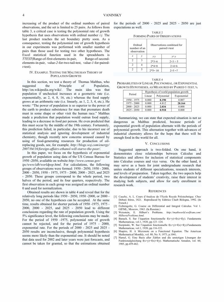
increasing of the product of the ordinal numbers of paired observations, and the set is limited to 25 pairs. As follows from table 3, a critical case is testing the polynomial rate of growth hypothesis that uses observations with ordinal number i·j. The last product reaches the set boundary pretty soon. As a consequence, testing the polynomial rate of growth hypothesis in our experiments was performed with smaller number of pairs than those used for testing two other hypotheses. The Excel statistical function used in the spreadsheets is TTEST(Range-of-first-elements-in-pair, Range-of-second-elements-in-pair, value-2-for-two-tail-test, value-1-for-paired-t-test).
IV. EXAMPLE. TESTING THE MALTHUSIAN THEORY OF POPULATION GROWTH
In this section, we test a theory of Thomas Malthus, who suggested the Principle of Population, http://en.wikipedia.org/wiki/. The main idea was that population if unchecked increases at a geometric rate (i.e. exponentially, as 2, 4, 8, 16, etc.) whereas the food supply grows at an arithmetic rate (i.e. linearly, as 1, 2, 3, 4, etc.). He wrote: “The power of population is so superior to the power of the earth to produce subsistence for man that premature death must in some shape or other visit the human race.” Malthus made a prediction that population would outrun food supply, leading to a decrease in food per person. He even predicted that this must occur by the middle of the 19th century. Fortunately, this prediction failed, in particular, due to his incorrect use of statistical analysis and ignoring development of industrial chemistry, though recently new concerns aroused caused by using of food-generating resources for production of oil- replacing goods, see, for example, http://blogs.wsj.com/energy/ 2007/04/16/foreign-affairs-ethanol-will-starve-the-poor/.
In this paper, we focus on the hypothesis of exponential growth of population using data of the US Census Bureau for 1950 -2050, available on website http://www.census.gov/ ipc/www/idb/worldpop.html. For calculations, the following groups of observations were formed: 1950 - 2050, 1950 - 2000, 2000 - 2050, 1950 - 1975, 1975 - 2000, 2000 - 2025, and 2025 - 2050. These groups correspond to the whole period, two halves of the period, and its four quarters, respectively. The first observation in each group was assigned an ordinal number 0 and used for normalization.
Obtained results are shown in table 4 and reveal that for the relatively long periods like 1950 - 2050, 1950 -2000, or 2000 - 2050, no one of the hypotheses can be accepted. At the same time, results obtained for shorter periods of 1950 -1975, 1975 -2000, 2000 - 2025, and 2025 - 2050 lead to different conclusions regarding the rate of population growth. Using the 5% significance level, the following conclusions may be made. For the period of 1950 -1975, polynomial rate of growth cannot be rejected, and for the period of 1975 - 2000, exponential rate. For the periods of 2000 - 2025 and 2025 - 2050 results are inconclusive, though polynomial hypothesis seems more likely than the exponential one. It should be noted that data used for 2002 and later years were just forecasts, and cannot be taken for granted, so that the estimations obtained
for the periods of 2000 - 2025 and 2025 - 2050 are just expectations as well.
TABLE 2 FORMING PAIRS OF OBSERVATIONS
Ordinal number of an observation Observations combined for paired t-test x y x·y x+y 2 3 2*3=6 2+3 = 5 2 4 2*4=8 2+4=6 2 5 2*5= 10 2+5 =7
TABLE 4
PROBABILITIES OF LINEAR, POLYNOMIAL, OR EXPONENTIAL
GROWTH HYPOTHESES, AS MEASURED BY PAIRED T-TEST, %
Period Hypothesis of world population growth Linear Polynomial Exponential
1950 - 1975 0.000 8.190 0.007 1975 - 2000 0.000 4.812 28.164 2000 - 2025 0.000 2.034 0.000 2025 - 2050 0.000 0.918 0.000
Summarizing, we can state that expected situation is not so dangerous as Malthus predicted, because periods of exponential growth of population alternate with the periods of polynomial growth. This alternation together with advances of industrial chemistry allows for the hope that there will be enough food in the world for all.
V. CONCLUSIONS
Suggested approach is two-folded. On one hand, it demonstrates close relationships between Calculus and Statistics and allows for inclusion of statistical components into Calculus courses and vice versa. On the other hand, it may serve as a basis for joint undergraduate research that unites students of different specializations, research interests, and levels of preparation. Taken together, the two aspects help the development of students’ creativity, raise their interest in studying both subjects, and allow for early enrollment in research work.
REFERENCES [1] Cauchy, A. L. Cours d’Analyse de l’Ecole Royale Polytechnique. Chez
Debure frères, 1821. Reproduced by Editrice Clueb Bologna, 1992. (In French.)
[2] Fichtengoltz, G. Course on Differential and Integral Calculus. Vol 1. GIFML, Moscow, 1963. (In Russian.)
[3] Weisstein, E. Hilbert’s Problems. http://mathworld.wolfram.com/ HilbertsProblems.html.
[4] Banach, S. Sur l’équation fonctionnelle f(x+y)=f(x)+f(y). Fundamenta Mathematicae, vol.1, 1920, pp.123 -124.
[5] Sierpinski, W. Sur l’équation fonctionnelle f(x+y)=f(x)+f(y).Fundamenta Mathematicae, vol.1, 1920, pp.116-122.
[6] Shapiro, H. A Micronote on a Functional Equation. The American Mathematical Monthly, vol. 80, No. 9, 1973, p.1041.
[7] Hamel, G. Eine Basis aller Zahlen und die unstetigen Lösungen der Funktionalgleichung f(x+y)=f(x)+f(y). Mathematische Annalen, vol. 60, 1905, pp.459-462.
VANINSKY 4

[8] Broggi, U. Sur un théorème de M. Hamel. L’Enseignement Mathématique, vol. 9, 1907, pp.385-387.
[9] Darboux, G. Sur la composition des forces en statique. Bulletin des Sciences Mathématiques, vol. 9, 1875, pp. 281-299.
[10] Darboux, G. Sur le théorème fondamental de la Géométrie projective. Mathematische Annalen, vol. 17, 1880, pp.55-61.
TABLE 3 SPREADSHEET EXAMPLE
NOTES: 1. Example. The formula in the cell corresponding to the
exponential rate of growth hypothesis is =TTEST(X14:X38,AA14:AA38,2,1). The result is 0.2816.
2. The spreadsheet is available from author upon request.
[11] Borwein, J., Bailey, D. and R. Girgensohn. Experimentation in Mathematics: Computational Paths to Discovery. Natick, MA: A. K. Peters, 2004.
[12] Edwards, H. and D. Penney. Calculus. 6th Ed. NJ: Prentice Hall, 2002. [13] Weiers, R. Introduction to Business Statistics. 4th Ed. CA: Wadsworth
Group. Duxbury/Thompson Learning, 2002.
Hypothesis testing for the rate of magnitude (linear, polynomial, exponential)Paired t-test
World population, 1975 - 2000.Sourse: http://www.census.gov/ipc/www/idb/worldpop.html
Adjust for actual #Obs!!! Adjust for actual #Obs!!! Adjust for actual #Obs!!!#Obs = 25 P{T-test 0.0000 P{T-test} 0.0481 P{T-tes 0.2816
St. Dev 246.3 252.4 St. Dev 0.0603 0.6262 St. Dev 0.0624 0.0618Norm Poly Avrg 810.6 837.5 Avrg 1.1600 0.8846 Avrg 1.2007 1.2004
4,155Norm LinLin Adj Linear Poly Adj Exp Adj Poly Exponential
1975 4,084 Xi=Ri-Norm Xi=Ri/No Xi=Ri/Norm# Raw data Xi i+j Xi+Xj (i+j) Xi+j Xi Xi i*j Xi*Xj (i*j) Xi*j (i*j) Xi*Xj (i+j) Xi+j
1 1976 4,154.7 71.0 2+3 356.5 5 363.3 1.0000 1.0174 2*3 1.0522 6 1.0885 2*3 1.0891 5 1.08902 1977 4,226.3 142.5 2+4 430.8 6 438.8 1.0172 1.0349 2*4 1.0704 8 1.1271 2*4 1.1079 6 1.10743 1978 4,297.7 214.0 2+5 505.9 7 517.9 1.0344 1.0524 2*5 1.0888 10 1.1658 2*5 1.1270 7 1.12684 1979 4,372.0 288.3 3+4 502.2 7 517.9 1.0523 1.0706 3*4 1.0885 12 1.2065 3*4 1.1267 7 1.12685 1980 4,447.1 363.3 2+6 581.3 8 599.0 1.0704 1.0890 2*6 1.1073 12 1.2065 2*6 1.1461 8 1.14676 1981 4,522.5 438.8 2+7 660.4 9 678.8 1.0885 1.1074 2*7 1.1266 14 1.2482 2*7 1.1661 9 1.16627 1982 4,601.6 517.9 3+5 577.3 8 599.0 1.1076 1.1268 3*5 1.1072 15 1.2693 3*5 1.1460 8 1.14678 1983 4,682.7 599.0 2+8 741.5 10 760.0 1.1271 1.1467 2*8 1.1465 16 1.2894 2*8 1.1867 10 1.18619 1984 4,762.5 678.8 3+6 652.7 9 678.8 1.1463 1.1662 3*6 1.1260 18 1.3289 3*6 1.1655 9 1.1662
10 1985 4,843.7 760.0 2+9 821.3 11 843.0 1.1658 1.1861 2*9 1.1660 18 1.3289 2*9 1.2069 11 1.206411 1986 4,926.8 843.0 4+5 651.6 9 678.8 1.1858 1.2064 4*5 1.1263 20 1.3675 4*5 1.1658 9 1.166212 1987 5,012.7 929.0 2+10 902.5 12 929.0 1.2065 1.2275 2*10 1.1859 20 1.3675 2*10 1.2275 12 1.227513 1988 5,099.3 1015.5 3+7 731.9 10 760.0 1.2273 1.2487 3*7 1.1457 21 1.3868 3*7 1.1859 10 1.186114 1989 5,185.7 1102.0 2+11 985.5 13 1015.5 1.2482 1.2699 2*11 1.2062 22 1.4058 2*11 1.2485 13 1.248715 1990 5,273.4 1189.7 3+8 813.0 11 843.0 1.2693 1.2913 3*8 1.1659 24 1.4431 3*8 1.2068 11 1.206416 1991 5,357.2 1273.5 4+6 727.0 10 760.0 1.2894 1.3118 4*6 1.1454 24 1.4431 4*6 1.1856 10 1.186117 1992 5,440.5 1356.8 2+12 1071.5 14 1102.0 1.3095 1.3322 2*12 1.2273 24 1.4431 2*12 1.2703 14 1.269918 1993 5,521.3 1437.6 2+13 1158.0 15 1189.7 1.3289 1.3520 2*13 1.2485 26 0.0000 2*13 1.2923 15 1.291319 1994 5,601.0 1517.3 3+9 892.8 12 929.0 1.3481 1.3715 3*9 1.1857 27 0.0000 3*9 1.2273 12 1.227520 1995 5,681.7 1597.9 4+7 806.2 11 843.0 1.3675 1.3913 4*7 1.1655 28 0.0000 4*7 1.2064 11 1.206421 1996 5,761.6 1677.9 2+14 1244.5 16 1273.5 1.3868 1.4109 2*14 1.2697 28 0.0000 2*14 1.3142 16 1.311822 1997 5,840.6 1756.8 5+6 802.1 11 843.0 1.4058 1.4302 5*6 1.1651 30 0.0000 5*6 1.2060 11 1.206423 1998 5,918.7 1835.0 3+10 974.0 13 1015.5 1.4246 1.4493 3*10 1.2060 30 0.0000 3*10 1.2482 13 1.248724 1999 5,995.6 1911.9 2+15 1332.2 17 1356.8 1.4431 1.4682 2*15 1.2911 30 0.0000 2*15 1.3364 17 1.332225 2000 6,071.7 1988.0 4+8 887.2 12 929.0 1.4614 1.4868 4*8 1.1860 32 0.0000 4*8 1.2276 12 1.2275
BRIDGING CALCULUS AND STATISTICS 5
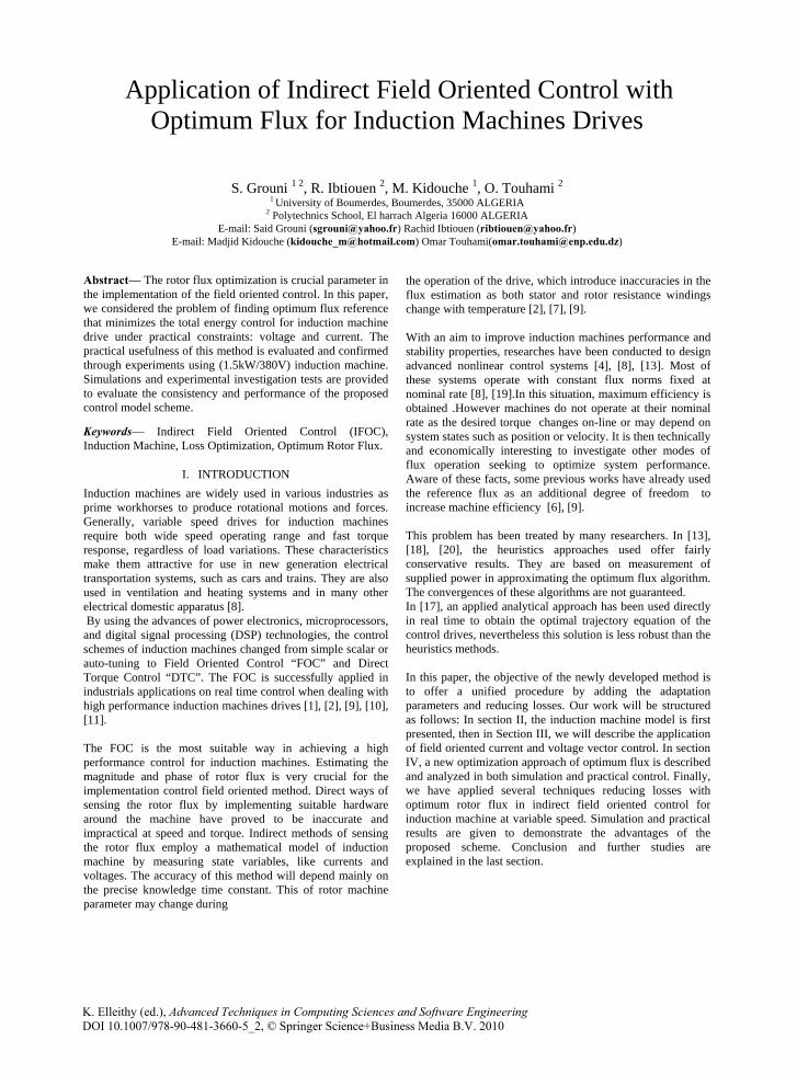
Abstract— The rotor flux optimization is crucial parameter in the implementation of the field oriented control. In this paper, we considered the problem of finding optimum flux reference that minimizes the total energy control for induction machine drive under practical constraints: voltage and current. The practical usefulness of this method is evaluated and confirmed through experiments using (1.5kW/380V) induction machine. Simulations and experimental investigation tests are provided to evaluate the consistency and performance of the proposed control model scheme. Keywords— Indirect Field Oriented Control (IFOC), Induction Machine, Loss Optimization, Optimum Rotor Flux.
I. INTRODUCTION Induction machines are widely used in various industries as prime workhorses to produce rotational motions and forces. Generally, variable speed drives for induction machines require both wide speed operating range and fast torque response, regardless of load variations. These characteristics make them attractive for use in new generation electrical transportation systems, such as cars and trains. They are also used in ventilation and heating systems and in many other electrical domestic apparatus [8]. By using the advances of power electronics, microprocessors, and digital signal processing (DSP) technologies, the control schemes of induction machines changed from simple scalar or auto-tuning to Field Oriented Control “FOC” and Direct Torque Control “DTC”. The FOC is successfully applied in industrials applications on real time control when dealing with high performance induction machines drives [1], [2], [9], [10], [11]. The FOC is the most suitable way in achieving a high performance control for induction machines. Estimating the magnitude and phase of rotor flux is very crucial for the implementation control field oriented method. Direct ways of sensing the rotor flux by implementing suitable hardware around the machine have proved to be inaccurate and impractical at speed and torque. Indirect methods of sensing the rotor flux employ a mathematical model of induction machine by measuring state variables, like currents and voltages. The accuracy of this method will depend mainly on the precise knowledge time constant. This of rotor machine parameter may change during
the operation of the drive, which introduce inaccuracies in the flux estimation as both stator and rotor resistance windings change with temperature [2], [7], [9]. With an aim to improve induction machines performance and stability properties, researches have been conducted to design advanced nonlinear control systems [4], [8], [13]. Most of these systems operate with constant flux norms fixed at nominal rate [8], [19].In this situation, maximum efficiency is obtained .However machines do not operate at their nominal rate as the desired torque changes on-line or may depend on system states such as position or velocity. It is then technically and economically interesting to investigate other modes of flux operation seeking to optimize system performance. Aware of these facts, some previous works have already used the reference flux as an additional degree of freedom to increase machine efficiency [6], [9]. This problem has been treated by many researchers. In [13], [18], [20], the heuristics approaches used offer fairly conservative results. They are based on measurement of supplied power in approximating the optimum flux algorithm. The convergences of these algorithms are not guaranteed. In [17], an applied analytical approach has been used directly in real time to obtain the optimal trajectory equation of the control drives, nevertheless this solution is less robust than the heuristics methods. In this paper, the objective of the newly developed method is to offer a unified procedure by adding the adaptation parameters and reducing losses. Our work will be structured as follows: In section II, the induction machine model is first presented, then in Section III, we will describe the application of field oriented current and voltage vector control. In section IV, a new optimization approach of optimum flux is described and analyzed in both simulation and practical control. Finally, we have applied several techniques reducing losses with optimum rotor flux in indirect field oriented control for induction machine at variable speed. Simulation and practical results are given to demonstrate the advantages of the proposed scheme. Conclusion and further studies are explained in the last section.
Application of Indirect Field Oriented Control with Optimum Flux for Induction Machines Drives
S. Grouni 1 2, R. Ibtiouen 2, M. Kidouche 1, O. Touhami 2 1 University of Boumerdes, Boumerdes, 35000 ALGERIA
2
E-mail: Said Grouni ( Polytechnics School, El harrach Algeria 16000 ALGERIA
[email protected]) Rachid Ibtiouen ([email protected]) E-mail: Madjid Kidouche ([email protected]) Omar Touhami([email protected])
K. Elleithy (ed.), Advanced Techniques in Computing Sciences and Software EngineeringDOI 10.1007/978-90-481-3660-5_2, © Springer Science+Business Media B.V. 2010

II. CONTROL PROBLEM FORMULATION A. Dynamic induction machine model Mathematical model of induction machine in space vector notation, established in d-q axis coordinates reference rotating system at sω speed can be represented in the Park’s transformation shown in Fig.1.
Fig.1. Scheme of Park transformation for induction machines Standard dynamic model of induction machine are available in the literature. Parasitic effects such as hysteresis, eddy currents, magnetic saturation, and others are generally neglected. The state-space model of the system equations related to the indirect method of vector control is described below. The reference frame with the synchronously rotating speed of sω , d-q-axis voltage equations are [15].
qssds
dssds dtdiRv ϕωϕ
−+= (1)
dssqs
qssqs dtd
iRv ϕωϕ
++= (2)
qrsdr
drr dtdiR ϕωωϕ )(0 −−+= (3)
drsqr
qrr )(dt
diR0 ϕωω
ϕ−++= (4)
Where sω , ω are the synchronous and rotor angular speeds. The stator and rotor fluxes are defined by the following magnetic equations:
drmdssdrdsmdslsds iLiLiiLiL +=++= )(ϕ (5)
qrmqssqrqsmqslsqs iLiLiiLiL +=++= )(ϕ (6)
dsmdrrdrdsmdrlrdr iLiL)ii(LiL +=++=ϕ (7)
qsmqrrqrqsmqrlrqr iLiL)ii(LiL +=++=ϕ (8)
lsL , lrL and mL are the stator leakage inductance, rotor leakage inductance, and mutual inductance, respectively. The expressions of electromagnetic torque and mechanical speed are stated by:
)( dsqrqsdrr
mem ii
LLpC ϕϕ −= (9)
ωϕϕωJfC
Jp)ii(
JLpL
dtd r
rdsqrqsdrr
m −−−= (10)
The difficulty of equation (9), is the strong coupling between flux and current of machine. B. Indirect Field Oriented Control (IFOC) For the rotor flux oriented control system, the rotor flux linkage vector has only the real component, which is assumed to be constant in the steady state. From (7) and (8), the rotor currents are given by:
( )dsmdrr
dr iLL1i −= ϕ (11)
( )qsmqrr
qr iLL1i −= ϕ (12)
Substituting (11) and (12) into (3) and (4), we can extract two expressions of dynamic d-q axis rotor flux components are expressed by:
0=−−+ qrsldsrr
mdr
r
rdr iRLL
LR
dtd
ϕωϕϕ
(13)
0iRLL
LR
dtd
drslqsrr
mqr
r
rqr =+−+ ϕωϕϕ
(14)
ωωω −= ssl is the slip angular speed If the vector control is fulfilled such that q-axis rotor flux can be zero, and d-axis rotor flux can be constant, the electromagnetic torque is controlled only by q-axis stator current, therefore from (9), with 0=qrϕ , 0=dri , yields
0dt
ddt
d qrdr ==ϕϕ
(15)
)( qsdrr
mem i
LLpC ϕ= (16)
Substituting (15) into (3) and (11)-(14) yields
qsr
mqr i
LL
i −= (17)
dsmdr iL=ϕ (18)
ds
qs
rdr
qs
r
msl i
iT1i
TL
==ϕ
ω (19)
where rrr RLT /= is the time constant of rotor, .
θω = with θ is the position of the rotor and ids , iqs
qrdr ϕϕ , are the direct and
quadrant axis components stator currents, where are the two–phase equivalent rotor flux linkages and the rotor speed ω is considered as state variable and the stator voltage vds , vqs
a
Vsa
θ
Vsb
Vsc
b
c
ira ir
c
irb
Vsd
Vsq
irq
ird
d
q
isd
isq
θs
as command variables. We have shown in equation (9) that the electromagnetic torque expression in the dynamic regime, presents the coupling
GROUNI ET AL. 8

between stator current and rotor flux. The main objective of the vector control of induction machine is, as in direct current (DC) machines, to control independently the torque and the flux [4]. This can be realized by using d-q axis rotating reference frame synchronously with the rotor flux space vector. The d-axis is aligned with the rotor flux space vector. Under this condition we have; rdr ϕϕ = and 0qr =ϕ . In this case the electromagnetic torque of induction machine is given by equation (16). It is understood to adjust the flux while acting on the component ids of the stator current and adjust the torque while acting on the iqs
)dt
dT(L1i *
r
*r
rm
*ds ϕ
ϕ+=
component. One has two variables of action then as in the case of a DC machine. Combining equations (13), (15) and (16) we obtain the following d-q-axis stator currents:
(20)
*
**
r
em
m
rqs
CpLLi
ϕ= (21)
∗
∗∗ =
r
qs
r
msl
iTL
ϕω (22)
The torque *emC and flux *
rϕ are used as references control and the two stator currents ids , iqs
*sl
r
*r
em RpC
2
ωϕ=∗
as inputs variables [13], [19]. Combining equations (21)-(22) we obtain the following expression of reference torque as a function of reference slip speed.
(23)
with **sls ωωω +=
The references voltages are given in steady state by: *qss
*s
*dss
*ds iLiRv σω−= (24)
*dss
*s
*qss
*qs iLiRv σω+= (25)
where σ is the total leakage coefficient given by:
rs
2m
LLL1 −=σ (26)
These equations are functions of some structural electric parameters of the induction machine (Rs, Rr, Ls, Lr, Lm
dtT
iLt
rr
qsms ∫
+=
0 ϕωθ
) which are in reality approximate values. The rotor flux amplitude is calculated by solving (19), and its spatial position is given by:
(27)
C. simulation Study of IFOC voltage and current Control A simulation study was carried out to investigate the following models controls used on a closed loop IFOC system which depend on the loading conditions. The current and voltage control simulations of IFOC are given by Fig.2 and Fig.3.
Fig. 2. Simulation of IFOC - IM drives with current control. Fig. 3. Simulation of IFOC-IM drives with voltage control. III. LOSS MINIMISATION IN IFOC INDUCTION MACHINE A- Power losses of induction machine In the majority constructions of induction machines, electromagnetic time constant is much smaller than mechanical time constant. For this reason the strategy of torque control which minimizes power losses can be reduced to the steady electromagnetic state. Several loss models are proposed and used in the literature, among this work those of [8], [9] and [10] which take into account the copper losses of the stator , the rotor windings and the iron losses. The total electrical input power of induction machine composed by resistive losses PR,loss, power P field stored as magnetic field energy in the windings and mechanical output power Pmech
( )
( ) ( )( ) ( )dsqsqsqr
r
mrdsqrqsdr
r
m
qrdrrqsdss
qrqr
drdr
r
qsqs
dsdsstotalel
iiiiL
LRiiLL
iiRiiR
dtd
dtd
Ldtdi
idt
diiLtP
+−−+
+−++
+−
+=
2
1
2222
,
ϕϕω
ϕϕ
ϕϕσ
expressed in the d,q variables. Applying the transformation to rotating reference frame on d,q variables the total power is given by:
(28)
This equation can be written in a condensed form as:
mechloss,Rfield
total,el PPdt
dPP ++= (29)
With:
0 0.5 1 1.5 2-200
-100
0
100
200
0 0.5 1 1.5 2
-50
0
50
0 0.5 1 1.5 2-0.5
0
0.5
0 0.5 1 1.5 20
0.5
1
1.5
0 0.5 1 1.5 2-20
-10
0
10
20
-1 -0.5 0 0.5 1-1
-0.5
0
0.5
1
Ω , Ωref (rd/s) Cem (N.m)
Φqr (wb) Φdr (wb)
Ia (A) Φα (wb)
Φβ (wb)
t (s)
t (s)
t (s) ( )
t (s)
t (s)
0 0.5 1 1.5 2-200
-100
0
100
200
0 0.5 1 1.5 2
-50
0
50
0 0.5 1 1.5 2-0.5
0
0.5
0 0.5 1 1.5 20
0.5
1
1.5
0 0.5 1 1.5 2-20
-10
0
10
20
-2 -1 0 1 2-2
-1
0
1
2
Ω , Ωref (rd/s) Cem (N.m)
Φqr (wb) Φdr (wb)
Ia (A) Φα (wb)
Φβ (wb)
t (s)
t (s)
t (s) ( )
t (s)
t (s)
APPLICATION OF INDIRECT FIELD ORIENTED CONTROL 9
( ) ( )2
qr2drr
2qs
2dssloss,R iiRiiRP +++= (30)
( ) ( )2qr
2dr
r
2qs
2ds
sfield L2
1ii2L
P ϕϕσ +++= (31)
( )dsqrqsdrr
mm ii
LL
P ϕϕω −= (32)
According to the equivalent diagrams, the model of iron losses is described by:
2m
2r
Fes
FeFe LRPP ϕ
∆∆ == (33)
B. Power loss minimization with level flux control
B.1 Optimization flux for copper loss minimization The flux optimization for minimized energy in steady state consists to find the optimal trajectory of flux, ∀ T ∈[ 0,T ], which minimizes the cost function. The optimum rotor flux calculation is given by the relation:
)( emr Cf=ϕ (34) According to the dynamic model induction machine, the total electrical power loss can be written:
( )
2
2
22
12
2
2
222
2
2
2r
emrrds
r
mr
m
rf
r
mrqsds
r
mrst
Ci
LLR
LR
LLR
iiLLR
RP
ϕβϕβϕ
ϕ
+=−
+++
+=∆
(35)
Optimum operation point, corresponding to the minimum loss is obtaining by setting:
( )0=
∂∆∂
r
tPϕ
(36)
The resolution of this equation, gives the optimum rotor flux:
emoptr Cβϕ = (37)
Where
( )4
1
2
22
++
=pRRLRRL
fs
mrsrβ (38)
This parameter depends on machine operating. From the equations (20) and (21) we deduce that the optimal control in the steady state is given by:
+= opt
rr
optr
m
ro
Tdtd
LTu ϕ
ϕ 11 (39)
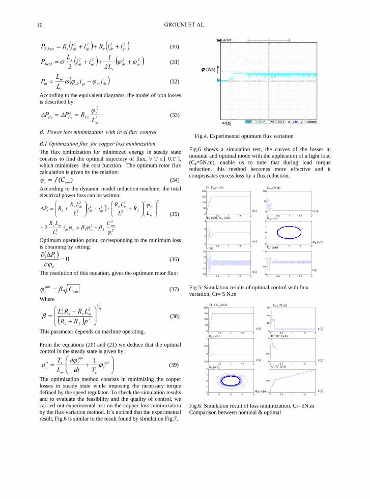
The optimization method consists in minimizing the copper losses in steady state while imposing the necessary torque defined by the speed regulator. To check the simulation results and to evaluate the feasibility and the quality of control, we carried out experimental test on the copper loss minimization by the flux variation method. It’s noticed that the experimental result, Fig.6 is similar to the result found by simulation Fig.7.
Fig.4. Experimental optimum flux variation
Fig.6 shows a simulation test, the curves of the losses in nominal and optimal mode with the application of a light load (Cr=5N.m), enable us to note that during load torque reduction, this method becomes more effective and it compensates excess loss by a flux reduction. Fig.5. Simulation results of optimal control with flux variation, Cr= 5 N.m
Fig.6. Simulation result of loss minimization, Cr=5N.m Comparison between nominal & optimal
0 0.5 1 1.5 20
50
100
150
200
0 0.5 1 1.5 2
0
50
100
0 0.5 1 1.5 2-2
0
2
4
-2 -1 0 1 2-2
-1
0
1
2
0 0.5 1 1.5 2-20
-10
0
10
20
0 0.5 1 1.5 20
0.5
1
1.5
t (s)
Ω , Ωref (rd/s) Cem (N.m)
Φdr (wb), Φqr (wb)
Φα (wb)
Ia (A) Φro (wb)
t (s) t (s)
t (s)
t (s)
Φβ (wb)
0 0.5 1 1.5 20
50
100
150
200
0 0.5 1 1.5 20
20
40
60
0 0.5 1 1.5 2-0.5
0
0.5
1
0 0.5 1 1.5 20
0.5
1
1.5
-2 -1 0 1 2-2
-1
0
1
2
0 0.5 1 1.5 20
0.5
1
Ω , Ωref (rd/s) Cem (N.m)
Φqr (wb) Φro, Φr
n (wb)
Φα (wb)
Pjo, Pj
n (p.u)
t (s) t (s)
t (s)
Φβ (wb)
t (s)
t (s)
GROUNI ET AL. 10

C. Copper loss minimization with ( )qsds ifi = The optimization loss is given by using the objective function linking two components of stator current for a copper loss minimization. The expression of power losses is given by:
( )222
qsdsrr
ms
dsdrrr
mqsqs
dsdsst
iiTL
LR
iLT
Ldt
dii
dtdi
iLP
+
++
−
+=∆ ϕσ
(40)
In steady state, the minimum of power losses is reached for:
qsrrs
mds i
TLRL
i2
12
1
+= (41)
The behavior of the machine is simulated by using the block diagram of figure 7. The simulation results are presented on figure 8 under light load application. This method shows an important decrease in copper losses under low load torque.
Fig.7. Simulation result of copper loss minimization, Cr=5N.m Comparison between nominal & optimal
D. Copper and iron loss minimization with ( )ω,qsds ifi = Loss Minimization is presented by introducing the mechanical phenomena. Copper and iron losses are given by:
( ) 222
222ds
fer
mqs
fer
Ferqsdsst i
RRL
iRR
RRiiRP
+−
+++=∆
ω (42)
( ) qsfersm
ferfesrsds i
RRRLRRRRRR
i+−
++= 22 ω
(43)
The simulation results of Fig.8 shows a faster response time speed.
Fig.8. Simulation result of copper and iron loss minimization, Cr=5N.m Comparison between nominal & optimal
IV. CONCLUSION In this work, we have presented a new method in reducing losses while considering and keeping under control machine parameters. This method could be important for the implementation in real time field oriented control. It has successfully demonstrated the design of vector field oriented control technique with optimum rotor flux using only the stator currents and position measurements. The main advantages of this method is that it is cheap and can be applied in both open and closed loop control.
0 0.5 1 1.5 20
50
100
150
200
0 0.5 1 1.5 2-20
0
20
40
60
0 0.5 1 1.5 2-1
0
1
2
-1 -0.5 0 0.5 1-1
-0.5
0
0.5
1
0 0.5 1 1.5 2-20
-10
0
10
20
0 0.5 1 1.5 20
0.5
1
t (s)
Ω , Ωref (rd/s) Cem (N.m)
Φdr (wb), Φqr (wb)
Φα (wb)
ias (A)
Pjo, Pj
n (p.u)
t (s) t (s)
t (s)
t (s)
Φβ (wb)
0 0.5 1 1.5 20
50
100
150
200
0 0.5 1 1.5 2-20
0
20
40
60
0 0.5 1 1.5 2-0.5
0
0.5
1
0 0.5 1 1.5 2-0.5
0
0.5
1
1.5
0 0.5 1 1.5 2-20
-10
0
10
20
0 0.5 1 1.5 20
0.5
1
Ω , Ωref (rd/s) Cem (N.m)
Φqr (wb) Φro, Φr
n (wb)
Isa(A)
Pj+ f o, Pj+ f
n (p.u)
t (s) t (s)
t (s)
t (s)
t (s)
t (s)
APPLICATION OF INDIRECT FIELD ORIENTED CONTROL 11

APPENDICE induction motor parameters: Pn= 1.5 kw, Un= 220 v, Ωn= 1420 tr/mn, In= 3.64 A(Y) 6.31A(Δ), Rs= 4.85Ω, Rr= 3.805Ω, Ls= 0.274 H, Lr= 0.274 H, p= 2, Lm= 0.258 H, J= 0.031 kg.m 2, fr= 0.008 Nm.s/rd.
REFERENCES [1] F. Abrahamsen, F. Blåbjer, J.K. Pederson, “Analysis of stability in low cost
energy optimal controlled PWM VSI fed induction motor drive” in Proc. EPE’97 Trondheim Norway 1997, pp. 3.717-3.723.
[2] F. Abrahamsen, “Energy optimal control of induction motors” Ph.D. dissertation, Aalborg University, institute of energy technology, 1999.
[3] A.S. Bezanella, R. Reginetto, “Robust tuning of the speed loop in indirect field oriented control induction motors” Journal Automatica, Vol. 03, 2001, pp. 1811-1818.
[4] F. Blaschke, “The principle of field orientation as applied to the new transvector closed loop control system for rotating field machines” Siemens review, Vol. 34, May 1972, pp. 217-220.
[5] B.K. Bose, Modern Power Electronics and AC Drives. 2002, Prentice Hall. [6] J. H. Chang, Byung Kook Kim,“ Minimum- time minimum – loss speed
control of induction motors under field oriented control ” IEEE Trans. on Ind. Elec. Vol. 44, No. 6, Dec. 1997
[7] A. El-Refaei, S. Mahmoud, R. Kennel, “Torque Ripple Minimization for Induction motor Drives with Direct Torque Control (DTC)” Electric Power Components & systems, vol. 33, No.8, Aug. 2005
[8] J. Faiz, M.B.B. Sharifian,“ Optimal design of an induction motor for an electric vehicle ” Euro. Trans. Elec. Power 2006, 16: pp.15-33
[9] Y. Geng, G. Hua, W. Huangang, G. Pengyi, “A novel control strategy of induction motors for optimization of both efficiency and torque response” in Proc. The 30th annual conference of IEEE Ind. Elect. Society, Nov2-6, 2004, Busan, Korea, pp. 1405-1410.
[10] S. Grouni, R. Ibtiouen, M. Kidouche, O. Touhami, “Improvement rotor time constant in IFOC induction machine drives” International Journal of Mathematical, Physical and Engineering Sciences IJMPES, Vol. 2, No.1, Feb. 2008, pp. 126-131.
[11] J. Holtz, “Sensorless control of Induction Machines- with or without Signal Injection?” Overview Paper, IEEE Trans. on Ind. Elect. , Vol. 53, No.1, Feb. 2006, pp. 7-30.
[12] J. Holtz, J. Quan, “Sensorless control of induction motor drives” Proceedings of IEEE, Vol.( 90), No.8, Aug. 2002, pp. 1359-1394.
[13] G.S. Kim, I.J. Ha, M.S. Ko, “Control of induction motors for both high dynamic performance and high power efficiency ” IEEE Trans. on Ind. Elect., Vol.39, No.4, 1988, pp. 192-199.
[14] I. Kioskeridis, N. Margaris, “Loss minimization in motor adjustable speed drives” IEEE Trans. Ind. Elec. Vol. 43, No.1, Feb. 1996, pp. 226-231. [14] R. Krishnan “Electric Motor Drives, Modeling, Analysis and control” 2001, Prentice Hall. [15] P. Krause, Analysis of electric Machinery, Series in Electrical Engineering, 1986, McGraw Hill, USA. [16] E. Levi, “Impact of iron loss on behavior of vector controlled induction machines” IEEE Trans. on Ind. App., Vol.31, No.6, Nov./Dec. 1995, pp. 1287-1296. [17] R.D. Lorenz, S.M. Yang, “AC induction servo sizing for motion control
application via loss minimizing real time flux control theory” IEEE Trans. on Ind. App., Vol.28, No.3, 1992, pp. 589-593.
[18] J.C. Moreira, T.A. Lipo, V. Blasko, “Simple efficiency maximizer for an adjustable frequency induction motor drive” IEEE Trans. on Ind. App., Vol.27, No.5, 1991, pp. 940-945.
[19] J. J. Martinez Molina, Jose Miguel Ramirez scarpetta,“ Optimal U/f control for induction motors” 15th Triennial world congress, Barcelona, Spain, IFAC 2002.
[20] M. Rodic, K. Jezernik, “Speed sensorless sliding mode torque control of induction motor” IEEE Trans. on Industry electronics, Feb. 25, 2002, pp.1-15.
[21] T. Stefański, S. Karyś, “Loss minimization control of induction motor drive for electrical vehicle” ISIE’96, Warsaw, Poland, pp. 952-957
[22] S.K. Sul, M.H. Park, “A novel technique for optimal efficiency control of a current-source inverter-fed induction motor” IEEE Trans. on Pow. Elec., Vol.3, No.2, 1988, pp. 940-945.
[23] P. Vas, Vector control of AC machines.1990, Oxford Science Publications.
GROUNI ET AL. 12

Urban Cluster Layout Based on Voronoi Diagram —— A Case of Shandong Province
ZHENG Xinqi WANG Shuqing FU Meichen ZHAO Lu
School of Land science and Technology,China University of Geosciences (Beijing)
Beijing 100083, China,telephone.+86-10-82322138;email:[email protected]
YANG Shujia
Shandong Normal University, 250014, Jinan, China
Abstract: The optimum layout of urban system is one of
important contents in urban planning. To make regional urban system planning more suitable to the requirements of urbanization development, this paper tests a quantitative method based on GIS & Voronoi diagram. Its workflows include calculating city competitiveness data, spreading the city competitiveness analysis by aid of spatial analysis and data mining functions in GIS, getting the structural characteristics of urban system, and proposing the corresponding optimum scheme of the allocation. This method is tested using the data collected from Shandong Province, China.
Keywords: City competitiveness;Spatial analysis;Voronoi Diagram;GIS;Optimum layout
1 INTRODUCTION
The urbanization level embodies comprehensively the city economic and social development level, and is the important mark that city--region modernization level and international competitiveness. Now facing the economical globalization, the cities increasingly becoming the core, carrier and platform of competition in the world.
No matter in a nation or in a region, constructing the urban platform with all strength, optimizing the urban system structure, developing the urban economy, advancing the urbanization level, all of these should be done well, which can strengthen the developing predominance and international competitiveness, further win the initiative in future. Completely flourishing rural economy and accelerating the urbanization course, which are the important contents and striving aims of constructing the well-off society completely that put forward in 16th Party Congress [1]. All of these should be considered from the region angle, and by planning the more reasonable regional urban system to be achieve.
The optimum layout of urban system is always an important content of urbanization construction and urban planning study. Many scholars have conducted studies on this aspect [2,3,4,5,6]. These researches considered more about
the urban space structure and evolution than its economic attraction, effectiveness and competitive superiority in the urban system, which did not consider the combined factors when conducting the urban system planning. To solve the problem, we tested a method and used the calculation data of urban competitiveness, by aid of the spatial analysis and data mining functions in GIS, Voronoi Diagram[7,8,9,10],then discussed the analysis and technical method about the optimizing scheme suggestion of urban system layout. Taking Shandong Province as an example and comparing with the past achievements, we found that the method in this paper is more scientifically reasonable.
2 DEFINING CITY COMPETITIVENESS
Competitiveness assessment is necessary in this competitive era. In urban system planning, we also need to think about the urban competitiveness assessment. Michael Porter suggested that the core of competitiveness be the concept of “Clusters” after he analyzed the comparative superiority theory in Nation Competitive Advantage [11]. In fact, the district which only possesses the superior natural resources will not become the prosperous district in the 21st century. The striding development will realize in some districts, which depend on the development of cluster (zone) to some degree.
The most influencing competitiveness assessment now in the world is WPY, founded by the World Economy Forum (WEF) and the Switzerland Lausanne international management and development college (IMD) in 1980. This assessment designed the integrated quantitative assessment index system according to the solid theoretical research with theoretical research, and began to take effect in 1989. The number of the assessment indices which are adopted at present reaches 314, and the number of nations and districts which are evaluated are up to 49. And 36 academic organizations and 3532 experts in the world are invited to participate in cooperating. Many organizations in China have had the research about competitiveness, such as the Renmin
K. Elleithy (ed.), Advanced Techniques in Computing Sciences and Software Engineering, DOI 10.1007/978-90-481-3660-5_3, © Springer Science+Business Media B.V. 2010

university of China, Institute of Finance and Trade Economics (IFTE) of the Chinese Academy of Social Sciences (CASS), Beijing LiYan Institute of Economics, city comprehensive competitiveness compare research center of Shanghai Academy of Social Sciences (SASS), School of Economics & Management of Southeast University, Guangdong Academy of Social Sciences (GDASS) and Hong Kong city competitiveness seminar etc. The most famous competitiveness evaluation in China at present is city competitiveness evaluation, Typical references include “Blue book of city competitiveness: report of the China city competitiveness” [12], “the concept and index system of city competitiveness” [13], and “the index system of China county-level economy basic competitiveness, China county-level economy basic competitiveness evaluation center, etc. Although there are a lot of evaluation methods about the city competitiveness at present, authoritative assessment index system and method has not been formed yet. In view of this, according to the needs of source and evaluation of data, we adopt a comparatively simple competitiveness index to weigh competitiveness.
The urban land is the carrier of all activities in a city. The city development is reflected by the change of the land to a great extent, and it is particularly true under the market economy condition. In order to study city competitiveness, we can take urban land as core and analyze the influencing factors, such as the maturity degree of urban land market and urban land use benefit, etc., and then indirectly evaluate the city competitiveness. If the urban land use condition is the result of the joint interaction of the nature, society, economy and market materials in a city, and if the urban land use benefit in a city is high, its city competitiveness generally is also comparatively high. So we analyzed and compared urban land assessment index system and city competitiveness evaluation system. We found that they have many similar contents, thus decided to use urban land evaluation results to reflect city competitiveness evaluation results, and called them the city competitiveness.
3 METHODS
The city competitiveness factors have great influence on the city development, and embody the city’s advantages of economic, social and natural conditions among cities. They are generally divided into two levels: factor and indictor.
3.1 SELECTION PRINCIPLE
(1) The changes of index have notable influence to city;
(2) The index values have clearer variable range;
(3) The index can reflect the differences among different quality cities;
(4) The indexes reflect the city development trend at present time; and have influence on city development in future.
(5) Making full use of the city statistical data which were published by national bureau of statistics of China;
(6) Adopting the non-statistics investigation data as much as possible that are collected by the authoritative organizations, like construction department and planning bureau etc.
3.2 METHOD OF EVALUATION SELECTION FACTORS
There are a lot of factors and indicators that influence the synthetic quality of urban land, which include macroscopic and microcosmic, static and dynamic, direct and indirect, and mutually contact and interaction. In order to select representative indices, adopting the following basic procedure: use the existing documents as reference, and investigate and analyze general factors and indicators that probably influence the urban land quality, finally select 82 indexes. Because it is not easy to procure effective data directly by part of the indexes, a total of 68 factors and indicators participate in the beginning of the analysis, then using SPSS10.0 to process principal components analysis. We obtain the principal components used in evaluation. The number of grading indexes is 58.
After removing the similar and repeated indexes, and extensively consulting experts across and outside the province, the final result is that the Shandong provincial city grading index system includes eight factors, 31 sub-factors and 58 indicators. The eight factors include: ① City location, including transportation location, external radiant capacity, urban built-up area; ② City concentration size, including population size, population density and the proportion of the secondary and tertiary industrial production value in GDP; ③ urban infrastructure conditions, including road traffic, water supply, gas supply, sewerage and heat supply; ④ Urban public service conditions, including school condition, medical and hygienic treatment condition; ⑤ Urban land use efficiency, including municipal service condition, capital construction investment intensity, the secondary and tertiary industrial increment intensity, trade intensity and labor input intensity; ⑥ City environmental conditions, including afforestation condition, waste treatment; ⑦ City economy development level, including GDP, financial condition, fixed assets investment condition, commerce activity condition, external trade activity condition and finance condition; ⑧ City development potential, including science and technology level, agriculture population per capita cultivated land and water resources condition etc.
3.3 IDENTIFYING THE WEIGHTS OF GRADING FACTORS
The weights of the grading factors and indicators were identified by five criteria: ① Weights are direct ratio to the
XINQI ET AL. 14

factors’ influence on land quality, which value between 0 and 1 and their sum is 1; ② Weight values of indicators that related with every evaluation factor vary from 0 to 1, and their sum is 1; ③ the invited experts should be related domain technologist, high level administrative decision-maker, who are familiar with urban land and society economy development condition as well as have higher authority. The total is 10 - 40 persons; ④ According to corresponding work background and marking demonstration, experts give mark, and they should independently mark without consulting.
According to the above principles and adopting Delphi method, we identified the weights of grading factors and indicators in Shandong provincial city competitiveness evaluation.
3.4 DATA PROCESSING
In the process of evaluating city competitiveness, datum involved and dimension among each index are different, so we firstly standardized the datum. There are many methods of data standardization. According to data characteristic and research purpose, we selected order standardization law. The formula is as follows:
where ijY is the score of indicator j of city i, ijX is the sequence of city i, which is gotten according to the value of indicator j of every city sequencing, and when the index is positive correlation with city competitiveness, the sequencing is for ascending order, otherwise for descending order. n is the number of evaluated cities.
The concrete process is as follows. Firstly, sequencing every index and counting its value, then counting sub-factors’ score through adopting the adding weights to sum method, taking the same step to count score of sub-factors. Finally we take adding weights to sum method to count synthetic score.
We calculated the index scores using the formula:
where ikF is the score of index k of city i; k jW is the weight of factor k corresponding with indicator j; i jY is the score of index i of city j; n is the number of indicators included in factor k.
We calculated the synthetic index scores by the formula:
where iS is the synthetic scores of grading object i; kW is the weight of factor k; ikF is the score of factor k of grading object i; n is the number of factors.
All the provincial cities get their total score respectively based on the calculation results of eight synthetic factors. What needs to be explained is that when taking the place order method to standard, for making the cities that participated in the competitiveness evaluation processes comparable, we carry on the unified standardization according to Shandong regionalism in 2001, which includes 17 cities, 31 county level cities, 60 counties and 12 independent and not entirely linking the piece areas under the jurisdiction of municipality, and amounting to 120 towns.
4 SPATIAL ANALYSIS METHOD
The spatial analysis originated from the “Computation Revolution” in geography and regional science in the 60’s. At the beginning stage, it chiefly applied quantitative (chiefly being statistic) methods to analyze the spatial distribution model of point, line and polygon (Hi Prof. Zheng, do you have any reference for this part? Thank you!). Afterwards, it even more emphasized the character of geographical space itself, spatial decision course and the temporal and spatial evolution course analysis of the complicated space system. In fact, from the map aooearance (what is aooearance?), people are carrying on all kinds of spatial analysis all the time consciously or unconsciously.
The spatial analysis is the general designation for analysis technology of spatial data. According to different data quality, it can be divided into: ① the analysis operation based on spatial graph data; ② the data operation based on non-spatial attribute; ③ combined operation of spatial and non-spatial data. The foundation that spatial analysis relies on is the geographical space database, and the mathematic means of its application including the logic operation, quantitative and statistical analysis, algebraic operation, etc. Its final purpose is to solve geographical space factual question that people encountered, draw and transmit geographical spatial information, especially implied information, and assist decision-making.
GIS is a science that integrates the newest technology of many disciplines, such as the relational database management, effective graphic algorithm, inserting value analysis, zoning and network analysis, which provides powerful spatial analysis tools and makes the complicated and difficult assignment become simple and easy to do. At present there are the spatial analysis functions in most GIS software. This
100 /ij ijY X n= ×
∑=
×=n
jjijkik YWF
1
)(
∑=
×=n
kikki FWS
1)(
URBAN CLUSTER LAYOUT BASED ON VORONOI DIAGRAM 15

article mainly depends on MapInfo Professional 7.0 [14] terrace, and uses the development languages such as Mapbasic [15] to carry on the function module developing, and realize the spatial analysis of competitive assessment in is the town. The process generalized in the following:
(1) digitize 1:500000 “Shandong district map” which is published by Shandong publishing company in the year 2001;
(2) establish a database for town space position and competitiveness power assessment index, and the connection by way of administration code establishment;
(3) build Voronoi Diagram[16], as shown in Fig.1;
Fig.1 Voronoi diagram of town in Shandong province
(4) Optimize the layout of the town cluster based on Voronoi diagram: calculating the amount of town cluster (zone) (such as 4、5、6、7、8 and so on), calculating the central position of the town cluster (zone) (which is called the center of mass in town cluster) using the total point value of town competition power as the weight of grading. It has the smallest sum of distance from the location to the surrounding towns. Through the trail, the amount of the center of mass chosen this time is 8, as shown in Fig. 2.
(5) use data mining technology to carry on spatial analysis and the knowledge discovery, serve as the new layout object with the group center of mass in town, and establish Voronoi diagram again. So we can obtain the scope of town cluster;
(6) establish competitiveness power evaluation picture (dividing the value with total points value and factor serves as the radius, and the seat is the centre of a circle with the town), which includes the total points value and factor branch value picture, as Fig. 2 and Fig. 3 show;
(7) optimize the layout based on optimizing principle, which means adjusting suitably on the contrary to the facts, like incorporation and displacement, etc., analyzing
competing power space analysis picture comparatively and making the final decision for the project of optimizing layout.
Fig.2 8 centers Voronoi diagram of town in Shandong province
Fig.3 spatial analysis of competition evaluation
5 DISTRIBUTION CHARACTERISTICS AND THE LAYOUT
OPTIMIZATION
According to the grand blue print that strides across the century of the planning “Development Report of National Economy and the Society of Distant View Objective Outline of 9th Five-Year Plan and in 2010 in Shandong” [17]: build the necessary mutually modernized town systems of four administrative levels in big or middle or small city and the villages and towns, and form four industry gathering zones Jiaoji, Xinshi, Dedong, Jingjiu based on heavy chemical industry bases and the high, new technology industry and three modernized agriculture areas each having its characteristic in the construction Jiaodong area coast, one of the warring states into which China was divided during the Eastern Zhou period, located in the southern portion of modern Shandong Province Central South mountain area and one of the warring states into which China was divided during
XINQI ET AL. 16

the Eastern Zhou period, located in the southern portion of modern Shandong Province northwest China plain are quickened to put into effect Huanghe River delta to develop and “at sea Shandong” to build two striding across the century the engineering greatly, and promote to economize entirely economical to realize division of labor reasonably, harmonious development in the high administrative levels.
According to the planning mentioned above, based on the Shandong province town Voronoi diagram, there are 5 town clusters (zone) of Shandong province by optimizing: the central Shandong Province town cluster ( Jinan, Taian, Zibo, Laiwu), the coastal town cluster (Qingdao, Wei Fang, Rizhao), peninsula town cluster (Yantai, Weihai), delta town cluster ( Dongying, Binzhou ), lake area town cluster (Jining, Linyi, Zaozhuang) and Jingjiu town cluster (Dezhou, He ze, Liaocheng ).
The five clusters (zone) cover 85.83% of 120 towns in Shandong province which is known from the competing power percentage of the five cluster (zone) (Fig. 4). The central Shandong town cluster has the strongest competing power, whose number of towns is placed in the middle, but the infrastructure, the efficiency of land use, the economy development level, the integrated strength are all at the first place in Shandong province. This region which aims to be the leader modern province capital in China pays more attention to develop high, new technological industry such as micro-electronics, precise engine instrument, new materials, fine chemical combination, biological project and so on, the third industry which is high level such as finance trade, business service, tourism and entertainment, science and technology consultation, higher education, science research, medical treatment, sanitation and so on by the aid of the persons with ability, developed traffic, the powerful foundation of economy technology in province capital. Industry diffusing and grads transfer should be done better especially with the chance of the region financial centre which Jinan has been made by the country. Solidify and improve the position of region centre, try best to build Jinan to be a modern integrated central city with multi-function.
Both the coastal town cluster and the lake area town cluster have their own characteristics. Qingdao is the central city in the coastal town cluster where the position condition of the town and the ecological environment are at the fist place all over the province. It is superior to other clusters for the lake area town on the centralizing scale of town, the infrastructure of town and the region develop potential. Qingdao is the central city in coastal town cluster which has the superior region position and perfect infrastructure, with the large opening, large economy and trade and extraversion. The coastal town cluster has the biggest port in Shandong and the town system with fine function which should make full use of being open to the outside in order to speed up the develop of the whole province, develop the economy and technology cooperation with other countries energetically, take part in international division of labor, catch the trends of the newest technology home and abroad, putting forth effort
development high and new technology industry and the export-oriented economy and makes hard this area become the whole nation to be open one of the highest and economic the strongest export-oriented economy region of Vigour of level. The lake area town cluster is with Jining for the center, and each town distributes in minute hill lake vicinity, and takes resource exploitation and the commodity trade as the major characteristic here is that Shandong develops the largest district of latent capacity in the 21st century.
0
5
10
15
20
25
30
35
amou
nt
posi
t ion
cent
r al i
zing
f oun
dat i
on
publ
i c u
se
l and
use
ecol
ogy
econ
omy
deve
l opm
ent
t ot a
l po
i nt s
cent r al shandong t own cl ust ercoast al t own cl ust erl ake ar ea t own cl ust erpeni nsul a t own cl ust erdel t a t own cl ust erj i ngj i u t own zone
Fig.4 the comparison of the optimum layout factors competing power in
Shandong province
The peninsula town cluster and the delta town cluster are two characteristic town clusters of Shandong. The focal point that crowd in delta town is a Shandong is built one of engineering, the very big result had been gained in the town infrastructure construction here, town economy development standard and town public installation constructions etc, the rich superiority of petroleum resource be fully given play to, and the industry made a good job of that the petroleum is processed and the petroleum is formed a complete set or system. At the same time, adopt the method that protection nature has developed, and positively develop using the natural resources such as wasteland etc, and develop petroleum replacement such as foodstuff and agriculture by-product process, salt chemical industry, machinery, builds the material,
URBAN CLUSTER LAYOUT BASED ON VORONOI DIAGRAM 17