1

ADVANCED THERMAL MOTOR PROTECTION USING DIGITAL RELAYS

Ed Lebenhaft, P.E. Calpine Corporation

Mark Zeller Schweitzer Engineering Laboratories, Inc.

ABSTRACT

The era of protecting rotating equipment using electromechanical devices has faded away. Today’s motor protection is accomplished with digital protective relays. Digital relays are multiphase, multifunction units that offer not only protection but also alarming, historical operational data, and communication to other microprocessor-based devices in a plant.

The most important facet in motor protection is the ability to accurately replicate heat flow into and out of a motor.

This paper discusses the dual first order thermal model and its superior ability to protect ac motors from overtemperature conditions during starting and running states.

INTRODUCTION

Digital relays are multiphase, multifunction microprocessor-based devices. With proper mechanical and electrical design precautions, these relays offer highly reliable and advanced protection of power system components. Any past protection limitations experienced in the world of electromechanical relays are no longer a factor. If a situation can be mathematically described, the microprocessor in a digital relay can be programmed to tackle that problem.

Because of the immense computing power of today’s microprocessors, digital relays offer additional, highly important features to complement protection. They alarm, store historical operating data about the protected equipment and the power system it is connected to, and communicate to other microprocessors in the plant, using a large selection of communications protocols. Digital relays are also miniature programmable logic controllers (PLCs). Relay protective elements, digital inputs, digital outputs, and analog quantities can be used in logic statements, generating custom control schemes to suit specific applications. Digital relays are no longer standalone protective devices. They can be incorporated into the overall manufacturing process in a plant.

The world of motor protection presents unique challenges. The most prominent challenge is modeling of motor temperature based on electrical current flow.

This paper discusses the dual first order thermal model, which is based on the thermodynamic laws of heat flow.

OVERVIEW OF THE FIRST ORDER THERMAL MODEL

FIGURE 1 illustrates the first order thermal model. The major components of the model are:

• Heat source. Heat flow from the source, I2r, is measured in watts (W).

• Thermal capacitance, Cth, which represents a motor with a thermal capacity to absorb heat from the heat source. The unit of thermal capacitance is W • s/°C.

• Thermal resistance, Rth, which represents the heat dissipated by a motor to its surroundings. The unit of thermal resistance is °C/W.

2

• Temperature, U. The unit of temperature is °C.

• Comparator, which compares the calculated motor temperature with a pre-set value based on the motor manufacturer’s data.

Heat Source

TRIP_+

U

Utrip

Cth Rth

Motor Heat Dissipation

( )+2 21 1 2 2I • r I • r

2I • r

FIGURE 1. First Order Thermal Model

The qualitative analysis of this model states that heat produced by the heat source is transferred to the motor, which in turn dissipates the heat to the surrounding environment.

The quantitative analysis is defined by a first order linear differential equation, similar to a parallel resistor-capacitor (RC) electrical circuit:

2th

th

dU UI r C •dt R

= + (W) (1)

where:

2

th

th

I r total heat flow (W)dUC • heat flow into motor (W)dt

U heat flow into surroundings (W)R

=

=

=

Motors comprise two major electrical components, stator and rotor. The stator produces a rotating magnetic field (at line frequency) in the air gap, inducing voltage in the rotor bars. This induced voltage produces current flow in the rotor bars. Rotor current produces a magnetic field of its own. The rotor magnetic field is at 90 degrees to the air-gap magnetic field, thus generating torque tangential to the rotor surface, resulting in rotational force, thus turning the shaft.

Because the construction of the stator and rotor is dissimilar, so are their thermal characteristics. To accommodate the difference in stator and rotor thermal properties, two separate thermal models are used to achieve greater accuracy:

1) Rotor model

a. Starting element – protects the rotor during the starting sequence.

b. Running element – protects the rotor when the motor is up to speed and running.

2) Stator model – protects the stator during starting and running.

Transition from one rotor element to the other occurs at 2.5 times the rated full-load current of the motor.

3

APPLYING FIRST ORDER THERMAL MODEL TO MOTOR STARTING

Starting an ac motor is considered an adiabatic (lossless) process.

Starting deposits a large amount of heat (magnitudes greater than rated heating) in the rotor bars. Also, the duration of the starting sequence is magnitudes shorter than motor thermal time constants. Thus, it is regarded that any heat deposited in the rotor will not dissipate to the surroundings during the starting sequence. It will dissipate later when the motor is up to speed and running, and air flows in the air gap.

Applying this assumption to the first order thermal model depicted in FIGURE 1, we are effectively stating that the thermal resistance of the rotor during starting is infinity (R = ∞). Substituting this condition into (1) yields:

2th th

dU U dUI • r C • C •dt dt

= + =∞

(W) (2)

Rearranging (2):

2

th

I • rdU • dtC

= (°C)

The thermal capacity of a motor is a physical attribute and does not change. Motor resistance is assumed to be constant at this point. Convert the above expression to per-unit (pu) quantity by substituting the following:

thr C 1 pu= =

Thus:

2dU I • dt=

Integrating the expression:

2 2dU I • dt I dt= =∫ ∫ ∫

The solution to this general integral is:

2U I • t= (pu °C) (3)

Motor manufacturers supply thermal limit information as part of motor data.

The starting thermal limit is expressed in terms of the maximum time (motor safe stall time) that corresponding locked-rotor current can be applied to a motor. Applying this to (3):

LRAI I= (pu locked rotor, amperes)

STALLt T= (safe stall time, seconds)

2trip LRA STALLU I • T= (pu °C) (4)

4

Incorporating the above into FIGURE 1 results in a rotor I2t starting element in FIGURE 2.

TRIP_+

CthHeat Source

Rth =

U

∞

2LRA STALLI • T

2I

FIGURE 2. Rotor I2t Starting Element

Plotting the pu temperature response of this model versus the line current of the motor, the response curve is a straight line, as illustrated in FIGURE 3.

Tem

pera

ture

(U/U

L), R

otor

R •

0.01

1.0

0.9

0.8

0.7

0.6

0.5

0.4

0.3

0.2

0.1

0

Cur

rent

10

9

8

7

6

5

4

3

2

1

00 5 10 15 20 25 30

Seconds

R1 = RM Constant

Rotor TemperatureU

Motor Current

Motor Torque

FIGURE 3. Rotor I2t Starting Element Response Curve

This model keeps the rotor resistance constant at RM, which occurs at standstill (S = 1.0) and is considered 1 pu.

HIGH-INERTIA STARTING

The rotor I2t starting element performs well except for high-inertia starts. A high-inertia start is when the time to accelerate a motor to rated speed is equal to or longer than its specified safe stall time.

When trying to use the I2t starting element in high-inertia cases, the starting thermal limit of 2LRA STALLI • T is

reached before the current drops below 2.5 • FLA, resulting in premature tripping of the motor, as shown in FIGURE 3. This would occur during every start. In other words, the motor cannot be started successfully. The solution is to use a speed switch.

The reluctance of many customers to use speed switches led to the development of a rotor starting element that dispenses with the use of a speed switch in a motor starting logic scheme, while providing reliable and accurate protection during this critical state.

5

INDUCTION MACHINE EQUIVALENT CIRCUIT

At the dawn of the twentieth century, an engineer and inventor named Charles Steinmetz created an equivalent circuit for induction machines. It is still the only equivalent circuit used today and is shown in FIGURE 4.

( )r1– S R S

S

FIGURE 4. Induction Machine Equivalent Circuit

A closer look at the circuit reveals several interesting observations that might not be obvious at first glance:

• The stator and magnetizing branches are always connected across the supply voltage; thus they are exposed to line frequency at all times. The numerical value of stator impedance is fixed.

• The rotor branch is not connected to the line voltage. Instead, it is exposed to the voltage induced by the air-gap magnetic field. This voltage frequency depends on how quickly rotor bars cut the magnetic field. The numerical value of rotor impedance varies with the induced voltage frequency. This frequency is the difference between the electrical frequency of the line voltage and the mechanical rotational speed of the rotor/shaft assembly. The difference is called slip, S.

• Rotor impedance is slip dependent.

• Magnetic flux (thus current) distribution in the rotor bar varies with rotor speed.

• At standstill, because of the intense air-gap magnetic field (function of the starting current), only a small portion of the rotor bar cross section conducts rotor current (FIGURE 5).

• At rated speed, most of the rotor bar cross section is used (FIGURE 5). This fact influences apparent rotor resistance, Rr.

• Rotor resistance at standstill is substantially larger than at rated speed.

• Rr is speed dependent, Rr(S). This particular phenomenon is the key ingredient that makes the slip-dependent thermal model possible.

Rated Slip = SDeep Bar Effect

Starting Slip = 1Skin Effect

Rr Changes With Rotor Speed

FIGURE 5. Rotor Bars Current Distribution

6

CALCULATING MOTOR SLIP

Let us calculate the input impedance of the induction machine equivalent circuit. After calculating and separating it into its real and imaginary components, the real part represents the input resistance of an induction machine.

Motor input resistance, R, is:

rS

R (S)R RA •S

= + (pu Ω) (5)

where:

RS = stator resistance

Rr(S) = rotor resistance

S = motor slip

A = 1.2 (empirical constant)

Reference [1] shows the detailed derivation of R. It also derives the expression for Rr(S) in terms of maximum rotor resistance, RM, which occurs at standstill (S = 1), and normal rotor resistance, RN, which occurs at rated motor speed (S = rated).

The expression is:

r M N NR (S) (R R ) •S R= − + (pu Ω) (6)

Substituting (6) into (5) and solving for S yields:

N

S M N

RS

A • (R R ) (R R )=

− − − (7)

Two quantities are required by the slip-dependent thermal model in order to calculate fixed parameters RS, RM, and RN:

FLS = full-load slip

LRQ = locked-rotor torque (at S = 1)

When FLS and LRQ are entered as set points, the algorithm automatically calculates RM and RN and stores them in nonvolatile memory.

The moment the motor is energized, the relay takes the first snapshot of motor input impedance, Z; extracts the real component, R; and calculates stator resistance, RS.

The equations for RM, RN, and RS are:

M 2LRQRLRA

= (pu Ω) (8)

RATEDN 2 2

FLA

Q •S 1• FLSR FLSI 1

= = = (pu Ω) (9)

MS M

RR R R 0.833• R1.2 •1

= − = − (pu Ω) (10)

7

Now, slip is solely a function of motor input resistance. Motor input resistance is measured and updated every four milliseconds. Slip is calculated every two line frequency cycles.

A case study using 2,250 HP induction motor data illustrates the relationship between motor input resistance, motor slip, and rotor resistance.

FIGURES 6, 7, and 8 clearly illustrate the close dependence of rotor resistance on motor slip that, in turn, is extracted from motor input resistance.

Tota

l R (p

u)

FIGURE 6. Motor Input Resistance During Starting

Slip

Seconds

1.0

0.9

0.8

0.7

0.6

0.5

0.4

0.3

0.2

0.1

00 5 10 15 20 25 30

FIGURE 7. Motor Slip During Starting

8

Seconds

0.024

0.022

0.02

0.018

0.016

0.014

0.01

0.012

0

Rot

or R

esis

tanc

e R

rpu

5 10 15 20 25 30

FIGURE 8. Rotor Resistance During Starting

MODIFYING THE STARTING ELEMENT

The final step in establishing the slip-dependent thermal model is incorporating the slip-dependent rotor resistance into the heat source of the thermal model shown in FIGURE 2.

As mentioned before, the standard starting thermal element assumes a constant rotor resistance of 1 pu across the entire speed range from standstill (S = 1) to rated speed at rated shaft output (S = FLS). That value is RM.

Let us express the slip-dependent resistance value, Rr(S), in terms of its maximum value, RM, and substitute it into the heat source equation:

2 2 r

M

R (S)W I • r I •

R= = (pu W) (11)

Breaking (11) down into positive- and negative-sequence components accommodates motor heating due to balanced current (positive sequence) and any current unbalance (negative sequence) that might be present.

2 2r1 r2TOTAL 1 2

M M

R (S) R (S)W I • I •

R R= + (pu W) (12)

Replacing the heat source of FIGURE 2 with (12) gives rise to the slip-dependent thermal model shown in FIGURE 9 [2].

2LRA STALLI • T

( ) ( )⎛ ⎞+⎜ ⎟⎜ ⎟

⎝ ⎠

1 22 21 2

M M

R S R SI • I •

R R

∞

FIGURE 9. Slip-Dependent Starting Element

9

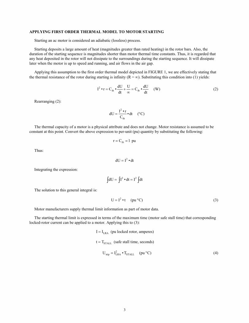
The response curve for this modified starting element is shown in FIGURE 10.

1.0

0.9

0.8

0.7

0.6

0.5

0.4

0.3

0.2

0.1

0

10

9

8

7

6

5

4

3

2

1

00 5 10 15 20 25 30

Seconds

Rotor Temperature

U

Motor Current

Motor Torque

Slip Dependent

R1 = (RM – RN)S + RN

FIGURE 10. Slip-Dependent Starting Element Response Curve

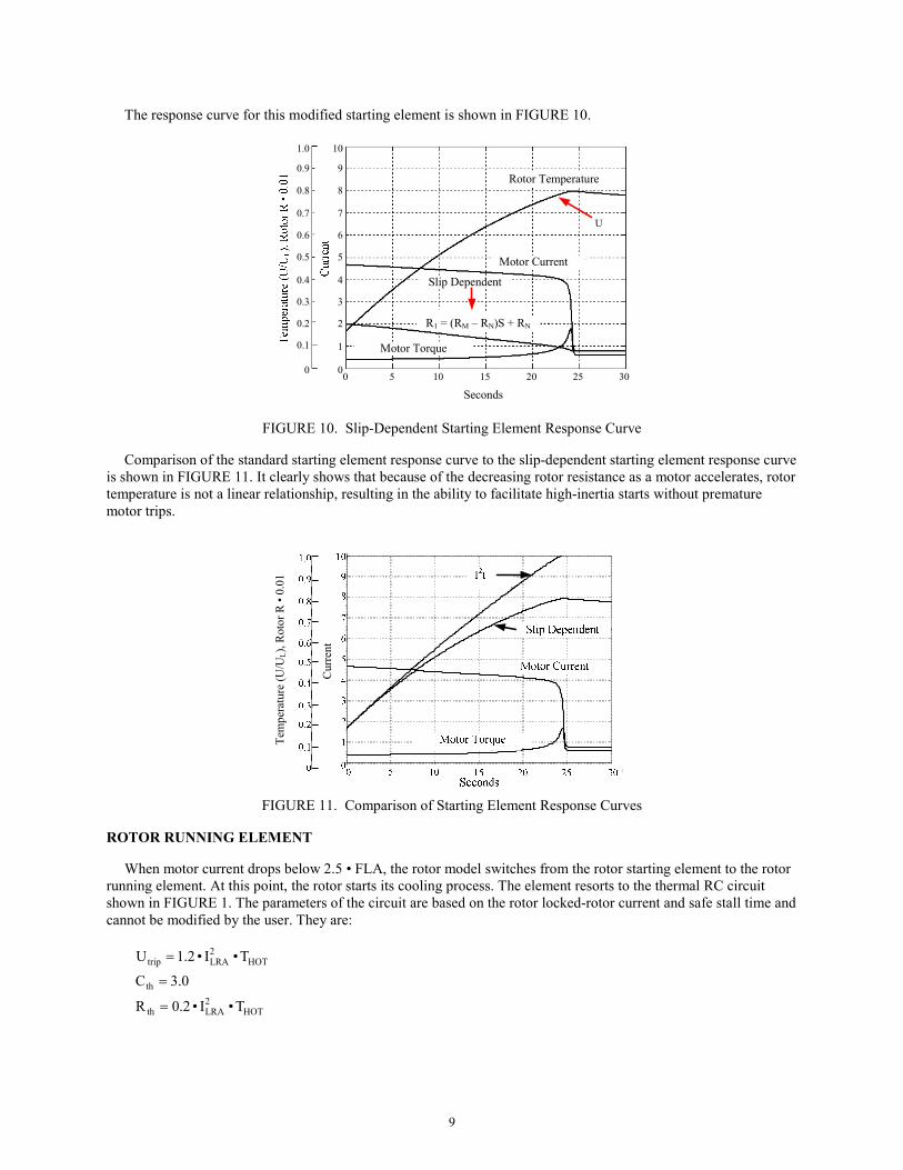
Comparison of the standard starting element response curve to the slip-dependent starting element response curve is shown in FIGURE 11. It clearly shows that because of the decreasing rotor resistance as a motor accelerates, rotor temperature is not a linear relationship, resulting in the ability to facilitate high-inertia starts without premature motor trips.

0 5 10 15 20 25 300

1

2

3

4

5

6

7

8

9

101.0

0.9

0.8

0.7

0.6

0.5

0.4

0.3

0.2

0.1

0

Tem

pera

ture

(U/U

L),R

otor

Rx

0.01

Rotor Temperature

layRetI2

Motor Current

Motor Torque

Seconds

Cur

rent

MOTOR TORQUE

MOTOR CURRENT

SECONDS

TEM

PER

ATU

RE

(U/U

L), R

OTO

R R

X 0

.01

CU

RR

ENT

SLIP DEPENDENT

I2t

Tem

pera

ture

(U/U

L), R

otor

R •

0.01

Cur

rent

FIGURE 11. Comparison of Starting Element Response Curves

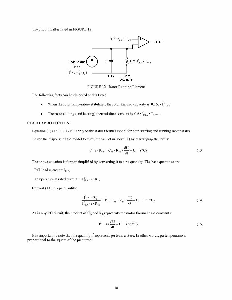
ROTOR RUNNING ELEMENT

When motor current drops below 2.5 • FLA, the rotor model switches from the rotor starting element to the rotor running element. At this point, the rotor starts its cooling process. The element resorts to the thermal RC circuit shown in FIGURE 1. The parameters of the circuit are based on the rotor locked-rotor current and safe stall time and cannot be modified by the user. They are:

2trip LRA HOT

th2

th LRA HOT

U 1.2 • I • T

C 3.0

R 0.2 • I • T

=

=

=

10

The circuit is illustrated in FIGURE 12.

2LRA HOT1.2 • I • T

2LRA HOT0.2 • I • T

( )+2 21 1 2 2I • r I • r

2I • r

FIGURE 12. Rotor Running Element

The following facts can be observed at this time:

• When the rotor temperature stabilizes, the rotor thermal capacity is 20.167 • I pu.

• The rotor cooling (and heating) thermal time constant is 2LRA HOT0.6 • I • T s.

STATOR PROTECTION

Equation (1) and FIGURE 1 apply to the stator thermal model for both starting and running motor states.

To see the response of the model to current flow, let us solve (1) by rearranging the terms:

2th th th

dUI • r • R C • R • Udt

= + (°C) (13)

The above equation is further simplified by converting it to a pu quantity. The base quantities are:

Full-load current = IFLA

Temperature at rated current = 2FLA thI • r • R

Convert (13) to a pu quantity:

2

2thth th2

FLA th

I • r • R dUI C • R • UdtI • r • R

= = + (pu °C) (14)

As in any RC circuit, the product of Cth and Rth represents the motor thermal time constant τ:

2 dUI • Udt

= τ + (pu °C) (15)

It is important to note that the quantity I2 represents pu temperature. In other words, pu temperature is proportional to the square of the pu current.

11

Equation (15) is a first order linear differential equation whose solution is:

t t

2 20U(t) I • e I • (1 e )

− −τ τ= + − (pu °C) (16)

where:

U(t) = pu temperature as a function of time

I0 = pu initial current

I = pu final current

τ = motor thermal running time constant

Another useful presentation of (16) to motor relay engineers is the time in which the thermal model will reach temperature.

Rewriting (16) yields:

2 2

02

I It • ln

I U(t)

⎡ ⎤−= τ ⎢ ⎥

−⎢ ⎥⎣ ⎦ (s) (17)

In plain language, (17) states that the time it takes to reach temperature is a function of the initial motor current, the final motor current, and the thermal running time constant.

Two important reminders are:

• The base for this pu system is motor full-load current, FLA.

• A valid range for pu temperature, U(t), is anywhere between initial pu temperature, 20I , and final pu

temperature, I2.

Let us further simplify (17) to make it more suitable for motor protection applications. Manufacturers state the machine’s service factor, SF, on every motor nameplate. Even though the exact interpretation of the SF varies, one thing is certain—any motor current greater than SF • FLA is considered a running overload condition. Translate this into a maximum pu temperature that the motor is designed for and can sustain at any time:

2FLAU(t) (SF• I )= (pu °C) (18)

Because IFLA = 1 pu, the above expression is further simplified to:

2U(t) SF= (pu °C) (19)

Substituting (19) into (17) results in the final equation of the first order thermal model:

2 2

02 2

I It • ln

I SF

⎡ ⎤−= τ ⎢ ⎥

−⎢ ⎥⎣ ⎦ (s) (20)

12

FIGURE 13 illustrates the stator model.

2I( )+2 2

1 2I I

FIGURE 13. Stator Model

A closer examination of (20) reveals that in order for time to be a rational number, the overload current, I, has to be greater than SF • IFLA. The question then is: what happens in a case where I is less than SF • IFLA? This situation does not constitute an overload condition but rather reflects the element’s response to a load change.

Let us revisit (17). Because the denominator has to be greater than zero to maintain a rational number, postulate (using the three time constants rule, which states that it takes three time constants for a quantity to exponentially decay to less than 5 percent of its original) that once the pu temperature, U(t), reaches within 5 percent (0.05 pu) of the final pu temperature, I2 (increasing or decreasing), the equation is satisfied.

2I U(t) 0.05− = (pu °C) (21)

Substituting (21) into (17) and again accounting for increasing or decreasing loads, t is the time it will take the motor temperature to change from 2

0I to I2:

( )2 2

0 2 20

I It • ln • ln 20 • I I

0.05

⎡ ⎤−⎢ ⎥= τ = τ −⎢ ⎥⎣ ⎦

(s) (22)

MOTOR STOPPED STATE

When a motor is de-energized, it does not require protection per se; however, it does need to be locked out and not allowed to re-energize until it cools down sufficiently to offer further service.

When current ceases to flow in the thermal circuit shown in FIGURE 1, the circuit reconfigures, as illustrated in FIGURE 14.

FIGURE 14. Motor Stopped State

The lockout state has the logic value of one only when U > URESET. Otherwise, it is zero.

13

The lockout time can be calculated by substituting the following values into (17):

2

20

RESET

I 0

I %TCU(t) %TC

COOLTIME3

=

=

=

τ =

Which leads us to lockout time, TLOCKOUT:

LOCKOUTRESET

COOLTIME %TCT • ln3 %TC

⎛ ⎞= ⎜ ⎟

⎝ ⎠ (s) (23)

This equation applies to the rotor and stator models.

THERMAL MODEL RESPONSE CURVES

The above presentation of the first order thermal model provides the mathematical derivations to substantiate equations that constitute the dual first order thermal model. Just as important and probably more practical is the graphical representation of the dual first order thermal model. This set of curves and the motor manufacturer’s thermal limit curves can be plotted together on a single graph to ensure that the model’s settings do indeed protect the motor to the motor manufacturer’s design specifications.

FIGURE 15 is a typical set of curves describing the response of the dual first order thermal model. The slip-dependent element of the rotor model is not shown because it is a dynamic algorithm fed by the actual measured input impedance of the motor (used to calculate rotor slip and resistance).

FIGURE 15. First Order Model Response Curves

14

CONCLUSION

Using the dual first order thermal model offers an accurate, thermodynamically based method of tracking pu temperature of an ac motor. Starting or running, the dual first order thermal model provides a superior replica of motor pu temperature generated by motor current flow, ensuring that motor manufacturer’s specifications are not exceeded, thus preserving the integrity and design life of the machine.

REFERENCES

[1] S. Zocholl, “Optimizing Motor Thermal Models,” proceedings of the 53rd Annual Petroleum and Chemical Industry Conference, Philadelphia, PA, September 2006.

[2] S. Zocholl, AC Motor Protection, Schweitzer Engineering Laboratories, Inc., 2003.

VITAE

Ed Lebenhaft received his BS in Electrical Engineering from the University of Toronto in 1972. He spent 18 years with Ontario Hydro, operating, then constructing, and finally designing nuclear power plants. In the following 14 years, Ed was a regional manager with Multilin Inc. (later bought out by GE). After a brief retirement, Ed joined Schweitzer Engineering Laboratories, Inc. as a field application engineer dealing primarily with motor protection. In September 2008, Ed joined Calpine Corporation as a relay technical advisor. Ed is a registered Professional Engineer in South Carolina.

Mark Zeller received his BS in Electrical Engineering from the University of Idaho in 1985. He has broad experience in industrial power system maintenance, operations, and protection. Upon graduating, he worked over 15 years in the pulp and paper industry, working in engineering and maintenance with responsibility for power system protection and engineering. Prior to joining Schweitzer Engineering Laboratories, Inc. in 2003, he was employed by Fluor to provide engineering and consulting services. He has been a member of IEEE since 1985.

© 2008 Doble Engineering Company – Revolutionary Machines Seminar All rights reserved. 20081006 • TP6338