advanced transceiver design for continuous phase...
TRANSCRIPT

ADVANCED TRANSCEIVER DESIGN FOR CONTINUOUS PHASE
MODULATION
by
Barıs Ozgul
B.S., Electrical and Electronics Engineering, Bogazici University, 1998
M.S., Electrical and Electronics Engineering, Bogazici University, 2002
Submitted to the Institute for Graduate Studies in
Science and Engineering in partial fulfillment of
the requirements for the degree of
Doctor of Philosophy
Graduate Program in
Bogazici University
2008

ii
ADVANCED TRANSCEIVER DESIGN FOR CONTINUOUS PHASE
MODULATION
APPROVED BY:
Prof. Hakan Delic . . . . . . . . . . . . . . . . . . .
(Thesis Supervisor)
Assist. Prof. Mutlu Koca . . . . . . . . . . . . . . . . . . .
(Thesis Co-supervisor)
Assoc. Prof. Fatih Alagoz . . . . . . . . . . . . . . . . . . .
Prof. Umit Aygolu . . . . . . . . . . . . . . . . . . .
Prof. Aysın Ertuzun . . . . . . . . . . . . . . . . . . .
Prof. Bulent Sankur . . . . . . . . . . . . . . . . . . .
DATE OF APPROVAL: 12.02.2008

iii
ACKNOWLEDGEMENTS
First of all, I would like to thank Prof. Hakan Delic and Assist. Prof. Mutlu Koca
for their invaluable help, encouragement, and support which made the accomplishment
of this dissertation possible.
I am also thankful to the commitee members, namely, Prof. Aysın Ertuzun, Prof.
Umit Aygolu, Prof. Bulent Sankur, and Assoc. Prof. Fatih Alagoz for their important
contributions.
I would like to thank my friends and colleagues, especially Ersen Ekrem, Nazlı
Guney, Cumhur Ozan Yalcın, Helin Dutagacı, Ender Konukoglu, Celal Esli, Erdem
Yoruk, and Ugur Bozkaya for their help and understanding.
I could not succeed without the support of my family. I would like to thank my
father, Dr. Ali Rıza Ozgul, and my brother, Dr. Alper Ozgul, who still continue to
stand beside me anytime I need. I would also like to thank the members of Satıoglu
family for their encouragement.
A special thank you goes to Ulgen Satıoglu. I will always be grateful for your
outstanding display of patience. A short break with you was enough to make long
hours of work bearable. Thank you for being so special.
Finally, I would like to dedicate this dissertation to my mother Sabriye Ozgul.
Only thing I can do is to thank you very much for all those priceless things you did for
me. I will always try to keep your memory alive.
This dissertation was partly supported by the Scientific and Technical Research
Council of Turkey (TUBITAK) Integrated Doctorate Program (BDP), the Bogazici
University Research Fund under Contracts 04HA201 and 06A204D, and the TUBITAK
KARIYER Research Projects Fund under Contract 105E077.

iv
ABSTRACT
ADVANCED TRANSCEIVER DESIGN FOR
CONTINUOUS PHASE MODULATION
This dissertation proposes advanced transceiver designs applying turbo and
space-time (ST) concepts to continuous phase modulation (CPM), which is preferred in
numerous power- and band-limited communication systems for its constant envelope
and spectral efficiency. Despite its highly attractive spectral properties, maximum-
likelihood detection of CPM over the frequency-selective multipath fading channels
can bring impractical complexity issues because of the intensive search over a single
super trellis which combines the effects of the modulation and the multipath channel.
Application of the reduced-state trellis search algorithms results in lower complexity
but the computational load could still be prohibitively large to obtain high perfor-
mance in long channel impulse responses. In the dissertation, instead of employing
trellis-based combined detection methods, equalization and demodulation functions
are separated and novel low-complexity receivers with soft-input soft-output (SISO)
time-domain and frequency-domain linear equalizers are proposed for bit-interleaved
coded CPM, which attain near-optimal performance by applying turbo processing. In
the proposed receivers, the front-end soft-information-aided linear equalizer is followed
by a central SISO CPM demodulator and a back-end SISO channel decoder where
double turbo processing is employed by performing back-end demodulation/decoding
iterations per each equalization iteration to improve the a priori information for the
front-end equalizer. Performance for the frequency-domain equalization is further im-
proved by proposing an orthogonal ST block coding scheme for CPM. The proposed
technique maintains the constant envelope and the phase continuity of the CPM wave-
forms perfectly by using appropriate tail symbols and, therefore, has no impact on the
spectral efficiency. Depending on the orthogonality of the ST combining, frequency-
domain equalization is applied as in the case of single antenna transmissions without
v
any increase in the computational load. In the dissertation, the receiver complexity is
reduced further by transferring all the equalization functions to the transmitter and
employing pre-equalization. For precoding the CPM signals on multipath fading chan-
nels while maintaining the spectral efficiency, a novel ST pre-equalizer is proposed,
limiting the envelope variations and attaining a peak-to-average power ratio that is
close to one by using a transmit selection diversity scheme.

vi
OZET
SUREKLI EVRE KIPLENIMI ICIN GELISMIS
ALICI-VERICI TASARIMI
Surekli evre kiplenimi (CPM) sabit zarfı ve spektral verimliliginden dolayı pek
cok guc ve bant kısıtlı iletisim sisteminde tercih edilmistir. Bu tezde ozyinelemeli ve
uzay-zaman (ST) yontemlerden faydalanılarak CPM icin gelismis alıcı-verici tasarımları
onerilmektedir. Dogrusal kiplenimlerden farklı olarak CPM sinyallerinin olusturulması
bir sonlu otomat tarafından gerceklestirilmekte olup bu sonlu otomattaki durum sayısı
kiplenimin hafıza buyuklugu, kiplenim indisinin degeri ve sembol alfabesinin boyu-
tuyla belirlenmektedir. Sagladıgı ustun spektral verimlilige ragmen CPM’nin cok yollu
frekans secici kanallar uzerinden en buyuk olabilirlik kestirimi kiplenim ve cok yollu
kanal hafızalarının birlesimini goz onune alan bir super kafes uzerinde yurutulen yogun
islemlere dayanmaktadır. Bu durum alıcıda pratik boyutların ustunde islemsel hacime
neden olabilmektedir. Durum azaltılmıs kafes arastırma algoritmalarının kullanımı
bu karmasıklıgı belli bir olcude azaltmakla birlikte uzun kanal durtu yanıtları soz
konusu oldugunda problem devam etmektedir. Bu tezde bit serpistirilmis CPM icin
kafes tabanlı yontemler uygulamak yerine denklestirme ve geri kiplenim islemlerini bir-
birinden ayıran ve yumusak-girdi yumusak-cıktı (SISO) ozellikli zaman- veya frekans-
bolgesel dogrusal denklestiriciler kullanan ozyinelemeli alıcılar onerilmekte ve uygu-
lanan donguler sayesinde en iyi basarıma yakın basarımlar elde edilmektedir. Onerilen
alıcılarda on kısımda bir SISO dogrusal denklestirici bulunmakta ve bu denklestiriciyi
SISO ozellikli geri kipleyici ve kanal kod cozucu takip etmektedir. Her denklestirici
dongusunden sonra geri kipleyici ve kanal kod cozucu arasında donguler kosturularak
bir sonraki denklestirme dongusu icin on bilgi gelistirilmekte ve bu uygulama sonucu
az karmasıklıkla yuksek basarım elde edilmektedir. Onerilen frekans-bolgesel alıcının
basarımı bir ST blok kodlama yontemi uygulanarak daha da arttırılmıstır. Soz konusu
ST blok kodlama yontemi CPM’nin sabit zarf ve surekli evre ozelliklerine bir etki

vii
yapmadıgından spektral verimlilik aynen korunmustur. Ayrıca uygulanan ST blok
kod ortogonal oldugundan dolayı alıcıda herhangi bir yapısal degisiklige veya islemsel
artısa neden olmamaktadır. Alıcı karmasıklıgının daha da azaltılması amacıyla veri-
cide ondenklestirme uygulanması bir diger arastırma konusu olarak ele alınmaktadır.
Bu calısma sonucunda CPM’nin spektral verimliligi korunarak ondenklestirilmesi icin
zarf degisintilerini kısıtlayan ve tepeden ortalamaya guc oranını bire yaklastıran bir ST
ondenklestirme yontemi onerilmektedir.

viii
TABLE OF CONTENTS
ACKNOWLEDGEMENTS . . . . . . . . . . . . . . . . . . . . . . . . . . . . . iii
ABSTRACT . . . . . . . . . . . . . . . . . . . . . . . . . . . . . . . . . . . . . iv
OZET . . . . . . . . . . . . . . . . . . . . . . . . . . . . . . . . . . . . . . . . . vi
LIST OF FIGURES . . . . . . . . . . . . . . . . . . . . . . . . . . . . . . . . . x
LIST OF TABLES . . . . . . . . . . . . . . . . . . . . . . . . . . . . . . . . . . xiii
LIST OF SYMBOLS/ABBREVIATIONS . . . . . . . . . . . . . . . . . . . . . xiv
1. INTRODUCTION . . . . . . . . . . . . . . . . . . . . . . . . . . . . . . . . 1
1.1. Background and Motivation . . . . . . . . . . . . . . . . . . . . . . . . 1
1.2. Literature Review and Research Contributions . . . . . . . . . . . . . . 2
1.3. Outline of Thesis . . . . . . . . . . . . . . . . . . . . . . . . . . . . . . 7
2. RESEARCH PRELIMINARIES . . . . . . . . . . . . . . . . . . . . . . . . . 11
2.1. Signal Model . . . . . . . . . . . . . . . . . . . . . . . . . . . . . . . . 11
2.1.1. Continuous Phase Modulation . . . . . . . . . . . . . . . . . . . 11
2.1.2. Approximation Methods for CPM . . . . . . . . . . . . . . . . . 16
2.2. Trellis Search Methods and Convergence Analysis for Turbo Decoding . 18
2.2.1. BCJR and Log-BCJR Algorithms . . . . . . . . . . . . . . . . . 20
2.2.2. Demodulation of CPM Using Log-BCJR Algorithm . . . . . . . 27
2.2.3. Convergence Analysis using EXIT Charts . . . . . . . . . . . . 29
2.2.4. Convergence Analysis for Iterative Demodulation of CPM . . . 31
3. DOUBLE TURBO EQUALIZATION OF CPM WITH TIME DOMAIN PRO-
CESSING . . . . . . . . . . . . . . . . . . . . . . . . . . . . . . . . . . . . . 35
3.1. Doubly-Iterative Equalization with Time Domain Processing . . . . . . 36
3.1.1. Receiver Overview . . . . . . . . . . . . . . . . . . . . . . . . . 37
3.1.2. SIC/MMSE TDE . . . . . . . . . . . . . . . . . . . . . . . . . . 40
3.1.3. Complexity Comparison . . . . . . . . . . . . . . . . . . . . . . 45
3.2. EXIT Chart Analysis . . . . . . . . . . . . . . . . . . . . . . . . . . . . 46
3.3. Simulation Results . . . . . . . . . . . . . . . . . . . . . . . . . . . . . 54
4. DOUBLE TURBO EQUALIZATION OF CPM WITH FREQUENCY DO-
MAIN PROCESSING . . . . . . . . . . . . . . . . . . . . . . . . . . . . . . 58

ix
4.1. Doubly-Iterative Equalization with Frequency Domain Processing . . . 60
4.1.1. Receiver Overview . . . . . . . . . . . . . . . . . . . . . . . . . 62
4.1.2. SIC/MMSE FDE . . . . . . . . . . . . . . . . . . . . . . . . . . 63
4.1.3. Complexity Comparison . . . . . . . . . . . . . . . . . . . . . . 65
4.2. EXIT Chart Analysis . . . . . . . . . . . . . . . . . . . . . . . . . . . . 69
4.3. Simulation Results . . . . . . . . . . . . . . . . . . . . . . . . . . . . . 74
5. ORTHOGONAL ST BLOCK CODING OF CPM ON MULTIPATH FADING
CHANNELS . . . . . . . . . . . . . . . . . . . . . . . . . . . . . . . . . . . . 78
5.1. Orthogonal ST Block Coding of CPM for Frequency-Domain Equalization 79
5.1.1. ST Block Coding for CPM . . . . . . . . . . . . . . . . . . . . . 80
5.1.2. Frequency-Domain Equalization for ST Block-Coded CPM . . . 85
5.2. Simulation Results . . . . . . . . . . . . . . . . . . . . . . . . . . . . . 86
6. ST PRE-EQUALIZATION OF CPM ON MULTIPATH FADING CHANNELS 90
6.1. Space-Time Pre-Equalization of Continuous Phase Modulation . . . . . 92
6.2. Analyses for the Error Performance and the Number of Antennas . . . 99
6.2.1. Upper Bound on the Error Performance . . . . . . . . . . . . . 99
6.2.2. Analysis for the Number of Antennas . . . . . . . . . . . . . . . 102
6.3. Simulations . . . . . . . . . . . . . . . . . . . . . . . . . . . . . . . . . 103
7. CONCLUSIONS . . . . . . . . . . . . . . . . . . . . . . . . . . . . . . . . . 112
APPENDIX A: MEAN CPM SIGNALS BASED ON BIT PROBABILITIES . 114
APPENDIX B: MMSE FILTER COEFFICIENTS FOR SIC/FDE . . . . . . . 116
APPENDIX C: TIME-REVERSED CPM SIGNALS . . . . . . . . . . . . . . 118
REFERENCES . . . . . . . . . . . . . . . . . . . . . . . . . . . . . . . . . . . . 120

x
LIST OF FIGURES
Figure 2.1. Turbo decoding of serially concatenated convolutional codes . . . . 20
Figure 2.2. Receiver EXIT charts for the turbo demodulation and decoding of
coded CPM . . . . . . . . . . . . . . . . . . . . . . . . . . . . . . 32
Figure 2.3. BER performance for the turbo demodulation and decoding of
coded CPM . . . . . . . . . . . . . . . . . . . . . . . . . . . . . . 33
Figure 3.1. The transmitter for the bit-interleaved coded CPM and the channel 36
Figure 3.2. Doubly-iterative receiver with TDE . . . . . . . . . . . . . . . . . 37
Figure 3.3. Transfer characteristics of the doubly-iterative receiver . . . . . . . 46
Figure 3.4. Transfer characteristic curves for the SIC/TDE at Eb/N0 = 3 and
6 dB . . . . . . . . . . . . . . . . . . . . . . . . . . . . . . . . . . 48
Figure 3.5. Comparison of the simulated trajectories and the characteristic
curves for the TDE and the demodulator at Eb/N0=3 dB . . . . . 50
Figure 3.6. EXIT chart analysis for the back-end iterations of the doubly-
iterative receiver with TDE . . . . . . . . . . . . . . . . . . . . . . 52
Figure 3.7. Analysis for the front-end and back-end iterations of the doubly-
iterative receiver with TDE . . . . . . . . . . . . . . . . . . . . . . 53
Figure 3.8. BER performance for no ISI, Proakis’ A channel, and channel I . . 55
Figure 3.9. BER performance in channels I and II . . . . . . . . . . . . . . . . 56

xi
Figure 4.1. Modulating sequence with the cyclic prefix . . . . . . . . . . . . . 60
Figure 4.2. Doubly-iterative receiver with FDE . . . . . . . . . . . . . . . . . 62
Figure 4.3. Transfer characteristic curves for the SIC/FDE at Eb/N0 = 3 and
6 dB . . . . . . . . . . . . . . . . . . . . . . . . . . . . . . . . . . 71
Figure 4.4. EXIT chart analysis for the back-end iterations of the doubly-
iterative receiver with FDE . . . . . . . . . . . . . . . . . . . . . . 72
Figure 4.5. Analysis for the front-end and back-end iterations of the doubly-
iterative receiver with FDE . . . . . . . . . . . . . . . . . . . . . . 73
Figure 4.6. BER performance for no ISI, Proakis’ A channel and channel I . . 75
Figure 4.7. BER performance of turbo FDE in channels I and II . . . . . . . . 76
Figure 5.1. Modulating sequence for the ST block coding scheme with the cyclic
prefix . . . . . . . . . . . . . . . . . . . . . . . . . . . . . . . . . . 81
Figure 5.2. BER performance for the turbo FDE with/without ST combining,
TAE, and no ISI scenario . . . . . . . . . . . . . . . . . . . . . . . 87
Figure 5.3. BER performance for the turbo FDE with ST combining . . . . . 88
Figure 6.1. Space-time CPM pre-equalizer . . . . . . . . . . . . . . . . . . . . 96
Figure 6.2. Power spectra for the original and the precoded CPM signals . . . 105
Figure 6.3. Distance D versus Nt for ν = 3 and 5 . . . . . . . . . . . . . . . . 106
Figure 6.4. BER performance for the no ISI scenario, FDE, and the pre-equalizers107

xii
Figure 6.5. BER performance of the CPM demodulator and the upper bound,
pme, for NT = 6 . . . . . . . . . . . . . . . . . . . . . . . . . . . . 108
Figure 6.6. BER performance of the CPM demodulator and the upper bound,
pme, for ν = 5 . . . . . . . . . . . . . . . . . . . . . . . . . . . . . 108
Figure 6.7. BER for different maximum Doppler spread (fm) values, where
NT = 6, ν = 5, and Lc = 20 . . . . . . . . . . . . . . . . . . . . . 109
Figure 6.8. Turbo performance for fmtf = 0.001, NT = 6, ν = 5, and Lc = 20 . 110

xiii
LIST OF TABLES
Table 4.1. Complexity of the SISO Modules Used by the Proposed Receiver,
the Receivers in Chapter 3 and [23], and TAE . . . . . . . . . . . . 66
Table 4.2. Computational Complexity per Signal Block for the Proposed Re-
ceiver, the Turbo Equalizers in Chapter 3 and [23], and TAE . . . 67
Table 6.1. Envelope Variations for the Precoded CPM . . . . . . . . . . . . . 104
xiv
LIST OF SYMBOLS/ABBREVIATIONS
ak,i Projection coefficient of the ith complex exponential basis
function at the kth symbol interval
ak,i Projection coefficient of the ith orthonormal basis function at
the kth symbol interval
AD Average information at the input of the equalizer
AE Average information at the output of the equalizer
A′E Normalized AE
Ai Modulo operation parameter for the real part of the projection
coefficient of the ith orthonormal basis function
bi ith data bit
B Length parameter for TDE filter
Bi Modulo operation parameter for the imaginary part of the
projection coefficient of the ith orthonormal basis function
c(t,xk1) CPM signal produced by the symbol sequence xk
1
ci,b(t) Space-time block-coded CPM signal transmitted from the ith
antenna during the bth block interval
c(t) Time-reversed CPM signal
c Sequence of CPM signal samples
c Sequence of mean values of CPM signal samples
cn nth CPM signal sample
cn Vector of CPM signal samples involved in the computation of
the nth TDE filter output
cn Mean value for the nth CPM signal sample
cn Vector of mean values of CPM signal samples involved in the
computation of the nth TDE filter output
cn Equalizer output in the time domain for the nth CPM signal
sample
c1 Vector for the first block of CPM signal samples
c2 Vector for the second block of CPM signal samples
Ck kth DFT coefficient for the CPM signal samples

xv
Ck kth DFT coefficient for the mean values of CPM signal sam-
ples
Ck kth equalizer output in the frequency domain
C1 Vector of DFT coefficients for the first block of CPM signal
samples
C2 Vector of DFT coefficients for the second block of CPM signal
samples
C1 Vector of DFT coefficients for the mean values of the first
block of CPM signal samples
C2 Vector of DFT coefficients for the mean values of the second
block of CPM signal samples
C1 Vector of FDE outputs for the first block of CPM signal sam-
ples
C2 Vector of FDE outputs for the second block of CPM signal
samples
dm mth codeword produced by the inner encoder
dn nth inner code bit
dn,i Complex amplitude of the ith Laurent pulse at the nth symbol
interval
Di(t) ith Laurent pulse
Dij(τ) Correlation function of the ith and jth Laurent pulses
e (Lf + Lc − 1) × 1 vector employed in FAI scenario for TDE
Eb Bit energy
fc Carrier frequency
fi Frequency of the ith complex exponential basis function
fn Time-varying TDE filter vector to compute the nth equalizer
output
fFAI Time-invariant TDE filter vector for FAI case
fZAI Time-invariant TDE filter vector for ZAI case
F Length parameter for TDE filter
g(t) Frequency shaping pulse for CPM
G Length of the cyclic prefix
h Modulation index for CPM
xvi
h Sequence of fading coefficients for the fractionally-spaced mul-
tipath channel
h` Fading coefficient of the `th channel path
h`,p Fading coefficient of the `th channel path corresponding to
pth transmit antenna
hl Fading coefficient of the lth fractionally-spaced channel path
H Convolution matrix for the fractionally-spaced multipath fad-
ing channel
Hk kth DFT coefficient for the fading coefficients of the
fractionally-spaced multipath channel
I(t) ISI function
Ik,i ISI projection coefficient of the ith orthonormal basis function
at the kth symbol interval
Ik,i Scaled ISI projection coefficient
IDec Mutual information at the output of the channel decoder
ID→Dec Mutual information at the output of the demodulator
J Number of bits for the quantization of the first channel path
coefficient
JMSE(f) MSE cost function for TDE
JMSE(W ) MSE cost function for FDE
lc Memory length of the outer convolutional code
le Number of tail symbols to return to and stay at the zero state
in the CPE trellis
lf Number of tail symbols to maintain the phase continuity dur-
ing interblock transitions
lt Number of tail symbols to return to the zero state in the CPE
trellis
L Memory length of CPM
L(bi) Output LLR for the ith data bit
L(um) Input LLR for the mth outer code bit
La(bi) A priori LLR for the ith data bit
La(um) A priori LLR for the mth interleaved outer code bit
Lb Length of the data bit sequence

xvii
Lc Number of taps for the fractionally-spaced multipath fading
channels
Ld Length of the inner code bit sequence
Le(um) Extrinsic LLR for the mth outer code bit
Le(um) Extrinsic LLR for the mth interleaved outer code bit
Lf Length of the TDE filter
Lu Length of the outer code bit sequence
M Modulation order
Mc Length of the multipath channel impulse response in terms of
symbol intervals
nf Number of front-end iterations for the doubly-iterative re-
ceiver
ni Number of iterations for the previously proposed turbo equal-
izers and at the back end of the doubly-iterative receiver
ns Number of samples per symbol period
N Length of the modulating symbol sequence
N Length of the modulating symbol sequence with redundancy
N Length of the received signal sequence after sampling
Nb Number of basis functions
Nc Number of taps for the multipath fading channels
Np Number of Laurent pulses
NT Number of transmit antennas
N0 One-sided power spectral density for AWGN
P Denominator of the modulation index
q (Lf + Lc − 1) × 1 vector employed in ZAI scenario for TDE
q(t) Phase shaping pulse for CPM
q(t) Time-reversed phase shaping pulse for CPM
Q Numerator of the modulation index
r(t) Received signal
rn nth received signal sample
rn Vector of received signal samples involved in the computation
of the nth TDE filter output

xviii
R Vector of DFT coefficients for the received signal samples after
ST combining
R Autocorrelation matrix for CPM
R(τ) Autocorrelation function for CPM
Rb Vector of DFT coefficients for the received signal samples in
the bth block
Ri R(τ) for τ = iTs
Rk kth DFT coefficient for the received signal samples
s Index of the selected transmit antenna
S Number of states in CPE trellis
S Number of tilted-phase CPM signals
Sin Number of trellis states for the inner encoder
Sout Number of trellis states for the outer encoder
t Training symbol sequence
T Symbol duration
Ts Sampling period
u` `th codeword produced by the outer encoder
um mth outer code bit
um mth interleaved outer code bit
U Block length
v Sequence of AWGN samples
v(t) AWGN
vn nth AWGN sample
vn Vector of AWGN samples involved in the computation of the
nth TDE filter output
Vb Vector of DFT coefficients for the AWGN samples in the bth
block interval
V1 Vector of DFT coefficients for the AWGN samples for the first
block after ST combining
V2 Vector of DFT coefficients for the AWGN samples for the
second block after ST combining
Vk kth DFT coefficient for the AWGN samples

xix
w Sequence of the IDFT coefficients for the FDE filter coeffi-
cients
wn nth IDFT coefficient for the FDE filter coefficients
W Diagonal matrix of FDE filter coefficients
W(t) Symbol independent part of the tilted phase
W(t) Time-reversed W (t)
Wk kth FDE filter coefficient
WFAIk kth FDE filter coefficient in case of FAI
W ZAIk kth FDE filter coefficient in case of ZAI
x Sequence of modulating symbols
x Sequence of modulating symbols with redundancy
x Reversed modulating symbol sequence
xi,b Sequence of modulating symbols with redundancy to produce
bth CPM signal block from the ith transmit antenna
x` `th element of the modulating symbol sequence
x` `th element of the modulating symbol sequence with redun-
dancy
x` `th element of the reversed modulating symbol sequence
y(t,xk1) Tilted-phase CPM signal produced by the symbol sequence
xk1
y(t) Time-reversed tilted-phase CPM signal
yn nth tilted-phase CPM signal sample
yn Mean value for the nth tilted-phase CPM signal sample
yn Equalizer output in the time domain for the nth tilted-phase
CPM signal sample
Yi,p ith sample of the pth tilted-phase CPM signal
z(t) Pre-equalized signal in case of single transmit antenna
zp(t) Pre-equalized signal transmitted from the pth antenna
α(sm) Forward recursion term for the BCJR algorithm
α(sm) Forward recursion term for the Log-BCJR algorithm
β(sm) Backward recursion term for the BCJR algorithm
β(sm) Backward recursion term for the Log-BCJR algorithm

xx
γ Pre-equalizer parameter to scale the envelope variations
γ(sm−1, sm) State transion term for the BCJR algorithm
γ(sm−1, sm) State transion term for the BCJR algorithm
λm,i Projection coefficient of the ith orthonormal basis function on
the mth tilted-phase CPM signal
Λ Diagonal channel matrix in the frequency domain after ST
combining
Λ1 Diagonal matrix of the DFT coefficients for the multipath
channel coefficients corresponding to first antenna
Λ2 Diagonal matrix of the DFT coefficients for the multipath
channel coefficients corresponding to second antenna
µ Symbol gain for the equalizer output
µ Modulo operation parameter
ν Transmit antenna selection parameter
φi(t) ith orthonormal basis function
ρ` Amplitude of the fading coefficient of the lth channel path
ρ`,p Amplitude of the fading coefficient of the lth channel path
corresponding to pth transmit antenna
ρT Summation of the first fading channel path amplitudes for all
transmit antennas
σ2 Average variance computed by the probability mapper
σ2v Variance of AWGN samples
θ` Phase of the fading coefficient of the lth channel path
θ`,p Phase of the fading coefficient of the lth channel path corre-
sponding to pth transmit antenna
ϕ(t,xk1) Phase function produced by the symbol sequence xk
1
ϕ(t,xk1) Tilted-phase function produced by the symbol sequence xk
1
ϕk Cumulative phase at the kth symbol interval
ϕk Cumulative tilted phase at the kth symbol interval
ϕL(t,xkk−L+1) Non-cumulative phase function at the kth symbol interval
ϕL(t,xkk−L+1) Non-cumulative tilted-phase function at the kth symbol in-
terval

xxi
ϕi,b(t) Phase function producing the space-time block-coded CPM
signal transmitted from the ith antenna during the bth block
interval
ϑ(t, xk1) Time-reversed phase function
ϑ(t, xk1) Time-reversed tilted-phase function
ϑk Time-reversed cumulative phase
ϑk Time-reversed cumulative tilted-phase
ϑL(t, xkk−L+1) Time-reversed non-cumulative phase function
ϑL(t, xkk−L+1) Time-reversed non-cumulative tilted-phase function
APP A posteriori probability
AWGN Additive white Gaussian noise
BCJR Bahl-Cocke-Jelinek-Raviv
BER Bit-error rate
BFDE Block frequency-domain equalizer
BIT Back-end iteration
CED Combined equalizer/demodulator
CPE Continuous phase encoder
CPM Continuous phase modulation
CSI Channel state information
DFE Decision-feedback equalizer
FDE Frequency-domain equalizer
FER Frame error rate
FIT Front-end iteration
i.i.d. independent and identically distributed
MAP Maximum a posteriori probability
me Modulo operation error
MM Memoryless modulator
MMSE Minimum mean-squared error
MSE Mean-squared error
nSnOEE Non-symmetric non-orthogonal exponential expansion
PAPR Peak-to-average power ratio
xxii
PDF Probability density function
SIC Soft-interference canceller
SISO Soft-input soft-output
SnOEE Symmetric non-orthogonal exponential expansion
SnOEE Symmetric orthogonal exponential expansion
TDE Time-domain equalizer
TLE Turbo linear equalizer
TAE Turbo a posteriori probability equalizer
TH Tomlison-Harashima

1
1. INTRODUCTION
1.1. Background and Motivation
Continuous phase modulation (CPM) is a well-known digital modulation scheme
with constant envelope and continuous phase properties yielding high power and spec-
tral efficiency [1, 2]. The phase continuity is maintained by the memory added in the
modulation process which makes CPM attain better bandwidth characteristics and
error performance compared to the linear constant-envelope modulation schemes such
as phase-shift keying (PSK) in the expense of increased detection complexity. De-
pending on these properties, CPM becomes a popular choice for many communication
systems with low peak-to-average power ratio (PAPR) and narrow bandwidth require-
ments. Among the best-known CPM schemes are the raised cosine with pulse length
L (LRC), tamed frequency modulation (TFM), generalized TFM (GTFM), minimum-
shift keying (MSK), and Gaussian MSK (GMSK). The last scheme is the modulation
technique specified in the Digital Enhanced Cordless Telecommunications (DECT) [3]
and Global System for Mobile (GSM) [4] standards and is also used in the 2.5G and
2.75G technologies such as General Packet Radio Service (GPRS) and Enhanced GPRS
(EGPRS) [5], respectively.
The modulation operation of CPM, associated with its intrinsic memory, can be
represented by a finite-state machine or a trellis diagram. This makes the use of trellis
search algorithms possible for the optimal demodulation of the CPM signals. The
complexity of the search is determined by the number of trellis states which depends
on the value of the modulation index, size of the input alphabet and the order of the
modulation memory. In [6], the CPM modulator is decomposed as a continuous phase
encoder (CPE) and a memoryless modulator (MM) where the CPE is equivalent to a
convolutional encoder. Thus, the cascade of an outer convolutional encoder with an
interleaver and the CPE can be viewed as the serial concatenation of two convolutional
encoders separated by an interleaver. This makes the application of the iterative joint
demodulation and decoding possible at the receiver by the exchange of soft information

2
between a soft-input soft-output (SISO) CPM demodulator and a SISO channel decoder
[7, 8]. Here, both decoders are implemented by the SISO trellis search algorithms such
as the a posteriori probability (APP) algorithm which is also known as the Bahl-Cocke-
Jelinek-Raviv (BCJR) algorithm [9]. When the CPM signals are subject to multipath
fading, the memory effects of both the modulator and the intersymbol interference (ISI)
channel are combined in a single super-trellis over which a trellis search is performed
for the joint equalization/demodulation [10]. For coded CPM signals, one can then
couple this equalizer/demodulator with the back-end channel decoder to implement
a turbo-type receiver. However, when the order of the modulation and/or channel
memory is high, size of the resulting joint trellis is prohibitively large, making even
non-iterative equalization practically unwieldy.
The objective of this dissertation is to design advanced transmitter and receivers
for the detection of CPM over multipath fading channels. For this purpose, turbo re-
ceivers using time-domain and frequency-domain linear equalizers are proposed to de-
tect the CPM signals with low computational complexity while achieving near-optimal
performance. The performance is further improved by devising an orthogonal space-
time (ST) block coding scheme which also preserves the constant envelope and the
phase continuity properties for CPM. Then, a ST channel precoding scheme is pro-
posed to transfer all the equalization functions to the transmitter and to reduce the
complexity of the receiver significantly. During the pre-equalization of the CPM signals,
spectral efficiency is maintained by using a transmit selection diversity scheme.
1.2. Literature Review and Research Contributions
Turbo equalization, introduced in [11] as a joint equalization and decoding method
for data protected by an error-correcting code, has been shown to be highly effective
against the ISI effects of frequency-selective multipath wireless channels. The corre-
sponding turbo receiver iteratively exchanges probabilistic information between the
SISO equalizer and decoder, both implemented by the BCJR algorithm. Unfortu-
nately, because the front-end SISO equalizer relies on trellis search techniques, this
type of turbo equalization has only been applicable to cases with a few number of
3
states, which typically occur for narrowband channels. This disadvantage of the so-
called maximum a posteriori probability (MAP) equalizers has been removed by re-
placing the trellis-based SISO equalizer with a soft-information aided transversal filter.
This time-domain filter used for minimum mean-squared error (MMSE) equalization
is equipped with an a priori soft interference canceller (SIC) and an APP mapper so
that it is capable of processing and generating soft information, as described for bi-
nary and M -ary linear modulation in [12, 13] and [14, 15], respectively. Despite its
suboptimal performance compared to that of a MAP equalizer, such a filter yields
a feasible turbo receiver scheme for channels with a long impulse response since it
does not encounter the memory requirements and exponentially growing complexity of
trellis-based approaches.
The methods above for linear modulations depend on soft information exchange
between the equalizer at the front-end and the back-end channel decoder. However, for
CPM, the iterations must be performed between the more-complex combined equal-
izer/demodulator (CED) that is described in Section 1.1 and the back-end channel
decoder if optimal equalization/demodulation is considered. In order to circumvent
the complexity limitations for CED that emerge from the size of the super-trellis it is
associated with, suboptimal reduced-state SISO decoding algorithms have been pro-
posed to yield a less intensive search [16, 17]. However the computational load for
such algorithms is still exponentially constrained with the modulation and/or chan-
nel memory. An alternative approach to attain lower complexity is to separate the
equalization and demodulation operations and assign those to a linear MMSE equal-
izer and a trellis-based demodulator, respectively. Depending on this architecture, a
time-domain decision-feedback equalizer (DFE) followed by a Viterbi decoder has been
proposed for CPM in [18]. However, this receiver is not suitable for turbo-equalization
since the proposed DFE does not have any SISO capabilities.
Contribution 1: Details of the first contribution in this dissertation are as
follows.
• A low-complexity turbo receiver is proposed, which consists of a front-end lin-

4
ear time-domain equalizer (TDE), a central CPM demodulator, and a back-end
channel decoder where all three blocks have SISO capabilities.
• The proposed receiver performs double iterations among these blocks for soft-
interference cancellation and turbo demodulation/decoding.
• Doubly iterative architecture yields high turbo gain with low complexity.
• Convergence behavior of the proposed receiver is analyzed and its bit-error rate
(BER) performance is illustrated.
All the aforementioned linear TDEs compute the MMSE equalizer coefficients
by employing cumbersome matrix inversions which may still cause the computational
load to be relatively large for channels with long impulse responses. As presented
in [19]-[21], performing the same operation in the frequency domain with the aid of
a cyclic guard interval renders the equalizer complexity independent of the channel
memory and the computation load is reduced further while attaining the same and
often better performance. The frequency-domain equalization approach has also been
extended for CPM in [22], where the frequency-domain equalizer (FDE) filter is not
equipped with any SISO capability and, thus, is not suitable for turbo processing.
The advantages of frequency-domain processing and iterative information exchange
are combined in [23], where a turbo linear equalizer (TLE) is presented in which a
SISO block-form FDE (BFDE) is followed by the SISO CPM demodulator and channel
decoder modules. Here, the soft CPM signal information to start the subsequent
equalization iterations are computed from the code bit probabilities obtained from
the back-end channel decoder. However, this produces long error bursts due to the
inherent modulation memory and thus, the CPM signal probabilities are delivered to
BFDE module only at certain epoches to break up the error propagation at the expense
of obtaining only a slight turbo gain. Moreover, because the proposed FDE operates
on blocks of information, it still involves matrix inversions which result in an increased
computational cost.
Contribution 2: The second contribution of this dissertation can be itemized
as below.

5
• A soft-information-aided FDE is proposed for CPM which replaces the TDE in the
aforementioned doubly-iterative receiver and also overcomes the disadvantages of
the BFDE in [23].
• Better error performance with lower computational complexity is attained com-
pared to both of the methods mentioned above.
• Convergence behavior of the doubly-iterative receiver with the proposed FDE is
analyzed and its BER performance is illustrated.
• Performance of the SISO FDE can be improved further by applying an appropri-
ate ST coding scheme at the transmitter.
ST coding combined with CPM is very suitable in terms of bandwidth and power
efficiency, as also described in [24]-[29] by assuming single-path fading channels. In all
these methods, ST coding is applied to information symbols prior to the CPM modu-
lation to maintain the phase continuity. However, in [24]-[27], complex computations
are required for detection because of the intensive search over a single super trellis
combining the effects of the ST code and the inherent memory of CPM. Furthermore,
in these methods, the phase trellis of CPM is modified and, therefore, the receiver
designs are specific to the ST code applied. The layered ST system in [28] results in
moderate receiver complexity but it is not applicable to the CPM schemes different
from minimum shift keying. In [29], similarity of the ST block-coded CPM to a ST
trellis code is exploited to search for good codes whereas decoding over a super trellis
results in high computational complexity as mentioned previously. Contrary to the
methods mentioned above, the orthogonal ST block code in [30] is applied directly to
the CPM waveforms rather than the information symbols. The proposed method is
applied in the presence of single-path fading channels and does not impose any increase
on the detection complexity. However, although smooth transitions are performed dur-
ing the guard intervals between the consecutive signal blocks, constant envelope and
phase continuity requirements of CPM are not maintained perfectly so that the exact
spectral efficiency of CPM cannot be assured. Furthermore, the method above is not
applicable in the presence of frequency-selective multipath fading channels.
Contribution 3: Details of the third contribution in this dissertation are listed

6
below.
• An orthogonal ST block coding scheme that preserves the spectral efficiency of
CPM perfectly is proposed
• The proposed method results in significant diversity gain for the frequency-
domain equalization of CPM signals by deploying two transmit antennas.
• For the ST block coding, the scheme in [31] for linear modulations is modified to
maintain the bandwidth efficiency of CPM.
• During interblock transitions and while appending the cyclic prefix, tail symbols
are used to keep the signal phase continuous.
• After the appropriate sampling and the ST combining, the aforementioned doubly-
iterative receiver structure is employed as in case of single antenna transmissions.
BER performance is illustrated.
Application of linear TDE and FDE methods for CPM results in lower complexity
receivers compared to the ones using trellis-based decoders, as previously described.
However, employing channel precoding (or pre-equalization) at a base-station transmit-
ter can reduce the complexity further at the mobile receivers with limited resources [32].
A well-known non-linear pre-equalization technique is Tomlinson-Harashima (TH) pre-
coding [33, 34]. TH-type precoding uses modulo-arithmetic operations to maintain the
stability of the transmitter, whereas its application to the phase modulated waveforms
results in large envelope fluctuations and destroys the spectral efficiency. The dimen-
sion partitioning techniques which are proposed for quadrature PSK (QPSK) in [35]
and π/4-QPSK in [36] keep the signal amplitude constant and only allow the distortion
of the signal phase for pre-equalization. Such techniques divide the whole signal space
into non-overlapping square partitions and enlarge the decision regions by generating
the replicas of the central partition that defines the corresponding signal constellation.
In [36], dimension partitioning is also applied to MSK because it can be represented as
offset QPSK with half-sinusoid pulse shaping. However, this type of pre-equalization
is not applicable to other CPM schemes in general since they cannot be represented by
square signal constellations. The methods in [37] and [38] present frequency-domain
pre-equalizers for multipath fading channels. Furthermore, there are combined equal-

7
izers that consider pre-equalization at the transmitter and post-equalization at the
receiver to increase the channel capacity rather than to reduce the receiver complexity,
as described in [39] and [40]. However, application of the aforementioned frequency-
domain pre-equalization and combined equalization methods to CPM signals results
in envelope variations and phase discontinuities which disrupt the spectral efficiency.
The CPM precoders in [41]-[45] yield good spectral properties but these methods aim
to equalize the inherent ISI that results from the modulation memory rather than to
mitigate the interfering effects of the multipath fading channels.
Contribution 4: Details of the final contribution in this dissertation are as
follows.
• For precoding the CPM signals on multipath channels while maintaining the
spectral efficiency, a ST pre-equalizer is proposed.
• The pre-equalizer limits the envelope variations and attains a PAPR that is close
to one by using a transmit selection diversity scheme.
• One of the antennas is chosen to transmit the actual CPM signal and the rest of
the antennas transmit bandwidth-efficient CPM-like signals for the ISI cancella-
tion.
• An upper bound on the error performance is derived and the relationship between
the number of antennas and the spectral efficiency is analyzed.
• Power spectra for the precoded signals and the BER performance are illustrated.
1.3. Outline of Thesis
This dissertation aims to propose advanced transmitter and receiver designs for
CPM over multipath fading channels to achieve low detection complexity while attain-
ing good performance by applying turbo and ST methods. The dissertation outline is
as follows.
In the present chapter, background and motivation, literature review together
with the research contributions, and the outline of the dissertation are presented.
8
In Chapter 2, the preliminary information to be used in the rest of the dissertation
is given, which are the signal model and the SISO trellis search methods together with
the convergence analysis for the turbo receivers.
In Chapter 3, a soft-information-aided TDE is proposed, which is deployed in a
doubly-iterative receiver structure for the low-complexity turbo equalization of coded
CPM with high performance. After presenting the doubly-iterative architecture cou-
pling the central CPM demodulator with both the front-end TDE and the back-end
channel decoder, the derivation of the MMSE coefficients for the TDE filter is de-
scribed. The proposed method is shown to result in less computational complexity
compared to the turbo receiver employing a CED together with a channel decoder.
The convergence behavior of the proposed receiver is determined by using extrinsic
information transfer (EXIT) chart analysis which is proposed as a semi-analytical tool
in [46] for turbo receivers that consist of two decoders. Because the doubly-iterative
receiver has three SISO modules, a three dimensional graph as in [47] is illustrated
to observe the convergence behavior between the CPM demodulator and the back-end
channel decoder while the a priori information from the TDE improves. The BER sim-
ulations yield that high performance can be attained with low complexity by applying
an efficient iteration strategy between the front-end TDE and the back-end receiver
modules which is determined by the three-dimensional EXIT chart analysis.
In Chapter 4, a soft-information-aided FDE filter is introduced replacing the
SISO TDE at the front-end of the doubly-iterative receiver in Chapter 3, where a
cyclic prefix is appended to the transmitted packets to obtain a convenient signal
representation at the receiver for frequency-domain equalization. First the method for
the cyclic prefix addition while maintaining the phase continuity of CPM is described.
Then the MMSE filter coefficients for the proposed FDE are derived. It is shown that
the doubly-iterative receiver with the proposed FDE is less complex than not only
the optimal CED implementation followed by a back-end channel decoder as in [10]
but also the turbo receivers applying linear equalization methods such as the doubly-
iterative receiver with TDE in Chapter 3 and the TLE in [23] using a BFDE filter.
The convergence behavior of the proposed receiver is analyzed using three-dimensional
9
EXIT charts as in Chapter 3. The BER simulations yield that the proposed methods
attain a better performance compared to the turbo receivers in Chapter 3 and in [23].
In Chapter 5, a ST block coding scheme using two transmit antennas is proposed.
The ST block code maintains the phase continuity of the CPM signals not to disrupt
the spectral efficiency and provides an orthogonal representation in the frequency do-
main so that the SISO FDE filter introduced in Chapter 3 can be applied as in case
of single antenna transmission. After describing the details for the proposed scheme
and the insertion of the guard intervals to main the phase continuity, the orthogo-
nal representation that is obtained after appropriate sampling, low-pass filtering, and
combining is presented and the aforementioned doubly-iterative receiver with the SISO
FDE filter is applied. Depending on the orthogonality of the scheme, it is presented
that the receiver architecture and the computational complexity remain unchanged.
As verified by the BER simulations, the ST block coding results in significant diversity
gain compared to the case with single antenna transmissions in Chapter 3.
In Chapter 6, a ST pre-equalization technique maintaining the spectral efficiency
of CPM by exploiting a transmit selection diversity scheme is introduced. First a pre-
equalization method which depends on the direct application of the TH-type precoding
to the CPM signals is described where the resulting signal is shown to encounter large
envelope variations that disrupt the spectral efficiency. Then the ST pre-equalization
scheme is presented to alleviate the envelope variations using a scaling factor which
is determined depending on a transmit selection diversity scheme. After describing
the proposed method, the design of a training signal to estimate a channel parameter
at the receiver is given. For the error performance of the system, an upper bound is
derived. Furthermore the effect of the number of transmitted antennas on alleviation
of the envelope variations and, therefore, on the spectral efficiency is analyzed. For
different values of system parameters, power spectra of the resulting precoded signals
are depicted. The BER performance is also presented for different number of antennas
and different bandwidth and channel scenarios.
The conclusions for this dissertation and the discussions for future research con-

10
tributions are presented in Chapter 7.

11
2. RESEARCH PRELIMINARIES
In this chapter, an overview of the signal model, the SISO trellis search methods,
and the convergence analysis techniques for the turbo receivers are given, which are all
applied in the remainder of the dissertation.
2.1. Signal Model
Phase modulation procedure for CPM, properties of the CPM signals, and the
representation for the transmissions over multipath fading channels are presented in
Section 2.1.1. The expansion methods to approximate the CPM signals by using a few
pulses are summarized briefly in Section 2.1.2.
2.1.1. Continuous Phase Modulation
CPM is a nonlinear modulation scheme with memory. Given the M -ary symbol
sequence xk1 = [x1, x2, . . . , xk] with xk ∈ {±1,±3, . . . ,±M − 1}, the baseband CPM
signal with unit amplitude is expressed as [2]
c(t,xk1) = ejϕ(t,xk
1), (k − 1)T ≤ t ≤ kT, k = 1, 2, . . . , N, (2.1)
where T is the symbol interval, N is the block length, and
ϕ(t,xk1) = 2πh
k∑
i=1
xiq(t − (i − 1)T
)= ϕk + ϕL(t,xk
k−L+1). (2.2)
with
ϕk = πh
k−L∑
i=1
xi, (2.3)
ϕL(t,xkk−L+1) = 2πh
k∑
i=k−L+1
xiq(t − (i − 1)T
)(2.4)
12
as the cumulative and the time-varying non-cumulative phase specifying the CPM
signal on the interval (k − 1)T < t < kT , respectively. The signal generation for CPM
can be described by a finite-state machine, where each state is defined by
sk := {ϕk, xk−L+1, . . . , xk−2, xk−1} (2.5)
and the information symbol, xk, results in the state transition. The phase shaping
function q(t) in (2.4) is defined as
q(t) =
∫ t
0
g(τ)dτ =
0 for t < 0,
12
for t ≥ LT
where g(t) is zero outside the interval 0 ≤ t ≤ LT and L ≥ 1 is the length of the
modulation memory. CPM is classified as full- and partial-response for L = 1 and
L > 1, respectively. The modulation index is h = Q/P where Q and P are relatively
prime integers. The cumulative phase in (2.3) can take P and 2P different values when
Q is even and odd, respectively. When Q is odd, only P values from 2P possible values
are available for ϕk while the remaining P values become active on the next symbol
interval for ϕk+1. Thus, CPM signal is represented by a time-varying and periodic
trellis diagram with a period of 2T for odd Q values. The total number of trellis states
are PML−1 and 2PML−1 for even and odd Q, respectively. There are M branches
starting from each trellis state which merge into M different states, respectively, where
each branch corresponds to a state transition that generates a different CPM signal.
Note that due to the non-linear relation in (2.1), the CPM signals are correlated
in time. The direct computation of the corresponding autocorrelation function is dif-
ficult. However, for binary CPM, this function can be computed through Laurent’s
decomposition in [48], which represents (2.1) linearly in terms of Np = 2L−1 pulse
amplitude modulation (PAM) waveforms as
c(t,xN1 ) =
N∑
n=1
Np−1∑
i=0
dn,iDi(t − (n − 1)T ) (2.6)

13
where Di(t) are the Laurent pulses, and
dn,i = ejhπ(∑n
k=1 xk−∑L−1
k=1 xn−kεi,k). (2.7)
Here
i =L−1∑
k=1
2k−1εi,k 0 ≤ i ≤ Np − 1, (2.8)
where εi,k ∈ {0, 1} are the coefficients of the binary representation of i. Then, by
assuming that the bits xk are equiprobable, the autocorrelation function for binary
CPM is found in [48] as
R(τ) =
Np−1∑
i=0
Np−1∑
j=0
∞∑
ρ=−∞[cos(hπ)]∆(i,j,ρ)Dij(τ − ρT ) = R(−τ) (2.9)
where R(τ) = E[c(t,xN1 )c∗(t + τ,xN
1 )] with
Dij(τ) = Dji(−τ) =
∫ ∞
−∞Di(t)Dj(t + τ)dt, (2.10)
for i, j = 0, . . . , Np − 1, and
∆(i, j, ρ) = |ρ|+L−1∑
k=1
(εi,k +εj,k)−2
[k≤−ρ−1k≤L−1∑
k≥1
εi,k +
k≤ρ−1k≤L−1∑
k≥1
εj,k +
k≤L−1−ρk≤L−1∑
k≥1k≥1−ρ
εi,kεj,k+ρ
]
. (2.11)
If |ρ| is greater than L − 1, (2.11) becomes
∆(i, j, ρ) = |ρ + ∆(i, j,∞)| |ρ| ≥ L (2.12)
with
∆(i, j,∞) =L−1∑
k=1
(εi,k − εj,k). (2.13)
14
The autocorrelation function in (2.9) is applicable for binary CPM schemes only. How-
ever, these results are also extended for M -ary CPM in [52].
In [6], the CPM modulator is presented as the combination of a CPE that is
equivalent to a recursive convolutional encoder and a MM. The CPE considers a tilted-
phase representation for CPM signals which results in a time-invariant trellis whether
Q is even or odd. Using (2.1), the tilted-phase CPM signal is expressed as
y(t,xk1) = c(t,xk
1)ejπh(M−1)t/T = ejϕ(t,xk
1) (2.14)
implying that
ϕ(t,xk1) = ϕ(t,xk
1) +πh(M − 1)t
T(2.15)
where ϕ(t,xk1) is
ϕ(t,xk1) = 2πh
k−L∑
i=1
xi + 4πh
k∑
i=k−L+1
xiq(t − (i − 1)T
)+ πhW
(t − (k − 1)T
)(2.16)
for (k− 1)T ≤ t ≤ kT with xi = (xi + M − 1)/2, xi ∈ {0, 1, . . . ,M − 1}. The last term
W(t) in (2.16) is independent of data symbols such that
W(t) = (M − 1)t/T − 2(M − 1)L−1∑
i=0
q(t + iT ) + (M − 1)(L− 1), 0 ≤ t ≤ T. (2.17)
The cumulative tilted-phase part in (2.16) is represented as
ϕk = 2πhk−L∑
i=1
xi (2.18)
which can take P possible values. Thus, the trellis for CPE has S = PML−1 states
where the state transitions yield S = PML different tilted-phase CPM signals. Thus,
the total number of states in the CPM tilted-phase trellis is PML−1 which is less than

15
the number states in the CPM trellis when Q is odd. Before transmitting the tilted-
phase signals, the carrier frequency should be changed from fc to fc − h(M − 1)/(2T )
to compensate for the frequency shift in (2.14). Depending on the similarity of CPE
to a recursive convolutional coder [6] where a length-lt tail sequence can be used to go
from any state to the zero state represented as
{ϕk = 0, xk−L+1 = 0, . . . , xk−1 = 0} (2.19)
or to the following state represented as
{ϕk = π, xk−L+1 = 0, . . . , xk−1 = 0} (2.20)
if P is even. The only difference of the latter state compared to the zero state is the
value of ϕk.
The multipath fading channels can be represented by a finite number of distinct
propagation paths where each path has a time-varying complex gain and a certain prop-
agation delay [49]-[51]. Depending on this representation, the time-varying multipath
fading channel can be modelled as a tapped-delay-line filter denoted as
h(t, τ) =Nc−1∑
m=0
hm(t)δ(τ − τm(t)) (2.21)
where Nc is the number of paths, hm(t) and τm(t) are the time-varying fading coefficient
and propagation delay for the mth path, respectively. Transmission of the CPM signal
in (2.1) through the multipath fading channel in (2.21) yields
r(t)=
∫ +∞
−∞h(t, τ)c(t − τ,xN
1 )dτ + v(t)=Nc−1∑
m=0
hm(t)c(t − τm(t),xN1 ) + v(t) (2.22)
where 0 < t < NT and v(t) is the AWGN.
In the dissertation, the multipath fading channel is assumed to be time-invariant

16
throughout a CPM signal block such that it can be modelled as [10, 23]
h(t) =Nc−1∑
m=0
hmδ(t − τm) (2.23)
where hm and τm are the time-invariant fading coefficient and propagation delay for
the mth path, respectively, and hm = ρmejθm with ρm and θm denoting the amplitude
and the phase of the mth path, respectively. For practical purposes, CPM signal can
be considered as band-limited to |f | ≤ W/2. Then, choosing a sampling period, Ts,
such that Ts ≤ 1/W and Ts = T/ns with ns ∈ Z+, the path delays τm in (2.23) can
be assumed as the integer multiples of Ts, approximately. Then, the channel impulse
function in (2.23) can be described as fractionally spaced as in [10] where
h(t) =Lc−1∑
l=0
hlδ(t − lTs). (2.24)
Here, Lc = τNc−1/Ts + 1, with τNc−1 being the maximum path delay, hl = hm for
l = τm/Ts and hl = 0 for all other l values. Then the received signal can be expressed
as
r(t)=
∫ +∞
−∞h(τ)c(t − τ,xN
1 )dτ + v(t)=Lc−1∑
l=0
hlc(t − lTs,xN1 ) + v(t) (2.25)
where 0 < t < NT and v(t) is the AWGN.
2.1.2. Approximation Methods for CPM
The number of matched filters required for the optimal detection of CPM is ML
[2]. To reduce this number, several suboptimal methods are also proposed. Such meth-
ods depend on the approximation of the CPM signal by using a few basis functions.
By modifying Laurents PAM decomposition in (2.6) for M -ary CPM in [52] the num-
ber of matched filters reduces to (M − 1)ML−1, and a further reduction is possible by
using only a few most significant pulses for approximation. In [53], the aforementioned
method is extended for M -ary multi-h CPM. Number of pulses for the approximation

17
of M -ary CPM are reduced significantly in [54] and [55]. However, in all the aforemen-
tioned methods, the principle expansion pulses have a partial-response structure that
does not allow simple signal processing at the receiver.
Inspired by Fourier series, it is also possible to use complex exponentials to ap-
proximate the CPM signal in (2.14) as
y(t,xk1) ≈
1√T
Nb∑
i=1
ak,iej2πfi(t−(k−1)T ), (k − 1)T ≤ t ≤ kT (2.26)
where Nb is the number of basis functions, and fi and ak,i denote the frequency and
the complex coefficient for the ith pulse, respectively. Here, Nb is assumed to be odd,
and the coefficients {ak,i} are found by projecting the CPM signal at the kth symbol-
ling interval onto 1√T
ej2πfit, 0 ≤ t ≤ T , for i = 1, . . . , Nb, respectively. The complex
exponential bases in (2.26) admit simple signal processing since they do not have a
partial-response structure. However, the frequencies {fi} must be set appropriately to
achieve good approximation accuracy while applying a few basis functions. In [56], the
frequencies are set as fi = fs(i − dNb/2e)/T with 0 < fs < 1, where d·e denotes the
ceiling operation. For a given value of Nb, the frequency separation, fs, is optimized
for each CPM waveform to minimize the MSE between the actual and approximate
signal. Compared to the scenario where the signal frequencies are set with fixed sep-
arations as fi = (i − dNb/2e)/T , same accuracy is achieved by a significant reduction
in the number of basis functions. In both scenarios, equally spaced frequencies are
considered where the latter frequency set results in orthogonal basis functions. Thus,
the expansions using the former and latter set of frequencies are named as symmetric
non-orthogonal exponential expansion (SnOEE) and symmetric orthogonal exponential
expansion (SOEE), respectively. In [57], an alternative exponential expansion method
is proposed with a different strategy to set the frequencies, which requires fewer basis
functions than SOEE and SnOEE while attaining the same accuracy. This approach is
called as non-symmetric non-orthogonal exponential expansion (nSnOEE) where the
symmetric frequency constraint in SnOEE is removed. In nSnOEE, it is assumed that
−1/T ≤ fi ≤ 1/T since most of the CPM signal energy is concentrated in the fre-
18
quency interval [−1/T, 1/T ] [2]. Finding the optimal set of frequencies that minimizes
the MSE between the actual and approximate signals requires an exhaustive search
[57]. It is still possible to obtain orthogonal bases from the aforementioned complex
exponentials via the Gram-Schmidt orthogonalization such that
φi(t) =1√T
Nb∑
k=1
bi,kej2πfkt, 0 ≤ t ≤ T (2.27)
for i = 1, 2, . . . , Nb where bi,k is the complex coefficient of the kth exponential waveform
to compute the ith orthonormal basis function. Similar to (2.26), the CPM signal is
approximated by the orthonormal basis functions in (2.27) as
y(t,xk1) ≈
Nb∑
i=1
ak,iφi
(t − (k − 1)T
), (k − 1)T ≤ t ≤ kT (2.28)
where
ak,i =
∫ kT
(k−1)T
y(t,xk1)φ
∗i
(t − (k − 1)T
)dt (2.29)
for i = 1, . . . , Nb, and (·)∗ is the complex conjugate operation. There are S possible
tilted-phase CPM signals which yields S different sets of complex projection coefficients.
The set of projection coefficients for the mth tilted-phase CPM signal can be denoted
as Λm = {λm,1, λm,2, . . . , λm,Nb} for m = 1, 2, . . . , S, where λm,i is found by projecting
the mth tilted-phase signal to the ith basis function. Therefore, considering that the
mth signal is generated on the kth symbol interval, it can be concluded that ak,i = λm,i
for i = 1, . . . , Nb.
2.2. Trellis Search Methods and Convergence Analysis for Turbo Decoding
The trellis search methods can be applied for different operations at the receiver,
such as the decoding of a convolutional, demodulation of a trellis-based modulation
scheme, or the equalization of a signal transmitted over a multipath fading channel.
The Viterbi algorithm (VA) is a popular choice for the trellis search, which produces

19
hard decisions for the maximum likelihood estimation of a sequence [58]. For the
inner and outer decoding of two convolutional codes, it can be possible to apply two
serially-concatenated Viterbi decoders (VDs) at the receiver. However the error bursts
from the inner VD deteriorate the performance of the outer VD. To prevent the error
bursts, it is possible to apply deinterleaving between the inner and outer VD (and also
interleaving after the outer encoder at the transmitter). However, by producing hard
decisions only, the inner decoder results in some information loss which also degrades
the performance of the outer decoder whether deinterleaving is applied or not. To
circumvent this problem, the inner decoder can employ the modified VAs, such as the
soft output VA (SOVA) [59] or the list output VA (LOVA) [60] which are capable of
producing probabilistic (soft) information rather than the hard decisions.
It is possible to attain further performance gain by transferring the soft infor-
mation at the output of the outer decoder back to the inner decoder which exploits
this input information to produce a more reliable output information. This type of
information exchange at the receiver is called as turbo (or iterative) processing. The
blocks in a turbo receiver must employ SISO algorithms not only to produce a pos-
teriori soft information but also to be able to process a priori soft information. One
of the best-known SISO trellis search algorithms is the MAP or the BCJR algorithm
[9]. This algorithm performs the optimal symbol-by-symbol detection of a received se-
quence rather than finding the most likely sequence. Because each symbol is detected
by using all the previous and proceeding symbol information in the sequence, more
complex computations are required compared to the aforementioned VAs. However,
the intrinsic SISO nature of the BCJR algorithm makes its use attractive for the itera-
tive receivers. The BCJR algorithm encounters some operational problems because of
the numerical representation of the probabilities and non-linear functions in the com-
putations and because of the mixed multiplications and additions of these values. To
circumvent such problems in practice, log-domain implementations such as the subop-
timal Max-Log-BCJR algorithm in [61] and the optimal Log-BCJR algorithm in [62]
can be used.
In the rest of the dissertation, the Log-BCJR algorithm is applied when the trellis

20
search is necessary. However, if lower computational complexity is desired, it is also
possible to employ the reduced state implementations as in [63] without imposing any
architectural change on the proposed iterative receivers. In Section 2.2.1 the BCJR
algorithm is described first and then the modifications for the Log-BCJR implementa-
tion are presented. Furthermore, application of the Log-BCJR algorithm for the SISO
demodulation of CPM is shown in Section 2.2.2. The convergence analysis for the
turbo receivers by exploiting EXIT charts is described in Section 2.2.3. The applica-
tion of EXIT chart analysis on the iterative demodulation of coded CPM is presented
in Section 2.2.4.
2.2.1. BCJR and Log-BCJR Algorithms
The BCJR algorithm can be employed by the turbo receiver in Figure 2.1 for the
inner and outer decoding of the two cascaded convolutional codes with an interleaver
Outer Encoder
Inner Encoder
Inner Decoder
Outer Decoder
Figure 2.1. Turbo decoding of serially concatenated convolutional codes
in between. The interleaving and deinterleaving operations are denoted by Π(.) and
Π−1(.), respectively. At the transmitter, the length-Lb data bit sequence with elements,
bi ∈ {−1, +1}, i = 1, 2, . . . , Lb, is encoded by the rate-1/mo outer convolutional code
with single input and mo outputs form the code bits um ∈ {−1, +1}, m = 1, 2, . . . , Lu,
where Lu = moLb. The ith codeword produced by the outer encoder can be de-

21
noted as ui, i = 1, 2, . . . , Lb, where the `th bit of this codeword is ui(`) = umoi−mo+`,
` = 1, . . . ,mo. Then, um are interleaved to um, which are fed to the rate-1/mi inner
convolutional encoder to form dn ∈ {−1, +1}, n = 1, 2, . . . , Ld, where Ld = miLu.
The mth codeword produced at the output of the inner encoder can be represented
as dm, m = 1, 2, . . . , Lu, where the `th bit of this codeword is dm(`) = dmim−mi+`,
` = 1, . . . ,mi. Denoting the inner and outer code memory lengths as li and lo, re-
spectively, the number of trellis states for the inner convolutional code is Sin = 2li and
it is Sout = 2lo for the outer convolutional code. After the transmission through the
AWGN channel, the output symbol sequence is denoted as rLu1 = {r1, r2 . . . rN0} where
rm(`) = rmim−mi+` is the (mim − mi + `)th received symbol for m = 1, 2, . . . , Lu and
` = 1, 2, . . . ,mi, and
rn = dn + vn, n = 1, 2, . . . , Ld. (2.30)
In (2.30) vn is a Gaussian random variable with zero mean and variance being equal
to σ2v .
Given the received sequence, the inner decoder employs the BCJR algorithm to
compute the a-posteriori information for the outer code bits by using the a priori
information at its input. The a-posteriori information is generated as a log-likelihood
ratio (LLR) which is represented as
L(um) = logP (um = +1|rLu
1 )
P (um = −1|rLu1 )
. (2.31)
Using the Bayes’ rule, (2.31) is rewritten as
L(um) = logP (um = +1, rLu
1 )
P (um = −1, rLu1 )
. (2.32)
The probabilities in (2.32) can be expressed as
P (um = b, rLu1 ) =
∑
S(u:um=a)
P (sm−1, sm, rLu1 ) (2.33)

22
where a ∈ {−1, +1} is the value of the outer code bit and S(u : um = a) denotes the
transitions in the inner code trellis from the state, sm−1, at time m − 1 to the state,
sm, at time m when um = a. The probabilities in (2.33) can be expressed as
P (sm−1, sm, rLu1 ) = P (sm−1, sm, rm−1
1 , rm, rLum+1),
= P (sm−1, rm−11 )P (sm, rm, rLu
m+1|sm−1, rm−11 ),
= P (sm−1, rm−11 )P (sm, rm, rLu
m+1|sm−1),
= P (sm−1, rm−11 )P (sm, rm|sm−1)P (rLu
m+1|sm−1, sm, rm),
= P (sm−1, rm−11 )P (sm, rm|sm−1)P (rLu
m+1|sm). (2.34)
Since it is possible to exactly determine dm and the corresponding input symbol um in
case of the state transition from sm−1 to sm, the probability P (sm, rm|sm−1) in (2.34)
is represented as
P (sm, rm|sm−1) = P (rm|sm−1, sm)P (sm|sm−1)
= P (rm|dm)P (um) (2.35)
where
P (rm|dm) =1
(2πσ2v)
mi/2e− 1
2σ2v
∑mi−1
`=0 |rm(`)−dm(`)|2. (2.36)
Then, (2.32) can be rewritten as
L(um) = log
∑
S(u:um=+1) α(sm−1)γ(sm−1, sm)β(sm)∑
S(u:um=−1) α(sm−1)γ(sm−1, sm)β(sm), (2.37)
where α(sm−1), γ(sm−1, sm), and β(sm) stand for the forward recursion term, transition

23
probability, and the reverse recursion term, respectively, which are defined as
α(sm) := P (sm, rm1 ), (2.38)
γ(sm−1, sm) := P (sm, rm|sm−1) = P (rm|dm)P (um), (2.39)
β(sm) := P (rLum+1|sm). (2.40)
Using (2.39), the LLR in (2.37) can be represented as
L(um) = log
∑
S(u:um=+1) α(sm−1)P (rm|dm)β(sm)∑
S(u:um=−1) α(sm−1)P (rm|dm)β(sm)︸ ︷︷ ︸
Le(um)
+ logP (um = +1)
P (um = −1)︸ ︷︷ ︸
La(um)
(2.41)
where the LLRs Le(um) and La(um) are the extrinsic information at the output of the
inner decoder and the a priori information from the outer decoder, respectively, as also
shown in Figure 2.1. Depending on (2.41), the extrinsic information is computed as
Le(um) = L(um)−La(um) so that it does not depend on the a priori information from
the outer decoder.
The relationship between the consecutive forward recursion terms is found as
α(sm) =∑
sm−1
P (sm−1, sm, rm1 ),
=∑
sm−1
P (sm−1, rm−11 )P (sm, rm|sm−1, r
m−11 ),
=∑
sm−1
P (sm−1, rm−11 )P (sm, rm|sm−1),
=∑
sm−1
α(sm−1)γ(sm−1, sm). (2.42)
Starting with the zero state, the forward recursion term is initialized as
α(s0) =
1 for s0 = 0,
0 for s0 = s, s = 1, 2, . . . , Sin − 1.(2.43)

24
For the reverse recursion term,
β(sm) =∑
sm+1
P (sm+1, rLum+1|sm)
=∑
sm+1
P (sm+1, rm+1|sm)P (rLum+2|sm, sm+1, rm+1)
=∑
sm+1
P (sm+1, rm+1|sm)P (rLum+2|sm+1)
=∑
sm+1
γ(sm, sm+1)β(sm+1). (2.44)
Assuming that the trellis is terminated at the zero state, the reverse recursion term is
initialized as
β(sLu) =
1 for sLu = 0,
0 for sLu = s, s = 1, 2, . . . , Sin − 1.(2.45)
The BCJR algorithm first performs the the initializations in (2.43) and (2.45).
Then γ(sm−1, sm) and α(sm) are computed depending on (2.39) and (2.42), respectively,
while the channel outputs are being received, and are stored throughout the forward
recursion. After the entire sequence rLu1 is received, the β(sm) terms are computed by
applying the reverse recursion in (2.44). Then, L(um) is computed as in (2.37) and the
extrinsic information Le(um) in (2.41) is obtained by subtracting La(um) from L(um)
and is used as the soft output (reliability information) by the outer decoder.
The Log-BCJR algorithm carries the expressions above to the logarithmic domain
so that
α(sm) := log α(sm), (2.46)
γ(sm−1, sm) := log γ(sm−1, sm), (2.47)
β(sm) := log β(sm) (2.48)
25
where
α(sm) = log∑
sm−1
e α(sm−1)+γ(sm−1,sm), (2.49)
β(sm) = log∑
sm+1
e β(sm+1)+γ(sm,sm+1). (2.50)
Then the extrinsic information Le(um), m = 1, 2 . . . , Lu, in (2.41) is computed by the
Log-BCJR algorithm as
Le(um) = log
∑
S(u:um=+1) eα(sm−1)+γ(sm−1,sm)+β(sm)
∑
S(u:um=−1) eα(sm−1)+γ(sm−1,sm)+β(sm)
︸ ︷︷ ︸
L(um)
−La(um). (2.51)
The soft information L(um) for the outer decoder is found by deinterleaving
Le(um). As shown in Figure 2.1, the outer decoder produces the LLRs L(bi) and Le(um)
as the reliability information for the data bit bi and the code bit um, respectively. The
a priori information for the data bits is zero so that P (bi = +1) = P (bi = −1) = 0.5
and, therefore, La(bi) = 0. Similar to (2.51), the outer decoder computes L(bi), i =
1, 2, . . . , Lb, by using the Log-BCJR algorithm as
L(bi) = log
∑
S(b:bi=+1) eα(si−1)+γ(si−1,si)+β(si)
∑
S(b:bi=−1) eα(si−1)+γ(si−1,si)+β(si)(2.52)
where
γ(si−1, si) = log P (si,uk|si−1) = log P (ui|si−1)P (sk|sk−1)
= log P (ui) + log Pa(bi) (2.53)
with
log P (ui) =mo∑
`=1
log P (umo(i−1)+`). (2.54)

26
Using the property that um ∈ {−1, +1}, a new quantity can be defined as
log∗P (um) := logP (um) − 1
2logP (um = +1) − 1
2logP (um = −1)
=1
2um log
P (um = +1)
P (um = −1)
=1
2umL(um) (2.55)
for m = 1, 2, . . . , Lu. Similarly, it is found that
log∗ Pa(bi) :=1
2biLa(bi) = 0, i = 1, 2, . . . , Lb. (2.56)
Using the representations in (2.55) and (2.56), (2.53) can be modified as
γ(si−1, si) =mo∑
`=1
log∗P (umo(i−1)+`) + log∗ Pa(bk)
=1
2
mo∑
`=1
umoi−mo+`L(umo(i−1)+`). (2.57)
Employing the new γ(si−1, si) term above does not result in any change in the value
of L(bi) since such a modification yields that the same quantities are subtracted from
the exponents at both the numerator and the denominator of the LLR in (2.52). Using
the representation in (2.57), it is found that
L(bi) =
∑
S(b:bi=+1) eα(si−1)+12
∑mo`=1 umoi−mo+`L(umoi−mo+`)+β(si)
∑
S(b:bi=−1) eα(si−1)+12
∑mo`=1 umoi−mo+`L(umoi−mo+`)+β(si)
. (2.58)
Furthermore, the extrinsic information for the (moi − mo + j)th outer code bit is
computed as
Le(umoi−mo+j) =
∑
S(u:ui(j)=+1) eα(si−1)+12
∑
`6=j umoi−mo+`L(umoi−mo+`)+β(si)
∑
S(u:ui(j)=−1) eα(si−1)+12
∑
`6=j umoi−mo+`L(umoi−mo+`)+β(si)(2.59)
where i = 1, . . . , Lb, j = 1, . . . ,mo, and S(u : ui(j) = +1) denotes the transitions
from si−1 to si generating the codewords with the jth bit being equal to +1. The

27
representation in (2.57) enables the direct use of the LLRs at the input of the decoder
while computing the forward and reverse recursion terms and the reliability information
in (2.58) and (2.59). As shown in Figure 2.1, turbo decoding is performed by exchanging
the corresponding LLRs for the outer code bits between the inner and outer decoder.
After several number of iterations, estimates for the data bit are found by taking the
sign of the LLRs in (2.58).
2.2.2. Demodulation of CPM Using Log-BCJR Algorithm
As described in Section 2.1.1, the CPM modulator can be decomposed into the
CPE and MM blocks, where the CPE is represented by a time-invariant trellis and is
equivalent to a convolutional encoder [6]. Then the system model in Figure 2.1 is also
applicable for coded CPM where the CPM modulation and demodulation operations
are assigned to the inner encoder and decoder blocks, respectively. After the interleav-
ing at the transmitter, the outer code bits, {um}, are divided into Nc = Lu/mc subsets
where mc = log2 M . The `th subset denoted as u` = {umc`−mc+1, umc`−mc+2, . . . , umc`}is mapped to x` where x` ∈ {0, 1, . . . ,M − 1} and ` = 1, . . . , Nc. The M -ary symbols
are exploited by the CPE to perform the phase modulation in (2.16) and the MM com-
pensates for the frequency shift in (2.14) to produce c(t,xNc1 ). After the transmission
through the AWGN channel, the received signal is represented as
r(t) = c(t,xNc1 ) + v(t), 0 ≤ t ≤ NcT (2.60)
where v(t) is the zero-mean complex AWGN. After ideal low-pass filtering with a two-
sided bandwidth of 1/Ts Hertz, the discrete representation for the received signal is
obtained by sampling the filter output every Ts = T/ns seconds where Ts is adjusted
properly to prevent aliasing while maintaining the whiteness of the additive noise [10].
The discrete-time signal is found as
rn = cn + vn, n = 0, 1, . . . , nsNc − 1 (2.61)

28
where rn := r(nTs), cn := c(nTs,xNc1 ), and vn := v(nTs). Applying the frequency shift
in (2.14), the tilted-phase representation is computed as
rn := rnejπh(M−1)n/ns = yn + vn, n = 0, 1, . . . , nsNc − 1, (2.62)
where yn := y(nTs,xNc1 ) and vn = vne
jπh(M−1)n/ns is the AWGN term with zero mean
and variance being equal to σ2v . The received and actual discrete-time tilted-phase
CPM signals at the `th symbol interval are represented as r` and y`, respectively,
where r`(i) = rns`−ns+i and y`(i) = yns`−ns+i denote the sampling values at time instant
(ns`−ns + i)Ts for ` = 1, 2, . . . , Nc and i = 0, 1, . . . , ns−1. The ith discrete-time signal
at each symbol interval belong to the finite-alphabet Yi = {Yi,0, Yi,1, . . . , Yi,S} where
i = 0, 1, . . . , ns − 1 and Yi,p is the value of the pth tilted-phase CPM signal at time
instant iTs over the symbol interval [0, T ]. Assuming that the pth tilted-phase CPM
signal is generated during the state transition from s`−1 to s` in the CPE trellis, the
inner decoder compute γ(s`−1, s`) as
γ(s`−1, s`) = log P (r`|y`) + log∗ P (u`)
= log P (r`|y`) +1
2
mc∑
i=1
umc`−mc+iL(umc`−mc+i) (2.63)
where
P (r`|y`) =1
(πσ2v)
nse− 1
σ2v
∑ns−1i=0 |r`(i)−Yi,p|2
. (2.64)
Using (2.63), the extrinsic information for the (mc` − mc + j)th outer code bit is
calculated as
Le(umc`−mc+j) =
∑
S(u:u`(j)=+1) eα(s`−1)+log P (r`|y`)+12
∑
i6=j umc`−mc+iL(umc`−mc+i)+β(s`)
∑
S(u:u`(j)=−1) eα(s`−1)+log P (r`|y`)+12
∑
i6=j umc`−mc+iL(umc`−mc+i)+β(s`)
(2.65)
where ` = 1, . . . , Nc and j = 1, 2, . . . ,mc. Here S(u : u`(j) = +1) denotes the state
transitions where the jth bit umc`−mc+j in the bit sequence u` that is mapped to the
M -ary transition symbol x` is equal to +1. For binary CPM where M = 2 and mc = 1,

29
the LLR in (2.65) simplifies to
Le(u`) =
∑
S(u:u`=+1) eα(s`−1)+log P (r`|y`)+β(s`)
∑
S(u:u`=−1) eα(s`−1)+log P (r`|y`)+β(s`)(2.66)
where ` = 1, . . . , Lu.
2.2.3. Convergence Analysis using EXIT Charts
The EXIT chart is proposed as a semi-analytical tool in [46] to determine the
convergence behavior of a turbo receiver where the extrinsic information is exchanged
between the receiver components in the form of LLRs as in Figure 2.1. In the EXIT
chart analysis, the receiver modules are modelled as mapping devices transferring input
LLRs to the output LLRs and the exchange of extrinsic information is visualized as a
decoding trajectory between the transfer functions of the constituent modules.
In [46], it is determined by the simulations that the extrinsic LLRs produced
by the decoders at a turbo receiver have a distribution that approaches to Gaussian
as the number of iterations increases. Depending on the information exchange, the
extrinsic outputs from one decoder become the a priori inputs for the constituent
decoder. It is also observed that increasing the interleaver size reduces the correlations
between the input LLRs and yields better separation of the decoders. Motivated by
these results, an AWGN channel model is used to represent the a priori information for
each decoder. Depending on this model, it is assumed that an independent Gaussian
random variable v with zero mean and variance being equal to σ2v is added to x yielding
r = x + v where x is the bit information that the input LLR is associated with. The
conditional probability density function (pdf) for r is denoted as
P (r|x) =1
√
2πσ2v
e− |r−x|2
2σ2v (2.67)

30
where x ∈ {−1, +1}. Using (2.67), the LLR is computed as
L = logP (r|x = +1)
P (r|x = −1)=
2
σ2v
r =2
σ2v
(x + v) (2.68)
which is a Gaussian random variable with mean and variance being equal to 2x/σ2v
and 4/σ2v , respectively, assuming that x is given. Defining σ2
L := 4/σ2v , the analysis
in [46] shows that the input LLRs can be assumed to be independent and identically
distributed (i.i.d.) random variables with a single parameter (σL) conditional pdf
denoted as
P (L|x) =1
√
2πσ2Le− |L−σ2
Lx/2|2
2σ2L . (2.69)
In the EXIT chart analysis, the input LLRs (which are {La(um)} and {L(um)} for
the inner and outer decoder in Figure 2.1, respectively) are generated as i.i.d. random
variables as in (2.68) according to the Gaussian distribution in (2.69) for a given bit
sequence (x = um and x = um for the inner and outer decoders in Figure 2.1, respec-
tively) and σL value [46]. For the inner decoder in Figure 2.1, the channel outputs {rn}in (2.30) are also generated for a given signal-to-noise ratio (SNR) depending on the
Gaussian model in (2.36). Then the artificially generated LLRs are used as the a priori
information by the corresponding decoder (in conjunction with the channel outputs for
the inner decoder) while producing the output information. The distribution for the
output LLRs are determined experimentally by using the histogram measurements.
For different values of σL, the mutual information between the bits and the LLRs is
computed at both the input and output of each decoder as [46]
I(L; x) =1
2
∑
b=−1,+1
∫ +∞
−∞P (L|x = b)
× log2 P (L|x = b)2P (L|x = b)
P (L|x = −1) + P (L|x = +1)dL (2.70)
where the pdf in (2.69) and the pdf found by histogram measurements are plugged into
(2.70), respectively, and 0 ≤ I(L; x) ≤ 1. Then the transfer characteristic curve of each
31
decoder is determined separately as a mapping function between the input and output
mutual information. For the turbo receiver in Figure 2.1, the transfer characteristic
curve for the inner decoder and the inverse of the transfer characteristic curve for the
outer decoder constitute the corresponding EXIT chart, where the decoding trajectory
of the receiver is visualized as a zigzag path confined between these curves. Using the
EXIT chart analysis, it is possible to observe the three typical scenarios for the BER
performance of a turbo receiver [46]. 1) The decoder transfer characteristics intersect
at low mutual information with the trajectory getting stuck. This corresponds to high
BER and negligible turbo gain at the receiver which is observed especially at low SNRs.
2) There is a narrow tunnel (or bottleneck) between the transfer curve and the inverse
transfer curve so that the trajectory does not stuck. In this case, the convergence to
low BERs is slow but possible since the decoder transfer characteristics do not intersect
anymore. The SNR value that overcomes the intersection is referred to as the SNR
threshold of the turbo receiver. 3) In the EXIT chart, a wide-open region is observed
between the transfer curve and the inverse transfer curve at high SNRs, which allows
the fast convergence of the trajectory. This behavior is observed as a water fall in the
BER performance plot of a turbo receiver.
2.2.4. Convergence Analysis for Iterative Demodulation of CPM
In this section, the convergence analysis for the turbo demodulation and decoding
of coded CPM on AWGN channel is presented using EXIT charts. Furthermore, it is
shown that the simulation results for the BER performance match the outcomes of the
corresponding EXIT chart analysis. The turbo demodulation and decoding of coded
CPM is applied as described in Section 2.2.2 where the inner and outer decoders in
Figure 2.1 are considered as the CPM demodulator and channel decoder, respectively.
In both the convergence analysis and the BER simulations, the binary 3RC CPM
scheme of [2] with the main lobe width of L symbol duration is employed where L = 3
and h = 0.5. A low-pass filter with a two-sided bandwidth of 2/T is applied at the
reciever so that more than 99.9 percent of the signal energy is recovered [2]. Then
the filter output is sampled to obtain the discrete-time representation in (2.61) where
the number of samples per symbol is ns = 2 and the sampling period is Ts = T/2.

32
A rate-1/2 convolutional code with generator polynomial (64, 74)8 is used for channel
coding [64]. In the BER simulations, random interleaving is applied and the length of
the outer code bit sequence used for CPM modulation is 256.
In Figure 2.1, the inner decoder for CPM demodulation transforms the a pri-
ori information {La(um)} for the interleaved code bits from the channel decoder to
{Le(um)}, given the received signal from the AWGN channel. In order to determine
0 0.1 0.2 0.3 0.4 0.5 0.6 0.7 0.8 0.9 10
0.1
0.2
0.3
0.4
0.5
0.6
0.7
0.8
0.9
1
Ii dem = I
o dec
I o dem
= I i d
ec
Tdem
, Eb/ N
0 = 0 dB
Tdem
, Eb/ N
0 = 1 dB
Tdem
, Eb/ N
0 = 2 dB
Tdem
, Eb/ N
0 = 3 dB
Tdec −1Bottleneck
Narrow tunnel
Turbo trajectory with fast convergence
Figure 2.2. Receiver EXIT charts for the turbo demodulation and decoding of coded
CPM
the EXIT chart for the demodulator, the input LLRs {La(um)} are generated artifi-
cially given {um} depending on the model in (2.68), and the values for the input mutual
information Idemi = I(La(um); um) are computed as in (2.70) using the conditional PDF
in (2.69) belonging to this model, where L = La(um) and x = um. The artificially-
generated {La(um)} are exploited by the CPM demodulator to generate {Le(um} as
described in Section 2.2.2. After the conditional PDF for {Le(um} is determined by
the histogram measurements, the output mutual information Idemo = I(Le(um); um) is
computed in the same way employed to find Ii. Thus, the transfer characteristics of

33
the demodulator can be denoted as Idemo = Tdem(Idem
i |σ2v) where Tdem(.|.) denotes the
transfer characteristic function for the demodulator which convert Idemi to Idem
o given
the variance σ2v for the AWGN. Similar procedure can be applied for the outer decoder
used for the channel decoding where the transfer characteristic function for the channel
decoder is denoted as Tdec(.) where Ideco = Tdec(I
deci ), and Idec
i and Ideco are the input
and output mutual information for the channel decoder, respectively.
The EXIT chart for the turbo receiver under different SNR scenarios is shown
0 0.5 1 1.5 2 2.5 3 3.5 410−5
10−4
10−3
10−2
10−1
100
Eb/N
0 (dB)
BE
R
1st iteration2nd ireation4th iteration8th iteration12th iteration
Figure 2.3. BER performance for the turbo demodulation and decoding of coded
CPM
in Figure 2.2. A bottleneck is observed at Eb/N0 = 0 dB so that the turbo trajectory
gets stuck and the convergence is not possible. At Eb/N0 = 1 dB, a narrow tunnel is
observed so that the convergence is possible after performing many iterations. After
Eb/N0 = 1 dB, there is a huge gap between the demodulator and decoder characteristics
curves which corresponds to the fast convergence and a water fall behavior in the BER
performance as described in Section 2.2.3.

34
In Figure 2.3, the BER performance of the turbo receiver for the joint demod-
ulation and decoding of coded CPM on AWGN channel is illustrated where twelve
iterations are executed between the demodulator and the decoder. There is no con-
siderable turbo gain before Eb/N0 = 1 dB and a water fall behavior is observed after
Eb/N0 = 1 dB, which are consistent with the results observed in the EXIT chart
analysis.

35
3. DOUBLE TURBO EQUALIZATION OF CPM WITH
TIME DOMAIN PROCESSING
For coded data over narrowband channels, the channel encoding and CPM mod-
ulation operations are viewed as the serial concatenation of two finite state machines
separated by an interleaver, and joint demodulation and decoding is performed iter-
atively by the soft information exchange between a SISO CPM demodulator and a
SISO channel decoder [8]. Similarly, in the presence of multipath fading, one can cou-
ple the CED described in Section 1.2 with the back-end channel decoder to implement a
turbo-type receiver which can be named as turbo APP equalizer (TAE). However, CED
employs a single super trellis for optimal joint equalization/demodulation [10] where
the size of the joint trellis is prohibitively large when the modulation and/or channel
memory is long, making even non-iterative equalization practically unwieldy. For this
reason, a suboptimal but low-complexity receiver is proposed in this chapter for the
turbo equalization of CPM over multipath fading channels, which relies on separating
the channel equalization, CPM demodulation, and channel decoding operations, and
on employing a doubly-iterative processing scheme where the demodulator is coupled
with either the equalizer or the decoder alternatively.
The proposed receiver consists of a SIC/MMSE time-domain equalizer at its
front-end, a central SISO CPM demodulator and a SISO channel decoder at its back-
end. Both the demodulator and the decoder can be implemented by the Log-BCJR
algorithm [62] as in the aforementioned turbo processing applications mentioned at the
beginning of Section 1.2 for linear constellations. On the other hand, the SIC/MMSE
equalizer design is not a direct extension of its counterparts for linear modulation as
inherent characteristics of CPM such as non-linearity and modulation memory must
be taken into consideration. For instance, the transmitted signals are often assumed
uncorrelated in receiver design for linearly modulated signals, which is not the case in
CPM due to its non-linearity and the number of symbols correlated with each other is
determined by the modulation memory. Therefore, the equalizer design has to include

36
the successive symbol correlations whose direct computation is difficult, but possible
with Laurent’s decomposition [48] of binary CPM as in (2.9) which can also be extended
for M -ary CPM as described in [52]. The proposed receiver uses the doubly-iterative
structure for the joint equalization, demodulation, and decoding, where each front-
end iteration for SIC/MMSE equalization is followed by several back-end iterations
for CPM demodulation and channel decoding to improve a priori information for the
next front-end iteration. Two and three-dimensional EXIT charts as in [47] are used to
analyze the convergence behavior of the proposed doubly serially concatenated receiver.
In addition, bit error rate (BER) performance is simulated under different channel
conditions and with different receiver configurations. Both the EXIT charts and the
simulation results indicate that performing a few back-end demodulation/decoding
iterations within each front-end equalization iteration not only yields faster convergence
to low BERs but also reduces the overall computational complexity by reducing the
number of equalization passes.
The organization of this chapter is as follows. In Section 3.1, structure of the
transmitter and the discrete-time signal representation employed at the receiver are
described first. Remainder of the section consecutively presents the doubly-iterative ar-
chitecture, SIC/MMSE equalization algorithm, and complexity comparisons of the pro-
posed and conventional methods. In Section 3.2, convergence behavior of the doubly-
iterative receiver is analyzed. The simulation results are presented in Section 3.3.
3.1. Doubly-Iterative Equalization with Time Domain Processing
Encoder Π(·) Mapper CPE ISIchannel
{bi} {um} {um} {x`} y(t,xN1 ) c(t,xN
1 )
e−jπh(M−1)t/T
r(t)
v(t)
Figure 3.1. The transmitter for the bit-interleaved coded CPM and the channel
At the transmitter in Figure 3.1 where Π(·) denotes the interleaving operation,
a length-Lb data bit sequence with elements bi ∈ {0, 1}, i = 1, . . . , Ld, is encoded
by a rate-Lb/Lu convolutional code to form um ∈ {−1, +1} where m = 1, . . . , Lu.
Then, um are interleaved to um, which are mapped onto the M -ary symbols x` defined

37
in Section 2.1.1 where ` = 1, . . . , N with N = Lu/ log2 M . To produce the tilted-
phase signal in (2.14), the CPE applies the phase modulation in (2.16) where x` =
(x` +M −1)/2 as described in Section 2.1.1. At the output of CPE, the MM operation
is employed to convert the tilted-phase signal to the CPM signal depending on the
relation in (2.14) where y(t,xN1 ) is multiplied with e−jπh(M−1)t/T as shown in Figure
3.1. After the transmission through the ISI channel, the signal in (2.25) is received at
the baseband. The number of matched filters for the optimal detection of CPM is ML
as described at the beginning of Section 2.1.2. However, it is also possible to obtain a
discrete representation for detection by appropriate low-pass filtering and sampling of
the received signal rather than applying a bank of matched filters with high complexity.
After ideal low-pass filtering with a two-sided bandwidth of 1/Ts Hertz, the discrete
representation for the received signal is obtained by sampling the filter output every
Ts = T/ns seconds where Ts is adjusted properly to prevent aliasing while maintaining
the whiteness of the additive noise [10]. The discrete-time signal obtained from the
received signal in (2.25) is denoted as
rn =Lc−1∑
l=0
hlcn−l + vn, n = 0, 1, . . . , N − 1, (3.1)
where rn := r(nTs), cn := c(nTs,xN1 ), vn := v(nTs), and N := nsN .
3.1.1. Receiver Overview
TDEProb.
MapperCPM
demodulatorΠ(.)
Π−1(.)Channeldecoder
{hl} {La(bi)}
{rn}+
-
{cn} {P (yn|yn)} {Le(um)}
{La(um)}
{L(bi)}
{cn}
Figure 3.2. Doubly-iterative receiver with TDE
The doubly-iterative receiver consists of three serially concatenated blocks as
shown in Figure 3.2, where Π−1(·) is the deinterleaving operation, yn denotes the nth
sample for the CPM tilted-phase signal, cn is the mean-value of the nth CPM signal
sample, cn and yn stand for the nth equalizer output for the CPM signal and its
equivalent for the tilted-phase CPM signal, respectively, La(um) and Le(um) denote
38
the a priori and extrinsic LLRs for the interleaved code bits, {La(bi)} are the a priori
LLRs for the data bits which are always zero, and {L(bi)} are the output LLRs used
for the data bit decisions. Initially, because no a priori information is available for any
of the receiver blocks, the equalization iteration starts with the MMSE equalization
without the soft interference cancellation. Each discrete-time symbol at the output of
this process is then mapped onto a S-ary vector of extrinsic probabilities on the CPM
signals with tilted phase where S = PML as described in Section 2.1.1. This vector
forms the input for the back-end demodulation/decoding iteration between the CPM
demodulator and the channel decoder both implemented by the Log-BCJR algorithm
as described in Section 2.2. The central CPM demodulator is capable of generating
soft information on both the interleaved code bits {um} in the form of LLRs {Le(um)}and the discrete-time CPM symbols {cn} in the form of S-ary extrinsic probability
vectors. The former is used within the soft-information exchange of the back-end
iteration, where the latter can be used to compute the expected values {cn} to be
fed-back to the front-end SIC/equalizer after any number of back-end iterations as
the a priori information to start the next equalization iteration. The doubly-iterative
processing is achieved by this dual coupling of the demodulator with both the equalizer
and the decoder. Aforementioned expected interference is not computed using the
extrinsic information for the encoded bits from either the demodulator or decoder
because the mean values for the discrete-time CPM symbols obtained by exploiting
the bit probabilities over the demodulator trellis quickly converge to zero, as shown in
Appendix A, and no soft interference cancellation takes place.
The demodulator is implemented by the Log-BCJR algorithm as in Section 2.2.2
where soft outputs are generated on both interleaved code bits and tilted-phase CPM
signals for the use of the channel decoder and the front-end equalizer, respectively. The
extrinsic information on the interleaved code bits is found as in (2.65) which leads to
Le(umc`−mc+j) =
∑
S(u:u`(j)=+1) eα(s`−1)+log P (y`|y`)+12
∑
l6=j umc`−mc+lL(umc`−mc+l)+β(s`)
∑
S(u:u`(j)=−1) eα(s`−1)+log P (y`|y`)+12
∑
l6=j umc`−mc+lL(umc`−mc+l)+β(s`)
(3.2)
where ` = 1, . . . , N , j = 1, 2, . . . ,mc, N = Lu/mc, and mc = log2 M . Here y`(i) =

39
yns`−ns+i and y`(i) = yns`−ns+i for ` = 1, . . . , N , and i = 0, 1, . . . , ns−1, and given that
the state transition from s`−1 to s` produces the pth tilted-phase CPM signal out of S
signals, P (y`|y`) is found as
P (y`|y`) =
∏ns−1i=0 P (yns`−ns+i|yns`−ns+i = Yi,p)
∑S−1m=0
∏ns−1i=0 P (yns`−ns+i|yns`−ns+i = Yi,m)
(3.3)
where p = 0, 1, . . . , S − 1 and P (yns`−ns+i|yns`−ns+i = Yi,p) denotes the extrinsic proba-
bility from the equalizer for the ith sample at the `th symbol interval assuming that the
pth tilted-phase signal is generated by CPE. It is defined in Section 2.2.2 that Yi,p ∈ Yi
where i = 0, 1, . . . , ns − 1. The state transition term in (2.63) is also modified as
γ(s`−1, s`) = log P (y`|y`) +1
2
mc∑
i=1
umc`−mc+iL(umc`−mc+i) (3.4)
for ` = 1, . . . , N .
Furthermore, the demodulator produces the soft information on the samples for
the tilted-phase CPM signal as
Pe(yns`−ns+i = Yi,p) =∑
S(y:y`(i)=Yi,p)
e α(s`−1)+ 12
∑mcj=1 umc`−mc+jL(umc`−mc+j)+β(s`) (3.5)
where ` = 1, . . . , N , i = 0, 1, . . . , ns − 1, p = 0, 1, . . . , S − 1 and S(y : y`(i) = Yi,p)
denotes the state transition from s`−1 to s` that generates the pth tilted-phase CPM
signal out of S signals. By normalizing (3.5), the sample probabilities are obtained as
P (yns`−ns+i = Yi,p) =Pe(yns`−ns+i = Yi,p)
∑S−1m=0 Pe(yns`−ns+i = Yi,m)
(3.6)
where ` = 1, . . . , N , i = 0, 1, . . . , ns − 1, and p = 0, 1, . . . , S − 1. Then, using the
relation in (2.14), the mean values exploited by the SIC and TDE are computed as
cns`−ns+i = e−jπh(M−1)(ns`−ns+i)/ns
S−1∑
p=0
Yi,p P (yns`−ns+i = Yi,p) (3.7)

40
for ` = 1, . . . , N and i = 0, 1, . . . , ns − 1.
The detailed presentation of the operation of the channel decoder using the Log-
BCJR algorithm is given in Section 2.2.1. After performing the aforementioned double
iterations, the estimates for the data bits are computed by taking the sign of the LLRs
in (2.58).
3.1.2. SIC/MMSE TDE
Assuming that the MMSE equalization is performed with a time-invariant Lf -tap
linear filter whose coefficients are collected in the vector at time-n fn as
fn :=[
fn,−F fn,−F+1 . . . fn,0 . . . fn,B−1 fn,B
]T
(3.8)
where n = 0, 1, . . . , N − 1, F > 0, B > 0, Lf = F + B + 1, and defining
rn =[
rn+F rn+F−1 . . . rn−B+1 rn−B
]T
,
cn =[
cn+F . . . cn+1 cn cn−1 . . . cn−B−Lc+1
]T
,
vn =[
vn+F vn+F−1 . . . vn−B+1 vn−B
]T
, (3.9)
we can express the received signal model in block form as
rn = Hcn + vn, (3.10)
where
H =
h0 . . . hLc−1 0 . . . 0
0 h0 . . . hLc−1. . .
......
. . . . . . . . . . . . 0
0 . . . 0 h0 . . . hLc−1
(3.11)

41
is the Lf × (Lf + Lc − 1) channel convolution matrix that contains the channel coeffi-
cients.
Note that before the equalization, the expected interference computed using the
channel matrix in (3.11) and the expected discrete-time CPM signal vector
cn :=[
cn+F . . . cn+1 0 cn−1 . . . cn−B−Lc+1
]T
(3.12)
is removed from the received samples in SIC so as to form the following discrete-time
signal with reduced interference,
rn = H [cn − cn] + vn. (3.13)
In (3.12), the mean value at time n is set as zero to prevent the cancellation of the
sample to be detected.
The signal at the output of the MMSE equalizer can be expressed as
cn = fHn
(
H [cn − cn] + vn
)
. (3.14)
The equalizer coefficient vector that minimizes the MSE cost function
JMSE(f) = E
[∣∣∣fH
(
H [cn − cn] + vn
)
− cn
∣∣∣
2]
(3.15)
can be computed as
fn =(
HE[(cn − cn)(cn − cn)H
]HH + Σv
)−1
s =(
H[R − cnc
Hn
]HH + Σv
)−1
s
(3.16)

42
where
R = E[ynyHn ] =
R0 R1 . . . RLc+Lf−2
R1 R0 . . . RLf+Lc−3
R2 R1. . . RLf+Lc−4
.... . . . . .
...
RLf+Lc−2 . . . . . . R0
(3.17)
and Σv are the CPM and noise autocorrelation matrices, respectively. In (3.17), Ri =
R(iTs) where R(τ) denotes the autocorrelation function for the CPM signal in (2.9).
Also the (Lf + Lc − 1) × 1 vector s is
s = Hq − Hcnc∗n (3.18)
with
q = E [cnc∗n] =[
RF . . . R1 R0 R1 . . . RB+Lc−1
]T
. (3.19)
Note that in most linear modulation examples, the transmitted symbols are assumed
uncorrelated and independent so that R− cncHn reduces to a diagonal matrix as well as
s = HH[
01×F 1 01×(B+Lc−1)
]T
where 01×X is an all-zero row vector with length X.
However, the autocorrelation values for the CPM signals must be taken into account,
and each Ri, for 0 ≤ i ≤ Lf + Lc − 2, needs to be re-computed in the presence
of different a priori information, which also requires the equalizer coefficients to be
updated at each time instant.
Note that the computation of the CPM autocorrelations and the matrix inversion
in (3.16) make the MMSE equalizer almost as complex as its trellis-based counterpart.
To simplify the receiver, time-invariant equalizer coefficients can be computed under
either no a priori information or complete a priori information assumptions as pre-
sented in [15]. Under zero a priori information (ZAI) assumption, ci = 0 for all

43
n − B − Lc + 1 ≤ i ≤ n + F , and the equalizer vector in (3.16) reduces to
fZAI =(
HRHH + Σv
)−1
Hq (3.20)
where the autocorrelations Ri in R and q are computed by using (2.9) for binary CPM
which is extended for M -ary CPM in [6] and whose derivation is based on uniformly-
distributed modulating bits and thus no a priori information. In the full a priori
information (FAI) scenario, ci = ci for all n−B−Lc +1 ≤ i ≤ n+F and the equalizer
coefficient vector becomes
fFAI =(
HeeHHH + Σv
)−1
He (3.21)
where e =[
01×F 1 01×(B+Lc−1)
]T
. As presented in the receiver overview, each equal-
ization operation at the front-end is followed by a few back-end CPM demodula-
tion/decoding iterations so that the soft inputs for the equalizer are improved. Thus
implementing the equalizer with time-invariant coefficients by assuming no a priori
information in the initial equalization iterations and then switching to full a priori
information coefficients in the subsequent iterations is a feasible solution instead of
employing the exact implementation of (3.16).
In cases of both the exact and the approximate implementations, extrinsic in-
formation for the CPM demodulator needs to be extracted from the MMSE equalizer
output. For this purpose, the probability mapper in Figure 3.2 finds the discrete-time
representation for the tilted-phase CPM signal using the relation in (2.14) as
yn = cnejπh(M−1)n/ns . (3.22)
The equalizer output yn is assumed as the output of an additive Gaussian noise channel
with input yn so that
yn = µyn + υn (3.23)

44
with µ as the gain of the symbol to be detected and υn as the complex Gaussian noise
term [13, 15]. Here, the gain of cn in (3.14) is expressed as
µ = E [cnc∗n] = fHHE [(cn − cn)c∗n] (3.24)
where E [(cn − cn)c∗n] leads to either q or e depending on whether the ZAI or FAI
information scenario is considered, respectively. Then, the variance of the decision at
time ns` − ns + i is computed as
σ2ns`−ns+i =
S−1∑
p=0
Pns`−ns+i,p
∣∣yns`−ns+i − µYi,p
∣∣2
(3.25)
for ` = 1, . . . , N , and i = 0, . . . , ns−1, where all Pns`−ns+i,p values are set as 1/S under
ZAI assumption, and the probabilities P (yns`−ns+i = Yi,p) in (3.6) from the demodulator
are taken into account in the FAI scenario so that Pns`−ns+i,p = P (yns`−ns+i = Yi,p).
Note that the squared distances between the equalizer output and S possible sample
values are considered equal-likely under the former assumption, whereas (3.25) reduces
to the distance between the equalizer output and the corresponding sample of the
transmitted signal for the latter scenario as expected, when the transmitted signal
probability is one. Under both assumptions, a time-invariant variance is computed by
averaging the instantaneous values over all symbols as
σ2 =1
N
N−1∑
n=0
σ2n. (3.26)
Then, using (3.24) and (3.26), the sample probabilities are calculated as
P (yns`−ns+i|yns`−ns+i = Yi,p) =e−
|yn−µYi,p|2
σ2
∑S−1m=0 e−
|yn−µYi,m|2
σ2
(3.27)
for ` = 1, . . . , N , i = 0, 1, . . . , ns − 1, and p = 0, 1, . . . , S − 1, where (3.27) is employed
by the CPM demodulator to compute (3.3).

45
3.1.3. Complexity Comparison
The implementation with time-invariant equalizer coefficients is considered here
for both the complexity analysis and simulation results. The filtering vectors in (3.20)
and (3.21) are time-invariant, and are computed only once to find all the equalizer
outputs at each iteration. Thus, the computational load of the SIC/equalizer is very
low. At each time instant n, the vector Hcn has to be computed for the interference
cancellation. This can be found by using the results of the convolution of the sequence
{cn} with the channel impulse response {hl}, and removing the terms related to the
symbol to be found using H[
01×F cn 01×(B+Lc−1)
]T
. Assuming complex-valued ISI
channel coefficients, number of real multiplications and real additions required for these
operations are 8Lc and 4Lc −2, respectively, per sample. After the interference cancel-
lation with 2Lf real additions, the equalizer filter is applied to obtain the discrete-time
output, where the required number of real multiplications and additions for this oper-
ation are 4Lf and 4Lf −2, respectively. Then, the total number of real multiplications
and additions per equalizer output are 4Lf +8Lc and 6Lf +4Lc−4, respectively. Here,
the filter length Lf changes linearly with Lc. Thus, considering that f and the sequence
{cn} are available as in [15], the computational complexity of the SIC/MMSE equalizer
to find each discrete-time output is increasing linearly with Lc. Furthermore, since the
CPE trellis has S = PML−1 states with S = PML state transitions, the complexity of
the CPM demodulator at each trellis instant ` regarding the computation of γ(s`−1, s`),
α(s`−1), and β(s`) terms as described in Section 2.2 and the soft information in (3.2)
and (3.5) is O(PML) per back-end iteration. Thus, the total complexity introduced
by the SIC/TDE while computing the equalizer outputs and the CPM demodulator
while applying the Log-BCJR algorithm becomes O(NLf ) + O(LuPML) per iteration
with an additional complexity of O(L3f ) to compute the equalizer coefficients in (3.20)
and (3.21) at the initial equalizer iteration.
In the aforementioned conventional TAE receiver, an APP decoder is employed
for combined equalization and demodulation, which is again followed by the channel
decoder. The SISO equalization/demodulation block and the channel decoder exchange
soft information regarding the encoded bits. The state of the combined trellis for the

46
ISI channel and CPE is
s` = [ϕ`, x`−Mc−L+2, . . . , x`−Mc+1, . . . , x`−1] (3.28)
where Mc := bLc/nsc + 1 with b·c being the floor operator. The complexity per
trellis instant is O(PMMc+L−1) [15] which grows exponentially in case of longer channel
responses, whereas the corresponding complexity increases linearly for the proposed
receiver. Complexity from the channel decoder is omitted above because it is common
to both receivers.
Depending on the doubly-iterative nature of the proposed receiver, the number of
front-end iterations can also be reduced if it is possible to improve the soft information
to the SIC/MMSE equalizer sufficiently with several number of back-end iterations. On
the other hand, TAE should employ the APP decoder for combined equalization and
demodulation at every iteration, where even non-iterative processing is difficult due to
a very large super trellis with high memory requirements for γ and α terms. Moreover,
considering channels with very long impulse responses or higher modulation memory
for partial-response CPM, the conventional method becomes impractical because of
super trellises with huge number of states, which is not the case for the proposed
receiver.
3.2. EXIT Chart Analysis
TE(AD|σ2v) TD→E(AE|IDec) TD→Dec(IDec|AE) TDec(ID→Dec)
σ2v AE
AD
ID→Dec
IDec
Equalizer Demodulator Decoder
TransferFunction
TE(·|·)TD→E(·|·)
TD→Dec(·|·)TDec(·|·)
From
{cn}{cn}
{La(um)}{La(um)}
To
{cn}{cn}
{Le(um)}{Le(um)}
SISOBlock
EqualizerDemodulatorDemodulator
Decoder
InputInformation
ADAE
IDec
ID→Dec
OutputInformation
AEAD
ID→Dec
IDec
Depends on
σ2v
IDec
AE
−
Figure 3.3. Transfer characteristics of the doubly-iterative receiver

47
In this section, convergence behavior of the proposed doubly-iterative receiver is
analyzed. The transfer characteristic functions for the system in Figure 3.2 are shown
in Figure 3.3. At the back-end of the receiver, CPM demodulator and the channel
decoder exchange soft information for the encoded bits, and the convergence behavior
between these modules can be observed by using EXIT chart analysis. Here, a two di-
mensional graph as in [46] can be obtained by considering constant a priori information
from the equalizer to the demodulator, whereas a three dimensional graph as in [47] can
also be illustrated to observe the convergence behavior while the a priori information
from the equalizer improves. In this section, both graphs are obtained by considering
the mutual information between the encoded bits and the LLRs at the output of the de-
modulator/decoder as described in Section 2.2.3. On the other hand, at the front-end,
deinterleaving is not applicable between the equalizer and the demodulator to conduct
an EXIT chart analysis as in [46] and [47]. Therefore, simulated trajectories between
these modules and the corresponding transfer characteristic curves are obtained using
some average information, as described later in this section, and it is shown that per-
forming more than one iteration between the equalizer and the demodulator does not
result in any preferable turbo gain, as long as the a priori information from the de-
coder to the demodulator remains unchanged. Furthermore, switching condition from
the ZAI to FAI scenario is determined by using the corresponding equalizer transfer
characteristic curves.
In the convergence analysis (and in the BER simulations of the next section),
the binary three raised cosine (3RC) CPM scheme of [2] with the main lobe width of
L symbol duration is employed where L = 3 and h = 0.5. The channel resolution is
Ts = T/2, number of samples per symbol period is ns = 2, and the two-sided bandwidth
of the low-pass filter is 2/T so that more than 99.9 percent of the signal energy is
recovered [2]. A rate-1/2 convolutional code with generator polynomial (64, 74)8 is
used for channel coding [64]. For multipath fading, eleven-tap quasi-static channels
where the tap coefficients are zero-mean complex white Gaussian random variables
with exponentially decaying power profile [65] are taken into account. For the quasi-
static channels, the variance of the lth path coefficient is e−l/2/( ∑10
m=0 e−m/2)
and the
corresponding path delay is lTs for l = 0, 1, . . . , 10. The TDE is implemented with

48
filter parameters F = 11,B = 10, and Lf = 22. The complex channel noise is assumed
AWGN with zero mean and variance σ2v .
Both the equalizer and the demodulator generate a length-S probability vector
as the soft output at each symbol interval. Since the corresponding CPM signals are
symmetric so that each signal is equal to the negative of one of the other S − 1 sig-
nals, the first equalizer iteration starts with zero interference cancellation by assuming
equal symbol probabilities from the demodulator. Then, the soft information at the
output of these modules is improved by employing doubly-iterative processing so that
the probability of the actually transmitted CPM signal at each symbolling interval ap-
proaches 1, where the probabilities for the other S − 1 signals go to zero. Considering
unit-amplitude signals as in (2.1), the amplitudes of the mean values computed by
these probabilities also vary from zero to one because of the symmetry conditions, as
the probabilities of the actual signals approach 1. Thus, in order to obtain the char-
0 0.2 0.4 0.6 0.8 10
0.1
0.2
0.3
0.4
0.5
0.6
0.7
0.8
0.9
AD
AE
Eb/N
0=3 dB, ZAI
Eb/N
0=6 dB, ZAI
Eb/N
0=3 dB, FAI
Eb/N
0=6 dB, FAI
Figure 3.4. Transfer characteristic curves for the SIC/TDE at Eb/N0 = 3 and 6 dB
acteristic curves and the simulated trajectories for the equalizer and the demodulator,
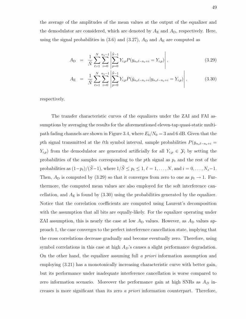
49
the average of the amplitudes of the mean values at the output of the equalizer and
the demodulator are considered, which are denoted by AE and AD, respectively. Here,
using the signal probabilities in (3.6) and (3.27), AD and AE are computed as
AD =1
N
N∑
`=1
ns−1∑
i=0
∣∣∣∣∣∣
S−1∑
p=0
Yi,pP (yns`−ns+i = Yi,p)
∣∣∣∣∣∣
, (3.29)
AE =1
N
N∑
`=1
ns−1∑
i=0
∣∣∣∣∣∣
S−1∑
p=0
Yi,pP (yns`−ns+i|yns`−ns+i = Yi,p)
∣∣∣∣∣∣
, (3.30)
respectively.
The transfer characteristic curves of the equalizers under the ZAI and FAI as-
sumptions by averaging the results for the aforementioned eleven-tap quasi-static multi-
path fading channels are shown in Figure 3.4, where Eb/N0 = 3 and 6 dB. Given that the
pth signal transmitted at the `th symbol interval, sample probabilities P (yns`−ns+i =
Yi,p) from the demodulator are generated artificially for all Yi,p ∈ Yi by setting the
probabilities of the samples corresponding to the pth signal as pt and the rest of the
probabilities as (1−pt)/(S−1), where 1/S ≤ pt ≤ 1, ` = 1, . . . , N , and i = 0, . . . , Ns−1.
Then, AD is computed by (3.29) so that it converges from zero to one as pt → 1. Fur-
thermore, the computed mean values are also employed for the soft interference can-
cellation, and AE is found by (3.30) using the probabilities generated by the equalizer.
Notice that the correlation coefficients are computed using Laurent’s decomposition
with the assumption that all bits are equally-likely. For the equalizer operating under
ZAI assumption, this is nearly the case at low AD values. However, as AD values ap-
proach 1, the case converges to the perfect interference cancellation state, implying that
the cross correlations decrease gradually and become eventually zero. Therefore, using
symbol correlations in this case at high AD’s causes a slight performance degradation.
On the other hand, the equalizer assuming full a priori information assumption and
employing (3.21) has a monotonically increasing characteristic curve with better gain,
but its performance under inadequate interference cancellation is worse compared to
zero information scenario. Moreover the performance gain at high SNRs as AD in-
creases is more significant than its zero a priori information counterpart. Therefore,

50
a feasible hybrid strategy for best achievable performance is to employ the former
equalizer initially, and then to switch to the latter one as the a priori information to
0 0.2 0.4 0.6 0.8 10
0.1
0.2
0.3
0.4
0.5
0.6
AD
AE
TE, ZAI
TE, FAI
TD→E −1 , I
Dec=0
TD→E −1 , I
Dec=0.35
TD→E −1 , I
Dec=1
Simulatedtrajectoryfor I
Dec=0
Simulatedtrajectory
for IDec
=0.35
Simulatedtrajectoryfor I
Dec=1
Figure 3.5. Comparison of the simulated trajectories and the characteristic curves for
the TDE and the demodulator at Eb/N0=3 dB
the equalizer is improved. In Figure 3.5, the simulated trajectories at Eb/N0 = 3 dB
between the equalizer and the demodulator are illustrated for three different sets of a
priori knowledge from the decoder, where the equalizer coefficients are set as (3.21)
for AD values less than 0.4 and as (3.20) for greater values. As proposed in [46], the
LLRs {La(um)} are generated according to the single-parameter Gaussian model in
(2.68) and IDec values are computed as the mutual information between the encoded
bits and the LLRs as in (2.70), by using the conditional PDFs in (2.69) belonging
to this model. In Figure 3.5, simulated trajectories tend to follow the path confined
between the equalizer and demodulator characteristic curves so that the simulated and
semi-analytical results are almost consistent. The transfer characteristic curves for the
equalizer are obtained as in Figure 3.4, where the demodulator characteristic curves
are found by generating the equalizer outputs artificially. For this purpose, the model

51
for the equalizer output in (3.14) is considered as
cn = fH rn := fHHe cn + fHdn, (3.31)
where dn, defined similar to the channel noise vector vn in (3.9) as,
dn =[
dn+F dn+F−1 . . . dn−B+1 dn−B
]T
(3.32)
contains the i.i.d. additive Gaussian noise terms each with zero-mean and variance σ2d.
Because channel noise terms after low-pass filtering and sampling are assumed to be
white at the beginning of this section, the elements of dn are also generated as white
Gaussian random variables. Note that each di (i = n + F, . . . , n − B) contains the
corresponding channel noise sample vi as well as the uncancelled interference for the
symbol cn. Therefore it is assumed that σ2v ≤ σ2
d where the equality holds in the case
of perfect interference cancellation. Here Dmin in (3.30) corresponds to the average
squared distance where the parameters for the model in (3.31) are set as σ2d = σ2
v
and f = fFAI. Then the equalizer output at each time instant is artificially generated
by (3.31), and the symbol probabilities are computed using (3.24), (3.25), and (3.27).
Afterwards, these probabilities are fed to the demodulator. Using the same switching
condition considered to obtain the simulated trajectories, the discrete-time symbols
that give AE values (computed by (3.30)) from zero to the output of the equalizer’s
characteristic curve for AD = 0.4 under no a priori information assumption are found
by employing (3.20) in (3.31), where the symbols that result in greater AE values are
generated by inserting (3.21) into (3.31) so that AE converges to one as σ2d approaches
σ2v . As shown in Figure 3.5, it is not possible to improve the equalizer outputs for
AD < 0.4 due to the lower gain of the equalization method using (3.20). Moreover,
for larger AD values, it is observed that the equalizer outputs are getting worse after
several equalizer/demodulator iterations (see the trajectory for IDec = 0.35). This is
because the equalizer outputs are correlated, and deinterleaving is not possible since
the interleaving after the CPM modulation destroys the phase continuity [8]. There-
fore, it is more convenient to enhance the a priori information from the demodulator
to get better equalizer outputs by performing a couple of demodulator/decoder itera-

52
tions (which improve IDec), instead of employing more than one equalizer/demodulator
iteration with the same IDec.
In case of back-end iterations, the demodulator transforms the a priori infor-
mation {La(um)} for the interleaved code bits from the channel decoder to {Le(um)},given the tilted-phase CPM signal probabilities from the equalizer. LLRs {La(um)} are
Figure 3.6. EXIT chart analysis for the back-end iterations of the doubly-iterative
receiver with TDE
generated depending on the model in (2.68), and IDec values are computed as in (2.70)
using the conditional PDFs in (2.69) belonging to this model, as previously stated. Af-
ter the output conditional PDFs are determined by histogram measurements, ID→ Dec
is computed in the same way, as the mutual information between the encoded bits
and the LLRs at the output of the demodulator [46]. Similar procedure is followed to
compute ID→ Dec and IDec at the input and output of the channel decoder, respectively.
The three-dimensional plot in Figure 3.6 illustrates the EXIT behavior for eleven-tap
quasi-static channels at Eb/N0 = 3 dB between the demodulator (upper surface) and
the decoder for varying information from the equalizer. The tilted-phase CPM sig-
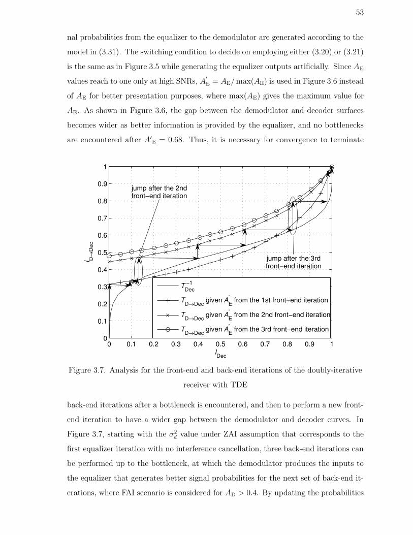
53
nal probabilities from the equalizer to the demodulator are generated according to the
model in (3.31). The switching condition to decide on employing either (3.20) or (3.21)
is the same as in Figure 3.5 while generating the equalizer outputs artificially. Since AE
values reach to one only at high SNRs, A′E = AE/ max(AE) is used in Figure 3.6 instead
of AE for better presentation purposes, where max(AE) gives the maximum value for
AE. As shown in Figure 3.6, the gap between the demodulator and decoder surfaces
becomes wider as better information is provided by the equalizer, and no bottlenecks
are encountered after A′E = 0.68. Thus, it is necessary for convergence to terminate
0 0.1 0.2 0.3 0.4 0.5 0.6 0.7 0.8 0.9 10
0.1
0.2
0.3
0.4
0.5
0.6
0.7
0.8
0.9
1
IDec
I D→
Dec
TDec −1
TD→Dec
given AE’ from the 1st front−end iteration
TD→Dec
given AE’ from the 2nd front−end iteration
TD→Dec
given AE’ from the 3rd front−end iteration
jump after the 2ndfront−end iteration
jump after the 3rdfront−end iteration
Figure 3.7. Analysis for the front-end and back-end iterations of the doubly-iterative
receiver with TDE
back-end iterations after a bottleneck is encountered, and then to perform a new front-
end iteration to have a wider gap between the demodulator and decoder curves. In
Figure 3.7, starting with the σ2d value under ZAI assumption that corresponds to the
first equalizer iteration with no interference cancellation, three back-end iterations can
be performed up to the bottleneck, at which the demodulator produces the inputs to
the equalizer that generates better signal probabilities for the next set of back-end it-
erations, where FAI scenario is considered for AD > 0.4. By updating the probabilities

54
from the equalizer following each set of back-end iterations, the convergence is achieved
after three front-end iterations.
3.3. Simulation Results
In this section, the BER performance of the doubly-iterative receiver with TDE
is presented for different number of front- and back-end iterations. Moreover, the BER
performance of the proposed receiver is compared to that of the TAE and the case
without ISI, as well. As decribed at the beginning of this chapter, in TAE imple-
mentation, soft information is exchanged between the optimal CED and the channel
decoder where both modules apply the Log-BCJR algorithm. The parameters used
in the BER simulations are selected as those in the EXIT chart analysis so that bi-
nary 3RC CPM with L = 3 and h = 0.5 is considered. Before applying CPM, bits
are encoded by rate-1/2 convolutional code with generator polynomial (64, 74)8. Each
data packet consists of 256 bits. Random interleaving is applied since it results in high
performance as shown in [8]. The channel resolution is Ts = T/2, number of samples
per symbol period is ns = 2, and the two-sided bandwidth of the low-pass filter is
2/T so that more than 99.9 percent of the signal energy is recovered [2]. The static
ISI channel is selected as Proakis’ A [66] with channel tap weights [0.04 -0.05 0.07
-0.21 -0.5 0.72 0.36 0.00 0.21 0.03 0.07]. The filter parameters are set as F = 11 and
B = 10 which lead to Lf = 22. The channel coefficients are normalized to have unit
total energy. The BER performance is also observed in case of eleven-tap quasi-static
multipath fading channels (channel I) changing independently at each packet trans-
mission. The channel coefficients are generated as complex Gaussian random variables
with exponentially decaying power profile. Here, hl as the lth path gain is a zero-mean
complex Gaussian random variable with variance being equal to e−l/2/( ∑10
m=0 e−m/2)
and the corresponding path delay is lTl where l = 0, 1, . . . , 10. Furthermore, the six-tap
typical urban channel (channel II) model in [22] is considered, where the variances of
the complex Gaussian path coefficients are [0.189 0.379 0.255 0.090 0.055 0.032] and
the corresponding path delays are [0 Ts 2Ts 8Ts 12Ts 25Ts]. In the legends of the fig-
ures for the BER performance, the abbreviations FIT and BIT are used to denote the
front-end iterations and the back-end iterations, respectively. For instance, “4th FIT

55
w/ 3 BIT” denotes the fourth execution of one SIC/TDE iteration followed by three
demodulator/decoder iterations at the back-end. In consistency with Section 3.2, AD
2 4 6 8 10 12 14 16 18 20 2210−7
10−6
10−5
10−4
10−3
10−2
10−1
100
Eb/N
0 (dB)
BER
no ISI (12 iterations)TAE, Proakis’ A (12 iterations)turbo TDE, Proakis’ A (12 FIT w/ 1 BIT)TAE, channel I (12 iterations)turbo TDE, channel I (12 FIT w/ 1 BIT)
1st iteration
12th iteration
12th FIT with 1 BIT
1st FIT w/ 1 BIT
Figure 3.8. BER performance for no ISI, Proakis’ A channel, and channel I
is computed as in (3.29) before each equalizer iteration, and (3.20) is replaced with
(3.21) for AD values greater than 0.4.
The BER performance of the proposed receiver and TAE in Proakis’ A channel
and eleven-tap quasi-static channels, and the iterative demodulation and decoding in
AWGN channel are presented in Figure 3.8. When the ISI channel is not present,
the receiver consists of a CPM demodulator followed by the channel decoder. Both
the demodulator and the channel decoder employ the Log-BCJR algorithm. Twelve
iterations are run for the turbo CPM demodulation and channel decoding. For doubly-
iterative equalization, twelve executions of one FIT followed by one BIT are performed.
The TAE performs twelve iterations between CED and the channel decoder. Due to
the suboptimality of the proposed receiver, the BER for the first front-end + back-end
iteration is below 10−5 only after 21 dB, for Proakis’ A channel. Thus, after twelve
passes of one FIT with one BIT, performance gain is about 15 dB. As shown in Figure

56
3.8, performance of the proposed receiver is very close to that of TAE in Proakis’ A
channel.
The receiver may encounter bottlenecks on convergence without performing more
6 8 10 12 14 16 18 20 2210−7
10−6
10−5
10−4
10−3
10−2
10−1
100
Eb/N
0 (dB)
BE
R
1 FIT w/ 12 BIT (channel I)3 FIT w/ 4 BIT (channel I)12 FIT w/ 1 BIT (channel I)1 FIT w/ 12 BIT (channel II)3 FIT w/ 4 BIT (channel II)12 FIT w/ 1 BIT (channel II)
Figure 3.9. BER performance in channels I and II
than one front-end equalizer iteration, as also observed in Section 3.2. This behavior
can be observed in Figure 3.9, as well. Here, by performing twelve passes of one
front-end iteration followed by one back-end iteration, BER values below 10−5 are
observed after 21 dB and 18 dB in channel I channel II scenarios, respectively, where
the performance gain compared to performing only one front-end iteration followed
by twelve back-end iterations is around 0.7 dB and 1 dB respectively. However, it
is not always necessary to employ many equalizer iterations since running sufficient
number of back-end iterations improves the a priori information for SIC and reduces
the number of the front-end iterations. In Figure 3.9, by employing four front-end
iterations, where each is followed by three back-end iterations, similar performance
is observed compared to twelve passes of one front-end iteration with one back-end

57
iteration, where the number of equalizer iterations is three times less in the former
scenario.

58
4. DOUBLE TURBO EQUALIZATION OF CPM WITH
FREQUENCY DOMAIN PROCESSING
In order to alleviate the high complexity of the CED module in [10] which uses a
single super trellis for the optimal detection of CPM over the multipath fading chan-
nels and motivated by the near-optimum error performance of the iterative receivers,
an alternative CPM receiver is proposed in Chapter 3 where the equalization, CPM
demodulation, and channel decoding operations are assigned to three separate SISO
blocks and the central demodulator is coupled with both the front-end equalizer and
the back-end decoder in a doubly-iterative architecture. The most important feature
of this receiver is that a soft-information-aided MMSE TDE is used at its front-end
instead of a trellis-based algorithm, which presents a low complexity alternative while
still achieving a performance close to the “no interference” bound. Notice that comput-
ing the MMSE TDE coefficients requires some cumbersome matrix inversions causing
the computational load to be still relatively large in long channel responses. As pre-
sented in [19]-[21], by doing the equalization in the frequency domain the complexity
can be reduced further while attaining the same and often better performance.
The FDE approach has also been extended to the equalization of CPM in [22],
where the FDE is not equipped with any SISO capability and thus is not suitable
for turbo processing. The advantages of frequency-domain processing and iterative
information exchange are combined in [23], where a SISO BFDE is followed by the SISO
CPM demodulator and channel decoder modules in the proposed TLE structure. Here,
the soft CPM signal information to start the subsequent equalization iterations are
computed from the code bit probabilities obtained from the back-end channel decoder.
However, this produces long error bursts due to the inherent modulation memory and
thus, the CPM signal probabilities are delivered to BFDE only at certain epoches
to break up the error propagation at the expense of obtaining only a slight turbo
gain. Moreover, because the proposed FDE operates on blocks of information, it still
involves matrix inversions which result in an increased computational cost. For this

59
reason, herein a soft-information-aided FDE for CPM is proposed which overcomes the
disadvantages of that in [23] and replaces the front-end TDE in Figure 3.2, so as to
achieve a better error performance with lower computational complexity compared to
the methods in both Chapter 3 and [23] .
In the proposed receiver, the frequency-domain processing of CPM signals is
made possible by inserting a cyclic guard interval longer than the channel memory
while maintaining the phase continuity of CPM. The FDE is equipped with an a
priori SIC and an APP mapper to generate soft information for the central CPM
demodulator. As described in Chapter 3, the decoder used for demodulation computes
extrinsic information at its output on both the discrete-time CPM signals and the
coded bits. Then, these two soft outputs are employed in a doubly-iterative information
exchange where the CPM demodulator is coupled with both the front-end FDE and
the back-end decoder. Because the CPM signal probabilities are not computed from
the code bit probabilities, the error bursts of [23] due to the modulation memory are
not encountered, which results in a significant performance improvement. Moreover,
because its implementation does not involve any matrix inversion, the proposed SISO
FDE is computationally less complex than the linear equalizers in Chapter 3 and [23].
The doubly-iterative CPM receiver with the FDE is also more feasible compared to the
TLE in [23] in attaining faster convergence to low BERs because the number of front-
end iterations are decreased by performing several demodulation/decoding iterations
per each equalization iteration to improve the equalizer a priori information. This
behavior can be justified by two and three dimensional EXIT charts analysis similar
to the approach in Section 3.2 presented for the doubly-iterative receiver with TDE.
The rest of the chapter is organized as follows. In Section 4.1, the cyclic guard
insertion, the doubly-iterative receiver with FDE, the proposed soft-information-aided
FDE algorithm, and the complexity comparisons with alternative receiver structures
are presented. A similar comparison in terms of BER simulations is given in Section
4.3 after the convergence analysis in Section 4.2.

60
4.1. Doubly-Iterative Equalization with Frequency Domain Processing
At the transmitter, a length-Lb data bit sequence with elements bi ∈ {0, 1},i = 1, . . . , Ld, is encoded by a rate-Lb/Lu convolutional code to form um ∈ {−1, +1}where m = 1, . . . , Lu. Then um are interleaved to um, which are mapped onto the
M -ary symbols x` defined in Section 2.1.1 where ` = 1, . . . , N with N = Lu/ log2 M .
Using these symbols, CPM waveforms are generated and transmitted throughout the
multipath fading channel. The receiver observes a noisy linear convolution of the
transmitted signals with the multipath fading channel. To make frequency-domain
processing possible , the transmitter structure in Figure 3.1 needs to be modified by
deploying a new module in between the symbol mapper and the CPE to append a cyclic
prefix to the transmitted signal sequence at the expense of an increased redundancy.
Here the length of the cyclic prefix, G, is chosen as the minimum number of symbol
{x`
}0−G+1
={x`
}NN−G+1
{x`
}N−G−le1 =
{x`
}N−G−le1
{x`
}N−ltN−G+1
={x`
}N−ltN−G+1
Cyclicprefix
Datasymbols
le tailsymbols
Datasymbols
lt tailsymbols
Figure 4.1. Modulating sequence with the cyclic prefix
periods to avoid interblock interference due to the multipath channel effects. However,
the transmission of CPM signals also requires the preservation of phase continuity
within each transmitted block and between consecutive transmitted blocks. Observing
the similarity of the CPE to a recursive convolutional encoder, this phase continuity
can be attained by inserting two sets of tail symbols of lengths le and lt after the
first N − G + lt modulating symbols and to the end of the whole symbol sequence,
respectively. After setting the initial state for the CPE trellis as the zero state in
(2.19) before applying the modulating symbol sequence, by choosing lt as the minimum
number of symbols to return to the zero state from any trellis state and le ≥ lt as the
number of symbols to return to and stay at the zero state, it is assured that the CPE
trellis path returns to the zero state at n = N − G + lt + le and n = N + lt + le. The
symbol sequence with tail symbols becomes {x`}N1 where N = N + lt + le. Then, the
length-G cyclic prefix, selected as the last G symbols, is appended to the beginning

61
of the symbol block as depicted in Figure 4.1 and the new symbol sequence becomes
x` = x(`−1)N+1, ` = −G + 1, . . . ,−1, 0, 1, . . . , N , where (·)N stands for the modulo-N
operation. The CPE employs the new symbol sequence xN−G+1 = {x`}N
−G+1 to generate
the tilted-phase signal y(t, xN−G+1) so that y(t, xN
−G+1)= y(t+NT, xN−G+1) on the interval
−GT < t < 0. By compensating for the frequency shift in (2.14), the CPM signal is
obtained as
c(t, xN−G+1) = y(t, xN
−G+1)e−jπh(M−1)t/T , −GT < t < NT. (4.1)
Note that this new sequence ensures that the CPE trellis path for each packet begins
and ends at the zero state and therefore no phase discontinuities are encountered during
the transitions between consecutive packets. Furthermore, within each packet, the
trellis path returns to the zero state after the first G symbols so that the cyclic guard
interval does not disrupt the phase continuity. When le is chosen properly such that
hN is an even integer, (4.1) yields that c(t, xN−G+1) = c(t + NT, xN
−G+1) on the interval
−GT < t < 0 since e−jπh(M−1)(t+NT )/T = e−jπh(M−1)t/T .
After the transmission through the ISI channel, the received signal at the base-
band using the similar representation in (2.25) is denoted as
r(t) =Lc−1∑
l=0
hlc(t − lTs, xN−G+1) + v(t), −GT < t < NT, (4.2)
where v(t) is the zero-mean AWGN term. After the removal of the prefix and low-pass
filtering with a two-sided bandwidth of 1/Ts Hertz, the discrete symbols are obtained
by sampling the filter output every Ts seconds such that the additive noise is still white
and there is no aliasing. After sampling, (4.2) becomes
r(nTs) =Lc−1∑
`=0
h`c(nTs − `Ts, xN−G+1) + v(nTs), n = 0, . . . , N − 1, (4.3)
where N = nsN . Then, defining rn := r(nTs), cn := c(nTs, xN−G+1), vn := v(nTs),
hN−10 := {hn}N−1
0 that is obtained through zero padding after the first Lc terms, and
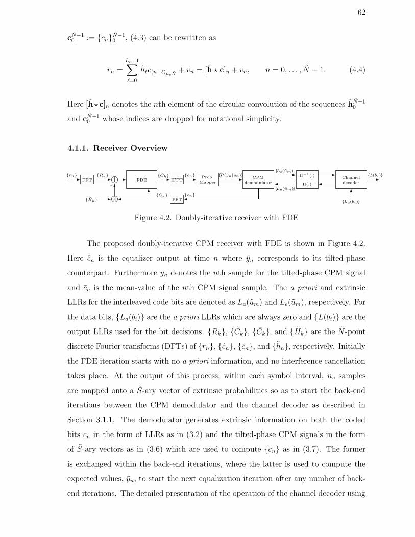
62
cN−10 := {cn}N−1
0 , (4.3) can be rewritten as
rn =Lc−1∑
`=0
h`c(n−`)nsN+ vn = [h ? c]n + vn, n = 0, . . . , N − 1. (4.4)
Here [h?c]n denotes the nth element of the circular convolution of the sequences hN−10
and cN−10 whose indices are dropped for notational simplicity.
4.1.1. Receiver Overview
FFT FDE IFFTProb.
MapperCPM
demodulator
Π−1(.)
Π(.)
Channeldecoder
FFT
{rn} {Rk}+
-
{cn} {P (yn|yn)}{Le(um)}
{La(um)}
{La(bi)}
{L(bi)}
{cn}{Ck}
{Ck}
{Hk}
Figure 4.2. Doubly-iterative receiver with FDE
The proposed doubly-iterative CPM receiver with FDE is shown in Figure 4.2.
Here cn is the equalizer output at time n where yn corresponds to its tilted-phase
counterpart. Furthermore yn denotes the nth sample for the tilted-phase CPM signal
and cn is the mean-value of the nth CPM signal sample. The a priori and extrinsic
LLRs for the interleaved code bits are denoted as La(um) and Le(um), respectively. For
the data bits, {La(bi)} are the a priori LLRs which are always zero and {L(bi)} are the
output LLRs used for the bit decisions. {Rk}, {Ck}, {Ck}, and {Hk} are the N -point
discrete Fourier transforms (DFTs) of {rn}, {cn}, {cn}, and {hn}, respectively. Initially
the FDE iteration starts with no a priori information, and no interference cancellation
takes place. At the output of this process, within each symbol interval, ns samples
are mapped onto a S-ary vector of extrinsic probabilities so as to start the back-end
iterations between the CPM demodulator and the channel decoder as described in
Section 3.1.1. The demodulator generates extrinsic information on both the coded
bits cn in the form of LLRs as in (3.2) and the tilted-phase CPM signals in the form
of S-ary vectors as in (3.6) which are used to compute {cn} as in (3.7). The former
is exchanged within the back-end iterations, where the latter is used to compute the
expected values, yn, to start the next equalization iteration after any number of back-
end iterations. The detailed presentation of the operation of the channel decoder using
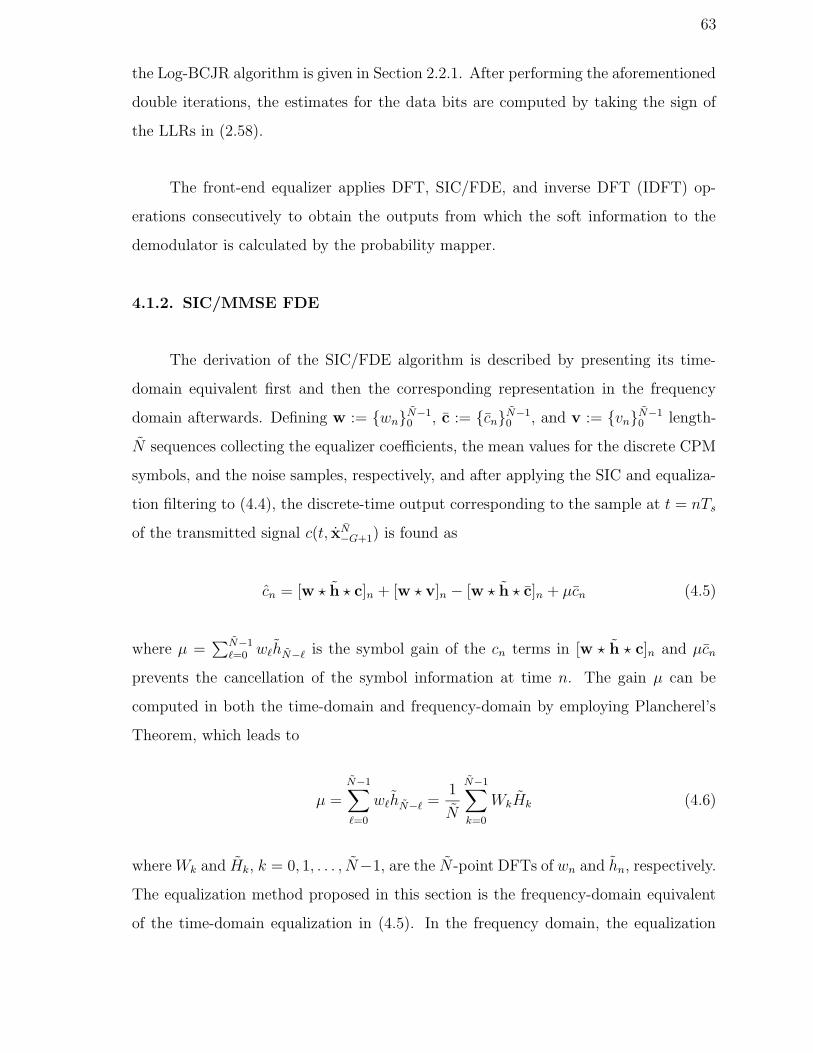
63
the Log-BCJR algorithm is given in Section 2.2.1. After performing the aforementioned
double iterations, the estimates for the data bits are computed by taking the sign of
the LLRs in (2.58).
The front-end equalizer applies DFT, SIC/FDE, and inverse DFT (IDFT) op-
erations consecutively to obtain the outputs from which the soft information to the
demodulator is calculated by the probability mapper.
4.1.2. SIC/MMSE FDE
The derivation of the SIC/FDE algorithm is described by presenting its time-
domain equivalent first and then the corresponding representation in the frequency
domain afterwards. Defining w := {wn}N−10 , c := {cn}N−1
0 , and v := {vn}N−10 length-
N sequences collecting the equalizer coefficients, the mean values for the discrete CPM
symbols, and the noise samples, respectively, and after applying the SIC and equaliza-
tion filtering to (4.4), the discrete-time output corresponding to the sample at t = nTs
of the transmitted signal c(t, xN−G+1) is found as
cn = [w ? h ? c]n + [w ? v]n − [w ? h ? c]n + µcn (4.5)
where µ =∑N−1
`=0 w`hN−` is the symbol gain of the cn terms in [w ? h ? c]n and µcn
prevents the cancellation of the symbol information at time n. The gain µ can be
computed in both the time-domain and frequency-domain by employing Plancherel’s
Theorem, which leads to
µ =N−1∑
`=0
w`hN−` =1
N
N−1∑
k=0
WkHk (4.6)
where Wk and Hk, k = 0, 1, . . . , N−1, are the N -point DFTs of wn and hn, respectively.
The equalization method proposed in this section is the frequency-domain equivalent
of the time-domain equalization in (4.5). In the frequency domain, the equalization
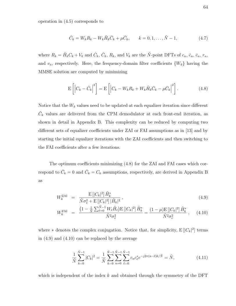
64
operation in (4.5) corresponds to
Ck = WkRk − WkHkCk + µCk, k = 0, 1, . . . , N − 1, (4.7)
where Rk = HkCk + Vk and Ck, Ck, Rk, and Vk are the N -point DFTs of cn, cn, cn, rn,
and vn, respectively. Here, the frequency-domain filter coefficients {Wk} having the
MMSE solution are computed by minimizing
E
[∣∣∣Ck − Ck
∣∣∣
2]
= E
[∣∣∣Ck − WkRk + WkHkCk − µCk
∣∣∣
2]
. (4.8)
Notice that the Wk values need to be updated at each equalizer iteration since different
Ck values are delivered from the CPM demodulator at each front-end iteration, as
shown in detail in Appendix B. This complexity can be reduced by computing two
different sets of equalizer coefficients under ZAI or FAI assumptions as in [13] and by
starting the initial equalizer iterations with the ZAI coefficients and then switching to
the FAI coefficients after a few iterations.
The optimum coefficients minimizing (4.8) for the ZAI and FAI cases which cor-
respond to Ck = 0 and Ck = Ck assumptions, respectively, are derived in Appendix B
as
W ZAIk =
E [|Ck|2] H∗k
Nσ2v + E [|Ck|2] |Hk|2
, (4.9)
WFAIk =
(1 − 1
N
∑N−1`=0 W`H`
)E [|Ck|2] H∗
k
N2σ2v
=(1 − µ)E [|Ck|2] H∗
k
N2σ2v
, (4.10)
where ∗ denotes the complex conjugation. Notice that, for simplicity, E [|Ck|2] terms
in (4.9) and (4.10) can be replaced by the average
1
N
N−1∑
k=0
|Ck|2 =1
N
N−1∑
k=0
N−1∑
n=0
N−1∑
`=0
cnc∗`e
−j2π(n−`)k/N = N , (4.11)
which is independent of the index k and obtained through the symmetry of the DFT

65
operation and the unit-amplitude CPM signals. Then, using this replacement and the
joint solution of (4.6) and (4.10) for µ together, the equalizer coefficients in (4.9) and
(4.10) for the ZAI and FAI cases simplify to
W ZAIk =
H∗k
σ2v + |Hk|2
, (4.12)
WFAIk =
H∗k
Nσ2v + (1/N)
∑N−1`=0 |H`|2
, (4.13)
respectively.
The SIC exploits the mean values, {cn}, which are calculated by the demodulator
as shown in (3.7). After performing the DFT operations on (3.7) and (4.4), and
computing the frequency-domain outputs with (4.7) by either using (4.12) or (4.13),
the time-domain outputs, {cn}, are found by the IDFT operation. Then, the soft
information for CPM demodulator is computed by the probability mapper. For this
purpose, the equalizer output with the tilted-phase is found as yn = cnejπh(M−1)n/ns , n =
0, 1, . . . , N − 1, which can be viewed as yn = µyn + υn as in (3.23) where µ is the
symbol gain presented in (4.6) and υn is the zero-mean complex additive Gaussian
noise [13, 15]. The probability mapper calculates the sample probabilities delivered to
the demodulator as
P (yns`−ns+i|yns`−ns+i = Yi,p) =e−
|yn−µYi,p|2
σ2
∑S−1m=0 e−
|yn−µYi,m|2
σ2
(4.14)
for ` = 1, . . . , N , i = 0, 1, . . . , ns − 1, p = 0, 1, . . . , S − 1, and Yi,p ∈ Yi as described
in Section 2.1.1, where σ2 is the average variance for υn computed at each equalizer
iteration as in (3.26) using the symbol gain in (4.6) and the FDE outputs.
4.1.3. Complexity Comparison
The SIC/FDE employs fast Fourier transform (FFT) and inverse FFT (IFFT)
operations. Considering that N is an integer power of two, FFT or IFFT requires

66
N log2 N complex multiplications and approximately those many complex additions
[67]. Thus, the number of real multiplications and the real additions (approximately)
to obtain all Rk and Ck values is equal to 8N log2 N , by assuming that the mean values
cn from the CPM decoder are available. Then, given Wk, Hk, and µ, (4.7) leads to 8N
real multiplications and 6N real additions, and the time-domain symbol estimates are
obtained after 4N log2 N real multiplications and additions. Thus, the total number
of real multiplications and additions per SIC/equalizer iteration are 12N log2 N + 8N
and approximately 12N log2 N + 6N , respectively. Moreover, at the initial equaliza-
tion iteration, Hk values are computed by at most 4N log2 N real multiplications and
additions, whereas the computation of Wk and µ for the ZAI and FAI scenarios require
10N + 4 real multiplications and 5N real additions.
Table 4.1. Complexity of the SISO Modules Used by the Proposed Receiver, the
Receivers in Chapter 3 and [23], and TAEFDE TDE BFDE [23] CED [10] CPM Channel
Demodulator Decoder
Real O(U)+ O(L3f )+ O(niU3)+ O(niUPML+Mc−1) O(niUPML) O(niU2lc+1)
multiplications O(niU log2 U)+ O(niULf )+ O(niUPML)
and additions O(niUPML) O(niUPML)
U , ni, Lf , Mc, L, M , P, and lc denote the block length, number of iterations, length of the TDE filter, length of the
multipath channel in terms of symbol intervals, memory length of CPM, modulation order, denominator of the modulation index,
and the memory length of the convolutional code, respectively.
The approximate computational complexity for the proposed FDE is presented
in Table 4.1, along with the TDE proposed in Chapter 3, the BFDE in [23] and the
optimal CED in [10] using the Log-BCJR algorithm. Also included in the table are the
complexities of the SISO CPM demodulator and the channel decoder so that the com-
plexity comparisons of different turbo architectures using these blocks can be obtained.
Here ni, Mc = bLc/nsc + 1, lc, and Lf denote the number of iterations, length of the
multipath channel in terms of symbol intervals with b.c being the floor operator, the
memory length of the convolutional code, and the length of the TDE filters in (3.20)
and (3.21) which depend on Lc linearly, respectively. The example below presents the
approximate number of real multiplications and additions required throughout a signal
block for the proposed turbo receiver with FDE (turbo FDE) in Figure 4.2, the turbo
receiver with TDE (turbo TDE) in Figure 3.2 replacing the front-end FDE in Figure

67
4.2 by the SISO TDE filter introduced in Section 3.1.2, the TLE in [23] in which the
BFDE is followed by the CPM demodulator and the channel decoder modules, and
the aforementioned TAE which exchanges soft information between the optimal CED
module and the channel decoder where both SISO modules employ the Log-BCJR
algorithm.
Example: It is assumed that Ld = 126 data bits are encoded by a rate-1/2
convolutional code so that Lb = 252 code bits are obtained, where the memory length
of the convolutional code is lc = 3. The parameters for the CPM scheme is M = 2,
L = 3 and h = 0.5 with P = 2. To apply the proposed turbo FDE and the TLE in
[23], a cyclic guard interval is added to the transmitted block. For this purpose, four
tail symbols are inserted as shown in Figure 4.1 where le = 2 and lt = 2, and the
length of the modulating sequence is N = 256. The turbo receivers with time-domain
equalization methods in Chapter 3 and [10] do not require tail symbols and cyclic guard
addition so that the length of the modulating sequence is N = 252. For the multipath
fading channel, it is assumed that Lc = 11, the channel resolution is Ts = T/2 with
Table 4.2. Computational Complexity per Signal Block for the Proposed Receiver,
the Turbo Equalizers in Chapter 3 and [23], and TAEReceiver Computational Complexity
Turbo FDE with nf front-end O(nsN) + O(nf nsN log2 nsN) + O(nf nsNPML) + O(niLbPML) + O(niLb2lc+1)
and ni back-end iterations
Turbo TDE with nf front-end O(L3f ) + O(nf nsNLf ) + O(nf nsNPML) + O(niLbPML) + O(niLb2lc+1)
and ni back-end iterations
TLE [23] with ni O(nin3sN3) + O(ninsNPML) + O(niLbPML) + O(niLb2lc+1)
iterations
TAE with ni O(niNPML+Mc−1) + O(niLb2lc+1)
iterations
N , N , ns, Lf , Mc, L, M , P, and lc denote the length of the modulation sequence, length of the modulation sequence with
tail symbols, number of samples per symbol period, length of the TDE filter, length of the multipath channel in terms of
symbol intervals, memory length of CPM, modulation order, denominator of the modulation index, and the memory length of
the convolutional code, respectively.
ns = 2, and, therefore, the maximum tap delay is 5T . After the addition of the cyclic
guard interval, the duration of the transmitted packet is 261T with G = 5. Thus, the
number of extra tail and guard symbols employed by the frequency-domain methods
is only le + lt + G = 9 compared to the time-domain methods. The computational
load for the aforementioned turbo receivers are presented in Table 4.2 by using the
approximate complexity values in Table 4.1 for the SISO modules deployed by these

68
receivers. At the first and second rows of Table 4.2, the complexity values for the turbo
FDE and turbo TDE are given, respectively. Using the doubly-iterative structure of
these receivers, each of the nf FITs is followed by ni/nf BITs so that ni BITs are
performed in total. As in Section 3.3, the TDE filter length is Lf = 2Lc. Because
the TLE and TAE cannot perform double iterations, all the SISO modules at these
receivers are employed throughout ni iterations, as presented at the third and fourth
rows of Table 4.2, respectively. The number of iterations are set as nf = 4 and ni = 12,
which are same as the values used for the BER simulations in the present chapter and
Section 3.3.
By using the aforementioned parameter values in Table 4.2, it is observed that
the number of computations for the proposed turbo FDE at the first row is fewer than
the ones for the turbo TDE at the second row, respectively, by adding only nine extra
symbols to the transmitted packet. This is because of the cube complexity that comes
from the matrix inversion operation in (3.20) and (3.21) for TDE and the dependency of
the filter length Lf on the channel length Lc. Note that the redundancy for turbo FDE
to add the cyclic prefix increases linearly in longer channel impulse responses without
any computational change whereas the turbo TDE encounters higher cube complexity.
The complexity of TLE does not depend on the length of the channel impulse response.
However it is computationally more demanding compared to the proposed turbo FDE
as shown at the third row of Table 4.2, depending on the matrix inversions required by
the BFDE at each iteration. Moreover, it is not possible to perform double iterations at
this receiver to reduce the complexity for equalization. Last row of Table 4.2 shows that
the TAE is also more complex compared to the proposed method. Here the complexity
of the optimal CED in [10] applied by TAE increases exponentially with the length
of the channel impulse response. For the proposed turbo FDE, the length of channel
impulse response does not have impact on the complexity in the expense of adding
redundancy which increases linearly with the channel memory length. Furthermore,
performance of the turbo FDE is better compared to the turbo TDE and TLE and is
close to that of TAE, as shown in Section 4.3.

69
4.2. EXIT Chart Analysis
Convergence behavior of the proposed doubly-iterative receiver with FDE is an-
alyzed using the same method in Section 3.2. The transfer characteristic functions for
the SISO modules in Figure 4.2 are shown in Figure 3.3. The method described in
Section 2.2.3 to obtain the transfer functions of the SISO decoders at a turbo receiver
depends on the availability of uncorrelated a priori information at the input of these
SISO modules and, therefore, requires the use of an interleaver between the corre-
sponding encoders at the transmitter. However, because interleaving after the CPM
modulation destroys the phase continuity, deinterleaving is not applicable between the
FDE and CPM demodulator in Figure 4.2. Therefore, the transfer characteristic curve
for the FDE is obtained by using the aforementioned average quantities in Section 3.2
which are computed as
AD =1
N
N∑
`=1
ns−1∑
i=0
∣∣∣∣∣∣
S−1∑
p=0
Yi,pP (yns`−ns+i = Yi,p)
∣∣∣∣∣∣
, (4.15)
AE =1
N
N∑
`=1
ns−1∑
i=0
∣∣∣∣∣∣
S−1∑
p=0
Yi,pP (yns`−ns+i|yns`−ns+i = Yi,p)
∣∣∣∣∣∣
. (4.16)
In (4.16), the probabilities in (4.14) are used where µ is the symbol gain in (4.6) and
{yn} are the tilted-phase equalizer outputs obtained from {cn} which correspond to
the N -point IDFT of the FDE outputs {Ck} in (4.7). AD and AE are used as the
information measures at the input and output of the equalizer. To obtain the equalizer
transfer characteristic curves, sample probabilities P (yns`−ns+i = Yi,p) in (3.6) from the
demodulator are generated artificially for all Yi,p ∈ Yi as described in Section 3.2 by
setting the probabilities of the samples corresponding to the pth signal as pt and the rest
of the probabilities as (1− pt)/(S − 1) given that the pth signal transmitted at the `th
symbol interval, where 1/S ≤ pt ≤ 1, ` = 1, . . . , N , and i = 0, . . . , Ns − 1. Then AD is
calculated in (4.15). Furthermore, the computed mean values are also employed for the
soft interference cancellation, and AE is found by (4.16) using the FDE outputs. The
FDE coefficients are set as (4.12)and (4.13) to obtain the transfer characteristic curves
for the zero and perfect a priori information scenarios, respectively, which are used

70
to determine the switching condition between these scenarios. For the demodulator
transfer characteristic curves, the FDE outputs in (4.7) are generated artificially as
Ck :=Ck
N
N−1∑
`=0
W`H` + WkDk, (4.17)
where {Ck} multiplied by the gain in (4.6) denote the N -point DFT of the signal
samples {cn}. The FDE coefficients in either (4.12) or (4.13) are used in (4.17) while
producing the equalizer outputs artificially. {Dk} are the N -point DFT of {dn} which
are defined similar to the channel noise samples {vn} in (4.4) as the i.i.d. additive
Gaussian noise terms each with zero-mean and variance σ2d. Because channel noise
terms after low-pass filtering and sampling are assumed to be white at the beginning of
this chapter, the elements of dn are also generated as white Gaussian random variables.
Note that each dn contains the corresponding channel noise sample vn as well as the
uncancelled interference for the symbol cn. Therefore it is assumed that σ2v ≤ σ2
d where
the equality holds in the case of perfect interference cancellation. The inputs {cn}to the probability mapper in Figure 4.2 are obtained by taking the N -point IDFT of
{Ck} generated using the model in (4.17), which are used to obtain the probabilities
in (4.14) to be delivered to the demodulator and to compute AE in (4.16).
As previously shown in Section 3.2, it is more effective in the doubly-iterative
architecture to perform back-end demodulator/decoder iterations after each equalizer
iteration to improve the demodulator outputs for the next equalizer iteration rather
than applying equalizer/demodulator iterations with constant information from the
channel decoder. At the back-end of the receiver, CPM demodulator and the channel
decoder exchange soft information for the encoded bits, and the convergence behav-
ior between these modules can be observed by using EXIT chart analysis. A two
dimensional graph as in [46] can be obtained by considering constant a priori infor-
mation from the equalizer to the demodulator.Moreover, a three dimensional graph as
in [47] can also be illustrated to observe the convergence behavior while the a priori
information from the equalizer improves. In this section, both graphs are obtained
by considering the mutual information between the encoded bits and the LLRs at the

71
output of the demodulator/decoder as described in Section 2.2.3.
In the convergence analysis (and in the BER simulations of the next section),
binary 3RC CPM scheme with L = 3 and h = 0.5 is considered, which employs
RC filtering with main lobe width of L symbol duration, as described in [2]. The
channel resolution is Ts = T/2, number of samples per symbol period is ns = 2, and
the two-sided bandwidth of the low-pass filter is 2/T so that more than 99.9 percent
of the signal energy is recovered [2]. A rate-1/2 convolutional code with generator
0 0.2 0.4 0.6 0.8 10
0.1
0.2
0.3
0.4
0.5
0.6
0.7
0.8
0.9
AD
AE
Eb/N
0=3 dB, ZAI
Eb/N
0=6 dB, ZAI
Eb/N
0=3 dB, FAI
Eb/N
0=6 dB, FAI
Figure 4.3. Transfer characteristic curves for the SIC/FDE at Eb/N0 = 3 and 6 dB
polynomial (64, 74)8 is used for channel coding [64]. For multipath fading, eleven-tap
quasi-static channels where the tap coefficients are zero-mean complex white Gaussian
random variables with exponentially decaying power profile are taken into account.
The variance of the lth path coefficient is e−l/2/( ∑10
m=0 e−m/2)
and the corresponding
path delay is lTs for l = 0, 1, . . . , 10. The complex channel noise is assumed AWGN
with zero mean and variance σ2v .
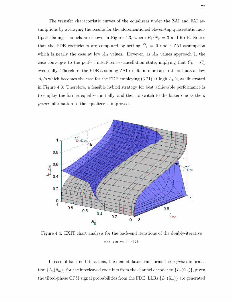
72
The transfer characteristic curves of the equalizers under the ZAI and FAI as-
sumptions by averaging the results for the aforementioned eleven-tap quasi-static mul-
tipath fading channels are shown in Figure 4.3, where Eb/N0 = 3 and 6 dB. Notice
that the FDE coefficients are computed by setting Ck = 0 under ZAI assumption
which is nearly the case at low AD values. However, as AD values approach 1, the
case converges to the perfect interference cancellation state, implying that Ck = Ck
eventually. Therefore, the FDE assuming ZAI results in more accurate outputs at low
AD’s which becomes the case for the FDE employing (3.21) at high AD’s, as illustrated
in Figure 4.3. Therefore, a feasible hybrid strategy for best achievable performance is
to employ the former equalizer initially, and then to switch to the latter one as the a
priori information to the equalizer is improved.
Figure 4.4. EXIT chart analysis for the back-end iterations of the doubly-iterative
receiver with FDE
In case of back-end iterations, the demodulator transforms the a priori informa-
tion {La(um)} for the interleaved code bits from the channel decoder to {Le(um)}, given
the tilted-phase CPM signal probabilities from the FDE. LLRs {La(um)} are generated

73
depending on the model in (2.68), and IDec values are computed as in (2.70) using the
conditional PDFs in (2.69) belonging to this model, as previously mentioned. After
the output conditional PDFs are determined by histogram measurements, ID→ Dec is
computed in the same way, as the mutual information between the encoded bits and
0 0.1 0.2 0.3 0.4 0.5 0.6 0.7 0.8 0.9 10
0.1
0.2
0.3
0.4
0.5
0.6
0.7
0.8
0.9
1
IDec
I D→
Dec
T −1Dec
TD→Dec
given AE’ from the 1st iteration
TD→Dec
given AE’ from the 2nd iteration
TD→Dec
given AE’ from the 3rd iteration
jump after the 2ndfront−end iteration
jump after the 3rdfront−end iteration
Figure 4.5. Analysis for the front-end and back-end iterations of the doubly-iterative
receiver with FDE
the LLRs at the output of the demodulator [46]. Similar procedure is followed to com-
pute ID→ Dec and IDec at the input and output of the channel decoder, respectively.
The three-dimensional plot in Figure 4.4 illustrates the EXIT behavior at Eb/N0 = 3
dB between the demodulator (upper surface) and the decoder for varying information
from the FDE. The tilted-phase CPM signal probabilities from the equalizer to the de-
modulator are computed by using the FDE outputs generated according to the model
in (4.17). The switching condition to decide on employing either (4.12) or (4.13) is
the same as in Figure 4.3 while generating the equalizer outputs artificially. Since
AE values reach to one only at high SNRs, A′E = AE/ max(AE) is used in Figure 4.4
instead of AE for better presentation purposes, where max(AE) gives the maximum
value for AE. As shown in Figure 4.4, the gap between the demodulator and decoder

74
surfaces becomes wider as better information is provided by the equalizer, and no
bottlenecks are encountered after AE = 0.6. Thus, it is necessary for convergence to
terminate back-end iterations after a bottleneck is encountered, and then to perform
a new front-end iteration to have a wider gap between the demodulator and decoder
curves. In Figure 4.5, starting with the σ2d value under zero information assumption
that corresponds to the first equalizer iteration with no interference cancellation, three
back-end iterations can be performed up to the bottleneck, at which the demodulator
produces the inputs to the equalizer that generates better signal probabilities for the
next set of back-end iterations, where FAI scenario is considered for AD > 0.3. By
updating the probabilities from the equalizer following each set of back-end iterations,
the convergence is achieved after four front-end iterations.
4.3. Simulation Results
In this section, the BER performance of the proposed turbo FDE is presented for
different number of front- and back-end iterations, and is also compared to those of the
TAE employing the CED in [10], the turbo TDE in Chapter 3, the TLE in [23], and
the performance in AWGN channel. The binary 3RC CPM with L = 3 and h = 0.5
is considered as in [2] with ns = 2, the two-sided bandwidth of the low-pass filter is
2/T , and the channel resolution is Ts = T/2, as in [23]. The rate-1/2 convolutional
code with generator polynomial (64, 74)8 is used, and random interleaving is applied.
First, the performance gap between the optimal and the proposed receiver is observed
in a mild Proakis’ A channel with coefficients [0.04 -0.05 0.07 -0.21 -0.5 0.72 0.36
0.00 0.21 0.03 0.07], where the delay of the mth path is mTs for m = 0, 1, . . . , 10.
The channel coefficients are normalized to have unit total energy. The aforementioned
receivers are also compared in a more severe eleven-tap quasi-static channel (channel I)
environment with deep spectral nulls, where the tap coefficients are zero-mean complex
white Gaussian random variables with exponentially decaying power profile such that
the variance of the mth path coefficient is e−m/2/( ∑10
l=0 e−l/2)
and the corresponding
path delay is mTs for m = 0, 1, . . . , 10. Furthermore, the six-tap typical urban channel
(channel II) model in [22] is considered, where the variances of the complex Gaussian
path coefficients are [0.189 0.379 0.255 0.090 0.055 0.032] and the corresponding path
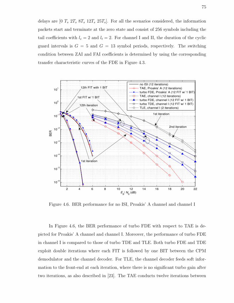
75
delays are [0 Ts 2Ts 8Ts 12Ts 25Ts]. For all the scenarios considered, the information
packets start and terminate at the zero state and consist of 256 symbols including the
tail coefficients with le = 2 and lt = 2. For channel I and II, the duration of the cyclic
guard intervals is G = 5 and G = 13 symbol periods, respectively. The switching
condition between ZAI and FAI coefficients is determined by using the corresponding
transfer characteristic curves of the FDE in Figure 4.3.
2 4 6 8 10 12 14 16 18 20 22
10−6
10−5
10−4
10−3
10−2
10−1
100
101
Eb/ N
0 (dB)
BER
no ISI (12 iterations)TAE, Proakis’ A (12 iterations)turbo FDE, Proakis’ A (12 FIT w/ 1 BIT)TAE, channel I (12 iterations)turbo FDE, channel I (12 FIT w/ 1 BIT)turbo TDE, channel I (12 FIT w/ 1 BIT)TLE, channel I (2 iterations)
1st iteration
12th iteration
12th FIT with 1 BIT
1st FIT w/ 1 BIT
1st iteration
2nd iteration
Figure 4.6. BER performance for no ISI, Proakis’ A channel and channel I
In Figure 4.6, the BER performance of turbo FDE with respect to TAE is de-
picted for Proakis’ A channel and channel I. Moreover, the performance of turbo FDE
in channel I is compared to those of turbo TDE and TLE. Both turbo FDE and TDE
exploit double iterations where each FIT is followed by one BIT between the CPM
demodulator and the channel decoder. For TLE, the channel decoder feeds soft infor-
mation to the front-end at each iteration, where there is no significant turbo gain after
two iterations, as also described in [23]. The TAE conducts twelve iterations between
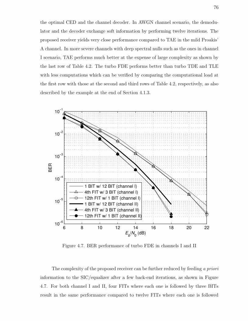
76
the optimal CED and the channel decoder. In AWGN channel scenario, the demodu-
lator and the decoder exchange soft information by performing twelve iterations. The
proposed receiver yields very close performance compared to TAE in the mild Proakis’
A channel. In more severe channels with deep spectral nulls such as the ones in channel
I scenario, TAE performs much better at the expense of large complexity as shown by
the last row of Table 4.2. The turbo FDE performs better than turbo TDE and TLE
with less computations which can be verified by comparing the computational load at
the first row with those at the second and third rows of Table 4.2, respectively, as also
described by the example at the end of Section 4.1.3.
6 8 10 12 14 16 18 20 2210−6
10−5
10−4
10−3
10−2
10−1
Eb/N
0 (dB)
BE
R
1 BIT w/ 12 BIT (channel I)4th FIT w/ 3 BIT (channel I)12th FIT w/ 1 BIT (channel I)1 BIT w/ 12 BIT (channel II)4th FIT w/ 3 BIT (channel II)12th FIT w/ 1 BIT (channel II)
Figure 4.7. BER performance of turbo FDE in channels I and II
The complexity of the proposed receiver can be further reduced by feeding a priori
information to the SIC/equalizer after a few back-end iterations, as shown in Figure
4.7. For both channel I and II, four FITs where each one is followed by three BITs
result in the same performance compared to twelve FITs where each one is followed

77
by one FIT, while the equalizer complexity is three times less for the former scenario.
Moreover, by exploiting the SISO capability of FDE, the performance gain of the
aforementioned scenarios compared to one FIT followed by twelve BITs is about 1 dB
after BER= 1 × 10⁻⁵ in both channels I and II.

78
5. ORTHOGONAL ST BLOCK CODING OF CPM ON
MULTIPATH FADING CHANNELS
This chapter presents an ST block coding scheme which preserves the spectral
efficiency of CPM perfectly and results in significant diversity gain for the frequency-
domain equalization of CPM signals transmitted over the multipath fading channels.
Contrary to the methods in [24]-[29] which operate in single-path flat fading channels
and depend on the ST coding of the information symbols before the CPM modula-
tion to maintain the phase continuity, the proposed method apply ST block coding
to CPM waveforms by assuming slowly-varying multipath fading channels which are
almost constant throughout two signal blocks. For this purpose, the scheme in [31] is
enhanced to maintain the bandwidth efficiency of CPM so that tail symbols are used
to prevent the phase discontinuities during the interblock transitions. Depending on
the orthogonality of the proposed scheme, the receiver complexity remains unchanged
whereas extra computations are required at the receiver for the methods in [24]-[29]
which can be viewed to be equivalent to ST trellis codes. Similar to the proposed
method, ST block coding in [30] is also applied directly to the CPM waveforms rather
than the information symbols. However, this method is not applicable in the presence
of frequency-selective multipath fading channels and it cannot preserve the constant
envelope and phase continuity during the interblock transitions which yields that the
spectral efficiency cannot be maintained perfectly.
The proposed scheme employs two transmit antennas. After the appropriate
low-pass filtering and sampling, the doubly-iterative receiver with FDE in Chapter 4 is
applied as in the case of single antenna transmissions depending on the orthogonal ST
combining. As shown in Figure 4.2, the receiver consists of a front-end soft-information
aided linear FDE filter, a central CPM demodulator, and a back-end channel decoder.
The demodulator computes soft information on both the CPM signals and the code bits.
Then, these two soft outputs are employed in a doubly-iterative information exchange
where the demodulator is coupled with both the FDE filter and the decoder. The

79
aforementioned receiver is preferred for its higher performance and lower complexity
compared to its counterpart in [23]. By using only one more transmit antenna to apply
the proposed ST block coding, it also attains superior performance and less complexity
than TAE coupling the optimal CED module in [10] with a back-end SISO decoder for
the turbo equalization of the coded CPM, as also verified by BER simulations.
The remainder of this chapter is organized as follows. Section 5.1 describes the
proposed ST block coding scheme and presents the orthogonal combining at the receiver
with the corresponding FDE filter coefficients. The simulation results are in Section
5.2.
5.1. Orthogonal ST Block Coding of CPM for Frequency-Domain
Equalization
The method in [31] proposes an Alamouti-like scheme for linear modulations
that combines the ST block coding with frequency-domain equalization. Defining
si,b := [s0,i,b s1,i,b . . . sN−1,i,b]T as the vector containing the symbols sn,i,b, which are
transmitted in the bth block from the ith antenna for b = 0, 2, 4, . . ., i ∈ {1, 2}, and
n = 0, 1, . . . , N − 1, the aforementioned scheme is applied as
s1,b+1(n) = −s∗2,b((−n)N),
s2,b+1(n) = s∗1,b((−n)N) (5.1)
where si,b(n) = sn,i,b is the nth entry of si,b, and (·)∗ and (·)N denote the complex
conjugate and modulo-N operations, respectively. Then, to eliminate the interblock
interference (IBI) and to obtain a simple representation for FDE, a length-G cyclic
prefix is appended to each block where G = max1≤i≤2dτNc,i−1,i/T e + 1 with d·e being
the ceiling operation. When the ST coding defined by (5.1) is applied directly to
the CPM signal in (2.1), the phase functions that correspond to the first and second

80
antennas before appending the cyclic prefix are computed as
ϕ(t + NT,x1,b+1) = −ϕ((−t)NT ,x2,b) + π,
ϕ(t + NT,x2,b+1) = −ϕ((−t)NT ,x1,b), (5.2)
respectively, which lead to
c(t + NT,x1,b+1) = −c∗((−t)NT ,x2,b),
c(t + NT,x2,b+1) = c∗((−t)NT ,x1,b), (5.3)
respectively, where 0 ≤ t ≤ NT and xi,b is the length-N symbol sequence for the CPM
modulation of the bth block at the ith transmit antenna.
As shown in (5.2), for each antenna, the signal phase at the (b + 1)th block is
negative compared to the one at the bth block. However, it is also reversed in time
which yields that the phase functions in the consecutive blocks belong to different
phase trees and, therefore, exact phase continuity cannot be guaranteed during the
interblock transitions. To circumvent this problem, the method in this dissertation is
devised properly so that the CPM signals at each transmit antenna are represented by
the same phase tree throughout all signal blocks. During interblock transitions and
cyclic prefix insertion, tail symbols are used to maintain the constant envelope and
phase continuity perfectly. After appropriate processing and sampling at the receiver,
an orthogonal discrete representation similar to (5.1) is obtained.
The proposed ST block coding scheme is described in Section 5.1.1 and the mod-
ifications for the FDE algorithm in Chapter 4 are presented in Section 5.1.2.
5.1.1. ST Block Coding for CPM
Denoting the length-N symbol sequences to be detected at the receiver through-
out two consecutive blocks as xj, j ∈ {1, 2}, the proposed method modifies these

81
sequences by inserting redundant symbols to maintain the phase continuity while ap-
pending the cyclic prefix and during the interblock transitions. The CPM signal trans-
onetail
symbol
xi,m(`)=xj(`−1)
` ≥ 2
` ≤ G−lt
lttail
symbols
onetail
symbol
xi,m(`) = xj(`− lt −2)
` ≥ G+2
` ≤ N−G+2lt +2
letail
symbols
xi,m(`) = xj(`− lt−le−2)
` ≥ N−G+ le +2lt +3
` ≤ N+ lt + le+2
lttail
symbols
lf
tail
symbols
G symbols for
cyclic guard insertion
G symbols for
cyclic guard insertion
forinterblocktransition
Figure 5.1. Modulating sequence for the ST block coding scheme with the cyclic
prefix
mitted in the mth block interval from the ith antenna is produced using the new symbol
sequence xi,m, m ∈ {b, b+1}, i ∈ {1, 2}, which is obtained from either x1 or x2 together
with the tail symbols according to the format illustrated in Figure 5.1. Because of the
time reversals, both the front and back parts of xi,m are arranged to keep the signal
phase continuous while appending a cyclic prefix. The last lf symbols in Figure 5.1
are for the maintenance of the phase continuity during the interblock transitions. The
details on how the new symbol sequences are generated are presented below.
The first element of x1,b is a tail symbol to stay at the zero state in (2.19) where the
initial state for the CPE trellis is also zero. After the first symbol, proceeding G− lt−1
elements of x1,b are set to be equal to the first G − lt − 1 symbols in x1 as Figure 5.1
implies. Then lt + 1 tail symbols are used to return to and stay at the zero state. For
G + 2 ≤ ` ≤ N − G + 2lt + 2, the sequence elements are set as x1,b(`) = x1(` − lt − 2)
and, after that, le ≥ lt tail symbols are used to return to and stay at the zero state.
Last G − lt symbols in x1 are exploited to obtain x1,b(`) = x1(` − lt − le − 2) where
N − G + le + 2lt + 3 ≤ ` ≤ N + lt + le + 2. Then lt tail symbols are used to return to
the zero state which is followed by lf ≥ lt tail symbols to go to and stay at the state
in (2.20) where the cumulative tilted phase is equal to π rather than zero. Similar
procedure is applied to obtain x2,b+1 and x2,b using x1 and x2, respectively, whereas
the only difference is employing lf tail symbols at the end to stay at the zero state. The
sequence x2,b is produced by using x2 where the initial state for the CPE trellis is set
as the state in (2.20) with first tail symbol keeping the trellis path at the same state.
Then lt +1 and le tail symbols shown in Figure 5.1 are used to return to and stay at the
state in (2.20) rather than the zero state. Furthermore, lt tail symbols return the trellis

82
path to the state in (2.20), whereas the last lf tail symbols are applied to go to and
stay at the zero state. The proposed ST block coding scheme requires the time-reversal
of the first N := N +2lt + le +2 symbols at the second antenna transmissions. That is
why the tail symbols to make the insertion of a cyclic guard interval possible without
phase discontinuities are applied at both the beginning and end of the symbol sequence
in Figure 5.1, which is not the case for single antenna transmissions as shown in Figure
4.1. Denoting the overall block length with the cyclic prefix as N ′ := N + lf + G, le
and lf are set properly so that h(M − 1)N and h(M − 1)N ′ is an even number which
yields that (πh(M − 1)N)2π = (πh(M − 1)N ′)2π = 0. Depending on this property and
after appending the cyclic guard intervals, the CPM phase functions for each antenna
and block which are obtained from the corresponding tilted-phase functions using the
relation in (2.15) are equal to
ϕ1,b(t) :=ϕ(t + (N − G)T, x1,b),
ϕ1,b+1(t + N ′T ) :=ϕ(t + (N − G)T, x1,b+1),
ϕ2,b(t) :=−ϕ(−t + GT, x2,b),
ϕ2,b+1(t + N ′T ) :=−ϕ(−t + GT, x2,b+1), (5.4)
on the interval 0 ≤ t ≤ GT ,
ϕ1,b(t) :=ϕ(t − GT, x1,b)
= −ϕ2,b+1(−t + (N ′ + N + 2G)T ),
ϕ1,b+1(t+N ′T ) :=ϕ(t − GT, x1,b+1)
= −ϕ2,b(−t + (N + 2G)T ) + π,
ϕ2,b(t) :=−ϕ(−t + (N + G)T, x2,b),
ϕ2,b+1(t+N ′T ) :=−ϕ(−t + (N + G)T, x2,b+1), (5.5)

83
on the interval GT ≤ t ≤ (N + G)T , and
ϕ1,b(t) :=ϕ(t − GT, x1,b),
ϕ1,b+1(t+N ′T ) :=ϕ(t − GT, x1,b+1),
ϕ2,b(t) :=−ϕ(−t+(N ′+N)T, x2,b),
ϕ2,b+1(t+N ′T ) :=−ϕ(−t+(N ′+N)T, x2,b+1), (5.6)
on the interval (N + G)T ≤ t ≤ N ′T . For all phase functions in (5.4)-(5.6), phase
continuity is maintained since it is assured by tail symbols in Figure 5.1 that the
CPE trellis path terminates at and continues from the same state at t = 0, t = GT ,
t = (N + G)T , and t = N ′T . Contrary to (5.2), because the time-reversal is applied
throughout all blocks at the second antenna, the corresponding phase functions belong
to the same phase tree which guarantees that the proposed method has no impact on
the spectral efficiency of the CPM scheme used. Furthermore, as shown in Appendix
C, the time-reversed phase functions can be produced by a finite-state machine as in
(2.2) so that it is not necessary to store and then reverse the real-time CPM signals .
Using the phase functions above, the corresponding ST-block coded CPM signals
are produced as
c1,b(t) := ejϕ1,b(t),
c1,b+1(t + N ′T ) := ejϕ1,b+1(t+N ′T ),
c2,b(t) := ejϕ2,b(t−Ts),
c2,b+1(t + N ′T ) := ejϕ2,b+1(t−Ts+N ′T ), (5.7)
respectively, on the interval 0 ≤ t ≤ N ′T . Here a time shift of Ts seconds is applied
to the signals transmitted from the second antenna, which is necessary to obtain an
appropriate discrete representation at the receiver. The tail symbol following the first
G symbols in Figure 5.1 compensates for the disrupting effects of the aforementioned
time shift on the phase continuity while adding the cyclic guard intervals to the time-
reversed signals at the second antenna.
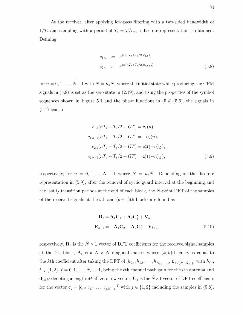
84
At the receiver, after applying low-pass filtering with a two-sided bandwidth of
1/Ts and sampling with a period of Ts = T/ns, a discrete representation is obtained.
Defining
c1,n := ejϕ(nTs+Ts/2,x1,b),
c2,n := ejϕ(nTs+Ts/2,x1,b+1) (5.8)
for n = 0, 1, . . . , N−1 with N = nsN , where the initial state while producing the CPM
signals in (5.8) is set as the zero state in (2.19), and using the properties of the symbol
sequences shown in Figure 5.1 and the phase functions in (5.4)-(5.6), the signals in
(5.7) lead to
c1,b(nTs + Ts/2 + GT ) = c1(n),
c1,b+1(nTs + Ts/2 + GT ) = −c2(n),
c2,b(nTs + Ts/2 + GT ) = c∗2((−n)N),
c2,b+1(nTs + Ts/2 + GT ) = c∗1((−n)N), (5.9)
respectively, for n = 0, 1, . . . , N − 1 where N = nsN . Depending on the discrete
representation in (5.9), after the removal of cyclic guard interval at the beginning and
the last lf transition periods at the end of each block, the N -point DFT of the samples
of the received signals at the bth and (b + 1)th blocks are found as
Rb = Λ1C1 + Λ2C∗2 + Vb,
Rb+1 = −Λ1C2 + Λ2C∗1 + Vb+1, (5.10)
respectively, Rb is the N × 1 vector of DFT coefficients for the received signal samples
at the bth block, Λi is a N × N diagonal matrix whose (k, k)th entry is equal to
the kth coefficient after taking the DFT of [h0,i, h1,i, . . . , hNc,i−1,i, 01×(N−Nc,i)] with h`,i,
i ∈ {1, 2}, ` = 0, 1, . . . , Nc,i−1, being the `th channel path gain for the ith antenna and
01×M denoting a length-M all-zero row vector, Cj is the N×1 vector of DFT coefficients
for the vector cj = [cj,0 cj,1 . . . cj,N−1]T with j ∈ {1, 2} including the samples in (5.8),
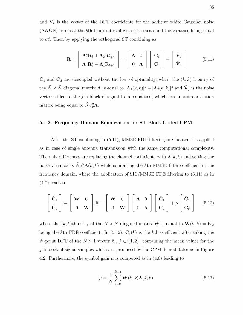
85
and Vb is the vector of the DFT coefficients for the additive white Gaussian noise
(AWGN) terms at the bth block interval with zero mean and the variance being equal
to σ2v . Then by applying the orthogonal ST combining as
R =
Λ∗
1Rb + Λ2R∗b+1
Λ2R∗b − Λ∗
1Rb+1
=
Λ 0
0 Λ
C1
C2
+
V1
V2
(5.11)
C1 and C2 are decoupled without the loss of optimality, where the (k, k)th entry of
the N × N diagonal matrix Λ is equal to |Λ1(k, k)|2 + |Λ2(k, k)|2 and Vj is the noise
vector added to the jth block of signal to be equalized, which has an autocorrelation
matrix being equal to Nσ2vΛ.
5.1.2. Frequency-Domain Equalization for ST Block-Coded CPM
After the ST combining in (5.11), MMSE FDE filtering in Chapter 4 is applied
as in case of single antenna transmission with the same computational complexity.
The only differences are replacing the channel coefficients with Λ(k, k) and setting the
noise variance as Nσ2vΛ(k, k) while computing the kth MMSE filter coefficient in the
frequency domain, where the application of SIC/MMSE FDE filtering to (5.11) as in
(4.7) leads to
C1
C2
=
W 0
0 W
R −
W 0
0 W
Λ 0
0 Λ
C1
C2
+ µ
C1
C2
(5.12)
where the (k, k)th entry of the N × N diagonal matrix W is equal to W(k, k) = Wk
being the kth FDE coefficient. In (5.12), Cj(k) is the kth coefficient after taking the
N -point DFT of the N × 1 vector cj, j ∈ {1, 2}, containing the mean values for the
jth block of signal samples which are produced by the CPM demodulator as in Figure
4.2. Furthermore, the symbol gain µ is computed as in (4.6) leading to
µ =1
N
N−1∑
k=0
W(k, k)Λ(k, k). (5.13)

86
Using the doubly-iterative structure presented in Section 4.1.1, the FDE filter
coefficients must be updated at each equalizer iteration since Ci changes at each iter-
ation. However this complexity is reduced as described in Section 4.1.1 and Appendix
B by computing two different sets of equalizer coefficients under either FAI or ZAI
scenarios which correspond to Cj = 0N×1 and Cj = Cj, respectively, and by starting
the initial FDE iterations with the ZAI coefficients and then switching to the FAI co-
efficients after a few iterations. Using the same procedure described in Appendix B by
replacing Hk with Λ(k, k) and updating the variance of the kth additive noise term in
the frequency domain as Nσ2vΛ(k, k), the FDE coefficients after the ST combining are
computed under the ZAI and FAI assumptions as
WZAI(k, k) =1
Λ(k, k) + σ2v
, (5.14)
WFAI(k, k) =1
Nσ2v + (1/N)
∑N−1m=0 Λ(m,m)
, (5.15)
respectively. The equalizer outputs c1 and c2 in time domain are obtained by applying
N -point IDFT operation to C1 and C2, respectively, which are exploited to compute
sample probabilities in (4.14) delivered to the demodulator for each signal block. The
switching condition from the ZAI to FAI coefficients are determined by comparing the
transfer characteristic curves of the FDE filter for each scenario, as in Figure 4.3 by
computing AD and AE as in (4.15) and (4.16), respectively, where the mean values
from the CPM demodulator are generated artificially as described in Section 4.2. The
convergence analysis for back-end iterations is also the same as in Section 4.2.
5.2. Simulation Results
In this section, the BER performance of the proposed orthogonal ST block cod-
ing scheme for CPM which is combined with the turbo FDE method in Chapter 5 is
presented for different number of front- and back-end iterations, and is also compared
to the case without ST combining, to the performance of TAE cascading the SISO op-
timal CED module in [10] with a back-end channel decoder, and to the performance for
the coded CPM in AWGN channel where the receiver consists of a SISO demodulator

87
followed by a SISO decoder. The 3RC CPM with L = 3 and h = 0.5 is considered as in
[2] with ns = 2, the two-sided bandwidth of the low-pass filter is 2/T , and the channel
resolution is Ts = T/2, as in [23]. The rate-1/2 convolutional code with generator
polynomial (64, 74)8 is used and random interleaving is applied. The aforementioned
methods with turbo equalizers are compared in an eleven-tap quasi-static channel en-
vironment, where the tap coefficients are zero-mean complex white Gaussian random
variables with exponentially decaying power profile such that the variance of the mth
path coefficient is e−m/2/( ∑10
l=0 e−l/2)
and the corresponding path delay is mTs for
m = 0, 1, . . . , 10.
2 4 6 8 10 12 14
10−6
10−5
10−4
10−3
10−2
10−1
100
101
Eb/ N
0 (dB)
BER
no ISI (12 iterations)TAE (12 iterations)turbo FDE (12 FIT w/ 1 BIT)turbo FDE w/ ST combining (12 FIT w/ 1 BIT)
1st Iteration
1st Iteration
12th Iteration
12th Iteration
1st FIT w/ 1 BIT
12th FIT w/ 1 BIT
Figure 5.2. BER performance for the turbo FDE with/without ST combining, TAE,
and no ISI scenario
In Figure 5.2, the BER performance of the turbo FDE with the ST combining is
compared to the those of the turbo FDE without the ST combining and the TAE by
using the aforementioned multipath fading channels. The turbo FDE exploits double
iterations where each FIT is followed by one BIT between the CPM demodulator and
the channel decoder whether the proposed ST coding scheme is applied or not. The

88
TAE conducts twelve iterations between the optimal CED and the channel decoder. In
AWGN channel scenario, the demodulator and the decoder exchange soft information
by performing twelve iterations. As shown in Figure 5.2, after applying the ST block
coding scheme, the error performance of the turbo FDE is improved significantly where
the performance gap is almost 5 dB at BER= 1 × 10⁻³ after the twelve FITs with
each being followed by one BIT. Furthermore, the performance of the turbo FDE with
ST coding is also much better than that of the TAE in the expense of deploying only
one more transmit antenna. On the other hand, the receiver complexity for TAE is
exponentially increasing by the length of the channel because of the trellis-based CED
module it employs. The complexity for the FDE filter is independent of the channel
memory.
4 6 8 10 12 1410−6
10−5
10−4
10−3
10−2
10−1
Eb/N
0 (dB)
BE
R
12th FIT w/ 1 BIT4th FIT w/ 3 BITs1 FIT w/12 BITs
Figure 5.3. BER performance for the turbo FDE with ST combining
The complexity of the proposed receiver can be further reduced by feeding a
priori information to the SIC/equalizer after a few BITs, as shown in Figure 5.3. For
the eleven-tap multipath fading channels, four FITs where each one is followed by

89
three BITs result in the same performance compared to twelve FITs where each one is
followed by one BIT, while the equalizer complexity is three times less for the former
scenario, as in Section 4.3. Moreover, by exploiting the SISO capability of FDE, the
performance gain of the aforementioned scenarios compared to one FIT followed by
twelve BITs is about 0.75 dB after BER= 1×10⁻³. In this way, the overall complexity
of the turbo FDE is reduced while its performance with ST coding is significantly
better than TAE.

90
6. ST PRE-EQUALIZATION OF CPM ON MULTIPATH
FADING CHANNELS
Optimal joint equalization and demodulation of CPM on frequency-selective mul-
tipath fading channels entails an intensive search over a single super trellis, which
combines the memory effects of both the modulator and the intersymbol interference
(ISI) channel [10]. Application of the reduced-state adaptive trellis search algorithms
as in [16, 17] for the joint detection of CPM results in lower complexity and does not
require channel state information (CSI). However, the computational load could still
be prohibitively large to obtain a good performance for channels with long impulse
responses. To circumvent the complexity limitations of the aforementioned methods,
the receivers proposed in Chapter 3 and 4, [18], [22], and [23] separate the equalization
and demodulation functions and employ a linear equalizer at the front-end before the
trellis-based CPM demodulation.
Application of channel precoding (or pre-equalization) at the transmitter reduces
the complexity further for receivers with limited resources [32]. TH-type precoders in
[33, 34] employ modulo-arithmetic operations to maintain the stability of the trans-
mitter, whereas direct application of the TH method to phase-modulated waveforms
results in large envelope fluctuations and destroys the spectral efficiency. As previously
mentioned, dimension partitioning is applied to MSK in [36]. However, this type of
pre-equalization is not applicable to other CPM schemes in general since they can-
not be represented by square signal constellations. Furthermore, frequency-domain
pre-equalizers in [37] and [38], and combined equalizers in [39] and [40] that consider
pre-equalization at the transmitter and post-equalization at the receiver to increase
the channel capacity rather than to reduce the receiver complexity cannot manage to
maintain the spectral efficiency of CPM since they result in variations in the signal
envelope and discontinuities in the signal phase. Although the precoders proposed for
CPM in [41]-[45] exhibit good spectral efficiency, these methods aim to equalize the
inherent ISI due to modulation memory and are not applicable for multipath channels.
91
This chapter presents a ST pre-equalization scheme for CPM which maintains
the spectral efficiency while mitigating the ISI effects of the multipath fading channels.
By applying a selection diversity technique, one of the antennas is chosen for the
transmission of the CPM signal while the rest of the antennas are used to transmit
the precoded signals to suppress the ISI. The signals for ISI cancellation are shaped
as the CPM signal added to a residual signal with small envelope variations such that
the narrow-band property of CPM is satisfied by attaining a PAPR close to one. The
proposed method considers a time-division duplex (TDD) system where the transmitter
and the receiver operate alternately in the same frequency band. Then, by assuming a
slowly-varying multipath fading process that is approximately constant throughout two
data packets, channel information that is obtained from the received packets is used
to pre-equalize the transmitted packets since the forward and reverse radio frequency
(RF) links are reciprocal according to the reciprocity theorem [69, 70]. The proposed
scheme depends on the approximation of CPM signals by using nSnOEE in [57], which
provides high accuracy and low complexity by employing a few basis functions as
described in Section 2.1.2. For pre-equalization, the ISI is computed and projected
onto the basis functions, where the projection coefficients are truncated using modulo-
arithmetic operations as in TH-type precoding to ensure stability. In the modulo
operations, a scaling parameter is employed to shorten the range of values for the
truncated coefficients, which is computed depending on the proposed transmit selection
diversity scheme. Then, the truncated projection coefficients are used to obtain the
spectrally-efficient signals for ISI cancellation. At the receiver, perfect synchronization
is assumed, and a bank of filters matched to the aforementioned basis functions is
employed. The only channel information that must be determined is the amplitude
of the fading path with the smallest propagation delay between the selected transmit
antenna and the receive antenna, which is estimated by using a training sequence. After
applying modulo operations, the projection coefficients for CPM signals are estimated
and fed to the CPM demodulator.
An upper bound on the error performance of the proposed system is computed
depending on the modulo operation errors at the receiver. The effect of the number
of transmit antennas on the spectral efficiency of the system is analyzed. In the sim-

92
ulations, the envelope variations and the power spectrum of the precoded signals are
depicted for different values of the system parameters. BER performance is presented
for different number of antennas and different channel and bandwidth scenarios. The
upper bound is shown to be consistent with the simulation results. Because transferring
the equalization functions reduces the complexity significantly, a turbo receiver is also
considered for coded CPM by performing iterations between the CPM demodulator
and the channel decoder, which are both implemented by the Log-BCJR algorithm as
described in Section 2.2.
The remainder of this chapter is organized as follows. Section 6.1 presents the
proposed channel precoding scheme and the design of the training sequence. Analyses
for the error performance and the number of transmit antennas required by the system
are described in Section 6.2. Section 6.3 presents the simulation results.
6.1. Space-Time Pre-Equalization of Continuous Phase Modulation
At the beginning of this section, the TH-type pre-equalization of CPM in the
presence of a single transmit antenna is described while the resulting precoded signal
is stated to encounter large envelope variations that disrupt the spectral efficiency.
Then, the space-time pre-equalizer is proposed so as to alleviate the envelope variations
of the precoded signals by using a scaling factor that is determined depending on a
transmit selection diversity scheme. The selected antenna transmits the CPM signal
while the rest of the antennas transmit the spectrally-efficient precoded signals that
are used to suppress the ISI at the receiver. At the end of the section, the design
of the training sequence to estimate the amplitude of the first fading path between
the selected transmit antenna and the receive antenna is presented. This amplitude
information is the only channel parameter that must be known for the detection of
CPM signals at the receiver.
The multipath channel in (2.23) fades slowly such that it is assumed to be time-

93
invariant throughout the duration of two data packets and is represented as
h(t) =Lc−1∑
`=0
h`δ(t − τ`) (6.1)
where Lc is the number of paths, h` and τ` are the fading coefficient and the propagation
delay for the `th path, respectively, and h` = ρ`ejθ` with ρ` and θ` denoting the
amplitude and the phase of the `th path, respectively. The proposed method requires
that the ISI on a symbol interval depends on the past symbols only, as in [35] and
[36]. Therefore, it is assumed that τ` − τ0 ≥ T for ` = 1, . . . , Lc − 1. For simplicity,
τ0 is assumed to be zero in the rest of the paper. Similar to [35] and [36], the channel
information is perfectly obtained from the received packet at the transmitter and is
used for pre-equalization of the downlink packet.
For the single antenna transmission, the CPE output signal y(t,xk1) in (2.14)
is pre-equalized to form z(t). The ISI signal obtained after the transmission of z(t)
through the multipath fading channels is expressed as
I(t) =Lc−1∑
`=1
h`z(t − τ`) (6.2)
assuming that the channel coefficients h` are properly scaled to compensate for the
shift in (2.14). A linear precoder with a transfer function equal to the inverse of the
channel transfer function yields z(t) = e−jθ0(y(t,xk
1) − I(t))/ρ0 and results in perfect
ISI cancellation without any processing at the receiver. However, such a precoder is
not stable unless all the zeros of the channel transfer function are inside the unit circle
[35, 36]. To circumvent the stability problems, a non-linear precoder can be used, as in
TH-type precoding. For this purpose, time-invariant complex coefficients are obtained
by the projection of I(t) in (6.2) onto the orthonormal basis functions in (2.27), which
leads to
Ik,i =
∫ kT
(k−1)T
I(t)φ∗i
(t − (k − 1)T
)dt, i = 1, . . . , Nb, (6.3)
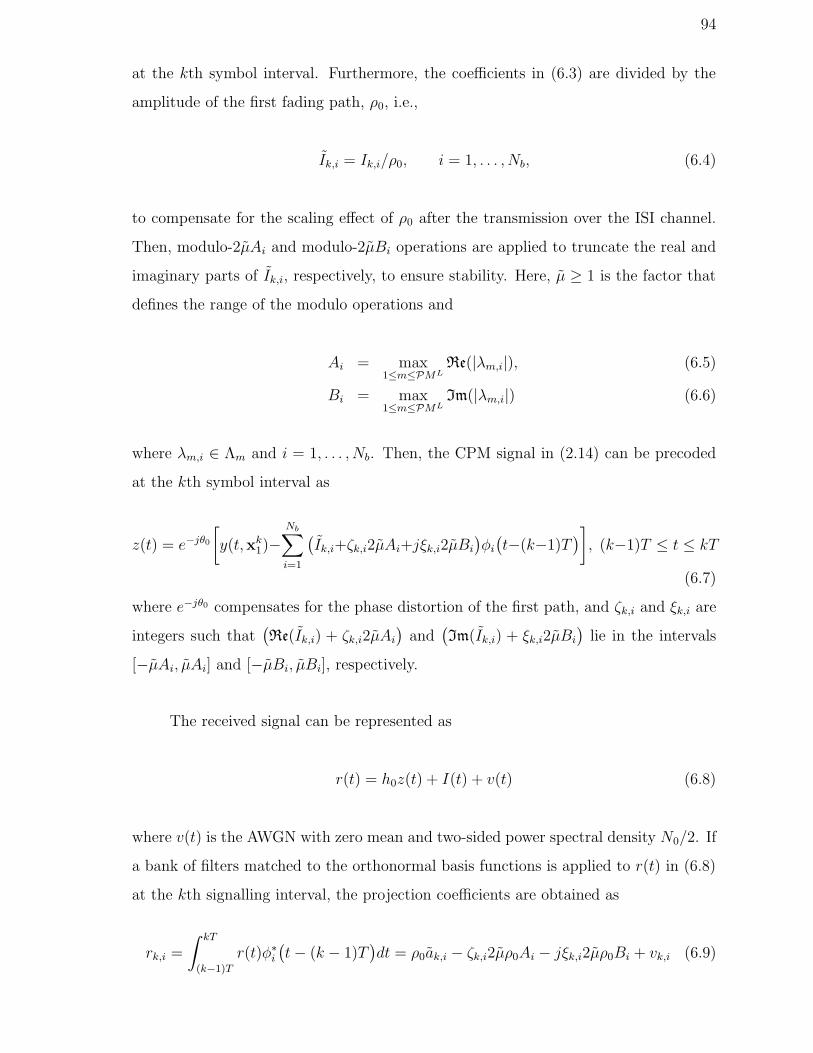
94
at the kth symbol interval. Furthermore, the coefficients in (6.3) are divided by the
amplitude of the first fading path, ρ0, i.e.,
Ik,i = Ik,i/ρ0, i = 1, . . . , Nb, (6.4)
to compensate for the scaling effect of ρ0 after the transmission over the ISI channel.
Then, modulo-2µAi and modulo-2µBi operations are applied to truncate the real and
imaginary parts of Ik,i, respectively, to ensure stability. Here, µ ≥ 1 is the factor that
defines the range of the modulo operations and
Ai = max1≤m≤PML
Re(|λm,i|), (6.5)
Bi = max1≤m≤PML
Im(|λm,i|) (6.6)
where λm,i ∈ Λm and i = 1, . . . , Nb. Then, the CPM signal in (2.14) can be precoded
at the kth symbol interval as
z(t) = e−jθ0
[
y(t,xk1)−
Nb∑
i=1
(Ik,i+ζk,i2µAi+jξk,i2µBi
)φi
(t−(k−1)T
)]
, (k−1)T ≤ t ≤ kT
(6.7)
where e−jθ0 compensates for the phase distortion of the first path, and ζk,i and ξk,i are
integers such that(Re(Ik,i) + ζk,i2µAi
)and
(Im(Ik,i) + ξk,i2µBi
)lie in the intervals
[−µAi, µAi] and [−µBi, µBi], respectively.
The received signal can be represented as
r(t) = h0z(t) + I(t) + v(t) (6.8)
where v(t) is the AWGN with zero mean and two-sided power spectral density N0/2. If
a bank of filters matched to the orthonormal basis functions is applied to r(t) in (6.8)
at the kth signalling interval, the projection coefficients are obtained as
rk,i =
∫ kT
(k−1)T
r(t)φ∗i
(t − (k − 1)T
)dt = ρ0ak,i − ζk,i2µρ0Ai − jξk,i2µρ0Bi + vk,i (6.9)

95
where the AWGN term vk,i =∫ kT
(k−1)Tv(t)φ∗
i
(t−(k−1)T
)dt has zero mean and variance
N0, and E[vk,iv∗k,l] = 0 if i 6= l. The real and imaginary parts of ρ0ak,i can be estimated
by applying modulo-2µρ0Ai and modulo-2µρ0Bi operations to those of rk,i, respectively.
Because Ai and Bi denote the maximum absolute values that are obtained from the
real and imaginary parts of the CPM projection coefficients for the ith basis function,
respectively, no signal information is lost at the receiver when the additive noise is
zero. However, the basis functions with the truncated coefficients in (6.7) result in
huge envelope fluctuations and, thus, z(t) cannot attain the narrow-band property of
a CPM signal.
The ST pre-equalizer is proposed to meet the bandwidth requirements of CPM
with small envelope variations, which uses a transmit selection diversity scheme to
replace the signal for ISI cancellation in (6.7) by the CPM waveform in (2.14) and a
residual signal. The signal for ISI cancellation is obtained as follows.
Considering NT transmit antennas, the ISI in (6.2) is modified as
I(t) =
NT∑
p=1
Lc−1∑
`=1
h`,pzp(t − τ`,p) (6.10)
where h`,p is the `th path coefficient that corresponds to the pth antenna with h`,p =
ρ`,pejθ`,p , τ`,p is the `th path delay that corresponds to the pth antenna, and zp(t) is the
precoded signal transmitted from the pth antenna. The antenna selection is performed
by choosing the first path amplitude that minimizes the distance below as
s := arg min1≤p≤Nt
∣∣∣∣ρ0,p −
ρT
ν + 1
∣∣∣∣
(6.11)
where s is the index of the chosen antenna, ρT =∑NT
p=1 ρ0,p is the sum of the first path
amplitudes for all transmit antennas, and ν > 1 is a parameter to control the envelope
variations. Using I(t) in (6.10), {Ik,i} are found as in (6.3), and (6.4) is modified as
Ik,i =
√NT Ik,i
ρT − ρ0,s
, i = 1, . . . , Nb. (6.12)

96
Then, defining
Dk,i := ak,i + Ik,i, (6.13)
γ := (ρ0,s)/(ρT − ρ0,s), (6.14)
modulo-2µAiγ and modulo-2µBiγ operations are applied to the real and imaginary
parts of Dk,i, respectively, which leads to
κk,i = ak,i + Ik,i + ζk,i2µAiγ + jξk,i2µBiγ (6.15)
where ζk,i and ξk,i are integers such that Re(κk,i) and Im(κk,i) lie in the intervals
[−µAiγ, µAiγ] and [−µBiγ, µBiγ], respectively. The γ ratio in (6.14) is the scaling
CPE PrecoderSwitching
Device
AntennaSelectionModule
γ s
ChannelInformation
{h`,p} {ρ0,p} {ejθ0,p}
Tx1
ej2π(fc−
h(M−1)2T
)t
e−jθ0,1√
NT
[
y(t, xk1 ) + κ(t)
]
Txs
ej2π(fc−
h(M−1)2T
)t
e−jθ0,s√
NTy(t, xk
1 ) TxNT
ej2π(fc−
h(M−1)2T
)t
e−jθ0,NT√
NT
[
y(t, xk1 ) + κ(t)
]
xk1 y(t, xk
1 ) κ(t)
Space-Time Pre-Equalizer
Figure 6.1. Space-time CPM pre-equalizer
factor that alleviates the envelope variations. Defining the residual signal as
κ(t) := −Nb∑
i=1
κk,iφi
(t − (k − 1)T
), (k − 1)T ≤ t ≤ kT, (6.16)

97
the signal for ISI cancellation is obtained as y(t,xk1) + κ(t) whose projection onto the
orthonormal bases yields the complex coefficients, (−Ik,i − ζk,i2µAiγ − jξk,i2µBiγ),
for i = 1, . . . , Nb. For further spectral efficiency, the residual signal, κ(t), is low-pass
filtered with negligible energy loss to form κ(t).
As shown in Figure 6.1, the sth antenna chosen using (6.11) transmits the CPM
signal as
zs(t) =e−jθ0,s
√NT
y(t,xk1), (k − 1)T ≤ t ≤ kT, (6.17)
and, for 1 ≤ p ≤ NT and p 6= s, the corresponding antennas transmit the signals for
ISI cancellation as
zp(t) =e−jθ0,p
√NT
[
y(t,xk1) + κ(t)
]
, (k − 1)T ≤ t ≤ kT (6.18)
where 1/√
NT in (6.17) and (6.18) is for energy scaling. After applying matched filtering
to the received signal as in (6.9), we obtain
rk,i =ρ0,s√NT
[
ak,i − ζk,i2µAi − jξk,i2µBi
]
+ vk,i. (6.19)
Then, assuming that ρ0,s is available at the receiver, the real and imaginary parts of
ρ0,sak,i/√
NT are found by applying modulo-2µρ0,sAi/√
NT and modulo-2µρ0,sBi/√
NT
operations to those of rk,i, respectively. When the minimum distance in (6.11) is close
to zero, γ is approximately equal to 1/ν. Then the residual component in (6.18)
diminishes by increasing ν, which also improves the spectral efficiency of the signal,
as also shown in Section 6.3. However, as observed in (6.11), it is more probable to
choose a deep fading first path coefficient as ν increases. Therefore, there is a tradeoff
between the power efficiency of the system and the PAPR of the precoded signal in
(6.18).
The transmitter sends the value of ρ0,s to the receiver for the estimation of {ak,i}in (6.19). For this purpose, ρ0,s is quantized by considering V = 2J decision levels,
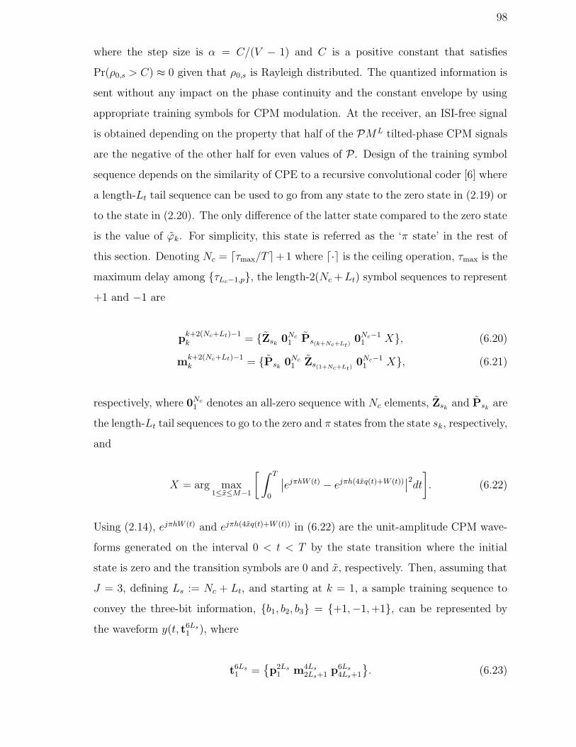
98
where the step size is α = C/(V − 1) and C is a positive constant that satisfies
Pr(ρ0,s > C) ≈ 0 given that ρ0,s is Rayleigh distributed. The quantized information is
sent without any impact on the phase continuity and the constant envelope by using
appropriate training symbols for CPM modulation. At the receiver, an ISI-free signal
is obtained depending on the property that half of the PML tilted-phase CPM signals
are the negative of the other half for even values of P . Design of the training symbol
sequence depends on the similarity of CPE to a recursive convolutional coder [6] where
a length-Lt tail sequence can be used to go from any state to the zero state in (2.19) or
to the state in (2.20). The only difference of the latter state compared to the zero state
is the value of ϕk. For simplicity, this state is referred as the ‘π state’ in the rest of
this section. Denoting Nc = dτmax/T e+1 where d·e is the ceiling operation, τmax is the
maximum delay among {τLc−1,p}, the length-2(Nc + Lt) symbol sequences to represent
+1 and −1 are
pk+2(Nc+Lt)−1k = {Zsk
0Nc1 Ps(k+Nc+Lt)
0Nc−11 X}, (6.20)
mk+2(Nc+Lt)−1k = {Psk
0Nc1 Zs(1+Nc+Lt)
0Nc−11 X}, (6.21)
respectively, where 0Nc1 denotes an all-zero sequence with Nc elements, Zsk
and Pskare
the length-Lt tail sequences to go to the zero and π states from the state sk, respectively,
and
X = arg max1≤x≤M−1
[ ∫ T
0
∣∣ejπhW (t) − ejπh(4xq(t)+W (t))
∣∣2dt
]
. (6.22)
Using (2.14), ejπhW (t) and ejπh(4xq(t)+W (t)) in (6.22) are the unit-amplitude CPM wave-
forms generated on the interval 0 < t < T by the state transition where the initial
state is zero and the transition symbols are 0 and x, respectively. Then, assuming that
J = 3, defining Ls := Nc + Lt, and starting at k = 1, a sample training sequence to
convey the three-bit information, {b1, b2, b3} = {+1,−1, +1}, can be represented by
the waveform y(t, t6Ls1 ), where
t6Ls1 =
{p2Ls
1 m4Ls2Ls+1 p6Ls
4Ls+1
}. (6.23)

99
All the antennas transmit the same training sequence such that
zp(t) =e−jθ0,p
√NT
y(t, t6Ls1 ), 0 ≤ t ≤ 6LsT, p = 1, . . . , NT . (6.24)
At the receiver, the ISI-free signal is obtained as
r(t + (2i − 1)LsT − T
)+ r
(t + 2iLsT − T
)=
ρT√NT
(
ejπhW (t)+jπδ(bi+1)
+ ejπh(4Xq(t)+W (t))+jπδ(bi−1)
)
+ v(t + (2i − 1)LsT − T
)+ v
(t + 2iLsT − T
)(6.25)
where 0 ≤ t ≤ T , i = 1, 2, . . . , J , δ(·) is the Kronecker delta function, ejπhW (t)+jπ
and ejπh(4Xq(t)+W (t))+jπ are the tilted-phase CPM waveforms generated by the state
transitions where π state is the initial state and the transition symbols are 0 and X,
respectively, and bi ∈ {−1, +1}. Defining f(t) := ejπhW (t) − ejπh(4Xq(t)+W (t)), the bit
values and h0,s are computed as
bi = sgn
{ ∫ T
0
[
r(t + (2i − 1)LsT − T
)+ r
(t + 2iLsT − T
)]
f ∗(t)dt
}
, (6.26)
and
h0,s = αJ∑
i=1
bi2i−1, (6.27)
respectively, where bi = (bi + 1)/2. The duration of the training sequence to transmit
a J-bit label is J2Ls symbol periods.
6.2. Analyses for the Error Performance and the Number of Antennas
6.2.1. Upper Bound on the Error Performance
When the modulo operations are applied to rk,i in (6.19), errors are encountered
especially due to deep fading on the first channel path and/or large noise power, caus-

100
ing a non-Gaussian observation noise in projection coefficient estimates and, therefore,
deteriorating the system performance significantly. However, as the SNR increases and
fewer coefficient estimates are affected by additive non-Gaussian noise at each symbol
interval, more packets can be recovered without bit errors after CPM demodulation.
Thus, modulo operation errors dominate the system performance and the average prob-
ability of having modulo operation errors at a symbol interval throughout a packet can
be considered as an upper bound on the BER performance of the demodulator. Given
the transmitted CPM burst and ρ0,s, and considering the complex AWGN terms in
(6.19), whose real and imaginary parts are mutually independent with zero mean and
variance N0/2, the average conditional probability of having modulo operation errors
at a symbol interval is defined as
pme|ρ0,s,a :=1
N
N∑
k=1
pme|ρ0,s,ak(6.28)
where
pme|ρ0,s,ak= 1 − 1
πNT N0
N∑
k=1
Nb∏
i=1
∫ ρ0,sµAi
−ρ0,sµAi
e−
∣∣u−ρ0,sRe(ak,i)
∣∣2
NT N0 du
∫ ρ0,sµBi
−ρ0,sµBi
e−
∣∣v−ρ0,sIm(ak,i)
∣∣2
NT N0 dv
(6.29)
and u and v are the random variables to represent the real and imaginary parts of
ρ0,sak,i +√
NT vk,i, respectively. Then, the average probability of having a modulo
operation error is
pme =
∫ ∞
−∞
(∑
a
p(a)pme|ρ0,s,a
)
f(ρ0,s)dρ0,s (6.30)
where p(a) is the probability of having the projection coefficients a of the corresponding
CPM burst and f(ρ0,s) denotes the probability density function (pdf) of ρ0,s. Consider-
ing independent and identically distributed (i.i.d.) sequences of uniformly distributed
M -ary symbols, {xk}N1 , and starting CPM modulation at a certain state such as the

101
zero state, p(a) = 1/MN for all possible packets, and
∑
a
p(a)pme|ρ0,s,a =1
MN
∑
a
pme|ρ0,s,a. (6.31)
Furthermore, because the NMN waveforms generated by the aforementioned symbol
sequences are distributed almost uniformly over PML possible tilted phase CPM wave-
forms,
1
MN
∑
a
pme|ρ0,s,a ≈ 1
PML
PML∑
m=1
pme|ρ0,s,λm (6.32)
where
pme|ρ0,s,λm = 1 − 1
πNT N0
Nb∏
i=1
∫ ρ0,sµAi
−ρ0,sµAi
e−
∣∣u−ρ0,sRe(λm,i)
∣∣2
NT N0 du
∫ ρ0,sµBi
−ρ0,sµBi
e−
∣∣v−ρ0,sIm(λm,i)
∣∣2
NT N0 dv.
(6.33)
Then, from (6.30)-(6.32),
pme ≈1
PML
∫ ∞
−∞
( PML∑
m=1
pme|ρ0,s,λm
)
f(ρ0,s)dρ0,s. (6.34)
When the minimum distance in (6.11) is zero, the first fading path amplitude for the
selected antenna is found as
ρ0,s =ρT
ν + 1=
∑NT
p=1 ρ0,p
ν + 1(6.35)
where {ρ0,p} are i.i.d. Rayleigh random variables with variance (2 − π/2)σ2R. In [71],
an accurate closed-form pdf approximation for the sum of NT i.i.d. Rayleigh random
variables with variance (2 − π/2) is given as
fNT(ε) =
ε2NT−1e−ε2/(2b)
2NT−1bNt(NT − 1)!−(ε − a2)
2NT−2ea1(ε−a2)2/(2b)
2NT−1b(b/a1)NT (NT − 1)!×a0[b(2NT ε−a2)−a1ε(ε−a2)
2]
(6.36)

102
with
ε = ρ/√
NT (6.37)
where ρ is the sum of the random variables. The values of the coefficients b, a0, a1,
and a2 change by the number of random variables in the sum, and they are computed
in [71] for a wide range of NT values. Using the pdf in (6.36), pme can be numerically
computed as
pme ≈1
PML
∫ ∞
−∞
( PML∑
m=1
pme|ρ0,s,λm
)
fNT(ε)dε (6.38)
where it can be found that ρ0,s = σR
√NT ε/(ν + 1) by using the expressions in (6.35)
and (6.37).
6.2.2. Analysis for the Number of Antennas
The precoding scheme has to maintain small envelope variations for the spectral
efficiency as described in Section 6.1. For limiting the envelope variations successfully,
the minimum distance in (6.11) needs to be as small as possible so that the γ values in
(6.14) are not much larger than 1/ν. For a given value of ν, the mean of the normalized
minimum distance, D := |ρ0,s−ρT /(ν+1)|ρT /ν+1
, can be used as an information measure to be
evaluated for different NT values, where ρT =∑NT
p=1 ρ0,p as defined in Section 6.1. In
this way, the number of transmit antennas yielding the minimum mean value and,
thus, the most accurate γ ratios can be determined. Using (6.11), the mean of D is
computed as
E{D} := D =
∫ ∞
ρ0,NT=0
. . .
∫ ∞
ρ0,1=0
min1≤p≤Nt
∣∣ρ0,p − ρT /(ν + 1)
∣∣
ρT /(ν + 1)
f(ρ0,1|σ) . . . f(ρ0,NT|σ)dρ0,1 . . . dρ0,NT
(6.39)
where first fading path amplitudes with powers σ2 are assumed to be i.i.d. Rayleigh
random variables and f(ξ|σ) = (ξ/σ2)e−ξ2/2σ2. Then, using (6.39), D can be numer-

103
ically computed for different NT values and the number of antennas that results in
the minimum D value can be determined. However, the computation of D becomes
impractical as NT increases depending on the complexity of the integration operations
in (6.39). By simulating large enough number of samples and assuming a stationary
ergodic process, an accurate average can be used instead of (6.39). Then, considering
samples from the aforementioned Rayleigh distribution and denoting ρ0,p,i and ρT,i as
the ith sample for the pth first path amplitude and the sum of ith samples for NT first
path amplitudes, respectively, it can be concluded that
limm→∞
1
m
m∑
i=0
min1≤p≤Nt
∣∣ρ0,p,i − ρT,i/(ν + 1)
∣∣
ρT,i/(ν + 1)= D. (6.40)
For small values of NT , results obtained from (6.39) and (6.40) are also shown to be
consistent in Section 6.3.
6.3. Simulations
The modulation scheme used in the simulations is 4-ary 3RC CPM with h = 1/2
[2]. Three pulses are used for nSnOEE where the optimized set of frequencies is found
as {0.25/T, 0.95/T, 1/T} in [57]. The precoding parameter µ is set as 1.5. Prior to the
CPE block, the data bits are encoded according to a rate-1/2 convolutional code with
generator polynomial (7, 5)8. Then, the code bits are interleaved randomly. The dura-
tion of the packets is N = 256 symbol periods. The first path amplitude is estimated by
appending a training sequence to each packet, where J = 12. In the simulations, con-
tinuous time-varying channel coefficients are such that h`,p(t) = hr`,p(t)+ jhi
`,p(t) where
hr`,p(t) and hi
`,p(t) are zero-mean Gaussian random variables, E[hr`,p(t)h
i`,p(t + τ)] = 0,
E[hr`,p(t)h
r`,p(t + τ)] = E[hi
`,p(t)hi`,p(t + τ)] = σ2
`,pJ0(2πfmτ)/2, with J0(.) being the
zeroth order Bessel function of the first kind, fm being the maximum Doppler shift,
and σ2`,p being the power corresponding to `th path of the pth antenna. Furthermore
E[h`,p(t)h∗`′,p′(t+τ)] = 0 if ` 6= `′ and/or p 6= p′. The performance of the pre-equalizer is
compared to that of the FDE in [22], which considers a single antenna at the transmit-
ter and uses the aforementioned orthogonal bases for matched filtering at the receiver.
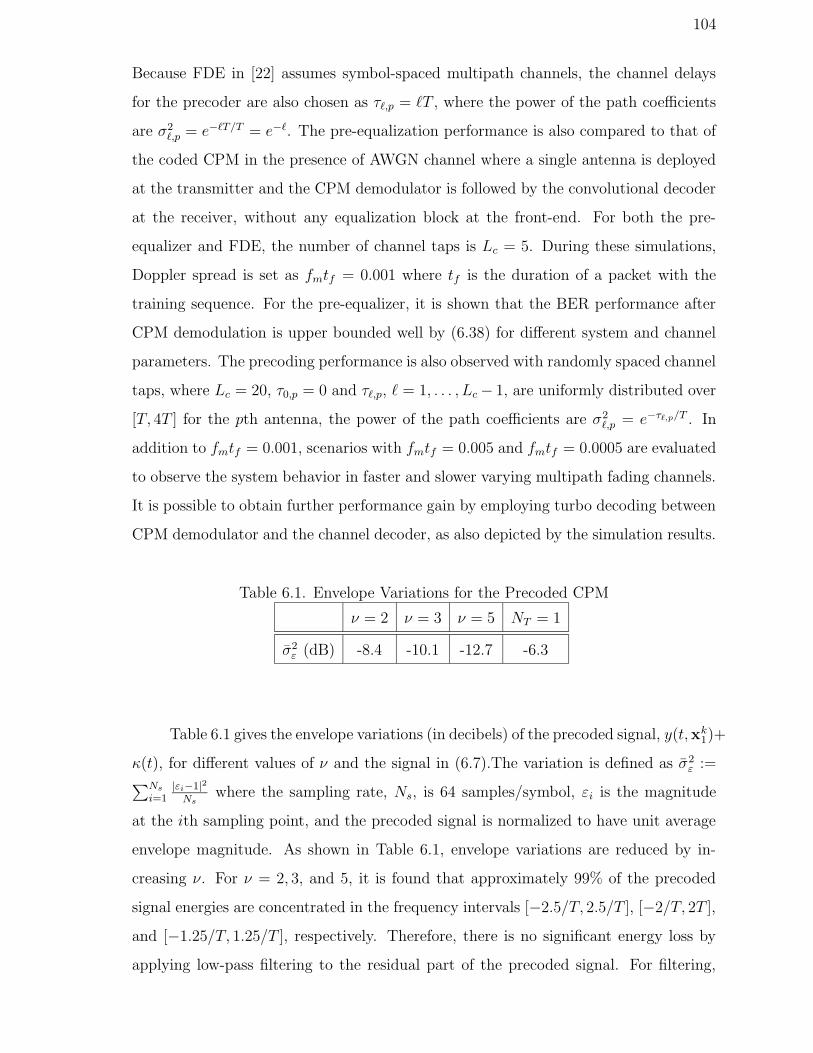
104
Because FDE in [22] assumes symbol-spaced multipath channels, the channel delays
for the precoder are also chosen as τ`,p = `T , where the power of the path coefficients
are σ2`,p = e−`T/T = e−`. The pre-equalization performance is also compared to that of
the coded CPM in the presence of AWGN channel where a single antenna is deployed
at the transmitter and the CPM demodulator is followed by the convolutional decoder
at the receiver, without any equalization block at the front-end. For both the pre-
equalizer and FDE, the number of channel taps is Lc = 5. During these simulations,
Doppler spread is set as fmtf = 0.001 where tf is the duration of a packet with the
training sequence. For the pre-equalizer, it is shown that the BER performance after
CPM demodulation is upper bounded well by (6.38) for different system and channel
parameters. The precoding performance is also observed with randomly spaced channel
taps, where Lc = 20, τ0,p = 0 and τ`,p, ` = 1, . . . , Lc − 1, are uniformly distributed over
[T, 4T ] for the pth antenna, the power of the path coefficients are σ2`,p = e−τ`,p/T . In
addition to fmtf = 0.001, scenarios with fmtf = 0.005 and fmtf = 0.0005 are evaluated
to observe the system behavior in faster and slower varying multipath fading channels.
It is possible to obtain further performance gain by employing turbo decoding between
CPM demodulator and the channel decoder, as also depicted by the simulation results.
Table 6.1. Envelope Variations for the Precoded CPM
ν = 2 ν = 3 ν = 5 NT = 1
σ2ε (dB) -8.4 -10.1 -12.7 -6.3
Table 6.1 gives the envelope variations (in decibels) of the precoded signal, y(t,xk1)+
κ(t), for different values of ν and the signal in (6.7).The variation is defined as σ2ε :=
∑Ns
i=1|εi−1|2
Nswhere the sampling rate, Ns, is 64 samples/symbol, εi is the magnitude
at the ith sampling point, and the precoded signal is normalized to have unit average
envelope magnitude. As shown in Table 6.1, envelope variations are reduced by in-
creasing ν. For ν = 2, 3, and 5, it is found that approximately 99% of the precoded
signal energies are concentrated in the frequency intervals [−2.5/T, 2.5/T ], [−2/T, 2T ],
and [−1.25/T, 1.25/T ], respectively. Therefore, there is no significant energy loss by
applying low-pass filtering to the residual part of the precoded signal. For filtering,

105
a square-root raised cosine pulse is employed where the roll-off factor is 0.25 and the
−4 −3 −2 −1 0 1 2 3 4−70
−60
−50
−40
−30
−20
−10
0
10
f T
Pow
er sp
ectru
m m
agni
tude
(dB
)
CPMprecoded CPM, ν = 5precoded CPM, ν = 3precoded CPM, ν = 2precoded CPM, N
T =1
Figure 6.2. Power spectra for the original and the precoded CPM signals
main lobe width is set appropriately according to the bandwidth requirements of each
case. The envelope variations are huge for the single antenna scenario. In Figure 6.2,
power spectra of the precoded signals in (6.18) and (6.7) are compared to the spectrum
of the original CPM signal by averaging the squared magnitude of the discrete Fourier
transform of different packets [2]. Considering the kth symbol interval and the ith
orthonormal basis function, the residual component in (6.16) corresponds to a square
waveform with complex gain, −κk,i, that is multiplied by the complex exponentials
in (2.9). The Fourier transform of this waveform is equivalent to the superposition
of sinc pulses that are shifted in the frequency domain by {fk} in (2.9), respectively.
Therefore, the power spectra for the precoded signals are asymmetric. The spectrum
for ν = 5 is almost the same as the spectrum of the original CPM signal. Decreasing
ν results in bandwidth expansion but it becomes less likely to choose a deep fading
first path coefficient as (6.11) yields. Therefore, there is a trade-off between the per-
formance and the bandwidth requirements. Furthermore, it is also possible to avoid
deep fading by increasing the number of transmit antennas while keeping ν constant

106
and maintaining the spectral efficiency. When the transmit selection diversity is not
used (NT = 1), bandwidth efficiency deteriorates.
2 4 6 8 10 12 14 16 18 200
0.2
0.4
0.6
0.8
1
1.2
NT
D
simulation results for ν =3numerical results for ν =3simulation results for ν =5numerical results for ν =5
Figure 6.3. Distance D versus Nt for ν = 3 and 5
It is also possible to avoid deep fading by deploying more transmit antennas
(which results in larger ρT ). However, the distance in (6.11) needs to be small enough
to maintain the spectral efficiency while increasing the number of antennas, as described
in Section 6.2.2. In Figure 6.3, change of D while increasing NT is depicted with ν
being equal to 3 and 5. Depending on the complexity issues, (6.40) is employed by
simulating one million samples for each antenna. Simulation results are consistent with
the numerical results found by (6.39) for up to six transmit antennas. As shown in
Figure 6.3, small D values must be considered to maintain the spectral efficiency while
determining the number of antennas.

107
5 10 15 20 25 3010−6
10−5
10−4
10−3
10−2
10−1
100
Eb/N
0 (dB)
BE
R
FDE (NT = 1)
NT = 4, ν = 5
NT = 6, ν = 5
NT = 8, ν = 5
NT = 4, ν = 3
NT = 6, ν = 3
NT = 8, ν = 3
no ISI (NT = 1)
Figure 6.4. BER performance for the no ISI scenario, FDE, and the pre-equalizers
In Figure 6.4, BER performance of the pre-equalizer is illustrated for different
values of NT and ν and is also compared to that of no ISI case and FDE. Both the
pre-equalizer with ν = 3 and NT = 8 and the FDE go below BER = 1 × 10⁻⁵ at
the same Eb/N0 value. However, signal bandwidth is almost extended twice, whereas
eight times more transmit antennas are deployed for pre-equalization. When ν = 5,
the performance gap between the pre-equalizer and FDE is about 6.5 dB and 3 dB at
BER = 1×10⁻⁵ for NT = 6 and NT = 8, respectively, while the gap is around 15 dB at
BER = 1 × 10⁻³ for NT = 4. The spectral efficiency is almost as same as the original
CPM signal as shown in Figure 6.2.

108
15 17 19 21 23 25 27 2910−6
10−5
10−4
10−3
10−2
10−1
100
Eb/N
0(dB)
BER
NT = 6, ν = 5
NT = 6, ν = 3
NT = 6, ν = 2
NT = 6, ν = 5 (p
me)
NT = 6, ν = 3 (p
me)
NT = 6, ν = 2 (p
me)
Figure 6.5. BER performance of the CPM demodulator and the upper bound, pme,
for NT = 6
15 17 19 21 23 25 27 2910−6
10−5
10−4
10−3
10−2
10−1
100
Eb/N
0(dB)
BER
NT = 4, ν = 5
NT = 6, ν = 5
NT = 8, ν = 5
NT = 4, ν = 5 (p
me)
NT = 6, ν = 5 (p
me)
NT = 8, ν = 5 (p
me)
Figure 6.6. BER performance of the CPM demodulator and the upper bound, pme,
for ν = 5
Performance-bandwidth and performance-spatial diversity trade-offs can also be

109
observed analytically by exploiting pme in (6.38). By setting the number of transmit
antennas as NT = 6, pme and BER performance after CPM demodulation are compared
for different bandwidth scenarios in Figure 6.5, where pme is consistent with the system
behavior and acts as an upper bound on the BER performance, as described in Section
6.2.1. Moreover, in Figure 6.6, pme and BER performance after CPM demodulation
are compared for different number of transmit antennas, where ν = 5. During the
simulations to obtain the BER performance for the CPM demodulator, ρ0,s is assumed
to be estimated perfectly and no low-pass filtering is applied to the residual signal to
satisfy the same assumptions while deriving (6.38). Both simulation scenarios justify
that the system performance depends on the modulo operation errors and pme can
be used to understand the system behavior for different pre-equalizer and channel
parameters. For NT = 4, pme is not exactly an upper bound on the BER curves. This
15 17 19 21 23 25 27 2910−6
10−5
10−4
10−3
10−2
10−1
100
Eb/N
0 (dB)
BE
R
fm
tf = 0.0005
fm
tf = 0.001
fm
tf = 0.005
Figure 6.7. BER for different maximum Doppler spread (fm) values, where NT = 6,
ν = 5, and Lc = 20
is because the derivation of pme considers that the minimum distance in (6.11) is zero.

110
However, as shown in Figure 6.3, D value is greater for NT = 4 than those for NT = 6
and NT = 8, respectively. Thus, because of larger deviations, it is more probable to
choose a deep fading first path and to encounter modulo operation errors (which result
in bit errors) compared to the theoretical results.
In Figure 6.7, the BER performance is also illustrated for different values of the
maximum Doppler spread, fm, where the aforementioned 20-tap multipath channels
are considered with NT = 6 and ν = 5. The performance at fmtf = 0.001 is almost
the same compared to the case where fmtf = 0.0005. An error floor is observed at
fmtf = 0.005. For coded CPM, further gain is observed by performing iterations
between the CPM demodulator and the channel decoder, which are both implemented
15 17 19 21 23 25 27 2910−5
10−4
10−3
10−2
10−1
100
Eb/N
0(dB)
FER
1st iteration2nd iteration3rd iteration
Figure 6.8. Turbo performance for fmtf = 0.001, NT = 6, ν = 5, and Lc = 20
by the BCJR algorithm [9]. In Figure 6.8, the frame error rate (FER) is shown for
20-tap multipath channels with fmtf = 0.001, NT = 6 and ν = 5, rather than the
BER performance. FER is preferred for better presentation purposes since the modulo

111
operation errors result in non-Gaussian noise at lower SNRs, which makes the BER
values increase after each iteration due to the incorrect modelling of the additive noise.
112
7. CONCLUSIONS
In this dissertaion, advanced transceiver designs are introduced for CPM on mul-
tipath fading channels by applying novel iterative and space-time methods. To reduce
the detection complexity while attaining near-optimal performance, turbo receivers us-
ing soft-information-aided linear TDE and FDE filters are proposed for bit-interleaved
coded CPM in Chapter 3 and 4, respectively. Then a ST block coding scheme is pro-
posed in Chapter 5 to improve the performance of the turbo FDE. In Chapter 6, a ST
pre-equalizer is proposed to mitigate the ISI effects of the multipath channel at the
transmitter to remove the equalization functions at the receiver.
The low-complexity turbo receiver in Chapter 3 consists of a SIC/MMSE TDE
at its front-end, and SISO demodulator and channel decoder blocks at its back-end.
Doubly-iterative processing overcomes the performance degradation resulting from the
suboptimality of the receiver. Performing a few BITs after each FIT, a priori infor-
mation for the equalizer is improved, and faster convergence to low bit error rates is
attained with less complexity. This behavior is also observed by EXIT chart analysis.
Contrary to the CED methods, the proposed receiver does not result in very large su-
per trellises with exponentially increasing number of states, which happens with longer
channel length or higher modulation memory.
In Chapter 4, the doubly-iterative receiver with a SISO frequency-domain MMSE
equalizer at the front-end is proposed for CPM with higher performance and less com-
plexity than its counterparts also employing linear equalizers, such as the doubly-
iterative receiver with TDE in Chapter 4 and TLE in [23] using a BFDE filter. For
the application of the FDE, a cyclic guard interval is appended to the transmitted
block by maintaining the phase continuity of CPM with each block and between the
consecutive blocks. The convergence behavior of the proposed receiver is determined
by EXIT chart analysis as in Chapter 3. Effectiveness of the new receiver is presented
with comparisons in terms of the overall computational complexity and the BER sim-
ulations.
113
By proposing an orthogonal ST block coding scheme for CPM in Chapter 5
which is combined with FDE at the receiver, significant diversity gain is obtained. The
proposed scheme is applied by maintaining the phase continuity of CPM where the
orthogonality allows the application of FDE as in case of single antenna transmissions.
By deploying only two transmit antennas, the proposed scheme combined with the
turbo FDE in Chapter 4 results in even better performance than a turbo receiver using
an optimal trellis-based CED module with high complexity and a back-end channel
decoder.
In Chapter 6, a ST pre-equalization method is proposed for CPM that maintains
the spectral efficiency with small envelope variations by using a transmit selection di-
versity scheme. As shown in the simulations, achieving a narrow spectrum deteriorates
the power efficiency of the system. However, it is possible to improve the system per-
formance by increasing the number of transmit antennas while preserving the spectral
efficiency. The theoretical results for the error performance are also consistent with
the simulation results. Despite its spatial complexity at the transmitter, the proposed
method provides simplification at the receiver by removing the channel estimation and
equalization functions. Only channel information to be estimated is the amplitude of
a single channel path which is found by using a training sequence.
In this dissertation, perfect CSI is assumed to be available at either the trans-
mitter or receiver. For future research work, the proposed designs for CPM offer a
framework that can be extended to implement turbo receiver algorithms with a front-
end channel estimator as well as adaptive turbo equalization algorithms without chan-
nel estimation functions. Furthermore, the multipath fading channel is assumed to be
time-invariant throughout a transmitted block. Inspired by the work for the MMSE
equalization of orthogonal frequency-division multiplexing in time-varying fading chan-
nels in [72]-[74], new turbo FDE designs for CPM that can operate under time-varying
fading channels can be introduced.

114
APPENDIX A: MEAN CPM SIGNALS BASED ON BIT
PROBABILITIES
The a priori information for the SIC/MMSE equalization in Chapters 3 and 4
is not computed using the extrinsic information for the encoded bits produced by the
demodulator over the CPM trellis because of the following reason.
In [48], the binary CPM signal is represented as the superposition of Np = 2L−1
PAM waveforms as
c(t,xN1 ) =
N∑
n=1
Np−1∑
i=0
dn,iDi(t − (n − 1)T ) (A.1)
with
dn,i = ejhπ(∑n
k=1 xk−∑L−1
k=1 xn−kεi,k), (A.2)
where xk are the input bits and εi,k ∈ {0, 1} are computed as in (2.8). Thus, E[dn,i]
needs to be computed to find E[c(t)]. Using (A.2) and assuming independent bits,
E[dn,i] =n∏
k=1
E[ejhπxk
]L−1∏
k=1
E[e−jhπxn−kεi,k
]. (A.3)
It is obvious that
∣∣E[ejhπxk ]
∣∣ ≤ E
[|ejhπxk |
]= 1. (A.4)
Then, the magnitude of the complex mean E[ejhπxk ] will be less than one unless P (xk =
+1) = 1 or P (xk = −1) = 1. Thus, the magnitude of (A.3) goes to zero as n increases.
Since the MMSE equalizer is fed with zero mean values, and no SIC operation takes
place, turbo processing is not possible unless the probabilities for the encoded bits are
very close to one.

115
Here only binary CPM is considered for simplicity in the presentation. However,
the result above can also be extended for M -ary CPM by using the PAM decomposition
in [52] and following the same steps.

116
APPENDIX B: MMSE FILTER COEFFICIENTS FOR
SIC/FDE
The optimum FDE filter coefficients minimizes the MSE cost function in (4.8)
which is equivalent to
JMSE(W ) = E
[∣∣∣Ck − WkHkCk − WkVk + WkHkCk − µCk
∣∣∣
2]
,
= E
∣∣∣∣∣∣
Ck − WkHkCk − WkVk + WkHkCk −Ck
N
N−1∑
`=0
W`H`
∣∣∣∣∣∣
2
(B.1)
where Ck = E[Ck]. The MMSE solution is found as
Wk =H∗
k
(
E[|Ck|2] − |Ck|2 + |Ck|2/N − |Ck|2∑N−1
`=0 W`H`/N2)
|Hk|2(E[|Ck|2] − |Ck|2
)+ E[|Vk|2]
. (B.2)
Using the definition for µ in (4.6), (B.2) simplifies to
Wk =H∗
k
(
E[|Ck|2] − |Ck|2 + (1 − µ)|Ck|2/N)
|Hk|2(E[|Ck|2] − |Ck|2
)+ Nσ2
v
(B.3)
where E[|Vk|2] is replaced by Nσ2v . Then the optimum FDE filter coefficients are
computed by finding the joint solution of (4.6) and (B.3) for µ together and inserting
the result into (B.3). Because {Ck} and E[|Ck|2] change as new signal probabilities
are delivered from the demodulator, the filter coefficients need to be updated at each
equalizer iteration. To simplify the receiver, the FDE coefficients can be computed
under ZAI and FAI assumptions by setting Ck = 0 and Ck = Ck, respectively. For ZAI
case, (B.3) leads to
W ZAIk =
E[|Ck|2]H∗k
E[|Ck|2]|Hk|2 + Nσ2v
. (B.4)

117
For FAI scenario, |Ck|2 is replaced by E[|Ck|2] since it is assumed that Ck = Ck, and
(B.3) simplifies to
W FAIk =
(1 − µ)E[|Ck|2]H∗k
N2σ2v
. (B.5)
The joint solution of (4.6) and (B.5) for µ results in
µ = 1 − N3σ2v
N3σ2v +
∑N−1`=0 E[|C`|2]|H`|2
. (B.6)
Inserting the solution in (B.6) into (B.5) leads to
W FAIk =
E[|Ck|2]H∗k
N2σ2v +
∑N−1`=0 E[|C`|2]|H`|2/N
. (B.7)
For simplicity, E [|Ck|2] terms in (B.4) and (B.7) can be replaced by the average
1
N
N−1∑
k=0
|Ck|2 =1
N
N−1∑
k=0
N−1∑
n=0
N−1∑
`=0
cnc∗`e
−j2π(n−`)k/N = N , (B.8)
which is independent of the index k and obtained through the symmetry of the DFT
operation and the unit-amplitude CPM signals. After the replacement, it is found that
W ZAIk =
H∗k
σ2v + |Hk|2
, (B.9)
W FAIk =
H∗k
Nσ2v + (1/N)
∑N−1`=0 |H`|2
. (B.10)

118
APPENDIX C: TIME-REVERSED CPM SIGNALS
Reversing the baseband CPM signal in (2.1) in time on the interval 0 ≤ t ≤ NT
yields
c(t) := c(NT − t,xN1 ) = ejϕ(NT−t, xN
1 ). (C.1)
To produce c(t) in (C.1), the real-time CPM signal must be stored at the transmitter
before the time reversal. However, given the modulating symbol sequence xN1 , it is
possible to modify the phase modulation procedure in (2.2) to obtain c(t) without
storing and reversing c(t,xN1 ). Defining the new symbol sequence as xN
1 := x1N such
that x` = xN+1−` for ` = 1, . . . , N ,
ϑ(t, xk1) = ϑk + ϑL(t, xk−1+L
k ), (k − 1)T < t < kT (C.2)
with
ϑk = ϑk−1 − πhxk−1+L, (C.3)
ϑL(t, xk−1+Lk ) = 2πh
k−1+L∑
i=k
xiq(t − iT + LT
), (C.4)
for k = 1, . . . , N , where q(t) = q(LT − t) and ϑk is initialized as ϑ1 = πh∑N
`=L+1 x`.
Using the continuous phase function in (C.2), the time-reversed CPM signal can be
generated as
c(t) = ejϑ(t,xk1), (k − 1)T < t < kT. (C.5)
The tilted-phase CPM signal after the time reversal can also be obtained by using the
relation in (2.14) as
y(t) = c(t)ejπh(M−1)(NT−t)/T = ejϑ(t,xk1) (C.6)

119
for (k − 1)T ≤ t ≤ kT . Similar to (C.2)-(C.4), the tilted phase ϑ(t, xk1) can be
represented as
ϑ(t, xk1) = ϑk + ϑL(t, xk−1+L
k ) + πhW(t − (k − 1)T ), (k − 1)T < t < kT (C.7)
with
ϑk = ϑk−1 − 2πhxk−1+L, (C.8)
ϑL(t, xk−1+Lk ) = 4πh
k−1+L∑
i=k
xiq(t − iT + LT
), (C.9)
and W(t) = W(T −t), for k = 1, . . . , N , where x` = (x` +M−1)/2 and ϑk is initialized
as ϑ1 = 2πh∑N
`=L+1 x`.

120
REFERENCES
1. Aulin, T. and C. E. Sundberg, “Continuous Phase Modulation-Parts I and II”,
IEEE Transactions on Communications, vol. COM-29, pp. 196-225, March 1981.
2. Anderson, J. B., T. Aulin, and C. E. Sundberg, Digital Phase Modulation, New
York: Plenum, 1986.
3. Mulder, R. J., “DECT-A Universal Cordless Access System”, Philips Telecommu-
nications Review, vol. 49, pp. 68-73, September 1991.
4. Mouly, M. and M. B. Pautet, The GSM System for Mobile Communications, Tele-
com Publishing, 1992.
5. Zvonar, Z., P. Jung, and K. Kammerlander, GSM: Evolution towards 3rd Genera-
tion Systems, New York: Kluwer Academic, 2002.
6. Rimoldi, B., “A Decomposition Approach to CPM”, IEEE Transactions on Infor-
mation Theory, vol. 34, pp. 260-270, March 1988.
7. Brutel, C., J. Boutros, F. Belveze, “Serial Encoding and Iterative Detection of Con-
tinuous Phase Modulations”, Proceedings of the IEEE Global Telecommunications
Conference, Rio de Janeiro, Brazil, vol. 5, pp. 2375-2379, December 1999.
8. Narayanan, K. R. and G. L. Stuber, “Performance of Trellis-Coded CPM with
Iterative Demodulation and Decoding”, IEEE Transactions on Communications,
vol. 49, pp. 676-87, April 2001.
9. Bahl, L. R., J. Cocke, F. Jelinek, and J. Raviv, “Optimal Decoding of Linear Codes
for Minimizing Symbol Error Rate”, IEEE Transactions on Information Theory,
vol. IT-20, pp. 284-287, March 1974.
10. Yiin, L. and G. L. Stuber, “MLSE and Soft-Output Equalization for Trellis-Coded

121
Continous Phase Modulation”, IEEE Transactions on Communications, vol. 45,
pp. 651-659, June 1997.
11. Douillard, C., M. Jezequel, and C. Berrou, “Iterative Correction of Intersymbol
Interference: Turbo Equalization”, European Transactions on Telecommunications,
vol. 6, pp. 507-511, September/October 1995.
12. Laot, C., A. Glavieux, and J. Labat, “Turbo Equalization: Adaptive Equalization
and Channel Decoding Jointly Optimized”, IEEE Journal on Selected Areas in
Communications, vol. 19, pp. 1744-1752, September 2001.
13. Tuchler, M., A. C. Singer, and R. Koetter, “Turbo Equalization: Principles and
New Results”, IEEE Transactions on Communications, vol. 50, pp. 754-767, May
2002.
14. Dejonghe, A. and L. Vandendorpe, “Turbo-Equalization for Multilevel Modulation:
An Efficient Low-Complexity Scheme”, Proceedings of the IEEE International Con-
ference on Communications, New York, vol. 3, pp. 1863-1867, December 1999.
15. Tuchler, M., A. C. Singer, and R. Koetter, “Minimum Mean Squared Error Equal-
ization Using A Priori Information”, IEEE Transactions on Signal Processing, vol.
50, pp. 673-683, Mar. 2002.
16. Chung, K., K. M. Chugg, and J. Heo, “Reduced State Adaptive SISO Algorithms
for Serially Concatenated CPM over Frequency-Selective Fading Channels”, Pro-
ceedings of the IEEE Global Telecommunications Conference, San Antonio, TX,
pp. 1162-1166, November 2001.
17. Hansson, A. and T. Aulin, “Generalized APP Detection of Continuous Phase Mod-
ulation over Unknown ISI Channels”, IEEE Transactions on Communications, vol.
53, pp. 1615-1619, October 2005.
18. Cheung, J. C. S. and R. Steele, “Soft-Decision Feedback Equalizer for Continuous
122
Phase Modulated signals in Wideband Mobile Radio Channels”, IEEE Transac-
tions on Communications, vol. 42, pp. 1628-1638, February-April 1994.
19. Sari, H., G. Karam, and I. Jeanclaud, “Transmission Techniques for Digital Ter-
restrial TV Broadcasting”, IEEE Communications Magazine, vol. 33, pp. 100-109,
February 1995.
20. Tuchler, M. and J. Hagenauer, “Turbo Equalization Using Frequency Domain
Equalizers,” Proceedings of the Allerton Conference, Monticello, IL, October 2000.
21. Falconer, D., S. L. Ariyavisitakul, A. Benyamin-Seeyar, and B. Edision, “Frequency
Domain Equalization for Single-Carrier Broadband Wireless Systems”, IEEE Com-
munications Magazine, vol. 40, pp. 58-66, April 2002.
22. Tan, J. and G. L. Stuber, “Frequency Domain Equalization for Continuous Phase
Modulation”, IEEE Transactions on Wireless Communications, vol. 4, pp. 2479-
2490, September 2005.
23. Pancaldi, F. and G. M. Vitetta, “Equalization Algorithms in the Frequency Domain
for Continuous Phase Modulations”, IEEE Transactions on Communications, vol.
54, pp. 648-658, April 2006.
24. Zhang, X. and M. P. Fitz, “Space-Time Code Design with Continuous Phase Mod-
ulation”, IEEE Journal on Selected Areas in Communications, vol. 21, pp. 783-792,
June 2003.
25. Zhang, X. and M. P. Fitz, “Soft-Output Demodulator in Space-Time-Coded Con-
tinuous Phase Modulation”, IEEE Transactions on Signal Processing, vol. 50, pp.
2589-2598, October 2002.
26. Wang, G. and X. -G. Xia, “An Orthogonal Space-Time Coded CPM System with
Fast Decoding for Two Transmit Antennas”, IEEE Transactions on Information
Theory, vol. 50, pp. 486-493, March 2004.

123
27. Wang, G., W. Su, and X. -G. Xia, “Orthogonal-Like Space-Time Coded CPM
with Fast Demodulation for Three and Four Transmit Antennas”, Proceedings of
the IEEE Global Telecommunications Conference, San Francisco, CA, vol. 6, pp.
3321-3325, December 2003.
28. Zhao, W. and G. B. Giannakis, “Reduced Complexity Receivers for Layered Space-
Time CPM”, IEEE Transactions on Wireless Communications, vol. 4, pp. 574-582,
March 2005.
29. Maw, R. L. and D. P. Taylor, “Space-Time Coded Systems Using Continuous Phase
Modulation”, IEEE Transactions on Communications, pp. 2047-2051, vol. 55, pp.
2047-2051, November 2007.
30. Sivester, A.-M., R. Schober, and L. Lampe, “Burst-Based Orthogonal ST Block
Coding for CPM”, IEEE Transactions on Wireless Communications, vol. 6, pp.
1208-1212, April 2007.
31. Al-Dhahir, N., “Single-Carrier Frequency-Domain Equalization for Space-Time
Block-Coded Tranmissions over Frequency-Selective Fading Channels”, IEEE
Communication Letters, vol. 5, pp. 304-306, July 2001.
32. Fischer, R. F. H., Precoding and Signal Shaping for Digital Transmission, New
York: J. Wiley-Interscience, 2002.
33. Tomlinson, M., “New Automatic Equalizer Employing Modulo-Arithmetic”, Elec-
tronic Letters, vol. 7, pp. 138-39, March 1971.
34. Harashima, H. and H. Miyakawa, “Matched Transmission Technique for Channels
with Intersymbol Interference”, IEEE Transactions on Communications, vol. C-20,
pp. 774-780, August 1972.
35. Chan, Y.-L. and W. Zhuang, “Channel Precoding for Indoor Radio Communica-
tions Using Dimension Partitioning”, IEEE Transactions on Vehicular Technology,

124
vol. 48, pp. 98-114, January 1999.
36. Lee, J. S. Y. and W. Zhuang, “Channel Precoding with Small Envelope Variations
for π/4-QPSK and MSK over Frequency-Selective Slow Fading Channels”, IEEE
Transactions on Vehicular Technology, vol. 52, pp. 24-36, January 2003.
37. Choi, R. L. and R. D. Murch, “A Transmit MIMO Scheme with Frequency Domain
Pre-Equalization for Wireless Frequency Selective Channels”, IEEE Transactions
on Wireless Communications, vol. 3, pp. 929-938, May 2004.
38. Guo, Y. and B. C. Levy, “Worst-Case MSE Precoder Design for Imperfectly Known
MIMO Communications Channels,” IEEE Transactions on Signal Processing, vol.
53, pp. 2918-2930, August 2005.
39. Scaglione, A., P. Stoica, S. Barbarossa, G. B. Giannakis, and H. Sampath, “Opti-
mal Designs for Space-Time Linear Precoders and Decoders”, IEEE Transactions
on Signal Processing, vol. 50, pp. 1051-2930, May 2002.
40. Windpassinger, C., R. F. H. Fischer, T. Vencel, and J. B. Huber, “Precoding in
Multiantenna and Multiuser Communications”, IEEE Transactions on Wireless
Communications, vol. 3, pp. 1305-1316, July 2004.
41. Thesken, T. M., “Trellis Coding on a Channel Having Precoding, Continuous Phase
Modulation, and Differential Detection”, Proceedings of the IEEE Military Com-
munications Conference, vol. 3, pp. 1018-1022, November 1991.
42. Trachtman, A., I. Kalet, and S. Shamai (Shitz), “Limiter-Discriminator Detection
of Continuous Phase Modulation (CPM) - Tomlinson Filtering”, IEEE Transac-
tions on Communications, vol. COM-42, pp. 819-825, February-April 1994.
43. Crozier, S. N., “Precompensated Frequency Modulation (PFM) Designed for π/4-
Shifted QPSK Receivers”, Proceedings of the 18th Biennial Symposium on Com-
munications, Queens University, Kingston, Canada, 1996.

125
44. Low, M. A. and P. H. Wittke, “Precoded Nonlinear Constant-Envelope Modula-
tions”, Proceedings of the URSI International Symposium on Signals, Systems, and
Electronics, pp. 349-355, 29 September-2 October 1998.
45. Varshney, P. and C. Hessel, “Performance of Trellis Coded M-ary 1RC CPM with
Linear Receiver and Pre-coding”, Proceedings of the IEEE Military Communica-
tions Conference, vol. 1, pp. 373-376, October 2000.
46. Brink, S. ten, “Convergence Behavior of Iteratively Decoded Parallel Concatenated
Codes”, IEEE Transactions on Communications, vol. 49, pp. 1727-1737, October
2001.
47. Tuchler, M., “Convergence Prediction for Iterative Decoding of Threefold Concate-
nated Systems”, Proceedings of the IEEE Global Telecommunications Conference,
Taipei, Taiwan, November 2002, pp. 1358-1362.
48. Laurent, P. A., “Exact and Approximate Construction of Digital Phase Modulation
by Superposition of Amplitude Pulses (AMP)”, IEEE Transactions on Communi-
cations, vol. 34, pp. 150-160, February 1986.
49. Saleh, A. A. M. and R. A. Valenzuela, “A Statistical Model for Indoor Multipath
Propagation”, IEEE Journal on Selected Areas in Communications, vol. SAC-5,
pp. 128-137, February 1987.
50. Suzuki, H., “A Statistical Model for Urban Radio Propagation”, IEEE Transac-
tions on Communications, vol. COM-25, pp. 673-680, July 1977.
51. Hashemi, H., “The indoor radio propagation channel”, Proceedings of IEEE, vol.
81, pp. 943-967, July 1993.
52. Mengali, U. and M. Morelli, “Decomposition of M-ary CPM Signals into PAM
Waveforms”, IEEE Transactions on Information Theory, vol. 41, pp. 1265-1275,
September 1995.

126
53. Perrins, E. and M. Rice, “PAM Decomposition of M-ary Multi-h CPM”, IEEE
Transactions on Communications, vol. 53, pp. 2065-2075, December 2005.
54. Cariolaro, G. and A. M. Cipriano, “Minimal PAM Decomposition of CPM Signals
with Seperable Phase”, IEEE Transactions on Communications, vol. 53, pp. 2011-
2014, December 2005.
55. Wylie-Green, M. P., “A New Finite Series Expansion of Continuous Phase Modu-
lated Waveforms”, IEEE Transactions on Communications, vol. 55, pp. 1547-1556,
August 2007.
56. Huber, J. and W. Liu, “An Alternative Approach to Reduced-Complexity CPM
Receivers”, IEEE Journal on Selected Areas in Communications, vol. 7, pp. 1437-
1449, December 1989.
57. Zhao, Q. and G. L. Stuber, “Robust Time and Phase Synchronization for Con-
tinuous Phase Modulation”, IEEE Transactions on Communications, vol. 54, pp.
1857-1869, October 2006.
58. Forney, G. D., “The Viterbi algorithm”, Proceedings of IEEE, vol. 61, pp. 268-278,
March 1973.
59. Hagenauer, J. and P. Hoeher,“A Viterbi Algoritm with Soft-Decision Outputs and
its Applications”, Proceedings of the IEEE Global Telecommunications Conference,
Dallas, Texas, pp. 47.1.1-47.1.7, November 1989.
60. Seshadri, N. and C.E. Sundberg, “List Viterbi Decoding Algorithms with Appli-
cations”, IEEE Transactions on Communications, vol. 42, pp. 313-323, February-
April 1994.
61. Robertson, P., E. Villebrun, and P. Hoeher, “A Comparison of Optimal and Sub-
Optimal MAP Decoding Algorithms Operating in the Log Domain”, Proceedings
of the IEEE International Conference on Communications, Seattle, WA, pp. 1009-

127
1013, June 1995.
62. Viterbi, A. J., “An Intuitive Justification and a Simplified Implementation of the
MAP Decoder for Convolutional Codes”, IEEE Journal on Selected Areas in Com-
munications, vol. 16, pp. 260-264, February 1998.
63. Franz, V. and J. B. Anderson, “Concatenated decoding with a reduced-search
BCJR algorithm,” IEEE Journal on Selected Areas in Communications, vol. 16,
no. 2, pp. 186-195, February 1998.
64. Lin, S. and D.J. Costello, Jr., Error Control Coding, 2nd ed. NJ: Pearson Prentice
Hall, 2004.
65. Luise, M., R. Reggiannini, and G. M. Vitetta, “Blind Equalization/Detection for
OFDM Signals over Frequency-Selective Channels”, IEEE Journal on Selected Ar-
eas in Communications, vol. 16, pp. 1568-1578, October 1998.
66. Proakis, J., Digital Communications, 3rd ed. New York: McGraw-Hill, 1995.
67. Oppenheim, A. V. and R. W. Schafer, Discrete-Time Signal Processing, Englewood
Cliffs, N.J.: Prentice Hall, 1989.
68. Alamouti, S., “A Simple Transmit Diversity Technique for Wireless Communica-
tions”, IEEE Journal on Selected Areas in Communications, vol. 16, pp. 1451-1458,
October 1998.
69. Balanis, C. A., Antenna Theory: Analysis and Design, New York: Harper, 1982.
70. Cheng, D. K., Field and Wave Electromagnetics, Reading, MA: Addison-Wesley,
1991.
71. Hu, J. and N. C. Beaulieu, “Accurate Simple Closed-Form Approximations to
Rayleigh Sum Distributions and Densities”, IEEE Communications Letters, vol. 9,
pp. 109-111, February 2005.
128
72. Cai, X. and G. B. Giannakis, “Bounding Performance and Suppressing Intercarrier
Interference in Wireless Mobile OFDM”, IEEE Transactions on Communications,
vol. 51, pp. 2047-2056, December 2003.
73. Schniter, P., “Low Complexity Equalization of OFDM in Doubly Selective Chan-
nels”, IEEE Transactions on Signal Processing, vol. 52, pp. 1002-1011, April 2004.
74. Rugini, L., P. Banelli, and S. Cacopardi, “Simple Equalization of Time-Varying
Channels for OFDM”, IEEE Communications Letters, vol. 9, pp. 619-621, July
2005.