advanced transceivers for satellite communications
TRANSCRIPT

Dottorato di Ricerca in Tecnologie dell’Informazione
XXX Ciclo
ADVANCED TRANSCEIVERS
FOR SATELLITE COMMUNICATIONS
Coordinatore:
Chiar.mo Prof. Marco Locatelli
Tutor:
Chiar.mo Prof. Giulio Colavolpe
Dottorando: Michelangelo Ricciulli
Anni 2014/2017


A mia madre


Table of Contents
List of Figures v
List of Tables vii
List of Acronyms xi
Introduction 1
1 Theoretical background 51.1 Information rate and mismatched detection . . . . . . . . . . . . . 5
1.2 Channel Shortening . . . . . . . . . . . . . . . . . . . . . . . . . . 7
1.3 Spectral efficiency and Time-Frequency Packing . . . . . . . . . . . 9
2 Cooperative Receivers Through a Constrained Link 112.1 Employed channel models . . . . . . . . . . . . . . . . . . . . . . 12
2.1.1 Reference model . . . . . . . . . . . . . . . . . . . . . . . 12
2.1.2 Cooperation between terminals . . . . . . . . . . . . . . . . 15
2.2 Proposed solutions . . . . . . . . . . . . . . . . . . . . . . . . . . 18
2.2.1 MMSE approach . . . . . . . . . . . . . . . . . . . . . . . 18
2.2.2 BCJR modifications . . . . . . . . . . . . . . . . . . . . . 22
2.2.3 LLR quantization . . . . . . . . . . . . . . . . . . . . . . 23
2.3 Results . . . . . . . . . . . . . . . . . . . . . . . . . . . . . . . . . 26
2.4 Conclusions . . . . . . . . . . . . . . . . . . . . . . . . . . . . . . 28

ii Table of Contents
3 Advanced Techniques for Earth Observation links 333.1 System Model . . . . . . . . . . . . . . . . . . . . . . . . . . . . . 33
3.1.1 Single Channel Scenario . . . . . . . . . . . . . . . . . . . 333.1.2 Two Channels Scenario . . . . . . . . . . . . . . . . . . . . 36
3.2 Optimization of the Reference Architecture . . . . . . . . . . . . . 373.3 Numerical Results . . . . . . . . . . . . . . . . . . . . . . . . . . . 41
3.3.1 Scenario 1 . . . . . . . . . . . . . . . . . . . . . . . . . . . 423.3.2 Scenario 2 . . . . . . . . . . . . . . . . . . . . . . . . . . . 45
3.4 Conclusions . . . . . . . . . . . . . . . . . . . . . . . . . . . . . . 53
4 LEO Satellite Receiver for LoRa Modulated Signals 554.1 Lora signal and its properties . . . . . . . . . . . . . . . . . . . . . 564.2 Receiver design . . . . . . . . . . . . . . . . . . . . . . . . . . . . 65
4.2.1 Detection over an AWGN channel . . . . . . . . . . . . . . 654.2.2 Noncoherent detection . . . . . . . . . . . . . . . . . . . . 684.2.3 Properties of LoRa signals to be exploited for synchronization 684.2.4 Estimation of the frequency peaks . . . . . . . . . . . . . . 724.2.5 Doppler rate estimation . . . . . . . . . . . . . . . . . . . . 744.2.6 Overall receiver . . . . . . . . . . . . . . . . . . . . . . . . 79
4.3 Numerical results . . . . . . . . . . . . . . . . . . . . . . . . . . . 814.4 Conclusions . . . . . . . . . . . . . . . . . . . . . . . . . . . . . . 83
Conclusions 85
Bibliography 87
Acknowledgements 95

List of Figures
2.1 Block diagram of the satellite transponder. . . . . . . . . . . . . . 13
2.2 IMUX frequency response. . . . . . . . . . . . . . . . . . . . . . . 14
2.3 OMUX frequency response. . . . . . . . . . . . . . . . . . . . . . 14
2.4 HPA AM/AM and AM/PM characteristics. . . . . . . . . . . . . . . 15
2.5 Simplified scheme of the analyzed system. The same signal, but withdifferent noise realization, is received by both users. Then user 2 senda quantized version of its signal to user 1 through a constrained link. 17
2.6 Mutual Information I(x;y(1)) and I(bi;y) of the reference receiverfor the analyzed MODCODs. We also highlighted the point whereI(x;y(1)) = rc log2 M. . . . . . . . . . . . . . . . . . . . . . . . . . 25
2.7 Decision regions for 2-bit quantization of the 16-APSK rc = 3/4.Same color means same quantized symbol. This approach is intendedto help the first two bits (the weakest ones). . . . . . . . . . . . . . 26
2.8 Decision regions for 2-bit quantization of the 32-APSK rc = 3/4.Same color means same quantized symbol. This approach is intendedto help the first and last bit (the weakest ones). . . . . . . . . . . . . 27
2.9 Decision regions for 2-bit quantization of the 64-APSK rc = 4/5.Same color means same quantized symbol. This approach is intendedto help the fourth and fifth bit (the weakest ones). . . . . . . . . . . 27
2.10 Gains over the reference scenario in SNR for Cb curves achieved bythe different schemes. . . . . . . . . . . . . . . . . . . . . . . . . . 29

iv List of Figures
2.11 PER curves for the analyzed MODCODs and bc = 2. The verticaldashed lines mark the achievable information rates in term of Cb.The PER curves of the reference scheme with no cooperation arealso reported for comparison purposes. . . . . . . . . . . . . . . . . 30
3.1 Block diagram of the transmitter for Scenario 1. . . . . . . . . . . . 34
3.2 Adopted OMUX filter for Scenario 1. . . . . . . . . . . . . . . . . 35
3.3 Block diagram of the transmitter for Scenario 2. . . . . . . . . . . . 36
3.4 Evolution of the transmitter for the Scenario 2. . . . . . . . . . . . 39
3.5 Block diagram of the proposed SPD. . . . . . . . . . . . . . . . . . 40
3.6 ASE for Scenario 1 and optimized symbol rate. . . . . . . . . . . . 43
3.7 ASE for Scenario 1 and time packing. . . . . . . . . . . . . . . . . 44
3.8 SPD and DSPD performance in Scenario 1. . . . . . . . . . . . . . 45
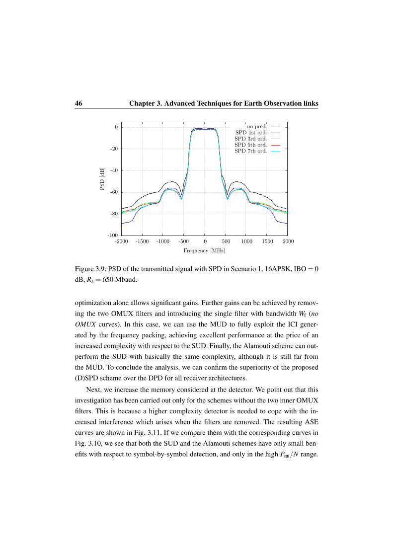
3.9 PSD of the transmitted signal with SPD in Scenario 1, 16APSK,IBO = 0 dB, Rs = 650 Mbaud. . . . . . . . . . . . . . . . . . . . . 46
3.10 ASE for Scenario 2 with L = 0. . . . . . . . . . . . . . . . . . . . . 47
3.11 ASE for Scenario 2 with L = 1. . . . . . . . . . . . . . . . . . . . . 48
3.12 ASE as a function of Rs for the MUD receiver. . . . . . . . . . . . . 49
3.13 ASE and F as a function of Rs for the MUD receiver and Psat/N = 25dB. . . . . . . . . . . . . . . . . . . . . . . . . . . . . . . . . . . . 50
3.14 ASE as a function of Rs for the MUD receiver and PSK constellations. 51
3.15 Packet Error Rate (PER) performance comparison between the sim-ple CS and IC-CS detector, using an 8−PSK with rc = 23/36 atRs = 800MHz. . . . . . . . . . . . . . . . . . . . . . . . . . . . . 52
3.16 PER performance comparison between the simple CS and IC-CS de-tector, using an 16−APSK with rc = 3/4 at Rs = 800MHz. . . . . . 53
4.1 Function Γ(t;ak) for different values of ak in the case SF = 2. . . . . 57
4.2 Function Λ(t;ak) for different values of ak in the case SF = 2. . . . 58
4.3 Continuous part Wc( f ) of the power spectral density of LoRa signalsfor SF = 7 and SF = 12. . . . . . . . . . . . . . . . . . . . . . . . 59
List of Figures v
4.4 Normalized mean square error between signals s(t) and s(t) versusNs for SF = 7 and 12. . . . . . . . . . . . . . . . . . . . . . . . . . 61
4.5 Function Φ(t;ak) for different values of ak in the case SF = 2. . . . 614.6 Function Ψ(t;ak) for different values of ak in the case SF = 2. . . . 624.7 SER for strategies (4.9) and (4.10). . . . . . . . . . . . . . . . . . . 674.8 SER comparison between strategies (4.10) and (4.13). . . . . . . . . 694.9 Instantaneous frequency Γ(t) for the sequence of preamble symbols
in LoRaWAN. . . . . . . . . . . . . . . . . . . . . . . . . . . . . . 704.10 Normalized mean square estimation error for the adopted algorithms
used for the identification of the frequency peaks. The correspondingMCRLB is also reported for comparison. . . . . . . . . . . . . . . . 73
4.11 a) Doppler shift and b) Doppler rate as a function of the distance fromthe satellite projection on the Earth surface. . . . . . . . . . . . . . 75
4.12 PER performance in the presence of Doppler rate, with perfect com-pensation of timing and frequency offset, for SF = 10 on the left andSF = 12 on the right. . . . . . . . . . . . . . . . . . . . . . . . . . 76
4.13 Normalized square root of the MSEE for the four considered algo-rithms. The MCRLB is also reported. . . . . . . . . . . . . . . . . 78
4.14 Normalized square root of the MSEE for increasing number of symbols. 784.15 Overall receiver. . . . . . . . . . . . . . . . . . . . . . . . . . . . . 794.16 PER performance in presence of random impairments (continuous
lines), and with perfect estimation and compensation (dashed lines),for SF = 7÷12. . . . . . . . . . . . . . . . . . . . . . . . . . . . . 82

List of Tables
2.1 Bit indices i in descending order of I(bi;y) for each considered MOD-COD. . . . . . . . . . . . . . . . . . . . . . . . . . . . . . . . . . 28
3.1 Optimized symbol rate Rs (in Mbaud) for the curves in Fig. 3.6. . . 433.2 Details of the ASE in Fig. 3.10 for the DSPD and the MUD receiver. 48
4.1 Normalized distance 1N ‖A− I‖F for different values of SF. . . . . . 63


List of Acronyms
ACM Adaptive Coding and Modulation.
AIR Achievable Information Rate.
APSK Amplitude-Phase Shift Keying.
ASE Achievable Spectral Efficiency.
AWGN Additive White Gaussian Noise.
BCJR Bahl, Cocke, Jelinek and Raviv.
BICM Bit Interleaved Coded Modulation.
CRC Cyclic Redundancy Code.
CS Channel Shortening.
DFT Discrete Fourier Transform.
DPD Data PreDistorter.
FDM Frequency Division Multiplexing.
FFT Fast Fourier Transform.
FS Fractionally Spaced.

x List of Acronyms
HPA High Power Amplifier.
IBO Input Back-Off.
IC Interference Cancellation.
ICI Inter-Channel Interference.
IMUX Input Multiplexer.
IoT Internet of Things.
ISI Inter-Symbol Interference.
LAN Local Area Network.
LDPC Low-Density Parity Check.
LEO Low Earth Orbit.
LLR Log Likelihood Ratio.
LPWAN Low Power-Wide Area Network.
LS Least Squares.
MAP Maximum A Posteriori.
MCRLB Modified Cramér-Rao Lower Bound.
MMSE Minimum Mean Square Error.
MODCOD Modulation/Coding.
MSE Mean Square Error.
MSEE Mean Square Estimation Error.
MUD Multiuser Detector.

List of Acronyms xi
OMUX Output Multiplexer.
PDF Probability Density Function.
PER Packet Error Rate.
PMF Probability Mass Function.
PSD Power Spectral Density.
PSK Phase Shift Keying.
QAM Quadrature Amplitude Modulation.
RF Radio Frequency.
RLS Recursive Least Squares.
RRC Root Raised Cosine.
SER Symbol Error Rate.
SIMO Single Input-Multiple Output.
SNR Signal-to-Noise Ratio.
SPD Signal PreDistorter.
SUD Single User Detector.
TDM Time Division Multiplexing.
TDMA Time Division Multiple Access.
TFP Time-Frequency Packing.


Introduction
Nowadays everything is becoming connected. It is estimated that by the year 2020more than 200 billions of devices will be connected all around the world. This ex-ponential growth requires continuous improvements and more efficient use of theresources for each connection of this huge and complex network.
The focus of this thesis will be on satellite communications. They comprehendmany applications such as high-quality television services, internet connectivity, teleme-try, extension of terrestrial networks and many others. Here, after a short overviewof information theoretic results given in Chapter 1, we will focus on improvementsin reliability, efficiency, and coverage in three different scenarios of satellite commu-nications. Each scenario will be covered in a different Chapter, where we show thedesign of new schemes for transmitters and receivers and analyze their performance.
Broadcast and unicast satellite connections probably represent the most popu-lar scenarios in satellite communications. The information source is on the groundand transmits to a satellite transponder, whose main function is to filter out adjacentchannels, amplify the signal and re-transmit it to the ground towards the receiver. Inbroadcast connections, many receivers will get the same signal (e.g, for televisionservices) while unicast connections are mostly used for Internet coverage in remoteareas. Chapter 2 proposes a solution that could improve speed or reliability in thesescenarios. It is based on the idea that two (or more) neighbor users could cooperateusing a side-channel to exchange information about the received signals and thus,collaboratively, implement a diversity receiver. In fact, the increasing demand forhigh-speed Internet services and high-definition television needs receivers that ex-

2 Introduction
ploit the channel in the best possible way. Moreover, in these days, the widespreadwired and wireless Local Area Network (LAN) could be employed in this context asside-channels. The work is based on the extension of the second generation digitalvideo broadcasting DVB-S2X [1]. Different possible schemes are derived and ana-lyzed. To make it more realistic, we used the hypothesis that the side-channel hasnot an infinite capacity but it is constrained to a maximum fixed information rate thatcould pass through it.
Another important scenario in the field of satellite communications is representedby telemetry. Telemetry means measuring using remote devices, and typical applica-tions are represented by Earth observation and collection of environmental data fromsatellites. In these scenarios, information is thus generated directly on board of satel-lites and then is sent to the ground. In Chapter 3, we carry out an analysis to find asuitable scheme for both transmitters and receivers meant for these applications. Wepropose the use of a signal predistorter between the modulator and the High PowerAmplifier (HPA) to better compensate the effects of amplifier’s non-linearity. Then,we describe improvements in spectral efficiency through optimization of the trans-mission parameters on board of the satellite and discuss on the benefits of advancedlow-complexity receivers.
Internet of Things (IoT) will be among the main contributors to the extremegrowth in the number of connected devices. Different transmission schemes and pro-tocols are used in this context and thus gateways are needed to connect the devices tothe Internet. However, their diffusion showed the necessity to extend coverage in re-mote areas (e.g., to collect data from wildlife or pipeline sensors). Chapter 4 describesa way to use a swarm of Low Earth Orbit (LEO) satellites to help in these scenarios,by relaying the messages intended for the gateway when the devices are located farfrom the urban environments. To remain in the low-orbit (around 700 km above theground), satellites must maintain a very high speed (∼ 7.5 km/s). Thus, Doppler ef-fect is very strong and can be detrimental for a simple transmission scheme that is notmeant to be used on LEO satellites. The study is based on a promising proprietaryIoT protocol called LoRa, designed to be used in terrestrial communications. Themodulation scheme at the physical layer is also proprietary [2] and is slightly differ-

Introduction 3
ent from the traditional modulations found in digital communications textbooks. Wewill describe this spread-spectrum modulation format, its main properties and we willpropose a receiver scheme that could allow the reception of LoRa signals even in thischallenging scenario. The results presented in Chapter 4 do not take into account ef-fects of interference coming from all the different users transmitting in the satellite’sfield of view. However, the interested reader could find details on this discussion in[3].


Chapter 1
Theoretical background
Before the detailed description of the analyzed scenarios and proposed techniques,we present a brief but useful overview of the theoretical background to the resultspresented in the following chapters. The underlying concepts are taken from informa-tion theory. Here we introduce Achievable Information Rate (AIR) and AchievableSpectral Efficiency (ASE) and explain why they are important metrics to measure theperformance of a communication system. We also introduce the mismatched detec-tion and the Channel Shortening (CS) framework. Moreover we show how they canbe useful on a satellite scenario.
1.1 Information rate and mismatched detection
Information theory gives us results about the fundamental limits of communicationsand processing. The building blocks of this subject can be found in [4]. Let us intro-duce the concept of information rate. If we call x a vector of transmitted N symbolsbelonging to a finite alphabet and y a vector of the same length representing the re-ceived symbols, i.e. the symbols passed through the channel, we can define the AIRas
I(x;y) = limN→∞
1NE[
log2p(y|x)
∑x′ p(y|x′)P(x′))
][bits / ch.use]. (1.1)

6 Chapter 1. Theoretical background
The operator E[·] represents the expectation operator, P(x) is the Probability MassFunction (PMF) of the channel inputs and p(y|x) is the Probability Density Func-tion (PDF) that describes the channel. Thus the AIR is linked both to the choice ofthe transmitted symbols through the PMF p(x) and to the channel through the PDFp(y|x). It can be interpreted as the average mutual information per transmitted sym-bol and thus represents the maximum amount of information bits per each transmittedsymbol that can be reliably sent on the channel with the selected input alphabet.
Let us consider a simple channel described by the following equation,
y = Hx+w, (1.2)
where H is a Toeplitz matrix representing the Inter-Symbol Interference (ISI) intro-duced by the channel and w is a vector whose elements are complex Additive WhiteGaussian Noise (AWGN) samples, with mean zero and variance N0.
Computing the AIR in closed form through (1.1) is not a straightforward opera-tion. However, using the Monte Carlo method described in [5], we can compute theAIR numerically since we have available the optimal Maximum A Posteriori (MAP)symbol detector for this kind of channel. This optimal detector is based on the Bahl,Cocke, Jelinek and Raviv (BCJR) algorithm [6]. The BCJR will be based on thechannel PDF,
p(y|x) = 1(πN0)N exp
(−‖y−Hx‖2
N0
)
=1
(πN0)N exp
(−y†y−2ℜ
{y†Hx
}+x†Gx
N0
), (1.3)
where we introduced the matrix G = H†H. However, the feasibility of the MAP de-tector depends on the length L of the memory introduced by the channel through thematrix H. In fact, calling M the cardinality of the alphabet, the BCJR detector’s com-plexity is O
(ML)
or, in other words, it depends exponentially on L. Moreover, wecannot always fully describe the channel in the simple form of (1.2). For the sake ofexample, the satellite channel typically includes a nonlinear transponder.
We can now introduce the mismatched detection principle described in [7]. Infact, we can think of an auxiliary channel described by the PDF q(y|x) for which

1.2. Channel Shortening 7
an optimal detector is feasible. Then, we can compute through the algorithm [5] thequantity,
Iq(x;y) = limN→∞
1NE[
log2q(y|x)
∑x′ q(y|x′)P(x′))
]. (1.4)
This will be computed using the output y of the actual channel but employing adetector based on the auxiliary channel PDF q(y|x). As demonstrated in [7], Iq(x;y)will be a lower bound to I(x;y), but it will be also achievable by that detector. Thismeans that we are capable of numerically compute the AIR that will depend on theinput constellation, on the channel, and the detector based on q(y|x). The detectorwill be thus optimal for the auxiliary channel but sub-optimal for the actual channel.The next step will be understanding how to properly choose the auxiliary channelthrough the CS technique.
1.2 Channel Shortening
To design a receiver with a reasonable complexity, many approaches have been pro-posed. We can think of two basic types of algorithms: one that selects only a fractionof the trellis to explore (see [8], [9] and [10]) and the other that builds a reduced trellisto be fully explored (e.g., [11]). We describe here the Channel Shortening techniqueproposed in [12], that belongs to the second kind of algorithms. It is based on thechannel model (1.2) and, even though it is designed under the hypothesis of Gaussianinputs x, it works also on finite cardinality alphabets.
The first step consists of choosing the memory of the reduced complexity detec-tor ν ≤ L. Then, the algorithm computes the matrices Hr and Gr to be used in themismatched detector based on the following auxiliary channel model
q(y|x) ∝ exp(−y†y−2ℜ
{y†Hrx
}+x†Grx
).
The computation of Hr and Gr is the result of a maximization of a lower bound tothe information rate, differently from other works on the subject that performed anoptimization of the Minimum Mean Square Error (MMSE) [11]. The elements of the

8 Chapter 1. Theoretical background
Gr matrix must satisfy the constraint {Grmn}= 0 for |m−n|> ν . For ISI channels Gr
and Hr are Toeplitz matrices completely characterized by the discrete-time sequencesgr
k e hrk. Let us call Gr(ω) and Hr(ω) the Fourier transform of those sequences. Then,
we can compute
Hr(ω) =H∗(ω)
|H(ω)|2 +N0(Gr(ω)+1).
and Gr(ω) can be found through the following factorization,
Gr + I = UU†
where U is an upper triangular matrix. Defining,
A(ω) =N0
|H(ω)|2 +N0(1.5)
and its inverse Fourier transform ak, we can build the Toeplitz matrix
Aν =
a0 . . . aν−1...
. . ....
a−(ν−1) · · · a0
.
and the vector aν = [a1 · · ·aν ]. It can be shown that the elements of matrix U can beobtained through the following equations
u0 =1√
a0−aν(Aν)−1a†
uν =[u0,−u0aν(Aν)−1] .
CS is a very general framework and it is possible to demonstrate that for the simplestcase of ν = 0 it collapses into an unbiased version of MMSE receiver, while it rep-resents the optimal detector for ν = L. In [13] and [14], the CS has been extended toreceivers that perform iterative detection and decoding. At each iteration, the filtersare updated based on the quality of the soft-decision and the soft-symbols are em-ployed to perform an Interference Cancellation (IC). In this IC-CS the soft-symbols

1.3. Spectral efficiency and Time-Frequency Packing 9
are filtered by a filter R(ω) and subtracted to the received samples. R(ω) can be foundthrough an iterative algorithm, since no closed-form solution can be found for it.
Both these reduced complexity receivers need to know the channel matrix H.The work performed in [15], instead, shows a way to implement the first version ofCS in an adaptive scenario. It is shown that A(ω) in (1.5) is just the Power SpectralDensity (PSD) of the MMSE sequence ek = yMMSEk− xk, where {yMMSEk} are thereceived samples after an MMSE filter. It also shows that introducing the MMSEfilter HMMSE(ω), Hr(ω) can be factorized as,
Hr(ω) = HMMSE(ω)(Gr(ω)+1).
So the CS receiver could be employed after an adaptive MMSE filter. This can becomputed trough a Least Squares (LS) or Recursive Least Squares (RLS) algorithm[16]. Then, by the error sequence ek we can compute Aν and a since,
ak =1
N− k
N−k−1
∑i=0
ei+ke∗i .
Similarly, also the IC-CS receiver could be implemented in an adaptive fashion,but with some degrees of approximation. In fact, while the CS needs only the first ν+
1 taps of bk, the IC-CS needs the full PSD B(ω). So, in a practical implementation,we can use the estimated bk taking taps until bk is small enough to be negligible. Theadaptive version of the CS is useful on many satellite scenarios since the channelis not given in a simple closed form due to nonlinear distortions coming from thesatellite amplifiers. In fact, a nonlinear HPA is present on board of a satellite (seeChapter 2 and Chapter 3).
1.3 Spectral efficiency and Time-Frequency Packing
Even though AIR seems a good metric to judge the amount of information that canbe sent through a given channel, it gives no information about how efficiently weare exploiting the channel resources. In fact, we could reach a good performancebut maybe using too much of the time and frequency resources. That is why we

10 Chapter 1. Theoretical background
introduce the ASE, taking into account also the amount of occupied bandwidth Wand the symbol period Ts
ASE =I(x;y)WTs
[bit/s/Hz] . (1.6)
This idea leads to the concept of Time-Frequency Packing (TFP) [17]. In fact, ifwe occupy less bandwidth W (e.g., through tighter filters) and transmit more rapidly(smaller Ts), we are giving up orthogonality and we are introducing some degrees ofISI and Inter-Channel Interference (ICI). This could lead to a smaller AIR but sincewe are also decreasing the product WTs, there is a possible efficiency improvement foran appropriate choice of WTs. Of course, depending on the channel and on the amountof introduced memory, the optimal receiver could quickly become unfeasible. So, weuse the achievable lower bound Iq(x;y) instead of the optimal I(x;y) to computethe ASE in (1.6). Also, we employ the CS framework since it optimizes the AIRfor a fixed complexity constraint. This technique led to significant improvement indifferent scenarios like in wireless [18], optical [19], and also satellite links [20].

Chapter 2
Cooperative Receivers Through aConstrained Link
The always increasing demand for high-speed Internet services and high-definitiontelevision needs receivers that exploit the channel in the best possible way. Moreover,in these days, both wired and wireless LAN are widespread. In this Chapter, we study,from a physical layer perspective, a scheme where satellite receivers exploit a LAN(just for the sake of an example, but could be any other kind of link), as a way toexchange information and thus, collaboratively, implement a diversity receiver. Thestandard on which the study is performed is the extension of the second generationdigital video broadcasting DVB-S2X [1]. In the ideal case of infinite backhaul capac-ity, assuming the same channel model but with different noise process realizations,we could achieve a 3 dB gain with just two cooperating receivers. In fact, a simplereceiver should only need to average out the noise by coherently summing the tworeceived signals. However, we analyze the performance of a scheme where the capac-ity of the cooperation link is constrained to a fixed rate per channel use. Thus, one ofthe receivers needs to suitably compress its signal before sending it to the other user;in this Chapter we assume the simplest possible solution where the helping user ismerely quantizing its signal, in order to reduce the complexity burden for the helpinguser as much as possible. This scheme could also be applied to cooperation among

12 Chapter 2. Cooperative Receivers Through a Constrained Link
many users.The application scenarios are multiple. An example could be for broadcasting.
Users at the edge of a coverage area could cooperate to have more reliable or im-proved service. In a unicast scenario for Internet connection, where a Time DivisionMultiple Access (TDMA) is employed, the users could cooperate by turn: each user,during its idle time-slots, could receive the signal meant for the other and then sendthe quantized version. Thus, the gains in Signal-to-Noise Ratio (SNR) could be ex-ploited by the Adaptive Coding and Modulation (ACM) scheme to have improvedconnections.
The idea of taking advantage of a constrained backhaul link has already been pro-posed and applied to the base stations of a cellular system (see, e.g., [21]). We insteadadopt it to synthesize satellite receiver cooperation, where the complexity constraintcan be tighter. Moreover, as a performance metric, we take a lower bound to the in-formation rate of the cooperative receiver, based on the joint distribution of the fullversion and the quantized version of the signal, rather than just the information rateof the quantized signal alone. The computation of the information rate will be basedon the Monte Carlo method described in [5].
In this chapter, we will first describe the reference receiver, the employed chan-nel model and the assumptions on which our work is based. Then, we will give adescription of different approaches for receivers and quantization schemes and wereport, and comment upon, the results in terms of mutual information and PER forthe different approaches.
2.1 Employed channel models
2.1.1 Reference model
The channel we are studying is the single-carrier per transponder satellite channel,where the DVB-S2X standard is employed. The information bits are generated andencoded in the gateway. The channel coding is the Low-Density Parity Check (LDPC)foreseen by the standard. The bits are then interleaved, mapped to complex symbolsand finally sent to a satellite transponder. The complex envelope of the signal output

2.1. Employed channel models 13
w(t)
s(t) r(t)HPAIMUX OMUX
Satellite transponder∑k xkp(t− kT )
Figure 2.1: Block diagram of the satellite transponder.
from the Earth gateway is thus,
x(t) = ∑k
xk p(t− kTs).
The complex symbols xk belong to Amplitude-Phase Shift Keying (APSK) con-stellations, as defined in the DVB-S2X standard [1, 22], while Ts is the symbol inter-val, p(t) a Root Raised Cosine (RRC) pulse with roll-off factor β and signal band-width W = (1+ β )/T . The values of β and W have been chosen according to theoptimization performed in [23], and thus set to β = 0.05 and a baud rate Rs =
1T = 37
Mbaud.The transponder is composed of an Input Multiplexer (IMUX) filter to remove
adjacent channel interference, a HPA that introduces non-linear distortions and anOutput Multiplexer (OMUX) to reduce the spectral regrowth due to the HPA. TheHPA is modeled as a memoryless non-linearity defined by its AM/AM and AM/PMcharacteristics. The IMUX and OMUX filters have 3 dB bandwidths of WIMUX = 42MHz and WOMUX = 38 MHz respectively. Their frequency responses are shown inFig. 2.2 and 2.3 while HPA’s AM/AM and AM/PM characteristics can be found inFig. 2.4 (see also [22]).
We point out that x(t) is modeled as noiseless and noise is taken into account asAWGN between the transponder and the receiver. A block diagram is depicted in Fig.2.1.
The front-end of the receiver is based on a Fractionally Spaced (FS) MMSE de-tector [24] with oversampling factor η = 2. The received signal r(t) is first filteredby a low-pass front-end with a bandwidth sufficiently large to permit the subsequent

14 Chapter 2. Cooperative Receivers Through a Constrained Link
−70
−60
−50
−40
−30
−20
−10
0
−40 −20 0 20 40
Rejection
[dB]
Frequency [MHz]
Figure 2.2: IMUX frequency response.
−45
−40
−35
−30
−25
−20
−15
−10
−5
0
−40 −20 0 20 40
Rejection
[dB]
Frequency [MHz]
Figure 2.3: OMUX frequency response.

2.1. Employed channel models 15
−16
−14
−12
−10
−8
−6
−4
−2
0
−20 −15 −10 −5 0 5−10
0
10
20
30
40
50
60
70
OutputPow
er[dB]
OutputPhase[D
eg]
Input Power [dB]
Output PowerOutput Phase
Figure 2.4: HPA AM/AM and AM/PM characteristics.
oversampling at a sampling rate ηRs [25]. Then, after FS-MMSE filtering and down-sampling, we obtain the samples yk where k is the symbol time index.
To mitigate the effects of HPA non-linearity, a memoryless Data PreDistorter(DPD) [26] is used at the transmitter, together with a certain amount of Input Back-Off (IBO) which depends on the cardinality of the constellation [27]. We also pointout that perfect synchronization at the receiver is assumed.
Within satellite communications, it is customary to define the SNR as Psat/N,where Psat is the saturation power of the HPA, while N is the noise power over theOMUX bandwidth. This is related to Es/N0 as,
Psat
N=
Es
N0
Rs
WOMUXOBO,
where OBO stands for the output back-off of the HPA.
2.1.2 Cooperation between terminals
We employ a matrix formulation, so that, e.g., the transmitted symbols are repre-sented with the vector x = [x1, · · · ,xN ]
T where N is the number of transmitted sym-

16 Chapter 2. Cooperative Receivers Through a Constrained Link
bols.
We analyze a scheme with two users that are physically close and can receive, inthe absence of noise, the same signal s1(t). User 2 is helping user 1 through a side-channel with a capacity bc bits per symbol time. For the sake of simplicity, we con-sider an error-free side-channel and a negligible delay. See Fig. 2.5 for an overview
of the analyzed scenario. We denote by y(i) =[y(i)1 , · · · ,y(i)N
]Tthe vector containing
the digital samples received by user i. The subscript k in y(i)k is the symbol time indexand sampling is done in the same way as in the reference scheme. The channel modelis based on the assumption that the signals received by the two users are affected bythe same ISI and have the same channel gains, but it is straightforward to extend themodel to include different channels. However, our assumption is reasonable when-ever the two users are physically close. The channel is represented by an N×N matrixH. The number of rows and columns should actually be different to take into accountthe channel tails, but this is irrelevant asymptotically as N grows without bounds andsimplifies the notation. The signals are also affected by two independent AWGN pro-cesses n1,n2 ∼ CN (0,N0I). Since the side-channel is constrained in capacity to bc
bits per channel use, we need a lossy compression of y(2) to reduce its entropy. Weopted for a quantization of the signal y(2), where each element y(2)k is quantized toa set Q with cardinality |Q| = 2bc , through a quantizer q : C→Q. The quantizedversion of y(2) will be represented as y(2). The system as seen by user 1 (i.e., the userthat is receiving a quantized version of the same signal, but with another noise re-alization), can be modeled as a non-linear Single Input-Multiple Output (SIMO)-ISIchannel:
[y(1)
y(2)
]=
[y(1)
q(y(2))
]=
[Hx+n1
q(Hx+n2)
].
So, we should design a proper scalar quantization function q(·) and a receiverscheme to maximize the mutual information based on the joint distribution of (y(1), y(2)),namely I(x;y(1), y(2)), that can be computed as,

2.1. Employed channel models 17
Figure 2.5: Simplified scheme of the analyzed system. The same signal, but withdifferent noise realization, is received by both users. Then user 2 send a quantizedversion of its signal to user 1 through a constrained link.
I(x;y(1), y(2)) =
limN→∞
Ep(y(1),y(2),x)
[log2
p(y(1),y(2),x)p(y(1),y(2))p(x)
]
N. (2.1)
The information transfer can be represented by the Markov chain x→ (y(1),y(2))→(y(1), y(2)). Rate distortion theory [4] could be helpful to find an optimal quantizationscheme from an information rate perspective, since it minimizes a certain distortionmetric given a target rate. However, the techniques studied in this field are usuallyworking with a quantization of signals not affected by noise. We are instead quan-tizing the noisy signal y(2) coming from the noiseless source x. Thus, optimizing theinformation transfer in y(2) → y(2), neglecting that the actual information source isx, is not guaranteed to optimize the whole information transfer x→ y(2)→ y(2) [28].Also, the distortion function is minimizing a distance (typically Euclidean distance)between the quantizer’s inputs and outputs but, as we will see in the following sec-tions, the quantization scheme with better gains does not always need to minimizethis distance.

18 Chapter 2. Cooperative Receivers Through a Constrained Link
We also point out that computation of information rate is not possible in closedform for the satellite channel, and we will thus compute it by the Monte Carlo basedalgorithm from [5]. So, choosing a proper q(·) and a proper receiver to optimize (1) isa tough problem to treat mathematically in closed form. We will thus try heuristic ap-proaches that make use of low-complexity schemes both for the quantization schemeand the receiver design, to avoid much computational load for this kind of devices.
2.2 Proposed solutions
2.2.1 MMSE approach
The quantized symbols are y(2) = q(y(2)). We can model them as,
y(2) = y(2)+n2 +nq,
where nq is the noise due to quantization. So the channel seen by user 1 becomes,
y =
[y(1)
y(2)
]= Htx+
[n1
n2 +nq
],
where Ht =
[HH
]is a 2N×N block matrix. Both in this and in the following sub-
section we employ a simple quantization scheme, based on equally spaced symbolsbelonging to square or non-square Quadrature Amplitude Modulation (QAM), for aneven or odd number of quantization bits respectively.
The receiver will be based on an extension of the unbiased linear MMSE receiver[29] for SIMO-ISI channels. Let us introduce HMMSE, which is an N × 2N matrixrepresenting the MMSE filter. Then we define yMMSE = HMMSEy as the N×1 vectorat the output of the MMSE filter and the MMSE bias α , which can be computed as afunction of the Mean Square Error (MSE) α = 1−E
[|yMMSEk− xk|2
]. The unbiased
receiver needs to implement a symbol by symbol receiver based on,
xk = argminxk|yMMSEk−αxk|2. (2.2)

2.2. Proposed solutions 19
To deal with the quantization noise, that is not a white Gaussian process and is notguaranteed to be uncorrelated with the information symbols, we keep a more generalnotation based on covariance matrices rather than on channel matrix H and noisepower spectral density N0. The covariance matrices are defined as,
Cxy = E[(x−E [x]) (y−E [y])†
]
Cyy = E[(y−E [y]) (y−E [y])†
].
We start computing the MSE matrix, that is needed to compute the bias α . TheMSE matrix is,
A = E[(yMMSE−x)(yMMSE−x)†
]
=−CxyC−1yy C†
xy + I, (2.3)
where I is the identity matrix, representing Cxx under the assumption of unit energyand uncorrelated transmit symbols.
We can now notice how these covariance matrices can be expressed as blockmatrices of the form,
Cxy = E[xy†]=
[Cxy(1) Cxy(2)
]
Cyy = E[yy†]=
[Cy(1)y(1) Cy(1)y(2)
C†y(1)y(2)
Cy(2)y(2)
],
where Cxy(1) , Cxy(2) , Cy(1)y(2) are square N×N Toeplitz matrices.
To simplify the notation, we resort to Szego’s Theorem applying spectral decom-position to these block matrices. Asymptotically as N→∞, we can equivalently workwith the Fourier transform of the sequence associated with each Toeplitz matrix. De-noting the N×N Fourier matrix by Q and the Fourier transform of a square matrix Cby C = Q†CQ, we can write,

20 Chapter 2. Cooperative Receivers Through a Constrained Link
Lxy = Q†Cxy
[Q 00 Q
]=[
Cxy(1) Cxy(2)
]
Lyy =
[Q† 00 Q†
]Cyy
[Q 00 Q
]=
[Cy(1)y(1) Cy(1)y(2)
C†y(1)y(2)
Cy(2)y(2)
],
where all the C are diagonal matrices and each diagonal is the Fourier transform ofa covariance sequence. For the sake of example, Cxy(1) has as diagonal the Fouriertransform function Cxy(1)(ω), whose inverse-transform is the covariance sequencecxy(1) defined by its elements,
cxy(1)k
= E[xly
(1)l+k
].
We also make use of bold notation (e.g., Lyy(ω)) to describe a matrix of functionsdepending on the angular frequency ω . In such a way, the diagonal form allows usto carry out the inversion in (2.3) straightforwardly using the block matrix inversionformula,
L−1yy (ω) =
[Cy(2)y(2)(ω) −Cy(1)y(2)(ω)
−C†y(1)y(2)
(ω) Cy(1)y(1)(ω)
]
Cy(1)y(1)(ω)Cy(2)y(2)(ω)−|Cy(1)y(2)(ω)|2 (2.4)
and thus A(ω), the Fourier transform associated to (2.3), is,
A(ω) =|Cxy(1)(ω)|2Cy(2)y(2)(ω)+Cy(1)y(1)(ω)|Cxy(2)(ω)|2
Cy(1)y(1)(ω)Cy(2)y(2)(ω)−|Cy(1)y(2)(ω)|2 (2.5)
−2ℜ
{Cxy(1)(ω)Cy(1)y(2)(ω)C†
xy(2)(ω)}
Cy(1)y(1)(ω)Cy(2)y(2)(ω)−|Cy(1)y(2)(ω)|2 .
We can now call a the inverse-transform of A(ω) and express the bias α in (2.2) as,
α = 1− 12π
∫π
−π
A(ω)dω = 1−a0.

2.2. Proposed solutions 21
The MMSE filter is,
HMMSE = CxyC−1yy = [ HMMSE1 HMMSE2 ].
Defining the denominator of A(ω) as a function D(ω) = Cy(1)y(1)(ω)Cy(2)y(2)(ω)−|Cy(1)y(2)(ω)|2, and by applying the spectral decomposition,
HMMSE(ω) = Lxy(ω)L−1yy (ω),
we can express the MMSE filter in the Fourier domain as,
HMMSE1(ω) =Cxy(1)(ω)Cy(2)y(2)(ω)−Cxy(2)(ω)C†
y(1)y(2)(ω)
D(ω)
HMMSE2(ω) =Cxy(2)(ω)Cy(1)y(1)(ω)−Cxy(1)(ω)Cy(1)y(2)(ω)
D(ω).
In this form, this receiver is very convenient when we do not have a closed formof the channel because we can simply perform an estimation of the cross and self-covariance sequences. This is the case for the satellite channel and the quantizedchannel, where the non-linearity comes into play and we need an estimate of theircovariance structure. It needs to be pointed out that the unbiased MMSE filteringstrategy is very general, since it still applies in case of different channels or differentSNRs for user 1 and 2 since only the covariances need to be estimated.
The use of the asymptotic properties of these block matrices simplifies the in-version procedure in (2.4). In fact, instead of computing the inverse of a 2N × 2Nmatrix, we switched to the simplified case of a 2×2 matrix. Thus, it is also possibleto use this algorithm in an extended version. Assuming U−1 helping users, we havean UN×UN matrix to be inverted. After the transformation to the Fourier domain,we obtain a matrix with dimension U×U where each element is a function of ω , andthe inverse could be computed as,
C−1yy (ω) =
adj(Cyy(ω))
det(Cyy(ω)).

22 Chapter 2. Cooperative Receivers Through a Constrained Link
Having a closed form of A(ω) in (2.5) is also useful for channels with a strongerISI. As explained in Chapter 1, we could easily employ the CS technique since A(ω)
is the only thing needed to compute the CS filter and the reduced trellis. So, thisreceiver can be easily extended to channels with much more memory, where a BCJRreceiver with memory L > 0 can give higher performance improvements.
2.2.2 BCJR modifications
The BCJR detector [6] is based on the transition probabilities p(yk|xk,σk), wherethe state σk for an ISI channel with memory L is σk = (xk−1, · · · ,xk−L). In our case,user 1 must base the trellis on p(y1k , y2k |xk,σk) = p(y1k |xk,σk)p(y2k |xk,σk), where weexploited the conditional independence of y1k and y2k given the channel inputs. So,while p(y1k |xk,σk) remains unaltered in the presence of a helping user, we need toaccommodate for p(y2k |xk,σk), which is very hard to compute in the general case:
p(y2k |xk,σk) =∫
Rp(y|xk,σk)dy
=∫
R
1πσ2 exp
{ |y−∑Ll=0 hlxk−l|2σ2
}dy
where R = {y ∈ C : q(y) = y2k}.If the channel impulse response hl is real-valued, then it is possible to exploit the
independence of the real and complex part to obtain two separate integrals. More-over, in case of a uniform quantization function, the integrals could be expressedas differences of Q-functions. However, on satellite channels, the above-mentionedsimplifications are not exploitable due to the presence of non-linear HPAs. Anyway,regardless of the way p(y2k |xk,σk) values are calculated, in a real implementationthey can be precomputed and stored in a look-up table. We also point out that thisscheme is based on the Forney channel model [30] for the probabilities describingthe quantized channel, while a closed form solution based on Ungerboeck model[31] is hard to derive.
In the next section, we resort to a simple estimation of the probabilities p(y2k |xk,σk).However, even with a small memory, this estimation process can quickly become pro-
2.2. Proposed solutions 23
hibitive. If the effects of the channel memory are not too strong, we could thus employan MMSE filter before quantization. In such a way, the channel state to be taken intoaccount is only one and we can just estimate p(y2k |xk) without a significant loss inperformance. This is applicable to the satellite channel. Even with the signal baudrate optimization as performed in [24, 32], having Rs = 37 MBaud, it is possible tosee that the introduced memory is negligible. In fact, there is no gain in resorting toa higher memory detector [24].
That being said, this model also remains a valid approximation for any kind ofISI channel and the computed mutual information is achievable since it is an optimaldetector for an auxiliary channel [33, 5].
2.2.3 LLR quantization
Since we are interested in the coded performance of the system, one could ask whatcould be done to focus the information on some bits. The answer is working on quan-tizations of the bits’ Log Likelihood Ratio (LLR). For a given Modulation/Coding(MODCOD) scheme, we could thus focus the information we are sending only onsome selected bits of the constellation.
A couple of important remarks are in place. This approach is not guaranteed tobe optimal, especially when iterative detection and decoding schemes are performed.It can be, however, optimal when an iterative receiver cannot be employed, as statedby the Bit Interleaved Coded Modulation (BICM) principle [34]. Let us define asbk,i the ith transmitted bit belonging to the kth symbol. Then, we introduce the vectorb = [b1,1 · · ·b1,log2 M · · ·bN,1 · · ·bN,log2 M]T and bi = [b0,i · · ·bN,i]
T . We point out thati is thus not a temporal index and is 1 ≤ i ≤ log2 M. We aim at maximizing Cb =
∑i I(bi;y(1), y(2)), the sum of mutual information between the received signals andthe ith bits of each symbol. Cb is an achievable lower bound to I(x;y(1), y(2)) since,
I(x;y(1), y(2)) = I(b;y(1), y(2))≥∑i
I(bi;y(1), y(2)),
and it is strongly influenced by the bit-mapping function.We remain with a degree of freedom: the decision on which bits to improve the
LLRs of. One could argue that helping the weakest ones first (i.e., the ones with

24 Chapter 2. Cooperative Receivers Through a Constrained Link
lowest I(bi;y(1)) for a given SNR) should be the best approach. Actually, we shoulddecide for the bits with the highest slope ∂ I(bi;y(1))
∂SNR . It is thus not guaranteed in thegeneral case that helping the weakest bit first is the best thing to do.
However, we are focusing our attention on high-order modulation schemes forsatellite channels. It is easy to argue that for the values of efficiency aimed by theseMODCODs, the mutual information will be well above 0 for all values of i. Thismeans that the major constraint for the decoding process will be represented by theweakest bits, since the strongest ones will be near the saturation point of the curve.In Figs. 2.6a, 2.6b, and 2.6c, the values of I(bi;y(1)) and I(x;y(1)) are reported forthe MODCODs 16, 32, and 64-APSK with a code rate rc = 3/4, 3/4, and 4/5, re-spectively, on a satellite channel with no cooperation and MMSE detector. It is alsohighlighted the point where I(x;y) = rc log2 M to let the reader understand the SNRregion where they are going to be used. If we instead had to work at low SNR (inrelation to the code rate and modulation order), giving information about the weakestbits could have added nothing due to the lower slope of the curve in that region.
Moreover, at high SNRs we could resort to Max-Log-MAP detector, since theapproximation in the computation of the LLR will be almost negligible. This meansthat less computational complexity will be required by user 2.
The adopted quantization scheme is the following: user 2 will compute and thenquantize the LLRs associated to each sequence bi with bLi bits, with the constraint setby the side-channel ∑i bLi = bc. A value bLi = 0 means that no information about bi
will be sent. The quantization thresholds are tailored on estimates of the LLRs distri-butions so that the quantized levels for each bi are equally distributed. Regarding thereceiver of the user 1, it performs an estimate of the probabilities p(y2k |xk) similarlyto the receiver described in Sec. 2.2.2.
We found that whenever bLi ≤ 1 for every position i, a simpler and equivalent ap-proach to design the quantization is clustering based on the MODCOD bit-mapping.We can, in fact, assign a value to y(2)k by grouping symbols that share the same valueof the bits we are intending to help. Examples for the 16-APSK with rc = 3/4, 32-APSK with rc = 3/4, and 64-APSK with rc = 4/5 are reported in Fig. 2.7, 2.8, and2.9, respectively, for bc = 2. We grouped the symbols using the the weakest bits for

2.2. Proposed solutions 25
0
0.5
1
1.5
2
2.5
3
3.5
4
−5 0 5 10 15 20 25 30
Mutualinform
ation[bit/ch.use]
Psat/N [dB]
I(y;x)I(y; b0)I(y; b1)I(y; b2)I(y; b3)
(a) 16-APSK rc = 3/4
0
0.5
1
1.5
2
2.5
3
3.5
4
4.5
5
−5 0 5 10 15 20 25 30
Mutualinform
ation[bit/ch.use]
Psat/N [dB]
I(y;x)I(y; b0)I(y; b1)I(y; b2)I(y; b3)I(y; b4)
(b) 32-APSK rc = 3/4
0
1
2
3
4
5
6
−5 0 5 10 15 20 25 30
Mutual
inform
ation[bit/ch.use]
Psat/N [dB]
I(y;x)I(y; b0)I(y; b1)I(y; b2)I(y; b3)I(y; b4)I(y; b5)
(c) 64-APSK rc = 4/5
Figure 2.6: Mutual Information I(x;y(1)) and I(bi;y) of the reference receiver for theanalyzed MODCODs. We also highlighted the point where I(x;y(1)) = rc log2 M.

26 Chapter 2. Cooperative Receivers Through a Constrained Link
Figure 2.7: Decision regions for 2-bit quantization of the 16-APSK rc = 3/4. Samecolor means same quantized symbol. This approach is intended to help the first twobits (the weakest ones).
each scheme. It is interesting since this mapping seems effective even though it doesnot minimize the MSE distance between quantization inputs and outputs.
2.3 Results
We show the possible gains achievable with the schemes mentioned above. The gainsin SNR of the Cb function with LLR quantization scheme (LLR in the legend) arereported in Figs. 2.10a, 2.10b, and 2.10c, together with the employed bLi values.We employed all possible configurations of [bL0 , · · ·bLlog2 M ], where bLi takes valueof 0, 1 or 2 bits, but we show only the configurations maximizing the gain for agiven bc. In Tab. 2.1 we report the bit indices i ordered by the value I(bi;y) at theSNR where I(x;y) = rc log2 M. Indices sharing the same I(bi;y) value are reportedtwice and separated by a comma. Looking at Tab. 2.1 we see that Fig. 2.10 tends tofollow the foreseen trend of helping the weakest bits. We checked that when it is not,the difference is just on the second decimal digit and could be related to numerical

2.3. Results 27
Figure 2.8: Decision regions for 2-bit quantization of the 32-APSK rc = 3/4. Samecolor means same quantized symbol. This approach is intended to help the first andlast bit (the weakest ones).
Figure 2.9: Decision regions for 2-bit quantization of the 64-APSK rc = 4/5. Samecolor means same quantized symbol. This approach is intended to help the fourth andfifth bit (the weakest ones).

28 Chapter 2. Cooperative Receivers Through a Constrained Link
approximations. For the sake of comparison, we also reported the gains in SNR forthe Cb function with the MMSE receiver and the receiver with modification of BCJRthat performs an estimate of the probabilities (PE in the figures). We decided to useCb as a metric for all of the schemes in order to have a fair comparison. It can be seenthat if the number of quantization bits is lower than log2 M, the LLR scheme seemsmore convenient.
In Figs. 2.11a, 2.11b and 2.11c we show packet error rate (PER) curves for thethree analyzed MODCODs with bc = 2. The gains over the non-cooperative receiverperformance match almost exactly those foreseen by the mutual information (thelimit set by Cb is also reported in the figure).
Table 2.1: Bit indices i in descending order of I(bi;y) for each considered MODCOD.1st 2nd 3rd 4th 5th 6th
16-APSK 3/4 4,3 4,3 2,1 2,1 - -
32-APSK 3/4 4,3 4,3 2 5 1 -
64-APSK 4/5 1,3 1,3 6,2 6,2 5,4 5,4
2.4 Conclusions
In this chapter, we proposed a new scheme for exploiting constrained cooperation insatellite receivers. The constraint is in the capacity of the link between the receivers,where the signal should be quantized. We demonstrated its effectiveness with threedifferent schemes on satellite channels with high order APSK modulation: an MMSEbased approach, an approach based on BCJR modifications and a third one based onLLRs quantization. We also saw that the algorithm that works on the quantized ver-sion of LLRs has higher gains when the number of quantization bits is lower than thenumber of bits necessary to represent all the modulation symbols and that there’s asimple approach to cluster together symbols and design a quantization scheme whenthe number of quantization bits is bc < log2 M. For channels with higher memory,however, the estimation described in Sec. 2.2.2, has a number of probabilities to es-

2.4. Conclusions 29
(a) 16-APSK rc = 3/4 (b) 32-APSK rc = 3/4
(c) 64-APSK rc = 4/5
Figure 2.10: Gains over the reference scenario in SNR for Cb curves achieved by thedifferent schemes.

30 Chapter 2. Cooperative Receivers Through a Constrained Link
10−4
10−3
10−2
10−1
100
11 11.5 12 12.5 13
Cb
PER
Psat/N [dB]Ref. LLR MMSE Prob. Est.
(a) 16-APSK rc = 3/4
10−4
10−3
10−2
10−1
100
14.8 15 15.2 15.4 15.6 15.8 16 16.2 16.4
Cb
PER
Psat/N [dB]Ref. LLR MMSE Prob. Est.
(b) 32-APSK rc = 3/4
10−4
10−3
10−2
10−1
100
19.6 19.8 20 20.2 20.4 20.6 20.8 21 21.2 21.4
Cb
PER
Psat/N [dB]Ref. LLR MMSE Prob. Est.
(c) 64-APSK rc = 4/5
Figure 2.11: PER curves for the analyzed MODCODs and bc = 2. The vertical dashedlines mark the achievable information rates in term of Cb. The PER curves of thereference scheme with no cooperation are also reported for comparison purposes.

2.4. Conclusions 31
timate exponential in the memory of the detector. This means that also the trainingphase for their estimation will be exponentially longer. The LLR-estimation in Sec.2.2.3, instead, would have the drawback of requiring the helping user to perform adetection with a more complex and slow BCJR with L ≥ 1. This would introducemore delay in the system and goes against the principle of minimizing the computa-tional demand for the helping user. The MMSE receiver in Sec. 2.2.1, instead, couldeasily be extended to higher memory channels through the CS framework.


Chapter 3
Advanced Techniques for EarthObservation links
In this chapter, we will apply TFP techniques and more sophisticated receiver archi-tectures to high rate telemetry systems. In this kind of systems, data are generateddirectly on the satellite and then transmitted to Earth. This allows the use of a signalpredistortion algorithm [35, 36, 37], which is expected to better compensate the non-linear effects introduced by the satellite channel with respect to simpler constellationpredistortion techniques used in DVB-S2.
This scenario was the object of an activity promoted by the European SpaceAgency with the aim of introducing possible improvements to the current high ratetelemetry standard [38]. We will analyze two different scenarios, with one and twochannels, respectively. For both scenarios, we will apply advanced techniques at thetransmitter and at the receiver.
3.1 System Model
3.1.1 Single Channel Scenario
The first analyzed scenario, referred to as Scenario 1 in the following sections, is thatdepicted in Fig. 3.1. The information bits to be transmitted to Earth are mapped on

34 Chapter 3. Advanced Techniques for Earth Observation links
w(t)
MOD HPA OMUX
Satellite
s(t) r(t)x(t) z(t)
Figure 3.1: Block diagram of the transmitter for Scenario 1.
K symbols of an M−ary zero-mean complex constellation to generate the sequence{xk}K−1
k=0 . We can express the complex envelope of the transmitted signal as
x(t) =K−1
∑k=0
xk p(t− kTs) , (3.1)
where the shaping pulse p(t) is a RRC pulse with roll-off factor β and Ts is the sym-bol interval. The HPA amplitude modulation/amplitude modulation (AM/AM) andamplitude modulation/phase modulation (AM/PM) characteristics are those foreseenby the DVB-S2 standard [22] and are reported in Fig. 2.4, while the output multi-plexer OMUX filter is a 5th order elliptic filter [39] with a ripple of 0.1 dB, pass-band Wp = 600 MHz and stopband Ws = 750 MHz. The amplitude response of theadopted filter is shown in Fig. 3.2. We consider, as a reference, a system operatingwith a symbol rate Rs = 500 Mbaud and allowing the use of the static DPD describedin [26, 27] and adopted by DVB-S2 systems to help compensating the nonlinear dis-tortions introduced by the HPA. The reference system adopts a shaping pulse withroll-off β = 0.35, corresponding to a total signal bandwidth equal to 675 MHz. Thereceived signal is then affected by an additive white Gaussian noise process, whoselow-pass equivalent w(t) has power spectral density N0. The received signal has ex-pression
r(t) = s(t)+w(t) ,
where s(t) is the signal at the output of the transmitter.At the receiver, a sufficient statistic is extracted by using oversampling at the
output of a front-end filter [25]. A FS MMSE equalizer, then, acts as an adaptivefilter, followed by a symbol-by-symbol detector. This detector does not rely on any

3.1. System Model 35
-50
-40
-30
-20
-10
0
-1000 -500 0 500 1000
Amplitude[dB]
Frequency [MHz]
Bp
Bs
Figure 3.2: Adopted OMUX filter for Scenario 1.
specific signal model and the receiver is adaptive, assuming that sampling frequencyand carrier frequency offsets have already been recovered. It has been shown in [24]that this receiver structure represents an excellent trade-off between performance andcomplexity for a DVB-S2 based system. To evaluate the performance of the proposedarchitectures we will use, as a figure of merit, the ASE of the system, defined as
ASE =IR
TsW[bit/s/Hz],
where IR is the maximum achievable information rate of the channel. For a systemwith memory, IR can be computed by means of the Monte Carlo method describedin [5]. If a suboptimal detector is applied, this technique allows to compute an achiev-able lower bound on the real information rate, corresponding to the information rateof the channel under consideration when that suboptimal detector is adopted, accord-ing to the principle of mismatched detection [7] (see Chapter 1).
The ASE will be computed as a function of Psat/N, where Psat is the saturationpower of the HPA, and N = N0W is the noise power in the considered bandwidth.
36 Chapter 3. Advanced Techniques for Earth Observation links
MOD HPA OMUX
ejπF t
MOD HPA OMUX
Satellite
e−jπF t
w(t)
s1(t)
s2(t)
x1(t)
x2(t)
s(t) r(t)
z1(t)
z2(t)
Figure 3.3: Block diagram of the transmitter for Scenario 2.
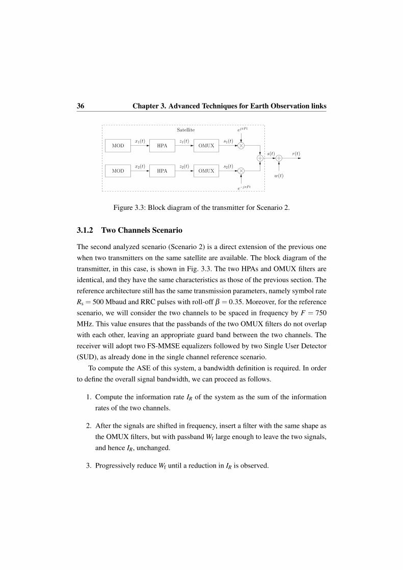
3.1.2 Two Channels Scenario
The second analyzed scenario (Scenario 2) is a direct extension of the previous onewhen two transmitters on the same satellite are available. The block diagram of thetransmitter, in this case, is shown in Fig. 3.3. The two HPAs and OMUX filters areidentical, and they have the same characteristics as those of the previous section. Thereference architecture still has the same transmission parameters, namely symbol rateRs = 500 Mbaud and RRC pulses with roll-off β = 0.35. Moreover, for the referencescenario, we will consider the two channels to be spaced in frequency by F = 750MHz. This value ensures that the passbands of the two OMUX filters do not overlapwith each other, leaving an appropriate guard band between the two channels. Thereceiver will adopt two FS-MMSE equalizers followed by two Single User Detector(SUD), as already done in the single channel reference scenario.
To compute the ASE of this system, a bandwidth definition is required. In orderto define the overall signal bandwidth, we can proceed as follows.
1. Compute the information rate IR of the system as the sum of the informationrates of the two channels.
2. After the signals are shifted in frequency, insert a filter with the same shape asthe OMUX filters, but with passband Wf large enough to leave the two signals,and hence IR, unchanged.
3. Progressively reduce Wf until a reduction in IR is observed.

3.2. Optimization of the Reference Architecture 37
4. Define the bandwidth of the system as the smallest value of Wf which causes areduction of IR not greater than 1% with respect to the case without the filter.
With this procedure, we defined the reference bandwidth as Wf = 1320 MHz, and wecan compute the ASE as
ASE =IR
TsWf[bit/s/Hz].
Again, the ASE will be computed as a function of Psat/N. However, in this casePsat is the overall available power of the HPA, and hence it is twice as much as thepower available in Scenario 1. Also in this case, N = N0Wf is the noise power in theconsidered bandwidth.
3.2 Optimization of the Reference Architecture
For the optimization of this reference system, we consider the application of advancedtechniques at both the transmitter and receiver sides. The analyzed solutions can besummarized as follows.
The optimization of the symbol rate and of the signal bandwidth. The symbol rateand the roll-off factor of pulse p(t) can be jointly optimized to find the best setting fora fixed bandwidth of the OMUX filter. Hence, we will consider the adoption of lowerroll-off values and an increased symbol rate. This kind of optimization is similar tothat performed in [23] for the extensions of the DVB-S2 system (DVB-S2X [1]).
The application of faster-than-Nyquist or time-frequency packing. In satellite sys-tems, orthogonal signaling is often adopted to avoid ISI at least in the absence of non-linear distortions. When finite-order constellations are considered, it is well knownthat the ASE can be improved by relaxing the orthogonality condition, thus inten-tionally introducing a certain amount of controlled ISI. In this case, the systems areworking in the domain of the Faster-than-Nyquist paradigm [40, 41, 42, 43] or its ex-tension known as time packing [44, 20, 45]. The effect of this technique is somehowsimilar to the increase of the signal bandwidth, as shown in [45]. In fact, for fixedtransmitter filter bandwidths, an increase of the signal bandwidth will result in an in-crease of ISI. However, the use of time packing adds another degree of freedom that
38 Chapter 3. Advanced Techniques for Earth Observation links
can be properly exploited. From an operational point of view, we can define the sym-bol interval as Ts = τT , where T is half of the main lobe duration of p(t) and τ ≤ 1 isthe time-packing factor, which will be properly selected to maximize the efficiencyof the system. The same concept has been extended to the frequency domain, whenmore channels are present. Hence, in Scenario 2, we can also apply the frequencypacking technique, by reducing the frequency spacing F and jointly increasing thesymbol rate, thus introducing controlled ICI.
The use of a more sophisticated receiver. The increased ISI (in both scenarios)and ICI (in Scenario 2) introduced by the two previously mentioned techniques canbe more effectively coped with by adopting more sophisticated receiver architectures.In particular, we will adopt the adaptive CS receiver proposed in [15], which con-sists of an FS equalizer, an adaptive CS filter and a BCJR detector [6]. This receiverstructure is based on the CS technique [12], which allows to design the information-theoretically optimal mismatched receiver for a given reduced complexity. When thechannel memory at the detector is set to L = 0, this scheme is equivalent to the FS-MMSE receiver of the reference scenario. Moreover, for Scenario 2, the adaptive CSfilters can be followed not only by a SUD, as in Scenario 1, but also by a MultiuserDetector (MUD), which is expected to better handle the ICI arising from the appli-cation of the frequency packing technique, at the price of an increased complexity ofthe detection stage [46]. For the SUD receiver of Scenario 2, we also implementeda receiver based on the IC-CS [13] and showed the attainable gains. Moreover, tofully exploit the available bandwidth, we propose an alternative transmitter structure,which consists in removing the two OMUX filters at the output of the transmitters,and introducing a single large filter with bandwidth Wf. In this bandwidth, we willallow the two signals to be as overlapped as possible, and we will adopt both theSUD and the MUD. The block diagram of the transmitter for this new architecture isshown in Fig. 3.4, where the BPF is a band-pass filter with bandwidth Wf. It shouldbe noted, however, that the combination of two Radio Frequency (RF) signals over-lapping in frequency can cause significant power losses. This issue will be brieflyaddressed later.
The use of the Alamouti space-time block code. For Scenario 2, we will also con-

3.2. Optimization of the Reference Architecture 39
e−jπF t
s1(t)
s2(t)
ejπF t
BPF
w(t)
x1(t)
x2(t)
s(t) r(t)
MOD HPA
MOD HPA
Satellite
Figure 3.4: Evolution of the transmitter for the Scenario 2.
sider the application of the Alamouti space-time block code [47] as a convenientalternative. Unlike what happens in [47], we do not use the Alamouti scheme toachieve a diversity gain, but as a way of orthogonalizing the two signals. In thisscheme, the two transmitters exchange the two information sequences in two suc-cessive transmission intervals. At the receiver, two consecutive observed sequencesare properly processed and then fed to two SUDs. In this way we can always trans-mit fully overlapped signals and perform only lower complexity operations at thereceiver. To preserve the orthogonality of the two signals, in this approach, the sameinformation has to be transmitted twice over two consecutive intervals. Moreover,the nonlinear effects introduced by the HPA prevent an ideal cancellation of the in-terfering signal, thus affecting the performance of the detector. More insights on theapplication of the Alamouti technique on a nonlinear satellite channel can be foundin [48], where it is also demonstrated that the Alamouti scheme is convenient whencompared to Time Division Multiplexing (TDM) or Frequency Division Multiplex-ing (FDM) schemes. On an ideal channel, the three schemes are perfectly equivalent;however, TDM requires that, in each transmission slot, each transmitter uses doublepower, which might not be a feasible solution in a peak-power limited channel suchas that under consideration. The performance of FDM, on the other hand, is signifi-cantly degraded by the interference of the adjacent channel, which derives from thespectral regrowth caused by the HPA [48].
The use of a more advanced predistortion algorithm. As mentioned, for the ref-erence scenario, we will adopt the static DPD of [26, 27]. This algorithm consists

40 Chapter 3. Advanced Techniques for Earth Observation links
HPA
g
z(t)v(t)x(t)Volterra
coeff.comp.
x(t)
SPD
v(t)
Figure 3.5: Block diagram of the proposed SPD.
of a training phase, in which the predistorted constellation is computed based on thechannel outputs. The information bits are then mapped on this constellation instead ofusing the real one. This approach is convenient in a scenario like the DVB-S2 model,where predistortion takes place at a transmitter on the ground, that is, remotely fromthe source of nonlinearity, and not directly before the HPA. In this scenario, instead,data are generated directly on the satellite, and they can be predistorted exactly be-fore the amplifier. This fact allows us to use a Signal PreDistorter (SPD) instead of aDPD. SPDs have been widely studied in the literature [35, 36, 37] due to their abilityto work on the samples of the continuous time signal rather than on the transmittedsymbols.
We will now introduce a new signal predistortion algorithm, whose performancewill be investigated in the next section. The block diagram of the proposed SPDis shown in Fig. 3.5, and it is composed of two main blocks. The block labeled as“Volterra” takes as input the signal (3.1) and outputs the signal
v(t) =S
∑s=0
gsx(t)|x(t)|2s , (3.2)
that is, a memoryless Volterra series of order 2S+ 1 taking into account odd orderterms only. The second block is a hard limiter, which clips the amplitude of the signal

3.3. Numerical Results 41
and whose input-output relationship can be expressed as
v(t) =
v(t) if |v(t)| ≤ 1
1 otherwise.
We have verified that the presence of this hard limiter significantly improves theperformance, as in this way the nonlinear part of the characteristic is completelyavoided. The complex coefficients g = {gs}S
s=0 in (3.2) are selected to minimize themean-square error between the transmitted hard-limited signal x(t) and the signal atthe output of the HPA, z(t):
g = argminCS+1
E[|z(t)− x(t)|2
]. (3.3)
During the training stage, the block “coefficients computation” in Fig. 3.5 performsthe minimization (3.3) through the algorithm described in [49] and included in thenonlinear optimization package [50]. We point out that this predistortion scheme canalso be used jointly with the described DPD (we will denote this as DSPD scheme):the predistortion of the constellation can be used to further contrast the residual dis-tortions that the SPD alone has not been able to invert.
3.3 Numerical Results
In this section, we show the results, in terms of ASE, of the proposed transceivertechniques, for the two scenarios under consideration. We adopt the M−ary PhaseShift Keying (PSK) and APSK constellations foreseen by the CCSDS standard [38],with cardinality ranging from 4 (QPSK) to 32. For 64APSK, we adopt a constellationintroduced by the DVB-S2X standard [1], which ensures slightly better performancewith respect to that of CCSDS. Unless otherwise stated, the ASE curves will be com-puted as the envelope of the ASEs of all modulation formats. This means that, foreach value of Psat/N, we will choose the modulation format achieving the best ASE.Moreover, for each case, the IBO of the HPA will be optimized to maximize the ASE.
42 Chapter 3. Advanced Techniques for Earth Observation links
3.3.1 Scenario 1
Fig. 3.6 shows the ASE of the system with an optimized symbol rate, in comparisonwith the reference scenario. The roll-off factor is set to β = 0.35 for all curves. Wealso compare the performance of the static DPD with the SPD and DSPD schemesproposed in the previous section, with S = 3 (that is, the signal is modeled as a 7thorder nonlinearity), for increasing values of the memory considered at the receiver,L = 0, 1. The details on the symbol rate for the curves of Fig. 3.6 are reported inTable 3.1 for DPD and SPD. The first thing we notice is that the SPD is clearly con-venient over the DPD, with the DSPD that grants some further limited gains in someparts of the curves. We also notice that, in the medium-low Psat/N range, increasingthe complexity of the detector can provide only very limited advantages. More rel-evant differences arise in the high Psat/N region, where the increased memory canbetter cope with the interference introduced by the high symbol rate values. In allcases, however, the gains over the reference scenario are significant. We also mentionthat we have performed the same analysis by using reduced roll-off values, namely0.2 and 0.1, but the results do not improve with respect to the reference value of 0.35.This is reasonable because, by optimizing the symbol rate, we are also selecting thebest signal bandwidth, and hence a further optimization of the roll-off is not required.Interestingly, the proposed SPD allows the system to work with a much lower IBOwith respect to the DPD. In fact, while the SPD requires an IBO of 3 dB only for64APSK, the DPD needs an IBO of 3 dB for 16APSK, 6 dB for 32APSK, and 9 dBfor 64APSK, to achieve the presented performance. A higher IBO also has a negativeimpact on the HPA efficiency, and, in turn, on the power dissipated on board.
We next consider the application of time packing. For this analysis, only the DPDhas been applied, but similar results can be obtained for the SPD. Fig. 3.7 shows theASE for QPSK and 8PSK when the value of τ has been optimized. The memoryof the BCJR has been set to L = 4, which, we found, is practically optimal for thisscenario. Both curves have been computed starting from the reference symbol rateRs = 500 Mbaud. We see that, although the symbol time is optimized, time packingcannot reach the same performance as transmission with orthogonal signaling withincreased symbol rate. In fact, Fig. 3.7 also reports the ASE of 8PSK and 16APSK

3.3. Numerical Results 43
0
1
2
3
4
5
6
7
8
-10 -5 0 5 10 15 20 25 30
ASE
[bit/s/Hz]
Psat/N [dB]
2
2.5
3
3.5
8 10 12 14Reference
DPD, L = 0SPD, L = 0
DSPD, L = 0DPD, L = 1SPD, L = 1
DSPD, L = 1
Figure 3.6: ASE for Scenario 1 and optimized symbol rate.
Table 3.1: Optimized symbol rate Rs (in Mbaud) for the curves in Fig. 3.6.
Psat/N [dB]DPD SPD
L = 0 L = 1 L = 0 L = 1M Rs M Rs M Rs M Rs
-10 8 500 8 500 4 550 4 550
-5 8 550 8 550 8 500 8 500
0 8 600 8 600 8 550 8 550
5 8 650 8 650 8 650 8 650
10 16 650 16 650 16 650 16 650
15 32 650 16 850 32 650 16 800
20 64 650 32 800 64 650 64 650
25 64 650 64 800 64 650 64 800
30 64 700 64 800 64 700 64 800

44 Chapter 3. Advanced Techniques for Earth Observation links
0
1
2
3
4
5
-10 -5 0 5 10 15 20 25
ASE
[bit/s/Hz]
Psat/N [dB]
QPSK, L = 4, opt. τ8PSK, L = 4, opt. τ
8PSK, L = 0, opt. Rs
16APSK, L = 0, opt. Rs
Figure 3.7: ASE for Scenario 1 and time packing.
with optimized symbol rates. The latter curves achieve higher values of ASE witha much lower complexity, relying only on a symbol-by-symbol detector, with L =
0. This result is somewhat expected, as it is in line with that obtained for a DVB-S2X scenario in [24], which shows that the potential of time packing on the satellitechannel is very limited. However, it is important to remember that a sort of alternativeto time packing is already achieved by increasing the symbol rate of the signal. In fact,both techniques introduce interference to the signal.
Then, we investigate more in detail the performance of the proposed SPD. Fig. 3.8reports the ASE for orders of the SPD increasing from 1 to 7, when the detector withmemory L = 0 is adopted (similar conclusions can be drawn when L = 1). We seethat a 3rd order Volterra series is already practically optimal. We also notice thatthe DSPD has significant advantages when the 1st order series is adopted, while thegains are much more limited in the other cases. This analysis proves that most ofthe nonlinear effects are inverted by the SPD. Finally, Fig. 3.9 shows the PSD forthe predistorted signal at the output of the OMUX filter. We see that the proposed

3.3. Numerical Results 45
0
1
2
3
4
5
6
7
8
-10 -5 0 5 10 15 20 25 30
ASE
[bit/s/H
z]
Psat/N [dB]
3.5
4
4.5
5
14 16 18 1st order SPD3rd order SPD5th order SPD7th order SPD
1st order DSPD3rd order DSPD5th order DSPD7th order DSPD
Figure 3.8: SPD and DSPD performance in Scenario 1.
SPD does not increase the side lobes of the spectrum with respect to the absenceof predistortion (no pred. PSD). The transmission parameters for Fig. 3.9 are theoptimal ones at Psat/N = 10 dB, but the same happens for other configurations andfor the DSPD scheme.
3.3.2 Scenario 2
Following from the results obtained for Scenario 1, in Scenario 2 we will not considerthe application of time packing as a possible solution, and we will fix the roll-offfactor of the shaping pulse to 0.35. Moreover, for the sake of clarity, we will notpresent results for the SPD. We have, however, verified that the performance of theSPD is practically equivalent to that of the DSPD scheme.
Fig. 3.10 compares the envelope of the ASE for different transceiver schemes,all considering a memory L = 0 at the detector. In particular, the curve labeled withOMUX only differs from the reference in the symbol rate and central frequency ofthe two channels, which have been selected to maximize the ASE. As we see, this
46 Chapter 3. Advanced Techniques for Earth Observation links
-100
-80
-60
-40
-20
0
-2000 -1500 -1000 -500 0 500 1000 1500 2000
PSD
[dB]
Frequency [MHz]
no pred.SPD 1st ord.SPD 3rd ord.SPD 5th ord.SPD 7th ord.
Figure 3.9: PSD of the transmitted signal with SPD in Scenario 1, 16APSK, IBO = 0dB, Rs = 650 Mbaud.
optimization alone allows significant gains. Further gains can be achieved by remov-ing the two OMUX filters and introducing the single filter with bandwidth Wf (noOMUX curves). In this case, we can use the MUD to fully exploit the ICI gener-ated by the frequency packing, achieving excellent performance at the price of anincreased complexity with respect to the SUD. Finally, the Alamouti scheme can out-perform the SUD with basically the same complexity, although it is still far fromthe MUD. To conclude the analysis, we can confirm the superiority of the proposed(D)SPD scheme over the DPD for all receiver architectures.
Next, we increase the memory considered at the detector. We point out that thisinvestigation has been carried out only for the schemes without the two inner OMUXfilters. This is because a higher complexity detector is needed to cope with the in-creased interference which arises when the filters are removed. The resulting ASEcurves are shown in Fig. 3.11. If we compare them with the corresponding curves inFig. 3.10, we see that both the SUD and the Alamouti schemes have only small ben-efits with respect to symbol-by-symbol detection, and only in the high Psat/N range.

3.3. Numerical Results 47
0
1
2
3
4
5
6
7
8
-10 -5 0 5 10 15 20 25
ASE
[bit/s/H
z]
Psat/N [dB]
ReferenceDPD, SUD, with OMUXDPD, SUD, no OMUXDPD, MUD, no OMUX
DPD, AlamoutiDSPD, SUD, no OMUXDSPD, MUD, no OMUX
DSPD, Alamouti
Figure 3.10: ASE for Scenario 2 with L = 0.
For complexity reasons, we have not simulated the performance of the MUD withL = 1. However, we see that the symbol-by-symbol MUD in Fig. 3.10 has better per-formance than the other two receiver schemes, even when part of the memory is takeninto account at the detector.
Let us now better characterize the behavior of the MUD in this scenario. Ta-ble 3.2 reports the optimized values of symbol rate Rs and frequency spacing F forthe scheme adopting the DSPD and the MUD with L = 0. We can notice that, asPsat/N increases, the symbol rate increases and the frequency spacing quickly fallsto 0, allowing the two signals to be completely overlapped in frequency. The samebehavior can be observed with the DPD instead of the DSPD. Fig. 3.12 shows howthe ASE varies as a function of Rs for increasing values of Psat/N, for the MUD re-ceiver. While the global maximum is that reported also in Table 3.2, it is interesting tonotice that another lower peak arises in correspondence with a lower symbol rate. Ifwe compare this second peak with the curves in Fig. 3.10, we see that it exactly cor-responds to the ASE achieved by the SUD receiver. Moreover, we have verified that

48 Chapter 3. Advanced Techniques for Earth Observation links
0
1
2
3
4
5
6
7
8
-10 -5 0 5 10 15 20 25
ASE
[bit/s/H
z]
Psat/N [dB]
ReferenceDPD, SUD, no OMUX
DPD, AlamoutiDSPD, SUD, no OMUX
DSPD, Alamouti
Figure 3.11: ASE for Scenario 2 with L = 1.
Table 3.2: Details of the ASE in Fig. 3.10 for the DSPD and the MUD receiver.Psat/N [dB] M Rs [Mbaud] F [MHz]
-10 4 572 594
-5 8 660 594
0 8 1364 66
5 8 1408 0
10 8 1408 0
15 16 1452 0
20 32 1452 0
25 64 1452 0

3.3. Numerical Results 49
1
2
3
4
5
6
7
8
9
400 600 800 1000 1200 1400 1600 1800
ASE
[bit/s/Hz]
Rs [Mbaud]
Psat/N = 0 dBPsat/N = 5 dB
Psat/N = 10 dBPsat/N = 15 dB
Psat/N = 20 dBPsat/N = 25 dB
Figure 3.12: ASE as a function of Rs for the MUD receiver.
also the values of Rs and F associated with the second peak are almost the same asthe optimized values for the SUD. We can conclude that the second peak correspondsto a combination of symbol rate and frequency spacing in which the impact of ICI isalmost negligible, and hence the SUD and the MUD have the same performance. Thisfact can be verified in Fig. 3.13, which reports the ASE and the optimal frequencyspacing F for each value of Rs, for Psat/N = 25 dB. The value of F corresponding tothe second peak is large enough to practically avoid any overlap of the two signals.The same behavior is observed for other values of Psat/N.
It has been proved in [48] that, in a peak-power limited scenario with multipletransmitters and a MUD at the receiver, it is convenient to adopt PSK constellationsrather than APSKs. Moreover, it has been shown in [51] that a phase shift of π/M be-tween the two constellations ensures a simple design and good performance. Fig. 3.14reports the ASE as a function of Rs with these phase-shifted PSK constellations. Thepeak of the ASE is almost the same as that achieved in Fig. 3.12 with APSKs. How-ever, the second peak is much lower, to indicate that this configuration is not suitable

50 Chapter 3. Advanced Techniques for Earth Observation links
4
4.5
5
5.5
6
6.5
7
7.5
8
400 600 800 1000 1200 1400 1600 18000
125
250
375
500
625
750
875
1000
ASE
[bit/s/H
z]
F[M
Hz]
Rs [Mbaud]
ASEF
Figure 3.13: ASE and F as a function of Rs for the MUD receiver and Psat/N = 25dB.
for single-user detection.
It is interesting to see also the improvement that can be achieved through the useof the CS receiver extension proposed in [13] and [14]. As explained in Chapter 1,it allows an interference cancellation based on soft-symbol feedback. After a firstiteration between the detector and the decoder, the soft-symbols are computed, thefilters and the trellis are updated according to the quality of the soft-symbol feedback,and then the soft-symbols are filtered and removed from the received signal samples.This procedure is thus iterated since at each iteration between detector and decoderthe quality of the feedbacks should improve. The problem is that it is not possible tocompute the AIR of this receiver. In fact, the receiver is changing at each iteration.The only way to test its performance is by using practical codes, testing its PER.To have a fair comparison, we computed also the PER using a simple CS detectorthat performs an iterative detection and decoding, without interference cancellation(i.e., the filter and trellis remain the same at each iteration). We employed in boththe cases the DVB-S2X LDPC codes, with a maximum of 50 iteration at the decoder

3.3. Numerical Results 51
1
2
3
4
5
6
7
8
9
400 600 800 1000 1200 1400 1600 1800
ASE
[bit/s/Hz]
Rs [Mbaud]
Psat/N = 0 dBPsat/N = 5 dB
Psat/N = 10 dBPsat/N = 15 dB
Psat/N = 20 dBPsat/N = 25 dB
Figure 3.14: ASE as a function of Rs for the MUD receiver and PSK constellations.
and 5 iterations between detector and decoder. We show for reference also the Psat/Nvalue at which the receiver should reach the coding-modulator efficiency rc log2 Mwith the non-iterative CS. Fig. 3.15 and Fig. 3.15 show the attainable results withan 8-PSK and a 16-APSK, employing Rs = 800 MHz. The fact that IC-CS receiverwith L = 0 outperforms the information rate limit is not surprising, since that is avalid upper bound only for the CS without IC. With an 8-PSK, the detector withL = 0 and IC has almost the same performance of a detector with L = 1 and noIC, while for the 16-APSK the loss is wider. However, the gap between the detectorwith and without IC for L = 0 is remarkable (∼ 3 dB and ∼ 10 dB for the 8-PSKand 16-APSK, respectively). It has to be noticed that for L = 0 the IC-CS becomesan MMSE receiver with interference cancellation [52, 53, 54]. However, a memoryL≥ 0 is not useful in this case for an IC receiver: the channel memory introduced bythe bandwidth optimization is almost completely captured by a detector with L = 1without performing IC. So, there would be no interference to be cancelled with L = 1for an IC-CS detector, and the receiver would become only more complex, without

52 Chapter 3. Advanced Techniques for Earth Observation links
10−4
10−3
10−2
10−1
100
5 6 7 8 9 10 11 12
= 0Ir = 1
PER
Psat/N [dB]= 0 = 1 IC, = 0
LL
L L L
,
Figure 3.15: PER performance comparison between the simple CS and IC-CS detec-tor, using an 8−PSK with rc = 23/36 at Rs = 800MHz.
any gain in SNR.
We also want to add a comment on some of the theoretical results in this section.For Scenario 2, our results assumed that an ideal combination of the two signals in RFafter the HPA is possible. However, the combining of RF of two signals overlappingin frequency will incur a significant loss in the order of 3 dB. Hence, to take intoaccount this effect, the optimized curves of Figs. 3.10 and 3.11 have to be shiftedby 3 dB to the right. We can clearly see how in this case the possible gains over thereference architecture are much more limited. A more effective way to exploit the twoavailable HPAs is to combine them to form an equivalent HPA with double power.This solution reduces to a single-carrier scenario with double power, and hence it isa direct extension of Scenario 1. The corresponding ASE can be simply achieved byshifting the curves in Fig. 3.6 by 3 dB to the left.

3.4. Conclusions 53
10−4
10−3
10−2
10−1
100
10 12 14 16 18 20 22 24 26
= 0Ir, = 1
PER
Psat/N [dB]L = 0 L = 1 IC, L = 0
L L
Figure 3.16: PER performance comparison between the simple CS and IC-CS detec-tor, using an 16−APSK with rc = 3/4 at Rs = 800MHz.
3.4 Conclusions
We have analyzed two different high rate telemetry scenarios, with one and two chan-nels, respectively. We have shown that, in both cases, significant spectral efficiencygains are possible with respect to the current configuration through the application ofadvanced techniques at the transmitter and at the receiver. In particular, we have pro-posed a new signal predistortion algorithm, which exhibits very good performance inthe considered scenarios. We have also shown how the proposed signal predistortercan be combined with classical data predistortion techniques, to further enhance theperformance. We have then optimized the symbol rate and introduced more sophis-ticated detection algorithms. For the single-carrier scenario, the proposed solutionsallow gains of about 3 dB over the reference architecture at a spectral efficiency of4 bit/s/Hz. For the scenario with two channels, we have also demonstrated that theapplication of frequency packing, coupled with the proposed signal predistorter atthe transmitter and a multiuser detector at the receiver, can achieve excellent results
54 Chapter 3. Advanced Techniques for Earth Observation links
when compared with all other techniques, at the price of an increased complexity ofthe detection stage. We have also proposed the use of the Alamouti space-time blockcode as a lower complexity alternative. For this scenario, the gains with respect tothe reference architecture vary from 4 to 7 dB at a spectral efficiency of 4 bit/s/Hz,depending on the adopted transceiver scheme. Furthermore, we showed that on thetwo channels scenario with an optimized symbol-rate value, the IC-CS at L = 0 has asignificant gain compared to a CS receiver with the same memory (∼ 3 dB for 8-PSKand ∼ 10 dB for 16-APSK). For an 8-PSK constellation, the IC-CS at L = 0 reachesalmost the same performance of a CS receiver with L = 1 while the 16-APSK showsa larger loss of ∼ 4 dB.

Chapter 4
LEO Satellite Receiver for LoRaModulated Signals
The IoT devices are becoming widespread and used for many different purposes.They make use of different transmission schemes and protocols and need gatewaysto connect to the Internet. However, it is hard to have a complete coverage for thecommunication from the IoT device to the gateway (uplink), especially in rural ar-eas. A swarm of LEO satellites could thus help in these scenarios, by relaying themessages intended for the gateway when the devices are located in areas far from thecities. We base the study on one of the most promising Low Power-Wide Area Net-work (LPWAN) solution: LoRa. These devices work with a proprietary modulationformat at physical layer [2]. Higher layers are defined in the LoRaWAN specificationsby the LoRa Alliance [55].
In this chapter, we analyze the LoRa modulation and its receiver scheme. Then,we propose an improved receiver to cope with typical LEO satellite communicationsimpairments (i.e., Doppler shift and Doppler rate).
This is the foundation for the realization of a complete system simulator thatincludes the interference coming from all the users in the field of view of the satellite.The description of this simulator and the results of the study can be found in [3].

56 Chapter 4. LEO Satellite Receiver for LoRa Modulated Signals
4.1 Lora signal and its properties
The complex envelope of a LoRa signal can be expressed as
s(t) =
√2Es
Texp
{j2πB
∫ t
−∞
[∑k
Γ(τ− kT ;ak)
]dτ
}(4.1)
where Es is the energy per information symbol, T the symbol interval, B a proper pa-rameter (B = 125, 250, or 500 kHz in the LoRaWAN standard), {ak} the transmittedsymbols belonging to the alphabet {0,1, . . . ,N−1}, being the cardinality N a powerof 2 and,
Γ(τ;ak) = mod(
τ−akT/NT
)rect
( tT
). (4.2)
In (4.2), the mod(·) function is the modulo operation in [−0.5,0.5). We will defineSF = log2 N (7 ≤ SF ≤ 12 in the LoRaWAN standard). Parameters B, N, and T arerelated through the equation
BT = N = 2SF . (4.3)
This means that, for a given bandwidth B, the higher the alphabet’s cardinality N,the higher the symbol duration T . Fig. 4.1 reports all possible functions Γ(t;ak) fordifferent values of ak in the case of SF = 2 (N = 4). This parameter choice is notforeseen by the standard but is useful to easily understand the modulation format.
This modulation format is characterized by the following important properties:
1. it has a constant envelope (and thus it is insensitive to nonlinear distortions);
2. it has a continuous phase (and thus its spectrum is compact);
3. it has no memory;
4. the occupied bandwidth is B (with good approximation).
Properties 1 and 2 are obvious from the complex envelope expression (4.1). Property3 easily follows from the definition of Γ(t;ak) in (4.2). In fact, the integral of Γ(t;ak)
is zero, no matter the value of ak. Thus, if we consider the interval [kT −T/2,kT +
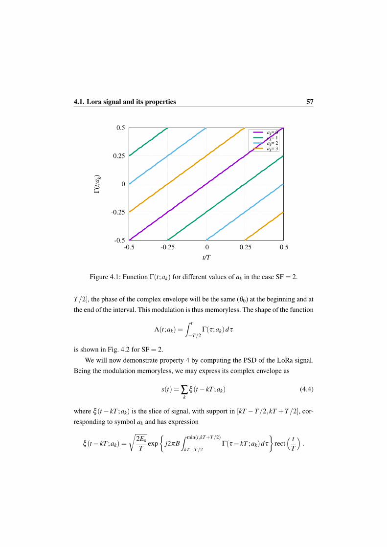
4.1. Lora signal and its properties 57
-0.5
-0.25
0
0.25
0.5
-0.5 -0.25 0 0.25 0.5
Γ(t
;ak)
t/T
akak= 1ak= 2ak= 3
= 0
Figure 4.1: Function Γ(t;ak) for different values of ak in the case SF = 2.
T/2], the phase of the complex envelope will be the same (θ0) at the beginning and atthe end of the interval. This modulation is thus memoryless. The shape of the function
Λ(t;ak) =∫ t
−T/2Γ(τ;ak)dτ
is shown in Fig. 4.2 for SF = 2.
We will now demonstrate property 4 by computing the PSD of the LoRa signal.Being the modulation memoryless, we may express its complex envelope as
s(t) = ∑k
ξ (t− kT ;ak) (4.4)
where ξ (t− kT ;ak) is the slice of signal, with support in [kT −T/2,kT +T/2], cor-responding to symbol ak and has expression
ξ (t− kT ;ak) =
√2Es
Texp{
j2πB∫ min(t,kT+T/2)
kT−T/2Γ(τ− kT ;ak)dτ
}rect
( tT
).
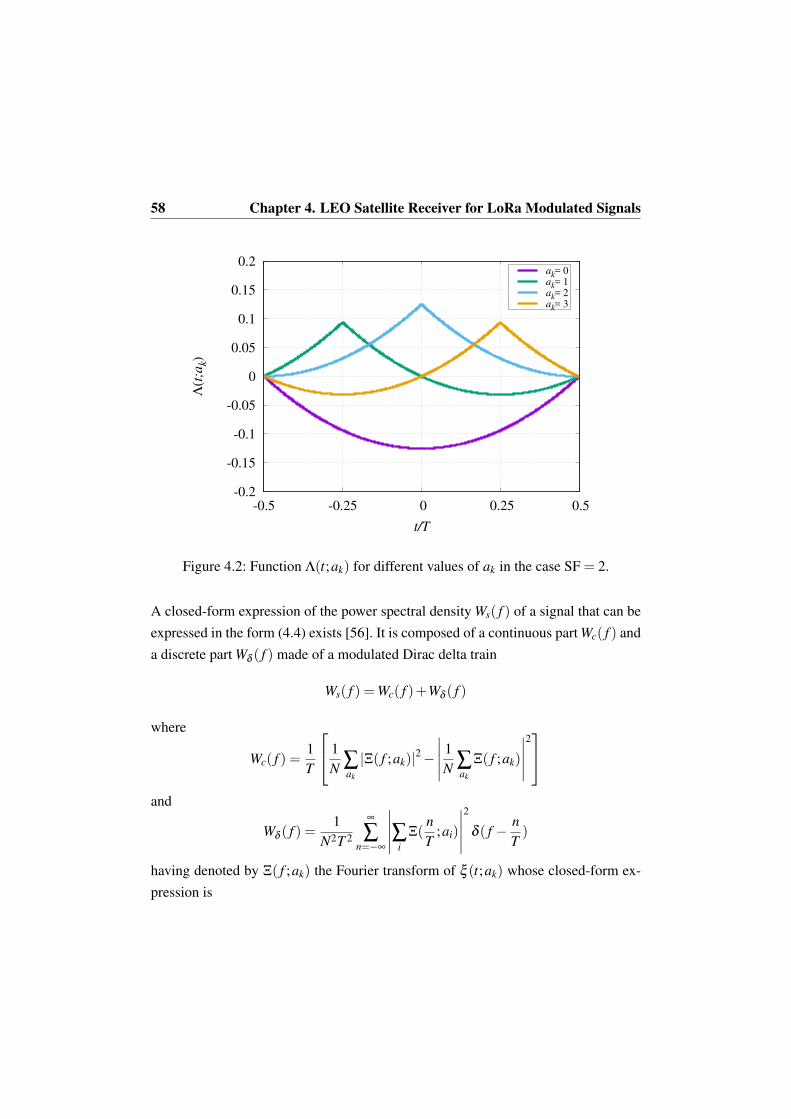
58 Chapter 4. LEO Satellite Receiver for LoRa Modulated Signals
-0.2
-0.15
-0.1
-0.05
0
0.05
0.1
0.15
0.2
-0.5 -0.25 0 0.25 0.5
Λ(t
;ak)
t/T
ak= 0ak= 1ak= 2ak= 3
Figure 4.2: Function Λ(t;ak) for different values of ak in the case SF = 2.
A closed-form expression of the power spectral density Ws( f ) of a signal that can beexpressed in the form (4.4) exists [56]. It is composed of a continuous part Wc( f ) anda discrete part Wδ ( f ) made of a modulated Dirac delta train
Ws( f ) =Wc( f )+Wδ ( f )
where
Wc( f ) =1T
1
N ∑ak
|Ξ( f ;ak)|2−∣∣∣∣∣
1N ∑
ak
Ξ( f ;ak)
∣∣∣∣∣
2
and
Wδ ( f ) =1
N2T 2
∞
∑n=−∞
∣∣∣∣∣∑iΞ(
nT
;ai)
∣∣∣∣∣
2
δ ( f − nT)
having denoted by Ξ( f ;ak) the Fourier transform of ξ (t;ak) whose closed-form ex-pression is
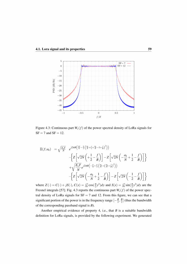
4.1. Lora signal and its properties 59
−45
−40
−35
−30
−25
−20
−15
−10
−5
0
5
−1 −0.5 0 0.5 1
PSD
[dB/H
z]
f/B
SF= 7SF= 12
Figure 4.3: Continuous part Wc( f ) of the power spectral density of LoRa signals forSF = 7 and SF = 12.
Ξ( f ;ak) =√
EsTN e j2πB
(3T8 − T
2
(akN +(+ ak
N −1+ fB)
2))
·{
Z[√
2N(+
12− f
B
)]−Z
[√2N(−ak
N+
12− f
B
)]}
+
√EsTN
e j2πB(− T
8 +T2
(akN +( ak
N + fB)
2))
·{
Z[√
2N(−ak
N+
12− f
B
)]−Z
[√2N(−1
2− f
B
)]}
where Z (·) = C(·)+ jS(·), C(x) =∫ x
0 cos(π
2 y2)dy and S(x) =∫ x
0 sin(π
2 y2)dy are theFresnel integrals [57]. Fig. 4.3 reports the continuous part Wc( f ) of the power spec-tral density of LoRa signals for SF = 7 and 12. From this figure, we can see that asignificant portion of the power is in the frequency range [−B
2 ,B2 ] (thus the bandwidth
of the corresponding passband signal is B).Another empirical evidence of property 4, i.e., that B is a suitable bandwidth
definition for LoRa signals, is provided by the following experiment. We generated

60 Chapter 4. LEO Satellite Receiver for LoRa Modulated Signals
signal s(t) according to (4.1) and then sampled it with Ns samples per symbol time.The sampling frequency is thus Fs =
NsT . Samples {s(kT/Ns)} are then interpolated
by using the Whittaker–Shannon interpolation formula [58], thus obtaining the in-terpolated signal s(t). In Figs. 4.4 we report, for the cases SF = 7 and SF = 12, thenormalized MSE
ε2 =
12Es
E{∫ T/2
−T/2|s(t)− s(t)|2 dt
}
where E{·} denotes expectation, as a function of Ns/N. It can be observed that theerror is negligible when Ns ≥ N. Thus, a sampling frequency Fs ≥ N
T is sufficient toensure the reconstruction of the original signal from its samples with a very goodapproximation. By using (4.3), we obtain that the sampling frequency must be suchthat
Fs ≥NT
= B . (4.5)
According to the sampling theorem, we know that signal s(t) can be reconstructedfrom its samples taken at a frequency Fs which is twice its bandwidth. Hence, from(4.5) we infer that a good estimate of the bandwidth of s(t) is B/2, and thus B is agood estimate of the bandwidth of the corresponding passband signal.
From the observation of Fig. 4.1, we can easily understand that we may express
Γ(t;ak) = Γ(t;0)+Φ(t;ak)
i.e., as a first contribution which is the value of Γ(t;ak) corresponding to symbolak = 0, thus common to all terms, plus a second term which depends on ak and canbe expressed as
Φ(t;ak) =
−ak
N +1 for − T2 ≤ t ≤−T
2 + akTN
−akN for − T
2 + akTN < t ≤ T
2
. (4.6)
Φ(t;ak) is thus a piecewise constant and is shown in Fig. 4.5 for different values of ak
in the case of SF = 2. Hence, the complex envelope of a LoRa signal in the genericinterval [kT −T/2,kT +T/2] (and thus the slice of signal we called ξ (t− kT ;ak))can be equivalently expressed as
ξ (t− kT ;ak) = ξ (t− kT ;0)exp{
j2πB∫ t
kT−T/2Φ(τ− kT ;ak)dτ
}

4.1. Lora signal and its properties 61
0
0.2
0.4
0.6
0.8
1
1.2
0 0.5 1 1.5 2
MS
E
Ns/N
SF=7
SF=12
Figure 4.4: Normalized mean square error between signals s(t) and s(t) versus Ns forSF = 7 and 12.
-1
-0.5
0
0.5
1
-0.5 -0.25 0 0.25 0.5
Φ(t
;ak)
t/T
ak= 0ak= 1ak= 2ak= 3
Figure 4.5: Function Φ(t;ak) for different values of ak in the case SF = 2.

62 Chapter 4. LEO Satellite Receiver for LoRa Modulated Signals
0
0.5
1
1.5
2
-0.5 -0.25 0 0.25 0.5
Ψ(t
;ak)/
π
t/T
ak= 0ak= 1ak= 2ak= 3
Figure 4.6: Function Ψ(t;ak) for different values of ak in the case SF = 2.
where
ξ (t− kT ;0) =
√2Es
Texp{
j2πB∫ t
kT−T/2Γ(τ− kT ;0)dτ
}(4.7)
is the slice of signal corresponding to ak = 0 and is a term whose phase quadraticallydepends on t (see Fig. 4.2). This is thus an up-chirp signal. We can define
Ψ(t− kT ;ak) = 2πB∫ t
kT−T/2Φ(τ− kT ;ak)dτ
obtainingξ (t− kT ;ak) = ξ (t− kT ;0)exp{ jΨ(t− kT ;ak)} .
The shape of Ψ(t;ak) is shown in Fig. 4.6 for SF = 2.Let us consider again the generic interval [kT −T/2,kT +T/2]. The slices ξ (t−
kT ;ak) corresponding to different symbols ak are not orthogonal. This can be simplyverified by computing the N×N matrix A whose elements are defined as
Ai,` =T
2Es
∫ kT+T/2
kT−T/2ξ (t− kT ;ak = i)ξ ∗(t− kT ;ak = `)dt .

4.1. Lora signal and its properties 63
Table 4.1: Normalized distance 1N ‖A− I‖F for different values of SF.
SF 1N ‖A− I‖F
2 2.1 ·10−1
3 1.3 ·10−1
4 7.8 ·10−2
5 4.6 ·10−2
6 2.7 ·10−2
7 1.6 ·10−2
8 9.4 ·10−3
9 5.5 ·10−3
10 3.2 ·10−3
11 1.9 ·10−3
12 1.1 ·10−3
Each value Ai,` represents the correlation between the signal corresponding to thesymbol ak = i and that corresponding to the symbol ak = `. If the slices ξ (t−kT ;ak)
were orthogonal, A would be the identity matrix. So, in order to understand how far isthis matrix from the identity one, we computed the normalized distance 1
N ‖A− I‖Fwhere I is the N×N identity matrix and ‖·‖F is the Frobenius norm. The values arereported in Table 4.1 for different values of SF. We may thus conclude that the slicesξ (t− kT ;ak) are not strictly orthogonal but can be approximated as such.
We said that signal s(t) has (approximately) a bandwidth B/2. It can be thusreconstructed from its samples when using a sampling frequency Fs = B = N/T .Without loss of generality, we can consider the interval [−T/2,T/2] and thus thetransmission of symbol a0. By sampling the signal t = `T/N, the N samples of thecomplex envelope are
ξ
(`TN
;a0
)= ξ
(`TN
;a0 = 0)
exp{
jΨ(`TN
;a0
)}, `=−N
2,−N
2+1, . . .0, . . . ,
N2−1.

64 Chapter 4. LEO Satellite Receiver for LoRa Modulated Signals
By unwrapping the phase Ψ(`TN ;a0
), it can be easily verified that
exp{
jΨ(`TN
;a0
)}= exp
{− j
2π
Na0
(`+
N2
)}, `=−N
2,−N
2+1, . . .0, . . . ,
N2−1.
and thus
ξ
(`TN
;a0
)= ξ
(`TN
;a0 = 0)
exp{− j
2π
Na0
(`+
N2
)}, `=−N
2,−N
2+1, . . .0, . . . ,
N2−1
or, equivalently,
ξn(a0) = ξn(a0 = 0)exp{− j
2π
Na0n}, n = 0,1, . . . ,N−1 (4.8)
having defined n = `+ N2 and
ξn(a0) = ξ
(n− N
2 TN
;a0
).
In other words, we can write the samples as the product of an up-chirp signal, com-mon to all signals, and a term whose phase is linearly decreasing with a slope depend-ing on the transmitted symbol. These discrete-time samples are, this time, orthogonal.In fact
N−1
∑n=0
ξn(a0 = i)ξ ∗n (a0 = `) =
N i = `
0 i 6= `.
This property will be used later. It is important to notice that if we sample with alower or higher sample frequency, this property no more holds, i.e., we can still writethe samples as the product of an up-chirp signal, common to all signals, and a secondterm depending on the transmitted symbol, but this time the phase of this second termis no more linearly decreasing.

4.2. Receiver design 65
4.2 Receiver design
4.2.1 Detection over an AWGN channel
Let us assume that an uncoded LoRa signal is transmitted over an AWGN channeland that ideal synchronization has been performed (synchronization issues will bediscussed in Section 4.2.3). Without loss of generality, since the modulation is memo-ryless, as discussed in the previous section, we can consider the interval [−T/2,T/2]focusing on detection of symbol a0 only. The complex envelope of the received signalcan thus be expressed as
r(t) = ξ (t;a0)+w(t)
where w(t) is the complex envelope of the additive white Gaussian noise. w(t) is acomplex Gaussian noise process with independent real and imaginary componentshaving zero mean and power spectral density N0.
From a conceptual point of view, optimal detection of LoRa signals can be per-formed through the following MAP detection strategy [59]1
a0 = argmaxa0
ℜ{z(a0)} (4.9)
having defined
z(a0) =∫ T/2
−T/2r(t)ξ ∗(t;a0)dt
i.e., z(a0) is obtained by sampling the received signal r(t) filtered through a filtermatched to ξ (t;a0). We can thus conclude that a sufficient statistic can be obtainedthrough a bank of N = 2SF filters matched to all possible waveforms waveformsξ (t;a0).
Although this receiver is quite simple from a conceptual point of view, it canhardly be implemented when N grows. Let us consider a digital implementation ofthe bank of N matched filters. In practical receivers, an approximated set of suffi-cient statistics is obtained through the technique described in [25]. It is assumed that
1This detection strategy has been obtained by exploiting the fact that ξ (t;a0) has a constant enve-lope.

66 Chapter 4. LEO Satellite Receiver for LoRa Modulated Signals
the LoRa low-pass equivalent is band-limited with bandwidth B/2—although this isnot strictly true as discussed in the previous section. The approximated statistics canbe obtained by sampling the received signal prefiltered by means of an ideal analoglowpass filter having bandwidth B/2. The use of an ideal filter ensures that the noisesamples are i.i.d. complex Gaussian random variables with independent components.As discussed in the previous section, we need at least N samples to represent thetransmitted signal in the interval [−T/2,T/2]. The complexity related to the imple-mentation of N matched filters is thus proportional to N2.
A significant complexity reduction can be obtained by exploiting (4.8). In fact,we can express the received samples as
rn = ξn(a0 = 0)e− j 2π
N a0n +wn
where wn are additive white Gaussian noise samples [25]. We can thus remove theup-chirp signal by computing
yn = r∗nξn(a0 = 0) = e j 2π
N a0n +w′n
where w′n are still additive white Gaussian noise samples since the up-chirp signalhas a constant amplitude and does not modify the noise statistics. The optimal MAPdetection strategy based on these samples can be expressed as
a0 = argmaxa0
ℜ
{N−1
∑n=0
yne− j 2π
N a0n
}. (4.10)
Looking at (4.10), we can recognize that the strategy can be expressed as
a0 = argmaxk
ℜ{Yk}
having defined
Yk =N−1
∑n=0
yne− j 2π
N kn
as the Discrete Fourier Transform (DFT) of samples yn. It can be thus efficientlycomputed through the Fast Fourier Transform (FFT) with complexity N log2 N = N ·SF.

4.2. Receiver design 67
10−9
10−8
10−7
10−6
10−5
10−4
10−3
10−2
10−1
100
8 9 10 11 12 13 14 15 16 17
SE
R
Es/N0 [dB]
SF=12 FFTSF=12 Matched filters
SF=12 TheoreticalSF=7 IFFT
SF=7 Matched filtersSF=7 Theoretical
Figure 4.7: SER for strategies (4.9) and (4.10).
The error probability of strategy (4.10) is known in an analytical form. In fact,since the discrete-time waveforms are orthogonal, the symbol error probability isexactly the same of any other orthogonal modulation scheme and reads [59]
PS = 1− 1√2π
∫ +∞
−∞
exp{−x2
2
}[1−Q
(x+
√2
Es
N0
)]N−1
dx (4.11)
where Q(·) is the Gaussian Q function.
As said, strategies (4.9) and (4.10) are only approximately equivalent. In fact,strategy (4.10) has been obtained under the approximated assumption that LoRa sig-nal (4.1) has a limited bandwidth B/2. Since this is not strictly true, it is interestingto evaluate the performance loss related to this approximation. In Fig. 4.7 we re-port the Symbol Error Rate (SER) versus Es/N0 of both strategies in the case of anuncoded transmission. For strategy (4.10) we also report the theoretical curve (4.11).The cases of SF= 7 and 12 have been considered. It may be observed that both strate-gies have practically the same performance. We can conclude that the approximationthat allows to obtain strategy (4.10) is very good.

68 Chapter 4. LEO Satellite Receiver for LoRa Modulated Signals
4.2.2 Noncoherent detection
Detection strategies (4.9) and (4.10) have been obtained under the assumption of idealsynchronization. We will now consider phase noise and the related performance lossit produces on strategies (4.9) and (4.10).
The optimal detection strategy in the presence of phase noise will depend on thechannel coherence time. When the channel coherence time is long enough, we canexploit its correlation to design a receiver with memory with a negligible performanceloss with respect to the case of ideal synchronization [60]. On the other end, when thechannel phase is assumed to change independently every symbol interval, the systemis again memoryless and the receiver will have the lowest possible complexity. It canbe easily shown that when the channel phase is assumed uniformly distributed and tochange independently every symbol interval, the strategies (4.9) and (4.10) become
a0 = argmaxa0|z(a0)| (4.12)
and
a0 = argmaxa0
∣∣∣∣∣N−1
∑n=0
yne− j 2π
N a0n
∣∣∣∣∣ . (4.13)
These kinds of strategies are called “noncoherent” in the literature. In particular, wewill consider strategy (4.13) only, since it can be implemented through the FFT. Fig.4.8 reports, for SF = 7 and 12, the SER performance of strategy (4.10) under theassumption of perfect knowledge of the channel phase (curves labeled “coherent”)and that of strategy (4.13) under the assumption that the channel phase is unknown,constant over a symbol interval, and changing independently every symbol interval.It can be observed that the performance loss of this noncoherent strategy is lower than0.5 dB. Thus, we believe that it is not worth investigating the possibility to exploitthe phase noise correlation in case of a longer coherence time.
4.2.3 Properties of LoRa signals to be exploited for synchronization
In this section, we will discuss on synchronization of LoRa signals. In particular,we will see which properties of LoRa signals can be exploited to perform frame,

4.2. Receiver design 69
10−6
10−5
10−4
10−3
10−2
10−1
100
8 9 10 11 12 13 14 15 16 17
SER
Es/N0 [dB]
SF=12 non-coherentSF=12 coherent
SF=7 non-coherentSF=7 coherent
Figure 4.8: SER comparison between strategies (4.10) and (4.13).
frequency, and timing synchronization. In Section 4.2.6, we will describe the entiresynchronization procedure.
The preamble of a LoRa packet is characterized by 8 consecutive up-chirps, two“special” modulated symbols, and 2.25 down-chirps. For the sake of clarity, we re-ported in Fig. 4.9 the value of the instantaneous frequency Γ(t) of these 12.25 pream-ble symbols. Let us consider an up-chirp signal in the reference interval [−T/2,T/2].It can be expressed in closed form as (see (4.7))
ξ (t;0) =
√2Es
Texp{
j2πB∫ t
kT−T/2Γ(τ;0)dτ
}
=
√2Es
Texp{
j2πB(
t2
2T− T
8
)}.
Let us now assume that a train of up-chirp signals experiences a delay τ (wewill assume 0 ≤ τ ≤ T ) and is affected by a frequency uncertainty ν (due to theuncertainty on the nominal frequency of the transmitted signal and the Doppler shift)

70 Chapter 4. LEO Satellite Receiver for LoRa Modulated Signals
0 2 4 6 8 10 12 14-1
-0.8
-0.6
-0.4
-0.2
0
0.2
0.4
0.6
0.8
1preambleSYNC WORDdownchirps
Figure 4.9: Instantaneous frequency Γ(t) for the sequence of preamble symbols inLoRaWAN.
and a phase shift θ0, in addition to the AWGN.2 The complex envelope of the receivedsignal can be thus expressed as
r(t) = β ∑k
ξ (t− kT − τ;0)e j(2πνt+θ0)+w(t)
where β is the attenuation due to propagation and w(t) is a complex Gaussian AWGNprocess.
Due to the presence of the frequency uncertainty ν , a discrete-time sufficientstatistic can still be obtained with the same technique already described in Section4.2.1, but N samples per symbol are no more sufficient. We will thus need to extractNo samples, with No > N, after the analog prefilter. These samples rn are then multi-plied by the complex conjugate of the samples of the original train of up-chirp signals(dechirping operation). This multiplication does not change the noise statistics. Thereceived samples after dechirping in the reference symbol interval [−T/2,T/2] canbe expressed as
yn = sn +wn , n =−No
2,−No
2+1, . . . ,
No
2−1 (4.14)
2We will consider the effect of the Doppler rate α later.

4.2. Receiver design 71
where wn is a discrete-time complex white Gaussian noise process and samples sn
can be expressed as
sn =
γe jθ1 exp{
j2π(B+ν−B τ
T
)n T
No
}−No
2 ≤ n <−No2 +N1
γe jθ2 exp{
j2π(ν−B τ
T
)n T
No
}−No
2 +N1 ≤ n < No2
where γ is a proper amplitude, taking into account the amplitude of the transmit-ted signal, the channel attenuation and the amplitude of the up-chirp signal used fordechirping, and having defined N1 =
⌊No
τ
T
⌋, where bxc denotes the largest integer
lower than or equal to x, and
θ1 = 2πB(
T2+
τ2
2T− τ
)+θ0
θ2 = 2πBτ2
2T+θ0 .
The computation of the Fourier transform of sequence sn, n=−No2 ,−No
2 +1, . . . , No2 −
1, will exhibit a maximum of amplitude max(N1,No−N1) either at frequency(ν−B τ
T
)
or at frequency(B+ν−B τ
T
). This maximum can be identified by using the Rife &
Boorstyn algorithm [61] which is based on two steps. A coarse search is first per-formed by computing some samples of the Fourier transform through the FFT andlooking for the maximum sample. An interpolation is then performed around thismaximum samples to refine the search (fine search step).
If we repeat the same operations for the down-chirp signal (this time using thedown-chirp signal to perform dechirping) we obtain again a maximum of ampli-tude max(N1,No−N1) but this time either at frequency
(ν +B τ
T
)or at frequency(
B+ν +B τ
T
). In the next section we will see how to exploit this property to perform
frame, frequency, and timing estimate.
When a Doppler rate α is also present, we observe an uncompensated frequencyoffset ν that varies linearly with time at a slope α . However, considering the valuesof α at stake, we can approximate this linear variation with a staircase, i.e., constantover a symbol and changing from symbol to symbol. So the frequency correspondingto the maximum amplitude of the Fourier transform, when performed on consecutive

72 Chapter 4. LEO Satellite Receiver for LoRa Modulated Signals
symbols, will increase or decrease linearly (depending on the sign of α). We have totake this into account when performing synchronization and detection.
4.2.4 Estimation of the frequency peaks
The estimation of the above-mentioned frequency peaks is a challenging task. In fact,the energy of a single sample is far lower than the noise power, leading to a high num-ber of outliers in the estimation process that could degrade the performance. Becauseof this, algorithms for frequency estimation working in the time domain, such as thatby Mengali & Morelli [62] which has, for high SNR values, a performance close tothat of the Rife & Boorstyn algorithm but with a lower complexity, become uselesssince they start converging only at very high SNR values.
We investigated the convergence properties of the Rife & Boorstyn algorithm. InFig. 4.10, we report the mean square estimation error, normalized to No/NT , versusthe SNR for the Rife & Boorstyn algorithm applied to the samples of a single symbol(thus to a total number of samples No) for the case with SF = 12. We chose No = 2Nfor the reasons explained later. It can be observed that it approaches the ModifiedCramér-Rao Lower Bound (MCRLB) [63], also reported for convenience, for highvalues of Es/N0 only. For lower values, a significant number of outliers, is present.These outliers degrade the performance.
A simple approach to reduce the occurrence of the outliers is the following: in-stead of considering the FFT of a block of samples related to a single symbol, wecompute the magnitude of the transform of two symbols and sum them together. Inthis way, peaks due to noise are averaged out and signal peaks will sum construc-tively. The fine estimation is made through zero-padding before FFT. As shown inFig. 4.10, this is not an optimal approach since the estimator’s performance is fartherfrom the MCRLB. However, convergence is reached at lower SNR values.
A similar procedure of computing the magnitude of the transform of more sym-bols and sum them together can be also employed when searching for the preambleto perform frame synchronization. The difference is that at this stage the receiverdoes not need the fine estimation step since we are only interested in revealing thepresence of the preamble pattern.

4.2. Receiver design 73
10-14
10-12
10-10
10-8
10-6
10-4
10-2
100
5 10 15 20 25
Norm
aliz
ed m
ean s
quar
e es
tim
atio
n e
rror
Es/N0
1 symb1 symb MCRLB2 symb2 symb MCRLB
Figure 4.10: Normalized mean square estimation error for the adopted algorithmsused for the identification of the frequency peaks. The corresponding MCRLB is alsoreported for comparison.

74 Chapter 4. LEO Satellite Receiver for LoRa Modulated Signals
4.2.5 Doppler rate estimation
The Doppler rate entailed by the satellite motion along its orbit turns out to be a verydetrimental impairment, when the LoRa modulation is employed on a satellite link.Figs.4.11(a)-4.11(b) outline the amount of Doppler shift and Doppler rate from satel-lite projection on Earth surface. Their computation is based on the work in [64]. Ascan be noticed, maximum values of Doppler shift and Doppler rate are bounded by(approximately) 20 kHz and 245 Hz/s, respectively. The frequency shift due to theDoppler effect has to be cumulated with that coming from the frequency instabilityof the employed oscillators, and can be estimated as described in the previous sec-tion. On the contrary, the Doppler frequency shift variation, i.e., the Doppler rate, ispeculiar of the satellite link scenario. The main problem here is that the LoRa modu-lation is basically a frequency modulation and thus a linear change in the frequencycan strongly affect its performance. Moreover, the modulation and the preamble werenot designed to deal with this impairment.
The maximum value of the Doppler rate entails a frequency deviation, from onesymbol to the next, which is comparable to the frequency separation between twoadjacent symbols, for the highest values of SF. In fact, for SF = 12 the separation isapproximately 30 Hz (for SF = 11 it is approximately 61 Hz). Since the frequencyvariation due to the Doppler rate from one received symbol to the next can be up to 8Hz, this means that, for SF = 12, the symbol sequence can be shifted by one positionevery 4 received symbols.
In the presence of Doppler rate, the received samples (4.14) can be expressed as
zn = sn exp{ j2παk2T 2s }+wn, (4.15)
where α represents the Doppler rate and Ts = T/No the sampling time. The systemsensitivity to Doppler rate can be evaluated through simulations. In the case SF = 10and 12 and a packet of 45 symbols, without preamble, in Fig.4.12 we report the PER,versus the signal-to-noise ratio, for different values of the uncompensated Dopplerrate. For SF = 12, it can be noticed that a significant penalty is already observedfor a Doppler rate around 6 Hz/s, whereas the PER is equal to 1 when the Dopplerrate exceeds 10 Hz/s (in fact, simple calculations show that in this case a Doppler
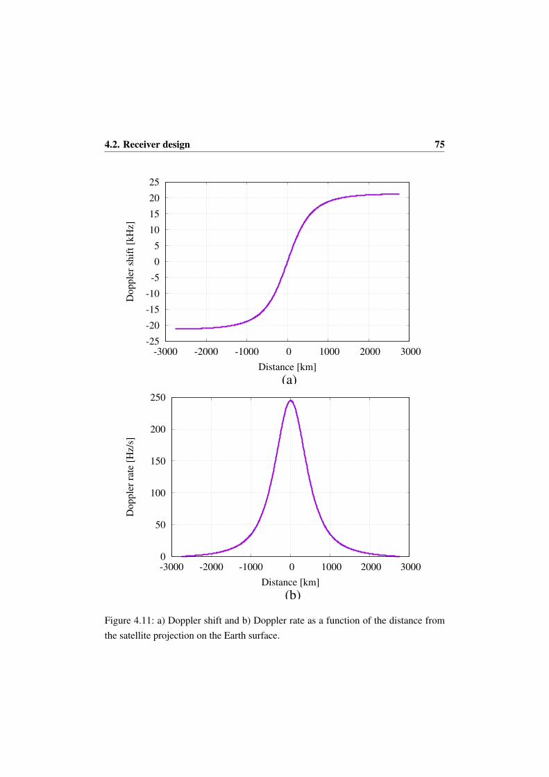
4.2. Receiver design 75
-25
-20
-15
-10
-5
0
5
10
15
20
25
-3000 -2000 -1000 0 1000 2000 3000
(a)
Dopple
r sh
ift
[kH
z]
Distance [km]
0
50
100
150
200
250
-3000 -2000 -1000 0 1000 2000 3000
(b)
Dopple
r ra
te [
Hz/
s]
Distance [km]
Figure 4.11: a) Doppler shift and b) Doppler rate as a function of the distance fromthe satellite projection on the Earth surface.

76 Chapter 4. LEO Satellite Receiver for LoRa Modulated Signals
10−3
10−2
10−1
100
11 11.5 12 12.5 13 13.5 14 14.5 15
PER
Es/N0 [dB]
Idealα = 33 Hz/sα = 99 Hz/sα = 132 Hz/sα = 165 Hz/s
10−2
10−1
100
12 12.5 13 13.5 14 14.5 15
PER
Es/N0 [dB]
Idealα = 2 Hz/sα = 4 Hz/sα = 6 Hz/sα = 8 Hz/sα = 10 Hz/sα = 12 Hz/s
Figure 4.12: PER performance in the presence of Doppler rate, with perfect compen-sation of timing and frequency offset, for SF = 10 on the left and SF = 12 on theright.
rate ~11 Hz/s yields a symbol shift by the end of the packet, even in the absence ofnoise). Hence, it is required to estimate the Doppler rate value with an accuracy of afew Hz/s. In the case SF = 10 instead, higher values of Doppler rate are required toworsen the performance.
There exist several algorithms for data-aided Doppler rate estimation. One of themost effective algorithms is that proposed in [65], and can be directly applied to thereceived signal once modulation and chirping have been removed, and timing andfrequency offset have been compensated for. However, when applied to our scenario,it does not provide the required accuracy. We investigated the performance of the al-gorithm in [65], applied in three different ways, all exploiting the received samplescorresponding to Ne =10 preamble symbols (8 up-chirp symbols and the 2 following“special” known symbols). The first approach (alg. #1), consisted in employing all10 symbols together and with optimized algorithm parameters (specifically, L = 256,see [65]). In the second algorithm we tested (alg. #2), we applied the algorithm 10times to the samples of each symbol and then we averaged over the 10 estimates. Inthe third approach, we averaged over 10 estimates computed by taking one sampleevery 10 from the whole sequence of samples corresponding to 10 symbols (alg. #3).Besides, we simulated an algorithm based on the Rife-Boorstyn technique to obtainthe estimates of the peak position on each symbol interval, and processed these dif-

4.2. Receiver design 77
ferent estimates (alg. #4). In other words, in this case we estimate the Doppler rate byobserving the position of the frequency peaks throughout the 10 preamble symbols.The peak values are then processed in order to find the linear regression which rep-resents the frequency increment due to Doppler rate. Nevertheless, the few availabledata suffer by a high incidence of outliers, which are partly due to the low SNR, butalso to the residual timing compensation error. A feasible solution, thus, is to furtherprocess the preamble samples, in order to reduce the impact of such outliers on theestimate. Basically, the estimation is performed on the 10 symbols (the down-chirpscannot be used because the unavoidable imperfect timing compensation leads to aphase shift with respect to the up-chirped symbols, which typically worsen the esti-mation), which are used in pairs to compute many different Doppler rate estimates,essentially two-point linear regressions, instead of computing a single linear regres-sion estimate using all 10 symbols; an average over these estimates turns out to havea better performance, since the effect of the outliers is more likely to be averagedout. Fig. 4.13 outlines the results in terms of square root of the Mean Square Esti-mation Error (MSEE), normalized to the sampling frequency, obtained by averagingover 10000 trials per SNR value, and assuming perfect timing and frequency offsetcompensation. The MCRLB is also reported for convenience. It is worth specifyingthat results do not change with the amount of the considered Doppler rate value. Wecan observe that, although algorithms 1 and 3 are able to reach the MCRLB, theystart converging for very high values of the signal-to-noise ratio. On the contrary, al-gorithm 4 remains quite far from the MCRLB but its convergence threshold is muchlower, around ~15 dB. Moreover, we should consider that, actually, algorithms #1and #3 turn out to be unreliable under non-ideal conditions, since the phase jumpsbetween adjacent symbols, due to imperfect timing compensation, severely affecttheir performance.
Finally, Fig. 4.14 shows the performance of the algorithm #4, for increasing num-ber of symbols Ne used for the estimation compared with the required minimum valueof the accuracy (~6 Hz/s, which was previously identified as a critical value). The ideahere is to use the decisions to improve the estimate accuracy in a decision-directedmode. Since, in any case, the performance of the estimators and the minimum value
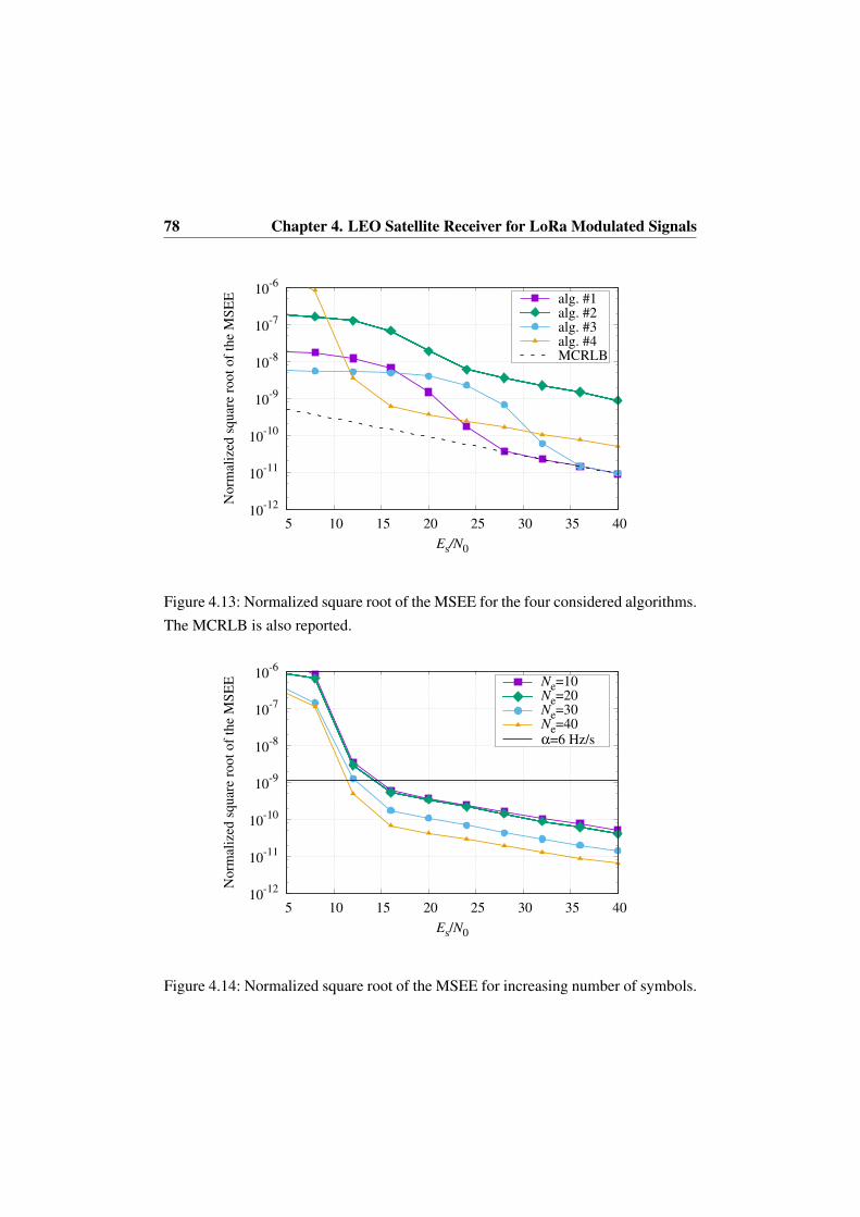
78 Chapter 4. LEO Satellite Receiver for LoRa Modulated Signals
10-12
10-11
10-10
10-9
10-8
10-7
10-6
5 10 15 20 25 30 35 40
No
rmal
ized
sq
uar
e ro
ot
of
the
MS
EE
Es/N0
alg. #1alg. #2alg. #3alg. #4MCRLB
Figure 4.13: Normalized square root of the MSEE for the four considered algorithms.The MCRLB is also reported.
10-12
10-11
10-10
10-9
10-8
10-7
10-6
5 10 15 20 25 30 35 40
No
rmal
ized
sq
uar
e ro
ot
of
the
MS
EE
Es/N0
Ne=10Ne=20Ne=30Ne=40α=6 Hz/s
Figure 4.14: Normalized square root of the MSEE for increasing number of symbols.
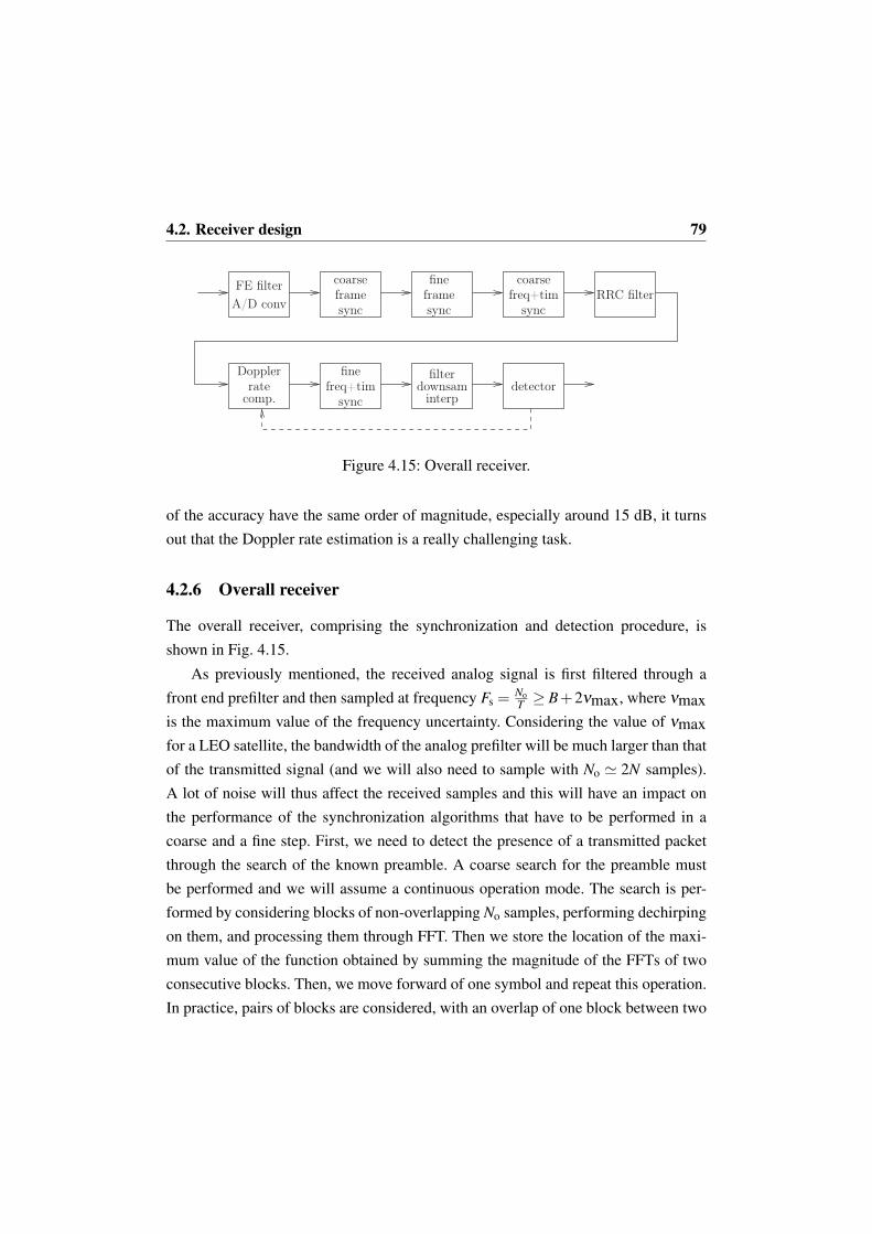
4.2. Receiver design 79
fineframesync
coarseframesync
coarsefreq+tim
sync
freq+timsync
fine filterdownsam
interp
FE filter
Dopplerrate
comp.
A/D convRRC filter
detector
Figure 4.15: Overall receiver.
of the accuracy have the same order of magnitude, especially around 15 dB, it turnsout that the Doppler rate estimation is a really challenging task.
4.2.6 Overall receiver
The overall receiver, comprising the synchronization and detection procedure, isshown in Fig. 4.15.
As previously mentioned, the received analog signal is first filtered through afront end prefilter and then sampled at frequency Fs =
NoT ≥ B+2νmax, where νmax
is the maximum value of the frequency uncertainty. Considering the value of νmaxfor a LEO satellite, the bandwidth of the analog prefilter will be much larger than thatof the transmitted signal (and we will also need to sample with No ' 2N samples).A lot of noise will thus affect the received samples and this will have an impact onthe performance of the synchronization algorithms that have to be performed in acoarse and a fine step. First, we need to detect the presence of a transmitted packetthrough the search of the known preamble. A coarse search for the preamble mustbe performed and we will assume a continuous operation mode. The search is per-formed by considering blocks of non-overlapping No samples, performing dechirpingon them, and processing them through FFT. Then we store the location of the maxi-mum value of the function obtained by summing the magnitude of the FFTs of twoconsecutive blocks. Then, we move forward of one symbol and repeat this operation.In practice, pairs of blocks are considered, with an overlap of one block between two

80 Chapter 4. LEO Satellite Receiver for LoRa Modulated Signals
consecutive pairs. When the maxima of 7 pairs of blocks are all in the same posi-tion on the FFT grid we are in the presence of 8 up-chirps. Two problems arise atthis point. As discussed, two peaks at distance B can be observed and, because ofthe noise, the maximum can “jump” between these peaks. Moreover, the Dopplerrate could increasingly shift the maxima throughout the preamble. Hence, instead oflooking for 7 consecutive peaks at the exact same position, we relax this constraint bylooking for less than 7 consecutive peaks, possibly not exactly at the same positionand possibly making “jumps” of B in their position. This is done to reduce the misseddetection probability since the false alarm probability is not a problem per sé. In fact,even if we erroneously identify a preamble, the verification of the Cyclic RedundancyCode (CRC) after detection will identify the absence of a valid packet.
The previous step is able to identify the presence of a packet but we will have asignificant uncertainty on its beginning. As a consequence, the receiver has to starta fine frame synchronization procedure. The aim of this procedure is to identify itsposition more precisely, and to reduce the uncertainty on the timing offset. This time,we take blocks of 10 consecutive symbols. Dechirping is performed by multiplyingthem by the complex conjugate of the first 10 symbols in the preamble. The magni-tude of the FFTs of these 10 symbols are computed, then summed, and both positionP and amplitude A of the maximum of the result are computed and stored. The win-dow containing these 10 symbols is then shifted of T/4 and the same operationsperformed over another block of 10 symbols, partially overlapped with the previousone. We iterate this procedure around the position returned by the coarse preamblesearch and keep the P corresponding to the largest stored value of the amplitude A.Now, the starting position of a packet is identified with an uncertainty lower thanT/4.
We can now perform coarse frequency and timing estimation. The position P ob-tained in the previous step will provide an estimate of either the frequency
(ν−B τ
T
)
or the frequency(B+ν−B τ
T
). By repeating the same operation on the two down-
chirp symbols we will obtain an estimate of either the frequency(ν +B τ
T
)or the
frequency(B+ν +B τ
T
). We now have to extract an estimate of both ν and τ , consid-
ering the ambiguity caused by the presence of two peaks and also taking into account

4.3. Numerical results 81
the cyclic nature of the FFT. Some of the possible pairs of ν and τ will correspond tovalues outside the allowed ranges. The remaining pairs can be disambiguated througha trial-and-error procedure, that consists in applying the compensation pair to an up-chirp block and then verifying if the maximum of its FFT is located in the zero (DC)tone (it is worth noting that it is not necessary to perform a whole FFT processing onthe symbol, but rather a processing on the tones around DC only).
After the coarse compensation of timing and frequency offset, a tight filteringcan be performed in order to reduce excess noise and improve the performance of thefollowing estimation steps. We used a filter with RRC amplitude and linear phase,with roll-off factor 0.06 and bandwidth B. At this stage, the Doppler rate estimationand compensation is performed.
Fine frequency and timing estimation is then performed. The algorithm is exactlythe same used in the coarse step, but this time we take advantage of the suppres-sion of the excess noise and of the Doppler rate compensation. After the estimation,the frequency shift is compensated, while fractional timing compensation and down-sampling to N samples can take place at the same time, through interpolation. Now,noncoherent detection can finally be performed, as described in Sec. 4.2.2.
The accuracy of the Doppler rate estimate should allow the detection of the firstNp payload symbols. We can use these Np symbols to refine the estimate and increasethe accuracy. So, we go compensate the Doppler rate with the new estimate, repeatthe fine frequency and timing synchronization, repeat the detection and, this time weuse the first 2Np symbols to refine the estimate. Thus, we repeat the procedure addingNp symbols at each iteration until the end of the packet is reached. We used Np = 5in our simulations.
4.3 Numerical results
We assessed the performance of the overall receiver through computer simulations.We considered the case of absence of interference (the performance in a more realis-tic scenario where interference takes place is considered in [3]). The results, in termsof PER versus the carrier-to-noise ratio C/N, i.e., the ratio between the signal and the

82 Chapter 4. LEO Satellite Receiver for LoRa Modulated Signals
10-3
10-2
10-1
100
-25 -20 -15 -10
PE
R
C/N [dB]
SF=7SF=8SF=9SF=10SF=11SF=12
Figure 4.16: PER performance in presence of random impairments (continuouslines), and with perfect estimation and compensation (dashed lines), for SF = 7÷12.
noise power, for different values of SF are reported in Fig. 4.16 and compared withthat of an ideal receiver which perfectly knows the channel parameters. We consid-ered packets of 50 symbols including the preamble and assumed that Doppler rateand Doppler shift take on the maximum possible values for the considered scenario.As mentioned, when SF = 12, the Doppler rate estimation and compensation is nec-essary (see previous sections for insights), and the penalty due to impairments canbe estimated as ~0.3 dB at a PER=10−2. The transmission of a signal with SF = 10instead can be considered as borderline, since the maximum Doppler rate can inducea symbol shift only after ~40 symbols. However, for values SF≤ 10, it seems betterto perform the Doppler rate estimation based on the uncompensated signal, at eachiteration of the decision-directed refinement process, rather than performing it on thesignal corrected in the previous iteration. This is due to errors in the estimation whenthere is only the small residual rate left.

4.4. Conclusions 83
4.4 Conclusions
The aim of this chapter was to design a receiver to extend the IoT LoRa networksthrough LEO satellites in remote areas. We described the LoRa modulation and pro-posed a design of a receiver that copes with the typical impairments of a LEO satellitelink. We saw that, being LoRa a frequency modulation, an uncompensated Dopplerrate is detrimental, especially for high values of the parameter SF . We thus proposeda receiver scheme that performs frame, timing, and frequency synchronization andalso removes the Doppler rate effects. The performance achieved by this receiver isalmost the same of an ideal AWGN channel, with small losses only for high valuesof SF .
This receiver has been used in a system simulator in [3]. It includes the inter-ference coming from all the users in the field of view of the satellite, the frequencyoffsets due to the oscillators instability and computes the Doppler rate, the Dopplershift, and the attenuation for each transmitting user. To achieve better results it alsomakes use of interference cancellation after the successful detection of a packet.


Conclusions
In this thesis we analyzed three different scenarios of satellite communications andproposed optimized transceivers for them.
We first investigated a single-carrier per transponder scenario. We proposed threeschemes for a cooperation among two receivers that communicate over a capacityconstrained side-channel. We derived a closed form of an MMSE based receiver, thatcan also be extended to the CS framework. Then we proposed a receiver based ona modification of the BCJR to accommodate for the presence of the side-channel.Lastly, we tested a scheme that quantizes the LLRs instead of the symbols. Weshowed a comparison of their performance from an information rate perspective de-pending on the capacity of the constrained link. We also confirmed the correspon-dence among information rate results and packet error rate simulations with standardMODCODs.
The second scenario was focused on satellites for Earth observation. We con-sidered two different configurations, when the satellite uses one or two separatedradio-frequency chains, and applied several transceiver techniques. We saw that anoptimization of the symbol rate can provide noticeable advantages with respect tothe reference system. Moreover, for the two channels configuration, we have com-pared classical single-user detection, multiuser detection, and the Alamouti scheme.We also discussed on the introduction of an IC-CS receiver for high symbol-rate.
Finally, we studied a LEO satellite receiver to extend LoRa-based IoT networks.We first introduced the fundamental aspects of the LoRa protocol and modulation.We showed that the typical challenges of a LEO satellite scenario (i.e., Doppler shift

86 Conclusions
and Doppler rate) have a huge impact on the performance of the LoRa modulation.Then, we proposed a receiver that could reliably receive LoRa signals in this scenario.It performs packet detection, frame synchronization, timing and frequency synchro-nization, and Doppler rate estimation and correction. Despite the number of impair-ments to take into account, we manage to reach a performance similar to that in anideal AWGN channel, where the only impairment is noise.

Bibliography
[1] ETSI EN 302 307-2 Digital Video Broadcasting (DVB), Second generationframing structure, channel coding and modulation systems for Broadcast-ing, Interactive Services, News Gathering and other broadband satellite ap-plications, Part II: S2-Extensions (DVB-S2X), Available on ETSI web site(http://www.etsi.org).
[2] O. B. A. Seller, et. al., “Low power long range transmitter,” 2014, EP PatentApp. EP20,131,154,071.
[3] Y. Zanettini, “Techniques for interference mitigation in satellite communica-tions,” Ph.D. dissertation, Università di Parma, 2017, PhD Thesis, University ofParma.
[4] T. M. Cover and J. A. Thomas, Elements of Information Theory, 2nd ed. NewYork: John Wiley & Sons, 2006.
[5] D. M. Arnold, H.-A. Loeliger, P. O. Vontobel, A. Kavcic, and W. Zeng,“Simulation-based computation of information rates for channels with mem-ory,” IEEE Trans. Inform. Theory, vol. 52, no. 8, pp. 3498–3508, Aug. 2006.
[6] L. R. Bahl, J. Cocke, F. Jelinek, and J. Raviv, “Optimal decoding of linear codesfor minimizing symbol error rate,” IEEE Trans. Inform. Theory, vol. 20, pp.284–287, Mar. 1974.

88 Bibliography
[7] N. Merhav, G. Kaplan, A. Lapidoth, and S. Shamai, “On information rates formismatched decoders,” IEEE Trans. Inform. Theory, vol. 40, no. 6, pp. 1953–1967, Nov. 1994.
[8] U. Fincke and M. Pohst, “Improved methods for calculating vectors of shortlength in a lattice, including a complexity analysis,” Mathematics of computa-tion, vol. 44, no. 170, pp. 463–471, Apr. 1985.
[9] J. Hagenauer and C. Kuhn, “Turbo equalization for channels with high memoryusing a list-sequential (liss) equalizer,” in Proc. International Symposium onTurbo Codes and Related Topics (ISTC’03), 2003.
[10] K. K. Y. Wong, The soft-output M-algorithm and its applications. Queen’sUniversity, 2006.
[11] D. D. Falconer and F. Magee, “Adaptive channel memory truncation for max-imum likelihood sequence estimation,” Bell System Tech. J., vol. 52, no. 9, pp.1541–1562, Nov. 1973.
[12] F. Rusek and A. Prlja, “Optimal channel shortening for MIMO and ISI chan-nels,” IEEE Trans. Wireless Commun., vol. 11, no. 2, pp. 810–818, Feb. 2012.
[13] S. Hu and F. Rusek, “On the design of channel shortening demodu-lators for iterative receivers in MIMO and ISI channels,” available athttp://arxiv.org/abs/1506.07331.
[14] ——, “On the design of reduced state demodulators with interference cancel-lation for iterative receivers,” in Proc. 24th IEEE Intern. Symp. on Personal,Indoor, and Mobile Radio Comm. (PIMRC), Hong Kong, China, Aug. 2015, pp.981–985.
[15] A. Modenini, F. Rusek, and G. Colavolpe, “Adaptive rate-maximizing channel-shortening for ISI channels,” IEEE Commun. Letters, vol. 19, no. 12, pp. 2090–2093, Dec. 2015.

Bibliography 89
[16] S. Haykin, Adaptive Filter Theory, 3rd ed. Englewood Cliffs, NJ: Prentice-Hall, 1996.
[17] A. Barbieri, D. Fertonani, and G. Colavolpe, “Improving the spectral efficiencyof linear modulations through time-frequency packing,” in Proc. IEEE Inter-national Symposium on Information Theory, Toronto, Canada, Jul. 2008, pp.2742–2746.
[18] P. Banelli, S. Buzzi, G. Colavolpe, A. Modenini, F. Rusek, and A. Ugolini,“Modulation formats and waveforms for 5G networks: Who will be the heir ofOFDM?” IEEE Signal Processing Mag., vol. 31, no. 6, pp. 80–93, Nov. 2014.
[19] G. Colavolpe and T. Foggi, “Time-frequency packing for high capacity coherentoptical links,” IEEE Trans. Commun., vol. 62, pp. 2986–2995, Aug. 2014.
[20] A. Modenini, G. Colavolpe, and N. Alagha, “How to significantly improve thespectral efficiency of linear modulations through time-frequency packing andadvanced processing,” in Proc. IEEE Intern. Conf. Commun., Ottawa, Canada,Jun. 2012, pp. 3299–3304.
[21] S. Khattak, W. Rave, and G. Fettweis, “Distributed iterative multiuserdetection through base station cooperation,” EURASIP Journal on WirelessCommunications and Networking, vol. 2008, no. 1, p. 390489, 2008. [Online].Available: http://dx.doi.org/10.1155/2008/390489
[22] ETSI EN 302 307-1 Digital Video Broadcasting (DVB), Second generationframing structure, channel coding and modulation systems for Broadcasting, In-teractive Services, News Gathering and other broadband satellite applications,Part I: DVB-S2, Available on ETSI web site (http://www.etsi.org).
[23] S. Cioni, G. Colavolpe, V. Mignone, A. Modenini, A. Morello, M. Ricciulli,A. Ugolini, and Y. Zanettini, “Transmission parameters optimization and re-ceiver architectures for DVB-S2X systems,” International Journal of SatelliteCommunications and Networking, vol. 34, pp. 337–350, May/June 2016, articlefirst published online: June 2015.

90 Bibliography
[24] A. Ugolini, A. Modenini, G. Colavolpe, V. Mignone, and A. Morello, “Ad-vanced techniques for spectrally efficient DVB-S2X systems,” InternationalJournal of Satellite Communications and Networking, vol. 34, pp. 609–623,Sep./Oct. 2016, article first published online: September 2015.
[25] H. Meyr, M. Oerder, and A. Polydoros, “On sampling rate, analog prefiltering,and sufficient statistics for digital receivers,” IEEE Trans. Commun., vol. 42, pp.3208–3214, Dec. 1994.
[26] G. Karam and H. Sari, “Analysis of predistortion, equalization, and ISI cancel-lation techniques in digital radio systems with nonlinear transmit amplifiers,”IEEE Trans. Commun., vol. 37, pp. 1245–1253, Dec 1989.
[27] E. Casini, R. De Gaudenzi, and A. Ginesi, “DVB-S2 modem algorithms designand performance over typical satellite channels,” Intern. J. of Satellite Commu-nications and Networking, vol. 22, no. 3, pp. 281–318, May/June 2004.
[28] V. Kostina and S. Verdú, “Nonasymptotic noisy lossy source coding,” IEEETransactions on Information Theory, vol. 62, no. 11, pp. 6111–6123, Nov 2016.
[29] J. M. Cioffi, G. P. Dudevoir, M. V. Eyuboglu, and G. D. Forney, “MMSEdecision-feedback equalizers and coding. I. Equalization results,” IEEE Trans.Commun., vol. 43, no. 10, pp. 2582–2594, Oct 1995.
[30] G. D. Forney, Jr., “Maximum-likelihood sequence estimation of digital se-quences in the presence of intersymbol interference,” IEEE Trans. Inform. The-ory, vol. 18, pp. 284–287, May 1972.
[31] G. Ungerboeck, “Adaptive maximum likelihood receiver for carrier-modulateddata-transmission systems,” IEEE Trans. Commun., vol. com-22, pp. 624–636,May 1974.
[32] S. Cioni, G. Colavolpe, C. Ernst, and A. Ginesi, “Bandwidth optimizationfor satellite digital broadcasting,” in 31st AIAA International CommunicationsSatellite Systems Conference, Florence, Italy, Oct. 2013.

Bibliography 91
[33] A. Ganti, A. Lapidoth, and I. E. Telatar, “Mismatched decoding revisited:General alphabets, channels with memory, and the wide-band limit,” IEEETrans. Inform. Theory, vol. 46, no. 7, pp. 2315–2328, Nov. 2000.
[34] G. Caire, G. Taricco, and E. Biglieri, “Bit-interleaved coded modulation,” IEEETrans. Inform. Theory, vol. 44, no. 3, pp. 927–946, May 1999.
[35] L. Ding, G. Zhou, D. Morgan, M. Zhengxiang, J. Kenney, K. Jaehyeong, andC. Giardina, “A robust digital baseband predistorter constructed using memorypolynomials,” IEEE Trans. on Commun., vol. 52, no. 1, pp. 159–165, Jan. 2004.
[36] N. Mazzali, B. Shankar, and B. Ottersten, “On-board signal predistortion fordigital transparent satellites,” in Proc. IEEE Intern. Work. on Signal ProcessingAdvances for Wireless Commun., Stockholm, Sweden, June-July 2015, pp. 535–539.
[37] N. Kelly, M. Allegue-Martínez, P.-D. Arapoglou, and A. Zhu, “Bandwidth-constrained digital pre-compensation technique for multi-carrier satellite com-munications,” International Journal of Satellite Communications and Network-ing, vol. 34, pp. 171–194, March/April 2016, article first published online: April2015.
[38] CCSDS 131.2-B-1, Flexible advanced coding and modulationscheme for high rate telemetry applications, Mar. 2012, Available athttp://public.ccsds.org/publications/BlueBooks.aspx.
[39] W. Cauer, Synthesis of linear communication networks, 2nd ed. New York:McGraw–Hill, 1958.
[40] J. E. Mazo, “Faster-than-Nyquist signaling,” Bell System Tech. J., vol. 54, pp.1450–1462, Oct. 1975.
[41] J. E. Mazo and H. J. Landau, “On the minimum distance problem for faster-than-Nyquist signaling,” IEEE Trans. Inform. Theory, pp. 1420–1427, Nov.1988.

92 Bibliography
[42] A. Liveris and C. N. Georghiades, “Exploiting faster-than-Nyquist signaling,”IEEE Trans. Commun., vol. 47, pp. 1502–1511, Sep. 2003.
[43] F. Rusek and J. B. Anderson, “The two dimensional Mazo limit,” in Proc. IEEEInternational Symposium on Information Theory, Adelaide, Australia, Nov.2005, pp. 970–974.
[44] A. Barbieri, D. Fertonani, and G. Colavolpe, “Time-frequency packing for lin-ear modulations: spectral efficiency and practical detection schemes,” IEEETrans. Commun., vol. 57, pp. 2951–2959, Oct. 2009.
[45] A. Piemontese, A. Modenini, G. Colavolpe, and N. Alagha, “Improving thespectral efficiency of nonlinear satellite systems through time-frequency pack-ing and advanced processing,” IEEE Trans. Commun., vol. 61, no. 8, pp. 3404–3412, Aug. 2013.
[46] S. Verdú, Multiuser Detection. Cambridge, UK: Cambridge University Press,1998.
[47] S. M. Alamouti, “A simple transmit diversity technique for wireless communi-cations,” IEEE J. Select. Areas Commun., vol. 16, no. 8, pp. 1451–1458, Oct.1998.
[48] A. Modenini, A. Ugolini, A. Piemontese, and G. Colavolpe, “On the use ofmultiple satellites to improve the spectral efficiency of broadcast transmissions,”IEEE Trans. Broadcast., vol. 61, no. 4, pp. 590–602, Dec. 2015.
[49] M. J. D. Powell, “The BOBYQA algorithm for bound constrained optimiza-tion without derivatives,” Department of Applied Mathematics and TheoreticalPhysics, Cambridge, England, Tech. Rep., Aug. 2009.
[50] S. G. Johnson, “The NLopt nonlinear-optimization package,” http://ab-initio.mit.edu/nlopt.
[51] G. Colavolpe, A. Modenini, A. Piemontese, and A. Ugolini, “Multiuser detec-tion in multibeam satellite systems: Theoretical analysis and practical schemes,”

Bibliography 93
in Proc. IEEE Intern. Work. on Signal Processing Advances for Wireless Com-mun., Stockholm, Sweden, June-July 2015, pp. 525–529.
[52] M. Witzke, S. Baro, F. Schreckenbach, and J. Hagenauer, “Iterative detection ofmimo signals with linear detectors,” in Conference Record of the Thirty-SixthAsilomar Conference on Signals, Systems and Computers, 2002., vol. 1, Nov2002, pp. 289–293 vol.1.
[53] C. Studer, S. Fateh, and D. Seethaler, “Asic implementation of soft-input soft-output mimo detection using mmse parallel interference cancellation,” IEEEJournal of Solid-State Circuits, vol. 46, no. 7, pp. 1754–1765, July 2011.
[54] J. Zhang, H. Nguyen, and G. Mandyam, “Lmmse-based iterative and turboequalization methods for cdma downlink channels,” in IEEE 6th Workshop onSignal Processing Advances in Wireless Communications, 2005., June 2005, pp.231–235.
[55] LoRa Alliance, Inc., “LoRaWAN Specification,” Jul. 2016.
[56] S. G. Wilson, Digital Modulation and Coding. Prentice Hall, 1996.
[57] I. S. Gradshtein and I. M. Ryzhik, Table of Integrals, Series and Products. NewYork: Academic Press, 1980.
[58] A. Papoulis, Probability, Random Variables and Stochastic Processes. NewYork, NY: McGraw-Hill, 1991.
[59] S. Benedetto and E. Biglieri, Principles of Digital Transmission: With WirelessApplications. Norwell, MA, USA: Kluwer Academic Publishers, 1999.
[60] G. Colavolpe and R. Raheli, “Theoretical analysis and performance limits ofnoncoherent sequence detection of coded PSK,” IEEE Trans. Inform. Theory,vol. 46, no. 4, pp. 1483–1494, Jul. 2000.
[61] D. C. Rife and R. R. Boorstyn, “Single tone parameter estimation from discrete-time observations,” IEEE Trans. Inform. Theory, vol. 20, pp. 591–598, Septem-ber 1974.

94 Bibliography
[62] U. Mengali and M. Morelli, “Data-aided frequency estimation for burst digitaltransmission,” IEEE Trans. Commun., vol. 45, pp. 23–25, Jan. 1997.
[63] A. N. D’Andrea, U. Mengali, and R. Reggiannini, “The modified Cramer-Raobound and its application to synchronization problems,” IEEE Trans. Commun.,vol. 42, pp. 1391–1399, Feb. 1994.
[64] I. Ali, N. Al-Dhahir, and J. E. Hershey, “Doppler characterization for LEO satel-lites,” IEEE Trans. Commun., vol. 46, pp. 309–313, Mar. 1998.
[65] M. Morelli, “Doppler-rate estimation for burst digital transmission,” IEEETrans. Commun., vol. 50, pp. 707–710, May 2002.

Acknowledgements
The list of people that helped me during the last three years is fairly long and Iam hoping I am not forgetting anyone. The first person to thank is my tutor, Giulio.Firstly, because he believed in me and took me in his research group. But also forthe help, the insightful discussions, the guidance throughout the PhD and the hugeamount of patience. Then, it is natural to thank the whole SpadicLab. Alessandro,Andrea (for a short period), Tommy and Yuri have been the best team one couldthink of. They helped me anytime I asked for advice, and taught me a lot. Really alot! Yuri deserves a special “thank you”, since he started this adventure with me andwe spent three years in the same office: needless to say, we also shared a lot of laughs,a lot of work, a lot of food and a lot of coffees. Thanks for all the suggestions, the helpyou gave me and all the “Michelangelo, ti sei ricordato di consegnare i documenti insegreteria?”. (And thanks of course for the best memes on Whatsapp!)
Talking about coffee, I need to thank Matteo and Simone, for all the coffees, thematched-betting and especially for their “fair” monetary loans.

96 Acknowledgements
It is time to move abroad now. During my experience in Lund University, Sweden,I met a group of very nice and smart people that made me feel welcome from thevery beginning. I quickly became part of the group and had the impression that notonly we were “on the same wavelength”, but we were probably also using the samemodulation scheme. First I want to thank Fredrik for his advice, for his time andfor accepting the burden of my presence in Lund University. In only two months hetaught me a lot about information theory, telecommunications and Swedish culture.Then, I thank Dimitrios, Muris, João and Zach for their friendliness, for the beers,the fika and the insightful discussions about life at Medicon and Rosegarden. I alsowant to thank Husha for his kindness and helpfulness.
Of course, I cannot forget to thank my closest friends and my brothers ( there’s noneed to make a list, they know who they are). Their company and the laughs I sharedwith them are among the things that gave me strength and joy even in the darkestmoments. It’s not a coincidence I put friends and brothers in the same paragraph.
Grazie a mia madre e a mio padre. Per il loro supporto e per tutto ciò che mihanno insegnato. Non sarei arrivato nè a questa, nè alle altre tesi senza la loro guida.
Last but not least, thanks Valeria. Thanks for the patience you showed and every-thing you did for me. I could write a list of the reasons, but it would be longer thanthe thesis itself. And it would probably not be sufficient, anyway.
Michelangelo