advancements in finite element methods for newtonian …rebholz/keithgalvin_phdthesis.pdf ·...
TRANSCRIPT
Advancements in finite element methods for Newtonianand non-Newtonian flows
A Dissertation
Presented to
the Graduate School of
Clemson University
In Partial Fulfillment
of the Requirements for the Degree
Doctor of Philosophy
Mathematical Sciences
by
Keith J. Galvin
August 2013
Accepted by:
Dr. Hyesuk Lee, Committee Chair
Dr. Leo Rebholz, Co-Chair
Dr. Chris Cox
Dr. Vincent Ervin

Abstract
This dissertation studies two important problems in the mathematics of computational
fluid dynamics. The first problem concerns the accurate and efficient simulation of incompressible,
viscous Newtonian flows, described by the Navier-Stokes equations. A direct numerical simulation
of these types of flows is, in most cases, not computationally feasible. Hence, the first half of
this work studies two separate types of models designed to more accurately and efficient simulate
these flows. The second half focuses on the defective boundary problem for non-Newtonian flows.
Non-Newtonian flows are generally governed by more complex modeling equations, and the lack of
standard Dirichlet or Neumann boundary conditions further complicates these problems. We present
two different numerical methods to solve these defective boundary problems for non-Newtonian flows,
with application to both generalized-Newtonian and viscoelastic flow models.
Chapter 3 studies a finite element method for the 3D Navier-Stokes equations in velocity-
vorticity-helicity formulation, which solves directly for velocity, vorticity, Bernoulli pressure and
helical density. The algorithm presented strongly enforces solenoidal constraints on both the veloc-
ity (to enforce the physical law for conservation of mass) and vorticity (to enforce the mathematical
law that div(curl)= 0). We prove unconditional stability of the velocity, and with the use of a
(consistent) penalty term on the difference between the computed vorticity and curl of the com-
puted velocity, we are also able to prove unconditional stability of the vorticity in a weaker norm.
Numerical experiments are given that confirm expected convergence rates, and test the method on
a benchmark problem.
Chapter 4 focuses on one main issue from the method presented in Chapter 3, which is
the question of appropriate (and practical) vorticity boundary conditions. A new, natural vorticity
boundary condition is derived directly from the Navier-Stokes equations. We propose a numeri-
cal scheme implementing this new boundary condition to evaluate its effectiveness in a numerical
ii

experiment.
Chapter 5 derives a new, reduced order, multiscale deconvolution model. Multiscale decon-
volution models are a type of large eddy simulation models, which filter out small energy scales and
model their effect on the large scales (which significantly reduces the amount of degrees of freedom
necessary for simulations). We present both an efficient and stable numerical method to approximate
our new reduced order model, and evaluate its effectiveness on two 3d benchmark flow problems.
In Chapter 6 a numerical method for a generalized-Newtonian fluid with flow rate boundary
conditions is considered. The defective boundary condition problem is formulated as a constrained
optimal control problem, where a flow balance is forced on the inflow and outflow boundaries using
a Neumann control. The control problem is analyzed for an existence result and the Lagrange
multiplier rule. A decoupling solution algorithm is presented and numerical experiments are provided
to validate robustness of the algorithm.
Finally, this work concludes with Chapter 7, which studies two numerical algorithms for
viscoelastic fluid flows with defective boundary conditions, where only flow rates or mean pres-
sures are prescribed on parts of the boundary. As in Chapter 6, the defective boundary condition
problem is formulated as a minimization problem, where we seek boundary conditions of the flow
equations which yield an optimal functional value. Two different approaches are considered in devel-
oping computational algorithms for the constrained optimization problem, and results of numerical
experiments are presented to compare performance of the algorithms.
iii

Table of Contents
Title Page . . . . . . . . . . . . . . . . . . . . . . . . . . . . . . . . . . . . . . . . . . . . i
Abstract . . . . . . . . . . . . . . . . . . . . . . . . . . . . . . . . . . . . . . . . . . . . . ii
List of Tables . . . . . . . . . . . . . . . . . . . . . . . . . . . . . . . . . . . . . . . . . . vi
List of Figures . . . . . . . . . . . . . . . . . . . . . . . . . . . . . . . . . . . . . . . . . . vii
1 Introduction . . . . . . . . . . . . . . . . . . . . . . . . . . . . . . . . . . . . . . . . . 1
2 Preliminaries . . . . . . . . . . . . . . . . . . . . . . . . . . . . . . . . . . . . . . . . . 10
3 A Numerical Study for a Velocity-Vorticity-Helicity formulation of the 3DTime-Dependent NSE . . . . . . . . . . . . . . . . . . . . . . . . . . . . . . . . . . . 163.1 Discrete VVH Formulation . . . . . . . . . . . . . . . . . . . . . . . . . . . . . . . . 173.2 Numerical Results . . . . . . . . . . . . . . . . . . . . . . . . . . . . . . . . . . . . . 25
4 Natural vorticity boundary conditions for coupled vorticity equations . . . . . . 304.1 Derivation . . . . . . . . . . . . . . . . . . . . . . . . . . . . . . . . . . . . . . . . . . 304.2 Numerical Results . . . . . . . . . . . . . . . . . . . . . . . . . . . . . . . . . . . . . 32
5 A New Reduced Order Multiscale Deconvolution Model . . . . . . . . . . . . . . 355.1 Derivation . . . . . . . . . . . . . . . . . . . . . . . . . . . . . . . . . . . . . . . . . . 355.2 The Discrete Setting . . . . . . . . . . . . . . . . . . . . . . . . . . . . . . . . . . . . 375.3 Error Analysis . . . . . . . . . . . . . . . . . . . . . . . . . . . . . . . . . . . . . . . 435.4 Numerical Results . . . . . . . . . . . . . . . . . . . . . . . . . . . . . . . . . . . . . 56
6 Analysis and approximation of the Cross model for quasi-Newtonian flows withdefective boundary conditions . . . . . . . . . . . . . . . . . . . . . . . . . . . . . . 626.1 Modeling Equations and Preliminaries . . . . . . . . . . . . . . . . . . . . . . . . . . 636.2 The Optimal Control Problem . . . . . . . . . . . . . . . . . . . . . . . . . . . . . . 656.3 The Optimality System . . . . . . . . . . . . . . . . . . . . . . . . . . . . . . . . . . 666.4 Steepest descent approach . . . . . . . . . . . . . . . . . . . . . . . . . . . . . . . . . 726.5 Numerical Results . . . . . . . . . . . . . . . . . . . . . . . . . . . . . . . . . . . . . 74
7 Approximation of viscoelastic flows with defective boundary conditions . . . . . 797.1 Model equations . . . . . . . . . . . . . . . . . . . . . . . . . . . . . . . . . . . . . . 797.2 The Optimality system . . . . . . . . . . . . . . . . . . . . . . . . . . . . . . . . . . . 817.3 Steepest descent approach . . . . . . . . . . . . . . . . . . . . . . . . . . . . . . . . . 837.4 Mean pressure boundary condition . . . . . . . . . . . . . . . . . . . . . . . . . . . . 857.5 Nonlinear least squares approach . . . . . . . . . . . . . . . . . . . . . . . . . . . . . 867.6 Numerical Results . . . . . . . . . . . . . . . . . . . . . . . . . . . . . . . . . . . . . 90
iv

8 Conclusions . . . . . . . . . . . . . . . . . . . . . . . . . . . . . . . . . . . . . . . . . 99
Appendices . . . . . . . . . . . . . . . . . . . . . . . . . . . . . . . . . . . . . . . . . . . 101A deal.II code for 3d vorticity equation . . . . . . . . . . . . . . . . . . . . . . . . . . . 102
Bibliography . . . . . . . . . . . . . . . . . . . . . . . . . . . . . . . . . . . . . . . . . . . 151
v

List of Tables
3.1 Velocity and Vorticity errors and convergence rates using the nodal interpolant of thetrue vorticity for the vorticity boundary condition. . . . . . . . . . . . . . . . . . . . 26
3.2 Velocity and Vorticity errors and convergence rates using the nodal interpolant of theL2 projection of the curl of the discrete velocity into Vh, for the vorticity boundarycondition. . . . . . . . . . . . . . . . . . . . . . . . . . . . . . . . . . . . . . . . . . . 27
3.3 Velocity and Vorticity errors and convergence rates using nodal averages of the curlof the discrete velocity for the vorticity boundary condition. . . . . . . . . . . . . . . 27
4.1 Velocity errors and convergence rates for the first 3d numerical experiment . . . . . 344.2 Vorticity errors and convergence rates for the first 3d numerical experiment . . . . . 34
vi
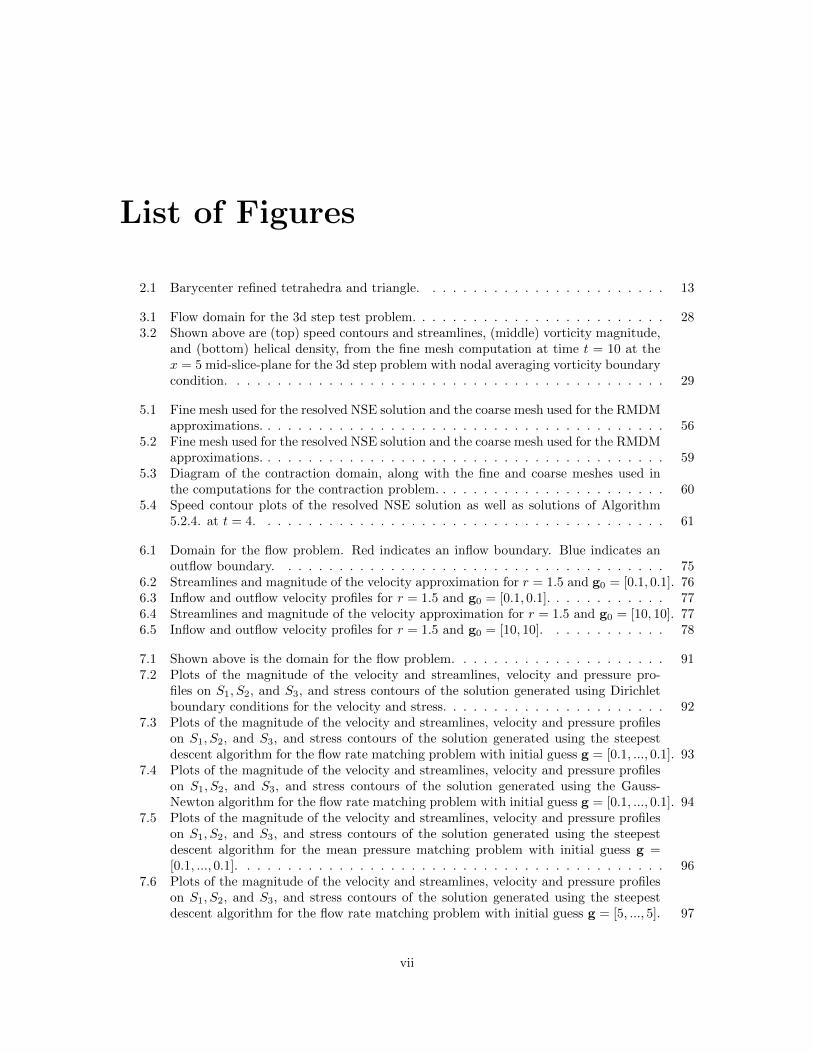
List of Figures
2.1 Barycenter refined tetrahedra and triangle. . . . . . . . . . . . . . . . . . . . . . . . 13
3.1 Flow domain for the 3d step test problem. . . . . . . . . . . . . . . . . . . . . . . . . 283.2 Shown above are (top) speed contours and streamlines, (middle) vorticity magnitude,
and (bottom) helical density, from the fine mesh computation at time t = 10 at thex = 5 mid-slice-plane for the 3d step problem with nodal averaging vorticity boundarycondition. . . . . . . . . . . . . . . . . . . . . . . . . . . . . . . . . . . . . . . . . . . 29
5.1 Fine mesh used for the resolved NSE solution and the coarse mesh used for the RMDMapproximations. . . . . . . . . . . . . . . . . . . . . . . . . . . . . . . . . . . . . . . . 56
5.2 Fine mesh used for the resolved NSE solution and the coarse mesh used for the RMDMapproximations. . . . . . . . . . . . . . . . . . . . . . . . . . . . . . . . . . . . . . . . 59
5.3 Diagram of the contraction domain, along with the fine and coarse meshes used inthe computations for the contraction problem. . . . . . . . . . . . . . . . . . . . . . . 60
5.4 Speed contour plots of the resolved NSE solution as well as solutions of Algorithm5.2.4. at t = 4. . . . . . . . . . . . . . . . . . . . . . . . . . . . . . . . . . . . . . . . 61
6.1 Domain for the flow problem. Red indicates an inflow boundary. Blue indicates anoutflow boundary. . . . . . . . . . . . . . . . . . . . . . . . . . . . . . . . . . . . . . 75
6.2 Streamlines and magnitude of the velocity approximation for r = 1.5 and g0 = [0.1, 0.1]. 766.3 Inflow and outflow velocity profiles for r = 1.5 and g0 = [0.1, 0.1]. . . . . . . . . . . . 776.4 Streamlines and magnitude of the velocity approximation for r = 1.5 and g0 = [10, 10]. 776.5 Inflow and outflow velocity profiles for r = 1.5 and g0 = [10, 10]. . . . . . . . . . . . 78
7.1 Shown above is the domain for the flow problem. . . . . . . . . . . . . . . . . . . . . 917.2 Plots of the magnitude of the velocity and streamlines, velocity and pressure pro-
files on S1, S2, and S3, and stress contours of the solution generated using Dirichletboundary conditions for the velocity and stress. . . . . . . . . . . . . . . . . . . . . . 92
7.3 Plots of the magnitude of the velocity and streamlines, velocity and pressure profileson S1, S2, and S3, and stress contours of the solution generated using the steepestdescent algorithm for the flow rate matching problem with initial guess g = [0.1, ..., 0.1]. 93
7.4 Plots of the magnitude of the velocity and streamlines, velocity and pressure profileson S1, S2, and S3, and stress contours of the solution generated using the Gauss-Newton algorithm for the flow rate matching problem with initial guess g = [0.1, ..., 0.1]. 94
7.5 Plots of the magnitude of the velocity and streamlines, velocity and pressure profileson S1, S2, and S3, and stress contours of the solution generated using the steepestdescent algorithm for the mean pressure matching problem with initial guess g =[0.1, ..., 0.1]. . . . . . . . . . . . . . . . . . . . . . . . . . . . . . . . . . . . . . . . . . 96
7.6 Plots of the magnitude of the velocity and streamlines, velocity and pressure profileson S1, S2, and S3, and stress contours of the solution generated using the steepestdescent algorithm for the flow rate matching problem with initial guess g = [5, ..., 5]. 97
vii

7.7 Plots of the magnitude of the velocity and streamlines, velocity and pressure profileson S1, S2, and S3, and stress contours of the solution generated using the Gauss-Newton algorithm for the flow rate matching problem with initial guess g = [5, ..., 5]. 98
viii
Chapter 1
Introduction
The understanding of fluid flow has been a subject of scientific interest for hundreds of
years. More recently, the branch of fluid mechanics known as computational fluid dynamics (CFD)
has been an area of intense interest for mathematicians due to the multitude of scientific areas that
depend on it. Many industries (e.g. automotive, aerospace, environmental) rely on both accurate
and efficient simulations of various types of fluids. However, state of the art models and methods
are far from being able to efficiently solve most problems of interest in CFD to a desired degree
of precision. Moore’s law states (roughly) that the amount of computing power available doubles
every two years, and has proven to be a fairly accurate estimate over the last 50 years. Despite
the great advances made in computing power in that time period, and even assuming Moore’s law
for computational speed increase continues, the accurate and timely simulation of most flows will
not be achieved in the foreseeable future. Advances in mathematics for CFD have gained far more
towards this goal than computing power, by developing robust and efficient algorithms built on solid
mathematical and physical grounds.
It is the goal of this work to extend the state of the art in mathematics of CFD for two
important problems. The first concerns the accurate and efficient simulation of incompressible,
viscous Newtonian fluids. We will present and analyze a new numerical method for approximating
solutions to the velocity-vorticity-helicity formulation of the Navier-Stokes equations. The driving
force behind this new method is that it offers increased physical fidelity and numerical accuracy,
along with a step towards further understanding the important but ill-understood physical quantity
helicity. Discussion of this method naturally raises the very difficult question of how to accurately
1

impose boundary conditions on the vorticity, as well as how to compute with turbulent flows. For
the former, we propose a new natural boundary condition for the vorticity equation which increases
both the accuracy and physical relevance of our discrete vorticity approximation. For the latter, we
consider a new reduced-order multiscale model for simulating Newtonian fluids.
The second main problem we study in this work concerns the robust simulation of non-
Newtonian fluids in the absence of standard boundary conditions. This problem often arises when
modeling flow in an unbounded domain (e.g. modeling blood flow in a portion of a blood vessel). We
consider two different approaches for developing accurate and efficient methods for these “defective-
boundary” problems for non-Newtonian flows. The first, a gradient-descent method, is presented
and tested for both generalized-Newtonian and viscoelastic flow models, and analyzed in the case of
the former. The second, a nonlinear least squares method, is presented and tested on a viscoelastic
flow model.
The flow of time-dependent, incompressible, viscous Newtonian flows is modeled by the
Navier-Stokes equations (NSE), which may be derived from the continuity equation (describing
conservation of mass) and the equation describing conservation of momentum. In dimensionless
form, the NSE are formulated as
∂u
∂t− ν∆u + u · ∇u +∇p = f , (1.1)
∇ · u = 0, (1.2)
where u and p denote the fluid velocity and pressure, respectively, f denotes an external body force,
and ν > 0 denotes the fluid’s kinematic viscosity. The Reynolds number Re = ν−1 is a dimensionless
parameter representing the ratio of inertial forces to viscous forces. In laminar flows, which are
characterized by low Reynolds number, viscous forces dominate inertial forces, making the flow
field smooth. Simulations of laminar flows can often be performed without too much complication.
For flows with moderate Reynolds numbers, inertial forces start to play a larger role, resulting in
complex flow behaviors, making predictions much more difficult. Turbulent flows, characterized by
high Reynolds numbers, present very complex and chaotic flow properties, often requiring special
models and methods.
In 2010, a velocity-vorticity-helicity (VVH) formulation of the NSE was presented in [55].
This formulation was derived by taking the curl of mass and momentum equations (1.1)-(1.2), and
2

applying several vector identities to produce the vorticity-helical density equations
∂w
∂t− ν∆w + 2D(w)u−∇η = ∇× f , (1.3)
∇ ·w = 0. (1.4)
where w := ∇×u is the fluid vorticity, η := u·w is the helical density, and D(w) := 12 (∇w+(∇w)T )
is the symmetric part of the vorticity gradient. The dimensionless VVH formulation of the NSE
then comes from coupling (1.3)-(1.4) to the NSE via the rotational form of the nonlinearity in the
momentum equation
∂u
∂t− ν∆u + w × u +∇P = f , (1.5)
∇ · u = 0, (1.6)
∂w
∂t− ν∆w + 2D(w)u−∇η = ∇× f , (1.7)
∇ ·w = 0. (1.8)
Here P := 12u · u + ∇p denotes the Bernoulli pressure, which is needed because of our use of the
rotational form of the nonlinearity. Since its original derivation in 2010, VVH has been studied
in other applications including numerical methods for solving steady incompresible flow [50], the
Boussinesq equations [54], and as a selection criterion for the filtering radius in the NS-ω turbulence
model [51], all with excellent results.
The VVH formulation of the NSE has four important characteristics that make it attractive
for use in simulations. First, numerical methods based on finding velocity and vorticity tend to be
more accurate (usually for an added cost, but not necessarily with VVH) [62, 63, 59, 61, 52], and
especially in the boundary layer [17]. Second, it solves directly for the helical density η, which may
give insight into the important but ill-understood quantity helicity, H =∫
Ωη dx, which is believed
to play a fundamental role in turbulence [4, 53, 25, 9, 13, 12, 20, 19]. VVH is the first formulation to
directly solve for this helical quantity. Third, the use of ∇η in the vorticity equation enables η to act
as a Lagrange multiplier corresponding to the divergence-free constraint for the vorticity, analogous
to how the pressure relates to the conservation of mass equation. VVH is the first velocity-vorticity
method to naturally enforce incompressibility of the vorticity, which is important since (1.4) is as
3

much a mathematical constraint as it is a physical one, making its violation inconsistent on multiple
levels. Finally, the structure of the VVH system allows for a natural splitting of the system into a
two-step linearization, since lagging vorticity in the velocity equation linearizes the equation, and
similarly lagging velocity in the vorticity equation linearizes this equation as well. A numerical
method based on such a splitting was proposed in [55], and when coupled with a finite element
discretization, was shown to be accurate on some simple test problems. Chapter 3 of this work
will precisely define and further study this discretization of the VVH formulation of the NSE by
providing a rigorous stability analysis (for both velocity and vorticity), and testing the method on
a benchmark problem.
Amidst our study of this discretization of the VVH formulation, an important, but difficult
question is raised in regards to boundary conditions for the vorticity. Consider the basic vorticity
equation, derived by taking the curl of the momentum equation (1.1),
∂w
∂t− ν∆w + u · ∇w −w · ∇u = ∇× f . (1.9)
Perhaps the most natural and reasonable boundary condition for the vorticity is
w = ∇× u on ∂Ω. (1.10)
Unfortunately, this boundary condition presents some difficulty when employed with finite elements.
In general, differentiating the piecewise-polynomial uh can often lead to a decrease in convergence
order [50]. Recently, various methods for avoiding this loss in accuracy have been proposed. In
[62], a finite difference approximation of (1.10) using nodal values of the finite element functions
is employed. This method is fairly successful on uniform meshes when second-order accuracy is
desired, however, it’s implementation on non-uniform meshes and for higher-order elements can be
quite complex. In general, in the presence of sharp boundary layers of the velocity (e.g. for flows with
moderate or high Re), the use of the vorticity boundary condition (1.10) may require extreme mesh
refinement around the boundary to avoid inaccurate vorticity approximations. Other methodologies
for implementing vorticity boundary conditions have also been tried, with some success. In [55],
the vorticity on the boundary was set to be the L2 projection of the discontinuous finite element
function ∇× uh into the continuous finite element space. This method is one of three implemented
4
in the numerical testing of our method for the VVH system presented in Chapter 3, providing fairly
accurate results on a benchmark flow problem. Other strategies include using the boundary element
method [42], or the lattice Boltzmann method [18]. In Chapter 4, we employ a different approach
in deriving a new vorticity boundary condition, in hopes of avoiding any unnecessary complication.
The proposed method includes natural boundary conditions for a weak formulation of the vorticity
equation. The boundary conditions are derived directly from the physical equations and the finite
element method, making them simpler to understand than some of the aforementioned strategies.
A full derivation of these vorticity boundary conditions will be presented in Chapter 4, along with
a numerical scheme to evaluate their effectiveness in a numerical experiment.
Another clear need in the development of the VVH algorithm is for some kind of stabiliza-
tion/subgrid model to allow us to handle higher Re flows. In Chapter 5 we consider a new reduced
order, multiscale, approximate deconvolution model for Newtonian flows. Approximate deconvo-
lution models (ADM) are a form of large eddy simulation (LES) models introduced in [2, 3] for
the purpose of simulating large-scale flow strctures at a reduced computational cost compared with
direct numerical simulation (DNS). We know from Kolmogorov’s 1941 theory that eddies below a
critical size (O(Re−3/4) for 3d flow) are dominated by viscous forces and disappear very quickly,
while those above this critical size are deterministic in nature. Hence, a DNS requires O(Re9/4)
mesh points in space per time step to accurately simulate eddies in 3d. Even for moderate Re flows,
this requirement makes DNS computationally infeasible. ADM models (and LES models in general)
aim to avoid this problem by filtering out small scales, while modeling their effect on the large scales.
Because only large scales are being solved for, these models require a significantly smaller amount
of mesh points than DNS. Recently, a promising new multiscale deconvolution model (MDM) [22]
has been proposed which avoids some of the drawbacks of general ADM models, and is given by
vt +Gγv · ∇Gγv +∇q − ν∆v = f (1.11)
∇ · v = 0. (1.12)
This formulation makes use of two different Helmholtz filters (associated with two different filtering
radii α and γ) and a deconvolution operator Gγ which connects the two filter scales. This formulation
and these filters and operators will all be defined in detail in Chapter 5, where we derive (in detail)
a new, reduced order MDM, along with an efficient and stable algorithm to approximate it.
5

The second half of this work is concerned with the accurate and efficient simulation of the
defective boundary problem for two types of non-Newtonian fluids. The modeling of flow in an
unbounded domain requires the introduction of artificial boundaries. Often, the flow is assumed to
satisfy some Dirichlet or Neumann boundary condition on a portion of these artificial boundaries
(e.g. inflow or outflow boundaries). However, the amount of boundary data available for a given
flow is often very limited, making these types of boundary conditions very hard to impose. In many
practical applications the only flow data available are quantitative (e.g. average flow rates, mean
pressure values, etc.). In situations like these, it is often more realistic to model the flow using
defective boundary conditions. Typically, governing equations are chosen depending on the flow
being modeled, and instead of completing these equations with standard Dirichlet or Neumann type
boundary conditions, the defective boundary problem consists of only considering information such
as flow rates (or mean pressure values) on the inflow or outflow boundaries Si, i.e.
∫Si
u · n dS = Qi for i = 1, ...,m. (1.13)
We note that these boundary conditions are known as “defective” because they are insufficient to
close the differential model (i.e. our flow problem is ill-posed) [26]. The goal of the second half
of this work is to study this problem in the context of two different types of flows (and hence two
different types of modeling equations).
Before we proceed we note that flow problems with defective boundary conditions have been
studied in various applications in the past. In [41], the defective boundary problem for the NSE was
studied where flow rates are specified on inflow and outflow boundaries. In this work a “do-nothing”
approach is presented where the flow rate conditions are implicitly incorporated into the variational
formulation through the choice of appropriate boundary conditions and function spaces, resulting
in a well-posed variational problem. An alternative approach to the defective boundary problem for
the NSE subject to flow rate conditions was presented in [26]. In this study, the flow rate conditions
are enforced weakly via the Lagrange multiplier method. In [24] the defective boundary problem for
quasi-Newtonian flows subject to flow rate conditions was investigated using the Lagrange multiplier
method. Both the continuous and discrete variational formulations of a generalized set of modeling
equations were proven to be well-posed, and error analysis of the numerical approximation was also
presented. In [27], a new approach to the defective boundary problem for Stokes flow was proposed.
6

This approach formulates the defective boundary problem as an optimal control problem through the
choice of a suitable functional to minimize. This approach proved to be versatile, as the functional to
minimize can be altered to match various kinds of defective boundaries (flow rates, mean pressure,
etc). In the optimal control formulation, the control was chosen to be a constant normal stress
on each of the inflow and outflow boundaries, and appears in the modeling equations through the
addition of a boundary integral (often referred to as a “boundary control” [35]).
The study of optimal control problems for Newtonian and non-Newtonian fluids has been
istelf an active research area in the recent past, e.g. [35, 36, 37]. One approach to solve these types
of optimization problems is based off of solving “sensitivity equations,” which are derived through
the Frechet derivative of the constraint operator with respect to the control variables [35, 11, 38].
An alternative approach studied in [35, 49] is an adjoint-based optimization method, in which the
method of Lagrange multipliers is used to derive an optimality system consisting of constraint equa-
tions, adjoint equations, and a necessary condition. In [21] an optimal control problem for the
Ladyzhenskaya model for generalized-Newtonian flows was studied. Additionally, a shape optimiza-
tion problem for blood flow modeled by the Cross model was presented in [1]. In [48] a defective
boundary problem for generalized-Newtonian flows was studied. In that work the model problem
considered was the three-field power law model subject to flow rate or mean pressure conditions on
portions of the boundary. The defective boundary problem was formulated as an optimal control
problem which was then transformed into an unconstrained optimization problem via the Lagrange
multiplier method. However, analysis of the adjoint problem and the method of Lagrange multipliers
was limited, in part due to the choice of modeling equations.
In Chapter 6, we begin by considering the defective boundary problem for generalized-
Newtonian fluids governed by the Cross modeling equations [16] (which will be explicitly defined
later in this work). Newtonian fluids are characterized by having a shear stress, denoted by σ, that
is directly proportional to its shear rate (given by D(u)), i.e.
σ = 2νD(u), (1.14)
where the fluid viscosity ν is constant. On the other hand, generalized-Newtonian flows have the
same stress-strain relationship, but with a non-constant fluid viscosity dependent upon the velocity
7

of the flow
σ = 2ν(|D(u)|)D(u), (1.15)
where the viscosity function ν(|D(u)|) is chosen to reflect the flow being modeled. The Cross model
specifies the viscosity function as
ν(|D(u)|) := ν∞ +(ν0 − ν∞)
1 + (λ|D(u)|)2−r , (1.16)
where λ > 0 is a time constant, 1 ≤ r ≤ 2 is a dimensionless rate constant, and ν0 and ν∞
denote limiting viscosity values at a zero and infinite shear rate, respectively, assumed to satisfy
0 ≤ ν∞ ≤ ν0. We take the approach of [48] to approximate our model problem subject to flow
rate and mean pressure conditions. The problem is formulated as an optimal control problem for
which we analytically justify the use of the method of Lagrange multipliers to derive an optimality
system. We then show that the resulting adjoint system is well-posed. Finally, we consider a complex
numerical experiment to test the robustness of an optimization algorithm previously presented in
[48].
In Chapter 7, we consider the same defective boundary problem but for viscoelastic flu-
ids governed by the Johnson-Segalman modeling equations. Viscoelastic fluids are a type of non-
Newtonian fluid that exhibit both viscous and elastic characteristics when undergoing deformation.
This is reflected in the modeling equations by an extra nonlinear constitutive equation, which relates
the stress tensor σ to the fluid velocity. Some analytical and numerical studies for an optimal control
of non-Newtonian flows can be found in [1, 21, 45, 49]. The Johnson-Segalman modeling equations
for viscoelastic, creeping flow are given by
σ + λ(u · ∇)σ + λga(σ,∇u)− 2αD(u) = 0, (1.17)
−∇ · σ − 2(1− α)∇ ·D(u) +∇p = f , (1.18)
∇ · u = 0. (1.19)
Here λ denotes the Weissenberg number, defined as the product of relaxation time and a characteris-
tic strain rate of the fluid, α is a number satisfying 0 < α < 1 which can be considered as the fraction
8

of viscoelastic viscosity, and ga(σ,∇u) is a nonlinear function of σ and u that will be explicitly de-
fined in Chapter 7. We consider the defective boundary problem for viscoelastic fluids governed by
these equations. This includes a fully detailed formulation of the problem itself, the minimization
problem, and a derivation of the optimality system. The numerical algorithm presented in Chapter
6 will then be used to solve the minimization problem, along with a second, new algorithm. Finally,
we consider a numerical test to compare and contrast both algorithms.
This work is arranged as follows. Chapter 2 contains mathematical notation and prelimi-
naries that will be used throughout the following sections. Chapter 3 presents a stability analysis
and numerical testing of a finite element method for the VVH formulation. Chapter 4 fully defines a
new vorticity boundary condition, and presents a numerical experiment designed to verify its accu-
racy. Chapter 5 derives and analyzes a new reduced order MDM, and presents two numerical tests
to verify its efficiency. Chapter 6 presents the work on generalized-Newtonian flows with defective
boundary conditions, and Chapter 7 contains the work on viscoelastic flows with defective boundary
conditions. Finally, Chapter 8 contains conclusions from the various works presented herein.
9

Chapter 2
Preliminaries
Throughout the analysis presented in this work we will assume that the domain Ω denotes
a bounded, connected subset of Rd (with d = 2 or 3), with piecewise smooth boundary ∂Ω. We will
denote the L2(Ω) norm and inner product by ‖·‖ and (·, ·), respectively, while Lp(Ω) norms will be
denoted by ‖·‖Lp . Sobolev W kp (Ω) norms and seminorms will be indicated by ‖·‖Wk
pand | · |Wp
k,
respectively. We will use the standard notation of Hk(Ω) to refer to the sobolev space W k2 (Ω), with
norm ‖·‖k. Dual spaces will be denoted (·)∗ with duality pairing 〈·, ·〉 and norm ‖·‖∗. For domains
other than Ω we will explicitly indicate the domain in the space and norm notation. For k ∈ R the
space Hk0 is defined as
Hk0 (Ω) := v ∈ Hk(Ω) | v = 0 on ∂Ω.
The zero-mean subspace of L2(Ω) is defined as
L20(Ω) := q ∈ L2(Ω) |
∫Ω
q = 0.
For functions v(x, t) defined on Ω × (0, T ) for some positive end time T , we will make use
of the norms
‖v‖n,k :=
(∫ T
0
‖v(·, t)‖nk dt
)1/n
and ‖v‖∞,k := ess sup0<t<T
‖v(·, t)‖k .
For functions of time, we will use the notation tn := n∆t where ∆t denotes a chosen time-step. For
10

continuous functions of time f(t), we use the notation
fn := f(tn),
and
fn+1/2 := f(tn+ 12 ) = f
(tn+1 + tn
2
).
The average of the nth and (n+ 1)st time level of a discrete function v is denoted
vn+1/2 :=vn+1 + vn
2.
Our error analysis will require the use of discrete time analogues of the continuous in time norms:
‖|v|‖p,k :=
(NT∑n=1
‖vn‖pk ∆t
)1/p
and ‖|v|‖∞,k := max1≤n≤NT
‖vn‖k
We will use bold font to denote vector functions and tensor functions. We will also use bold
font to denote vector function spaces, e.g.
H1(Ω) := (H1(Ω))d and H10(Ω) := (H1
0 (Ω))d.
Throughout our analysis we will frequently employ the following inequality, one result of
which is that for v ∈ H10 (Ω), the seminorm |v|1 is equivalent to ‖v‖1.
Lemma 2.0.1 (The Poincare-Friedrichs inequality). There exists a positive constant CPF = CPF (Ω)
such that
‖v‖ ≤ CPF ‖∇v‖ ∀ v ∈ H10 (Ω).
Proof. A proof of this well known inequality can be found in [28].
We will often use the (H10 (Ω))∗ = H−1(Ω) norm, denoted by ‖·‖−1, to measure the size of
11

a forcing function. The H−1(Ω) norm is defined as
‖f‖−1 := supv∈H1
0 (Ω)
〈f, v〉‖∇v‖
.
We note that the space H−1(Ω) is the closure of L2(Ω) in ‖·‖−1.
The continuous velocity, pressure, and stress spaces, denoted X, Q, and Σ, respectively, will
be specified in each chapter. The weakly divergence-free subspace V of X is defined as
V := v ∈ X | (∇ · v, q) = 0 ∀ q ∈ Q.
In the discrete setting, we begin by letting τh denote a regular, conforming triangulation or
tetrahedralization of Ω. The velocity and pressure finite element spaces defined on τh will be denoted
as Xh and Qh, respectively, and will be specified in each chapter. The divergence-free subspace Vh
of Xh is defined as
Vh := vh ∈ Xh | (∇ · vh, qh) = 0∀ qh ∈ Qh.
We will often make use of the Taylor-Hood (TH) element pair, defined as (Xh, Qh) =
((Pk)d, Pk−1), i.e.
Xh := vh ∈ H10(Ω) |vh|K ∈ (Pk)d(K)∀K ∈ τh
Qh := qh ∈ L20(Ω) ∩ C0(Ω) | qh|K ∈ Pk−1(K)∀K ∈ τh.
It is a well-known result that for k ≥ 2 the TH element pair satisfies the discrete inf-sup condition
[10, 30].
We will also make use of the Scott-Vogelius (SV) element pair (Xh, Qh) = ((Pk)d, P disck−1 )
[60], which uses the same velocity approximation space as TH elements, but allows the pressure
approximation space to be discontinuous. An immediate consequence of this choice of spaces is that
∇ ·Xh ⊂ Qh. Hence, with this choice of elements, the discretely div-free subspace Vh ⊂ Xh now
becomes
Vh := vh ∈ Xh | (∇ · vh, qh) = 0 ∀ qh ∈ Qh = vh ∈ Xh | ∇ · vh = 0.
12
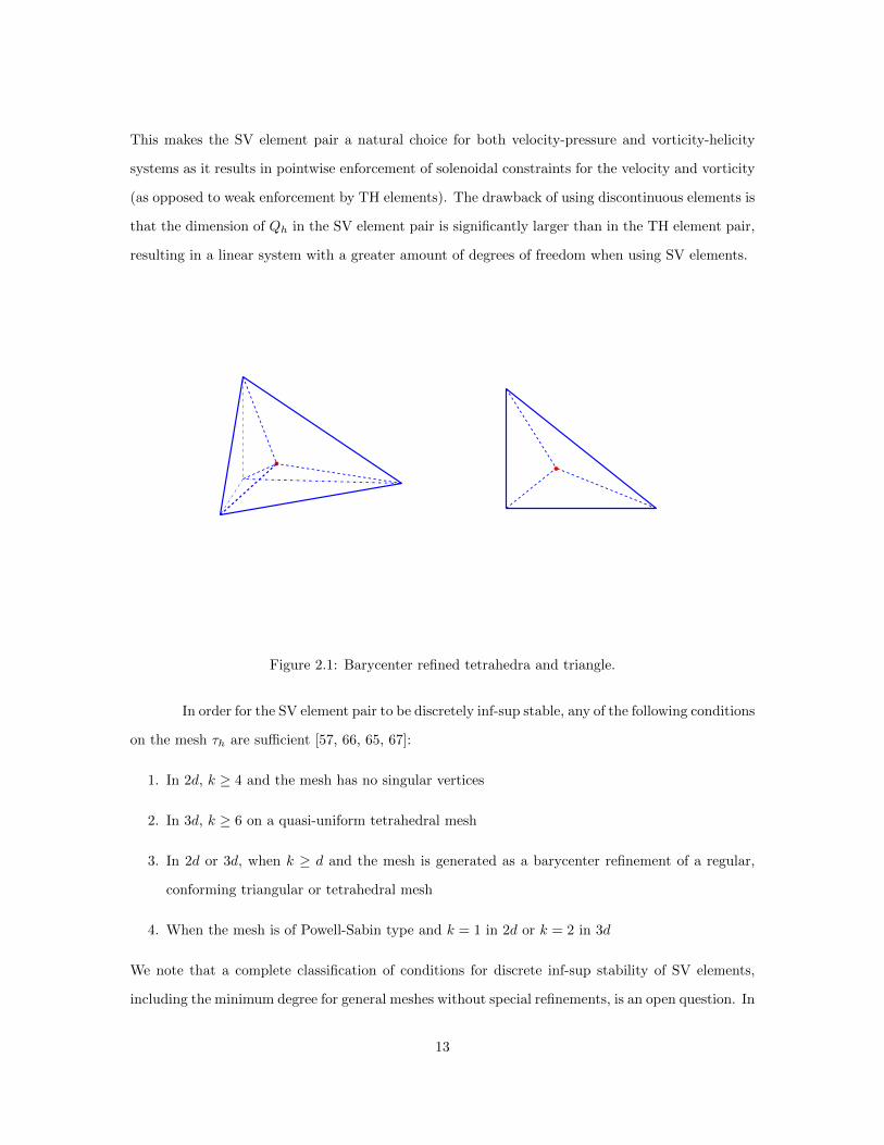
This makes the SV element pair a natural choice for both velocity-pressure and vorticity-helicity
systems as it results in pointwise enforcement of solenoidal constraints for the velocity and vorticity
(as opposed to weak enforcement by TH elements). The drawback of using discontinuous elements is
that the dimension of Qh in the SV element pair is significantly larger than in the TH element pair,
resulting in a linear system with a greater amount of degrees of freedom when using SV elements.
Figure 2.1: Barycenter refined tetrahedra and triangle.
In order for the SV element pair to be discretely inf-sup stable, any of the following conditions
on the mesh τh are sufficient [57, 66, 65, 67]:
1. In 2d, k ≥ 4 and the mesh has no singular vertices
2. In 3d, k ≥ 6 on a quasi-uniform tetrahedral mesh
3. In 2d or 3d, when k ≥ d and the mesh is generated as a barycenter refinement of a regular,
conforming triangular or tetrahedral mesh
4. When the mesh is of Powell-Sabin type and k = 1 in 2d or k = 2 in 3d
We note that a complete classification of conditions for discrete inf-sup stability of SV elements,
including the minimum degree for general meshes without special refinements, is an open question. In
13

our computations performed with SV elements we will always use condition 3. Figure 2.1 illustrates
a barycenter-refined triangle.
For our convergence studies in Chapter 3, 4, and 5 we will assume our choice of finite element
spaces satisfies the following well known approximation properties:
infv∈Xh
‖u− v‖ ≤ Chk+1 ‖u‖k+1 for any u ∈ Hk+1(Ω)
infv∈Xh
‖u− v‖1 ≤ Chk ‖u‖k+1 for any u ∈ Hk+1(Ω)
infr∈Qh
‖p− r‖ ≤ Chs+1 ‖p‖s+1 for any p ∈ Hs+1(Ω).
We note that these approximation properties hold for both TH and SV elements.
In Chapter 5, the trilinear operator b∗ : X×X×X→ R defined by
b∗(u,v,w) := (u · ∇v,w)
will be used. The following useful properties of b∗ are proven in [46].
Lemma 2.0.2. If ∇ · u = 0, then
b∗ (u,v,v) = 0.
Additionally, there exists a constant C dependent on the size of Ω such that
|b∗ (u,v,w) | ≤ C ‖u‖12 ‖∇u‖
12 ‖∇v‖ ‖∇w‖ ,
|b∗ (u,v,w) | ≤ C ‖∇u‖ ‖∇v‖ ‖∇w‖ .
Our error analysis will also use the following discrete version of the Gronwall inequality.
Lemma 2.0.3. Let k,B and aµ, bµ, cµ, γµ, for integers µ ≥ 0, be nonnegative numbers such that
an + k
n∑µ=0
bµ ≤ kn∑µ=0
γµaµ + k
n∑µ=0
cµ +B for n ≥ 0. (2.1)
14
Suppose that kγµ < 1, for all µ, and set σµ = (1− kγµ)−1. Then,
an + k
n∑µ=0
bµ ≤ exp
(k
n∑µ=0
σµγµ
)[k
n∑µ=0
cµ +B
]for n ≥ 0. (2.2)
Remark 2.0.4. If the first sum on the right in (2.1) extends only up to n− 1, then estimate (2.2)
holds for all k > 0, with σµ = 1.
Proof. A proof of these results can be found in [40].
15

Chapter 3
A Numerical Study for a
Velocity-Vorticity-Helicity
formulation of the 3D
Time-Dependent NSE
In this chapter we study a finite element method for the 3d NSE in velocity-vorticity-helicity
form. For Ω ⊂ R3, recent work [56] has shown that the NSE can be equivalently written in VVH
form as: Find u : Ω× (0, T )→ R3 and p : Ω× (0, T )→ R satisfying
∂u
∂t− ν∆u + w × u +∇P = f in Ω× (0, T ), (3.1)
∇ · u = 0 in Ω× (0, T ), (3.2)
u|t=0 = u0 in Ω, (3.3)
u = φ on ∂Ω× (0, T ), (3.4)
16

and find w : Ω× (0, T )→ R3, η : Ω× (0, T )→ R satisfying
∂w
∂t− ν∆w + 2D(w)u−∇η = ∇× f in Ω× (0, T ), (3.5)
∇ ·w = 0 in Ω× (0, T ), (3.6)
w|t=0 = ∇× u0 in Ω, (3.7)
w = ∇× u on ∂Ω× (0, T ), (3.8)
where φ is a Dirichlet boundary condition for velocity satisfying∫
Ωφ · n = 0 ∀t ∈ (0, T ). In [55],
a numerical algorithm based on a 2-step linearization of the VVH formulation was proposed. In
this chapter, we study this discretization of the VVH formulation further by providing a rigorous
stability analysis, testing the method on several benchmark problems, and with various vorticity
boundary conditions.
3.1 Discrete VVH Formulation
For our finite element discretization of the VVH formulation, we will choose velocity and
pressure spaces (Xh, Qh) ⊂ (H10(Ω), L2(Ω)) on our mesh τh to be the Scott-Vogelius element pair
(Pk, Pdisck−1 ). We will denote the vorticity space by Yh, where Yh ⊂ H1(Ω) is the space Pk. We
note that the only difference between the velocity and vorticity finite element spaces is the value of
the finite element functions on the boundary ∂Ω. To simplify the analysis, we require the mesh is
sufficiently regular so that the inverse inequality holds,
‖∇uh‖ ≤ Cih−1 ‖uh‖ . (3.9)
For the initial conditions for our velocity and vorticity approximations we will use the L2 projection
into Vh. For φ ∈ L2(Ω), the L2 projection of φ into Vh, denoted by PVh(φ), satisfies
(PVh(φ),vh) = (φ,vh) for any vh ∈ Vh.
Define the operator A−1h : L2(Ω) → Vh as the solution operator to the discrete Stokes
problem:
(∇A−1h ψ,∇vh) = (ψ,vh), ∀ vh ∈ Vh. (3.10)
17

This operator will not be used in computations, but is used in the analysis of the proposed algorithm.
The following lemma was proven in [50].
Lemma 3.1.1. Assume Ω is such that the Stokes problem is H2-regular. For any ψ ∈ L2(Ω) it
holds
‖A−1h ψ‖L∞ + ‖∇A−1
h ψ‖L3 ≤ C0 ‖ψ‖, (3.11)
and for any f ∈ L2(Ω), q ∈ L2(Ω), and φ ∈ H1(Ω)
|(f ,∇×A−1h ψ)| ≤ C(‖f‖−1 + h‖f‖)‖ψ‖, (3.12)
|(q,∇ ·A−1h ψ)| ≤ C(‖q‖−1 + h‖q‖)‖ψ‖, (3.13)
|(∇φ,∇A−1h ψ)| ≤ C(‖φ‖+ ‖φ‖− 1
2 ,∂Ω + h‖∇φ‖)‖ψ‖. (3.14)
The chosen time discretization is trapezoidal, and the linearization uses second order ex-
trapolation. The fully discrete 2-step version of (3.1)-(3.8) we study is: find (uh,wh, Ph, ηh) ∈
(Xh,Yh, Qh, Qh) satisfying ∀(vh,χh, qh, rh) ∈ (Xh,Xh, Qh, Qh),
Step 1:
1
∆t(un+1h − unh,vh) + ν(∇u
n+ 12
h ,∇vh)− (Pn+1h ,∇ · vh)
+((3
2wnh −
1
2wn−1h )× u
n+ 12
h ,vh)− (fn+ 12 ,vh) = 0, (3.15)
(∇ · un+1h , qh) = 0, (3.16)
Step 2:
1
∆t(wn+1
h −wnh ,χh) + ν(∇w
n+ 12
h ,∇χh)
+(ηn+1h ,∇ · χh) + γν−1((∇×A−1
h wn+ 1
2
h )× un+ 1
2
h , (∇× χh)× un+ 1
2
h ) (3.17)
+2(D(wn+ 1
2
h )un+ 1
2
h ,χh)− (∇× fn+ 12 ,χh) = 0,
(∇ ·wn+1h , rh) = 0, (3.18)
wn+1h |∂Ω − Ih(∇× un+1)|∂Ω = 0, (3.19)
where u0h = PVh
(u0), w0h = PVh
(∇×u0), and Ih denotes an appropriate interpolant. As is common
practice in trapezoidal schemes for fluid flow, the Lagrange multiplier terms are solved for directly
at their n+ 1/2 time levels, i.e. no splitting into time n and n+ 1 pieces is necessary, and so Pn+1h
18

and ηn+1h are approximations to their continuous counterparts at t = tn+1/2. Note also that we have
assumed a homogeneous Dirichlet boundary condition for velocity, and a Dirichlet condition for
vorticity that it be equal to an appropriate interpolant of the curl of the velocity on the boundary.
This is the simplest case for analysis, but is still quite formidable. Extension to other common
boundary conditions will lead to additional technical details, and need to be considered on case by
case basis.
Due to the difficulties associated with any analysis involving the vorticity equation, there are
two components in the above scheme that are for the purposes of analysis only. The unconditional
stability of the velocity does not depend on either of these components of the numerical scheme, but
proving unconditional stability of the vorticity requires both of them.
First, the boundary condition for the discrete vorticity (3.19) is given in terms of the true
velocity, which is not practical. In computations, we use instead the condition
wn+1h |∂Ω − Ih(∇× un+1
h )|∂Ω = 0, (3.20)
however analyzing the system with such a boundary condition does not appear possible in this par-
ticular formulation. Developing improved formulations for which such a vorticity boundary condition
does allow analysis is an important open question. We will consider two possibilities of interpolants
in our computations: i) a nodal interpolant of the L2 projection of the curl of the velocity into Vh,
and ii) a nodal interpolant of a local averaging of the curl of the velocity. A new vorticity boundary
condition, presented in the next section, is also feasible with this discretization.
The second part of the scheme that is not used in computations is the penalty term in
(3.17), i.e. we choose γ = 0 in our computations. In the continuous case this term is consistent
for the homogeneous or periodic boundary conditions on a rectangular box: for sufficiently regular
19

solutions, w = ∇× u, and A−1 the continuous Stokes solution operator, since ∇ · u = 0,
(∇×A−1w)× u = (∇×A−1(∇× u))× u (3.21)
= (A−1(∇× (∇× u)))× u
= (A−1(−∆u−∇(∇ · u))× u
= (A−1(−∆u))× u
= (A−1(Au))× u
= 0.
Outside of the periodic case, the differential operators will not commute and thus errors will arise at
the boundary from this term; hence the term appears to damp vorticity creation at the boundary,
and we do not use it in our computations. However, it does not appear possible to prove a vorticity
stability bound without it.
3.1.1 Stability Analysis
Lemma 3.1.2 (Stability). Assume f ∈ L2(0, T ; H−1(Ω)) and u0 ∈ L2(Ω). Then velocity solutions
to (3.15)-(3.17) are unconditionally stable, and satisfy
∥∥uMh ∥∥2+ ∆t
M−1∑n=0
ν∥∥∥∇u
n+ 12
h
∥∥∥2
≤ ∆t
M−1∑n=0
ν−1∥∥∥fn+ 1
2
∥∥∥2
−1+ C ‖u0‖2 := C4. (3.22)
Proof. Let vh = un+ 1
2
h in (3.15) and simplify to get
1
2∆t(∥∥un+1
h
∥∥2 − ‖unh‖2) + ν
∥∥∥∇un+ 1
2
h
∥∥∥2
= (fn+ 12 ,u
n+ 12
h ).
Using Cauchy Schwarz, Young’s inequality, and simplifying yields
1
2∆t(∥∥un+1
h
∥∥2 − ‖unh‖2) +
ν
2
∥∥∥∇un+ 1
2
h
∥∥∥2
≤ ν−1
2
∥∥∥fn+ 12
∥∥∥2
−1.
20

Multiplying by 2∆t and summing from 0 to M − 1 then gives
∥∥uMh ∥∥2+ ∆t
M−1∑n=0
ν∥∥∥∇u
n+ 12
h
∥∥∥2
≤ ∆t
M−1∑n=0
ν−1∥∥∥fn+ 1
2
∥∥∥2
−1+∥∥u0
h
∥∥2
≤ ∆t
M−1∑n=0
ν−1∥∥∥fn+ 1
2
∥∥∥2
−1+ C ‖u0‖2 ,
which proves the estimate (3.22).
Remark 3.1.3. We note that the unconditional stability of the velocity solution is independent of
both the vorticity boundary condition and the penalty term of the discrete vorticity equation.
Lemma 3.1.4. Assume f ∈ L2(0, T ; L2(Ω)), u0 ∈ H10(Ω), u ∈ L∞(0, T ; H2(Ω)),
ut ∈ L∞(0, T ; H1(Ω)), and utt ∈ L∞(0, T ; H1(Ω)). Then vorticity solutions are also stable, in the
sense of ∥∥∇A−1h wM
h
∥∥2+ ∆t
M−1∑n=0
ν∥∥∥wn+ 1
2
h
∥∥∥2
≤ C(ν−2, C4,M, T, f ,u) := C5. (3.23)
Remark 3.1.5. It appears that the penalty parameter γ needs to satisfy γ > 12 for the proof to
hold. When γ = 0, we are reduced to the non-penalty term case, for which we are unable to prove
unconditional stability.
Proof. For the vorticity bound, let wnh∗ = Ih(∇ × un) where Ih is a discretely div-free preserving
interpolant. Note wnh∗ ∈ Vh and wn
h∗ satisfies the vorticity boundary condition (3.19). The vorticity
solution can then be decomposed as
wn+ 1
2
h = wn+ 1
2
h
∗+ w
n+ 12
h , (3.24)
where wn+ 1
2
h ∈ Vh. Letting Ih(∇× u) ≤ Cu for all t, we have
∥∥∥∥wn+ 12
h
∗∥∥∥∥ ≤ Cu. (3.25)
21

Substituting (3.24) into the vorticity equation (3.17) yields, ∀χh ∈ Vh,
1
∆t(wn+1
h −wnh ,χh) + γν−1((∇×A−1
h wn+ 1
2
h )× un+ 1
2
h , (∇× χh)× un+ 1
2
h )
+ ν(∇wn+ 1
2
h ,∇χh) = (∇× fn+ 12 ,χh)− 2(D(w
n+ 12
h )un+ 1
2
h ,χh)
− γν−1((∇×A−1h w
n+ 12
h
∗)× u
n+ 12
h , (∇× χh)× un+ 1
2
h )
− 2(D(wn+ 1
2
h
∗)un+ 1
2
h ,χh)− ν(∇wn+ 1
2
h
∗,∇χh)− 1
∆t(wn+1
h
∗ −wnh∗,χh). (3.26)
Let χh = A−1h w
n+ 12
h and simplify to get
1
∆t(wn+1
h −wnh , A
−1h w
n+ 12
h ) + γν−1
∥∥∥∥(∇×A−1h w
n+ 12
h )× un+ 1
2
h
∥∥∥∥2
+ ν
∥∥∥∥wn+ 12
h
∥∥∥∥2
= (∇× fn+ 12 , A−1
h wn+ 1
2
h )− 2(D(wn+ 1
2
h )un+ 1
2
h , A−1h w
n+ 12
h )
− 2(D(wn+ 1
2
h
∗)un+ 1
2
h , A−1h w
n+ 12
h )− ν(∇wn+ 1
2
h
∗,∇A−1
h wn+ 1
2
h )
− γν−1((∇×A−1h w
n+ 12
h
∗)× u
n+ 12
h , (∇×A−1h w
n+ 12
h )× un+ 1
2
h )
− 1
∆t(wn+1
h
∗ −wnh∗, A−1
h wn+ 1
2
h ). (3.27)
It is straightforward to show that A−1h is a symmetric operator on Vh and thus
1
∆t(wn+1
h −wnh , A
−1h w
n+ 12
h ) =1
2∆t[(wn+1
h , A−1h wn+1
h ) + (wn+1h , A−1
h wnh)
−(wnh , A
−1h wn+1
h )− (wnh , A
−1h wn
h)]
=1
2∆t[(wn+1
h , A−1h wn+1
h )− (wnh , A
−1h wn
h)]
=1
2∆t(∥∥∥∇A−1
h wn+1h
∥∥∥2
−∥∥∇A−1
h wnh
∥∥2). (3.28)
Using (3.12) on the first RHS term of (3.27) yields
(∇× fn+ 12 , A−1
h wn+ 1
2
h ) = (fn+ 12 ,∇×A−1
h wn+ 1
2
h )
≤ C(∥∥∥fn+ 1
2
∥∥∥V ∗
+ h∥∥∥fn+ 1
2
∥∥∥)
∥∥∥∥wn+ 12
h
∥∥∥∥ (3.29)
≤ C(ε)ν−1(∥∥∥fn+ 1
2
∥∥∥2
V ∗+ h2
∥∥∥fn+ 12
∥∥∥2
) + νε
∥∥∥∥wn+ 12
h
∥∥∥∥2
.
Using vector identities, integration by parts, and that A−1h w
n+ 12
h is divergence free, on the first
22

trilinear term in (3.27) gives
|2(D(wn+ 1
2
h )un+ 1
2
h , A−1h w
n+ 12
h )|
= |(∇× (wn+ 1
2
h × un+ 1
2
h )−∇(un+ 1
2
h ·wn+ 12
h ), A−1h w
n+ 12
h )|
= |(∇× (wn+ 1
2
h × un+ 1
2
h ), A−1h w
n+ 12
h )|+ |(un+ 12
h ·wn+ 12
h ,∇ ·A−1h w
n+ 12
h )|
= |(wn+ 12
h × un+ 1
2
h ,∇×A−1h w
n+ 12
h )|
= |(wn+ 12
h , (∇×A−1h w
n+ 12
h )× un+ 1
2
h )| (3.30)
≤ γ−1ν
2
∥∥∥∥wn+ 12
h
∥∥∥∥2
+γν−1
2
∥∥∥∥(∇×A−1h w
n+ 12
h )× un+ 1
2
h
∥∥∥∥2
.
The part of the penalty term on the right-hand side of (3.27) is majorized as
−γν−1((∇×A−1h w
n+ 12
h
∗)× u
n+ 12
h , (∇×A−1h w
n+ 12
h )× un+ 1
2
h ) (3.31)
≤ γν−1
∥∥∥∥(∇×A−1h w
n+ 12
h
∗)× u
n+ 12
h
∥∥∥∥∥∥∥∥(∇×A−1h w
n+ 12
h )× un+ 1
2
h
∥∥∥∥≤ γν−1
∥∥∥∥(∇×A−1h w
n+ 12
h
∗)× u
n+ 12
h
∥∥∥∥2
+γν−1
4
∥∥∥∥(∇×A−1h w
n+ 12
h )× un+ 1
2
h
∥∥∥∥2
.
The first term on the right hand side of (3.31) can be bounded using Holder’s inequality, (3.25) and
Lemma 3.1.1:
∥∥∥∥(∇×A−1h w
n+ 12
h
∗)× u
n+ 12
h
∥∥∥∥2
≤ C
∥∥∥∥∇×A−1h w
n+ 12
h
∗∥∥∥∥2
L3
∥∥∥un+ 12
h
∥∥∥2
L6
≤ CC20
∥∥∥∥wn+ 12
h
∗∥∥∥∥2 ∥∥∥∇u
n+ 12
h
∥∥∥2
(3.32)
≤ CC20C
2u
∥∥∥∇un+ 1
2
h
∥∥∥2
. (3.33)
Substituting back into (3.31) we now have
−γν−1((∇×A−1h w
n+ 12
h
∗)× u
n+ 12
h , (∇×A−1h w
n+ 12
h )× un+ 1
2
h )
≤ γν−1CC20C
2u
∥∥∥∇un+ 1
2
h
∥∥∥2
+γν−1
4
∥∥∥∥(∇×A−1h w
n+ 12
h )× un+ 1
2
h
∥∥∥∥2
. (3.34)
23

The second trilinear term in (3.27) can be bounded using Lemma 3.1.1 and 3.1.2 to obtain
2(D(wn+ 1
2
h
∗)un+ 1
2
h , A−1h w
n+ 12
h ) ≤ C
∥∥∥∥∇wn+ 1
2
h
∗∥∥∥∥ ∥∥∥un+ 1
2
h
∥∥∥∥∥∥∥A−1h w
n+ 12
h
∥∥∥∥L∞
≤ C(ε)C4ν−1
∥∥∥∥∇wn+ 1
2
h
∗∥∥∥∥2
+ νε
∥∥∥∥wn+ 12
h
∥∥∥∥2
(3.35)
≤ C(ε)C4C2uν−1 + νε
∥∥∥∥wn+ 12
h
∥∥∥∥2
. (3.36)
Using (3.14) gives
ν(∇wn+ 1
2
h
∗,∇A−1
h wn+ 1
2
h ) ≤ Cν(
∥∥∥∥wn+ 12
h
∗∥∥∥∥+
∥∥∥∥wn+ 12
h
∗∥∥∥∥− 1
2 ,∂Ω
+ h
∥∥∥∥∇wn+ 1
2
h
∗∥∥∥∥)
∥∥∥∥wn+ 12
h
∥∥∥∥≤ C(ε)ν(
∥∥∥∥wn+ 12
h
∗∥∥∥∥2
+
∥∥∥∥wn+ 12
h
∗∥∥∥∥2
− 12 ,∂Ω
+ h2
∥∥∥∥∇wn+ 1
2
h
∗∥∥∥∥2
)
+νε
∥∥∥∥wn+ 12
h
∥∥∥∥2
≤ C(ε)C2uν + νε
∥∥∥∥wn+ 12
h
∥∥∥∥2
. (3.37)
Finally, Cauchy Schwarz, Young’s inequality, and the definition of wnh∗ yield
1
∆t(wn+1
h
∗ −wnh∗, A−1
h wn+ 1
2
h ) ≤∥∥∥∥Ih(∇× (
un+1 − un
∆t))
∥∥∥∥∥∥∥∥A−1h w
n+ 12
h
∥∥∥∥≤ C0
∥∥Ih(∇× (ut(tn+1) + utt(t
∗)))∥∥∥∥∥∥wn+ 1
2
h
∥∥∥∥ (3.38)
≤ C0C(ε)ν−1(∥∥Ih(∇× ut(t
n+1))∥∥2
+ ‖Ih(∇× utt(t∗))‖2)
+νε
∥∥∥∥wn+ 12
h
∥∥∥∥2
≤ C0C(ε)ν−1 + νε
∥∥∥∥wn+ 12
h
∥∥∥∥2
.
Substitute into (3.27) using (3.28)-(3.38) to get
1
2∆t
(∥∥∥∇A−1h wn+1
h
∥∥∥2
−∥∥∇A−1
h wnh
∥∥2)
+ ν
(1− 1
2γ− 4ε
)∥∥∥∥wn+ 12
h
∥∥∥∥2
≤ Cν−1
(∥∥∥fn+ 12
∥∥∥2
V ∗+ h2
∥∥∥fn+ 12
∥∥∥2)
+ γν−1CC0C2u
∥∥∥∇un+ 1
2
h
∥∥∥2
+ C(ε)C4ν−1C2
u + C(ε)νC2u + C0C(ε)ν−1. (3.39)
24

Choosing an arbitrarily small ε, the penalty parameter γ satisfying (1 − 12γ − 4ε) > 0, multiplying
by 2∆t, and summing from 0 to M − 1 yield
∥∥∥∇A−1h wM
h
∥∥∥2
+ ∆t
M−1∑n=0
1
4ν
∥∥∥∥wn+ 12
h
∥∥∥∥2
≤ ν−1∆tC
M−1∑n=0
(∥∥∥fn+ 1
2
∥∥∥2
V ∗+ h2
∥∥∥fn+ 12
∥∥∥2
)
+ C(ν−1, C4, Cu, ν) +∥∥∥∇A−1
h w0h
∥∥∥2
+ γν−2CC0C2u∆t
M−1∑n=0
ν∥∥∥∇u
n+ 12
h
∥∥∥2
. (3.40)
Using the result for the velocity stability bound on the last sum of (3.40) finishes the proof.
3.2 Numerical Results
We now present two numerical experiments to test the VVH method studied in this chapter.
For all tests, we use (P3, Pdisc2 ) Scott-Vogelius elements, on barycenter-refined tetrahedral meshes.
To solve the linear systems, we use the robust and efficient method proposed in [56] for this element
choice. This is the lowest order element pair that is LBB stable on this mesh. The first experiment
confirms expected convergence rates, and the second tests the method on 3D channel flow over a
step.
All computations use γ = 0. In the computations, vorticity appears to be stable with this
choice, and so it was not necessary to add this (costly) stabilization term. However, proving discrete
stability of vorticity does not seem possible in this case, and so its use is believed to cover a gap in
the analysis only.
3.2.1 Convergence Rates
Our first experiment is used to test convergence rates for the problem Ω = (0, 1)3, where
the true solution is given by
u(x, y, z, t) =
(1 + .01t) cos(2πz)
(1 + .01t) sin(2πz)
(1 + .01t) sin(2πx)
(3.41)
For this problem we take ν = 1, and initial condition u0h = PVh
(u0),w0h = PVh
(∇×u0). We compute
with end time T = 1, and monitor error while decreasing the values of ∆t with h. Uniform meshes
25

are used in the sense that each mesh divides Ω into equal size cubes, then divides each cube into six
tetrahedra, and then performs a barycenter refinement of each tetrahedra. In the tables, h denotes
the length of a side of a cube. For the velocity boundary condition, we use the nodal interpolant of
the true solution on the boundary. For the vorticity boundary condition, we compute three different
ways, all using a Dirichlet condition for discrete vorticity: using the nodal interpolant of the true
vorticity, using the nodal interpolant of the L2 projection of the curl of the discrete velocity into
Vh, and also using a simple local averaging of the curl of the discrete velocity.
The results are shown in Tables 3.1-3.3, respectively. With our choice of elements and a
trapezoidal time discretization, optimal error is O(∆t2 + h3), and since we tie together the spatial
and temporal refinements by cutting ∆t in third when h is cut in half, O(h3) is optimal. All
three vorticity boundary conditions provide similar results: suboptimal rates are observed in the
L2(0, T ; H1(Ω)) norm until the last mesh refinement, when the rate jumps to around 3. We also
see that for the velocity in the L2(0, T ; L2(Ω)) norm we see optimal convergence rates, where as the
vorticity in the L2(0, T ; L2(Ω)) norm we do not seem to recover any L2 lift. Here, while the errors
observed using the (more practical) non-exact boundary conditions are expectably larger, the rates
of convergence observed do not seem to decrease. A complete convergence theory for the method
currently appears impenetrable without several assumptions not needed for usual NSE analysis, but
progress on this front will likely lead to answers about boundary-dependence of convergence rates.
h dof ∆t ‖u− uh‖L2(0,T ;L2(Ω)) Rate ‖u− uh‖L2(0,T ;H1(Ω)) Rate
1/2 10,218 1 3.8609e-2 - 8.6168e-2 -1/4 78,462 1/3 2.3317e-3 4.0495 9.5332e-3 3.17611/6 261,474 1/6 4.6873e-4 3.9568 2.7359e-3 3.07871/8 615,990 1/9 1.5074e-4 3.9435 1.1360e-3 3.05331/10 1,198,746 1/18 5.9864e-5 4.1385 5.4716e-4 3.2738
h ∆t ‖w −wh‖L2(0,T ;L2(Ω)) Rate ‖w −wh‖L2(0,T ;H1(Ω)) Rate
1/2 1 4.4557e-1 - 2.1412 -1/4 1/3 4.6819e-2 3.2505 4.4218e-1 2.27571/6 1/6 1.2533e-2 3.2504 1.7694e-1 2.25891/8 1/9 5.0199e-3 3.1804 9.4030e-2 2.19761/10 1/18 2.4978e-3 3.1280 4.8454e-2 2.9712
Table 3.1: Velocity and Vorticity errors and convergence rates using the nodal interpolant of thetrue vorticity for the vorticity boundary condition.
26

h ∆t ‖u− uh‖L2(0,T ;L2(Ω)) Rate ‖u− uh‖L2(0,T ;H1(Ω)) Rate
1/2 1/1 3.8609e-2 - 8.6168e-2 -1/4 1/3 2.3317e-3 4.0495 9.5343e-3 3.17601/6 1/6 4.6873e-4 3.9568 2.7361e-3 3.07881/8 1/9 1.5074e-4 3.9435 1.1361e-3 3.05521/10 1/18 5.9864e-5 4.1385 5.4719e-4 3.2739
h ∆t ‖w −wh‖L2(0,T ;L2(Ω)) Rate ‖w −wh‖L2(0,T ;H1(Ω)) Rate
1/2 1/1 7.0753e-1 - 2.7086 -1/4 1/3 7.3843e-2 3.2603 5.1060e-1 2.40731/6 1/6 1.9136e-2 3.3304 1.9562e-1 2.36621/8 1/9 7.4270e-3 3.2899 1.0169e-1 2.27421/10 1/18 3.4219e-3 3.4728 5.2398e-2 2.9715
Table 3.2: Velocity and Vorticity errors and convergence rates using the nodal interpolant of the L2
projection of the curl of the discrete velocity into Vh, for the vorticity boundary condition.
h ∆t ‖u− uh‖L2(0,T ;L2(Ω)) Rate ‖u− uh‖L2(0,T ;H1(Ω)) Rate
1/2 1/1 3.8609e-2 - 8.6168e-2 -1/4 1/3 2.3317e-3 4.0495 9.5342e-3 3.17601/6 1/6 4.6873e-4 3.9568 2.7361e-3 3.07881/8 1/9 1.5074e-4 3.9435 1.1361e-3 3.05521/10 1/18 5.9864e-5 4.1385 5.4720e-4 3.2739
h ∆t ‖w −wh‖L2(0,T ;L2(Ω)) Rate ‖w −wh‖L2(0,T ;H1(Ω)) Rate
1/2 1/1 6.6951e-1 - 2.6394 -1/4 1/3 8.0245e-2 3.0606 5.0373e-1 2.38951/6 1/6 2.0989e-2 3.3075 1.9434e-1 2.34901/8 1/9 8.2120e-3 3.2619 1.0115e-1 2.26991/10 1/18 3.8818e-3 3.3579 5.2427e-2 2.9451
Table 3.3: Velocity and Vorticity errors and convergence rates using nodal averages of the curl ofthe discrete velocity for the vorticity boundary condition.
27
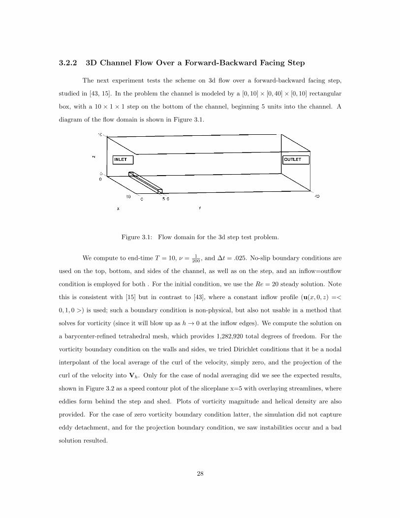
3.2.2 3D Channel Flow Over a Forward-Backward Facing Step
The next experiment tests the scheme on 3d flow over a forward-backward facing step,
studied in [43, 15]. In the problem the channel is modeled by a [0, 10]× [0, 40]× [0, 10] rectangular
box, with a 10 × 1 × 1 step on the bottom of the channel, beginning 5 units into the channel. A
diagram of the flow domain is shown in Figure 3.1.
Figure 3.1: Flow domain for the 3d step test problem.
We compute to end-time T = 10, ν = 1200 , and ∆t = .025. No-slip boundary conditions are
used on the top, bottom, and sides of the channel, as well as on the step, and an inflow=outflow
condition is employed for both . For the initial condition, we use the Re = 20 steady solution. Note
this is consistent with [15] but in contrast to [43], where a constant inflow profile (u(x, 0, z) =<
0, 1, 0 >) is used; such a boundary condition is non-physical, but also not usable in a method that
solves for vorticity (since it will blow up as h→ 0 at the inflow edges). We compute the solution on
a barycenter-refined tetrahedral mesh, which provides 1,282,920 total degrees of freedom. For the
vorticity boundary condition on the walls and sides, we tried Dirichlet conditions that it be a nodal
interpolant of the local average of the curl of the velocity, simply zero, and the projection of the
curl of the velocity into Vh. Only for the case of nodal averaging did we see the expected results,
shown in Figure 3.2 as a speed contour plot of the sliceplane x=5 with overlaying streamlines, where
eddies form behind the step and shed. Plots of vorticity magnitude and helical density are also
provided. For the case of zero vorticity boundary condition latter, the simulation did not capture
eddy detachment, and for the projection boundary condition, we saw instabilities occur and a bad
solution resulted.
28
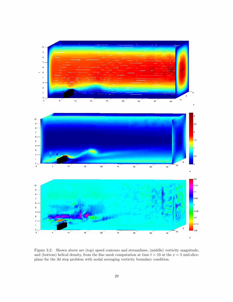
Figure 3.2: Shown above are (top) speed contours and streamlines, (middle) vorticity magnitude,and (bottom) helical density, from the fine mesh computation at time t = 10 at the x = 5 mid-slice-plane for the 3d step problem with nodal averaging vorticity boundary condition.
29

Chapter 4
Natural vorticity boundary
conditions for coupled vorticity
equations
This chapter derives new natural boundary conditions for the vorticity equations that result
from the application of the curl operator to the steady NSE momentum equation, given by
−ν∆w + (u · ∇)w − (w · ∇)u = ∇× f . (4.1)
A finite element method for solving the 3d vorticity equations is presented to test the accuracy of
the proposed boundary conditions, and results from a simple numerical experiment are presented
verifying optimal convergence rates are acheived. We note that the vorticity boundary conditions
presented herein could also easily be derived for the time-dependent vorticity equations, and would
apply equally well to the vorticity-helical density equations studied in the previous chapter.
4.1 Derivation
Suppose we are given some general Dirichlet boundary condition for the velocity in the NSE,
i.e. u = g on ∂Ω. We are mainly interested in the case where ∂Ω is a solid wall with no-slip (g = 0)
30

boundary conditions, and so leaving g to be general includes this case. Our first vorticity boundary
condition easily follows:
w · n = (∇× g) · n on ∂Ω. (4.2)
To deduce two more boundary conditions for w, consider the incompressible NSE written in rota-
tional form (see, e.g. [32] for more on rotational form of NSE),
ν∇×w + w × u +∇P = f ,
where P = 12 |u|
2 + p is the Bernoulli pressure. Taking the tangential component of both sides of
this equation gives
ν(∇×w)× n = (f −∇P −w × g)× n on ∂Ω, (4.3)
which provides two more boundary conditions for w in terms of the primitive NSE velocity and
pressure variables. In velocity-vorticity splitting schemes where the NSE momentum equation is
used for the velocity (as in the work of Wong and Baker [62] or the scheme presented in the previous
chapter of this work), the NSE velocity and pressure are considered as knowns when solving the
vorticity (or vorticity-helical density) equations.
We observe that the boundary condition (4.3) is the natural boundary condition for the
following weak formulation of the vorticity equation: Find w ∈ H0(div) ∩H(curl) satisfying
ν(∇×w,∇× v) + ν(∇ ·w,∇ · v) + ((u · ∇)w − (w · ∇)u,v)
+
∮∂Ω
((w × g)× n) · v ds = (∇× f ,v) +
∮∂Ω
((f −∇P )× n) · v ds, (4.4)
for any v ∈ H0(div) ∩H(curl).
To avoid computing pressure gradient over ∂Ω we rewrite the last term in (4.4) using inte-
gration by parts on ∂Ω. To this end, we use the surface gradient and divergence, defined as:
∇Γp = ∇p− (n · ∇p)n, and divΓv = tr(∇Γv),
which are intrinsic surface quantities and do not depend on an extension of a scalar function p and
a vector quantity v off a surface. We also need the following identity, proved in [34], for a smooth,
31

closed surface Γ: ∫Γ
p divΓv + v · ∇Γp ds =
∫Γ
κ(v · n)p ds, (4.5)
where κ is the surface mean curvature.
From the definition of the surface gradient we immediately get the identity:
(∇P )× n = (∇ΓP )× n.
Hence, with (4.5) we see
∮∂Ω
((∇P )× n) · v ds =
∮∂Ω
((∇ΓP )× n) · v ds =
∮∂Ω
(v × n) · ∇ΓP ds
= −∮∂Ω
PdivΓ(v × n) ds. (4.6)
Finally, using v · n = 0 we have
divΓ(v × n) = (∇× v) · n.
Thus, the weak formulation of the vorticity equation now reads: Find w ∈ H0(div) ∩ H(curl)
satisfying
ν(∇×w,∇× v) + ν(∇ ·w,∇ · v) + ((u · ∇)w − (w · ∇)u,v)
+
∮∂Ω
((w × g)× n) · v ds = (∇× f ,v) +
∮∂Ω
(f × n) · v ds +
∮∂Ω
P (∇× v) · n ds, (4.7)
for any v ∈ H0(div) ∩ H(curl). In the case of no slip boundary conditions (g = 0), the system
reduces to
ν(∇×w,∇× v) + ν(∇ ·w,∇ · v) + ((u · ∇)w − (w · ∇)u,v)
= (∇× f ,v) +
∮∂Ω
(f × n) · v ds +
∮∂Ω
p(∇× v) · n ds. (4.8)
4.2 Numerical Results
In this section we consider a basic 3d numerical test designed to evaluate the accuracy
of a numerical scheme implementing our new vorticity boundary conditions. Let I denote some
32

interpolation operator on ∂Ω. The scheme we propose to compute with is given in two steps:
Step 1:
ν(∇uh,∇vh) + (uh · ∇uh,vh)− (ph,∇ · vh) = (f ,vh)
(∇ · uh, qh) = 0
uh|∂Ω = I(g)
Step 2:
ν(∇×wh,∇× vh) + ν(∇ ·wh,∇ · vh) + ((uh · ∇)wh − (wh · ∇)uh,vh) +
∫∂Ω
((wh × g)× n) · vh ds
= (∇× f ,vh) +
∫∂Ω
(f × n) · vh ds +
∫∂Ω
p(∇× vh) · n ds
(wh − I(∇× g)) · n|∂Ω = 0.
Our 3d numerical experiment is designed to test convergence rates for the problem Ω =
(0, 1)3, where the true, steady NSE solution is given by
u1(x, y, z) = sin(2πy)
u2(x, y, z) = cos(2πz)
u3(x, y, z) = ex
p(x, y, z) = sin(2πx) + cos(2πy) + sin(2πz),
where p denotes the standard NSE pressure. Because we are given nonhomogenous boundary con-
ditions for the velocity, if we want to enforce vorticity boundary conditions only with boundary
integrals, we must include the left hand side term
∫∂Ω
((wh×g)×n) ·vh ds in the vorticity equation.
We compute with Reynolds number Re = 1 and force field
f = u · ∇u +∇p− ν∆u
as determined by the true NSE solution. Velocity and vorticity approximations are computed using
Q2 elements, while Q1 elements are used for the pressure. All computations were performed using
the software deal.II [6, 7].
33
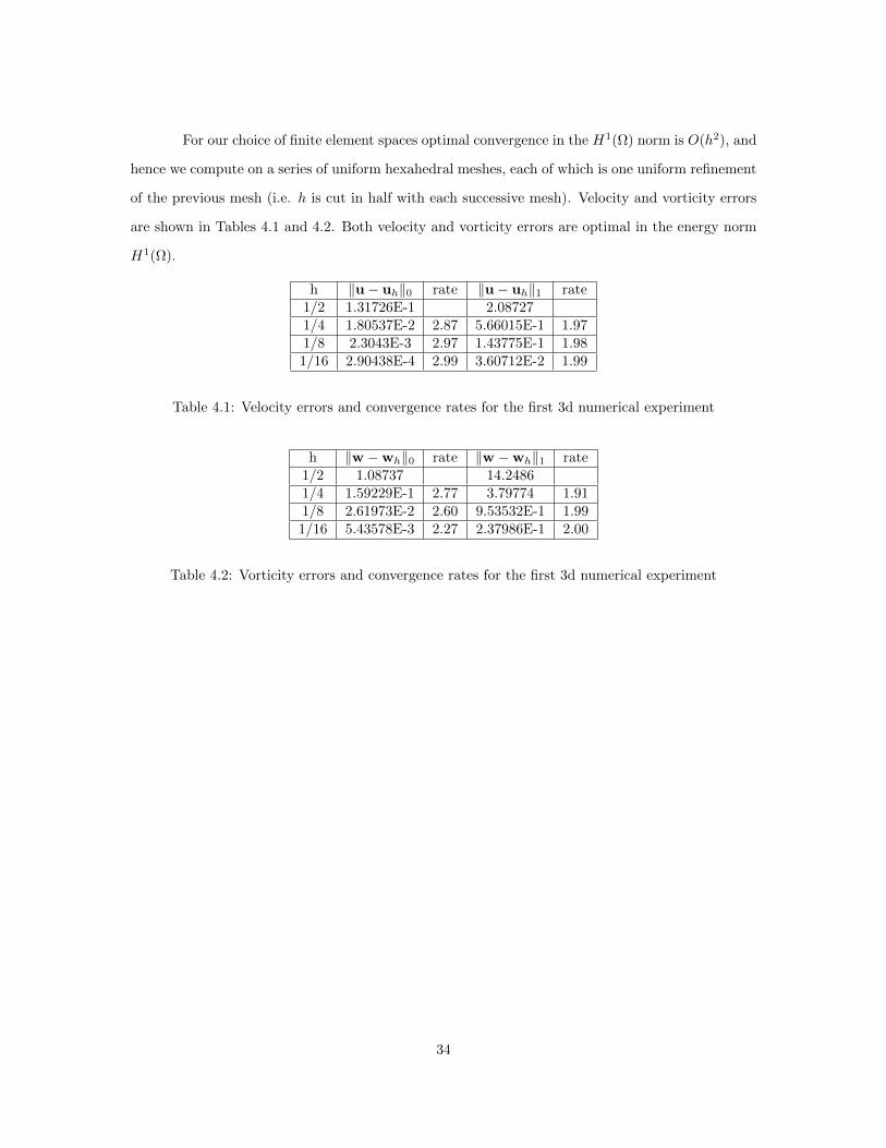
For our choice of finite element spaces optimal convergence in the H1(Ω) norm is O(h2), and
hence we compute on a series of uniform hexahedral meshes, each of which is one uniform refinement
of the previous mesh (i.e. h is cut in half with each successive mesh). Velocity and vorticity errors
are shown in Tables 4.1 and 4.2. Both velocity and vorticity errors are optimal in the energy norm
H1(Ω).
h ‖u− uh‖0 rate ‖u− uh‖1 rate1/2 1.31726E-1 2.087271/4 1.80537E-2 2.87 5.66015E-1 1.971/8 2.3043E-3 2.97 1.43775E-1 1.981/16 2.90438E-4 2.99 3.60712E-2 1.99
Table 4.1: Velocity errors and convergence rates for the first 3d numerical experiment
h ‖w −wh‖0 rate ‖w −wh‖1 rate1/2 1.08737 14.24861/4 1.59229E-1 2.77 3.79774 1.911/8 2.61973E-2 2.60 9.53532E-1 1.991/16 5.43578E-3 2.27 2.37986E-1 2.00
Table 4.2: Vorticity errors and convergence rates for the first 3d numerical experiment
34

Chapter 5
A New Reduced Order Multiscale
Deconvolution Model
This chapter proposes a new reduced order multiscale deconvolution model (MDM). This
model leads to a natural, efficient numerical scheme that is both unconditionally stable and optimally
accurate. Numerical tests are provided that confirm the effectiveness of the scheme.
5.1 Derivation
Recall the NSE, given by
ut + u · ∇u +∇p− ν∆u = f (5.1)
∇ · u = 0. (5.2)
In this chapter we will only consider homogenous Dirichlet boundary conditions for the velocity u.
Our model formulation will use two different incompressible Helmholtz filters, the first of which is
35
defined by
−α2∆u + α2∇λ+ u = u, (5.3)
∇ · u = 0, (5.4)
(u− u)|∂Ω = 0, (5.5)
where α denotes the length scale associated with the filtered velocity u. For convenience, we will
denote the solution operator to (5.3)-(5.5) by Fα(·), i.e. Fαu = u. The second incompressible
Helmholtz filter is given by
−γ2∆u + γ2∇ρ+ u = u, (5.6)
∇ · u = 0, (5.7)
(u− u)|∂Ω = 0, (5.8)
where γ is a second, intermediate length scale associated with the filtered velocity u, satisfying
0 < γ ≤ α. In practice, α is generally chosen to be the size of the smallest flow structures to be
resolved, and γ is a parameter determining the modeling error relative to the NSE. In [22] it was
shown that u has an explicit form depending on u given by
u =α2
γ2u− (1− α2
γ2)u,
so we will define our multiscale, approximate deconvolution operator Gγ as
Gγu :=α2
γ2u + (1− α2
γ2)u =
α2
γ2u− α2 − γ2
γ2u. (5.9)
Using this definition we immediately see that we can write the intermediate filtered quantity φ
explicitly as
u ≈ u = Gγu.
36

Because Fα is invertible we can write u = Fα−1u, and using the definition of the α-filter (5.3) on
the time derivative term, the NSE momentum equation (1.1) becomes
(−α2∆ut + α2∇λt + ut) + Fα−1u · ∇(Fα
−1u) +∇p− ν∆(Fα−1u) = f . (5.10)
It was shown in [22] that we have the following local error estimate for the accuracy in approximating
the operator Fα−1 by Gγ :
‖u−Gγu‖Hk(Ω) = ‖u− u‖Hk(Ω) ≤ γ2 ‖u‖Hk+2(Ω) .
This estimate suggests that multiscale, approximate deconvolution can be used to approximate the
inverse of the α-filter (i.e. Fα−1φ ≈ Gγφ). Thus, denoting v := u and q := p + α2λt in (5.10), we
arrive at
vt − α2∆vt +Gγv · ∇Gγv +∇q − ν∆Gγv = f .
Employing the same multiscale, approximate deconvolution approximation in the conservation of
mass equation (5.2) yields ∇ · Gγu = ∇ · Gγv = 0. Note that by (5.7) and the definition of
the deconvolution operator Gγ , the new conservation of mass constraint is satisfied via enforcing
∇ · v = 0. The reduced order multiscale deconvolution model (RMDM) with incompressible filters
for homogenous Dirichlet boundary conditions is then
vt − α2∆vt +Gγv · ∇Gγv +∇q − ν∆Gγv = f (5.11)
∇ · v = 0 (5.12)
−γ2∆v + γ2∇ρ+ v = v (5.13)
∇ · v = 0 (5.14)
(v − v)|∂Ω = 0. (5.15)
5.2 The Discrete Setting
Define finite dimensional spaces Xh ⊂ X and Qh ⊂ Q to be the Scott-Vogelius (SV) mixed
finite element pair (Xh, Qh) := (Pk(τh), P disck−1 (τh)).
The following discrete filter is defined analogously to its continuous counterpart by taking
37

its variational formulation and restricting to finite dimensional spaces.
Definition 5.2.1. Given φ ∈ L2(Ω), define φh
to be the solution of the problem: Find (φh, ρh) ∈
(Xh, Qh) satisfying
γ2(∇φh,∇χh) + (φ
h,χh)− (ρh,∇ · χh) = (φ,χh)∀χh ∈ Xh, (5.16)
(∇ · φh, qh) = 0∀ qh ∈ Qh. (5.17)
We will denote the solution operator of this discrete filter by Fh, i.e. Fhφ := φh. The
equivalent discretely divergence-free representation of the filter is: Given φ ∈ L2(Ω), find φh∈ Vh
satisfying
γ2(∇φh,∇χh) + (φ
h,χh) = (φ,χh)∀χh ∈ Vh.
The following lemma, found in [58], contains useful bounds for discretely filtered functions.
Lemma 5.2.2. For φ ∈ L2(Ω), ∥∥∥φh∥∥∥ ≤ ‖φ‖ .For φ ∈ X, there exists a constant C dependent on the size of Ω such that
∥∥∥∇φh∥∥∥ ≤ C ‖∇φ‖ .For φ ∈ Vh, ∥∥∥∇φh∥∥∥ ≤ ‖∇φ‖ .
The next lemma provides a bound on the difference between continuously filtered and dis-
cretely filtered functions.
Lemma 5.2.3. For φ ∈ Hk(Ω) ∩V we have the bound
∥∥∥φ− φh∥∥∥2
+ γ2∥∥∥∇(φ− φ
h)∥∥∥2
≤ C(γ−2h2k+2 + h2k)|φ|2k+1. (5.18)
For k ≤ 2, we have the improved bound
∥∥∥φ− φh∥∥∥2
+ γ2∥∥∥∇(φ− φ
h)∥∥∥2
≤ C(h2k+2 + γ2h2k)|φ|2k+1. (5.19)
38
Proof. Multiplying the γ-filter equation (5.6) by arbitrary χh ∈ Vh and integrating over Ω yields
γ2(∇φ,∇χh) + (φ,χh) = (φ,χh).
Subtracting the discrete γ-filter equation (5.16) and denoting e = φ− φh
gives, for any χh ∈ Vh,
γ2(∇e,∇χh) + (e,χh) = 0.
Standard finite element analysis and interpolation estimates produce the bound
∥∥∥φ− φh∥∥∥2
+ γ2∥∥∥∇(φ− φ
h)∥∥∥2
≤ C(h2k+2 + γ2h2k)|φ|2k+1.
In [47] it was shown that for k ≥ 3 we have the estimate γ2|φ|2k+1 ≤ C|φ|2k+1, and hence we get the
bound
∥∥∥φ− φh∥∥∥2
+ γ2∥∥∥∇(φ− φ
h)∥∥∥2
≤ C(γ−2h2k+2 + h2k)|φ|2k+1.
Additionally, for k = 0, 1, 2 it was shown in [47] that we have the improved estimate |φ|k ≤ |φ|k,
which finishes the proof.
5.2.1 An Unconditionally Stable Algorithm for the RMDM
The fully discrete algorithm we study for the RMDM is backward Euler in time and finite
element in space.
Algorithm 5.2.4. Given two filtering radii α ≥ γ > 0, initial velocity v0h ∈ Vh, a forcing function
f ∈ L∞(0, T ; H−1(Ω)), end time T > 0, and timestep ∆t > 0, set M = T∆t and compute for
n = 1, 2, ...,M − 1, and for all χh ∈ Xh and rh ∈ Qh,
α2
∆t(∇vn+1
h −∇vnh ,∇χh) +1
∆t(vn+1h − vnh ,χh) + ν(∇(
α2
γ2vn+1h − α2 − γ2
γ2vnh
h),∇χh)
−(qn+1h ,∇ · χh) + b∗
(α2
γ2vnh −
α2 − γ2
γ2vnh
h,α2
γ2vn+1h − α2 − γ2
γ2vnh
h,χh
)= (fn+1,χh), (5.20)
(∇ · vn+1h , rh) = 0. (5.21)
39

In the following stability analysis we will assume that there exists a const C0 ≥ 1 such that
α = C0γ, (5.22)
i.e. the coarse mesh and fine mesh filtering radii will always be tied together by the constant C0.
Lemma 5.2.5 (Stability). Solutions to Algorithm 5.2.4 satisfy
α2∥∥∇vMh
∥∥2+∥∥vMh ∥∥2
+ ν∆t
M−1∑n=0
∥∥∇vn+1h
∥∥2
≤ (2ν∆t(C20 − 1) + C2
0α2)∥∥∇v0
h
∥∥2+ C2
0
∥∥v0h
∥∥2+ ν−1∆t
M−1∑n=0
∥∥fn+1∥∥2
−1≤ Cν−1, (5.23)
where C depends on data but can be considered independent of α, γ,∆t, ν, and h.
Proof. Choosing χh = α2
γ2 vn+1h − α2−γ2
γ2 vnhh
in (5.20) immediately eliminates both the nonlinear and
pressure terms, and leaves
α2
∆t
(∇vn+1
h −∇vnh ,∇(α2
γ2vn+1h − α2 − γ2
γ2vnh
h)
)+
1
∆t
(vn+1h − vnh ,
α2
γ2vn+1h − α2 − γ2
γ2vnh
h)
+ν
∥∥∥∥∇(α2
γ2vn+1h − α2 − γ2
γ2vnh
h)
∥∥∥∥2
= (fn+1,α2
γ2vn+1h − α2 − γ2
γ2vnh
h).
(5.24)
We begin by bounding the right hand side term of (5.24) in the usual manner
(fn+1,α2
γ2vn+1h − α2 − γ2
γ2vnh
h) ≤ 1
2ν
∥∥fn+1∥∥2
−1+ν
2
∥∥∥∥∇(α2
γ2vn+1h − α2 − γ2
γ2vnh
h)
∥∥∥∥2
. (5.25)
Decomposing the first term in (5.24) produces
α2
∆t
(∇vn+1
h −∇vnh ,∇(α2
γ2vn+1h − α2 − γ2
γ2vnh
h)
)=
α4
γ2∆t(∇vn+1
h −∇vnh ,∇vn+1h )− α2(α2 − γ2)
γ2∆t(∇vn+1
h −∇vnh ,∇vnhh). (5.26)
40

Using Cauchy Schwarz and Young’s inequalities and rearranging terms yields
α2
∆t
(∇vn+1
h −∇vnh ,∇(α2
γ2vn+1h − α2 − γ2
γ2vnh
h)
)≥ α4
2γ2∆t(∥∥∇vn+1
h
∥∥2 − ‖∇vnh‖2)
− α2(α2 − γ2)
γ2∆t(∇vn+1
h ,∇vnhh) +
α2(α2 − γ2)
γ2∆t(∇vnh ,∇vnh
h). (5.27)
Because the operator Fh is both self-adjoint and positive in the L2 inner product in Vh, we then
get the lower bound
α2
∆t
(∇vn+1
h −∇vnh ,∇(α2
γ2vn+1h − α2 − γ2
γ2vnh
h)
)≥ α4
2γ2∆t(∥∥∇vn+1
h
∥∥2 − ‖∇vnh‖2)− α2(α2 − γ2)
γ2∆t(∇F 1/2
h vn+1h ,∇F 1/2
h vnh) +α2(α2 − γ2)
γ2∆t
∥∥∥∇F 12
h vnh
∥∥∥2
≥ α4
2γ2∆t(∥∥∇vn+1
h
∥∥2 − ‖∇vnh‖2) +
α2(α2 − γ2)
2γ2∆t
(∥∥∥∇F 1/2h vnh
∥∥∥2
−∥∥∥∇F 1/2
h vn+1h
∥∥∥2). (5.28)
Using the same techniques we can produce the following lower bound for the second term in (5.24)
1
∆t
(vn+1h − vnh ,
α2
γ2vn+1h − α2 − γ2
γ2vnh
h)
≥ α2
2γ2∆t(∥∥vn+1
h
∥∥2 − ‖vnh‖2)− α2 − γ2
2γ2∆t
(∥∥∥F 1/2h vnh
∥∥∥2
−∥∥∥F 1/2
h vn+1h
∥∥∥2). (5.29)
Expanding the viscous term in (5.24) gives
ν
∥∥∥∥∇(α2
γ2vn+1h − α2 − γ2
γ2vnh
h)
∥∥∥∥2
=να4
γ4
∥∥∇vn+1h
∥∥2+ν(α2 − γ2)2
γ4
∥∥∥∇vnhh∥∥∥2
− 2να2(α2 − γ2)
γ4(∇vn+1
h ,∇vnhh). (5.30)
Using the Cauchy-Schwarz inequality yields
ν
∥∥∥∥∇(α2
γ2vn+1h − α2 − γ2
γ2vnh
h)
∥∥∥∥2
≥ να4
γ4
∥∥∇vn+1h
∥∥2+ν(α2 − γ2)2
γ4
∥∥∥∇vnhh∥∥∥2
− 2να2(α2 − γ2)
γ4
(1
2
∥∥∇vn+1h
∥∥2+
1
2
∥∥∥∇vnhh∥∥∥2), (5.31)
which, after simplifying, leads to the lower bound
ν
∥∥∥∥∇(α2
γ2vn+1h − α2 − γ2
γ2vnh
h)
∥∥∥∥2
≥ να2
γ2
∥∥∇vn+1h
∥∥2 − ν(α2 − γ2)
γ2
∥∥∥∇vnhh∥∥∥2
. (5.32)
41

Using Lemma 5.2.2 then gives
ν
∥∥∥∥∇(α2
γ2vn+1h − α2 − γ2
γ2vnh
h)
∥∥∥∥2
≥ να2
γ2
∥∥∇vn+1h
∥∥2 − ν(α2 − γ2)
γ2‖∇vnh‖
2
= ν∥∥∇vn+1
h
∥∥2+ν(α2 − γ2)
γ2
(∥∥∇vn+1h
∥∥2 − ‖∇vnh‖2). (5.33)
Applying the bounds in (5.25)-(5.33) to (5.24) yields
α4
2∆tγ2(∥∥∇vn+1
h
∥∥2 − ‖∇vnh‖2) +
α2(α2 − γ2)
2∆tγ2
(∥∥∥∇F 1/2h vnh
∥∥∥2
−∥∥∥∇F 1/2
h vn+1h
∥∥∥2)
+α2
2∆tγ2(∥∥vn+1
h
∥∥2 − ‖vnh‖2) +
α2 − γ2
2∆tγ2
(∥∥∥F 1/2h vnh
∥∥∥2
−∥∥∥F 1/2
h vn+1h
∥∥∥2)
+ ν∥∥∇vn+1
h
∥∥2
+ν(α2 − γ2)
γ2(∥∥∇vn+1
h
∥∥2 − ‖∇vnh‖2) ≤ 1
2ν−1
∥∥fn+1∥∥2
−1. (5.34)
Summing from n = 0 to M − 1 and multiplying by ∆t gives
(α4
2γ2
∥∥∇vMh∥∥2 − α2(α2 − γ2)
2γ2
∥∥∥∇F 1/2h vMh
∥∥∥2)
+
(α2
2γ2
∥∥vMh ∥∥2 − α2 − γ2
2γ2
∥∥∥F 1/2h vMh
∥∥∥2)
+ν∆t(α2 − γ2)
γ2
∥∥∇vMh∥∥2
+ ν∆t
M−1∑n=0
∥∥∇vn+1h
∥∥2 ≤ ν∆t(α2 − γ2)
γ2
∥∥∇v0h
∥∥2+ ∆tν−1
M−1∑n=0
∥∥fn+1∥∥2
−1
+
(α4
2γ2
∥∥∇v0h
∥∥2 − α2(α2 − γ2)
2γ2
∥∥∥∇F 1/2h v0
h
∥∥∥2)
+
(α2
2γ2
∥∥v0h
∥∥2 − α2 − γ2
2γ2
∥∥∥F 1/2h v0
h
∥∥∥2). (5.35)
Using the Cauchy Schwarz inequality and Lemma 5.2.2 we see that∥∥∥F 1/2
h φ∥∥∥2
= (φ, φ) ≤ ‖φ‖2, and
similarly∥∥∥∇F 1/2
h φ∥∥∥2
≤ ‖∇φ‖2. Therefore, multiplying by 2 and reducing, we see
α2∥∥∇vMh
∥∥2+ν∆t(α2 − γ2)
γ2
∥∥∇vMh∥∥2
+∥∥vMh ∥∥2
+ ν∆t
M−1∑n=0
∥∥∇vn+1h
∥∥2
≤ 2ν∆t(α2 − γ2)
γ2
∥∥∇v0h
∥∥2+α4
γ2
∥∥∇v0h
∥∥2+α2
γ2
∥∥v0h
∥∥2+ ∆tν−1
M−1∑n=0
∥∥fn+1∥∥2
−1. (5.36)
Substituting γ = 1C0α and simplifying finishes the proof.
Remark 5.2.6. With the current analysis, the assumption α = C0γ is necessary because of the
presence of γ−2 on the right side of estimate (5.36).
42
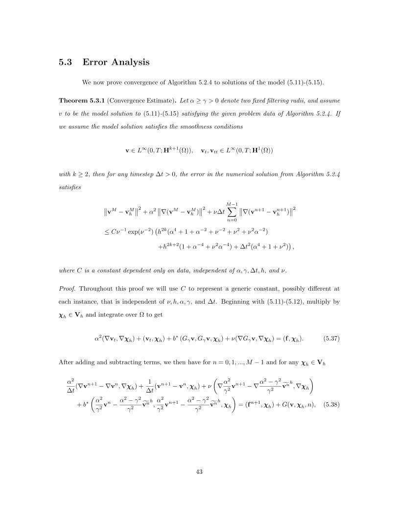
5.3 Error Analysis
We now prove convergence of Algorithm 5.2.4 to solutions of the model (5.11)-(5.15).
Theorem 5.3.1 (Convergence Estimate). Let α ≥ γ > 0 denote two fixed filtering radii, and assume
v to be the model solution to (5.11)-(5.15) satisfying the given problem data of Algorithm 5.2.4. If
we assume the model solution satisfies the smoothness conditions
v ∈ L∞(0, T ; Hk+1(Ω)), vt,vtt ∈ L∞(0, T ; H1(Ω))
with k ≥ 2, then for any timestep ∆t > 0, the error in the numerical solution from Algorithm 5.2.4
satisfies
∥∥vM − vMh∥∥2
+ α2∥∥∇(vM − vMh )
∥∥2+ ν∆t
M−1∑n=0
∥∥∇(vn+1 − vn+1h )
∥∥2
≤ Cν−1 exp(ν−2)(h2k(α4 + 1 + α−2 + ν−2 + ν2 + ν2α−2)
+h2k+2(1 + α−4 + ν2α−4) + ∆t2(α4 + 1 + ν2)),
where C is a constant dependent only on data, independent of α, γ,∆t, h, and ν.
Proof. Throughout this proof we will use C to represent a generic constant, possibly different at
each instance, that is independent of ν, h, α, γ, and ∆t. Beginning with (5.11)-(5.12), multiply by
χh ∈ Vh and integrate over Ω to get
α2(∇vt,∇χh) + (vt,χh) + b∗ (Gγv, Gγv,χh) + ν(∇Gγv,∇χh) = (f ,χh). (5.37)
After adding and subtracting terms, we then have for n = 0, 1, ...,M − 1 and for any χh ∈ Vh
α2
∆t(∇vn+1 −∇vn,∇χh) +
1
∆t(vn+1 − vn,χh) + ν
(∇α
2
γ2vn+1 −∇α
2 − γ2
γ2vn
h,∇χh
)+ b∗
(α2
γ2vn − α2 − γ2
γ2vn
h,α2
γ2vn+1 − α2 − γ2
γ2vn
h,χh
)= (fn+1,χh) +G(v,χh, n), (5.38)
43

where G(v,χh, n) is defined as
G(v,χh, n) := α2
(∇vn+1 −∇vn
∆t−∇vt(t
n+1),∇χh)
+
(vn+1 − vn
∆t− vt(t
n+1),χh
)+ ν
[(∇α
2
γ2vn+1 −∇α
2 − γ2
γ2vn
h,∇χh
)−(∇Gγvn+1,∇χh
)]−[b∗(Gγv
n+1, Gγvn+1,χh
)− b∗
(Gγv
n, Gγvn+1,χh
)]−[b∗(Gγv
n, Gγvn+1,χh
)− b∗
(Gγv
n,α2
γ2vn+1 − α2 − γ2
γ2vn,χh
)]−[b∗(Gγv
n,α2
γ2vn+1 − α2 − γ2
γ2vn,χh
)− b∗
(α2
γ2vn − α2 − γ2
γ2vn
h,α2
γ2vn+1 − α2 − γ2
γ2vn
h,χh
)]. (5.39)
From (5.38) subtract (5.20), restricting χh ∈ Vh, and denote en+1 = vn+1 − vn+1h to get
α2
∆t(∇en+1 −∇en,∇χh) + b∗
(α2
γ2vn − α2 − γ2
γ2vn
h,α2
γ2vn+1 − α2 − γ2
γ2vn
h,χh
)+
1
∆t(en+1 − en,χh)− b∗
(α2
γ2vnh −
α2 − γ2
γ2vnh
h,α2
γ2vn+1h − α2 − γ2
γ2vnh
h,χh
)+ ν
(∇α
2
γ2en+1 −∇α
2 − γ2
γ2en
h,∇χh
)= G(v,χh, n). (5.40)
Decompose en+1 = (vn+1 −wn+1h ) + (wn+1
h − vn+1h ) =: ηn+1 +φn+1
h , where wn+1h is an arbitrarily
chosen element of Vh. Then we can rewrite (5.40) as
α2
∆t(∇φn+1
h −∇φnh,∇χh) +1
∆t(φn+1
h − φnh,χh) + ν
(∇α
2
γ2φn+1h −∇α
2 − γ2
γ2φnh
h,∇χh
)= −α
2
∆t(∇ηn+1 −∇ηn,∇χh)− 1
∆t(ηn+1 − ηn,χh)− ν
(∇α
2
γ2ηn+1 −∇α
2 − γ2
γ2ηn
h,∇χh
)+G(v,χh, n)− b∗
(α2
γ2en − α2 − γ2
γ2en
h,α2
γ2vn+1 − α2 − γ2
γ2vn
h,χh
)− b∗
(α2
γ2vnh −
α2 − γ2
γ2vnh
h,α2
γ2en+1 − α2 − γ2
γ2en
h,χh
). (5.41)
Continue by choosing
χh =α2
γ2φn+1h − α2 − γ2
γ2φnh
h.
Using similar analysis techniques to those employed in Lemma 5.2.5, we can lower bound the time
44
derivative terms on the left side of (5.41) as
α2
∆t
(∇φn+1
h −∇φnh,∇α2
γ2φn+1h −∇α
2 − γ2
γ2φnh
h)
≥ α4
2γ2∆t
(∥∥∇φn+1h
∥∥2 − ‖∇φnh‖2)
+α2(α2 − γ2)
2γ2∆t
(∥∥∥∇F 1/2h φnh
∥∥∥2
−∥∥∥∇F 1/2
h φn+1h
∥∥∥2), (5.42)
and,
1
∆t
(φn+1h − φnh,
α2
γ2φn+1h − α2 − γ2
γ2φnh
h)
≥ α2
2γ2∆t
(∥∥φn+1h
∥∥2 − ‖φnh‖2)
+α2 − γ2
2γ2∆t
(∥∥∥F 1/2h φnh
∥∥∥2
−∥∥∥F 1/2
h φn+1h
∥∥∥2). (5.43)
Using the bounds (5.42)-(5.43) on (5.41) in conjunction with our choice of χh = α2
γ2φn+1h − α2−γ2
γ2 φnhh
gives
α2
2γ2∆t
(∥∥φn+1h
∥∥2 − ‖φnh‖2)
+α2 − γ2
2γ2∆t
(∥∥∥F 1/2h φnh
∥∥∥2
−∥∥∥F 1/2
h φn+1h
∥∥∥2)
+α4
2γ2∆t
(∥∥∇φn+1h
∥∥2 − ‖∇φnh‖2)
+α2(α2 − γ2)
2γ2∆t
(∥∥∥∇F 1/2h φnh
∥∥∥2
−∥∥∥∇F 1/2
h φn+1h
∥∥∥2)
+ ν
∥∥∥∥∇(α2
γ2φn+1h − α2 − γ2
γ2φnh
h)∥∥∥∥2
≤ −α2
∆t
(∇ηn+1 −∇ηn,∇
(α2
γ2φn+1h − α2 − γ2
γ2φnh
h))
− 1
∆t
(ηn+1 − ηn, α
2
γ2φn+1h − α2 − γ2
γ2φnh
h)
+G(v,χh, n)
− ν(∇(α2
γ2ηn+1 − α2 − γ2
γ2ηn
h),∇(α2
γ2φn+1h − α2 − γ2
γ2φnh
h))
− b∗(α2
γ2φnh −
α2 − γ2
γ2φnh
h,α2
γ2vn+1 − α2 − γ2
γ2vn
h,α2
γ2φn+1h − α2 − γ2
γ2φnh
h)
− b∗(α2
γ2ηn − α2 − γ2
γ2ηn
h,α2
γ2vn+1 − α2 − γ2
γ2vn
h,α2
γ2φn+1h − α2 − γ2
γ2φnh
h)
− b∗(α2
γ2vnh −
α2 − γ2
γ2vnh
h,α2
γ2φn+1h − α2 − γ2
γ2φnh
h,α2
γ2φn+1h − α2 − γ2
γ2φnh
h)
− b∗(α2
γ2vnh −
α2 − γ2
γ2vnh
h,α2
γ2ηn+1 − α2 − γ2
γ2ηn
h,α2
γ2φn+1h − α2 − γ2
γ2φnh
h). (5.44)
45
The first two terms on the right side of (5.44) are majorized as in [23]:
∣∣∣∣ 1
∆t
(ηn+1 − ηn, α
2
γ2φn+1h − α2 − γ2
γ2φnh
h)∣∣∣∣
≤ 4C2PF
ν∆t
∫ tn+1
tn‖ηt‖
2dt+
ν
16
∥∥∥∥∇(α2
γ2φn+1h − α2 − γ2
γ2φnh
h)∥∥∥∥2
, (5.45)
and
∣∣∣∣α2
∆t
(∇ηn+1 −∇ηn,∇
(α2
γ2φn+1h − α2 − γ2
γ2φnh
h))∣∣∣∣
≤ 4α4
ν∆t
∫ tn+1
tn‖∇ηt‖
2dt+
ν
16
∥∥∥∥∇(α2
γ2φn+1h − α2 − γ2
γ2φnh
h)∥∥∥∥2
. (5.46)
The viscous term on the right side of (5.44) is bounded using Cauchy-Schwarz and Young’s inequal-
ities, as well as Lemma 2.2:
∣∣∣∣ν (∇(α2
γ2ηn+1 − α2 − γ2
γ2ηn
h),∇(α2
γ2φn+1h − α2 − γ2
γ2φnh
h))∣∣∣∣
≤ ν∥∥∥∥∇(α2
γ2ηn+1 − α2 − γ2
γ2ηn
h)∥∥∥∥∥∥∥∥∇(α2
γ2φn+1h − α2 − γ2
γ2φnh
h)∥∥∥∥
≤ α2
γ2ν∥∥∇ηn+1
∥∥∥∥∥∥∇(α2
γ2φn+1h − α2 − γ2
γ2φnh
h)∥∥∥∥
+α2 − γ2
γ2ν∥∥∥∇ηnh∥∥∥∥∥∥∥∇(α2
γ2φn+1h − α2 − γ2
γ2φnh
h)∥∥∥∥
≤ ν
16
∥∥∥∥∇(α2
γ2φn+1h − α2 − γ2
γ2φnh
h)∥∥∥∥2
+ Cνα4
γ4
(∥∥∇ηn+1∥∥2
+ ‖∇ηn‖2). (5.47)
Using Lemma 2.0.2, Young’s inequality and Lemma 5.2.2, majorize the first nonlinear term in (5.44)
46

to get
∣∣∣∣−b∗(α2
γ2φnh −
α2 − γ2
γ2φnh
h,α2
γ2vn+1 − α2 − γ2
γ2vn
h,α2
γ2φn+1h − α2 − γ2
γ2φnh
h)∣∣∣∣
≤ C
(∥∥∥∥α2
γ2φnh −
α2 − γ2
γ2φnh
h∥∥∥∥1/2 ∥∥∥∥∇(α2
γ2φnh −
α2 − γ2
γ2φnh
h)∥∥∥∥1/2
·∥∥∥∥∇(α2
γ2vn+1 − α2 − γ2
γ2vn
h)∥∥∥∥∥∥∥∥∇(α2
γ2φn+1h − α2 − γ2
γ2φnh
h)∥∥∥∥)
≤ 4Cν−1
∥∥∥∥α2
γ2φnh −
α2 − γ2
γ2φnh
h∥∥∥∥∥∥∥∥∇(α2
γ2φnh −
α2 − γ2
γ2φnh
h)∥∥∥∥∥∥∥∥∇(α2
γ2vn+1 − α2 − γ2
γ2vn
h)∥∥∥∥2
+ν
16
∥∥∥∥∇(α2
γ2φn+1h − α2 − γ2
γ2φnh
h)∥∥∥∥2
≤ Cν−1 (2α2 − γ2)2
γ4‖∇φnh‖ ‖φ
nh‖(α4
γ4
∥∥∇vn+1∥∥2
+(α2 − γ2)2
γ4
∥∥∥∇vnh∥∥∥2)
+ν
16
∥∥∥∥∇(α2
γ2φn+1h − α2 − γ2
γ2φnh
h)∥∥∥∥2
≤ Cν−2α8(2α2 − γ2)4
γ16‖φnh‖
2 ∥∥∇vn+1∥∥4
+ Cν−2 (α2 − γ2)4(2α2 − γ2)4
γ16‖φnh‖
2 ‖∇vn‖4
+ν
16‖∇φnh‖
2+
ν
16
∥∥∥∥∇(α2
γ2φn+1h − α2 − γ2
γ2φnh
h)∥∥∥∥2
≤ ν
16
∥∥∥∥∇(α2
γ2φn+1h − α2 − γ2
γ2φnh
h)∥∥∥∥2
+ν
16‖∇φnh‖
2+ Cν−2α
16
γ16‖φnh‖
2(∥∥∇vn+1
∥∥4+ ‖∇vn‖4
).
(5.48)
47

Using Lemma 2.0.2 and Young’s inequality on the second nonlinear term in (5.44) gives
∣∣∣∣−b∗(α2
γ2ηn − α2 − γ2
γ2ηn
h,α2
γ2vn+1 − α2 − γ2
γ2vn
h,α2
γ2φn+1h − α2 − γ2
γ2φnh
h)∣∣∣∣
≤ C∥∥∥∥∇(α2
γ2ηn − α2 − γ2
γ2ηn
h)∥∥∥∥∥∥∥∥∇(α2
γ2vn+1 − α2 − γ2
γ2vn
h)∥∥∥∥∥∥∥∥∇(α2
γ2φn+1h − α2 − γ2
γ2φnh
h)∥∥∥∥
≤ C 2α2 − γ2
γ2‖∇ηn‖
∥∥∥∥∇(α2
γ2vn+1 − α2 − γ2
γ2vn
h)∥∥∥∥∥∥∥∥∇(α2
γ2φn+1h − α2 − γ2
γ2φnh
h)∥∥∥∥
≤ Cα2(2α2 − γ2)
γ4‖∇ηn‖
∥∥∇vn+1∥∥ ∥∥∥∥∇(α2
γ2φn+1h − α2 − γ2
γ2φnh
h)∥∥∥∥
+ C(α2 − γ2)(2α2 − γ2)
γ4‖∇ηn‖ ‖∇vn‖
∥∥∥∥∇(α2
γ2φn+1h − α2 − γ2
γ2φnh
h)∥∥∥∥
≤ ν
16
∥∥∥∥∇(α2
γ2φn+1h − α2 − γ2
γ2φnh
h)∥∥∥∥2
+ Cν−1α4(2α2 − γ2)2
γ8‖∇ηn‖2
∥∥∇vn+1∥∥2
+ Cν−1 (α2 − γ2)2(2α2 − γ2)2
γ8‖∇ηn‖2 ‖∇vn‖2
≤ ν
16
∥∥∥∥∇(α2
γ2φn+1h − α2 − γ2
γ2φnh
h)∥∥∥∥2
+ Cν−1α8
γ8‖∇ηn‖2
(∥∥∇vn+1∥∥2
+ ‖∇vn‖2). (5.49)
By Lemma 2.0.2, the third nonlinear term in (5.44) vanishes. Finally, the fourth nonlinear term is
bounded in the same manner as in (5.49)
∣∣∣∣−b∗(α2
γ2vnh −
α2 − γ2
γ2vnh
h,α2
γ2ηn+1 − α2 − γ2
γ2ηn
h,α2
γ2φn+1h − α2 − γ2
γ2φnh
h)∣∣∣∣
≤ ν
16
∥∥∥∥∇(α2
γ2φn+1h − α2 − γ2
γ2φnh
h)∥∥∥∥2
+ Cν−1α8
γ8‖∇vnh‖
2(∥∥∇ηn+1
∥∥2+ ‖∇ηn‖2
). (5.50)
Applying the bounds (5.45)-(5.50) to equation (5.44) yields
α2
2γ2∆t
(∥∥φn+1h
∥∥2 − ‖φnh‖2)
+α2 − γ2
2γ2∆t
(∥∥∥F 1/2h φnh
∥∥∥2
−∥∥∥F 1/2
h φn+1h
∥∥∥2)
+α4
2γ2∆t
(∥∥∇φn+1h
∥∥2 − ‖∇φnh‖2)
+α2(α2 − γ2)
2γ2∆t
(∥∥∥∇F 1/2h φnh
∥∥∥2
−∥∥∥∇F 1/2
h φn+1h
∥∥∥2)
+10ν
16
∥∥∥∥∇(α2
γ2φn+1h − α2 − γ2
γ2φnh
h)∥∥∥∥2
≤ ν
16‖∇φnh‖
2+
4C2PF
ν∆t
∫ tn+1
tn‖ηt‖
2dt
+4α4
ν∆t
∫ tn+1
tn‖∇ηt‖
2dt+ Cν
α4
γ4
(∥∥∇ηn+1∥∥2
+ ‖∇ηn‖2)
+ Cν−2α16
γ16‖φnh‖
2(∥∥∇vn+1
∥∥4+ ‖∇vn‖4
)+ Cν−1α
8
γ8‖∇ηn‖2
(∥∥∇vn+1∥∥2
+ ‖∇vn‖2)
+ Cν−1α8
γ8‖∇vnh‖
2(∥∥∇ηn+1
∥∥2+ ‖∇ηn‖2
)+
∣∣∣∣G(v,α2
γ2φn+1h − α2 − γ2
γ2φnh
h, n
)∣∣∣∣ . (5.51)
48

We will now continue by majorizing
∣∣∣∣G(v,α2
γ2φn+1h − α2 − γ2
γ2φnh
h, n
)∣∣∣∣ ,as defined in (5.39) with χh = α2
γ2φn+1h − α2−γ2
γ2 φnhh. The first term of (5.39) is bounded using
standard estimates based on Taylor series
α2
(∇vn+1 −∇vn
∆t−∇vt(t
n+1),∇(α2
γ2φn+1h − α2 − γ2
γ2φnh
h))
≤ ν
16
∥∥∥∥∇(α2
γ2φn+1h − α2 − γ2
γ2φnh
h)∥∥∥∥2
+ 2∆t2α4ν−1 ‖vtt‖2L∞(tn,tn+1,H1(Ω)) . (5.52)
The second term of G is bounded in the same manner
(vn+1 − vn
∆t− vt(t
n+1),α2
γ2φn+1h − α2 − γ2
γ2φnh
h)
≤ ν
16
∥∥∥∥∇(α2
γ2φn+1h − α2 − γ2
γ2φnh
h)∥∥∥∥2
+ 2∆t2C2PF ν
−1 ‖vtt‖2L∞(tn,tn+1,H1(Ω)) . (5.53)
Using Cauchy-Schwarz and Young’s inequalities on the third term of (5.39) yields
∣∣∣∣ν (∇(α2
γ2vn+1 − α2 − γ2
γ2vn
h)−∇Gγvn+1,∇
(α2
γ2φn+1h − α2 − γ2
γ2φnh
h))∣∣∣∣
=
∣∣∣∣ν(α2 − γ2)
γ2
(∇(vn+1 − vn
h),∇(α2
γ2φn+1h − α2 − γ2
γ2φnh
h))∣∣∣∣
=
∣∣∣∣ν(α2 − γ2)
γ2
(∇(vn+1 − vn
),∇(α2
γ2φn+1h − α2 − γ2
γ2φnh
h))
+ν(α2 − γ2)
γ2
(∇(vn − vn
h),∇(α2
γ2φn+1h − α2 − γ2
γ2φnh
h))∣∣∣∣
≤ ν
16
∥∥∥∥∇(α2
γ2φn+1h − α2 − γ2
γ2φnh
h)∥∥∥∥2
+ Cν(α2 − γ2)2
γ4
(∥∥∥∇(vn+1 − vn)∥∥∥2
+∥∥∥∇(vn − vn
h)∥∥∥2
).
Using estimates based on Taylor series as well as Lemma 5.2.3 to bound the difference between
49

continuous and discrete filters, we then see
∣∣∣∣ν (∇(α2
γ2vn+1 − α2 − γ2
γ2vn
h)−∇Gγvn+1,∇
(α2
γ2φn+1h − α2 − γ2
γ2φnh
h))∣∣∣∣
≤ ν
16
∥∥∥∥∇(α2
γ2φn+1h − α2 − γ2
γ2φnh
h)∥∥∥∥2
+ Cνα4
γ4∆t2 ‖vt‖2L∞(tn,tn+1,H1(Ω))
+ Cνα4
γ6(γ−2h2k+2 + h2k) ‖vn‖2Hk+1(Ω) . (5.54)
To bound the fourth term of G, we use Lemma 2.0.2, Young’s inequality, and Taylor’s theorem to
arrive at
∣∣∣∣b∗(Gγvn+1, Gγvn+1,
α2
γ2φn+1h − α2 − γ2
γ2φnh
h)− b∗
(Gγv
n, Gγvn+1,
α2
γ2φn+1h − α2 − γ2
γ2φnh
h)∣∣∣∣
=
∣∣∣∣b∗(Gγ(vn+1 − vn), Gγvn+1,
α2
γ2φn+1h − α2 − γ2
γ2φnh
h)∣∣∣∣
≤∥∥∥∥∇(α2
γ2φn+1h − α2 − γ2
γ2φnh
h)∥∥∥∥∥∥∇Gγ(vn+1 − vn)
∥∥∥∥∇Gγvn+1∥∥
≤ ν
16
∥∥∥∥∇(α2
γ2φn+1h − α2 − γ2
γ2φnh
h)∥∥∥∥2
+ Cν−1∥∥∇Gγ(vn+1 − vn)
∥∥2 ∥∥∇Gγvn+1∥∥2
≤ ν
16
∥∥∥∥∇(α2
γ2φn+1h − α2 − γ2
γ2φnh
h)∥∥∥∥2
+ Cν−1α8
γ8
∥∥∇(vn+1 − vn)∥∥2 ∥∥∇vn+1
∥∥2
≤ ν
16
∥∥∥∥∇(α2
γ2φn+1h − α2 − γ2
γ2φnh
h)∥∥∥∥2
+ Cν−1α8
γ8∆t2 ‖vt‖2L∞(tn,tn+1,H1(Ω))
∥∥∇vn+1∥∥2. (5.55)
The same techniques are used to bound the fifth term in (5.39)
∣∣∣∣b∗(Gγvn, Gγvn+1,α2
γ2φn+1h − α2 − γ2
γ2φnh
h)
−b∗(Gγv
n,α2
γ2vn+1 − α2 − γ2
γ2vn,
α2
γ2φn+1h − α2 − γ2
γ2φnh
h)∣∣∣∣
=
∣∣∣∣b∗(Gγvn, α2 − γ2
γ2
(vn − vn+1
),α2
γ2φn+1h − α2 − γ2
γ2φnh
h)∣∣∣∣
≤ ν
16
∥∥∥∥∇(α2
γ2φn+1h − α2 − γ2
γ2φnh
h)∥∥∥∥2
+ Cν−1 (α2 − γ2)2
γ4
∥∥∥∇(vn − vn+1)∥∥∥2
‖∇Gγvn‖2
≤ ν
16
∥∥∥∥∇(α2
γ2φn+1h − α2 − γ2
γ2φnh
h)∥∥∥∥2
+ Cν−1α8
γ8∆t2 ‖vt‖2L∞(tn,tn+1,H1(Ω)) ‖∇vn‖2 . (5.56)
50

For the sixth term in (5.39), we start by using Lemma 2.0.2 and Lemma 5.2.2
∣∣∣∣b∗(Gγvn, α2
γ2vn+1 − α2 − γ2
γ2vn,
α2
γ2φn+1h − α2 − γ2
γ2φnh
h)
−b∗(α2
γ2vn − α2 − γ2
γ2vn
h,α2
γ2vn+1 − α2 − γ2
γ2vn
h,α2
γ2φn+1h − α2 − γ2
γ2φnh
h)∣∣∣∣
=
∣∣∣∣b∗(α2 − γ2
γ2
(vn
h − vn),α2
γ2vn+1 − α2 − γ2
γ2vn
h,α2
γ2φn+1h − α2 − γ2
γ2φnh
h)
−b∗(Gγv
n,α2 − γ2
γ2
(vn − vn
h),α2
γ2φn+1h − α2 − γ2
γ2φnh
h)∣∣∣∣
≤ Cα2 − γ2
γ2
∥∥∥∇(vnh − vn)∥∥∥∥∥∥∥∇(α2
γ2φn+1h − α2 − γ2
γ2φnh
h)∥∥∥∥
·(∥∥∥∥∇(α2
γ2vn+1 − α2 − γ2
γ2vn
h)∥∥∥∥+ ‖∇Gγvn‖
)≤ Cα
2(α2 − γ2)
γ4
∥∥∥∇(vnh − vn
)∥∥∥∥∥∥∥∇(α2
γ2φn+1h − α2 − γ2
γ2φnh
h)∥∥∥∥ (∥∥∇vn+1
∥∥+ ‖∇vn‖).
Using Young’s inequality and Lemma 5.2.3 we then get
∣∣∣∣b∗(Gγvn, α2
γ2vn+1 − α2 − γ2
γ2vn,
α2
γ2φn+1h − α2 − γ2
γ2φnh
h)
−b∗(α2
γ2vn − α2 − γ2
γ2vn
h,α2
γ2vn+1 − α2 − γ2
γ2vn
h,α2
γ2φn+1h − α2 − γ2
γ2φnh
h)∣∣∣∣
≤ ν
16
∥∥∥∥∇(α2
γ2φn+1h − α2 − γ2
γ2φnh
h)∥∥∥∥2
+ Cν−1α4(α2 − γ2)2
γ8
∥∥∥∇(vnh − vn
)∥∥∥2 (∥∥∇vn+1∥∥+ ‖∇vn‖
)2≤ ν
16
∥∥∥∥∇(α2
γ2φn+1h − α2 − γ2
γ2φnh
h)∥∥∥∥2
+ Cν−1 α8
γ10
(γ−2h2k+2 + h2k
)‖vn‖2Hk+1(Ω)
(∥∥∇vn+1∥∥+ ‖∇vn‖
)2. (5.57)
51

Using the bounds (5.52)-(5.57) on equation (5.51), we get
α2
2γ2∆t
(∥∥φn+1h
∥∥2 − ‖φnh‖2)
+α2 − γ2
2γ2∆t
(∥∥∥F 1/2h φnh
∥∥∥2
−∥∥∥F 1/2
h φn+1h
∥∥∥2)
+α4
2γ2∆t
(∥∥∇φn+1h
∥∥2 − ‖∇φnh‖2)
+α2(α2 − γ2)
2γ2∆t
(∥∥∥∇F 1/2h φnh
∥∥∥2
−∥∥∥∇F 1/2
h φn+1h
∥∥∥2)
+ν
4
∥∥∥∥∇(α2
γ2φn+1h − α2 − γ2
γ2φnh
h)∥∥∥∥2
≤ ν
16‖∇φnh‖
2+
4C2PF
ν∆t
∫ tn+1
tn‖ηt‖
2dt
+4α4
ν∆t
∫ tn+1
tn‖∇ηt‖
2dt+ Cν
α4
γ4
(∥∥∇ηn+1∥∥2
+ ‖∇ηn‖2)
+ Cν−2α16
γ16‖φnh‖
2(∥∥∇vn+1
∥∥4+ ‖∇vn‖4
)+ Cν−1α
8
γ8‖∇ηn‖2
(∥∥∇vn+1∥∥2
+ ‖∇vn‖2)
+ Cν−1α8
γ8‖∇vnh‖
2(∥∥∇ηn+1
∥∥2+ ‖∇ηn‖2
)+ Cν−1∆t2α4 ‖vtt‖2L∞(tn,tn+1,H1(Ω)) + Cν−1∆t2 ‖vtt‖2L∞(tn,tn+1,H1(Ω))
+ Cν∆t2α4
γ4‖vt‖2L∞(tn,tn+1,H1(Ω)) + Cν
α4
γ6(γ−2h2k+2 + h2k) ‖vn‖2Hk+1(Ω)
+ Cν−1∆t2α8
γ8‖vt‖2L∞(tn,tn+1,H1(Ω))
∥∥∇vn+1∥∥2
+ Cν−1∆t2α8
γ8‖vt‖2L∞(tn,tn+1,H1(Ω)) ‖∇vn‖2
+ Cν−1 α8
γ10
(γ−2h2k+2 + h2k
)‖vn‖2Hk+1(Ω)
(∥∥∇vn+1∥∥+ ‖∇vn‖
)2. (5.58)
52
Multiplying through by 2∆t and summing from n = 0 to M − 1 yields
α2
γ2
(∥∥∥φMh ∥∥∥2
−∥∥φ0
h
∥∥)+α2 − γ2
γ2
(∥∥∥F 1/2h φ0
h
∥∥∥2
−∥∥∥F 1/2
h φMh
∥∥∥2)
+α4
γ2
(∥∥∥∇φMh ∥∥∥2
−∥∥∇φ0
h
∥∥2)
+α2(α2 − γ2)
γ2
(∥∥∥∇F 1/2h φ0
h
∥∥∥2
−∥∥∥∇F 1/2
h φMh
∥∥∥2)
+ν∆t
2
M−1∑n=0
∥∥∥∥∇(α2
γ2φn+1h − α2 − γ2
γ2φnh
h)∥∥∥∥2
≤ ν∆t
8
M−1∑n=0
‖∇φnh‖2
+ Cν−1
∫ T
0
‖ηt‖2dt+ Cν−1α4
∫ T
0
‖∇ηt‖2dt
+ Cν∆tα4
γ4
M−1∑n=0
(∥∥∇ηn+1∥∥2
+ ‖∇ηn‖2)
+ Cν−2∆tα16
γ16
M−1∑n=0
‖φnh‖2(∥∥∇vn+1
∥∥4+ ‖∇vn‖4
)+ Cν−1∆t
α8
γ8
M−1∑n=0
‖∇ηn‖2(∥∥∇vn+1
∥∥2+ ‖∇vn‖2
)+ Cν−1∆t
α8
γ8
M−1∑n=0
‖∇vnh‖2(∥∥∇ηn+1
∥∥2+ ‖∇ηn‖2
)+ Cν−1∆t3α4
M−1∑n=0
‖vtt‖2L∞(tn,tn+1,H1(Ω)) + Cν−1∆t3M−1∑n=0
‖vtt‖2L∞(tn,tn+1,H1(Ω))
+ Cν∆t3α4
γ4
M−1∑n=0
‖vt‖2L∞(tn,tn+1,H1(Ω)) + Cν∆tα4
γ6(γ−2h2k+2 + h2k)
M−1∑n=0
‖vn‖2Hk+1(Ω)
+ Cν−1∆t3α8
γ8
M−1∑n=0
‖vt‖2L∞(tn,tn+1,H1(Ω))
∥∥∇vn+1∥∥2
+ Cν−1∆t3α8
γ8
M−1∑n=0
‖vt‖2L∞(tn,tn+1,H1(Ω)) ‖∇vn‖2
+ Cν−1∆tα8
γ10(γ−2h2k+2 + h2k)
M−1∑n=0
‖vn‖2Hk+1(Ω)
(∥∥∇vn+1∥∥+ ‖∇vn‖
)2. (5.59)
Note that our assumption of v0 ∈ Vh implies φ0h = 0. Using this and assumptions on the regularity
53

of the model solution, (5.59) becomes
α2
γ2
∥∥∥φMh ∥∥∥2
− α2 − γ2
γ2
∥∥∥F 1/2h φMh
∥∥∥2
+α4
γ2
∥∥∥∇φMh ∥∥∥2
− α2(α2 − γ2)
γ2
∥∥∥∇F 1/2h φMh
∥∥∥2
+ν∆t
2
M−1∑n=0
∥∥∥∥∇(α2
γ2φn+1h − α2 − γ2
γ2φnh
h)∥∥∥∥2
≤ ν∆t
8
M−1∑n=0
‖∇φnh‖2
+ Cν−1
∫ T
0
‖ηt‖2dt
+ Cν−1α4
∫ T
0
‖∇ηt‖2dt+ Cν∆t
α4
γ4
M−1∑n=0
(∥∥∇ηn+1∥∥2
+ ‖∇ηn‖2)
+ Cν−2∆tα16
γ16
M−1∑n=0
‖φnh‖2
+ Cν−1∆tα8
γ8
M−1∑n=0
‖∇ηn‖2 + Cν−1∆tα8
γ8
M−1∑n=0
‖∇vnh‖2(∥∥∇ηn+1
∥∥2+ ‖∇ηn‖2
)+ Cν−1T∆t2α4
+ Cν−1T∆t2 + CνT∆t2α4
γ4+ CνT
α4
γ6
(γ−2h2k+2 + h2k
)+ Cν−1T∆t2
α8
γ8
+ Cν−1Tα8
γ10
(γ−2h2k+2 + h2k
). (5.60)
With regularity assumptions and interpolation estimates, (5.60) becomes
α2
γ2
∥∥∥φMh ∥∥∥2
− α2 − γ2
γ2
∥∥∥F 1/2h φMh
∥∥∥2
+α4
γ2
∥∥∥∇φMh ∥∥∥2
− α2(α2 − γ2)
γ2
∥∥∥∇F 1/2h φMh
∥∥∥2
+ν∆t
2
M−1∑n=0
∥∥∥∥∇(α2
γ2φn+1h − α2 − γ2
γ2φnh
h)∥∥∥∥2
≤ ν∆t
8
M−1∑n=0
‖∇φnh‖2
+ Cν−2∆tα16
γ16
M−1∑n=0
‖φnh‖2
+ Cν−1T
(h2k+2 + α4h2k +
α8
γ8h2k + ∆t2α4 + ∆t2 + ∆t2
α8
γ8+α8
γ10(γ−2h2k+2 + h2k)
)+ CνT
(α4
γ4h2k + ∆t2
α4
γ4+α4
γ6(γ−2h2k+2 + h2k)
)+ Cν−1∆t
α8
γ8h2k
M−1∑n=0
‖∇vnh‖2. (5.61)
We can lower bound the viscous term in the same fashion as in Lemma 5.2.5 to get
ν∆t
2
M−1∑n=0
∥∥∥∥∇(α2
γ2φn+1h − α2 − γ2
γ2φnh
h)∥∥∥∥2
≥ ν∆t
2
M−1∑n=0
(∥∥∇φn+1h
∥∥2+α2 − γ2
γ2(∥∥∇φn+1
h
∥∥2 − ‖∇φnh‖2)
)
=ν∆t
2
M−1∑n=0
∥∥∇φn+1h
∥∥2+ν∆t(α2 − γ2)
2γ4
∥∥∥∇φMh ∥∥∥2
. (5.62)
54

Combining (5.61) and (5.62), and using Lemma 5.2.5 and (φh,φ) ≤ ‖φh‖
2gives
∥∥∥φMh ∥∥∥2
+ α2∥∥∥∇φMh ∥∥∥2
+ν∆t
2
M−1∑n=0
∥∥∇φn+1h
∥∥2 ≤ ν∆t
8
M−1∑n=0
‖∇φnh‖2
+ Cν−2∆tα16
γ16
M−1∑n=0
‖φnh‖2
+ Cν−1
(h2k
(α4 +
α8
γ8+α8
γ10+ ν−2α
8
γ8
)+ h2k+2
(1 +
α8
γ12
)+ ∆t2
(α4 + 1 +
α8
γ8
))+ Cν
(h2k
(α4
γ4+α4
γ6
)+α4
γ8h2k+2 +
α4
γ4∆t2
). (5.63)
Subtracting ν∆t8
M−1∑n=0
‖∇φnh‖2
from both sides yields
∥∥∥φMh ∥∥∥2
+ α2∥∥∥∇φMh ∥∥∥2
+3ν∆t
8
M−1∑n=0
∥∥∇φn+1h
∥∥2 ≤ Cν−2∆tα16
γ16
M−1∑n=0
‖φnh‖2
+ Cν−1
(h2k
(α4 +
α8
γ8+α8
γ10+ ν−2α
8
γ8
)+ h2k+2
(1 +
α8
γ12
)+ ∆t2
(α4 + 1 +
α8
γ8
))+ Cν
(h2k
(α4
γ4+α4
γ6
)+α4
γ8h2k+2 +
α4
γ4∆t2
). (5.64)
Applying the discrete Gronwall lemma we see, for any ∆t > 0,
∥∥∥φMh ∥∥∥2
+ α2∥∥∥∇φMh ∥∥∥2
+ ν∆t
M−1∑n=0
∥∥∇φn+1h
∥∥2
≤ Cν−1 exp
(ν−2α
16
γ16
)[h2k
(α4 +
α8
γ8+α8
γ10+ ν−2α
8
γ8+ ν2α
4
γ4+ ν2α
4
γ6
)+h2k+2
(1 +
α8
γ12+ ν2α
4
γ8
)+ ∆t2
(α4 + 1 +
α8
γ8+ ν2α
4
γ4
)]. (5.65)
Finally, using our assumption that α = C0γ gives us the bound
∥∥∥φMh ∥∥∥2
+ α2∥∥∥∇φMh ∥∥∥2
+ ν∆t
M−1∑n=0
∥∥∇φn+1h
∥∥2(5.66)
≤ Cν−1 exp(ν−2)(h2k(α4 + 1 + α−2 + ν−2 + ν2 + ν2α−2)
+h2k+2(1 + α−4 + ν2α−4) + ∆t2(α4 + 1 + ν2)).
Using the triangle inequality now finishes the proof.
55

5.4 Numerical Results
This section presents two benchmark numerical experiments chosen to evaluate the accuracy
of Algorithm 5.2.4 on flow problems with complex behaviours. In both experiments, a resolved
solution is generated by computing the NSE directly on a fine triangular mesh, using the fully implicit
Crank-Nicolson finite element method (as in [46]). Solutions are then generated for Algorithm 5.2.4
using various values for α and γ. We hope to see an increase in accuracy in RMDM solutions
generated with α > γ as opposed to those generated with α = γ (i.e. those with no deconvolution).
All computations were performed using the open-source software FreeFem++ [39].
5.4.1 2D Channel flow over a backward-facing step
Fine mesh -144, 456 dof
Coarse mesh - 15, 970 dof
Figure 5.1: Fine mesh used for the resolved NSE solution and the coarse mesh used for the RMDMapproximations.
The first experiment we present is a well-known benchmark flow problem consisting of
2D channel flow over a backward-facing step. Once the flow passes over the step, the shear-layer
separates from the bottom wall, causing complex flow behaviour behind the step. It has been well
documented that the subsequent length until the flow reattaches to the wall is dependent upon both
56

the Reynolds number and the expansion ratio of the channel (see e.g. [5] and [44]). The domain Ω
consists of a 40h× 10h channel with a step of height h and length 10h running along the bottom of
the channel, as seen in Figure 5.1. Our choice of channel parameterization yields an expansion ratio
of 10/9. For our experiment we employed a step height of h = 1. Flow entering the channel on the
left is assumed to satisfy the parabolic Dirichlet boundary condition
u =
4(y − 1)(10− y)/81
0
,
while zero-traction boundary conditions are enforced on flow exiting the channel on the right. No-
slip boundary conditions are assumed on all other boundaries. All computations were performed
using Reynolds number Re = 1000, a time-step of ∆t = 0.01, and with the flow started from rest at
T = 0.
The reference NSE solution was computed using TH (P2, P1) elements on a mesh providing
144, 456 combined degrees of freedom for the velocity and pressure (see Figure 5.1). The computed
reference solution reaches a steady state by T = 200, with a steady-state reattachment length of
approximately 17.5 units, which agrees with the experimental results found in [5]. A plot of the
velocity streamlines and speed contours of the solution at T = 200 can be seen in Figure 5.2.
Solutions to Algorithm 5.2.4 were computed using TH elements on a coarse mesh providing
15, 970 combined degrees of freedom for the velocity and pressure (see Figure 5.1). We began by
computing Algorithm 5.2.4 with α = γ = 0.125, i.e. with no deconvolution. A plot of the streamlines
and speed contours of the solution at T = 200 is shown in Figure 5.2. It is clear that the RMDM
without deconvolution produces a solution that is incorrect. The three eddies present behind the
step have yet to merge into one large eddy. However, when γ is lowered to 0.06, the RMDM solution
looks very close to the reference solution. From Figure 5.2 we can clearly see that both the number
of eddies present behind the step and the reattachment length both seem to be correct. Hence, by
reducing γ we can produce a substantially more accurate approximation.
5.4.2 2D Channel flow with a contraction and two outlets
The second benchmark experiment we present is channel flow with a contraction, one inlet
on the left of the channel, and two outlets at the top and the right of the channel (as seen in Figure
57

5.3). This problem was first studied by Heywood et al. [41]. Flow entering the channel satisfies the
parabolic profile
u =
4y(1− y)
0
.
Zero-traction boundary conditions are enforced on both outflow boundaries, and no-slip boundary
conditions are enforced on all wall boundaries. All computations were performed with Re = 1000,
flow starting at rest at T = 0, and an end time of T = 4.
The reference NSE solution was computed using TH (P2, P1) elements on a fine mesh
providing 260, 378 combined degrees of freedom for the velocity and the pressure (see Figure 5.3),
and with a time-step of ∆t = 0.005. Speed contours of the resolved solution are shown in Figure
5.4. Note that the flow speeds up in the contraction, and seems to oscillate up and down on the
right side of the channel. Additionally, the flow seems to remain in a single stream once it passes
the contraction, although by T = 4, we also see the appearance of smaller flow structures near the
right outflow boundary.
Solutions to Algorithm 5.2.4 were computed using TH elements with a time-step of ∆t = 0.01
on the coarse mesh pictured in 5.4, providing 10, 820 degrees of freedom for the velocity and pressure.
Figure 5.4 shows a plot of the speed contours of the solution of our proposed method for the RMDM
with α = γ = 0.05 (no deconvolution). It is clear from the plots that this velocity solution does not
accurately capture the shape of the flow after the contraction. We also see flow leaving the channel
through the top outlet, which is not present in the resolved NSE solution plot. However, when we
recompute with α = 0.05 and γ = 0.03, the velocity solution (pictured in Figure 5.4) much more
accurately captures the shape of the flow after the contraction. Additionally, we see very little fluid
exiting the channel through the top outlet, which agrees with our “true” resolved solution. Both
solutions seem to partially capture the formation of smaller flow structures near the right outlet.
Again, we see that the solution to Algorithm 5.2.4 with α > γ is much closer to the resolved NSE
solution than that computed with no deconvolution.
58
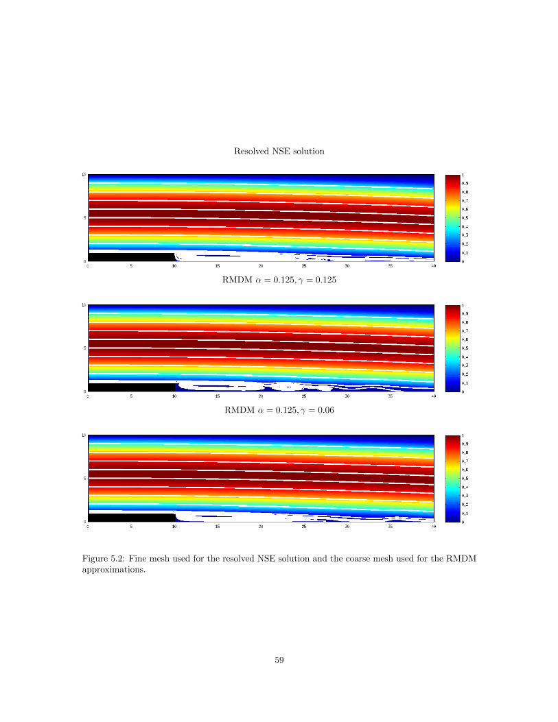
Resolved NSE solution
RMDM α = 0.125, γ = 0.125
RMDM α = 0.125, γ = 0.06
Figure 5.2: Fine mesh used for the resolved NSE solution and the coarse mesh used for the RMDMapproximations.
59

Contraction domain
Fine mesh - 260, 378 dof
Coarse Mesh - 10, 820 dof
Figure 5.3: Diagram of the contraction domain, along with the fine and coarse meshes used in thecomputations for the contraction problem.
60
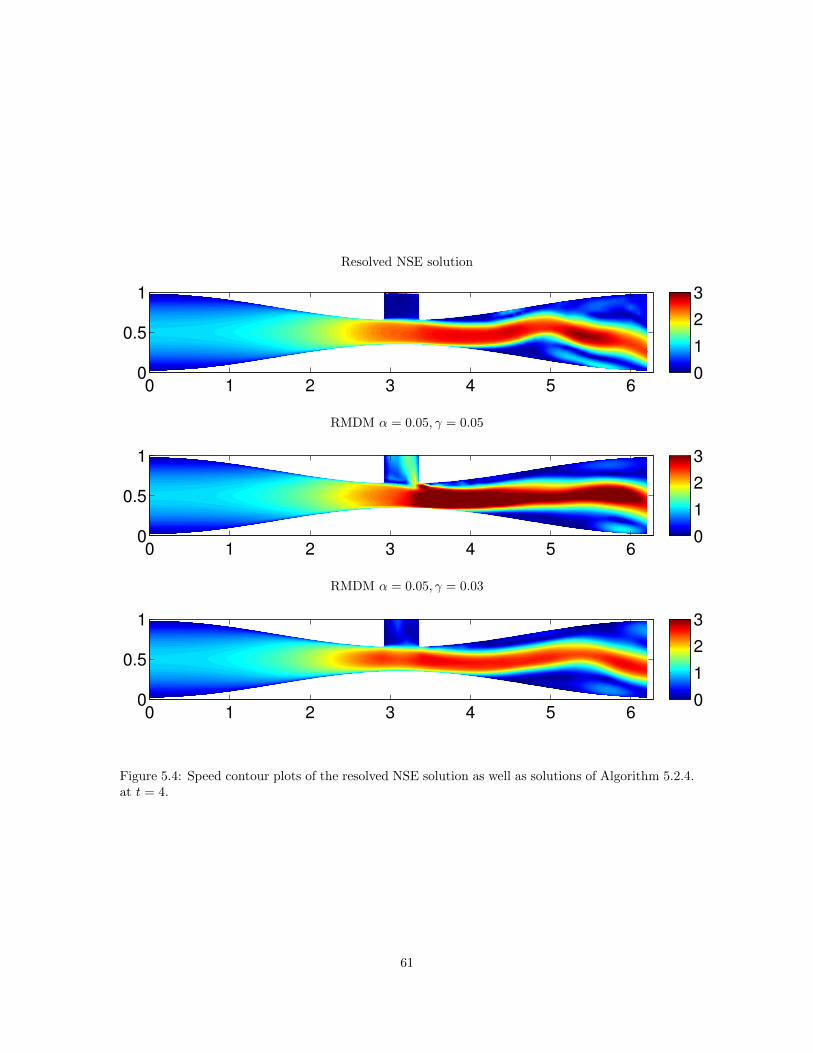
Resolved NSE solution
0 1 2 3 4 5 60
0.5
1
0
1
2
3
RMDM α = 0.05, γ = 0.05
0 1 2 3 4 5 60
0.5
1
0
1
2
3
RMDM α = 0.05, γ = 0.03
0 1 2 3 4 5 60
0.5
1
0
1
2
3
Figure 5.4: Speed contour plots of the resolved NSE solution as well as solutions of Algorithm 5.2.4.at t = 4.
61

Chapter 6
Analysis and approximation of the
Cross model for quasi-Newtonian
flows with defective boundary
conditions
In this chapter we study a numerical method for the Cross model for generalized-Newtonian
fluids with flow rate boundary conditions. The defective boundary problem is formulated as a
constrained optimal control problem, where a flow balance is enforced on the inflow and outflow
boundaries using a Neumann control. The control problem is analyzed for an existence result and
the Lagrange multiplier rule. Finally, a decoupling solution algorithm is presented and numerical
experiments are provided to validate robustness of the algorithm.
62

6.1 Modeling Equations and Preliminaries
The Cross model [16] for generalized-Newtonian fluids characterizes viscosity ν as a function
of shear rate |D(u)| = (D(u) : D(u))12 ,
ν(|D(u)|) := ν∞ +(ν0 − ν∞)
1 + (λ|D(u)|)2−r , (6.1)
where λ > 0 is a time constant, 1 ≤ r ≤ 2 is a dimensionless rate constant and ν∞ and ν0
denote limiting viscosity values at an infinite and zero shear rate, respectively, assumed to satisfy
0 ≤ ν∞ ≤ ν0. Throughout this chapter we will restrict our focus to the case where λ = 1.
We will suppose the boundary of Ω consists of inflow and outflow boundaries Si, i =
1, 2, ...,m, and a wall boundary Γ = ∂Ω \ S, where S = ∪mi=1Si. Consider, as a model problem
for steady, incompressible generalized-Newtonian flow, the two-field Cross model given by
−∇ · [(ν∞ + (ν0 − ν∞)(1 + |D(u)|2−r)−1)D(u)] +∇p = f in Ω, (6.2)
∇ · u = 0 in Ω, (6.3)
u = 0 on Γ, (6.4)
We will consider the defective boundary problem where flow rates are specified on the inflow and
outflow boundaries
Si :
∫Si
u · n dS = Qi for i = 1, 2, ...,m, (6.5)
where
m∑i=1
Qi = 0 to satisfy the incompressibility condition.
For our choice of velocity space we will choose the subspace
X := v ∈ H1(Ω) |v = 0 on Γ,
and for our pressure space we will take Q := L2(Ω). Let σ denote the shear stress (tensor) of the
fluid. If the flow rate boundary conditions (6.5) are replaced by the well defined Neumann boundary
conditions
(σ − pI) · n = gi on Si for i = 1, 2, ...,m, (6.6)
63
then the variational formulation of the problem is: Find (u, p) ∈ X×Q satisfying, for any (v, q) ∈
X×Q,
ν∞(D(u), D(v)) + (ν0 − ν∞)((1 + |D(u)|2−r)−1D(u), D(v))
−(p,∇ · v) = (f ,v) + (g,v)S , (6.7)
(∇ · u, q) = 0. (6.8)
Define the mapping A : X→ X∗ as follows: For any u ∈ X, Au satisfies
〈Au,v〉 = ν∞(D(u), D(v)) + (ν0 − ν∞)((1 + |D(u)|2−r)−1D(u), D(v)) ∀ v ∈ X. (6.9)
In [8] it was shown that for any u ∈ X, Au is strongly monotone and Lipschitz continuous, i.e. there
exist constants m,M > 0 such that Au satisfies
〈Au−Av,u− v〉 ≥ m ‖u− v‖21 ∀ v ∈ X, (6.10)
and
‖Au−Av‖∗ ≤M ‖u− v‖1 ∀ v ∈ X. (6.11)
Note also that our choice of velocity and pressure spaces satisfy the inf-sup condition:
infq∈Q
supv∈X
(q,∇ · v)
‖v‖1 ‖q‖≥ C > 0. (6.12)
Then the existence of a unique solution to (6.7)-(6.8) follows from the strong monotonicity (6.10)
and continuity (6.11) of A, as well as the inf-sup condition. Additionally, for some C > 0 we have
the following a priori bound on solutions of the variational problem (6.7)-(6.8) [14]:
‖u‖1 + ‖p‖ ≤ C(‖f‖∗ + ‖g‖L2(S)). (6.13)
64

6.2 The Optimal Control Problem
6.2.1 Problem formulation
We continue by formulating the defective boundary problem (6.2)-(6.5) as an optimal control
problem for flow rate matching. We choose as our control the normal component of the total stress
on the defective boundaries
g := gi := (σ − pI) · n on Si, i = 1, 2, ...,m, (6.14)
where g ∈ G := L2(S). We want to minimize the penalized functional
J (u, p,g) :=1
2
m∑i=1
(∫Si
u · n dSi −Qi)2
+ε
2
∫S
|g|2dS, (6.15)
where the penalty parameter ε is a positive constant that measures the relative importance of the
last term in (6.15). If we define the admissibility set as
Uad := (u, p,g) ∈ X×Q×G : J (u, p,g) <∞, (6.16)
then the defective boundary problem (6.2) - (6.5) can be reformulated as the following optimal
control problem:
Find (u, p,g) ∈ Uad such that the functional (6.15) is minimized subject to (6.7)− (6.8). (6.17)
Note that the problem of finding a solution to (6.17) is a constrained optimization problem. We will
use the method of Lagrange multipliers to transform this constrained optimization problem into an
unconstrained one. However, before we proceed, we will now show the existence of a solution to
(6.17).
6.2.2 Existence of an optimal control solution
Existence of an optimal solution is established using standard arguments by the following
theorem.
Theorem 6.2.1. Given f ∈ X∗, there exists a solution (u, p,g) ∈ X×Q×G of the optimal control
65

problem (6.17).
Proof. We begin by noting that (u, p,0) ∈ Uad and hence the admissible set is clearly not empty.
Assume that (un, pn,gn) is a minimizing sequence in Uad, i.e.
limn→∞
J (un, pn,gn) = inf(u,p,g)∈Uad
J (u, p,g).
By definition of the admissibility set (6.16) we have that (un, pn,gn) satisfy (6.7)-(6.8) for any
n, and that gn is uniformly bounded in L2(S). We also have that (un, pn,gn) is uniformly
bounded in X×Q×G by the estimate (6.13). Thus, we can find subsequences, which we will denote
(un, pn,gn), such that
un u in X,
pn p in Q,
gn g in G,
for some (u, p, g) ∈ X × Q × G. We note that because Au(·) is a monotone operator, Au(·) is
sequential weak continuous, and thus
limn→∞
(ν0 − ν∞)((1 + |D(un)|2−r)−1D(un), D(v)) = (ν0 − ν∞)((1 + |D(u)|2−r)−1D(u), D(v)).
Therefore we may pass through the limit to see that (u, p, g) satisfies (6.7)-(6.8). Finally, by the
weak lower semi-continuity of J we have that (u, p, g) is an optimal solution, and thus we have
shown the existence of an optimal solution belonging to Uad.
6.3 The Optimality System
We use the Lagrange multiplier rule to derive the optimality system from which a solution
to the optimal control problem (6.17) is obtained.
66

6.3.1 Existence of Lagrange multipliers
To show the existence of Lagrange multipliers we will follow the same approach as that used
in [21]. We begin by stating the following abstract theorem on the existence of Lagrange multipliers
for smooth constrained minimization problems on Banach spaces, which we will then tailor to our
own specific optimization problem.
Lemma 6.3.1. Let V and Y be two real Banach spaces, J a functional on V , and M a mapping
from V to Y . Assume u is a solution of the following constrained minimization problem:
find u ∈ V such that J (u) = infJ (v) | v ∈ V, M(v) = y0,
where y0 is some fixed element of Y . Additionally, assume the following three conditions are satis-
fied:
• M is Frechet differentiable in an open neighborhood of u and its Frechet derivative M ′ is
continuous at u
• J : Nbhd(u) ⊂ V → R is Frechet differentiable at u with Frechet derivative J ′
• M ′(u) maps onto Y
Then there exists a µ ∈ Y ∗ satisfying
−J ′(u) · w + 〈µ,M ′(u) · w)〉 = 0 ∀ w ∈ V.
Proof. See [64].
Define V = X × Q ×G and Y = X∗ × Q∗, and let M : V → Y to be the (generalized)
constraint equations, i.e., M(u, p,g) = (f , φ) for all (u, p,g) ∈ V and (f , φ) ∈ Y , if and only if,
A(u,v) + b(v, p) + c(v,g) = (f ,v) ∀v ∈ X, (6.18)
b(u, q) = (φ, q) ∀q ∈ Q, (6.19)
67
where A : X×X→ R, b : X×Q→ R and c : X×G→ R are defined as
A(u,v) := ν∞(D(u), D(v)) + (ν0 − ν∞)((1 + |D(u)|2−r)−1D(u), D(v)), (6.20)
b(v, ξ) := −(ξ,∇ · v), (6.21)
c(v,g) := −(g,v)S . (6.22)
Also define the bilinear form A : X×X→ R by
A(w,v) := ν∞(D(w), D(v)) + (ν0 − ν∞)((1 + |D(u)|2−r)−1D(w), D(v)) (6.23)
+ (ν0 − ν∞)(r − 2)((1 + |D(u)|2−r)−2|D(u)|−r(D(u) : D(w))D(u), D(v)).
We first show that A(·, ·) is coercive and continuous.
Lemma 6.3.2. Let A(·, ·) be defined as in (6.23). Then there exist constants C1, C2 > 0 such that
A(·, ·) satisfies, for any w,v ∈ X,
A(w,v) ≤ C1 ‖w‖1 ‖v‖1 , (6.24)
A(w,w) ≥ C2 ‖w‖21 . (6.25)
Proof. Since r − 2 ≤ 0 for 1 ≤ r ≤ 2, we can use Holder’s inequality to get
A(w,w) = ν0 ‖D(w)‖2 + (ν0 − ν∞)
∫Ω
(1 + |D(u)|2−r)−1|D(w)|2 dΩ (6.26)
+(ν0 − ν∞)(r − 2)
∫Ω
(1 + |D(u)|2−r)−2|D(u)|−r(D(u) : D(w))2 dΩ
≥ ν0 ‖D(w)‖2 + (ν0 − ν∞)
∫Ω
(1 + |D(u)|2−r)−1|D(w)|2 dΩ
+(ν0 − ν∞)(r − 2)
∫Ω
(1 + |D(u)|2−r)−2|D(u)|2−r|D(w)|2 dΩ
≥ ν0 ‖D(w)‖2 + (ν0 − ν∞)(r − 1)
∫Ω
(1 + |D(u)|2−r)−1|D(w)|2 dΩ. (6.27)
We know that ν0 > ν∞, hence, since the integrand in (6.26) is positive we then see that there exists
a C1 > 0 satisfying
A(w,w) ≥ ν0 ‖D(w)‖2 ≥ C1 ‖w‖21 .
68

For continuity, begin by using Holder’s inequality
|A(w,v)| ≤ ν∞ ‖D(w)‖ ‖D(v)‖+ (ν0 − ν∞)
∫Ω
(1 + |D(u)|2−r)−1|D(w)||D(v)| dΩ
+(ν0 − ν∞)(2− r)∫
Ω
(1 + |D(u)|2−r)−2|D(u)|2−r|D(w)||D(v)| dΩ
≤ ν∞ ‖D(w)‖ ‖D(v)‖+ (ν0 − ν∞)
∫Ω
(1 + |D(u)|2−r)−1|D(w)||D(v)| dΩ
+(ν0 − ν∞)(2− r)∫
Ω
(1 + |D(u)|2−r)−1|D(w)||D(v)| dΩ
= ν∞ ‖D(w)‖ ‖D(v)‖
+(ν0 − ν∞)(3− r)∫
Ω
(1 + |D(u)|2−r)−1|D(w)||D(v)| dΩ. (6.28)
Since the first term in the integrand in (6.28) is smaller than one, we can drop it and use Holder’s
inequality to see there exists a C2 > 0 such that
A(w,v) ≤ C2 ‖w‖1 ‖v‖1 .
Lemma 6.3.3. Let M be defined as in (6.18)-(6.19) and let (u, p,g) denote an optimal solution
to (6.17). Then M ′, the Frechet derivative of M , exists in an open neighborhood of (u, p,g) and is
defined by M ′(u, p,g) · (w, ξ,h) = (f , φ) for all (w, ξ,h) ∈ V and (f , φ) ∈ Y , if and only if,
A(w,v) + b(v, ξ) + c(v,h) = (f ,v) ∀v ∈ X, (6.29)
b(w, q) = (φ, q) ∀q ∈ Q. (6.30)
Moreover, M ′ is continuous at (u, p,g).
Proof. We will show that for ε > 0 there exsits δ > 0 such that
‖M(u1, p1,g1)−M(u2, p2,g2)−M ′(u, p,g) · (u1 − u2, p1 − p2,g1 − g2)‖Y < ε, (6.31)
if ‖u1 − u2, p1 − p2,g1 − g2‖V < δ.
69

Using (6.11) and inequalities shown in (6.28),
(M(u1, p1,g1)−M(u2, p2,g2)−M ′(u, p,g) · (u1 − u2, p1 − p2,g1 − g2), (v, q))
= A(u1,v)− A(u2,v) + b(v, p1 − p2) + c(v,g1 − g2) + b(u1 − u2, q)
−A(u1 − u2,v)− b(v, p1 − p2)− c(v,g1 − g2)− b(u1 − u2, q)
= ν∞(D(u1), D(v)) + (ν0 − ν∞)((1 + |D(u1)|2−r)−1D(u1), D(v))
−ν∞(D(u2), D(v)) + (ν0 − ν∞)((1 + |D(u2)|2−r)−1D(u2), D(v))
−[ν∞(D(u1 − u2), D(v)) + (ν0 − ν∞)((1 + |D(u)|2−r)−1D(u1 − u2), D(v))
+(ν0 − ν∞)(r − 2)((1 + |D(u)|2−r)−2|D(u)|−r(D(u) : D(u1 − u2))D(u), D(v))]
≤M‖u1 − u2‖1‖v‖1 + ν∞‖D(u1 − u2)‖0‖D(v))‖0
+(ν0 − ν∞)(3− r)∫
Ω
(1 + |D(u)|2−r)−1|D(u1 − u2)||D(v)| dΩ
≤ (M + ν∞ + (ν0 − ν∞)(3− r))‖u1 − u2‖1‖v‖1. (6.32)
The choice of δ = εM+ν∞+(ν0−ν∞)(3−r) then implies (6.31). Continuity of M ′ follows from Lemma
6.3.2.
It is straight-forward to show that J as defined in (6.15) is Frechet differentiable at (u, p,g).
We now show that M ′(u, p,g) maps onto Y .
Lemma 6.3.4. The operator M ′(u, p,g) is onto Y .
Proof. First, note that for any (f , φ) ∈ Y , the problem (6.29) - (6.30) is well-posed. Existence and
uniqueness of its solution follow from Lemma 6.3.2, the inf-sup condition (6.12) and the Lax-Milgram
theorem. Thus, we are able to find a (w, ξ) ∈ X×Q satisfying the equations
ν∞(D(w), D(v)) + (ν0 − ν∞)((1 + |D(u)|2−r)−1D(w), D(v))− (ξ,∇ · v)
+ (ν0 − ν∞)(r − 2)((1 + |D(u)|2−r)−2|D(u)|−r(D(u) : D(w))D(u), D(v)) = (f ,v) ∀ v ∈ X,
(∇ ·w, q) = (φ, q) ∀ q ∈ Q.
Now, choose h = 0 ∈ G. Then clearly M ′(u, p,g) · (w, ξ,h) = (f , φ) and hence M ′(u, p,g) is onto
Y .
70

Theorem 6.3.5. Let (u, p,g) ∈ V denote an optimal solution of (6.17). Then there exists a nonzero
Lagrange multiplier (γ, σ) ∈ X×Q satisfying
−J ′(u, p,g) · (v, q,h) + 〈M ′(u, p,g) · (v, q,h), (γ, σ)〉 = 0 ∀ (v, q,h) ∈ V. (6.33)
Proof. Lemmas 6.3.3 and 6.3.4, along with the fact that J is Frechet differentiable at (u, p,g) allow
us to use Lemma 6.3.1 to show the existence of a (γ, σ) ∈ X×Q satisfying (6.33).
6.3.2 The Lagrange multiplier rule
We now derive the optimality system based on the Lagrange multiplier rule. Introduce the
Lagrange multipliers w ∈ X and ξ ∈ Q and define the Lagrangian
L(u, p,g,w, ξ) = J (u, p,g) + ν∞(D(u), D(w))− (p,∇ ·w) + (∇ · u, ξ) (6.34)
+(ν0 − ν∞)((1 + |D(u)|2−r)−1D(u), D(w))− (f ,w)− (g,w)S ,
for any (u, p,g,w, ξ) ∈ X×Q×G×X×Q. We now want to find stationary points of L(u, p,g,w, ξ)
over the product space X×Q×G×X×Q. Variations in the Lagrange multipliers w, ξ yields the
state equations
ν∞(D(u), D(v)) + (ν0 − ν∞)((1 + |D(u)|2−r)−1D(u), D(v))
−(p,∇ · v) = (f ,v) + (g,v)S , (6.35)
(∇ · u, q) = 0. (6.36)
for any (v, q) ∈ X×Q. Variations in the state variables u, p yield the adjoint equations
ν∞(D(w), D(v))− (ξ,∇ · v) + (ν0 − ν∞)((1 + |D(u)|2−r)−1D(w), D(v))
+(ν0 − ν∞)(r − 2)((1 + |D(u)|2−r)−2|D(u)|−r(D(u) : D(w))D(u), D(v))
= −m∑i=1
(
∫Si
u · n dSi −Qi)(∫Si
v · n dSi) ∀v ∈ X, (6.37)
(∇ ·w, q) = 0 ∀q ∈ Q, (6.38)
71

and variations in the control g yield the necessary condition
(g,h)S =1
ε(w,h)S ∀h ∈ G. (6.39)
Thus, an optimal solution to (6.17) must satisfy the optimality system formed by (6.35)-(6.39). The
adjoint problem (6.37)-(6.38) can be rewritten as
A(w,v) + b(v, ξ) = F (v)∀v ∈ X, (6.40)
b(w, q) = 0 ∀ q ∈ Q, (6.41)
where F : X→ R is defined by
F (v) = −m∑i=1
(
∫Si
u · n dSi −Qi)(∫Si
v · n dSi), (6.42)
and it is well-posed.
Note that using (6.29)-(6.30), the equation (6.33) in theorem 6.3.5 can be equivalently
rewritten as the adjoint equations (6.37)-(6.38) and necessary condition (6.39). Since (u, p,g) are
an optimal solution of (6.17), they necessarily satisfy the state equations (6.35)-(6.36), and thus we
see that the optimality system is satisfied.
6.4 Steepest descent approach
6.4.1 Finite element approximation
We continue by defining an approximate optimality system using finite element methods.
Suppose τh is a triangulation of Ω such that Ω = ∪K : K ∈ τh. Let (Xh, Qh) ⊂ (X, Q) be LBB
stable finite element spaces defined on τh. The finite element approximation of the state equations
(6.35)-(6.36) is as follows: find (uh, ph) ∈ (Xh, Qh) satisfying, for all (vh, qh) ∈ (Xh, Qh),
ν∞(D(uh), D(vh)) + (ν0 − ν∞)((1 + |D(uh)|2−r)−1D(uh), D(vh))
−(ph,∇ · vh) = (f ,vh) + (gh,vh)S , (6.43)
(∇ · uh, qh) = 0. (6.44)
72

The finite element approximation of the adjoint equations (6.37)-(6.38) is: find (wh, ξh) ∈ (Xh, Qh)
satisfying, for all (vh, qh) ∈ (Xh, Qh),
ν∞(D(wh), D(vh))− (ξ,∇ · vh) + (ν0 − ν∞)((1 + |D(uh)|2−r)−1D(wh), D(vh))
+(ν0 − ν∞)(r − 2)((1 + |D(uh)|2−r)−2|D(uh)|−r(D(uh) : D(wh))D(uh), D(vh))
= −m∑i=1
(∫Si
uh · n dSi −Qi)(∫
Si
vh · n dSi
), (6.45)
(∇ ·wh, qh) = 0. (6.46)
Finally, let Gh be a finite dimensional subspace of G. Then the finite element approximation of the
necessary condition is
(gh,hh)S =1
ε(wh,hh)S ∀hh ∈ Gh. (6.47)
6.4.2 Steepest descent algorithm
In practice, the size of the optimality system is very large, and therefore the state and adjoint
systems must be decoupled. To do so in this study, we will implement an optimization algorithm
presented in [48]. This optimization algorithm uses a gradient method for minimizing the functional
M(g) := J (u(g), p(g),g) where J is defined as in (6.15). This method is given by
gk+1 = gk − ρkdMdgk
, (6.48)
where ρk is a step-size chosen in an appropriate fashion. By the optimality condition (6.39), the
gradient dMdgk
can be determined by a solution of the adjoint system:
dMdgk
= εgk −wk|S . (6.49)
Assuming the step size is dependent on the penalty parameter ε, i.e., ρk = αk
ε and using (6.49), the
steepest descent algorithm for gk reads
gk+1 = (1− αk)gk +αkε
wk|S . (6.50)
Algorithm 6.4.1. (Steepest descent algorithm)
73

Choose an initial control g0.
For k = 0, 1, . . .
1. Solve (6.43)-(6.44) for (uhk , phk).
2. Solve (6.45)-(6.46) for (whk , ξ
hk ).
3. Update the control by (6.50).
6.5 Numerical Results
In this section we present a model flow problem subject to specified flow rates on both
inflow and outflow boundaries. The problem that we present here is a more complicated version of
a numerical experiment used in [48, 29]. The domain of the test problem consists of a square box
(1, 6) × (0, 5) connected to two inlet and two outlet channels, each of which has length and width
equal to one (see Figure 6.5). The boundary of the domain contains two inflow boundaries
S1 := (x, y) : x = 0, 1 < y < 2,
S2 := (x, y) : x = 0, 3 < y < 4,
and two outflow boundaries
S3 := (x, y) : x = 7, 2 < y < 3,
S4 := (x, y) : y = 6, 3 < x < 4,
on which only flow rates are specified, as well as a wall boundary on which no-slip boundary con-
ditions are enforced. The flow rate used for the inflow boundaries S1 and S2 were specified to be 2
and 1, respectively. The flow rate for the right outflow boundary S3 was set to 5/2, and hence the
flow rate for the top outflow boundary S4 was specified to 1/2.
As a choice of finite element spaces Taylor-Hood elements (P2 elements for the velocity, P1
elements for the pressure) were employed. All of the computations were performed on a triangular
mesh that provided 27, 186 degrees of freedom for the velocity and 3, 469 degrees of freedom for the
74

Ω
S1
S2
S3
S4
u = 0
u = 0 u = 0
Figure 6.1: Domain for the flow problem. Red indicates an inflow boundary. Blue indicates anoutflow boundary.
pressure. In the finite element approximation of the optimal control system, the limiting viscosity
values ν0 and ν∞ were set to 20 and 1, respectively. The steepest descent algorithm was termi-
nated once a tolerance of J (uh, ph,gh) < 10−6 was reached. Finally, all of the computations were
performed using the software package FreeFem++ [39].
We began by selecting r = 1.5, corresponding to a shear thinning fluid. The steepest descent
algorithm was performed using an initial guess of g0 = [0.1, 0.1]. Figure 6.2 displays streamlines of
the approximation on top of a contour plot of the magnitude of the velocity. Figure 6.3 shows the
velocity profile on each of the inflow and outflow boundaries. We note that even for a more complex
flow domain with multiple inflow and outflow boundaries, the steepest descent algorithm produces
a smooth solution to the optimization problem. It is clear from Figure 6.3 that the relative size of
the velocity profiles of the approximation on the inflow and outflow boundaries correctly match the
relative sizes of the specified flow rates on those same defective boundaries. We then recomputed
using all of the same parameters but changing r = 2.0 to simulate a Newtonian fluid. While not
shown here, the approximation closely resembled that which was produced when using r = 1.5. That
75

said, there were subtle differences in the flow approximation, most notably the size and shape of the
four eddies in the corners of the square portion of the domain.
Figure 6.2: Streamlines and magnitude of the velocity approximation for r = 1.5 and g0 = [0.1, 0.1].
We then recomputed approximations of the defective boundary problem using an initial
guess of g0 = [10, 10] and r = 1.5. Figure 6.4 contains plots of both the streamlines and velocity
contours, and Figure 6.5 depicts the flow profile on each of the defective boundaries. From both the
streamlines and the velocity profiles on the inflow and outflow boundaries it is clear that by using a
different initial guess we have reached a different solution to the optimal control problem than that
shown above.
76

0 1 2 31
1.5
2
Horizontal Velocity
Low
er
Inflow
Boundary
0 1 2 33
3.5
4
Horizontal Velocity
Upper
Inflow
Boundary
0 1 2 32
2.5
3
Horizontal Velocity
Rig
ht O
utflo
w B
oundary
3 3.2 3.4 3.6 3.8 40
1
2
3
Top Outflow Boundary
Vert
ical velo
city
Figure 6.3: Inflow and outflow velocity profiles for r = 1.5 and g0 = [0.1, 0.1].
Figure 6.4: Streamlines and magnitude of the velocity approximation for r = 1.5 and g0 = [10, 10].
77

0 1 2 31
1.5
2
Horizontal Velocity
Low
er
Inflow
Boundary
0 1 2 33
3.5
4
Horizontal Velocity
Upper
Inflow
Boundary
0 1 2 32
2.5
3
Horizontal Velocity
Rig
ht O
utflo
w B
oundary
3 3.2 3.4 3.6 3.8 40
1
2
3
Top Outflow Boundary
Vert
ical velo
city
Figure 6.5: Inflow and outflow velocity profiles for r = 1.5 and g0 = [10, 10].
78

Chapter 7
Approximation of viscoelastic flows
with defective boundary conditions
In this chapter we investigate numerical algorithms for viscoelastic fluid flows with defec-
tive boundary conditions, where only flow rates or mean pressures are prescribed on parts of the
boundary. The defective boundary condition problem is formulated as a minimization problem,
where we seek boundary conditions of the flow equations which yield an optimal functional value.
Two different approaches are considered in developing computational algorithms for the constrained
optimization problem, and results of numerical experiments are presented to compare performance
of the algorithms.
7.1 Model equations
The Johnson-Segalman modeling equations for viscoelastic flows are given by
σ + λ(u · ∇)σ + λga(σ,∇u)− 2αD(u) = 0 in Ω , (7.1)
−∇ · σ − 2(1− α)∇ ·D(u) +∇p = f in Ω , (7.2)
∇ · u = 0 in Ω , (7.3)
79

where σ denotes the shear stress (tensor) and λ is the Weissenberg number, defined as the product
of the relaxation time and a characteristic strain rate. Assume that p has zero mean value over Ω.
In (7.1) and (7.2), α is a number such that 0 < α < 1 which may be considered as the fraction of
viscoelastic viscosity. In (7.1), ga(σ,∇u) is defined by
ga(σ,∇u) :=1− a
2(σ∇u +∇uTσ)− 1 + a
2(∇uσ + σ∇uT ) (7.4)
for a ∈ [−1, 1].
Without loss of generality, let Si for i = 1, 2, . . . , j (j < m) be inflow boundaries and
Sin := ∪ji=1Si. In the standard case the governing equations are completed with the boundary
conditions of Dirichlet or Neumann type on inflow, outflow boundaries such as
u = uBC on S, σ = σBC on Sin,
or
(σ + 2(1− α)D(u)− pI) n = hBC on S, σ = σBC on Sin.
We first consider the flow problem with the flow rate conditions only on S:
∫Si
u · n dS = Qi for i = 1, . . . ,m, (7.5)
where∑mi=1Qi = 0 in order to satisfy the incompressibility condition.
The defective boundary condition problem (7.1)-(7.5) can be formulated as a minimization
problem for flow rate matching. Choose the force acting on the fluid
gN := gNi := (σ + 2(1− α)D(u)− pI)n on Si, i = 1, 2, . . . ,m (7.6)
and the stress condition
gD := gDi := σ on Si, i = 1, 2, . . . , j (7.7)
as controls.
80

For the flow rate conditions (7.5), consider minimizing the penalized functional
J (u, p,σ,g) :=1
2
m∑i=1
(∫Si
u · n dSi −Qi)2
+ε12
∫S
|gN |2dS +ε22
∫Sin
|gD|2dS, (7.8)
where gN , gD are controls chosen and ε1, ε2 are penalty parameters.
Let X, Q, Σ denote the function spaces defined in Ω for u, p, and σ, respectively. Also let
GN , GD denote the suitably chosen control spaces for gN , gD, respectively. The weak formulation
for (7.1)-(7.3), (7.6)-(7.7) is then given by, ∀τ ∈ Σ, v ∈ X, and q ∈ Q,
(σ, τ ) + λ((u · ∇)σ, τ ) + λ(ga(σ,∇u), τ )− 2α(D(u), τ ) + (σ, τ )Sin= (gD, τ )Sin
, (7.9)
(σ, D(v)) + 2(1− α)(D(u), D(v))− (p,∇ · v)− (f ,v) = (gN ,v)S , (7.10)
(q,∇ · u) = 0. (7.11)
Now the defective boundary condition problem is formulated as the following optimization problem:
find (u, p,σ) and (gN ,gD) such that the functional (7.8) is minimized
subject to (7.9)-(7.11). (7.12)
Remark 7.1.1. In this chapter we will not consider any analytical results for the optimization
problem (7.12) in specified function spaces. All algorithms will be derived under the assumption that
an optimal solution and Lagrange multipliers exist in appropriately chosen function spaces.
7.2 The Optimality system
We use the Lagrange multiplier rule to derive the optimality system and the first-order
necessary condition that the optimal solution must satisfy. Define the Lagrangian
L(u, p,σ,gN ,gD,w, ξ,η) = J (u, p,σ,g) + (σ,η) + λ((u · ∇)σ,η)
+λ(ga(σ,∇u),η)− 2α(D(u),η) + (σ,η)Sin− (gD,η)Sin
+ (σ, D(w))
+2(1− α)(D(u), D(w))− (p,∇ ·w)− (f ,w)− (gN ,w)S − (ξ,∇ · u), (7.13)
81
where (w, ξ,η) ∈ X × Q × Σ are adjoint velocity, pressure and stress, respectively. The adjoint
momentum equation is derived by ∂L∂u = 0, as
−2α(η, D(v)) + λ (((v · ∇)σ,η) + φ((σ,η),v)) + 2(1− α)(D(w), D(v))
−(ξ,∇ · v) = −m∑i=1
(∫Si
u · n dSi −Qi)∫
Si
v · n dSi ∀v ∈ X , (7.14)
where
(φ(σ,η),v) :=1− a
2
[(σTη,∇v) + (ησT , (∇v)T )
]− 1 + a
2
[(ησT ,∇v) + (σTη, (∇v)T )
]. (7.15)
Note that by integrating by parts, the φ term may be written as
(φ(σ,η),v) =1− a
2
[−(∇ · (ηTσ),v)− (∇ · (ησT ),v) + ((ηTσ)n,v)S + ((ησT )n,v)S
]−1 + a
2
[(−(∇ · (σηT ),v)− (∇ · (σTη),v) + ((σηT )n,v)S + ((σTη)n,v)S
]= (a− 1)
[(∇ · (ηTσ),v) + ((ηTσ)n,v)S
]+(1 + a)
[((∇ · (σηT ),v) + ((σηT )n,v)S
]. (7.16)
Also, we can write the second term in (7.14) as
((v · ∇)σ,η) =
σ : ∂
∂xη
σ : ∂∂yη
,v− ((∇ · v)σ,η) + ((v · n)σ,η)S . (7.17)
The condition ∂L∂p = 0 implies the adjoint mass equation
(∇ ·w, q) = 0 ∀q ∈ Q. (7.18)
The adjoint constitutive equation is derived by ∂L∂σ = 0:
(η, τ ) + λ (((−u · ∇)η, τ ) + (ψ(η,u), τ )) + (D(w), τ )
+(η, τ )Sin+ λ((u · n)η, τ )S = 0 ∀τ ∈ Σ , (7.19)
82

where ψ(η,u) is defined by
ψ(η,u) :=1− a
2(η(∇u)T + (∇u)η)− 1 + a
2((∇u)Tη + η∇u) . (7.20)
Finally, ∂L∂g = 0, ∂L∂g = 0 imply the first order necessary conditions:
(gN ,h)S =1
ε1(w,h)S ∀h ∈ GN , (7.21)
(gD, h)Sin =1
ε2(η, h)Sin ∀h ∈ GD. (7.22)
7.3 Steepest descent approach
We present in this section the methodology used for the steepest descent approach. Due to
the hyperbolic nature of the constitutive equation, a stabilization technique is needed for finite ele-
ment simulation of viscoelastic flows. The discontinuous Galerkin method is used for approximating
the stress.
We will choose the Taylor-Hood element pair ((P2)d, P1) for our choice of velocity-pressure
finite element space. The stress σ is approximated in the discontinuous finite element space of
piecewise linears:
Σh := τ ∈ Σ : τ |K ∈ P1(K)d×d, ∀K ∈ Th .
Below we introduce some notation to be used for approximting stress by the discontinuous
Galerkin method. We define
∂K−(u) := x ∈ ∂K, u · n < 0 ,
where ∂K is the boundary of K and n is outward unit normal,
τ±(u) := limε→0±
τ (x + εu(x)) ,
and
< σ±, τ± >h,u :=∑K∈Th
∫∂K−(u)
(σ±(u), τ±(u))|n · u| ds .
83

We introduce the operator Bh on Xh ×Σh ×Σh defined by
Bh(uh,σh, τh) := ((uh · ∇)σh, τh)+ < σh+ − σh−, τh+
>h,uh . (7.1)
The Galerkin finite element approximation of the state and adjoint equations is then as
follows: find (uh, ph,σh) ∈ Xh × Sh ×Σh and (wh, ξh,ηh) ∈ Xh ×Qh ×Σh such that
(σh, τh) + λBh(uh,σh, τh) + λ(ga(σh,∇uh), τh)
−2α(D(uh), τh) + (ηh, τh)Sin = (gDh, τ )Sin ∀τh ∈ Σh , (7.2)
(σh, d(vh)) + 2(1− α) (d(uh), d(vh))− (ph,∇ · vh)
= (f ,vh) + (ghN ,vh)S ∀vh ∈ Xh , (7.3)
(qh,∇ · uh) = 0 ∀qh ∈ Qh , (7.4)
(ηh, τh) + λ[Bh(−uh,ηh, τh) + (ψ(ηh,uh), τh)
]+ (D(wh), τh)
+(ηh, τh)Sin+ λ((uh · n)ηh, τh)S = 0∀τ ∈ Σh , (7.5)
−2α(ηh, D(vh)) + λ
σh : ∂
∂xηh
σh : ∂∂yη
h
,vh− ((∇ · vh)σh,ηh) + φ((σh,ηh),vh)
+2(1− α)(D(wh), D(vh))− (ξh,∇ · vh) + λ((vh · n)σh,ηh)S
= −m∑i=1
(∫Si
uh · n dSi −Qi)∫
Si
vh · n dSi ∀v ∈ Xh , (7.6)
(qh,∇ ·wh) = 0 ∀qh ∈ Qh . (7.7)
The optimality system is a coupled system whose solution yields a solution of the optimiza-
tion problem. In practice, the size of the system is huge, and therefore the state and adjoint systems
need to be decoupled. One way of accomplishing this is through a gradient type method. The
gradient method for minimizing the functional M(g) := J (u(g), p(g),σ(g),g) is given in the form
of
g(k+1) = g(k) − ρkdMdgk
, (7.8)
where ρk is a step size (in our computations chosen using the golden section search algorithm).
The gradient of the function dMdgNk
can be determined by a solution of the adjoint system by the
84

optimality conditions (7.21), (7.22):
dMdgNk
= ε1 gNk −wk|S . (7.9)
Assuming the step size is dependent on the penalty parameter ε1, i.e., ρk = αk/ε1 and using (7.9),
the steepest decent algorithm for gNkis written as
gNk+1 = (1− αk)gNk +αkε1
wk|S . (7.10)
Similarly, the algorithm for gDk is given by
gDk+1 = (1− βk)gDk +βkε2ηk|Sin . (7.11)
Algorithm 7.3.1. (Steepest descent algorithm)
Choose the initial controls gN 0, gD0.
For k = 0, 1, . . .
1. Solve (7.2)-(7.4) for (uhk , phk ,σ
hk).
2. Solve (7.5)-(7.7) for (whk , ξ
hk ,η
hk).
3. Update the controls by (7.10) and (7.11).
7.4 Mean pressure boundary condition
The minimization approach discussed in previous sections can be extended for other types
of defective boundary condition, e.g., mean pressure boundary condition. Suppose we have mean
pressure specified on defective boundaries:
1
|Si|
∫Si
p dS = Pi for i = 1, . . . ,m. (7.12)
85

Since pressure is unique up to a constant, we may set gN1 = 0, and p is shifted appropriately so
that the mean pressure condition on S1 is satisfied. Define the functional
J (u, p,σ,g) :=1
2
m∑i=1
(1
|Si|
∫Si
p dSi − Pi)2
+ε12
∫S
|gN |2dS + +ε22
∫Sin
|gD|2dS, (7.13)
where gN and gD are defined as before. Using a similar approach as shown in previous sections, we
can obtain the optimality system
(σ, τ ) + λ((u · ∇)σ, τ ) + λ(ga(σ,∇u), τ )− 2α(D(u), τ ) + (σ, τ )Sin
= (gD, τ )Sin∀τ ∈ Σ , (7.14)
(σ, D(v)) + 2(1− α)(D(u), D(v))− (p,∇ · v) = (f ,v) + (gN ,v)S ∀v ∈ X , (7.15)
(q,∇ · u) = 0 ∀q ∈ Q, . (7.16)
and the adjoint equations
(η, τ ) + λ (((−u · ∇)η, τ ) + (ψ(η,u), τ )) + (D(w), τ )
+(η, τ )Sin+ λ((u · n)η, τ )S = 0 ∀τ ∈ Σ , (7.17)
−2α(η, D(v)) + λ (((v · ∇)σ,η) + φ((σ,η),v)) + 2(1− α)(D(w), D(v))
−(ξ,∇ · v) = 0 ∀v ∈ X , (7.18)
(q,∇ ·w) =
m∑i=1
(1
|Si|
∫Si
p dSi − Pi)∫
Si
q dSi ∀q ∈ P , (7.19)
where φ(·, ·), ψ(·, ·) are defined by (7.15) and (7.20), respectively. The condition for gN , gD are same
as (7.21) and (7.22), and the steepest decent algorithm can be used for the mean pressure condition
problem.
7.5 Nonlinear least squares approach
In this section we reconsider the minimization problem (7.12) from a nonlinear least squares
viewpoint. In this approach, motivated by the definition of the penalty terms in (7.8), we specify
the control spaces as GN ×GD := L2(S)× L2(Sin) to clearly describe the definitions of operators
86

and to present Algorithm 7.5.1, where calculating of function norms in suitable spaces is essential
for the success of the algorithm.
Define the nonlinear operator N : GN ×GD → RI m ×GN ×GD by
N(g) =
∫S1
u · n dS −Q1
...∫Sm
u · n dS −Qm√ε1 gN
√ε2 gD
,
where g := (GN ,GD) and u is the fluid velocity satisfying (7.9)-(7.11) when gN , gD are boundary
condition in the equations. Then, (7.8) can be written as
J (g) =1
2‖N(g)‖2Rm×GN×GD
(7.20)
and the nonlinear least squares problem we consider is to
seek g ∈ GN ×GD such that (7.20) is minimized. (7.21)
We can linearize N(g) using the Frechet derivative of N(·) at g, N ′(g), by
N(g) = N(g) +N ′(g)(g − g) +O(‖g − g‖2GN×GD)
so that solutions of the nonlinear least squares problem can be obtained by repeatedly solving the
linear least squares problem
minh∈GN×GD
1
2‖N(g) +N ′(g)h‖2Rm×GN×GD
, (7.22)
where h = g − g. Hence, starting with arbitrary g(0), we can find a sequence g(k) obtained by
g(k) = g(k−1) + h(k), where h(k) is a solution of the linear least squares problem (7.22).
For g ∈ GN×GD, the Frechet derivative N ′(g)(·) : GN×GD → RI m×GN×GD is defined
87

by
N ′(g)(h) =
∫S1
w · n dS
...∫Sm
w · n dS
√ε1 hN
√ε2 hD
,
where h := (hN ,hD) and (w, ξ,η) is the solution of linearized problem
(η, τ ) + λ [((u · ∇)η, τ ) + ((w · ∇)σ, τ ) + (ga(η,∇u), τ ) + (ga(σ,∇w), τ )]
−2α(D(w), τ ) + (η, τ )Sin = (hD, τ )Sin , (7.23)
(η, D(v)) + 2(1− α)(D(w), D(v))− (ξ,∇ · v) = (hN ,v)S ∀v ∈ X , (7.24)
(q,∇ ·w) = 0 ∀q ∈ S . (7.25)
In the above equations (u,σ) is the solution of (7.9)–(7.11) with g = (gN ,gD) replaced by g =
(gN ,gD).
It is necessary to define the adjoint operator of N ′(g) in order to solve the linear least
squares problem (7.22). We define (N ′(g))∗(·) : RI m ×GN ×GD → GN ×GD by
(N ′(g))∗
y
γ
β
=
z|S +√ε1 γ
√ε2β + t|Sin
,
where (z, ϕ, t) ∈ X×Q×Σ is the solution of
(t, τ ) + λ [((−u · ∇)t, τ ) + (ψ(t,u), τ )] + (D(z), τ )
+ λ((u · n)t, τ )S + (t, τ )Sin= 0 ∀τ ∈ Σ , (7.26)
88

− 2α(t, D(v)) + λ
σ : ∂
∂xt
σ : ∂∂y t
,v− ((∇ · v)σ, t) + φ((σ, t),v)
− (ϕ,∇ · v)
+ 2(1− α)(D(z), D(v)) + λ((v · n)σ, t)S =
m∑i=1
yi
∫Si
v · n dS ∀v ∈ X , (7.27)
(q,∇ · z) = 0 ∀q ∈ Q . (7.28)
Again, (u,σ) in (7.26)-(7.28) is the solution of (7.9)–(7.11) with g replaced by g. Note that taking
(v, q, τ ) = (z, ϕ, t) in (7.23)-(7.25), (v, q, τ ) = (w, ξ,η) in (7.26)-(7.28) and using integration by
parts, (7.15), (7.17) and (7.20), we can show
m∑i=1
yi
∫Si
w · n dS = (hN , z)S + (hD, t)Sin,
thereforeN ′(g)
hN
hD
,
y
γ
β
=
m∑i=1
yi
∫Si
w · n dS +√ε1(hN ,γ)S +
√ε2(hD,β)Sin
= (hN , z)S + (hD, t)Sin +√ε1(hN ,γ)S +
√ε2(hD,β)Sin
=
hN
hD
, (N ′(g))∗
y
γ
β
. (7.29)
We adopt the following basic conjugate gradient algorithm for the linear least squares prob-
lem (7.22), which can be found in many references. For example, see [31] or [33]. For the algorithm,
we adopt the notation A = N ′(g), b = −N(g), and x = h.
Algorithm 7.5.1. (Conjugate Gradient Method for the Least Squares Problem)
Given A, b, and x(0),
1. Set r(0) = b−Ax(0),
p(0) = A∗r(0).
2. For n = 0, 1, 2, · · · ,
89

a. if ‖A∗r(n)‖GN×GD< ε stop,
b. σ(n) = ‖A∗r(n)‖2GN×GD/‖Ap(n)‖2Rm×GN×GD
,
c. x(n+1) = x(n) + σ(n)p(n),
d. r(n+1) = r(n) − σ(n)Ap(n),
e. τ (n) = ‖A∗r(n+1)‖2GN×GD/‖A∗r(n)‖2GN×GD
,
f. p(n+1) = A∗r(n+1) + τ (n)p(n).
Thus, the nonlinear least squares problem (7.21) can be solved using the following Gauss-
Newton algorithm.
Algorithm 7.5.2.
1. Choose g(0).
2. For n = 1, 2, 3, . . .,
a. compute h(n) by the conjugate gradient algorithm 7.5.1 with A = N ′(g(n−1)), b = −N(g(n−1)),
and x = h(n);
b. set g(n) = g(n−1) + h(n).
7.6 Numerical Results
In this section we consider a model flow problem subject to specified flow rate or mean
pressure conditions on defective boundaries. Consider the problem of flow in a square domain,
Ω = (0, 5) × (0, 5), containing three defective boundaries S1 = (x, y) : x = 0, 1 < y < 2, S2 =
(x, y) : x = 0, 3 < y < 4, and S3 = (x, y) : x = 5, 2 < y < 3 (as seen in Figure 7.1). In the model
equations (7.1)-(7.3) we take the parameters λ = 0.5, α = 0.5, and a = 0. In the steepest descent
algorithm the golden section search method was used to determine the optimal step sizes in both the
flow rate and mean pressure matching problems. Computations were performed on both 30×30 and
50× 50 triangular meshes, providing 29,058 and 79,856 total degrees of freedom, respectively. In all
tests, the results on the different meshes provided identical plots. All computations were performed
using the software FreeFem++ [39] on a Macbook Pro with 2.26 GHz Intel Core 2 Duo CPU and
2GB of 1066MHz DDR3 SDRAM.
90

Ω S3
S2
S1
u=0
u=0
Figure 7.1: Shown above is the domain for the flow problem.
Initially, for comparison purposes, we computed velocity, pressure, and stress solutions using
the following parabolic profiles
u|S1 =
−8(y − 1)(y − 2)
0
u|S2 =
−4(y − 3)(y − 4)
0
u|S3 =
−12(y − 2)(y − 3)
0
as Dirichlet boundary conditions for the velocity on S1, S2, and S3. Figure 7.2 depicts the magni-
tude of the velocity and streamlines, the horizontal velocity and pressure profile on each defective
boundary, and a contour plot of each stress component of the solution generated using the Dirichelt
boundary conditions.
7.6.1 Flow Rate Boundary Condition
The chosen Dirichlet boundary conditions yield flow rates of Q1 = − 43 , Q2 = − 2
3 , and
Q3 = 2 which were then used as flow rate boundary conditions for the flow matching problem.
Both algorithms used the constant vector g = [0.1, ..., 0.1] as an initial guess for both Dirichlet and
Neumann controls. On both meshes, the steepest descent algorithm converged in 13 iterations, and
the Gauss-Newton algorithm converged in three iterations. The results from the steepest descent
and Gauss-Newton algorithms displayed in Figures 7.3 and 7.4, respectively, as velocity streamlines,
inlet and outlet velocity and pressure profiles, and stress contours. The results from these algorithms
91

0 1 2 3 4 50
1
2
3
4
5
0
0.5
1
1.5
2
2.5
0 1 2 31
1.5
2
Horizontal Velocity
Low
er
Inflow
Boundary
0 1 2 33
3.5
4
Horizontal Velocity
Upper
Inflow
Boundary
0 1 2 32
2.5
3
Horizontal Velocity
Outflo
w B
oundary
1 1.5 2−15
−10
−5
0
5
Pre
ssu
re
Lower Inflow Boundary (P = 0)3 3.5 4
−10
−8
−6
−4
−2
0
Pre
ssu
re
Upper Inflow Boundary (P = −1.9916)2 2.5 3
−15
−10
−5
0
5
Pre
ssu
re
Outflow Boundary (P = −8.5644)
σ11
0 1 2 3 4 50
1
2
3
4
5
−1
−0.5
0
0.5
1
1.5
σ12
0 1 2 3 4 50
1
2
3
4
5
−1
−0.5
0
0.5
1
σ22
0 1 2 3 4 50
1
2
3
4
5
−1
−0.5
0
0.5
Figure 7.2: Plots of the magnitude of the velocity and streamlines, velocity and pressure profileson S1, S2, and S3, and stress contours of the solution generated using Dirichlet boundary conditionsfor the velocity and stress.
agree well with each other, and also seem to agree with those generated using Dirichlet boundary
conditions for the velocity and stress.
92

0 1 2 3 4 50
1
2
3
4
5
0
0.5
1
1.5
2
2.5
0 1 2 31
1.5
2
Horizontal Velocity
Low
er
Inflow
Boundary
0 1 2 33
3.5
4
Horizontal Velocity
Upper
Inflow
Boundary
0 1 2 32
2.5
3
Horizontal Velocity
Outflo
w B
oundary
1 1.5 2−5
0
5
10
Pre
ssure
Lower Inflow Boundary (P = 0)3 3.5 4
−4
−2
0
2
4
Pre
ssure
Upper Inflow Boundary (P = −1.9916)2 2.5 3
−10
−5
0
5
10
Pre
ssure
Outflow Boundary (P = −8.5644)
σ11
0 1 2 3 4 50
1
2
3
4
5
−0.5
0
0.5
1
1.5
σ12
0 1 2 3 4 50
1
2
3
4
5
−1
−0.5
0
0.5
1
σ22
0 1 2 3 4 50
1
2
3
4
5
−1.5
−1
−0.5
0
0.5
1
Figure 7.3: Plots of the magnitude of the velocity and streamlines, velocity and pressure profileson S1, S2, and S3, and stress contours of the solution generated using the steepest descent algorithmfor the flow rate matching problem with initial guess g = [0.1, ..., 0.1].
7.6.2 Mean Pressure Boundary Condition
Using the Dirichlet boundary conditions we computed the mean pressure on all of the defec-
tive boundaries, and then shifted the numerical solution so that the mean pressure on S1, P1, is zero.
93
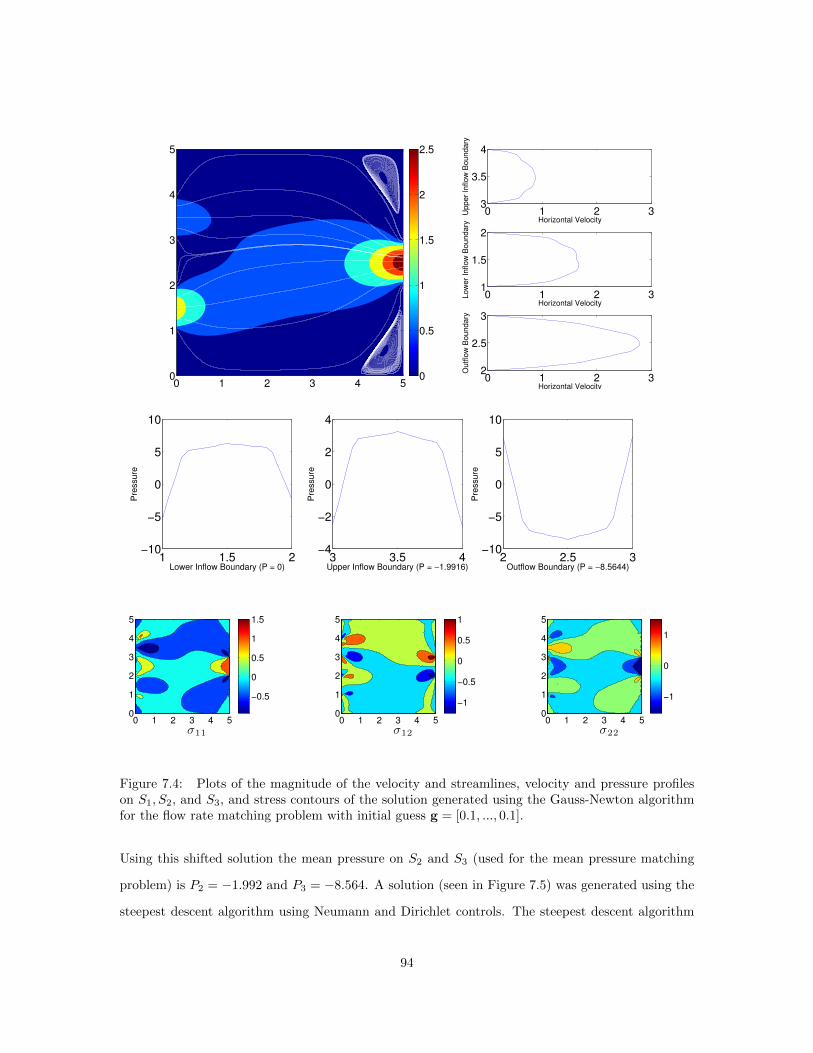
0 1 2 3 4 50
1
2
3
4
5
0
0.5
1
1.5
2
2.5
0 1 2 31
1.5
2
Horizontal Velocity
Low
er
Inflow
Boundary
0 1 2 33
3.5
4
Horizontal Velocity
Upper
Inflow
Boundary
0 1 2 32
2.5
3
Horizontal Velocity
Outflo
w B
oundary
1 1.5 2−10
−5
0
5
10
Pre
ssu
re
Lower Inflow Boundary (P = 0)3 3.5 4
−4
−2
0
2
4
Pre
ssu
re
Upper Inflow Boundary (P = −1.9916)2 2.5 3
−10
−5
0
5
10
Pre
ssu
re
Outflow Boundary (P = −8.5644)
σ11
0 1 2 3 4 50
1
2
3
4
5
−0.5
0
0.5
1
1.5
σ12
0 1 2 3 4 50
1
2
3
4
5
−1
−0.5
0
0.5
1
σ22
0 1 2 3 4 50
1
2
3
4
5
−1
0
1
Figure 7.4: Plots of the magnitude of the velocity and streamlines, velocity and pressure profileson S1, S2, and S3, and stress contours of the solution generated using the Gauss-Newton algorithmfor the flow rate matching problem with initial guess g = [0.1, ..., 0.1].
Using this shifted solution the mean pressure on S2 and S3 (used for the mean pressure matching
problem) is P2 = −1.992 and P3 = −8.564. A solution (seen in Figure 7.5) was generated using the
steepest descent algorithm using Neumann and Dirichlet controls. The steepest descent algorithm
94

converged in four iterations on both meshes. We observe from Figure 7.5 that the velocity stream-
lines generally agree with those found using Dirichlet boundary conditions and flow rate matching,
but there are significant differences in the speed contours, inlet/outlet velocity and pressure profiles,
as well as in the σ12 stress component at the inlets and outlet.
7.6.3 Further flow rate boundary conditions algorithm verification
As further verification of our steepest descent and Gauss-Newton algorithms for flow rate
matching, we consider again both algorithms, but now with the constant vector g = [5, ..., 5] as
an initial guess for both controls. Both algorithms converged, with the steepest descent needing
17 iterations while the Gauss-Newton algorithm converged in three iterations. The solutions are
displayed in Figures 7.6-7.7, respectively, and we observe they match each other exactly, but are
quite different from the solutions found with initial guess g = [0.1, ..., 0.1]. These and previous
results indicate that both algorithms converge to a same local minimum and the local minimum
found by the algorithms is determined by an initial guess.
95

0 1 2 3 4 50
1
2
3
4
5
0
0.5
1
1.5
2
2.5
0 1 2 31
1.5
2
Horizontal Velocity
Low
er
Inflow
Boundary
0 1 2 33
3.5
4
Horizontal Velocity
Upper
Inflow
Boundary
0 1 2 32
2.5
3
Horizontal Velocity
Outflo
w B
oundary
1 1.5 2−15
−10
−5
0
5
Pre
ssu
re
Lower Inflow Boundary (P = 0)3 3.5 4
−8
−6
−4
−2
0
2
Pre
ssu
re
Upper Inflow Boundary (P = −1.9916)2 2.5 3
−15
−10
−5
0
5
10P
ressu
re
Outflow Boundary (P = −8.5644)
σ11
0 1 2 3 4 50
1
2
3
4
5
−0.5
0
0.5
1
σ12
0 1 2 3 4 50
1
2
3
4
5
−1
−0.5
0
0.5
1
σ22
0 1 2 3 4 50
1
2
3
4
5
−1
−0.5
0
0.5
1
1.5
Figure 7.5: Plots of the magnitude of the velocity and streamlines, velocity and pressure profileson S1, S2, and S3, and stress contours of the solution generated using the steepest descent algorithmfor the mean pressure matching problem with initial guess g = [0.1, ..., 0.1].
96

0 1 2 3 4 50
1
2
3
4
5
0
0.5
1
1.5
2
2.5
3
0 1 2 31
1.5
2
Horizontal Velocity
Low
er
Inflow
Boundary
0 1 2 33
3.5
4
Horizontal Velocity
Upper
Inflow
Boundary
0 1 2 32
2.5
3
Horizontal Velocity
Outflo
w B
oundary
1 1.5 2−10
0
10
20
Pre
ssu
re
Lower Inflow Boundary (P = 0)3 3.5 4
−10
−5
0
5
10
15
Pre
ssu
re
Upper Inflow Boundary (P = −1.9916)2 2.5 3
−10
0
10
20P
ressu
re
Outflow Boundary (P = −8.5644)
σ11
0 1 2 3 4 50
1
2
3
4
5
−1
0
1
2
3
4
σ12
0 1 2 3 4 50
1
2
3
4
5
−2
0
2
4
σ22
0 1 2 3 4 50
1
2
3
4
5
0
2
4
Figure 7.6: Plots of the magnitude of the velocity and streamlines, velocity and pressure profileson S1, S2, and S3, and stress contours of the solution generated using the steepest descent algorithmfor the flow rate matching problem with initial guess g = [5, ..., 5].
97
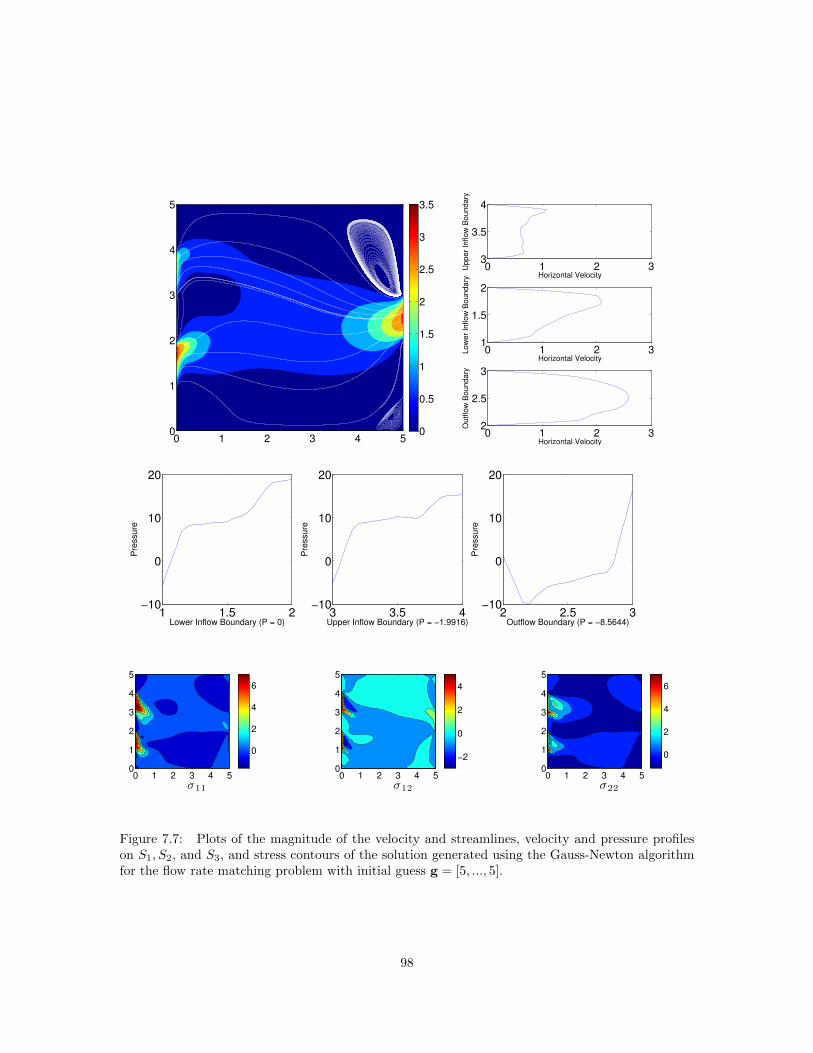
0 1 2 3 4 50
1
2
3
4
5
0
0.5
1
1.5
2
2.5
3
3.5
0 1 2 31
1.5
2
Horizontal Velocity
Low
er
Inflow
Boundary
0 1 2 33
3.5
4
Horizontal Velocity
Upper
Inflow
Boundary
0 1 2 32
2.5
3
Horizontal Velocity
Outflo
w B
oundary
1 1.5 2−10
0
10
20
Pre
ssu
re
Lower Inflow Boundary (P = 0)3 3.5 4
−10
0
10
20
Pre
ssu
re
Upper Inflow Boundary (P = −1.9916)2 2.5 3
−10
0
10
20P
ressu
re
Outflow Boundary (P = −8.5644)
σ11
0 1 2 3 4 50
1
2
3
4
5
0
2
4
6
σ12
0 1 2 3 4 50
1
2
3
4
5
−2
0
2
4
σ22
0 1 2 3 4 50
1
2
3
4
5
0
2
4
6
Figure 7.7: Plots of the magnitude of the velocity and streamlines, velocity and pressure profileson S1, S2, and S3, and stress contours of the solution generated using the Gauss-Newton algorithmfor the flow rate matching problem with initial guess g = [5, ..., 5].
98
Chapter 8
Conclusions
This work began in Chapter 3 where we studied a finite element method for the time-
dependent NSE based on the recently developed VVH formulation. Through a rigorous stability
analysis we have shown that the velocity is unconditionally stable, as is the vorticity if we penalize
the discrete solution to be ‘close’, in some sense, to the curl of the discrete velocity. Numerical
experiments show mixed results: for an idealized problem, optimal convergence rates are recovered
for the velocity and near-optimal convergence rates are recovered for the vorticity. However, on
channel flow problems over a step, it is clear that improved vorticity boundary conditions need to
be developed in order for this method to be competitive when higher order elements are used. In
Chapter 4 we addressed this problem by proposing a new, simple vorticity boundary condition. This
boundary condition, intended for portions of the domain where no-slip velocity boundary conditions
are to be enforced, was derived directly from the vorticity equation, and consisted of boundary
integrals of the pressure and forcing function. A 3d finite element method was then presented to
solve the steady NSE and vorticity equations implementing our new vorticity boundary conditions.
On a simple 3d problem, we verified that optimal convergence rates are achieved for the velocity
and vorticity solutions, and we are currently working on performing several 3d benchmark problems
to further test the method.
Chapter 5 derived a new, reduced order MDM, based off of the original MDM proposed
in [22]. The RMDM allowed us to derive a C0 finite element method that is unconditionally sta-
ble. Additionally, the method consists of a linearized backward Euler timestepping scheme which
decouples the filter solve, making the method efficient. We then proved analytically that optimal
99

convergence rates are achieved (with respect to the model solution). The chapter ended by imple-
menting our method on two benchmark 2d flow problems. In both examples, more accurate solutions
are recovered from the RMDM when we use two different spatial scales for the filters, verifying the
effectiveness of our multiscale model.
Our study of the defective boundary problem for non-Newtonian flows began in Chapter
6, where we considered a numerical method for generalized-Newtonian flows governed by the Cross
model with flow rate boundary conditions. The problem was formulated as a constrained optimal
control problem for which we proved solutions must exist. We then proved the existence of Lagrange
multipliers, and used the Lagrange multiplier method to derive an optimality system. Finally, a
steepest descent method was proposed that decouples the optimality system. We ended the chapter
by studying a complex 2d flow problem for which we were able to accurately and efficiently produce
solutions, verifying the robustness of our numerical method.
Chapter 7 investigated two numerical methods for viscoelastic flows with flow rate or mean
pressure boundary conditions. As in Chapter 6, the defective boundary problem was transformed
into an optimal control problem. The first method to solve this system stems from that presented
in Chapter 6, where an optimality system is derived using the Lagrange multiplier method, and a
steepest descent method is used to decouple and solve the optimality system. The second method
reconsidered the optimality system from a nonlinear least squares (NLS) viewpoint. We solved the
NLS problem by solving a related linear least squares problem (which was done using a conjugate
gradient method). Finally, a numerical experiment was considered to compare and contrast the two
methods, showing that the former is more robust, but the latter is more efficient.
100

Appendices
101

Appendix A deal.II code for 3d vorticity equation
1 /∗ ∗∗∗∗∗∗∗∗∗∗∗∗∗∗∗∗∗∗∗∗∗∗∗∗∗∗∗∗∗∗∗∗∗∗∗∗∗∗∗∗∗∗∗∗∗∗∗∗∗∗∗∗∗ ∗/
2 /∗ Author − Keith Galvin ∗/
3 /∗ Last updated − 6/4/13 ∗/
4 /∗ Model − 3d s te ady NSE and v o r t i c i t y equat ion ∗/
5 /∗ V e l o c i t y boundary c o n d i t i o n s : D i r i c h l e t ∗/
6 /∗ V o r t i c i t y boundary c o n d i t i o n s : New Natural v o r t bc ∗/
7 /∗ Nonlinear Method f o r s t ea dy NSE: Newton ’ s Method ∗/
8 /∗ S o l v e r − UMFPACK Sparse Direc t S o l v e r ∗/
9 /∗ ∗∗∗∗∗∗∗∗∗∗∗∗∗∗∗∗∗∗∗∗∗∗∗∗∗∗∗∗∗∗∗∗∗∗∗∗∗∗∗∗∗∗∗∗∗∗∗∗∗∗∗∗∗ ∗/
10
11 // Header F i l e s
12 #include <dea l . I I / base / t imer . h>
13 #include <dea l . I I / base / thread management . h>
14 #include <dea l . I I / base / m u l t i t h r e a d i n f o . h>
15 #include <dea l . I I / g r id / t r i a . h>
16 #include <dea l . I I / g r id / g r i d g e n e r a t o r . h>
17 #include <dea l . I I / g r id / t r i a a c c e s s o r . h>
18 #include <dea l . I I / g r id / t r i a i t e r a t o r . h>
19 #include <dea l . I I / g r id / g r i d t o o l s . h>
20 #include <dea l . I I / g r id / g r i d r e f i n e m e n t . h>
21 #include <dea l . I I / g r id / g r i d o u t . h>
22 #include <dea l . I I / do f s / do f hand l e r . h>
23 #include <dea l . I I / do f s / d o f t o o l s . h>
24 #include <dea l . I I / do f s / d o f a c c e s s o r . h>
25 #include <dea l . I I / do f s / dof renumber ing . h>
26 #include <dea l . I I / f e / f e q . h>
27 #include <dea l . I I / f e / f e v a l u e s . h>
28 #include <dea l . I I / f e / f e sy s t em . h>
29 #include <dea l . I I / base / q u a d r a t u r e l i b . h>
102

30 #include <dea l . I I / base / func t i on . h>
31 #include <dea l . I I / base / logstream . h>
32 #include <dea l . I I / base / u t i l i t i e s . h>
33 #include <dea l . I I / base / t e n s o r f u n c t i o n . h>
34 #include <dea l . I I / numerics / v e c t o r s . h>
35 #include <dea l . I I / numerics / matr i ce s . h>
36 #include <dea l . I I / numerics / data out . h>
37 #include <dea l . I I / numerics / e r r o r e s t i m a t o r . h>
38 #include <dea l . I I / l a c / f u l l m a t r i x . h>
39 #include <dea l . I I / l a c / s o l v e r c g . h>
40 #include <dea l . I I / l a c / pr e cond i t i on . h>
41 #include <dea l . I I / l a c / c o n s t r a i n t m a t r i x . h>
42 #include <dea l . I I / l a c / s p a r s e d i r e c t . h>
43 #include <dea l . I I / l a c / m a t r i x l i b . h>
44 #include <fstream>
45 #include <iostream>
46 #include <sstream>
47
48 using namespace d e a l i i ;
49
50 const long double pi = 3.141592653589793238462643;
51
52 /∗ ∗∗∗∗∗∗∗∗∗∗∗∗∗∗∗∗∗∗∗∗∗∗∗∗∗∗∗∗∗∗∗∗∗∗∗∗∗∗ ∗/
53 /∗ ∗/
54 /∗ Exact s o l u t i o n c l a s s implementat ions ∗/
55 /∗ ∗/
56 /∗ ∗∗∗∗∗∗∗∗∗∗∗∗∗∗∗∗∗∗∗∗∗∗∗∗∗∗∗∗∗∗∗∗∗∗∗∗∗∗ ∗/
57 /∗ ∗∗∗∗∗∗∗∗∗∗∗∗∗∗∗∗∗∗∗∗∗∗∗∗∗∗∗∗∗∗∗∗∗∗∗ ∗/
58 /∗ Exact s o l u t i o n c l a s s − v e l o c i t y ∗/
59 /∗ ∗∗∗∗∗∗∗∗∗∗∗∗∗∗∗∗∗∗∗∗∗∗∗∗∗∗∗∗∗∗∗∗∗∗∗ ∗/
103

60 template <int dim>
61 class ExactSo lut ion : public Function<dim>
62
63 public :
64 ExactSo lut ion ( ) : Function<dim> ( dim+1)
65
66 virtual double value ( const Point<dim> &p , const unsigned int
component ) const ;
67 virtual void v e c t o r v a l u e ( const Point<dim> &p , Vector<double> &
values ) const ;
68 virtual Tensor<1,dim> grad i en t ( const Point<dim> &p , const unsigned
int component ) const ;
69 virtual void v e c t o r g r a d i e n t ( const Point<dim> &p , std : : vector<Tensor
<1,dim> > &g r a d i e n t s ) const ;
70 ;
71
72 template <int dim>
73 double ExactSolut ion<dim> : : va lue ( const Point<dim> &p , const unsigned
int component ) const
74
75 i f ( component == 0)
76 return std : : s i n (2∗ pi ∗p [ 1 ] ) ;
77 else i f ( component == 1)
78 return std : : cos (2∗ pi ∗p [ 2 ] ) ;
79 else i f ( component == 2)
80 return std : : exp (p [ 0 ] ) ;
81 else i f ( component == 3)
82 return std : : s i n (2∗ pi ∗p [ 0 ] ) + cos (2∗ pi ∗p [ 1 ] ) + s i n (2∗ pi ∗p [ 2 ] ) ;
83
84 return 0 ;
104

85
86
87 template <int dim>
88 void ExactSolut ion<dim> : : v e c t o r v a l u e ( const Point<dim> &p , Vector<
double> &va lues ) const
89
90 for (unsigned int c =0; c<this−>n components ; c++)
91 va lue s ( c ) = ExactSolut ion<dim> : : va lue (p , c ) ;
92
93
94 template <int dim>
95 Tensor<1,dim> ExactSolut ion<dim> : : g rad i en t ( const Point<dim> &p , const
unsigned int component ) const
96
97 Tensor<1,dim> r e t u r n v a l u e ;
98
99 i f ( component == 0)
100
101 r e t u r n v a l u e [ 0 ] = 0 ;
102 r e t u r n v a l u e [ 1 ] = 2∗ pi ∗ std : : cos (2∗ pi ∗p [ 1 ] ) ;
103 r e t u r n v a l u e [ 2 ] = 0 ;
104
105 else i f ( component == 1)
106
107 r e t u r n v a l u e [ 0 ] = 0 ;
108 r e t u r n v a l u e [ 1 ] = 0 ;
109 r e t u r n v a l u e [ 2 ] = −2∗pi ∗ std : : s i n (2∗ pi ∗p [ 2 ] ) ;
110
111 else i f ( component == 2)
112
105

113 r e t u r n v a l u e [ 0 ] = std : : exp (p [ 0 ] ) ;
114 r e t u r n v a l u e [ 1 ] = 0 ;
115 r e t u r n v a l u e [ 2 ] = 0 ;
116
117 else
118
119 r e t u r n v a l u e [ 0 ] = 2∗ pi ∗ std : : cos (2∗ pi ∗p [ 0 ] ) ;
120 r e t u r n v a l u e [ 1 ] = −2∗pi ∗ std : : s i n (2∗ pi ∗p [ 1 ] ) ;
121 r e t u r n v a l u e [ 2 ] = 2∗ pi ∗ std : : cos (2∗ pi ∗p [ 2 ] ) ;
122
123
124 return r e t u r n v a l u e ;
125
126
127 template <int dim>
128 void ExactSolut ion<dim> : : v e c t o r g r a d i e n t ( const Point<dim> &p , std : :
vector<Tensor<1,dim> > &g r a d i e n t s ) const
129
130 for (unsigned int c =0; c<this−>n components ; c++)
131 g r a d i e n t s [ c ] = ExactSolut ion<dim> : : g rad i en t (p , c ) ;
132
133
134 /∗ ∗∗∗∗∗∗∗∗∗∗∗∗∗∗∗∗∗∗∗∗∗∗∗∗∗∗∗∗∗∗∗∗∗∗∗∗ ∗/
135 /∗ Exact s o l u t i o n c l a s s − v o r t i c i t y ∗/
136 /∗ ∗∗∗∗∗∗∗∗∗∗∗∗∗∗∗∗∗∗∗∗∗∗∗∗∗∗∗∗∗∗∗∗∗∗∗∗ ∗/
137 template <int dim>
138 class Exac tSo lu t i onVor t i c i t y : public Function<dim>
139
140 public :
141 Exac tSo lu t i onVor t i c i t y ( ) : Function<dim> ( dim )
106
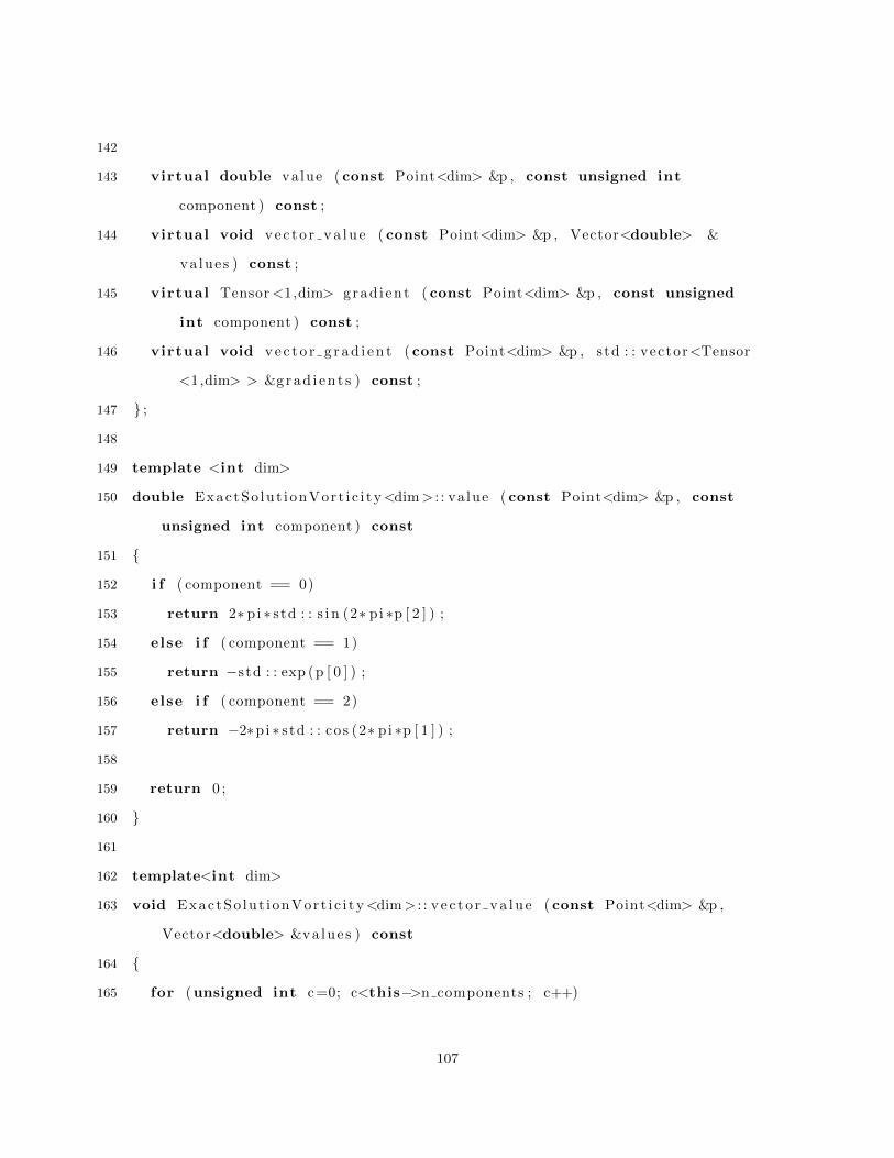
142
143 virtual double value ( const Point<dim> &p , const unsigned int
component ) const ;
144 virtual void v e c t o r v a l u e ( const Point<dim> &p , Vector<double> &
values ) const ;
145 virtual Tensor<1,dim> grad i en t ( const Point<dim> &p , const unsigned
int component ) const ;
146 virtual void v e c t o r g r a d i e n t ( const Point<dim> &p , std : : vector<Tensor
<1,dim> > &g r a d i e n t s ) const ;
147 ;
148
149 template <int dim>
150 double ExactSo lut i onVor t i c i ty<dim> : : va lue ( const Point<dim> &p , const
unsigned int component ) const
151
152 i f ( component == 0)
153 return 2∗ pi ∗ std : : s i n (2∗ pi ∗p [ 2 ] ) ;
154 else i f ( component == 1)
155 return −std : : exp (p [ 0 ] ) ;
156 else i f ( component == 2)
157 return −2∗pi ∗ std : : cos (2∗ pi ∗p [ 1 ] ) ;
158
159 return 0 ;
160
161
162 template<int dim>
163 void ExactSo lut i onVor t i c i ty<dim> : : v e c t o r v a l u e ( const Point<dim> &p ,
Vector<double> &va lues ) const
164
165 for (unsigned int c =0; c<this−>n components ; c++)
107
166 va lue s ( c ) = ExactSo lut i onVort i c i ty<dim> : : va lue (p , c ) ;
167
168
169 template <int dim>
170 Tensor<1,dim> ExactSo lut i onVor t i c i ty<dim> : : g rad i en t ( const Point<dim>
&p , const unsigned int component ) const
171
172 Tensor<1,dim> r e t u r n v a l u e ;
173
174 i f ( component == 0)
175
176 r e t u r n v a l u e [ 0 ] = 0 ;
177 r e t u r n v a l u e [ 1 ] = 0 ;
178 r e t u r n v a l u e [ 2 ] = 4∗ pi ∗ pi ∗ std : : cos (2∗ pi ∗p [ 2 ] ) ;
179
180 else i f ( component == 1)
181
182 r e t u r n v a l u e [ 0 ] = −std : : exp (p [ 0 ] ) ;
183 r e t u r n v a l u e [ 1 ] = 0 ;
184 r e t u r n v a l u e [ 2 ] = 0 ;
185
186 else i f ( component == 2)
187
188 r e t u r n v a l u e [ 0 ] = 0 ;
189 r e t u r n v a l u e [ 1 ] = 4∗ pi ∗ pi ∗ std : : s i n (2∗ pi ∗p [ 1 ] ) ;
190 r e t u r n v a l u e [ 2 ] = 0 ;
191
192
193 return r e t u r n v a l u e ;
194
108

195
196 template <int dim>
197 void ExactSo lut i onVor t i c i ty<dim> : : v e c t o r g r a d i e n t ( const Point<dim> &p ,
std : : vector<Tensor<1,dim> > &g r a d i e n t s ) const
198
199 for (unsigned int c =0; c<this−>n components ; c++)
200 g r a d i e n t s [ c ] = ExactSo lut i onVort i c i ty<dim> : : g rad i en t (p , c ) ;
201
202
203 /∗ ∗∗∗∗∗∗∗∗∗∗∗∗∗∗∗∗∗∗∗∗∗∗∗∗∗∗∗∗∗∗∗∗∗∗∗∗∗∗∗∗∗∗∗ ∗/
204 /∗ Exact s o l u t i o n c l a s s ( t e n s o r ) − v e l o c i t y ∗/
205 /∗ ∗∗∗∗∗∗∗∗∗∗∗∗∗∗∗∗∗∗∗∗∗∗∗∗∗∗∗∗∗∗∗∗∗∗∗∗∗∗∗∗∗∗∗ ∗/
206 template <int dim>
207 class ExactSolut ionTensor : public TensorFunction<1,dim>
208
209 public :
210 ExactSolut ionTensor ( ) : TensorFunction<1,dim>()
211 virtual Tensor<1,dim> value ( const Point<dim> &p) const ;
212 virtual void v a l u e l i s t ( const std : : vector<Point<dim> > &points , s td : :
vector<Tensor<1,dim> > &va lues ) const ;
213 virtual Tensor<2,dim> grad i ent ( const Point<dim> &p) const ;
214 virtual void g r a d i e n t l i s t ( const std : : vector<Point<dim> > &points ,
s td : : vector<Tensor<2,dim> > &va lues ) const ;
215 ;
216
217 template <int dim>
218 Tensor<1,dim> ExactSolut ionTensor<dim> : : va lue ( const Point<dim> &p)
const
219
220 ExactSolut ion<dim> utrue ;
109

221 Tensor<1,dim> ten ;
222
223 for (unsigned int d=0; d<dim ; d++)
224 ten [ d ] = utrue . va lue (p , d) ;
225
226 return ten ;
227
228
229 template <int dim>
230 void ExactSolut ionTensor<dim> : : v a l u e l i s t ( const std : : vector<Point<dim>
> &points , s td : : vector<Tensor<1,dim> > &va lues ) const
231
232 for (unsigned int p=0; p<po in t s . s i z e ( ) ; p++)
233
234 va lue s [ p ] . c l e a r ( ) ;
235 va lue s [ p ] = ExactSolutionTensor<dim> : : va lue ( po in t s [ p ] ) ;
236
237
238
239 template <int dim>
240 Tensor<2,dim> ExactSolut ionTensor<dim> : : g rad i en t ( const Point<dim> &p)
const
241
242 ExactSolut ion<dim> utrue ;
243 Tensor<2,dim> ten ;
244
245 for (unsigned int d=0; d<dim ; d++)
246 for (unsigned int c =0; c<dim ; c++)
247 ten [ d ] [ c ] = utrue . g rad i en t (p , d) [ c ] ;
248
110

249 return ten ;
250
251
252 template <int dim>
253 void ExactSolut ionTensor<dim> : : g r a d i e n t l i s t ( const std : : vector<Point<
dim> > &points , s td : : vector<Tensor<2,dim> > &va lues ) const
254
255 for (unsigned int p=0; p<po in t s . s i z e ( ) ; p++)
256
257 va lue s [ p ] . c l e a r ( ) ;
258 va lue s [ p ] = ExactSolutionTensor<dim> : : g rad i en t ( po in t s [ p ] ) ;
259
260
261
262 /∗ ∗∗∗∗∗∗∗∗∗∗∗∗∗∗∗∗∗∗∗∗∗∗∗∗∗∗∗∗∗∗∗∗∗∗∗∗∗∗∗∗∗∗∗∗ ∗/
263 /∗ Exact s o l u t i o n c l a s s ( t e n s o r ) − v o r t i c i t y ∗/
264 /∗ ∗∗∗∗∗∗∗∗∗∗∗∗∗∗∗∗∗∗∗∗∗∗∗∗∗∗∗∗∗∗∗∗∗∗∗∗∗∗∗∗∗∗∗∗ ∗/
265 template <int dim>
266 class ExactSo lut ionVort i c i tyTensor : public TensorFunction<1,dim>
267
268 public :
269 ExactSo lut ionVort i c i tyTensor ( ) : TensorFunction<1,dim>()
270 virtual Tensor<1,dim> value ( const Point<dim> &p) const ;
271 virtual void v a l u e l i s t ( const std : : vector<Point<dim> > &points , s td : :
vector<Tensor<1,dim> > &va lues ) const ;
272 ;
273
274 template <int dim>
275 Tensor<1,dim> ExactSo lut ionVort i c i tyTensor<dim> : : va lue ( const Point<dim>
&p) const
111
276
277 ExactSo lut i onVor t i c i ty<dim> c u r l u t r u e ;
278 Tensor<1,dim> ten ;
279
280 for (unsigned int d=0; d<dim ; d++)
281 ten [ d ] = c u r l u t r u e . va lue (p , d) ;
282
283 return ten ;
284
285
286 template <int dim>
287 void ExactSo lut ionVort i c i tyTensor<dim> : : v a l u e l i s t ( const std : : vector<
Point<dim> > &points , s td : : vector<Tensor<1,dim> > &va lues ) const
288
289 for (unsigned int p=0; p<po in t s . s i z e ( ) ; p++)
290
291 va lue s [ p ] . c l e a r ( ) ;
292 va lue s [ p ] = ExactSo lut ionVort i c i tyTensor<dim> : : va lue ( po in t s [ p ] ) ;
293
294
295
296
297 /∗ ∗∗∗∗∗∗∗∗∗∗∗∗∗∗∗∗∗∗∗∗∗∗∗∗∗∗∗ ∗/
298 /∗ ∗/
299 /∗ RHS c l a s s implementat ions ∗/
300 /∗ ∗/
301 /∗ ∗∗∗∗∗∗∗∗∗∗∗∗∗∗∗∗∗∗∗∗∗∗∗∗∗∗∗ ∗/
302 /∗ ∗∗∗∗∗∗∗∗∗∗∗∗∗∗∗∗∗∗∗∗∗∗∗∗∗∗∗∗∗∗∗∗ ∗/
303 /∗ RHS f u n c t i o n c l a s s − v e l o c i t y ∗/
304 /∗ ∗∗∗∗∗∗∗∗∗∗∗∗∗∗∗∗∗∗∗∗∗∗∗∗∗∗∗∗∗∗∗∗ ∗/
112

305 template <int dim>
306 class RightHandSide : public Function<dim>
307
308 public :
309 RightHandSide ( const double Reynolds ) : Function<dim> ( dim+1) , Reynolds
( Reynolds ) ;
310 virtual double value ( const Point<dim> &p , const unsigned int component
) const ;
311 virtual void v e c t o r v a l u e ( const Point<dim> &p , Vector<double> &va lues )
const ;
312 virtual void v e c t o r v a l u e l i s t ( const std : : vector<Point<dim> > &points ,
s td : : vector<Vector<double> > &v a l u e l i s t ) const ;
313 private :
314 const double Reynolds ;
315 ;
316
317 template <int dim>
318 double RightHandSide<dim> : : va lue ( const Point<dim> &p , const unsigned
int component ) const
319
320 const ExactSolut ionTensor<dim> uten ;
321 const ExactSolut ion<dim> u ;
322
323 i f ( component == 0)
324 return 2∗ pi ∗ std : : cos (2∗ pi ∗p [ 1 ] ) ∗ std : : cos (2∗ pi ∗p [ 2 ] ) + ( 1 . 0 / Reynolds )
∗4∗ pi ∗ pi ∗ std : : s i n (2∗ pi ∗p [ 1 ] ) + 2∗ pi ∗ std : : cos (2∗ pi ∗p [ 0 ] ) ;
325 else i f ( component == 1)
326 return −2∗pi ∗ std : : s i n (2∗ pi ∗p [ 2 ] ) ∗ std : : exp (p [ 0 ] ) + ( 1 . 0 / Reynolds ) ∗4∗
pi ∗ pi ∗ std : : cos (2∗ pi ∗p [ 2 ] ) − 2∗ pi ∗ std : : s i n (2∗ pi ∗p [ 1 ] ) ;
327 else i f ( component == 2)
113

328 return std : : s i n (2∗ pi ∗p [ 1 ] ) ∗ std : : exp (p [ 0 ] ) − ( 1 . 0 / Reynolds ) ∗ std : : exp (
p [ 0 ] ) + 2∗ pi ∗ std : : cos (2∗ pi ∗p [ 2 ] ) ;
329 else i f ( component == 3)
330 return 0 ;
331
332 return 0 ;
333
334
335 template <int dim>
336 void RightHandSide<dim> : : v e c t o r v a l u e ( const Point<dim> &p , Vector<double
> &va lues ) const
337
338 for (unsigned int c =0; c<this−>n components ; c++)
339 va lue s ( c ) = RightHandSide<dim> : : va lue (p , c ) ;
340
341
342 template <int dim>
343 void RightHandSide<dim> : : v e c t o r v a l u e l i s t ( const std : : vector<Point<dim>
> &points , s td : : vector<Vector<double> > &v a l u e l i s t ) const
344
345 const unsigned int n po in t s = po in t s . s i z e ( ) ;
346
347 for (unsigned int p=0; p<n po in t s ; p++)
348 RightHandSide<dim> : : v e c t o r v a l u e ( po in t s [ p ] , v a l u e l i s t [ p ] ) ;
349
350
351 /∗ ∗∗∗∗∗∗∗∗∗∗∗∗∗∗∗∗∗∗∗∗∗∗∗∗∗∗∗∗∗∗∗∗∗ ∗/
352 /∗ RHS f u n c t i o n c l a s s − v o r t i c i t y ∗/
353 /∗ ∗∗∗∗∗∗∗∗∗∗∗∗∗∗∗∗∗∗∗∗∗∗∗∗∗∗∗∗∗∗∗∗∗ ∗/
354 template <int dim>
114
355 class RightHandSideVort ic i ty : public Function<dim>
356
357 public :
358 RightHandSideVort ic i ty ( const double Reynolds ) : Function<dim> ( dim ) ,
Reynolds ( Reynolds ) ;
359 virtual double value ( const Point<dim> &p , const unsigned int component
) const ;
360 virtual void v e c t o r v a l u e ( const Point<dim> &p , Vector<double> &va lues )
const ;
361 virtual void v e c t o r v a l u e l i s t ( const std : : vector<Point<dim> > &points ,
s td : : vector<Vector<double> > &v a l u e l i s t ) const ;
362
363 private :
364 const double Reynolds ;
365 ;
366
367 template <int dim>
368 double RightHandSideVort ic ity<dim> : : va lue ( const Point<dim> &p , const
unsigned int component ) const
369
370 i f ( component == 0)
371 return 2∗ pi ∗ std : : cos (2∗ pi ∗p [ 1 ] ) ∗ std : : exp (p [ 0 ] ) + 4∗ pi ∗ pi ∗ std : : cos (2∗
pi ∗p [ 2 ] ) ∗ std : : exp (p [ 0 ] ) + ( 1 . 0 / Reynolds ) ∗8∗ pi ∗ pi ∗ pi ∗ std : : s i n (2∗
pi ∗p [ 2 ] ) ;
372 else i f ( component == 1)
373 return −4∗pi ∗ pi ∗ std : : s i n (2∗ pi ∗p [ 2 ] ) ∗ std : : cos (2∗ pi ∗p [ 1 ] ) − std : : s i n
(2∗ pi ∗p [ 1 ] ) ∗ std : : exp (p [ 0 ] ) + ( 1 . 0 / Reynolds ) ∗ std : : exp (p [ 0 ] ) ;
374 else i f ( component == 2)
375 return −2∗pi ∗ std : : s i n (2∗ pi ∗p [ 2 ] ) ∗ std : : exp (p [ 0 ] ) + 4∗ pi ∗ pi ∗ std : : cos
(2∗ pi ∗p [ 2 ] ) ∗ std : : s i n (2∗ pi ∗p [ 1 ] ) − ( 1 . 0 / Reynolds ) ∗8∗ pi ∗ pi ∗ pi ∗ std
115

: : cos (2∗ pi ∗p [ 1 ] ) ;
376
377 return 0 ;
378
379
380 template <int dim>
381 void RightHandSideVort ic ity<dim> : : v e c t o r v a l u e ( const Point<dim> &p ,
Vector<double> &va lues ) const
382
383 for (unsigned int c =0; c<this−>n components ; c++)
384 va lue s ( c ) = RightHandSideVort ic ity<dim> : : va lue (p , c ) ;
385
386
387 template <int dim>
388 void RightHandSideVort ic ity<dim> : : v e c t o r v a l u e l i s t ( const std : : vector<
Point<dim> > &points , s td : : vector<Vector<double> > &v a l u e l i s t )
const
389
390 const unsigned int n po in t s = po in t s . s i z e ( ) ;
391
392 for (unsigned int p=0; p<n po in t s ; p++)
393 RightHandSideVort ic ity<dim> : : v e c t o r v a l u e ( po in t s [ p ] , v a l u e l i s t [ p ] ) ;
394
395
396 /∗ ∗∗∗∗∗∗∗∗∗∗∗∗∗∗∗∗∗∗∗∗∗∗∗∗∗∗∗∗∗∗∗∗∗∗∗∗∗∗∗∗∗ ∗/
397 /∗ RHS f u n c t i o n c l a s s ( t e n s o r ) − v e l o c i t y ∗/
398 /∗ ∗∗∗∗∗∗∗∗∗∗∗∗∗∗∗∗∗∗∗∗∗∗∗∗∗∗∗∗∗∗∗∗∗∗∗∗∗∗∗∗∗ ∗/
399 template <int dim>
400 class RightHandSideTensor : public TensorFunction<1,dim>
401
116

402 public :
403 RightHandSideTensor ( const double Reynolds ) : TensorFunction<1,dim>() ,
Reynolds ( Reynolds )
404 virtual Tensor<1,dim> value ( const Point<dim> &p) const ;
405 virtual void v a l u e l i s t ( const std : : vector<Point<dim> > &points , s td : :
vector<Tensor<1,dim> > &va lues ) const ;
406
407 private :
408 const double Reynolds ;
409 ;
410
411 template <int dim>
412 Tensor<1,dim> RightHandSideTensor<dim> : : va lue ( const Point<dim> &p)
const
413
414 const RightHandSide<dim> rhs ( Reynolds ) ;
415 Tensor<1,dim> ten ;
416
417 for (unsigned int d=0; d<dim ; d++)
418 ten [ d ] = rhs . va lue (p , d) ;
419
420 return ten ;
421
422
423 template <int dim>
424 void RightHandSideTensor<dim> : : v a l u e l i s t ( const std : : vector<Point<dim>
> &points , s td : : vector<Tensor<1,dim> > &va lues ) const
425
426 for (unsigned int p=0; p<po in t s . s i z e ( ) ; p++)
427
117

428 va lue s [ p ] . c l e a r ( ) ;
429 va lue s [ p ] = RightHandSideTensor<dim> : : va lue ( po in t s [ p ] ) ;
430
431
432
433 /∗ ∗∗∗∗∗∗∗∗∗∗∗∗∗∗∗∗∗∗∗∗∗∗∗∗∗∗∗∗∗∗∗∗∗∗∗∗∗∗∗∗∗ ∗/
434 /∗ RHS f u n c t i o n c l a s s ( t e n s o r ) − v o r t i c i t y ∗/
435 /∗ ∗∗∗∗∗∗∗∗∗∗∗∗∗∗∗∗∗∗∗∗∗∗∗∗∗∗∗∗∗∗∗∗∗∗∗∗∗∗∗∗∗ ∗/
436 template <int dim>
437 class RightHandSideVort ic i tyTensor : public TensorFunction<1,dim>
438
439 public :
440 RightHandSideVort ic i tyTensor ( const double Reynolds ) : TensorFunction
<1,dim>() , Reynolds ( Reynolds )
441 virtual Tensor<1,dim> value ( const Point<dim> &p) const ;
442 virtual void v a l u e l i s t ( const std : : vector<Point<dim> > &points , s td : :
vector<Tensor<1,dim> > &va lues ) const ;
443
444 private :
445 const double Reynolds ;
446 ;
447
448 template <int dim>
449 Tensor<1,dim> RightHandSideVortic ityTensor<dim> : : va lue ( const Point<dim>
&p) const
450
451 const RightHandSideVort ic ity<dim> rhs ( Reynolds ) ;
452 Tensor<1,dim> ten ;
453
454 for (unsigned int d=0; d<dim ; d++)
118

455 ten [ d ] = rhs . va lue (p , d) ;
456
457 return ten ;
458
459
460 template <int dim>
461 void RightHandSideVort ic ityTensor<dim> : : v a l u e l i s t ( const std : : vector<
Point<dim> > &points , s td : : vector<Tensor<1,dim> > &va lues ) const
462
463 for (unsigned int p=0; p<po in t s . s i z e ( ) ; p++)
464
465 va lue s [ p ] . c l e a r ( ) ;
466 va lue s [ p ] = RightHandSideVortic ityTensor<dim> : : va lue ( po in t s [ p ] ) ;
467
468
469
470
471 /∗ ∗∗∗∗∗∗∗∗∗∗∗∗∗∗∗∗∗∗∗∗∗∗∗∗∗∗∗∗∗∗∗∗∗∗∗∗∗∗∗∗∗∗∗∗∗∗∗∗∗∗∗ ∗/
472 /∗ ∗/
473 /∗ D i r i c h l e t boundary f u n c t i o n c l a s s implementat ions ∗/
474 /∗ ∗/
475 /∗ ∗∗∗∗∗∗∗∗∗∗∗∗∗∗∗∗∗∗∗∗∗∗∗∗∗∗∗∗∗∗∗∗∗∗∗∗∗∗∗∗∗∗∗∗∗∗∗∗∗∗∗ ∗/
476 /∗ ∗∗∗∗∗∗∗∗∗∗∗∗∗∗∗∗∗∗∗∗∗∗∗∗∗∗∗∗∗∗∗∗∗∗∗∗∗∗ ∗/
477 /∗ Boundary f u n c t i o n c l a s s − v e l o c i t y ∗/
478 /∗ ∗∗∗∗∗∗∗∗∗∗∗∗∗∗∗∗∗∗∗∗∗∗∗∗∗∗∗∗∗∗∗∗∗∗∗∗∗∗ ∗/
479 template <int dim>
480 class BoundaryValues : public Function<dim>
481
482 public :
483 BoundaryValues ( ) : Function<dim> ( dim+1) ;
119

484 virtual double value ( const Point<dim> &p , const unsigned int
component ) const ;
485 virtual void v e c t o r v a l u e ( const Point<dim> &p , Vector<double> &value )
const ;
486 ;
487
488 template <int dim>
489 double BoundaryValues<dim> : : va lue ( const Point<dim> &p , const unsigned
int component ) const
490
491 const ExactSolut ion<dim> utrue ;
492 return utrue . va lue (p , component ) ;
493
494 return 0 ;
495
496
497 template <int dim>
498 void BoundaryValues<dim> : : v e c t o r v a l u e ( const Point<dim> &p , Vector<
double> &va lues ) const
499
500 for (unsigned int c =0; c < this−>n components ; c++)
501 va lue s ( c ) = BoundaryValues<dim> : : va lue (p , c ) ;
502
503
504 /∗ ∗∗∗∗∗∗∗∗∗∗∗∗∗∗∗∗∗∗∗∗∗∗∗∗∗∗∗∗∗∗∗∗∗∗∗∗∗∗ ∗/
505 /∗ Boundary f u n c t i o n c l a s s − v o r t i c i t y ∗/
506 /∗ ∗∗∗∗∗∗∗∗∗∗∗∗∗∗∗∗∗∗∗∗∗∗∗∗∗∗∗∗∗∗∗∗∗∗∗∗∗∗ ∗/
507 template <int dim>
508 class BoundaryValuesVort ic i ty : public Function<dim>
509
120
510 public :
511 BoundaryValuesVort ic i ty ( ) : Function<dim> ( dim) ;
512 virtual double value ( const Point<dim> &p , const unsigned int
component ) const ;
513 virtual void v e c t o r v a l u e ( const Point<dim> &p , Vector<double> &value )
const ;
514 ;
515
516 template <int dim>
517 double BoundaryValuesVortic ity<dim> : : va lue ( const Point<dim> &p , const
unsigned int component ) const
518
519 const ExactSo lut i onVor t i c i ty<dim> wtrue ;
520 return wtrue . va lue (p , component ) ;
521
522
523 return 0 ;
524
525
526 template <int dim>
527 void BoundaryValuesVort ic ity<dim> : : v e c t o r v a l u e ( const Point<dim> &p ,
Vector<double> &va lues ) const
528
529 for (unsigned int c =0; c < this−>n components ; c++)
530 va lue s ( c ) = BoundaryValuesVortic ity<dim> : : va lue (p , c ) ;
531
532
533 /∗ ∗∗∗∗∗∗∗∗∗∗∗∗∗∗∗∗∗∗∗∗∗∗∗∗∗∗∗∗∗∗∗∗∗∗∗∗∗∗∗∗∗∗∗∗∗∗ ∗/
534 /∗ Boundary f u n c t i o n c l a s s ( t e n s o r ) − v e l o c i t y ∗/
535 /∗ ∗∗∗∗∗∗∗∗∗∗∗∗∗∗∗∗∗∗∗∗∗∗∗∗∗∗∗∗∗∗∗∗∗∗∗∗∗∗∗∗∗∗∗∗∗∗ ∗/
121

536 template <int dim>
537 class BoundaryValuesTensor : public TensorFunction<1,dim>
538
539 public :
540 BoundaryValuesTensor ( ) : TensorFunction<1,dim>()
541 virtual Tensor<1,dim> value ( const Point<dim> &p) const ;
542 virtual void v a l u e l i s t ( const std : : vector<Point<dim> > &points , s td : :
vector<Tensor<1,dim> > &va lues ) const ;
543 ;
544
545 template <int dim>
546 Tensor<1,dim> BoundaryValuesTensor<dim> : : va lue ( const Point<dim> &p)
const
547
548 const BoundaryValues<dim> g ;
549 Tensor<1,dim> ten ;
550
551 for (unsigned int d=0; d<dim ; d++)
552 ten [ d ] = g . va lue (p , d) ;
553
554 return ten ;
555
556
557 template <int dim>
558 void BoundaryValuesTensor<dim> : : v a l u e l i s t ( const std : : vector<Point<dim>
> &points , s td : : vector<Tensor<1,dim> > &va lues ) const
559
560 for (unsigned int p=0; p<po in t s . s i z e ( ) ; p++)
561
562 va lue s [ p ] . c l e a r ( ) ;
122

563 va lue s [ p ] = BoundaryValuesTensor<dim> : : va lue ( po in t s [ p ] ) ;
564
565
566
567
568 /∗ ∗∗∗∗∗∗∗∗∗∗∗∗∗∗∗∗∗∗∗∗∗∗∗∗∗∗∗∗∗∗∗∗∗∗∗∗∗∗∗∗∗∗∗∗∗∗∗∗∗∗∗∗∗∗∗ ∗/
569 /∗ ∗/
570 /∗ Steady NSE / v o r t i c i t y equat ion c l a s s implementat ions ∗/
571 /∗ ∗/
572 /∗ ∗∗∗∗∗∗∗∗∗∗∗∗∗∗∗∗∗∗∗∗∗∗∗∗∗∗∗∗∗∗∗∗∗∗∗∗∗∗∗∗∗∗∗∗∗∗∗∗∗∗∗∗∗∗∗ ∗/
573 template <int dim>
574 class SNSE
575
576 public :
577 SNSE ( ) ;
578 ˜SNSE ( ) ;
579 void run ( ) ;
580
581 private :
582 void make grid ( ) ;
583 void setup system ( ) ;
584 void a s s em b l e v e l o c i t y s y s t e m ( ) ;
585 void a s s e m b l e v e l o c i t y s y s t e m i n t e r v a l ( const typename DoFHandler<dim
> : : a c t i v e c e l l i t e r a t o r &begin , const typename DoFHandler<dim> : :
a c t i v e c e l l i t e r a t o r &end ) ;
586 void a s s e m b l e v o r t i c i t y s y s t e m ( ) ;
587 void s o l v e v e l ( ) ;
588 void s o l v e v o r t ( ) ;
589 double compute re lat ive norm ( ) ;
590 void compute error ( ) ;
123

591 void o u t p u t r e s u l t s ( ) ;
592
593 std : : s t r i n g outpath ;
594 Threads : : Mutex a s s emb l e r l o ck ;
595
596 const unsigned int num mesh div ;
597 const unsigned int d e g r e e v e l ;
598 const unsigned int deg r e e vo r t ;
599 const double Re ;
600
601 Triangulat ion<dim> t r i a n g u l a t i o n ;
602
603 FESystem<dim> f e v e l ;
604 Constra intMatr ix c o n s t r a i n t s v e l ;
605 DoFHandler<dim> d o f h a n d l e r v e l ;
606 Spars i tyPat te rn s p a r s i t y p a t t e r n v e l ;
607 SparseMatrix<double> sy s t em matr ix ve l ;
608 Vector<double> s y s t e m r h s v e l ;
609 Vector<double> p r e v s o l u t i o n v e l ;
610
611 FESystem<dim> f e v o r t ;
612 Constra intMatr ix c o n s t r a i n t s v o r t ;
613 DoFHandler<dim> d o f h a n d l e r v o r t ;
614 Spars i tyPat te rn s p a r s i t y p a t t e r n v o r t ;
615 SparseMatrix<double> sys tem matr ix vor t ;
616 Vector<double> sy s t em rhs vo r t ;
617 ;
618
619
620 /∗ ∗∗∗∗∗∗∗∗∗∗∗∗∗∗∗∗∗∗∗∗∗∗∗∗∗∗∗∗∗∗ ∗/
124

621 /∗ Class c o n s t r u c t o r / d e s t r u c t o r ∗/
622 /∗ ∗∗∗∗∗∗∗∗∗∗∗∗∗∗∗∗∗∗∗∗∗∗∗∗∗∗∗∗∗∗ ∗/
623 template <int dim>
624 SNSE<dim> : :SNSE ( )
625 :
626 num mesh div (4 ) ,
627 d e g r e e v e l (2 ) ,
628 deg r e e vo r t (2 ) ,
629 Re ( 1 . 0 ) ,
630 f e v e l (FE Q<dim>( d e g r e e v e l ) , dim , FE Q<dim>( deg r e e ve l −1) ,1 ) ,
631 d o f h a n d l e r v e l ( t r i a n g u l a t i o n ) ,
632 f e v o r t (FE Q<dim>( deg r e e vo r t ) , dim ) ,
633 d o f h a n d l e r v o r t ( t r i a n g u l a t i o n )
634
635 outpath = ” Vort i c i tyEq ” ;
636
637
638 template <int dim>
639 SNSE<dim> : :˜SNSE ( )
640
641 d o f h a n d l e r v e l . c l e a r ( ) ;
642 d o f h a n d l e r v o r t . c l e a r ( ) ;
643
644
645
646 /∗ ∗∗∗∗∗∗∗∗∗∗∗∗∗∗∗∗∗∗∗ ∗/
647 /∗ Mesh Generation ∗/
648 /∗ ∗∗∗∗∗∗∗∗∗∗∗∗∗∗∗∗∗∗∗ ∗/
649 template <int dim>
650 void SNSE<dim> : : make grid ( )
125

651
652 std : : cout << ” Reynolds number i s : ” << Re << std : : endl ;
653 std : : cout << ” Construct ing the mesh . . . ” << std : : endl ;
654
655 GridGenerator : : subd iv ided hyper cube ( t r i a n g u l a t i o n , num mesh div , 0 ,
1) ;
656
657 std : : s t r i n g f i l ename = outpath+”Mesh . eps ” ;
658 std : : o f s tream output ( f i l ename . c s t r ( ) ) ;
659 GridOut g r i d o u t ;
660 g r i d o u t . w r i t e e p s ( t r i a n g u l a t i o n , output ) ;
661
662 for (typename Triangulat ion<dim> : : a c t i v e c e l l i t e r a t o r c e l l =
t r i a n g u l a t i o n . b e g i n a c t i v e ( ) ; c e l l != t r i a n g u l a t i o n . end ( ) ; ++c e l l )
663 for (unsigned int f =0; f<GeometryInfo<dim> : : f a c e s p e r c e l l ; ++f )
664
665 i f ( c e l l−>f a c e ( f )−>cente r ( ) [ dim−2] == 0 | | c e l l−>f a c e ( f )−>cente r
( ) [ dim−2] == 1)
666 c e l l−>f a c e ( f )−>s e t a l l b o u n d a r y i n d i c a t o r s (1 ) ;
667 i f ( c e l l−>f a c e ( f )−>cente r ( ) [ dim−1] == 0 | | c e l l−>f a c e ( f )−>cente r
( ) [ dim−1] == 1)
668 c e l l−>f a c e ( f )−>s e t a l l b o u n d a r y i n d i c a t o r s (2 ) ;
669
670
671
672
673 /∗ ∗∗∗∗∗∗∗∗∗∗∗∗∗∗∗∗ ∗/
674 /∗ System Setup ∗/
675 /∗ ∗∗∗∗∗∗∗∗∗∗∗∗∗∗∗∗ ∗/
676 template <int dim>
126

677 void SNSE<dim> : : se tup system ( )
678
679 std : : cout << ” I n i t i a l i z i n g . . . ” << std : : endl ;
680
681 // I n i t i a l i z e v e l o c i t y / p r e s s u r e
682 d o f h a n d l e r v e l . d i s t r i b u t e d o f s ( f e v e l ) ;
683
684 c o n s t r a i n t s v e l . c l e a r ( ) ;
685
686 std : : vector<bool> component mask vel ( dim+1, true ) ;
687 component mask vel [ dim ] = fa l se ;
688 VectorTools : : i n t e r p o l a t e b o u n d a r y v a l u e s ( d o f h a n d l e r v e l , 0 ,
BoundaryValues<dim>() , c o n s t r a i n t s v e l , component mask vel ) ;
689 VectorTools : : i n t e r p o l a t e b o u n d a r y v a l u e s ( d o f h a n d l e r v e l , 1 ,
BoundaryValues<dim>() , c o n s t r a i n t s v e l , component mask vel ) ;
690 VectorTools : : i n t e r p o l a t e b o u n d a r y v a l u e s ( d o f h a n d l e r v e l , 2 ,
BoundaryValues<dim>() , c o n s t r a i n t s v e l , component mask vel ) ;
691
692 std : : vector<bool> component mask pres ( dim+1, fa l se ) ;
693 component mask pres [ dim ] = true ;
694 std : : vector<bool> boundary dofs ( d o f h a n d l e r v e l . n do f s ( ) , fa l se ) ;
695 DoFTools : : ex t rac t boundary do f s ( d o f h a n d l e r v e l ,
component mask pres , boundary dofs ) ;
696
697 const unsigned int f i r s t b o u n d a r y d o f = std : : d i s t anc e ( boundary dofs
. begin ( ) , s td : : f i n d ( boundary dofs . begin ( ) , boundary dofs . end ( ) ,
true ) ) ;
698
699 c o n s t r a i n t s v e l . a d d l i n e ( f i r s t b o u n d a r y d o f ) ;
700 for (unsigned int i=f i r s t b o u n d a r y d o f +1; i<d o f h a n d l e r v e l . n do f s ( )
127

; ++i )
701 i f ( boundary dofs [ i ] == true )
702 c o n s t r a i n t s v e l . add entry ( f i r s t b o u n d a r y d o f , i , −1) ;
703
704 c o n s t r a i n t s v e l . c l o s e ( ) ;
705
706 CompressedSpars ityPattern c s p v e l ( d o f h a n d l e r v e l . n do f s ( ) ) ;
707 DoFTools : : make spar s i ty pat t e rn ( d o f h a n d l e r v e l , c sp ve l ,
c o n s t r a i n t s v e l , fa l se ) ;
708 s p a r s i t y p a t t e r n v e l . copy from ( c s p v e l ) ;
709 sy s t em matr ix ve l . r e i n i t ( s p a r s i t y p a t t e r n v e l ) ;
710 s y s t e m r h s v e l . r e i n i t ( d o f h a n d l e r v e l . n do f s ( ) ) ;
711 p r e v s o l u t i o n v e l . r e i n i t ( d o f h a n d l e r v e l . n do f s ( ) ) ;
712
713 std : : cout << ”Number o f v e l o c i t y / p r e s su r e degree s o f freedom : ” <<
d o f h a n d l e r v e l . n do f s ( ) << std : : endl ;
714
715 // I n i t i a l i z e v o r t i c i t y
716 d o f h a n d l e r v o r t . d i s t r i b u t e d o f s ( f e v o r t ) ;
717
718 c o n s t r a i n t s v o r t . c l e a r ( ) ;
719
720 std : : vector<bool> component mask x (dim , fa l se ) ;
721 component mask x [ dim−3] = true ;
722 VectorTools : : i n t e r p o l a t e b o u n d a r y v a l u e s ( do f hand l e r vo r t , 0 ,
BoundaryValuesVortic ity<dim>() , c o n s t r a i n t s v o r t ,
component mask x ) ;
723 std : : vector<bool> component mask y (dim , fa l se ) ;
724 component mask y [ dim−2] = true ;
725 VectorTools : : i n t e r p o l a t e b o u n d a r y v a l u e s ( do f hand l e r vo r t , 1 ,
128

BoundaryValuesVortic ity<dim>() , c o n s t r a i n t s v o r t ,
component mask y ) ;
726 std : : vector<bool> component mask z (dim , fa l se ) ;
727 component mask z [ dim−1] = true ;
728 VectorTools : : i n t e r p o l a t e b o u n d a r y v a l u e s ( do f hand l e r vo r t , 2 ,
BoundaryValuesVortic ity<dim>() , c o n s t r a i n t s v o r t ,
component mask z ) ;
729
730 c o n s t r a i n t s v o r t . c l o s e ( ) ;
731
732 CompressedSpars ityPattern c sp vo r t ( d o f h a n d l e r v o r t . n do f s ( ) ) ;
733 DoFTools : : make spar s i ty pat t e rn ( do f hand l e r vo r t , c sp vort ,
c o n s t r a i n t s v o r t , fa l se ) ;
734 s p a r s i t y p a t t e r n v o r t . copy from ( c sp vo r t ) ;
735 sys tem matr ix vor t . r e i n i t ( s p a r s i t y p a t t e r n v o r t ) ;
736 sy s t em rhs vo r t . r e i n i t ( d o f h a n d l e r v o r t . n do f s ( ) ) ;
737
738 std : : cout << ”Number o f v o r t i c i t y degree s o f freedom : ” <<
d o f h a n d l e r v o r t . n do f s ( ) << std : : endl ;
739
740
741
742 /∗ ∗∗∗∗∗∗∗∗∗∗∗∗∗∗∗∗∗∗∗∗∗∗∗∗∗∗∗∗ ∗/
743 /∗ V e l o c i t y System Assembly ∗/
744 /∗ ∗∗∗∗∗∗∗∗∗∗∗∗∗∗∗∗∗∗∗∗∗∗∗∗∗∗∗∗ ∗/
745 template <int dim>
746 void SNSE<dim> : : a s s em b l e v e l o c i t y s y s t e m ( )
747
748 Timer AssemblyTimer ;
749 AssemblyTimer . s t a r t ( ) ;
129
750
751 const unsigned int n threads = m u l t i t h r e a d i n f o . n d e f a u l t t h r e a d s ;
752 std : : cout << ” Assembling the v e l o c i t y system matrix and rhs vec to r ( ”
<< n threads << ” threads assembl ing in p a r a l l e l ) . . . ” << std : : endl
;
753
754 sy s t em matr ix ve l = 0 ;
755 s y s t e m r h s v e l = 0 ;
756
757 Threads : : ThreadGroup<> threads ;
758
759 typedef typename DoFHandler<dim> : : a c t i v e c e l l i t e r a t o r
a c t i v e c e l l i t e r a t o r ;
760 std : : vector<std : : pa ir<a c t i v e c e l l i t e r a t o r , a c t i v e c e l l i t e r a t o r > >
th read ranges = Threads : : s p l i t r a n g e<a c t i v e c e l l i t e r a t o r > (
d o f h a n d l e r v e l . b e g i n a c t i v e ( ) , d o f h a n d l e r v e l . end ( ) , n threads
) ;
761
762 for (unsigned int thread =0; thread<n threads ; ++thread )
763 threads += Threads : : new thread (&SNSE<dim> : :
a s s e m b l e v e l o c i t y s y s t e m i n t e r v a l , ∗ this , th read ranges [ thread ] .
f i r s t , th read ranges [ thread ] . second ) ;
764
765 threads . j o i n a l l ( ) ;
766
767 AssemblyTimer . stop ( ) ;
768 std : : cout << ” Elapsed wal l time : ” << std : : f l o o r ( AssemblyTimer .
wa l l t ime ( ) + 0 . 5 ) << ” seconds ” << std : : endl ;
769
770
130
771
772 /∗ ∗∗∗∗∗∗∗∗∗∗∗∗∗∗∗∗∗∗∗∗∗∗∗∗∗∗∗∗∗∗∗∗∗∗∗∗ ∗/
773 /∗ V e l o c i t y System Assembly I n t e r v a l ∗/
774 /∗ ∗∗∗∗∗∗∗∗∗∗∗∗∗∗∗∗∗∗∗∗∗∗∗∗∗∗∗∗∗∗∗∗∗∗∗∗ ∗/
775 template <int dim>
776 void SNSE<dim> : : a s s e m b l e v e l o c i t y s y s t e m i n t e r v a l ( const typename
DoFHandler<dim> : : a c t i v e c e l l i t e r a t o r &begin , const typename
DoFHandler<dim> : : a c t i v e c e l l i t e r a t o r &end )
777
778 sy s t em matr ix ve l = 0 ;
779 s y s t e m r h s v e l = 0 ;
780
781 QGauss<dim> quadrature formula ( d e g r e e v e l + 1) ;
782 const unsigned int n q p o i n t s = quadrature formula . s i z e ( ) ;
783
784 FEValues<dim> f e v a l u e s ( f e v e l , quadrature formula , update va lues |
update g rad i ent s | update quadrature po int s | update JxW values ) ;
785 const unsigned int d o f s p e r c e l l = f e v e l . d o f s p e r c e l l ;
786 std : : vector<unsigned int> l o c a l d o f i n d i c e s ( d o f s p e r c e l l ) ;
787
788 const RightHandSide<dim> r i g h t h a n d s i d e (Re) ;
789
790 FullMatrix<double> c e l l m a t r i x ( d o f s p e r c e l l , d o f s p e r c e l l ) ;
791 Vector<double> c e l l r h s ( d o f s p e r c e l l ) ;
792
793 std : : vector<Vector<double> > r h s v a l u e s ( n q po int s , Vector<double>(dim
+1) ) ;
794 std : : vector<Tensor<1,dim> > p r e v v e l v a l u e s ( n q p o i n t s ) ;
795 std : : vector<Tensor<2,dim> > p r e v v e l g r a d s ( n q p o i n t s ) ;
796
131
797 std : : vector<Tensor<2,dim> > grad ph i u ( d o f s p e r c e l l ) ;
798 std : : vector<double> d iv ph i u ( d o f s p e r c e l l ) ;
799 std : : vector<Tensor<1,dim> > phi u ( d o f s p e r c e l l ) ;
800 std : : vector<double> phi p ( d o f s p e r c e l l ) ;
801
802 const FEValuesExtractors : : Vector v e l o c i t i e s (0 ) ;
803 const FEValuesExtractors : : S ca l a r p r e s su r e ( dim ) ;
804
805 typename DoFHandler<dim> : : a c t i v e c e l l i t e r a t o r c e l l ;
806
807 for ( c e l l = begin ; c e l l !=end ; c e l l ++)
808
809 f e v a l u e s . r e i n i t ( c e l l ) ;
810
811 c e l l m a t r i x = 0 ;
812 c e l l r h s = 0 ;
813
814 r i g h t h a n d s i d e . v e c t o r v a l u e l i s t ( f e v a l u e s . g e t q u a d r a t u r e p o i n t s
( ) , r h s v a l u e s ) ;
815 f e v a l u e s [ v e l o c i t i e s ] . g e t f u n c t i o n v a l u e s ( p r e v s o l u t i o n v e l ,
p r e v v e l v a l u e s ) ;
816 f e v a l u e s [ v e l o c i t i e s ] . g e t f u n c t i o n g r a d i e n t s ( p r e v s o l u t i o n v e l ,
p r e v v e l g r a d s ) ;
817
818 for (unsigned int q=0; q<n q p o i n t s ; q++)
819
820 for (unsigned int k=0; k<d o f s p e r c e l l ; k++)
821
822 grad ph i u [ k ] = f e v a l u e s [ v e l o c i t i e s ] . g rad i ent (k , q ) ;
823 d iv ph i u [ k ] = f e v a l u e s [ v e l o c i t i e s ] . d ive rgence (k , q ) ;
132

824 phi u [ k ] = f e v a l u e s [ v e l o c i t i e s ] . va lue (k , q ) ;
825 phi p [ k ] = f e v a l u e s [ p r e s su r e ] . va lue (k , q ) ;
826
827
828 for (unsigned int i =0; i<d o f s p e r c e l l ; i++)
829
830 for (unsigned int j =0; j<d o f s p e r c e l l ; j++)
831 c e l l m a t r i x ( i , j ) += ( grad ph i u [ j ]∗ p r e v v e l v a l u e s [ q ]∗
phi u [ i ]
832 + p r e v v e l g r a d s [ q ]∗ phi u [ j ]∗ phi u [
i ]
833 + ( 1 . 0 / Re) ∗ doub l e cont rac t (
grad ph i u [ j ] , g rad ph i u [ i ] )
834 − phi p [ j ]∗ d iv ph i u [ i ]
835 + div ph i u [ j ]∗ phi p [ i ]
836 ) ∗ f e v a l u e s .JxW( q ) ;
837
838 const unsigned int component i = f e v e l .
system to component index ( i ) . f i r s t ;
839 c e l l r h s ( i ) += ( f e v a l u e s . shape va lue ( i , q ) ∗ r h s v a l u e s [ q ] (
component i ) + p r e v v e l g r a d s [ q ]∗ p r e v v e l v a l u e s [ q ]∗
phi u [ i ] ) ∗ f e v a l u e s .JxW( q ) ;
840
841
842
843 c e l l−>g e t d o f i n d i c e s ( l o c a l d o f i n d i c e s ) ;
844
845 a s s emb l e r l o ck . a cqu i r e ( ) ;
846 c o n s t r a i n t s v e l . d i s t r i b u t e l o c a l t o g l o b a l ( c e l l m a t r i x , c e l l r h s ,
l o c a l d o f i n d i c e s , sys tem matr ix ve l , s y s t e m r h s v e l ) ;
133
847 a s s emb l e r l o ck . r e l e a s e ( ) ;
848
849
850
851
852 /∗ ∗∗∗∗∗∗∗∗∗∗∗∗∗∗∗∗∗∗∗∗∗∗∗∗∗∗∗∗∗ ∗/
853 /∗ V o r t i c i t y System Assembly ∗/
854 /∗ ∗∗∗∗∗∗∗∗∗∗∗∗∗∗∗∗∗∗∗∗∗∗∗∗∗∗∗∗∗ ∗/
855 template <int dim>
856 void SNSE<dim> : : a s s e m b l e v o r t i c i t y s y s t e m ( )
857
858 std : : cout << std : : endl << ” Assembling the v o r t i c i t y system matrix and
RHS vecto r . . . ” << std : : endl ;
859
860 Timer AssemblyTimer ;
861 AssemblyTimer . s t a r t ( ) ;
862
863 QGauss<dim> quadrature formula ( deg r e e vo r t + 1) ;
864 QGauss<dim−1> f a c e quadra tu r e f o rmu la ( deg r e e vo r t + 1) ;
865 const unsigned int n q p o i n t s = quadrature formula . s i z e ( ) ;
866 const unsigned int n f a c e q p o i n t s = face quadra tu r e f o rmu la . s i z e ( ) ;
867
868 FEValues<dim> f e v a l u e s v e l ( f e v e l , quadrature formula , update va lues
| update g rad i ent s | update quadrature po int s | update JxW values
) ;
869 FEValues<dim> f e v a l u e s v o r t ( f e v o r t , quadrature formula ,
update va lues | update g rad i ent s | update quadrature po int s |
update JxW values ) ;
870 FEFaceValues<dim> f e f a c e v a l u e s v e l ( f e v e l , f a ce quadrature fo rmula ,
update va lues | update g rad i ent s | update normal vector s |
134

update quadrature po int s | update JxW values ) ;
871 FEFaceValues<dim> f e f a c e v a l u e s v o r t ( f e v o r t ,
f a ce quadrature fo rmula , update va lues | update g rad i ent s |
update normal vector s | update quadrature po int s |
update JxW values ) ;
872
873 const unsigned int d o f s p e r c e l l = f e v o r t . d o f s p e r c e l l ;
874 std : : vector<unsigned int> l o c a l d o f i n d i c e s ( d o f s p e r c e l l ) ;
875
876 const RightHandSideVort ic ity<dim> r i g h t h a n d s i d e v o r t (Re) ;
877 const RightHandSideTensor<dim> r i g h t h a n d s i d e t e n s o r (Re) ;
878 const BoundaryValuesTensor<dim> g ;
879
880 FullMatrix<double> c e l l m a t r i x ( d o f s p e r c e l l , d o f s p e r c e l l ) ;
881 Vector<double> c e l l r h s ( d o f s p e r c e l l ) ;
882
883 std : : vector<Vector<double> > r h s v a l u e s ( n q po int s , Vector<double>(dim
) ) ;
884 std : : vector<Tensor<1,dim> > v e l o c i t y v a l u e s ( n q p o i n t s ) ;
885 std : : vector<Tensor<2,dim> > v e l o c i t y g r a d s ( n q p o i n t s ) ;
886 std : : vector<Tensor<1,dim> > r h s f a c e v a l u e s ( n f a c e q p o i n t s ) ;
887 std : : vector<Tensor<1,dim> > r h s f a c e f x n ( n f a c e q p o i n t s ) ;
888 std : : vector<Tensor<1,dim> > g va lu e s ( n f a c e q p o i n t s ) ;
889 std : : vector<Tensor<1,dim> > v e l o c i t y f a c e v a l u e s ( n f a c e q p o i n t s ) ;
890 std : : vector<double> p r e s s u r e f a c e v a l u e s ( n f a c e q p o i n t s ) ;
891
892 std : : vector<Tensor<2,dim> > grad phi w ( d o f s p e r c e l l ) ;
893 std : : vector<double> div phi w ( d o f s p e r c e l l ) ;
894 std : : vector<Tensor<1,dim> > phi w ( d o f s p e r c e l l ) ;
895 std : : vector<Tensor<1,dim> > cu r l ph i w ( d o f s p e r c e l l ) ;
135

896 std : : vector<Tensor<1,dim> > f a c e ph i w ( d o f s p e r c e l l ) ;
897 std : : vector<Tensor<1,dim> > f a c e c u r l p h i w ( d o f s p e r c e l l ) ;
898
899 const FEValuesExtractors : : Vector v e l o c i t i e s (0 ) ;
900 const FEValuesExtractors : : S ca l a r p r e s su r e ( dim ) ;
901 const FEValuesExtractors : : Vector v o r t i c i t y (0 ) ;
902
903 typename DoFHandler<dim> : : a c t i v e c e l l i t e r a t o r c e l l = d o f h a n d l e r v o r t
. b e g i n a c t i v e ( ) , endc = d o f h a n d l e r v o r t . end ( ) ;
904 typename DoFHandler<dim> : : a c t i v e c e l l i t e r a t o r v e l c e l l =
d o f h a n d l e r v e l . b e g i n a c t i v e ( ) ;
905
906 for ( ; c e l l !=endc ; c e l l ++, v e l c e l l ++)
907
908 c e l l m a t r i x = 0 ;
909 c e l l r h s = 0 ;
910
911 f e v a l u e s v e l . r e i n i t ( v e l c e l l ) ;
912 f e v a l u e s v o r t . r e i n i t ( c e l l ) ;
913
914 r i g h t h a n d s i d e v o r t . v e c t o r v a l u e l i s t ( f e v a l u e s v o r t .
g e t q u a d r a t u r e p o i n t s ( ) , r h s v a l u e s ) ;
915 f e v a l u e s v e l [ v e l o c i t i e s ] . g e t f u n c t i o n v a l u e s ( sy s t em rhs ve l ,
v e l o c i t y v a l u e s ) ;
916 f e v a l u e s v e l [ v e l o c i t i e s ] . g e t f u n c t i o n g r a d i e n t s ( sy s t em rhs ve l ,
v e l o c i t y g r a d s ) ;
917
918 for (unsigned int q=0; q<n q p o i n t s ; q++)
919
920 for (unsigned int k=0; k<d o f s p e r c e l l ; k++)
136

921
922 grad phi w [ k ] = f e v a l u e s v o r t [ v o r t i c i t y ] . g rad i en t (k , q ) ;
923 cu r l ph i w [ k ] = f e v a l u e s v o r t [ v o r t i c i t y ] . c u r l (k , q ) ;
924 div phi w [ k ] = f e v a l u e s v o r t [ v o r t i c i t y ] . d ive rgence (k , q ) ;
925 phi w [ k ] = f e v a l u e s v o r t [ v o r t i c i t y ] . va lue (k , q ) ;
926
927
928 for (unsigned int i =0; i<d o f s p e r c e l l ; i++)
929
930 for (unsigned int j =0; j<d o f s p e r c e l l ; j++)
931 c e l l m a t r i x ( i , j ) += ( grad phi w [ j ]∗ v e l o c i t y v a l u e s [ q ]∗
phi w [ i ]
932 − v e l o c i t y g r a d s [ q ]∗ phi w [ j ]∗ phi w [
i ]
933 + ( 1 . 0 / Re) ∗ cu r l ph i w [ j ]∗ cu r l ph i w
[ i ]
934 + ( 1 . 0 / Re) ∗ div phi w [ j ]∗ div phi w [ i
]
935 ) ∗ f e v a l u e s v o r t .JxW( q ) ;
936
937 const unsigned int component i = f e v o r t .
system to component index ( i ) . f i r s t ;
938 c e l l r h s ( i ) += ( f e v a l u e s v o r t . shape va lue ( i , q ) ∗ r h s v a l u e s
[ q ] ( component i ) ) ∗ f e v a l u e s v o r t .JxW( q ) ;
939
940
941
942
943 // Boundary I n t e g r a l Contr i bu t ion
944 for (unsigned int f a c e =0; f a c e < GeometryInfo<dim> : : f a c e s p e r c e l l
137

; f a c e++)
945 i f ( c e l l−>at boundary ( f a c e ) )
946
947 f e f a c e v a l u e s v e l . r e i n i t ( v e l c e l l , f a c e ) ;
948 f e f a c e v a l u e s v o r t . r e i n i t ( c e l l , f a c e ) ;
949
950 r i g h t h a n d s i d e t e n s o r . v a l u e l i s t ( f e f a c e v a l u e s v o r t .
g e t q u a d r a t u r e p o i n t s ( ) , r h s f a c e v a l u e s ) ;
951 g . v a l u e l i s t ( f e f a c e v a l u e s v o r t . g e t q u a d r a t u r e p o i n t s ( ) ,
g va lu e s ) ;
952
953 f e f a c e v a l u e s v e l [ v e l o c i t i e s ] . g e t f u n c t i o n v a l u e s (
sy s t em rhs ve l , v e l o c i t y f a c e v a l u e s ) ;
954 f e f a c e v a l u e s v e l [ p r e s su r e ] . g e t f u n c t i o n v a l u e s (
sy s t em rhs ve l , p r e s s u r e f a c e v a l u e s ) ;
955
956 for (unsigned int q=0; q<n f a c e q p o i n t s ; q++)
957
958 double BPressure = 0.5∗ v e l o c i t y f a c e v a l u e s [ q ]∗
v e l o c i t y f a c e v a l u e s [ q ] + p r e s s u r e f a c e v a l u e s [ q ] ;
959 Tensor<1,dim> fxn ;
960 c r o s s p roduc t ( fxn , r h s f a c e v a l u e s [ q ] ,
f e f a c e v a l u e s v o r t . normal vector ( q ) ) ;
961
962 for (unsigned int k=0; k<d o f s p e r c e l l ; k++)
963
964 f a c e ph i w [ k ] = f e f a c e v a l u e s v o r t [ v o r t i c i t y ] . va lue
(k , q ) ;
965 f a c e c u r l p h i w [ k ] = f e f a c e v a l u e s v o r t [ v o r t i c i t y ] .
c u r l (k , q ) ;
138

966
967 for (unsigned int i =0; i<d o f s p e r c e l l ; i++)
968
969 for (unsigned int j =0; j<d o f s p e r c e l l ; j++)
970
971 Tensor<1,dim> wxg ;
972 c r o s s p roduc t (wxg , f a c e ph i w [ j ] , g va lu e s [ q ] ) ;
973 Tensor<1,dim> wxgxn ;
974 c r o s s p roduc t (wxgxn , wxg , f e f a c e v a l u e s v o r t .
normal vector ( q ) ) ;
975
976 c e l l m a t r i x ( i , j ) += wxgxn∗ f a c e ph i w [ i ]∗
f e f a c e v a l u e s v o r t .JxW( q ) ;
977
978
979 c e l l r h s ( i ) += ( fxn ∗ f a c e ph i w [ i ]
980 − BPressure ∗( f a c e c u r l p h i w [ i ]∗
f e f a c e v a l u e s v o r t .
normal vector ( q ) )
981 ) ∗ f e f a c e v a l u e s v o r t .JxW( q ) ;
982
983
984
985
986 c e l l−>g e t d o f i n d i c e s ( l o c a l d o f i n d i c e s ) ;
987 c o n s t r a i n t s v o r t . d i s t r i b u t e l o c a l t o g l o b a l ( c e l l m a t r i x , c e l l r h s
, l o c a l d o f i n d i c e s , system matr ix vort , sy s t em rhs vo r t ) ;
988
989
990 AssemblyTimer . stop ( ) ;
139

991 std : : cout << ” Elapsed wal l time : ” << std : : f l o o r ( AssemblyTimer .
wa l l t ime ( ) + 0 . 5 ) << ” seconds ” << std : : endl ;
992
993
994
995 /∗ ∗∗∗∗∗∗∗∗∗∗∗∗∗∗∗∗∗∗∗∗∗∗∗∗∗∗ ∗/
996 /∗ V e l o c i t y System S o l v e r ∗/
997 /∗ ∗∗∗∗∗∗∗∗∗∗∗∗∗∗∗∗∗∗∗∗∗∗∗∗∗∗ ∗/
998 template <int dim>
999 void SNSE<dim> : : s o l v e v e l ( )
1000
1001 std : : cout << ” So lv ing the v e l o c i t y system . . . ” << std : : endl ;
1002
1003 Timer SolveTimer ;
1004 SolveTimer . s t a r t ( ) ;
1005
1006 SparseDirectUMFPACK ds o lv e r ;
1007 ds o l v e r . s o l v e ( sys tem matr ix ve l , s y s t e m r h s v e l ) ;
1008
1009 c o n s t r a i n t s v e l . d i s t r i b u t e ( s y s t e m r h s v e l ) ;
1010
1011 SolveTimer . stop ( ) ;
1012 std : : cout << ” Elapsed wal l time : ” << std : : f l o o r ( SolveTimer .
wa l l t ime ( ) + 0 . 5 ) << ” seconds ” << std : : endl ;
1013
1014
1015
1016 /∗ ∗∗∗∗∗∗∗∗∗∗∗∗∗∗∗∗∗∗∗∗∗∗∗∗∗∗∗ ∗/
1017 /∗ V o r t i c i t y System S o l v e r ∗/
1018 /∗ ∗∗∗∗∗∗∗∗∗∗∗∗∗∗∗∗∗∗∗∗∗∗∗∗∗∗∗ ∗/
140

1019 template <int dim>
1020 void SNSE<dim> : : s o l v e v o r t ( )
1021
1022 std : : cout << ” So lv ing the v o r t i c i t y system . . . ” << std : : endl ;
1023
1024 Timer SolveTimer ;
1025 SolveTimer . s t a r t ( ) ;
1026
1027 SparseDirectUMFPACK ds o lv e r ;
1028 ds o l v e r . s o l v e ( system matr ix vort , sy s t em rhs vo r t ) ;
1029
1030 c o n s t r a i n t s v o r t . d i s t r i b u t e ( sy s t em rhs vo r t ) ;
1031
1032 SolveTimer . stop ( ) ;
1033 std : : cout << ” Elapsed wal l time : ” << std : : f l o o r ( SolveTimer .
wa l l t ime ( ) + 0 . 5 ) << ” seconds ” << std : : endl ;
1034
1035
1036
1037 /∗ ∗∗∗∗∗∗∗∗∗∗∗∗∗∗∗∗∗∗∗∗∗∗∗∗∗∗∗∗∗ ∗/
1038 /∗ Compute R e l a t i v e D i f f e r e n c e ∗/
1039 /∗ ∗∗∗∗∗∗∗∗∗∗∗∗∗∗∗∗∗∗∗∗∗∗∗∗∗∗∗∗∗ ∗/
1040 template <int dim>
1041 double SNSE<dim> : : compute re lat ive norm ( )
1042
1043 Vector<double> r e l a t i v e d i f f ( s y s t e m r h s v e l ) ;
1044 r e l a t i v e d i f f −= p r e v s o l u t i o n v e l ;
1045
1046 Vector<double> n o r m p e r c e l l ( t r i a n g u l a t i o n . n a c t i v e c e l l s ( ) ) ;
1047 const ComponentSelectFunction<dim> ve loc i ty mask ( std : : make pair (0 , dim
141

) , dim+1) ;
1048 VectorTools : : i n t e g r a t e d i f f e r e n c e ( d o f h a n d l e r v e l , r e l a t i v e d i f f ,
ZeroFunction<dim>(4) , no rm per ce l l , QGauss<dim>(3) , VectorTools : :
L2 norm , &ve loc i ty mask ) ;
1049 double norm = n o r m p e r c e l l . l2 norm ( ) ;
1050
1051 std : : cout <<”L2 norm of u n − u n−1: ” << norm << std : : endl ;
1052 return norm ;
1053
1054
1055
1056 /∗ ∗∗∗∗∗∗∗∗∗∗∗∗∗∗∗∗∗ ∗/
1057 /∗ Compute Error ∗/
1058 /∗ ∗∗∗∗∗∗∗∗∗∗∗∗∗∗∗∗∗ ∗/
1059 template <int dim>
1060 void
1061 SNSE<dim> : : compute error ( )
1062
1063 std : : cout << std : : endl << ”Computing e r r o r . . . ” << std : : endl ;
1064
1065 const ComponentSelectFunction<dim> ve loc i ty mask ( std : : make pair (0 , dim
) , dim+1) ;
1066
1067 ExactSolut ion<dim> e x a c t s o l u t i o n ;
1068 Vector<double> c e l l w i s e e r r o r s ( t r i a n g u l a t i o n . n a c t i v e c e l l s ( ) ) ;
1069
1070 VectorTools : : i n t e g r a t e d i f f e r e n c e ( d o f h a n d l e r v e l , sy s t em rhs ve l ,
e x a c t s o l u t i o n , c e l l w i s e e r r o r s , QGauss<dim>(3) , VectorTools : :
L2 norm , &ve loc i ty mask ) ;
1071 const double u L2 e r ro r = c e l l w i s e e r r o r s . l2 norm ( ) ;
142

1072 std : : cout << ”L2 v e l o c i t y e r r o r : ” << u L2 e r ro r << std : : endl ;
1073
1074 VectorTools : : i n t e g r a t e d i f f e r e n c e ( d o f h a n d l e r v e l , sy s t em rhs ve l ,
e x a c t s o l u t i o n , c e l l w i s e e r r o r s , QGauss<dim>(3) , VectorTools : :
H1 norm , &ve loc i ty mask ) ;
1075 const double u H1 error = c e l l w i s e e r r o r s . l2 norm ( ) ;
1076 std : : cout << ”H1 v e l o c i t y e r r o r : ” << u H1 error << std : : endl ;
1077
1078 ExactSo lut i onVor t i c i ty<dim> e x a c t s o l u t i o n v o r t ;
1079
1080 VectorTools : : i n t e g r a t e d i f f e r e n c e ( do f hand l e r vo r t , sys tem rhs vor t ,
e x a c t s o l u t i o n v o r t , c e l l w i s e e r r o r s , QGauss<dim>(3) , VectorTools
: : L2 norm ) ;
1081 const double w L2 error = c e l l w i s e e r r o r s . l2 norm ( ) ;
1082 std : : cout << ”L2 v o r t i c i t y e r r o r : ” << w L2 error << std : : endl ;
1083
1084 VectorTools : : i n t e g r a t e d i f f e r e n c e ( do f hand l e r vo r t , sys tem rhs vor t ,
e x a c t s o l u t i o n v o r t , c e l l w i s e e r r o r s , QGauss<dim>(3) , VectorTools
: : H1 norm ) ;
1085 const double w H1 error = c e l l w i s e e r r o r s . l2 norm ( ) ;
1086 std : : cout << ”H1 v o r t i c i t y e r r o r : ” << w H1 error << std : : endl ;
1087
1088
1089
1090 /∗ ∗∗∗∗∗∗∗∗∗∗∗∗∗∗∗∗∗∗ ∗/
1091 /∗ Output R e s u l t s ∗/
1092 /∗ ∗∗∗∗∗∗∗∗∗∗∗∗∗∗∗∗∗∗ ∗/
1093 template <int dim>
1094 void SNSE<dim> : : o u t p u t r e s u l t s ( )
1095
143
1096
1097 std : : s t r i n g f i l ename = outpath+”Components . vtk ” ;
1098 std : : o f s tream output ( f i l ename . c s t r ( ) ) ;
1099 DataOut<dim> data out ;
1100 data out . a t t a c h d o f h a n d l e r ( d o f h a n d l e r v e l ) ;
1101
1102 std : : vector<std : : s t r i ng> so lut ion names ;
1103 so lut ion names . push back ( ” x v e l ” ) ;
1104 so lut ion names . push back ( ” y v e l ” ) ;
1105 so lut ion names . push back ( ” z v e l ” ) ;
1106 so lut ion names . push back ( ”p” ) ;
1107
1108 data out . add data vector ( sy s t em rhs ve l , so lut ion names ) ;
1109 data out . bu i l d pa t c he s ( ) ;
1110 data out . wr i t e v tk ( output ) ;
1111
1112
1113
1114 std : : vector<std : : s t r i ng> so lut ion names (dim , ” v e l o c i t y ” ) ;
1115 so lut ion names . push back ( ” p r e s su r e ” ) ;
1116
1117 std : : vector<DataComponentInterpretation : : DataComponentInterpretation
> data component in te rpre ta t i on (dim ,
DataComponentInterpretation : : c o m p o n e n t i s p a r t o f v e c t o r ) ;
1118 data component in te rpre ta t i on . push back ( DataComponentInterpretation
: : c omponent i s s ca l a r ) ;
1119
1120 DataOut<dim> data out ;
1121 data out . a t t a c h d o f h a n d l e r ( d o f h a n d l e r v e l ) ;
1122 data out . add data vector ( sy s t em rhs ve l , so lut ion names , DataOut<dim
144

> : : type do f data , data component in te rpre ta t i on ) ;
1123 data out . bu i l d pa t c he s ( ) ;
1124
1125 std : : s t r i n g f i l ename = outpath+” So lu t i on . vtk ” ;
1126 std : : o f s tream output ( f i l ename . c s t r ( ) ) ;
1127 data out . wr i t e v tk ( output ) ;
1128
1129
1130
1131 std : : vector<std : : s t r i ng> so lut ion names (dim , ” v o r t i c i t y ” ) ;
1132
1133 std : : vector<DataComponentInterpretation : : DataComponentInterpretation
> data component in te rpre ta t i on (dim ,
DataComponentInterpretation : : c o m p o n e n t i s p a r t o f v e c t o r ) ;
1134
1135 DataOut<dim> data out ;
1136 data out . a t t a c h d o f h a n d l e r ( d o f h a n d l e r v o r t ) ;
1137 data out . add data vector ( sys tem rhs vor t , so lut ion names , DataOut<
dim> : : type do f data , data component in te rpre ta t i on ) ;
1138 data out . bu i l d pa t c he s ( ) ;
1139
1140 std : : s t r i n g f i l ename = outpath+” S o l u t i o n V o r t i c i t y . vtk ” ;
1141 std : : o f s tream output ( f i l ename . c s t r ( ) ) ;
1142 data out . wr i t e v tk ( output ) ;
1143
1144
1145
1146 // Output p o i n t s ( v e l o c i t y )
1147 double n=50;
1148 std : : vector<double> xvec (n) ;
145

1149 std : : vector<double> yvec (n) ;
1150 std : : vector<double> zvec (n) ;
1151
1152 for (double i x =0; ix<n ; ix++)
1153
1154 xvec [ i x ] = ix /(n−1) ;
1155 yvec [ i x ] = ix /(n−1) ;
1156 zvec [ i x ] = ix /(n−1) ;
1157
1158
1159 double u1val , u2val , u3val , pval ;
1160 Vector<double> s o l u t i o n v a l (dim+1) ;
1161
1162 std : : s t r i n g f i l ename = outpath+” Values ” ;
1163 std : : o f s tream output ( f i l ename . c s t r ( ) ) ;
1164 output << xvec . s i z e ( ) << ” ” << yvec . s i z e ( ) << ” ” << zvec . s i z e ( ) <<
” ” << xvec . s i z e ( ) << ” ” << yvec . s i z e ( ) << ” ” << zvec . s i z e ( )
<< ” ” << xvec . s i z e ( ) << std : : endl ;
1165
1166 for (unsigned int i x = 0 ; i x < xvec . s i z e ( ) ; i x++)
1167
1168 std : : cout << ” ix = ” << i x << std : : endl ;
1169
1170 for (unsigned int i y = 0 ; i y < yvec . s i z e ( ) ; i y++)
1171 for (unsigned int i z = 0 ; i z < zvec . s i z e ( ) ; i z++)
1172
1173 VectorTools : : po in t va lu e ( d o f h a n d l e r v e l , sy s t em rhs ve l ,
Point<dim> ( xvec [ i x ] , yvec [ i y ] , zvec [ i z ] ) ,
s o l u t i o n v a l ) ;
1174
146
1175 u1val = s o l u t i o n v a l [ 0 ] ;
1176 u2val = s o l u t i o n v a l [ 1 ] ;
1177 u3val = s o l u t i o n v a l [ 2 ] ;
1178 pval = s o l u t i o n v a l [ 3 ] ;
1179
1180 output << xvec [ i x ] << ” ” << yvec [ i y ] << ” ” << zvec [ i z ]
<< ” ” << u1val << ” ” << u2val << ” ” << u3val << ” ”
<< pval << std : : endl ;
1181
1182
1183
1184
1185 //
1186 // // Output p o i n t s ( v o r t i c i t y )
1187 // doub le n=50;
1188 // s t d : : vec tor<double> xvec (n) ;
1189 // s t d : : vec tor<double> yvec (n) ;
1190 // s t d : : vec tor<double> zvec (n) ;
1191
1192 // f o r ( doub le i x =0; ix<n ; i x++)
1193 //
1194 // xvec [ i x ] = i x /(n−1) ;
1195 // yvec [ i x ] = i x /(n−1) ;
1196 // zvec [ i x ] = i x /(n−1) ;
1197 //
1198
1199 // doub le w1val , w2val , w3val ;
1200 // Vector<double> s o l u t i o n v a l ( dim ) ;
1201
1202 // s t d : : s t r i n g f i l ename = outpath+”V o r t i c i t y V a l u e s ” ;
147

1203 // s t d : : o fs tream output ( f i l ename . c s t r ( ) ) ;
1204 // output << xvec . s i z e ( ) << ” ” << yvec . s i z e ( ) << ” ” << zvec . s i z e ( )
<< ” ” << xvec . s i z e ( ) << ” ” << yvec . s i z e ( ) << ” ” << zvec . s i z e ( )
<< ” ” << s t d : : end l ;
1205
1206 // f o r ( unsigned i n t i x = 0; i x < xvec . s i z e ( ) ; i x++)
1207 //
1208 // s t d : : cout << ” i x = ” << i x << s t d : : end l ;
1209
1210 // f o r ( unsigned i n t i y = 0; i y < yvec . s i z e ( ) ; i y++)
1211 // f o r ( unsigned i n t i z = 0; i z < zvec . s i z e ( ) ; i z++)
1212 //
1213 // VectorTools : : p o i n t v a l u e ( d o f h a n d l e r v o r t , s y s t e m r h s v o r t
, Point<dim> ( xvec [ i x ] , yvec [ i y ] , zvec [ i z ] ) , s o l u t i o n v a l ) ;
1214
1215 // w1val = s o l u t i o n v a l [ 0 ] ;
1216 // w2val = s o l u t i o n v a l [ 1 ] ;
1217 // w3val = s o l u t i o n v a l [ 2 ] ;
1218
1219 // output << xvec [ i x ] << ” ” << yvec [ i y ] << ” ” << zvec [ i z ]
<< ” ” << w1val << ” ” << w2val << ” ” << w3val << ” ” << s t d : :
end l ;
1220 //
1221 //
1222 //
1223
1224
1225
1226 /∗∗∗∗∗∗∗∗ ∗/
1227 /∗ Run ∗/
148

1228 /∗∗∗∗∗∗∗∗ ∗/
1229
1230 template <int dim>
1231 void SNSE<dim> : : run ( )
1232
1233 Timer ProgramTimer ;
1234 ProgramTimer . s t a r t ( ) ;
1235
1236 make grid ( ) ;
1237 setup system ( ) ;
1238
1239 double NLerr = 1 ;
1240 int NLiter = 0 ;
1241
1242 while ( ( NLerr>1e−6) && ( NLiter < 10) )
1243
1244 std : : cout << std : : endl << ”∗∗∗ Newton i t e r a t i o n ” << NLiter+1 << ”
∗∗∗” << std : : endl ;
1245 p r e v s o l u t i o n v e l = s y s t e m r h s v e l ;
1246
1247 a s s em b l e v e l o c i t y s y s t e m ( ) ;
1248 s o l v e v e l ( ) ;
1249
1250 i f ( NLiter > 0)
1251 NLerr = compute re lat ive norm ( ) ;
1252
1253 NLiter++;
1254
1255
1256 i f ( NLerr < 1e−6)
149

1257 std : : cout << std : : endl << ”∗∗∗ Newton method converged in ” <<
NLiter << ” i t e r a t i o n s ∗∗∗” << std : : endl ;
1258
1259 a s s e m b l e v o r t i c i t y s y s t e m ( ) ;
1260 s o l v e v o r t ( ) ;
1261
1262 compute error ( ) ;
1263 // o u t p u t r e s u l t s ( ) ;
1264
1265 ProgramTimer . stop ( ) ;
1266 std : : cout << std : : endl << ” Total wa l l time : ” << std : : f l o o r (
ProgramTimer . wa l l t ime ( ) + 0 . 5 ) << ” seconds ” << std : : endl ;
1267
1268
1269
1270 /∗ ∗∗∗∗∗∗∗∗∗∗∗∗∗∗∗∗ ∗/
1271 /∗ Main Function ∗/
1272 /∗ ∗∗∗∗∗∗∗∗∗∗∗∗∗∗∗∗ ∗/
1273 int main ( )
1274
1275 using namespace d e a l i i ;
1276 d e a l l o g . depth conso l e (0 ) ;
1277
1278 SNSE<3> f low problem 3d ;
1279 f low problem 3d . run ( ) ;
1280
1281
1282 return 0 ;
1283
150

Bibliography
[1] F. Abrahan, M. Behr, and M. Heinkenschloss. Shape optimization in unsteady blood flow: Anumerical study of non-newtonain effects. Comput. Methods Biomech. Biomed. Engng., 8:201–212, 2005.
[2] N. A. Adams and S. Stolz. On the Approximate Deconvolution procedure for LES. Phys. Fluids,2:1699–1701, 1999.
[3] N. A. Adams and S. Stolz. Deconvolution methods for subgrid-scale approximation in largeeddy simulation. Modern Simulation Strategies for Turbulent Flow, 2001.
[4] J. C. Andre and M. Lesieur. Influence of helicity on high Reynolds number isotropic turbulence.Journal of Fluid Mechanics, 81:187–207, 1977.
[5] B.F. Armaly, F. Durst, J.C.F. Pereira, and B. Schonung. Experimental and theoretical inves-tigation of backward-facing step flow. Journal of Fluid Mechanics, 127:473–496, 1983.
[6] W. Bangerth, R. Hartmann, and G. Kanschat. deal.II – a general purpose object oriented finiteelement library. ACM Trans. Math. Softw., 33(4):24/1–24/27, 2007.
[7] W. Bangerth, T. Heister, G. Kanschat, et al. deal.II Differential Equations Analysis Library,Technical Reference. http://www.dealii.org.
[8] J. Baranger and K. Najib. Analyse numerique des ecoulements quasi-Newtoniens dont la vis-cosite obeit a la loi puissance ou la loi de carreau. Numerical Mathematics, 58:35–49, 1990.
[9] L.C. Berselli and D. Cordoba. On the regularity of the solutions to the 3d Navier-Stokesequations: a remark on the role of the helicity. Comptes Rendus Mathematique, 347(11-12):613–618, 2009.
[10] F. Brezzi and M. Fortin. Mixed and Hybrid Finite Element Methods, volume 15 of SpringerSeries in Computational Mathematics. Springer-Verlag, 1991.
[11] J. Burkardt and M. Gunzburger. Sensitivity discrepancy for geometric parameters. CFD forDesign and Optimization, ASME, New York, pages 9–15, 1995.
[12] Q. Chen, S. Chen, and G. Eyink. The joint cascade of energy and helicity in three dimensionalturbulence. Physics of Fluids, 15(2):361–374, 2003.
[13] Q. Chen, S. Chen, G. Eyink, and D. Holm. Intermittency in the joint cascade of energy andhelicity. Physical Review Letters, 90: 214503, 2003.
[14] S.-S. Chow and G. F. Carey. Numerical approximation of generalized Newtonian fluids usingPowell-Sabin-Heindl elements: I. theoretical estimates. International Journal for NumericalMethods in Fluids, 41(10):1085–1118, 2003.
151

[15] B. Cousins, L. Rebholz, and N. Wilson. Enforcing energy, helicity and strong mass conservationin FE computations for incompressible Navier-Stokes simulations. Applied Mathematics andComputation, 281:1208–1221, 2011.
[16] M. Cross. Rheology of non-Newtonian fluids: A new flow equation for pseudo plastic systems.Journal of Colloid Science, 20(5):417–437, 1965.
[17] C. Davies and P. W. Carpenter. A novel velocity-vorticity formulation of the Navier-Stokesequations with applications to boundary layer disturbance evolution. Journal of ComputationalPhysics, 172:119–165, 2001.
[18] S. De, K. Nagendra, and K.N. Lakshmisha. Simulation of laminar flow in a three-dimensionallid-driven cavity by the Lattice-Boltzmann method. International Journal of Numerical Methodsfor Heat and Fluid Flow, 19(6):790–815, 2009.
[19] P. Ditlevsen and P. Giuliani. Dissipation in helical turbulence. Physics of Fluids, 13, 2001.
[20] P. Ditlevson and P. Guiliani. Cascades in helical turbulence. Physical Review E, 63, 2001.
[21] Q. Du, M. Gunzburger, and L.S. Hou. Analysis and finite element approximation of opti-mal control problems for a Ladyzhenskaya model for stationary, incompressible viscous flows.Journal of Computational and Applied Mathematics, 61:323–343, 1995.
[22] A. Dunca. A two-level multiscale deconvolution method for the large eddy simulation of tur-bulent flows. Mathematical Models and Methods in Applied Sciences, 22(6):1–30, 2012.
[23] V.J. Ervin and N. Heuer. Approximation of time-dependent, viscoelastic fluid flow: Crank-Nicolson, finite element approximation. Numer. Methods Partial Differential Eq., 20:248–283,2003.
[24] V.J. Ervin and H.K. Lee. Numerical approximation of a quasi-newtonian stokes flow problemwith defective boundary conditions. SIAM J. Numer. Anal., 45:2120–2140, 2007.
[25] C. Foias, L. Hoang, and B. Nicolaenko. On the helicity in 3D-periodic Navier-Stokes equationsI: The non-statistical case. Proc. London Math. Soc., 94:53–90, 2007.
[26] L. Formaggia, J. F. Gerbeau, F. Nobile, and A. Quarteroni. Numerical treatment of defectiveboundary conditions for the Navier-Stokes equations. SIAM J. Numer. Anal., 40:376–401, 2002.
[27] L. Formaggia, A. Veneziani, and C. Vergara. A new approach to numerical solution of defectiveboundary value problems in incompressible fluid dynamics. SIAM J. Numer. Anal., 46:2769–2794, 2008.
[28] G.P. Galdi. An introduction to the Mathematical Theory of the Navier-Stokes Equations, VolumeI. Springer, Berlin, 1994.
[29] K. Galvin, H.K. Lee, and L. Rebholz. Approximation of viscoelastic flows with defective bound-ary conditions. Journal of Non-Newtonian Fluid Mechanics, 169-170:104–113, 2012.
[30] V. Girault and P.-A. Raviart. Finite element methods for Navier-Stokes equations : Theoryand algorithms. Springer-Verlag, 1986.
[31] G. Golub and C. Van Loan. Matrix Computations. Johns Hopkins University, Baltimore, 1989.
[32] P. Gresho and R. Sani. Incompressible Flow and the Finite Element Method, volume 2. Wiley,1998.
[33] C.W. Groetsch. Generalized Inverses of Linear Operators. Marcel Dekker, New York, 1977.
152

[34] S. Großand and A. Reusken. Numerical Methods for Two-phase Incompressible Flows. Springer,Berlin, 2011.
[35] M. Gunzburger. Perspectives on Flow Control and Optimization. SIAM, 2003.
[36] M. Gunzburger, L. Hou, and T. Svobodny. Heating and cooling control of temperature distri-butions along boundaries of flow domains. J. Math. Syst. Estimat. Control, 3:147–172, 1993.
[37] M. Gunzburger and H.-C. Lee. Analysis, approximation, and computation of a coupledsolid/fluid temperature control problem. Comput. Methods Appl. Mech. Engrg., 118(1-2):133–152, 1994.
[38] M. Gunzburger and H. Wood. Adjoint and sensitivity-based methods for optimization of gascentrifuges. in:Proceedings of 7th Work. Separation Phenomena in Liquids and Gases; MoscowEngineering Physics Institute, 2000.
[39] F. Hecht, O. Pironneau, and K. Ohtsuka. Software freefem++. http://www.freefem.org, 2005.
[40] J. Heywood and R. Rannacher. Finite element approximation of the nonstationary Navier-Stokes problem. Part IV: Error analysis for the second order time discretization. SIAM J.Numer. Anal., 2:353–384, 1990.
[41] J. G. Heywood, R. Rannacher, and S. Turek. Artificial boundaries and flux and pressureconditions for the incompressible Navier-Stokes equations. Int. J. Numer. Methods Fluids,22:325–352, 1996.
[42] M. Hribersek, L. Skerget, and Z. Zunic. 3d driven cavity flow by mixed boundary and finiteelement method. In European Conference on Computational Fluid Dynamics, ECCOMAS CFD,2006.
[43] V. John and A. Liakos. Time dependent flow across a step: the slip with friction boundarycondition. International Journal of Numerical Methods in Fluids, 50:713 – 731, 2006.
[44] J. Kim, H. Le, and P. Moin. Direct numerical simulation of turbulent flow over a backward-facing step. Journal of Fluid Mechanics, 330:349–374, 1997.
[45] K. Kunisch and X. Marduel. Optimal control of non-isothermal viscoelastic fluid flow. Journalof Non-Newtonian Fluid Mechanics, 80:261–301, 2000.
[46] W. Layton. An introduction to the numerical analysis of viscous incompressible flows. SIAM,2008.
[47] W. Layton and L. Rebholz. Approximate Deconvolution Models of Turbulence: Analysis, Phe-nomenology and Numerical Analysis. Springer, 2012.
[48] H.K. Lee. Optimal control for quasi-Newtonian flows with defective boundary conditions. Com-put. Methods. Appl. Mech. Engrg., 200:2498–2506, 2011.
[49] H.K. Lee and H.C. Lee. Analysis and finite element approximation of an optimal control problemfor the oseen viscoelastic fluid flow. J. Math. Anal. Appl., 336:1090–1160, 2007.
[50] H.K. Lee, M.A. Olshanskii, and L.G. Rebholz. On error analysis for the 3D Navier-Stokesequations in Velocity-Vorticity-Helicity form. SIAM Journal on Numerical Analysis, 49(2):711–732, 2011.
[51] C. Manica, M. Neda, M.A. Olshanskii, L. Rebholz, and N. Wilson. On an efficient finite elementmethod for Navier-Stokes-omega with strong mass conservation. Computational Methods inApplied Mathematics, 11(1):3–22, 2011.
153

[52] H. L. Meitz and H. F. Fasel. A compact-difference scheme for the Navier-Stokes equations invorticity-velocity formulation. Journal of Computational Physics, 157:371–403, 2000.
[53] H. Moffatt and A. Tsoniber. Helicity in laminar and turbulent flow. Annual Review of FluidMechanics, 24:281–312, 1992.
[54] M.A. Olshanskii. A fluid solver based on vorticity-helical density equations with application toa natural convection in a cubic cavity. Int. J. Num. Meth. Fluids, 2011.
[55] M.A. Olshanskii and L. Rebholz. Velocity-Vorticity-Helicity formulation and a solver for theNavier-Stokes equations. Journal of Computational Physics, 229:4291–4303, 2010.
[56] M.A. Olshanskii and L. Rebholz. Application of barycenter refined meshes in linear elasticityand incompressible fluid mechanics. ETNA: Electronic Transactions in Numerical Analysis,38:258–274, 2011.
[57] J. Qin. On the convergence of some low order mixed finite elements for incompressible fluids.PhD thesis, Pennsylvania State University, 1994.
[58] L. Rebholz. Efficient, unconditionally stable, and optimally accurate FE algorithms for approx-imate deconvolution models of fluid flow, submitted.
[59] V. Ruas. A new formulation of the three-dimensional velocity-vorticity system in viscous in-compressible flow. Math. Mech., 79:29–36, 1999.
[60] L.R. Scott and M. Vogelius. Conforming finite element methods for incompressible and nearlyincompressible continua. volume Lectures in Applied Mathematics, 22-2 of Large-scale compu-tations in fluid mechanics, Part 2, pages 221–244. Amer. Math. Soc., 1985.
[61] J. Trujillo and G. E. Karniadakis. A penalty method for the vorticity-velocity formulation.Journal of Computational Physics, 149:32–58, 1999.
[62] K.L. Wong and A.J. Baker. A 3d incompressible Navier-Stokes velocity-vorticity weak formfinite element algorithm. International Journal for Numerical Methods in Fluids, 38:99–123,2002.
[63] X.H. Wu, J.Z. Wu, and J.M. Wu. Effective vorticity-velocity formulations for the three dimen-sional incompressible viscous flows. Journal of Computational Physics, 122:68–82, 1995.
[64] E. Zeidler. Nonlinear Functional Analysis and its Applications, volume III. Springer, NewYork, 1985.
[65] S. Zhang. A new family of stable mixed finite elements for the 3d Stokes equations. Mathematicsof Computation, 74:543–554, 2005.
[66] S. Zhang. Divergence-free finite elements on tetrahedral grids for k ≥ 6. Math. Comp., 80:669–695, 2011.
[67] S. Zhang. Quadratic divergence-free finite elements on Powell-Sabin tetrahedral grids. Calcolo,48:211–244, 2011.
154