Advances in Consumption-InvestmentProblems with Applications to Pension

Morten Tolver Kronborg

PhD Thesis

Supervisors: Mogens Steffensen, University of CopenhagenSøren Fiig Jarner, ATP and University of Copenhagen

Co-supervisor: Michael Preisel, ATP

Submitted: March 28, 2014.

Department of Mathematical SciencesFaculty of Science

University of Copenhagen

Author: Morten Tolver KronborgDyssegårdsvej 72A2870 DyssegårdDenmarkmortentolverkronborg@gmail.com

Assessment Committee: Professor Holger Kraft,Goethe University,Frankfurt, Germany

Peter Holm Nielsen,Chief Actuary,PFA Pension, Denmark

Professor Rolf Poulsen,University of Copenhagen,Denmark (Chairman)

Contents

Preface iii

Summary v

Sammenfatning vii

List of papers ix

1 Introduction 1

2 Optimal consumption and investment with labor income and European/Amer-ican capital guarantee 13

3 Optimal consumption, investment and life insurance with surrender optionguarantee 35

4 Inconsistent investment and consumption problems 59

5 Why you should care about investment costs: A risk-adjusted utility approach 95

6 Entrance times of random walks: With applications to pension fund modeling109

Bibliography 141

i

ii

PrefaceThis thesis has been prepared in fulfillment of the requirements for the PhD degree at theDepartment of Mathematical Sciences, Faculty of Science, University of Copenhagen, Denmark.The project was funded by ATP and the Danish Agency for Sciences, Technology and Innovationunder the industrial PhD program.

The work has been carried out under the supervision of Professor Mogens Steffensen, Univer-sity of Copenhagen, and Søren Fiig Jarner, Chief Scientific Officer, ATP, and Adjoint Professor,University of Copenhagen, in the period from January 1, 2011 to March 31, 2014 (including 13weeks of paternity leave).

The main body of the thesis consists of an introduction to the overall work, and five chapterson different but related topics. The five chapters are written as individual academic papers, andare thus self-contained, and can be read independently. There are minor notational discrepancyamong the five chapters but it is unlikely to cause any confusion.

AcknowledgmentsAt first, I would like to thank ATP, especially Søren Fiig Jarner, Michael Preisel, and ChrestenDengsøe, for setting up and supporting the entire project. Second, I would like to thank mysupervisors Søren Fiig Jarner and Mogens Steffensen, and my co-supervisor Michael Preisel, formany great discussions and advices during the PhD program, and also Søren and Mogens forco-authoring different parts of the thesis. I also want to show appreciation to my other colleaguesat Quantitative Analysis, ATP, who have shown great interest in my work, and who have alwaysbeen helpful when asking.

My gratitude extends to my colleagues at the Department of Mathematical Sciences for manyboth academic and non-academic moments. To the few of you I have been sharing offices withI would like to say; it has been a real pleasure.

I would also like to thank Professor Xunyu Zhou for facilitating my 3 month visit at NomuraCentre for Mathematical Finance, University of Oxford, England, and Dr Hanqing Jin for host-ing and supervising me during my stay.

To my dear mother, who has taught me so much in life, and who has always motivated mein all the right ways to do my very best, I am deeply grateful.

Many special thanks go to my beloved wife, Christina, and our daughter, Ella, for theirceaseless love and support.

Finally, I want to dedicate this thesis to my dad who passed away while this work was takingplace. You have always been a great inspiration, and I would have been very proud to show youmy work.

Morten Tolver KronborgDyssegård, March 2014

iii

iv

SummaryThis thesis consists, in excess to an introductory chapter, of five papers within the area ofconsumption and investment decision making. The unifying topic is optimization of a stochasticwealth process. The underlying investment market is for all five papers the celebrated Black-Scholes market. What differentiates the papers are different wealth dynamics, optimizationobjectives, and possibly restrictions on the wealth process.

The first paper considers an investor, endowed with deterministic labor income, who searchesto maximize expected cumulated utility from consumption and terminal wealth, while beingrestricted to keep wealth above a given barrier. The problem is solved by use of the MartingaleMethod for stochastic optimization problems in complete markets. The solution becomes anOBPI (option based portfolio insurance) strategy where the option bought to protect againstlosses in the unrestricted portfolio is an American put option.

The second paper extends the ideas of the first paper in two ways. First, we consider aninvestor with an uncertain lifetime, thereby also including utility from bequest, and introducethe possibility to invest in a life-insurance market. Second, the wealth restriction is allowed todepend, in a general way, on the wealth process. This allows for an analysis of the widespreadpension saving product where a minimum rate of return on pension contributions is guaranteed.

The first two papers are summarized in Section 1.2, and the full papers are presented inChapter 2 and 3, respectively.

The third paper, summarized in Section 1.3 and presented in Chapter 4, contributes to thenew area of consistent optimization within classes of inconsistent problems. More formally, a classof non-linear objectives, for which the Bellman Optimality Principle does not hold, is considered.The two key examples treated are the mean-variance and mean-standard deviation problems,including both consumption, labor income, and terminal wealth, for an investor without pre-commitment. As explained in the paper the term “without pre-commitment” refers to the factthat we look for optimal strategies in the sense of Nash equilibrium strategies.

The forth paper of this thesis takes a utility approach to quantify the impact of investmentcosts. Concretely, we consider a power utility investor searching to maximize expected utilityfrom terminal wealth. The impact of investment costs is split into a direct loss and an indirectloss. The direct loss is due to paying investment costs, and the indirect loss is due to lostinvestment opportunities, caused by the investors risk aversion. The indirect loss is measuredby an indifference compensation ratio, defined as the minimum relative increase in the initialwealth the investor demands in compensation to accept incurring investment costs of a certainsize. The magnitude of the indirect loss turns out to be between the same as and half of theexpected direct loss, i.e. surprisingly big. Finally, a related analysis allows us to conclude thatthe size of the investment costs is of far more importance than the specific choose of investmentstrategy. The paper is summarized in Section 1.4, and the full paper is presented in Chapter 5.

Finally, the last paper, summarized in Section 1.5 and presented in Chapter 6, considersentrance times of random walks, i.e. the time of first entry to the negative axis. Partition sumformulas are given for entrance time probabilities, the nth derivative of the generating function,and the nth falling factorial entrance time moment. Similar formulas for the characteristicfunction of the position of the random walk both conditioned on entry and conditioned on noentry are also established. All quantities are also considered for the stationary process. Thetheoretical results are applied to analyze the widespread with-profit pension product. Moreprecisely, exact (computable) formulas for the bonus time probabilities, the expected bonus size,and the expected funding ratio given no bonus are presented. Moreover, to conduct a mean-variance analysis for a fund in stationarity we devise a simple and effective exact simulationalgorithm for sampling from the stationary distribution of a regenerative Markov chain.

v

vi

SammenfatningDenne afhandling består, i tillæg til et introducerende kapitel, af fem artikler inden for feltetomhandlende forbrugs- og investeringsbeslutninger. Det gennemgående emne er optimering afstokastiske formueprocessor. Det underlæggende investeringsmarked er for alle fem artikler detanderkendte Black-Scholes marked. Artiklerne adskiller sig fra hinanden ved forskellige formue-dynamikker, optimeringskriterier og mulige formuerestriktioner.

I den første artikel betragtes en investor, med en deterministisk lønindkomst, der søger atoptimere den forventede akkumulerede nytte af forbrug og slutformue, under restriktionen atformuen altid skal være større end en givet barrie. Problemet løses ved brug af Martingal Meto-den for stokastiske optimeringsproblemer i komplette markeder. Løsningen består af en options-baseret porteføljestrategi, hvor optionen der købes som forsikring mod tab i den urestringeredeportefølje er en amerikansk put option.

Den anden artikel bygger videre på ideerne fra den første artikel på to måder. For det førstebetragtes en investor med en stokastisk levetid. Som følge heraf introduceres nytte af testa-mentering samt et livsforsikringsmarked. For det andet tillades formuen at være restringeret afen generel proces der afhænger af formuehistorikken. Dette muliggør en analyse af det udbredtepensionsprodukt der indeholder minimums garantiforrentninger af pensionsbidragene.

En opsummering af de to første artikler findes i sektion 1.2, og artiklerne er præsenteret ideres fulde længde i hhv. kapitel 2 og 3.

Den tredje artikel, der opsummeres i sektion 1.3 og præsenteres i kapitel 4, bidrager til detnye felt omhandlende konsistent optimering af inkonsistente problemer. Formelt betragtes enklasse af ikke-lineære optimeringsobjekter hvor Bellmans Optimal Princip ikke er gældende. Deto behandlede hovedeksempler er middelværdi-varians og middelværdi-spredning, med lønind-komst, forbrug og slutformue, for en investor uden præ-præferencer. Som forklaret i artiklenrefererer udtrykket “præ-præferencer” til det at vi søger efter optimale strategier i form af Nashligevægtsstrategier.

Den fjerde artikel i afhandlingen kvantificerer betydningen af investeringsomkostninger vedbrug af nytteteori. Konkret betragtes en potensnytte-investor der søger at maksimere den for-ventede nytte af slutformuen. Tabet som følge af investeringsomkostninger splittes op i et direkteog et indirekte tab. Det direkte tab er de faktisk betalte omkostninger, og det indirekte tab erknyttet til de, som konsekvens af investorens risikoaversion, tabte investeringsmuligheder. Detindirekte tab måles ved brug af et indifferent kompensations mål givet som størrelsen af den kom-pensation investoren forlanger for at acceptere investeringsomkostninger af en vis størrelse. Vi fårat det indirekte tab er mellem den samme og halvdelen af det forventede direkte tab (altså over-raskende stor). Endeligt fås ved en relateret analyse, at størrelsen af investeringsomkostningerneer af markant større betydning relativt til valg af investeringsstrategi. Artiklen opsummeres isektion 1.4, og den fulde artikel præsenteres i kapitel 5.

Den sidste artikel, der opsummeres i sektion 1.5 og præsenteres i kapitel 6, betragter in-dgangstidspunkter for random walks (tidspunkt for første gang processen bliver negativ). Parti-tionssumsformler for indgangstidspunktssandsynlighederne, den nth afledte af den genererendefunktion, og det nth faldende fakultetsmoment for indgangstidspunkterne præsenteres. Lignendeformler udledes for den karakteristiske funktion af positionen af random walk processen bådebetinget med indgang og ingen indgang. Alle størrelser betragtes også for den stationære proces.De teoretiske resultater bruges til at analysere det udbredte med bonus pensions produkt. Merepræcist præsenteres eksakte formler for bonustidspunktsandsynlighederne, den forventede bonus,og den forventede fundinggrad givet ingen bonus. Derudover opfindes en simpel men effektiv ek-sakt simuleringsalgoritme til sampling fra den stationære fordeling af den regenerende Markovkæde. Dette bruges til at udføre en middelværdi-varians analyse af en fond i stationaritet.

vii

viii

List of papersThis thesis is based on five papers:

• Morten Tolver Kronborg (2012) Optimal consumption and investment with labor incomeand European/American capital guarantee.Submitted for publication.

• Morten Tolver Kronborg and Mogens Steffensen (2013) Optimal consumption, investmentand life insurance with surrender option guarantee.Accepted for publication in Scandinavian Actuarial Journal.Available at: http://dx.doi.org/10.1080/03461238.2013.775964

• Morten Tolver Kronborg and Mogens Steffensen (2013) Inconsistent investment and con-sumption problems.Submitted for publication.

• Søren Fiig Jarner and Morten Tolver Kronborg (2013) Why you should care about invest-ment costs: A risk-adjusted utility approach.Submitted for publication.

• Søren Fiig Jarner and Morten Tolver Kronborg (2013) Entrance times of random walks:With applications to pension fund modeling.Submitted for publication.

ix

x

1. IntroductionThis introductory chapter gives an overview of the contributions of this thesis. To this end thechapter is divided into 6 sections. Section 1.1 briefly presents the legacy of Merton (1969, 1971)and the general market model which forms the foundation for the work done in this thesis. Sec-tion 1.2 summarizes two papers about binding capital restrictions. Section 1.3 presents the mainresults from a paper which contributes to the new area of consistent optimization within classesof inconsistent problems. Section 1.4 presents a paper taking a risk-adjusted utility approachto quantify the impact of investment costs. Finally, Section 1.5 sums up the content of a papercontaining several results for discrete-time random walks with continuous innovations togetherwith an application to a collective with-profit pension scheme.

1.1 General inspiration for this thesisTo a large extent this thesis builds upon the celebrated pioneering work of Merton (1969, 1971).Within a continuous-time model Merton considered an investor with the objective to maximizethe time-additive utility from consumption and terminal wealth: In its simplest form we have

sup(c,π)∈A′

E

[∫ T

0

u(c(t))dt+ u(X(T ))

], (1.1)

where T > 0 is the investment horizon, u a utility function, A′ the set of admissible strategies,and (c, π) the consumption-investment strategy affecting the wealth process (X(t)t∈[0,T ]) withinitial wealth X(0) = x0. The approach used by Merton is called dynamic programming whichturns the stochastic problem (1.1) into a deterministic optimization problem and a deterministiclinear differential equation, known as the Hamilton-Jacobi-Bellman equation. In the specialcase of a Black-Scholes investment market and HARA (hyperbolic absolute risk aversion) utilityfunctions, Merton found closed-form solutions for the optimal investment-consumption strategyin feedback forms.

For this thesis the Black-Scholes market is also the market model of choice. In principle, afinancial market model should contain more than one stock. However, it is well known from theMutual Fund Theorem by Merton (1971) that for a HARA utility investor, as we shall consider,the optimal asset allocation will always be between an optimal portfolio of the stocks weightedby their sharp ratios, and the risk-free bank account (at least for diffusion processes with de-terministic coefficients). Also, the main focus of this thesis is to extend the classic optimizationproblem of Merton’s in new directions. A possible extension of the market model at the sametime will blur the picture by allowing only for semi-explicit results and more cumbersome nota-tion, thereby blurring the points to be made in this thesis.

1.2 Capital guaranteesIn reality, the number of portfolio problems which can be solved explicitly by the dynamicprogramming approach used by Merton are very limited. In fact, even the numerical tractabilityis very limited.

Therefore, in Chapters 2 and 3 we consider another approach to solve such problems, calledthe Martingale method. The method, developed by Cvitanic et al. (1987), Cox and Huang (1989)

1

and Cox and Huang (1991), builds upon the martingale theory for complete markets. It is amore direct approach which splits the problem into a time-static optimization problem for theoptimal consumption process and the terminal wealth process, and the problem of constructing aself-financing strategy replicating the optimal terminal wealth. To demonstrate the simplicity ofthe martingale method we consider briefly Merton’s problem given by (1.1). Define the inverseof the derivative of the utility function u as the function I : (0,∞] → [0,∞) and define theadjusted state price deflator

H(t) = Λ(t)e−rt,

where Λ is the Girsanov kernel from the measure transformation from the real probability mea-sure P to the equivalent pricing measure Q. Only two central results and one simple observationare needed to solve the problem.

1. The completeness of the market model ensures that the budget constraint,

EQ

[∫ T

0

e−rtc(t)dt+ e−rTX(T )

]≤ x0, (1.2)

is true for all admissible strategies (see. e.g Korn (1997b) Theorem 7).

2. There exists a unique constant ξ∗ > 0 such that (see. e.g. Korn (1997b) Proposition 15(27))

EQ

[∫ T

0

e−rtI(ξ∗H(t))dt+ e−rT I(ξ∗H(T ))

]= x0. (1.3)

3. From the concavity of u, and since u′(I(z)) = z, we obtain

u(x) ≤ u(I(z))− z(I(z)− x), ∀x ≥ 0, z > 0. (1.4)

Now, by use of (1.2)–(1.4) it follows easily that for an arbitrary strategy (c, π)

E

[∫ T

0

u(c(t))dt+ u(X(T ))

]

≤ E

[∫ T

0

u(I(ξ∗H(t)))dt+ u(I(ξ∗H(T )))

].

We get directly the candidate optimal strategy

c∗(t) = I(ξ∗H(t)), (1.5)X∗(T ) = I(ξ∗H(T )). (1.6)

The replicating investment strategy, yielding the optimal wealth process, can be found by use ofthe martingale representation theorem (see e.g. Karatzas and Shreve (1991)). The calculation ofan exact expression for the consumption-investment strategies from (1.5) and (1.6) is the hardpart. However, if no closed-form solution is available, numerical computations can be obtainedfrom (1.5), (1.6) and (1.2) by Monte Carlo simulations.

The Martingale method is convenient for solving the problems considered in Chapter 2 and3. We use the fact that the optimal strategy can be represented in the forms given by (1.5) and(1.6) to solve expanded versions of Merton’s problem, including binding capital constraints.

Consider an investor endowed with a deterministic labor income ℓ and define the financialvalue of the income stream by g(t) =

∫ T

te−r(s−t)ℓ(s)ds and the total wealth process by

2

X(t) + g(t). Solving Merton’s problem for such an investor is simple since it turns out thatthe problem is equivalent to the problem without labor income but with an enlarged initialwealth equal to x0 + g(0). In Chapter 2 we consider Merton’s problem (1.1) with the additionof a possible time-preference (discount) parameter β, deterministic labor income at rate ℓ, and(most importantly) a capital restriction allowing only for strategies with corresponding wealthprocesses being greater or equal to a certain barrier K at all times. Moreover, we consider aCRRA (constant relative risk aversion) utility function. The problem is set as

sup(c,π)∈A′

E

[∫ T

0

e−∫ t0β(s)dsu(c(t))dt+ e−

∫ T0

β(s)dsu(X(T ))

]. (1.7)

under the capital constraintX(t) ≥ K(t), ∀t ∈ [0, T ].

Note that if K(t) = Ae−r(T−t)−g(t) for some constant A ≤ erT (x0+g(0)), the capital constraintreduces to the terminal constraint X(T ) ≥ A. This problem, including a terminal constraint(only), was first solved by Teplá (2001). The solution consists of an OBPI (option based portfolioinsurance). The investor optimally invests a fraction of the initial total wealth in the unrestrictedportfolio and uses the remainder to buy a European put option with strike price A on thatportfolio. The split between money spent on the unrestricted portfolio and the put option isdetermined by the initial budget constraint. The important lesson to learn is that a rate of returnguarantee of r on a part of the initial wealth does not significantly increase the complicationsince the capital restriction reduces to a terminal restriction. To get a glimpse of the strategyFigure 1.1 illustrates for a CRRA investor the two components of the OBPI, the unrestrictedportfolio and the put option, for a stock market outcome where the free optimal solution toMerton’s problem does not fulfill the terminal capital constraint.

On the other hand, a rate of return guarantee less than the risk free rate, r < r, ona part of the initial wealth (possible the entire) complicates things much more. That is,K(t) = Ae−r(T−t) − g(t) for some constant A ≤ erT (x0 + g(0)). In that case the constraintdoes not reduce to a terminal constraint. In a setting excluding consumption and labor incomeEl-Karoui et al. (2005) show that the optimal strategy is, again, an OBPI strategy. However,opposed to Merton’s problem with or without a terminal capital constraint, including labor in-come to this setting is not trivial. Being endowed with labor income or being endowed with anenlarged (by the financial value of future labor income) initial wealth are not equivalent for thiscase. In fact, the latter is preferable. This indicates that adding deterministic labor income tothe setting considered by El-Karoui et al. (2005) is not as easy as it may seem. The strategyactually differs from the case excluding deterministic labor income. The main contribution ofChapter 2 is to show that the OBPI approach taken by El-Karoui et al. (2005) can be gener-alized to the case including consumption and labor income, thereby solving the problem statedin (1.7). The solution becomes, as in Teplá (2001), an OBPI strategy. However, for this casethe option bought to protect against losses in the unrestricted portfolio is an American putoption. The investor optimally invests a fraction of the initial total wealth in the unrestrictedportfolio and uses the remainder to buy an American put option. However, in order for thestrategy to fulfill the capital constraint at all times the strike price of the put option becomesK(t) + g(t), i.e. the strike price becomes time dependent and involves the financial value of thefuture labor income. Moreover, in order for the strategy to be admissible, the American putoption has to be sold whenever it is optimal to do so. This involves a continuous re-calibration ofthe split between the money spent on the unrestricted portfolio and the money spent on buyinginsurance. In other words, the budget constraint for the unrestricted portfolio must be adjustedwhenever the capital constraint is active. A great part of the work done in Chapter 2 is to showthat this strategy is in fact admissible. This done, using the expression for the unrestrictedstrategy (1.5) and (1.6), using the concavity of the utility function, and the product property ofCRRA utility, it becomes elegant to show that the strategy dominates all admissible strategies

3

0 10 20 30 40

0.5

1.0

1.5

2.0

2.5

Time

Portf

olio

value

0 10 20 30 40

0.5

1.0

1.5

2.0

2.5

Time

Portf

olio

value

Figure 1.1: The initial wealth is one unit, and the smooth dashed curve illustrates the capitalrestriction K(t) = 0.8x0e

rt, which is a terminal constraint only. Left: The unrestricted optimalMerton portfolio. Right: The optimal OBPI (solid curve), the corresponding down-scaled unre-stricted portfolio (dotted curve), and the corresponding put option value (dashed curve) (whichends up "in-the-money").

in terms of expected utility. One special example of problem (1.7) considered in Chapter 2 isthe case K = 0. In that case the wealth process has to be non-negative at all times. In thepresent of labor income, this becomes a real restriction since then the investor can not borrowagainst future labor income. Numerical illustrations for this example are presented in Chapter 2.

In Chapter 3 the setting of Chapter 2 is expanded. First, we consider an investor with anuncertain lifetime, thereby also including utility from bequest. To make the market completewe introduce the possibility to invest in a life-insurance market. Second, the capital restrictionis allowed to depend, in a general way, on the wealth process, i.e. the constraint becomesstochastic. This is done in order to model the real-life example of a pension savings accountwhere a minimum guarantee on the rate of return is promised by the pension company. Moneynot spent becomes pension contributions and we interpret the wealth process as the reserve.Traditionally, the reserve is maintain by the pension company, and upon death before retirementthe pension saver receives the life-insurance sum (bequest) and not the reserve itself. This isalso the case in Chapter 3. Note that a bequest larger (smaller) than the reserve corresponds tobuying life-insurance (annuities). The problem can be written as

sup(c,θ,D)∈A′

E[ ∫ T

0

e−∫ t0(β(s)+µ(s))ds

(u(c(t)) +K1µ(t)u(D(t))

)dt

+K2e−

∫ T0

(β(s)+µ(s))dsu(X(T ))], (1.8)

4

under the capital guarantee restriction

X(t) ≥ k(t, Z(t)), ∀t ∈ [0, T ],

where µ is the mortality rate, D the sum to be paid out upon death before the time of retirementT , and Z(t) :=

∫ t

0h(s,X(s))ds for deterministic functions k and h (K1 and K2 are weight). Of

special interest arethe two examples

k(t, z) = 0, (1.9)

and

k(t, Z(t)) = x0e∫ t0 (r

(g)+µ(y))dy +

∫ t

0

e∫ ts (r

(g)+µ(y))dy [ℓ(s)− c(s)− µ(s)D(s)] ds, (1.10)

where r(g) < r is the guaranteed rate of return on the investments, and µD the fair price forthe life-insurance. The first case (1.9) is simply motivated by the fact that by law the reserve isrestricted to be non-negative at all times. The latter case (1.10) imitates the real life example ofa pension fund guaranteeing a minimum rate of return rg on the pension contributions. Clearly,the constraint is binding at every intermediate time point in the saving period. We call it a“surrender option guarantee”. In most countries the pension saver holds the right, by law, tostop paying premiums and leave the company (to surrender). Therefore the guarantee must befulfilled at all times.

The solution to the problem consists of an even more complicated OBPI strategy on theunrestricted optimal portfolio. This time the strike price of the American put option becomesk(s, Z(s))+g(s), i.e. a stochastic strike price. The fact that the guarantee, and consequently thestrike price, depends on the wealth process through an integral over the wealth process, and noton present wealth, the approach taken in Chapter 2 becomes applicable once more. However,since the strike price of the put option becomes path dependent, in the same kind of manner asfor an American-Asian put option, extra terms arise when using Itô’s calculus to show that theOBPI strategy is admissible. For further details see Chapter 3, Appendix 3.6. To get a senseof how a minimum guarantee rate of return on the pension contributions affects the pension atretirement, see Table 3.1. Here it is demonstrated, for a guaranteed rate of return equal to halfthe risk-free rate, that the portfolio insurance incorporated in the OBPI strategy turns out veryuseful in the event of a very unfortunate investment market, while the loss incurred by holdinga portfolio insurance out of the money, in the event of a fortunate investment market, is lessperceptible.

1.3 Inconsistent problemsTraditional stochastic control problems in finance, such as Merton’s problem (1.1), are aimedat linear objectives. For such problems the iterated expectation property holds. Consequently,we say that the Bellman Optimality Principle holds: Consider an investor with wealth process(X(t))t∈[0,T ] and initial wealth X(0) = x0. Suppose that we find the optimal strategy u∗ for atime-0 problem P0,x0 and suppose that we use this strategy on the time interval [0, t], t < T .Then at time t the strategy u∗ will still be optimal for the time-t problem Pt,Xµ∗ (t) (here wehave specified that the wealth process at time t depends on the strategy used before time t).

In recent years a small amount of literature on inconsistent problems has emerged. One veryrelevant and easy to understand example is the endogenous habit formation problem consideredby Kryger and Steffensen (2010). Again we consider a Black-Scholes market and an investorwith time horizon [0, T ] and an investment strategy π denoting the fraction of wealth to investin risky stocks. The non-linear object of consideration is

infπE

(1

2(Xπ(T )− x0β(t))

2∣∣∣ X(t) = xt

). (1.11)

5

Letting β(t) = ert, for some target rate of return r, the interpretation of the problem is clear.For the time-0 version of this problem, the goal is to earn a rate of return over the interval[0, T ] equal to r, and the performance of any investment strategy π is measured by the quadraticvariation of the terminal wealth process to this goal. This is a solvable problem which can behandled by dynamic programming or the martingale method (see Korn (1997a) and Zhou and Li(2000)), and we refer to the solution as the pre-commitment solution. The problem seems at firstglance reasonable since a target for the rate of return on investments is something many investorshave a strong opinion about. Now the question is whenever this objective is actually the realobjective for the investor? The not so attractive feature of the objective is that if the investorobtains large returns from investments in the period (say) [0, t], t < T , the investor becomesless ambitious about the rate of return for the remainder of the period, (t, T ]. In practice, ifthe investor becomes rich enough, the optimal pre-commitment strategy for the objective (1.11)tells the investor to stop taking risky positions. An objective which may seem more realistic isthe objective to earn a certain rate of return at any time. In discrete time, the investor chooseshis investment strategy bearing in mind that the next day, with the investment horizon oneday shorter, the target will also be to earn the target rate of return over this horizon. In otherwords, the investor does not become less ambitious regarding his investment profit just becausehe did well last year (week or day, etc.). The intuition can be preserved when considering thecontinuous-time case. As explained by Björk and Murgoci (2009) the approach corresponds tolooking for a Nash equilibrium strategy for the problem. We refer to the approach as withoutpre-commitment.

This way of thinking has lead to a literature founded by Basak and Chabakauri (2010) whoconsiders the dynamic asset allocation problem for a portfolio investor searching to maximizethe mean-variance objective

Et,x [Xπ(T )]− γ

2V art,x [X

π(T )] , (1.12)

for a constant γ. By applying a so-called total variance formula they obtain an extension ofthe classical Hamilton-Jacobi-Bellman equation for solving the problem for an investor withoutpre-commitment. Björk and Murgoci (2009) extend the class of standard solvable problems tothe class of objectives

Et,x

[∫ T

t

C(x, s,Xu(s), u(s))ds+ ϕ(x,Xu(T ))

]+G

(x,Et,x [X

u(T )]), (1.13)

for some function G. In (1.13) time inconsistency enters at two points: First, the present state xappears in C, ϕ and G, and second, the function G is allowed to be non-linear in the conditionalexpectation. The central example of Björk and Murgoci (2009) is the mean-variance problem(1.12) of Basak and Chabakauri (2010). One unfortunate feature of the problem is that theoptimal amount of money to invest in stocks is constant. In responds, Björk et al. (2012) extendthe problem to a more complicated problem allowing for a state dependent risk aversion. Themotivation is the key example

Et,x [Xπ(T )]− γ

2xV art,x [X

π(T )] . (1.14)

In Chapter 4 we expand the existing literature to a larger class of problems also takinginto account consumption and possible labor income. Loosely speaking, the class of stochasticproblems we consider is, for any (t, x) ∈ [0, T )× R, to maximize

f(t, x, yc,π(t, x), zc,π(t, x)), (1.15)

6

where f ∈ C1,2,2,2, A is the class of admissible strategies, and

yc,π(t, x) = E

[∫ T

t

e−ρ(s−t)c(s)ds+ e−ρ(T−t)Xc,π(T )

∣∣∣∣∣ X(t) = x

],

zc,π(t, x) = E

(∫ T

t

e−ρ(s−t)c(s)ds+ e−ρ(T−t)Xc,π(T )

)2 ∣∣∣∣∣ X(t) = x

,with ρ being a constant discount rate, possibly different from the interest rate r. Compared tothe general problem (1.13) considered by Björk and Murgoci (2009), and for state dependent riskaversion by Björk et al. (2012), the class of problems (1.15) differs in three ways. First, in excessfor the reasons listed for problem (1.13), the inconsistency also arises from taking a non-linearfunction of the expected (utility of) consumption. Second, the class contains problems, such asthe mean-standard deviation problem, which are not contained in (1.13). Third, we allow for acapital injection in the form of a deterministic labor income. This leads to some mathematicaldifficulties but we manage to establish a verification theorem containing a Bellman-type set ofdifferential equations for determination of the optimal strategies for an investor without pre-commitment. The two main problems considered in Chapter 4 are the mean-variance and mean-standard-deviation problems given for (t, x) ∈ [0, T )× R by

f(t, x, y, z) = y − ψ(t, x)

2

(z − y2

), (1.16)

f(t, x, y, z) = y − ψ(t, x)(z − y2

) 12 , (1.17)

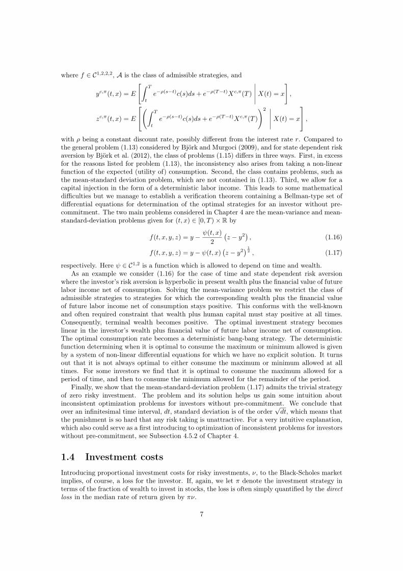
respectively. Here ψ ∈ C1,2 is a function which is allowed to depend on time and wealth.As an example we consider (1.16) for the case of time and state dependent risk aversion

where the investor’s risk aversion is hyperbolic in present wealth plus the financial value of futurelabor income net of consumption. Solving the mean-variance problem we restrict the class ofadmissible strategies to strategies for which the corresponding wealth plus the financial valueof future labor income net of consumption stays positive. This conforms with the well-knownand often required constraint that wealth plus human capital must stay positive at all times.Consequently, terminal wealth becomes positive. The optimal investment strategy becomeslinear in the investor’s wealth plus financial value of future labor income net of consumption.The optimal consumption rate becomes a deterministic bang-bang strategy. The deterministicfunction determining when it is optimal to consume the maximum or minimum allowed is givenby a system of non-linear differential equations for which we have no explicit solution. It turnsout that it is not always optimal to either consume the maximum or minimum allowed at alltimes. For some investors we find that it is optimal to consume the maximum allowed for aperiod of time, and then to consume the minimum allowed for the remainder of the period.

Finally, we show that the mean-standard-deviation problem (1.17) admits the trivial strategyof zero risky investment. The problem and its solution helps us gain some intuition aboutinconsistent optimization problems for investors without pre-commitment. We conclude thatover an infinitesimal time interval, dt, standard deviation is of the order

√dt, which means that

the punishment is so hard that any risk taking is unattractive. For a very intuitive explanation,which also could serve as a first introducing to optimization of inconsistent problems for investorswithout pre-commitment, see Subsection 4.5.2 of Chapter 4.

1.4 Investment costsIntroducing proportional investment costs for risky investments, ν, to the Black-Scholes marketimplies, of course, a loss for the investor. If, again, we let π denote the investment strategy interms of the fraction of wealth to invest in stocks, the loss is often simply quantified by the directloss in the median rate of return given by πν.

7

However, there seems to be a lack of more serious approaches to quantify the impact ofinvestment costs. Therefore, we return in Chapter 5 to the original problem of Merton, andconsider (1.1) for an investor with CRRA preferences for terminal wealth (no consumption).This opens up the possibility to do a risk-adjusted evaluation of investment costs. By use of aValue at Risk measure Guillén et al. (2013) also perform a risk-adjusted evaluation of investmentcosts.

The main assumption essential for the analysis in Chapter 5 is that no investor can beatthe market. Something many expensive mutual fund managers claim when asked by customersabout the high fees they demand. In other words, we assume a zero correlation between costratios and expected investment returns. Something showed to be true by a vast amount ofliterature (see Chapter 5, Subsection 5.1, for references).

The point of view taken in Chapter 5 is the situation of declining investment costs. Oneshould bear in mind the situation of an investor who has handed over his savings to a mutualfund that on his behalf invests the money. For the service the mutual fund charges a fee.Under the assumption of the existence of another fund charging a lower fee and performing (inexpectation) equally well, we quantify the impact of paying the higher fee. We call an investortaking risk aversion into account, by use of a concave strictly increasing utility function, whendeciding upon an investment strategy a sophisticated investor. The first main point of Chapter 5is:

• The sophisticated investor experiences a greater change in the rate of return induced by achange in investment costs compared to the direct loss.

• This is so since the risk aversion of the investor optimally dictates a part of the money theinvestor saves by paying less investment costs to be invested in stocks.

The evaluation is based on an indifference compensation ratio defined as the minimum relativeincrease in the initial wealth the investor demands in compensation to accept incurring the higherinvestment costs. Let ν1 and ν2 denote the higher and lower cost ratio, respectively. Formally,we define the indifference compensation ratio ICR(ν1,ν2) by the relation

supπE[u(X(ν2,π)(T )

) ∣∣∣X(ν2,π)(0) = x0

]= sup

πE[u(X(ν1,π)(T )

) ∣∣∣X(ν1,π)(0) = x0(1 + ICR(ν1,ν2)

)]. (1.18)

We show that for a CRRA function (µ) the measure is equivalent to the relative change incertainty equivalents. We compare this measure to the present value of the investment costs theinvestor is expected to pay over the investment horizon, evaluated as a fraction of the initialwealth. We interpret the latter value as the direct effect of investment costs, and the differencebetween the direct effect and the ICR-value, as the indirect effect of investment costs. Forrealistic market parameters the conclusion is rather surprising. For an investor, who on onehand has the possibility to invest through a mutual fund being charged 0.6% in investmentcosts, but who invest through a mutual fund charging him investment costs at a ratio equal to1.4%, with an optimally stock allocation of 60%, the indirect effect is between 50–100% of thedirect effect, dependent on the investment horizon (longer horizon, higher indirect effect).

Finally, the approach allows us to answer a related question: Is the investment strategy orthe size of the investment costs of most importance? Concretely, we study an investor facinghigh investment costs and an optimal investment strategy (w.r.t. his risk profile), and ask whichinvestment strategies the investor is willing to accept if he at the same time is offered lowerinvestment costs. The conclusion, the second main point of Chapter 5, is very clear

• Independent of the time horizon, the particular allocation towards risky stocks seems tobe of very little importance compared to the size of investment costs.

8

To demonstrate the magnitude consider again the investor who invests through the expensivemutual fund charging him high investment costs at rate 1.4%, with an optimally stock alloca-tion of 60%. For realistic market parameters we calculate that for the investor who shifts tothe cheaper fund offering to manage his savings charging him a lower cost rate off 0.6%, anyinvestment strategy allocating between 28% and 129% of his wealth in stocks makes him equallyor better of. This examples quantifies why collective investment scheme with a common strategyfor all members, thereby maintaining costs low, could be preferable for many investors.

1.5 A collective with-profit pension schemeIn the last chapter of this thesis, Chapter 6, we derive several results for discrete-time randomwalks with continuous innovations. Of special interest is the entrance time (time of return to ori-gin) distribution. We derive an expansion formula for the entrance time probabilities, a formulafor the nth derivative of the generating function, a formula for the nth moment of the waitingtimes, and formulas for the conditional undershoot process given the first entrance time. Allquantities are also considered for the stationary process.

First, the analysis of the discrete-time random walk with continuous innovations is triggeredby the desire to analyze the investment decision for a so called with-profit collective pensionscheme, a very widespread pension product in e.g. the Nordic countries and the Netherlands.

In Chapter 6 each contribution is split into a part giving a guaranteed payment and a partinvested in a, possibly leveraged, investment portfolio. Define the funding ratio F by

F (t) =A(t)

R(t),

where A(t) denotes the total assets of the fund and R(t) the financial value of the guaranteedbenefits, known as the reserve. In our model both contributions and benefits are paid andwithdrawn, respectively, such that the funding ratio is not affected, i.e. the product is fair.The difference between the total assets and the reserve, A(t) − R(t), is known as the bonuspotential. It is the bonus potential which is invested in stocks (possible leveraged). The productis with-profit in the sense that all guaranteed payments are increased, known as bonus, whenthe funding ratio exceeds a given threshold κ. The decision to attribute bonus or not is takenat a set of equidistant discrete set of time points 0 = t0 < t1 < . . .. We assume for simplicitythat contributions and benefits also fall at these times. After (possible) bonus attribution thefunding ratio becomes minF (ti), κ.

A simple version of the pension product, to be considered as an example in Chapter 6, is thecase of a unit contribution made at time t = 0 for a benefit paid out in its entirety at time t = T(retirement). In this case the benefit at retirement becomes

F (T )

F (0)erT

T∏i=1

(1 + rBi

), (1.19)

where rBi is the possible bonus attribution at time ti.It follows from Preisel et al. (2010) that in a Black-Scholes market model the funding ratio

process becomes a (discrete-time) Markov chain with dynamics

Fi = min(Fi−1 − 1)e(Cµ− 1

2C2σ2

Z)∆+CσZ

√∆Ui + 1, κ

, (1.20)

where the Ui’s are i.i.d. standard normal variables, µ and σZ the expected excess return andvolatility on stocks, respectively, and C the fraction of the bonus potential invested in stocks.The funding ratio process (1.20) has also been studied by Preisel et al. (2010) and Kryger (2010)

9

using a number of analytical approximations. In contrast, Chapter 6 relies almost exclusivelyon exact results. We consider the following transformation

Yn = − log

(Fn − 1

κ− 1

)for n ∈ N0. (1.21)

This turns the funding ratio process (1.20) into the one-sided random walk

Yn = (Yn−1 +Xn)+, (1.22)

where the Xn’s are i.i.d. normally distributed with mean −(Cµ− 1

2C2σ2

Z

)∆ and variance

C2σ2Z∆. Note that Fn = κ corresponds to Yn = 0, while funding ratios close to one corre-

spond to high values of Y . In other words, bonus is attributed whenever the Y -process returnsto zero. Along with Y we also consider the (unrestricted) random walk

S0 = 0 and Sn = Sn−1 +Xn for n ∈ N, (1.23)

with the same Xn’s as in (1.22).

Now with the model of inspiration in place we return to a general discrete-time random walkwith continuous innovations. First we consider the entrance time probabilities

τn = P (τ− = n) = P (S1 > 0, . . . , Sn−1 > 0, Sn ≤ 0). (1.24)

A central concept in Chapter 6 is the set of integer partitions of a given order n ≥ 1 given by

Dn =

(σ1, . . . , σn)

∣∣∣σ1 ∈ N0, . . . , σn ∈ N0,

n∑i=1

iσi = n

,

where N0 = 0, 1, 2, . . ..First, we show by use of the generating function, τ(s) =

∑∞n=1 τns

n, and the Theorem ofSparre-Andersen (see Theorem 6.2.1) which expresses the generating function in terms of themarginal probabilities P (Sn ≤ 0), that the first entrance time probabilities (1.24) can be com-puted as a partition sum over the marginal probabilities of the random walk, see Theorem 6.2.3.The Theorem is also implicit in the paper by Spitzer (1956), but in Chapter 6 we give a simplerself-contained proof.

Second, we derive an expression for the n’th derivative of the generating function for theentrance times, τ (n)(s), see Theorem 6.2.5, which we subsequently use to derive a formula forthe factorial moments, E((τ−)n), see Theorem 6.2.6. Again the results consist of a partition sumover marginal probabilities of the random walk. Both results are new and presented for the firsttime in Chapter 6.

Third, we derive formulas for the characteristic function of the position of the random walkconditioned on entrance at time n, E

(eiζSn |τ− = n

), see Theorem 6.2.8, and on entrance after

time n, E(eiζSn |τ− > n), see Theorem 6.2.9. The results consist of partition sum formulas ofpartial expectations for the characteristic function of the random walk. The first of these resultsis known, but the proof offered by Chapter 6, which builds upon Theorem VII 4.1 of Asmussen(2003) which is a generalization of the Sparre-Andersen theorem to combined generating andcharacteristic functions (see Theorem 6.2.7), is new. The second result is new and presented forthe first time in Chapter 6.

Returning to the pension model our prime interest is the stationary process. The stationaryprocess has the interpretation of an average scenario. We therefore define by

T1 = infn ≥ 1 : Fn = κ = infn ≥ 1 : Yn = 0, (1.25)

10

and, recursively, for k ≥ 2

Tk = infn ≥ 1 : FTk−1+n = κ = infn ≥ 1 : YTk−1+n = 0, (1.26)

the time between consecutive bonus attributions. The results of Theorem 6.2.3–6.2.9 is connectedto the case where F0 = κ. In Subsection 6.4 the case F0 ∼ π, i.e. the stationary process, isunder consideration. Using the results for the F0 = κ case more or less explicit closed formsolutions, for the first entrance time probabilities and the characteristic function of the positionof the random walk conditioned on entrance at time n, are derived for the stationary process.The key to analyzing the pension model is (1.21). For F0 = κ the events (T1 = n) and (τ− = n)are identical and on this event the bonus percentage becomes

rBn =κ− 1

κ

(e−Sn − 1

).

Likewise on F0 = κ the events (T1 > n) and (τ− > n) are identical and on this event

Fn = (κ− 1)e−Sn + 1.

By these quantities we analyze the first bonus time probabilities (the time between consecutivebonus attributions), the probability distribution of the number of bonuses, the expected bonussize, and the expected funding ratio. Furthermore, these results allow us to analyze the mean andvariance of the pension benefit (1.19). For an average scenario (in stationarity) we develop anexact simulation approach and show that the expected pension benefit admits an interior solutionin the investment strategy C. At some point, taking more risk results in a lower expected payoff.This is in great contrast to the prevailing idea that taking more risk should be compensatedby higher expected returns, but the interpretation is clear. High allocation towards risky assetsimplies a high conditional expected bonus, but comes with the risk of being trapped at lowfunding ratios for a long time (rare bonuses). The analysis of Chapter 6 presents the optimaltrade-off between the two effects.

11

12

2. Optimal consumption and investmentwith labor income andEuropean/American capital guarantee

Abstract: We present the optimal consumption and investment strategy for aninvestor, endowed with labor income, searching to maximize utility from consumptionand terminal wealth when he is restricted to fulfill a binding capital constraint of aEuropean (constraint on terminal wealth) or an American (constraint on the wealthprocess) type. In both cases the optimal strategy is proven to be of the option basedportfolio insurance type. The optimal strategy combines a long position in the optimalunrestricted allocation with a put option. In the American case, where the investor isrestricted to fulfill a capital guarantee at every intermediate time point over the intervalof optimization, we prove that the investor optimally changes his budget constraint forthe unrestricted allocation whenever the constraint is active. The strategy is explainedin a step by step manner and graphically illustrations are presented in order to supportthe intuition and to compare the restricted optimal strategy with the unrestrictedoptimal counterpart.

Keywords: Stochastic control; martingale method; option based portfolio insur-ance; American put option; human capital; borrowing constraint; CRRA utility.

2.1 IntroductionWe study the optimal consumption and investment decision problem for an investor, endowedwith deterministic labor income, who faces an American capital guarantee restriction. An Amer-ican capital guarantee is a capital constraint which is valid at all time points in the time intervalof consideration. Likewise, we refer to at capital guarantee only valid at the terminal time pointas a European capital guarantee. The names are inherited from the option framework, i.e. fromAmerican and European options. The problem is set in a continuous-time frictionless Black-Scholes market and the investor measures his tolerance towards risk by a constant relative riskaversion utility function.

The corresponding free consumption and investment decision problem, where the investoris not restricted to fulfill any capital guarantee, is a very well understood problem, see Merton(1969) and Merton (1971). Traditionally, such problems have been solved using stochastic dy-namic programming. However, stochastic dynamic programming becomes difficult when addinga capital constraint since the value function, in addition to a stochastic differential equation,must satisfy some boundary condition whenever the wealth is at the boundary. This leaves uswith a non-linear Hamilton-Jacobi-Bellman equation for which the existence of a solution has tobe established.

Consequently, this article uses instead the martingale methodology developed by Cvitanicet al. (1987), Cox and Huang (1989) and Cox and Huang (1991). We adopt the ideas from El-Karoui et al. (2005) and use the put option based approach to derive the optimal consumptionand investment strategy for an investor who faces an American capital guarantee restrictiondefined as a deterministic function. It turns out that the optimal strategy consists of investinga part of the initial total wealth1 in the corresponding optimal unrestricted allocation and the

1Initial wealth plus the financial value of future labor income.

13

remainder in a put option written on the optimal unrestricted portfolio. In order for this strategyto be admissible we show that the investor must adjust the portfolio continuously whenever theconstraint is active. This result is similar to the one of El-Karoui et al. (2005), although theydo not allow for consumption and labor income. The main contribution of this article is that weshow that the put option based approach can also be carried out to find the optimal strategyin the case including consumption and labor income. Clearly the introduction of consumptionleads to further mathematical difficulties, but in fact nor is the introduction of deterministic la-bor income trivial. One important thing to note is that, in contrast to the unrestricted problemof Merton, being endowed with labor income or being endowed with an initial wealth enlargedby the financial value of future labor income is not equivalent when considering an Americancapital guarantee restriction. In the case of an American capital guarantee the latter case ispreferable. This indicates that adding deterministic labor income to the setting considered inEl-Karoui et al. (2005) is not as easy as it may seem. The strategy actually differs from the caseexcluding deterministic labor income. We show that adding deterministic labor income can behandled by buying an insurance, a put option, with a strike price substantially different fromthe one obtained by El-Karoui et al. (2005). To ease the understanding of the optimal strategyderived the analysis also contains a step by step explanation of the optimal strategy togetherwith a numerically graph-based explanation. In the special case of a restriction to borrow againstfuture labor income (an American capital guarantee equal to zero), we compare numerically therestricted solution with the unrestricted counterpart.

A reasonable question is whether a wealth constraint is relevant for an individual endowedwith deterministic labor income. As mentioned, for the unrestricted problem the investor opti-mally sells his future labor income in the market and acts as if he had an enlarged initial wealth.Consequently, the investor’s terminal wealth becomes positive, but the investor’s wealth maybecome negative at some point in time before terminal time. If labor income really is determin-istic one could argue that this is perfectly acceptable. The motivation of generally introducingan American capital guarantee, and specifically to analyze the case of a restriction to borrowagainst future labor income, is however manifold. Consider for example the lending business.In reality you can borrow a great amount of money from the bank to buy a house if you arethe receiver of a (possible stochastic) labor income. The reason is that you invest your loanin the house and thereby maintain a positive wealth. Of course the value of the house coulddrop, but since the loan comes with an amortization plan2 the wealth stays positive (with a highprobability). You can also get a mortgage loan from the bank to finance consumption. On theother hand it is almost impossible to get a loan from the bank to finance pure consumption if youcan not provide security for the loan3. Why is that? Of course this is partly because the bankconsider your labor income stochastic (e.g. you might lose your job), but there are many otherreasons. Most of them are connected to obvious reasons as moral hazards, adverse selection andadministration problems. Or one could say that the bank just does not want to take on thatrisk. This paper is motivated by the real life situation many individuals face. As an individualyou do not consider your labor income as stochastic. At least you do not act as if you do. This ispartly because it is very hard to model labor income since the list of relevant stochastic variablesto include in the modulation should be very long. The modeling should, among other things,include future political decisions, possible world wars, personal accidents (you may become dis-able), your mortality (you may die) and the demand of tomatoes (if you make a living of sellingtomatoes). In addition many people actually have a very stabile and secure labor income, andthereby have a very strong belief about how their life long labor income would be. If this wasnot true, why are more people not buying unemployment insurance? Summing up, the questionmany individuals face is: You consider your labor income deterministic and you act responsiblyas a good citizen. Unfortunately the bank does not agree with you and consequently the bank

2In addition most banks require the investor himself to provide (say) 5 percent funding.3In some countries this is actually possible, but since expenses are incredible high we assume that the investor

does not consider this as an opportunity.

14

is only willing to issue a loan if you invest in such a way that they do not stand the chance ofending up with a loss (your total assets has to be positive at all times). Given this situationhow should you optimally consume and invest? This is one interpretation of the question ofconsideration in this article.

Furthermore, the problem studied in this article is, putting consumption equal to zero, highlyrelevant for many financial institutions. The most obvious example is pension companies whichare forced by law (by the Financial Supervisory Authority (FSA)) to fulfill certain capital re-quirements at all times. In such a framework labor income has the interpretation as pensioncontributions and the American capital guarantee, introduced by the FSA, puts restrictions onthe pension company’s actions.

The paper by Lakner and Nygren (2006) consider a similar problem. They maximize ex-pected utility from consumption and terminal wealth when both the consumption rate andterminal wealth must not fall below a given minimum consumption level and a minimum wealthlevel, respectively. This is handled by dividing initial wealth into two parts, x1 and x2, and thensolving the constrained pure consumption problem with initial wealth x1 and the constrainedpure portfolio problem with initial wealth x2. The superposition of the actions for the twoconstrained subproblems is then shown to be the optimal strategy provided that x1 and x2 arechosen such that the "marginal expected utilities" from the two constrained subproblems areidentical. In this article we do not consider a minimum level of consumption constraint since wedo not want the consequence of the introduction of an American capital guarantee to be blurredby other constraints. One could, using the results obtained in this article, apply the approachof Lakner and Nygren (2006) to solve such a problem.

Using different approaches, the restriction to borrow against future labor income has beenanalyzed in different settings with spanned stochastic income rate. He and Pagès (1993) useduality theory to show the existence of an optimal strategy and find that the presence of a liq-uidity constraint has a smoothing effect on the optimal consumption. El-Karoui and Jeanblanc(1998) introduce the concept of super strategies to show that the fair-value, defined as the min-imal investment required to replicate a consumption investment strategy with a super strategy,consists of investing a part of the initial wealth in a free portfolio and to use the remaining partto buy an American put option on this underlying asset. A setting with un-spanned stochasticincome is analyzed by Duffie and Zariphopoulou (1993), Duffie et al. (1997), Koo (1998) andMunk (2000) who also gives a very complete overview of the field as a whole.

The paper is organized as follows: In Section 2.2 we present the economic model, the conceptof admissible strategies and other preliminaries. In Section 2.3 we solve the unrestricted problemusing the martingale technique. As an inspirational example we solve, in Section 2.4, the optimalconsumption and investment decision problem when the investor is restricted to fulfill a bindingterminal capital guarantee (any terminal guarantee strictly greater than zero), also known as aEuropean capital guarantee. Using the building blocks derived in Section 2.3 and 2.4, and thetheory of American put options in a Black-Scholes market, we construct in the main section,Section 2.5, an admissible put option based portfolio insurance strategy. We show that thisstrategy is optimal for the consumption and investment decision problem where the investoris restricted to fulfill an American capital guarantee. Finally, in Subsection 2.5.3 graphicalillustrations of the optimal restricted strategy together with a comparison with the optimalunrestricted strategy are presented for the special case of a restriction to borrow against futurelabor income.

15

2.2 SetupConsider a frictionless Black-Scholes market consisting of a bank account, B, with risk-free shortrate, r, and a risky stock, S, with dynamics given by

dB(t) = rB(t)dt, B(0) = 1,

dS(t) = αS(t)dt+ σS(t)dW (t), S(0) = s0 > 0.

Here α, σ, r > 0 are constants and it is assumed that α > r. The process W is a standardBrownian motion on an abstract probability space (Ω,F , P ) equipped with the filtration FW =(FW (t)

)t∈[0,T ]

given by the P -augmentation of the filtration σW (s); 0 ≤ s ≤ t, ∀t ∈ [0, T ].

We consider an investor endowed with a continuous deterministic labor income of rate ℓ, aninitial amount of money x0 and a time horizon of interest [0, T ], T > 0 . Over the time interval,[0, T ], the investor has the opportunity to continuously consume a fraction of his wealth and toinvest his wealth in the Black-Scholes market. More specific, let c denote the rate of consumptionand let π denote the fraction of wealth to be invested in the risky asset, S. For a given strategy,(c, π), the wealth process of the investor, (X(t))t∈[0,T ], is given by the dynamics

dX(t) = [(r + π(t)(α− r))X(t) + ℓ(t)− c(t)]dt+ σπ(t)X(t)dW (t), t ∈ [0, T ), (2.1)X(0) = x0 ≥ 0.

We assume the consumption rate c(t), t ∈ [0, T ], to be a non-negative, FW (t)-adapted processwith

∫ T

0c(t)dt < ∞ a.s., and the investment strategy π(t), t ∈ [0, T ], to be an FW (t)-adapted

process such that (2.1) has a unique solution X(t), t ∈ [0, T ], satisfying∫ T

0(π(t)X(t))2dt <

∞ a.s.. We have, ∀t ∈ [0, T ], the representation

X(t) = x0ert +

∫ t

0

er(t−s)[π(s)X(s)(α− r) + ℓ(s)− c(s)]ds+

∫ t

0

er(t−s)σπ(s)X(s)dW (s).

It is well known that in the Black-Scholes market the equivalent martingale measure, Q, is uniqueand given by the Radon-Nikodym derivative

dQ(t)

dP (t)= Λ(t) := exp

(−(α− r

σ

)W (t)− 1

2

(α− r

σ

)2

t

), t ∈ [0, T ],

and that the process WQ given by WQ(t) = W (t) + α−rσ t, t ∈ [0, T ], is a standard Brownian

motion under Q. We get that the investor’s wealth can be represented, ∀t ∈ [0, T ], by

X(t) = x0ert +

∫ t

0

er(t−s)(ℓ(s)− c(s))ds+

∫ t

0

er(t−s)σπ(s)X(s)dWQ(s). (2.2)

Definition 2.2.1. Define the set of admissible strategies, denoted by A, as the consumption andinvestment strategies for which the corresponding wealth process given by (2.2) is well-defined,

X(t) + g(t) ≥ 0, ∀t ∈ [0, T ], (2.3)

where g is the time t financial value of future labor income defined by g(t) :=∫ T

te−r(s−t)ℓ(s)ds,

and

EQ

[∫ T

0

e−rsσπ(s)X(s)dWQ(s)

]= 0. (2.4)

16

The technical condition (2.4) is equivalent to the condition that under Q the process∫ t

0

e−rsσπ(s)X(s)dWQ(s), t ∈ [0, T ],

is a martingale (in general it it only a local martingale, and also a supermartingale if (2.3) isfulfilled, see e.g. Karatzas and Shreve (1998)). From this we conclude that (2.4) insures that(c, π) ∈ A if and only if X(T ) ≥ 0 and, ∀t ∈ [0, T ],

X(t) + g(t) = EQ

[∫ T

t

e−r(s−t)c(s)ds+ e−r(T−t)X(T )

∣∣∣∣∣ FW (t)

].

At time zero this means the strategies have to fulfill the budget constraint

x0 + g(0) = EQ

[∫ T

0

e−rtc(t)dt+ e−rTX(T )

]. (2.5)

For latter use we state the following remark.

Remark 2.2.1. Define

Z(t) :=

∫ t

0

e−rs(c(s)− ℓ(s))ds+ e−rtX(t), t ∈ [0, T ]. (2.6)

By (2.2) we have that condition (2.4) is fulfilled if and only if Z is a martingale under Q. Thenatural interpretation is that under Q the discounted wealth plus discounted consumption excessof labor income should be a martingale. It is useful to note that if Z is a martingale under Qthe dynamics of X can be represented in the form

dX(t) = [(rX(t) + ℓ(t)− c(t)]dt+ ϕ(t)dWQ(t), t ∈ (0, T ], (2.7)

for some FW (t)-adapted process ϕ. Moreover, if the dynamics of X can be represented in theform given by (2.7) for some FW (t)-adapted process ϕ satisfying ϕ(t) ∈ £2, ∀t ∈ [0, T ], then Zis a martingale under Q.

Finally, by condition (2.3) we allow the wealth process to become negative, as long as it doesnot exceed (in absolute value) the financial value of future labor income. Note that condition(2.3) puts a lower boundary on the wealth process and therefore rules out doubling strategies(see e.g. Karatzas and Shreve (1998)).

2.3 The unrestricted control problemFor the rest of this paper we assume that the investor’s preferences can be stated in terms of aconstant relative risk aversion (CRRA) utility function u : [0,∞) → [−∞,∞) in the form

u(x) =

xγ

γ , if x > 0

limx0xγ

γ , if x = 0,

for some γ ∈ (−∞, 1)\0. In the unrestricted control problem, known as Merton’s problem(Merton (1969) and Merton (1971)), the investor seeks to find the strategy fulfilling the supre-mum

sup(c,π)∈A′

E

[∫ T

0

e−∫ t0β(s)dsu(c(t))dt+ e−

∫ T0

β(s)dsu(X(T ))

], (2.8)

17

where X(0) = x0 and β is a deterministic function representing the investor’s time preferences.The supremum in (2.8) is taken over the subset of the admissible strategies, referred to as thefeasible strategies, defined by

A′ :=

(c, π) ∈ A

∣∣∣∣∣ E[∫ T

0

e−∫ t0β(s)ds min(0, u(c(t)))dt+ e−

∫ T0

β(s)ds min(0, u(X(T )))

]> −∞

,

(2.9)

i.e. it is allowed to draw an infinite utility from a strategy (c, π) ∈ A′, but only if the expectationover the negative parts of the utility function is finite. Clearly, for γ ∈ (0, 1) we have that A andA′ coincide.

The unrestricted control problem (2.8) can be solved using either the conventional Hamilton-Jacobi-Bellman (HJB) method (see e.g. Fleming and Richel (1975)) or the newer martingalemethod (see Cvitanic et al. (1987), Cox and Huang (1989) and Cox and Huang (1991)). Despitethe fact that this is most easily done using the HJB-method we now sketch the solution to (2.8)in terms of the martingale method. We do so because the solution to the corresponding Ameri-can capital guarantee version of (2.8), presented in Section 2.5, is based on terms derived fromthe martingale method.

Define the inverse of the derivative of u as the function I : (0,∞] → [0,∞) and define theadjusted state price deflator

H(t) := Λ(t)e∫ t0(β(s)−r)ds.

Since I is continuous and decreasing and maps (0,∞] onto [0,∞) we get the useful result thatthere exist a unique constant ξ∗ > 0 such that (see. e.g. Karatzas and Shreve (1998))

EQ

[∫ T

0

e−rtI(ξ∗H(t))dt+ e−rT I(ξ∗H(T ))

]= x0 + g(0). (2.10)

Finally, note that from the concavity of u and u′(I(z)) = z we get

u(x) ≤ u(I(z))− z(I(z)− x), ∀x ≥ 0, z > 0. (2.11)

Now, take an arbitrary strategy (c, π) ∈ A′ with corresponding wealth process (X(t))t∈[0,T ] asgiven. Using (2.11), the budget constaint (2.5) and finally (2.10) we get that

E

[∫ T

0

e−∫ t0β(s)dsu(c(t))dt+ e−

∫ T0

β(s)dsu(X(T ))

]

≤ E

[∫ T

0

e−∫ t0β(s)dsu(I(ξ∗H(t)))dt+ e−

∫ T0

β(s)dsu(I(ξ∗H(T )))

].

Since (c, π) was arbitrarily chosen we conclude that the candidate optimal strategy (c∗, π∗) isgiven by

c∗(t) = I(ξ∗H(t)), (2.12)X∗(T ) = I(ξ∗H(T )), (2.13)

where X∗(T ) is the corresponding terminal wealth obtained from using the strategy (c∗, π∗). Byuse of the martingale representation theorem (see e.g. Karatzas and Shreve (1991)) we obtain(after some rather cumbersome calculations)

c∗(t) =X(t) + g(t)

f(t), (2.14)

π∗(t)X∗(t) =1

γ

α− r

σ2(X∗(t) + g(t)), (2.15)

18

where

f(t) =

∫ T

t

e−∫ st[r(y)+β(y)]dyds+ e−

∫ Tt

[r(y)+β(y)]dy,

with r(y) = γγβ(y) −

γγ r −

12

γ(1−γ)2

(α−rσ

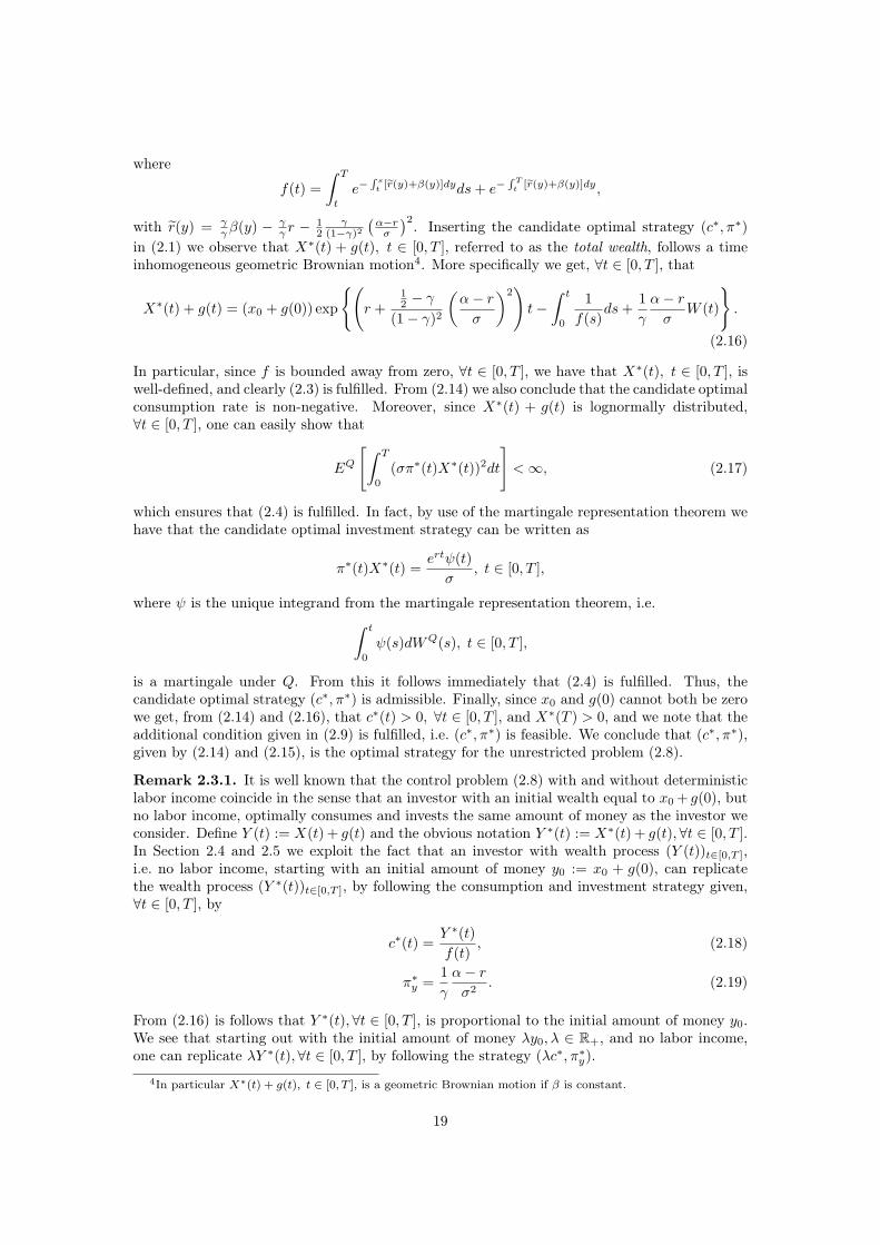
)2. Inserting the candidate optimal strategy (c∗, π∗)

in (2.1) we observe that X∗(t) + g(t), t ∈ [0, T ], referred to as the total wealth, follows a timeinhomogeneous geometric Brownian motion4. More specifically we get, ∀t ∈ [0, T ], that

X∗(t) + g(t) = (x0 + g(0)) exp

(r +

12 − γ

(1− γ)2

(α− r

σ

)2)t−

∫ t

0

1

f(s)ds+

1

γ

α− r

σW (t)

.

(2.16)

In particular, since f is bounded away from zero, ∀t ∈ [0, T ], we have that X∗(t), t ∈ [0, T ], iswell-defined, and clearly (2.3) is fulfilled. From (2.14) we also conclude that the candidate optimalconsumption rate is non-negative. Moreover, since X∗(t) + g(t) is lognormally distributed,∀t ∈ [0, T ], one can easily show that

EQ

[∫ T

0

(σπ∗(t)X∗(t))2dt

]<∞, (2.17)

which ensures that (2.4) is fulfilled. In fact, by use of the martingale representation theorem wehave that the candidate optimal investment strategy can be written as

π∗(t)X∗(t) =ertψ(t)

σ, t ∈ [0, T ],

where ψ is the unique integrand from the martingale representation theorem, i.e.∫ t

0

ψ(s)dWQ(s), t ∈ [0, T ],

is a martingale under Q. From this it follows immediately that (2.4) is fulfilled. Thus, thecandidate optimal strategy (c∗, π∗) is admissible. Finally, since x0 and g(0) cannot both be zerowe get, from (2.14) and (2.16), that c∗(t) > 0, ∀t ∈ [0, T ], and X∗(T ) > 0, and we note that theadditional condition given in (2.9) is fulfilled, i.e. (c∗, π∗) is feasible. We conclude that (c∗, π∗),given by (2.14) and (2.15), is the optimal strategy for the unrestricted problem (2.8).

Remark 2.3.1. It is well known that the control problem (2.8) with and without deterministiclabor income coincide in the sense that an investor with an initial wealth equal to x0+ g(0), butno labor income, optimally consumes and invests the same amount of money as the investor weconsider. Define Y (t) := X(t) + g(t) and the obvious notation Y ∗(t) := X∗(t) + g(t),∀t ∈ [0, T ].In Section 2.4 and 2.5 we exploit the fact that an investor with wealth process (Y (t))t∈[0,T ],i.e. no labor income, starting with an initial amount of money y0 := x0 + g(0), can replicatethe wealth process (Y ∗(t))t∈[0,T ], by following the consumption and investment strategy given,∀t ∈ [0, T ], by

c∗(t) =Y ∗(t)

f(t), (2.18)

π∗y =

1

γ

α− r

σ2. (2.19)

From (2.16) is follows that Y ∗(t),∀t ∈ [0, T ], is proportional to the initial amount of money y0.We see that starting out with the initial amount of money λy0, λ ∈ R+, and no labor income,one can replicate λY ∗(t),∀t ∈ [0, T ], by following the strategy (λc∗, π∗

y).

4In particular X∗(t) + g(t), t ∈ [0, T ], is a geometric Brownian motion if β is constant.

19

Note that the optimal strategy (c∗, π∗) guarantees that X∗(t) > −g(t),∀t ∈ [0, T ]. This isin some sense a direct consequence of CRRA utility. Loosely speaking, the marginal increasein utility is going to infinity as terminal wealth is going to zero, i.e. a terminal wealth equal tozero cannot be optimal. To be able to avoid this in all scenarios the investor simply ensuresthat X∗(t) > −g(t),∀t ∈ [0, T ]. As mentioned in Section 2.1, one should also notice thatthe formulation of problem (2.8) assumes that the bank allows the investor to have a negativewealth at any given time point t ∈ (0, T ). This will in reality, due to reasons discussed inthe introduction, likely not be the case. Furthermore, most investors tend to have some sortof preference or demand for a capital guarantee. The most obvious example is that pensioncompanies often are required by authorities (FSA) to fulfill a certain American capital guarantee.Jensen and Sørensen (2001) quantify that an individual facing a (European) mandatory minimuminterest rate guarantee, as an integrated part of the pension contract, is forced to invest in anembedded put option. They argue that the investor may face a constraint on the feasible set ofportfolio choices which may induce a significant utility loss.

Including an American capital guarantee to problem (2.8) is the main problem of interest inthis article. Inspired by El-Karoui et al. (2005) we, as an inspirational example, start out bysolving the easier case including a binding European capital guarantee. This problem was firstsolved by Teplá (2001).

2.4 The European capital guarantee control problemConsider the problem

sup(c,π)∈A′

E

[∫ T

0

e−∫ t0β(s)dsu(c(t))dt+ e−

∫ T0

β(s)dsu(X(T ))

], (2.20)

under the capital constraint X(T ) ≥ K. In Section 2.3 we saw that K ≤ 0 is a non-bindingconstraint. Note that in order for the European capital guarantee problem to be solvable andnon-trivial5 we must demand that

K < erT (x0 + g(0)). (2.21)

Proposition 2.4.1 presents the optimal strategy for problem (2.20). The strategy is based ona so-called option based portfolio insurance (OBPI) written on a ’budget-adjusted’ version of theoptimal portfolio derived for the unrestricted problem. First, we need some notation: Denoteby P e

X(t, T,K) the time t value of a European put option with strike price K and maturity Twritten on a portfolio (X(s))s∈[t,T ]. As in Section 2.3 X∗(t), c∗(t) and π∗(t), t ∈ [0, T ], denotethe optimal wealth, the optimal consumption strategy and the optimal investment strategy forthe unrestricted problem (2.8), respectively.

Proposition 2.4.1. Consider the strategy (c, λY ∗) where, ∀t ∈ [0, T ],

c(t) :=λY ∗(t)

f(t)= λc∗(t),

Y ∗(t) := X∗(t) + g(t),

combined with a position in a European put option with strike price K and maturity T writtenon the portfolio (λY ∗(s))s∈[t,T ], where λ is determined by the budget constraint

X(λ)(0) := λ(x0 + g(0)) + P eλY ∗(0, T,K)− g(0) = x0. (2.22)

5In the case of equality in (2.21) the investor has no choice but to invest all his wealth including labor incomein the risk-free short rate to be sure to fulfil the capital guarantee.

20

Observing that Y ∗(T ) = X∗(T ), it follows that the terminal value of the corresponding optionbased portfolio insurance becomes

X(λ)(T ) := λX∗(T ) + (K − λX∗(T ))+= max (λX∗(T ),K) , (2.23)

i.e. the European capital guarantee is fulfilled. We have that

1. The strategy is affordable, i.e. there exist a unique λ ∈ (0, 1) such that the budget constraint(2.22) is fulfilled.

2. The strategy is optimal for the European capital guarantee control problem given by (2.20).

Note that, clearly, the strategy in Proposition 2.4.1 is feasible since the unrestricted strategy(c∗, π∗) given in Section 2.3 is feasible.

Remark 2.4.1. To clarify, following the strategy(c, X(λ)

)given by Proposition 2.4.1 means

that the investor should:

1. Take a loan of size g(0) and reserve the labor income to pay back the loan over the timeinterval [0, T ].

2. Reserve the initial amount of money λ(x0+g(0)) to follow the consumption and investmentstrategy (c, π) given by

c(t) := λc∗(t),

π := π∗y .

Doing this the investor replicates the portfolio λY ∗(t),∀t ∈ [0, T ], i.e. the investor replicatesthe terminal value λY ∗(T ) = λX∗(T ) (see Remark 2.3.1).

3. Use the remaining initial amount of money (1−λ)(x0+g(0)) to buy a European put optionwith strike price K and time to maturity T written on the portfolio (λY ∗(t))t∈[0,T ].

The European put option is likely not to be sold in the market, but since the market is completeand frictionless such options can be replicated dynamically by a Delta-hedge, i.e. the optimalinvestment strategy π(t), t ∈ [0, T ], is given by

π(t)X(λ)(t) =

(1 +

∂

∂yP eλY ∗(t, T,K)

)π∗yλY

∗(t).

Since the European put option has an opposite exposure to changes in the underlying portfolioλY ∗(t), t ∈ [0, T ], we note that the total amount of money to invest in the risky asset, S,becomes smaller when we introduce a European capital guarantee to the control problem (2.8).

Proof of affordability. First note that X(λ)(T ) = max (λX∗(T ),K) is non-decreasing in λ withvalues in [K,∞). For λ1 < λ2 we get

0 ≤ X(λ2)(T )− X(λ1)(T ) ≤ (λ2 − λ1)X∗(T ).

Discounting and taking the expectation under Q we get by use of (2.5) that

0 ≤ X(λ2)(0)− X(λ1)(0) ≤ (λ2 − λ1)EQ[e−rTX∗(T )

]= (λ2 − λ1)

(x0 + g(0)− EQ

[∫ T

0

e−rtc∗(t)dt

])< (λ2 − λ1)(x0 + g(0)).

We conclude that X(λ)(0) is an increasing and Lipschitz function with respect to λ (Lipschitzconstant equal to x0 + g(0)). No-arbitrage gives us X(λ)(0) ∈

[e−rTK − g(0),∞

). Since K <

erT (x0 + g(0)) and X(1)(0) > x0 we conclude that there exist a unique λ ∈ (0, 1) fulfilling(2.22).

21

Before we prove the optimality of the strategy in Proposition (2.4.1) we present the followingwell-known result (see e.g. Karatzas and Shreve (1998)):

Lemma 2.4.2. Since (c∗, X∗) is the optimal strategy for the unrestricted problem (2.8) we havethat

∂

∂ϵE

[∫ T

0

e−∫ t0β(s)dsu

(ϵc∗(t) + (1− ϵ)c(t)

)dt+ e−

∫ T0

β(s)dsu(ϵX∗(T ) + (1− ϵ)X(T )

)]|ϵ=1

= 0

=⇒ E

[∫ T

0

e−∫ t0β(s)dsu′(c∗(t))(c∗(t)− c(t))dt+ e−

∫ T0

β(s)dsu′(X∗(T ))(X∗(T )−X(T ))

]= 0,

for any feasible strategy (c,X) with X(0) = x0.

We are now ready to prove that the put option based strategy defined in Proposition 2.4.1is optimal among all feasible strategies which satisfy the European capital guarantee.

Proof of optimality. Let (c, π) ∈ A′, with corresponding wealth process (X(t))t∈[0,T ], be anygiven feasible strategy satisfying X(0) = x0 and X(T ) ≥ K. Using the concavity of u we getthat ∫ T

0

e−∫ t0β(s)dsu(c(t))dt+ e−

∫ T0

β(s)dsu(X(T ))

−

(∫ T

0

e−∫ t0β(s)dsu (c(t)) dt+ e−

∫ T0

β(s)dsu(X(λ)(T )

))

=

∫ T

0

e−∫ t0β(s)ds (u(c(t))− u (c(t))) dt+ e−

∫ T0

β(s)ds(u(X(T ))− u

(X(λ)(T )

))≤∫ T

0

e−∫ t0β(s)dsu′ (c(t)) (c(t)− c(t)) dt+ e−

∫ T0

β(s)dsu′(X(λ)(T )

)(X(T )− X(λ)(T )

):= (∗).

Since (c, π) was arbitrarily chosen we end the proof by showing that E[(∗)] ≤ 0.A special feature of CRRA utility is that u′(xy) = u′(x)u′(y). Using this feature we get

u′ (c(t)) (c(t)− c(t)) = u′(λ)u′(c∗(t)) (c(t)− c∗(t)) + u′(λ)u′(c∗(t)) (c∗(t)− c(t)) . (2.24)

By use of (2.23) and noting that u′ is a decreasing function we obtain

u′(X(λ)(T )

)(X(T )− X(λ)(T )

)= (u′(λ)u′(X∗(T )) ∧ u′(K))

(X(T )− X(λ)(T )

)= u′(λ)u′(X∗(T ))

(X(T )− X(λ)(T )

)− (u′(λ)u′(X∗(T ))− u′(K))

+(X(T )−K) ,

where we in the last equality have used that X(λ)(T ) = K on the set (T, ω) : u′(λ)u′(X∗(T )) ≥ u′(K).Since by assumption X(T ) ≥ K this reduces to

u′(X(λ)(T )

)(X(T )− X(λ)(T )

)≤ u′(λ)u′(X∗(T ))

(X(T )− X(λ)(T )

)= u′(λ)u′(X∗(T )) (X(T )−X∗(T )) + u′(λ)u′(X∗(T ))

(X∗(T )− X(λ)(T )

). (2.25)

Finally, combining (2.24) and (2.25) and using Lemma 2.4.2 twice give us E[(∗)] ≤ 0.

22

2.5 The American capital guarantee control problemConsider the problem

sup(c,π)∈A′

E

[∫ T

0

e−∫ t0β(s)dsu(c(t))dt+ e−

∫ T0

β(s)dsu(X(T ))

], (2.26)

under the capital constraint X(t) ≥ K(t), ∀t ∈ [0, T ], where K is a deterministic function oftime. In Section 2.3 we saw that K(t) ≤ −g(t), ∀t ∈ [0, T ], is a non-binding constraint. Notethat K = 0 corresponds to the case where the investor is restricted from borrowing againstfuture labor income. In order for the American capital guarantee problem to be solvable andnon-trivial6 we must demand

K(t) < ert(x0 +

∫ t

0

e−rsℓ(s)ds

), ∀t ∈ (0, T ]. (2.27)

Remark 2.5.2 presents the case without terminal consumption. Equivalent to the unrestrictedproblem we get that the optimal strategies in the cases with and without terminal consumptionare very closely related.

2.5.1 An admissible American put option based portfolioIn Subsection 2.5.2 we present the optimal strategy for the problem (2.26). In turns out thatthe optimal strategy is very similar to the optimal strategy for the European capital guaranteeproblem presented in Proposition 2.4.1. Again, the optimal strategy consists of a position ina budget-adjusted version of the optimal portfolio derived for the unrestricted problem plus aput option written on that portfolio. This time though, to fulfil the American capital guaranteethe OBPI strategy must consist of an American put option. However, the introduction of anAmerican put option is not uncomplicated. In turns out that the part of the strategy whichconsist of the American put option is not admissible by default. Loosely speaking, to make thestrategy admissible we have to continuously adjust the budget whenever the constraint is active.In the following this will be made clear.

Still, we denote byX∗(t), c∗(t) and π∗(t), t ∈ [0, T ], the optimal wealth, the optimal consump-tion strategy and the optimal investment strategy for the unrestricted problem (2.8), respectively.Observe that the portfolio Y ∗(t) = X∗(t) + g(t), t ∈ [0, T ], has dynamics

dY ∗(t) =

(r +

1

γ

(α− r

σ

)2

− 1

f(t)

)Y ∗(t)dt+

1

γ

α− r

σY ∗(t)dW (t)

=

(r − 1

f(t)

)Y ∗(t)dt+

1

γ

α− r

σY ∗(t)dWQ(t), t ∈ [0, T ), (2.28)

Y ∗(0) = y0,

where y0 = x0+g(0). Denote by P ay (t, T,K+g) the time t value of an American put option with

strike price K(s)+g(s),∀s ∈ [t, T ], and maturity T written on a portfolio Y , where (Y (s))s∈[t,T ]

is the solution to (2.28) which equals y at time t. By definition the price of such a put option isgiven by

P ay (t, T,K + g) := sup

τ∈Tt,T

EQ[e−r(τ−t)(K(τ) + g(τ)− Y (τ))+

∣∣∣ Y (t) = y], ∀t ∈ [0, T ],

6In the case of equality in (2.27) the investor has no choice but to invest all his wealth including labor incomein the risk-free short rate to be sure to fulfil the capital guarantee.

23

where Tt,T is the set of stopping times taking values in the interval [t, T ].

By analogy with the European case we introduce the American put option based portfolio

X(λ)(t) := λY ∗(t) + P aλY ∗(t, T,K + g)− g(t), ∀t ∈ [0, T ], (2.29)

where λ ∈ (0, 1) is determined by the budget constraint

X(λ)(0) = λ(x0 + g(0)) + P aλy0

(0, T,K + g)− g(0) = x0. (2.30)

By definition of an American put option P aλY ∗(t, T,K+g) ≥ (K(t)+g(t)−λY ∗(t))+, ∀t ∈ [0, T ].

We conclude that X(λ) fulfills the American capital guarantee since, ∀t ∈ [0, T ], we have

X(λ)(t) = λY ∗(t) + P aλY ∗(t, T,K + g)− g(t)

≥ λY ∗(t) + (K(t) + g(t)− λY ∗(t))+ − g(t)

≥ K(t). (2.31)

Now, recall some basis properties for American put options in a Black-Scholes market (seee.g. Karatzas and Shreve (1998)):

P ay (t, T,K + g) = K(t) + g(t)− y, ∀(t, y) ∈ Cc,

LP ay (t, T,K + g) = rP a

y (t, T,K + g), ∀(t, y) ∈ C,∂

∂yP ay (t, T,K + g) = −1, ∀(t, y) ∈ Cc,

where (see (2.28) and (2.19))

L :=∂

∂t+

(r − 1

f(t)

)y∂

∂y+

1

2σ2(π∗

y)2y2

∂2

∂y2,

andC := (t, y) : P a

y (t, T,K + g) > (K(t) + g(t)− y)+,defines the continuation region. By Cc we mean the complementary of C, i.e. the stopping region.The continuation region can be described via the exercise boundary

b(t) = supy : P a

y (t, T,K + g) = (K(t) + g(t)− y)+.

Note, that b is a deterministic function of time. We get

C = (t, y) : y > b(t) .

Introducing the function A by

A(t, y) := y + P ay (t, T,K + g)− g(t),

we can write (2.29) asX(λ)(t) = A(t, λY ∗(t)), ∀t ∈ [0, T ].

From the properties of P ay (t, T,K + g) we deduce that

A(t, y) = K(t), ∀(t, y) ∈ Cc,

LA(t, y) =(r − 1

f(t)

)y + rP a

y (t, T,K + g)− (−ℓ(t) + rg(t))

= rA(t, y) + ℓ(t)− y

f(t), ∀(t, y) ∈ C, (2.32)

LA(t, y) = ∂

∂tK(t), ∀(t, y) ∈ Cc, (2.33)

∂

∂yA(t, y) = 0. ∀(t, y) ∈ Cc. (2.34)

24

Since Y ∗(t) is linear in its initial value, ∀t ∈ [0, T ], we have that λY ∗(t) has the same dynamicsas Y ∗(t), ∀t ∈ [0, T ]. By use of (2.32), (2.33) and (2.18) we get that7

dA(t, λY ∗(t)) =∂

∂yA(t, λY ∗(t))σπ∗

yλY∗(t)dWQ(t) + LA(t, λY ∗(t))dt

=∂

∂yA(t, λY ∗(t))σπ∗

yλY∗(t)dWQ(t)

+ [rA(t, λY ∗(t)) + ℓ(t)− λc∗(t)]1(λY ∗(t)>b(t))dt+∂

∂tK(t)1(λY ∗(t)≤b(t))dt.

(2.35)

From the condition (2.7) we see that the strategy(λc∗, X(λ)

)is admissible up to the hitting time

of the exercise boundary b. If we allow λ to be a function of time, we can choose (λ(t), t ∈ [0, T ])to be constant whenever λ(t)Y ∗(t) > b(t) and increasing at the boundary such that λ(t)Y ∗(t) ≥b(t),∀t ∈ [0, T ]. More precise, define

λ(t) = λ0 ∨ sups≤t

(b(s)

Y ∗(s)

), ∀t ∈ [0, T ], (2.36)

where λ0 is determined by the budget constraint (2.30).

Proposition 2.5.1. The strategy(λc∗, X(λ)

)where, ∀t ∈ [0, T ],

X(λ)(t) := λ(t)Y ∗(t) + P aλY ∗(t, T,K)− g(t)

with λ(t), t ∈ [0, T ], being the function defined by (2.36) and (2.30), is admissible8 .

Proof. Using Itô’s formula, (2.35) and that λ increases only at the boundary, we get that

dA(t, λ(t)Y ∗(t)) = [dA(t, λY ∗(t))]|λ=λ(t) + Y ∗(t)∂

∂yA(t, λ(t)Y ∗(t))dλ(t)

=∂

∂yA(t, λ(t)Y ∗(t))σπ∗

yλ(t)Y∗(t)dWQ(t)

+ [rA(t, λ(t)Y ∗(t)) + ℓ(t)− λ(t)c∗(t)]1(λ(t)Y ∗(t)>b(t))dt+∂

∂tK(t)1(λ(t)Y ∗(t)≤b(t))dt

+ Y ∗(t)∂

∂yA(t, λ(t)Y ∗(t))1(λ(t)Y ∗(t)=b(t))dλ(t).

Since by (2.34) ∂∂yA(t, λ(t)Y

∗(t)) = 0 on the set (t, ω) : λ(t)Y ∗(t) = b(t) this reduces to

dA(t, λ(t)Y ∗(t)) =∂

∂yA(t, λ(t)Y ∗(t))σπ∗

yλ(t)Y∗(t)dWQ(t) + [rA(t, λ(t)Y ∗(t)) + ℓ(t)− λ(t)c∗(t)]dt

+

(∂

∂tK(t)− (rK(t) + ℓ(t)− λ(t)c∗(t))

)1(λ(t)Y ∗(t)≤b(t))dt.

Finally, since (t, ω) : λ(t)Y ∗(t) ≤ b(t) =(t, ω) : λ(t) = b(t)

Y ∗(t)

has a zero dt⊗ dP -measure we

conclude that

dA(t, λ(t)Y ∗(t)) = [rA(t, λ(t)Y ∗(t)) + ℓ(t)− λ(t)c∗(t)]dt+∂

∂yA(t, λ(t)Y ∗(t))σπ∗

yλ(t)Y∗(t)dWQ(t),

i.e. by (2.7) the strategy is admissible.7 ∂∂y

now means differentiating w.r.t. the second variable.8It is implicit given that PaλY ∗ (t, T,K) now refers to an American put option written on the portfolio

(λ(s)Y ∗(s))s∈[t,T ].

25

2.5.2 The optimal strategyAs mentioned, the put option based strategy introduced in Subsection 2.5.1 turns out to beoptimal for the American capital guarantee problem (2.26).

Theorem 2.5.2. Consider the strategy (c, λY ∗) where, ∀t ∈ [0, T ],

c(t) :=λ(t)Y ∗(t)

f(t)= λ(t)c∗(t),

Y ∗(t) := X∗(t) + g(t),

combined with a position in an American put option with strike price K(s) + g(s),∀s ∈ [t, T ],and maturity T written on the portfolio (λ(s)Y ∗(s))s∈[t,T ], where λ(s), s ∈ [t, T ], is the functiondefined by (2.36) and (2.30). By (2.31) the value of the corresponding option based portfolioinsurance becomes

X(λ)(t) := λ(t)Y ∗(t) + P aλY ∗(t, T,K + g)− g(t) ≥ K(t), (2.37)

i.e. the American capital guarantee is fulfilled. Observing that Y ∗(T ) = X∗(T ) the terminalvalue becomes

X(λ)(T ) = λ(T )X∗(T ) + (K(T )− λ(T )X∗(T ))+ = max(λ(T )X∗(T ),K(T )). (2.38)

We have that

• The strategy is optimal for the American capital guarantee control problem given by (2.26).

Note that, clearly, the strategy in Theorem 2.5.2 is feasible since the unrestricted strategy(c∗, π∗) given in Section 2.3 is feasible.

Remark 2.5.1. To clarify, following the strategy(c, X(λ)

)given by Theorem 2.5.2 (heuristi-

cally) means that the investor should:

1. Take a loan of size g(0) and reserve the labor income to pay back the loan over the timeinterval [0, T ].

2. Reserve the initial amount of money λ0(x0+g(0)) to follow the consumption and investmentstrategy (c, π) given by

c(t) := λ0c∗(t), (2.39)

π := π∗y . (2.40)

Doing this the investor replicates the portfolio λ0Y ∗(t),∀t ∈ [0, T ] (see Remark 2.3.1).

3. Use the remaining initial amount of money (1 − λ0)(x0 + g(0)) to buy an American putoption with strike price K(s) + g(s),∀s ∈ [0, T ], and time to maturity T written on theportfolio (λ0Y

∗(t))t∈[0,T ].

4. The first time (say τ) λ0Y ∗ drops below the optimal exercise boundary b, sell the Americanput option. Not taking the loan we made in 1. into account, the portfolio will then beworth K(τ) + g(τ)9. Reserve now the amount of money λ(τ)(K(τ) + g(τ)) to follow theconsumption and investment strategy (c, π) given by

c(t) := λ(τ)c∗(t),

π := π∗y .

Doing this the investor replicates the portfolio λ(τ)Y ∗(t),∀t ∈ [τ, T ]. Use the remaininginitial amount of money (1−λ(τ))(K(τ)+g(τ)) to buy an American put option with strikeprice K(t)+g(t),∀t ∈ [τ, T ], and maturity T written on the portfolio λ(τ)Y ∗(t),∀t ∈ [τ, T ].

9Taken the loan we made in 1. into account the portfolio is worth K(τ), i.e. we stand at the capital guaranteeboundary.

26

5. In case the new portfolio λ(τ)Y ∗(t) drops below the optimale exercise boundary b at somepoint in time, t ∈ (τ, T ], repeat step 4.

Identically to the European case, the American put option is likely not to be sold in the market,but since the market is complete and frictionless such options can be replicated dynamically bya Delta-hedge. i.e. the optimal investment strategy π(t), t ∈ [0, T ], is given by

π(t)X(λ)(t) =

(1 +

∂

∂yP aλY ∗(t, T,K + g)

)π∗yλ(t)Y

∗(t).

One should notice, that at the boundary no risk is taken, i.e. the position in the American putoption offsets the position in the underlying portfolio such that the total exposure to changes inthe risky asset, S, becomes zero. Clearly, at the boundary it is optimal to consume a certain time-dependent part of the labor income, thereby leaving room for a risky position in S immediatelyafter hitting the capital boundary. This is numerically illustrated in Subsection 2.5.3.

Proof of optimality. Let (c, π) ∈ A′, with corresponding wealth process (X(t))t∈[0,T ], be anygiven feasible strategy satisfying X(0) = x0 and X(t) ≥ K(t), ∀t ∈ [0, T ]. Since u is concave weget ∫ T

0

e−∫ t0β(s)dsu(c(t))dt+ e−

∫ T0

β(s)dsu(X(T ))

−

(∫ T

0

e−∫ t0β(s)dsu (c(t)) dt+ e−

∫ T0

β(s)dsu(X(λ)(T )

))

=

∫ T

0

e−∫ t0β(s)ds (u(c(t))− u (c(t))) dt+ e−

∫ T0

β(s)ds(u(X(T ))− u

(X(λ)(T )

))≤∫ T

0

e−∫ t0β(s)dsu′ (c(t)) (c(t)− c(t)) dt+ e−

∫ T0

β(s)dsu′(X(λ)(T )

)(X(T )− X(λ)(T )

)=: (∗).

Since (c, π) was arbitrarily chosen we end the proof by showing that E[(∗)] ≤ 0.Again by the CRRA property u′(xy) = u′(x)u′(y) we have

u′ (c(t)) (c(t)− c(t)) = u′(λ(t))u′(c∗(t)) (c(t)− c(t)) . (2.41)

By use of (2.38) and noting that u′ is a decreasing function we get that

u′(X(λ)(T )

)(X(T )− X(λ)(T )

)= (u′(λ(T ))u′(X∗(T )) ∧ u′(K(T )))

(X(T )− X(λ)(T )

)= u′(λ(T ))u′(X∗(T ))

(X(T )− X(λ)(T )

)− (u′(λ(T ))u′(X∗(T ))− u′(K(T )))

+(X(T )−K(T )) ,

where the last equality is established by using that X(λ)(T ) = K(T ) on the set(T, ω) : u′(λ(T )X∗(T )) ≥ u′(K(T )). Since by assumption X(t) ≥ K(t), ∀t ∈ [0, T ], thisreduces to

u′(X(λ)(T )

)(X(T )− X(λ)(T )

)≤ u′(λ(T ))u′(X∗(T ))

(X(T )− X(λ)(T )

). (2.42)

27

Inserting (2.41) and (2.42) and then (2.12) and (2.13) we get

E[(∗)] := E

[∫ T

0

e−∫ t0β(s)dsu′ (c(t)) (c(t)− c(t)) dt

]+ E

[e−

∫ T0

β(s)dsu′(X(λ)(T )

)(X(T )− X(λ)(T )

)]≤ E

[∫ T

0

e−∫ t0β(s)dsu′(λ(t))u′(c∗(t)) (c(t)− c(t)) dt

]+ E

[e−

∫ T0

β(s)dsu′(λ(T ))u′(X∗(T ))(X(T )− X(λ)(T )

)]= E

[∫ T

0

e−∫ t0β(s)dsu′(λ(t))ξ∗H(t) (c(t)− c(t)) dt

]+[e−

∫ T0

β(s)dsu′(λ(T ))ξ∗H(T )(X(T )− X(λ)(T )

)]= ξ∗EQ

[∫ T

0

e−rtu′(λ(t)) (c(t)− c(t)) dt+ e−rTu′(λ(T ))(X(T )− X(λ)(T )

)].

Since u′(λ(t)) is a decreasing function10 we can use the integration by parts formula

E[(∗)] ≤ ξ∗

(EQ

[∫ T

0

e−rtu′(λ(t)) (c(t)− c(t)) dt+

∫ T

0

u′(λ(t))d(e−rt

(X(t)− X(λ)(t)

))︸ ︷︷ ︸

(⋆)

]

+ EQ

[∫ T

0

e−rt(X(t)− X(λ)(t)

)du′(λ(t))︸ ︷︷ ︸

(⋆⋆)

]). (2.43)

The second part of (2.43) can be rewritten as

EQ[(⋆⋆)] = EQ

[∫ T

0

e−rt(X(t)−K(t))du′(λ(t))

]

+ EQ

[∫ T

0

e−rt(K(t)− X(λ)(t)

)du′(λ(t))

].

The first term is non-positive since per definition X(t) ≥ K(t), ∀t ∈ [0, T ], and du′(λ(t)) ≤0, ∀t ∈ [0, T ] (u′ is decreasing and λ is increasing). The second term equals zero since du′(λ(t)) =0 only on the set (t, ω) : X(λ)(t) = K(t). We conclude that EQ[(⋆⋆)] ≤ 0. The first part of(2.43) can be rewritten as

EQ[(⋆)] = EQ

[∫ T

0

u′(λ(t))d

(∫ t

0

e−rs(c(s)− c(s))ds

)]

+ EQ

[∫ T

0

u′(λ(t))d(e−rt

(X(t)− X(λ)(t)

))]

= EQ

[∫ T

0

u′(λ(t))d

(∫ t

0

e−rs(c(s)− ℓ(s))ds+ e−rtX(t)

)]

− EQ

[∫ T

0

u′(λ(t))d

(∫ t

0

e−rs(c(s)− ℓ(s))ds+ e−rtX(λ)(t)

)]. (2.44)

10This ensures the that the stochastic integral in (2.43) is well-defined.

28

Since both strategies are admissible we note that according to (2.6), equation (2.44) consists oftwo stochastic integrals with respect to Q-martingales. Since u′(λ(t)) ≤ u′(λ0),∀t ∈ [0, T ], weget

EQ[(⋆)] = 0.

Finally, we can conclude that

E[(∗)] = EQ[(⋆)] + EQ[(⋆⋆)] ≤ 0.

Remark 2.5.2. As a final remark we want to emphasize that the case where the investor assignszero utility to terminal wealth can be handled equivalent to Section 2.3–2.5. To be clear, considerthe unrestricted problem

sup(c,π)∈A′

E

[∫ T

0

e−∫ t0β(s)dsu(c(t))dt

], (2.45)

where the investors wealth follows the dynamics given by (2.1) with initial wealth equal to x0.It is well known that the solution to (2.45) is equivalent to the unrestricted solution given by(2.14) and (2.15), the only difference being that the deterministic function f is now given by

f(t) =

∫ T

t

e−∫ st[r(y)+β(y)]dyds, (2.46)

with r(y) = γγβ(y)−

γγ r −

12

γ(1−γ)2

(α−rσ

)2. Now f converges to zero as time goes to T . Conse-quently, since by (2.14)

c∗(t) =X(t) + g(t)

f(t),

we notice that the optimal terminal wealth will be zero (since the investor assigns no utilityto the terminal wealth he simply consumes everything before time T ). The solution to (2.45)under a European or an American capital guarantee is equivalent to the solutions presented inProposition 2.4.1 respectively Theorem 2.5.2, the only difference being that f is now given by(2.46).

2.5.3 Numerical illustrationsIn this subsection we illustrate the optimal strategy presented in Theorem 2.5.2 in the casewith a restriction to borrow against future labor income, i.e. K(t) = 0, ∀t ∈ [0, T ]. Naturally,we compare the strategy to the unrestricted strategy derived in Section 2.3. More specifically,consider an investor with time horizon T = 10, time and utility preferences (β, γ) = (0.01,−2),endowed with zero initial wealth and a labor income rate starting out at ℓ(0) = 40000 followedby a monthly half a percent raise. The investor faces a Black-Scholes market with parameters(α, r, σ) = (0.12, 0.04, 0.2) resulting in π∗

y = 1γ

α−rσ2 = 2

3 . The time interval has been discretiziedequidistantly into 120 time points, i.e. monthly time points. By this we mean that the Americanput option has been evaluated as a discrete time option such that the guarantee is only validmonthly. Likewise, λ and therefore the optimal consumption and investment strategy has onlybeen changed monthly. Saying that, it is important to stress that in-between the monthly timepoints, the amount of money to consume and invest, respectively, have been re-balanced contin-uously11.

11We have used (2.16). Note that X(t)∗+g(t), t ∈ [0, T ], is a geometric Brownian motion since we have chosenβ to be constant.

29

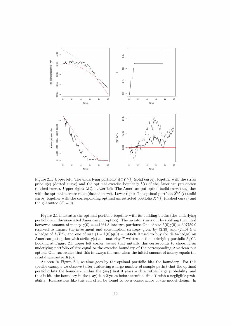
0 2 4 6 8 10

0e+0

01e

+05

2e+0

53e

+05

4e+0

5

Time

The

unco

nstra

ined

portf

olio

( λY

*)

0 2 4 6 8 10

0.70

0.75

0.80

0.85

Time

λ

0 2 4 6 8 10

020

000

4000

060

000

8000

010

0000

Time

Amer

ican

put−

optio

n va

lue

0 2 4 6 8 10

0e+0

05e

+04

1e+0

5

Time

OBPI

(V(λ)

)

Figure 2.1: Upper left: The underlying portfolio λ(t)Y ∗(t) (solid curve), together with the strikeprice g(t) (dotted curve) and the optimal exercise boundary b(t) of the American put option(dashed curve). Upper right: λ(t). Lower left: The American put option (solid curve) togetherwith the optimal exercise value (dashed curve). Lower right: The optimal portfolio X(λ)(t) (solidcurve) together with the corresponding optimal unrestricted portfolio X∗(t) (dashed curve) andthe guarantee (K = 0).

Figure 2.1 illustrates the optimal portfolio together with its building blocks (the underlyingportfolio and the associated American put option). The investor starts out by splitting the initialborrowed amount of money g(0) = 441361.8 into two portions: One of size λ(0)g(0) = 307759.9reserved to finance the investment and consumption strategy given by (2.39) and (2.40) (i.e.a hedge of λ0Y ∗), and one of size (1 − λ(0))g(0) = 133601.9 used to buy (or delta-hedge) anAmerican put option with strike g(t) and maturity T written on the underlying portfolio λ0Y ∗.Looking at Figure 2.1 upper left corner we see that initially this corresponds to choosing anunderlying portfolio of size equal to the exercise boundary of the corresponding American putoption. One can realize that this is always the case when the initial amount of money equals thecapital guarantee K(0).

As seen in Figure 2.1, as time goes by the optimal portfolio hits the boundary. For thisspecific example we observe (after evaluating a large number of sample paths) that the optimalportfolio hits the boundary within the (say) first 3 years with a rather large probability, andthat it hits the boundary in the (say) last 2 years before terminal time T with a negligible prob-ability. Realizations like this can often be found to be a consequence of the model design. In

30

this example the reason is partly due to the fact that the investor is endowed with an increasinglabor income and no initial wealth. Looking at the optimal consumption strategy (2.39) oneobserves that this labor income design causes the investor, who holds a small portfolio, to savea little fraction of the labor income in the beginning of the period, whereas he chooses to savea large fraction of the labor income in the years just before terminal time T (see Figure 2.2).

In Section 2.5.1 we found how to change λ dynamically in order for the put option basedstrategy to be admissible. In Figure 2.1 upper right corner we see how λ(t), t ∈ [0, T ], increaseswhen the underlying process (λY ∗)t∈[0,T ] hits the exercise boundary of the American put option.Consequently, the American put option never exceeds its inner value as seen in Figure 2.1 lowerleft corner.

Finally, Figure 2.1 lower right corner shows the optimal portfolio plotted against the corre-sponding unrestricted optimal portfolio. We see how the optimal portfolio stays above or at zeroduring the time period while the unrestricted optimal portfolio becomes negative over severaldistinct time intervals. The fact that the optimal portfolio increases drastically away from zerothe last two years before terminal time T is primary due to the fact that the investor’s optimalconsumption strategy leaves room for saving labor income in the final years whenever wealth issufficient low (see Figure 2.2).

0 2 4 6 8 10

020

000

4000

060

000

Time

Optim

al co

nsum

ption

rate

(c*)

Figure 2.2: The optimal consumption rate (solid curve) together with the optimal unrestrictedconsumption rate (dashed curve), the deterministic labor income rate (dotted curve) and thedeterministic optimal boundary consumption rate (solid smooth curve).

In Figure 2.2 we see how the optimal consumption rate fluctuates around the labor incomerate. To begin with it is optimal to save a certain fraction of the labor income. As invest-ments start to pay off it eventually becomes optimal to consume more than the labor income(t ∈ [2.5, 6.5]). After 6.5 years the investor loses money on his investments (for this specificsample path) and it therefore becomes optimal for him to start saving money again. One can

31

say that Figure 2.2 simply shows the investor’s preferences for consuming now versus consuminglater. Comparing to the optimal unrestricted consumption rate, we see that the restriction toborrow against future labor income has a smoothing effect on consumption (as shown by He andPagès (1993)). The reason that the optimal consumption rate at the boundary goes to zero isclear: As time approaches T while wealth is equal to zero it becomes infinitely valuable to savemoney since the marginal utility of terminal wealth goes to infinity as terminal wealth goes tozero.

0e+00 1e+05 2e+05 3e+05 4e+05

0.0e

+00

1.0e

−05

2.0e

−05

Terminal wealth

Den

sity

0 2 4 6 8 10

0.0

0.1

0.2

0.3

0.4

0.5

0.6

Time

Expo

sure

to s

tock

cha

nges

Figure 2.3: Upper window: The density of the optimal terminal wealth (solid curve) togetherwith the density of the optimal unrestricted terminal wealth (dashed curve). Vertical linesindicate the 95 percent confidence intervals. Lower window: The optimal fraction of totalwealth invested in the risky stock. The solid curve represents the median while the dashedcurves indicate the 95 percent confidence interval. The line y = 2

3 represents the unrestrictedoptimal fraction to invest in the risky stock.

In Figure 2.3 upper window we compare the optimal terminal wealth with the unrestrictedoptimal terminal wealth of Merton. Not surprisingly, the restriction to borrow against futurelabor income results in a much more narrow distribution for the terminal wealth. The optimalterminal wealth has 95 percent of its density mass within the interval [41854, 134252], whereasfor the unrestricted problem this interval is [32590, 169928]. Figure 2.3 lower window illustratesthe risk taken in the optimal portfolio. The risk taken is defined as the fraction of total wealth(wealth plus the financial value of future labor income) invested in the risky stock. We see thatthe median forms a ’s-curve’ towards the unrestricted Merton fraction

(π = 2

3

). This is due to

the fact that eventually, the optimal portfolio will increase away from the boundary (K = 0)and the American put option will become very cheap, resulting in a strategy almost identical tothe one of Merton. It should be stressed that we could easily find another example where thiswill not be the case. The very wide 95 percent confidence interval illustrates how the optimal

32

investment strategy can be very different for different sample paths. It also illustrates how muchthe optimal investment strategy differs from the unrestricted strategy of Merton. Even in thecase where the investor gets a very large and steady payoff from his risky investments he do notinvest nearly as aggressively as Merton before after 5 years (halfway). Reversely, in the case ofvery large and steady loses on the investments the investor places after 5 years only about 6percent of total wealth in the risky stock.

2.6 ConclusionWe have solved the classic consumption and investment control problem of Merton in the presenceof labor income and an American capital guarantee restriction. The solution obtained is anoption based portfolio insurance (OBPI) combining a long position in the optimal unrestrictedallocation with an American put option. More precisely, the investor optimally invests in abudget adjusted version of the unrestricted portfolio and buys an insurance on that portfolioin the form of an American put option. Initially the budget for the unrestricted portfolio isadjusted such that this is affordable. The introduction of consumption and labor income tosuch a setting is, to the author’s knowledge, not considered before, and the main contributionfrom this article was to show, by use of the martingale approach to arbitrage-free theory infinance, that the OBPI approach can be carried out to find the optimal strategy in the presenceof consumption and labor income. The introduction of a deterministic labor income by itself, inthe presence of an American capital guarantee, is not trivial. Unlike the unrestricted problem ofMerton, being endowed with a deterministic labor income or being endowed with an initial wealthenlarged by the financial value of future labor income is not equivalent. We have shown thatthe introduction of deterministic labor income can be handled by choosing an appropriate strikevalue for the American put option used to insure the investors portfolio from falling below thecapital restriction. The strategy, which has to be re-balanced whenever the constraint is active,is rather complicated. Another contribution offered by this article is an in-depth explanationand analysis of the optimal strategy supported by graphical illustrations.

33

34

3. Optimal consumption, investment andlife insurance with surrender optionguarantee

Abstract: We consider an investor, with an uncertain life time, endowed with deter-ministic labor income, who has the possibility to continuously invest in a Black-Scholesmarket and to buy life insurance or annuities. We solve the optimal consumption, in-vestment and life insurance problem when the investor is restricted to fulfill an Ameri-can capital guarantee. By allowing the guarantee to depend, in a very general way, onthe past we include, among other possibilities, the interesting case of a minimum rateof return guarantee, commonly offered by pension companies. The optimal strategiesturn out to be on option based portfolio insurance form, but since the capital guaran-tee is valid at every intermediate point in time, re-calibration is needed whenever theconstraint is active.

Keywords: Stochastic control; martingale method; life insurance; rate guarantee;option based portfolio insurance; CRRA utility.

3.1 IntroductionWe unify two directions of generalizing the classical Merton’s consumption-investment problemwith labor income, namely the introduction of life insurance decisions and the introduction ofcapital constraints. This unification is particularly relevant since the savings in a life and pensioncontract often contain restrictions that are special examples of our capital constraint. We solvethe joint problem where the individual with an uncertain life time can buy life insurance orannuities and, at the same time, there is a general capital constraint on his savings.

The uncertain life time is well-motivated but it turns a deterministic income rate while beingalive into a stochastic income rate. Access to life insurance and annuities completes the marketand makes the financial value of labor income unique.

The capital constraint allowed for in this paper is sufficiently general to cope with two well-motivated situations:

1) One possible capital constraint is that the savings are not allowed to become negative. Wecan speak of this as a no-borrowing constraint but it is important to stress that it is a constrainton wealth and not on investment position. In a life insurance context one would speak of sucha constraint as a non-negative reserve constraint. The intuition is that it should always be thepension institution that owes money to the policy holder and not the other way around. Thisis a standard institutional/regulatory constraint that serves to separate, institutionally, savingbusiness from lending business.

2) Another possible capital constraint is that the savings earn a minimum return. We speakof this as an interest rate guarantee. This is a delicate capital guarantee since it protects thedynamics of wealth rather than wealth itself. Thus, formalized as a constraint on the capitalitself, this constraint depends on the trajectory of the state variables. Such a guarantee appearsin many different types of life insurance contracts, ranging from participating life insurance witha so-called surrender option with a guaranteed sum upon surrender to unit-link life insurancewhere you can add on different types of options on the return.

In both situations one may ask why is the constraint there at all? The separation of saving

35

business from lending business perhaps serves to protect the pension institution from unspannedpolicy holder credit risk. We stress the word unspanned here because one could argue thatspanned life insurance risk is also credit risk in the context of borrowing against future income.Credit risk is a matter for the lending business who would require some material collateral, likea house or something, in addition to a ’planned’ working life. But there is no such unspannedpolicy holder credit risk within our model, so who asked for a constraint? Also the guarantee onreturn may seem odd: Who asked for that? The titular question posed by Jensen and Sørensen(2001) means almost the same. Well, the answer ’the social planner’ applies to both questions. Ifthe society prefers that savings are non-negative, or if the society prefers that policy holders (viatheir delegated pension institutions) invest as safely as it is dictated by an interest rate guarantee,then the constraints can appear through the regulatory environment. Thus, these constraintsshould not necessarily be interpreted as a twist on the policy holders preferences within themodel but as a societal constraint from outside the model/preferences. Formalistically, the twointerpretations are the same, though. It is interesting to discuss if and when such constraintsreally are meaningful from the point of view of the social planner. However, this is beyondthe scope of this paper. Furthermore, during these decades where certain markets show atendency from classical interest rate guarantee participating life insurance towards modern unit-link products, the policy holders tend to actually buy these options on the return. So, could it besomething that the people want, after all? Prospect theory may help motivating guarantees, seee.g. Døskeland and Nordahl (2008). We do not incorporate prospect theory in our preferencesbut take the guarantees to be exogenously given.

Life insurance was introduced to Merton’s classical consumption-investment problem firstalready by Richard (1975) but Yaari (1965) had even earlier results in discrete time. It took threedecades before the actuarial academic community realized the importance of the fundamentalpatterns of thinking by Richard (1975). Since then, many articles generalize the results byRichard in various directions. They include Pliska and Ye (2007) who allow for an unboundedlifetime; Huang and Milevsky (2008) who allow for unspanned labor income; Huang et al. (2008)who separate the breadwinner income process from the family consumption process; Steffensenand Kraft (2008) who generalize to a multistate Markov chain framework typically used byactuaries for modeling a series of life history events; Nielsen and Steffensen (2008) who workwith constraints on the insurance sum paid out upon death; Bruhn and Steffensen (2011) whogeneralize to a multiperson household, with focus on a married couple with economically and/orprobabilistically dependent members; Kwak et al. (2011) who also consider a household but focuson generation issues.

Our contribution compared to the list of papers in the former paragraph is that we addcapital constraints. They are particularly interesting since the life insurance and pension savingscontracts typically contain borrowing or return constraints set by either the insurance companydirectly or by the regulatory authorities indirectly.

Capital constraints have been studied in a series of papers. They were first studied as aEuropean (i.e. terminal) capital constraint in Teplá (2001) and Jensen and Sørensen (2001) who,interestingly, motivated the study of capital constraints from guarantees in pension contracts.Later results of El-Karoui et al. (2005) concern an American (i.e. continuous) capital guaranteed.The three papers on capital constraints mentioned above all deal with the investment problemexclusively, disregarding labor income and consumption. Kronborg (2011) generalizes the resultsof El-Karoui et al. (2005) to include spanned labor income and optimal consumption.

Our contribution compared to the list of papers in the former paragraph is that we addlife insurance risk and decisions and allow for more general path dependent constraints. Thiscombination makes it possible to study realistic decision processes and product designs includingrelevant regulatory and/or institutional constraints in the pension savings market.

Speaking of terminal and continuous constraints as being European and American, respec-tively, may seem a bit far-fetched until the resulting strategy appears: The best strategy is tofollow a so-called option based portfolio insurance strategy (OBPI) where a certain part of thecapital is invested in the optimal portfolio for the unconstrained problem and then put option

36

protected downwards for the residual amount such that the guarantee is fulfilled and such thatthe combined position is worth the wealth. In the European case the portfolio is protected by aEuropean put option whereas in the American case the portfolio is protected by an American putoption. The underlying portfolio of the American put option is continuously updated, though,paid by the cash flow from the put option, see El-Karoui et al. (2005). A particular feature arisesin the presence of income and consumption, namely, that also the strike is updated, see Kronborg(2011). This ’updating of the American strike’ pattern appears also in the present paper in thepresence of life insurance risk and protection. The update becomes even more delicate due tothe path dependence of the capital guarantee.

Two other lines of literature should be mentioned for dealing with related problems althoughthe market or the control fundamentally differ: Optimal annuitization has been studied in aseries of papers, see Milevsky and Young (2007) and references therein. Optimal retirementtiming has been studied in e.g. Farhia and Panageas (2007). We also wish to mention Dybvigand Liu (2010) since they combine the retirement decision with capital constraints similar to theones we deal with here.

We apply the martingale method developed by Cvitanic et al. (1987), Cox and Huang (1989),Cox and Huang (1991) and Cvitanic and Karatzas (1992). This method deals efficiently withcapital constraints and has been used in all the papers on capital constraints mentioned above.However, Kraft and Steffensen (2012) show how also dynamic programming applies to problemswith capital constraints.

The outline of the paper is as follows: In Section 2, we present the state processes and definethe natural set of admissible strategies in presence of spanned labor income. In Section 3, weformalize and solve the unconstrained problem. Section 4 contains a formalization and a solutionto the constrained problem. Numerical examples of the (constrained and unconstrained) optimalwealth dynamics are illustrated. We conclude in Section 5. Finally, a rigorous proof showingthe admissibility of the strategy found in Section 4 is presented in the appendix.

3.2 SetupConsider a policyholder with a life insurance policy issued at time 0 and terminated at a deter-ministic point in time 0 < T < ∞. One should think of T as the time of retirement decidedbeforehand by the policyholder. The policyholder’s time of death is given by a non-negativerandom variable τd defined on a given probability space (Ω,F , P ). We assume that τd has aprobability distribution given by a function F with density function denoted by f . We can thendefine the survivor function F by

F (t) := P (τd ≥ t) = 1− F (t) where F (t) := P (τd < t) =

∫ t

0

f(s)ds. (3.1)

The instantaneous time-t mortality rate of the policyholder is given by the hazard function

µ(t) := limϵ→0

P (t ≤ τd < t+ ϵ | τd ≥ t)

ϵ= lim

ϵ→0

F (t+ ϵ)− F (t)

ϵ

1

F (t)=F ′(t)

F (t)=f(t)

F (t)= − ∂

∂tlogF (t).

We get the following well-known expressions frequently used by actuaries

F (t) = e−∫ t0µ(s)ds, (3.2)

f(t) = µ(t)e−∫ t0µ(s)ds. (3.3)

In this paper we assume that the mortality rate is deterministic and given by a continuousfunction µ : [0,∞) → [0,∞).

We now describe the investment and life insurance market available to the policyholder.Consider a Black-Scholes market consisting of a bank account, B, with risk free short rate, r,

37

and a risky stock, S, with dynamics given by

dB(t) = rB(t)dt, B(0) = 1,

dS(t) = αS(t)dt+ σS(t)dW (t), S(0) = s0 > 0.

Here α, σ, r > 0 are constants and we assume α > r. The process W is a standard Brownianmotion on the probability space (Ω,F ,P) equipped with the filtration FW = (FW (t))t∈[0,T ]

given by the P -augmentation of the filtration σW (s); 0 ≤ s ≤ t,∀t ∈ [0, T ]. We assume thatthe policyholder’s random time of death τd is stochastically independent of the filtration FW .

The policyholder is assumed to be endowed with a continuous deterministic labor incomeof rate ℓ(t) ≥ 0,∀t ∈ [0, T ], as long as he is alive, and possibly an initial amount of moneyx0 ≥ 0. The policyholder should be thought of as an agent who has the possibility to invest andcontinuously consume from or save on a pension account. Naturally, we, as done by actuaries,refer to the policyholder’s wealth, denoted by X, as the reserve. The reserve is maintainedand invested by the pension company, but the policyholder chooses, in a continuous way, therisky asset allocation and the sum insured to be paid out upon death before time T 1. Morespecifically, let c ≥ 0 be the rate of consumption and let θ be the amount of money investedin the risky stock. Furthermore, let D ∈ [0,∞) be the sum insured to be paid out upon deathbefore time T . Choosing D, the policyholder agrees to hand over the amount of money X−D tothe pension company upon death before time T , i.e. the pension company keeps the reserve X forthemselves and pays out D as life insurance. Disregarding policy expenses the natural actuarialrisk premium rate to pay for the life insurance D at time t is µ(t)(D(t)−X(t))dt. Observe thatchoosing D > X corresponds to buying a life insurance and choosing D < X corresponds toselling a life insurance, i.e. buying an annuity. The dynamics of the reserve at the state alive2

becomes

dX(t) = [rX(t) + θ(t)(α− r) + ℓ(t)− c(t)− µ(t)(D(t)−X(t))]dt+ σθ(t)dW (t), t ∈ [0, T ),(3.4)

X(0) = x0.

Once again we stress that in the case of death before the terminal time T only the sum insured,D, is paid out to the policyholder. We call the cash flow injected to the reserve given byℓ(t)− c(t)− µ(t)D(t), ∀t ∈ [0, T ], the pension contributions.

We assume the trading strategy, θ, to be an FWt -adapted process with

∫ T

0(θ(t))2dt <∞ a.s.,

the consumption rate, c, to be a non-negative FWt -adapted process with

∫ T

0c(t)dt <∞ a.s., and

the insurance strategy, D, to be a non-negative FWt -adapted process with

∫ T

0D(t)dt < ∞ a.s.

Note that this ensures that X is well-defined and we get the unique solution, ∀t ∈ [0, T ], knownas the time-t retrospective reserve

X(t) = x0e∫ t0(r+µ(y))dy +

∫ t

0

e∫ ts(r+µ(y))dy[θ(s)(a− r) + ℓ(s)− c(s)− µ(s)D(s)]ds

+

∫ t

0

e∫ ts(r+µ(y))dyσθ(s)dW (s). (3.5)

It is well known that in the Black-Scholes market the equivalent martingale measure, Q, is uniqueand given by the Radon-Nikodym derivative

dQ(t)

dP (t)= Λ(t) := exp

(−∫ t

0

α− r

σdW (s)− 1

2

∫ t

0

(α− r

σ

)2

ds

), t ∈ [0, T ], (3.6)

1An alternative interpretation, also given by Nielsen and Steffensen (2008), is that the company chooses theinvestment and life insurance strategy on the behalf of the policyholder.

2For the rest of the paper we refer to the reserve at the state alive as simply the reserve.

38

and that the process WQ given by

WQ(t) =W (t) +α− r

σt, t ∈ [0, T ], (3.7)

is a standard Brownian motion under the martingale measure Q. We get that the time-t retro-spective reserve can be represented, ∀t ∈ [0, T ], by

X(t) = x0e∫ t0(r+µ(y))dy +

∫ t

0

e∫ ts(r+µ(y))dy[ℓ(s)− c(s)− µ(s)D(s)]ds

+

∫ t

0

e∫ ts(r+µ(y))dyσθ(s)dWQ(s). (3.8)

Definition 3.2.1. Define the set of admissible strategies, denoted by A, as the consumption,investment and life insurance strategies for which the corresponding wealth process given by (3.8)is well-defined,

X(t) + g(t) ≥ 0, ∀t ∈ [0, T ], (3.9)

where g is the time-t actuarial value of future labor income defined by

g(t) :=

∫ T

t

e−∫ st(r+µ(y))dyℓ(s)ds,

and

EQ

[∫ T

0

e−∫ s0(r+µ(y))dyσθ(s)dWQ(s)

]= 0. (3.10)

The technical condition (3.10) is equivalent to the condition that under Q the process∫ t

0

e−∫ s0(r+µ(y))dyσθ(s)dWQ(s), t ∈ [0, T ],

is a martingale (in general it it only a local martingale, and also a supermartingale if (3.9) isfulfilled, see e.g. Karatzas and Shreve (1998)). From this we conclude that (3.10) insures that(c, θ,D) ∈ A if and only if X(T ) ≥ 0 and, ∀t ∈ [0, T ],

X(t) + g(t) = EQ

[∫ T

t

e−∫ st(r+µ(y))dy(c(s) + µ(s)D(s))ds+ e−

∫ Tt

(r+µ(y))dyX(T )

∣∣∣∣∣ FW (t)

].

(3.11)

At time zero this means that the strategies have to fulfill the budget constraint

x0 + g(0) = EQ

[∫ T

0

e−∫ t0(r+µ(y))ds(c(t) + µ(t)D(t))dt+ e−

∫ T0

rdsX(T )

]. (3.12)

For latter use we state the following remark.

Remark 3.2.1. Define

Z(t) := −∫ t

0

e−∫ s0(r+µ(y))dy(ℓ(s)− c(s)− µ(s)D(s))ds+ e−

∫ t0(r+µ(y))dyX(t), t ∈ [0, T ]. (3.13)

By (3.8) we have that condition (3.10) is fulfilled if and only if Z is a martingale under Q.The natural interpretation is that under Q the discounted reserve minus the discounted pension

39

contributions should be a martingale. It is useful to note that if Z is a martingale under Q thedynamics of X can be represented in the form

dX(t) = [(r + µ(t))X(t) + ℓ(t)− c(t)− µ(t)D(t)]dt+ ϕ(t)dWQ(t), t ∈ (0, T ], (3.14)

for some FW (t)-adapted process ϕ. Moreover, if the dynamics of X can be represented in theform given by (3.14) for some FW (t)-adapted process ϕ satisfying ϕ(t) ∈ £2, ∀t ∈ [0, T ], thenZ is a martingale under Q.

Finally, by condition (3.9) we allow the reserve process to become negative, as long as it doesnot exceed (in absolute value) the actuarial value of future labor income. Note that condition(3.9) puts a lower boundary on the reserve process and therefore rules out doubling strategies(see e.g. Karatzas and Shreve (1998)).

3.3 The unrestricted pension problemFor the unrestricted pension problem the policyholder chooses his consumption, investment andlife insurance strategy in order to optimize the expected utility from consumption, bequest upondeath, and terminal pension. That is, he searches for the strategy fulfilling the supremum

sup(c,θ,D)∈A′

E

[∫ T∧τd

0

e−∫ t0β(s)dsu(c(t))dt+K1e

−∫ τd0 β(s)dsu(D(τd))1(τd<T )

+K2e−

∫ T0

β(s)dsu(X(T ))1(τd≥T )

], (3.15)

where u : R → [−∞,∞) is a utility function representing the policyholder’s risk aversion and βis a deterministic function representing the policyholder’s time preferences. The set A′, calledthe set of feasible strategies, is a subset of the admissible strategies, defined by

A′ :=

(c, θ,D) ∈ A

∣∣∣∣∣ E[∫ T∧τd

0

e−∫ t0β(s)ds min(0, u(c(t)))dt

+ e−∫ τd0 β(s)dsK1 min(0, u(D(τd)))1(τd<T ) + e−

∫ t0β(s)dsK2 min(0, u(X(T )))1(τd≥T )

]> −∞

.

(3.16)

We see that it is allowed to draw an infinite utility from a strategy (c, θ,D) ∈ A′, but only if theexpectation over the negative parts of the utility function is finite. Clearly, for a positive utilityfunction we have that A and A′ coincide. The constant weight factors K1 > 0 and K2 > 0 aremeasures of the policyholder’s preferences concerning life insurance versus immediate consump-tion, and terminal pension versus immediate consumption, respectively. The case K1 = 0 hasthe well-known solution given by the pioneering work of Merton (1971). The case K2 = 0 andthe case excluding consumption can be analyzed along the same lines as the analysis given inthis paper. In order not to complicate the analysis further this will not be done since it requiresspecial treatment. The results are given by natural modifications of the results obtained in thispaper.

We want to write the optimization problem (3.15) in terms of the policyholder’s instanta-neous mortality rate. By the assumption that the random time of death, τd, is stochasticallyindependent of the filtration FW , and by use of (3.1), we can rewrite the expectation in (3.15)

40

as

E

[1τd≥T

∫ T

0

e−∫ t0β(s)dsu(c(t))dt+ 1τd<T

∫ τd

0

e−∫ t0β(s)dsu(c(t))dt

+K1e−

∫ τd0 β(s)dsu(D(τd))1(τd<T ) +K2e

−∫ T0

β(s)dsu(X(T ))1(τd≥T )

]

= E

[F (T )

∫ T

0

e−∫ t0β(s)dsu(c(t))dt+

∫ T

0

f(y)

∫ y

0

e−∫ t0β(s)dsu(c(t))dtdy

+K1

∫ T

0

e−∫ t0β(s)dsu(D(t))f(t)dt+K2e

−∫ T0

β(s)dsu(X(T ))F (T )

]. (3.17)

Observe that∫ T

0

f(y)

∫ y

0

e−∫ t0β(s)dsu(c(t))dtdy =

∫ T

0

e−∫ t0β(s)dsu(c(t))

∫ T

t

f(y)dydt

=

∫ T

0

e−∫ t0β(s)dsu(c(t))

[F (t)− F (T )

]dt.

Plug this into (3.17) to obtain

E

[∫ T

0

e−∫ t0β(s)dsu(c(t))F (t)dt+K1

∫ T

0

e−∫ t0β(s)dsu(D(t))f(t)dt+K2e

−∫ T0

β(s)dsu(X(T ))F (T )

].

(3.18)

Finally, inserting (3.2) and (3.3) into (3.18) we can write the optimization problem (3.15) as

sup(c,θ,D)∈A′

E

[∫ T

0

e−∫ t0(β(s)+µ(s))ds[u(c(t)) +K1µ(t)u(D(t))]dt+K2e

−∫ T0

(β(s)+µ(s))dsu(X(T ))

].

(3.19)

For the rest of this paper we assume that the policyholder’s preferences towards risk are givenby a constant relative risk aversion function (CRRA) in the form

u(x) =

xγ

γ , if x > 0,

limx0xγ

γ , if x = 0,

−∞, if x < 0,

for some γ ∈ (−∞, 1)\0.

Remark 3.3.1. We conjecture that the analysis presented in this paper can be extended to thecase of a general utility function. This would, following the ideas of El-Karoui and Karatzas(1995) and El-Karoui et al. (2005), require use of the Gittins index methodology. We specialize tothe case of CRRA utility due to the well-known property that the maximization problem (3.15)becomes linear in initial total wealth. Even in the case of a general path dependent constrainton the reserve (see Section 3.4) this feature allows us to derive fairly explicit expressions forthe optimal strategies, leaving us with a greater understanding of the impact on the strategiescaused by the introduced constraints.

3.3.1 How to choose K2 - consumption after retirementChoosing K1 is really a matter of personal preferences. How much do you love yourself relativelyto your inheritors? However, choosing K2 can be done in a natural way. A common choice in

41

the literature of consumption/portfolio selection is K2 = 1 by simply not allowing any weightconstant. This corresponds to the case where the agent prefers a terminal wealth approximatelyequal to the size of accumulated consumption over the last year before the terminal time T . Atleast in a pension context this seems to be a very odd choose. What the policyholder (probably)wants is a terminal pension big enough for him to be able to maintain his standard of livingthroughout his uncertain remaining life time. At the same time, he should still take his timepreferences into account. Define therefore the actuarial time-T value of a life annuity paying 1per year continuously until the time of death as

a(T ) := E

[∫ ∞

T

e−∫ sTr dy1(τd≥s)ds

∣∣∣∣∣ τd > T

]=

∫ ∞

T

e−∫ sT(r+µ(y))dyds.

Disregarding policy expenses, the policyholder standing at the time of retirement, T , might usehis terminal pension X(T ) to buy, in the life insurance market, a life annuity of rate X(T )/a(T ).Assume that he chooses to do so and thereafter simply consumes the entire life annuity (leavingno room for saving)3. We get that

E

[∫ ∞

T

e−∫ s0β(y)dyu

(X(T )

a(T )

)1(τd≥s)ds

]= E

[∫ ∞

T

e−∫ s0(β(y)+µ(y))dyu

(X(T )

a(T )

)ds

]= E

[e−

∫ T0

(β(y)+µ(y))dy

∫ ∞

T

e−∫ sT(β(y)+µ(y))dydsu

(X(T )

a(T )

)]= E

[e−

∫ T0

(β(y)+µ(y))dyaS(T )u

(X(T )

a(T )

)], (3.20)

where

aS(T ) := E

[∫ ∞

T

e−∫ sTβ(y)dy1(τd≥s)ds

∣∣∣∣∣ τd > T

]=

∫ ∞

T

e−∫ sT(β(y)+µ(y))dyds

defines the subjective actuarial time-T value of a life annuity paying 1 per year continuouslyuntil the time of death. Comparing the terminal term in (3.19) with (3.20) we get the naturalchoice

K2 = aS(T )a(T )−γ . (3.21)

3.3.2 Solving the unrestricted problemWe now solve the unrestricted optimization problem given by (3.15). In the calculations we focuson the representation of the problem given by (3.19). The methodology used in the following,introduced by Cvitanic et al. (1987), Cox and Huang (1989), Cox and Huang (1991) and Cvi-tanic and Karatzas (1992), is know as the martingale method. One could, as done in Richard(1975), Pliska and Ye (2007), Nielsen and Steffensen (2008), Huang et al. (2008) and others,have used the Hamilton-Jacobi-Bellman (HJB) technique to derive the optimal consumption,investment and life insurance strategy. We choose the martingale approach since the solutionto the restricted capital guarantee problem introduced in Section 3.4 is based on terms derivedfrom the martingale method in the unrestricted case. Since the HJB technique seems to be theapproach applied in the literature to solve such unrestricted optimization problems as (3.15)this subsection may also serve, in its own right, as an example of how to apply the martingaleapproach to a classic continuous time unrestricted optimization problem including life insurance.First we state the result in Proposition 3.3.1. The result is also obtained, in slightly different

3The classical annuity result of Yaari (1965) proves that consuming the entire annuity income is optimal inthe absence of bequest.

42

forms due to different setups and notation, by e.g. Richard (1975), Pliska and Ye (2007) andNielsen and Steffensen (2008).

Proposition 3.3.1. The optimal strategy for the problem (3.15) is given by the feedback forms

c∗(t) :=X(t) + g(t)

f(t), (3.22)

D∗(t) :=X(t) + g(t)

f(t)K

11−γ

1 , (3.23)

θ∗(t) :=1

1− γ

α− r

σ2(X(t) + g(t)), (3.24)

where

g(t) :=

∫ T

t

e−∫ st(r+µ(y))dyℓ(s)ds, (3.25)

f(t) :=

∫ T

t

e−∫ st(r(y)+µ(y))dy

(1 + µ(s)K

11−γ

1

)ds+K

11−γ

2 e−∫ Tt

(r(y)+µ(y))dy, (3.26)

and

r(t) := − γ

1− γr − 1

2

γ

(1− γ)2

(α− r

σ

)2

+1

1− γβ(t). (3.27)

Proof. Let I : (0,∞] → [0,∞) denote the inverse of the derivative of the utility function u andobserve that by use of the concavity of u we have

u(x) ≤ u(I(z))− z(I(z)− x), ∀x ≥ 0, z > 0. (3.28)

Define the adjusted state price deflator H as

H(t) := Λ(t)e∫ t0(β(s)−r)ds,

and define ξ∗ > 0 as the constant satisfying

H(ξ∗) := EQ

[∫ T

0

e−∫ t0(r+µ(s))ds

[I(ξ∗H(t)) + µ(t)I

(K−1

1 ξ∗H(t))]dt

+ e−∫ T0

(r+µ(s))dsI(K−1

2 ξ∗H(T )) ]

= x0 + g(0). (3.29)

Such a ξ∗ clearly exist since I is continuous and decreasing and maps (0,∞] onto [0,∞) (see e.g.Karatzas and Shreve (1998), Chapter 3, Lemma 6.2).

Now, take an arbitrary strategy (c, θ,D) ∈ A′ with corresponding wealth process (X(t))t∈[0,T ]

as given. Using (3.28), the budget constraint (3.12) and finally (3.29) we get that

E

[∫ T

0

e−∫ t0(β(s)+µ(s))ds[u(c(t)) +K1µ(t)u(D(t))]dt+K2e

−∫ T0

(β(s)+µ(s))dsu(X(T ))

]

≤ E

[∫ T

0

e−∫ t0(β(s)+µ(s))ds[u(I(ξ∗H(t))) +K1µ(t)u(I(K

−11 ξ∗H(t)))]dt

+K2e−

∫ T0

(β(s)+µ(s))dsu(I(K−12 ξ∗H(T )))

].

43

Since (c, θ,D) was an arbitrarily chosen feasible strategy we obtain the candidate optimal strat-egy (c∗, θ∗, D∗) given by

c∗(t) = I(ξ∗H(t)), (3.30)

D∗(t) = I(K−11 ξ∗H(t)), (3.31)

X∗(T ) = I(K−12 ξ∗H(T )). (3.32)

We have expressed the candidate optimal investment strategy in terms of the optimal terminalpension given by (3.32). Since (c∗, θ∗, D∗), by the definition of ξ∗, fulfills the budget constraint(3.12) it is well known that, in a complete market, there exist an investment strategy θ∗ suchthat X(T ) = X∗(T ) and (c∗, θ∗, D∗) is admissible (see e.g. Cvitanic and Karatzas (1992) orKaratzas and Shreve (1998)). We are now going to calculate the hedging investment strategy θ∗and to write the expressions (3.30) and (3.31) in more explicit forms.

Observing that I(x) = x−1/(1−γ) we get from (3.29) that

H(ξ∗) = E

[∫ T

0

H(t)e−∫ t0(µ(s)+β(s))ds(ξ∗)

−11−γH(t)

−11−γ

(1 + µ(t)K

11−γ

1

)dt

+H(T )e−∫ T0

(µ(s)+β(s))dsK1

1−γ

2 (ξ∗)−11−γH(T )

−11−γ

]= (ξ∗)

−11−γ f(0),

where we have defined

f(t) = E

[∫ T

t

e−∫ st(µ(y)+β(y))dy

(H(s)

H(t)

) −γ1−γ

(1 + µ(s)K

11−γ

1

)ds

+ e−∫ Tt

(µ(y)+β(y))dyK1

1−γ

2

(H(T )

H(t)

) −γ1−γ

∣∣∣∣∣ FW (t)

]. (3.33)

Since H(ξ∗) = x0 + g(0) per definition, we get that

ξ∗ = (x0 + g(0))−(1−γ)f(0)1−γ .

Inserting this into (3.30)–(3.32) and using the budget constraint (3.12) we get the followingexpressions for the candidate optimal strategy

c∗(t) =X(t) + g(t)

f(t),

D∗(t) =X(t) + g(t)

f(t)K

11−γ

1 ,

X∗(T ) =X(t) + g(t)

f(t)

(H(T )

H(t)

) −11−γ

K1

1−γ

2 ,

and we recognize (3.22) and (3.23) from Proposition 3.3.1. To calculate f note that

E

[e−

∫ st(µ(y)+β(y))dy

(H(s)

H(t)

) −γ1−γ

∣∣∣∣∣ FW (t)

]= e

−∫ st

(µ(y)+ 1

1−γ β(y)− γ1−γ r− 1

2γ

(1−γ)2(α−r

σ )2)dy.

(3.34)

Now combine (3.33) and (3.34) to obtain

f(t) =

∫ T

t

e−∫ st[r(y)+µ(y)]dy

(1 + µ(s)K

11−γ

1

)ds+K

11−γ

2 e−∫ Tt

[r(y)+µ(y)]dy,

44

with r given by (3.27), which we identify as (3.26) from Proposition 3.3.1.From the Girsanov Theorem we have

dH(t) = H(t)

((β(t)− r)dt− α− r

σdW (t)

).

An application of Itô’s lemma gives that

dX∗(t) = . . . dt+ (X∗(t) + g(t))1

1− γ

α− r

σdW (t). (3.35)

If we compare (3.35) with the X-dynamics of the reserve given by (3.4) we get that

θ∗(t) =1

1− γ

α− r

σ2(X∗(t) + g(t)),

which we recognize as (3.24).Finally, plug in (3.22)–(3.24) into (3.4) to obtain

d(X∗(t) + g(t)) =

(r + µ(t) +

1

1− γ

(α− r

σ

)2

−(1 + µ(t)K

11−γ

1

)1

f(t)

)(X∗(t) + g(t))dt

+1

1− γ

α− r

σ(X∗(t) + g(t))dW (t). (3.36)

We get the solution

X∗(t) + g(t) = (x0 + g(0)) exp

∫ t

0

r + µ(s) +12 − γ

(1− γ)2

(α− r

σ

)2

− 1 + µ(s)K1

1−γ

1

f(s)

ds

+1

1− γ

α− r

σW (t)

. (3.37)

In particular, since f is bounded away from zero, ∀t ∈ [0, T ], we have that X∗(t), t ∈ [0, T ], iswell-defined, and clearly (3.9) is fulfilled. Moreover, since X∗ + g is lognormally distributed onecan easily show that

EQ

[∫ T

0

(θ∗)2dt

]<∞,

which ensures that (3.10) is fulfilled. We conclude that the candidate optimal strategy (c∗, D∗, θ∗)given by (3.22)–(3.24) is admissible. Since x0 and g(0) cannot both be zero we get, from (3.22),(3.23) and (3.37), that c∗(t), D∗(t) > 0, t ∈ [0, T ], and X∗(T ) > 0, and we note that theadditional condition (3.16) is fulfilled, i.e. (c∗, θ∗, D∗) is feasible. We conclude that (c∗, θ∗, D∗)is the optimal strategy for the unrestricted problem (3.15).

3.3.3 Comments on the unrestricted solutionThe function g defined by (3.25) is referred to as the actuarial present value of future laborincome. It is actuarial practice to define the reserve as a conditional expected present value offuture payments. Isolating X in (3.11) leaves us with such an expression for the reserve. Weget, ∀t ∈ [0, T ],

X(t) = EQ

[∫ T

t

e−∫ st(r+µ(y))dy(c(s)− ℓ(s) + µ(s)D(s))ds+ e−

∫ Tt

(r+µ(y))dyX(T )

∣∣∣∣∣ FW (t)

].

45

We call the sum of the reserve and the actuarial present value of future labor income, given by(3.37), the total reserve. By (3.24) we have that the optimal amount invested in the stock is,comparable to Merton (1971), proportional to the total reserve and to the Sharpe ratio of themarket, and dependent on the policyholder’s risk aversion. The optimal consumption rate andthe optimal life insurance strategy, given by (3.22) and (3.23), equals the total reserve dividedby the deterministic function f given by (3.26), and for the optimal life insurance, multipliedby the weight factor K1/(1−γ)

1 . The function f can be interpreted as a subjective value ofa unit consumption rate until terminal time T or time of death, whatever occurs first, plus asubjective actuarial present value of an endowment insurance paying K1/(1−γ)

1 upon death beforetime T and K

1/(1−γ)2 upon survival until time T . The value of f is subjective since the time

dependent function r given by (3.27), used for discounting in the expression of f , depends onthe policyholder’s risk aversion and time preferences. Naturally, we conclude that the optimalconsumption strategy is decreasing in K1 and K2. That is, a policyholder to whom bequestand/or terminal pension are more important will optimally consume less. We also observe, thata more impatient policyholder, i.e. a policyholder with a greater time preference parameter β,optimally consumes more and buys more life insurance than a less patient policyholder. Theoptimal consumption and life insurance strategy depends in a much more complex way on therisk aversion parameter γ. By use of (3.36) we get, as also obtained in Steffensen and Kraft(2008), that, ∀t ∈ [0, T ],

dc∗(t) =d(X∗(t) + g(t))

f(t)− X∗(t) + g(t)

f(t)2f ′(t)dt

=

(r − β(t) +

(α−rσ

)21− γ

+1

2

γ

(1− γ)2

(α− r

σ

)2)c∗(t)dt+

1

1− γ

α− r

σc∗(t)dW (t).

We get, ∀t ∈ [0, T ], the solutions

c∗(t) = c∗(0) exp

∫ t

0

(r − β(s) + 1

2

(α−rσ

)21− γ

)ds+

1

1− γ

α− r

σW (t)

,

D∗(t) = D∗(0) exp

∫ t

0

(r − β(s) + 1

2

(α−rσ

)21− γ

)ds+

1

1− γ

α− r

σW (t)

.

Note that c∗(t) and D∗(t) do not depend on µ(t). The optimal consumption and life insurancestrategy depend only on µ through f(0) and g(0) (through c∗(0) and D∗(0)), i.e. on the overalllevel of µ. Further discussions of the qualitative behavior of the optimal controls are found inPliska and Ye (2007).

3.4 The restricted pension problemFrom (3.37) we have for the unrestricted optimal solution that

X∗(t) > −g(t), ∀t ∈ [0, T ],

where g(t) is the time-t actuarial value of future labor income given by (3.25). Allowing for anegative reserve is in conflict with the usual constraint in life insurance that the reserve shouldbe non-negative at any time. This should be the case since, in practice, at any time the pol-icyholder holds the right to stop paying pension contributions. We say that the policyholderholds the right to surrender. This serves to separate, institutionally, the pension business fromthe lending business. For further discussion of this issue see the Introduction, Section 3.1. Aspointed out by Nielsen and Steffensen (2008), solving the unrestricted pension problem (3.15)we assume that the policyholder sticks to the pension contribution plan stipulated in the policy.

46

The interpretation is that in the unrestricted pension problem given by (3.15) the policyholderdecides initially on a consumption strategy, together with a life insurance strategy and an in-vestment strategy, and is thereafter obligated to follow that specific strategy, i.e. he does nothold the right to surrender at any time.

The purpose of this paper is to find the optimal consumption, investment and life insurancestrategy when the reserve is restricted to fulfill a capital guarantee at any point in time. Asdiscussed, a capital guarantee of size zero is simply motivated by the policyholder’s right tosurrender at any time during the saving period. Often pension companies offer a minimumconstant rate guarantee to the policyholders. In fact, such a guarantee is often found to bemandatory in compulsory (employer) pension schemes. In that case, the pension companyguarantees a minimum rate of return on all pension contributions. Of course, no pension companycan guarantee a constant minimum rate of return larger than the risk free short rate plus theobjective mortality rate4 since such a guarantee cannot be fulfilled with certainty. To cover ahole class of capital guarantee problems, including the two cases discussed, we allow the capitalguarantee restriction to depend on the past in a very general way. Note that since future pensioncontributions may be stochastic, the future capital guarantee may becomes stochastic. For acomprehensive discussion and motivation of the problem see the Introduction, Section 3.1. Morespecific, consider the problem given by the indirect utility function

sup(c,θ,D)∈A′

E

[∫ T

0

e−∫ t0(β(s)+µ(s))ds

(u(c(t)) +K1µ(t)u(D(t))

)dt+K2e

−∫ T0

(β(s)+µ(s))dsu(X(T ))

],

(3.38)

under the capital guarantee restriction

X(t) ≥ k(t, Z(t)), ∀t ∈ [0, T ], (3.39)

where Z(t) :=∫ t

0h(s,X(s))ds, and k and h are deterministic functions. The two guarantees

discussed above are covered by

k(t, z) = 0, (3.40)

and

k(t, z) = x0e∫ t0 (r

(g)+µ(s))ds + e∫ t0 (r

(g)+µ(s))dsz, (3.41)

with h(s, x) = e−∫ s0 (r

(g)+µ(y))dy (ℓ(s)− c(s, x)− µ(s)D(s, x)), where r(g) ≤ r is the minimumrate of return guarantee excess of the objective mortality rate µ. Note that we in the expressionof h have indicated the possible x dependence in the consumption and life insurance strategy.We can write (3.41) as

k(t, Z(t)) = x0e∫ t0 (r

(g)+µ(y))dy +

∫ t

0

e∫ ts (r

(g)+µ(y))dy [ℓ(s)− c(s)− µ(s)D(s)] ds. (3.42)

To clarify things, one could preferably compare (3.42) with the retrospective reserve expressiongiven by (3.5).

The solution to the restricted capital guarantee problem given by (3.38) and (3.39) turns outto be of the Option Based Portfolio Insurance (OBPI) form. OBPI strategies are also obtainedin El-Karoui et al. (2005) and Kronborg (2011), and for a European capital constraint in Teplá(2001). The big differences, compared to El-Karoui et al. (2005) and Kronborg (2011), are the

4Remember that the mortality rate is given by a deterministic function, i.e. the pension company has no riskconcerning life times.

47

introduction of life insurance and the possible stochastic capital guarantee restriction. In addi-tion, El-Karoui et al. (2005) does not include consumption and labor income. Combining classicresults from the American option theory in a Black-Scholes market and the OBPI constructiontechnique we are able to solve the restricted optimization problem given by (3.38) and (3.39).

Before we present the results we need some notation: Still, denote by X∗, c∗, θ∗ and D∗

the optimal unrestricted reserve and the unrestricted optimal consumption, investment and lifeinsurance strategy derived in Subsection 3.3.2, respectively. Let Y ∗(t) := X∗(t) + g(t) denotethe optimal unrestricted total reserve. By (3.36) and (3.7) we have that

dY ∗(t) =

(r + µ(t)−

(1 + µ(t)K

11−γ

1

)1

f(t)

)Y ∗(t)dt+

1

1− γ

α− r

σY ∗(t)dWQ(t), t ∈ (0, T ),

(3.43)

Y ∗(0) = y0,

where y0 := x0 + g(0). Denote by P ay,z(t, T, k + g) the time-t value of an American put option

with strike price k(s, Z(s)) + g(s),∀s ∈ [t, T ], where Z(t) = z, and maturity T written on aportfolio Y , where Y is the solution to (3.43) which equals y at time t. By definition the priceof such a put option is given, ∀t ∈ [0, T ], by

P ay,z(t, T, k + g) := sup

τ∈Tt,T

EQ[e−

∫ τt(r+µ(s))ds(k(τ, Z(τ)) + g(τ)− Y (τ))+

∣∣∣ Y (t) = y, Z(t) = z],

where Tt,T is the set of stopping times taking values in the interval [t, T ].

Theorem 3.4.1. Consider the strategy(c, θ, D

)given by, ∀t ∈ [0, T ],

c(t) := λ(t, Z(t))c∗(t) =λ(t, Z(t))Y ∗(t)

f(t), (3.44)

D(t) := λ(t, Z(t))D∗(t) =λ(t, Z(t))Y ∗(t)

f(t)K

11−γ

1 , (3.45)

θ(t) := λ(t, Z(t))θ∗(t) =1

1− γ

α− r

σ2λ(t, Z(t))Y ∗(t), (3.46)

combined with a position in an American put option written on the portfolio (λ(t)Y ∗(t))s∈[t,T ]

with strike price k(s, Z(s)) + g(s),∀s ∈ [t, T ], and maturity T . Here λ is the increasing functiondefined by

λ(t, Z(t)) = λ(0, z0) ∨ sups≤t

(b(s, Z(s))

Y ∗(s)

), (3.47)

with λ(0, z0) determined by

λ(0, z0)(x0 + g(0)) + P aλ(0,z0)y0,z0

(0, T, k + g)− g(0) = x0, (3.48)

and b being the optimal exercise boundary for the American put option given by

b(t, z) := supy : P a

y,z(t, T, k + g) = (k(t, z) + g(t)− y)+. (3.49)

We have that

• The strategy is optimal for the restricted capital guarantee problem given by (3.38) and(3.39).

48

Remark 3.4.1. By (3.37) the optimal unrestricted total reserve, Y ∗, is proportional to theinitial total reserve y0. Recall also that the optimal unrestricted consumption, life insuranceand investment strategy, given by (3.22)–(3.24), are proportional to the total reserve. It shouldthen be clear that starting out with reduced initial total reserve equal to λ(0, z0)(x0 + g(0))

and following the strategy (c, θ, D) given by (3.44)–(3.49) results in a total reserve equal toλ(t, Z(t))Y ∗(t),∀t ∈ [0, T ]. In total we get that the optimal restricted reserve becomes

X(λ)(t) := λ(t, Z(t))Y ∗(t) + P aλY ∗,Z(t, T, k + g)− g(t), t ∈ [0, T ], (3.50)

i.e. the optimal restricted reserve consists of a portfolio, an insurance on that portfolio and aloan equal to the actuarial value of future labor income.

Remark 3.4.2. The specific American put option is likely not to be sold in the market, butsince the market is complete and frictionless such options can be replicated dynamically by aDelta-hedge, i.e. the optimal investment strategy can be written as

θ(t) =

(1 +

∂

∂yP aλY ∗,Z(t, T, k + g)

)θ. (3.51)

Since the put option has an opposite exposure to changes in the underlying portfolio(λ(t)Y ∗(t))t∈[0,T ] we note that the total amount of money to invest in the risky asset, S, becomessmaller when we introduce an American capital guarantee to the control problem (3.15). Oneshould notice, that at the boundary no risk is taken, i.e. the position in the American put optionoffsets the position in the underlying portfolio such that the total exposure to changes in therisky asset, S, becomes zero. Clearly, at the boundary it is optimal to consume a certain time-dependent part of the labor income, thereby leaving room for a risky position in S immediatelyafter hitting the capital boundary.

Proof of Theorem 3.4.1. First, one should check that the strategy defined by Theorem 3.4.1fulfills the capital guarantee restriction given by (3.39). Using that the value of an Americanput option is always greater than or equal to its inner value this is easily done. We get

X(λ)(t) := λ(t, Z(t))Y ∗(t) + P aλY ∗,Z(t, T, k + g)− g(t)

≥ λ(t, Z(t))Y ∗(t) + [k(t, Z(t)) + g(t)− λ(t, Z(t))Y ∗(t)]+ − g(t)

≥ k(t, Z(t)), (3.52)

Second, one should check that the strategy defined by Theorem 3.4.1 is admissible. It turnsout that the rather complex strategy

(c, D, X(λ)

)involving the stochastic increasing function λ

is the natural way to make the OBPI admissible. The heuristic argument is as follows. Considerthe strategy

(c, D,X(λ)

)where λ(t, Z(t)) = λ0,∀t ∈ [0, T ], i.e. where we do not adjust λ. By

(3.52) such a strategy clearly fulfills the capital guarantee restriction. The strategy correspondsto, in addition to follow the consumption, life insurance and investment strategy given by (3.44)–(3.46), to hold the initially bought American put option to maturity. In some scenarios this is tothrow away money since the American put option is not sold when it is optimal to do so, i.e. thestrategy is not admissible (self-financing). The complicated strategy defined in Theorem 3.4.1is exactly designed to avoid this. The function λ defined by (3.47) and (3.48) correspondsto selling the American put option and re-balancing the strategy whenever optimal to do so.For a comprehensive explanation of the nature of the OBPI strategies see Kronborg (2011). Arigorous proof showing that the strategy in Theorem 3.4.1 is admissible is given in Appendix 3.6.

To prove the optimality of the strategy given in Theorem 3.4.1 we consider an arbitrar-ily chosen feasible strategy (c, θ,D) with corresponding reserve process (X(t)t∈[0,T ]) satisfying

49

X(0) = x0 and X(t) ≥ k(t, Z(t)),∀t ∈ [0, T ]. Since u is a concave function we get that∫ T

0

e−∫ t0(β(s)+µ(s))ds [u(c(t)) +K1µ(t)u(D(t))] dt+K2e

−∫ T0

(β(s)+µ(s))dsu(X(T ))

−

(∫ T

0

e−∫ t0(β(s)+µ(s))ds

[u(c(t)) +K1µ(t)u

(D(t)

)]dt+K2e

−∫ T0

(β(s)+µ(s))dsu(X(λ)(T )

))

=

∫ T

0

e−∫ t0(β(s)+µ(s))ds

[u(c(t))− u(c(t)) +K1µ(t)

(u(D(t))− u

(D(t)

))]dt

+K2e−

∫ T0

(β(s)+µ(s))ds(u(X(T ))− u

(X(λ)(T )

))≤∫ T

0

e−∫ t0(β(s)+µ(s))ds

[u′(c(t))(c(t)− c(t)) +K1µ(t)u

′(D(t)

)(D(t)− D(t)

)]dt

+K2e−

∫ T0

(β(s)+µ(s))dsu′(X(λ)(T )

)(X(T )− X(λ)(T )

)=: (∗). (3.53)

Since (c, θ,D) was arbitrarily chosen we simply end the proof by showing that E[(∗)] ≤ 0. Bythe CRRA property u′(xy) = u′(x)u′(y) we have

u′(c(t))(c(t)− c(t)) = u′(λ(t, Z(t)))u′(c∗(t))(c(t)− c(t)), (3.54)

u′(D(t)

)(D(t)− D(t)

)= u′(λ(t, Z(t)))u′(D∗(t))

(D(t)− D(t)

). (3.55)

Observe that since Y ∗(T ) = X∗(T ) the value of the terminal capital pension becomes

X(λ)(T ) = λ(T,Z(T ))X∗(T ) + [k(T,Z(T ))− λ(T,Z(T ))X∗(T )]+

= max[λ(T,Z(T ))X∗(T ), k(T,Z(T ))]. (3.56)

By use of (3.56) and using that u′ is a decreasing function we get that

u′(X(λ)(T )

)(X(T )− X(λ)(T )

)= min[u′(λ(T,Z(T )))u′(X∗(T )), u′(k(T,Z(T )))]

(X(T )− X(λ)(T )

)= u′(λ(T,Z(T )))u′(X∗(T ))

(X(T )− X(λ)(T )

)− [u′(λ(T,Z(T )))u′(X∗(T ))− u′(k(T ), Z(T ))]+ (X(T )− k(T,Z(T ))) ,

where the last equality is established by using that X(λ)(T ) = k(T,Z(T )) on the set(T, ω) : u′(λ(T,Z(T ))X∗(T )) ≥ u′(k(T,Z(T ))). Since by assumption X(t) ≥ k(t, Z(t)),∀t ∈[0, T ], we conclude that

u′(X(λ)(T )

)(X(T )− X(λ)(T )

)≤ u′(λ(T,Z(T )))u′(X∗(T ))

(X(T )− X(λ)(T )

). (3.57)

50

Now insert (3.54), (3.55) and (3.57) and then (3.30)–(3.32) into (3.53) to get

E[(∗)] ≤ E

[∫ T

0

e−∫ t0(β(s)+µ(s))ds

[u′(λ(t, Z(t)))u′(c∗(t)) (c(t)− c(t))

+K1µ(t)u′(λ(t, Z(t)))u′(D∗(t))

(D(t)− D(t)

) ]dt

+K2e−

∫ T0

(β(s)+µ(s))dsu′(λ(T,Z(T )))u′(X∗(T ))(X(T )− X(λ)(T )

)]

= ξ∗EQ

[∫ T

0

e−∫ t0(r+µ(s))dsu′(λ(t, Z(t)))

((c(t)− c(t)) + µ(t)

(D(t)− D(t)

))dt

+ e−∫ T0

(r+µ(s))dsu′(λ(T,Z(T )))(X(T )− X(λ)(T )

)].

Since u′(λ(t, Z(t))) is a decreasing function5 we can use the integration by parts formula to get

E[(∗)] ≤ ξ∗

(EQ

[∫ T

0

e−∫ t0(r+µ(s))dsu′(λ(t, Z(t)))

((c(t)− c(t)) + µ(t)

(D(t)− D(t)

))dt︸ ︷︷ ︸

(⋆)

+

∫ T

0

u′(λ(t, Z(t)))d(e−

∫ t0(r+µ(s))ds

(X(t)− X(λ)(t)

))︸ ︷︷ ︸

(⋆⋆)

]

+ EQ

[∫ T

0

e−∫ t0(r+µ(s))ds

(X(t)− X(λ)(t)

)du′(λ(t, Z(t)))︸ ︷︷ ︸

(⋆⋆⋆)

]). (3.58)

The third term in (3.58) can be rewritten as

EQ[(⋆ ⋆ ⋆)] = EQ

[∫ T

0

e−∫ t0(r+µ(s))ds(X(t)− k(t, Z(t)))du′(λ(t, Z(t)))

]

+ EQ

[∫ T

0

e−∫ t0(r+µ(s))ds

(k(t, Z(t))− X(λ)(t)

)du′(λ(t, Z(t)))

].

The first term is non-positive since per definitionX(t) ≥ k(t, Z(t)),∀t ∈ [0, T ], and du′(λ(t, Z(t))) ≤0,∀t ∈ [0, T ] (u′ is decreasing and λ is increasing). The second term equals zero since du′(λ(t, Z(t))) =0 only on the set (t, ω) : X(λ)(t) = k(t, Z(t)). We conclude that EQ[(⋆ ⋆ ⋆)] ≤ 0. The two firstterms of (3.58) can be rewritten as

EQ[(⋆) + (⋆⋆)] = EQ

[∫ T

0

u′(λ(t, Z(t)))dM1(t)

]− EQ

[∫ T

0

u′(λ(t, Z(t)))dM2(t)

], (3.59)

where

M1(t) :=

∫ t

0

e−∫ s0(r+µ(y))dy(c(s) + µ(s)D(s)− ℓ(s))ds+ e−

∫ t0(r+µ(y))dyX(t),

M2(t) :=

∫ t

0

e−∫ s0(r+µ(y))dy

(c(s) + µ(s)D(s)− ℓ(s)

)ds+ e−

∫ t0(r+µ(y))dyX(λ)(t).

5This ensures the that the stochastic integral in (3.58) is well-defined.

51

Since both strategies are admissible we have by (3.13) that M1 and M2 are martingales underthe equivalent measure Q. Since u′(λ(t, Z(t))) ≤ u′(λ(0, z0),∀t ∈ [0, T ], we get that

EQ[(⋆) + (⋆⋆)] = 0.

Finally, we can conclude that

E[(∗)] = EQ[(⋆) + (⋆⋆)] + EQ[(⋆ ⋆ ⋆)] ≤ 0.

3.4.1 Numerical illustrationsIn this subsection we illustrate the optimal strategy presented in Theorem 3.4.1 for the case of aminimum rate of return guarantee given by (3.42) with r(g) = 1

2r. The parameter values used forthe simulations are, for the Black-Scholes market, r = 0.01885, α = 0.05885 and σ = 0.2. Therather low risk free short rate and expected stock rate return should be interpreted as inflationadjusted parameters (subtracted 2.115 percent which is the average inflation in Denmark overthe last 20 years). Adjusting for inflation allow us to directly compare the size of the terminalpension with past reserve values and labor income. The personal preference towards risk is set toγ = −4 which is in accordance with the popular choice to have 20 percent of the reserve investedin stocks after retirement (we have 1

1−γα−rσ2 = 0.2). The time preference is set to the natural

value β = r, but one could of cause equally well had chosen the time preference parameter to besmaller or greater than the risk free short rate. However, it seems natural to have β ≥ r since thisassures that one cannot, in a risk free way, obtain a greater amount of utility by simply investingin the risk free short rate and then consume at a later point in time. Finally, we have chosen tomodel the uncertain life time by a Gompertz-Makeham hazard rate, u(x) = exp((x −m)/b)/b,with modal value and scale parameter as in Milevsky and Young (2007); (m, b) = (88.18, 10.5).

The individual we consider has just turned 50 years old, has a reserve of size 200000 euroand a constant future labor income of ℓ(t) = 30000, t ∈ [50, T ], with terminal time T = 65.The weight factor K2 in (3.38) is calculated by use of (3.21), but since it seems natural that thereserve will also be invested after retirement we have chosen to use r = 0.2α + 0.8r = 0.02685(since 1

1−γα−rσ2 = 0.2) for discounting in the expression of a(T ). The weight factor K1 in (3.38)

is set to K1 =∫ 10

0e−

∫ t+xt

β(y)dydx(b(10))−γ

with b(10)

=∫ 10

0e−

∫ s0rdyds. One can realize that

this is in accordance with the standard Danish choice of a 10 years period certain pension to theinheritor starting at the time of death (if death occurs before terminal time T ).

The remaining 15 years of optimization has been discretizied equidistantly into quarterlytime points, i.e. into 60 time points. By this we mean that the guarantee is only valid quarterlyand the American put option has been evaluated as a Bermuda put option with quarterly ex-ercise dates. Likewise, λ and therefore the optimal consumption, investment and life insurancestrategy has only been changed quarterly. Saying that, it is important to stress that betweenthe quarterly time points, consumption, investments and bequest have been re-balanced contin-uously6.

It seems natural to compare the restricted solution with the unrestricted counterpart. Fig-ure 3.1 illustrates how the restricted optimal reserve always is greater or equal to the guaranteewhile the unrestricted reserve sometimes is greater and sometimes smaller than the ’fictive’ guar-antee7. In fact we conclude that ignoring a guarantee requirement, and behaving optimal fromthe no guarantee point of view, will very likely result in a reserve smaller than the guarantee.

6We have used (3.37).7To be clear, there is of cause no guarantee belonging to the unrestricted reserve, but we can calculate the

guarantee anyway and then compare the unrestricted reserve with the guarantee.

52

Note that the restricted strategy can, for certain outcomes, outperform the unrestricted strat-egy both in terms of accumulated utility and terminal pension. In fact we have a 24 percentprobability that the restricted investor will obtain more utility over the interval of optimizationthan the unrestricted investor.

50 55 60 65

1500

0020

0000

2500

0030

0000

3500

0040

0000

4500

00

Age

Rese

rve

50 55 60 65

1500

0020

0000

2500

0030

0000

3500

0040

0000

4500

00

Age

Rese

rve

50 55 60 65

1500

0020

0000

2500

0030

0000

3500

0040

0000

4500

00

Age

Rese

rve

50 55 60 65

1500

0020

0000

2500

0030

0000

3500

0040

0000

4500

00

Age

Rese

rve

50 55 60 65

1500

0020

0000

2500

0030

0000

3500

0040

0000

4500

00

Age

Rese

rve

50 55 60 65

1500

0020

0000

2500

0030

0000

3500

0040

0000

4500

00

Age

Rese

rve

Figure 3.1: The restricted reserve (solid curves) and the unrestricted reserve (dashed curves)together with the corresponding guarantee (solid smooth curves) and fictive guarantee (dashedsmooth curves), respectively. The lower right plot indicates the average scenario.

In Table 3.1 we see that the restricted optimal terminal pension has a slightly smaller me-dian than the unrestricted one, but at the same time the restricted terminal pension has a muchmore narrow distribution. We also see that the pension saver with the minimum rate of re-turn guarantee will, in contrast to the one without, more or less avoid ending up with a verysmall terminal pension. We want to stress that one cannot use Table 3.1 to compare the perfor-mances of two strategies since money spent before the terminal time T is not taking into account.

The actuarial value of future labor income is g(50) = 380387 euro leaving the 50 years oldinvestor with a total reserve of size Y (50) = 580387. By simulation we calculate λ(50) = 0.9041meaning that initially about 90 percent of the total reserve is invested in the optimal unrestrictedportfolio and the remaining 10 percent is used to buy the American put option as an insuranceagainst downfalls in the portfolio. Figure 3.2 shows how lambda increases at the time pointswhere the insurance is in use (where it is optimal to sell the put option and re-calibrate theOBPI strategy accordingly to the new lambda value).

53

Fractal 0.001% 0.01% 2.5% 25% median 75% 97.5% 99.99 % 99.999%Restricted 10.21 10.58 11.33 12.18 13.12 14.30 17.08 22.03 23.60Unrestricted 6.10 7.53 10.02 12.22 13.57 15.09 18.39 24.09 25.91

Table 3.1: Reserve at retirement expressed in numbers of yearly labor income (the terminalreserve divided by the labor income rate). Chosen fractals for both the restricted and unrestrictedcase are presented.

50 55 60 65

0.905

0.910

0.915

Age

λ

50 55 60 65

0.90

0.95

1.00

1.05

Age

λ

50 55 60 65

0.90

0.95

1.00

1.05

1.10

1.15

Ageλ

50 55 60 65

0.92

0.94

0.96

0.98

Age

λ

50 55 60 65

0.904

20.9

044

0.904

60.9

048

0.905

00.9

052

Age

λ

Figure 3.2: The lambda process corresponding to the reserve processes from Figure 3.1.

The optimal investment strategy is given by (3.51) and (3.46). Figure 3.3 shows the optimalfraction of the total reserve invested in stocks. The main observation to do is to note howwide the 95 percent confidence interval is. Even in the case of very big investment returns ittakes about seven years (about half the optimization interval) before the insurance part becomesnegligible and the restricted investor starts to invest (almost) as aggressively as the unrestrictedinvestor. In the case of very low investment returns we see that the restricted investor getsstocked with the guarantee and cannot afford to take very much risk.

54

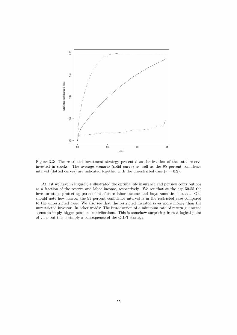
50 55 60 65

0.00

0.05

0.10

0.15

0.20

Age

Frac

tion

of to

tal w

ealth

to in

vest

in sto

cks

Figure 3.3: The restricted investment strategy presented as the fraction of the total reserveinvested in stocks. The average scenario (solid curve) as well as the 95 percent confidenceinterval (dotted curves) are indicated together with the unrestricted case (π = 0.2).

At last we have in Figure 3.4 illustrated the optimal life insurance and pension contributionsas a fraction of the reserve and labor income, respectively. We see that at the age 50-55 theinvestor stops protecting parts of his future labor income and buys annuities instead. Oneshould note how narrow the 95 percent confidence interval is in the restricted case comparedto the unrestricted case. We also see that the restricted investor saves more money than theunrestricted investor. In other words: The introduction of a minimum rate of return guaranteeseems to imply bigger pensions contributions. This is somehow surprising from a logical pointof view but this is simply a consequence of the OBPI strategy.

55

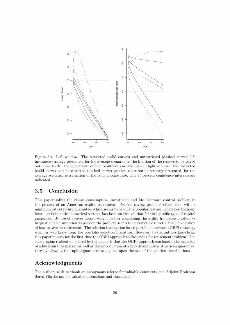
50 55 60 65

0.6

0.7

0.8

0.9

1.0

1.1

1.2

Age

Bequ

est /

Res

erve

50 55 60 65

−0.3

−0.2

−0.1

0.0

0.1

0.2

0.3

Age

Pens

ion co

ntrib

ution

/ La

bor in

come

Figure 3.4: Left window: The restricted (solid curves) and unrestricted (dashed curves) lifeinsurance strategy presented, for the average scenario, as the fraction of the reserve to be payedout upon death. The 95 percent confidence intervals are indicated. Right window: The restricted(solid curve) and unrestricted (dashed curve) pension contribution strategy presented, for theaverage scenario, as a fraction of the labor income rate. The 95 percent confidence intervals areindicated.

3.5 ConclusionThis paper solves the classic consumption, investment and life insurance control problem inthe present of an American capital guarantee. Pension saving products often come with aminimum rate of return guarantee, which seems to be quiet a popular feature. Therefore the mainfocus, and the entire numerical section, has been on the solution for this specific type of capitalguarantee. By use of cleaver chosen weight factors concerning the utility from consumption vsbequest and consumption vs pension the problem seems to be rather close to the real life questionof how to save for retirement. The solution is an option based portfolio insurance (OBPI) strategywhich is well know from the portfolio selection literature. However, to the authors knowledgethis paper applies for the first time the OBPI approach to the saving for retirement problem. Theencouraging realization offered by this paper is that the OBPI approach can handle the inclusionof a life insurance market as well as the introduction of a non-deterministic American guarantee,thereby allowing the capital guarantee to depend upon the size of the pension contributions.

AcknowledgmentsThe authors wish to thank an anonymous referee for valuable comments and Adjoint ProfessorSøren Fiig Jarner for valuable discussions and comments.

56

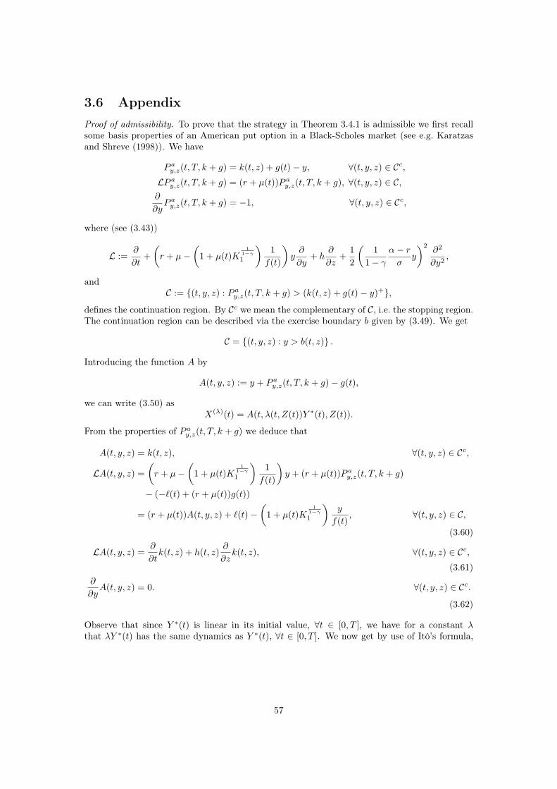
3.6 AppendixProof of admissibility. To prove that the strategy in Theorem 3.4.1 is admissible we first recallsome basis properties of an American put option in a Black-Scholes market (see e.g. Karatzasand Shreve (1998)). We have

P ay,z(t, T, k + g) = k(t, z) + g(t)− y, ∀(t, y, z) ∈ Cc,

LP ay,z(t, T, k + g) = (r + µ(t))P a

y,z(t, T, k + g), ∀(t, y, z) ∈ C,∂

∂yP ay,z(t, T, k + g) = −1, ∀(t, y, z) ∈ Cc,

where (see (3.43))

L :=∂

∂t+

(r + µ−

(1 + µ(t)K

11−γ

1

)1

f(t)

)y∂

∂y+ h

∂

∂z+

1

2

(1

1− γ

α− r

σy

)2∂2

∂y2,

andC := (t, y, z) : P a

y,z(t, T, k + g) > (k(t, z) + g(t)− y)+,

defines the continuation region. By Cc we mean the complementary of C, i.e. the stopping region.The continuation region can be described via the exercise boundary b given by (3.49). We get

C = (t, y, z) : y > b(t, z) .

Introducing the function A by

A(t, y, z) := y + P ay,z(t, T, k + g)− g(t),

we can write (3.50) asX(λ)(t) = A(t, λ(t, Z(t))Y ∗(t), Z(t)).

From the properties of P ay,z(t, T, k + g) we deduce that

A(t, y, z) = k(t, z), ∀(t, y, z) ∈ Cc,

LA(t, y, z) =(r + µ−

(1 + µ(t)K

11−γ

1

)1

f(t)

)y + (r + µ(t))P a

y,z(t, T, k + g)

− (−ℓ(t) + (r + µ(t))g(t))

= (r + µ(t))A(t, y, z) + ℓ(t)−(1 + µ(t)K

11−γ

1

)y

f(t), ∀(t, y, z) ∈ C,

(3.60)

LA(t, y, z) = ∂

∂tk(t, z) + h(t, z)

∂

∂zk(t, z), ∀(t, y, z) ∈ Cc,

(3.61)∂

∂yA(t, y, z) = 0. ∀(t, y, z) ∈ Cc.

(3.62)

Observe that since Y ∗(t) is linear in its initial value, ∀t ∈ [0, T ], we have for a constant λthat λY ∗(t) has the same dynamics as Y ∗(t), ∀t ∈ [0, T ]. We now get by use of Itô’s formula,

57

(3.60)–(3.61), (3.22)–(3.24), and the fact that λ increases only at the boundary, that8

dA(t, λ(t, Z(t))Y ∗(t), Z(t))

= [dA(t, λY ∗(t), Z(t))]|λ=λ(t,Z(t)) + Y ∗(t)∂

∂yA(t, λ(t, Z(t))Y ∗(t), Z(t))dλ(t, Z(t))

= λ(t, Z(t))∂

∂yA(t, λ(t, Z(t))Y ∗(t), Z(t))σθ∗(t)dWQ(t)

+[(r + µ(t))A(t, λ(t, Z(t))Y ∗(t), Z(t))

+ ℓ(t)− λ(t, Z(t))c∗(t)− µ(t)λ(t, Z(t))D(t)∗]1(λ(t,Z(t))Y ∗(t)>b(t,Z(t)))dt

+

[∂

∂tk(t, Z(t)) + h(t, Z(t))

∂

∂zk(t, Z(t))

]1(λ(t,Z(t))Y ∗(t)≤b(t,Z(t)))dt

+ Y ∗(t)∂

∂yA(t, λ(t, Z(t))Y ∗(t), Z(t))1(

λ(t,Z(t))Y ∗(t)=b(t,Z(t)))dλ(t, Z(t)).

Since by (3.62) ∂∂yA(t, λ(t)Y

∗(t), Z(t)) = 0 on the set (t, ω) : λ(t, Z(t))Y ∗(t) = b(t, Z(t)) thisreduces to

dA(t, λ(t, Z(t))Y ∗(t), Z(t))

= λ(t, Z(t))∂

∂yA(t, λ(t, Z(t))Y ∗(t), Z(t))σθ∗(t)dWQ(t)

+ [(r + µ(t))A(t, λ(t, Z(t))Y ∗(t), Z(t)) + ℓ(t)− λ(t, Z(t))c∗(t)− µ(t)λ(t, Z(t))D(t)∗] dt

+

[∂

∂tk(t, Z(t)) + h(t, Z(t))

∂

∂zk(t, Z(t))

− [(r + µ(t))k(t, Z(t)) + ℓ(t)− λ(t, Z(t))c∗(t)− µ(t)λ(t, Z(t))D(t)∗]

]1(λ(t,Z(t))Y ∗(t)≤b(t,Z(t)))dt.

Finally, since (t, ω) : λ(t, Z(t))Y ∗(t) ≤ b(t, Z(t)) =(t, ω) : λ(t, Z(t)) = b(t,Z(t))

Y ∗(t)

has a zero

dt⊗ dP -measure we conclude that

dA(t, λ(t, Z(t))Y ∗(t), Z(t))

= [(r + µ(t))A(t, λ(t, Z(t))Y ∗(t), Z(t)) + ℓ(t)− λ(t, Z(t))c∗(t)− µ(t)λ(t, Z(t))D(t)∗] dt

+ λ(t, Z(t))∂

∂yA(t, λ(t, Z(t))Y ∗(t), Z(t))σθ∗(t)dWQ(t),

i.e. by (3.14) the strategy is admissible.

8 ∂∂y

now means differentiating w.r.t. the second variable.

58

4. Inconsistent investment andconsumption problems

Abstract: In a traditional Black-Scholes market we develop a verification theo-rem for a general class of investment and consumption problems where the standarddynamic programming principle does not hold. The theorem is an extension of thestandard Hamilton-Jacobi-Bellman equation in the form of a system of non-linear dif-ferential equations. We derive the optimal investment and consumption strategy for amean-variance investor without pre-commitment endowed with labor income. In thecase of constant risk aversion it turns out that the optimal amount of money to investin stocks is independent of wealth. The optimal consumption strategy is given as adeterministic bang-bang strategy. In order to have a more realistic model we allowthe risk aversion to be time and state dependent. Of special interest is the case werethe risk aversion is inversely proportional to present wealth plus the financial valueof future labor income net of consumption. Using the verification theorem we give adetailed analysis of this problem. It turns out that the optimal amount of money toinvest in stocks is given by a linear function of wealth plus the financial value of futurelabor income net of consumption. The optimal consumption strategy is again givenas a deterministic bang-bang strategy. We also calculate, for a general time and statedependent risk aversion function, the optimal investment and consumption strategyfor a mean-standard deviation investor without pre-commitment. In that case, it turnsout that it is optimal to take no risk at all.

Keywords: Investment costs, risk aversion, stochastic control, indifferent compen-sation measure, certainty equivalents.

4.1 IntroductionThe dynamic asset allocation problem for a portfolio investor searching to maximize the mean-variance objective

Et,x [Xπ(T )]− γ

2V art,x [X

π(T )] , (4.1)

for a constant γ, has in recent years been subject to numerous studies. The problem is non-standard in the sense that it cannot be formalized as a standard stochastic control problem,

supuEt,x

[∫ T

t

C(s,Xu(s), u(s))ds+ ϕ(Xu(T ))

], (4.2)

for some functions C and ϕ. Therefore, the traditional dynamic programming approach does notapply directly. This is due to the lack of the iterated expectation property, and, consequently, werefer to such problems as time inconsistent. For every time inconsistent control problem we canfix an initial point and then solve the problem. The corresponding optimal control will at a laterfixed point in time then not be optimal. We refer to this solution as the optimal pre-commitmentcontrol (for the mean-variance case see Korn (1997a) and Zhou and Li (2000)). The first to solvethe problem (4.1) without pre-commitment were Basak and Chabakauri (2010). They present theproblem in a quite general incomplete Wiener driven framework and by applying a so called totalvariance formula they obtain an extension of the classical Hamilton-Jacobi-Bellman equation for

59

solving the problem. Björk and Murgoci (2009) extend the class of standard solvable problems(4.2) to the class of objectives

Et,x

[∫ T

t

C(x, s,Xu(s), u(s))ds+ ϕ(x,Xu(T ))

]+G

(x,Et,x [X

u(T )]), (4.3)

for some function G. They work in a general Markovian financial market having the results ofBasak and Chabakauri (2010) as a special case. In (4.3) time inconsistency enters at two points:First, the present state x appears in C, ϕ and G, and second, the function G is allowed to benon-linear in the conditional expectation. Another work having Basak and Chabakauri (2010) asa special case is Kryger and Steffensen (2010). They analyze, in a classic Black-Scholes market,the class of problems given by the objectives

f (t, x, Et,x [ϕ1(Xπ(T ))] , . . . , E [ϕn(X

π(T ))]) , (4.4)

where f is allowed to be a non-affine function of the expectation of the ϕ functions. One specialexample of interest only contained in (4.4) is the dynamic asset allocation problem for a portfo-lio investor with mean-standard deviation criteria. Kryger and Steffensen (2010) show that theoptimal strategy derived for a mean-standard deviation investor without pre-commitment is totake no risk at all. The latest contribution to the literature treating mean-variance optimizationproblems without pre-commitment comes from Björk et al. (2012). They argue that the somehowunsatisfactory solution to (4.1), saying that the optimal amount to invest in stocks is constant,is due to the fact that the risk aversion parameter γ is constant. They solve the problem (4.1)for a general risk aversion function γ(x) depending on present wealth and obtain for the spe-cial case γ(x) = γ/x that the corresponding optimal amount invested in stocks is linear in wealth.

Working with inconsistent stochastic optimization problems without pre-commitment it mightnot be totally clear what we mean by an optimal control. This is well discussed in both Björkand Murgoci (2009) and Björk et al. (2012). They argue that the right thing to do is to studytime inconsistency within a game theoretic framework and then look for a subgame perfect Nashequilibrium point for this game. This approach is first described in Strotz (1955), and the firstto give a precise definition of the game theoretic equilibrium concept in continuous time wereEkeland and Lazrak (2006), and, Ekeland and Pirvu (2008). Conceptually, we attack the prob-lems in the same manner.

Björk and Murgoci (2009) also take consumption into account. However, their preferencesover consumption do not contribute to the inconsistency in the sense that the consumptionterm is just added as in a standard stochastic control problem, see (4.3) and (4.2). In thispaper we introduce a new class of optimization problems. In these problems inconsistency alsoarises from taking a non-linear function of the expected (utility of) consumption. In additionwe also allow for a capital injection in the form of a deterministic labor income. This leadsto some mathematical difficulties but we manage to establish a verification theorem containinga Bellman-type set of differential equations for determination of the optimal strategies. Twoconcrete examples of economic interest covered by our approach are the mean-variance and themean-standard deviation problems without pre-commitment including consumption and laborincome. Those cases are analyzed in details in Section 4.3–4.5. One should recognize that weconsider the problems for a general risk aversion function. More specific, we allow the riskaversion function to be both time and state dependent.

The structure of the paper is as follows: In Section 4.2 we present our formal model andthe problems of interest. We discuss the concept of inconsistency, admissible strategies, andwhat we mean by an optimal strategy. Finally a verification theorem characterizing the solutionto our class of problems is provided, leaving the proof to the Appendix. In Section 4.3 wederive the optimal consumption and investment strategy for a mean-variance investor without

60

pre-commitment and constant risk aversion. In Section 4.4 we derive the optimal consumptionand investment strategy for a mean-variance investor without pre-commitment and risk aversioninversely proportional to present wealth plus the financial value of future labor income netof consumption. In Section 4.5 we show, for a general time and state dependent risk aversionfunction fulfilling some reasonable assumptions, that a mean-standard deviation investor withoutpre-commitment should optimally take no risk at all.

4.2 The basic frameworkIn this section we present the basic model and the problems of interest. We discuss what wemean by an inconsistent problem, admissible strategies, and a corresponding optimal strategy.To solve the problems one need a Bellman-type set of partial differential equations. These arepresented at the end of this section in the verification theorem, Theorem 4.2.1. Proofs areoutlined in the Appendix.

4.2.1 The economic modelThe economic setup is a standard Black-Scholes model consisting of a bank account, B, withrisk free short rate, r, and a stock, S, with dynamics given by

dB(t) = rB(t)dt, B(0) = 1,

dS(t) = αS(t)dt+ σS(t)dW (t), S(0) = s0 > 0.

Here α, σ, r > 0 are constants and it is assumed that α > r. The process W is a standardBrownian motion on an abstract probability space (Ω,F , P ) equipped with the filtration FW =(FW (t)

)t∈[0,T ]

given by the P -augmentation of the filtration σW (s); 0 ≤ s ≤ t, ∀t ∈ [0, T ].We consider an investor with time horizon [0, T ], T > 0, and wealth process (X(t))t∈[0,T ].

The investor is assumed to be endowed with a continuous deterministic labor income rate ℓand an initial amount of money x0. At time t the investor chooses a non-negative consumptionrate c(t) and places a proportion π(t) of his wealth in the stock, and the remainder in thebank account. Denoting by Xc,π(t) the investors wealth at time t given the consumption andinvestment strategy (c, π), from now on just called strategy, the dynamics of the investor’s wealthbecome

dXc,π(t) = [(r + π(t)(α− r))Xc,π(t) + ℓ(t)− c(t)] dt+ π(t)σXc,π(t)dW (t), t ∈ [0, T ), (4.5)X(0) = x0 > 0.

For later use, see Section 4.4, we present the equivalent martingale measure, P , which forthe Black-Scholes market is well-known to be given by the unique Radon-Nikodym derivative

dP (t)

dP (t)= exp

(−(α− r

σ

)W (t)− 1

2

(α− r

σ

)2

t

), t ∈ [0, T ]. (4.6)

The process W P given by

W P (t) =W (t) +α− r

σt, t ∈ [0, T ],

is a standard Brownian motion under the martingale measure P .

61

4.2.2 The problems of interestBefore introducing the problems of interest we introduce two conditional expectations

y(t, x) = E

[∫ T

t

e−ρ(s−t)c(s)ds+ e−ρ(T−t)Xc,π(T )

∣∣∣∣∣ X(t) = x

],

z(t, x) = E

(∫ T

t

e−ρ(s−t)c(s)ds+ e−ρ(T−t)Xc,π(T )

)2 ∣∣∣∣∣ X(t) = x

.Here ρ is a constant discounting rate, possibly different from the interest rate r. Loosely speaking,the class of stochastic problems we consider is, for any (t, x) ∈ [0, T )× R, to maximize

f(t, x, yc,π(t, x), zc,π(t, x)), (c, π) ∈ A, (4.7)

where f ∈ C1,2,2,2 and A is the class of admissible strategies to be defined in Theorem 4.2.1.The class of problems given by (4.7) contains two examples (among others) of economic interest,which we analyze in Section 4.3–4.5:

• Mean-variance without pre-commitment:

f(t, x, y, z) = y − ψ(t, x)

2

(z − y2

), (t, x) ∈ [0, T )× R, (4.8)

where ψ ∈ C1,2 is a function which is allowed to depend on time and wealth. The problemis non-standard because of the non-linearity in y and because of the presence of t and xin the function ψ1. For a pure portfolio investor (c and ℓ set to zero) variants of (4.8)have been treated: For ψ constant, the problem is treated, in an incomplete Wiener drivenframework, by Basak and Chabakauri (2010). Further, the problem is studied as a special(the simplest) case by Björk and Murgoci (2009). The case ψ(t, x) = γ/x, for a constantγ, is investigated by Björk et al. (2012).

• Mean-standard deviation without pre-commitment:

f(t, x, y, z) = y − ψ(t, x)(z − y2

) 12 , (t, x) ∈ [0, T )× R, (4.9)

where ψ ∈ C1,2 is a function allowed to depend on time and wealth. In addition to thearguments for the mean-variance problem this problem is non-standard due to the non-linearity in z. For a pure portfolio investor (c and ℓ set to zero) the problem has beentreated in Kryger and Steffensen (2010) for the case ψ constant.

To the authors knowledge mean-variance and mean-standard deviation without pre-commitmentincluding consumption and terminal wealth have not before been analyzed.

4.2.3 Inconsistency and the concept of an optimal strategyThe stochastic problems presented in (4.8) and (4.9) are called time inconsistent in the sensethat the Bellman Optimality Principle does not hold: Suppose that we find the optimal strat-egy (c∗, π∗) for the time-0 problem P0,x0 and suppose that we use this strategy on the timeinterval [0, t]. Then at time t the strategy (c∗, π∗) will not be optimal for the time-t problemPt,Xc∗,π∗ (t). This is because the law of iterated expectations does not apply for a given strategy.If the investors preference really is to pre-commit at time 0, he should of course simply solve theproblem P0,x0 and follow the corresponding optimal pre-commitment strategy. Here optimal is

1The appearance of z and thereby terms like "the conditional expectations of cumulated consumption to thepower of 2" also makes the problem non-standard.

62

interpreted as optimal from the point of view of time zero. For some investors, this might bemeaningful.

On the other hand it could easily be argued that most investors assign the same weight toall points in time, i.e. they do not look for an optimal strategy from the point of view of (say)time zero. Or put it another way, it seems reasonable that the investor assign no particularimportance to a single point in time. Therefore, Björk and Murgoci (2009) and Björk et al.(2012) attack the problems in a game theoretic framework. That is, our preferences change ina temporally inconsistent way as time goes by and we can thus think about the problem as agame where the players are the future incarnations of ourselves. More specific, at every point intime t we have a player (and incarnation of ourselves) which we denote Pt. Player Pt choosesthe strategy (c(t), π(t)) at time t. The reward to Pt of course depends on the choice made byPt, but also on the choices made by the players Ps for all s ∈ (t, T ]. We can now loosely definea subgame perfect Nash equilibrium strategy as a strategy (c∗, π∗) for which the following holds(for all players):

• If Pt knows that all players coming after him will use the strategy (c∗, π∗), then it isoptimal for Pt also to use (c∗, π∗).

In a discrete time setup the concept of a subgame perfect Nash equilibrium strategy is veryintuitive and it seems natural to look for subgame perfect Nash equilibrium strategies. However,it turns out to be a lot more complicated to define an equilibrium strategy in continuous time.The problem is that a single point in time has Lebesque measure zero, i.e. the individual playerPt does not influence the outcome of the game. Ekeland and Lazrak (2006) and Ekeland andPirvu (2008) gave a precise definition of the game theoretic equilibrium concept in continuoustime:

Definition 4.2.1. Consider a strategy (c∗, π∗), choose a fixed reel point (c, π), a fixed real numberh > 0, and an arbitrary initial point (t, x). Define the strategy (ch, πh) by

(ch(s), πh(s)) =

(c, π), for t ≤ s < t+ h,

(c∗(s), π∗(s)), for t+ h ≤ s < T.(4.10)

If

limh→0

inff(t, x, yc

∗,π∗(t, x), zc

∗,π∗(t, x)

)− f

(t, x, ych,πh(t, x), zch,πh(t, x)

)h

≥ 0,

for all (c, π) ∈ R+ × R, we say that (c∗, π∗) is an equilibrium strategy.

Looking for equilibrium strategies as defined in Definition 4.2.1 Björk et al. (2012) solve in-consistent control problems in the form (4.3). Consequently, they refer to the function definingthe expected value of using the equilibrium strategy as the equilibrium value function.

We also choose to look for equilibrium strategies and refer, as Björk et al. (2012), to thestrategies by the term optimal. However, in contrast to Björk et al. (2012) we choose to referto the corresponding value function as the optimal value function. Denoting the optimal valuefunction by V we write

V (t, x) = f(t, x, yc

∗,π∗, zc

∗,π∗), (4.11)

for a strategy (c∗, π∗) fulfilling the equilibrium criteria in Definition 4.2.1. Doing so, our problemis to look for the optimal value function and the corresponding optimal strategies for objectivesin the form given by (4.7).

63

Remark 4.2.1. It is all about how we look at the problem. Assume we are standing at time tand consider, for example, the mean-variance problem given by

f(t, x, yc,π(t, x), zc,π(t, x)), (4.12)

where f(t, x, y, z) = y − γ2

(z − y2

). To write the pre-commitment version of this problem (that

is the investor pre-commit to his time-t preferences) one should define

y = E

[∫ T

t

e−ρ(s−t)c(s)ds+ e−ρ(T−t)Xc,π(T )

∣∣∣∣∣ X(t) = x

],

and then write the problem as

f(t, x, yc,π(t, x), zc,π(t, x), y), (4.13)

where f(t, x, y, z, y) = y− γ2

(z + (y)2 − 2yy

). At this point the reader might be confused since,

at time t, we obviously have

f(t, x, yc,π(t, x), zc,π(t, x)) = f(t, x, yc,π(t, x), zc,π(t, x), y),

i.e. from the starting point of view the two problems look identical. However, at time s ∈ (t, T ),we have

f(s,Xc,π(s), y(s,Xc,π(s)), z(s,Xc,π(s))) = f(s,Xc,π(s), y(s,Xc,π(s)), z(s,Xc,π(s)), y).

The point is that by (4.13) we have made it clear that y, opposed to x, y and z, is not a dynamicvariable, i.e. the investor pre-commits to the time-t target when evaluating the variance term.To solve the pre-commitment problem (4.13) the trick is to write the problem as

sup(c,π)∈A, y=K

f(t, x, yc,π(t, x), zc,π(t, x),K).

This can be solved in two steps: First solve the problem for a general K (this is a standardcontrol problem), thereby obtaining an optimal strategy, (c∗(K), π∗(K)), as a function of K.Then insert (c∗(K), π∗(K)) in y and determine the optimal K∗ as the solution to the nonlinearequation y = K∗. For references see Korn (1997a) and Zhou and Li (2000).

4.2.4 The main resultIn this subsection we present an extension of the standard Hamilton-Jacobi-Bellman equation forcharacterization of the optimal value function and the corresponding optimal strategy. The powerof the verification theorem, as in the classic HJB framework, is that it transforms the stochas-tic problem into a system of deterministic differential equations and a deterministic pointwiseinfimum problem.

64

Theorem 4.2.1. Let f : [0, T ] × R3 → R be a function in C1,2,2,2. Define the set of admissi-ble strategies, A, as those, (c, π), for which the partial differential equations (4.63)–(4.64) and(4.70)–(4.71) have solutions, and for which the stochastic integrals in (4.69), (4.75) and (4.86)are martingales. Let, ∀(t, x) ∈ [0, T )×R, the optimal value function V (t, x) be defined by (4.11),and define

yc,π(t, x) = E

[∫ T

t

e−ρ(s−t)c(s)ds+ e−ρ(T−t)Xc,π(T )

∣∣∣∣∣ X(t) = x

], (4.14)

zc,π(t, x) = E

(∫ T

t

e−ρ(s−t)c(s)ds+ e−ρ(T−t)Xc,π(T )

)2 ∣∣∣∣∣ X(t) = x

. (4.15)

If there exist three functions F , F (1) and F (2) such that, ∀(t, x) ∈ (0, T )× R, we have

Ft = inf(c,π)∈A

− [(r + π(α− r))x+ ℓ− c](Fx −Q)− 1

2π2σ2x2(Fxx − U) + J

, (4.16)

F (T, x) = f(T, x, x, x2

),

F(1)t = −[(r + π∗(α− r))x+ ℓ− c∗]F (1)

x − 1

2π∗2σ2x2F (1)

xx − c∗ + ρF (1), (4.17)

F (1)(T, x) = x,

F(2)t = −[(r + π∗(α− r))x+ ℓ− c∗]F (2)

x − 1

2π∗2σ2x2F (2)

xx − 2c∗F (1) + 2ρF (2), (4.18)

F (2)(T, x) = x2,

where

Q = fx, (4.19)

U = fxx +(F (1)x

)2fyy +

(F (2)x

)2fzz + 2F (1)

x F (2)x fyz + 2F (1)

x fxy + 2F (2)x fxz, (4.20)

J =(ρF (1) − c

)fy + 2

(ρF (2) − cF (1)

)fz + ft, (4.21)

and

(π∗, c∗) = arg inf(c,π)∈A

−[(r + π(α− r))x+ ℓ− c](Fx −Q)− 1

2π2σ2x2(Fxx − U) + J

,

then

V (t, x) = F (t, x), yc∗,π∗

(t, x) = F (1)(t, x), zc∗,π∗

(t, x) = F (2)(t, x),

and the optimal strategy is given by (c∗, π∗).

Proof. See Appendix 4.6.1.

65

4.3 Mean-variance with constant risk aversionThe simplest case of mean-variance optimization without pre-commitment including consump-tion and terminal wealth is obtained by assuming constant risk aversion. Using Theorem 4.2.1we are able to derive the optimal strategy. It turns out that the optimal investment strategycorresponds to a constant amount of money invested in stocks and that the optimal consump-tion strategy becomes a deterministic bang-bang-strategy. The solution and the problem arediscussed below.

4.3.1 Presenting and solving the problemConsider the problem of finding the optimal strategy for the objective given by

E0,x0

[∫ T

0

e−ρsc(s)ds+ e−ρTXc,π(T )

]− γ

2V ar0,x0

[∫ T

0

e−ρsc(s)ds+ e−ρTXc,π(T )

], (4.22)

where γ > 0 is a constant defining the investor’s risk aversion, and where we restrict the admis-sible strategies to (c, π) ∈ A

∩(D × R), where D(s) := [cmin(s), cmax(s)], s ∈ [0, T ], is a finite

interval. The corresponding function f is given by

f(t, x, y, z) = y − γ

2

(z − y2

).

The system of partial differential equations we want to solve in order to obtain the optimal valuefunction and the optimal strategy is given by (4.16) and (4.17)2. A candidate for the optimalstrategy in terms of the value function is found by differentiating with respect to c and π insidethe curly brackets in (4.16). Thereby

c∗(t, x) =

cmax(t), if Fx(x, t)−Q(x, t) < 1,

non-defined, if Fx(x, t)−Q(x, t) = 1,

cmin(t), if Fx(x, t)−Q(x, t) > 1,

(4.23)

π∗(t, x)x = −α− r

σ2

Fx −Q

Fxx − U, (4.24)

(provided U > Fxx). Clearly

ψx = ψxx = ψt = 0,

fy = 1 + γy, fyy = γ, fz = −γ2,

ft = fx = fxx = fxz = fxy = fzz = fyz = 0.

Inserting this into (4.19)–(4.21) gives

Q = 0, (4.25)

U = γ(F (1)x

)2, (4.26)

J = ρF (1) − c− γρ

(F (2) −

(F (1)

)2). (4.27)

We now search for solutions in the form

F (t, x) = A(t)x+B(t),

F (1)(t, x) = a(t)x+ b(t),

2Since Ft = F(1)t − γ

2

(F

(2)t + 2F (1)F

(1)t

)we only need to solve two of the three differential equations given

by (4.16)–(4.18). We choose to solve (4.16) and (4.17).

66

where A, B, a and b are deterministic functions of time. In order to calculate J we need toderive F (2) from our guess. The forms of F and F (1) determine the form of F (2). We have that

F (2)(t, x) =2

γ[a(t)x+ b(t)−A(t)x−B(t)] + [a(t)x+ b(t)]2.

The partial derivatives of interest are

Ft = A′(t)x+B′(t), Fx = A(t), Fxx = 0,

F(1)t = a′(t)x+ b′(t), F (1)

x = a(t), F (1)xx = 0.

Inserting this into (4.25)–(4.27) gives

Q(t, x) = 0, (4.28)

U(t, x) = γa(t)2, (4.29)J(t, x) = ρ[a(t)x+ b(t)]− c(t)− 2ρ[a(t)x+ b(t)−A(t)x−B(t)]. (4.30)

Plugging the relevant derivatives, (4.28) and (4.29) into (4.23) and (4.24) we can now write thecandidate for the optimal strategy in terms of the deterministic functions A and a. We get

c∗(t, x) =

cmax(t), if A(t) < 1,

non-defined, if A(t) = 1,

cmin(t), if A(t) > 1,

(4.31)

π∗(t, x)x =1

γ

α− r

σ2

A(t)

a(t)2, (4.32)

(provided γa2 > 0). Inserting (4.28)–(4.32) and the relevant derivatives into the differentialequations (4.16) and (4.17) and including the terminal conditions gives

Atx+Bt = −rxA− 1

2γ

(α− r)2

σ2

A2

a2− ℓA+ c∗(A− 1)

+ ρ(ax+ b)− 2ρ(ax+ b−Ax−B),

A(T ) = 1,

B(T ) = 0,

atx+ bt = −rxa− 1

γ

(α− r)2

σ2

A

a− ℓa+ c∗(a− 1) + ρ(ax+ b),

a(T ) = 1,

b(T ) = 0.

We obtain the solutions

A(t) = a(t) = e(r−ρ)(T−t)

and

B(t) = e2ρt∫ T

t

[1

2γ

(α− r)2

σ2+ ℓ(s)e(r−ρ)(T−s) − c∗(s)

(e(r−ρ)(T−s) − 1

)+ ρb(s)

]e−2ρsds,

(4.33)

b(t) = eρt∫ T

t

[1

γ

(α− r)2

σ2+ ℓ(s)e(r−ρ)(T−s) − c∗(s)

(e(r−ρ)(T−s) − 1

)]e−ρsds, (4.34)

67

as well as the relation

b(t)−B(t) =1

2γ

(α− r)2

σ2

∫ T

t

e−2ρ(s−t)ds =

1

4γρ(α−r)2

σ2

(1− e−2ρ(T−t)

), if ρ > 0,

12γ

(α−r)2

σ2 (T − t), if ρ = 0.(4.35)

The optimal strategy now follows directly from plugging the solutions for A and a into (4.31)and (4.32). We summarize the results as follows:

Proposition 4.3.1. For the mean-variance problem given by (4.22) we have the following results.

• The optimal strategy is given by

c∗(t, x) =

cmax(t), if r < ρ,

non-defined, if r = ρ,

cmin(t), if r > ρ,

π∗(t, x)x =1

γ

(α− r)

σ2e−(r−ρ)(T−t).

• The optimal value function is given by

V (t, x) = e(r−ρ)(T−t)x+B(t).

• The conditional expected value of the discounted cumulated optimal consumption plus thediscounted optimal terminal wealth is given by

Et,x

[∫ T

t

e−ρ(s−t)c∗(s)ds+ e−ρ(T−t)Xc∗,π∗(T )

]= e(r−ρ)(T−t)x+ b(t).

• The conditional variance of the discounted cumulated optimal consumption plus the dis-counted optimal terminal wealth is given by3

V art,x

[∫ T

t

e−ρ(s−t)c∗(s)ds+ e−ρ(T−t)Xc∗,π∗(T )

]=

2

γ(b(t)−B(t)).

Here B, b and b−B are given by (4.33)–(4.35).

4.3.2 Discussion of the solution and the problemAs mentioned in Björk et al. (2012) one can argue that from an economic point of view theoptimal investment strategy does not make sense. From the expression of the optimal invest-ment strategy we see that the optimal amount of money to invest in stocks is independent ofwealth, i.e. for a given γ a rich investor and a poor investor optimally invest the same amountof money in stocks. For a one-period model the optimal investment strategy is reasonable sincewe would expect the richer investor to have a lower value of γ. However, for a multi-periodmodel the strategy seems to be economically unreasonable. If the investor chooses γ such that itreflects his risk aversion corresponding to his initial wealth, then at a later point in time t, dueto the progression of wealth, this γ (likely) no longer reflect his risk aversion corresponding tohis present wealth Xc∗,π∗

(t). Obviously, the investor should choose his γ in a more sophisticated3We have that

V art,x

[∫ T

te−ρ(s−t)c∗(s)ds+ e−ρ(T−t)Xc∗,π∗

(T )

]= F (2)(t, x)−

(F (1)(t, x)

)2=

2

γ(b(t)−B(t)).

68

way. One approach is to let the risk aversion depend on present time and wealth. This case isanalyzed in Section 4.4. The authors think that it is important, even though some might seeit as equivalent concepts, to emphasize that we twist the objective function because we realizethat the problem, and not the solution, is inappropriate.

We can interpret wealth as a pension saving account and labor income net of consumptionas pension contributions. The constraint that the consumption rate c only is allowed to takevalues between a deterministic upper and lower boundary, cmin respectively cmax, has a naturalinterpretation. If for example we have cmin(t) = k1ℓ(t) and cmax(t) = k2ℓ(t), for constants0 < k1 < k2 < 1, we have that the investor is forced to spend no less than a minimal fraction1−k2 and no more than a maximal fraction 1−k1 of his labor income on pension contributions.This corresponds to a compulsory pension scheme and a subsistence level, respectively.

From the expression of the optimal consumption strategy we have that the investor optimallyconsumes the minimum (maximum) allowed if he is patient (impatient). That is, if he has atime preference parameter ρ smaller (greater) than the risk free interest rate r. If we take theoptimal investment strategy as given this result is easy to understand: First of all the deter-ministic consumption strategy minimizes the variance term in (4.22). If the investor choosesto consume the minimum allowed he saves as much as possible. These savings earn, accordingto the optimal investment strategy, the risk-free interest rate. This consumption strategy isonly optimal if these savings including interest are large enough for the investor to be willingto wait for them, i.e. if r > ρ. Reversely, if r < ρ the investor is to impatient to wait for thesavings including interest and chooses to consume the maximum allowed instead. However, it isimportant to emphasize that initial we could not have foreseen this trivial optimal consumptionstrategy since we search for c∗ and π∗ simultaneously.

Finally, one should notice that the optimal strategy does not guarantee that wealth staysnon-negative (or above any other given lower boundary). This is also the case for the optimalstrategy derived in Basak and Chabakauri (2010) and Björk and Murgoci (2009). However,the optimal strategy is perfectly reasonable. In the definition of the problem (4.22) we donot exclude strategies for which the corresponding wealth has positive probability of becomingnegative. Proposition 4.3.1 simply tells us that, as a consequence hereof, it is optimal to continueto take risky investment decisions and consume even though this may punish the total utilityobtained over the interval [0, T ] in form of a negative wealth at time T .

4.4 Mean-variance with time and state dependent risk aver-sion

By introducing a time and state dependent risk aversion function the mean-variance problemwithout pre-commitment including consumption and terminal wealth becomes much more com-plicated. For the case c = ℓ = 0 this is analyzed, for state (but not time) dependent risk aversion,by Björk et al. (2012). We consider the special case of time and state dependent risk aversionwhere the investor’s risk aversion is hyperbolic in present wealth plus the financial value of futurelabor income net of consumption. One can argue that the investor, hereby, can influence his ownrisk aversion by choosing his consumption rate in a certain way. This is in our opinion howeverperfectly reasonable. All it says is that if the investor knows that he in the future is going to savemoney by consuming less then he should act as if he already had more money and adapt his riskaversion to that situation. Solving the mean-variance problem with time and state dependentrisk aversion we only allow the investor to look for strategies for which the corresponding wealthplus the financial value of future labor income net of consumption stays positive over the entireinterval. This conforms with the well-known and often required constraint that wealth plushuman capital must stay positive at all times. Consequently, terminal wealth becomes positive.

69

As in Section 4.3 we restrict consumption by a time dependent upper and lower boundary.It turns out that the optimal investment strategy becomes linear in the investor’s wealth plus

financial value of future labor income net of consumption. Furthermore, as in the case of constantrisk aversion, the optimal consumption rate becomes a deterministic bang-bang strategy. Thedeterministic function determining when it is optimal to consume the maximum or minimumallowed is given by a system of non-linear differential equations for which we have no explicitsolution. Moreover, the constraint that wealth plus the financial value of future labor incomenet of consumption must stay positive at all times may become binding. That is, in order to beable to finance his consumption stream, the investor optimally consumes the minimum allowedfrom the point in time where the constraint (may) becomes active and onwards. Opposed tothe case with constant risk aversion we find that it is not always optimal to either consume themaximum or minimum allowed at all times. For some investors we find that it is optimal tofirst, for a period of time, to consume the maximum allowed and then, for the remainder of theperiod, to consume the minimum allowed. The results are analyzed in details below.

4.4.1 Presenting and solving the problemDefine the time-t financial value of future labor income net of consumption by

K(c)(t, x) := EPt,x

[∫ T

t

e−r(s−t)(ℓ(s)− c (s,Xc,π(s))

)ds

], (4.36)

and define, for a finite time dependent interval D ∈ R, the set of strategies

B(t) :=(c, π)

∣∣∣ c(s) ∈ D(s) := [cmin(s), cmax(s)], Xc,π(s) +K(c)(s,Xc,π(s)) ≥ 0,∀s ∈ [t, T ]

.

In (4.36) the expectation is derived under the martingale measure P defined by (4.6). Thecondition x + K(c) ≥ 0 ensures that the strategies in B fulfill the natural requirement that,at any time, the investor should be able to finance his own consumption stream. That is, theinvestor has to be sure that, at any time, consumption can be financed by present wealth, capitalgains and labor income. To ensure that the set of strategies B is non-empty we must assumethat, initially, cmin fulfils the condition x + K(cmin) ≥ 0. Note that depending on the size ofcmax and the size of labor income, consumption is always either restricted directly by the upperbound cmax or indirectly by the more technical constraint x + K(c) ≥ 0. A lower bound cmin

seems natural since the investor is expected to have a subsistence level. At least consumptionshould naturally be restricted to stay non-negative.

We now consider the problem of finding the optimal strategy for the objective given by

E0,x0

[∫ T

0

e−ρsc(s)ds+ e−ρTXc,π(T )

]

− γ

2(x0 +K(c)(0, x0)

)V ar0,x0

[∫ T

0

e−ρsc(s)ds+ e−ρTXc,π(T )

], (4.37)

where we restrict the class of admissible strategies to (c, π) ∈ A∩

B. Note that hereby therisk aversion factor on the conditional variance is a function of the consumption stream. Thecorresponding function f is given by

f(t, x, y, z) = y − ψ(t, x)

2

(z − y2

),

where ψ(t, x) = γx+K(c)(t,x)

. The system of partial differential equations we want to solve in orderto obtain the optimal value function and the optimal strategy is given by (4.17) and (4.18)4.

4Since Ft = F(1)t −

∂∂tψ(t,x)

2

(F (2) −

(F (1)

)2)− ψ(t,x)2

F(2)t +ψ(t, x)F (1)F

(1)t we only need to solve two of the

three differential equations given by (4.16)–(4.18). We choose to solve (4.17) and (4.18).

70

Clearly,

ft = −ψt

2

(z − y2

), fx = −ψx

2

(z − y2

), fxx = −ψxx

2

(z − y2

),

fy = 1 + ψy, fyy = ψ, fz = −ψ2, fxz = −ψx

2, fxy = ψxy,

fzz = fyz = 0.

Combining with the formulas (4.19)–(4.21) we obtain, after some rearrangement of terms, thefollowing expressions which turn out to be useful

Fx −Q = F (1)x + ψF (1)F (1)

x − ψ

2F (2)x , (4.38)

Fxx − U = F (1)xx − ψ

2F (2)xx + ψF (1)F (1)

xx , (4.39)

J = ρF (1) − c−(ψρ+

ψt

2

)(F (2) −

(F (1)

)2). (4.40)

By characterizing (4.36) as the solution to a (Feynman-Kac) PDE we get that

ψt = − γ(x+K(c)

)2(rK(c) − ℓ+ c− (rx+ ℓ− c)K(c)x − 1

2π2σ2x2K(c)

xx

).

Note that the coefficient of K(c)x does not include the excess return (α− r) since K(c) is defined

as a conditional expectation under the martingale measure P . Insert this in (4.40) to obtain

J = ρF (1) − c− γρ

x+K(c)

(F (2) −

(F (1)

)2)+

γ

2(x+K(c)

)2(rK(c) − ℓ+ c

− (rx+ ℓ− c)K(c)x − 1

2π2σ2x2K(c)

xx

)(F (2) −

(F (1)

)2). (4.41)

We are now ready to derive a candidate for the optimal strategy. To do this we consider the twocases where the constraint x +K(c) ≥ 0 is non-binding and binding, respectively. That is, weconsider, for an arbitrary point (t, x), the two cases x+K(cmin)(t, x) > 0 and x+K(cmin)(t, x) = 0,respectively.

The non-binding case (x+K(cmin)(t, x) > 0)

A candidate for the optimal strategy is found by differentiating with respect to c and π insidethe curly brackets in (4.16). We get

c∗(t, x) =

cmax(t), if C(t, x) < 1,

non-defined, if C(t, x) = 1,

cmin(t), if C(t, x) > 1,

(4.42)

where

C(t, x) := Fx(x, t)−Q(x, t) +γ

2(x+K(c∗)(t))2

(1 +K(c∗)

x (t, x))(

F (2)(t, x)−(F (1)(t, x)

)2),

and

π∗(t, x)x = −α− r

σ2

Fx −Q

Fxx − U, (4.43)

71

(provided U > Fxx). The optimal consumption strategy is a bang-bang strategy and, for themoment, it appears to be stochastic and dependent on wealth. However, we now search fora solution to the problem in the set of solutions such that the optimal consumption strategybecomes deterministic. If we find such a solution this is of course no restriction. Thus, we searchfor solutions where F (1) and F (2) are in a form designed exactly such that this is the case. Wepropose that

F (1)(t, x) = a(t)(x+K(c∗)(t)

)+ b(t),

F (2)(t, x) = f(t)(x+K(c∗)(t)

)2+ g(t)

(x+K(c∗)(t)

)+ h(t),

where a, b, f , g and h are deterministic functions of time, where the candidate for the optimalconsumption strategy, c, is assumed to be independent of wealth, and where5

a(t)b(t) =g(t)

2, (4.44)

h(t) = b(t)2. (4.45)

In this case we get that

K(c∗)(t) =

∫ T

t

e−r(s−t)(ℓ(s)− c∗(s))ds.

Due to (4.44) and (4.45) we get that the variance term in the value function in (4.37) has theform

F (2) −(F (1)

)2=

(f(t)− a(t)2

) (x+K(c∗)(t)

)2+ 2

(g(t)

2− a(t)b(t)

)(x+K(c∗)(t)

)+ h(t)− b(t)2

=(f(t)− a(t)2

) (x+K(c∗)(t)

)2. (4.46)

The form of F is completely determined by F (1) and F (2). Using (4.46) we get that

F (t, x) = F (1) − γ

2(x+K(c∗)(t)

) F (2) −(F (1)

)2= a(t)

(x+K(c∗)(t)

)+ b(t)− γ

2

(f(t)− a(t)2

) (x+K(c∗)(t)

).

The partial derivatives of interest become

F(1)t = a′(t)

(x+K(c∗)(t)

)+ a(t)

(rK(c∗)(t)− ℓ(t) + c(t)

)+ b′(t),

F (1)x = a(t), F (1)

xx = 0,

F(2)t = f ′(t)

(x+K(c∗)(t)

)2+ 2f(t)

(rK(c∗)(t)− ℓ(t) + c(t)

)(x+K(c∗)(t)

)+ g′(t)

(x+K(c∗)(t)

)+ g(t)

(rK(c∗)(t)− ℓ(t) + c(t)

)+ h′(t),

F (2)x = 2f(t)

(x+K(c∗)(t)

)+ g(t), F (2)

xx = 2f(t).

5The assumptions given in (4.44) and (4.45) turn out to be consistent with the assumption that the candidatefor the optimal consumption strategy is deterministic.

72

Inserting this in (4.38) gives

Fx(t, x)−Q(t, x) = a(t) +γ

x+K(c∗)(t)

[a(t)2

(x+K(c∗)(t)

)+ a(t)b(t)

]− γ

2(x+K(c∗)(t)

) [2f(t)(x+K(c∗)(t))+ g(t)

]= a(t) + γ

(a(t)2 − f(t)

)+

γ

x+K(c∗)(t)

(a(t)b(t)− g(t)

2

).

By assumption (4.44) this reduces to

Fx(t, x)−Q(t, x) = a(t) + γ(a(t)2 − f(t)

). (4.47)

Inserting the partial derivatives in (4.39) gives

Fxx(t, x)− U(t, x) = − γf(t)

x+K(c∗)(t). (4.48)

Now, insert K(c∗)x = 0, (4.46) and (4.47) in (4.42) to obtain

c∗(t) =

cmax(t), if a(t) + γ

2

(a(t)2 − f(t)

)< 1,

non-defined, if a(t) + γ2

(a(t)2 − f(t)

)= 1,

cmin(t), if a(t) + γ2

(a(t)2 − f(t)

)> 1,

(4.49)

and insert (4.47) and (4.48) in (4.43) to obtain

π∗(t, x)x =α− r

σ2γf(t)

[a(t) + γ

(a(t)2 − f(t)

)] (x+K(c∗)(t)

), (4.50)

provided that6

γf(t)

x+K(c∗)(t)> 0. (4.51)

Now plug in (4.49), (4.50) and the relevant derivatives into (4.17) and include the terminalconditions to obtain

at = −(r − ρ) +

(α− r)2

σ2γf

[a+ γ(a2 − f)

]a,

a(T ) = 1,

bt = −c∗ + ρb,

b(T ) = 0.

(4.52)

6The candidate of the optimal investment strategy (4.43) was derived under the condition that U > Fxx. Byuse of (4.48) we can write this condition as (4.51).

73

Now, insert (4.49), (4.50) and the relevant derivatives into (4.18) and include the terminalconditions to obtain

ft = −2

((r − ρ) +

(α− r)2

σ2γf

[a+ γ(a2 − f)

])+

(α− r)2

σ2γ2f2[a+ γ(a2 − f)

]2f,

gt = −(r +

(α− r)2

σ2γf

[a+ γ(a2 − f)

])g − 2c∗a+ 2ρg,

ht = −2c∗b+ 2ρh,

f(T ) = 1,

g(T ) = 0,

h(T ) = 0.

(4.53)

From (4.52) and (4.53) we immediately obtain the solutions

b(t) =

∫ T

t

e−ρ(s−t)c∗(s)ds,

h(t) =

(∫ T

t

e−ρ(s−t)c∗(s)ds

)2

,

i.e. assumption (4.45) is indeed fulfilled. Finally, we have three things left to verify!

• We need to show that assumption (4.44) is fulfilled.

• The candidate of the optimal investment strategy (4.50) was derived under the condition(4.51). This assumption has to be verified.

• The non-linear system of partial differential equations given by (4.52) and (4.53) doesnot satisfy the usual Lipschitz and growth conditions. Global existence and uniqueness aretherefore not guaranteed. We need to show that the system of partial differential equationsin fact has a unique solution.

This is all done in Appendix 4.6.2.

The binding case (x+K(cmin)(t, x) = 0)

Whenever the constraint is active the investor is forced to consume at the minimum rate allowed.By the definition of K(c) given by (4.36) the only investment strategy which can finance thisconsumption stream, while keeping x +K(c) ≥ 0, is π = 0. We get that the only strategy, andthereby the optimal strategy, in A

∩B is c∗(t) = cmin(t) and π∗(t, x) = 0. Obviously, once the

restriction becomes active it becomes binding for the remaining time of the period. That is, ifx+K(c)(t, x) = 0 we get Xc,π(s) +K(c)(s,Xc,π(s)) = 0 for all s ∈ [t, T ].

Collecting the results from the two cases we summarize as follows

74

Proposition 4.4.1. For the mean-variance problem given by (4.37) we have the following results.

• The optimal strategy is given by

c∗(t) =

c(t), if t ∈ [0, t∗),

cmin(t), if t ∈ [t∗, T ],

π∗(t, x)x =α− r

σ2γf(t)

[a(t) + γ

(a(t)2 − f(t)

)] (x+K(c∗)(t)

),

where

c(t) =

cmax(t), if a(t) + γ

2

(a(t)2 − f(t)

)< 1,

non-defined, if a(t) + γ2

(a(t)2 − f(t)

)= 1,

cmin(t), if a(t) + γ2

(a(t)2 − f(t)

)> 1,

and t∗ is given by

sup

t∗ ∈ [t, T ]

∣∣∣∣∣ Xc,π(t) +

∫ t∗

t

e−r(s−t)(ℓ(s)− c(s))ds+

∫ T

t∗e−r(s−t)(ℓ(s)− cmin(s))ds ≥ 0

.

(4.54)

• The optimal value function is given by

V (t, x) = a(t)(x+K(c∗)(t)

)+ b(t)− γ

2

(f(t)− a(t)2

) (x+K(c∗)(t)

).

• The conditional expected value of the discounted cumulated optimal consumption plus thediscounted optimal terminal wealth is given by

Et,x

[∫ T

t

e−ρ(s−t)c∗(s)ds+ e−ρ(T−t)Xc∗,π∗(T )

]= a(t)

(x+K(c∗)(t)

)+ b(t).

• The conditional variance of the discounted cumulated optimal consumption plus the dis-counted optimal terminal wealth is given by

V art,x

[∫ T

t

e−ρ(s−t)c∗(s)ds+ e−ρ(T−t)Xc∗,π∗(T )

]=(f(t)− a(t)2

) (x+K(c∗)(t)

)2.

Here,

K(c∗)(t) =

∫ T

t

e−r(s−t)(ℓ(s)− c∗(s))ds,

and a, b, f , g and h are given by the non-linear system of partial differential equations given by(4.52) and (4.53).

75

Remark 4.4.1. We get that (4.54) can be written as

sup

t∗ ∈ [0, T ]

∣∣∣∣∣ x0 +∫ t∗

0

e−rs(ℓ(s)− c(s))ds+

∫ T

t∗e−rs(ℓ(s)− cmin(s))ds ≥ 0

.

That is, t∗ can be found initially at time t = 0 and will not change at a later point in time. Tomake this clear consider, at time t = 0, the two situations:

1. The cases t∗ < T and t∗ = T with x0 +K(c∗)(0, x0) = 0: As already noted, in those cases,the constraint x+K(c) ≥ 0 becomes binding in the sense that the only investment strategywhich can finance the consumption stream c∗, while keeping x + K(c) ≥ 0, is π∗(t) = 0,∀t ∈ [0, T ]. Obviously, we get Xc∗,π∗

(t) +K(c∗)(t,Xc∗,π∗(t)) = 0, ∀t ∈ [0, T ], i.e. t∗ does

not change at a later point in time.

2. The case t∗ = T with x0 +K(c∗)(0, x0) > 0: We get due to π∗ being linear in x +K(c∗)

that Xc∗,π∗(t) +K(c∗)(t,Xc∗,π∗

(t)) > 0, ∀t ∈ [0, T ]7, i.e. t∗ = T at all future time points.

We emphasize that it is the binding nature of the constraint together with the dynamic invest-ment strategy that makes t∗, and consequently the optimal consumption strategy, deterministic.Once again, the optimal consumption strategy c∗(t), t ∈ [0, T ], is completely known at timet = 0.

Remark 4.4.2. For big enough values of γ we may have (if cmax is big relative to x0) thatx0 +K(c∗)(0, x0) = 0 (see Figure 4.2). One may argue that the optimal value function is thennot well-defined. The concern is about the risk aversion function ψ being non-defined (divisionby zero). Naturally, the strategy (c∗, π∗) defined by Proposition 4.4.1 is given as the limit of theseries of strategies (c∗n, π∗)n=1,2,... where the expression in (4.54) is strictly positive but tends tozero. From Appendix 4.6.2 formula (4.89) we have that x+K(c∗n) follows a geometric Brownianmotion. More precise, Xc∗n,π

∗(T ) = (x +K(c∗n)(t, x)) exp(. . .) where the stochastic exponential

term depends on the dynamics of W . We conclude that the value function is well-defined since

E0,x0

[∫ T

0

e−ρsc∗n(s)ds+ e−ρTXc∗n,π∗(T )

]

− γ

2(x0 +K(c∗n)(0, x0)

)V ar0,x0

[∫ T

0

e−ρsc∗n(s)ds+ e−ρTXc∗n,π∗(T )

]

=

∫ T

0

e−ρsc∗n(s)ds+(x0 +K(c∗n)(0, x0)

)︸ ︷︷ ︸

0

exp(. . .)−γ(x0 +K(c∗n)(0, x0)

)22(x0 +K(c∗n)(0, x0)

)︸ ︷︷ ︸0

V ar0,x0 [exp(. . .)]︸ ︷︷ ︸0

−→∫ T

0

e−ρsc∗(s)ds,

which coincides with Proposition 4.4.1.

7See Appendix 4.6.2 formula (4.89) where we, for the non-binding case, show that x +K(c∗) is a geometricBrownian motion.

76

4.4.2 Discussion of the solutionThe investment strategy

From the expression of the optimal investment strategy we see that the optimal amount of moneyto invest in stocks is proportional to wealth plus the financial value of future labor income netof consumption. From an economic point of view this seems to be a fairly reasonable investmentstrategy. First of all, a rich investor should invest more in stocks than a poor investor. Second,if we know that a large amount of money will be injected continuously into the savings, then weshould also invest a large amount of money in stocks.

Two important questions are:

• How does the optimal proportion of wealth to invest in stocks develop as time goes by?

• How do shifts in parameter values (γ in particular) influence the optimal proportion ofwealth to invest in stocks?

In order to answer those questions define

π∗(t) =α− r

σ2γf(t)

[a(t) + γ

(a(t)2 − f(t)

)].

Then

π∗(t, x)x = π∗(t)(x+K(c∗)(t)

).

In Appendix 4.6.2 we show that we have the following integral equation for π∗:

π∗(t) =α− r

σ2γ

e−

∫ Tt [(r−ρ)+(α−r)π∗(s)+σ2π∗(s)2]ds + γe−

∫ Tt

σ2π∗(s)2ds − γ.

We recognize this integral equation from Björk et al. (2012) who derive this for the case withoutconsumption and labor income. If r > ρ we conclude that π∗ is increasing in time. On theother hand we have, for the non-binding case, that (Xc∗,π∗

(t) +K(c∗)(t))/Xc∗,π∗(t) is expected

to decrease with time. How fast π∗ increases and how fast (Xc∗,π∗(t) + K(c∗)(t))/Xc∗,π∗

(t)decreases depends in a complex way on the value of γ8. From the optimization problem (4.37)we can argue that (since a smaller value of γ corresponds to giving the variance term a smallerweight) we expect a smaller value of γ to imply a more aggressive investment strategy in general,i.e. a larger value of π. Due to the complexity of the system of partial differential equations givenin (4.52) and (4.53) it seems difficult to prove this. For a average scenario it is in Figure 4.1illustrated that a smaller γ indeed implies a more aggressive investment strategy. For smallvalues of γ we also note that we should indeed expect the optimal proportion of wealth to investin stocks to increase over time. However, as seen in Figure 4.1 (γ = 8), we also have that forγ large enough the optimal proportion of wealth to invest in stocks seems to be approximatelyconstant.

The consumption strategy

As already mentioned the upper and lower boundary for the consumption rate has a naturalinterpretation when we think of wealth as a pension saving account (see Subsection 4.3.2).

Let us consider the non-binding case (x0 + K(c∗)(0, x0) > 0). From the expression of theoptimal consumption strategy we see that it is optimal either to consume the maximum orminimum allowed dependent on whenever the deterministic expression a(t) + γ

2

(a(t)2 − f(t)

)is smaller or larger than 1. Since the functions a and f are given by the non-linear system of

8K(c∗) depends on γ since obviously the optimal consumption strategy does so.

77

0 5 10 15

0.2

0.4

0.6

0.8

1.0

Time

Optim

al pr

opor

tion

of w

ealth

to in

vest

in sto

cks γ = 2

γ = 4

γ = 8

Figure 4.1: Parameter values are T = 15, r = 0.04, α = 0.12, σ = 0.2 and ρ = 0.02. The initialwealth is X0 = 1000000 DKK, labor income is during the hole time period 30000 DKK/monthand the minimal consumption allowed (which turns out to equal the optimal consumption forall choices of γ) is during the hole time period 21000 DKK/month.

differential equations (4.52) and (4.53) it is difficult to analyze the optimal consumption strategy.However, some insight can be obtained by the following calculations:

∂

∂t

(a(t) +

γ

2(a(t)2 − f(t))

)= a′(t) + γa(t)a′(t)− γ

2f ′(t)

= −(r − ρ) +

(α− r)2

σ2γf(t)

[a(t) + γ(a(t)2 − f(t))

]a(t)

−(r − ρ) +

(α− r)2

σ2γf(t)

[a(t) + γ(a(t)2 − f(t))

]γa(t)2

+

(r − ρ) +

(α− r)2

σ2γf(t)

[a(t) + γ(a(t)2 − f(t))

]γf(t)

+(α− r)2

σ2γ2f(t)2[a(t) + γ(a(t)2 − f(t))

]2 γ2f(t)

= −(r − ρ) +

(α− r)2

σ2γf(t)

[a(t) + γ(a(t)2 − f(t))

] [a(t) + γ

(a(t)2 − f(t)

)]+1

2

(α− r)2

σ2γf(t)

[a(t) + γ(a(t)2 − f(t))

]2= −(r − ρ)

[a(t) + γ

(a(t)2 − f(t)

)]− 1

2

(α− r)2

σ2γf(t)

[a(t) + γ(a(t)2 − f(t))

]2. (4.55)

78

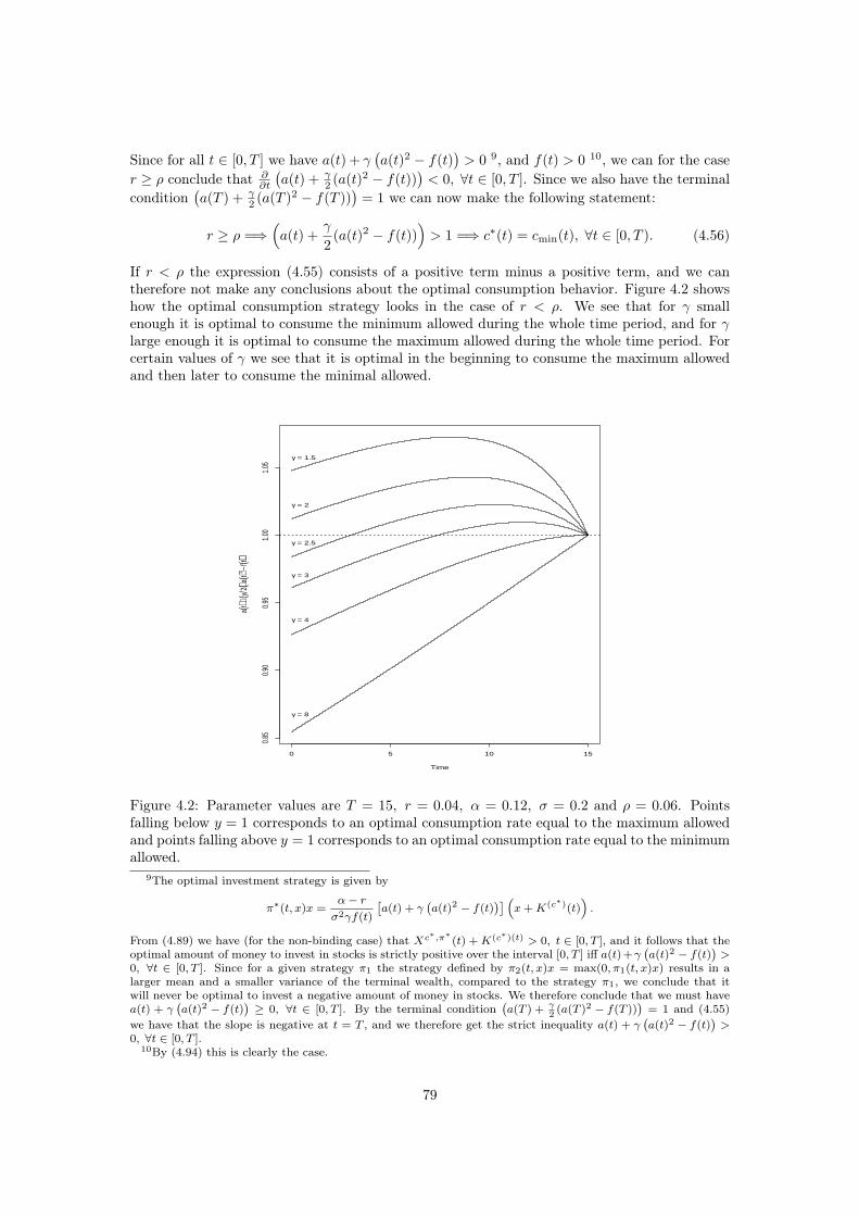
Since for all t ∈ [0, T ] we have a(t) + γ(a(t)2 − f(t)

)> 0 9, and f(t) > 0 10, we can for the case

r ≥ ρ conclude that ∂∂t

(a(t) + γ

2 (a(t)2 − f(t))

)< 0, ∀t ∈ [0, T ]. Since we also have the terminal

condition(a(T ) + γ

2 (a(T )2 − f(T ))

)= 1 we can now make the following statement:

r ≥ ρ =⇒(a(t) +

γ

2(a(t)2 − f(t))

)> 1 =⇒ c∗(t) = cmin(t), ∀t ∈ [0, T ). (4.56)

If r < ρ the expression (4.55) consists of a positive term minus a positive term, and we cantherefore not make any conclusions about the optimal consumption behavior. Figure 4.2 showshow the optimal consumption strategy looks in the case of r < ρ. We see that for γ smallenough it is optimal to consume the minimum allowed during the whole time period, and for γlarge enough it is optimal to consume the maximum allowed during the whole time period. Forcertain values of γ we see that it is optimal in the beginning to consume the maximum allowedand then later to consume the minimal allowed.

0 5 10 15

0.85

0.90

0.95

1.00

1.05

Time

a(t)+

(γ2)(

a(t)2

−f(t))

γ = 1.5

γ = 2

γ = 2.5

γ = 3

γ = 4

γ = 8

Figure 4.2: Parameter values are T = 15, r = 0.04, α = 0.12, σ = 0.2 and ρ = 0.06. Pointsfalling below y = 1 corresponds to an optimal consumption rate equal to the maximum allowedand points falling above y = 1 corresponds to an optimal consumption rate equal to the minimumallowed.

9The optimal investment strategy is given by

π∗(t, x)x =α− r

σ2γf(t)

[a(t) + γ

(a(t)2 − f(t)

)] (x+K(c∗)(t)

).

From (4.89) we have (for the non-binding case) that Xc∗,π∗(t) +K(c∗)(t) > 0, t ∈ [0, T ], and it follows that the

optimal amount of money to invest in stocks is strictly positive over the interval [0, T ] iff a(t)+γ(a(t)2 − f(t)

)>

0, ∀t ∈ [0, T ]. Since for a given strategy π1 the strategy defined by π2(t, x)x = max(0, π1(t, x)x) results in alarger mean and a smaller variance of the terminal wealth, compared to the strategy π1, we conclude that itwill never be optimal to invest a negative amount of money in stocks. We therefore conclude that we must havea(t) + γ

(a(t)2 − f(t)

)≥ 0, ∀t ∈ [0, T ]. By the terminal condition

(a(T ) + γ

2(a(T )2 − f(T ))

)= 1 and (4.55)

we have that the slope is negative at t = T , and we therefore get the strict inequality a(t) + γ(a(t)2 − f(t)

)>

0, ∀t ∈ [0, T ].10By (4.94) this is clearly the case.

79

In order to get a better understanding of the optimal consumption strategy we make thefollowing observation. If we take the optimal investment strategy as given we can try to commenton the result given by (4.56) and Figure 4.2. First of all, in contrast to the case with constantrisk aversion, the deterministic consumption strategy does influence the variance term. If we,during an infinitesimal time interval [t, t+ dt], choose to consume the minimum allowed we savethe amount of money (cmax−cmin)dt in addition to (ℓ− cmax) dt. The fraction π∗ of these moneyis invested in stocks (which do contribute to the variance term) and the rest is invested in thebank account (which do not contribute to the variance term).

For the case r ≥ ρ the expected investment return on the saved amount of money is largerthan ρ, and the mean term in (4.37) can therefore, in terms of consumption, be maximized bychoosing the minimum consumption rate allowed. We also have that a minimum consumptionrate minimizes the variance weight term γ/2(x +K(c)(t)), since a minimum consumption ratemaximizes K(c). On the other hand, choosing to consume the minimum allowed also maximizesthe variance term in (4.37) through the investment. From (4.56) we can conclude that maximizingthe mean term and minimizing the variance weight term (in terms of consumption) makes it morethan up for a larger variance term (in terms of consumption through the investment strategy).

The chain of reasoning seems to stay true for the case r < ρ. In this case the expected returnon the saved money is larger than ρ if and only if π∗ is big enough. From Figure 4.1 we havethat this is the case for a small enough value of γ. Correspondingly, Figure 4.2 shows that itis optimal to consume the minimum (maximum) allowed for a small (large) enough value of γ.The reason that it is optimal for an investor with a given value of γ (not too large neither toosmall) first to consume the maximum allowed and after some time the minimum allowed is dueto the fact that π∗ is increasing in time.

4.5 Mean-standard deviation without pre-commitmentIn this section we study and solve the mean-standard deviation problem without pre-commitmentincluding consumption and terminal wealth. We consider a general risk aversion function ψ,which we assume fulfills some reasonable constraints, and show that the optimal investmentstrategy becomes the same (π∗ = 0) for all variants of ψ. Finally, we give an interpretation ofthe optimal strategy which also helps us understand the fundamental difference between pre-commitment and without pre-commitment.

4.5.1 Presenting and solving the problemConsider the problem of finding the optimal strategy for the objective given by

E0,x0

[∫ T

0

e−ρsc(s)ds+ e−ρTXc,π(T )

]− ψ(0, x0)

(V ar0,x0

[∫ T

0

e−ρsc(s)ds+ e−ρTXc,π(T )

]) 12

,

(4.57)

where ψ ∈ C1,2, ψ > 0, is a risk aversion function with ψx, ψxx and ψt finite ∀(t, x) ∈ [0, T ]×R,and where we again restrict the admissible strategies to (c, π) ∈ A

∩(D × R), where D(s) =

[cmin(s), cmax(s)], s ∈ [0, T ], is a finite time dependent interval. The corresponding function fis given by

f(t, x, y, z) = y − ψ(t, x)(z − y2

) 12 .

80

The system of partial differential equations we want to solve in order to obtain the optimal valuefunction and the optimal strategy is given by (4.16) and (4.17)11. Clearly,

ft = −ψt

(z − y2

) 12 , fx = −ψx

(z − y2

) 12 , fxx = −ψxx

(z − y2

) 12 ,

fy = 1 + ψ(z − y2

)−12 y, fyy = ψ

(z − y2

)−32 y2 + ψ

(z − y2

)−12 ,

fz = −ψ2

(z − y2

)−12 , fzz =

ψ

4

(z − y2

)−32 ,

fxz = −ψx

2

(z − y2

)−12 , fxy = ψx

(z − y2

)−12 y, fyz =

−ψ2

(z − y2

)−32 y.

Inserting this in (4.19)–(4.21) we obtain the following expression

Q = −ψx

(F (2) −

(F (1)

)2) 12

, (4.58)

U =ψ

4

(F (2) −

(F (1)

)2)− 32 (F (2)x − 2F (1)F (1)

x

)2+ ψ

(F (2) −

(F (1)

)2)− 12 (F (1)x

)2− ψxx

(F (2) −

(F (1)

)2) 12

− ψx

(F (2) −

(F (1)

)2)− 12 (F (2)x − 2F (1)F (1)

x

), (4.59)

J = ρF (1) − c− ψρ

(F (2) −

(F (1)

)2) 12

− ψt

(F (2) −

(F (1)

)2) 12

. (4.60)

We are now ready to derive a candidate for the optimal strategy. Again this is done by differen-tiating with respect to c and π inside the curly brackets in (4.16). We get

c∗(t, x) =

cmax(t), if C(t, x) < 0,

non-defined, if C(t, x) = 0,

cmin(t), if C(t, x) > 0,

(4.61)

where

C(t, x) := Fx(x, t)−Q(x, t)− 1−(∂

∂cψt

)(F (2) −

(F (1)

)2) 12

,

and

π∗(t, x)x = −α− r

σ2

Fx −Q

Fxx − U, (4.62)

(provided U > Fxx). We now search for solutions in the form,

F (t, x) = A(t)x+B(t),

F (1)(t, x) = a(t)x+ b(t),

where A, B, a, and b are deterministic functions of time. The derivatives of interest are

Ft = A′(t)x+B′(t), Fx = A(t), Fxx = 0,

F(1)t = a′(t)x+ b′(t), F (1)

x = a(t), F (1)xx = 0.

11Since Ft = F(1)t − ∂

∂tψ(t, x)

(F (2) −

(F (1)

)2) 12 − ψ(t,x)

2

(F (2) −

(F (1)

)2)− 12(F

(2)t − 2F (1)F

(1)t

)we only

need to solve two of the three differential equations given by (4.16)–(4.18). We choose to solve (4.16) and (4.17).

81

Inserting this into the system of partial differential equations given by (4.16) and (4.17) we find

Atx+Bt = −rx(A−Q)− 1

2π∗(α− r)x(A−Q)− ℓ(A−Q) + c∗(A−Q) + J,

atx+ bt = −rxa− π∗(α− r)xa− ℓa+ c∗(a− 1) + ρ(ax+ b).

Quite surprisingly, this system of differential equations is solved by π∗ = 0 via the parametriza-tion F (2) =

(F (1)

)2 12. Note that for this solution, actually U is infinite. However since π∗Uis finite, the solution is admissible. With π∗ = 0 the system of partial differential equationsreduces to

Atx+Bt = −rxA+ ρxa− ℓA+ c∗(A− 1) + ρb,

A(T ) = 1,

B(T ) = 0,

atx+ bt = −(r − ρ)xa− ℓa+ c∗(a− 1) + ρb,

a(T ) = 1,

b(T ) = 0,

where we have added the terminal conditions. We obtain the solutions

A(t) = a(t) = e(r−ρ)(T−t),

and

B(t) = b(t) = eρt∫ T

t

[ℓ(s)e(r−ρ)(T−s) − c∗(s)

(e(r−ρ)(T−s) − 1

)]e−ρsds.

The optimal strategy now follows directly by plugging in the solutions for A and a together withthe partial derivatives and the relation F (2) =

(F (1)

)2into (4.61) and (4.62). We summarize

the results as follows.

12F (2) =(F (1)

)2 implies that F (2)x − 2F (1)F

(1)x = 0. Inserting this into (4.58) and (4.59) gives

Q = 0,

U = ψ(t, x)

(F (2) −

(F (1)

)2)− 1

2 (F

(1)x

)2.

Formula (4.62) now reduces to

π∗(t, x)x = −α− r

σ2

A(t)(F (2) −

(F (1)

)2) 12

ψ(t, x)(F

(1)x

)2.

It is then clear that(F (2) =

(F (1)

)2)

⇒ (π∗ = 0)

⇔

F

(1)x = 0 and A(t) bounded from above

.

Below we show that F (1)x = a(t) = A(t) = er(T−t) > 0, and clearly we get π∗ = 0.

82

Proposition 4.5.1. For the mean-standard deviation problem given by (4.57) we have the fol-lowing results.

• The optimal strategy is given by

c∗(t, x) =

cmax(t), if r < ρ,

non-defined, if r = ρ,

cmin(t), if r > ρ,

π∗(t, x) = 0.

• The optimal value function is given by

V (t, x) = e(r−ρ)(T−t)x+B(t).

• The conditional expected value of the discounted cumulated optimal consumption plus thediscounted optimal terminal wealth is given by

Et,x

[∫ T

t

e−ρ(s−t)c∗(s)ds+ e−ρ(T−t)Xc∗,π∗(T )

]= e(r−ρ)(T−t)x+ b(t).

• The conditional variance of the discounted cumulated optimal consumption plus the dis-counted optimal terminal wealth is given by

V art,x

[∫ T

t

e−ρ(s−t)c∗(s)ds+ e−ρ(T−t)Xc∗,π∗(T )

]= 0.

Here

B(t) = b(t) = eρt∫ T

t

[ℓ(s)e(r−ρ)(T−s) − c∗(s)

(e(r−ρ)(T−s) − 1

)]e−ρsds.

4.5.2 Discussion of the solutionThe optimal consumption strategy coincides with the one found in Chapter 4.3. We refer toSubsection 4.3.2 for an interpretation.

The following intuitive explanation of the somehow surprising optimal investment strategy(π∗ = 0) actually provides us with some helpful insight to understand the nature of inconsistentstochastic optimization problems. In discrete time, the definition of a subgame Nash equilibriumstrategy is: Consider n players and split the time interval [T0, Tn] in n equally long intervals. Letplayer m, 1 ≤ m ≤ n, decide on the strategy (c∗m−1, π

∗m−1) used over the interval [Tm−1, Tm).

• The equilibrium control (c∗n−1, π∗n−1) is obtained by letting player n optimize the value

function at time Tn−1.

• The equilibrium control (c∗n−2, π∗n−2) is obtained by letting player n− 1 optimize the value

function at time Tn−2 given the knowledge that player number n will use the strategy(c∗n−1, π

∗n−1).

• Proceed recursively by induction.

Now, consider a single period pure portfolio optimization problem with time horizon ∆t givenby

V (0, x) = supπ

E0,x [X

π(∆t)]− ψ(0, x) (V ar0,x [Xπ(∆t)])

12

,

83

where Xc,π(∆t) = r∆t(1 − π)x + Rπx and R is a random variable such that E[R] = α∆t andV ar[R] = σ2∆t. Then we have

E0,x [Xπ(∆t)]− ψ(0, x) (V ar0,x [X

π(∆t)])12

= r∆tx+ (α− r)πx∆t− ψ(0, x)(σ2∆tπ2x2

) 12

= r∆tx+ (α− r)πx∆t− ψ(0, x)σ√∆t|π|x.

We directly obtain the optimal strategy

π∗ =

0, if (α− r)∆t < ψ(0, x)σ

√∆t,

non-defined(R+), if (α− r)∆t = ψ(0, x)σ√∆t,

∞, if (α− r)∆t > ψ(0, x)σ√∆t.

Clearly, for any risk aversion function ψ(0, x) there exist a small enough ∆t such that (α−r)∆t <ψ(0, x)σ

√∆t, i.e. such that π∗ = 0 13. Likewise, for a multi period problem we conclude that

for any risk aversion function ψ(t, x), fulfilling our reasonable assumptions, we get the Nashequilibrium strategy π∗ = 0 whenever the discretization of the interval of optimization is fineenough. To obtain this note, by the argumentation above, that for a fine enough discretizationof the interval player n (the last player in the game) chooses to take no risk at all. Consequently,player number n − 1 faces, since there is no randomness after time Tn−1, also a single periodproblem and by the same argumentation player number n− 1 also chooses to take no risk at all.Proceeding recursively we obtain π∗ = 0 for all players.

For any risk aversion function ψ(t, x), fulfilling our reasonable assumptions, we now concludethat over an infinitesimal time interval, dt, standard deviation is of the order

√dt, which means

that the punishment is so hard that any risk taking is unattractive.

AcknowledgmentsThe authors wish to thank the anonymous referee for an extremely detailed and valuable corre-spondence and Esben Masotti Kryger for valuable discussions and comments.

4.6 Appendix

4.6.1Proof of Theorem 4.2.1. Consider an arbitrary admissible strategy (c, π).

1: First we argue that if there exist a function Y such that, ∀(t, x) ∈ (0, T )× R, we have

Yt = −[(r + π(α− r))x+ ℓ− c]Yx − 1

2π2σ2x2Yxx − c+ ρY, (4.63)

Y (T, x) = x, (4.64)

then

Y (t, x) = yc,π(t, x), (4.65)

where yc,π is given by (4.14).

13This is also indicated by Zhou and Li (2000) who get the same solution for a sufficiently short time horizon.

84

To show this define

Y (t, x) = e−ρtY (t, x). (4.66)

From (4.63) and (4.64) we get, ∀(t, x) ∈ (0, T )× R, that

Yt = −[(r + π(α− r))x+ ℓ− c]Yx − 1

2π2σ2x2Yxx − e−ρtc, (4.67)

Y (T, x) = e−ρTx. (4.68)

Using Itô’s formula

Y (t,Xc,π(t))

= −∫ T

t

dY (s,Xc,π(s)) + Y (T,Xc,π(T ))

= −∫ T

t

(Ys(s,X

c,π(s)) + [(r + π(s)(α− r))Xc,π(s) + ℓ(s)− c(s)] Yx(s,Xc,π(s))

+1

2π(s)2σ2Xc,π(s)2Yxx(s,X

c,π(s)))ds

−∫ T

t

π(s)σXc,π(s)Yx(s,Xc,π(s))dW (s) + Y (T,Xc,π(T )).

Plug in (4.67) and (4.68) to obtain

Y (t,Xc,π(t)) =

∫ T

t

e−ρsc(s)ds+ e−ρTXc,π(T )−∫ T

t

π(s)σXc,π(s)Yx(s,Xc,π(s))dW (s).

(4.69)

Since (c, π) is an admissible strategy taking the conditional expectation given X(t) = x on bothsides of the equality leaves us with

Y (t, x) = E

[∫ T

t

e−ρsc(s)ds+ e−ρTXc,π(T )

∣∣∣∣∣ X(t) = x

].

It is now clear that

Y (t, x) = eρtY (t, x) = yc,π(t, x).

2: Second we argue that if there exist a function Z such that, ∀(t, x) ∈ (0, T )× R, we have

Zt = −[(r + π(α− r))x+ ℓ− c]Zx − 1

2π2σ2x2Zxx − 2cY + 2ρZ, (4.70)

Z(T, x) = x2, (4.71)

then

Z(t, x) = zc,π(t, x), (4.72)

where zc,π is given by (4.15).

To show this define Z(t, x) = e−2ρtZ(t, x). From (4.70) and (4.71) we get, ∀(t, x) ∈ (0, T )×R,that

Zt = −[(r + π(α− r))x+ ℓ− c]Zx − 1

2π2σ2x2Zxx − 2e−ρtcY , (4.73)

Z(T, x) =(e−ρTx

)2, (4.74)

85

where Y (t, x) is given in (4.66). Using Itô’s formula

Z(t,Xc,π(t))

= −∫ T

t

dZ(s,Xc,π(s)) + Z(T,Xc,π(T ))

= −∫ T

t

(Zs(s,X

c,π(s)) + [(r + π(s)(α− r))Xc,π(s) + ℓ(s)− c(s)] Zx(s,Xc,π(s))

+1

2π(s)2σ2Xc,π(s)2Zxx(s,X

c,π(s)))ds

−∫ T

t

π(s)σXc,π(s)Zx(s,Xc,π(s))dW (s) + Z(T,Xc,π(T )).

Plug in (4.73) and (4.74) and thereafter (4.69) to obtain

Z(t,Xc,π(t))

= 2

∫ T

t

e−ρsc(s)Y (s,Xc,π(s))ds+(e−ρTXc,π(T )

)2(4.75)

−∫ T

t

π(s)σXc,π(s)Zx(s,Xc,π(s))dW (s)

= 2

∫ T

t

e−ρsc(s)

∫ T

s

e−ρyc(y)dyds+ 2

∫ T

t

e−ρsc(s)ds e−ρTXc,π(T )

− 2

∫ T

t

e−ρsc(s)

∫ T

s

π(y)σXc,π(y)Yx(y,Xc,π(y))dW (y)ds

+(e−ρTXc,π(T )

)2 − ∫ T

t

π(s)σXc,π(s)Zx(s,Xc,π(s))dW (s). (4.76)

Since (c, π) is an admissible strategy taking the conditional expectation given X(t) = x on bothsides of the equality leaves us with

Z(t, x) = E

[2

∫ T

t

e−ρsc(s)

∫ T

s

e−ρyc(y)dyds

+ 2

∫ T

t

e−ρsc(s)ds e−ρTXc,π(T ) +(e−ρTXc,π(T )

)2 ∣∣∣∣∣ X(t) = x

].

Provided that 2∫ T

te−ρsc(s)

∫ T

se−ρyc(y)dyds =

(∫ T

te−ρsc(s)ds

)2we now have that

Z(t, x) = E

(∫ T

t

e−ρsc(s)ds+ e−ρTXc,π(T )

)2 ∣∣∣∣∣ X(t) = x

.This is however easily realized since

∂

∂t

(2

∫ T

t

e−ρsc(s)

∫ T

s

e−ρyc(y)dyds

)= −2e−ρtc(t)

∫ T

t

e−ρyc(y)dy =∂

∂t

(∫ T

t

e−ρsc(s)ds

)2

(2

∫ T

t

e−ρsc(s)

∫ T

s

e−ρyc(y)dyds

)∣∣t=T

= 0 =

(∫ T

t

e−ρsc(s)ds

)2

∣∣t=T

.

86

It is now clear that

Z(t, x) = e2ρtZ(t, x) = zc,π(t, x).

3: At last we argue that if there exist a function F such that, ∀(t, x) ∈ (0, T )× R, we have

Ft = inf(c,π)∈A

−[(r + π(α− r))x+ ℓ− c](Fx − fx)−

1

2π2σ2x2(Fxx − U) + J

, (4.77)

F (T, x) = f(T, x, x, x2

), (4.78)

where

U = fxx +(F (1)x

)2fyy +

(F (2)x

)2fzz + 2F (1)

x F (2)x fyz + 2F (1)

x fxy + 2F (2)x fxz, (4.79)

J =(ρF (1) − c

)fy + 2

(ρF (2) − cF (1)

)fz + ft, (4.80)

with F (1) and F (2) fulfilling (4.17) and (4.18), respectively, then

F (t, x) = V (t, x),

where V is the optimal value function defined by (4.11).

First step is to derive an expression for

f(t,Xc,π(t), yc,π(t,Xc,π(t)), zc,π(t,Xc,π(t))).

By (4.65) and (4.72) this equals

f(t,Xc,π(t), Y (t,Xc,π(t)), Z(t,Xc,π(t))).

Using Itô’s formula(we have assumed f ∈ C1,2,2,2

)we get that

f(t,Xc,π(t), yc,π(t,Xc,π(t)), zc,π(t,Xc,π(t)))

= −∫ T

t

df(s,Xc,π(s), Y (s,Xc,π(s)), Z(s,Xc,π(s)))

+f(T,Xc,π(T ), Y (T,Xc,π(T )), Z(T,Xc,π(T )))

= −∫ T

t

(fs + fyYs + fzZs)ds+ (fx + fyYx + fzZx)dX

c,π(s)

+1

2

[fyYxx + fzZxx + fxx + fyy (Yx)

2+ fzz (Zx)

2

+2fxyYx + 2fxzZx + 2fyzYxZx

]π(s)2σ2Xc,π(s)2ds

+f(T,Xc,π(T ), Y (T,Xc,π(T )), Z(T,Xc,π(T ))), (4.81)

where we have skipped some arguments under the integral. Inserting (4.63), (4.70) and the

87

dynamics of X given by (4.5) we have that

f(t,Xc,π(t), yc,π(t,Xc,π(t)), zc,π(t,Xc,π(t)))

= −∫ T

t

[fs + fy

(−[(r + π(s)(α− r))Xc,π(s) + ℓ(s)− c(s)

]Yx

−1

2π(s)2σ2Xc,π(s)2Yxx − c(s) + ρY

)+fz

(−[(r + π(s)(α− r))Xc,π(s) + ℓ(s)− c(s)

]Zx

−1

2π(s)2σ2Xc,π(s)2Zxx − 2c(s)Y + 2ρZ

)]ds

+(fx + fyYx + fzZx)([

(r + π(s)(α− r))Xc,π(s) + ℓ(s)− c(s)]ds+ π(s)σXc,π(s)dW (s)

)+1

2

[fyYxx + fzZxx + fxx + fyy (Yx)

2+ fzz (Zx)

2

+2fxyYx + 2fxzZx + 2fyzYxZx

]π(s)2σ2Xc,π(s)2ds

+f(T,Xc,π(T ), Y (T,Xc,π(T )), Z(T,Xc,π(T ))).

After reduction this is

f(t,Xc,π(t), yc,π(t,Xc,π(t)), zc,π(t,Xc,π(t)))

= −∫ T

t

(fs + fy

(− c(s) + ρY

)+ fz

(− 2c(s)Y + 2ρZ

))ds

+fx[(r + π(s)(α− r))Xc,π(s) + ℓ(s)− c(s)

]ds+ (fx + fyYx + fzZx)π(s)σX

c,π(s)dW (s)

+1

2

[fxx + fyy (Yx)

2+ fzz (Zx)

2+ 2fxyYx + 2fxzZx + 2fyzYxZx

]π(s)2σ2Xc,π(s)2ds

+f(T,Xc,π(T ), Y (T,Xc,π(T )), Z(T,Xc,π(T ))).

Define for an arbitrary admissible strategy (c, π) the quantities corresponding to (4.79) and(4.80) by

U = fxx + (Yx)2fyy + (Zx)

2fzz + 2YxZxfyz + 2Yxfxy + 2Zxfxz, (4.82)

J = (ρY − c) fy + 2 (ρZ − cY ) fz + ft. (4.83)

We now get

f(t,Xc,π(t), yc,π(t,Xc,π(t)), zc,π(t,Xc,π(t)))

= −∫ T

t

J(s) + fx

[(r + π(s)(α− r))Xc,π(s) + ℓ(s)− c(s)

]ds

+(fx + fyYx + fzZx)π(s)σXc,π(s)dW (s) +

1

2U(s)π(s)2σ2Xc,π(s)2ds

+f(T,Xc,π(T ), Y (T,Xc,π(T )), Z(T,Xc,π(T ))). (4.84)

Next step is, by use of (4.84), to show that for any admissible strategy (c, π) we have

f(t, x, yc,π(t, x), zc,π(t, x))

≤ F (t, x) +

∫ T

t

(J(s)− J(s) +

1

2σ2π(s)2Xc,π(s)2(U(s)− U(s))

)ds. (4.85)

88

By use of Itô’s formula we get that

F (t,Xc,π(t)) = −∫ T

t

dF (s,Xc,π(s)) + F (T,Xc,π(T ))

= −∫ T

t

(Fsds+ FxdX

c,π(s) +1

2Fxxπ(s)

2σ2Xc,π(s)2ds

)+ F (T,Xc,π(T )).

Since F solves the pseudo Hamilton-Jacobi-Bellman equation (4.77) we see that for the arbitrarystrategy (c, π) we have, ∀(t, x) ∈ (0, T )× R, that

Ft ≤ −[(r + π(α− r))x+ ℓ− c

](Fx − fx)−

1

2π2σ2x2(Fxx − U) + J.

Inserting this with x = Xc,π(s), inserting the dynamics of X given by (4.5), and inserting theterminal conditions (4.78), (4.64) and (4.71) we get that

F (t,Xc,π(t)) ≥ −∫ T

t

(−[(r + π(α− r))Xc,π(s) + ℓ(s)− c(s)

](Fx − fx)

− 1

2π(s)2σ2Xc,π(s)2(Fxx − U(s)) + J(s)

)ds

+ Fx

([(r + π(s)(α− r))Xc,π(s) + ℓ(s)− c(s)

]ds+ π(s)σXc,π(s)dW (s)

)+

1

2Fxxπ(s)

2σ2Xc,π(s)2ds

+ f(T,Xc,π(T ), Y (T,Xc,π(T )), Z(T,Xc,π(T ))).

After reduction this is

F (t,Xc,π(t)) ≥ −∫ T

t

(fx[(r + π(α− r))Xc,π(s) + ℓ(s)− c(s)

]+

1

2π(s)2σ2Xc,π(s)2U(s) + J(s)

)ds+ Fxπ(s)σX

c,π(s)dW (s)

+ f(T,Xc,π(T ), Y (T,Xc,π(T )), Z(T,Xc,π(T ))).

Insert (4.84) to obtain

F (t,Xc,π(t)) ≥∫ T

t

(fx + fyYx + fzZx − Fx

)π(s)σXc,π(s)dW (s)

−∫ T

t

(J(s)− J(s) +

1

2σ2π(s)2Xc,π(s)2(U(s)− U(s))

)ds

+ f(t,Xc,π(t), yc,π(t,Xc,π(t)), zc,π(t,Xc,π(t))). (4.86)

Since (c, π) is an arbitrarily chosen admissible strategy, taking the conditional expectation givenX(t) = x of the inequality gives (4.85).

Consider now the specific strategy (c∗, π∗) fulfilling the infimum in (4.77). By (4.65) and(4.72) it follows that

F (1)(t, x) = yc∗,π∗

(t, x),

F (2)(t, x) = zc∗,π∗

(t, x).

89

Final step is to show that the Nash equilibrium criteria given by Definition 4.2.1 is fulfilled.

Going through the same calculations as above, and using that for the specific strategy (c∗, π∗)we have, ∀(t, x) ∈ (0, T )× R, that

Ft = −[(r + π∗(α− r))x+ ℓ− c∗](Fx − fx)−1

2(π∗)2σ2x2 (Fxx − U) + J,

we get

F(t,Xc∗,π∗

(t))=

∫ T

t

(fx + fyYx + fzZx − Fx)π

∗(s)σXc∗,π∗(s)dW (s)

+ f

(t,Xc∗,π∗

(t), Y(t,Xc∗,π∗

(t)), Z(t,Xc∗,π∗

(t)))

. (4.87)

Since (c∗, π∗) is an admissible strategy, taking the conditional expectation given X(t) = x onboth sides of the inequality we obtain

F (t, x) = f(t, x, yc

∗,π∗(t, x), yc

∗,π∗(t, x)

). (4.88)

Now let (ch, πh) be defined by (4.10). To make it explicit that the expressions in (4.82) and(4.83) depend on h, when using the strategy (ch, πh), we write Uh and Jh, respectively. By (4.85)and (4.88) we get that

limh→0

inff(t, x, yc

∗,π∗(t, x), zc

∗,π∗(t, x)

)− f

(t, x, ych,πh(t, x), zch,πh(t, x)

)h

= limh→0

inf

∫ T

t

(Jh(s)− J(s) + 1

2σ2πh(s)

2X ch,πh(s)2(Uh(s)− U(s)))ds

h

= limh→0

inf

∫ t+h

t

(Jh(s)− J(s) + 1

2σ2π(s)2Xc,π(s)2(Uh(s)− U(s))

)ds

h

= J0(t)− J(t) +1

2σ2π(t)2Xc,π(t)2(U0(t)− U(t))

= 0,

where we have used that (ch, πh) coincides with (c∗, π∗) on [t+h, T ], and with (c, π) on [t,t+h).We conclude that F (t, x) = V (t, x), and that (c∗, π∗) is the corresponding optimal strategy.

90

4.6.2First. We want to show that the assumption made in (4.44) given as

a(t)b(t) =g(t)

2

is fulfilled. This is easily seen to be the case since a(T )b(T ) = g(T )2 = 0, and by use of (4.52)

and (4.53)

∂

∂t(a(t)b(t)) = a′(t)b+ ab′(t)

= −(r − ρ) +

(α− r)2

σ2γf(t)

[a(t) + γ(a(t)2 − f(t))

]a(t)b(t)− c∗(t)a(t) + ρa(t)b(t),

and

g′(t)

2= −

(r − ρ) +

(α− r)2

σ2γf(t)

[a(t) + γ(a(t)2 − f(t))

] g(t)

2− c∗(t)a(t) + ρ

g(t)

2.

Second. We want to show that the condition (4.51) for the non-binding case given as

γf(t)

x+K(c∗)(t)> 0, ∀(t, x) ∈ [0, T )× R,

required for the investment strategy (4.50) to be optimal, is fulfilled.

In order to verify this condition notice that by use of the candidate for the optimal strategygiven by (4.49) and (4.50) we get that

d(Xc∗,π∗

(t) +K(c∗)(t))

=

[rXc∗,π∗

(t) +(α− r)2

σ2γf(t)

[a(t) + γ

(a(t)2 − f(t)

)] (Xc∗,π∗

(t) +K(c∗)(t))+ ℓ(t)− c∗(t)

]dt

+α− r

σγf(t)

[a(t) + γ

(a(t)2 − f(t)

)] (Xc∗,π∗

(t) +K(c∗)(t))dW (t) +

(rK(c∗)(t)− ℓ(t) + c∗(t)

)dt

=

(r +

(α− r)2

σ2γf(t)

[a(t) + γ

(a(t)2 − f(t)

)])(Xc∗,π∗

(t) +K(c∗)(t))dt

+α− r

σγf(t)

[a(t) + γ

(a(t)2 − f(t)

)] (Xc∗,π∗

(t) +K(c∗)(t))dW (t).

We see that (Xc∗,π∗(t) +K(c∗)(t)) takes the form of a geometric Brownian motion. We get the

solution

Xc∗,π∗(t) +K(c∗)(t)

=(x0 +K(c∗)(0, x0)

)exp

∫ t

0

(r +

(α− r)2

σ2γf(s)

[a(s) + γ

(a(s)2 − f(s)

)]− 1

2

(α− r)2

σ2γ2f(s)2[a(s) + γ

(a(s)2 − f(s)

)]2)ds+

∫ t

0

α− r

σγf(s)

[a(s) + γ

(a(s)2 − f(s)

)]dW (s)

.

(4.89)

From (4.94) below it follows that f is a strictly positive function over the time interval [0, T ).Finally, since for the non-binding case x0 +K(c∗)(0, x0) > 0 we conclude that the condition isfulfilled.

91

Third. We want to show that the highly non-linear system of partial differential equations givenby (4.52) and (4.53) has a unique global solution. In order to show this take conditional expec-tation in (4.89) for t = T to get that (remember that K(c∗)(T ) = 0)

Et,x

[Xc∗,π∗

(T )]=(x+K(c∗)(t)

)e∫ Tt

[r+(α−r)π∗(s)]ds (4.90)

Et,x

[(Xc∗,π∗

(T ))2]

=(x+K(c∗)(t)

)2e2

∫ Tt [r+(α−r)π∗(s)+ 1

2σ2π∗(s)2]ds, (4.91)

where14

π∗(t) =α− r

σ2γf(t)

[a(t) + γ

(a(t)2 − f(t)

)]. (4.92)

We now get that

a(t)(x+K(c∗)(t)

)+ b(t)

= Et,x

[∫ T

t

e−ρ(s−t)c∗(s)ds+ e−ρ(T−t)Xc∗,π∗(T )

]

=(x+K(c∗)(t)

)e∫ Tt

[(r−ρ)+(α−r)π∗(s)]ds +

∫ T

t

e−ρ(s−t)c∗(s)ds

and

f(t)(x+K(c∗)(t)

)2+ g(t)

(x+K(c∗)(t)

)+ h(t)

= Et,x

(∫ T

t

e−ρ(s−t)c∗(s)ds+ e−ρ(T−t)Xc∗,π∗(T )

)2

= e−2ρ(T−t)Et,x

[(Xc∗,π∗

(T ))2]

+ 2

(∫ T

t

e−ρ(s−t)c∗(s)ds

)e−ρ(T−t)Et,x

[Xc∗,π∗

(T )]

+

(∫ T

t

e−ρ(s−t)c∗(s)ds

)2

=(x+K(c∗)(t)

)2e2

∫ Tt [(r−ρ)+(α−r)π∗(s)+ 1

2σ2π∗(s)2]ds

+2

(∫ T

t

e−ρ(s−t)c∗(s)ds

)(x+K(c∗)(t)

)e∫ Tt

[(r−ρ)+(α−r)π∗(s)]ds

+

(∫ T

t

e−ρ(s−t)c∗(s)ds

)2

.

14Notice that π defines the optimal proposition of Xc∗,π∗+K(c∗) to invest in stocks S.

92

Collecting terms we obtain

a(t) = e∫ Tt

[(r−ρ)+(α−r)π∗(s)]ds, (4.93)

b(t) =

∫ T

t

e−ρ(s−t)c∗(s)ds,

f(t) = e2∫ Tt [(r−ρ)+(α−r)π∗(s)+ 1

2σ2π∗(s)2]ds, (4.94)

g(t) = 2e∫ Tt

[(r−ρ)+(α−r)π∗(s)]ds

∫ T

t

e−ρ(s−t)c∗(s)ds,

h(t) =

(∫ T

t

e−ρ(s−t)c∗(s)ds

)2

.

Now insert (4.93) and (4.94) into (4.92) to get the following integral equation for π∗

π∗(t) =α− r

σ2γf(t)

[a(t) + γ

(a(t)2 − f(t)

)]=α− r

σ2γ

e−

∫ Tt [(r−ρ)+(α−r)π∗(s)+σ2π∗(s)2]ds + γe−

∫ Tt

σ2π∗(s)2ds − γ. (4.95)

The key question now is whether the integral equation (4.95) has a unique global solution.Fortunately this is the case. The technical work is done in Björk et al. (2012). They show thatthe algorithm given by

π0(t) := 1,

πn+1(t) =α− r

σ2γ

[e−

∫ Tt

[(r−ρ)+(α−r)πn(s)+σ2π2n(s)]ds + γe−

∫ Tt

σ2π2n(s)ds − γ

], (4.96)

converges in C[0, T ], and that the full sequence πn converges to the solution π∗.

93

94

5. Why you should care about investmentcosts: A risk-adjusted utility approach

Abstract: Under the assumption of zero correlation between cost ratios and ex-pected investment returns we analyze the impact of proportional investment costs. Weconsider a constant relative risk aversion investor optimizing expected utility from ter-minal wealth and identify, in addition to the direct effect due to the additional costsincurred, an indirect effect due to a less risky stock position induced by investmentcosts. By use of an indifferent compensation measure, defined as the minimum relativeincrease in the initial wealth the investor demands in compensation to accept incurringinvestment costs of a certain size, we quantify the impact of investment costs. We ob-tain, for realistic parameters for risk aversion and the financial market, the surprisingresults that the indirect effect is between half (myopic investor) and the same (longterm investor) size as the direct effect, and that the investment decision seems to beof very little importance compared to the size of the investment costs.

Keywords: Investment costs, risk aversion, stochastic control, indifferent compen-sation measure, certainty equivalents.

5.1 IntroductionMost investors seem primarily to focus on the ability of excellent stock picking, when decidingwhich fund should manage their savings. At the same time costs charged by funds seem to differby a great deal. The average U.S. equity mutual fund charges around 1.3–1.5 percent, but costratios range from as low as 0.2 (index funds) to as high as 2 percent. In general, costs can varysubstantially across comparable funds, and larger funds and fund complexes charge lower costs(see e.g. Khorana et al. (2008)). Clearly, the argument for charging high costs is excellent stockpicking. The expensive fund managers are likely to claim that the additional return they areexpected to generate (compared to any cheaper fund manager) more than compensates for theextra costs. However, the vast majority of the large literature analyzing whether excellent stockpicking skills exist rejects this hypothesis. This is e.g. demonstrated by Gil-Bazo and Ruiz-Verdú(2009) who consider a data set including all open-end U.S. mutual funds that are active in the1961 to 2005 period. They consider a series of robustness checks consisting of checking for theimpact of funds with extreme cost ratios and extreme risk-adjusted performance; the impactof small funds; exclusive focussing on funds for which annual operating costs account for 100percent of all costs or focussing only on funds with loads; splitting time into subperiods; split-ting mutual funds into categories. In all cases the conclusion stays the same: The hypothesisof a unit slope relation between risk-adjusted before-fee performance and cost ratios falls at anyconventional significance level. In fact, ironically, the estimated slope becomes negative. See alsoCarhart (1997) who, using the same data set, concludes that higher costs depress investmentperformance while increasing fund companies’ profitability. Also Fama and French (2010) reportthat only very few funds produce benchmark-adjusted expected returns sufficient to cover theircosts. One of the reasons that some funds are more expensive is due to the more actively man-aged investments. Huang et al. (2013) report, using a sample of 2979 U.S. equity funds over theperiod between 1980 and 2009, that the top and bottom decile of funds on average change theirannualized volatility by more than six percentage points. They also find, by use of a holding-based measure of risk shifting, that funds which alter risk perform worse than funds that keep

95

stable risk levels over time, suggesting that risk shifting either is an indication of inferior abilityor is motivated by agency issues. Summing up, it seems hard to prove that good performance isanything but a random phenomena.

Consequently, the impact of investment costs is naturally analyzed under the assumption ofa zero correlation between the cost ratio and the expected investment return. The literature, e.g.the references above, seems only to focus on the loss in rate of return. However, the loss in rateof return simply induced by paying higher investment costs might not describe the actual losssuffered by the investor. A more sophisticated approach would be to take into account the riskaversion of the investor when evaluating the impact of investment costs, thereby also introducinga change in the investment strategy induced by investment costs. Introducing proportionalinvestment costs and by use of utility functions, this is the approach taken in our paper. Tworelated papers, also taking the investor’s risk aversion into account while considering proportionalcosts are Guillén et al. (2013) and Palczewski et al. (2013) (the latter analyzes the impact oftransaction costs).

Guillén et al. (2013) consider a Value at Risk investor (VaR-investor) who invests in a Black-Scholes market concerned about a given α-percent quantile of the terminal wealth distribution.By introducing investment costs the investor is forced to invest less in the stock market in orderto maintain the same α-percent quantile. Consequently, the loss in the geometric rate of returnsplits into two effects: (a) A direct effect due to the additional expense incurred and (b) anindirect effect due to a less risky stock position. Some of the capital the investor, prior tointroducing investment costs, was willing to risk losing is now used to pay investment costs.Guillén et al. (2013) refer to the indirect effect as loss of investment opportunities. The maindrawback of the VaR-approach is that no monetary quantification of how much the investoractually suffers from investment costs seems to be possible. Focussing at the geometric rate ofreturn seems a bit ad hoc since, in the first place, when deciding upon the investment strategy,the VaR-investor had no particular preferences for a high median. Using the geometric rate ofreturn to measure the impact of investment costs also restricts the parameter space since forvery risk seeking investors, introducing investment costs actually increases the geometric rate ofreturn.

In contrast, Palczewski et al. (2013) use utility functions, but focus instead on the impactof transaction costs. They optimize expected utility from investing in a market consisting of arisk free asset and a risky asset modeled by a diffusion model with state-dependent drift. Theeffect of costs can again be divided into a direct and an indirect effect. This time the indirecteffect is due to less trading in the asset portfolio. By calculating the indifference price, definedas the amount of money the investor is willing to pay up front to avoid incurring transactioncosts, they find that in general the loss in utility due to proportional transaction costs is abouttwice as large as the direct expenses incurred.

Similar findings are offered by our paper for the case of proportional investment costs. Wefocus on a constant relative risk aversion (CRRA) utility optimizer who hands over his savingsto a fund investing in a frictionless Black-Scholes market while being charged proportional in-vestment costs. As in Guillén et al. (2013) and Palczewski et al. (2013) we obtain a direct and anindirect effect due to a change in investment costs. In contrast to the VaR-approach of Guillénet al. (2013) the change in investment strategy and, consequently, the change in geometric rate ofreturn induced by a change in investment costs becomes independent of the investment horizon.The change in geometric rate of return is the same for both short and long term investors. Inorder to quantify the financial impact of investment costs we calculate the indifferent compen-sation ratio (ICR), defined as the minimum relative increase in the initial wealth the investordemands in compensation to accept incurring investment costs of a certain size. For a CRRAutility optimizing investor the ICR is proved to be equal to the relative change in certaintyequivalents. By comparing the ICR value to the fraction of initial wealth expected to be spenton investment costs, we find, similar to Palczewski et al. (2013), that the magnitude of the indi-rect effect equals the direct effect when considering a long-term investor (40 years horizon, i.e.

96

investing for retirement). For a short term (myopic) investor we find that the magnitude of theindirect effect is half the size of the direct effect. That is, the amount of money needed up frontto be compensated for investment costs can be twice as big as the amount of money expectedto be used on paying investment costs. We refer to the effect as the risk-adjusted impact ofinvestment costs or, in the words of Jens Perch Nielsen, the more catchy phrase; The doubleblow of investment costs. Finally, we undertake a study of whether the investment strategy orthe size of investment costs is of most importance. Specifically, we study an investor facing highinvestment costs and an optimal investment strategy (w.r.t. his risk aversion profile) and askwhich suboptimal investment strategies the investor is willing to accept if he at the same timeis offered lower investment costs. The conclusion is independent of the time horizon and veryclear: The asset allocation is of very little importance compared to the size of investment costs.

The outline of the paper is as follows: In Section 5.2 we introduce the investor and thefinancial market to be considered, the wealth dynamics, and quantiles for the terminal wealthdistribution together with the geometric rate of return. In Section 5.3 we analyze for a util-ity optimizing investor the change in investment strategy induced by a change in investmentcosts, and we compare the results with the VaR-approach by Guillén et al. (2013). Finally, inSection 5.4, we use the indifferent compensation measure to quantify the impact of investmentcosts, and to evaluate whether the investment strategy or the size of investment costs is of mostimportance.

5.2 The financial modelConsider an investor with time horizon T > 0 who has the possibility to invest in a Black-Scholesmarket given by a risky stock, S, and a risk-free bank account, B, with dynamics given by

dB(t) = rB(t)dt, B(0) = 1, (5.1)dS(t) = µS(t)dt+ σS(t)dW (t), S(0) = s0 > 0. (5.2)

We assume the risk-free rate, r, the expected return of the stock, µ, and the volatility of thestock, σ, to be constant with µ > r. The risky part of the stock, W , is a standard Brownian mo-tion on the probability space (Ω,F ,P) equipped with the filtration FW = (FW (t))t∈[0,T ] givenby the P -augmentation of the filtration σW (s); 0 ≤ s ≤ t,∀t ∈ [0, T ]. In principle, a financialmarket model should contain more than one stock. However, it is well known from the MutualFund Theorem by Merton (1971) that for a HARA (Hyperbolic Absolute Risk Aversion) utilityinvestor, as we shall consider, the optimal asset allocation will always be between an optimalportfolio of the stocks weighted by their Sharp ratios, and the risk-free bank account (at leastfor diffusion processes with deterministic coefficients).

Let X denote the wealth process of the investor and π the proportion of the wealth investedin risky stocks. Consequently, the proportion 1 − π of the wealth is invested in the risk-freebank account. Assume further that the investor hands over the asset management to a secondparty (e.g. a mutual fund or a pension company), and therefore is subject to investment costs.More precisely, assume that a constant fraction, ν, of the amount of money invested in the stockmarket is deducted from the wealth process. The dynamics of the wealth process becomes

dX(t) =

((1− π(t))

dB(t)

B(t)+ π(t)

dS(t)

S(t)− π(t)ν

)X(t)

= (r + π(t)(µ− ν − r))X(t)dt+ σπ(t)X(t)dW (t), (5.3)X(0) = x0. (5.4)

Note that costs from investing in the risk-free asset are not explicitly indicated, but are indirectlypresent through a possibly lower risk-free rate of return. However, compared to costs emergingfrom investing in stocks, costs from investing in the risk-free bank asset are likely to be negligible.

97

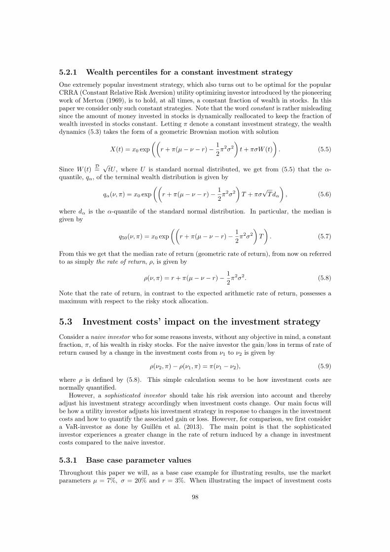
5.2.1 Wealth percentiles for a constant investment strategyOne extremely popular investment strategy, which also turns out to be optimal for the popularCRRA (Constant Relative Risk Aversion) utility optimizing investor introduced by the pioneeringwork of Merton (1969), is to hold, at all times, a constant fraction of wealth in stocks. In thispaper we consider only such constant strategies. Note that the word constant is rather misleadingsince the amount of money invested in stocks is dynamically reallocated to keep the fraction ofwealth invested in stocks constant. Letting π denote a constant investment strategy, the wealthdynamics (5.3) takes the form of a geometric Brownian motion with solution

X(t) = x0 exp

((r + π(µ− ν − r)− 1

2π2σ2

)t+ πσW (t)

). (5.5)

Since W (t)D=

√tU , where U is standard normal distributed, we get from (5.5) that the α-

quantile, qα, of the terminal wealth distribution is given by

qα(ν, π) = x0 exp

((r + π(µ− ν − r)− 1

2π2σ2

)T + πσ

√Tdα

), (5.6)

where dα is the α-quantile of the standard normal distribution. In particular, the median isgiven by

q50(ν, π) = x0 exp

((r + π(µ− ν − r)− 1

2π2σ2

)T

). (5.7)

From this we get that the median rate of return (geometric rate of return), from now on referredto as simply the rate of return, ρ, is given by

ρ(ν, π) = r + π(µ− ν − r)− 1

2π2σ2. (5.8)

Note that the rate of return, in contrast to the expected arithmetic rate of return, possesses amaximum with respect to the risky stock allocation.

5.3 Investment costs’ impact on the investment strategyConsider a naive investor who for some reasons invests, without any objective in mind, a constantfraction, π, of his wealth in risky stocks. For the naive investor the gain/loss in terms of rate ofreturn caused by a change in the investment costs from ν1 to ν2 is given by

ρ(ν2, π)− ρ(ν1, π) = π(ν1 − ν2), (5.9)

where ρ is defined by (5.8). This simple calculation seems to be how investment costs arenormally quantified.

However, a sophisticated investor should take his risk aversion into account and therebyadjust his investment strategy accordingly when investment costs change. Our main focus willbe how a utility investor adjusts his investment strategy in response to changes in the investmentcosts and how to quantify the associated gain or loss. However, for comparison, we first considera VaR-investor as done by Guillén et al. (2013). The main point is that the sophisticatedinvestor experiences a greater change in the rate of return induced by a change in investmentcosts compared to the naive investor.

5.3.1 Base case parameter valuesThroughout this paper we will, as a base case example for illustrating results, use the marketparameters µ = 7%, σ = 20% and r = 3%. When illustrating the impact of investment costs

98

we consider the difference between paying investment costs at rate ν1 = 1.4% and ν2 = 0.6%,respectively. Most papers focus on the impact of introducing investment costs. We focus onan individual who prefers to hand over the asset management to a fund. In that situation itseems unattainable to obtain zero investment costs. Therefore, we consider instead the “price” ofinvesting through an expensive fund (ν1) compared to a cheap fund (ν2). The investment costsconsidered are consistent with those observed in the market (see references in Section 5.1).

5.3.2 The Value at Risk approachThis subsection briefly presents and explains the impact of investment costs for a VaR-investor,as presented in Guillén et al. (2013). A VaR(α)-investor is an investor being concerned withthe value of the α-quantile of the terminal wealth distribution, i.e. with the level for which therealized terminal wealth risk to fall below with a probability of α-percent. Denote the lower levelof wealth by X(T ). To be more precise, the VaR(α)-investor facing investment costs ν1 chooseshis investment strategy, π1, such that

qα(ν1, π1) = X(T ), (5.10)

where qα is given by (5.6). The point is that if investment costs change from ν1 to ν2 this relationholds no more, i.e.

qα(ν2, π1) = X(T ). (5.11)

Obviously, the VaR-(α)-investor should adjust his investment strategy such that the VaR-criteria(5.11) is still fulfilled. We therefore look for a change in the investment strategy, ∆, fulfillingthe relation

qα(ν2, π1 +∆) = qα(ν1, π1), (5.12)

i.e. being faced with investment costs ν2 the investor should instead invest π2 = π1 + ∆ of hiswealth in risky stocks. We get the solution

∆ =−b±

√D

2a, (5.13)

where D = b2 − 4ac and

a =σ

2, (5.14)

b = −(µ− ν2 − r) + π1σ2 − σdα√

T, (5.15)

c = π1(ν2 − ν1). (5.16)

Of the two solutions we focus on the one allowing for more stocks in the case of lower costs (ν2 <ν1) and fewer stocks in the case of higher costs (ν2 > ν1). Guillén et al. (2013) derive restrictionson the parameter space ensuring that the median increases and the α-quantile decreases whenexposure in the risky asset increases. In contrast to (5.9) the change in rate of return becomes

ρ(ν2, π2)− ρ(ν1, π1) = π1(ν1 − ν2) + ∆(µ− ν2 − r)− 1

2∆2σ2 − π1∆σ

2. (5.17)

Note that since ∆ and π1 depend on the investment horizon so does the change in rate of re-turn. Figure 5.1 illustrates for the base case example (see Subsection 5.3.1) the VaR-calibrationconcept for an investor investing 1 unit initially. First, when investment costs are ν1 = 1.4%the VaR(10%)-investor chooses to invest π1 = 60% of his wealth in stocks corresponding toa 10-percent quantile for the terminal wealth distribution of q10%(ν1, 60%) = 1.75 and a me-dian of q50%(ν1, 60%) = 4.65. Not changing the investment strategy, but now being charged

99

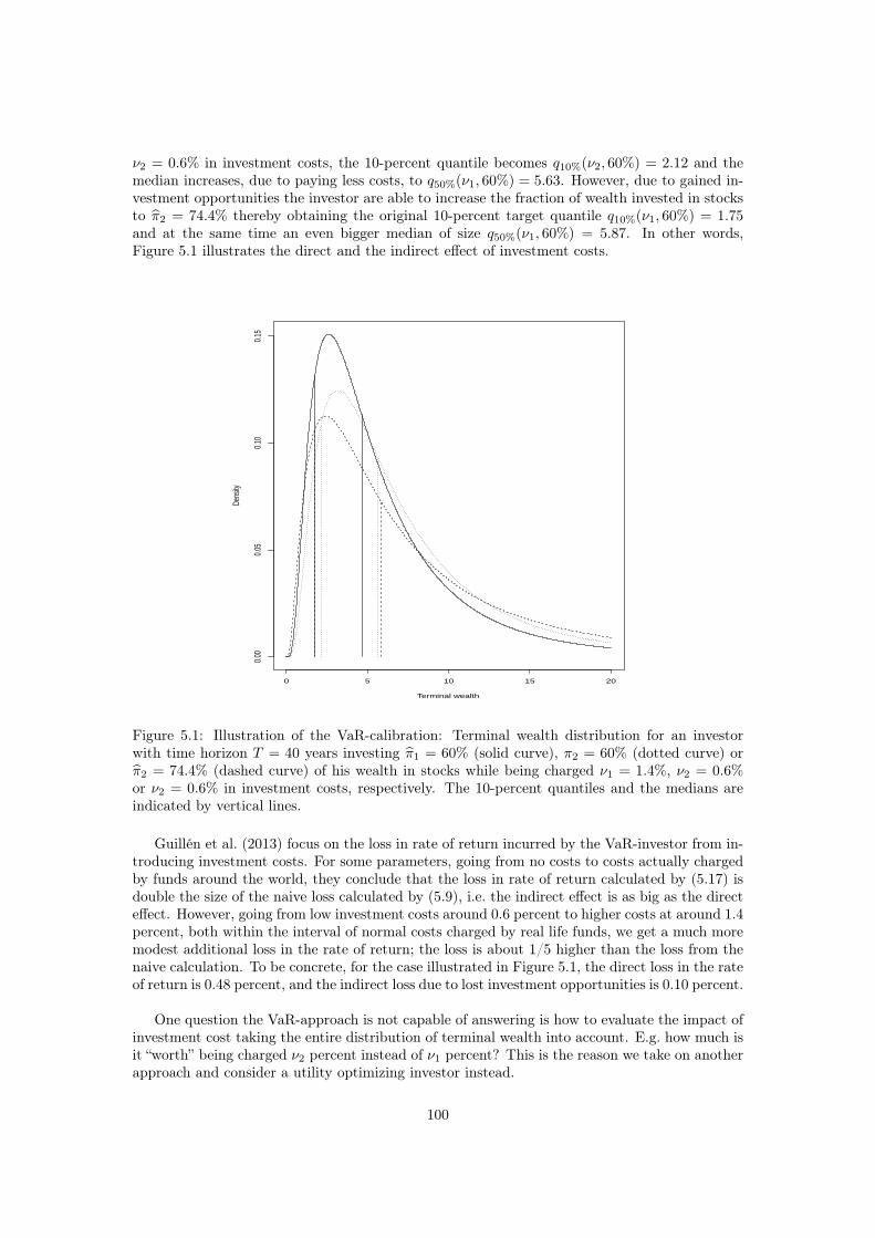
ν2 = 0.6% in investment costs, the 10-percent quantile becomes q10%(ν2, 60%) = 2.12 and themedian increases, due to paying less costs, to q50%(ν1, 60%) = 5.63. However, due to gained in-vestment opportunities the investor are able to increase the fraction of wealth invested in stocksto π2 = 74.4% thereby obtaining the original 10-percent target quantile q10%(ν1, 60%) = 1.75and at the same time an even bigger median of size q50%(ν1, 60%) = 5.87. In other words,Figure 5.1 illustrates the direct and the indirect effect of investment costs.

0 5 10 15 20

0.00

0.05

0.10

0.15

Terminal wealth

Dens

ity

Figure 5.1: Illustration of the VaR-calibration: Terminal wealth distribution for an investorwith time horizon T = 40 years investing π1 = 60% (solid curve), π2 = 60% (dotted curve) orπ2 = 74.4% (dashed curve) of his wealth in stocks while being charged ν1 = 1.4%, ν2 = 0.6%or ν2 = 0.6% in investment costs, respectively. The 10-percent quantiles and the medians areindicated by vertical lines.

Guillén et al. (2013) focus on the loss in rate of return incurred by the VaR-investor from in-troducing investment costs. For some parameters, going from no costs to costs actually chargedby funds around the world, they conclude that the loss in rate of return calculated by (5.17) isdouble the size of the naive loss calculated by (5.9), i.e. the indirect effect is as big as the directeffect. However, going from low investment costs around 0.6 percent to higher costs at around 1.4percent, both within the interval of normal costs charged by real life funds, we get a much moremodest additional loss in the rate of return; the loss is about 1/5 higher than the loss from thenaive calculation. To be concrete, for the case illustrated in Figure 5.1, the direct loss in the rateof return is 0.48 percent, and the indirect loss due to lost investment opportunities is 0.10 percent.

One question the VaR-approach is not capable of answering is how to evaluate the impact ofinvestment cost taking the entire distribution of terminal wealth into account. E.g. how much isit “worth” being charged ν2 percent instead of ν1 percent? This is the reason we take on anotherapproach and consider a utility optimizing investor instead.

100

5.3.3 The utility approachConsider an investor measuring his attitude towards risk by a constant relative risk aversion(CRRA) function defined by

u(x) =

xγ

γ , if x > 0,

limx0xγ

γ , if x = 0,

−∞, if x < 0,

(5.18)

for some γ ∈ (−∞, 1)\0 (γ = 0 corresponds to the logarithmic case). A commonly used objectfor the investor is to try maximizing the expected utility from terminal wealth. Formally, theinvestor looks for the investment strategy π∗ fulfilling

supπE [u(Xπ(T ))] = E

[u(Xπ∗

(T ))], (5.19)

where we have indicated the π-dependence of the terminal wealth in the notation. The problemgiven by (5.19) is one of the most well-known optimization problems from the literature offinancial stochastic control and is often referred to as Merton’s problem after the pioneering workof Merton (1969). The solution to the problem can be obtained by use of dynamic programming,which turns the stochastic optimization problem into a deterministic optimization problem anda set of partial differential equations (Hamilton-Jacobi-Bellman equations), or by use of themodern, more direct, method called the “Martingale method” developed by Cvitanic et al. (1987)and Cox and Huang (1989), which builds upon modern mathematical finance theory. Thesolution turns out to depend on the market price of risk, the investor’s risk aversion, and theinvestment costs, and is given by

π∗(ν) =1

1− γ

µ− ν − r

σ2. (5.20)

We see that the optimal investment strategy is to hold a constant fraction of wealth in riskyassets. This is a feature of CRRA utility which, from a mathematical point of view, is ratherappealing (see Subsection 5.2.1). The strategy itself dictates directly the change in the riskyposition induced by a change in investment costs. We get

∆ = π∗(ν2)− π∗(ν1) =1

1− γ

ν1 − ν2σ2

. (5.21)

As for the VaR-approach we see that, naturally, if the investment costs decrease (increase) morestocks should be bought (sold). However, opposed to the VaR-approach the change in the riskyposition is always unique (no short-selling solution). Even more appealing we get in contrastto the VaR-approach (see (5.17)) that the change in rate of return becomes independent of theinvestment horizon. We get, with π∗

i = π∗(νi), that

ρ(ν2, π∗2)− ρ(ν1, π

∗1) = π∗

1(ν1 − ν2) + ∆(µ− ν2 − r)− 1

2∆2σ2 − π∗

1∆σ2. (5.22)

Clearly, the rather large change in rate of return induced by lost/gained investment opportuni-ties, due to a change in investment costs, was for the VaR-investor partly because a very longinvestment horizon was considered. Since many private investors mainly invest through beinga member of a pension scheme, i.e. long time horizon, the conclusion still seems to be highlyrelevant. However, the fact that for the utility investor the change in rate of return inducedby a change in investment costs does not depend on the investment horizon counters criticismclaiming that the effect is negligible for short horizons.

Figure 5.2 illustrates for the base case example (see Subsection 5.3.1) the utility-calibrationconcept for an investor investing 1 unit initially. First, when investment costs are ν1 = 1.4% the

101

investor optimally invests π∗1 = 60% of his wealth in stocks. However, due to gained investment

opportunities the investor increases this fraction to π∗2 = 78.5% when investment costs decline to

ν2 = 0.6%. In contrast to the VaR-approach we see in Figure 5.2 that the 10-percent quantilesof the terminal wealth distributions are not equal for the two cases. The utility investor does notfocus solely on the 10-percent quantile, but evaluates the entire distribution of terminal wealthwhen he decides how much of the saved investment costs to invest in stocks. In this respect heacts more sophisticated than the VaR-investor.

0 5 10 15 20

0.00

0.05

0.10

0.15

Terminal wealth

Dens

ity

Figure 5.2: Illustration of the utility-calibration: Terminal wealth distribution for an investorwith time horizon T = 40 years investing π∗

1 = 60% (solid curve) or π∗2 = 78.5% (dashed

curve) of his wealth in stocks while being charged ν1 = 1.4% or ν2 = 0.6% in investment costs,respectively. The 10-percent quantiles and the medians are indicated by vertical lines.

5.3.4 Comparing the VaR and utility approachIn Subsections 5.3.2 and 5.3.3 we considered a VaR-investor and a utility optimizing investor,respectively. The VaR-investor picked his investment strategy in order to obtain a target 10-percent quantile for the terminal wealth distribution equal to 1.75. The utility investor pickedhis investment strategy in order to maximize expected utility from terminal wealth while usingthe power utility function given by (5.18) with risk aversion given by γ = −0.0833. In order to beable to compare the two investors’ reaction to changes in investment costs we have constructedthe two examples such that when investment costs are ν1 = 1.4% both investors prefer to investπ = 60% of the wealth in stocks.

Changing investment costs from ν1 = 1.4% to ν2 = 0.6% we saw in Subsections 5.3.2 and 5.3.3that the change in the investment strategy was ∆ = 14.4% for the VaR-investor and ∆ = 18.5%for the utility investor. From this example we conclude that the utility investor reacts morestrongly compared to the VaR-investor when investment costs change. However, as illustrated

102

by Figure 5.3, this is not a general rule of thumb. In fact, by changing the risk profiles suchthat both investors prefer a π = 30% position of wealth in stocks when investment costs areν1 = 1.4%, lowering the investment costs now makes the VaR-investor change his investmentstrategy more than the utility optimizing investor.

0.000 0.004 0.008 0.012

0.60

0.65

0.70

0.75

0.80

0.85

0.90

Investment costs (ν2)

Inves

tmen

t stra

tegy

(π2)

0.000 0.004 0.008 0.012

0.30

0.35

0.40

0.45

0.50

0.55

Investment costs (ν2)

Inves

tmen

t stra

tegy

(π2)

Figure 5.3: Illustrations of how the utility optimizing investor (solid curves) and the VaR-investor(dashed curves) change investment strategy when investment costs decrease from ν1 = 1.4% toν2 ∈ [0, ν1]. The left plot illustrates the case where the investors prefers a π = 60% allocation instocks, and the right plot the case of a preferable π = 30% allocation in stocks, when investmentcosts are ν1 = 1.4%. The dots indicate the base case example from earlier subsections whereinvestment costs decrease to ν2 = 0.06%. The investment horizon is T = 40.

5.4 Quantification of the impact of investment costsIn this section we use the utility approach described in Subsection 5.3.3 to quantify the impactof investment costs. Inserting the optimal investment strategy (5.20) into (5.5) we are able tocalculate the optimal expected utility given by (5.19). We get

supπE[u(X(ν,π)(T )

)]= E

[u(X(ν,π∗)(T )

)]=

1

γxγ0 exp

((r + π∗(µ− r − ν)− 1

2(π∗)

2σ2

)Tγ +

1

2(π∗)

2σ2γ2T

)=

1

γxγ0 exp

(r +

1

2

γ

1− γ

(µ− r − ν

σ

)2)T

, (5.23)

103

where x0 denotes the initial wealth. Now, define the Indifferent Compensation Ratio as theminimum relative increase in the initial wealth the investor demands in compensation to acceptincurring higher investment costs. Formally, the indifferent compensation ratio for two givenlevels of investment costs, ICR(ν1,ν2), is for v2 ≤ v1 given by the relation

supπE[u(X(ν2,π)(T )

) ∣∣∣X(ν2,π)(0) = x0

]= sup

πE[u(X(ν1,π)(T )

) ∣∣∣X(ν1,π)(0) = x0(1 + ICR(ν1,ν2)

)]. (5.24)

The certainty equivalent is the smallest amount of money the investor is willing to receivewith certainty at the horizon in exchange for the possibility to invest in the stock market. Informula, the certainty equivalent for a given level of investment costs, CEQ(ν), is defined by therelation

u(CEQ(ν)

)= sup

πE[u(X(ν,π)(T )

)]. (5.25)

Since by (5.5) the wealth process is linear in initial wealth we obtain

u(CEQ(ν2)

)= u

((1 + ICR(ν1,ν2)

)CEQ(ν1)

). (5.26)

From this we conclude that for power utility the two measures are equivalent in the sense that

CEQ(ν2) − CEQ(ν1)

CEQ(ν1)=

(1 + ICR(ν1,ν2)

)CEQ(ν1) − CEQ(ν1)

CEQ(ν1)= ICR(ν1,ν2), (5.27)

i.e. the relative change in certainty equivalents equals the indifferent compensation ratio. Thisis another appealing feature of power utility. Note that the indifferent compensation ratio givenby (5.24) can easily be calculated by (5.27) and (5.23).

We are now in a position to quantify the impact of investment costs using the indifferentcompensation measure given by (5.24). Consider the base case example of Subsection 5.3.1 withone unit initially invested and investment costs ν1 = 1.4% and ν2 = 0.6%, respectively. We get

ICR(ν1,ν2) =CEQ(ν2) − CEQ(ν1)

CEQ(ν1)=

5.66− 4.54

4.54= 0.248, (5.28)

i.e. the investor profits a gain equal to 24.8 percent of the initial wealth when investment costsdecrease from ν1 to ν2. In Subsection 5.3.2 we considered the change in rate of return induced bya change in investment costs and compared the naive change given by (5.9) with the change theVaR-investor experienced given by (5.17). For the utility optimizing investor it seems naturalto compare the indifferent compensation ratio with the present value of expected accumulatedinvestment costs over the horizon. In order to do so note that

d(e−rtX(t)) = −re−rtX(t)dt+ e−rtdX(t)

= e−rtX(t)π(µ− r − ν)dt+ e−rtX(t)πσdW (t), (5.29)

which implies

e−rTX(T ) = x0 +

∫ T

0

e−rtX(t)π(µ− r − ν)dt+

∫ T

0

e−rtX(t)πσdW (t). (5.30)

Taking expectation, noting that the wealth process is strictly positive, and using (5.5), we getthe following expression for the expected accumulated investment costs over the horizon.

adm(ν, π) ≡ E

[∫ T

0

e−rtX(t)πνdt

]= E[x0 − e−rTX(T ) +

∫ T

0

e−rtX(t)π(µ− r)dt]

= x0

(ν

µ− r − ν

)(eπ(µ−ν−r)T − 1

). (5.31)

104

From this we define the Relative present value of the Expected Change in accumulated investmentcosts induced by lowering investment costs from ν1 to ν2, REC(ν1,ν2), by

REC(ν1,ν2) ≡adm(ν1, π

∗1)− adm(ν2, π

∗2)

x0. (5.32)

Note that, as is the case for the indifferent compensation ratio, this value is independent of thesize of the initial wealth. We interpret (5.32) as the direct effect and the difference between (5.27)and (5.32) as the indirect effect of investment costs. The left plot in Figure 5.4 compares theindifferent compensation ratio (5.27) with (5.32) for different investment costs. In other words,we compare the size of the compensation sum with the expected accumulated investment costsover the horizon, relative to the size of the initial wealth. For the base case example (ν∗1 , ν

∗2 ) =

(1.4%, 0.6%) with corresponding optimal investment strategies (π1, π2) = (60%, 78.4%) we get

REC(ν1,ν2) = 0.467− 0.337 = 0.130, (5.33)

i.e. 13 percent of the initial wealth is expected to be used to pay for the extra investment costs.In contrast, we got in (5.28) that the investor demands an increase of 24.8% of initial wealthin compensation to accept incurring the higher investment costs ν1 = 1.4% instead of the lowerν2 = 0.6%. The great gap between these two values (the indirect effect) is due to the risk aver-sion of the utility investor. The “fear” that the actual amount of money spent on investmentcosts exceeds the expectation is overwhelming compared to the “benefit” that it is below. Thisis exactly what most analyses seem to forget. The fact that for reasonable values of investmentcosts the effect of higher costs seems to double is quiet surprising. As mentioned, one could referto the phenomenon as The double blow of investment costs. Clearly, one wonders how much thisdouble effect is due to the long horizon (T=40) considered by the base case example. The rightplot in Figure 5.4 illustrates that the effect is substantial even for a short term investor. Still,for a myopic investor the indirect effect is half the size of the direct effect.

Finally we analyze the relative importance of the investment strategy and investment costs.Specifically, we consider a power utility optimizing investor who hands over his savings to a fundcharging him high investment costs at a rate ν1. In return, the fund offers a tailored investmentstrategy π∗

1 fitted to meet the risk preferences of the client, i.e. the object given by (5.19)is optimized. The investor now becomes aware that another fund offers to manage his savingswhile only charging him investment costs at a lower rate ν2. However, in order to offer this cheapproduct, the fund is organized as an investment collective meaning that all members follow thesame investment strategy π2. Obviously, if the common investment strategy π2 exercised by thecheap fund happens to equal the tailored optimal investment strategy π∗

2 it’s a no-brainer —the investor should move to the cheap fund. However, how much can the collective investmentstrategy π2 offered by the cheap fund differ from the optimal tailored investment strategy π∗

2

while still being preferable for the investor to move to the cheap fund? In formula, we look forthe investment strategies π2 satisfying the relation

u(CEQ(ν1)

)= E

[u(X(ν2,π2)(T )

)]. (5.34)

By use of (5.23) we get the solution

π2 =−b±

√D

2a, (5.35)

where D = b2 − 4ac and

a =σ

2γ(1− γ), (5.36)

b = −(µ− ν2 − r), (5.37)

c =1

2

γ

1− γ

(µ− v1 − r

σ2

)2

. (5.38)

105

0.000 0.004 0.008 0.012

0.0

0.1

0.2

0.3

0.4

0.5

Investment costs (ν2)

ICR

and

REC

0 10 20 30 40

1.5

1.6

1.7

1.8

1.9

Investment horizon (T)

ICR

/ REC

Figure 5.4: Illustrations of the indifferent compensation ratio (ICR) and the relative presentvalue of the expected change in accumulated investment costs (REC). The left plot illustratesfor a fixed horizon T = 40 the values when investment costs decreases from ν1 = 1.4% toν2 ∈ [0, ν1] (ICR solid curve, REC dashed curve). The dots indicate the base case example fromearlier subsections where investment costs decrease to ν2 = 0.06%. The right plot illustrates fora decrease in investment costs from ν1 = 1.4% to ν2 = 0.6% the proportion between the twomeasures (ICR/REC) for varying time horizons.

Note that the solution does not depend on the investment horizon.The right-most curve in Figure 5.5 illustrates, for the parameters (ν1, π∗

1) = (1.4%, 60%) andν2 ∈ [0, ν1], the cost-dependent value of π2 for which the investor is indifferent between the twofunds. From left to right the next 5 curves illustrates cost-dependent values of π2 for whichthe investor is 10, 20, 30, 40 and 50 percent better off being a member of the cheaper fund.The line illustrates the cost-dependent optimal risk allocation π∗

2 . The conclusion is surprisinglyclear. If the investor is offered the lower cost rate ν2 = 0.6% instead of the higher cost rateν1 = 1.4%, he is better off almost no matter how much the investment strategy differs from hisrisk preferences. Any investment strategy π2 ∈ (0.28, 1.29) makes the cheaper fund preferable(remember π∗

2 = 78.5% is optimal). As seen in Figure 5.5 this interval shrinks when consideringscenarios where the investor is 10, 20, 30, 40 and 50 percent better off. Still, the range ofinvestment strategies are incredible large. Once again, the conclusion, which is independentof the investment horizon, is very clear: The investor should be much more concerned withinvestment costs compared to being concerned with which investment strategy exactly meets hisrisk preferences.

106

0.000 0.002 0.004 0.006 0.008 0.010 0.012 0.014

0.2

0.4

0.6

0.8

1.0

1.2

1.4

1.6

Investment costs (ν2)

Inves

tmen

t stra

tegy

(π2)

Figure 5.5: The curves illustrate for given investment costs ν2 ∈ [0, ν1] the investment strategiesπ2 which makes the investor (from right to left) 0, 10, 20, 30, 40 and 50 percent better offcompared to being charged ν1 = 1.4% while using the optimal investment strategy π∗

1 = 60%.The line illustrates the cost-dependent optimal stock allocation.

107

108

6. Entrance times of random walks: Withapplications to pension fund modeling

Abstract: The purpose of the paper is twofold. First, we consider entrance timesof random walks, i.e. the time of first entry to the negative axis. Partition sum for-mulas are given for entrance time probabilities, the nth derivative of the generatingfunction, and the nth falling factorial entrance time moment. Similar formulas for thecharacteristic function of the position of the random walk both conditioned on entryand conditioned on no entry are also established. Second, we consider a model for awith-profits collective pension fund. The model has previously been studied by ap-proximate methods, but we give here an essentially complete theoretical descriptionof the model based on the entrance time results. We also conduct a mean-varianceanalysis for a fund in stationarity. To facilitate the analysis we devise a simple andeffective exact simulation algorithm for sampling from the stationary distribution of aregenerative Markov chain.

Keywords: Random walks, entrance times, generating function, factorial moment,partition sum, stationarity, exact simulation, collective pension fund, with-profits con-tracts.

6.1 IntroductionThis paper analyzes a “with-profits collective pension scheme”; this type of scheme and variantshereof are widespread, among other places, in the Nordic countries and the Netherlands. Mem-bers of the scheme are guaranteed a minimum benefit. The guarantees are a liability for thepension fund for which it must reserve an amount of money equal to the net present value offuture guaranteed benefits (the reserve). In addition to the already guaranteed benefits mem-bers may receive bonus in the form of increased guarantees. Bonus is attributed periodically,e.g. annually, when the ratio of total assets to the reserve (the funding ratio) is sufficiently high.The phrase “with-profits” refers to this profit-sharing mechanism.

Assets in excess of the reserve are termed the bonus potential. The bonus potential allows thefund to invest in risky assets by absorbing adverse investment results. The scheme is “collective”in the sense that the bonus potential is considered common to all members. It is also collective inthe sense that the investment strategy and bonus policy is the same for all members. Collectivefunds generally benefit from economy of scale in the form of low administration and investmentcosts. The flip side is the lack of an individual investment strategy.

We consider a model for a collective pension fund in which bonus is attributed when thefunding ratio exceeds a given bonus threshold. The fund follows a CPPI (Constant ProportionPortfolio Insurance) investment strategy in order to stay solvent, i.e. to ensure that total assetsexceed the reserve. The paper gives an essentially complete description of the fund dynamicsincluding the time between bonuses, the (conditional) expected bonus percentage and the (con-ditional) expected funding ratio. The analysis is based on a detailed study of an embeddedone-sided random walk obtained by a transformation of the funding ratio process sampled atthe discrete set of time points where bonus can be attributed. We consider both a fund startingat the bonus threshold and a fund in stationarity. Furthermore, we use the results to perform amean-variance analysis of a standardized benefit payout. The analysis is performed for a fundin stationarity representing the “average” member. To facilitate the analysis we also employ an

109

exact simulation algorithm, which might be of independent interest.

The theoretical foundation for the analysis is a series of new results for entrance times ofrandom walks derived in this paper. For a random walk started at the origin the entrance timeis the time of entry into (−∞, 0]. The main theoretical results are partition sum formulas for thenth derivative of the entrance time generating function and for the nth falling factorial entrancetime moment. The latter result generalizes the well-known formula for the mean entrance time.We also give a partition sum formula for entrance time probabilities, and a similar formula forthe position of the random walk conditioned on entrance at time n. These results are implicitin Spitzer (1956) and Asmussen (2003), but the proofs are new and simpler. Finally, we give anew partition sum formula for the position of the random walk conditioned on entrance takenplace after time n.

The results allow explicit calculations of the entrance time probabilities and moments in termsof the marginal distribution of the random walk. The computational effort gradually becomesprohibitive, but the first 100, say, entrance time probabilities and moments are computationallyfeasible. We use the results to study the one-sided random walk embedded in the funding ra-tio process by utilizing the fact that a one-sided random walk and its associated (unrestricted)random walk are identical up to the time of first entry into (−∞, 0]. However, the results aregenerally applicable and not limited to our pension fund application.

Optimizing utility from terminal wealth for an individual saving for retirement is treated bynumerous papers. The foundation was laid by Richard (1975) and to mention a few, who amongother results obtain optimal investment strategies, there is, Huang and Milevsky (2008) who allowfor unspanned labor income; Huang et al. (2008) who separate the breadwinner income processfrom the family consumption process; Steffensen and Kraft (2008) who generalize to a multi-state Markov chain framework typically used by actuaries for modeling a series of life historyevents; Bruhn and Steffensen (2011) who generalize to a multi-person household, with focus ona married couple with economically and/or probabilistically dependent members; Kwak et al.(2011) who also consider a household but focus on generation issues; Kronborg and Steffensen(2013) who calculate the optimal investment strategy for a pension saver in the present of aminimum rate guarantee; and Gerber and Shiu (2000) who present a comprehensive discussionof terminal utility optimization in a pension saving context. There is also a vast literature onmodern investment management, founded by Markowitz (1952) and Merton (1971), aimed atfinding optimal investment strategies without the pension aspect.

In contrast to the literature cited above this paper takes the point of view of a pensionfund where a group of people share a common investment strategy. Investment gains are sharedthrough a bonus strategy by which collective funds above a threshold are transferred to individualguarantees. Based on results on utility optimization of durable goods by Hindi and Huang (1993)it can be shown that the optimal bonus strategy is to continuously attribute bonus whenever thefunding ratio exceeds a certain barrier — thereby not allowing the funding ratio to exceed thebarrier. In this paper, and in real life, the transfer is done periodically rather than continuously.References for continuous-time analysis of pension schemes taking both assumed (technical)returns, realized returns and bonus into account include Norberg (1999), Steffensen (2000),Norberg (2001), Steffensen (2004) and Nielsen (2006).

We assume the fund to follow a CPPI strategy. This strategy ensures that the fund remainsfunded, and it is “locally” optimal if we consider the periods between possible bonus attributionsas local horizons. More precisely, Preisel et al. (2010) point out that CPPI is optimal in a finitehorizon setting with HARA-utility and a subsistence level corresponding to a terminal fundingratio of one. CPPI strategies are treated, for the unrestricted case, by Cox and Huang (1989),and for the restricted case, by Teplá (2001). Using a CPPI strategy, and thereby avoiding insol-vency, as done in this paper, stands in contrast to the literature on constructing contracts thatare fair between owners and policyholders, see e.g. Briys and de Varenne (1997) and Grosen andJørgensen (2000).

110

The current paper is related to Preisel et al. (2010), Kryger (2010) and Kryger (2011). We usethe same underlying funding ratio dynamics, but the pension product and the terms by whichmembers enter and leave the fund differ. In the cited papers members pay a fixed share (possiblyzero) of contributions to the bonus potential on entry. This raises a number of issues regardingintergenerational fairness. In the present setup the share depends on the funding status of thefund in such a way that the contract is always financially fair. Methodologically, the cited papersuse various analytical approximations while the current paper relies almost exclusively on exactresults.

The main insight of Preisel et al. (2010) is that a given year’s apparent success of a largebonus resulting from a high equity allocation can come at the even higher price of subsequentlarge losses trapping the company at a low funding ratio for a long period. They also deriveapproximations to the expected bonus and funding ratio in stationarity. Kryger (2010) findsoptimal investment strategies for power utility and mean-variance criteria. For fixed values ofthe bonus threshold, he finds optimal investment strategies in the class of CPPI strategies for afund in stationary. It is found that different investment strategies imply only modest differencesin utility and, hence, that an investment collective can accommodate quite different attitudestowards risk. Finally, Kryger (2011) studies the impact of the pension design on efficiency andintergenerational fairness.

The rest of the paper is organized as follows. Section 6.2 presents the theoretical contributionson entrance times and moments of random walks. Section 6.3 describes the pension fund model,and Section 6.4 applies the random walk results to study bonus waiting times, size of bonus andthe funding ratio. Results are given for a fund started at the bonus threshold and for a fundin stationarity. Section 6.5 contains a comprehensive numerical application including a mean-variance analysis. It also explains the exact simulation algorithm used in the analysis. Finally,the appendix contains proofs for the results of Section 6.2 and additional lemmas.

6.2 Random walksIn this section we present a series of results on entrance times and conditional characteristicfunctions of random walks. The results will be used in subsequent sections to provide a detaileddescription of the distribution of bonus times, size of bonus and funding ratio of the collectivepension fund model under study. However, the results are generally applicable and can beapplied in many other contexts as well.

The entrance time of a random walk is defined as the (first) time of entry into (−∞, 0] aftertime 0. The results to follow devise how a number of quantities related to entrance times canbe computed as sums over partition sets. We present both new results and existing results withnew and simpler proofs. The results fall in three parts.

First, we derive a closed-form formula for the entrance time probabilities of a random walkstarted at the origin (Theorem 6.2.3). This result is also implicit in the seminal paper by Spitzer(1956), but we give here a simpler self-contained proof. Second, we derive an expression forthe nth derivative of the generating function for the entrance time (Theorem 6.2.5), which wesubsequently use to derive a formula for the factorial moments (Theorem 6.2.6). These results arenew. Third, we derive formulas for the characteristic function of the position of the random walkconditioned on entrance at time n (Theorem 6.2.8) and on entrance after time n (Theorem 6.2.9).The first of these results is known, but the proof is new, while the second result is new. Most ofthe proofs rely on combinatorial arguments, some of which might be of independent interest, inparticular Lemma 6.6.1.

111

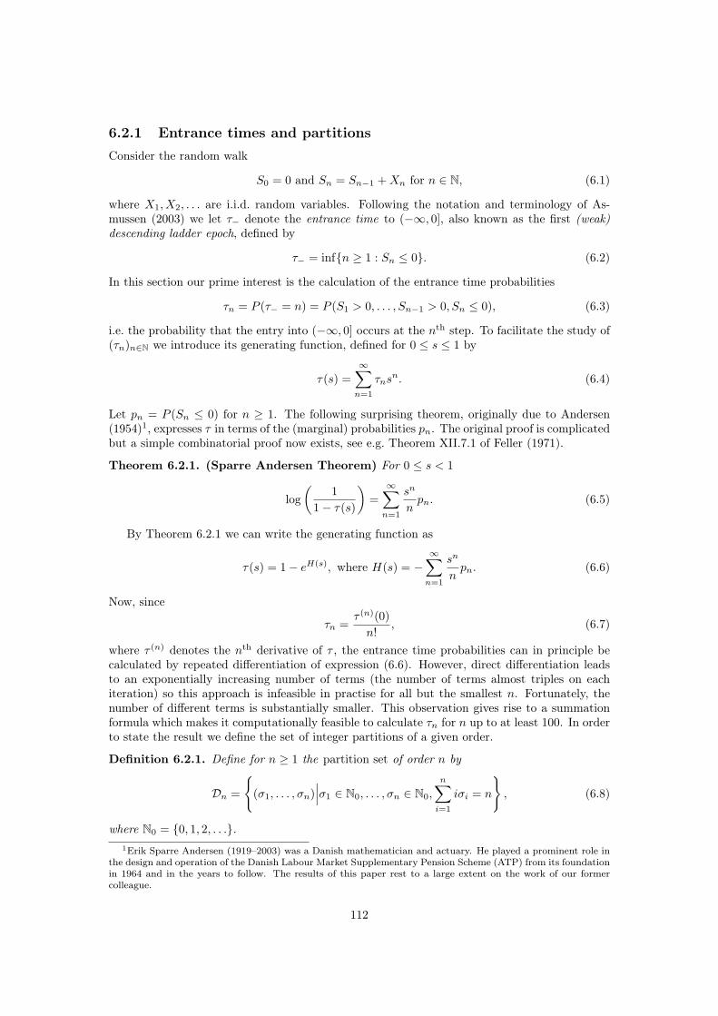
6.2.1 Entrance times and partitionsConsider the random walk

S0 = 0 and Sn = Sn−1 +Xn for n ∈ N, (6.1)

where X1, X2, . . . are i.i.d. random variables. Following the notation and terminology of As-mussen (2003) we let τ− denote the entrance time to (−∞, 0], also known as the first (weak)descending ladder epoch, defined by

τ− = infn ≥ 1 : Sn ≤ 0. (6.2)

In this section our prime interest is the calculation of the entrance time probabilities

τn = P (τ− = n) = P (S1 > 0, . . . , Sn−1 > 0, Sn ≤ 0), (6.3)

i.e. the probability that the entry into (−∞, 0] occurs at the nth step. To facilitate the study of(τn)n∈N we introduce its generating function, defined for 0 ≤ s ≤ 1 by

τ(s) =∞∑

n=1

τnsn. (6.4)

Let pn = P (Sn ≤ 0) for n ≥ 1. The following surprising theorem, originally due to Andersen(1954)1, expresses τ in terms of the (marginal) probabilities pn. The original proof is complicatedbut a simple combinatorial proof now exists, see e.g. Theorem XII.7.1 of Feller (1971).

Theorem 6.2.1. (Sparre Andersen Theorem) For 0 ≤ s < 1

log

(1

1− τ(s)

)=

∞∑n=1

sn

npn. (6.5)

By Theorem 6.2.1 we can write the generating function as

τ(s) = 1− eH(s), where H(s) = −∞∑

n=1

sn

npn. (6.6)

Now, since

τn =τ (n)(0)

n!, (6.7)

where τ (n) denotes the nth derivative of τ , the entrance time probabilities can in principle becalculated by repeated differentiation of expression (6.6). However, direct differentiation leadsto an exponentially increasing number of terms (the number of terms almost triples on eachiteration) so this approach is infeasible in practise for all but the smallest n. Fortunately, thenumber of different terms is substantially smaller. This observation gives rise to a summationformula which makes it computationally feasible to calculate τn for n up to at least 100. In orderto state the result we define the set of integer partitions of a given order.

Definition 6.2.1. Define for n ≥ 1 the partition set of order n by

Dn =

(σ1, . . . , σn)

∣∣∣σ1 ∈ N0, . . . , σn ∈ N0,

n∑i=1

iσi = n

, (6.8)

where N0 = 0, 1, 2, . . ..1Erik Sparre Andersen (1919–2003) was a Danish mathematician and actuary. He played a prominent role in

the design and operation of the Danish Labour Market Supplementary Pension Scheme (ATP) from its foundationin 1964 and in the years to follow. The results of this paper rest to a large extent on the work of our formercolleague.

112

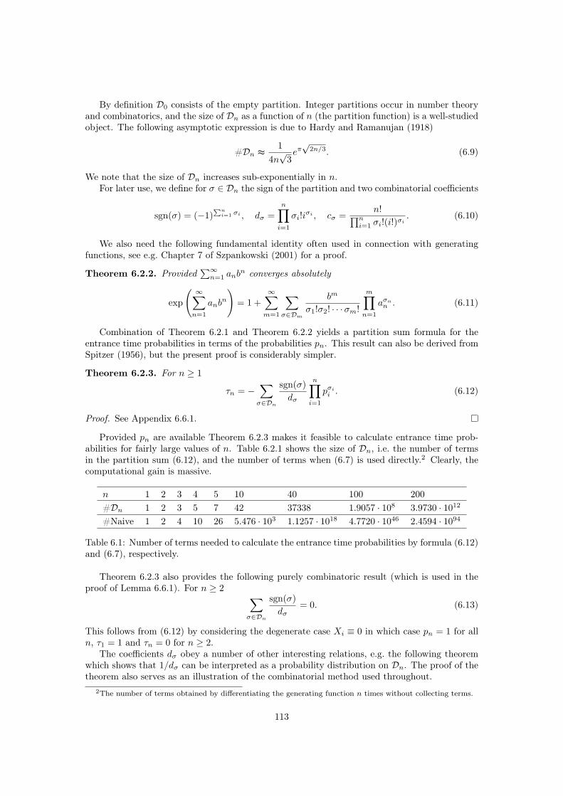
By definition D0 consists of the empty partition. Integer partitions occur in number theoryand combinatorics, and the size of Dn as a function of n (the partition function) is a well-studiedobject. The following asymptotic expression is due to Hardy and Ramanujan (1918)

#Dn ≈1

4n√3eπ√

2n/3. (6.9)

We note that the size of Dn increases sub-exponentially in n.For later use, we define for σ ∈ Dn the sign of the partition and two combinatorial coefficients

sgn(σ) = (−1)∑n

i=1 σi , dσ =n∏

i=1

σi!iσi , cσ =

n!∏ni=1 σi!(i!)

σi. (6.10)

We also need the following fundamental identity often used in connection with generatingfunctions, see e.g. Chapter 7 of Szpankowski (2001) for a proof.

Theorem 6.2.2. Provided∑∞

n=1 anbn converges absolutely

exp

( ∞∑n=1

anbn

)= 1 +

∞∑m=1

∑σ∈Dm

bm

σ1!σ2! · · ·σm!

m∏n=1

aσnn . (6.11)

Combination of Theorem 6.2.1 and Theorem 6.2.2 yields a partition sum formula for theentrance time probabilities in terms of the probabilities pn. This result can also be derived fromSpitzer (1956), but the present proof is considerably simpler.

Theorem 6.2.3. For n ≥ 1

τn = −∑σ∈Dn

sgn(σ)

dσ

n∏i=1

pσii . (6.12)

Proof. See Appendix 6.6.1.

Provided pn are available Theorem 6.2.3 makes it feasible to calculate entrance time prob-abilities for fairly large values of n. Table 6.2.1 shows the size of Dn, i.e. the number of termsin the partition sum (6.12), and the number of terms when (6.7) is used directly.2 Clearly, thecomputational gain is massive.

n 1 2 3 4 5 10 40 100 200#Dn 1 2 3 5 7 42 37338 1.9057 · 108 3.9730 · 1012

#Naive 1 2 4 10 26 5.476 · 103 1.1257 · 1018 4.7720 · 1046 2.4594 · 1094

Table 6.1: Number of terms needed to calculate the entrance time probabilities by formula (6.12)and (6.7), respectively.

Theorem 6.2.3 also provides the following purely combinatoric result (which is used in theproof of Lemma 6.6.1). For n ≥ 2 ∑

σ∈Dn

sgn(σ)

dσ= 0. (6.13)

This follows from (6.12) by considering the degenerate case Xi ≡ 0 in which case pn = 1 for alln, τ1 = 1 and τn = 0 for n ≥ 2.

The coefficients dσ obey a number of other interesting relations, e.g. the following theoremwhich shows that 1/dσ can be interpreted as a probability distribution on Dn. The proof of thetheorem also serves as an illustration of the combinatorial method used throughout.

2The number of terms obtained by differentiating the generating function n times without collecting terms.

113

Theorem 6.2.4. For n ≥ 1 and 1 ≤ k ≤ n∑σ∈Dn

1

dσ=∑σ∈Dn

kσkdσ

= 1. (6.14)

6.2.2 Entrance time momentsIn principle the entrance time moments (and other characteristics) can be calculated from theentrance time probabilities, τn. However, since the calculation of τn becomes increasingly diffi-cult it is both theoretically and practically important to have more direct means of calculatingmoments. In this section we present a formula for the falling factorial entrance time moments.This result generalizes the well-know formula for the mean entrance time3

E(τ−) = exp

( ∞∑k=1

1

kP (Sk > 0)

). (6.15)

The formula for the factorial moments rely on the following main result which gives a partitionsum representation of the nth derivative of the generating function. We denote by f (n) the nth

derivative of a function f .

Theorem 6.2.5. For n ≥ 1 and 0 ≤ s < 1

τ (n)(s) = −eH(s)∑σ∈Dn

cσHσ(s), (6.16)

where cσ is given by (6.10) and

Hσ(s) =n∏

i=1

(H(i)(s)

)σi

. (6.17)

Proof. See Appendix 6.6.2.

Note that Theorem 6.2.3 can be derived from Theorem 6.2.5 since τn = τ (n)(0)/n! andH(i)(0) = −(i − 1)!pi. This constitutes an alternative proof of Theorem 6.2.3 which does notrely on Theorem 6.2.2.

For integers m and n we denote by (m)n the nth falling factorial of m,

(m)n = m(m− 1) · · · (m− n+ 1). (6.18)

In particular, (m)1 = m and (m)n = 0 for n > m. By monotone convergence the nth factorialmoment of τ− is given by

E((τ−)n) = lims→1−

τ (n)(s), (6.19)

whether or not the limit is finite. Using Theorem 6.2.5 and (6.19) in combination with Lem-mas 6.6.1 and 6.6.2 the following result for the nth factorial moment can be derived.

Theorem 6.2.6. If n ≥ 1 and∑∞

k=1 kn−2P (Sk > 0) <∞ then

E((τ−)n) = exp

( ∞∑k=1

1

kP (Sk > 0)

)n!

∑σ∈Dn−1

n−1∏i=1

(hii!

)σi 1

σi!<∞, (6.20)

where, for n = 1, the last sum is 1 by definition, and for 1 ≤ i ≤ n− 1

hi =∞∑k=i

(k)ikP (Sk > 0). (6.21)

3Expression (6.15) can be derived from Theorem 6.2.1 by a limit argument, see e.g. Theorem XII.7.3 of Feller(1971).

114

Proof. See Appendix 6.6.2.

By use of Theorem 6.2.6 we can calculate entrance time moments of any order. For the firstthree moments we get

E (τ−) = exp

( ∞∑k=1

qkk

), (6.22)

E(τ2−)= E((τ−)2) + E(τ−) = E (τ−)

(2

∞∑k=1

qk + 1

), (6.23)

E(τ3−)= E((τ−)3) + 3E((τ−)2) + E(τ−)

= E (τ−)

(3

∞∑k=2

(k − 1)qk + 3∞∑k=1

qk

[ ∞∑k=1

qk + 2

]+ 1

), (6.24)

where qk = 1 − pk = P (Sk > 0). These formulas are all easy to evaluate to any desired degreeof accuracy.

6.2.3 Conditional characteristic functionsIn this section we present results characterizing the position of the random walk upon entranceto (−∞, 0] (the weak descending ladder height) and the position when entrance has not yetoccurred. We will need the combined generating and characteristic function defined for |s| < 1and ζ ∈ R by

χ(s, ζ) = E(sτ−eiζSτ−

). (6.25)

For a random variable X and an event A we write E(X;A) for E(X1A), and E(X|A) forE(X1A)/P (A). From Theorem VII 4.1 of Asmussen (2003) we have the following generalizationof Theorem 6.2.1

Theorem 6.2.7. For |s| < 1 and ζ ∈ R

log

(1

1− χ(s, ζ)

)=

∞∑n=1

sn

nE(eiζSn ;Sn ≤ 0

). (6.26)

By combining Theorem 6.2.7 and Theorem 6.2.2 we obtain a partition sum formula for thecharacteristic function of the random walk given entrance to (−∞, 0] at time n. This result issimilar to Theorem 6.2.3 for the entrance time probabilities.

Theorem 6.2.8. For n ≥ 1 and ζ ∈ R

E(eiζSn |τ− = n

)= − 1

τn

∑σ∈Dn

sgn(σ)

dσ

n∏k=1

(E(eiζSk ;Sk ≤ 0

))σk. (6.27)

Proof. See Appendix 6.6.3.

It is also of interest to know the distribution of the random walk given that it has not yetentered (−∞, 0]. It turns out that the characteristic function for this distribution can alsobe calculated as a partition sum. The result is established by subtracting the characteristicfunction of Theorem 6.2.8 up to time n from the unconditional characteristic function and usingLemma 6.6.1 to identify the resulting structure.

115

Theorem 6.2.9. For n ≥ 1 and ζ ∈ R

E(eiζSn |τ− > n) =1

P (τ− > n)

∑σ∈Dn

1

dσ

n∏k=1

(E(eiζSk ;Sk > 0)

)σk. (6.28)

Proof. See Appendix 6.6.3.

Note that if P (τ− < ∞) = 1 then P (τ− > n) = 1 −∑n

i=1 τi such that (6.28) can indeed becalculated.

6.3 Pension fund modelWe consider a model for a collective pension fund with a with-profits pension product. Eachcontribution is split into a part giving a guaranteed payment and a part invested in a, possiblyleveraged, investment portfolio. The product is with-profit in the sense that all guaranteed pay-ments are increased, known as bonus, when the funding ratio exceeds a given threshold level.The investment strategy and bonus policy are common and all members receive the same bonus(percentage). In our model members enter and leave the fund on financially fair terms, althoughthis is not necessarily strictly true in practice. Despite its simplicity the model resembles thetraditional collective pension funds known from e.g. the Nordic countries and the Netherlands.The random walk results presented in Section 6.2 will be used to give an essentially completedescription of the dynamics of the fund.

First, consider a frictionless Black-Scholes market consisting of a bank account, B, with riskfree short rate, r, and a risky stock, S, with dynamics given by

dB(t) = rB(t)dt, B(0) = 1, (6.29)dZ(t) = (r + µ)Z(t)dt+ σZZ(t)dW (t), Z(0) = z0 > 0. (6.30)

Here r, µ and σZ are strictly positive constants. The process W is a standard Brownian motionon the probability space (Ω,F ,P) equipped with the filtration FW = (FW (t))t≥0 given by theP -augmentation of the filtration (σW (s); 0 ≤ s ≤ t)t≥0.

The decision to attribute bonus or not is taken at a set of equidistant, discrete set of timepoints 0 = t0 < t1 < . . .. We assume for simplicity that contributions and benefits also fall atthese times. The market value of the guaranteed benefits, the reserve, is denoted R(t). Nottaking mortality into account (paramount to assuming that mortality risk can be neglected bythe law of large numbers) the evolution of the reserve between potential bonus times is given by

R(t) = R(ti)er(t−ti), where i = maxj ∈ N0 : tj ≤ t. (6.31)

The total assets of the fund is denoted A(t) and the funding ratio of the fund is defined as

F (t) =A(t)

R(t). (6.32)

The difference between total assets and the reserve, A(t) − R(t), is called the bonus potential(or surplus). We assume that the fund attributes bonus according to a threshold bonus strategysuch that at time ti all guaranteed payments are increased by

rBi =

0 if F (ti−) ≤ κ,F (ti−)−κ

κ if F (ti−) > κ,(6.33)

where κ is assumed to be strictly larger than 1. Note that immediately after a bonus attributionthe funding ratio equals κ. Let Fi denote the funding ratio at time ti after (possible) bonus

116

attribution, but before contributions and benefits have fallen. Thus Fi = F (ti−)/(1 + rBi ) =minF (ti−), κ.

The pension product:

• Contributions do not affect the funding ratio, i.e. for contributions received at time ti onlythe fraction 1/Fi is guaranteed (at rate r) and enters to the reserve while the remainderenters to the bonus potential.

• The initially guaranteed benefit is entitled to bonus from the time of contribution to thetime of payment.

• Benefits do not affect the funding ratio, i.e. guaranteed benefits paid out at time ti areincreased by Fi (terminal bonus).

Note that the fraction of contributions guaranteed at the risk-free rate4 depends on thecurrent funding ratio of the fund. Also note that for each contribution the member pays a priceto enter the collective fund, but he also receives his share of the surplus for each benefit paidout.

Let ci and bi denote the contributions and benefits, respectively, at time ti, and let cGi andbGi denote the part of contributions and benefits guaranteed. Total assets and the reserve attime ti is then given by

A(ti) = A(ti−) + ci − bi, (6.34)

R(ti) =(1 + rBi

)R(ti−) + cGi − bGi , (6.35)

where cGi = ci/Fi and bGi = bi/Fi. Hence, by construction F (ti) = Fi irrespective of the sizeof contributions and benefits. It is not hard to show that the fact that pension savers enterand leave the pension fund without effecting the funding ratio makes the scheme financially fair.There is no redistribution of wealth between generations.

The simplest pension product to be considered is the case in which a contribution of one ismade at time t = 0 for a benefit paid out in its entirety at t = T (retirement). In this case thebenefit at retirement becomes

OT =F (T )

F (0)erT

T∏i=1

(1 + rBi

). (6.36)

Different contribution and benefit profiles can also be analyzed within this model. The point tonote is that the payoff depends solely on the funding ratio dynamics.

We assume that the pension fund has to stay funded at all times, i.e. its assets must notfall below the reserve or, equivalently, the funding ratio must not fall below one. In order toachieve this the fund pursues a CPPI (constant proportion portfolio insurance) strategy by whicha constant fraction, C, of the bonus potential is invested in stocks. The remaining assets areinvested in the risk-free asset. We allow for values of C greater than one, i.e. leverage of thebonus potential is possible. The dynamics of the assets between time ti and ti+1 is given by

dA(t) = (r + γ(t)µ)dt+ γ(t)σZdW (t), (6.37)

where γ(t) = C F (t)−1F (t) .

Let ∆ denote the time between possible bonus attributions, ti = i∆, and let Fi = F (ti).It follows from Preisel et al. (2010)) that the funding ratio process sampled at ti evolves live a(discrete-time) Markov chain with dynamics

Fi = min(Fi−1 − 1)e(Cµ− 1

2C2σ2

Z)∆+CσZ

√∆Ui + 1, κ

, (6.38)

4We disregard throughout mortality and the associated mortality bequest from the deceased to the survivorswhich acts as an increased rate of return in the case of life annuities.

117

where the Ui’s are i.i.d. standard normal variables. In particular, if F0 > 1 all subsequent Fi’sare strictly larger than 1 (and at most κ).

The fund has to decide on an investment strategy, C, and a bonus policy, κ. A high bonusthreshold implies that the fund can invest more freely but also that only a small fraction ofthe pension is guaranteed. This may or may not be in the interest of the members. Similarly,an aggressive investment strategy implies a higher probability of very high returns, but also ahigher risk of very low returns (on the bonus potential).

The purpose of the rest of the paper is twofold. First, we characterize the impact of C andκ in terms of bonus time (time between bonus attributions), bonus size and funding ratio. Thecharacterization is provided for funds started at κ and in stationarity (the long-run average).Second, we propose a criterion by which κ and C can be determined. The criterion is evaluatedin stationarity to reflect the fact that the fund is collective and should be designed for the benefitof the average member.

6.4 Bonus and funding ratioThe time between consecutive bonuses, the size of the bonus and the funding ratio given nobonus has yet been attributed can all be analyzed by the random walk results of Section 6.2.

Consider the following transformation

Yn = − log

(Fn − 1

κ− 1

)for n ∈ N0. (6.39)

This transformation turns the funding ratio process (6.38) into the one-sided random walk

Yn = (Yn−1 +Xn)+, (6.40)

where the Xn’s are i.i.d. normally distributed with mean −(Cµ− 1

2C2σ2

Z

)∆ and variance

C2σ2Z∆. Note that Fn = κ corresponds to Yn = 0, while funding ratios close to one corre-

spond to high values of Y .Along with Y we also consider the (unrestricted) random walk of Section 6.2,

S0 = 0 and Sn = Sn−1 +Xn for n ∈ N, (6.41)

with the same Xn’s as in (6.40). The distribution of Sn is given by

Sn ∼ N

(−n(Cµ− 1

2C2σ2

Z

)∆, nC2σ2

Z∆

). (6.42)

Thus, in the notation of Section 6.2 we have

pn = P (Sn ≤ 0) = Φ

(√n∆

µ− 12Cσ

2Z

σZ

), (6.43)

where Φ denotes the cumulative distribution function (CDF) of a standard normal distribution.

6.4.1 StationarityThe first question of interest is whether the fund admits a stationary distribution or not. In thestationary case the funding ratio distribution converges towards a non-degenerate distribution,otherwise it converges (in probability) towards one. The following result answers the questionin terms of the aggressiveness of the investment strategy (the result was also by Preisel et al.(2010) albeit in a different parametrization).

118

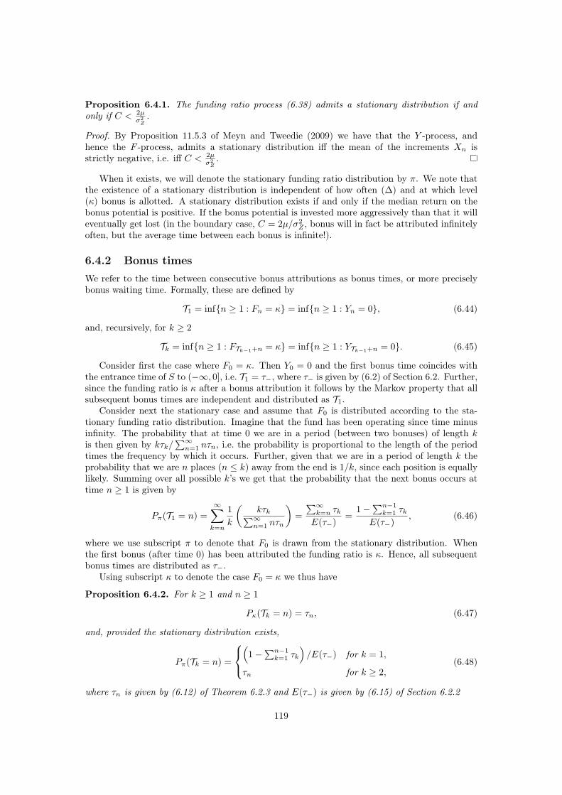
Proposition 6.4.1. The funding ratio process (6.38) admits a stationary distribution if andonly if C < 2µ

σ2Z.

Proof. By Proposition 11.5.3 of Meyn and Tweedie (2009) we have that the Y -process, andhence the F -process, admits a stationary distribution iff the mean of the increments Xn isstrictly negative, i.e. iff C < 2µ

σ2Z

.

When it exists, we will denote the stationary funding ratio distribution by π. We note thatthe existence of a stationary distribution is independent of how often (∆) and at which level(κ) bonus is allotted. A stationary distribution exists if and only if the median return on thebonus potential is positive. If the bonus potential is invested more aggressively than that it willeventually get lost (in the boundary case, C = 2µ/σ2

Z , bonus will in fact be attributed infinitelyoften, but the average time between each bonus is infinite!).

6.4.2 Bonus timesWe refer to the time between consecutive bonus attributions as bonus times, or more preciselybonus waiting time. Formally, these are defined by

T1 = infn ≥ 1 : Fn = κ = infn ≥ 1 : Yn = 0, (6.44)

and, recursively, for k ≥ 2

Tk = infn ≥ 1 : FTk−1+n = κ = infn ≥ 1 : YTk−1+n = 0. (6.45)

Consider first the case where F0 = κ. Then Y0 = 0 and the first bonus time coincides withthe entrance time of S to (−∞, 0], i.e. T1 = τ−, where τ− is given by (6.2) of Section 6.2. Further,since the funding ratio is κ after a bonus attribution it follows by the Markov property that allsubsequent bonus times are independent and distributed as T1.

Consider next the stationary case and assume that F0 is distributed according to the sta-tionary funding ratio distribution. Imagine that the fund has been operating since time minusinfinity. The probability that at time 0 we are in a period (between two bonuses) of length kis then given by kτk/

∑∞n=1 nτn, i.e. the probability is proportional to the length of the period

times the frequency by which it occurs. Further, given that we are in a period of length k theprobability that we are n places (n ≤ k) away from the end is 1/k, since each position is equallylikely. Summing over all possible k’s we get that the probability that the next bonus occurs attime n ≥ 1 is given by

Pπ(T1 = n) =∞∑

k=n

1

k

(kτk∑∞

n=1 nτn

)=

∑∞k=n τkE(τ−)

=1−

∑n−1k=1 τk

E(τ−), (6.46)

where we use subscript π to denote that F0 is drawn from the stationary distribution. Whenthe first bonus (after time 0) has been attributed the funding ratio is κ. Hence, all subsequentbonus times are distributed as τ−.

Using subscript κ to denote the case F0 = κ we thus have

Proposition 6.4.2. For k ≥ 1 and n ≥ 1

Pκ(Tk = n) = τn, (6.47)

and, provided the stationary distribution exists,

Pπ(Tk = n) =

(1−

∑n−1k=1 τk

)/E(τ−) for k = 1,

τn for k ≥ 2,(6.48)

where τn is given by (6.12) of Theorem 6.2.3 and E(τ−) is given by (6.15) of Section 6.2.2

119

Note that in stationarity the probability of receiving bonus in any given year is

Pπ(rB1 > 0) = Pπ(Y1 = 0) = Pπ(T1 = 1) =

1

E(τ−). (6.49)

This relationship is also known as Kac’s theorem.In the stationary case the drift of S is negative and it is not hard to show that the criterion

of Theorem 6.2.6 is satisfied for all n. Hence, the time between bonuses has factorial momentsof all orders and these can be calculated by (6.20) of Theorem 6.2.6.5

6.4.3 Number of bonusesThe number of bonuses in a given period can be calculated from the bonus time distribution.Let Rk = T1 + . . . + Tk denote the time of the k’th bonus, also known as the renewal epochs.For F0 = κ and F0 ∼ π the distribution of Rk can be calculated by the recursion

P∗(R1 = n) = P∗(T1 = n), (6.50)

P∗(Rk = n) =

n−1∑j=k−1

P∗(Rk−1 = j)τn−j . (6.51)

where P∗(T1 = n) is given by Proposition 6.4.2 (and ∗ is either κ or π).Let Nn denote the number of bonuses from time 1 to time n. We have

P∗(Nn ≤ k) = P∗(Rk+1 > n) = 1−n∑

j=k+1

P∗(Rk+1 = j), (6.52)

where ∗ is either κ or π.

6.4.4 Bonus percentageThe bonus percentage distribution can be derived from the (descending) ladder height distribu-tion of the random walk. For F0 = κ the events (T1 = n) and (τ− = n) are identical and on thisevent the bonus percentage given by (6.33) becomes

rBn =κ− 1

κ

(e−Sn − 1

). (6.53)

The mean bonus percentage given the time of bonus can then be calculated by use of Theo-rem 6.2.8.

Proposition 6.4.3. For n ≥ 1

Eκ

(rBn∣∣T1 = n

)=κ− 1

κ

[E(e−Sn

∣∣τ− = n)− 1], (6.54)

where

E(e−Sn

∣∣τ− = n)= − 1

τn

∑σ∈Dn

sgn(σ)

dσ

n∏k=1

(E(e−Sk ;Sk ≤ 0

))σk (6.55)

with

E(e−Sk ;Sk ≤ 0

)= ekCµ∆Φ

(√k∆

µ+ 12Cσ

2Z

σZ

). (6.56)

Further, for n ≥ 1 and provided the stationary distribution exists

Eπ

(rBn∣∣T1 = n

)=

1

Pπ(T1 = n)

∞∑k=0

Eκ

(rBn+k

∣∣T1 = n+ k) τk+n

E(τ−). (6.57)

5In fact, it can be shown that Y is so-called geometrically ergodic which implies exponential moments of thereturn time to 0, i.e. the time between bonuses.

120

Proof. Formula (6.54) follows directly from (6.53). Theorem 6.2.8 identifies the conditionaldistribution of Sn given τ− = n as a linear combination of conditional normal tail measures.Since the normal distribution has exponential moments of all orders we conclude (6.55) bydominated convergence. Expression (6.56) follows from (6.42) by standard calculations.

For the stationary case we consider a fund which has been run since time minus infinity. Letλ denote time since bonus was last attributed,

λ = infn ≥ 0 : F−n = κ = infn ≥ 0 : Y−n = 0. (6.58)

By the argument of Section 6.4.2 leading to (6.46) and the Markov property we have

Pπ (T1 = n, λ = k) =1

n+ k

(n+ k)τk+n

E(τ−)=

τk+n

E(τ−), (6.59)

Eπ

(rBn∣∣T1 = n, λ = k

)= Eκ

(rBn+k

∣∣T1 = n+ k). (6.60)

By summing over all possible values of λ we obtain

Eπ

(rBn∣∣T1 = n

)=

1

Pπ(T1 = n)Eπ

(rBn ; T1 = n

)=

1

Pπ(T1 = n)

∞∑k=0

Eπ

(rBn ; T1 = n, λ = k

)=

1

Pπ(T1 = n)

∞∑k=0

Eπ

(rBn∣∣T1 = n, λ = k

)Pπ (T1 = n, λ = k) . (6.61)

Finally, inserting (6.59) and (6.60) in (6.61) yields (6.57).

Higher order polynomial moments of rB can be expressed in terms of exponential momentsof Sn by expanding (6.53). It is straightforward to extend Proposition 6.4.3 to cover this casealso.

6.4.5 Funding ratioWe consider at last the funding ratio of the fund given that no bonus has yet been attributed.For F0 = κ the events (T1 > n) and (τ− > n) are identical and on this event

Fn = (κ− 1)e−Sn + 1. (6.62)

Polynomial funding ratio moments can be derived by use of Theorem 6.2.9. For the mean fundingratio we have the following result.

Proposition 6.4.4. For n ≥ 1

Eκ

(Fn

∣∣T1 > n)= (κ− 1)E

(e−Sn

∣∣τ− > n)+ 1, (6.63)

where

E(e−Sn |τ− > n) =1

P (τ− > n)

∑σ∈Dn

1

dσ

n∏k=1

(E(e−Sk ;Sk > 0)

)σk (6.64)

with

E(e−Sk ;Sk > 0

)= ekCµ∆Φ

(−√k∆

µ+ 12Cσ

2Z

σZ

). (6.65)

Further, for n ≥ 1 and provided the stationary distribution exists

Eπ

(Fn

∣∣T1 > n)=

1

Pπ(T1 > n)

∞∑k=0

Eκ

(Fn+k

∣∣T1 > n+ k)Pπ(T1 = n+ k + 1), (6.66)

121

Proof. We will only prove (6.66). With λ as in (6.58) and by use of (6.59) we have

Pπ(T1 > n, λ = k) =

∞∑i=n+1

Pπ(T1 = i, λ = k) =

∞∑i=n+1

τi+k

E(τ−)= Pπ(T1 = n+ k + 1), (6.67)

and, by the Markov property,

Eπ

(Fn

∣∣T1 > n, λ = k)= Eκ

(Fn+k

∣∣T1 > n+ k). (6.68)

Then

Eπ

(Fn

∣∣T1 > n)=

1

Pπ(T1 > n)Eπ (Fn; T1 > n)

=1

Pπ(T1 > n)

∞∑k=0

Eπ (Fn; T1 > n, λ = k)

=1

Pπ(T1 > n)

∞∑k=0

Eπ

(Fn

∣∣T1 > n, λ = k)Pπ(T1 > n, λ = k). (6.69)

By inserting (6.67) and (6.68) into (6.69) we obtain (6.66).

6.5 Numerical applicationIn the following we calculate key statistics for the pension fund model of Section 6.3, and weillustrate how these statistics are influenced by the bonus threshold (κ) and the investmentstrategy (C). Based on the results of Section 6.4 we calculate the bonus time distribution,bonus time moments, the number of bonuses, the expected bonus and the expected fundingratio given no bonus. Statistics are calculated for a fund at the bonus threshold and for a fundin stationarity.

In Section 6.5.2 we consider a pension saver paying one monetary unit to the pension fundand receiving 40 years later his terminal pension benefit as a lump sum. Closed form expressionsfor the pension benefit mean and variance are derived for a fund at the bonus threshold at thetime of the contribution. Further, we present in Proposition 6.5.1 an exact simulation algorithmwhich allows the calculation of the pension benefit mean and variance in stationarity. This isused to find the investment strategy optimizing the expected payout in stationarity for givenbonus threshold, i.e. the expected payout for the average saver.

Exact samples from the stationary distribution can also be obtained by the algorithm of Ensorand Glynn (2000). Their algorithm uses exponential tilting and requires exponential moments ofthe innovation distribution to generate independent, identically distributed samples. In contrast,our algorithm generates partly dependent, identically distributed samples with no distributionalassumptions.

We assume throughout that bonus is attributed (possibly) once a year (∆ = 1), and we usethe following capital market parameters r = 3%, µ = 4%, and σZ = 15%.

6.5.1 CharacterizationAs a base case example we choose C = 1.5 and κ = 1.5. Thus when the fund is at the bonusthreshold 2/3 of contributions are guaranteed the risk-free rate r. For contributions committed tothe fund at lower funding ratios, i.e. in periods between bonuses, a larger fraction is guaranteed.

Note that since C is larger than one the bonus potential is leveraged, i.e. the amount investedin stocks is larger than the bonus potential. At the bonus threshold the fraction of total assetsinvested in stocks is given by (1−(1/κ))C. For a base case fund at the bonus threshold a fractionof 1/2 of total assets are invested in stocks.

122

Stationarity

Only investment strategies which give rise to a stationary funding ratio process are consideredviable options for a collective pension fund. Otherwise the funding ratio will (essentially) con-verge to one implying that all assets are invested in the risk-free asset only or, equivalently, thatall contributions are fully guaranteed. Since one of the purposes of entering a collective fund isto get access to the capital market in a cost-effective way, the latter situation defies the purposeof an investment collective.6

Proposition 6.4.1 provides an upper bound on the investment strategy, C, for a stationarydistribution to exist. The bound depends on the capital market parameters only, and neither onthe threshold (κ) nor the frequency of possible bonus attributions (∆). For the capital marketparameters stated above the fund admits a stationary distribution if and only if C is at most3.56. Hence, with C = 1.5 the base case fund is stationary.

For higher values of σZ and/or smaller values of µ the upper bound is appreciably smaller.For the higher, but not unrealistic, volatility of σZ = 20% and with the same risk-premium ofµ = 4% the upper bound on C is 2. For a base case fund at the threshold the bonus potentialconstitutes one third of total assets. In this case, a bound of 2 implies that the fund can invest atmost two thirds of its assets in stocks. Thus, the stationarity requirement can impose materialconstraints on the investment strategy. Figure 6.1 illustrates the upper bound on C for differentmarket parameter sets.

0.00 0.02 0.04 0.06 0.08 0.10

05

1015

20

µ

C

Figure 6.1: Upper bound on the fraction of the bonus potential invested in risky assets (C) fora stationary funding ratio process to exist. The bound is shown as a function of expected excessreturn of the risky asset (µ) for selected values of volatility (σZ). From highest to lowest thebounds correspond to σZ = 10%, 12.5%, 15%, 17.5% and 20%. The dot indicates the base casevalues of (µ,C) = (4%, 1.5).

6The other main purpose of a collective fund is the ability to provide lifelong benefit streams through “di-versification” of the individual member’s time of death. However, in the current paper we do not consider thisaspect.

123

Bonus times

The first bonus time, T1, measures the time of the first bonus after time zero. For a fund initiallyat the bonus threshold the distribution of T1 can be identified as the distribution of τ−, i.e. theentrance time to (−∞, 0] of the associated random walk. For a fund in stationarity, however, ittypically takes longer before the first bonus is attributed since the funding ratio at time zero isoften below the bonus threshold. Once the first bonus is attributed, the waiting time betweenall subsequent bonuses is distributed as τ− regardless of the funding ratio at time zero.

It turns out, perhaps somewhat surprising, that for a fund starting out either at the bonusthreshold or in stationary the distribution of T1 depends only on the investment strategy, andnot on the bonus threshold.7 The top left plot of Figure 6.2 shows the distribution of T1 inthese two cases as given by Proposition 6.4.2. For a base case fund at the bonus threshold theprobability of bonus first year is over fifty percent, while the same probability in stationarity isonly about twenty percent. The large difference between these values implies that in stationaritythe fund is typically “between bonuses”.

The probability of bonus first year as a function of the investment strategy is shown inthe bottom left plot of Figure 6.2. For a fund at the bonus threshold, the probability is overfifty percent for all considered investment strategies albeit decreasing in C. The stationaryprobability on the other hand tends to zero as C approaches the upper bound for stationarityof 3.56. Recall that the stationarity probability also has the interpretation as the long-termaverage, i.e. the frequency with which bonus will be attributed over long horizons (regardless ofthe initial funding status).

Moments of the time between bonuses can be calculated by Theorem 6.2.6. The mean andstandard deviation for various values of C are shown in Table 6.2; as mentioned above thedistribution and hence the moments depend only on the investment strategy. In the base casethe mean is five years, but with a standard deviation of almost fourteen years. Thus there isconsiderable variability in the length of the periods between bonuses. For larger values of C themean and, in particular, the standard deviation increase. A fund with C = 3 is still stationarybut there will be decades, and even centuries, with no bonus. However, by Proposition 6.4.1 wehave that the funding ratio admits a stationary distribution iff the median return on the bonuspotential is positive (for a base case fund that is C<3.56). In other words, the stationarityrequirement imposes a median time between bonuses8 of 1. We conclude that the distributionof the waiting times between bonuses is heavily right skewed.

C 1 1.5 2 2.5 3E(τ−) 4.12 5.02 6.49 9.35 17.39SD(τ−) 9.87 13.73 20.93 37.55 98.60

Table 6.2: The mean and standard deviation of time between bonuses for different investmentstrategies C. In all cases the median is 1.

Number of bonuses

The number of bonuses from time 1 to time n is denoted Nn. The distribution of Nn can becalculated from the distributions of T1 and τ− as described in Section 6.4.3. For a fund startingout either at the bonus threshold or in stationary the distribution of Nn depends only on theinvestment strategy, and not on the bonus threshold.

The top right plot of Figure 6.2 shows the distribution of N40 for a base case fund. For abase case fund starting out at the bonus threshold the distribution of N40 is unimodal and the

7However, for a fund starting out at a given funding ratio (below the bonus threshold) the distribution of T1does of course depend on the bonus threshold also.

8Defined as minn ∈ N :∑ni=1 τi ≥ 0.5

124

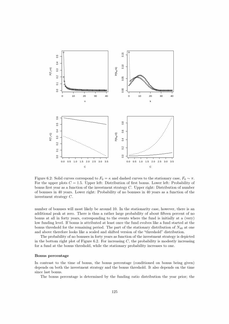
0 10 20 30 40

0.0

0.1

0.2

0.3

0.4

0.5

n

P(T

1=n)

0 10 20 30 40

0.00

0.05

0.10

0.15

k

P(N

40=k

)

0.0 0.5 1.0 1.5 2.0 2.5 3.0 3.5

0.0

0.1

0.2

0.3

0.4

0.5

0.6

C

P(T

1=1)

0.0 0.5 1.0 1.5 2.0 2.5 3.0 3.5

0.0

0.2

0.4

0.6

0.8

C

P(N

40=0

)

Figure 6.2: Solid curves correspond to F0 = κ and dashed curves to the stationary case, F0 ∼ π.For the upper plots C = 1.5. Upper left: Distribution of first bonus. Lower left: Probability ofbonus first year as a function of the investment strategy C. Upper right: Distribution of numberof bonuses in 40 years. Lower right: Probability of no bonuses in 40 years as a function of theinvestment strategy C.

number of bonuses will most likely be around 10. In the stationarity case, however, there is anadditional peak at zero. There is thus a rather large probability of about fifteen percent of nobonus at all in forty years, corresponding to the events where the fund is initially at a (very)low funding level. If bonus is attributed at least once the fund evolves like a fund started at thebonus threshold for the remaining period. The part of the stationary distribution of N40 at oneand above therefore looks like a scaled and shifted version of the “threshold” distribution.

The probability of no bonuses in forty years as function of the investment strategy is depictedin the bottom right plot of Figure 6.2. For increasing C, the probability is modestly increasingfor a fund at the bonus threshold, while the stationary probability increases to one.

Bonus percentage

In contrast to the time of bonus, the bonus percentage (conditioned on bonus being given)depends on both the investment strategy and the bonus threshold. It also depends on the timesince last bonus.

The bonus percentage is determined by the funding ratio distribution the year prior; the

125

higher the funding ratio the higher the conditional expected bonus.9 If a fund starting at thebonus threshold does not give bonus in the first year the funding ratio will be strictly below thebonus threshold. This implies that bonus in the second year (if given) is smaller than bonusin the first year (if given). This argument is hard to continue formally, but it seems at leastintuitively reasonable that the expected bonus will be decreasing in the time since last bonus.

The bonus percentage conditioned on the value of T1 can be calculated by Proposition 6.4.3.It is shown in the top left plot of Figure 6.3 for the base case fund. We see that the conditionalexpected bonus quickly drops by one to two percentage points depending on how the fund isstarted, and then levels off to just below 5.5%.

The middle left plot of Figure 6.3 shows the expected value of the first bonus,

E(rBT1) =

∞∑n=1

E(rBn |T1 = n)P (T1 = n), (6.70)

for the base case fund. The expected bonus (when given) is increasing in C, both in stationarityand for a fund starting at the bonus threshold. In stationarity, however, the frequency withwhich bonus is attributed decreases with C, cf. lower left plot of Figure 6.2. The average bonusin stationarity is therefore a trade-off between many, small bonuses and few, large bonuses. Theaverage bonus in stationarity,

Eπ(rB) = Eπ(r

B1 |T1 = 1)Pπ(T1 = 1), (6.71)

is shown in the lower left plot of Figure 6.3. It is seen that the long-term average bonus ismaximized for C just below 2.

It follows from Proposition 6.4.3 that the average bonus for funds with the same C butdifferent bonus thresholds are linearly related. Specifically, the average bonus in stationarity isrelated by

E(C,κ2)π (rB) =

κ2 − 1

κ2

κ1κ1 − 1

E(C,κ1)π (rB). (6.72)

This implies that plots for different thresholds are scaled versions of each other. In particular,the average bonus in stationarity is maximized for the same C. It also follows that the averagebonus for a fund with κ = 3 is twice as high as the average bonus for a fund with κ = 1.5 (basecase value). Of course, the guaranteed part to which bonus is applied is correspondingly smaller.

Funding ratio

The pension payoff depends on the funding ratio when contributions are committed, the bonusesup to the time of payout, and the funding ratio at payout. Thus to evaluate the payoff we needto consider both the funding ratio at the time money enters the fund, and the funding ratio atthe time money leaves the fund.

The expected funding ratio as a function of the time since last bonus can be calculated byProposition 6.4.4. This is shown for the base case fund in the upper right plot of Figure 6.3.The expected funding ratio is decreasing in the time since last bonus. Intuitively, this seemsreasonable since absence of bonus indicates that the fund is experiencing poor investment results.It is perhaps surprising, however, that the (expected) funding ratio seems to level off, at around120%. Thus beyond a certain point the funding ratio does not deteriorate any further. Limitingdistributions of Markov chains conditioned on non-absorption (or in our case no bonus) are knownas Yaglom limits. We conjecture that the fund possesses a Yaglom limit both in stationarityand when started at the threshold, i.e. that the funding ratio distribution conditioned on nobonus converges to a non-degenerate distribution. However, establishing existence, let aloneidentifying, Yaglom limits is non-trivial and a formal study is outside the scope of this paper.

9This in fact is not obvious, since we condition on bonus being given. It can nevertheless be shown as aconsequence of stochastic ordering and log-concavity of the normal distribution.

126

0 10 20 30 40

0.05

00.

055

0.06

00.

065

0.07

00.

075

n

E[r nB |

T1=

n]

0 10 20 30 40

1.0

1.1

1.2

1.3

1.4

n

E[F n

| T

1>

n]

0.0 0.5 1.0 1.5 2.0 2.5 3.0 3.5

0.00

0.05

0.10

0.15

C

E(r T

1

B)

0.0 0.5 1.0 1.5 2.0 2.5 3.0 3.5

1.0

1.1

1.2

1.3

1.4

1.5

C

E[F 4

0 | T

1>

40]

0.0 0.5 1.0 1.5 2.0 2.5 3.0 3.5

0.00

20.

004

0.00

60.

008

0.01

00.

012

0.01

4

C

E π(rB )

0.0 0.5 1.0 1.5 2.0 2.5 3.0 3.5

1.0

1.1

1.2

1.3

1.4

1.5

C

E π[F

]

Figure 6.3: Solid curves correspond to F0 = κ and dashed curves to the stationary case, F0 ∼π. Bonus threshold κ = 1.5 in all plots. Upper left: Conditional expected bonus percentage(C = 1.5). Middle left: Expected first bonus. Lower left: Expected bonus in stationarity. Upperright: Conditional expected funding ratio given no bonus (C = 1.5). Middle right: Conditionalexpected funding ratio given no bonus in 40 years. Lower right: Expected funding ratio instationarity.

The interested reader is referred to the specialist literature on quasi-stationarity, e.g. Tweedie(1974); Jacka and Roberts (1995); Lasserre and Pearce (2001).10

10The partial result that the funding ratio given no bonus does not converge to one can be obtained without too

127

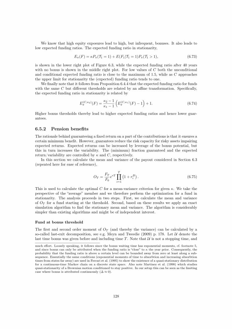
We know that high equity exposures lead to high, but infrequent, bonuses. It also leads tolow expected funding ratios. The expected funding ratio in stationarity,

Eπ(F ) = κPπ(T1 = 1) + E(F1|T1 = 1)Pπ(T1 > 1), (6.73)

is shown in the lower right plot of Figure 6.3, while the expected funding ratio after 40 yearswith no bonus is shown in the middle right plot. For low values of C both the unconditionaland conditional expected funding ratio is close to the maximum of 1.5, while as C approachesthe upper limit for stationarity the (expected) funding ratio tends to one.

We finally note that it follows from Proposition 6.4.4 that the expected funding ratio for fundswith the same C but different thresholds are related by an affine transformation. Specifically,the expected funding ratio in stationarity is related by

E(C,κ2)π (F ) =

κ2 − 1

κ1 − 1

(E(C,κ1)

π (F )− 1)+ 1. (6.74)

Higher bonus thresholds thereby lead to higher expected funding ratios and hence lower guar-antees.

6.5.2 Pension benefitsThe rationale behind guaranteeing a fixed return on a part of the contributions is that it ensures acertain minimum benefit. However, guarantees reduce the risk capacity for risky assets impairingexpected returns. Expected returns can be increased by leverage of the bonus potential, butthis in turn increases the variability. The (minimum) fraction guaranteed and the expectedreturn/variability are controlled by κ and C, respectively.

In this section we calculate the mean and variance of the payout considered in Section 6.3(repeated here for ease of reference),

OT =FT

F0erT

T∏i=1

(1 + rBi

). (6.75)

This is used to calculate the optimal C for a mean-variance criterion for given κ. We take theperspective of the “average” member and we therefore perform the optimization for a fund instationarity. The analysis proceeds in two steps. First, we calculate the mean and varianceof OT for a fund starting at the threshold. Second, based on these results we apply an exactsimulation algorithm to find the stationary mean and variance. The algorithm is considerablysimpler than existing algorithms and might be of independent interest.

Fund at bonus threshold

The first and second order moment of OT (and thereby the variance) can be calculated by aso-called last-exit decomposition, see e.g. Meyn and Tweedie (2009) p. 178. Let U denote thelast time bonus was given before and including time T . Note that U is not a stopping time, and

much effort. Loosely speaking, it follows since the bonus waiting time has exponential moments, cf. footnote 5,and since bonus can only be attributed when the funding ratio is “close” to κ the year prior. Consequently, theprobability that the funding ratio is above a certain level can be bounded away from zero at least along a sub-sequence. Essentially the same conditions (exponential moments of time to absorbtion and increasing absorbtiontimes from states far away) are used in Ferrari et al. (1995) to show the existence of a quasi-stationary distributionfor a continuous-time Markov chain on a discrete state space. Also note Martinez et al. (1998) which studiesquasi-stationarity of a Brownian motion conditioned to stay positive. In our setup this can be seen as the limitingcase where bonus is attributed continuously (∆ ≈ 0).

128

that the decomposition is not a consequence of the Markov property. We have

Eκ(OT ) =Eκ(OT ; T1 > T ) +

T∑j=1

Eκ(OT ;U = j)

=erT

κeκ(T ) +

erT

κ

T∑j=1

∑σ∈Dj

cσ

j∏i=1

(τiEκ

(1 + rBi

∣∣T1 = i))σi

eκ(T − j), (6.76)

where for σ ∈ Dj and n = 0, . . . , T ,

cσ =(∑j

i=1 σi)!∏ji=1 σi!

, eκ(n) = Pκ(T1 > n)Eκ(Fn

∣∣T1 > n). (6.77)

The expression for Eκ(OT ;U = j) follows by considering the different ways bonus can be at-tributed such that the last bonus falls at time j. The different patterns of time between bonusesare given by the permutations in Dj . For each pattern the probability of it occurring and theassociated expected bonus can be calculated by the Markov property, and this has to be multi-plied by the number of ways the “bonus waiting periods” can be arranged, given by cσ. Finally,we multiply by the expected funding ratio given that no bonuses are given for the remainingperiod, given by eκ(T − j). The quantities appearing in expressions (6.76) and (6.77) can becalculated by Propositions 6.4.2–6.4.4.

For the second order moment we similarly find

Eκ(O2T ) =Eκ(O

2T ; T1 > T ) +

T∑j=1

Eκ(O2T ;U = j)

=e2rT

κ2sκ(T ) +

e2rT

κ2

T∑j=1

∑σ∈Dj

cσ

j∏i=1

(τiEκ

((1 + rBi

)2 ∣∣T1 = i))σi

sκ(T − j), (6.78)

where cσ is given by (6.77) and for n = 0, . . . , T ,

sκ(n) = Pκ(T1 > n)Eκ(F2n

∣∣T1 > n). (6.79)

In order to calculate sκ(k) note that on the event (T1 > n)

F 2n =

((κ− 1)e−Sn + 1

)2= (κ− 1)2e−2Sn + 2(κ− 1)e−Sn + 1. (6.80)

Hence, we need to calculate conditional expectations of e−Sn and e−2Sn . The first of these is givenby (6.64) of Proposition 6.4.4. The latter can be calculated by the same formula upon replacingthe term E(e−Sn ;Sn > 0) with E(e−2Sn ;Sn > 0). To evaluate (6.78) we also need to calculatethe second order moment of the bonus percentage. Similarly to F 2

n the term (1 + rBi )2 can beexpanded and expressed in terms of e−Si and e−2Si . The appropriate conditional expectationsof the latter quantities can be calculated by formula (6.55) of Proposition 6.4.3. We omit thedetails.

Fund in stationarity

We are interested in calculating the stationary mean and variance of OT . From Proposi-tions 6.4.2–6.4.4 we know the time and size of first bonus, moments of the initial funding ratioand moments of the terminal funding ratio conditioned on no bonuses. Unfortunately, we needthe joint distribution of these quantities and this is not available in an analytically tractableform. Instead we will apply a simulation algorithm based on samples from the joint stationarydistribution of (F0, T1, rBT1

, FT1∧T ). The idea is to split the period in two, the time up to first

129

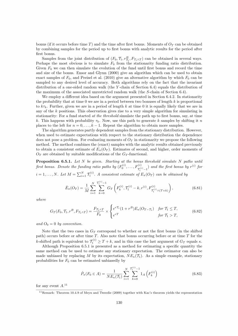
bonus (if it occurs before time T ) and the time after first bonus. Moments of OT can be obtainedby combining samples for the period up to first bonus with analytic results for the period afterfirst bonus.

Samples from the joint distribution of (F0, T1, rBT1, FT1∧T ) can be obtained in several ways.

Perhaps the most obvious is to simulate F0 from the stationarity funding ratio distribution.Given F0 we can then simulate the evolution of the fund until first bonus and record the timeand size of the bonus. Ensor and Glynn (2000) give an algorithm which can be used to obtainexact samples of F0, and Preisel et al. (2010) give an alternative algorithm by which F0 can besampled to any desired level of accuracy. Both algorithms rely on the fact that the invariantdistribution of a one-sided random walk (the Y -chain of Section 6.4) equals the distribution ofthe maximum of the associated unrestricted random walk (the S-chain of Section 6.4).

We employ a different idea based on the argument presented in Section 6.4.2. In stationaritythe probability that at time 0 we are in a period between two bonuses of length k is proportionalto kτk. Further, given we are in a period of length k at time 0 it is equally likely that we are inany of the k positions. This observation gives rise to a very simple algorithm for simulating instationarity: For a fund started at the threshold simulate the path up to first bonus, say, at timek. This happens with probability τk. Now, use this path to generate k samples by shifting it nplaces to the left for n = 0, . . . , k − 1. Repeat the algorithm to obtain more samples.

The algorithm generates partly dependent samples from the stationary distribution. However,when used to estimate expectations with respect to the stationary distribution the dependencedoes not pose a problem. For evaluating moments of OT in stationarity we propose the followingmethod. The method combines the (exact) samples with the analytic results obtained previouslyto obtain a consistent estimate of Eπ(OT ). Estimates of second, and higher, order moments ofOT are obtained by suitable modifications of the GT -functional.

Proposition 6.5.1. Let N be given. Starting at the bonus threshold simulate N paths untilfirst bonus. Denote the funding ratio paths by (F

(i)0 , . . . , F

(i)

T (i)1 −1

) and the first bonus by r(i) for

i = 1, . . . , N . Let M =∑N

i=1 T(i)1 . A consistent estimate of Eπ(OT ) can be obtained by

Eπ(OT ) =1

M

N∑i=1

T (i)1 −1∑k=0

GT

(F

(i)k , T (i)

1 − k, r(i), F(i)

T (i)1 ∧(T+k)

), (6.81)

where

GT (F0, T1, rB , FT1∧T ) =FT1∧T

F0×

erT1(1 + rB)Eκ(OT−T1) for T1 ≤ T,

erT for T1 > T,(6.82)

and O0 = 0 by convention.

Note that the two cases in GT correspond to whether or not the first bonus (in the shiftedpath) occurs before or after time T . Also note that bonus occurring before or at time T for thek-shifted path is equivalent to T (i)

1 ≥ T + k, and in this case the last argument of GT equals κ.Although Proposition 6.5.1 is presented as a method for estimating a specific quantity the

same method can be used to estimate any stationary expectation. The estimator can also bemade unbiased by replacing M by its expectation, NEκ(T1). As a simple example, stationaryprobabilities for F0 can be estimated unbiasedly by

Pπ(F0 ∈ A) =1

NEκ(T1)

N∑i=1

T (i)1 −1∑k=0

1A

(F

(i)k

)(6.83)

for any event A.11

11Remark: Theorem 10.4.9 of Meyn and Tweedie (2009) together with Kac’s theorem yields the representation

130

Mean-variance analysis

We are now in a position to do a mean-variance analysis of the payout OT with respect tothe strategy parameters κ and C. We assume a horizon of T = 40 years. This correspondsapproximately to the average time between when contributions are made and benefits are paidout in a pension fund with life-long memberships.

We first consider a fund starting at the bonus threshold. Table 6.3 states the mean, theminimum (guarantee) and the standard deviation of the payout for different sets of (κ,C). Inall cases the mean equals 6. For the smallest value of κ the payout is guaranteed to be at least2.656. To reach an expected payout of 6 the bonus potential has to be leveraged substantially,and this in turn leads to a large standard deviation. As κ increases the guarantee decreases andan expected payout of 6 can be achieved by investing the bonus potential less aggressively. Thisreduces the standard deviation at the price of a larger downside risk (lower guarantee). In thelimit as κ tends to infinity there is no guarantee and an expected payout of 6 can be achievedwith a standard deviation of 2.17 by investing 37 percent of total assets in stocks.12

κ 1.25 1.5 2 3 5 10C 2.705 1.259 0.782 0.570 0.468 0.413mean 6 6 6 6 6 6guarantee 2.656 2.213 1.660 1.107 0.664 0.332std. dev. 3.662 2.603 2.356 2.256 2.214 2.191

Table 6.3: Mean, guarantee and standard deviation of O40 for a pension fund starting at thebonus threshold. All sets of strategies (κ,C) imply a mean payout of 6.

Consider next a pension fund which has fixed the bonus threshold at κ. This implies thatat least 1/κ of contributions is guaranteed the risk free rate. The value of the threshold mightbe stipulated by regulation to ensure a certain minimum pension, or it might be decided by theboard of the pension fund based on social economic considerations. In either case, the fund needsto determine an investment strategy C. One (common) way to balance the desire for a highpayout against unwanted variability is by use of a mean-variance optimization criterion. Beinga collective pension fund we want to optimize the fund for the benefit of the average member,i.e. in stationarity. Hence, we consider the following stationary mean-variance problem for fixedκ

supC

Eπ(OT )− γVarπ(OT ) . (6.84)

In Figure 6.4 the optimization problem with γ = 0.07468 and T = 40 is illustrated for κ = 1.5and κ = 3. The value of γ is chosen such that 60 percent in stocks is optimal for a mean-variance investor with no guarantee and a constant proportion of total assets in stocks. Wesee from Figure 6.4 that neither the mean nor the standard deviation is monotone in C. Theexpected payout is decreasing for C sufficiently large because very aggressive strategies lead tolow funding ratios in stationarity. The fund with low guarantees (κ = 3) has an optimal C ofabout 80 percent, while the fund with high guarantees (κ = 1.5) has an optimal C of about 150percent. The equity exposure, at the threshold, as a fraction of total assets is about 50 percentfor both cases.

The mean-variance criterion is normally applied in situations where more risk (higher C)leads to higher expected return and higher variability. It might be argued that the mean-variance criterion is considered out of necessity to avoid degenerate solutions in these situations.

result Pπ(F0 ∈ A) = Eκ(∑T1−1k=0 1A(Fk))/Eκ(T1). This result can also be obtained from (6.83) by taking

expectation on both sides. Conversely, it follows from the representation that the right-hand side of (6.83) is anunbiased estimator of Pπ(F0 ∈ A) as claimed.

12For the optimal mean-variance investment strategy see Korn (1997a) and Zhou and Li (2000).

131

In stationarity, however, the expected payout as a function of C is unimodal. We might thereforealternatively define the optimal investment strategy C∗ as the one maximizing the expectedpayout in stationarity. The optimal investment strategy C∗ thus defined is illustrated in Table 6.4and Figure 6.4 upper left for different values of κ. We see that C∗ is considerably higher than theone obtained from the mean-variance criterion (for given κ). However, the associated standarddeviation is also considerably higher implying than the payout will typically deviate substantiallyfrom its expectation.

κ 1 1.25 1.5 2 3 5 10C∗ N/A 2.143 2.313 2.473 2.700 2.850 2.951maximal mean 3.320 4.923 6.886 11.73 23.66 48.50 93.61std. dev. 0 2.213 6.649 26.13 151.5 826.9 3540

Table 6.4: The optimal investment strategy, C∗, maximizing the expectation of O40 in station-arity for different values of κ. The corresponding mean and standard deviation of O40 are alsoshown.

0.0 0.5 1.0 1.5 2.0 2.5 3.0 3.5

510

1520

C

Expe

cted

bene

fit at

retire

ment

0.0 0.5 1.0 1.5 2.0 2.5 3.0 3.5

02

46

8

C

Std.

dev

iation

of b

enef

it at r

etire

ment

0.0 0.5 1.0 1.5 2.0 2.5 3.0 3.5

010

020

030

0

C

Std.

dev

iation

of b

enef

it at r

etire

ment

0.0 0.5 1.0 1.5 2.0 2.5 3.0 3.5

01

23

45

6

C

mean

−var

Figure 6.4: Stationary mean and standard deviation of O40 as a function of the investmentstrategy C. Solid curves correspond to κ = 1.5 and dotted curves to κ = 3. Upper left:Expected pension payout. Upper right and lower left: Standard deviation of the pension payout(note the different scales). Lower right: Illustration of the mean-variance optimization problem(6.84).

132

6.6 Appendix (proofs)

6.6.1 Entrance times and partitionsProof of Theorem 6.2.3. Rearranging (6.5) we get for 0 ≤ s < 1

1− exp

( ∞∑n=1

(−1)pnnsn

)=

∞∑n=1

τnsn. (6.85)

From Theorem 6.2.2 we get that

exp

( ∞∑n=1

(−1)pnnsn

)= 1 +

∞∑m=1

∑σ∈Dm

sm

σ1!σ2! · · ·σm!

m∏n=1

((−1)

pnn

)σn

= 1 +

∞∑m=1

∑σ∈Dm

sgn(σ)

dσsm

m∏n=1

pσnn . (6.86)

Insert this in (6.85) to obtain

−∞∑

m=1

∑σ∈Dm

sgn(σ)

dσsm

m∏n=1

pσnn =

∞∑n=1

τnsn. (6.87)

Finally, by inspection of the left and right hand side of the above equality we obtain (6.12).

Proof of Theorem 6.2.4. We need to prove two identities∑σ∈Dn

kσkdσ

= 1, (6.88)

and ∑σ∈Dn

1

dσ= 1. (6.89)

We first note that (6.89) follows from (6.88) by summing over k. Using that∑n

k=1 kσk = nfor σ ∈ Dn we get

n =n∑

k=1

∑σ∈Dn

kσkdσ

=∑σ∈Dn

∑nk=1 kσkdσ

=∑σ∈Dn

n

dσ, (6.90)

and dividing through by n yields (6.89).We next prove (6.88) by induction in n. For n = 1 the relation is trivially satisfied. Assume

that (6.88) holds for n− 1 and all 1 ≤ k ≤ n− 1; then (6.89) also holds for n− 1 as just shown.To prove that (6.88) holds for n and 1 ≤ k ≤ n there are three cases to consider:

For k = n the only term in the sum different from zero occurs for σ = (0, . . . , 0, 1), and hence∑σ∈Dn

nσn∏ni=1 σi!i

σi=

n

1!n= 1. (6.91)

For 1 < k < n we use that there is a one-to-one mapping between permutations in Dn withσk > 0 and permutations in Dn−1 with πk−1 > 0 defined by π = (σ1, . . . , σk−2, σk−1 + 1, σk −

133

1, σk+1, . . . , σk−1). Noting that σk > 0 with k < n implies σn = 0 we have∑σ∈Dn

kσk∏ni=1 σi!i

σi

=∑

σ∈Dn:σk>0

kσk∏n−1i=1 σi!i

σi

=∑

π∈Dn−1:πk−1>0

k(πk + 1)∏n−1i=1 πi!i

πi

πk−1!(k − 1)πk−1πk!kπk

(πk−1 − 1)!(k − 1)πk−1−1(πk + 1)!kπk+1

=∑

π∈Dn−1:πk−1>0

(k − 1)πk−1∏n−1i=1 πi!i

πi

= 1, (6.92)

where the last equality follows by the induction hypothesis.For k = 1 the mapping π = (σ1 − 1, σ2, . . . , σn−1) is one-to-one between permutations in Dn

with σ1 > 0 and all permutations in Dn−1. We then have∑σ∈Dn

σ1∏ni=1 σi!i

σi=

∑π∈Dn−1

π1 + 1∏n−1i=1 πi!i

πi

π1!

(π1 + 1)!=

∑π∈Dn−1

1∏n−1i=1 πi!i

πi

= 1, (6.93)

where the last equality follows from (6.89) which holds for n−1 by the induction hypothesis.

6.6.2 Entrance time momentsProof of Theorem 6.2.5. Let G1 = H ′ and define recursively

Gn = H ′Gn−1 +G′n−1 (n ≥ 2). (6.94)

We first establish the relation

τ (n) = −eHGn (n ≥ 1). (6.95)

Clearly, the relation holds for n = 1. Assuming (6.95) holds for n− 1 we have by (6.94)

τ (n) =(−eHGn−1

)′= −eH

(H ′Gn−1 +G′

n−1

)= −eHGn, (6.96)

and hence (6.95) holds for all n by induction.Having established (6.95) we now need to prove

Gn =∑σ∈Dn

cσHσ (n ≥ 1). (6.97)

As before we will prove this by induction. For n = 1 the equation reads G1 = H ′ which is trueby definition. Assume (6.97) holds for n− 1. By (6.94) and the induction hypothesis we have

Gn =∑

σ∈Dn−1

cσH′Hσ +

∑σ∈Dn−1

cσ(Hσ)′, (6.98)

134

where for σ = (σ1, . . . , σn−1) ∈ Dn−1

(Hσ)′ = σ1H

σ1−11 Hσ2

2

n−1∏i=2

Hσii +Hσ1

1

(n−1∏i=2

Hσii

)′

= . . .

=n−1∑k=1

σkHσk−1k Hk+1

∏i =k

Hσii . (6.99)

Thus

Gn =∑

σ∈Dn−1

cσH′Hσ +

∑σ∈Dn−1

n−1∑k=1

cσσkHσk−1k Hk+1

∏i =k

Hσii . (6.100)

Let σ∗ = (σ∗1 , . . . , σ

∗n) ∈ Dn be fixed, but arbitrary. We will identify the terms in (6.100) which

contain the factor Hσ∗and show that the coefficients add up to cσ∗ . There are three cases (note

that in the first two cases the condition implies that σ∗n = 0):

1. σ∗1 > 0: Then H ′Hσ = Hσ∗

with σ = (σ∗1 − 1, σ∗

2 , . . . , σ∗n−1) ∈ Dn−1. The first sum in

(6.100) contains a term with this factor and coefficient cσ.

2. σ∗j > 0 for some 2 ≤ j ≤ n−1: ThenHσk−1

k Hk+1

∏i =kH

σii = Hσ∗

with σ = (σ∗1 , . . . , σ

∗j−2, σ

∗j−1+

1, σ∗j − 1, σ∗

j+1, . . . , σ∗n−1) ∈ Dn−1 and k = j − 1. The second sum in (6.100) contains a

term with this factor and coefficient cσ(σ∗j−1 + 1).

3. σ∗n > 0: In this case σ∗ = (0, . . . , 0, 1) and hence Hσ∗

= Hn = Hσk−1k Hk+1

∏i =kH

σii for

σ = (0, . . . , 0, 1) ∈ Dn−1 and k = n−1. This term is included in the second sum of (6.100)with coefficient cσ.

Hence, for each positive component of σ∗ there exists a term in (6.100) containing the factorHσ∗

. Conversely, every term in (6.100) corresponds to a σ∗ ∈ Dn and is of the form covered inone of the three cases above. Hence, we have

Gn =∑

σ∗∈Dn

Hσ∗ ∑1≤j≤n:σ∗

j>0

(σ∗j−1 + 1)cσ(j) (6.101)

where σ(j) = (σ∗1 , . . . , σ

∗j−2, σ

∗j−1 + 1, σ∗

j − 1, σ∗j+1, . . . , σ

∗n−1) ∈ Dn−1 and we, for notational

convenience, define σ∗0 ≡ 0. Using (6.10) we can write the inner sum in (6.101) as∑

1≤j≤n:σ∗j>0

(σ∗j−1 + 1)cσ(j)

=∑

1≤j≤n:σ∗j>0

(σ∗j−1 + 1)

(n− 1)!∏n−1i=1 σ

(j)i !(i!)σ

(j)i

=1∏n

i=1 σ∗i !(i!)

σ∗i

∑1≤j≤n:σ∗

j>0

(σ∗j−1 + 1)(n− 1)!

∏ni=1 σ

∗i !(i!)

σ∗i∏n−1

i=1 σ(j)i !(i!)σ

(j)i

=1∏n

i=1 σ∗i !(i!)

σ∗i

∑1≤j≤n:σ∗

j>0

(σ∗j−1 + 1)(n− 1)!

σ∗j j!

(σ∗j−1 + 1)(j − 1)!

=1∏n

i=1 σ∗i !(i!)

σ∗i(n− 1)!

∑1≤j≤n:σ∗

j>0

σ∗j j

=n!∏n

i=1 σ∗i !(i!)

σ∗i

= cσ∗ , (6.102)

135

where the penultimate equality uses that∑

1≤j≤n:σ∗j>0 σ

∗j j = n since σ∗ ∈ Dn. This shows that

(6.97) holds and we are finished.

Before proving Theorem 6.2.6 we need to state the following two lemmas:

Lemma 6.6.1. For n ≥ 1, (a1, . . . , an) ∈ Cn and b ∈ C

∑σ∈Dn

n∏i=1

(ai −

bi

i

)σi 1

σi!=∑σ∈Dn

n∏i=1

aσii

σi!− b

∑σ∈Dn−1

n−1∏i=1

aσii

σi!, (6.103)

where the last sum is 1 by definition for n = 1.

Proof. We first note that the left-hand side of (6.103) can be written

∑σ∈Dn

n∏i=1

aσii

σi!− b

∑σ∈Dn

σ1aσ1−11

σ1!

n∏i=2

aσii

σi!+ . . . , (6.104)

where . . . denotes higher order terms of b. Since there is only a contribution to the first orderterm if σ1 > 0, and since σ ∈ Dn with σ1 > 0 if and only if (σ1 − 1, σ2, . . . , σn−1) ∈ Dn−1, wehave that the first order term is given by

b∑

σ∈Dn:σ1>0

σ1aσ1−11

σ1!

n∏i=2

aσii

σi!= b

∑σ∈Dn−1

n−1∏i=1

aσii

σi!. (6.105)

Hence we are finished if we show that all higher order terms in (6.104) vanish.For m ≥ 2, the m’th order terms are of the form

n∏i=1

aηi

i

(−bi

i

)νi 1

(ηi + νi)!

(ηi + νiνi

)=

sgn(ν)

dνbm

n∏i=1

aηi

i

ηi!, (6.106)

where ν ∈ Dm and η ∈ Dn−m, with the convention that νj = 0 for j > m and, similarly, ηj = 0for j > n − m (for m = n, ηj = 0 for all j). The higher order terms in (6.104) can then bewritten

n∑m=2

bm∑

η∈Dn−m

n∏i=1

aηi

i

ηi!

∑ν∈Dm

sgn(ν)

dν= 0, (6.107)

since the inner sum is zero for m ≥ 2 by equation (6.13).

We also need the following combination of Kronecker’s lemma, see e.g. Theorem 2.5.5 ofDurrett (2010), and Frobenius’ theorem, see e.g. Chapter 7 of Duren (2012).

Lemma 6.6.2. If∑∞

k=1 ak converges to a finite limit then

f(s) = (1− s)∞∑k=1

skkak (6.108)

converges for |s| < 1 and f(s) → 0 as s→ 1−.

Proof. Let bk = k and xk = kak. Then bk ↑ ∞ and, by assumption,∑∞

k=1 xk/bk =∑∞

k=1 akconverges. By Kronecker’s lemma this implies that

1

bn

n∑k=1

xk =1

n

n∑k=1

kak → 0 as n→ ∞. (6.109)

136

Next, let a0 = 0 and ck = kak − (k − 1)ak−1 for k ≥ 1. Summation by parts yields

f(s) = (1− s)∞∑k=1

skkak =∞∑k=1

sk(kak − (k − 1)ak−1) =∞∑k=1

skck, (6.110)

where the series∑∞

k=1 ck is Cesàro summable to zero by (6.109), i.e. the average of the par-tial sums,

∑km=1 cm = kak, converges to zero. By Frobenius’ theorem we conclude that f(s)

converges for |s| < 1 and f(s) → 0 as s→ 1−.

With those two lemmas available we are now ready to prove Theorem 6.2.6.

Proof of Theorem 6.2.6. By Theorem 6.2.5 we have for |s| < 1

τ (n)(s) = −eH(s)∑σ∈Dn

cσHσ(s), (6.111)

where H(s) = −∑∞

k=1sk

k P (Sk ≤ 0) and

Hσ(s) =

n∏i=1

(−

∞∑k=i

(k)iksk−iP (Sk ≤ 0)

)σi

. (6.112)

Using that log(1− s) = −∑∞

k=1 sk/k, and hence (i− 1)!/(1− s)i =

∑∞k=i s

k−i(k)i/k, we get

eH(s) = exp

( ∞∑k=1

sk

k(1− P (Sk ≤ 0))−

∞∑k=1

sk

k

)

= exp

( ∞∑k=1

sk

kP (Sk > 0)

)(1− s), (6.113)

and

cσHσ(s) = n!n∏

i=1

( ∞∑k=i

(k)iksk−i(1− P (Sk ≤ 0))−

∞∑k=i

(k)iksk−i

)σi

1

σi!(i!)σi

= n!n∏

i=1

( ∞∑k=i

(k)iksk−iP (Sk > 0)− (i− 1)!

(1− s)i

)σi

1

σi!(i!)σi

= n!

n∏i=1

(ai −

bi

i

)σi 1

σi!, (6.114)

where ai =∑∞

k=i(k)ik sk−iP (Sk > 0)/i! and b = 1/(1− s). By Lemma 6.6.1 we then have

∑σ∈Dn

cσHσ(s)/n! =∑σ∈Dn

n∏i=1

aσii

σi!− b

∑σ∈Dn−1

n−1∏i=1

aσii

σi!. (6.115)

Theorem 6.2.5 in combination with (6.113) and (6.115) yields

τ (n)(s) = exp

( ∞∑k=1

sk

kP (Sk > 0)

) ∑σ∈Dn−1

ncσ

n−1∏i=1

( ∞∑k=i

(k)iksk−iP (Sk > 0)

)σi

− exp

( ∞∑k=1

sk

kP (Sk > 0)

) ∑σ∈Dn

(1− s)cσ

n∏i=1

( ∞∑k=i

(k)iksk−iP (Sk > 0)

)σi

. (6.116)

137

By assumption∑∞

k=1 kn−2P (Sk > 0) <∞, and by dominated convergence, all series of order at

most n− 2 thereby converge to finite limits as s tends to 1−. In combination with Lemma 6.6.2we also have

lims→1−

(1− s)∞∑

k=n

(k)nk

sk−nP (Sk > 0) = 0, (6.117)

and we conclude

E((τ−)n) = lims→1−

τ (n)(s) = exp

( ∞∑k=1

1

kP (Sk > 0)

)n!

∑σ∈Dn−1

n−1∏i=1

(hii!

)σi 1

σi!<∞. (6.118)

6.6.3 Conditional characteristic functionsProof of Theorem 6.2.8. Define the (partial) characteristic functions

γn(ζ) = E(eiζSn ; τ− = n

), (6.119)

in terms of which χ can be written as

χ(s, ζ) =∞∑

n=1

snγn(ζ). (6.120)

Rearranging (6.26) we get

1− exp

(−

∞∑n=1

sn

ngn

)=

∞∑n=1

snγn(ζ), (6.121)

where we have defined gn = E(eiζSn ;Sn ≤ 0

). From Theorem 6.2.2 we get that

exp

( ∞∑n=1

(−1)gnnsn

)= 1 +

∞∑m=1

∑σ∈Dm

sm

σ1!σ2! · · ·σm!

m∏n=1

((−1)

gnn

)σn

= 1 +∞∑

m=1

∑σ∈Dm

sgn(σ)

dσsm

m∏n=1

gσnn . (6.122)

Insert this in (6.121) to obtain

−∞∑

m=1

∑σ∈Dm

sgn(σ)

dσsm

m∏n=1

gσnn =

∞∑n=1

snγn(ζ). (6.123)

By inspection of the left and right hand side of the equality above we obtain

γn(ζ) = −∑σ∈Dn

sgn(σ)

dσ

n∏k=1

(E(eiζSk ;Sk ≤ 0

))σk. (6.124)

Finally, divide by τn to obtain (6.27).

Proof of Theorem 6.2.9. For fixed ζ and n we have the following first-entrance decomposition

E(eiζSn) =n∑

k=1

E(eiζSn ; τ− = k) + E(eiζSn ; τ− > n)

=n∑

k=1

E(eiζSk ; τ− = k)E(eiζSn−k) + E(eiζSn ; τ− > n), (6.125)

138

where the second equality follows from the Markov property and the random walk structure.For ease of notation we let ek = E(eiζSk). In this notation, the decomposition above can bewritten

E(eiζSn ; τ− > n) = en −n∑

k=1

E(eiζSk ; τ− = k)en−k. (6.126)

Multiplying both sides of (6.126) by e1 yields the relation

E(eiζSn ; τ− > n)e1 = en+1 −n∑

k=1

E(eiζSk ; τ− = k)en+1−k

= E(eiζSn+1 ; τ− > n+ 1) + E(eiζSn+1 ; τ− = n+ 1), (6.127)

where we have used that for all k, eke1 = ek+1.We are now ready to prove (6.28) by induction in n. Since the events (τ− > 1) and (S1 > 0)

are identical equation (6.28) holds for n = 1. Next, assume that (6.28) holds for n. Lete+k = E(eiζSk ;Sk > 0) and note that E(eiζSk ;Sk ≤ 0) = ek − e+k . From Theorem 6.2.8 we have

E(eiζSn+1 ; τ− = n+ 1) = −∑

σ∈Dn+1

n+1∏k=1

(e+k − ek

k

)σk1

σk!. (6.128)

Using that ek = ek1 we get from (6.127), the induction hypothesis and (6.128) that

E(eiζSn+1 ; τ− > n+ 1) = e1∑σ∈Dn

n∏k=1

(e+kk

)σk1

σk!+

∑σ∈Dn+1

n+1∏k=1

(e+k − ek1

k

)σk1

σk!

=∑

σ∈Dn+1

n+1∏k=1

(e+kk

)σk1

σk!, (6.129)

where the second equality uses Lemma 6.6.1 with ak = e+k /k and b = e1. This shows that (6.28)holds for n+ 1 and we are finished.

139

140

Bibliography

E. S. Andersen. On the fluctuations of sums of random variables II. Mathematica Scandinavica2, pages 195–223, 1954.

S. Asmussen. Applied Probability and Queues, second edition. Springer-Verlag, New York, 2003.

S. Basak and G. Chabakauri. Dynamic mean-variance asset allocation. The Review of FinancialStudies 23(8), pages 2970–3016, 2010.

T. Björk and A. Murgoci. A general theory of Markovian time inconsistent stochastic controlproblems. Working paper, Stockholm School of Economics, 2009.

T. Björk, A. Murgoci, and X. Zhou. Mean variance portfolio optimization with state dependentrisk aversion. Mathematical Finance, pages 1–24, 2012.

E. Briys and F. de Varenne. On the risk of insurance liabilities: debunking some common pitfalls.Journal of Risk and Insurance 64(4), pages 673–694, 1997.

K. Bruhn and M. Steffensen. Household consumption, investment and life insurance. InsuranceMathematics and Economics 48(3), pages 315–325, 2011.

M. M. Carhart. On persistence in mutual fund performance. Journal of Finance 52, pages 57–82,1997.

J. C. Cox and C.-F. Huang. Optimal consumption and portfolio policies when asset prices followa diffusion process. Journal of Economic Theory 49(1), pages 33–83, 1989.

J. C. Cox and C.-F. Huang. A variational problem arising in financial economics. Journal ofMathematical Economics 20(5), pages 465–487, 1991.

J. Cvitanic and I. Karatzas. Convex duality in constrained portfolio optimization. Annals ofApplied Probability 2(4), pages 767–818, 1992.

J. Cvitanic, J. P. Lehoczky, and I. Karatzas. Optimal portfolio and consumption decisions for a’small investor’ on a finite horizon. SIAM Journal on Control and Optimization 25(6), pages1557–1586, 1987.

T. M. Døskeland and H. A. Nordahl. Optimal pension insurance design. Journal of Banking &Finance 32(3), pages 382–392, 2008.

D. Duffie and T. Zariphopoulou. Optimal investment with undiversifiable income risk. Mathe-matical Finance 3(2), pages 135–148, 1993.

D. Duffie, W. Fleming, H. Soner, and T. Zariphopoulou. Hedging in incomplete markets withHARA utility. Journal of Economic Dynamics and Control 21(4–5), pages 753–782, 1997.

P. Duren. Invitation to Classical Analysis. American Mathematical Society, 2012.

141

R. Durrett. Probability: Theory and Examples, fourth edition. Cambridge University Press,Cambridge, 2010.

P. H. Dybvig and H. Liu. Lifetime consumption and investment: Retirement and constrainedborrowing. Journal of Economic Theory 145(3), pages 885–907, 2010.

I. Ekeland and A. Lazrak. Being serious about non-commitment: subgame perfect equilibriumin continuous time. Priprint, University of British Columbia, 2006.

I. Ekeland and T. A. Pirvu. Investment and consumption without commitment. Mathematicsand Financial Economics 2(1), pages 57–86, 2008.

N. El-Karoui and M. Jeanblanc. Optimization of consumption with labor income. Finance andStochastic 2(4), pages 409–440, 1998.

N. El-Karoui and I. Karatzas. The optimal stopping problem for a general American put-option.In Mathematics Finance (M. Davis, D. Duffie, W. Fleming. and S. Shreve, eds.) IMA Vol.65, 77–88. Springer-Verlag, New York, 1995.

N. El-Karoui, M. Jeanblanc, and V. Lacoste. Optimal portfolio management with Americancapital guarantee. Journal of Economic Dynamics and Control 29(3), pages 449–468, 2005.

K. B. Ensor and P. W. Glynn. Simulating the maximum of a random walk. Journal of StatisticalPlanning and Inference 85, pages 127–135, 2000.

E. F. Fama and K. R. French. Luck versus skill in the cross-section of mutual fund returns.Journal of Finance 5, pages 1915–1947, 2010.

E. Farhia and S. Panageas. Saving and investing for early retirement: A theoretical analysis.Journal of Financial Economics 83(1), pages 87–121, 2007.

W. Feller. An Introduction to Probability Theory and Its Applications, Vol. II, second edition.Wiley, New York, 1971.

P. A. Ferrari, H. Kesten, S. Martinez, and P. Picco. Existence of quasi-stationary distributions.A renewal dynamical approach. Annals of Probability 23(2), pages 501–521, 1995.

W. H. Fleming and R. W. Richel. Deterministic and Stochastic Optimal Control. Springer-Verlag, New York, Berlin, Heidelberg, 1975.

H. U. Gerber and W. W. Shiu. Investing for retirement: Optimal capital growth and dynamicasset allocation. North American Actuarial Journal 4, pages 42–58, 2000.

J. Gil-Bazo and P. Ruiz-Verdú. The relation between price and performance in the mutual fundindustry. Journal of Finance 64(5), pages 2153–2183, 2009.

A. Grosen and P. L. Jørgensen. Fair valuation of life insurance liabilities: The impact of in-terest rate guarantees, surrender options, and bonus policies. Insurance: Mathematics andEconomics 26(1), pages 37–57, 2000.

M. Guillén, S. F. Jarner, J. P. Nielsen, and A. M. Pérez-Marín. Risk-adjusted impact of admin-istration costs in the distribution of terminal wealth for passive investment, mutual and hedgefunds. Working Paper, 2013.

G. H. Hardy and S. Ramanujan. Asymtotic formulæ in combinatory analysis. Proceedings of theLondon Mathematical Society 2.1, pages 75–115, 1918.

H. He and H. F. Pagès. Labor income, borrowing constraints, and equilibrium asset prices.Economic Theory 3(4), pages 663–696, 1993.

142

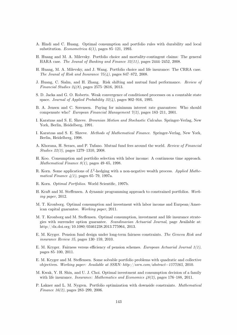
A. Hindi and C. Huang. Optimal consumption and portfolio rules with durability and localsubstitution. Econometrica 6(1), pages 85–121, 1993.

H. Huang and M. A. Milevsky. Portfolio choice and mortality-contingent claims: The generalHARA case. The Jounal of Banking and Finance 32(11), pages 2444–2452, 2008.

H. Huang, M. A. Milevsky, and J. Wang. Portfolio choice and life insurance: The CRRA case.The Jounal of Risk and Insurance 75(4), pages 847–872, 2008.

J. Huang, C. Sialm, and H. Zhang. Risk shifting and mutual fund performance. Review ofFinancial Studies 24(8), pages 2575–2616, 2013.

S. D. Jacka and G. O. Roberts. Weak convergence of conditioned processes on a countable statespace. Journal of Applied Probability 32(4), pages 902–916, 1995.

B. A. Jensen and C. Sørensen. Paying for minimum interest rate guarantees: Who shouldcompensate who? European Financial Management 7(2), pages 183–211, 2001.

I. Karatzas and S. E. Shreve. Brownian Motion and Stochastic Calculus. Springer-Verlag, NewYork, Berlin, Heidelberg, 1991.

I. Karatzas and S. E. Shreve. Methods of Mathematical Finance. Springer-Verlag, New York,Berlin, Heidelberg, 1998.

A. Khorana, H. Seraes, and P. Tufano. Mutual fund fees around the world. Review of FinancialStudies 22(3), pages 1279–1310, 2008.

H. Koo. Consumption and portfolio selection with labor income: A continuous time approach.Mathematical Finance 8(1), pages 49–65, 1998.

R. Korn. Some applications of L2-hedging with a non-negative wealth process. Applied Mathe-matical Finance 4(1), pages 65–79, 1997a.

R. Korn. Optimal Portfolios. World Scientific, 1997b.

H. Kraft and M. Steffensen. A dynamic programming approach to constrained portfolios. Work-ing paper, 2012.

M. T. Kronborg. Optimal consumption and investment with labor income and Eurpean/Amer-ican capital guarantee. Working paper, 2011.

M. T. Kronborg and M. Steffensen. Optimal consumption, investment and life insurance strate-gies with surrender option guarantee. Scandinavian Actuarial Journal, page Available at:http://dx.doi.org/10.1080/03461238.2013.775964, 2013.

E. M. Kryger. Pension fund design under long-term fairness constraints. The Geneva Risk andinsurance Review 35, pages 130–159, 2010.

E. M. Kryger. Fairness versus efficiency of pension schemes. European Actuarial Journal 1(1),pages 85–100, 2011.

E. M. Kryger and M. Steffensen. Some solvable portfolio problems with quadratic and collectiveobjectives. Working paper: Available at SSRN: http://ssrn.com/abstract=1577265, 2010.

M. Kwak, Y. H. Shin, and U. J. Choi. Optimal investment and consumption decision of a familywith life insurance. Insurance: Mathematics and Economics 48(2), pages 176–188, 2011.

P. Lakner and L. M. Nygren. Portfolio optimization with downside constraints. MathematicalFinance 16(2), pages 283–299, 2006.

143

J. B. Lasserre and C. E. M. Pearce. On the existence of a quasistationary measure for a Markovchain. Annals of Probability 29(1), pages 437–446, 2001.

H. Markowitz. Portfolio selection. Journal of Finance 7(1), pages 77–91, 1952.

S. Martinez, P. Picco, and J. S. Martin. Domain of attraction of quasi-stationary distributionsfor the Brownian motion with drift. Advances in Applied Probability 30(2), pages 385–408,1998.

R. Merton. Lifetime portfolio selection under uncertainty: The continuous-time case. Review ofEconomics and Statistics 51(3), pages 247–257, 1969.

R. Merton. Optimum consumption and portfolio rules in a continuous-time model case. Journalof Economic Theory 3, pages 373–413, 1971.

S. P. Meyn and R. L. Tweedie. Markov chains and stochastic stability, 2nd edition. London:Springer-Verlag, 2009.

M. A. Milevsky and V. R. Young. Annuitization and asset allocation. Jounal of economicdynamics and control 31(9), pages 3138–3177, 2007.

C. Munk. Optimal consumption/investment policies with undiversifiable income risk and liquid-ity constraints. Journal of Economic Dynamics and Control 24(9), pages 1315–1343, 2000.

P. H. Nielsen. Utility maximization and risk minimization in life and pension insurance. Finanseand Stochastics 10, pages 75–97, 2006.

P. H. Nielsen and M. Steffensen. Optimal investment and life insurance strategies under minimumand maximum constraints. Insurance Mathematics and Economics 43(1), pages 15–28, 2008.

R. Norberg. A theory of bonus in life insurance. Finance and Stochastics 3, pages 373–390, 1999.

R. Norberg. On bonus and bonus prognoses in life insurance. Scandinavian Actuarial Journal22, pages 126–147, 2001.

J. Palczewski, R. Poulsen, K. R. Schenck-Hoppé, and H. Wang. Dynamic portfoliooptimization with transaction costs and state-dependent drift. Working paper, pagehttp://papers.ssrn.com/sol3/papers.cfm?abstract_id=2346304, 2013.

S. R. Pliska and J. Ye. Optimal life insurance purchase and consumption/investment underuncertain lifetime. Journal of Banking and Finance 31(5), pages 1307–1319, 2007.

M. Preisel, S. F. Jarner, and R. Eliasen. Investing for retirement through a with-profits pensionscheme: a client’s perspective. Scandinavian Actuarial Journal 1, pages 15–35, 2010.

S. Richard. Optimal consumption, portfolio and life insurance rules for an uncertain livedindividual in a continuous time model. Journal of Finance Economics 2(2), pages 187–203,1975.

F. Spitzer. A combinatorial lemma and its application to probability theory. Transactions ofthe American Mathematical Society 82, pages 323–339, 1956.

M. Steffensen. Contigent claims analysis in life and pension insurance. Proceedings 10th AFIRColloquium, pages 587–603, 2000.

M. Steffensen. On Merton’s problem for life insurers. ASTIN Bulletin 34(1), pages 5–25, 2004.

M. Steffensen and H. Kraft. Optimal consumption and insurance: A continuous-time markovchain approach. ASTIN Bulletin 38(1), pages 231–257, 2008.

144

R. Strotz. Myopia and inconsistency in dynamic utility maximization. Review of EconomicStudies 23(3), pages 165–180, 1955.

W. Szpankowski. Average Case Analysis of Algorithms on Sequences. Wiley-Interscience, 2001.

L. Teplá. Optimal investment with minimum performance constraints. Journal of EconomicDynamics and Control 25(10), pages 1629–1645, 2001.

R. L. Tweedie. Quasi-stationary distributions for Markov chains on a general state space. Journalof Applied Probability 11(4), pages 726–741, 1974.

M. E. Yaari. Uncertain lifetime, life insurance and the theory of the consumer. Review ofEconomic Studies 32(2), pages 137–150, 1965.

X. Y. Zhou and D. Li. Continuous-time mean-variance portfolio selection: A stochastic LQframwork. Applied Mathematical Optimization 42(1), pages 19–33, 2000.

145