Advances in NowcastingEconomic Activity

Juan Antolın-Dıaz1 Thomas Drechsel2 Ivan Petrella3

CFE - ERCIMLondon

December 18, 2017

1Fulcrum Asset Management2LSE and Centre for Macroeconomics3Warwick Business School and CEPR

This paper

I This paper contributes to the literature on nowcastingeconomic activity.

I We propose a bayesian dynamic factor model (DFM), whichtakes seriously the features of the data:

1. Low-frequency variation in the mean and variance

2. Heterogeneous responses to common shocks (lead-lags)

3. Outlier observations and fat tails

4. Endogenous modeling of seasonality (not today)

I We evaluate performance of the model and new features in acomprehensive out of sample real-time exercise, payingparticular attention to density forecasts.

I The project builds on our earlier work: Antolin-Diaz, Drechsel,and Petrella (2017 ReStat)

Preview of Results

I The results we show today are for the US

I The real-time nowcasting performance is substantiallyimproved across a variety of metrics (point and density)

I Capturing trends and SV improves nowcasting performancesignificantly

I Heterogeneous dynamics deliver substantial additionalimprovement

I Fat tails successfully capture outlier observations in anautomated way and improve density forecasts of the monthlyvariables

Plan of the talk

1. The Model

I Highlight features of the dataI Lay out how these are formally captured in the DFM

2. Estimation

I Brief overview of data and algorithm

3. Setup of Real-Time Evaluation Exercise

4. Evaluation Results

5. Conclusion

The Model

The ModelSpecification

We start from the familiar specification of a DFM(see, e.g. Giannone, Reichlin, and Small, 2008)

Consider an n-dimensional vector of quarterly and monthlyobservables yt, which follows

∆(yt) = c + λft + ut (1)

(I − Φ(L))ft = εt (2)

(1− ρi(L))ui,t = ηi,t, i = 1, . . . , n (3)

εtiid∼ N(0,Σε) (4)

ηi,tiid∼ N(0, σ2

ηi), i = 1, . . . , n (5)

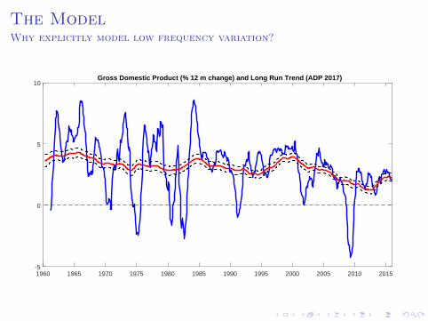
The ModelWhy explicitly model low frequency variation?

1960 1965 1970 1975 1980 1985 1990 1995 2000 2005 2010 2015-5

0

5

10Gross Domestic Product (% 12 m change) and Long Run Trend (ADP 2017)

The ModelSpecification

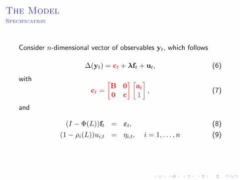
Consider n-dimensional vector of observables yt, which follows

∆(yt) = ct + λft + ut, (6)

with

ct =

[B 00 c

] [at1

], (7)

and

(I − Φ(L))ft = εt, (8)

(1− ρi(L))ui,t = ηi,t, i = 1, . . . , n (9)

The ModelWhy model changes in volatility?

1950 1960 1970 1980 1990 2000 20100

1

2

3

4

5

6

7

8

I SV in the common factor captures both secular (McConnelland Perez-Quiros, 2000) and cyclical (e.g., Jurado et al.,2014) movements in volatility.

The ModelSpecification

Consider n-dimensional vector of observables yt, which follows

∆(yt) = ct + λft + ut, (10)

with

ct =

[B 00 c

] [at1

], (11)

and

(I − Φ(L))ft = σεtεt, (12)

(1− ρi(L))ui,t = σηi,tηi,t, i = 1, . . . , n (13)

where the time-varying parameters will be specified as a randomwalk processes. TVP processes

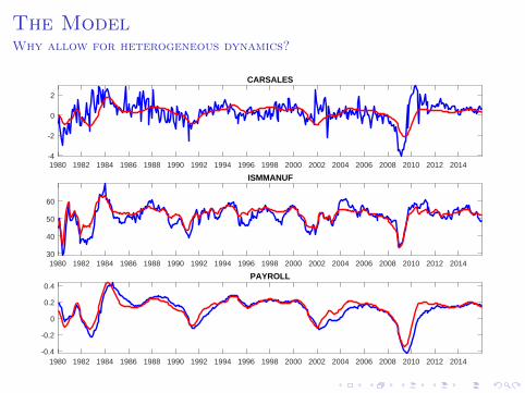
The ModelWhy allow for heterogeneous dynamics?

1980 1982 1984 1986 1988 1990 1992 1994 1996 1998 2000 2002 2004 2006 2008 2010 2012 2014-4

-2

0

2

CARSALES

1980 1982 1984 1986 1988 1990 1992 1994 1996 1998 2000 2002 2004 2006 2008 2010 2012 201430

40

50

60

ISMMANUF

1980 1982 1984 1986 1988 1990 1992 1994 1996 1998 2000 2002 2004 2006 2008 2010 2012 2014-0.4

-0.2

0

0.2

0.4PAYROLL

The ModelSpecification

∆(yt) = ct + Λ(L)ft + ut, (14)

where Λ(L) contains the loadings on the contemporaneous andlagged common factors.

I Camacho and Perez-Quiros (2010) first noticed that surveydata was better aligned with a distributed lag of GDP.

I D’Agostino et al. (2015) show that adding lags improvesperformance in the context of a small model.

The modelWhat do the heterogeneous dynamics achieve?

0 5 10 15 20

Months

0

0.1

0.2

0.3

0.4

0.5

0.6Monotonic

GDPINVESTMENTINDPROCONSUMPTION

0 5 10 15 20

Months

-0.1

0

0.1

0.2

0.3

0.4Reversing

CARSALESPERMITHOUSINGSTARTSNEWHOMESALES

0 5 10 15 20

Months

0

0.1

0.2

0.3

0.4

0.5

0.6Hump Shaped

ISMMANUFCONSCONFPHILLYFEDCHICAGO

Result: There is substantial heterogeneity in the impulseresponses.

The ModelWhy model fat tails?

1960 1965 1970 1975 1980 1985 1990 1995 2000 2005 2010 2015-50

0

50Light Weight Vehicle Sales (% MoM change)

1960 1965 1970 1975 1980 1985 1990 1995 2000 2005 2010 2015-10

-5

0

5

10Real Personal Disposable Income (% 1 m change)

1960 1965 1970 1975 1980 1985 1990 1995 2000 2005 2010 2015-2

-1

0

1

2Civilian Employment (% 1 m change)

The ModelSpecification

∆(yt − ot) = ct + Λ(L)ft + ut, (15)

with ot as well as the innovations to ut following a t-distribution.

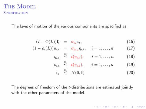
The ModelSpecification

The laws of motion of the various components are specified as

(I − Φ(L))ft = σεtεt, (16)

(1− ρi(L))ui,t = σηi,tηi,t, i = 1, . . . , n (17)

ηi,tiid∼ t(vη,i), i = 1, . . . , n (18)

oi,tiid∼ t(vo,i), i = 1, . . . , n (19)

εtiid∼ N(0, I) (20)

The degrees of freedom of the t-distributions are estimated jointlywith the other parameters of the model.

The modelWhat do the fat tails achieve?

-4 -2 0 2 4-0.1

0

0.1F

acto

r U

pdat

e (p

.p)

INDPRO

-4 -2 0 2 4-0.1

0

0.1

Fac

tor

Upd

ate

(p.p

)

CARSALES

-4 -2 0 2 4-0.1

0

0.1

Fac

tor

Upd

ate

(p.p

)

INCOME

-4 -2 0 2 4-0.1

0

0.1

Fac

tor

Upd

ate

(p.p

)

RETAILSALES

-4 -2 0 2 4-0.1

0

0.1

Fac

tor

Upd

ate

(p.p

)

HOUSINGSTARTS

-4 -2 0 2 4-0.1

0

0.1

Fac

tor

Upd

ate

(p.p

)

NEWHOMESALES

-4 -2 0 2 4-0.1

0

0.1

Fac

tor

Upd

ate

(p.p

)

PAYROLL

-4 -2 0 2 4-0.1

0

0.1

Fac

tor

Upd

ate

(p.p

)

EMPLOYMENT

-4 -2 0 2 4-0.1

0

0.1

Fac

tor

Upd

ate

(p.p

)

CLAIMS

-4 -2 0 2 4-0.1

0

0.1

Fac

tor

Upd

ate

(p.p

)

ISMMANUF

-4 -2 0 2 4-0.1

0

0.1

Fac

tor

Upd

ate

(p.p

)

ISMNONMAN

-4 -2 0 2 4-0.1

0

0.1

Fac

tor

Upd

ate

(p.p

)

CONSCONF

-4 -2 0 2 4

Forecast Error (s.d.)

-0.1

0

0.1

Fac

tor

Upd

ate

(p.p

)

RICHMOND

-4 -2 0 2 4

Forecast Error (s.d.)

-0.1

0

0.1

Fac

tor

Upd

ate

(p.p

)

PHILLYFED

-4 -2 0 2 4

Forecast Error (s.d.)

-0.1

0

0.1

Fac

tor

Upd

ate

(p.p

)

CHICAGO

-4 -2 0 2 4

Forecast Error (s.d.)

-0.1

0

0.1

Fac

tor

Upd

ate

(p.p

)

EMPIRE

News decomposition details

Estimation

EstimationData set for the US case

Frequency

Hard IndicatorsGDP (Chained $) QGDI (Chained $) QConsumption (Chained $, Non Dur. + Serv.) QInvestment (Chained $, Fixed + Cons. Dur.) QAggregate Hours Worked (Total Economy) QIndustrial Production MPayroll Employment (Establishment Survey) MReal Retail Sales Food Services MReal Personal Income less Transfer Payments MNew Orders of Capital Goods MLight Weight Vehicle Sales MReal Exports of Goods MReal Imports of Goods MBuilding Permits MHousing Starts MNew Home Sales MCivilian Employment (Household Survey) MUnemployed MInitial Claims for Unemployment Insurance M

Soft IndicatorsMarkit Manufacturing PMI MISM Manufacturing PMI MISM Non-manufacturing PMI MConference Board: Consumer Confidence MUniversity of Michigan: Consumer Sentiment MRichmond Fed Mfg Survey MPhiladelphia Fed Business Outlook MChicago PMI MNFIB: Small Business Optimism Index MEmpire State Manufacturing Survey M

EstimationAlgorithm (brief overview)

I Model is specified at monthly frequency. Observed growthrates of quarterly variables are related to the unobservedmonthly growth rate using a weighted mean (see Mariano andMurasawa, 2003)

I We use a hierarchical implementation of a Gibbs Sampleralgorithm (Moench, Ng, and Potter, 2013) which iteratesbetween a small DFM on the outlier adjusted data and theunivariate measurement equations. This leads to largecomputational gains due to parallelisation of this step.

I SVs are sampled following Kim et al. (1998).

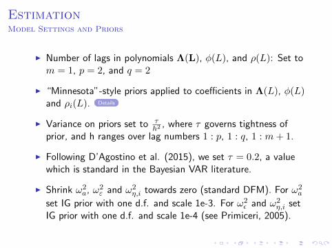
EstimationModel Settings and Priors

I Number of lags in polynomials Λ(L), φ(L), and ρ(L): Set tom = 1, p = 2, and q = 2

I “Minnesota”-style priors applied to coefficients in Λ(L), φ(L)and ρi(L). Details

I Variance on priors set to τh2 , where τ governs tightness of

prior, and h ranges over lag numbers 1 : p, 1 : q, 1 : m+ 1.

I Following D’Agostino et al. (2015), we set τ = 0.2, a valuewhich is standard in the Bayesian VAR literature.

I Shrink ω2a, ω2

ε and ω2η,i towards zero (standard DFM). For ω2

a

set IG prior with one d.f. and scale 1e-3. For ω2ε and ω2

η,i setIG prior with one d.f. and scale 1e-4 (see Primiceri, 2005).

Real-time out of sample evaluation

Real-time out of sample evaluationDetails of data base construction

I We construct a real-time data base for the US and other G7countries: Germany, France, Italy, Canada, UK, and Japan.

I We consider 2744 data vintages since 11 January 2000 to 31December 2015.

I For each vintage, sample start is Jan 1960, appending missingobservations to any series which starts after that date.

I Sources: (1) ALFRED, (2) OECD Original Release andRevisions Data.

I Use appropriate deflators for nominal-only vintages.

I Splice data for series with methodological changes.

I Apply seasonal adjustment in real time for survey data.

Real-time out of sample evaluationImplementation of the exercise

I The model is fully re-estimated every time new data isreleased/revised. The out of sample exercise starts in January2000 and ends in December 2015. For the US, on averagethere is a data release on 15 different dates every month. Thismeans 2744 vintages of data.

I Thanks to efficient implementation of the code, it takes just 2hours to run 8000 iterations of the Gibbs sampler. But thiswould mean 7 months of computations!

I Made feasible by using Amazon Web Services cloudcomputing platform.

Evaluation Results

Evaluation ResultsWhat we show

I In the following slides:

I Model 0 = Baseline DFMI Model 1 = Trend + SVI Model 2 = Trend + SV + heterogeneous dynamicsI Model 3 = Trend + SV + heterogeneous dynamics + fat tails

I We will consider the following metrics

1. RMSE / MAE2. Probability Integral Transform (PITs)3. Log Score4. Continuous Rank Probability Score (CRPS)

I Everything is for US GDP (1st release)

ResultsForecasts vs. actual over time

GDP: Model forecasts vs realizations, day before release

2000 2001 2002 2003 2004 2005 2006 2007 2008 2009 2010 2011 2012 2013 2014 2015

-8

-6

-4

-2

0

2

4

6

Actual Model 0 Model 1

I The addition of the long run trend eliminates the upward biasin GDP forecasts after the crisis...

ResultsForecasts vs. actual over time

GDP: Model forecasts vs realizations, day before release

2000 2001 2002 2003 2004 2005 2006 2007 2008 2009 2010 2011 2012 2013 2014 2015

-8

-6

-4

-2

0

2

4

6

Actual Model 1 Model 2 Model 3

I Heterogeneous dynamics capture recoveries more accurately

ResultsGDP: Root mean squared error (RMSE) across horizons

-180 -150 -120 -90 -60 -30 0

NowcastForecast Backcast

1.4

1.6

1.8

2

2.2

2.4

2.6

Model 0 Model 1 Model 2 Model 3

Note: Results with MAE very similar.

ResultsRoot mean squared error (RMSE), Rolling

2000 2001 2002 2003 2004 2005 2006 2007 2008 2009 2010 2011 2012 2013 2014 20150.4

0.6

0.8

1

1.2

1.4

1.6

1.8

2

2.2

Model 0 Model 1 Model 2 Model 3

Note: Results with MAE very similar.

ResultsLogscore

-180 -150 -120 -90 -60 -30 0

NowcastForecast Backcast

-2.5

-2

-1.5

Model 0 Model 1 Model 2 Model 3

ResultsCRPS

-180 -150 -120 -90 -60 -30 0

NowcastForecast Backcast

0.5

1

1.5

Model 0 Model 1 Model 2 Model 3

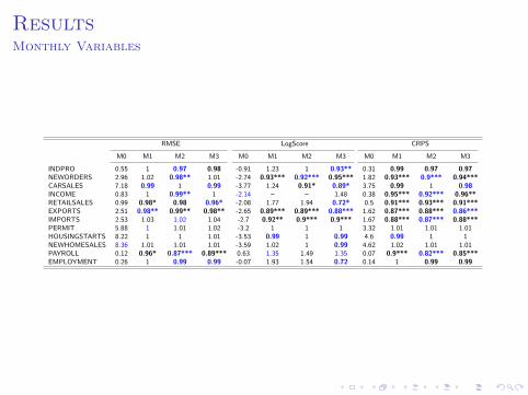
ResultsMonthly Variables

RMSE LogScore CRPS

M0 M1 M2 M3 M0 M1 M2 M3 M0 M1 M2 M3

INDPRO 0.55 1 0.97 0.98 -0.91 1.23 1 0.93** 0.31 0.99 0.97 0.97NEWORDERS 2.96 1.02 0.98** 1.01 -2.74 0.93*** 0.92*** 0.95*** 1.82 0.93*** 0.9*** 0.94***CARSALES 7.18 0.99 1 0.99 -3.77 1.24 0.91* 0.89* 3.75 0.99 1 0.98INCOME 0.83 1 0.99** 1 -2.14 – – 1.48 0.38 0.95*** 0.92*** 0.96**RETAILSALES 0.99 0.98* 0.98 0.96* -2.08 1.77 1.94 0.72* 0.5 0.91*** 0.93*** 0.91***EXPORTS 2.51 0.98** 0.99** 0.98** -2.65 0.89*** 0.89*** 0.88*** 1.62 0.87*** 0.88*** 0.86***IMPORTS 2.53 1.03 1.02 1.04 -2.7 0.92** 0.9*** 0.9*** 1.67 0.88*** 0.87*** 0.88***PERMIT 5.88 1 1.01 1.02 -3.2 1 1 1 3.32 1.01 1.01 1.01HOUSINGSTARTS 8.22 1 1 1.01 -3.53 0.99 1 0.99 4.6 0.99 1 1NEWHOMESALES 8.36 1.01 1.01 1.01 -3.59 1.02 1 0.99 4.62 1.02 1.01 1.01PAYROLL 0.12 0.96* 0.87*** 0.89*** 0.63 1.35 1.49 1.35 0.07 0.9*** 0.82*** 0.85***EMPLOYMENT 0.26 1 0.99 0.99 -0.07 1.93 1.54 0.72 0.14 1 0.99 0.99

Conclusion

Summary and Conclusion

I We propose a bayesian DFM, which incorporates:

1. Low-frequency variation in the mean and variance

2. Heterogeneous responses to common shocks

3. Outlier observations and fat tails

4. Endogenous modeling of seasonality (not today)

I The real-time nowcasting performance is substantiallyimproved across a variety of metrics

I Capturing trends and SV improves nowcasting performancesignificantly

I Heterogeneous dynamics deliver substantial additionalimprovement

I Fat tails improve density forecasts of monthly variables(more to be done)

References

Antolin-Diaz, J., T. Drechsel, and I. Petrella (2017): “Tracking theslowdown in long-run GDP growth,” Review of Economics and Statistics, 99.

Banbura, M. and M. Modugno (2014): “Maximum Likelihood Estimation ofFactor Models on Datasets with Arbitrary Pattern of Missing Data,” Journal ofApplied Econometrics, 29, 133–160.

Camacho, M. and G. Perez-Quiros (2010): “Introducing the euro-sting:Short-term indicator of euro area growth,” Journal of Applied Econometrics, 25,663–694.

D’Agostino, A., D. Giannone, M. Lenza, and M. Modugno (2015):“Nowcasting Business Cycles: A Bayesian Approach to Dynamic HeterogeneousFactor Models,” Tech. rep.

Giannone, D., L. Reichlin, and D. Small (2008): “Nowcasting: The real-timeinformational content of macroeconomic data,” Journal of Monetary Economics,55, 665–676.

Jurado, K., S. C. Ludvigson, and S. Ng (2014): “Measuring Uncertainty,”American Economic Review, Forthcoming.

McConnell, M. M. and G. Perez-Quiros (2000): “Output Fluctuations in theUnited States: What Has Changed since the Early 1980’s?” American EconomicReview, 90, 1464–1476.

Moench, E., S. Ng, and S. Potter (2013): “Dynamic hierarchical factor models,”Review of Economics and Statistics, 95, 1811–1817.

Appendix Slides

The ModelSpecification

The model’s time-varying parameters are specified to followdriftless random walks:

aj,t = aj,t−1 + vaj,t , vaj,tiid∼ N(0, ω2

a,j) j = 1, . . . , r

log σεt = log σεt−1 + vε,t, vε,tiid∼ N(0, ω2

ε)

log σηi,t = log σηi,t−1 + vηi,t , vηi,tiid∼ N(0, ω2

η,i) i = 1, . . . , n

Back to main slides

The modelNews Decompositions

Banbura and Modugno (2014) show in a Gaussian model that theimpact of a new release on the nowcasts can be written as a linearfunction of the news:

E(yk,tk|Ω2)− E(yk,tk|Ω1) = wj (yj,tj − E(yj,tj |Ω))

wj =ΛkE

((ftk − ftk|Ω)(ftj − ftjΩ)

)Λ′j

ΛjE(

(ftj − ftj |Ω)(ftj − ftjΩ))

Λ′j + σ2ηj,tj

Back to main slides

The modelNews Decompositions

We show that with the Student-t distribution the weights are nolonger linear, but depend on the value of the forecast error itself:

E(yk,tk|Ω2)− E(yk,tk|Ω1) = wj(yj,tj) (yj,tj − E(yj,tj |Ω))

wj(yj,tj) =ΛkE

((ftk−ftk|Ω)(ftj−ftjΩ)

)Λ′j

ΛjE(

(ftj−ftj |Ω)(ftj−ftjΩ))

Λ′j+σ2ηj,tj

δj,tj

δj,tj = (((yj,tj − E(yj,tj |Ω))2/σ2ηj,tj + vo,j)/(vo,i + 1)

Large errors are discounted as outlier observations containing lessinformation.

Back to main slides

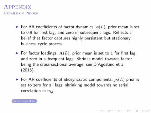
AppendixDetails on Priors

I For AR coefficients of factor dynamics, φ(L), prior mean is setto 0.9 for first lag, and zero in subsequent lags. Reflects abelief that factor captures highly persistent but stationarybusiness cycle process.

I For factor loadings, Λ(L), prior mean is set to 1 for first lag,and zero in subsequent lags. Shrinks model towards factorbeing the cross-sectional average, see D’Agostino et al.(2015).

I For AR coefficients of idiosyncratic components, ρi(L) prior isset to zero for all lags, shrinking model towards no serialcorrelation in ui,t.

Back to main slides