Advances in Type Systems for FunctionalLogic Programming

Proyecto Fin de Máster en Programación y Tecnología Software

Máster en Investigación Informática, Facultad de Informática, Universidad Complutensede Madrid

Author: Enrique Martín MartínDirector: Dr. Francisco Javier López Fraguas

2008-2009

El abajo firmante, matriculado en el Máster en Investigación en Informática de la Facultad de

Informática, autoriza a la Universidad Complutense de Madrid (UCM) a difundir y utilizar con fines

académicos, no comerciales y mencionando expresamente a su autor el presente Trabajo Fin de Máster:

“Advances in Type Systems for Functional Logic Programming”, realizado durante el curso académico

2008-2009 bajo la dirección de D. Francisco Javier López Fraguas en el Departamento de Sistemas In-

formáticos y Computación, y a la Biblioteca de la UCM a depositarlo en el Archivo Institucional E-Prints

Complutense con el objeto de incrementar la difusión, uso e impacto del trabajo en Internet y garantizar

su preservación y acceso a largo plazo.

Fdo: Enrique Martín Martín

SummaryDeclarative languages provide a higher and more abstract level of programming than traditional im-

perative languages. Functional and logic languages are the two most important declarative programming

paradigms, and their combination has been a topic of research in the last two decades. Functional logic

languages have inherited the classical Damas & Milner type system [20] from their functional part, due to

its simplicity and popularity, but this naive approach does not work properly in all cases. It is known that

higher order patterns (HO) in left-hand sides of program rules may produce undesirable effects from the

point of view of types. In particular some expressions can lose their type after a step of computation. In

this work we propose an extension to the classical Damas & Milner type system that fixes this situation.

This problem was first detected in [24], and the proposed solution was forbidding opaque HO patterns.

We propose a more relaxed way of tackle this problem, making a distinction between transparent and

opaque variables. A variable is transparent in a pattern if its type is univocally fixed by the type of the

pattern, and opaque otherwise. We prohibit only the occurrence of opaque variables when they are used

in the right-hand side of the rules. We have developed the type system trying to clarify the behavior

(from the point of view of types) that local definitions have in different implementations of functional

and functional logic languages. This is an issue that varies greatly, and it is not usually well documented

or formalized. Apart from the type system we also present type inference algorithms for expressions

and programs, and provide a prototype of implementation in Prolog that will be soon integrated into the

T OY [45, 69] compiler. We have paid special attention to the formal aspects of the work. Therefore

we have developed detailed proofs of the properties of the type system, in particular the subject reduc-

tion property (expressions keep their type after evaluation), and the soundness and completeness of the

inference algorithms wrt. the type system.

KeywordsType systems, functional logic programming, higher order patterns, opaque patterns, parametric

polymorphism, local definitions, T OY .

ResumenLos lenguajes declarativos proporcionan un nivel de programación más alto y abstracto que los

lenguajes imperativos tradicionales. Los lenguajes funcionales y los lógicos son los dos paradigmas

declarativos más importantes, y su combinación ha sido un tema de investigación en las últimas dos

décadas. Los lenguajes lógico funcionales han heredado el clásico sistema Damas & Milner [20] de su

parte funcional, debido a su simplicidad y popularidad, pero esta aproximación directa no funciona cor-

rectamente en todos los casos. Es conocido que los patrones de orden superior en los lados izquierdos de

las reglas de programa pueden producir efectos no deseados desde el punto de vista de los tipos. En par-

ticular algunas expresiones pueden perder su tipo tras un paso de cómputo. En este trabajo proponemos

una extensión del clásico sistema de tipos Damas & Milner que arregla esta situación. Este problema fue

detectado por primera vez en [24], y la solución propuesta fue prohibir los patrones de orden superior

opacos. Nosotros proponemos una forma más relajada de abordar este problema, haciendo una distinción

entre variables transparentes y opacas. Una variable es transparente en un patrón si su tipo está unívo-

camente determinado por el tipo del patrón, y es opaca en otro caso. Nosotros prohibimos solamente la

aparición de variables opacas cuando son usadas en los lados derechos de las reglas. Hemos desarrollado

el sistema de tipos tratando de clarificar el comportamiento (desde el punto de vista de los tipos) que

las declaraciones locales tienen en diferentes implementaciones de lenguajes funcionales y lógico fun-

cionales. Éste es un aspecto que varía mucho, y usualmente no está bien documentado ni formalizado.

Aparte del sistema de tipos presentamos algoritmos de inferencia de tipos para expresiones y programas,

y proporcionamos un prototipo de implementación en Prolog que será integrado próximamente en el

compilador de T OY [45, 69]. Hemos prestado especial atención a los aspectos formales del trabajo. Por

ello hemos desarrollado demostraciones detalladas de las propiedades del sistema de tipos, en particular

de la propiedad de preservación del tipo o subject reduction (las expresiones mantienen su tipo tras la

evaluación), y la corrección y completitud de los algoritmos de inferencia con respecto al sistema de

tipos.

Palabras claveSistemas de tipos, programación lógico funcional, patrones de orden superior, patrones opacos,

polimorfismo paramétrico, definiciones locales, T OY .

AgradecimientosGracias a Paco por muchas cosas. Primero por haberme enseñado algunas de las asignaturas más

interesantes de la carrera, y por ofrecerme la oportunidad de quedarme en la facultad tras terminar la

carrera (e insistir en ello). Si no fuera por él seguramente ahora mismo no me dedicaría a la investigación,

sino a alguna labor aburrida y estresante en la empresa. Gracias también a él y Juan por haberme ido

introduciendo poco a poco en el mundillo de la investigación en estos dos años, y por todas las reuniones

que hemos tenido (y las que presumiblemente nos quedan). También agradecer al “núcleo duro” del

despacho 220 por crear un ambiente tan bueno, que hace que venir a trabajar sea muchas veces un

placer, especialmente al “Rincón de Nacho”1, oráculo, centro de reuniones y peaje obligatorio para todo

habitante del 220. Y gracias a Sonseca (Toledo) y a toda la gente que allí tengo porque dos días a la

semana puedo olvidarme de todo lo que hago en los otros cinco :-).

Pero sobre todo gracias a Ester y a mi familia, porque sin ellos nada de todo esto que hago tendría

mucho sentido.

1situado en el fondo Norte

Contents

1 Introduction 1

1.1 Type systems . . . . . . . . . . . . . . . . . . . . . . . . . . . . . . . . . . . . . . . . 2

1.1.1 Overview of type systems . . . . . . . . . . . . . . . . . . . . . . . . . . . . . 3

1.2 Functional logic programming . . . . . . . . . . . . . . . . . . . . . . . . . . . . . . . 5

1.3 Motivation . . . . . . . . . . . . . . . . . . . . . . . . . . . . . . . . . . . . . . . . . . 8

1.3.1 Type problems with HO patterns in FLP . . . . . . . . . . . . . . . . . . . . . . 8

1.3.2 Variety of polymorphism in local definitions . . . . . . . . . . . . . . . . . . . 9

1.4 Contributions . . . . . . . . . . . . . . . . . . . . . . . . . . . . . . . . . . . . . . . . 11

2 Preliminaries 13

2.1 Expressions, programs and substitutions . . . . . . . . . . . . . . . . . . . . . . . . . . 13

2.2 Types . . . . . . . . . . . . . . . . . . . . . . . . . . . . . . . . . . . . . . . . . . . . 17

3 Type Derivations 21

3.1 Rules of the type system . . . . . . . . . . . . . . . . . . . . . . . . . . . . . . . . . . 21

3.1.1 Basic typing relation ` . . . . . . . . . . . . . . . . . . . . . . . . . . . . . . . 21

3.1.2 Extended typing relation `• . . . . . . . . . . . . . . . . . . . . . . . . . . . . 26

3.2 Properties of type derivations . . . . . . . . . . . . . . . . . . . . . . . . . . . . . . . . 29

3.3 Subject reduction . . . . . . . . . . . . . . . . . . . . . . . . . . . . . . . . . . . . . . 30

3.3.1 Notion of well-typed program . . . . . . . . . . . . . . . . . . . . . . . . . . . 30

3.3.2 Semantics . . . . . . . . . . . . . . . . . . . . . . . . . . . . . . . . . . . . . . 32

3.3.3 Transformation to simple patterns . . . . . . . . . . . . . . . . . . . . . . . . . 33

3.3.4 Subject reduction property . . . . . . . . . . . . . . . . . . . . . . . . . . . . . 35

4 Type Inference of Expressions 37

4.1 Type inference rules . . . . . . . . . . . . . . . . . . . . . . . . . . . . . . . . . . . . . 37

4.2 Type inference algorithm . . . . . . . . . . . . . . . . . . . . . . . . . . . . . . . . . . 41

4.3 Properties of the type inference . . . . . . . . . . . . . . . . . . . . . . . . . . . . . . . 43

5 Type Inference of Programs 47

5.1 Polymorphic recursion . . . . . . . . . . . . . . . . . . . . . . . . . . . . . . . . . . . 48

5.2 Block inference . . . . . . . . . . . . . . . . . . . . . . . . . . . . . . . . . . . . . . . 49

5.2.1 Properties of block inference . . . . . . . . . . . . . . . . . . . . . . . . . . . . 50

5.3 Stratified inference . . . . . . . . . . . . . . . . . . . . . . . . . . . . . . . . . . . . . 51

6 Implementation 55

6.1 Syntax of the terms. Operators. . . . . . . . . . . . . . . . . . . . . . . . . . . . . . . . 56

6.2 Inference algorithms: infer.pl . . . . . . . . . . . . . . . . . . . . . . . . . . . . . 58

6.3 Strongly connected components algorithm: stronglycc.pl . . . . . . . . . . . . . . 59

6.4 Stratified inference: stratified.pl . . . . . . . . . . . . . . . . . . . . . . . . . . 61

7 Conclusions and Future Work 63

7.1 Contributions of this work . . . . . . . . . . . . . . . . . . . . . . . . . . . . . . . . . 63

7.2 Future work . . . . . . . . . . . . . . . . . . . . . . . . . . . . . . . . . . . . . . . . . 65

Bibliography 67

A Proofs 73

A.1 Previous remarks and easy facts not formally proved . . . . . . . . . . . . . . . . . . . 73

A.2 Proofs of lemmas and theorems . . . . . . . . . . . . . . . . . . . . . . . . . . . . . . . 74

List of Figures

1 Notation . . . . . . . . . . . . . . . . . . . . . . . . . . . . . . . . . . . . . . . . . . XV

1.1 Let expressions in different programming languages . . . . . . . . . . . . . . . . . . 10

2.1 Syntax of expressions . . . . . . . . . . . . . . . . . . . . . . . . . . . . . . . . . . . 14

2.2 Syntax of one-hole contexts and its application . . . . . . . . . . . . . . . . . . . . . 15

2.3 Syntax of the types . . . . . . . . . . . . . . . . . . . . . . . . . . . . . . . . . . . . . 17

3.1 Rules of the type system . . . . . . . . . . . . . . . . . . . . . . . . . . . . . . . . . . 22

3.2 Rule of the extended type system . . . . . . . . . . . . . . . . . . . . . . . . . . . . . 28

3.3 Higher order let-rewriting relation→l . . . . . . . . . . . . . . . . . . . . . . . . . 33

3.4 Transformation rules of let expressions with patterns . . . . . . . . . . . . . . . . . 34

4.1 Type inference rules . . . . . . . . . . . . . . . . . . . . . . . . . . . . . . . . . . . . 38

4.2 Extended type inference rules . . . . . . . . . . . . . . . . . . . . . . . . . . . . . . . 38

4.3 Type inference as an algorithm E . . . . . . . . . . . . . . . . . . . . . . . . . . . . . 42

4.4 Extended type inference as an algorithm E• . . . . . . . . . . . . . . . . . . . . . . . 43

6.1 Syntax of expressions and programs in Prolog . . . . . . . . . . . . . . . . . . . . . 57

6.2 Syntax of types in Prolog . . . . . . . . . . . . . . . . . . . . . . . . . . . . . . . . . 57

6.3 Pseudocode of Tarjan’s algorithm . . . . . . . . . . . . . . . . . . . . . . . . . . . . 60

X,Y, Z . . . Data variable Figure 2.1c Data constructor Figure 2.1f Function Figure 2.1h Data constructor or function symbol Figure 2.1s Data variable, data constructor or function Figure 2.1t Pattern Figure 2.1e Expression Figure 2.1α, β, γ . . . Type variable Figure 2.3τ Simple type Figure 2.3σ Type-scheme Figure 2.3A Set of assumptions Definition 8θ Data substitution Section 2.1π Type substitution Section 2.2` Typing relation Figure 3.1`• Extended typing relation Figure 3.2� Type inference relation Figure 4.1�• Extended type inference relation Figure 4.2E Type inference algorithm Figure 4.3E• Extended type inference algorithm Figure 4.4ΠeA Typing substitutions wrt. ` Definition 16•ΠeA Typing substitutions wrt. `• Definition 16

� Generic instance relation Definition 5Gen(τ,A) Generalization of a type Definition 11�var Variant relation Definition 7P Program Section 2.1wtA(P) Well-typed program wrt. A Definition 15

Figure 1: Notation

Chapter 1

Introduction

In this work we will contribute two advances on types systems for functional logic languages that we

have developed. The main advance was developed to avoid an undesirable behavior of actual type sys-

tems for functional logic languages. These languages have inherit the classical Damas & Milner type

system, but it does not work correctly in the presence of HO patterns, i.e., patterns built up as partial

application of function or constructor symbols. As we will explain later, with the classical type system

some expressions can lose their type after a step of computation. The second advance was developed

trying to clarify the behavior (from the point of view of types) that local definitions have in different

implementations of functional and functional logic languages. This is an issue that varies greatly, and

it is not usually well documented or formalized. In this work we propose an extension to the classical

Damas & Milner type system [20] that tackles these two problems. We also present type inference algo-

rithms for expressions and programs, and provide a prototype of implementation in Prolog that will be

soon integrated into the T OY [45, 69] compiler. We have paid special attention to the formal aspects of

the work. Therefore we have developed detailed proofs of the properties of the type system, the subject

reduction property (expressions keep their type after evaluation), and the soundness and completeness of

the inference algorithms wrt. the type system.

The results of this work have been accepted as a paper in the 18th International Workshop on Func-

tional and (Constraint) Logic Programming (WFLP’09) held in Brasilia on June 28th. The paper has been

also accepted to appear in the Lecture Notes in Computer Science volume associated to the workshop.

This introduction chapter offers a global vision of type systems (Section 1.1) and functional logic

languages (Section 1.2), a motivation of the work (Section 1.3) and a summary of the main contributions

(Section 1.4). The rest of the work is organized as follows. Chapter 2 contains some preliminaries

2 Introduction

about functional logic languages and types, including the notation used. In chapter 3 we expose the

type system and prove its soundness wrt. the let-rewriting semantics of [44]. Chapter 4 contains a type

inference relation and algorithm that let us find the most general type of expressions. Chapter 5 presents

a method to infer types for programs, with two different flavors. These algorithms for inferring types for

expressions and programs have been implemented as a prototype of type system, ready to be integrated

into T OY . Chapter 6 explains in detail the most important parts of this implementation. Finally, Chapter

7 contains some conclusions, contributions and future work. Complete proofs of the theoretical results

of this work have been included in Appendix A.

1.1 Type systems

In general, type systems can be viewed as a family of program analysis, like abstract interpretation or

data-flow analysis. A suitable definition of this family can be found in [58]:

“A type system is a tractable syntactic method for proving the absence of certain program

behaviors by classifying phrases according to the kinds of values they compute.”

As a simple example, a type system can consider expressions like true, not X or Y ∧ false to have

the same type: boolean; and expressions like 0, X ∗X or 0 + 1 to have type integer. Then it may reject

programs where it expects an integer expression and finds a boolean expression. This could happen in

(0 + 1) ∧ true, where the type system expects both arguments of ∧ to have a boolean type, but it finds

the first argument 0 + 1 has type integer.

A type system provides some benefits to a programming language. The most important are:

• Safety. Type systems usually assure the absence of some run-time errors, detecting and rejecting

programs which contain parts that may create problems during execution. Examples of these

problematic parts can be “meaningless” expressions like (0+1) ∧ true or 3 / “hello”.

• Code clarity. A type system forces programmers to write code in a certain way, providing homo-

geneity and clarity to the pieces of code. Types can be part of the documentation of a program as

well. In particular explicit type declarations in functions provide valuable information about the

meaning of a function without the need of looking at the code. These declarations have the feature

that they are never out of date, as usually happens with comments embedded in functions, because

the type system checks them in every compilation.

1.1 Type systems 3

• Efficiency. Efficiency can be other of the provided benefits. A type system recollects information

about the program, and this information can be valuable for optimizations. One example is the

type system of Fortran, which was introduced to improve the efficiency of numerical calculations

by distinguishing between integer and real arithmetic expressions. Another example are region

inference algorithms, which can reduce the garbage collection during execution [71].

Type systems can be classified depending on which moment the type checking is performed. A static

type system is that which performs all the type checking in compile time. On the other hand, a dynamic

type system may (or may not) perform some type checking compile time, but also needs run-time checks.

Static type systems increases the compile time of programs, but unlike dynamic type systems they do

not penalize the execution of programs with extra checks. However, dynamic type systems can delay

to run-time checks some difficult (or even undecidable) checks, accepting programs that a static type

system must reject.

A vast survey about type systems, their history and their formalization can be found in [13] and [14].

1.1.1 Overview of type systems

In this section we will try to give an overview of type systems. We will pay special attention to Damas

& Milner type system, the most famous type system in functional and functional logical languages, and

the one we have extended in this work.

Brief history about type systems

Types and type systems have been present in programming languages since the very beginning. The first

appearance was in 1954 in Fortran. As we have explained before, types were introduced to distinguish

between integer and floating-point numbers, to take advantage of the different specialized hardware.

Fortran accomplished this distinction by the first letter of variable names. Algol60 was the first language

to have an explicit notion of type and the associated conditions for type checking. It supported integers,

reals and booleans. In the 1960s, this notion of type was extended to richer classes of constructions.

Pascal extended the notion of type to arrays, record and pointers, and also supported user-defined types.

However, it did not define the equivalence between types and left some ambiguities and insecurities.

Algol68 had a more rigorous notion of type than Pascal, with a relation of equivalence and a rich variety

of types. It had a decidable type checking algorithm, but it was so complex and difficult to understand

that it was considered to be a flaw, resulting in a reaction against complex type systems. Simula was the

4 Introduction

first object-oriented language. Its types included classes and subclasses, but it did not have the notion

of information hiding, which was introduced in subsequent object-oriented languages like Smalltalk

or Loops. Modula-2 was the first to use modularization as a structuring principle. Then, types could

be made opaque interfaces to achieve data abstraction. ML [31], the language for proof tactics in the

Edinburgh LCF theorem prover, introduced the notion of parametric polymorphism, as well as a type

system with principal types and a simple type checking algorithm. This algorithm had the ability of

inferring types automatically when no explicit type declaration was provided. The simplicity of this type

system (the famous Damas & Milner type system) and the automatic inference of types was the key of

its success, and it is still present in current functional languages like Haskell [54], Clean [11, 60] or F#

[2]. It has also been inherited as the type system for functional logic languages like T OY [45, 69] or

Curry [30].

In spite of the benefits provided by type systems, some languages have decided not to have type

checking at all. This is the case of Erlang [1, 15], a functional language developed by Ericsson Computer

Science Laboratory and used to build concurrent and distributed systems. Prolog [21, 66] is also a

language that historically has not supported types. Implementations like SICStus [5] or SWI Prolog

[73, 6] follow this philosophy, although Ciao Prolog [12] supports types as assertions that are checked

by the system (static or dynamically).

Type systems for programming languages, specially for functional languages, are an active area of

research [58, 59]. Examples of these developments are type classes [72, 52, 51], arbitrary-rank polymor-

phism [56], Generalized Algebraic Data Types (GADTs) [16, 61, 57] or dependent types [47].

The Damas & Milner type system

The Damas & Milner type system is one of the most famous type systems in functional programming

languages and it has been inherited in functional logic languages. It was first developed by Robin Milner

in 1978 [48]. In that paper the author presented a type system for polymorphic procedures as well

as a compile time type-checking algorithm W . He also showed that well-typed programs cannot “go

wrong”, and proved the soundness of W . As the author mentioned in the introduction, after doing this

work he became aware of Hindley’s [33] method for deriving the “principal type-scheme” for terms

in combinatory logic. Hindley had been the first to notice that the Unification Algorithm [63] was

appropriate for this problem. However, the work of Milner can be regarded as an extension of Hindley’s

method to programming languages with local definitions, and as semantic justification of the method.

In 1982, with the help of Luis Damas –a Milner’s PhD student–, they proved that W was also complete

[20, 19], i.e., that the type checking algorithm found the most general type possible for every expression.

1.2 Functional logic programming 5

Due to its origins, this type system is called Hindley-Milner, or Damas-Milner, or even Hindley-Milner-

Damas. In this work we will call this type system Damas & Milner, since their implementation of the

algorithm W in ML made the type system popular.

The Damas & Milner type system has a series of interesting features which are the cause of its

success:

• Simplicity. The type system is compound by six rules. This makes it is easy to understand and

predict the expected types of the expressions.

• Parametric polymorphism [67]. An expression can have multiple types, but all of them are

instances of a parametric one. An example is the empty list constructor [ ]. This expression can

have types [bool], [int], [[int]]... but they are instances of [α], where α is the parameter. The

same happens with the well-known function map, which has type (a → b) → [a] → [b]. It

does not support ad-hoc polymorphism, where expressions can have different types but they are

not related by this uniform parametricity. An example of this other kind of polymorphism is (+),

which can have types int → int → int or real → real → real but it cannot have a type

[bool]→ [bool]→ [bool].

• Principal types. Every expression has a most general type. This type represents all the other

possible types.

• Syntactic soundness. It states that well-typed programs cannot “go wrong”, i.e., if a program is

considered as well-typed, its execution will not yield certain undesired situations.

• Inference algorithm. There exists a simple algorithm (W ) to find the principal type of an expres-

sion. It is stronger than a simple type checker, since it also finds the type when it is not explicitly

given. Therefore it permits the programmer to omit much type declarations. The algorithm is

sound and complete, and does all the work in compile time.

1.2 Functional logic programming

Declarative languages provide a higher and more abstract level of programming than traditional imper-

ative languages. In contrast with them, declarative languages describe what are the properties of the

problem and the expected solutions, instead of how to obtain them. Functional and logic languages

are the two most important declarative programming paradigms. Functional languages are based on λ-

calculus and term rewriting, and consist on functions defined by equations that are used from left to right.

6 Introduction

These languages provide useful concepts to the programmer, like generic programming (using higher-

order functions and polymorphic types). Logic languages are based on (a subset of) predicate logic, and

their execution model is goal solving based on resolution. They also provide useful concepts like com-

putation with partial information (logic variables) and nondeterministic search for solutions. Therefore

their combination is an interesting goal, and has been a topic of research in the last two decades.

The combination of them can be tackled in different ways. Logic languages can be extended with

features for functional programming by means of syntactic sugar to support functional notation, which

is translated by some preprocessor. This is the case of Ciao-Prolog [12]. Mercury [65] can also be

included in this family. On the other hand, logic programming aspects can be integrated into functional

programming combining the resolution principle with some sort of function evaluation, trying to retain

the efficient demand-driven computation strategy of purely functional computations. Into this family we

can remark Escher [43], T OY [45, 69] or Curry [30]. In Escher, function calls are suspended if they are

not instantiated enough for deterministic reduction. T OY and Curry overcome this limitation treating

functions like predicates, with unknown arguments that are instantiated to be able to apply a rule. This

method, known as narrowing, combines the functional concept of function reduction with the logical

ones of unification and nondeterministic search.

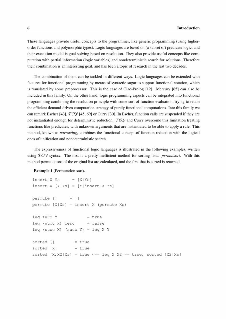
The expressiveness of functional logic languages is illustrated in the following examples, written

using T OY syntax. The first is a pretty inefficient method for sorting lists: permutsort. With this

method permutations of the original list are calculated, and the first that is sorted is returned.

Example 1 (Permutation sort).

insert X Ys = [X|Ys]

insert X [Y|Ys] = [Y|insert X Ys]

permute [] = []

permute [X|Xs] = insert X (permute Xs)

leq zero Y = true

leq (succ X) zero = false

leq (succ X) (succ Y) = leq X Y

sorted [] = true

sorted [X] = true

sorted [X,X2|Xs] = true <== leq X X2 == true, sorted [X2|Xs]

1.2 Functional logic programming 7

check L = L <== sorted L == true

sort L = check (permute L)

insert is a function that inserts an element nondeterministically in a list, so permute is also non-

deterministic. sorted is a deterministic function that checks if the given list is sorted, and check is a

function that returns the list passed as an argument if it is sorted. Finally, sort calculates a permutation

of L, and returns it if it is sorted. This example shows how the combination of nondeterminism (from

logic programming) and lazy evaluation (from functional programming) improves the efficiency. In a

purely logic language like Prolog, the same example is written as:

permutationSort(L,L2) :- permute(L,L2), sorted(L2).

Here, every candidate solution L2 is completely created before it is tested. In a purely functional lan-

guage, one usually follows the ’list of successes’ approach: generate the list of all possible solutions (the

permutations) and filter it (only those sorted). In the functional logic setting we still use a generator to

create the possible solutions one by one, as in a logic language. But the laziness allows us to generate

only a small fraction of the list, the minimum to be able to apply sorted. This way, the creation of a

list will be interrupted as soon as sorted recognizes it cannot lead to an ordered list. Therefore we do

not need to generate the whole list of candidates, as in a functional language, and we avoid checking dif-

ferent list with the same prefix; obtaining an important improvement in efficiency. For more information

about this example, see [25].

The following is another example of the expressiveness of functional logic languages. We can specify

the behavior of a function last that returns the last element of a list as: last l = e iff ∃xs. append xs [e] =l. Using a functional logic language we can easily define a function last:

Example 2 (Last element of a list [29]).

append [] Ys = Ys

append (X:Xs) Ys = X : (append Xs Ys)

last L = E <== (append Xs [E]) == L

Here we define append, the concatenations of lists, in the usual way. The function last is defined

directly from the specification, by means of a conditional equation. This equation states that the last

element of a list L is E if append Xs [E] is equal to L, where Xs and E are extra variables, i.e.,

8 Introduction

variables that appear in the right-hand side of the definition and not in the left-hand side. In this case,

functional logic languages provide search for solutions for these extra variables. For example, if we

want to reduce last [1,2,3] the system will instantiate Xs to [1,2] and E to 3, which satisfies the

condition append [1, 2] [3] = [1, 2, 3]; returning 3 as the last element.

Two surveys covering the integration of functional and logic languages can be found [28] and [29].

Besides, more information about functional logic programming in general can be found in Michael

Hanus’ web page [27].

1.3 Motivation

In this section we will explain the motivation of this work. As we have said before, the main motivation is

to solve a known problem with higher order (HO) patterns in functional logic languages. In the previous

work “Polymorphic Types in Functional Logic Programming” [24] this problem was detected, and the

solution was to forbid potentially problematic HO patterns. In this work we propose a more flexible

solution that admits patterns which were forbidden in [24]. A secondary motivation is to technically

clarify the different grade of polymorphism that can be given to local declarations. Implementations of

functional and functional logic languages vary significantly in this point, and they do not usually explain

nor formalize their choice.

1.3.1 Type problems with HO patterns in FLP

In our formalism patterns appear in the left-hand side of rules and in lambda or let expressions. Some of

these patterns can be HO patterns, if they contain partial applications of function or constructor symbols.

HO patterns can be a source of problems from the point of view of the types. In particular, it was shown

in [24] that unrestricted use of HO patterns leads to loss of subject reduction, an essential property for

a type system expressing that evaluation does not change types. The following is a crisp example of the

problem.

Example 3 (Polymorphic Casting [10]).Consider the program consisting of the rules {snd X Y → Y , and true X → X , and false X →false} with the usual types inferred by a classical Damas & Milner algorithm: {snd : ∀α, β.α →β → β, and : bool → bool → bool}. Then we can write the functions co (snd X) → X and

cast X → co (snd X), whose inferred types will be ∀α.∀β.(α → α) → β and ∀α.∀β.α → β

respectively. It is clear that the expression and (cast 0) true is well-typed, because cast 0 has type bool

1.3 Motivation 9

(in fact it has any type), but if we reduce that expression using the rule of cast the resulting expression

and 0 true is ill-typed.

In this case cast behaves as the usual identity function, returning the same element that accepts as

argument. But it permits us to “cast” the type of the element to any other type, making the type system

pretty useless.

The problem arises when dealing with HO patterns, because unlike FO patterns, knowing the type

of a HO pattern does not always permit us to know the type of its subpatterns. For example, given the

FO pattern (X, true) of type (int, bool), we know that the type of X must be int. The same happens

with [X, 0] of type [int]. On the other hand, knowing that the HO pattern snd X has type int → int

does not permit us to know anything about the type of X . X may have type int, bool, [int → bool] or

any other type, and the type of the whole patter will not change: int→ int. In the previous example the

cause of the type problems is function co, because its pattern snd X is opaque and shadows the type of

its subpattern X . Usual inference algorithms treat this opacity as polymorphism, and that is the reason

why it is inferred a completely polymorphic type for the result of the function co.

In [24] the appearance of any opaque pattern in the left-hand side of the rules is prohibited, but we

will see that it is possible to be less restrictive. The key is making a distinction between transparent and

opaque variables of a pattern: a variable is transparent if its type is univocally fixed by the type of the

pattern, and is opaque otherwise. We call a variable of a pattern critical if it is opaque in the pattern and

also appears elsewhere in the expression. The formal definition of opaque and critical variables will be

given in Chapter 3. With these notions we can relax the situation in [24], prohibiting only those patterns

having critical variables.

1.3.2 Variety of polymorphism in local definitions

Functional and functional logic languages provide syntax to introduce local definitions inside an expres-

sion. But in spite of the popularity of let expressions, different implementations treat them differently

because of the polymorphism they give to bound variables. This difference can be observed in Example

4, being (e1, . . . , en) and [e1, . . . , en] the usual tuple and list notation respectively.

Example 4 (let expressions).e1 ≡ let F = id in (F true, F 0)e2 ≡ let [F,G] = [id, id] in (F true, F 0, G 0, G false)

Intuitively, e1 gives a new name to the identity function and uses it twice with arguments of different

10 Introduction

types. Surprisingly, not all implementations consider this expression as well-typed, and the reason is that

F is used with different types in each appearance: bool → bool and int → int. Some implementations

as Clean 2.2, PAKCS 1.9.1 or KICS 0.81893 consider that a variable bound by a let expression must be

used with the same type in all the appearances in the body of the expression. In this situation we say that

lets are completely monomorphic, and write letm for it.

On the other hand, we can consider that all the variables bound by the let expression may have

different but coherent types, i.e., are treated polymorphically. Then expressions like e1 or e2 would be

well-typed. This is the decision adopted by Hugs Sept. 2006, OCaml 3.10.2 or F# Sept. 2008. In this

case, we will say that lets are completely polymorphic, and write letp.

Finally, we can treat the bound variables monomorphically or polymorphically depending on the

form of the pattern. If the pattern is a variable, the let treats it polymorphically, but if it is compound the

let treats all the variables monomorphically. This is the case of GHC 6.8.2, SML of New Jersey v110.67

or Curry Münster 0.9.11. In this implementations e1 is well-typed, while e2 not. We call this kind of let

expression letpm.

Programming language and version letm letpm letpGHC 6.8.2 ×

Hugs Sept. 2006 ×Standard ML of New Jersey 110.67 ×

Ocaml 3.10.2 ×F# Sept. 2008 ×

Clean 2.0 ×T OY 2.3.1* ×

Curry PAKCS 1.9.1 ×Curry Münster 0.9.11 ×

KICS 0.81893 ×(*) we use where instead of let, not supported by T OY

Figure 1.1: Let expressions in different programming languages

Figure 1.1 summarizes the decisions of various implementations of functional and functional logic

languages. The exact behavior wrt. types of local definitions is usually not well documented, not to say

formalized, in those systems. A sample of this can be found in GHC [3], a famous implementantion

of Haskell. They treated pattern bindings polymorphically (letp) but in July 2006 Simon Peyton Jones

changed experimentally the behavior to letpm, in order to check if people noticed it (and he only received

a few messages complaining). They have finally adopted the new choice, as can be seen in [55, 4]. Our

aim is to technically clarify this question by adopting a neutral position, and formalizing the different

possibilities for the polymorphism of local definitions.

1.4 Contributions 11

1.4 Contributions

In this work we have proposed a type system for functional logic languages based on Damas & Milner

type system. As far as we know, prior to our work only [24] treats with technical detail a type system for

functional logic programming. Our work makes clear contributions when compared to [24]:

• By introducing the notion of critical variables, we are more liberal in the treatment of opaque

variables, but still preserving the essential property of subject reduction. Moreover, this liberal-

ity extends also to data constructors, dropping the traditional restriction of transparency required

to them. This is somehow similar to what happens with existential types [49] or generalized

algebraic data types [57], a connection that we plan to further investigate in the future.

• Our type system considers local pattern bindings and λ-abstractions (also with patterns), that were

missing in [24]. In addition to that, we have made a rather exhaustive analysis and formalization

of different possibilities for polymorphism in local bindings.

• Subject reduction was proved in [24] wrt. a narrowing calculus. Here we do it wrt. an small-step

operational semantics closer to real computations.

• In [24] programs came with explicit type declarations. Here we provide algorithms for inferring

types for programs without such declarations, which can easily became part of the type stage of a

FL compiler.

Chapter 2

Preliminaries

In this section we will present some definitions and notation used in the rest of the work. We will begin

with the syntax of expressions and programs, and definitions about substitutions. Then we will treat

types, their syntax and some relations involving them. Finally, we will present sets of assumptions, the

way of storing type assumptions over symbols in our framework.

A global writing convention used in this work is that en is a sequence of n elements e1 . . . en, and eithe i− th element in that sequence.

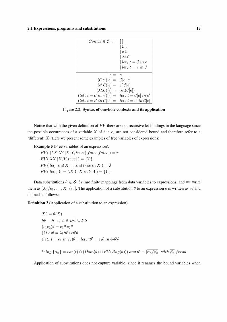
2.1 Expressions, programs and substitutions

We assume a signature Σ = DC ∪ FS where DC and FS are two disjoint sets of data constructor

and function symbols resp., all them with an associated arity. We write DCn and FSn for the set of

constructor and function symbols of arity n. We also assume a numerable set of data variables DV .

The syntax of the expressions of the language appears in Figure 2.1. Notice that λ-abstractions and

let expressions support patterns instead of single variables, and there are three different kinds of let

expressions: letm, letpm and letp; as explained in the previous chapter. We make a distinction between

the different expressions. X e1 . . . em (m ≥ 0) are called flexible expressions (variable application when

m > 0). On the other hand, rigid expressions have the form h e1 . . . em; they are called junk if h ∈ CSn

and m > n, active if h ∈ FSn and m ≥ n, and passive otherwise. Expressions like λt1 . . . tn.e will

be usually written as λtn.e, and we will write let∗ for any type of let expression: letm, letpm or letp.

As usual, expression application is left associative, so e1 e2 e3 is equal to (e1 e2) e3. We will use the

14 Preliminaries

metavariable h for any symbol in DC ∪ FS, and s for any symbol in DC ∪ FS ∪ DV .

Data variables DV X,Y,. . .Constructor symbol DC cFunction symbol FS fPatterns Pat 3 t ::= X

| c t1 . . . tn if c ∈ DCm and n ≤ m| f t1 . . . tn if f ∈ FSm and n < m

First Order pattern FOPat 3 fot ::= X| c fot1 . . . fotn if c ∈ DCn

Higher Order pattern HOPat 3 hot ::= h t1 . . . tm if h ∈ DCn ∪ FSn and m < n| c t1 . . . tn if c ∈ DCn and some ti ∈ HOPat

Expression Expr 3 e ::= X| c| f| (e1 e2)| λt.e if t is linear| letm t = e1 in e2 if t is linear| letpm t = e1 in e2 if t is linear| letp t = e1 in e2 if t is linear

Figure 2.1: Syntax of expressions

Contexts are expressions with exactly one hole, and are defined in Figure 2.2. The application of

contexts to expressions (written C[e]) is also defined in the same figure. Notice that context application

may capture variables, for example in (λX.[])X .

var(e) is the set of all the variables appearing in e. The set of free variables (FV ) of an expression

e is the set of all the variables in e not bounded by any λ-abstraction or let expression. The formal

definition is as follows.

Definition 1 (Free variables of an expression).

FV (X) = {X}FV (h) = ∅ if h ∈ DC ∪ FSFV (e1e2) = FV (e1) ∪ FV (e2)FV (λt.e) = FV (e) r var(t)FV (let∗ t = e1 in e2) = FV (e1) ∪ (FV (e2) r var(t))

2.1 Expressions, programs and substitutions 15

Contxt 3 C ::= [ ]| C e| e C| λt.C| let∗ t = C in e| let∗ t = e in C

[ ]e = e(C e′)[e] = C[e] e′(e′ C)[e] = e′ C[e](λt.C)[e] = λt.(C[e])

(let∗ t = C in e′)[e] = let∗ t = C[e] in e′(let∗ t = e′ in C)[e] = let∗ t = e′ in C[e]

Figure 2.2: Syntax of one-hole contexts and its application

Notice that with the given definition of FV there are not recursive let-bindings in the language since

the possible occurrences of a variable X of t in e1 are not considered bound and therefore refer to a

‘different’ X . Here we present some examples of free variables of expressions:

Example 5 (Free variables of an expression).FV ( (λX.λY.[X,Y, true]) false false ) = ∅FV ( λX.[X,Y, true] ) = {Y }FV ( letp snd X = snd true in X ) = ∅FV ( letm Y = λX.Y X in Y 4 ) = {Y }

Data substitutions θ ∈ Subst are finite mappings from data variables to expressions, and we write

them as [X1/e1, . . . , Xn/en]. The application of a substitution θ to an expression e is written as eθ and

defined as follows:

Definition 2 (Application of a substitution to an expression).

Xθ = θ(X)hθ = h if h ∈ DC ∪ FS(e1e2)θ = e1θ e2θ

(λt.e)θ = λ(tθ′).eθ′θ(let∗ t = e1 in e2)θ = let∗ tθ

′ = e1θ in e2θ′θ

being {αn} = var(t) ∩ (Dom(θ) ∪ FV (Rng(θ))) and θ′ ≡ [αn/βn] with βn fresh

Application of substitutions does not capture variable, since it renames the bound variables when

16 Preliminaries

there exists the risk of capture, i.e., they appear in FV (Rng(θ)). Notice that renaming is not performed

in e1 of let expressions. In this case, any variable in FV (e1) appearing in var(t) will not be bound,

because it will refer to a ’different’ variable. The following example presents some applications of

substitution to expressions:

Example 6 (Application of a substitution to an expression).(F id [1, 2, 3]) [F/map] = map id [1, 2, 3](λX.X + 1) [X/0] = λY.Y + 1((λX.X + 1) X) [X/0] = (λY.Y + 1) 0(letpm X = 1 in Z +X) [Z/1] = letpm X = 1 in 1 +X

(letp X = 1 in Z +X) [Z/X] = letp W = 1 in X +W

(letm X = X +X in X) [X/1] = letm Y = 1 + 1 in Y

We call domain of a substitution to the set of variables which are changed by the substitution:

Dom(θ) = {X ∈ DV|Xθ 6= X}. We call range of a substitution to the set Rng(θ) = {Xθ|X ∈Dom(θ)}. Given two substitutions θ1 and θ2, the composition of substitutions is another substitution

denoted as θ1θ2 and defined as Xθ1θ2 = (Xθ1)θ2. The simultaneous composition of two substitutions

θ1 and θ2 is defined only when the domains are disjoint, i.e., when Dom(θ1) ∩ Dom(θ2) = ∅. In this

case, the simultaneous composition of θ1 and θ2 is written as (θ1 + θ2) and is defined as:

X(θ1 + θ2) =

{Xθ1 if X ∈ Dom(θ1)Xθ2 otherwise

If A is a set of variables, the restriction of a substitution θ1 to A (θ1|A) is defined as:

X(θ1|A) =

{Xθ1 if X ∈ AX otherwise

The most important data substitutions used in this work are pattern-substitutions, those substitutions

such that their range are patterns instead of expressions. We denote this set of substitutions as PSubst ={θ ∈ Subst|Rng(θ) ∈ Pat}.

A program rule is defined as PRule 3 r ::= f t1 . . . tn → e where n ≥ 0, the set of patterns

{t1, . . . , tn} is linear (i.e., every variable appears only once in all the patterns) and FV (e) ⊆⋃i var(ti).

Therefore, extra variables (variables that appear in the right-hand side and do not appear in any of the

patterns of the left-hand side) are not considered in this work. A program P is a set of zero or more

program rules, Prog 3 P = {r1, . . . , rn} with n ≥ 0. The union of programs is denoted as P1 ∪ P2.

2.2 Types 17

2.2 Types

Types are the kind of objects that the type system will relate with expressions. In oder to define them

we assume a numerable set of type variables T V and a countable alphabet T C =⋃n∈N T C

n of type

constructors. As data constructors, type constructors have an associated arity. The syntax of types can

be found in Figure 2.3. Sometimes we will refer to a simple type τ only as “type”, but in these cases

the context will make clear the meaning. Usually, a type-scheme ∀α1.∀α2 . . . ∀αn.τ will be written as

∀α1, α2, . . . , αn.τ or simply ∀αn.τ . As usual, the arrow→ is right associative, so int → int → int is

equal to int→ (int→ int).

Type variable T V α, β, γ, . . .

Simple type SType 3 τ ::= α| C τ1 . . . τn with C ∈ T Cn| τ1→ τ2

Type-scheme TScheme 3 σ ::= τ| ∀α.σ

Figure 2.3: Syntax of the types

The set of free type variables of a type-scheme is the set of all the type variable not bound by any

quantifier. The formal definition is as follows.

Definition 3 (Free type variables of a type-scheme).

FTV (α) = {α}FTV (C τ1 . . . τn) =

⋃i FTV (τi)

FTV (τ1 → τ2) = FTV (e1) ∪ FTV (e2)FTV (∀αn.τ) = FTV (τ) r {αn}

As we have done with data substitutions, we define type substitutions as finite mappings from type

variables to simple types (not type-schemes): [α1/τ1, . . . , αn/τn]. These substitutions will be referred

as π, and the set of all these substitutions as T Subst. The application of type substitutions over variables

and types is the usual, and over type-schemes is the application only over their free type variables. Based

on substitutions, we can define two important relations over type-schemes: instance and generic instance.

The difference between them is that instantation only replaces free type variables by simple types, and

generic instantation replaces only the quantified variables, i.e., those understood polymorphically, by

simple types. Therefore the generic instances of a type-scheme are all the simple types represented by

18 Preliminaries

that type-scheme.

Definition 4 (Instance of a type-scheme).We say that σ′ is an instance of σ if σ′ = σπ for some π ∈ T Subst.

For example, bool→ bool is an instance of α→ α and ∀α.α→ int is an instance of ∀α.α→ β.

Definition 5 (Generic instance of a type-scheme σ).τ is a generic instance of a type-scheme σ ≡ ∀αn.τ ′ (or σ subsumes τ , or σ is more general than

τ ) if τ ≡ τ ′[αn/τn] for some types τn. We represent that σ � τ . We extend � to a relation between

type-schemes by saying that σ � σ′ iff for every type τ such that σ′ � τ then σ � τ . Notice that with

simple types τ � τ ′ iff τ ≡ τ ′.

Examples:

• ∀α.α→ α � bool→ bool

• ∀α.α→ α � ∀β.∀γ.(β, γ)→ (β, γ)• (α, int) � (α, int)• ∀α.∀β.[α]→ [β]→ [(α, β)] � ∀γ.[γ → bool]→ [δ]→ [(γ → bool, δ)]

There exists a useful characterization of � with a more operational behavior which is explained in

[19, 62]. This characterization is presented in the following proposition.

Proposition 1 (Characterization of �).A type-scheme ∀α1 . . . αn.τ � ∀β1 . . . βm.τ

′ iff

1.- there is a type substitution π ≡ [αn/τn] (for some types τ1 . . . τn) such that τ ′ ≡ τπ2.- β1 . . . βm do not occur free in ∀α1 . . . αn.τ

The proof of the correctness of this characterization can be found in [19].

Notice that � is a reflexive and transitive relation. Therefore we can define an equivalence relation

between type-schemes in the following way.

Definition 6 (Equivalence between type-schemes).σ ≡� σ′ ⇐⇒def σ � σ′ ∧ σ′ � σ.

Clearly the relation ≡� is reflexive, symmetric and transitive. We will usually refer to it simply as

=. The last useful notion about types is that of variant of a type-scheme. This notion is needed when

formalizing the inference relation (Chapter 4).

2.2 Types 19

Definition 7 (Variant of a type-scheme).We say that a type τ ′ is a variant of a type-scheme σ ≡ ∀αn.τ if τ ′ ≡ τ [αn/βn] with βn fresh type

variables. We usually write it as σ �var τ ′.

Intuitively, a variant of a type-scheme is a simple type where all the quantified variables have been

replaced by variables which have not been used before. Examples of variants are ∀α.α→ α �var β → β

and ∀α.α → β → (α, β) �var γ → β → (γ, β). Now we will present two remarks that come from

the previous definitions. The first one is related to the equivalence of α-converted type-schemes, and the

second is about the fact that generic instances have more free type variables.

Remark 1.Note that ∀αn.τ ≡� ∀βn.τ [αn/βn] if {βn}∩FTV (τ) = ∅. In other words, two different type-schemes

are the same if we change the bounded variables for other variables which do not appear free in τ . For

example, ∀α, β.(α, β)→ α is equal to ∀γ, δ.(γ, δ)→ γ.

Remark 2.If σ � σ′ then FTV (σ) ⊆ FTV (σ′).

It is clear from the characterization of� given in Proposition 1. If α is a type variable in FTV (σ) then it

will not be affected by π. Besides it will not be generalized, i.e., α will be different from the generalized

variables βj . Therefore α ∈ FTV (σ′) and α ∈ FTV (σ) =⇒ α ∈ FTV (σ′), so FTV (σ) ⊆ FTV (σ′).

Sets of assumptions are the constructions that relate types-schemes to symbols in our type system.

They are not only important in type derivations, but they are key in type inference because they also

“store” the type constraints found for every symbol.

Definition 8 (Set of assumptions).A set of assumptions is a set of the form {s1 : σ1, . . . , sn : σn}, where si is a function symbol, data

constructor symbol or variable and σi is a type-scheme. We usually denote a set of assumptions with A.

We can view A as a partial function defined as:

A(s) =

{σ if {s : σ} ∈ Aundefined otherwise

Sets of assumptions can be extended with new assumptions over new or existing symbols. If the

symbol does not appear in the original set of assumptions, the new assumption is added; otherwise the

previous assumption is discarded and then the new assumption is added.

Definition 9 (Adding an assumption to A).Let As be the set resulting of discarding all the assumptions over the symbol s in A. Then adding the

20 Preliminaries

assumption {s : σ} to A is defined as A ⊕ {s : σ} = As ∪ {s : σ}. This notion is extended to adding

sets of assumptions in the usual way: A⊕ {sn : σn} = A⊕ {s1 : σ1} ⊕ . . .⊕ {sn : σn}.

⊕ operator is left associative, so A ⊕ {s : σ} ⊕ {s′ : σ′} = (A ⊕ {s : σ}) ⊕ {s′ : σ′}. Notice

that it does not matter the order when adding assumptions over different symbols: the resulting set of

assumptions is the same.

Remark 3.If s 6= s′ thenA⊕{s : σ}⊕{s′ : σ′} is the same asA⊕{s′ : σ′}⊕{s : σ}. This remark can be extended

to sets of assumptions, in the sense that A⊕ {Xn : σn} ⊕ {X ′m : σ′m} = A⊕ {X ′m : σ′m} ⊕ {Xn : σn}if Xi 6= X ′j for 1 ≤ i ≤ n and 1 ≤ j ≤ m.

The previous notion of free type variables is easily extended to set of assumptions: the free type

variables of a set of assumptions A are the free type variables in all the type-schemes appearing in A.

This notion if formally defined as follows:

Definition 10 (Free type variables of A).FTV ({sn : σn}) =

⋃ni=1 FTV (σi)

To finish this section we will present the important notion of generalization of a type to obtain a

type-scheme. This operation is used in type derivation and is essential to support polymorphism.

Definition 11 (Generalization of τ wrt. A).Gen(τ,A) = ∀α1 . . . ∀αn.τ where {α1, . . . , αn} = FTV (τ) r FTV (A).

Examples:

• Gen([int], {true : bool, false : bool, f : α→ α}) = [int]• Gen(α, {true : bool, false : bool}) = ∀α.α• Gen(α, {true : bool, false : bool, f : α→ α}) = α

• Gen(α→ β, {true : bool, false : bool, f : α→ α}) = ∀β.α→ β

As can be seen, the generalization of a type τ is the type-scheme resulting of quantifying all the type

variables not appearing free in A. Then it is clear that it depends only on the free type variables of the

set of assumptions, not in the particular set of assumptions involved, as the following remark states.

Remark 4.If FTV (A) = FTV (A′) then Gen(τ,A) = Gen(τ,A′)

Chapter 3

Type Derivations

Type derivations (or type judgements) allow us to relate a type with an expression. This type can be

unique, if the expression is monomorphic; or multiple, if the expression is polymorphic. In this section

we present two typing relations based on Damas & Milner type system but handling appropriately HO

patterns and the different kinds of local definitions.

3.1 Rules of the type system

We have found convenient to separate the task of giving a regular Damas & Milner type to an expression

and the task of checking critical variables, as discussed in Section 1.3.1. The first task is performed by the

typing relation `, which also handle the different kinds of local definitions; and the second by `•. Notice

that these relations permit us to derive types for expression, not programs. This is not a problem because

as we will see in Section 3.3 the notion of well-typed program will be defined using these relations over

expressions.

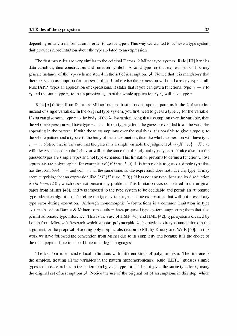
3.1.1 Basic typing relation `

The rules of the basic typing relation ` appear in Figure 3.1. All the rules have been designed allowing

compound patterns in λ-abstractions and let expressions. This is a feature implemented in existing

languages but rarely expressed directly in the formalization of their type systems. We have made the

effort of keeping explicitly the treatment of these compound patterns inside the type system, instead of

22 Type Derivations

[ID]A ` s : τ

ifs ∈ DC ∪ FS ∪ DV∧ A(s) = σ ∧ σ � τ

[APP]A ` e1 : τ1 → τA ` e2 : τ1A ` e1e2 : τ

[Λ]A⊕ {Xn : τn} ` t : τtA⊕ {Xn : τn} ` e : τA ` λt.e : τt → τ

if {Xn} = var(t)

[LETm]

A⊕ {Xn : τn} ` t : τtA ` e1 : τt

A⊕ {Xn : τn} ` e2 : τ2A ` letm t = e1 in e2 : τ2

if {Xn} = var(t)

[LETXpm]A ` e1 : τ1

A⊕ {X : Gen(τ1,A)} ` e2 : τ2A ` letpm X = e1 in e2 : τ2

[LEThpm]

A⊕ {Xn : τn} ` h t1 . . . tm : τtA ` e1 : τt

A⊕ {Xn : τn} ` e2 : τ2A ` letpm h t1 . . . tm = e1 in e2 : τ2

if {Xn} = var(t1 . . . tm)

[LETp]

A⊕ {Xn : τn} ` t : τtA ` e1 : τt

A⊕ {Xn : Gen(τn,A)} ` e2 : τ2A ` letp t = e1 in e2 : τ2

if {Xn} = var(t)

Figure 3.1: Rules of the type system

3.1 Rules of the type system 23

depending on any transformation in order to derive types. This way we wanted to achieve a type system

that provides more intuition about the types related to an expression.

The first two rules are very similar to the original Damas & Milner type system. Rule [ID] handles

data variables, data constructors and function symbol. A valid type for that expressions will be any

generic instance of the type-scheme stored in the set of assumptions A. Notice that it is mandatory that

there exists an assumption for that symbol in A, otherwise the expression will not have any type at all.

Rule [APP] types an application of expressions. It states that if you can give a functional type τ1 → τ to

e1 and the same type τ1 to the expression e2, then the whole application e1 e2 will have type τ .

Rule [Λ] differs from Damas & Milner because it supports compound patterns in the λ-abstraction

instead of single variables. In the original type system, you first need to guess a type τx for the variable.

If you can give some type τ to the body of the λ-abstraction using that assumption over the variable, then

the whole expression will have type τx → τ . In our type system, the guess is extended to all the variables

appearing in the pattern. If with those assumptions over the variables it is possible to give a type τt to

the whole pattern and a type τ to the body of the λ-abstraction, then the whole expression will have type

τt → τ . Notice that in the case that the pattern is a single variable the judgment A⊕ {X : τx} ` X : τxwill always succeed, so the behavior will be the same that the original type system. Notice also that the

guessed types are simple types and not type-schemes. This limitation prevents to define a function whose

arguments are polymorphic, for example λF.(F true, F 0). It is impossible to guess a simple type that

has the form bool → τ and int → τ at the same time, so the expression does not have any type. It may

seem surprising that an expression like (λF.(F true, F 0)) id has not any type, because its β-reduction

is (id true, id 0), which does not present any problem. This limitation was considered in the original

paper from Milner [48], and was imposed to the type system to be decidable and permit an automatic

type inference algorithm. Therefore the type system rejects some expressions that will not present any

type error during execution. Although monomorphic λ-abstractions is a common limitation in type

systems based on Damas & Milner, some authors have proposed type systems supporting them that also

permit automatic type inference. This is the case of HMF [41] and HML [42], type systems created by

Leijen from Microsoft Research which support polymorphic λ-abstractions via type annotations in the

argument; or the proposal of adding polymorphic abstraction to ML by Kfoury and Wells [40]. In this

work we have followed the convention from Milner due to its simplicity and because it is the choice of

the most popular functional and functional logic languages.

The last four rules handle local definitions with different kinds of polymorphism. The first one is

the simplest, treating all the variables in the pattern monomorphically. Rule [LETm] guesses simple

types for those variables in the pattern, and gives a type for it. Then it gives the same type for e1 using

the original set of assumptions A. Notice the use of the original set of assumptions in this step, which

24 Type Derivations

prevents recursive definitions. If a variable X appears in the pattern and in e1, the type for the second

occurrence will come from A, independently of the type guessed in the first step, i.e., the occurrences

will refer to different variables X . Finally the set of assumptions extended with the guessed types for the

variables is used to give a type for e2, which will be the type of the whole expression. Rule [LETXpm]handle the case of a letpm expression with a single variable as a pattern, the situation in which it will

be treated polymorphically. First it gives a simple type τ1 to e1, and then it gives a type τ2 for e2 using

the original A extended with an assumption that relates the variable with the generalization of τ1 wrt.

A. It is this generalization step (Definition 11) which provides the polymorphism to the variable. The

key resides in the fact that if you can give a type for an expression containing type variables which

do not appear in the set of assumptions, you can also give to that expression any other type in which

those type variables have been replaced by simple types. If we replace X by e1 in e2, each occurrence

of e1 could have different types in the previous way. Then the generalization step quantifies the type

variables which do not appear free in A, those that could be any type, generating a type-scheme whose

generic instances will be all the possible types for e1. With this assumption, X will behave like e1 and its

potential polymorphism. Rule [LEThpm] is the same as [LETm] because letpm treats compound patterns

monomorphically. Finally, rule [LETp] behaves like [LETXpm] but extends the polymorphism to all the

variables in the pattern. It needs an additional step to check that the guessed types for the variables give

a valid type to pattern that is the same as the type for e1. Notice that in this case the generalization

may lose the connection between the guessed types for the variables. This can be seen in the expression

letp [F,G] = [id, id] in (F 0, G true), whose type derivation appears in Example 7-4). The type for

both F and G can be α → α (being α a variable not appearing in A), but the generalization step will

assign both the type-scheme ∀α.α → α. This will allow us to derive a type int → int for F and

bool → bool for G, yielding a type (int, bool) for the whole expression. The difference between the

two types might seem surprising, because both F and G appear in the same list, but it can be easily

understood if we see the pattern matching as projection functions. The list [id, id] has the polymorphic

type ∀α.[α→ α]. When we project the first element we can assume that [id, id] has type [int→ int], so

F has type int → int. But when we project the second element, we can freely assume that [id, id] has

type [bool→ bool], because it is polymorphic, and that is why G can have type bool→ bool.

Here we show some examples of type derivations:

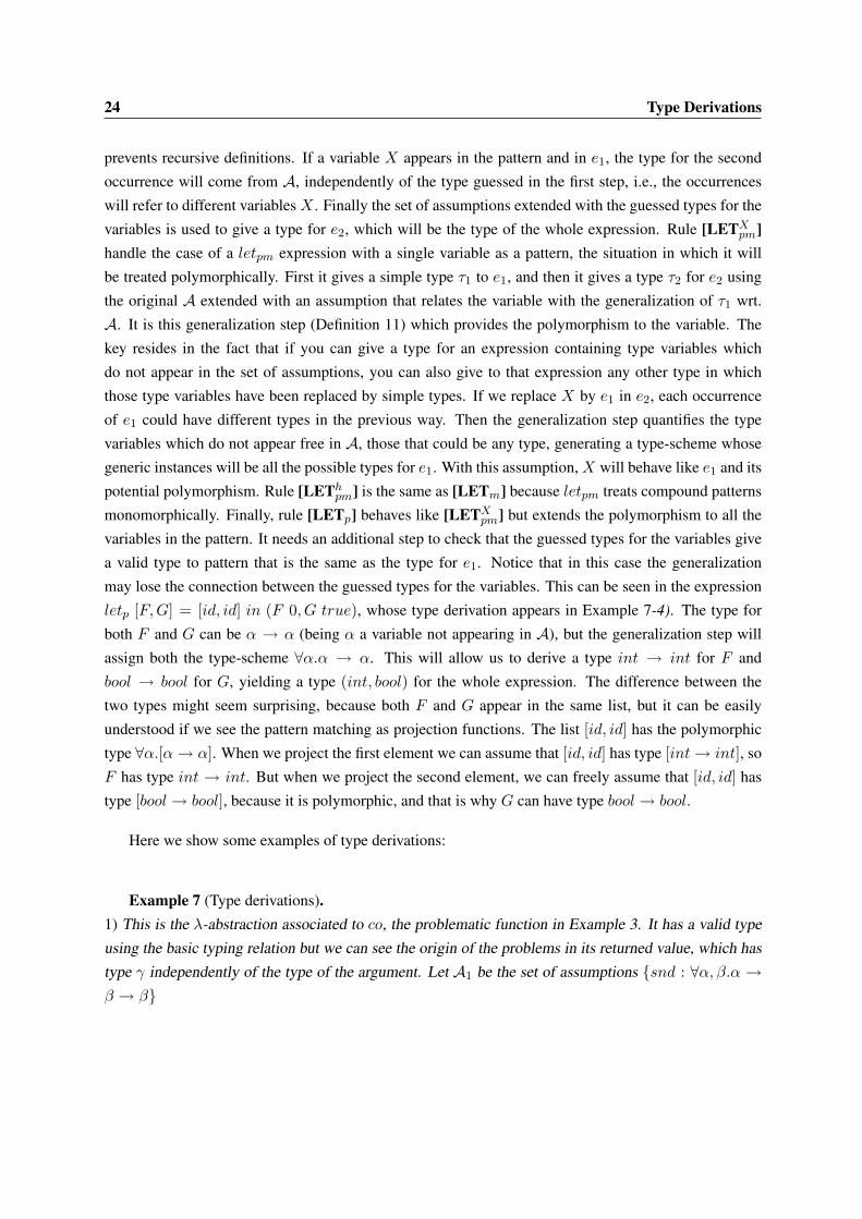
Example 7 (Type derivations).1) This is the λ-abstraction associated to co, the problematic function in Example 3. It has a valid type

using the basic typing relation but we can see the origin of the problems in its returned value, which has

type γ independently of the type of the argument. Let A1 be the set of assumptions {snd : ∀α, β.α →β → β}

3.1 Rules of the type system 25

[Λ][APP]

[ID]A1 ⊕ {X : γ} ` snd : γ → δ → δ

[ID]A1 ⊕ {X : γ} ` X : γ

A1 ⊕ {X : γ} ` snd X : δ → δ[ID]

A1 ⊕ {X : γ} ` X : γ

A1 ` λsnd X.X : (δ → δ)→ γ

2) The following is an example of completely monomorphic let. F has type int → int, so it can

only be applied to expressions of type int. Let A2 be the set of assumptions {id : ∀α.α→ α, 0 : int}

[LETm][ID]

A2 ⊕ {F : int→ int} ` F : int→ int[ID] A2 ` id : int→ int

[APP](. . .)

A2 ⊕ {F : int→ int} ` F 0 : int

A2 ` letm F = id in F 0 : int

3) The next example shows the polymorphism of letpm expressions when the pattern is a variable.

Here F has a polymorphic type ∀γ.γ → γ when deriving the type of (F 0, F true), so it can be used

with types int→ int and bool→ bool. LetA3 be the set of assumptions {id : ∀α.α→ α, 0 : int, true :bool, ()1 : ∀α, β.α→ β → (α, β)}

[LETXpm]

[ID] A3 ` id : γ → γ[APP]

(. . .)A3 ⊕ {F : ∀γ.γ → γ} ` (F 0, F true) : (int, bool)

A3 ` letpm F = id in (F 0, F true) : (int, bool)

4) The following example is very similar to the previous one but using a letp expression. It shows

how variables that occur in the same list pattern are used with different types in the body of the let

expressions. Let A4 be the set of assumptions {id : ∀α.α → α, 0 : int, true : bool, ()1 : ∀α, β.α →β → (α, β), [ ] : ∀α.[α], cons : ∀α→ [α]→ [α]}

[LETp][APP]

(. . .)

A4 ⊕ {F : γ → γ,G : γ → γ} ` [F,G] : [γ → γ][APP]

(. . .)

A4 ` [id.id] : [γ → γ][APP]

(. . .)

A′4 ` (F 0, G true) : (int, bool)

A4 ` letp [F,G] = [id, id] in (F 0, G true) : (int, bool)

being A′4 ≡ A4 ⊕ {F : ∀γ.γ → γ,G : ∀γ.γ → γ}

Other of our aims when designing the type system has been to obtain syntax-directed type judgments.

In the original Damas & Milner type system [20] appear two rules, INST and GEN, that can occur

anywhere in the type judgement. The type system relates expressions with type-schemes, and these rules

allow to obtain generic instances and more general type-schemes from previous ones. Since these rules

can appear anywhere in the type derivation, it does not depend on the form of the expression. To solve

this problem we will eliminate these two rules and integrate into the others. As [62, 17] say, limiting the

type relation to simple types instead of type-schemes, any derivation can be build using GEN just before

the rule of LET (to obtain a general type for the variables) and INST before the rule for the symbols

(to obtain a generic instance). Therefore we have integrated the instantation step into the rule [ID],

1tuple constructor of arity 2

26 Type Derivations

which gives generic instances only; and the generalization step in the rules [LETXpm] and [LETp], those

supporting polymorphism. This way given an expression there is only one typing rule that can be used,

so the form of the type derivation depends only on the syntax of the expression.

3.1.2 Extended typing relation `•

The previous basic type relation ` gives a type to an expression, handling the different kinds of poly-

morphism in let expressions and the occurrences of compound patterns instead of single variables. In

this section we introduce the extended typing relation `• that uses the previous one to give types to ex-

pressions but also enforces the absence of critical variables, i.e., opaque variables which are “used” in

the expression. As we have seen in Section 1, the intuition behind an opaque variable is that is a data

variable of a pattern in a λ-abstraction or let expression whose type is not univocally fixed by the type

of the pattern. The problem arises in that due to this opacity we can build type derivations which assigns

incorrect assumptions to the variables. Let us illustrate this by an example:

Example 8.Let A be the set of assumptions {snd : ∀α, β.α → β → β, true : bool, 0 : int} and let e be the

expression letp snd X = snd true in X . A possible type derivation for this expressions is:

[LETp]

A⊕ {X : int} ` snd X : int→ intA ` snd true : int→ intA⊕ {X : int} ` X : int

A ` letp snd X = snd true in X : int

The problem here is since X is opaque, the fact that snd X and snd true have the same type does not

provide any information about that the assumption {X : int} is correct, and we have the false impression

that it is a valid assumption. Instead of int we could have given to X any other type, and we would have

obtain an expression that returns true with any type. A similar situation appears in λ-abstractions.

In [24] it is assumed that expressions contain only transparent patterns. In this framework, type

signatures for constructors and functions are part of the signature of the program. A type τm → τ is called

m-transparent if FTV (τm) ⊆ FTV (τ), and a function f is m-transparent if its type is m-transparent.

Then, a pattern h tn (with h ∈ DC ∪ FS) is called transparent if h is n-transparent and tn are also

transparent patterns; and opaque otherwise. In this framework patterns as snd X or snd true are opaque,

because in both cases snd is applied to one expression, and snd is not 1-transparent, so they are not valid

patterns in the left-hand side of the rules. We have found that this restriction can be relaxed, because

an opaque pattern can contain subpatterns whose type is actually fixed by the type of the whole pattern.

The problem with opaque variables arises when they are “used” in the expression, as in the previous

3.1 Rules of the type system 27

example. But if a variable is not “used” in the body, for example in letp snd X = snd true in true, the

assumption will not be used in the type derivation. Then, only the occurrence of opaque variables that

are “used” in the expression (i.e., are critical) must be checked.

In order to introduce the extended typing relation `• we need first to formally define opaque and

critical variables. The notion of opaque variable of a pattern relies on the typing relation `, as the

following definition states:

Definition 12 (Opaque variable of t wrt. A).Let t be a pattern that admits type wrt. a given set of assumptions A. We say that Xi ∈ {Xn} = var(t)is opaque wrt. A iff ∃τn, τ s.t. A⊕ {Xn : τn} ` t : τ and FTV (τi) * FTV (τ).

Examples:• X is an opaque variable in snd X when A contains the usual type assumption for snd : ∀α →β → β ). In this case we can build the type derivation A⊕ {X : γ} ` snd X : δ → δ and clearly

FV (γ) * FV (δ → δ).

• The tuple pattern (X,Y ) does not have any opaque variable, assuming the usual type for the tuple

constructor. In this case it is not possible to create a type derivation in which the types of the

variables X and Y do not appear in the type of the whole pattern.

• X is not opaque in snd [X, true] according to the usual type assumptions for snd and list con-

structors. Although the type of the argument of snd does not appear in the type of the whole

pattern, the type of X is fixed to bool by the subpattern [X, true] where it appears.

Since it is based on the existence of a certain type derivation, Definition 12 cannot be used as an

effective check for the opacity of variables. But it is possible to exploit the close relationship between

` and type inference � that will be presented in Chapter 4. Since � can be viewed as an algorithm,

Proposition 2 provides a more operational characterization of opaque variable which is useful when

implementing the type system.

Proposition 2 (Alternative characterization of opaque variable).Let t be a pattern that admits type wrt. a given set of assumptions A. We say that Xi ∈ {Xn} = var(t)is opaque wrt. A iff A⊕ {Xn : αn} � t : τg|πg and FTV (αiπg) * FTV (τg).

The proof of the equivalence of Definition 12 and Proposition 2 can be found in Lemma 4 of Ap-

pendix A. As we have seen, not all opaque variables are problematic, but only those that are “used” in

the expression. In this work we consider the simplest notion of “use”: a variable is used if it occurs in

the body of a λ-abstraction or let expression. More complex notions can be developed, based on static

28 Type Derivations

analysis of the program rules. For example given the program {const X → 0} and the expression

letp snd X = snd true in const X the variableX will not be used, even though it occurs in the body of

the let expression. In this case there will not be problematic that opacity avoids us to know the type ofX ,

because no pattern matching will be performed with it. Notice that knowing if a matched variable will

be effectively used in a computation is an undecidable problem, so an approximation must be chosen.

Once that we have a notion of “used variable”, we can define formally the notion of critical variables

of an expression wrt. a set of assumptions. In the following definition we present critical variables

considering our simple notion of “used variable”. For more complex notions the definition is the same

but replacing FV (..) by the particular check.

Definition 13 (Critical variables of e wrt. A).

critV arA(s) = ∅critV arA(e1e2) = critV arA(e1) ∪ critV arA(e2)critV arA(λt.e) = (opaqueV arA(t) ∩ FV (e)) ∪ critV arA(e)critV arA(let∗ t = e1 in e2) = (opaqueV arA(t) ∩ FV (e2)) ∪ critV arA(e1) ∪ critV arA(e2)

Examples:• As we have seen in the examples of the definition of opaque variables (Definition 12), X is opaque

in snd X . Therefore critV arA(λsnd X.X) = {X} because X appears in the body of the λ-

abstraction.

• Although X is opaque in snd X , critV arA(letm snd X = snd true in 0) = ∅ because X does

not occur in the rest of the expression.

• As we have seen beforeX is not opaque in snd [X, true], so trivially critV arA(λsnd [X, true].X) =∅.

With the previous definitions we can now formalize the extended typing relation. It only contains

one rule, [P] (Figure 3.2). This typing relation uses the basic one to give a type to an expression, and

then checks the absence of critical variables. Here we show some examples of type derivations with the

[P]A ` e : τA `• e : τ

if critV arA(e) = ∅

Figure 3.2: Rule of the extended type system

extended relation `•:

3.2 Properties of type derivations 29

Example 9 (Extended type derivations).

1. LetA1 be {snd : ∀α, β.α→ β → β}. ThenA1��̀•λsndX.X because althoughA1 ` λsndX.X :

(δ → δ)→ γ (from Example 7-1) we have seen that critV arA1(λsnd X.X) = {X}.

2. Using A2 ≡ {snd : ∀α, β.α → β → β, true : bool}, A2 `• λsnd X.true : (δ → δ) → bool

because A2 ` λsnd X.true : (δ → δ)→ bool and X is not critical in the expression.

3. A3 `• letpm F = id in (F 0, F true) : (int, bool), since A3 ` letpm F = id in (F 0, F true) :(int, bool) (from Example 7-3) and there are not critical variables in the expression.

3.2 Properties of type derivations

The typing relations fulfill a set of useful properties. Here we will use `? for any of the two typing

relations: ` or `•.

Theorem 1 (Properties of the typing relations).

a) If A `? e : τ then Aπ `? e : τπ, for any π ∈ T Subst

b) Let s be a symbol not appearing in e. Then A `? e : τ ⇐⇒ A⊕ {s : σs} `? e : τ .

c) If A⊕ {X : τx} `? e : τ and A⊕ {X : τx} `? e′ : τx then A⊕ {X : τx} `? e[X/e′] : τ .

d) If A⊕ {s : σ} ` e : τ and σ′ � σ, then A⊕ {s : σ′} ` e : τ .

Part a) states that type derivations are closed under type substitutions, i.e., from an instance of the

set of assumptions we can derive a type that is an instance of the original. b) shows that type derivations

for e depend only on the assumptions for the symbols in e. Then we can add or delete assumptions over

symbols not appearing in the expression and the type derivations will remain valid. c) is a substitution

lemma stating that in a type derivation we can replace a variable by an expression with the same type.

Finally, d) establishes that from a valid type derivation we can change the assumption of a symbol for a

more general type-scheme, and we still have a correct type derivation for the same type. Notice that this

is not true wrt. the typing relation `• because a more general type can introduce opacity. For example

the variable X is not opaque in snd X with the type bool → bool → bool for snd, but with a more

general type such as ∀α, β.α→ β → β X will be opaque.

30 Type Derivations

3.3 Subject reduction

Subject reduction is a key property for type systems, meaning that evaluation does not change the type of

an expression. This ensures that run-time type errors will not occur. Examples of this kind of errors are

adding two boolean expressions (true+ true) or applying the logical and function to integers (and 0 0).

Notice that partial functions can produce pattern matching errors during execution. An example of this

is the function head, which returns the first element of a list. This function is usually defined only for

non empty lists. Applying head to an empty list [] will usually yield to a pattern matching error, but this

is not considered a run-time type error, so the subject reduction property does not assures the absence

of this kind of run-time errors. Although in essence both errors are the same, calling a function with

an argument such that there is not any matching rule, the cause is different. In the former cases the

arguments have a different type that the expected, so it will be impossible to find a rule to reduce the

expression. In the latter case, the impossibility resides in the partiality of the function, but the arguments

have the correct type.

To state a subject reduction property we need two ingredients. First, a way of recognize those pro-

gram that are consistent with the type system. Second, a notion of evaluation to reduce expressions, i.e.,

a semantics. We will also need a transformation to adapt the syntax of our expressions to the semantics.

All these parts will be explained in the next sections.

3.3.1 Notion of well-typed program

Subject reduction is only guaranteed for well-typed programs, i.e., programs that are consistent with the

type system.

Definition 14. [Well-typed rule]

A program rule f t1 . . . tn → e is well-typed wrt. A if A `• λt1 . . . λtn.e : τ and τ is a variant of A(f).

Definition 15. [Well-typed program]

A program P is well-typed wrt. A if all its rules are well-typed wrt. A. If P is well-typed wrt. A we

write wtA(P).

Notice the use of the extended typing relation `• in the definition of well-typed rule. This is essential

to guarantee subject reduction, as we will explain later. The use of `• prevents us to consider the

problematic program in Example 3 as well-typed with the usual assumptions. Since λsnd X.X does

not have any type wrt. `• (as can be seen in Example 9-1), the rule of co is not well-typed. Although

3.3 Subject reduction 31

the restriction that the type of the lambda abstraction associated to a rule must be a variant of the type

of the function symbol (and not an instance) might seem strange, it is necessary. Otherwise, the fact

that a program is well-typed will not give us important information about functions like the type of their

arguments/result, or the number of arguments; and it will make us to consider as well-typed undesirable

programs. These situations are illustrated in Examples 10 and 11.

Example 10.Let P be the program {f true→ true, f 0→ true} and A be the set of assumptions {true : bool, 0 :int; f : ∀α.α → bool}. With the relaxed restriction we could affirm that P is well typed wrt A, which

is contrary to our intention and intuition. With parametric polymorphism the meaning of the assumption

f : ∀α.α → bool is that f is a function whose argument can have any type and whose result is of type

bool. Here this is false because f cannot accept any kind of argument (in contrast with the parametric

function id), but only bool or int.

Then the restriction assures that if in a rule an argument (or the result) is of a certain type, in all the

other rules this argument must have the same type.

Example 11.Let P be the program {fst X Y → X} andA be the set of assumptions {f : ∀α, β.α→ β}. If we relax

the mentioned restriction we could affirm that wtA(P) because A ` λX.λY.X : γ → δ → γ, and this

type is a generic instance of ∀α, β.α → β. Looking at the assumptions, we expect f to have only one

argument, which is not true. Using the original restriction, if we want A to make P well typed, it will

need to contain the assumption {f : ∀α, β.α → β → α} (or any generic instance), which indicates the

number of arguments of the function f .

Furthermore, relaxing this restriction every program with rules that admit any type will be consid-

ered well-typed using the assumption ∀α.α for all its function symbols. A final reason supporting the

restriction of the variant can be seen in the next example. Although it is somehow artificial, it shows that

subject reduction cannot be guaranteed in well-typed programs without the mentioned restriction.

Example 12.Suppose the program P ≡ {f X → g X} and the set of assumptions A ≡ {f : ∀α.α → α, g : β →β, true : bool}. If the definition of well-typed program is relaxed to not check that the types of the rules

are variants but generic instances, P will be well-typed wrt. A because λX.g X has type β → β, which

is a generic instance of the type of f : ∀α.α→ α. The expression f true has type bool, but if we use this

well-typed program to reduce it to g true the obtained expression is ill-typed, since true has not type β.

Although not explicitly stated, in [24] the same restriction is implicitly considered in the definition

of a well-typed defining rule for a function. This restriction is achieved by forcing the arguments tn and

32 Type Derivations

the result r in the rule f tn → r to have the same type (τi and τ respectively) that appear in the declared

type of f : τn → τ . These declared types have not quantification, but they are understood as universally

quantified, so they establish the same restriction that the variants in our case.

3.3.2 Semantics

In this work we consider the let-rewriting relation of [44]. This is strongly equivalent to HOCRWL [23],

a previously existing semantic framework for programs with HO non-deterministic functions. But it has

an important advantage: unlike HOCRWL, let-rewriting provides an operational behavior, representing

computations in a more natural way. In this work we have made two minor changes to the original

let-rewriting so it fulfils our needs. The modified version can be found in Figure 3.3. First we have

added type annotations to let expressions. Since let-rewriting only support let expression with variables

as patterns, letpm is useless because it has the same behavior as letp. Then in the modified version only

appear letm and letp expressions. In the (LetIn) rule we decided to introduce a letm instead of a letp,

but it makes no difference as Lemma 12 in Appendix A states. Second, we have split the original (Flat)rule into two: (Flatm) and (Flatp). Although both behave equal to the original from the point of view of

values, the splitting is needed to guarantee type preservation. let-rewriting steps are written P ` e→l e′,

or simply e→l e′ when the program is implicit.

Rule (Fapp) uses a program to reduce a function application. This reduction will only happen when

the arguments are patterns (notice that θ is a pattern substitution), otherwise the semantics of call-time

choice [36, 25] will be violated. When the arguments of applications are non-patterns, (LetIn) moves

them into local bindings. If the binding of a let expression is a pattern, (Bind) applies the substitution.

This does not cause any problems because patterns cannot be further rewritten. Useless bindings are

erased with (Elim). (Flat∗) and (LetAp) are needed to avoid some reductions to get stuck. Finally, rule

(Contx) allows to apply any of the previous rules to a subexpression. A more detailed explanation of the

rules appear in [44].

As we have noted before, let-rewriting does not support let expressions with compound patterns but

our syntax does. Instead of making major changes to let-rewriting we have chosen to create a trans-

formation from expressions with compound patterns to expressions with variables as patterns. This

transformation will be explained in the next section.

Notice also the absence of λ-abstractions in the let-rewriting rules. Although λ-abstractions are a

very popular in functional languages, they do not have a clear semantics in functional logic languages

yet. Despite of this fact, we have decided to include λ-abstractions in our type systems because they are

3.3 Subject reduction 33

very useful when defining well-typed rules.

(Fapp) f t1θ . . . tnθ →l rθ, if (f t1 . . . tn → r) ∈ P and θ ∈ PSubst(LetIn) e1 e2 →l letm X = e2 in e1 X , if e2 is an active expression, variable application, junk

or let rooted expression, for X fresh.

(Bind) letK X = t in e →l e[X/t], if t ∈ Pat(Elim) letK X = e1 in e2 →l e2, if X 6∈ FV (e2)

(Flatm) letm X = (letK Y = e1 in e2) in e3 →l letK Y = e1 in (letm X = e2 in e3)if Y 6∈ FV (e3)

(Flatp) letp X = (letK Y = e1 in e2) in e3 →l letp Y = e1 in (letp X = e2 in e3)if Y 6∈ FV (e3)

(LetAp) (letK X = e1 in e2) e3 →l letK X = e1 in e2 e3, if X 6∈ FV (e3)

(Contx) C[e]→l C[e′], if C 6= [ ], e→l e′ using any of the previous rules

where K ∈ {m, p}

Figure 3.3: Higher order let-rewriting relation→l

3.3.3 Transformation to simple patterns

As we have said, we need a transformation to eliminate compound patterns in order to adapt our syntax

to the semantics we are using. There are various ways to perform this transformation, which differ in

the strictness of pattern matching. One possibility is to force pattern matching even if no variable of

the pattern is needed. In this situation, let [X] = [1] in true will succeed returning true because the

pattern matching succeeds, but let [X] = 0 in true will fail because [X] cannot match with 0, even

though X is not needed in the body. Another possibility is to force the complete matching only when

any variable is used. Then the previous example will succeed returning true, but let [X] = [1, 2] in Xwill fail because X is used in the body and [X] and [1, 2] do not match. The last possibility is to match

only the parts of the pattern that are needed. Then let [X] = [1, 2] in X will succeed because although

cons X nil does not match with cons 1 (cons 2 nil) (using cons notation of lists) the matching for the

first argument of cons is possible. In this work we have chosen the second alternative, which is explained

in [53]. This transformation has been enriched with the different kinds of let expressions (Figure 3.4) in

order to preserve the types, as is stated in Theorem 2. Here we show some examples of transformation

of expressions:

34 Type Derivations

TRL(s) = s, if s ∈ DC ∪ FS ∪ DVTRL(e1 e2) = TRL(e1) TRL(e2)

TRL(letK X = e1 in e2) = letK X = TRL(e1) in TRL(e2), with K ∈ {m, p}TRL(letpm X = e1 in e2) = letp X = TRL(e1) in TRL(e2)TRL(letm t = e1 in e2) = letm Y = TRL(e1) in letm Xn = fXn Y in TRL(e2)TRL(letpm t = e1 in e2) = letm Y = TRL(e1) in letm Xn = fXn Y in TRL(e2)TRL(letp t = e1 in e2) = letp Y = TRL(e1) in letp Xn = fXn Y in TRL(e2)

for {Xn} = var(t) ∩ FV (e2), fXi ∈ FS1 fresh defined by the rule fXi t→ Xi,Y ∈ DV fresh, t a non variable pattern and t′ any pattern.

Figure 3.4: Transformation rules of let expressions with patterns

Example 13 (Transformation TRL(e)).

1. TRL( id (letm X = true in X) ) = id (letm X = true in X)

2. TRL( (letpm F = id in F ) 0) = (letp F = id in F ) 0

3. TRL(letpm [X,Y ] = [1, 2] in X ) = letm Z = [1, 2] in letm X = fX Z in X

where fX is defined with the rule fX [X,Y ]→ X . Notice that the projection function for Y is not

necessary, since it does not appear in the body of the let expression.

4. TRL( letp (X,Y ) = true in 0 ) = letp Z = true in 0In this case no projection function is needed. Notice that the binding (X,Y ) = true does not

appear in the resulting expression, so it will not be performed.

The transformation TRL(e) defined in Figure 3.4 only changes let expressions. If the pattern is a

variable it does not change it, except when it is a letpm, that it is replaced by letp. If the pattern is

compound it is replaced by a chain of simple let expressions. First the expression e1 of the binding

is shared in the variable Y . Then the chain of let expressions use projection functions to “extract”

the different variables of the pattern, one by one, using the variable Y bound to e1. This way if no

variable is needed then no matching will be performed. Moreover, no rewriting will happen in e1. It is

important to preserve the polymorphism information of let expressions, and reflect it in the transformed

expressions. In letm and letpm, since the variables are monomorphic, the resulting projected variables

are also monomorphic. In the case of letp the resulting projected variables are polymorphic. Notice

that the result of the transformation only has letm or letp expressions, since without compound patterns

letpm is the same as letp.

Theorem 2 (Type preservation of the let transformation).Assume A `• e : τ and let P ≡ {fXn tn → Xn} be the rules of the projection functions needed in the

3.3 Subject reduction 35

transformation of e according to Figure 3.4. Let also A′ be the set of assumptions over that functions,

defined as A′ ≡ {fXn : Gen(τXn ,A)}, where A �• λti.Xi : τXi |πXi . Then A ⊕ A′ `• TRL(e) : τand wtA⊕A′(P).

Apart from type preservation, Theorem 2 also states that the projection functions are well-typed.

Then if we start from a well-typed program P wrt. A and apply the transformation to all its rules,

the program extended with the projections rules will be well-typed wrt. the extended assumptions:

wtA⊕A′(P ] P ′). This result is straightforward, because A′ does not contain any assumption for the

symbols in P , so wtA(P) implies wtA⊕A′(P).

3.3.4 Subject reduction property

With the previous definitions we can now state the subject reduction property. This property holds only

for programs without λ-abstractions and whose let expressions are letm or letp with variables as patterns.

Theorem 3 states that if a let-rewriting step is done using a well-typed program, the resulting expression

have the same type that the original. It only express the property for a single step, but its extension to

any number of steps is trivial.

Theorem 3 (Subject Reduction).If A `• e : τ and wtA(P) and P ` e→l e′ then A `• e′ : τ .

For this result to hold it is essential that the definition of well-typed program relies on `•, because

it ensures the absence of critical variables in the rules and therefore the reduction of function calls will

not create problems with the types. A counterexample can be found in Example 3 from Section 1. The

program would be well-typed wrt. `, because the λ-abstractions associated to the rules have valid types,

and they will be consistent with the usual assumptions A ≡ {snd : ∀α, β.α → β → β, and : bool →bool→ bool, co : ∀α, β.(α→ α)→ β, cast : ∀α, β.α→ β, true : bool, 0 : int}. Here, the cause of the

problems is the function co. It has a variable X that is opaque in snd X and appears in the right-hand

side of the rule, i.e., is critical. Then the expression and (cast 0) true has type bool, but performing a

let-rewriting step we obtain and 0 true, which has no type at all.

The proof of the subject reduction property is based on the following lemma, an important auxiliary

result about the instantiation of transparent variables. Intuitively it states that if we have a pattern t with

type τ and we change its variables by other expressions, the only way to obtain the same type τ for the

substituted pattern is by changing the transparent variables for expressions with the same type.

36 Type Derivations

Lemma 1.Assume A ⊕ {Xn : τn} ` t : τ , where var(t) ⊆ {Xn}. If A ` t[Xn/tn] : τ and Xj is a transparent

variable of t wrt. A then A ` tj : τj .

This is not guaranteed with opaque variables, and that is why we forbid their use in expressions. For

example if we consider the pattern snd X , from A⊕ {X : bool} we can derive the type bool→ bool. If

we replace X by the pattern 0 we can still derive the same type bool → bool for snd 0, but clearly it is

false that 0 has type bool.

Chapter 4

Type Inference of Expressions

The typing relation `• lacks some properties that prevent its usage as a type-checker mechanism in a

compiler for a functional logic language. First, in spite of the syntax-directed style, the rules for `and `• have a bad operational behavior: at some steps they need to guess types. Second, the set of

types related to an expression can be infinite due to polymorphism. Finally, the typing relation needs all

the assumptions for the symbols in order to work. To overcome these problems, type systems usually

are accompanied with a type inference algorithm which returns a valid type for an expression and also

establishes the types for some symbols in the expression.

In this chapter we will present a type inference relation an algorithm that will provide an easy method

for finding, given A, a type for any expression. In fact, they go a step further: they will find a type and a

substitution that are most general1.

4.1 Type inference rules

In this section we will present a type inference procedure with a relational style, in order to show the

similarities with the typing relation presented in Chapter 3. In the next section we will present the same

procedure expressed in an algorithmic way, similar to algorithm W [48, 20].

The first style can be found in the relation � of Figure 4.1. There is an inference rule for every

derivation rule, so the type inference is also syntax-directed. Given a set of assumptions A and an

1in a sense that will be made precise later.

38 Type Inference of Expressions

[iID] A � s : τ |id ifs ∈ DC ∪ FS ∪ DV∧ A(s) = σ ∧ σ �var τ

[iAPP]A � e1 : τ1|π1

Aπ1 � e2 : τ2|π2

A � e1e2 : απ|π1π2πif

α fresh type variable∧ π = mgu(τ1π2, τ2 → α)

[iΛ]A⊕ {Xn : αn} � t : τt|πt

(A⊕ {Xn : αn})πt � e : τ |πA � λt.e : τtπ → τ |πtπ

if {Xn} = var(t)∧ αn fresh type variables

[iLETm]

A⊕ {Xn : αn} � t : τt|πtAπt � e1 : τ1|π1

(A⊕ {Xn : αn})πtπ1π � e2 : τ2|π2

A � letm t = e1 in e2 : τ2|πtπ1ππ2

if{Xn} = var(t)∧ αn fresh type variables∧ π = mgu(τtπ1, τ1)

[iLETXpm]A � e1 : τ1|π1

Aπ1 ⊕ {X : Gen(τ1,Aπ1)} � e2 : τ2|π2

A � letpm X = e1 in e2 : τ2|π1π2

[iLEThpm]

A⊕ {Xn : αn} � h t1 . . . tm : τt|πtAπt � e1 : τ1|π1

(A⊕ {Xn : αn})πtπ1π � e2 : τ2|π2

A � letpm h t1 . . . tn = e1 in e2 : τ2|πtπ1ππ2

if{Xn} = var(h t1 . . . tm)∧ αn fresh type variables∧ π = mgu(τtπ1, τ1)

[iLETp]

A⊕ {Xn : αn} � t : τt|πtAπt � e1 : τ1|π1

Aπtπ1π ⊕ {Xn : Gen(αnπtπ1π,Aπtπ1π)} � e2 : τ2|π2

A � letp t = e1 in e2 : τ2|πtπ1ππ2

if{Xn} = var(t)∧ αn fresh type variables∧ π = mgu(τtπ1, τ1)

Figure 4.1: Type inference rules

[iP] A � e : τ |πA �• e : τ |π if critV arAπ(e) = ∅

Figure 4.2: Extended type inference rules

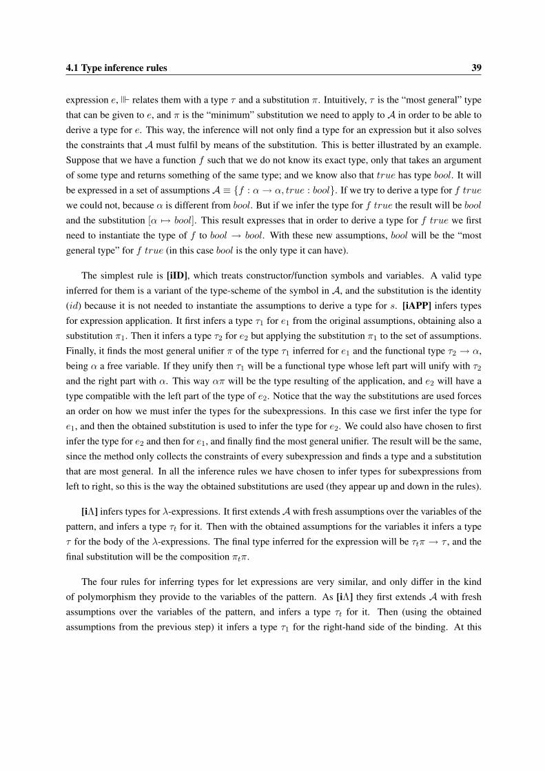
4.1 Type inference rules 39

expression e,� relates them with a type τ and a substitution π. Intuitively, τ is the “most general” type

that can be given to e, and π is the “minimum” substitution we need to apply to A in order to be able to

derive a type for e. This way, the inference will not only find a type for an expression but it also solves

the constraints that A must fulfil by means of the substitution. This is better illustrated by an example.

Suppose that we have a function f such that we do not know its exact type, only that takes an argument

of some type and returns something of the same type; and we know also that true has type bool. It will

be expressed in a set of assumptionsA ≡ {f : α→ α, true : bool}. If we try to derive a type for f true

we could not, because α is different from bool. But if we infer the type for f true the result will be bool

and the substitution [α 7→ bool]. This result expresses that in order to derive a type for f true we first

need to instantiate the type of f to bool → bool. With these new assumptions, bool will be the “most

general type” for f true (in this case bool is the only type it can have).

The simplest rule is [iID], which treats constructor/function symbols and variables. A valid type

inferred for them is a variant of the type-scheme of the symbol in A, and the substitution is the identity

(id) because it is not needed to instantiate the assumptions to derive a type for s. [iAPP] infers types

for expression application. It first infers a type τ1 for e1 from the original assumptions, obtaining also a

substitution π1. Then it infers a type τ2 for e2 but applying the substitution π1 to the set of assumptions.

Finally, it finds the most general unifier π of the type τ1 inferred for e1 and the functional type τ2 → α,

being α a free variable. If they unify then τ1 will be a functional type whose left part will unify with τ2and the right part with α. This way απ will be the type resulting of the application, and e2 will have a

type compatible with the left part of the type of e2. Notice that the way the substitutions are used forces

an order on how we must infer the types for the subexpressions. In this case we first infer the type for

e1, and then the obtained substitution is used to infer the type for e2. We could also have chosen to first

infer the type for e2 and then for e1, and finally find the most general unifier. The result will be the same,

since the method only collects the constraints of every subexpression and finds a type and a substitution

that are most general. In all the inference rules we have chosen to infer types for subexpressions from

left to right, so this is the way the obtained substitutions are used (they appear up and down in the rules).

[iΛ] infers types for λ-expressions. It first extendsA with fresh assumptions over the variables of the

pattern, and infers a type τt for it. Then with the obtained assumptions for the variables it infers a type

τ for the body of the λ-expressions. The final type inferred for the expression will be τtπ → τ , and the

final substitution will be the composition πtπ.

The four rules for inferring types for let expressions are very similar, and only differ in the kind

of polymorphism they provide to the variables of the pattern. As [iΛ] they first extends A with fresh

assumptions over the variables of the pattern, and infers a type τt for it. Then (using the obtained

assumptions from the previous step) it infers a type τ1 for the right-hand side of the binding. At this

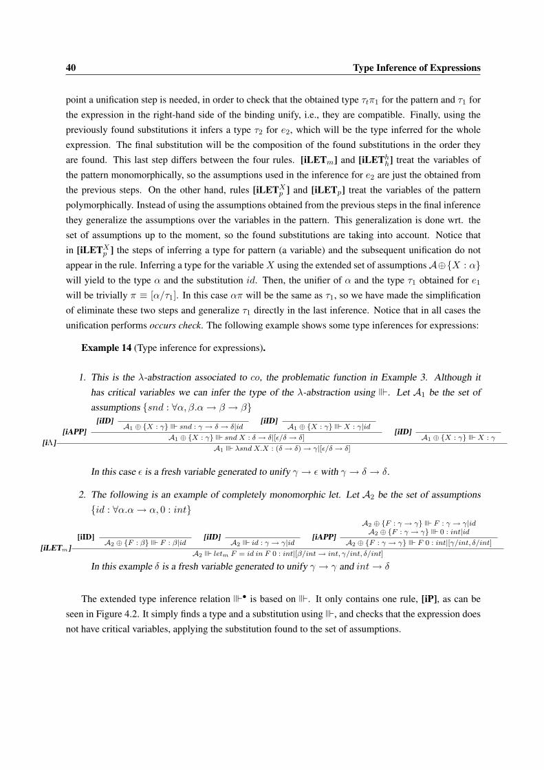
40 Type Inference of Expressions

point a unification step is needed, in order to check that the obtained type τtπ1 for the pattern and τ1 for

the expression in the right-hand side of the binding unify, i.e., they are compatible. Finally, using the

previously found substitutions it infers a type τ2 for e2, which will be the type inferred for the whole

expression. The final substitution will be the composition of the found substitutions in the order they

are found. This last step differs between the four rules. [iLETm] and [iLEThh] treat the variables of

the pattern monomorphically, so the assumptions used in the inference for e2 are just the obtained from

the previous steps. On the other hand, rules [iLETXp ] and [iLETp] treat the variables of the pattern

polymorphically. Instead of using the assumptions obtained from the previous steps in the final inference

they generalize the assumptions over the variables in the pattern. This generalization is done wrt. the

set of assumptions up to the moment, so the found substitutions are taking into account. Notice that

in [iLETXp ] the steps of inferring a type for pattern (a variable) and the subsequent unification do not

appear in the rule. Inferring a type for the variableX using the extended set of assumptionsA⊕{X : α}will yield to the type α and the substitution id. Then, the unifier of α and the type τ1 obtained for e1will be trivially π ≡ [α/τ1]. In this case απ will be the same as τ1, so we have made the simplification

of eliminate these two steps and generalize τ1 directly in the last inference. Notice that in all cases the

unification performs occurs check. The following example shows some type inferences for expressions:

Example 14 (Type inference for expressions).

1. This is the λ-abstraction associated to co, the problematic function in Example 3. Although it

has critical variables we can infer the type of the λ-abstraction using �. Let A1 be the set of

assumptions {snd : ∀α, β.α→ β → β}

[iΛ][iAPP]

[iID]A1 ⊕ {X : γ} � snd : γ → δ → δ|id

[iID]A1 ⊕ {X : γ} � X : γ|id

A1 ⊕ {X : γ} � snd X : δ → δ|[ε/δ → δ][iID]

A1 ⊕ {X : γ} � X : γ

A1 � λsnd X.X : (δ → δ)→ γ|[ε/δ → δ]

In this case ε is a fresh variable generated to unify γ → ε with γ → δ → δ.

2. The following is an example of completely monomorphic let. Let A2 be the set of assumptions

{id : ∀α.α→ α, 0 : int}

[iLETm][iID]

A2 ⊕ {F : β} � F : β|id[iID]

A2 � id : γ → γ|id[iAPP]

A2 ⊕ {F : γ → γ} � F : γ → γ|idA2 ⊕ {F : γ → γ} � 0 : int|id

A2 ⊕ {F : γ → γ} � F 0 : int|[γ/int, δ/int]A2 � letm F = id in F 0 : int|[β/int→ int, γ/int, δ/int]

In this example δ is a fresh variable generated to unify γ → γ and int→ δ

The extended type inference relation �• is based on �. It only contains one rule, [iP], as can be

seen in Figure 4.2. It simply finds a type and a substitution using�, and checks that the expression does

not have critical variables, applying the substitution found to the set of assumptions.

4.2 Type inference algorithm 41

It is usual in modern literature to split the inference process into two: the first step collects the

constraints between the types involved in the expression and the second solves them. This kind of

“Constraint-Based Typing” is explained in [58], where equality constraints are collected for the expres-

sions and solved with an unification algorithm. Others authors as [68] or [7] have gone further in this

topic, developing general frameworks where the constraint system is a paremeter. In this work we have

decided to keep the solving mechanism in the rules because the algorithm for finding most general uni-

fiers is well-known and is simple enough, and the whole inference process looks more compact.

4.2 Type inference algorithm

In the previous section we have presented inference as relations � and �•, which relates (A, e) with

(τ, π). But these relations can be viewed easily as recursive algorithms. Each rule (except [iID]) has the

same relation with subexpressions in the premises. And these premises in the rules of Figure 4.1 have a

clear order, due to the use of the obtained substitutions. The computation of variants in rule [iID] is easily

achieved by an algorithm, since it is just changing the quantified variables by fresh ones. And there exist

well-known algorithms for finding most general unifiers for syntactic unification, e.g. Robinson [63]

or Martelli-Montanari [46, 9]. Therefore the inference can be viewed as an algorithm that given (A, e)returns (τ, π), where each rule of the original relation expresses a different case and that fails if none of

the rules can be applied. This algorithm, called E after the famous algorithm W [48, 20, 19], appears in

Figure 4.3.

The situation is the same with relation �•. The relation � appears in its premises (a call to Ealgorithm), and it is also needed a checking of critical variables. The order between these two steps

is clear: we need first to find the substitution, and then use it to check the critical variables. By the

characterization of the opaque variables in Proposition 2 we can use �, i.e., algorithm E , to find the

opaque variables of a pattern. Then we can use the definition of critical variables (Definition 13) directly

as a recursive algorithm. The whole algorithm for inferring, called E•, can be found in Figure 4.2.

Notice that both algorithms E and E• are terminating. In the first case there are only recursive

calls where the the expression to infer types decreases strictly. In the base case, when the expression

is a symbol, the computation of a variant always finishes. The algorithm for finding the most general

unifiers is known to terminate, so the whole algorithm E is terminating. In the case of algorithm E• it

calls E , which is terminating, and also checks for critical variables. This checking terminates because

the recursive algorithm based on the definition is terminating (the argument decreases strictly), and the

computation of opaque variables that it uses also terminates (because it uses E). So the whole algorithm

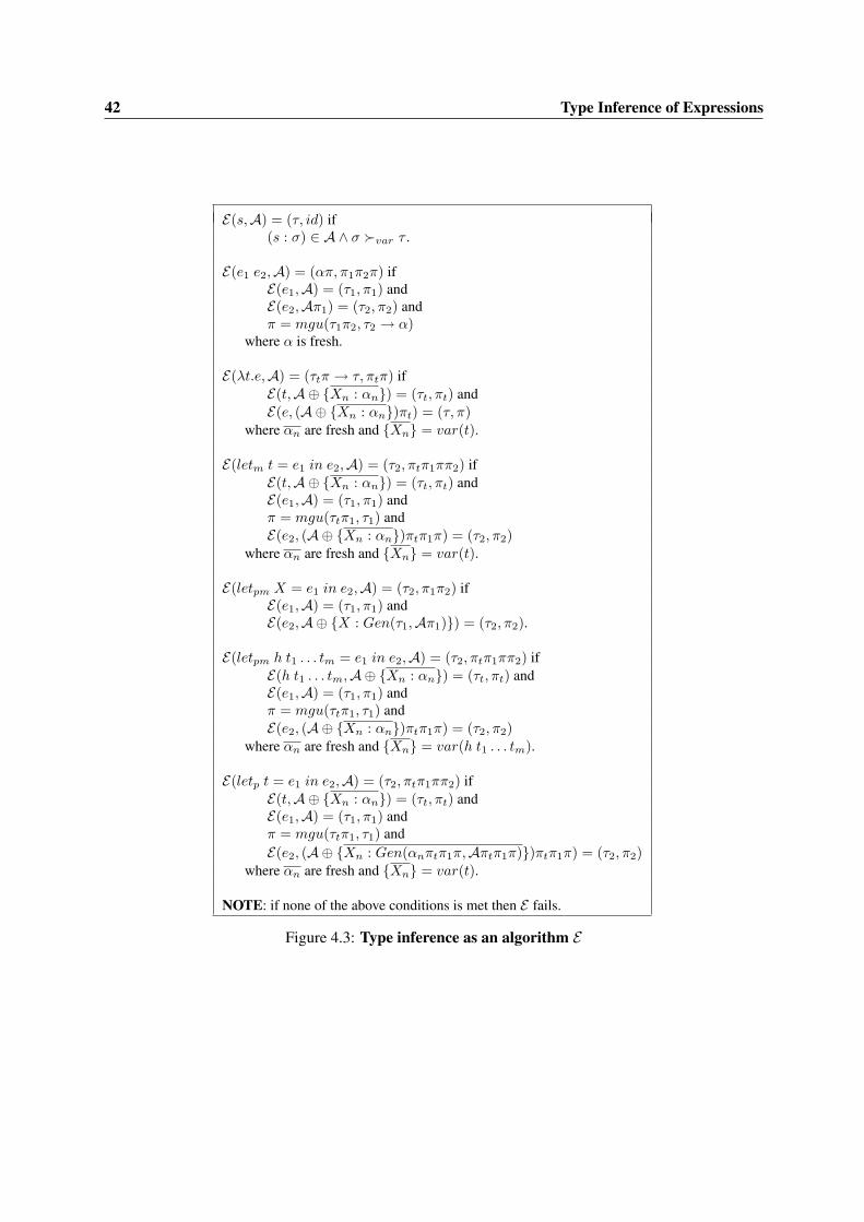
42 Type Inference of Expressions

E(s,A) = (τ, id) if(s : σ) ∈ A ∧ σ �var τ .

E(e1 e2,A) = (απ, π1π2π) ifE(e1,A) = (τ1, π1) andE(e2,Aπ1) = (τ2, π2) andπ = mgu(τ1π2, τ2 → α)

where α is fresh.

E(λt.e,A) = (τtπ → τ, πtπ) ifE(t,A⊕ {Xn : αn}) = (τt, πt) andE(e, (A⊕ {Xn : αn})πt) = (τ, π)

where αn are fresh and {Xn} = var(t).

E(letm t = e1 in e2,A) = (τ2, πtπ1ππ2) ifE(t,A⊕ {Xn : αn}) = (τt, πt) andE(e1,A) = (τ1, π1) andπ = mgu(τtπ1, τ1) andE(e2, (A⊕ {Xn : αn})πtπ1π) = (τ2, π2)

where αn are fresh and {Xn} = var(t).

E(letpm X = e1 in e2,A) = (τ2, π1π2) ifE(e1,A) = (τ1, π1) andE(e2,A⊕ {X : Gen(τ1,Aπ1)}) = (τ2, π2).

E(letpm h t1 . . . tm = e1 in e2,A) = (τ2, πtπ1ππ2) ifE(h t1 . . . tm,A⊕ {Xn : αn}) = (τt, πt) andE(e1,A) = (τ1, π1) andπ = mgu(τtπ1, τ1) andE(e2, (A⊕ {Xn : αn})πtπ1π) = (τ2, π2)

where αn are fresh and {Xn} = var(h t1 . . . tm).

E(letp t = e1 in e2,A) = (τ2, πtπ1ππ2) ifE(t,A⊕ {Xn : αn}) = (τt, πt) andE(e1,A) = (τ1, π1) andπ = mgu(τtπ1, τ1) andE(e2, (A⊕ {Xn : Gen(αnπtπ1π,Aπtπ1π)})πtπ1π) = (τ2, π2)

where αn are fresh and {Xn} = var(t).

NOTE: if none of the above conditions is met then E fails.

Figure 4.3: Type inference as an algorithm E

4.3 Properties of the type inference 43

E•(e,A) = (τ, π) ifE(e,A) = (τ, π) andcritV arAπ(e) = ∅.

NOTE: if none of the conditions is met then E• fails.

Figure 4.4: Extended type inference as an algorithm E•

E• is terminating as well.

4.3 Properties of the type inference

As we have said, inference is not only an effective way of finding some type for an expression. It has also

two important features: it recollects the “minimum” constraints that the set of assumptions must fulfil in

order to be able to derive any type for the expression (by means of the substitution) and it also finds the

most general type for the expression. In this section we will formalize these results.

The first important property of the inference is that the type found is a valid, i.e., there exists a type

derivation for that type using the set of assumptions affected by the substitution found. This result is

called the soundness of the inference, and it is stated in the next theorem. Here we will use the symbol

�? for any of the inference relations: � or�•.

Theorem 4 (Soundness of�?).A �? e : τ |π =⇒ Aπ `? e : τ

The substitution π found by the inference has the important property of being more general than any

other that permits to derive a type for the expression, i.e., they will be instances of π. The inferred type

has a similar property: if applying a substitution to the set of assumptions it is possible to derive a type,

the inferred type will be more general. The following theorem states this result for the inference relation

�.

Theorem 5 (Completeness of� wrt. `).If Aπ′ ` e : τ ′ then ∃τ, π, π′′. A � e : τ |π ∧ Aππ′′ = Aπ′ ∧ τπ′′ = τ ′.

If a derivation exists then the inference will succeed, finding a substitution and a type that are the

most general (upon renaming). Notice that this strong property is only valid with the relation�. A result

44 Type Inference of Expressions

similar to Theorem 5 cannot be obtained for �• because of critical variables, as the following example

shows.

Example 15 (Inexistence of a most general typing substitution).Let A be the set of assumptions {snd′ : α → bool → bool} and consider the following two valid

derivations

D1 : A[α/bool] ≡ {snd′ : bool→ bool→ bool} `• λ(snd′ X).X : (bool→ bool)→ bool

and

D2 : A[α/int] ≡ {snd′ : int→ bool→ bool} `• λ(snd′ X).X : (bool→ bool)→ int

It is clear that there is not a substitution more general than [α/bool] and [α/int] which makes possible a

type derivation for λ(snd′ X).X . The only substitution more general than these two will be [α/β] (for

some β), converting X in an opaque variable in snd′ X and thereby a critical variable in the expression.

In spite of this fact, we will see that�• is still able to find a most general substitution when it exists.

To formalize that, we will need the notion of the set collecting all type substitution π such that Aπ gives

some type to e.

Definition 16 (Typing substitutions of e).ΠeA = {π ∈ T Subst | ∃τ ∈ SType. Aπ ` e : τ}•ΠeA = {π ∈ T Subst | ∃τ ∈ SType. Aπ `• e : τ}

Now we are ready to formulate our result regarding the maximality of�•.

Theorem 6 (Maximality of�•).

a) •ΠeA has a maximum element⇐⇒ ∃τg ∈ SType, πg ∈ T Subst.A �• e : τg|πg.

b) If Aπ′ `• e : τ ′ and A �• e : τ |π then exists a type substitution π′′ such that Aπ′ = Aππ′′

and τ ′ = τπ′′.

The part a) of Theorem 6 states that if •ΠeA has a maximum element (wrt. the relation . between

substitutions) then the inference will succeed, and conversely, if the inference succeeds then the set •ΠeA

will have a maximum element. b) states that if there exists a type derivation Aπ′ `• e : τ ′ and the

type inference succeeds, then the substitution and the type found by the inference will be more general

than those appearing in the type derivation. Combining a) and b) we have that when there exists a most

4.3 Properties of the type inference 45

general substitution that allows to derive a type for an expression, the type inference will succeed and

will find it.

For finishing this chapter we will introduce a remark about the type inference that will be used in

the proofs of Appendix A. This observation shows that the result of the type inference is unique upon

renaming of fresh variables generated during the inference, so if they are replaced by other fresh variables

the result remains valid.

Remark 5 (Uniqueness of the type inference).The result of a type inference is unique upon renaming of fresh type variables. In a type inference

A � e : τ |π the variables in FTV (τ), Dom(π) or Rng(π) which do not occur in FTV (A) are fresh

variables generated by the inference process, so the result will remain valid if we change those variables

by any other fresh types variables.

Chapter 5

Type Inference of Programs

The type inference of a program is the method that, given a program (possibly with type declarations

for some functions), finds the types for the functions in the program and checks if the provided type

declarations are correct. In the previous chapter we presented type inference only for expressions. In

the functional programming setting, type inference does not need to distinguish between programs and

expressions, because the program can be incorporated in the expression by means of let expressions

and λ-abstractions. This way, the results given for expressions are also valid for programs. But in our

framework it is different, because our semantics (let-rewriting) does not support λ-abstractions and our

let expressions do not define new functions but only perform pattern matching. Thereby in our case we

cannot express a program as an expression, and we need to provide an explicit method for inferring the

types of a whole program. This explicit method is very important, as it is the core of the type stage in a

compiler.

In this chapter we will present two methods for inferring types for programs. Block inference (Section

5.2) infers types for a whole program “as is”. Stratified inference (Section 5.3) relies on the previous

one, but uses the dependencies between functions to split the program into blocks; which permits it to

infer types for more programs and/or need less type declarations. We will also introduce polymorphic

recursion, a situation which is not handled conveniently in the classical Damas & Milner type system.

48 Type Inference of Programs

5.1 Polymorphic recursion

Polymorphic recursion is the situation when different occurrences of the defined function appear with

different instances of the type of the function in its own recursive definition. This situation also arise

when dealing with a block of function definitions, which forces to handle them together. These situations

are illustrated in the following examples:

Example 16 (Inherent polymorphic recursion).data tree A = empty | node A (tree (tree A))

flatmap :: (A→ [B])→ [A]→ [B]

flatmap F [] = []

flatmap F (X:Xs) = (F X) ++ (flatmap F Xs)

collect Tree = case Tree of

empty→ []

node N T→ N : (flatmap collect (collect T))

This example has been extracted from [37]. It comes from the ML mailing list, and has arisen in

practice. Here tree A is a polymorphic tree type, and flatmap is a mapping function that also concatenates

the resulting lists. In this example collect is used with two types: tree (tree A) → [tree A] and

tree A → [A]. If polymorphic recursion is not allowed, this program will be rejected, since collect

should only have one type in the definition. It can be easily proved in GHC or Hugs. If we supply the

explicit type declaration for collect, ∀α.tree α→ [α], the program becomes typable.

Example 17 (Block of definitions with polymorphic recursion).map F L→ if (null L) then L else (F (head L)) : map F (tail L)

squarelist L→ map (λX.X ∗X) L

notlist L→ map not L

This example has been extracted from [50], and it only presents polymorphic recursion when the

three definitions are handled together. In this case, map is used with two different types: (int→ int)→[int] → [int] in squarelist and (bool → bool) → [bool] → [bool] in notlist. This block of definitions

will be correct if polymorphic recursion is supported, because both types are generic instances of the

type-scheme for map: ∀α, β.(α → β) → [α] → [β]. If polymorphic recursion is not supported this

block will be rejected, since map can only have type (int→ int)→ [int]→ [int] or (bool → bool)→[bool]→ [bool], but not both.

5.2 Block inference 49

Some other interesting examples needing polymorphic recursion can be found in [26], where the

authors compare their tipability with different type systems.

In the original Damas & Milner type system polymorphic recursion is not supported, because they

provide a FIX operator which forces the defined function and all its occurrences in the recursive def-

inition to have the same simple type. Mycroft [50] extends this type system by allowing polymorphic

recursion, providing a fix operator which lets the defined function and its occurrences to have the same

type-scheme. This way different occurrences could have different generic instances of them. [50] also ex-

tends the type inference to support polymorphic recursion, but the resulting algorithm is not terminating

in all cases. Later, [32, 39] proved (independently) that type inference in the presence of polymorphic

recursion is undecidable, due to it can be reduced to the problem of semiunification, which has been

proved to be semidecidable[38]. Therefore, any algorithm that tries to infer types in the presence of

polymorphic recursion can not terminate for certain cases. But if type-schemes are provided for the

polymorphic recursive functions the problem becomes decidable, since it is inferring types for the other

symbols and checking the provided type-schemes are correct.

5.2 Block inference

The type inference procedure for a program takes a set of assumptions A and a program P and returns a

type substitution π. The set A must contain assumptions for all the symbols in the program, even for the

functions defined in P . We want to reflect the fact that in practice some defined functions may come with

an explicit type declaration. Indeed this is a frequent way of documenting a program. Furthermore, type

declarations are sometimes a real need, as we have explained in the previous section about polymorphic

recursion. Therefore, for some of the functions –those for which we want to infer types– the assump-

tion will be simply a fresh type variable, to be instantiated by the inference process. For the rest, the

assumption will be a closed type-scheme, to be checked by the procedure. At the end, Aπ will contain

the assumptions for all the defined functions in the program.

Type inference of a program is defined as follows:

Definition 17 (Type Inference of a Program).The procedure B for type inference of a program {rule1, . . . , rulem} is defined as:

B(A, {rule1, . . . , rulem}) = π, if

1. A �• (ϕ(rule1), . . . , ϕ(rulem)) : (τ1, . . . , τm)|π.

50 Type Inference of Programs

2. Let f1 . . . fk be the function symbols of the rules rulei in P such that A(f i) is a closed type-

scheme, and τ i the type obtained for rulei in step 1. Then τ i must be a variant of A(f i).

ϕ is a transformation from rules to expressions defined as:

ϕ(f t1 . . . tn → e) = pair λt1. . . . λtn.e f

where () is the usual tuple constructor, with type () : ∀αi.α1 → . . . αm → (α1, . . . , αm); and pair is a

special constructor of tuples of two elements of the same type, with type pair : ∀α.α→ α→ α.

Procedure B first transforms the program into a single tuple expression, with as much elements as

rules in the program. Each rule is transformed into a special “pair” of elements of the same type, by

means of the transformation ϕ. The first element is the λ-abstraction associated to the rule, and the

second is the function symbol defined in the rule. This special “pair” forces the λ-abstraction and the

defined function symbol to have the same type if the inference succeed. The occurrence of the defined

function symbol in each pair also forces all the rules of the same function to have the same inferred type.

The absence of critical variables in the rules is guaranteed by the fact that the λ-abstractions appearing

in the expression have not critical variables. The second step checks that every defined functions with a

closed type-scheme in the assumptions (type declaration in the program), the inferred types for its rules

are variants of that type-scheme. If we did not perform this check the program would not be well-typed

wrt. Aπ, so the procedure would not be sound.

Notice that types inferred for the functions are simple types. In order to obtain type-schemes we need

and extra step of generalization, as discussed in Section 5.3.

5.2.1 Properties of block inference

The procedure B has two important properties. If B(A,P) finds a substitution π, then the program Pis well typed with respect to the assumptions Aπ. This soundness property is stated in the following

theorem.

Theorem 7 (Soundness of B).If B(A,P) = π then wtAπ(P).

Theorem 8 states the second property of B, called maximality. It states that if the procedure Bsucceeds, it finds a substitution that is more general than any other which makes the program well-typed.

5.3 Stratified inference 51

Theorem 8 (Maximality of B).If wtAπ′(P) and B(A,P) = π then ∃π′′ such that Aπ′ = Aππ′′.

It is not true in general that the existence of a well-typing substitution π′ implies the existence of a

most general one. Here we show a counterexample of this fact, which is very similar to that showed for

expressions in Example 15.

Example 18 (Inexistence of a most general well-typing substitution for a program).Let P be the program {snd X Y → Y, co (snd X) → X}, and let A be the set of assumptions

{snd : α → bool → bool, co : (bool → bool) → α}. The substitution π1 ≡ [α/bool] makes the

program well-typed, since Aπ1 `• λX.λY.Y : bool → bool → bool, which is a variant of Aπ1(snd) =bool → bool → bool; and Aπ1 `• λ(snd X).X : (bool → bool) → bool, which is a variant of

Aπ1(co) = (bool → bool) → bool. The program is also well-typed with π2 ≡ [α/int]. In both cases

the pattern snd X is not problematic because the substitutions eliminate the type variables of the type of

snd, so X is not opaque and therefore it is not critical.

The only substitution more general than π1 and π2 is π ≡ [α/β], being β any type variable. But this

substitution does not make the program well-typed, becauseAπ��̀•λ(sndX).X : (bool→ bool)→ β.

In this case X is opaque in snd X (since Aπ ⊕ {X : β} ` snd X : bool → bool and FTV (β) *FTV (bool→ bool)), and therefore it is critical.

5.3 Stratified inference

The procedure B handles programs has a block, without detecting the dependencies between functions.

This has the disadvantage of usually needing much explicit type declarations in order to succeed, be-

cause of polymorphic recursion. It is known that splitting a program into blocks of mutually dependent

functions and inferring the types in order may reduce the need of providing explicit type-schemes. This

situation is illustrated in the following example.

Example 19 (Block inference vs. stratified inference).Assume the block of definitions from Example 17:

map F L→ if (null L) then L else (F (head L)) : map F (tail L)

squarelist L→ map (λX.X ∗X) L

notlist L→ map not L

An attempt to apply the procedure B to infer types will fail, because it is not possible for map to

have types (int → int) → [int] → int and (bool → bool) → [bool] → bool at the same time. We

52 Type Inference of Programs

will need to provide explicitly the type-scheme for map : ∀α, β.(α → β) → [α] → [β] in order to the

type inference to succeed, yielding types squarelist : [int] → [int] and notlist : [bool] → [bool]. If

we examine the block, we discover that both squarelist and notlist depend on map, but map does not

depend on any other function in the block. Therefore we can split the block into three ordered blocks of

mutually dependent functions, where each block depends only on the previous ones:

P1 ≡ {map F L→ if (null L) then L else (F (head L)) : map F (tail L)}P2 ≡ {squarelist L→ map (λX.X ∗X) L} and

P3 ≡ {notlist L→ map not L}

If we infer types for P1 using B, we obtain for map the type (α → β) → [α] → [β], that is

completely generalized to ∀α, β.(α→ β)→ [α]→ [β]. With this assumption we can continue inferring

types for P2 and P3 and generalizing them, obtaining the expected types.

Definition 18 (Stratified inference).A general stratified inference procedure is defined in terms of the basic inference B in the following way:

1. Create the dependency graph of the program.

2. Calculate the graph of strongly connected components (SCCs) from the dependency graph.

3. Create blocks containing all the rules of the functions in the SCCs.

4. Sort the blocks according to any topological sort of the SCC graph.

5. For each block in the sorted list:

(a) Infer types with B using the the obtained types from the previous blocks.

(b) Generalize all the obtained types for the current block.

The dependency graph will contain as much vertices as defined functions in the program. In this

graph there will be an edge between f and g if g appears in the right-hand side or in any of the patterns

of the left-hand side in any rule of f . The computation of the SCC graph from the dependency graph is

easily achieved using any of the well-known algorithms that we will briefly discuss in next chapter. Each

strongly connected component will contain mutually dependent function. Since they are dependent their

types also depend on the other, so they must be inferred jointly. It is necessary to topologically sort the

SCCs in order to assure that we have all the type information that will be used while inferring types for a

block. Otherwise, we may need the type of a function that we have not inferred yet, or that has not been

checked (if we have an explicit type declaration).

5.3 Stratified inference 53

It is possible to simplify the generalization step 5b. We can assume that the original assumptions we

use to infer types for a program contains always closed-types schemes from the Prelude or other files, so

there will not be free type variables. After inferring types for each block using B, we generalize all type

variables appearing in them, without checking if the type variables occur free in the set of assumptions.

If they appear free they will only be in an assumption for a defined function in the same block (because

the rest are closed type-schemes), so the functions will be part of the same mutually dependent definition.

In this case we can safely generalize them, obtaining a closed set of assumptions again.

Notice that although stratified inference needs less explicit type-schemes, programs involving in-

herent polymorphic recursion still require explicit type-schemes in order to infer their types, as in the

program of Example 16.

Chapter 6

Implementation

In this chapter we will explain the most important issues about the implementation of the previously

defined algorithms of inference for expression/programs and stratified inference in Prolog [21, 66]. We

have chosen Prolog because this implementation will be part of the new version 3 of T OY , which will

be released soon. Since Prolog as been chosen as the main programming language in the development

of T OY 3, concretely Sicstus Prolog 4 [5], this implementation will fit easily. The vast majority of the

code follows the ISO Prolog Standard, making it easy to adapt from Sicstus 4 to any other Prolog system.

Indeed, it has been proved in SWI Prolog [73, 6], a free and popular Prolog system.

The current T OY compiler [69] does not check the absence of opaque patterns in the program, so it

accepts as valid programs like the polymorphic casting of Example 3. Apart from the detection of critical

variables, which solves the previous problem, our implementation contributes another improvement over

the existing type checking procedure in T OY: it allows programs with inherent polymorphic recursion

when suitable explicit types signatures are provided. Currently, the T OY compiler splits the program

into blocks of mutually dependent functions, as our stratified inference procedure. Then, it discards the

explicit type signatures provided by the programmer and infers types for the block. When it finishes, it

compares the inferred types to the user-defined types: if the inferred type for a function is more general, it

keeps the user-defined type (showing a warning message), otherwise it raises and error because the user-

defined type is more general than the inferred one. This way of performing the type inference prevents

the usage of explicit type signatures to allow polymorphic recursion, since the type inference is always

performed without using the user-defined types. Therefore, programs like the one in Example 16 are

rejected by the compiler, even when the explicit type for collect is provided. In our implementation the

program will be accepted when the explicit type ∀α.tree α → [α] is provided, and it will be rejected

56 Implementation

otherwise. Besides these improvements, our implementation also supports the three different kinds of

local declarations explained in this work. The existing T OY compiler only permits local definitions by

means of where declarations, which are treated in a completely monomorphic way1. Therefore, our

implementation provides more flexibility to the programmer in local declarations.

The code is divided in 4 files. operators.pl contains the definition of the operators used in the

syntax of expressions and types. infer.pl contains the predicates for inferring types of expressions

and programs. stronglycc.pl contains the implementation of Tarjan’s algorithm [70, 74] for find-

ing strongly connected components in graphs. Finally, stratified.pl contains the predicates for

inferring types for programs in the stratified way, using inference for expressions and programs and the

algorithm for the strongly connected component.

The complete code can be found in:

http://gpd.sip.ucm.es/enrique/systems/stratifiedInference/stratifiedInference.zip .

6.1 Syntax of the terms. Operators.

In the implementation, expressions, programs and types are represented as Prolog terms. In order to make

the syntax more readable, we have defined some infix operators. Data variables are represented as Prolog

variables, and constructor/function symbols as Prolog atoms. Expression application is represented as

Expr @ Expr, using the left associative infix operator @. λ-abstractions are terms constructed using

the functor lambda/2, where the first argument is the pattern and the second the expression. Let

expressions are represented using functors letm/2, letpm/2 and letp/2; where the first argument

is the pattern, the second the expression to bind and the third the expression of the body. Programs rules

are constructed with the functor rule/3 where the first argument is the function (an atom), the second

is the list of patterns of its left-hand side, and the third is the expression of the body. Finally, a program

is a Prolog list of program rules. The syntax of types in Prolog is summarized in the next figure.

Types need also be represented in the implementation (Figure 6.2). Type variables, like data vari-

ables, are represented by Prolog variables. This is very convenient since unification and occurs check is

handled automatically by the Prolog system, and no explicit handling of substitutions is required. Type

constructors are represented by common Prolog terms. For functional types we use the declared infix

operator -», which is right associative. Type application uses the same operator @ as expression applica-

tion. Type-schemes are represented using the functor tscheme/2, where the first argument is a list of

1since λ-lifting is used to eliminate where declarations.

6.1 Syntax of the terms. Operators. 57

Data variable 7→ Prolog variableConstructor/function symbol 7→ Prolog atom

Expression application 7→ Expr @ Exprλ-abstractions 7→ lambda(Pat,Expr)

Let expressions 7→ letm(Pat,Expr,Expr)| letpm(Pat,Expr,Expr)| letp(Pat,Expr,Expr)

Program rule 7→ rule(Func,ListOfPatterns,Body)Program 7→ Prolog list of program rules

Figure 6.1: Syntax of expressions and programs in Prolog

variables (those that are quantified) and the second is a simple type. An assumption is constructed using

the operator ::. This operator is infix and not associative. The left hand side is a variable or an atom

(data variable or constructor/function symbol) and the right-hand side is a simple type. Finally, sets of

assumptions are represented as lists of assumptions. In this implementation we also use facts of the form

type(Identifier,SimpleType) to store assumptions for constructors/function symbols due to

efficiency and simplicity. To infer types we need the types of all the symbols, in particular the types of

the built-in symbols, because they can appear elsewhere. If we only use a list of assumptions, every time

we need to find a variant of the type of a built-in symbol during the inference, we have to search in the

whole list, which is time consuming. But built-in symbols have always closed type-schemes, so they can

be stored easily in type/2 facts because free variables will not be a problem. This way, searching for

them is performed efficiently performed due to the indexing mechanism of the Prolog system. Moreover,

calculating a variant of a type stored in a type/2 fact is simpler and more efficient than a type stored in

a list of assumptions, as we will see in next section. Therefore, the list of assumptions will only contain

assumptions for variables and the symbols in the program, and the rest will be stored in type/2 facts.

Type variable 7→ Prolog variableType constructor 7→ Prolog atomFunctional type 7→ SimpleType1 -» SimpleType2

Type application 7→ SimpleType1 @ SimpleType2Type-scheme 7→ tscheme(VariableList, SimpleType)Assumption 7→ identifier :: TypeScheme

Set of assumptions 7→ Prolog list of assumptionsAssumption fact 7→ type(Identifier,SimpleType)

Figure 6.2: Syntax of types in Prolog

58 Implementation

6.2 Inference algorithms: infer.pl

This file contains the implementation of the inference algorithms E and E• for expressions and B for

programs. The most interesting predicates for expressions are:

• infer( +Assump, +Expr, -SimpleType )

It returns the inferred type for Expr using the set of assumptions Assump. The implementation

follows directly the pseudocode of Figure 4.3. In this case it is not necessary to handle substitutions

explicitly, because the Prolog system treats them automatically. We have included ad-hoc rules to

handle float and built-in types.

• inferp( +Assump, +Expr, -Type )

It implements the algorithm presented in Figure 4.4 using infer/3 and critVar/2.

• critVar( +Assump, +Expr ) This predicate checks that Expr has not any critical variable

wrt. Assump. It implements the alternative characterization of opaque variable of Proposition 2,

so it uses the infer/3 predicate.

• variant( +TScheme, -SimpleType )

This predicate takes a type-scheme tscheme( Gen, Type ) as an argument and returns a

simple type that is a variant. To create a variant we create a substitution (explicitly represented as

a list of pairs) from the generalized variables in Gen to fresh variables, and apply it to Type. It is

important this substitution by fresh variables, because if not different variants will share variables

as if they were free.

This predicate is only used with type-schemes stored in the list of assumptions. If the assumption is

stored in a fact, a call to type(Id,Type) will directly return a variant, since the Prolog system

will change the variables by fresh ones.

• gen( +Assump, +Type, -TypeScheme )

Returns the type-scheme resulting of the generalization of Type wrt. the set of assumptions

Assump. It looks in the free type variables of Assump (using ftv/2), and includes in the list of

generalized variables of TypeScheme those variables of Type not appearing in it.

• fv( +Expr, -EVars )

It returns a list of the free variables of the expression.

• ftv( +TypeScheme, -LVars ) / ftv( +Assump, -LVars )

It returns a list of the free variables of the type-scheme.

6.3 Strongly connected components algorithm: stronglycc.pl 59

For programs, the most interesting predicates are:

• b( ?Assump, +Prog )

Given a set of assumptions, infers the type of the function symbols defined in a program using

algorithm B (Definition 17). Notice that Assump is an input/output argument, so if b/2 succeeds

the assumptions for the symbols will have been instantiated to the proper types. If some symbols

in Assump contain a closed type-scheme as assumption, it will check that the inferred type is a

variant.

• b( +Assump, +Prog, +CheckList)

Previous predicate b/2 is defined in term of this. It act inferring types rule by rule. If it finds a

rule defining a function whose symbol has a type-scheme as an assumption, it adds the inferred

type to CheckList. When it finishes inferring type for the rules, processes the list to check that

the inferred types are variants of the type-schemes.

• check_variant( +Type, +Func, +Assump )

Checks that Type is a variant of the type-scheme stored in Assump for the function Func.

6.3 Strongly connected components algorithm: stronglycc.pl

This module implements Tarjan’s algorithm [70] for computing strongly connected components (SCCs)

of a graph. There exists more algorithms for computing SCCs, as Kosaraju’s [18] or Gabow’s [22]. A

complete explanation of the three algorithms and their code in C++ can be found in [64]. Kosaraju’s its

the classical algorithm for computing SCCs, its easy to implement and runs in O(|V |+ |E|) time when

the graph is represented adjacency lists, which is optimal because any algorithm for computing SCCs

must examine all the vertices (V) and edges (E). Kosaraju’s algorithm is based in the fact that the SCCs of

a graph and the transposed graph (the same vertices but changing the direction of the edges) are the same.

Although it is previous, Tarjan’s algorithm can be viewed as an improvement of Kosaraju’s. It runs also

in O(|V |+ |E|) time, but in practice it is more efficient than Kosaraju’s because it performs one depth-

first search on the graph instead of two. It is based on the fact that the SCCs form the subtrees of the

search tree, the roots of which are the roots of the SCCs. Gabow’s algorithm is the less known algorithm

of the three, and it also performs one depth-first search, but in practice its efficiency is comparable

with Tarjan’s, and its code is more complex. We have chosen Tarjan’s algorithm because of its balance

between efficiency and simplicity of code. The implementation of the algorithm has been based on the

pseudocode appearing in the Wikipedia [74], that we reproduce in Figure 6.3.

60 Implementation

1 I n p u t : Graph G = (V, E )

3 i n d e x = 0 / / DFS node number c o u n t e r4 S = empty / / An empty s t a c k o f nodes5 f o r a l l v in V do6 i f ( v . i n d e x i s u n d e f i n e d ) / / S t a r t a DFS a t each node7 t a r j a n ( v ) / / we haven ’ t v i s i t e d y e t

9 procedure t a r j a n ( v )10 v . i n d e x = i n d e x / / S e t t h e d e p t h i n d e x f o r v11 v . l o w l i n k = i n d e x12 i n d e x = i n d e x + 113 S . push ( v ) / / Push v on t h e s t a c k14 f o r a l l ( v , v ’ ) in E do / / C o n s i d e r s u c c e s s o r s o f v15 i f ( v ’ . i n d e x i s u n d e f i n e d ) / / Was s u c c e s s o r v ’ v i s i t e d ?16 t a r j a n ( v ’ ) / / Recur se17 v . l o w l i n k = min ( v . l o w l i n k , v ’ . l o w l i n k )18 e l i f ( v ’ i s in S ) / / Was s u c c e s s o r v ’ i n s t a c k S?19 v . l o w l i n k = min ( v . l o w l i n k , v ’ . i n d e x )20 i f ( v . l o w l i n k == v . i n d e x ) / / I s v t h e r o o t o f an SCC?21 p r i n t "SCC : "22 r ep ea t23 v ’ = S . pop24 p r i n t v ’25 u n t i l ( v ’ == v )

Figure 6.3: Pseudocode of Tarjan’s algorithm - Wikipedia [74]

6.4 Stratified inference: stratified.pl 61

We store the information of the edges of the graph using Prolog facts edge(A,B), which means

that there exists an edge between A and B (arrow from A to B). We also use a list containing the vertices

of the graph. This list is important because Tarjan’s algorithm only finds the SCCs of the vertices that are

reachable from the original vertex, so we need the list to call it from every unvisited vertex. Furthermore,

some vertices may not be involved in any edge, so they will not appear in any edge/2 fact. These

vertices will form a SCC by themselves. As they appear in the vertex list, they will be eventually used as

initial vertices for the algorithm, so the associated SCC will be handled correctly. We also need to store

persistent information about the vertices as their index (a number indicating the order of discovery) and

the lowest index of the vertices reachable from them. For efficiency reasons, we have chosen to store also

whether a node has been pushed in the stack instead of searching in the list. All this persisten information

is stored using dynamic predicates index(Node, Index), lowlink(Node, LowLink) and

instack(Node) that will be asserted and retracted during run-time.

The most important predicates of the file are:

• scc(+VertexList)The main predicate. It calculates the strongly connected components of the graph represented in

the edge/2 facts, and whose vertices appear in the list VertexList. The result is asserted as a

fact scc_list(SCC_List) containing the SCCs, each of them represented as a list of vertices.

• tarjan( +Vertex, +Index, +Stack, -NIndex, -NStack )

It calculates the SCCs of the graph starting from the vertex Vertex using Tarjan’s algorithm.

Index is the index counter, and Stack is the actual stack of vertices. It returns NIndex, the

new index counter; and NStack, the new stack of vertices. It uses the predicate findall/3 to

find the list of all the successor vertices of the current vertex.

• visit_successors( +Vertex, +SuccessorList, +Index, +Stack, -NewIndex,

-NewStack )

It visits all the vertices in SuccessorList which are the successors of the vertex Vertex.

This predicate implements the loop of the Tarjan’s algorithm that appears in lines 14-19 of Figure

6.3.

6.4 Stratified inference: stratified.pl

This file contains the implementation of the stratified inference for programs. This inference method

splits the whole program into sets of mutually dependent functions and infers the types set by set gener-

62 Implementation

alizing the obtained types, as explained in Section 5.3. The main predicate is stratified/1, whose

argument is the path of the file containing the program to infer types. The file contains a simple Prolog

program compound by type/2 and rule/3 facts. The syntax of this file is a simplification of a inter-

mediate representation of a source program containing only the relevant information for type inference.

type/2 facts act as type signatures in usual functional languages, and rule/3 facts represent function

rules as explained in Section 6.1.

The main predicates in this file are:

• stratified( +FileName )

It infers types for the program stored in FileName using the stratified method. It builds the

dependency graph, calculates the SCCs and infers type SCC by SCC. The inferred types are stored

in type/2 facts.

• retrieve_dependenciesIt captures the dependencies between functions from the rules and stores them using edge/2

facts, i.e., it builds the dependency graph from the rule/3 facts.

• inferSCC( +SCC )

It infers types for a SCC, storing the generalization of the inferred types using type/2 facts.

• genAssump( +Assump )

It generalizes the types appearing in Assump, adding them to the database using type/2 facts.

All the variables are generalized, even if they occur in Assump. Assump is assumed to contain

only {FunctionSymbol :: SimpleType} assumptions. This predicate is used by inferSCC/1

after inferring the types for a SCC using algorithm B.

• initialAssump( +SCC, -Assump )

It generates the initial assumptions for the functions in the list SCC. This predicate is used before

inferring types for a SCC. If the function F in Assump appears in a type(F,Type) fact, no

initial assumption is created. Otherwise, an assumption F::A (being A a new type variable) will

appear in Assump.

Chapter 7

Conclusions and Future Work

In this work we have presented a type system for functional logic languages that solves a well-known

problem which appears when HO patterns are handled naively in the type system. The results of this

work have been accepted as a paper in the 18th International Workshop on Functional and (Constraint)

Logic Programming (WFLP’09) held in Brasilia on June 28th. The paper has been also accepted to

appear in the Lecture Notes in Computer Science volume associated to the workshop.

7.1 Contributions of this work

• We have developed a type system based on Damas & Milner that solves the problems that ap-

pears due to opacity with HO patterns (Section 3.1.2). This type system is more flexible than the

proposed in [24], since it supports some HO patterns that the type system in [24] rejects. The

key resides in the notion of critical variables. In [24] they forbid any opaque pattern, whether it

contains opaque variables or not. In our type system we permit opaque patterns whenever they

do not contain critical variables, i.e., opaque variables which appear in the rest of the expression.

Therefore, a pattern like snd X which is rejected in [24] is allowed in our type system if the vari-

able X does not occur in the rest of the expression. We also allow opaque patterns without opaque

variables like snd true, which is rejected in [24] as well.

The uniform treatment of the opaque and critical variables allows us to be more liberal with the

types of data constructors, dropping the traditional restriction of transparency required to them.

Therefore data constructors can have non transparent types, and patterns containing them will be

accepted or rejected depending on the presence of critical variables, as in HO patterns.

64 Conclusions and Future Work

• We have clarified the different kinds of polymorphism that bound variables can have in let expres-

sions (Section 3.1.1). This is an issue that varies greatly between implementations of functional

and functional logic languages, and that is usually not documented nor formalized. We provide

a type system that supports three different kinds of polymorphism for let expressions explicitly,

without relying in any program transformation.

• The extension of the syntax of expressions in [24] with λ-abstractions and let expressions is other

of our contributions (Section 3.1.1). We have explicitly addressed the occurrence of compound

patterns in the arguments of λ-abstractions and in the bindings of let expressions, a fact usually

obviated in the literature or avoided by means of transformations. We provide a type system which

explicitly supports compound patterns.

• The type system developed has the subject reduction property (Section 3.3): expressions keep their

types after evaluation steps. This is a key property of type system, since it assures the absence of

type errors during run-time. For example, consider the boolean expression e1 ∧ true in which e1has type bool. We can be sure that after evaluation steps in e1 the resulting expression will have

type bool, so eventually we will be able to apply the rule for ∧1. This also assures that a well-

type expression will not lose its type during evaluation. In [24] they prove this property wrt. the

Goal-Oriented Rewriting Calculus (GORC). In this work we have proved subject reduction wrt.

let-rewriting [44], a small-step operational semantics for functional logic languages closer to real

computations.

• We have provided an inference algorithm for finding the type of expressions (Chapter 4). It is

stronger than a simple type-checker, since it also reconstructs the types of the symbols in the

expression when necessary. In the practice, this allows the programmer to omit the majority of the

type declarations in the program, as in languages like ML or Haskell. This algorithm is sound (the

types it finds are correct wrt. the type system) and “maximal” (it finds the most general type when

it exists). It cannot be complete because some expressions which admit type do not have a most

general one. In these cases the algorithm fails.

• We have also provided two explicit methods for inferring types for programs. In the functional

setting this is usually omitted because programs can be understood as chains of let expressions

defining functions accompanied by an expression to evaluate. In our framework this is not the

case, since our let expressions cannot define functions but perform pattern matching. These two

algorithms rely on the algorithm for inferring types for expressions. The block inference in Section

5.2 treats the program as a block. It has been proved to be sound (the program is well-typed with

the found types) and “maximal” (if it succeed it finds the most general types for the program). It is1if e1 is eventually evaluated to a pattern

7.2 Future work 65

not always possible to find the most general types because, as in the case of expressions, they do

not always exists. The stratified inference in Section 5.3 acts more cleverly, splitting the program

into mutually dependent components. This reduces the need of explicit type declarations.

• We have implemented the stratified inference in Prolog. It is an improvement over the existing

type inference procedure in the T OY compiler [69] because it detects critical variables and allows

polymorphic recursion when explicit types signatures are provided. It also supports the three

different kinds of local declarations (letm, letpm and letp), in contrast to the monomorphic where

declarations of the existing T OY system. Our implementation currently supports programs in a

very simplified format, but it will be soon extended and integrated in the T OY compiler as the

type stage. The source code of the stratified inference can be found in http://gpd.sip.ucm.es/

enrique/systems/stratifiedInference/stratifiedInference.zip .

• We have paid special attention to the formal aspects of the work. Therefore we have developed de-

tailed proofs of the properties of the type system, the subject reduction property, and the soundness

and completeness of the inference algorithms wrt. the type system. All the proofs can be found in

Appendix A.

7.2 Future work

In spite of the obtained results, there is still much work to do. Our first task is to integrate the stratified

inference into the T OY compiler. This will solve the problems that currently appear in the presence of

opaque HO patterns. To do that, it will be very useful the stratified inference for simplified programs

that we have already implemented in Prolog. Type errors management is a crucial issue in programming

systems, and it is not addressed in the current implementation. We plan to extend the implementation

with a robust type error management in order to produce informative errors to T OY users.

Other of our aims is to generalize the subject reduction property to let-narrowing [44], in order to

support the entire expressiveness of functional logic programming. Let-rewriting is a semantics with

call-time choice and nondeterministic functions, but it does not support the binding of variables during

execution, which is needed by programs as in Example 2. The generalization of the subject reduction

property to let-narrowing presents well-known problems [24, 8] like the instantation of higher order

variables, which is illustrated in the following example:

Example 20 (Binding of higher order variables).Let P be the program {add zero X → X, add (succ X) Y → succ(add X Y )}. If we have the

66 Conclusions and Future Work

expression F X == true, let-narrowing could find the substitution [F/add zero,X/true]. This is

a solution, since P ` add z true →l true, but clearly add z true is ill-typed. Let-narrowing finds

this substitution because it does not consider type information but only the program rules, so it cannot

perform any type checking while guessing instances. Therefore, let-narrowing needs to be extended to

support type information for programs and expressions.

We also want to handle extra variables (variables occurring only in the right-hand side of the rules),

a problem not investigated from the point of view of types. These variables may not have a type fixed

by the context where they appear, and it is not clear how much degree of polymorphism give to them in

such cases.

Our type system does not forbid opacity completely. It allows opaque variables when they do not

appear in the rest of the expressions, i.e., when they are not critical. This notion of opacity in expressions

is somehow similar to what happens with existential types [49] or generalized algebraic data types

[16, 61, 57], a connection that we plan to further investigate in the future. Finally, we are interested in

other known extensions of type system, like type classes [72, 52, 51] or generic programming [34, 35].

Bibliography

[1] Erlang programming language, official website. http://www.erlang.org.

[2] F# at microsoft research. http://research.microsoft.com/en-us/um/

cambridge/projects/fsharp/default.aspx.

[3] The glasgow haskell compiler. http://www.haskell.org/ghc/.

[4] The glorious glasgow haskell compilation system user’s guide, version 6.8.3; chapter 8: Ghc

language features; section 8.16. control over monomorphism. http://haskell.org/ghc/

docs/6.8.3/html/users_guide/monomorphism.html.

[5] Sicstus prolog homepage. http://www.sics.se/isl/sicstuswww/site/index.

html.

[6] Swi-prolog’s home. http://www.swi-prolog.org.

[7] ALVES, S., AND FLORIDO, M. Type inference using constraint handling rules. Electronic Notes

Theoretical Compututer Science 64 (2002).

[8] ANTOY, S., AND TOLMACH, A. P. Typed higher-order narrowing without higher-order strategies.

In Fuji International Symposium on Functional and Logic Programming (1999), pp. 335–353.

[9] BAADER, F., AND NIPKOW, T. Term Rewriting and All That. Cambridge University Press, 1998.

[10] BRASSEL, B. Two to three ways to write an unsafe type cast without importing unsafe - post to the

curry mailing list. http://www.informatik.uni-kiel.de/~curry/listarchive/

0705.html, May 2008.

[11] BRUS, T. H., VAN EEKELEN, C. J. D., VAN LEER, M. O., AND PLASMEIJER, M. J. Clean:

A language for functional graph rewriting. In Proc. of a conference on Functional programming

languages and computer architecture (London, UK, 1987), Springer-Verlag, pp. 364–384.

68 BIBLIOGRAPHY

[12] BUENO, F., CABEZA, D., CARRO, M., HERMENEGILDO, M., LÓPEZ, P., AND PUEBLA, G.

The Ciao Prolog System: A Next Generation Multi-Paradigm Programming Environment. REF-

ERENCE MANUAL, April 2006. Available at http://clip.dia.fi.upm.es/Software/

Ciao/ciao.pdf.

[13] CARDELLI, L. Type systems. In CRC Handbook of Computer Science and Engineering Handbook,

2nd ed. CRC Press, 2004, ch. 97.

[14] CARDELLI, L., AND WEGNER, P. On understanding types, data abstraction, and polymorphism.

ACM Computing Surveys 17 (1985), 471–522.

[15] CESARINI, F., AND THOMPSON, S. Erlang Programming. A Concurrent Approach to Software

Development. O’Reilly, 2009.

[16] CHENEY, J., AND HINZE, R. First-class phantom types. Tech. rep., Cornell University, July 2003.

[17] CLEMENT, D. The natural dynamic semantics of mini-standard ml. In II and Colloquium on Func-

tional and Logic Programming and Specifications (CFLP) on TAPSOFT ’87: Advanced Seminar

on Foundations of Innovative Software Development (New York, NY, USA, 1987), Springer-Verlag

New York, Inc., pp. 67–81.

[18] CORMEN, T. H., LEISERSON, C. E., RIVEST, R. L., AND STEIN, C. Introduction to Algorithms,

second ed. The MIT Press, 2001.

[19] DAMAS, L. Type Assignment in Programming Languages. PhD thesis, University of Edinburgh,

April 1985. Also appeared as Technical report CST-33-85.

[20] DAMAS, L., AND MILNER, R. Principal type-schemes for functional programs. In POPL ’82: Pro-

ceedings of the 9th ACM SIGPLAN-SIGACT symposium on Principles of programming languages

(New York, NY, USA, 1982), ACM, pp. 207–212.

[21] DERANSART, P., ED-DBALI, A., AND CERVONI, L. Prolog: The Standard. Reference Manual.

Springer, 1996.

[22] GABOW, H. N. Path-based depth-first search for strong and biconnected components. Inf. Process.

Lett. 74, 3-4 (2000), 107–114.

[23] GONZÁLEZ-MORENO, J., HORTALÁ-GONZÁLEZ, M., AND RODRÍGUEZ-ARTALEJO, M. A

higher order rewriting logic for functional logic programming. In Proc. International Conference

on Logic Programming (ICLP’97) (1997), MIT Press, pp. 153–167.

BIBLIOGRAPHY 69

[24] GONZÁLEZ-MORENO, J., HORTALÁ-GONZÁLEZ, T., AND RODRÍGUEZ-ARTALEJO, M. Poly-

morphic types in functional logic programming. In Journal of Functional and Logic Programming

(2001), vol. 2001/S01, pp. 1–71. Special issue of selected papers contributed to the International

Symposium on Functional and Logic Programming (FLOPS’99).

[25] GONZÁLEZ-MORENO, J. C., HORTALÁ-GONZÁLEZ, T., LÓPEZ-FRAGUAS, F., AND

RODRÍGUEZ-ARTALEJO, M. An approach to declarative programming based on a rewriting logic.

Journal of Logic Programming 40, 1 (1999), 47–87.

[26] HALLETT, J. J., AND KFOURY, A. J. Programming examples needing polymorphic recursion.

Tech. rep., Boston University, March 2004.

[27] HANUS, M. Functional logic programming. http://www.informatik.uni-kiel.de/

~mh/FLP/.

[28] HANUS, M. The integration of functions into logic programming: From theory to practice. Journal

of Logic Programming 19&20 (1994), 583–628.

[29] HANUS, M. Multi-paradigm declarative languages. In Proceedings of the International Conference

on Logic Programming (ICLP 2007) (2007), Springer LNCS 4670, pp. 45–75.

[30] HANUS (ED.), M. Curry: An integrated functional logic language (version 0.8.2). Available at

http://www.informatik.uni-kiel.de/~curry/report.html, March 2006.

[31] HARPER, R., MACQUEEN, D., AND MILNER, R. Standard ml. Lfcs report series ecs-lfcs-86-2,

University of Edinburgh, 1986.

[32] HENGLEIN, F. Type inference with polymorphic recursion. ACM Trans. Program. Lang. Syst. 15,

2 (1993), 253–289.

[33] HINDLEY, R. The principle type-scheme of an object in combinatory logic. Trans. Amer. Math.

Soc. 146 (1969), 29–60.

[34] HINZE, R. A new approach to generic functional programming. In POPL ’00: Proceedings of the

27th ACM SIGPLAN-SIGACT symposium on Principles of programming languages (New York,

NY, USA, 2000), ACM, pp. 119–132.

[35] HINZE, R. Generics for the masses. J. Funct. Program. 16, 4-5 (2006), 451–483.

[36] HUSSMANN, H. Non-Determinism in Algebraic Specifications and Algebraic Programs.

Birkhäuser Verlag, 1993.

70 BIBLIOGRAPHY

[37] JIM, T. What are principal typings and what are they good for? In POPL ’96: Proceedings of the

23rd ACM SIGPLAN-SIGACT symposium on Principles of programming languages (New York,

NY, USA, 1996), ACM, pp. 42–53.

[38] KFOURY, A. J., TIURYN, J., AND URZYCZYN, P. The undecidability of the semi-unification

problem. In STOC ’90: Proceedings of the twenty-second annual ACM symposium on Theory of

computing (New York, NY, USA, 1990), ACM, pp. 468–476.

[39] KFOURY, A. J., TIURYN, J., AND URZYCZYN, P. Type reconstruction in the presence of poly-

morphic recursion. ACM Trans. Program. Lang. Syst. 15, 2 (1993), 290–311.

[40] KFOURY, A. J., AND WELLS, J. B. Adding polymorphic abstraction to ml (detailed abstract),

1994.

[41] LEIJEN, D. HMF: Simple type inference for first-class polymorphism. In 13th ACM symp. of the

International Conference on Functional Programming (ICFP’08) (Sept. 2008). Extended version

available as Microsoft Research technical report MSR-TR-2007-118, Sep 2007.

[42] LEIJEN, D. Flexible types: robust type inference for first-class polymorphism. In POPL ’09:

Proceedings of the 36th annual ACM SIGPLAN-SIGACT symposium on Principles of programming

languages (New York, NY, USA, 2009), ACM, pp. 66–77. Extended version available as Microsoft

Research technical report MSR-TR-2008-55, Mar 2008.

[43] LLOYD, J. W. Programming in an integrated functional and logic language. Journal of Functional

and Logic Programming 3 (1999).

[44] LÓPEZ-FRAGUAS, F., RODRÍGUEZ-HORTALÁ, J., AND SÁNCHEZ-HERNÁNDEZ, J. Rewriting

and call-time choice: the HO case. In Proc. 9th International Symposium on Functional and Logic

Programming (FLOPS’08) (2008), vol. 4989 of LNCS, Springer, pp. 147–162.

[45] LÓPEZ-FRAGUAS, F., AND SÁNCHEZ-HERNÁNDEZ, J. T OY: A multiparadigm declarative sys-

tem. In Proc. Rewriting Techniques and Applications (RTA’99) (1999), Springer LNCS 1631,

pp. 244–247.

[46] MARTELLI, A., AND MONTANARI, U. An efficient unification algorithm. ACM Trans. Program.

Lang. Syst. 4, 2 (1982), 258–282.

[47] MCKINNA, J. Why dependent types matter. SIGPLAN Not. 41, 1 (2006), 1–1.

[48] MILNER, R. A theory of type polymorphism in programming. Journal of Computer and System

Sciences 17 (1978), 348–375.

BIBLIOGRAPHY 71

[49] MITCHELL, J. C., AND PLOTKIN, G. D. Abstract types have existential type. ACM Trans. Pro-

gram. Lang. Syst. 10, 3 (1988), 470–502.

[50] MYCROFT, A. Polymorphic type schemes and recursive definitions. In Proceedings of the 6th

Colloquium on International Symposium on Programming (London, UK, 1984), Springer-Verlag,

pp. 217–228.

[51] NIPKOW, T., AND PREHOFER, C. Type reconstruction for type classes. Journal of Functional

Programming 5, 2 (1995), 201–224.

[52] PETERSON, J., AND JONES, M. Implementing type classes. In PLDI ’93: Proceedings of the ACM

SIGPLAN 1993 conference on Programming language design and implementation (New York, NY,

USA, 1993), ACM, pp. 227–236.

[53] PEYTON JONES, S. The Implementation of Functional Programming Languages. Prentice Hall,

1987.

[54] PEYTON JONES, S., Ed. Haskell 98 Language and Libraries – The Revised Report. Cambridge

University Press, Cambridge, England, 2003.

[55] PEYTON JONES, S. Monomorphic pattern bindings - haskell prime wiki. http://hackage.

haskell.org/trac/haskell-prime/wiki/MonomorphicPatternBindings, July

2006.

[56] PEYTON JONES, S., VYTINIOTIS, D., WEIRICH, S., AND SHIELDS, M. Practical type inference

for arbitrary-rank types. J. Funct. Program. 17, 1 (2007), 1–82.

[57] PEYTON JONES, S., VYTINIOTIS, D., WEIRICH, S., AND WASHBURN, G. Simple unification-

based type inference for gadts. In ICFP ’06: Proceedings of the eleventh ACM SIGPLAN interna-

tional conference on Functional programming (New York, NY, USA, 2006), ACM, pp. 50–61.

[58] PIERCE, B. P. Types and programming languages. MIT Press, Cambridge, MA, USA, 2002.

[59] PIERCE, B. P. Advanced topics in types and programming languages. MIT Press, Cambridge, MA,

USA, 2005.

[60] PLASMEIJER, R., AND VAN EEKELEN, M. Clean version 2.1 Language Report, November 2002.

Available at http://clean.cs.ru.nl/contents/contents.html.

[61] POTTIER, F., AND RÉGIS-GIANAS, Y. Stratified type inference for generalized algebraic data

types. In POPL ’06: Conference record of the 33rd ACM SIGPLAN-SIGACT symposium on Prin-

ciples of programming languages (New York, NY, USA, 2006), ACM, pp. 232–244.

72 BIBLIOGRAPHY

[62] READE, C. Elements of Functional Programming. Addison-Wesley, 1989.

[63] ROBINSON, J. A. A machine-oriented logic based on the resolution principle. J. ACM 12, 1 (1965),

23–41.

[64] SEDGEWICK, R. Algorithms in C++, Part 5: Graph Algorithms. Addison-Wesley Professional,

2002, ch. 19.8. Strong Components in Digraphs, pp. 205–216.

[65] SOMOGYI, Z., HENDERSON, F. J., AND CONWAY, T. C. The execution algorithm of mercury, an

efficient purely declarative logic programming language. Journal of Logic Programming 29 (1996).

[66] STERLING, L., AND SHAPIRO, E. The Art of Prolog, second ed. The MIT Press, 1994.

[67] STRACHEY, C. Fundamental concepts in programming languages. Higher-Order and Symbolic

Computation 13, 1-2 (2000), 11–49.

[68] SULZMANN, M. F. A general framework for hindley/milner type systems with constraints. PhD

thesis, New Haven, CT, USA, 2000. Director-Hudak„ Paul.

[69] SÁNCHEZ, P. A., LEIVA, A. J. F., LUEZAS, A. G., FRAGUAS, F. J. L., ARTALEJO, M. R., AND

PÉREZ, F. S. TOY, A Multiparadigm Declarative Language. Version 2.3.1, 2007. Available at

http://toy.sourceforge.net/.

[70] TARJAN, R. Depth-first search and linear graph algorithms. SIAM Journal on Computing 1, 2

(1972), 146–160.

[71] TOFTE, M., AND TALPIN, J.-P. Region-based memory management. Inf. Comput. 132, 2 (1997),

109–176.

[72] WADLER, P., AND BLOTT, S. How to make ad-hoc polymorphism less ad hoc. In POPL ’89: Pro-

ceedings of the 16th ACM SIGPLAN-SIGACT symposium on Principles of programming languages

(New York, NY, USA, 1989), ACM, pp. 60–76.

[73] WIELEMAKER, J. An overview of the SWI-Prolog programming environment. In Proceedings

of the 13th International Workshop on Logic Programming Environments (Heverlee, Belgium, De-

cember 2003), F. Mesnard and A. Serebenik, Eds., Katholieke Universiteit Leuven, pp. 1–16. CW

371.

[74] WIKIPEDIA. Tarjan’s strongly connected components algorithm. http://en.wikipedia.

org/wiki/Tarjan%27s_strongly_connected_components_algorithm.

Appendix A

Proofs

A.1 Previous remarks and easy facts not formally proved

In this section we will present some remarks about the type system and the programs that will be used in

the proofs in the next section.

Remark 6.If A⊕ {Xn : τn} ` e : τ then we can assume that A⊕ {Xn : αn} � e : τ ′|π such that Aπ = A.

Explanation. Intuitively, the inference finds a type which is more general than all the possible types for

an expression, and also a type substitution which is necessary applying to the set of assumptions in order

to derive a type for the expression. In this case it is possible from the original set of assumptions A to

derive a type, so we do not need to changeA. Therefore the type substitution π from the inference would

not need to affect A, just only αn and the fresh variables generated during inference.

By Theorem 5 we know that there exists a type substitution π′′ such that Aππ′′ = A and τ ′π′′ = τ .

This means thatAπ is just a renaming of some free type variables ofA, which are restored with the type

substitution π′′. Being Aπ a renaming of A is a consequence of the mgu algorithm used. In this case,

during inference there will be some unifying steps between a free type variable α fromA and a fresh one

β. Clearly, both [α/β] and [β/α] are more general unifiers. In this cases if we choose the first, we will

compute a substitution which will make Aπ a renaming of A; but if we choose always to substitute the

fresh type variables the set of assumption Aπ will remain the same as A.

Remark 7.

74 Proofs

In a type derivation A ` e : τ will appear a type derivation for every subexpression e′ of e. That is, the

derivation will have a part of the tree rooted by A⊕ {Xn : τn} ` e′ : τ ′, being τ ′ a suitable type for e′,

and being {Xn : τn} a set of assumptions over variables of the expression e which have been introduced

by the rules [Λ], [LETm], [LETXpm], [LET hpm] or [LETp].If the expression is a pattern, the set of assumptions {Xn : τn} will be empty because the only rules used

to type a pattern are [ID] and [APP ].

Remark 8.If wtA(P) and A′ is a set of assumptions for variables, then wtA⊕A′(P).

The reason is that A′ does not change the assumptions for the function and constructor symbols in A.

Since there are not extra variables in the right hand sides, for every function rule in P the typing rule for

the lambda expression will add assumptions for all the variables, shadowing the provided ones.

A.2 Proofs of lemmas and theorems

In this section we will present the proofs of the lemmas and theorems in the work. We will also include

some auxiliary lemmas needed in the proofs of the main results.

The next lemma states that if we have a pattern t with type τ and we change its variables by other

expressions, the only way to obtain the same type τ for the substituted pattern is by changing the trans-

parent variables for expressions with the same type.

Lemma 1Assume A ⊕ {Xn : τn} ` t : τ , where var(t) ⊆ {Xn}. If A ` t[Xn/tn] : τ and Xj is a transparent

variable of t wrt. A then A ` tj : τj .

Proof. According to Observation 7, in the derivation of A ` t[Xn/tn] : τ appear derivations for every

subpattern ti, and they have the form A ` ti : τ ′i for some τ ′i . We will prove that if Xj is a particular

transparent variable of t, then τj = τ ′j . It is easy to see that taking the types τ ′n as assumptions for the

original variables Xn we can construct a derivation of A ⊕ {Xn : τ ′n} ` t : τ , simply replacing the

derivations for the subpatterns A ` ti : τ ′i with derivations for the variables A⊕ {Xn : τ ′n} ` Xi : τ ′i in

the original derivation for A ` t[Xn/sn] : τ . Since Xj is a transparent variable of t wrt A, by definition

A ⊕ {Xn : αn} � t : τg|πg and FTV (αjπg) ⊆ FTV (τg). By Theorem 5, if any type for t can be

derived from A⊕ {Xn : αn}πs then πg must be more general than πs. We know that there are (at least)

A.2 Proofs of lemmas and theorems 75

two substitutions π1 and π2 which can type t: π1 ≡ {αn 7→ τn} and π2 ≡ {αn 7→ τ ′n}, so they must

be more specific than πg (i.e. there exist π, π′ such that π1 = πgπ and π2 = πgπ′. We also know (by

Theorem 4) that A⊕ {Xn : αn} � t : τg|πg implies (A⊕ {Xn : αn})πg ` t : τg, and by Theorem 1-a

this implies that (A⊕ {Xn : αn})πgπ ` t : τgπ; so τgπ = τ (the same thing happens with π′: τgπ′ = τ

).

At this point we can distinguish two cases:

A) Xj is transparent because of FTV (αjπg) = ∅. Then τj = (αjπg)π = αjπg = (αjπg)π′ = τ ′j ,

because if αjπg does not have any free variable, it cannot be affected by any substitution.

B) Xj is transparent because of FTV (αjπg) ⊆ FTV (τg). As τgπ = τ and τgπ′ = τ , then for every

type variable β in FTV (τg) then βπ = βπ′. As every type variable β in FTV (αjπg) is also in

FTV (τg) then as τj = (αjπg)π = (αjπg)π′ = τ ′j .

The following lemma states that if the type inference of the expression e succeeds with Aπ, then the

type inference for the same expression will succeed with A. Besides, the types and substitutions found

will be related.

Lemma 2.If Aπ � e : τ1|π1 then ∃τ2 ∈ SType, π2 π

′′ ∈ T Subst s.t. A � e : τ2|π2 and τ2π′′ = τ1 and

Aπ2π′′ = Aππ1.

Proof. By Theorem 4A(ππ1) � e : τ1. Then applying Theorem 5A � e : τ2|π2 and there exists a type

substitution π′′ ∈ T Subst such that τ2π′′ = τ1 and Aπ2π′′ = Aππ1.

The following lemma states that if we have an expression e which can have a type τx, all the generic

instances of the type-scheme resulting of the generalization of that type are also valid types for the

expression e.

Lemma 3.If τ is a generic instance of Gen(τx,A) and A ` e : τx then A ` e : τ .

Proof. Let be Gen(τx,A) of the form ∀αi.τx according to the definition of generalization (Definition

11), being αi the type variables of τx which do not appear in A. By definition of generic instance

76 Proofs

(Definition 5) τ will have been constructed applying a type substitution π ≡ [αi/τi] to τx from the

variables αi to types, i.e., τ ≡ τxπ. BecauseA ` e : τx and the type system is closed under substitutions

(by Theorem 1-a) we can build a type derivation Aπ ` e : τxπ. But αi do not appear in A so Aπ ≡ Aand then A ` e : τ .

The lemma that follows states that the definition of opaque variables in Definition 12 and the more

operational characterization in Proposition 2 are equivalent.

Lemma 4 (Equivalence of the two characterizations of opaque variable).Let t be a pattern that admits type wrt. a given set of assumptions A. Then

∃τn, τ s.t. A⊕ {Xn : τn} ` t : τ and FTV (τi) * FTV (τ)⇐⇒

A⊕ {Xn : αn} � t : τg|πg and FTV (αiπg) * FTV (τg)

Proof.

=⇒ The type derivation can be written as (A ⊕ {Xn : αn})[αn/τn] ` t : τ , so by Theorem 5 A ⊕{Xn : αn} � t : τg|πg and there exists some π′′ ∈ T Subst s.t. τgπ′′ = τ , Aπgπ′′ = A and

αiπgπ′′ = τi. We only need to prove that

FTV (τi) * FTV (τ) =⇒ FTV (αiπg) * FTV (τg)

It is equivalent to prove

FTV (αiπg) ⊆ FTV (τg) =⇒ FTV (τi) ⊆ FTV (τ)

which is trivial since αiπgπ′′ = τi and τgπ′′ = τ , so

FTV (αiπg) ⊆ FTV (τg) =⇒ FTV (αiπgπ′′) ⊆ FTV (τgπ′′)

⇐= By Theorem 4 (A ⊕ {Xn : αn})πg ` t : τg, and FTV (αiπg) * FTV (τg). Since t admits type

by Observation 6 Aπg = A, so A⊕ {Xn : αnπg} ` t : τg.

The following is an important result that allow us to prove that type derivations `• are closed under

type substitutions. It states that if a pattern t has type with A and Aπ (for some assumptions for its

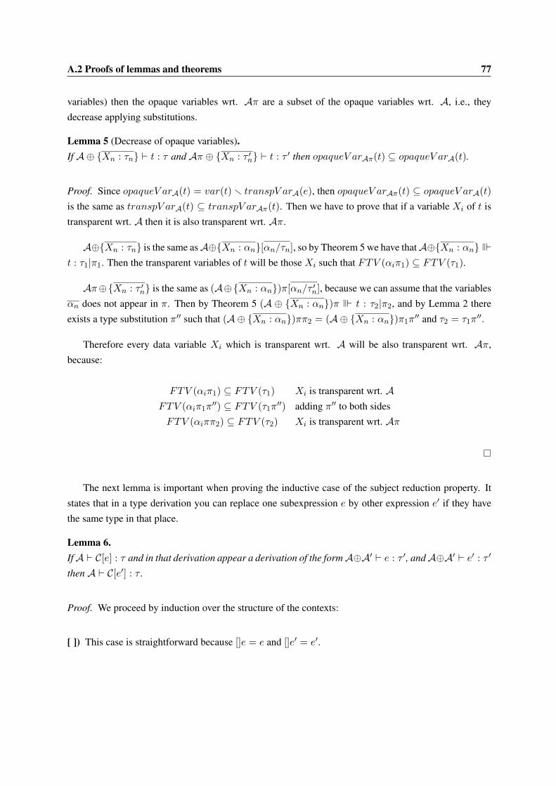
A.2 Proofs of lemmas and theorems 77

variables) then the opaque variables wrt. Aπ are a subset of the opaque variables wrt. A, i.e., they

decrease applying substitutions.

Lemma 5 (Decrease of opaque variables).If A⊕ {Xn : τn} ` t : τ and Aπ ⊕ {Xn : τ ′n} ` t : τ ′ then opaqueV arAπ(t) ⊆ opaqueV arA(t).

Proof. Since opaqueV arA(t) = var(t) r transpV arA(e), then opaqueV arAπ(t) ⊆ opaqueV arA(t)is the same as transpV arA(t) ⊆ transpV arAπ(t). Then we have to prove that if a variable Xi of t is

transparent wrt. A then it is also transparent wrt. Aπ.

A⊕{Xn : τn} is the same asA⊕{Xn : αn}[αn/τn], so by Theorem 5 we have thatA⊕{Xn : αn} �t : τ1|π1. Then the transparent variables of t will be those Xi such that FTV (αiπ1) ⊆ FTV (τ1).

Aπ⊕{Xn : τ ′n} is the same as (A⊕{Xn : αn})π[αn/τ ′n], because we can assume that the variables

αn does not appear in π. Then by Theorem 5 (A ⊕ {Xn : αn})π � t : τ2|π2, and by Lemma 2 there

exists a type substitution π′′ such that (A⊕ {Xn : αn})ππ2 = (A⊕ {Xn : αn})π1π′′ and τ2 = τ1π

′′.

Therefore every data variable Xi which is transparent wrt. A will be also transparent wrt. Aπ,

because:

FTV (αiπ1) ⊆ FTV (τ1) Xi is transparent wrt. AFTV (αiπ1π

′′) ⊆ FTV (τ1π′′) adding π′′ to both sides

FTV (αiππ2) ⊆ FTV (τ2) Xi is transparent wrt. Aπ

The next lemma is important when proving the inductive case of the subject reduction property. It

states that in a type derivation you can replace one subexpression e by other expression e′ if they have

the same type in that place.

Lemma 6.IfA ` C[e] : τ and in that derivation appear a derivation of the formA⊕A′ ` e : τ ′, andA⊕A′ ` e′ : τ ′

then A ` C[e′] : τ .

Proof. We proceed by induction over the structure of the contexts:

[ ]) This case is straightforward because []e = e and []e′ = e′.

78 Proofs

e1 C) Since (e1 C)[e] = e1 C[e], if we have a derivation for A ` (e1 C)[e] it must be of the form:

[APP]A ` e1 : τ1 → τ A ` C[e] : τ1

A ` e1 C[e] : τ

A derivation of A ⊕ A′ ` e : τ ′ must appear in the whole derivation, so it must appear in the

derivation A ` C[e] : τ1 (according to Observation 7). Since A ⊕ A′ ` e′ : τ ′ then by the

Induction Hypothesis we can state that A ` C[e′] : τ1, and we can construct a derivation for

A ` (e1 C)[e′]:

[APP]A ` e1 : τ1 → τ A ` C[e′] : τ1

A ` e1 C[e′] : τ

C e1) Similar to the previous case.

letm X = C in e1) (letm X = C in e1)[e] is equal to letm X = C[e] in e1, so a derivation of A `(letm X = C in e1)[e] : τ must have the form:

[LETm]A⊕ {X : τt} ` X : τt A ` C[e] : τt A⊕ {X : τt} ` e1 : τ

A ` letm X = C[e] in e1 : τ

Clearly, a derivation forA⊕A′ ` e : τ ′ will appear in the derivation forA ` C[e] : τt (Observation

7). Since A⊕A′ ` e′ : τ ′ then by the Induction Hypothesis we can state that A ` C[e′] : τt. With

this information we can construct a derivation for (letm X = C in e1)[e’]:

[LETm]A⊕ {X : τt} ` X : τt A ` C[e′] : τt A⊕ {X : τt} ` e1 : τ

A ` letm X = C[e′] in e1 : τ

letm X = e1 in C) A type derivation of (letm X = e1 in C)[e] will have the form:

[LETm]A⊕ {X : τt} ` X : τt A ` e1 : τt A⊕ {X : τt} ` C[e] : τ

A ` letm X = e1 in C[e] : τ

By Observation 7, the derivationA⊕{X : τt} ` C[e] : τ will contain a derivation (A⊕{X : τt})⊕A′′ ` e : τ ′. It is a premise that (A⊕ {X : τt})⊕A′′ ` e′ : τ ′ (in this case A′ = {X : τt} ⊕A′′),so by the Induction Hypothesis A ⊕ {X : τt} ` C[e′] : τ and we can construct a derivation

A ` letm X = e1 in C[e′] : τ

[LETm]A⊕ {X : τt} ` X : τt A ` e1 : τt A⊕ {X : τt} ` C[e′] : τ

A ` letm X = e1 in C[e′] : τ

rest) The proofs for the cases letpm X = C in e1, letpm X = e1 in C, letp X = C in e1 and

letp X = e1 in C are similar to the proofs for letm.

A.2 Proofs of lemmas and theorems 79

The lemma that follows states that in an expression e without critical variable, if you replace a

variable by any other expression which has not critical variables, the resulting expression has not critical

variables either.

Lemma 7.If critV arA(e) = ∅ and critV arA(e′) = ∅ then critV arA(e[X/e′]) = ∅.

Proof. We will proceed by induction over the structure of e.

Base Case

c) Straightforward because c[X/e′] = c, so critV arA(c[X/e′]) = critV arA(c) = ∅ from the

premises.

f ) The same as c.

X) In this case X[X/e′] = e′, and from the premises we know that critV arA(e′) = ∅.

Y ) Y is a variable distinct from X . Then Y [X/e′] = Y , and from the premises critV arA(Y ) = ∅.

Induction Step

e1 e2) By definition critV arA(e1 e2) = ∅ if critV arA(e1) = ∅ and critV arA(e2) = ∅. Then by

the Induction Hypothesis critV arA(e1[X/e′]) = ∅ and critV arA(e2[X/e′]) = ∅. By definition

(e1 e2)[X/e′] = e1[X/e′] e2[X/e′], so:

critV arA((e1 e2)[X/e′]) = critV arA(e1[X/e′] e2[X/e′])= critV arA(e1[X/e′]) ∪ critV arA(e2[X/e′])= ∅ ∪ ∅= ∅

λt.e) We assume that X /∈ var(t) and var(t) ∩ FV (e′) = ∅. Since critV arA(λt.e) = ∅ then

opaqueV arA(t)∩FV (e) = ∅ and critV arA(e) = ∅. opaqueV arA(t) ⊆ var(t), so opaqueV arA(t)∩

80 Proofs

FV (e′) = ∅. opaqueV arA(t)∩(FV (e)∪FV (e′)) = (opaqueV arA(t)∩FV (e))∪(opaqueV arA(t)∩FV (e′)) = ∅. Since FV (e[X/e′]) ⊆ FV (e)∪FV (e′), then opaqueV arA(t)∩FV (e[X/e′]) = ∅.

On the other hand by the Induction Hypothesis critV arA(e[X/e′]) = ∅. Therefore

critV arA((λt.e)[X/e′]) = critV arA(λt.(e[X/e′]))= (opaqueV arA(t) ∩ FV (e[X/e′])) ∪ critV arA(e[X/e′])= ∅ ∪ ∅= ∅

letm t = e1 in e2) We assume thatX /∈ var(t), var(t)∩FV (e′) = ∅, and var(t)∩FV (e1) = ∅. Since critV arA(letm t =e1 in e2) = ∅ then opaqueV arA(t) ∩ FV (e2) = ∅, critV arA(e1) = ∅ and critV arA(e2) = ∅.From var(t) ∩ FV (e′) = ∅ and opaqueV arA(t) ⊆ var(t) we know that opaqueV arA(t) ∩FV (e′) = ∅. As in the previous case, opaqueV arA(t)∩(FV (e2)∪FV (e′)) = ∅ andFV (e2[X/e′]) ⊆FV (e2) ∪ FV (e′), so opaqueV arA(t) ∩ FV (e2[X/e′]) = ∅.

On the other hand by the Induction Hypothesis critV arA(e1[X/e′]) = ∅ and critV arA(e2[X/e′]) =∅. Therefore

critV arA((letm t = e1 in e2)[X/e′]) = critV arA(letm t = e1[X/e′] in e2[X/e′])= (opaqueV arA(t) ∩ FV (e2[X/e′])) ∪

critV arA(e1[X/e′]) ∪ critV arA(e2[X/e′])= ∅ ∪ ∅ ∪ ∅= ∅

The proofs for the letpm and letp cases are equal to the letm case.

The next lemma states that if all fresh variables (wrt. a set of assumptions A) of a simple type τ do

not appear in a type substitution π, then generalizing τ wrt. A and applying π is the same as generalizing

the type with the substitution applied (τπ) wrt. the set of assumptions with the substitution applied (Aπ).

Lemma 8.Let A be a set of assumptions, τ a type and π ∈ T Subst such that for every type variable α which ap-

pears in τ and does not appear in FTV (A) then α /∈ Dom(π) and α /∈ Rng(π). Then (Gen(τ,A))π =Gen(τπ,Aπ).

Proof. We will study what happens with a type variable α of τ in both cases (types that are not variables

are not modified by the generalization step).

A.2 Proofs of lemmas and theorems 81

• α ∈ FTV (τ) and α ∈ FTV (A). In this case it cannot be generalized in Gen(τ,A), so in

(Gen(τ,A))π it will be transformed into απ. Because α ∈ FTV (A), then all the variables in

απ are in FTV (Aπ) and they cannot be generalized. Therefore in Gen(τπ,Aπ) α will also be

transformed into απ.

• α ∈ FTV (τ) and α /∈ FTV (A). In this case α will be generalized in Gen(τ,A), and as π does

not affect a generalized variable, it will remain in (Gen(τ,A))π. Because α is not in Dom(π),

then απ = α. α /∈ Rng(π) and α /∈ FTV (A), so it cannot appear in Aπ. Therefore α will also

be generalized in Gen(τπ,Aπ).

The following lemma states that the type that results of generalizing a simple type τ wrt. a set of

assumptions A and then applying a substitution π is always more general than the type that results of

generalizing τπ wrt. Aπ.

Lemma 9 (Generalization and substitutions).Gen(τ,A)π � Gen(τπ,Aπ)

Proof. It is clear that if a type variable α in τ is not generalized in Gen(τ,A) (because it occurs in

FTV (A)), then in the first type-scheme it will appear as απ. In the second type scheme it will also

appear as απ because all the variables in απ will be in Aπ (as α ∈ FTV (A.)). Therefore in every

generic instance of the two type-schemes this part will be the same. On the other hand, if a type variable

α is generalized in Gen(τ,A) then it will also appear generalized in Gen(τ,A)π (π will not affect it).

It does not matter what happens with this part απ in Gen(τπ,Aπ) because in every generic instance of

Gen(τ,A)π the generalized α will be able to adopt all the types of any generic instance of the part απ

in Gen(τπ,Aπ).

The lemma that follows shows an interesting property of the inference relation�. It states that if�•

succeeds with an expression e and a set of assumptions A then the sets of typing substitution ΠeA and

•ΠeA are the same. In other words, all type substitution that gives a type to e wrt. ` does not produce

critical variables and therefore it also gives a type to e wrt. `•.

Lemma 10.If A �• e : τ |π then Πe

A = •ΠeA.

82 Proofs

Proof. From definition of �• we know that A �• e : τ |π. We need to prove that ΠeA ⊆ •Πe

A and•ΠeA ⊆ Πe

A.

ΠeA ⊆ •Πe

A) We prove that π′ ∈ ΠeA =⇒ π′ ∈ •Πe

A. If π′ ∈ ΠeA then Aπ′ ` e : τ ′, and by Theorem 5 there

exists π′′ such that Aπ′ = Aππ′′ and τ ′ = τπ′′. By Theorem 4 Aπ `• e : τ , and by Theorem 1-a

Aππ′′ `• e : τπ′′, which is equal to Aπ′ `• e : τπ′′; so π′ ∈ •ΠeA .

•ΠeA ⊆ Πe

A) From definition of •ΠeA

The following is a very simple lemma that states that from a set of type derivations `• for expres-

sions en it is possible to create a type derivation `• for the tuple (en), and vice versa (where the tuple

constructor has the usual type ∀αn.α1 → . . . αn → (α1, . . . , αn)).

Lemma 11.A `• e1 : τ1, . . . ,A `• en : τn ⇐⇒ A `• (e1, . . . , en) : (τ1, . . . , τn)

Proof. Straightforward.

Lemma 12.A ` letm X = e2 in e1 X : τ ⇐⇒ A ` letp X = e2 in e1 X : τ , if X /∈ var(e1).

Proof. =⇒) In this case we have a type derivation

[LETm]A⊕ {X : τx} ` X : τx A ` e2 : τx

[APP]

A⊕ {X : τx} ` e1 : τx → τA⊕ {X : τx} ` X : τxA⊕ {X : τx} ` e1 X : τ

A ` letm X = e2 in e1 X : τ

It is clear that Gen(τx,A) � τx so A ⊕ {X : Gen(τx,A)} ` X : τx, and by Theorem 1-d

A⊕ {X : Gen(τx,A)} ` e1 : τx → τ . Therefore the following type derivation is valid:

[LETp]A⊕ {X : τx} ` X : τx A ` e2 : τx

[APP]

A⊕ {X : Gen(τx,A)} ` e1 : τx → τA⊕ {X : Gen(τx,A)} ` X : τxA⊕ {X : Gen(τx,A)} ` e1 X : τ

A ` letp X = e2 in e1 X : τ

A.2 Proofs of lemmas and theorems 83

⇐=) The type derivation is:

[LETp]A⊕ {X : τx} ` X : τx A ` e2 : τx

[APP]

A⊕ {X : Gen(τx,A)} ` e1 : τ ′ → τA⊕ {X : Gen(τx,A)} ` X : τ ′

A⊕ {X : Gen(τx,A)} ` e1 X : τA ` letp X = e2 in e1 X : τ

By Lemma 3 we know that A ` e2 : τ ′. Clearly A⊕ {X : τ ′} ` X : τ ′ is correct. As X does not

appear in e1 by Theorem 1-b the derivation A ⊕ {X : τ ′} ` e1 : τ ′ → τ is valid. Therefore we

can construct the following correct type derivation:

[LETm]A⊕ {X : τ ′} ` X : τ ′ A ` e2 : τ ′

[APP]

A⊕ {X : τ ′} ` e1 : τ ′ → τA⊕ {X : τ ′} ` X : τ ′

A⊕ {X : τ ′} ` e1 X : τA ` letp X = e2 in e1 X : τ

84 Proofs

The first theorem states some properties of the typing relations ` and `•. Part a) states the closure

under type substitutions. b) shows that type derivations for e depend only on the assumptions for the

symbols in e. c) is a substitution lemma stating that in a type derivation we can replace a variable by an

expression with the same type. Finally, d) establishes that from a valid type derivation we can change

the assumption of a symbol for a more general type-scheme, and we still have a correct type derivation

for the same type. Notice that this is not true wrt. the typing relation `• because a more general type can

introduce opacity.

Theorem 1 (Properties of the typing relations).

a) If A `? e : τ then Aπ `? e : τπ

b) Let s be a symbol not appearing in e. Then A `? e : τ ⇐⇒ A⊕ {s : σs} `? e : τ .

c) If A⊕ {X : τx} `? e : τ and A⊕ {X : τx} `? e′ : τx then A⊕ {X : τx} `? e[X/e′] : τ .

d) If A⊕ {s : σ} ` e : τ and σ′ � σ, then A⊕ {s : σ′} ` e : τ .

Proof.

a.1) If A ` e : τ then Aπ ` e : τπWe prove it by induction over the size of the type derivation of A ` e : τ .

Base Case

• [ID] If we have a derivation of A ` s : τ using [ID] is because τ is a generic instance of the

type-scheme A(g) = ∀αn.τ ′. We can change this type-scheme by other equivalent ∀βn.τ ′′ (ac-

cording to Observation 1) where each variable βi does not appear in Dom(π) nor in Rng(π).

Then the generic instance τ will be of the form τ ′′[βn/τn]. We need to prove that (τ ′′[βn/τn])π is

a generic instance of (∀βn.τ ′′)π. Since π does not involve any variable βi then (τ ′′[βn/τn])π =τ ′′π[βn/τnπ]. Applying a substitution to a type-scheme is (by definition) applying it only to its

free variables, but as no variable βi appears in π then (∀βn.τ ′′)π = ∀βn.(τ ′′π). Then it is clear

that τ ′′π[βn/τnπ] is a generic instance of (∀βn.τ ′′)π.

Induction Step

We have six different cases to consider accordingly to the inference rule used in the last step of the

derivation.

A.2 Proofs of lemmas and theorems 85

• [APP] In this case we have a derivation

[APP]A ` e1 : τ1 → τ A ` e2 : τ1

A ` e1 e2 : τ

By the Induction Hypothesis Aπ ` e1 : (τ1 → τ)π and Aπ ` e2 : τ1π. (τ1 → τ)π ≡ τ1π → τπ

so we can construct a derivation

[APP]Aπ ` e1 : τ1π → τπ Aπ ` e2 : τ1π

A ` e1 e2 : τπ

• [Λ] The derivation has the form

[Λ]A⊕ {Xn : τn} ` t : τt A⊕ {Xn : τn} ` e : τ

A ` λt.e : τt → τ

By the Induction Hypothesis (A⊕ {Xn : τn})π ` λt : τtπ and (A⊕ {Xn : τn})π ` e : τπ. But

(A⊕{Xn : τn})π ≡ Aπ⊕ ({Xn : τn})π ≡ Aπ⊕{Xn : τnπ} so we can build the type derivation

[Λ]Aπ ⊕ {Xn : τnπ} ` t : τtπ Aπ ⊕ {Xn : τnπ} ` e : τπ

Aπ ` λt.e : τt → τπ

• [LETm] The type derivation is

[LETm]A⊕ {Xn : τn} ` t : τt A ` e1 : τt A⊕ {Xn : τn} ` e2 : τ

A ` letm t = e1 in e2 : τ

By the Induction Hypothesis (A⊕{Xn : τn})π ` t : τtπ,Aπ ` e1 : τtπ and (A⊕{Xn : τn})π `e2 : τ . As in the previous case (A⊕ {Xn : τn})π ≡ Aπ ⊕ {Xn : τnπ}, so

[LETm]Aπ ⊕ {Xn : τnπ} ` t : τtπ Aπ ` e1 : τtπ Aπ ⊕ {Xn : τnπ} ` e2 : τπ

Aπ ` letm t = e1 in e2 : τπ

• [LETXpm] The derivation will be

[LETXpm]

A ` e1 : τx A⊕ {X : Gen(τx,A)} ` e2 : τ

A ` letXpm X = e1 in e2 : τ

First, we create a substitution π′ that maps the variables of τx which do not appear in FTV (A)to fresh variables which are not in FTV (A) and do not occur in Dom(π) nor in Rng(π). Then

by the Induction Hypothesis Aπ′ ` e1 : τxπ′. Since π′ does not contain in its domain any

variable in FTV (A), then Aπ′ = A and A ` e1 : τxπ′. π′ only substitutes variables which

do not appear in A by variables which are not in A either, so Gen(τx,A) = Gen(τxπ′,A).

Then A ⊕ {X : Gen(τxπ′,A)} ` e2 : τ is a valid derivation, and by the Induction Hypothesis

86 Proofs

(A ⊕ {X : Gen(τxπ′,A)})π ` e2 : τπ, which is the same that Aπ ⊕ {X : Gen(τxπ′,A)π} `e2 : τπ. By construction of π′ we know that for every variable of τxπ′ which does not appear

in A it will not be in Dom(π) nor in Rng(π). Then we can apply Lemma 8 and we have that

Aπ ⊕ {X : Gen(τxπ′π,Aπ)} ` e2 : τπ. By the Induction Hypothesis over A ` e1 : τxπ′ we

obtain Aπ ` e1 : τxπ′π. With this information we can construct a derivation

[LETXpm]

Aπ ` e1 : τxπ′π Aπ ⊕ {X : Gen(τxπ′π,Aπ)} ` e2 : τπ

Aπ ` letXpm X = e1 in e2 : τπ

• [LEThpm] Similar to the [LETm] case.

• [LETp] Similar to the [LETXpm] case, but instead of having to handle one single τx we need to

handle a set of τn. The main idea is the same, creating a substitution π′ to rename the variables

of the τn which do not appear in A and avoids their presence in the substitution π. Then we can

apply Lemma 8 to all the generalizations and proceed as in the [LETXpm] case.

a.2) If A `• e : τ then Aπ `• e : τπBy definition of `• we know that A ` e : τ and critV arA(e) = ∅. Then by Theorem 1-a Aπ ` e : τπ.

To prove that critV arAπ(e) = ∅ we use the decrease of opaque variables, stated in Lemma 5. FromA `e : τ and Aπ ` e : τπ we know that for every pattern t in e we have a derivation A⊕ {Xn : τn} ` t : τtandAπ⊕{Xn : τ ′n} ` t : τ ′, beingXn the data variables in t. Then we can prove that critV arAπ(e) = ∅by induction over the structure of e.

Base Case

s) critV arAπ(s) = ∅ by definition.

Induction Step

• e1e2) By the Induction Hypothesis we have that critV arAπ(e1) = ∅ and critV arAπ(e2) = ∅, so

critV arAπ(e1e2) = critV arAπ(e1) ∪ critV arAπ(e2) = ∅ ∪ ∅ = ∅.

• λt.e) By the Induction Hypothesis we have that critV arAπ(e) = ∅. critV arA(t) = ∅, so

(opaqueV arA(t)∩var(t)) = ∅. By Lemma 5 we know that opaqueV arAπ(t) ⊆ opaqueV arA(t),

A.2 Proofs of lemmas and theorems 87

so (opaqueV arAπ(t)∩var(t)) = ∅. Therefore critV arAπ(λt.e) = (opaqueV arAπ(t)∩var(t))∪critV arAπ(e) = ∅ ∪ ∅ = ∅.

• let∗ t = e1 in e2) Similar to the previous case.

b.1)Let be s a symbol which does not appear in e. Then A ` e : τ ⇐⇒ A⊕ {s : σs} ` e : τ .

=⇒) We will proceed by induction over the size of the derivation tree.

Base Case

[ID] In this case the derivation will be:

[ID] A ` s : τ

whereA(g) � τ . If we add an assumption over a symbol different from s then (A⊕{s : σs})(g) �τ , so

[ID]A⊕ {s : σs} ` s : τ

Induction Step

[APP] The derivation will have the form:

[APP]A ` e1 : τ ′ → τ A ` e2 : τ ′

A ` e1e2 : τ

By the Induction Hypothesis then A ⊕ {s : σs} ` e1 : τ ′ → τ and A ⊕ {s : σs} ` e2 : τ ′,therefore:

[APP]A⊕ {s : σs} ` e1 : τ ′ → τ A⊕ {s : σs} ` e2 : τ ′

A⊕ {s : σs} ` e1e2 : τ

[Λ] We have a type derivation

[Λ]A⊕ {Xn : τn} ` t : τ ′ A⊕ {Xn : τn} ` e : τ

A ` λt.e : τ ′ → τ

88 Proofs

By the Induction Hypothesis then (A⊕{Xn : τn})⊕{s : σs} ` t : τ ′ and (A⊕{Xn : τn})⊕{s :σs} ` e : τ . s does not appear in λt.e, so it will different from all the variables Xi and by

Observation 3 (A⊕ {Xn : τn})⊕ {s : σs} is the same as (A⊕ {s : σs})⊕ {Xn : τn}. Therefore

we can build a type derivation:

[Λ](A⊕ {s : σs})⊕ {Xn : τn} ` t : τ ′ (A⊕ {s : σs})⊕ {Xn : τn} ` e : τ

A⊕ {s : σs} ` λt.e : τ ′ → τ

[LETm] The type derivation will be:

[LETm]A⊕ {Xn : τn} ` t : τt A ` e1 : τt A⊕ {Xn : τn} ` e2 : τ

A ` letm t = e1 in e2 : τ

By the Induction Hypothesis then (A ⊕ {Xn : τn}) ⊕ {s : σs} ` t : τt, A ⊕ {s : σs} ` e1 : τtand (A⊕ {Xn : τn})⊕ {s : σs} ` e : τ . As in the previous case (A⊕ {Xn : τn})⊕ {s : σs} =(A⊕ {s : σs})⊕ {Xn : τn}, so we can build a type derivation:

[LETm]

(A⊕ {s : σs})⊕ {Xn : τn} ` t : τtA⊕ {s : σs} ` e1 : τt

(A⊕ {s : σs})⊕ {Xn : τn} ` e2 : τA⊕ {s : σs} ` letm t = e1 in e2 : τ

[LETXpm] The type derivation will be:

[LETXpm]

A ` e1 : τx A⊕ {X : Gen(τx,A)} ` e2 : τA ` letpm X = e1 in e2 : τ

Here the main problem is that Gen(τx,A) may not be same as Gen(τx,A⊕ {s : σs}). This

is caused because there are some type variables αn in FTV (τx) such that they appear free in

A but not in A ⊕ {s : σs} (they appear only in a previous assumption for s in A) or because

there are some type variables βn in FTV (τx) such that they do not occur free in A but they do

appear free in A ⊕ {s : σs} (they are added by σs). The first group of variables will be gen-

eralized in Gen(τx,A⊕ {s : σs}) but not in Gen(τx,A). To handle the second group we can

create a type substitution π from βn to fresh type variables. This way Gen(τxπ,A⊕ {s : σs})will be a type-scheme more general than Gen(τx,A), and by Theorem 1-d then A ⊕ {X :Gen(τxπ,A⊕ {s : σs})} ` e2 : τ . By Theorem 1-a we obtain the derivation Aπ ` e1 : τxπ,

and since βn are not in Dom(π) then A ` e1 : τxπ. By the Induction Hypothesis A ⊕ {s :σs} ` e1 : τxπ and (A ⊕ {X : Gen(τxπ,A⊕ {s : σs})}) ⊕ {s : σs} ` e2 : τ . As s is not in

letm X = e1 in e2 then it is different fromX , so (A⊕{X : Gen(τxπ,A⊕ {s : σs})})⊕{s : σs}is equal to (A⊕ {s : σs})⊕ {X : Gen(τxπ,A⊕ {s : σs})}.Therefore we can build the type derivation:

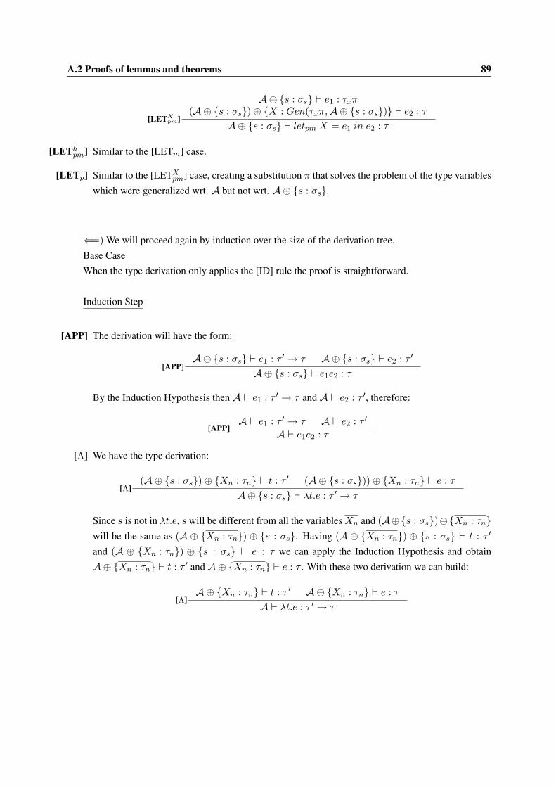
A.2 Proofs of lemmas and theorems 89

[LETXpm]

A⊕ {s : σs} ` e1 : τxπ(A⊕ {s : σs})⊕ {X : Gen(τxπ,A⊕ {s : σs})} ` e2 : τ

A⊕ {s : σs} ` letpm X = e1 in e2 : τ

[LEThpm] Similar to the [LETm] case.

[LETp] Similar to the [LETXpm] case, creating a substitution π that solves the problem of the type variables

which were generalized wrt. A but not wrt. A⊕ {s : σs}.

⇐=) We will proceed again by induction over the size of the derivation tree.

Base Case

When the type derivation only applies the [ID] rule the proof is straightforward.

Induction Step

[APP] The derivation will have the form:

[APP]A⊕ {s : σs} ` e1 : τ ′ → τ A⊕ {s : σs} ` e2 : τ ′

A⊕ {s : σs} ` e1e2 : τ

By the Induction Hypothesis then A ` e1 : τ ′ → τ and A ` e2 : τ ′, therefore:

[APP]A ` e1 : τ ′ → τ A ` e2 : τ ′

A ` e1e2 : τ

[Λ] We have the type derivation:

[Λ](A⊕ {s : σs})⊕ {Xn : τn} ` t : τ ′ (A⊕ {s : σs}))⊕ {Xn : τn} ` e : τ

A⊕ {s : σs} ` λt.e : τ ′ → τ

Since s is not in λt.e, s will be different from all the variables Xn and (A⊕{s : σs})⊕{Xn : τn}will be the same as (A ⊕ {Xn : τn}) ⊕ {s : σs}. Having (A ⊕ {Xn : τn}) ⊕ {s : σs} ` t : τ ′

and (A ⊕ {Xn : τn}) ⊕ {s : σs} ` e : τ we can apply the Induction Hypothesis and obtain

A⊕ {Xn : τn} ` t : τ ′ and A⊕ {Xn : τn} ` e : τ . With these two derivation we can build:

[Λ]A⊕ {Xn : τn} ` t : τ ′ A⊕ {Xn : τn} ` e : τ

A ` λt.e : τ ′ → τ

90 Proofs

[LETm] Similar to the [Λ] case.

[LETXpm] This case has to deal with the same problems as in [LETXpm] of the =⇒) case. We have a type

derivation:

[LETXpm]

A⊕ {s : σs} ` e1 : τx (A⊕ {s : σs})⊕ {X : Gen(τx,A⊕ {s : σs})} ` e2 : τA⊕ {s : σs} ` letpm X = e1 in e2 : τ

Again, the problem is that Gen(τx,A⊕ {s : σs}) may not be the same as Gen(τx,A). As before,

there may be variables αn in FTV (τx) which appear free in A ⊕ {s : σs} but not in A, and

variables βn in FTV (τx) which do not occur free in A ⊕ {s : σs} but they do appear free in

A. The first group is not problematic, because they are variables which will be generalized in

Gen(τx,A) but not in Gen(τx,A⊕ {s : σs}). To solve the problem with the second group we

create a type substitution π from β to fresh variables. This way Gen(τxπ,A) will be a more

general type-scheme than Gen(τx,A⊕ {s : σs}). Applying Theorem 1-d then (A⊕ {s : σs})⊕{X : Gen(τxπ,A)} ` e2 : τ . As s is different fromX , then (A⊕{s : σs})⊕{X : Gen(τxπ,A)}is the same as (A⊕{X : Gen(τxπ,A)})⊕{s : σs}, so the derivation (A⊕{X : Gen(τxπ,A)})⊕{s : σs} ` e2 : τ is correct. Applying the Induction Hypothesis to this derivation we obtain

A⊕{X : Gen(τxπ,A)} ` e2 : τ . By Theorem 1-a (A⊕{s : σs})π ` e1 : τxπ, which is equal to

A⊕ {s : σsπ} ` e1 : τxπ because βn do not occur free in A. Applying the Induction Hypothesis

to this derivation, we obtain A ` e1 : τxπ. Therefore we can build the type derivation:

[LETXpm]

A ` e1 : τxπ A⊕ {X : Gen(τxπ,A)} ` e2 : τA ` letpm X = e1 in e2 : τ

[LEThpm] Similar to the [Λ] case.

[LETp] Similar to the [LETXpm] case.

b.2) Let be s a symbol which does not appear in e, and σs any type. Then A `• e : τ ⇐⇒ A⊕ {s :σs} `• e : τ .

=⇒) By definition of A `• e : τ , A ` e : τ and critV arA(e) = ∅. Since s does not occur in e by

Theorem 1-b A ⊕ {s : σs} ` e : τ . It will also be true that critV arA⊕{s:σs}(e) = ∅ because the

opaque variables in the patterns will not change by adding the new assumption, and neither the

variables appearing in the rest of the expression. Therefore A⊕ {s : σs} `• e : τ .

A.2 Proofs of lemmas and theorems 91

⇐=) By definition of A⊕ {s : σs} `• e : τ , A⊕ {s : σs} ` e : τ and critV arA⊕{s:σs}(e) = ∅. s does

not appear in e, so by Theorem 1-b A ` e : τ . As in the previous case the critical variables of e

will not change by deleting an assumption which is not used, so A `• e : τ .

c.1) If A⊕ {X : τx} ` e : τ and A⊕ {X : τx} ` e′ : τx then A⊕ {X : τx} ` e[X/e′] : τ .

We will proceed by induction over the size of the expression e.

Base Case

[ID] If s 6= X then s[X/e′] ≡ s. On the contrary, if s = X then the derivation will be:

[ID]A⊕ {X : τx} ` X : τx

X[X/e′] ≡ e′, and the type derivation A⊕ {X : τx} ` e′ : τx comes from the hypothesis.

Induction Step

[APP] Just the application of the Induction Hypothesis.

[Λ] We can assume that λt.e is such that the variables Xn in its pattern do not appear inA⊕{X : τx}nor in FV (e′). The derivation will have the form:

[Λ](A⊕ {X : τx})⊕ {Xn : τn} ` t : τ ′ (A⊕ {X : τx})⊕ {Xn : τn} ` e : τ

A⊕ {X : τx} ` λt.e : τ ′ → τ

As X is different from Xn then (λt.e)[X/e′] ≡ λt.(e[X/e′]), so the first derivation remains the

same. We have from the hypothesis that A ⊕ {X : τx} ` e′ : τx. Since none of the Xn appear

in e′ then by Theorem 1-b we can add assumptions over that variables and obtain a derivation

(A⊕{X : τx})⊕{Xn : τn} ` e′ : τx. BecauseX 6= Xi for all i then by Observation 3 (A⊕{X :τx})⊕ {Xn : τn} is the same as (A⊕ {Xn : τn})⊕ {X : τx}. We have (A⊕ {Xn : τn})⊕ {X :τx} ` e : τ and (A⊕ {Xn : τn})⊕ {X : τx} ` e′ : τx, so applying the Induction Hypothesis we

obtain (A⊕ {Xn : τn})⊕ {X : τx} ` e[X/e′] : τ . Therefore we can build a new derivation:

92 Proofs

[Λ](A⊕ {X : τx})⊕ {Xn : τn} ` t : τ ′ (A⊕ {X : τx})⊕ {Xn : τn} ` e[X/e′] : τ

A⊕ {X : τx} ` λt.(e[X/e′]) : τ ′ → τ

[LETm] The proof is similar to the [Λ] case, provided that the variables of the pattern t do not occur in

FV (e′) nor in A⊕ {X : τx}.

[LETXpm] In this case Y is a fresh variable. The type derivation will be:

[LETXpm]

A⊕ {X : τx} ` e1 : τx (A⊕ {X : τx})⊕ {Y : Gen(τx,A⊕ {X : τx})} ` e2 : τA⊕ {X : τx} ` letpm Y = e1 in e2 : τ

By the Induction Hypothesis A ⊕ {X : τx} ` e1[X/e′] : τx. X 6= Y and Y /∈ FV (e′), soby Theorem 1-b we can add an assumption over the variable Y and get a derivation (A ⊕ {X :τx}) ⊕ {Y : Gen(τx,A⊕ {X : τx})} ` e′ : τx. By Observation 3 (A ⊕ {X : τx}) ⊕ {Y :Gen(τx,A⊕ {X : τx})} is equal to (A⊕ {Y : Gen(τx,A⊕ {X : τx})})⊕ {X : τx}, so by theInduction Hypothesis (A⊕ {Y : Gen(τx,A⊕ {X : τx})})⊕ {X : τx} ` e2[X/e′] : τ . Again byObservation 3 (A⊕{X : τx})⊕{Y : Gen(τx,A⊕ {X : τx})} ` e2[X/e′] : τ . Therefore we canconstruct a derivation:

[LETXpm]

A⊕ {X : τx} ` e1[X/e′] : τx (A⊕ {X : τx})⊕ {Y : Gen(τx,A⊕ {X : τx})} ` e2[X/e′] : τA⊕ {X : τx} ` letpm Y = e1[X/e′] in e2[X/e′] : τ

[LEThpm] Equal to the [LETm] case.

[LETp] The proof follows the same ideas as [LETm] and [LETXpm].

c.2) If A⊕ {X : τx} `• e : τ and A⊕ {X : τx} `• e′ : τx then A⊕ {X : τx} `• e[X/e′] : τ .

From the definition of `• we know that A ⊕ {X : τx} ` e : τ , A ⊕ {X : τx} ` e′ : τx,

critV arA⊕{X:τx}(e) = ∅ and critV arA⊕{X:τx}(e′) = ∅. Then by Theorem 1-c A ⊕ {X : τx} `

e[X/e′] : τ . By Lemma 7 we also know that critV arA⊕{X:τx}(e[X/e′]) = ∅, so by definition A⊕{X :

τx} `• e[X/e′] : τ .

A.2 Proofs of lemmas and theorems 93

d.1) If A⊕ {s : σ} ` e : τ and σ′ � σ, then A⊕ {s : σ′} ` e : τ .

Base Case

[ID] If e 6= s then is trivial. If e = s then the derivation will be:

[ID]A⊕ {s : σ} ` s : τ

where σ � τ . By Definition of generic instance, since σ′ � σ then σ′ � τ . So we can build the

derivation:

[ID]A⊕ {s : σ′} ` s : τ

Induction Step

[APP] We have a type derivation:

[APP]A⊕ {s : σ} ` e1 : τ ′ → τ A⊕ {s : σ} ` e2 : τ ′

A⊕ {s : σ} ` e1e2 : τ

By the Induction Hypothesis we have that A⊕ {s : σ′} ` e1 : τ ′ → τ and A⊕ {s : σ′} ` e2 : τ ′.Then we can construct a type derivation with the more general assumptions:

[APP]A⊕ {s : σ′} ` e1 : τ ′ → τ A⊕ {s : σ′} ` e2 : τ ′

A⊕ {s : σ′} ` e1e2 : τ

[Λ] We can assume that s is different from all the variables Xn. The type derivation will be:

[Λ](A⊕ {s : σ})⊕ {Xn : τn} ` t : τ ′ (A⊕ {s : σ})⊕ {Xn : τn} ` e : τ

A⊕ {s : σ} ` λt.e : τ ′ → τ

Since s is different from the variables Xn, then (A ⊕ {s : σ}) ⊕ {Xn : τn} is the same as (A ⊕{Xn : τn})⊕ {s : σ}. Therefore (A⊕ {Xn : τn})⊕ {s : σ} ` t : τ ′ and (A⊕ {Xn : τn})⊕ {s :σ} ` e : τ . By the Induction Hypothesis we have that (A ⊕ {Xn : τn}) ⊕ {s : σ′} ` t : τ ′ and

(A⊕{Xn : τn})⊕{s : σ′} ` e : τ ; and changing again the order in the assumptions we can build

a derivation:

[Λ](A⊕ {s : σ′})⊕ {Xn : τn} ` t : τ ′ (A⊕ {s : σ′})⊕ {Xn : τn} ` e : τ

A⊕ {s : σ′} ` λt.e : τ ′ → τ

[LETm] The proof is similar to the [Λ] case.

94 Proofs

[LETXpm] We assume that s 6= X . The type derivation is:

[LETXpm]

A⊕ {s : σ} ` e1 : τx (A⊕ {s : σ})⊕ {X : Gen(τx,A⊕ {s : σ})} ` e2 : τA⊕ {s : σ} ` letpm X = e1 in e2 : τ

By the Induction Hypothesis we have A ⊕ {s : σ′} ` e1 : τx. As σ′ � σ then by Observation 2

FTV (σ′) ⊆ FTV (σ). Therefore FTV (A⊕ {s : σ′}) = FTV (As)∪ FTV (σ′) ⊆ FTV (As)∪FTV (σ) = FTV (A⊕{s : σ}), beingAs the result of deleting fromA all the assumptions for the

symbol s. With this information it is clear that Gen(τx,A⊕ {s : σ′}) � Gen(τx,A⊕ {s : σ})because more variables could be generalized in Gen(τx,A⊕ {s : σ′}). Then by the Induction

Hypothesis (A⊕{s : σ})⊕{X : Gen(τx,A⊕ {s : σ′})} ` e2 : τ . As s 6= X then we can change

the order of the assumptions and obtain a derivation (A ⊕ {X : Gen(τx,A⊕ {s : σ′})}) ⊕ {s :σ} ` e2 : τ . Again by the Induction Hypothesis (A⊕{X : Gen(τx,A⊕ {s : σ′})})⊕{s : σ′} `e2 : τ . With these derivations we can build the one we were trying to construct:

[LETXpm]

A⊕ {s : σ′} ` e1 : τx (A⊕ {s : σ′})⊕ {X : Gen(τx,A⊕ {s : σ′})} ` e2 : τA⊕ {s : σ′} ` letpm X = e1 in e2 : τ

[LEThpm] Similar to the [Λ] case.

[LETp] The proof is similar to the [LETXpm] case.

The following theorem states that the transformation TRL(e) for eliminating compound patterns in

let expressions of Figure 3.4 preserves the type of the expression. It also states that the projection func-

tions created in the transformation are well-typed wrt. the original set of assumptions extended with the

assumptions for those functions.

Theorem 2 (Type preservation of the let transformation).Assume A `• e : τ and let P ≡ {fXn tn → Xn} be the rules of the projection functions needed in the

transformation of e according to Figure 3.4. Let also A′ be the set of assumptions over that functions,

defined as A′ ≡ {fXn : Gen(τXn ,A)}, where A �• λti.Xi : τXi |πXi . Then A ⊕ A′ `• TRL(e) : τand wtA⊕A′(P).

Proof. By structural induction over the expression e.

Base Case

A.2 Proofs of lemmas and theorems 95

• s) Straightforward.

Induction Step

• e1 e2) We have the type derivation:

[APP]

A ` e1 : τ1 → τA ` e2 : τ1A ` e1 e2 : τ

Let be A1 and A2 the assumptions over the projection functions needed in e1 and e2 respectively.

The by the Induction Hypothesis A ⊕ A1 ` TRL(e1) and A ⊕ A2 ` TRL(e2). Clearly the set

of assumptionsA′ over the projection functions needed in the whole expression isA1⊕A2. Then

by Theorem 1-b both derivations A ⊕ A′ ` TRL(e1) and A ⊕ A′ ` TRL(e2) are valid, and we

can construct the type derivation:

[APP]

A⊕A′ ` TRL(e1) : τ1 → τA⊕A′ ` TRL(e2) : τ1

A⊕A′ ` TRL(e1) TRL(e2) : τ

• letK X = e1 in e2) There are two cases, depending on the K:

letm X = e1 in e2:

The type derivation will be

[LETm]

A⊕ {X : τt} ` X : τtA ` e1 : τt

A⊕ {X : τt} ` e2 : τA ` letm X = e1 in e2 : τ

By the Induction Hypothesis A ` TRL(e1) : τt and A⊕ {X : τt} ` TRL(e2) : τ . Then we can

build the type derivation

[LETm]

A⊕ {X : τt} ` X : τtA ` TRL(e1) : τt

A⊕ {X : τt} ` TRL(e2) : τA ` letm X = TRL(e1) in TRL(e2) : τ

letp X = e1 in e2:

The type derivation for the original expression is

96 Proofs

[LETm]

A⊕ {X : τt} ` X : τtA ` e1 : τt

A⊕ {X : Gen(τt,A)} ` e2 : τA ` letp X = e1 in e2 : τ

By the Induction HypothesisA ` TRL(e1) : τt andA⊕{X : Gen(τt,A)} ` TRL(e2) : τ . Then

we can build the type derivation

[LETm]

A⊕ {X : τt} ` X : τtA ` TRL(e1) : τt

A⊕ {X : Gen(τt,A)} ` TRL(e2) : τA ` letp X = TRL(e1) in TRL(e2) : τ

• letpm X = e1 in e2) The type derivation for the original expression is

[LETpm]

A ` e1 : τtA⊕ {X : Gen(τt,A)} ` e2 : τA ` letpm X = e1 in e2 : τ

By the Induction Hypothesis A ` TRL(e1) : τt and A⊕ {X : Gen(τt,A)} ` TRL(e2) : τ . The

type derivation A⊕ {X : τt} ` X : τt is trivial, so we can build the type derivation

[LETm]

A⊕ {X : τt} ` X : τtA ` TRL(e1) : τt

A⊕ {X : Gen(τt,A)} ` TRL(e2) : τA ` letp X = TRL(e1) in TRL(e2) : τ

• letm t = e1 in e2) In this case the original type derivation is:

[LETm]

A⊕ {Xn : τn} ` t : τtA ` e1 : τt

A⊕ {Xn : τn} ` e2 : τA ` letm t = e1 in e2 : τ

It is easy to see that ifA⊕{Xn : τn} ` t : τt thenA ` λt.Xi : τt → τi. The assumptions over the

projections functions in A′ will be {fXn : Gen(τ ′t → τ ′n,A)}, where A � λt.Xi : τ ′t → τ ′i |πXi .

Since A ` λt.Xi : τt → τi we can assume that AπXi = A (Observation 6), and by Theorem 5 we

know that exists a type substitution π such that AπXiπ = Aπ = A and (τ ′t → τ ′i)π = τt → τi.

Therefore we can be sure that Gen(τ ′t → τ ′i ,A) � τt → τi, because π substitutes only the type

variables in τ ′t → τ ′i which are generalized inGen(τ ′t → τ ′i ,A). IfA′ contains all the assumptions

over the projection functions needed in the whole expression, it will contains assumptions over pro-

jection functions needed in e1 (A1), e2 (A2) and the pattern t (At ≡ {fXn : Gen(τ ′t → τ ′n,A)});so A′ = A1 ⊕A2 ⊕At. Then we can build the type derivation:

A.2 Proofs of lemmas and theorems 97

[LETm]A⊕A′ ⊕ {Y : τt} ` Y : τt A⊕A′ ` TRL(e1) : τt AY ` letm X1 = fX1 Y in . . . in TRL(e2) : τ

A⊕A′ ` letm Y = TRL(e1) in letm Xn = fXn Y in TRL(e2) : τ

where the derivation AY ` letm X1 = fX1 Y in . . . in TRL(e2) : τ is

[LETm]AY ⊕ {X1 : τ1} ` X1 : τ1

[APP]

AY ` fX1 : τt → τ1AY ` Y : τtAY ` fX1 Y : τ1 [LETm]

AY ⊕ {Xn : τn} ` TRL(e2) : τ. . .

AY ` letm X1 = fX1 Y in . . . in TRL(e2) : τ

(being AY ≡ A⊕A′ ⊕ {Y : τt}).

A ⊕ A′ ⊕ {Y : τt} ` Y : τt and AY ⊕ {X1 : τ1} ` X1 : τ1 are just the application of [ID]rule. By the Induction Hypothesis A ⊕ A1 ` TRL(e1) : τt, and by Theorem 1-b we can add the

assumptions A2 ⊕ At, obtaining A ⊕ A′ ` TRL(e1) : τt. AY ` fX1 Y : τ1 is straightforward

because Gen(τ ′t → τ ′i ,AπXi) � τt → τi for all the projection functions. It is easy to see that this

way the chain of let expressions will “collect” the same assumptions for the variables Xn that are

introduced by the pattern in the original expression: {Xn : τn}. Then by the Induction Hypothesis

A⊕{Xn : τn}⊕A2 ` TRL(e2) : τ , and by Theorem 1-b we can add the rest of the assumptions

and obtain A⊕ {Xn : τn} ⊕ A2 ⊕A1 ⊕At ⊕ {Y : τt} ` TRL(e2) : τ . Reorganizing the set of

assumptions (since the symbols are all different), we obtain AY ⊕ {Xn : τn} ` TRL(e2) : τ .

• letpm t = e1 in e2) This case is equal to the previous one because the derivation of the original

expression in both cases is the same (as t is a pattern we use [LEThpm], and this rule acts equal to

[LETm]) and the transformed expressions are the same.

• letp t = e1 in e2) The type derivation will be:

[LETp]

A⊕ {Xn : τn} ` t : τtA ` e1 : τt

A⊕ {Xn : Gen(τn,A)} ` e2 : τA ` letp t = e1 in e2 : τ

As in the previous case, A′ will be {fXn : Gen(τ ′t → τ ′n,AπXn)}, where A � λt.Xi : τ ′t →τ ′i |πXi . In addition, AπXi = A (Observation 6), Gen(τ ′t → τ ′i ,A) � τt → τi and A′ ≡ A1 ⊕A2 ⊕At. Then we can build a type derivation:

[LETp]A⊕A′ ⊕ {Y : τt} ` Y : τt A⊕A′ ` TRL(e1) : τt A′1 ` letm X1 = fX1 Y in . . . in TRL(e2) : τ

A⊕A′ ` letp Y = TRL(e1) in letp Xn = fXn Y in TRL(e2) : τ

98 Proofs

where the derivation AY ` letm X1 = fX1 Y in . . . in TRL(e2) : τ is

[LETp]A′1 ⊕ {X1 : τ1} ` X1 : τ1

[APP]

A′1 ` fX1 : τt → τ1A′1 ` Y : τtA′1 ` fX1 Y : τ1

[LETp][LETp]

A′n+1 ` TRL(e2) : τ. . .

A′2 ` letp X2 = fX2 Y in . . . in TRL(e2)

A′1 ` letp X1 = fX1 Y in . . . in TRL(e2) : τ

being A′1 ≡ A⊕A′ ⊕ {Y : Gen(τt,A⊕A′)} and A′i ≡ A′i−1 ⊕ {Xi−1 : Gen(τi−1,A′i−1)}.

As in the previous case, all the derivations A′i ` fXi Y : τi are valid, because A′i ` Y : τt. Notice

that Gen(τt,A) = Gen(τt,A⊕A′), as Observation 4 states, since FTV (A) = FTV (A ⊕ A′).

For the same reason, Gen(τi,A) = Gen(τi,A′i), so the chain of let expressions will collect the

same set of assumptions over the variablesXn: {Xn : Gen(τn,A)}. By the Induction Hypothesis,

we know that A ⊕ {Xn : Gen(τn,A)} ⊕ A2 ` TRL(e2) : τ ; and by Theorem 1-b we can

add the assumptions A1 ⊕ At ⊕ {Y : Gen(τt,A⊕A′) and obtain A ⊕ {Xn : Gen(τn,A)} ⊕A2 ⊕ A1 ⊕ At ⊕ {Y : Gen(τt,A⊕A′)} ` TRL(e2) : τ . Then reorganizing the assumptions

we obtain A ⊕ A′ ⊕ {Y : Gen(τt,A⊕A′)} ⊕ {Xn : Gen(τn,A)} ` TRL(e2) : τ . Since

Gen(τi,A) = Gen(τi,A′i) then the previous derivation is equal to A′n+1 ` TRL(e2) : τ .

In all the cases it is true that wtA⊕A′(P). Let Xi a data variable which is projected in the transformed

expression, and ti the compound pattern of a let expression where it appears. By Observation 7 we know

that in the derivation A `• e : τ will appear a derivation A ⊕ A′′ ⊕ {Xi : τ ′Xi} ` ti : τi for a set of

assumptions A′′ over some variables and Xi will not be opaque in ti wrt. A ⊕ A′′ ⊕ {Xi : τ ′Xi}. Then

it is clear that A ` λti.Xi : τi → τ ′Xi, and by Theorem 5 the type inference A � λti.Xi : τXi |πXi

will be correct. By Theorem 4 AπXi ` λti.Xi : τXi , and since by Observation 3 AπXi = A, then

A ` λti.Xi : τXi is a valid derivation. Clearly Xi is not opaque in ti wrt. A, because only the

assumptions for non variable symbols are used. Then critV arA(λti.Xi) = ∅, soA �• λti.Xi : τXi |πXi

and A `• λti.Xi : τXi . A′ contains assumptions over projection functions, and they do not appear in

λti.Xi, so by Theorem 1-b) we can add these assumptions and obtain A ⊕ A′ `• λti.Xi : τXi . We

know that in A′ there will appear an assumption {fXi : Gen(τXi ,A)} for the projection function of the

variable Xi, with rule fXi ti → Xi. We know that FTV (A) = FTV (A ⊕ A′) because since all the

assumptions in A are of the form Gen(τXi ,A) they will not add any type variable, and since no fXi

appears in A they will not shadow any assumption. Then τXi will be a variant of Gen(τXi ,A).

Therefore for every data variable Xi which is projected then A ` λti.Xi : τXi and τXi is a variant

of A⊕A′(fXi) = Gen(τXi ,A), so all the program rules fXi ti → Xi ∈ P ′ are well-typed wrt. A⊕A′

and wtA⊕A′(P ′).

A.2 Proofs of lemmas and theorems 99

The next theorem is one of the most important results of this work. It states that after a let-

rewriting step using a well-typed program, the resulting expression has the same type as the original

expression.

Theorem 3 (Subject Reduction).If A ` e : τ and wtA(P) and P ` e→l e′ then A ` e′ : τ .

Proof. We proceed by case distinction over the rule of the let-rewriting relation→l (Fig. 3.3) that we

use to reduce e to e′.

(Fapp) If we reduce an expression e using the (Fapp) rule is because e has the form f t1θ . . . tnθ (being

f t1 . . . tn → r a rule in P and θ ∈ PSubst) and e′ is rθ. In this case we want to prove that

A ` rθ : τ . Since wtA(P), then A `• λt1 . . . λtn.r : τ ′1 → . . . → τ ′n → τ ′, being τ ′1 → . . . →τ ′n → τ ′ a variant of A(f). We assume that the variables of the patterns tn do not appear in A or

in Rng(θ). The tree for this type derivation will be:

[Λ]A1 ` t1 : τ ′1

[Λ]A2 ` t2 : τ ′2

[Λ]

[Λ]An ` tn : τ ′n An ` r : τ ′

...A2 ` t3 . . . tn : τ ′3 → . . .→ τ ′n → τ ′

A1 ` λt2 . . . tn.r : τ ′2 → . . .→ τ ′n → τ ′

A ` λt1 . . . tn.r : τ ′1 → τ ′2 . . .→ τ ′n → τ ′

where Aj ≡ (. . . (A ⊕ {X1m : τ ′′1m}) ⊕ . . .) ⊕ {Xjm : τ ′′jm} and Xji is the i-th variable of the

pattern tj . We can write An as A ⊕ A′, being A′ the set of assumption over the variables of the

patterns. As these variables are all different (the left hand side of the rules is linear), by Theorem

1-b we can add the rest of the assumptions to the Aj to get An and the derivation will remain

valid, so ∀j ∈ [1, n].An ` tj : τ ′j . Besides critV arA(λt1 . . . λtn.r) = ∅, so a) every variable Xji

which appears in r is transparent in the pattern tj where it comes.

It is a premise that A ` f t1θ . . . tnθ : τ , and the tree of the type derivation will be:

[APP][APP]

[APP]

[APP][ID] A ` f : τ1 → . . .→ τn → τ A ` t1θ : τ1

...A ` f t1θ . . . tn−2θ : τn−1 → (τn → τ) A ` tn−1θ : τn−1

A ` f t1θ . . . tn−1θ : τn → τ A ` tnθ : τnA ` f t1θ . . . tnθ : τ

100 Proofs

Because of that, we know that b) ∀j ∈ [1, n].A ` tjθ : τj andA ` f : τ1 → . . .→ τn → τ , being

τ1 → . . .→ τn → τ a generic instance of the typeA(f). Then there will exists a type substitution

π such that (τ ′1 → . . . → τ ′n → τ ′)π = τ1 → . . . → τn → τ , so ∀j ∈ [1, n]. τ ′jπ = τj and

τ ′π = τ . What is more, Dom(π) does not contain any free type variable in A, since π transforms

a variant of the type of A(f) into a generic instance of the type of A(f). Then by Theorem 1-a

Anπ ` tj : τ ′jπ, which is equal to c) A⊕A′π ` tj : τ ′jπ.

With a), b) and c) and by Lemma 1 we can state that for every transparent variable Xji in r

then A ` Xjiθ : τ ′′jiπ. None of the variables in A′ appear in Xjiθ, so by Theorem 1-b we can

add these assumptions and obtain An ` Xjiθ : τ ′′jiπ. According to the first derivation, we have

An ` r : τ ′. Here we can apply the Theorem 1-a again and get a derivation Anπ ` r : τ ′π.

Because Anπ ` Xjiθ : τ ′′jiπ, then by Theorem 1-c Anπ ` rθ : τ ′π. As we have eliminated the

variables in the expression, by Theorem 1-b we can delete their assumptions, obtaining a derivation

Aπ ` rθ : τ ′π (remember thatAn isA⊕A′). And finally using the information we have about π,

this derivation is equal to A ` rθ : τ , the derivation we wanted to obtain.

(LetIn) In this case A ` e1e2 : τ and P ` e1e2 →l letm X = e2 in e1. The type derivation of e1e2 will

have the form:

[APP]A ` e1 : τ1 → τ A ` e2 : τ1

A ` e1e2 : τ

With this information we could build a type judgment for the letm expression

[LETm]A⊕ {X : τ1} ` X : τ1 A ` e2 : τ1

[APP]

A⊕ {X : τ1} ` e1 : τ1 → τA⊕ {X : τ1} ` X : τ1A⊕ {X : τ1} ` e1X : τ

A ` letm X = e2 in e1X : τ

A⊕ {X : τ1} ` X : τ1 is a valid derivation because is an application of the [ID] rule. And since

X is a fresh variable, by Theorem 1-b we can add the assumption and obtain A⊕ {X : τ1} ` e1 :τ1 → τ .

(Bind) We will distinguish between the letm and the letp case. In both cases we assume that the variable

X is fresh.

letm) In the letm case the type derivation will have the form:

[LETm]A⊕ {X : τt} ` X : τt A ` t : τt A⊕ {X : τt} ` e : τ

A ` letm X = t in e : τ

As X is different from all the variables Xn of the pattern t, then by Theorem 1-b we can add

the assumption over the variableX and obtain the derivationA⊕{X : τt} ` t : τt. Applying

A.2 Proofs of lemmas and theorems 101

the Theorem 1-c then A⊕ {X : τt} ` e[X/t] : τ . X will not appear in e[X/t], so again by

Theorem 1-b we can eliminate the assumption, concluding that A ` e[X/t] : τ .

letp) Here the type derivations will be:

[LETp]A⊕ {X : τt} ` X : τt A ` t : τt A⊕ {X : Gen(τt,A)} ` e : τ

A ` letp X = t in e : τ

and we want to prove that A ` e[X/t] : τ . We have a type derivation for A ⊕ {X :Gen(τt,A)} ` e : τ , and according to Observation 7 there will be derivations (A ⊕ {X :Gen(τt,A)}) ⊕ A′i ` X : τi for every appearance of X in e. In these cases, A′i will only

contain assumptions over variables Xn in let or lambda expressions of e. Suppose that all

these variables have been renamed to fresh variables. We can create a type substitution π

from the variables αn of τt which do not appear in A to fresh type variables βn. It is clear

that Gen(τt,A) is equivalent to Gen(τtπ,A), so A⊕ {X : Gen(τtπ,A)} ` e : τ is a valid

derivation. By Theorem 1-aAπ ` t : τtπ, and since αn are not inA thenA ` t : τtπ. X and

Xn are fresh so they do not appear in t and by Theorem 1-b we can add assumptions to the

derivation A ` t : τtπ, obtaining (A ⊕ {X : Gen(τtπ,A)}) ⊕ A′i ` t : τtπ. The types τnwill be generic instances ofGen(τt,A), and also ofGen(τtπ,A). Then for each τi there will

exist a type substitution π′i from the generalized variables βn inGen(τtπ,A) to types that will

hold τtππ′i ≡ τi. By Theorem 1-a we can convert (A⊕ {X : Gen(τtπ,A)})⊕A′i ` t : τtπinto ((A ⊕ {X : Gen(τtπ,A)}) ⊕ A′i)π′i ` t : τtππ′i, and as βn are fresh variables then

(A ⊕ {X : Gen(τtπ,A)}) ⊕ A′i ` t : τtππ′i (note that π′i does not affect Gen(τtπ,A)because the variables βn are generalized). This way in every place of the original derivation

where we have (A ⊕ {X : Gen(τt,A)}) ⊕ A′i ` X : τi we could place a derivation

(A ⊕ {X : Gen(τtπ,A)}) ⊕ A′i ` t : τi. The resulting expression of this substitution will

be e[X/t], so A ⊕ {X : Gen(τtπ,A)} ` e[X/t] : τ . It is clear that X does not appear

in e[X/t], so by Theorem 1-b we can eliminate the assumption over the X and obtain a

derivation A ` e[X/t] : τ , as we wanted to prove.

(Elim) In this case it does not matter what type of let expression it was (letm or letp). The rewriting step

will be of the form P ` let∗ X = e1 in e2 →l e2. The type derivation ofA ` let∗ X = e1 in e2 :τ will have a branch A ⊕ {X : σ′} ` e2 : τ for some σ. Since we are using the (Elim) rule, X

does not appear in e2 so by Theorem 1-b we can derive the same type eliminating that assumption,

obtaining A ` e2 : τ .

(Flatm) There are two cases, depending on the second let expression. In both cases we assume thatX 6= Y .

– P ` letm X = (letm Y = e1 in e2) in e3 →l letm Y = e1 in (letm X = e2 in e3).

102 Proofs

The type derivation will be:

[LETm]A⊕ {X : τx} ` X : τx

[LETm]

A⊕ {Y : τy} ` Y : τyA ` e1 : τy

A⊕ {Y : τy} ` e2 : τxA ` letm Y = e1 in e2 : τx A⊕ {X : τx} ` e3 : τ

A ` letm X = (letm Y = e1 in e2) in e3 : τ

Then we can build a type derivation

[LETm]A⊕ {Y : τy} ` Y : τy A ` e1 : τy

[LETm]

(A⊕ {Y : τy})⊕ {X : τx} ` X : τxA⊕ {Y : τy} ` e2 : τx

(A⊕ {Y : τy})⊕ {X : τx} ` e3 : τA⊕ {Y : τy} ` letm X = e2 in e3 : τ

A ` letm Y = e1 in (letm X = e2 in e3) : τ

The only two derivations which do not come from the hypotheses are (A⊕{Y : τy})⊕{X :τx} ` X : τx and (A ⊕ {Y : τy}) ⊕ {X : τx} ` e3 : τ . The first is the application of the

[ID] rule. From the hypotheses we have a derivation A ⊕ {X : τx} ` e3 : τ . Since we are

rewriting using the (Flat) rule, we are sure that Y is not in e3 and by Theorem 1-b we can

add the assumption over the Y , obtaining the derivation (A⊕{X : τx})⊕{Y : τy} ` e3 : τ .

X is different from Y , so according to Observation 3 (A⊕{X : τx})⊕{Y : τy} is the same

as (A ⊕ {Y : τy}) ⊕ {X : τx}. Therefore (A ⊕ {Y : τy}) ⊕ {X : τx} ` e3 : τ is a valid

derivation.

– P ` letm X = (letp Y = e1 in e2) in e3 →l letp Y = e1 in (letm X = e2 in e3). Similar

to the previous case.

(Flatp) We will treat the two different cases:

– P ` letp X = (letp Y = e1 in e2) in e3 →l letp Y = e1 in (letp X = e2 in e3).

The type derivation of the original expression is (being AY ≡ A⊕ {Y : Gen(τy,A)})

[LETp]A⊕ {X : τx} ` X : τx

[LETp]

A⊕ {Y : τy} ` Y : τyA ` e1 : τyAY ` e2 : τx

A ` letp Y = e1 in e2 : τx A⊕ {X : Gen(τx,A)} ` e3 : τA ` letp X = (letp Y = e1 in e2) in e3 : τ

A.2 Proofs of lemmas and theorems 103

With these derivations as hypothesis we can build a type derivation of the new expression

[LETp]A⊕ {Y : τy} ` Y : τy A ` e1 : τy

[LETp]

AY ⊕ {X : τx} ` X : τxAY ` e2 : τx

AY ⊕ {X : Gen(τx,AY )} ` e3 : τAY ` letp X = e2 in e3 : τ

A ` letp Y = e1 in (letp X = e2 in e3) : τ

A ⊕ {Y : τy} ` Y : τy, A ` e1 : τy and AY ` e2 : τx are the same derivations that

appear in the original type derivation; and AY ⊕ {X : τx} ` X : τx holds trivially applying

the [ID] rule. But the derivation AY ⊕ {X : Gen(τx,AY )} ` e3 : τ has to be proven.

As before, since Y /∈ FV (e3) by Theorem 1-b we can add an assumption over the Y and

the derivation (A ⊕ {X : Gen(τx,A)}) ⊕ {Y : Gen(τy,A)} ` e3 : τ will remain valid.

Because X 6= Y then by Observation 3 (A ⊕ {X : Gen(τx,A)}) ⊕ {Y : Gen(τy,A)} is

the same as (A ⊕ {Y : Gen(τy,A)}) ⊕ {X : Gen(τx,A)}, and the derivation (A ⊕ {Y :Gen(τy,A)}) ⊕ {X : Gen(τx,A)} ` e3 : τ will be correct. Clearly Gen(τx,AY ) is not

equal to Gen(τx,A) because a previous assumption for Y can be shadowed so that some

free type variables in A are not in AY . In the generalization step this means that some

variables can be generalized in Gen(τx,AY ) but not in Gen(τx,A). The other case never

happens because adding {Y : Gen(τy,A)} toA never adds free type variables: if some type

variable in τy is not in FTV (A) then it will be generalized and will not be in FTV (AY )either. ThereforeGen(τx,AY ) � Gen(τx,A), and by Theorem 1-d the derivation (A⊕{Y :Gen(τy,A)})⊕ {X : Gen(τx,AY )} ` e3 : τ is valid.

– P ` letp X = (letm Y = e1 in e2) in e3 →l letp Y = e1 in (letp X = e2 in e3).

The type derivation of the original expression is:

[LETp]A⊕ {X : τx} ` X : τx

[LETm]

A⊕ {Y : τy} ` Y : τyA ` e1 : τy

A⊕ {Y : τy} ` e2 : τxA ` letm Y = e1 in e2 : τx A⊕ {X : Gen(τx,A)} ` e3 : τ

A ` letp X = (letm Y = e1 in e2) in e3 : τ

and we want to build one of the form (being AY ≡ A⊕ {Y : Gen(τy,A)}):

[LETp]A⊕ {Y : τy} ` Y : τy A ` e1 : τy

[LETp]

AY ⊕ {X : τx} ` X : τxAY ` e2 : τx

AY ⊕ {X : Gen(τx,AY )} ` e3 : τAY ` letp X = e2 in e3 : τ

A ` letp Y = e1 in (letp X = e2 in e3) : τ

104 Proofs

The derivations A ⊕ {Y : τy} ` Y : τy and A ` e1 : τy come from the original derivation;

and AY ⊕ {X : τx} ` X : τx is the trivial application of the [ID] rule. From the original

derivation we have A ⊕ {Y : τy} ` e2 : τx. It is easy to see that Gen(τy,A) � τy,

so by Theorem 1-d AY ` e2 : τx. We also have from the original derivation that A ⊕{X : Gen(τx,A)} ` e3 : τ . We know that Y /∈ FV (e3), so by Theorem 1-b we can

add an assumption over that variable and the derivation (A ⊕ {X : Gen(τx,A)}) ⊕ {Y :Gen(τy,A)} ` e3 : τ will be valid. X is different from Y , so according to Observation 3

the set of assumptions (A ⊕ {X : Gen(τx,A)}) ⊕ {Y : Gen(τy,A)} is the same as (A ⊕{Y : Gen(τy,A)}) ⊕ {X : Gen(τx,A)}. By the same reasons given in the previous case

Gen(τx,AY ) � Gen(τx,A), so by Theorem 1-d the derivationAY ⊕{X : Gen(τx,AY )} `e3 : τ will be valid.

(LetAp) We will distinguish between the different let expressions.

letm) The rewriting step is P ` (letm X = e1 in e2)e3 →l letm X = e1 in e2e3. The type

derivation of (letm X = e1 in e2)e3 is:

[APP][LETm]

A⊕ {X : τt} ` X : τtA ` e1 : τt

A⊕ {X : τt} ` e2 : τ1 → τ

A ` letm X = e1 in e2 : τ1 → τ A ` e3 : τ1A ` (letm X = e1 in e2)e3 : τ

We want to construct a type derivation of the form:

[LETm]A⊕ {X : τt} ` X : τt A ` e1 : τt

[APP]

A⊕ {X : τt} ` e2 : τ1 → τA⊕ {X : τt} ` e3 : τ1A⊕ {X : τt} ` e2e3 : τ

A ` letm X = e1 in e2e3 : τ

All the derivations appear in the original derivation, except A⊕ {X : τt} ` e3 : τ1. Because

we are using (LetAp), we are sure that X does not appear in FV (e3). From the original

derivation we have that A ` e3 : τ1, and by Theorem 1-b we can add an assumption over the

variable X and obtain the derivation A⊕ {X : τt} ` e3 : τ1.

letp) Similar to the letm) case.

(Contx) We have a derivationA ` C[e] : τ , so according to the Observation 7 in that derivation will appear

a derivation a) A ⊕ A′ ` e : τ ′, being A′ a set of assumptions over variables. If we apply the

A.2 Proofs of lemmas and theorems 105

rule (Contx) to reduce an expression C[e] is because we reduce the expression e using any of the

other rules of the let-rewriting relation b) P ` e →l e′. We also know by Observation 8 that

c) wtA⊕A′(P). With a), b) and c) the Induction Hypothesis states that A ⊕ A′ ` e′ : τ ′, and by

Lemma 6 then A ` C[e′] : τ .

The next theorem states that� (resp. �•) is sound wrt. ` (resp. `•), i.e., that the type found by the

inference is a valid type for the expression applying the substitution to the set of assumptions.

Theorem 4 (Soundness of�?)1) A � e : τ |π =⇒ Aπ ` e : τ

Proof.

We proceed by induction over the size of the type inference A � e : τ |π.

Base Case

[iID] We have a type inference of the form:

[iID]A � g : τ |id

where A(g) = σ and τ is a variant of σ. It is clear that if τ is a variant of σ it is also a generic

instance of σ, and A id ≡ A so the following type derivation is valid:

[ID] A ` g : τ

Induction Step

[iAPP] The type inference is:

[iAPP]A � e1 : τ1|π1 Aπ1 � e2 : τ2|π2

A � e1e2 : απ|π1π2π

where π = mgu(τ1π2, τ2 → α), being α a fresh type variable. By the Induction Hypothesis we

have that Aπ1 ` e1 : τ1 and Aπ1π2 ` e2 : τ2. We can apply Theorem 1-a to both derivations and

obtainAπ1π2π ` e1 : τ1π2π andAπ1π2π ` e2 : τ2π. Since we know that τ1π2π = (τ2 → α)π =τ2π → απ then we can construct the type derivation:

106 Proofs

[APP]Aπ1π2π ` e1 : τ2π → απ Aπ1π2π ` e2 : τ2π

Aπ1π2π ` e1e2 : απ

[iΛ] The type inference will be of the form:

[iΛ]A⊕ {Xn : αn} � t : τt|πt (A⊕ {Xn : αn})πt � e : τ |π

A � λt.e : τtπ → τ |πtπ

where αn are fresh type variables. By the Induction Hypothesis we have thatAπt⊕{Xn : αnπt} `t : τt and Aπtπ ⊕ {Xn : αnπtπ} ` e : τ . We can apply Theorem 1-a to the first derivation and

obtain Aπtπ ⊕ {Xn : αnπtπ} ` t : τtπ. Therefore the following type derivation is correct:

[Λ]Aπtπ ⊕ {Xn : αnπtπ} ` t : τtπ Aπtπ ⊕ {Xn : αnπtπ} ` e : τ

Aπtπ ` λt.e : τtπ → τ

[iLETm] In this case the type inference will be:

[iLETm]

A⊕ {Xn : αn} � t : τt|πtAπt � e : τ1|π1

(A⊕ {Xn : αn})πtπ1π � e2 : τ2|π2

A � letm t = e1 in e2 : τ2|πtπ1ππ2

where αn are fresh type variables and π = mgu(τtπ1, τ1). By the Induction Hypothesis we have

that Aπt ⊕ {Xn : αnπt} ` t : τt, Aπtπ1 ` e : τ1 and Aπtπ1ππ2 ⊕ {Xn : αnπtπ1ππ2} ` e2 : τ2.

We can apply Theorem 1-a to the first two derivations and obtainAπtπ1ππ2⊕{Xn : αnπtπ1ππ2} `t : τtπ1ππ2 and Aπtπ1ππ2 ` e : τ1ππ2. Finally, as τtπ1π = τ1π then we can build a type deriva-

tion of the form:

[LETm]

Aπtπ1ππ2 ⊕ {Xn : αnπtπ1ππ2} ` t : τ1ππ2

Aπtπ1ππ2 ` e : τ1ππ2

Aπtπ1ππ2 ⊕ {Xn : αnπtπ1ππ2} ` e2 : τ2Aπtπ1ππ2 ` letm t = e1 in e2 : τ2

[iLETXpm] The inference will be:

[LETXpm]

A � e1 : τ1|π1 Aπ1 ⊕ {X : Gen(τ1,Aπ1)} � e2 : τ2|π2

A � letpm X = e1 in e2 : τ2|π1π2

By the Induction Hypothesis we have the type derivations Aπ1 ` e1 : τ1 and Aπ1π2 ⊕ {X :Gen(τ1,Aπ1)π2} ` e2 : τ2. We can construct a type substitution π ∈ T Subst such that maps the

type variables in FTV (τ1) rFTV (Aπ1) to fresh variables. Then it is clear that Gen(τ1,Aπ1) =Gen(τ1π,Aπ1). On the other hand, all the variables in τ1π which are not in FTV (Aπ1) are

fresh so they do not appear in π2, and by Lemma 8 Gen(τ1π,Aπ1)π2 = Gen(τ1ππ2,Aπ1π2).

A.2 Proofs of lemmas and theorems 107

Therefore the type derivation Aπ1π2 ⊕ {X : Gen(τ1ππ2,Aπ1π2)} ` e2 : τ2 is correct. By

Theorem 1-a we obtain Aπ1ππ2 ` e1 : τ1ππ2, and as Dom(π) ∩ FTV (Aπ1) = ∅ then Aπ1π2 `e1 : τ1ππ2.

Finally with these derivations we can build the type derivation we intended:

[LETXpm]

Aπ1π2 ` e1 : τ1ππ2 Aπ1π2 ⊕ {X : Gen(τ1ππ2,Aπ1π2)} ` e2 : τ2Aπ1π2 ` letpm X = e1 in e2 : τ2

[iLEThpm] This case is similar to the [LETm] case.

[iLETp] In this case we have an inference of the form:

[iLETp]

A⊕ {Xn : αn} � t : τt|πtAπt � e1 : τ1|π1

Aπtπ1π ⊕ {Xn : Gen(αnπtπ1π,Aπtπ1π)} � e2 : τ2|π2

A � letp t = e1 in e2 : τ2|πtπ1ππ2

where π = mgu(τtπ1, τ1). By the Induction Hypothesis we have thatAπt⊕{Xn : αnπt} ` t : τt,Aπtπ1 ` e1 : τ1 and Aπtπ1ππ2 ⊕ {Xn : Gen(αnπtπ1π,Aπtπ1π)π2} ` e2 : τ2. Let be βmthe type variables in all the types αnπtπ1π which do not appear in Aπtπ1π. We can create

a type substitution π′ from βm to fresh variables. It is clear that Gen(αiπtπ1π,Aπtπ1π) =Gen(αiπtπ1ππ

′,Aπtπ1π), as π′ only substitutes the variables that will be generalized by fresh

ones which will also be generalized, so it is a renaming of the bounded variables (Observa-

tion 1). Therefore the derivation Aπtπ1ππ2 ⊕ {Xn : Gen(αnπtπ1ππ′,Aπtπ1π)π2} ` e2 : τ2is also valid. Applying the Theorem 1-a to the first two derivations we obtain Aπtπ1ππ

′π2 ⊕{Xn : αnπtπ1ππ′π2} ` t : τtπ1ππ

′π2 and Aπtπ1ππ′π2 ` e1 : τ1ππ′π2. By construction, no

variable in Dom(π′) or Rng(π′) is in FTV (Aπtπ1π), soAπtπ1ππ′π2 = Aπtπ1ππ2. By Lemma

8 Gen(αiπtπ1ππ′,Aπtπ1π)π2 = Gen(αiπtπ1ππ

′π2,Aπtπ1ππ2), so the derivationAπtπ1ππ2⊕{Xn : Gen(αnπtπ1ππ′π2,Aπtπ1ππ2)} ` e2 : τ2 is correct.

With these derivations as premises we can build the expected one:

[LETp]

Aπtπ1ππ2 ⊕ {Xn : αnπtπ1ππ′π2} ` t : τ1ππ′π2

Aπtπ1ππ2 ` e1 : τ1ππ′π2

Aπtπ1ππ2 ⊕ {Xn : Gen(αnπtπ1ππ′π2,Aπtπ1ππ2)} ` e2 : τ2Aπtπ1ππ2 ` letp t = e1 in e2 : τ2

(remembering that τtπ1π = τ1π because of π is a mgu).

108 Proofs

2) A �• e : τ |π =⇒ Aπ `• e : τBy definition of�• we have thatA � e : τ and critV arAπ(e). Applying the soundness of� (Theorem

4) we have that Aπ ` e : τ . Since Aπ ` e : τ and critV arAπ(e), then by definition of `• we have

Aπ `• e : τ .

The theorem that follows states that if an expression e admits any type τ applying a substitution π′

to the set of assumptions, then the inference � will find a type and a substitution that are more general

than τ and π′.

Theorem 5 (Completeness of� wrt `).Aπ′ ` e : τ ′ =⇒ ∃τ, π, π′′. A � e : τ |π ∧ Aππ′′ = Aπ′ ∧ τπ′′ = τ ′.

Proof.

This proof has similarities with the proof of completeness of algorithm W in [19]. We proceed by

induction over the size of the type derivation.

Base Case

[ID] In this case we have a type derivation:

[ID]Aπ′ ` s : τ ′

if Aπ′(s) = σ and σ � τ ′. Let’s suppose that A(s) = ∀αn.τ ′′ (with α fresh variables), then

σ ≡ (∀αn.τ ′′)π′ = ∀αn.(τ ′′π′). Since σ � τ ′ then there exists a type substitution [αn/τn] such

that τ ′ = (τ ′′π′)[αn/τn].

Let βn be fresh variables. As τ ′′[αn/βn] is a variant of ∀αn.τ ′′ then the following type inference

is correct:

[iID]A � s : τ ′′[αn/βn]|id

There is also a type substitution π′′ ≡ π′[βn/τn] such that τ ′′[αn/βn]π′′ = τ ′′[αn/βn]π′[βn/τn] =(τ ′′π′)[αn/βn][βn/τn] = (τ ′′π′)[αn/τn] = τ ′. Finally, it is clear that Aidπ′′ = Aidπ′[βn/τn] =Aπ′[βn/τn] = Aπ′ because βn are fresh and cannot occur in FTV (Aπ′).

Induction Step

[APP] The type derivation will be:

A.2 Proofs of lemmas and theorems 109

[APP]

Aπ′ ` e1 : τ ′1 → τ ′

Aπ′ ` e2 : τ ′1Aπ′ ` e1e2 : τ ′

By the Induction Hypothesis we know thatA � e1 : τ1|π1 and there is a type substitution π′′1 such

that τ1π′′1 = τ ′1 → τ ′ andAπ′ = Aπ1π′′1 . SinceAπ′ = Aπ1π

′′1 then the derivation (Aπ1)π′′1 ` e2 :

τ ′1 is correct, and again by the Induction Hypothesis we know thatAπ1 � e2 : τ2|π2 and that there

exists a type substitution π′′2 such that τ2π′′2 = τ ′1 and Aπ1π′′1 = Aπ1π2π

′′2 . We can assume that π′′2

is minimal, so Dom(π′′2) ⊆ FTV (τ2) ∪ FTV (Aπ1π2).

In order to prove that the existence of a type inference A � e1 : απ|π1π2π we need to prove

that there exists a most general unifier for τ1π2 and τ2 → α (being α a fresh variable). For

that, we will construct a type substitution πu which will unify these two types. We know that

Aπ1π′′1 = Aπ1π2π

′′2 , so for all the variables which are free in Aπ1 then π′′1 = π2π

′′2 . Let α a fresh

type variable, B = Dom(π′′1) r FTV (Aπ1) and πu ≡ π′′2 + π′′1 |B + [α/τ ′]. πu is well defined

because the domains of the three substitutions are disjoints. According to Observation 5, the

variables in FTV (τ2), Dom(π2) or Rng(π2) which are not in FTV (Aπ1) are fresh variables and

cannot occur in B. Since the variables in B are neither in FTV (Aπ1) nor in Rng(π2) then they

do not appear in FTV (Aπ1π2) either; and as π′′2 is minimal then no variable in B could occur in

Dom(π′′2). Besides α is fresh, and it can occur neither in π′′2 nor in π′′1 |B . Applying πu to τ2 → α

we obtain (τ2 → α)πu = τ2πu → απu = τ2π′′2 → α[α/τ ′] = τ ′1 → τ ′. On the other hand,

τ1π2πu = τ ′1 → τ ′ because if a type variable of τ1 is in Aπ1 then τ1π2πu = τ1π2π′′2 = τ1π

′′1 =

τ ′1 → τ ′, and if not it will be inB and π2 will not affect it, so τ1π2πu = τ1πu = τ1π′′1 |B = τ ′1 → τ ′.

Since πu is an unifier, then there will exists a most general unifier π of τ1π2 and τ2 → α [63].

Therefore the following type inference is correct:

[iAPP]

A � e1 : τ1|π1

Aπ1 � e2 : τ2|π2

A ` e1e2 : απ|π1π2π

Now we have to prove that there exists a type substitution π′′ such that αππ′′ = τ ′ and Aπ′ =Aπ1π2ππ

′′. This is easy defining π′′ such that πu = ππ′′ (which is well defined as πu is an

unifier and π is the most general unifier). Then it is clear that αππ′′ = απu = α[α/τ ′] = τ ′ and

Aπ′ = Aπ1π′′1 = Aπ1π2π

′′2 = Aπ1π2πu = Aπ2π2ππ

′′.

[Λ] We assume that the variables Xn in the pattern t do not appear in Aπ′ (nor in A). In this case the

type derivation is:

[Λ]

Aπ′ ⊕ {Xn : τn} ` t : τ ′tAπ′ ⊕ {Xn : τn} ` e : τ ′

Aπ′ ` λt.e : τ ′t → τ ′

110 Proofs

Let αn be fresh type variables and πg ≡ [αn/τn]. Then the first derivation is equal to (A ⊕{Xn : αn})π′πg ` t : τ ′t . By the Induction Hypothesis we know that A⊕ {Xn : αn} � t : τt|πtand that exists a type substitution π′′t such that (A ⊕ {Xn : αn})π′πg = (A ⊕ {Xn : αn})πtπ′′tand τtπ′′t = τ ′t . Because the data variables Xn do not appear in A, then it is true that Aπ′πg =Aπ′ = Aπtπ′′t and for every type variable αiπ′πg = αiπg = τi = απtπ

′′t .

Using these equalities we can writeAπ′⊕{Xn : τn} asAπtπ′′t ⊕{Xn : αnπtπ′′t }, that is the same

as (A⊕ {Xn : αn})πtπ′′t . Then, the second derivation is equal to (A⊕ {Xn : αn})πtπ′′t ` e : τ ′,and by the Induction Hypothesis (A⊕{Xn : αn})πt � e : τe|πe and there exists a type substitution

π′′e such that (A ⊕ {Xn : αn})πtπ′′t = (A ⊕ {Xn : αn})πtπeπ′′e and τeπ′′e = τ ′. As before, it is

also true that Aπtπ′′t = Aπtπeπ′′e and for every type variable αiπtπ′′t = απtπeπ′′e . We can assume

that π′′e is minimal, so Dom(π′′e ) ⊆ FTV (τe)∪FTV ((A∪{Xn : αn})πtπe). Therefore the type

inference for the lambda expression exists and have the form:

[iΛ]

A⊕ {Xn : αn} � t : τt|πt(A⊕ {Xn : αn})πt � e : τe|πeA � λt.e : τtπe → τe|πtπe

Now we have to prove that there exists a type substitution π′′ such that Aπ′ = Aπtπeπ′′ and

(τtπe → τe)π′′ = τ ′t → τ ′. Let be B ≡ Dom(π′′t ) r FTV ((A ⊕ {Xn : αn})πt) and π′′ ≡π′′t |B + π′′e , which is well defined because the domains are disjoints. According to Observation 5,

the variables which are not in FTV ((A⊕{Xn : αn})πt) and appear in FTV (τe), Dom(πe) or in

Rng(πe) are fresh, so they cannot be in B. As these variables do not appear in Rng(πe) then they

do not appear in FTV ((A⊕ {Xn : αn})πtπe); so the variables in B are not in Dom(π′′e ) and the

domains of π′′e and π′′t |B are disjoints.

It is clear that Aπ′ = Aπtπ′′t = Aπtπeπ′′e = Aπtπeπ′′ because π′′e is part of π′′. To prove that

(τtπe → τe)π′′ = τ ′t → τ ′ we need to prove that τtπeπ′′ = τ ′t and τeπ′′ = τ ′. The second part

is straightforward because τ ′ = τeπ′′e = τeπ

′′. To prove the first one we will distinguish over the

type variables in τt. For all the type variables of τt which are in (A ⊕ {Xn : αn})πt (i.e. they

are not in B) we know that τtπeπ′′ = τtπeπ′′e = τtπ

′′t = τ ′t because (A ⊕ {Xn : αn})πtπ′′t =

(A ⊕ {Xn : αn})πtπeπ′′e . For the variables in τt which are in B the case is simpler because we

know they do not appear in Dom(πe), therefore so τtπeπ′′ = τtπ′′ = τtπ

′′t |B = τ ′t .

[LETm] We assume that the variables Xn of the pattern t are fresh and do not occur in Aπ′ (nor in A).

Then the type derivation will be:

[LETm]

Aπ′ ⊕ {Xn : τn} ` t : τ ′tAπ′ ` e1 : τ ′t

Aπ′ ⊕ {Xn : τn} ` e2 : τ ′

Aπ′ ` letm t = e1 in e2 : τ ′

A.2 Proofs of lemmas and theorems 111

Let αn be fresh type variables, and πg ≡ [αn/τn]. Since αn are fresh it is clear that Aπ′πg = Aπ′

and αiπ′πg = αiπg = τi for every type variable αi. Then we can write the first derivation as

(A ⊕ {Xn : αn})π′πg ` t : τ ′t and by the Induction Hypothesis A ⊕ {Xn : αn} � t : τt|πtand there is a type substitution π′′t such that (A ⊕ {Xn : αn})π′πg = (A ⊕ {Xn : αn})πtπ′′t and

τtπ′′t = τ ′t . Since the data variables Xn do not appear inAπ′ thenAπ′ = Aπ′πg = Aπtπ′′t and for

every type variable αiπ′πg = αiπg = τi = αiπtπ′′t . Since Aπ′ = Aπtπ′′t then we can write the

second derivation asAπtπ′′t ` e1 : τ ′t , and by the Induction HypothesisAπt � e1 : τ1|π1 and there

exists a type substitution π′′1 such that Aπtπ′′t = Aπtπ1π′′1 and τ1π′′1 = τ ′t . We can assume that π′′1

is minimal, soDom(π′′1) ⊆ FTV (τ1)∪FTV (Aπtπ1). Now we have to prove that τtπ1 and τ1 are

unifiable, so there exists a most general unifier [63]. We define B ≡ FTV (π′′t ) rFTV (Aπt) and

πu ≡ π′′1 + π′′t |B , which is well defined because the domains of the two components are disjoints.

According to Observation 5, the variables of FTV (τ1), Dom(π1) or Rng(π1) which do not occur

in FTV (Aπt) will be fresh variables, so they will not be any of the variables inB. As the variables

in B occur neither in FTV (Aπt) nor in Rng(π1), then they do not appear in Aπ1π1; and as π′′1 is

minimal then no variable in B occurs in Dom(π′′1).

πu is an unifier of τtπ1 and τ1 because τtπ1πu = τ1πu = τ ′t . The first case is easy because

τ1πu = τ1π′′1 = τ ′t . To prove the second we will distinguish over the type variables of τt. For

the type variables of τt in Aπt (i.e. those which are not in B) we know that τtπ1πu = τtπ1π′′1 =

τtπ′′t = τ ′t , and for the others (those in B) we know they are fresh and do not appear in π1, so

τtπ1πu = τtπu = τtπ′′t |B = τ ′t . Therefore there will exist a most general unifier π, and πu = ππo.

We also know that Aπ′ = Aπtπ′′t = Aπtπ1π′′1 = Aπtπ1πu = Aπtπ1ππo and for every type

variable αiπtπ1ππo = τi (for the type variables of αiπt which are in Aπt then αiπtπ1ππo =αiπtπ1πu = αiπtπ1π

′′1 = αiπtπ

′′t = τi, and for the rest of the variables -those in B- then

αiπtπ1ππo = αiπtπ1πu = αiπtπu = αiπtπ′′t |B = τi).

Then we can write the third derivation as (A⊕{Xn : αn})πtπ1ππo ` e2 : τ ′, and by the Induction

Hypothesis (A⊕ {Xn : αn})πtπ1π � e2 : τ2|π2 and there exists a type substitution π′′2 such that

τ2π′′2 = τ ′ and (A⊕{Xn : αn})πtπ1ππo = (A⊕{Xn : αn})πtπ1ππ2π

′′2 . Since the variables Xn

do not appear in A, in particular it is true that Aπtπ1ππo = Aπtπ1ππ2π′′2 .

With these three type inferences we can build the type inference for the let expression:

[iLETm]

A⊕ {Xn : αn} � t : τt|πtAπt � e1 : τ1|π1

(A⊕ {Xn : αn})πtπ1π � e2 : τ2|π2

A � letm t = e1 in e2 : τ2|πtπ1ππ2

being π = mgu(τtπ1, τ1). To finish this case we only have to prove that there exists a type

substitution π′′ such that τ2π′′ = τ ′ and Aπ′ = Aπtπ1ππ2π′′. This substitution π′′ is π′′2 .

112 Proofs

[LETXpm] We assume that X does not occur in A. We have a type derivation:

[LETXpm]

Aπ′ ` e1 : τ ′1Aπ′ ⊕ {X : Gen(τ ′1,Aπ′)} ` e2 : τ ′2Aπ′ ` letpm X = e1 in e2 : τ ′2

By the Induction Hypothesis we have that A � e1 : τ1|π1 and there exists a type substitution π′′1such that Aπ′ = Aπ1π

′′1 and τ1π′′1 = τ ′1. Gen(τ ′1,Aπ′) = Gen(τ1π′′1 ,Aπ1π

′′1), so by Lemma

9 we know that Gen(τ1,Aπ1)π′′1 � Gen(τ ′1,Aπ′). Then by Theorem 1-d the type derivation

Aπ′ ⊕ {X : Gen(τ1,Aπ1)π′′1} ` e2 : τ ′2 is valid. We can write this derivation as (Aπ1 ⊕ {X :Gen(τ1,Aπ1)})π′′1 ` e2 : τ ′2 and applying the Induction Hypothesis we obtain that Aπ1 ⊕ {X :Gen(τ1,Aπ1)} � e2 : τ2|π2 and there exists a type substitution π′′2 such that τ2π′′2 = τ ′2 and

(Aπ1⊕{X : Gen(τ1,Aπ1)})π2π′′2 = (Aπ1⊕{X : Gen(τ1,Aπ1)})π′′1 . Since X does not appear

inA the last equality means thatAπ1π2π′′2 = Aπ1π

′′1 andGen(τ1,Aπ1)π2π

′′2 = Gen(τ1,Aπ1)π′′1 .

With the previous type inferences we can construct a type inference for the whole expression:

[iLETXpm]

A � e1 : τ1|π1

Aπ1 ⊕ {X : Gen(τ1,Aπ1)} � e2 : τ2|π2

A � letpm X = e1 in e2 : τ2|π1π2

In this case it is easy to see that there exists a type substitution (π′′2 ) such that τ2π′′2 = τ ′2 and

Aπ′ = Aπ1π′′1 = Aπ1π2π

′′2 .

[LEThpm] Equal to the [LETm] case.

[LETp] The proof of this case follows the same ideas as the cases [LETm] and [LETXpm].

A result similar to the previous theorem is not possible with �•. The next theorem states that if the

inference �• succeeds then if finds a most general type and substitution (b). It also states that if this

most general substitution exists, the inference succeeds (a) and vice versa.

Theorem 6 (Maximality of�•).

a) •ΠeA has a maximum element⇐⇒ ∃τg ∈ SType, πg ∈ T Subst.A �• e : τg|πg.

b) If Aπ′ `• e : τ ′ and A �• e : τ |π then exists a type substitution π′′ such that Aπ′ = Aππ′′

and τ ′ = τπ′′.

A.2 Proofs of lemmas and theorems 113

Proof.

a)

⇐=) If A �• e : τg|πg then by Lemma 10 ΠeA = •Πe

A. Since A � e : τg|πg (by definition of �•) by

Theorem 9 we know that ΠeA has a maximum element, and also •Πe

A.

=⇒) We will prove that A���•e : τg|πg =⇒ •ΠeA has not a maximum element.

(A) A���•e : τg|πg because A���e : τg|πg. We know from Theorem 9 that if A���e : τg|πg then

ΠeA has not a maximum element. Then by Theorem 5 it cannot exists any type derivation

Aπ′ ` e : τ ′, so ΠeA is empty. Since •Πe

A ⊆ ΠeA then •Πe

A = ∅ and cannot contain any

maximum element.

(B) A���•e : τg|πg because A � e : τg|πg but critV arAπg(e) 6= ∅. We will proceed by case

distintion over the cause of the critical variables:

(B.1) critV arAπg(e) 6= ∅ because for every pattern tj in e and for every variable Xi in tj that

is critical then the cause of the opacity are type variables which appear in Aπg. In other

words, for those variables Xi then A ⊕ {Xm : αm} � tj : τj |πj and FTV (αiπj) *FTV (τj) and FTV (αiτj) r FTV (τj) ⊆ FTV (Aπg). It is clear that we can apply a

type substitution to Aπg and eliminate the opacity of these variables. In particular we

will always be able to find two type substitions π1 and π2 such that:

i. Aπgπ1 ` e : τ1 and Aπgπ2 ` e : τ2.

ii. critV arAπgπ1(e) = ∅ and critV arAπgπ2(e) = ∅iii. No substitution π more general than πgπ1 and πgπ2 is in •Πe

A because critV arAπ(e) =∅.

Let be βk all the type variables causing opacity, and τ1 and τ2 two non unifiable types

(bool and char, for example). Then we can define π1 ≡ [βk/τ1] and π2 ≡ [βk/τ2].SinceA � e : τg|πg by Theorem 4Aπg ` e : τg, and by Theorem 1-aAπgπ1 ` e : τgπ1

andAπgπ2 ` e : τgπ2. We have eliminated the cause of opacity, so critV arAπgπ1(e) =∅ and critV arAπgπ2(e) = ∅, i.e., πgπ1, πgπ2 ∈ •Πe

A. Finally since τ1 and τ2 are not

unifiable, the only substitution more general that πgπ1 and πgπ2 that could be in •ΠeA

is πg (substitutions more general than πg cannot be in ΠeA, and neither in •Πe

A). But πgis not in •Πe

A because critV arAπg(e) 6= ∅. Therefore •ΠeA cannot have a maximum

element because we have found two elements in •ΠeA that do not have any “greater”

element in •ΠeA.

(B.2) critV arAπg(e) 6= ∅ because there exists some pattern tj in e in which there is any

variable X that is opaque because of type variables that do not occur inAπg. Intuitively

114 Proofs

in this case these type variables will have appeared because of there exist a symbol in tjwhose type is a type-scheme, and that fresh variables come from the fresh variant used.

From Theorem 5 we know that for every πe in ΠeA then Aπe = Aπgπ′′ for some type

substitution π′. But critV arAπe(e) = critV arAπgπ′′(e) 6= ∅, because we always have

fresh type variables causing opacity (since they come from type-schemes, substitutions

do not affect them). Therefore for every πe ∈ ΠeA then critV arAπe(e) 6= ∅, and as

•ΠeA ⊆ Πe

A then •ΠeA = ∅; so it has not a maximum element.

b) By definition of `• and �• we know that Aπ′ ` e : τ ′ and A � e : τ |π. Then by Theorem 5

we know that exists a type substitution π′′ such that Aπ′ = Aππ′′ and τ ′ = τπ′′.

The theorem that follows states that the substitution found by the procedure B for inferring types for

programs make the program well-typed.

Theorem 7 (Soundness of B).B(A,P) = π =⇒ wtAπ(P).

Proof. Since B(A,P) = π then we know that A �• (ϕ(r1), . . . , ϕ(rm)) : (τ1, . . . , τm)|π, and by

Theorem 4 then Aπ `• (ϕ(r1), . . . , ϕ(rm)) : (τ1, . . . , τm). In order to prove wtAπ(P) we need to

prove that every rule ri ≡ fi t1 . . . tn → ei in P is well-typed wrt. Aπ. From Lemma 11 we know

that Aπ `• ϕ(ri) : τi, so Aπ `• pair λt1 . . . tn.ei fi : τi. This derivation can only be constructed if

Aπ `• λt1 . . . tn.ei : τi and Aπ `• fi : τi, and as the last derivation is just an application of rule [ID],Aπ(fi) � τi. We will distinguish between the case that A(fi) is a simple type or a closed type-scheme:

a) If A(fi) is a simple type, then Aπ(fi) too. In this case Aπ(fi) � τi can only be true if Aπ(fi) =τi, so trivially τi is a variant of Aπ(fi). Therefore Aπ `• λt1 . . . tn.ei : τi and τi is a variant of

Aπ(fi), so rule ri is well-typed wrt. Aπ.

b) A(fi) is a closed type scheme, soA(fi) = Aπ(fi). From step 2.- of B we know that in this case τiis a variant of A(fi), and also of Aπ(fi). Then since Aπ `• λt1 . . . tn.ei : τi rule ri is well-typed

wrt. Aπ.

A.2 Proofs of lemmas and theorems 115

The next theorem states that if the procedure B finds a substitution, it will be more general that any

other substitution which makes the program well-typed.

Theorem 8 (Maximality of B).If wtAπ′(P) and B(A,P) = π then ∃π′′ such that Aπ′ = Aππ′′.

Proof. Since wtAπ′(P) we know that for every rule ri ≡ fi t1 . . . tn → ei in P there exists a type

derivation Aπ′ `• λt1 . . . tn.ei : τ ′i and τ ′i is a variant of the type Aπ′(fi). Then Aπ′ `• fi : τ ′i ,and we can construct type derivations Aπ′ `• pair λt1 . . . tn.ei fi : τ ′i . With these derivations we can

build Aπ′ `• (ϕ(r1), . . . , ϕ(rm)) : (τ ′1, . . . , τ′m) by Lemma 11. From B(A,P) = π we know that

A �• (ϕ(r1), . . . , ϕ(rm)) : (τ1, . . . , τm)|π, so by Theorem 6-b there will exist some type substitution

π′′ such that Aπ′ = Aππ′′.

This last theorem states that if there exists a most general substitution which gives type to e wrt. `,

then the inference� will succeed, and vice versa.

Theorem 9 (Maximality of�).ΠeA has a maximum element π ⇐⇒ ∃τg ∈ SType, πg ∈ T Subst.A � e : τg|πg.

Proof.

=⇒) If ΠeA has maximum element π then there will be some type τ such that Aπ ` e : τ . Then by

Theorem 5 we know that A � e : τg|πg.

⇐= ) We know from Theorem 5 that for every type substitution π′ ∈ ΠeA there exists a type substitution

π′′ such that Aπ′ = Aππ′′. Then π|FTV (A) . π′. From Theorem 4 we know that π|FTV (A) is in

ΠeA, so it is the maximum element.