advances in waveform agile sensing for tracking

Advances inWaveform-Agile Sensingfor Tracking

Synthesis Lectures onAlgorithms and Software in

Engineering

EditorAndreas Spanias, Arizona State University

Advances in Waveform-Agile Sensing for TrackingSandeep Prasad Sira, Antonia Papandreou-Suppappola, and Darryl Morrell2009

Despeckle Filtering Algorithms and Software for Ultrasound ImagingChristos P. Loizou and Constantinos S. Pattichis2008

Copyright © 2009 by Morgan & Claypool

All rights reserved. No part of this publication may be reproduced, stored in a retrieval system, or transmitted inany form or by any means—electronic, mechanical, photocopy, recording, or any other except for brief quotations inprinted reviews, without the prior permission of the publisher.

Advances in Waveform-Agile Sensing for Tracking

Sandeep Prasad Sira, Antonia Papandreou-Suppappola, and Darryl Morrell

www.morganclaypool.com

ISBN: 9781598296716 paperbackISBN: 9781598296723 ebook

DOI 10.2200/S00168ED1V01Y200812ASE002

A Publication in the Morgan & Claypool Publishers seriesSYNTHESIS LECTURES ON ALGORITHMS AND SOFTWARE IN ENGINEERING

Lecture #2Series Editors: Andreas Spanias, Arizona State University

Series ISSNSynthesis Lectures on Algorithms and Software in EngineeringPrint 1938-1727 Electronic 1938-1735

Advances inWaveform-Agile Sensingfor Tracking

Sandeep Prasad SiraZounds Inc., Mesa, AZ

Antonia Papandreou-SuppappolaArizona State University, Tempe, AZ

Darryl MorrellArizona State University at the Polytechnic Campus, Mesa, AZ

SYNTHESIS LECTURES ON ALGORITHMS AND SOFTWARE INENGINEERING #2

CM& cLaypoolMorgan publishers&

ABSTRACTRecent advances in sensor technology and information processing afford a new flexibility in thedesign of waveforms for agile sensing. Sensors are now developed with the ability to dynamicallychoose their transmit or receive waveforms in order to optimize an objective cost function. Thishas exposed a new paradigm of significant performance improvements in active sensing: dynamicwaveform adaptation to environment conditions, target structures, or information features.

The manuscript provides a review of recent advances in waveform-agile sensing for targettracking applications. A dynamic waveform selection and configuration scheme is developed for twoactive sensors that track one or multiple mobile targets. A detailed description of two sequentialMonte Carlo algorithms for agile tracking are presented, together with relevant Matlab code andsimulation studies, to demonstrate the benefits of dynamic waveform adaptation.

The work will be of interest not only to practitioners of radar and sonar, but also otherapplications where waveforms can be dynamically designed, such as communications and biosensing.

KEYWORDSAdaptive waveform selection, waveform-agile sensing, target tracking, particle filtering,sequential Monte Carlo methods, frequency-modulated chirp waveforms.

vii

ContentsSynthesis Lectures on Algorithms and Software in Engineering . . . . . . . . . . . . . . . . . . . . . . . iii

Contents . . . . . . . . . . . . . . . . . . . . . . . . . . . . . . . . . . . . . . . . . . . . . . . . . . . . . . . . . . . . . . . . . . . . . . . . vii

1 Introduction . . . . . . . . . . . . . . . . . . . . . . . . . . . . . . . . . . . . . . . . . . . . . . . . . . . . . . . . . . . . . . . . . . . . . .1

1.1 Waveform-Agile Sensing . . . . . . . . . . . . . . . . . . . . . . . . . . . . . . . . . . . . . . . . . . . . . . . . . . . . 1

1.2 Waveform Adaptation for Tracking: A Review . . . . . . . . . . . . . . . . . . . . . . . . . . . . . . . . .1

1.3 Organization . . . . . . . . . . . . . . . . . . . . . . . . . . . . . . . . . . . . . . . . . . . . . . . . . . . . . . . . . . . . . . . 3

2 Waveform-Agile Target Tracking Application Formulation . . . . . . . . . . . . . . . . . . . . . . . . . . . 7

2.1 Filtering Overview . . . . . . . . . . . . . . . . . . . . . . . . . . . . . . . . . . . . . . . . . . . . . . . . . . . . . . . . . 7

2.1.1 The Particle Filter 8

2.1.2 The Unscented Particle Filter 9

2.2 Tracking Problem Formulation . . . . . . . . . . . . . . . . . . . . . . . . . . . . . . . . . . . . . . . . . . . . . . . 9

2.2.1 Target Dynamics 10

2.2.2 Transmitted Waveform Structure 11

2.2.3 Observations Model 12

2.2.4 Measurement Noise Covariance 13

2.2.5 Waveform Selection Problem Statement 14

3 Dynamic Waveform Selection with Application to Narrowband andWideband Environments . . . . . . . . . . . . . . . . . . . . . . . . . . . . . . . . . . . . . . . . . . . . . . . . . . . . . . . . . 153.1 Prediction of the MSE . . . . . . . . . . . . . . . . . . . . . . . . . . . . . . . . . . . . . . . . . . . . . . . . . . . . . 15

3.2 Stochastic Approximation . . . . . . . . . . . . . . . . . . . . . . . . . . . . . . . . . . . . . . . . . . . . . . . . . . 15

3.2.1 Calculation of the Gradient 16

3.2.2 Simultaneous Perturbation Stochastic Approximation 16

3.2.3 Stochastic Gradient Descent Algorithm 18

3.2.4 Drawbacks 19

3.3 Unscented Transform based Approximation . . . . . . . . . . . . . . . . . . . . . . . . . . . . . . . . . . 19

viii CONTENTS

3.4 Algorithm for Waveform Selection . . . . . . . . . . . . . . . . . . . . . . . . . . . . . . . . . . . . . . . . . . 21

3.5 Narrowband Environment . . . . . . . . . . . . . . . . . . . . . . . . . . . . . . . . . . . . . . . . . . . . . . . . . .21

3.5.1 Waveform Structure 22

3.5.2 CRLB for GFM Pulses 23

3.5.3 Simulation 24

3.5.4 Discussion 26

3.6 Wideband Environment . . . . . . . . . . . . . . . . . . . . . . . . . . . . . . . . . . . . . . . . . . . . . . . . . . . 27

3.6.1 Wideband Signal Model 28

3.6.2 Waveform Structure 28

3.6.3 Simulation 29

3.6.4 Discussion 33

4 Dynamic Waveform Selection for Tracking in Clutter . . . . . . . . . . . . . . . . . . . . . . . . . . . . . . . 35

4.1 Single Target . . . . . . . . . . . . . . . . . . . . . . . . . . . . . . . . . . . . . . . . . . . . . . . . . . . . . . . . . . . . . . 35

4.1.1 Observations Model 35

4.1.2 Clutter Model 35

4.1.3 Target Tracking with Probabilistic Data Association 36

4.1.4 Waveform Selection in the Presence of Clutter 37

4.1.5 Simulation 38

4.1.6 Discussion 41

4.1.7 Performance Under Different Choices of the Weighting Matrix 42

4.2 Multiple Targets . . . . . . . . . . . . . . . . . . . . . . . . . . . . . . . . . . . . . . . . . . . . . . . . . . . . . . . . . . .46

4.2.1 Target Dynamics 46

4.2.2 Measurement Model 47

4.2.3 Clutter Model 47

4.2.4 Multiple Target Tracking with Joint Probabilistic Data Association47

4.2.5 Dynamic Waveform Selection and Configuration 49

4.2.6 Simulation 50

4.2.7 Discussion 52

5 Conclusions . . . . . . . . . . . . . . . . . . . . . . . . . . . . . . . . . . . . . . . . . . . . . . . . . . . . . . . . . . . . . . . . . . . . . 53

CONTENTS ix

5.1 Summary of findings . . . . . . . . . . . . . . . . . . . . . . . . . . . . . . . . . . . . . . . . . . . . . . . . . . . . . . .53

A CRLB evaluation for Gaussian Envelope GFM Chirp from the ambiguity function . . . . 55

B CRLB evaluation from the complex envelope . . . . . . . . . . . . . . . . . . . . . . . . . . . . . . . . . . . . . . . 59

C Sample code for a simple particle filter . . . . . . . . . . . . . . . . . . . . . . . . . . . . . . . . . . . . . . . . . . . . . 61

D Sample code for an unscented particle filter . . . . . . . . . . . . . . . . . . . . . . . . . . . . . . . . . . . . . . . . .65

Bibliography . . . . . . . . . . . . . . . . . . . . . . . . . . . . . . . . . . . . . . . . . . . . . . . . . . . . . . . . . . . . . . . . . . . . . 69

Biography . . . . . . . . . . . . . . . . . . . . . . . . . . . . . . . . . . . . . . . . . . . . . . . . . . . . . . . . . . . . . . . . . . . . . . . 74

1

C H A P T E R 1

IntroductionWaveform diversity is fast becoming one of the most potent methods by which sensing systems canbe dynamically adapted to their environment and task to achieve performance gains over nonadaptivesystems.Although the development of waveform-agile sensing is relatively new in radar and sonar [1],these features have existed in the bio-sonar of mammals such as bats and dolphins for millions ofyears. The benefits of such adaptation include improved performance and reduced sensor usageleading to greater system efficiency.

1.1 WAVEFORM-AGILE SENSINGThe volume of data gathered by modern sensors often places an overwhelming demand on processingalgorithms. To be truly useful, they need to be matched to the sensing objective [2]. For example,increased Doppler resolution may not be much help in identifying an object that is known to bestationary.Therefore, the ability to intelligently direct such sensors to gather the most pertinent datacan have significant impact on the performance of a system. As a result, in many applications such asradar, systems are currently being designed with the capability to change the transmit waveform andprocess it at each time step. In target tracking applications, for example, the advent of waveform-agile sensors, that can shape their transmitted waveforms on-the-fly, makes adaptive waveformconfiguration schemes possible.These schemes can change the transmitted waveform on a pulse-to-pulse basis to obtain the information that optimally improves the tracker’s estimate of the target state.In target detection, on the other hand, especially in challenging scenarios such as in the presence ofheavy sea clutter, waveform-adaptation can be exploited to mitigate the effect of the environmentand thus improve detection performance.

In general, for active sensing systems, the backscatter from a target depends explicitly onthe transmitted waveform. This leads to various modalities where the transmitted waveform can beadapted to differentiate between the target and other reflectors.Thus,polarization-diverse waveformscan be applied to polarimetric radar to yield improved detection and tracking performance while intarget recognition applications, the waveforms can be tailored to match the reflective properties ofthe target.

1.2 WAVEFORM ADAPTATION FOR TRACKING:A REVIEW

Early attempts toward optimization of active target tracking systems treated the sensor and trackingsub-system as completely separate entities [3]. They primarily aimed at improving the matchedfilter response of the receiver in order to maximize resolution, minimize the effects of mismatching,

2 CHAPTER 1. INTRODUCTION

optimally design the signal for reverberation-limited environments, or for clutter rejection [4]-[6].Radar signal design was approached via a control theoretic approach in [7, 8] while an informationtheoretic approach was used in [9]. Waveform design was used to reduce the effect of clutter,ensure track maintenance, and improve detection. For example, in [10], an adaptive pulse-diverseradar/sonar waveform design was proposed to reduce ambiguity due to the presence of strong clutteror jamming signals. In [11] and [12], a wavelet decomposition was used to design waveforms toincrease target information extraction in nonstationary environments, while waveform selection fortarget classification was studied in [13, 14]. The selection of optimal waveform parameters anddetection thresholds to minimize track loss in the presence of clutter was investigated in [15, 16].

The primary motivation for the dynamic adaptation of waveforms in tracking applications isthat each waveform has different resolution properties, and therefore results in different measurementerrors. The choice of waveform can be made such that these errors are small in those dimensions ofthe target state where the tracker’s uncertainty is large while larger errors may be tolerated wherethe uncertainty is less. Also, these errors are often correlated, and this fact can be exploited to yieldvariance reduction by conditioning. The first application of this trade-off was presented in [17],where the optimal waveform parameters were derived for tracking one-dimensional target motionusing a linear observations model with perfect detection in a clutter-free environment. The trackingwas accomplished using a Kalman filter, and waveforms with amplitude-only modulation or lineartime-frequency characteristics were used. In this scenario, the problem of selecting the waveformto minimize the tracking error or the validation gate volume can be solved in closed form. In mostmodern tracking scenarios, however, nonlinear observations models are used, and such closed-formsolutions are not possible.The work in [17] was extended to include clutter and imperfect detection,but the linear observations model was still used [18].

Although waveform design optimization was investigated under different performance objec-tives, the applicability of the results to nonlinear target tracking applications is limited. For example,in [19, 20], the tracking performance of different combinations of waveforms was compared usingthe expected value of the steady state estimation error. In this work, the authors concluded thatthe upswept linear frequency-modulated chirp offers very good tracking performance. However,they did not consider dynamic adaptation of waveforms. Recently, the development of waveformlibraries for target tracking was studied in [21]. Using an information theoretic criterion and a lin-ear frequency modulated chirp waveform, the authors demonstrated that the maximum expectedinformation about the target state could be obtained by a waveform whose frequency sweep rate waseither its minimum or maximum allowable value. This finding, however, does not extend to otherperformance criteria such as tracking mean square error and observations models, as was demon-strated in [22]. A combined optimization of the detection threshold and the transmitted waveformfor target tracking was presented in [23], where a cost function based on the cumulative probabilityof track loss and the target state covariance was minimized. A strategy to select the optimal sequenceof dwells of a phased array radar was developed in [24] by posing the problem as a partially observedMarkov decision problem.

1.3. ORGANIZATION 3

Recent work in agile sensing for dynamic waveform selection algorithms for target trackingapplications differs from past work [17]-[21, 23, 24], in that it is applicable to tracking scenarios withnonlinear observations models. In addition, it systematically exploits the capabilities of waveformswith varying time-frequency signatures. For example, a configuration algorithm for waveform-agilesensors using generalized frequency-modulated (GFM) chirp signals in nonlinear scenarios waspresented in [22] for nonlinear observation scenarios. This work uses a waveform library that iscomprised of a number of chirps with different linear or nonlinear instantaneous frequencies. Theconfiguration algorithm simultaneously selects the phase function and configures the duration andfrequency modulation (FM) rate of the transmitted waveforms. These waveforms are selected andconfigured to minimize the predicted mean square error (MSE) in the tracker’s estimate of the targetstate.The MSE is predicted using the Cramér-Rao lower bound (CRLB) on the measurement errorsin conjunction with an unscented transform to linearize the observations model.

1.3 ORGANIZATIONThis work is organized as follows. In Chapter 2, we provide an overview of target tracking usinga particle filter, formulate the waveform-agile tracking problem, and describe the target dynamicsand observations models. Chapter 3 develops the waveform selection and configuration algorithmand describes its application to target tracking in narrowband and wideband environments with noclutter and assuming perfect detection. We extend the algorithm to include clutter and imperfectdetection in Chapter 4,where applications to the tracking of single and multiple targets are described.We draw conclusions in Chapter 5.

All acronyms used in this work are listed in Table 1.1, while the notation is tabulated inTable 1.2.

Table 1.1: List of acronyms.

Acronym DescriptionCRLB Cramér-Rao lower boundEFM Exponential frequency modulatedEKF Extended Kalman filterFDSA Finite difference stochastic approximationFM Frequency modulationGFM Generalized frequency modulatedHFM Hyperbolic frequency modulatedLFM Linear frequency modulatedMC Monte CarloMMSE Minimum mean square errorMSE Mean square error

continued on next page


Table 1.1 – continued from previous pageAcronym DescriptionPFM Power-law frequency modulatedPRF Pulse repetition frequencyPRI Pulse repetition intervalSCR Signal-to-clutter ratioSNR Signal-to-noise ratioSPSA Simultaneous perturbation stochastic approximationUPF Unscented particle filterWBAF Wideband ambiguity function

Table 1.2: Summary of notation.

Notation Descriptionp(x) Probability density function of xp(x|y) Probability density function of x given yE{x} Expected value of xEx|y{x} Expected value of x conditioned on yx Estimate of xx∗ Conjugate of xAT Transpose of AAH Conjugate transpose or Hermitian of AAFs(τ, ν) Narrowband ambiguity function of s(t)ER Received signal energyET Transmitted signal energyF State transition matrixH Observation matrixI Fisher Information MatrixJ (·) Cost functionN(θk) Observation noise covariance matrix as a function of θkNp Number of particlesPd Probability of detectionPf Probability of false alarmPk|k Target state covariance matrix at discrete time k given

observations up to and including time kPxz Cross covariance of the target state and the observation


1.3. ORGANIZATION 5

Table 1.2 – continued from previous pageNotation DescriptionPzz Covariance matrix of the observationQ Process noise covariance matrixS Number of targets in a multiple target scenarioTBW Time-bandwidth product of the waveformTs Pulse durationV Validation gate volumeVk, vk Observation noise vector at discrete time kWAFs(τ, σ ) Wideband ambiguity function of s(t)W Weights associated with X and ZWk,wk Process noise vector at discrete time kX Sigma points in target spaceXk, xk Target state vector at discrete time kZ Sigma points in observation spaceZk, zk Observation vector at discrete time ka(t) Amplitude envelope of transmitted signalb FM or chirp ratec Velocity of propagationf (·) State transition functionfs Sampling frequencyh(·) Observation functionk Discrete time at which tracker update occursn(t) Additive noise component of received signalq Process noise intensityq2 Information reduction factorr(t) Received signalrk Target range at discrete time krk Target radial velocity or range-rate at discrete time ks(t) Complex envelope of transmitted signalsR(t) Target reflected component of received signalsT (t) Transmitted signalwjk Weight corresponding to the j th particle at discrete time k

xk, yk Target position in Cartesian coordinates at discrete time kxk, yk Target velocity in Cartesian coordinates at discrete time k�f Frequency sweep�Ts Sampling interval� Weighting matrix



Table 1.2 – continued from previous pageNotation Descriptionη Signal to noise ratioθk Waveform parameter vector at discrete time kκ Exponent of phase function in power law chirpλ Variance of Gaussian envelopeν Doppler shift of received signalξ(t) Phase function of the GFM chirpρ Clutter densityσ Doppler scaleσ 2r Variance of rτ Delay of received signalτ0 Delay corresponding to the targetψ Phase function of the PM waveformψi Component of ψ corresponding to the ith interval∇J Gradient of the cost function

7

C H A P T E R 2

Waveform-Agile TargetTracking Application

FormulationIn this chapter, we provide a framework to study the problem of dynamic waveform selection fortarget tracking. We aim to develop a scheme in which the transmitted waveform is chosen so that itobtains target-related information that minimizes the tracking mean square error (MSE). Since thetracking algorithm controls the choice of transmitted waveform, it forms a critical component of thesystem. Accordingly, we commence this chapter with a brief overview of target tracking algorithmswith special emphasis on the particle filter [25], which has recently gained popularity.

2.1 FILTERING OVERVIEWLet Xk represent the state of a system at time k, which we wish to estimate using noisy observationsZk . We can formulate a general state-space model from the system dynamics and observationsmodels as [26]:

Xk = fk(Xk−1,Wk−1)

Zk = hk(Xk,Vk) ,(2.1)

where fk(·) and hk(·) are possibly nonlinear and time-varying functions of the system state, and Wk

and Vk are the process and observation noise, respectively. In our chosen scenario, we seek filteredestimates of Xk based on the set of all available observations Z1:k = {Z1, . . . ,Zk} and a transmittedwaveform parameter sequence θ1:k = {θ1, . . . , θk}. From a Bayesian perspective, it is required toconstruct the probability density function p(Xk|Z1:k, θ1:k). Given an initial density p(X0|Z0) ≡p(X0), we can obtain p(Xk|Z1:k, θ1:k) in two stages: prediction and update. The prediction stageuses the system model to first obtain p(Xk|Z1:k−1, θ1:k−1) via the Chapman-Kolmogorov equationas [26]

p(Xk|Z1:k−1, θ1:k−1) =∫p(Xk|Xk−1)p(Xk−1|Z1:k−1, θ1:k−1)dXk−1 . (2.2)

At time k, the measurement Zk becomes available and it is used to update the predicted estimatevia Bayes’ rule [26]:

p(Xk|Z1:k, θ1:k) = p(Zk|Xk, θk)p(Xk|Z1:k−1, θ1:k−1)∫p(Zk|Xk, θk)p(Xk|Z1:k−1, θ1:k−1)dXk

. (2.3)

8 CHAPTER 2. WAVEFORM-AGILE TARGET TRACKING APPLICATION FORMULATION

The recurrence relations in (2.2) and (2.3) define a conceptual solution that, in general, cannot bedetermined analytically. In the specific case when fk(Xk) = FkXk and hk(Xk) = HkXk , where FkandHk are known matrices, the state-space model in (2.1) reduces to a linear model and the Kalmanfilter [27] is the optimal minimum mean square error (MMSE) estimator. When the state-spacemodel involves nonlinearities, as is often the case, a practical method for implementing the recurrencerelations in (2.2) and (2.3) is the particle filter [26].

2.1.1 THE PARTICLE FILTERIn the particle filter, the posterior probability density function p(Xk|Z1:k, θ1:k) is represented by aset of Np random samples and associated weights

p(Xk|Z1:k, θ1:k) ≈Np∑j=1

wjk δ(Xk − Xj

k ) , (2.4)

where Xjk are particles and wjk are the corresponding weights. As the number of particles becomes

asymptotically large, this representation converges almost surely to the usual functional descriptionof the posterior probability density function.

Since it will not be possible to sample from this density,we introduce an importance density q(·)which is easy to sample from. With the samples drawn independently as Xj

k ∼ q(Xk|Xj

k−1,Zk, θk),the weights wjk are given by

wjk ∝ w

j

k−1

p(Zk|Xjk , θk)p(X

jk |Xj

k−1)

q(Xjk |Xj

k−1,Zk, θk). (2.5)

A common problem with the particle filter is the degeneracy phenomenon, where, after a fewiterations, all but one particle will have negligible weight. This implies that a large computationaleffort is devoted to updating particles whose contribution to p(Xk|Z1:k, θ1:k) is nearly zero. Oneway to reduce the degeneracy problem is by making a good choice of the importance density. If eitherthe transition density or the likelihood function are very peaked, it will be difficult to obtain samplesthat lie in regions of high likelihood. This can lead to sample impoverishment and ultimately to thedivergence of the filter. The optimal importance density that minimizes the variance of the weightshas been shown to be

q(Xk|Xj

k−1, Zk, θk)opt = p(Xk|Xj

k−1, Zk, θk) .

However, it is only possible to compute the optimal importance density for a very limited set ofcases [26]. It is often convenient and intuitive to choose the importance density to be the prior

q(Xjk |Xj

k−1,Zk, θk) = p(Xjk |Xj

k−1) . (2.6)

2.2. TRACKING PROBLEM FORMULATION 9

Substitution of (2.6) into (2.5) yields

wjk ∝ w

j

k−1 p(Zk|Xjk , θk) , (2.7)

and the estimate Xk is given by

Xk =Np∑j=1

wjkXj

k . (2.8)

A second method to avoid degeneracy in the particle filter involves resampling whenever asignificant degeneracy is observed. This implies sampling with replacement from the approximatediscrete distribution in (2.4) to obtain a new set ofNp particles so that the probability of resamplinga particle Xj∗

k , is wj∗k [26]. This replicates particles with high weights and eliminates those withlow weights.

A Matlab code listing for a tutorial example of a particle filter is provided in Appendix C.

2.1.2 THE UNSCENTED PARTICLE FILTERWhile the kinematic prior is often chosen as the importance density as in (2.6), its major drawbackis that the observation Zk , which is available when the importance density is sampled, is not usedin the sampling process. A sampling scheme that proposes particles in regions of high likelihoodcan be expected to prevent degeneracy of the filter. One such method is the unscented particle filter(UPF) [28].

The UPF maintains a Gaussian density separately for each particle Xjk in (2.4). At each

sampling instant, each such density is propagated in accordance with the system dynamics andupdated with the observation. This process involves the operation of a filter for each density. Sincethe observations model is nonlinear, the Kalman filter may not be used for this purpose. Accordingly,an unscented Kalman filter, which uses the unscented transform [29] to linearize the observationsmodel, is employed to propagate these densities. Particles are sampled from their correspondingdensities and their weights are computed as in (2.5). We will describe the unscented transform ingreater detail in Chapter 3.

A Matlab code listing for a tutorial example of an unscented particle filter is provided inAppendix D.

2.2 TRACKING PROBLEM FORMULATIONThe tracking algorithms described in Sections 2.1.1 and 2.1.2 are used to track a target that movesin a two-dimensional (2-D) plane (as shown in Figure 2.1). The target is observed using two active,waveform-agile sensors. In this section, we formulate the waveform selection problem in the contextof a narrowband, clutter-free environment for a single target. We will extend our formulation towideband environments and multiple targets in clutter in later chapters.


B

A

xk

θBk

yk

yk

θAk

(xA, yA)xk

Xk

(xB, yB)

Figure 2.1: Target tracking using two active, waveform-agile sensors. The waveform-agile sensing algo-rithm selects the next transmitted waveform for each sensor so as to minimize the MSE.

2.2.1 TARGET DYNAMICSLet Xk = [xk yk xk yk]T represent the state of a target at time k, where xk and yk are the x andy position coordinates, respectively, xk and yk are the respective velocities, and T denotes the vec-tor transpose. The motion of the target is modeled as a Markov process with transition densityp(Xk|Xk−1) and initial density p(X0) [3]. The target dynamics are modeled by a linear, constantvelocity model given by

Xk = F Xk−1 + Wk . (2.9)


The process noise is modeled by the uncorrelated Gaussian sequence Wk . The constant matrix Fand the process noise covariance Q are given by

F =

⎡⎢⎢⎣1 0 �Ts 00 1 0 �Ts

0 0 1 00 0 0 1

⎤⎥⎥⎦ , Q = q

⎡⎢⎢⎢⎢⎣�T 3

s

3 0 �T 2s

2 0

0 �T 3s

3 0 �T 2s

2�T 2

s

2 0 �Ts 0

0 �T 2s

2 0 �Ts

⎤⎥⎥⎥⎥⎦ , (2.10)

where �Ts is the sampling interval and q is a constant.

2.2.2 TRANSMITTED WAVEFORM STRUCTUREAt each sampling epoch k, each sensor transmits a generalized frequency-modulated (GFM) pulse,that is independently chosen from a library of possible waveforms. The transmitted waveform is

sT (t) = √2Re[√ET s(t) exp(j2πfct)] , (2.11)

where fc is the carrier frequency andET is the energy of the transmitted pulse.The complex envelopeof the transmitted pulse is given by

s(t) = a(t) exp (j2πbξ(t/tr )) , (2.12)

where a(t) is the amplitude envelope, b is a scalar FM rate parameter, ξ(t/tr ) is a real-valued,differentiable phase function, and tr > 0 is a reference time point. We can obtain different FMwaveforms with unique time-frequency signatures by varying the phase function ξ(t/tr ), and thusthe waveform’s instantaneous frequency d

dtξ(t/tr ). While the linear FM chirp has been popular in

radar and sonar [30, 31, 32], nonlinear FM chirps can offer significant advantages [33, 34]. Forexample, waveforms with hyperbolic instantaneous frequency are Doppler-invariant and are similarto the signals used by bats and dolphins for echolocation [35]. As we will show, one advantage offeredby nonlinear GFM chirps is minimal range-Doppler coupling which is an important feature in atracking system. The waveforms considered in this work are the linear FM (LFM), power-law FM(PFM), hyperbolic FM (HFM) and the exponential FM (EFM) chirps. The amplitude envelopea(t) is not dynamically varied, and is chosen variously to be Gaussian or trapezoidal, as described inthe next chapter. In order to ensure a fair comparison among waveforms, we will require that a(t) ischosen so that

∫∞−∞ |s(t)|2dt = 1.

The waveform transmitted by sensor i, i = A, B, at time k is thus parameterized by the phasefunction ξ ik(t), pulse length λik , and FM rate bik . We will henceforth assume that tr = 1 in (2.12).Since we seek to dynamically configure the waveforms for both sensors, we define a combinedwaveform parameter vector for both sensors as θk = [θAk T θBk T ]T , where θ ik = [ξ ik(t) λik bik]T is thewaveform parameter vector for sensor i.


2.2.3 OBSERVATIONS MODELWhen the transmitted waveform is reflected by the target, its velocity causes a Doppler scaling(compression or dilation) of the time of the complex envelope. The received signal is [36]

r(t) = sR(t)+ n(t) ,

where

sR(t) = √2Re

[√ERs

(t − τ − 2r

ct

)exp

(j2πfc(t − 2r

ct)

)], (2.13)

and n(t) is additive white Gaussian noise. In (2.13), τ = 2r/c is the delay of the received signalwhere r is the range of the target, c is the velocity of propagation, and ER is the received signalenergy. The radial velocity or range-rate of the target with respect to the sensor is r , and we haveused the fact that r c. From (2.13), we note that the transmitted signal undergoes a Dopplerscaling by the factor 1 − (2r/c) as well as a shift in its carrier frequency. The scaling can be ignoredwhen the time-bandwidth product (TBW) of the waveform satisfies the narrowband condition

TBW c

2r, (2.14)

and the Doppler scaling can then be approximated by a simple Doppler shift ν = −2fcr/c [36].In other words, the approximation says that all frequencies in the signal are shifted equally. Analternative classification of signals as narrowband or wideband is based on the fractional bandwidth,which is the ratio of the bandwidth to the center frequency [37]. When the fractional bandwidthbecomes large, the Doppler approximation may not be valid.

For radar, the narrowband condition is easily met as the velocity of propagation is very large(c ≈ 3x108 m/s). When (2.14) holds, the received signal in (2.13) can be approximated by

sR(t) ≈ √2Re

[√ERs(t − τ) exp (j2π(fct + νt))

]. (2.15)

For sonar however, the velocity of propagation is low (c ≈ 1,500 m/s) and the narrowband approx-imation in (2.15) may not hold. We will examine this scenario in Chapter 3.

The sensors measure the time delay τ ik and Doppler shift νik of the reflected signal. The rangeof the target is given by rik = cτ ik/2 and its radial velocity is r ik = −cνik/2fc. Let [rAk rAk rBk rBk ]Trepresent the true range and range-rate with respect to sensors A and B at time k. The errors inthe measurement of [τ ik νik]T , and eventually in the measurement of [rik r ik]T , depend upon the

parameters of the transmitted waveform. These errors are modeled by Vk = [vAk T vBkT ]T , a zero-

mean, Gaussian noise process with a covariance matrix N(θk). The measurement error covariancematrix changes at each time according to the selected waveform parameters. The nonlinear relationbetween the target state and its measurement is given by hi(Xk) = [rik r ik]T , where

rik =√(xk − xi)2 + (yk − yi)2

r ik = (xk(xk − xi)+ yk(yk − yi))/rik ,


and sensor i is located at (xi, yi). The measurement originated from the target is given by

Zk = h(Xk)+ Vk , (2.16)

where h(Xk) = [hA(Xk)T hB(Xk)T ]T . We assume that the measurement errors Vk are uncorrelatedwith the process noise Wk in (2.9). The state-space model defined by (2.9) and (2.16) is a specialcase of the general model in (2.1).

2.2.4 MEASUREMENT NOISE COVARIANCEThe impact of a particular waveform on the measurement process appears in the measurement errorsin (2.16) which are determined by the resolution properties of the waveform. These properties arereflected in the covariance matrix N(θk) of the process Vk in (2.16). To derive this covariance, wefollow the method developed in [17]. We first assume that the measurement errors at each sensorare independent so that

N(θk) =[N(θAk ) 0

0 N(θBk )

]. (2.17)

As the form of N(θAk ) and N(θBk ) is similar, in the characterization that follows, we consider thenoise covariance N(θ ik) for one sensor only.

The estimation of delay and Doppler at each sensor is performed by matched filters that corre-late the received waveform with delayed and Doppler-shifted versions of the transmitted waveform.The peak of the correlation function is a maximum likelihood estimator of the delay and Doppler ofthe received waveform. The magnitude of the correlation between a waveform and time-frequencyshifted replicas of itself is given by the ambiguity function, which provides a well-established startingpoint for the evaluation of the effects of a waveform on the measurement error. While consideringa narrowband environment, we use the narrowband ambiguity function that is defined as [36]

AFs(τ, ν) =∫ ∞

−∞s(t + τ

2

)s∗(t − τ

2

)exp(−j2πν (t)dt . (2.18)

When the narrowband approximation in (2.14) does not hold, the narrowband ambiguity functionhas to be replaced with its wideband version (see Chapter 3).The Cramér-Rao lower bound (CRLB)of the matched filter estimator can be obtained by inverting the Fisher information matrix which isthe Hessian of the ambiguity function in (2.18), evaluated at the true target delay and Doppler [36].Equivalently, the elements of the Fisher information matrix can also be determined directly fromthe complex envelope of the waveform [38, 39]. For the time-varying GFM chirps, we provide thiscomputation and the resulting N(θk) in Appendices A and B.

It is important to note that the CRLB depends only on the properties of the ambiguityfunction at the origin. The location of the peak of the ambiguity function in the delay-Dopplerplane is affected by its sidelobes which are not considered in the evaluation of the CRLB, thuslimiting its effectiveness as a measure of the waveform’s estimation performance. Another method


of computing the measurement error covariance with explicit dependence on the sidelobes wasproposed in [19].This method is based on the notion of a resolution cell that encloses the ambiguityfunction contour at a given probability of detection with the true target location assumed to bedistributed uniformly within the cell. However, the size of the resolution cell and the associatedmeasurement error covariance increases with the probability of detection and thus the signal-to-noise ratio (SNR). It is therefore not feasible for use in an adaptive scheme. If high SNR is assumed,the sidelobes of the ambiguity function may be neglected and the estimator can be assumed toachieve the CRLB. We make this assumption and setN(θ ik) equal to the CRLB, which is computedusing the waveform in (2.12) with parameter θ ik .

2.2.5 WAVEFORM SELECTION PROBLEM STATEMENTThe criterion we use for the dynamic waveform selection is the minimization of the tracking MSE.When this selection is carried out, we do not have access to either the observation or the target stateat the next sampling instant. The predicted squared error is thus a random variable, and we seek tominimize its expected value. We therefore attempt to minimize the cost function

J (θk) = EXk,Zk |Z1:k−1

{(Xk − Xk)T�(Xk − Xk)

}(2.19)

over the space of allowable waveforms with parameter vectors θk . Here,E{·} is an expectation overpredicted states and observations, � is a weighting matrix that ensures that the units of the costfunction are consistent, and Xk is the estimate of Xk given the sequence of observations Z1:k . Notethat the cost in (2.19) results in a one-step ahead or myopic optimization. Although it is possible toformulate a nonmyopic (multi-steps ahead) cost function, the computational complexity associatedwith its minimization grows with the horizon of interest. The cost in (2.19) cannot be computedin closed form due to the nonlinear relationship between the target state and the measurement. InChapter 3, we will present two methods of approximating it and obtaining the waveform that yieldsthe lowest approximate cost.

15

C H A P T E R 3

Dynamic Waveform Selectionwith Application to Narrowband

and Wideband EnvironmentsThe waveform selection algorithm seeks to choose a waveform that minimizes the mean square error(MSE) or the expected cost in (2.19). A key element of the algorithm, therefore, is the computationof the expected cost corresponding to each potential waveform. In this chapter, we explore thedifficulty of computing the predicted MSE in a nonlinear observation environment and present twomethods to approximate it. A waveform selection procedure that utilizes these methods is developedand applied to the tracking of a single target in narrowband and wideband environments.

3.1 PREDICTION OF THE MSEThe waveform selection is guided by the objective of minimizing the tracking MSE. Due to thenonlinear observations model, however, the cost function J (θk) in (2.19) cannot be evaluated inclosed form. This is in significant contrast with previous work on waveform optimization problemssuch as [17]-[21]. When linear observations and target dynamics models are used, the Kalmanfilter [27] is the minimum mean square error (MMSE) estimator of the target state given thesequence of observations. In such situations the covariance update of the Kalman filter provides ameans of obtaining the cost of using a particular waveform in closed form. This fact was exploitedin [17] to determine the optimal waveform selection for the minimization of two cost functions:tracking MSE and validation gate volume. In the measurement scenario described in Section 2.2.3,the optimal estimator of the target state cannot be determined in closed form. This precludes thedetermination of the cost function in closed form. We must therefore attempt to approximate it.Next, we present two approaches to this problem, the first of which is based on Monte Carlo (MC)methods, while the second employs the unscented transform.

3.2 STOCHASTIC APPROXIMATIONRecognizing that the expected cost in (2.19) is an integral over the joint distribution of the target stateXk and the observation Zk , we may approximate it by evaluating the integral using MC methods.The expectation in (2.19) can be expanded as

Jk(θk) =∫ ∫

(Xk−Xk)T�(Xk−Xk) p(Zk|Xk, θk) p(Xk|Z1:k−1, θ1:k−1) dXk dZk . (3.1)

16 CHAPTER 3. DYNAMIC WAVEFORM SELECTION

It can be approximated for large Nx and Nz as

Jk(θk) ≈ 1

Nx

Nx∑n=1

1

Nz

Nz∑p=1

(Xn − X

n|Zp,Z1:k−1

)T�(

Xn − Xn|Zp,Z1:k−1

), (3.2)

where Xn, n = 1, . . . , Nx , are independent samples of predicted states drawn from the estimate ofthe density p(Xk|Z1:k−1, θ1:k−1), which is obtained from the tracker, and Zp, p = 1, . . . , Nz, arepredicted observations drawn independently from the likelihood p(Zk|Xn, θk). The estimate of Xn,given the observations Z1:k−1 and Zp is denoted as X

n|Zp,Z1:k−1and may be computed by a secondary

particle filter. The search for the waveform parameter that minimizes (3.2) can be accomplished byan iterative stochastic steepest-descent method. To implement this method, we must first obtain thegradient of the expected cost.

3.2.1 CALCULATION OF THE GRADIENTThe gradient of the cost function in (2.19) is

∇Jk(θk) =⎡⎢⎣ ∂Jk(θ k)

∂θAk

∂Jk(θ k)∂θ

Bk

⎤⎥⎦ .

If the conditions for the interchange of the derivative and expectation [40] in (3.1) are satisfied, it ispossible to directly estimate the gradient. The Likelihood Ratio or the Score Function Method [41]provide a convenient means for such an estimation. However, the estimate Xk is a function of theobservations Z1:k , which depend on θk . Thus, it is not possible to evaluate in closed form thepartial derivatives

∂((Xk − Xk)T �(Xk − Xk)

)∂θAk

and∂((Xk − Xk)T �(Xk − Xk)

)∂θBk

,

and, as a result, direct gradient approximation methods cannot be used. We therefore use the Simul-taneous Perturbation Stochastic Approximation (SPSA) method [42] to approximate the gradient.

3.2.2 SIMULTANEOUS PERTURBATION STOCHASTIC APPROXIMATIONThe Kiefer-Wolfowitz finite difference stochastic approximation (FDSA) algorithm [43] providesa solution to the calculation of the gradient of cost functions where the exact relationship betweenthe parameters being optimized and the cost function cannot be determined. In this algorithm, eachelement of the multivariate parameter is varied in turn by a small amount, and the cost function isevaluated at each new value of the parameter.The gradient is then approximated by determining therate of change of the cost function over the perturbation in the parameters. As the algorithm iterates,the perturbations asymptotically tend to zero and the estimate of the gradient converges to the true

3.2. STOCHASTIC APPROXIMATION 17

value.This method suffers from a high computational load in that the cost function must be evaluatedd + 1 times for a d-dimensional parameter. The SPSA method, on the other hand, perturbs all theparameters simultaneously and requires only two evaluations of the cost function at each iteration.It was proved in [42] that under reasonably general conditions, SPSA achieves the same level ofstatistical accuracy for a given number of iterations and uses d times fewer function evaluations.We use the gradient approximation in a steepest descent algorithm to iteratively determine theparameters of the waveform θk ∈ �d , that minimize the cost function. To describe the algorithm,let θ l denote the waveform parameter at the lth iteration in a stochastic gradient descent algorithm,

θ l+1 = π�

(θ l − al∇J l(θ l)

), (3.3)

where the scalar sequence al satisfies the properties

∞∑l=1

al = ∞ and∞∑l=1

a2l < ∞ . (3.4)

In (3.3), π�(·) is a projection operator that constrains θ l+1 to lie within a given set of values whichrepresent practical limitations on the waveform parameters [44], and ∇J l(θ l) is the estimate of thegradient of the cost function at parameter θ l .

Let �l ∈ �d be a vector of d independent zero-mean random variables {�l1,�l2, . . . , �ld}such that E{�−1

li } is bounded. This precludes �li from being uniformly or normally distributed.The authors in [42] suggest that �l can be symmetrically Bernoulli distributed. Let cl be a scalarsequence such that

cl > 0 and∞∑l=1

(al

cl

)2

< ∞ . (3.5)

The parameter θ l is simultaneously perturbed to obtain θ l(±) = θ l ± cl�l . Let

J(+)l = Jl(θ

l + cl�l) and J(−)l = Jl(θ

l − cl�l) ,

represent noisy measurements of the cost function evaluated using the perturbed parameters θ l(+)and θ l(−). The estimate of the gradient at the lth iteration is then given by

∇J l(θ l) =

⎡⎢⎢⎢⎣J(+)l − J

(−)l

2cl�l1...

J(+)l − J

(−)l

2cl�ld

⎤⎥⎥⎥⎦ . (3.6)

Even when d is large, the simultaneous perturbation ensures that no more than two evaluations ofthe cost function are required at each iteration, thus reducing the computational cost.


In many problems of interest, the components of the gradient have significantly differentmagnitudes. In these problems, better convergence of the gradient descent algorithm is obtained byusing different values of al and cl for each component of the gradient.

3.2.3 STOCHASTIC GRADIENT DESCENT ALGORITHMAt time k − 1, the tracking particle filter provides an estimate of the posterior probability densityfunction p(Xk−1|Z1:k−1, θ1:k−1) of the target state given the observations up to time k − 1. Thestochastic gradient descent algorithm returns a value of θk which minimizes the expected squaredtracking error at time k. The operation of the steepest descent algorithm with the SPSA-basedgradient approximation is described in the following algorithm [45].Algorithm 1: Stochastic OptimizationInitialization

• We choose θ (0) as the initial value of an iterative search for the parameter θk . θ (0) is chosenso that the pulse length is set to the middle of the allowed range and the FM rate is set to 0,since it can take positive or negative values.

• The sequences al and cl in (3.3) and (3.5) are selected.

• We set the number of iterations toL. In our simulations, we have found thatL = 500 providessatisfactory results. However, the choice of a stopping time for a stochastic gradient descentalgorithm is not trivial and needs to be further investigated.

• The collection of particles, Xj

k−1 and weights wjk−1 that represent the estimated densityp(Xk−1|Z1:k−1, θ1:k−1), are projected forward using the state dynamics in (2.9) to obtainp(Xk|Z1:k−1, θ1:k−1), which is an estimate of the probability density function of the state attime k, given the observations up to time k − 1.

Iteration l = 1 : L• Obtain an estimate of the gradient ∇J (l−1)(θ

(l−1)) according to Algorithm 2,described below.

• Calculate the value of the waveform parameter θ l to be used in the next iteration accordingto (3.3).

After the gradient descent algorithm completes L iterations, θL is the selected waveform parameterand θk = θL.Algorithm 2: Gradient EstimationInitialize

• We select the values of Nx and Nz in (3.2). In our simulations Nx = Nz = 10.

• �l is chosen such that each element is a ±1 Bernoulli distributed random variable.

• We obtain the perturbed parameters θ l(±) = θ l ± cl�l .

3.3. UNSCENTED TRANSFORM BASED APPROXIMATION 19

Iterate for θ l∗ = θ l(+), θ l(−)

• To obtain the expectation of the predicted mean square tracking error over future statesand observations, we first propose Nx states, Xn

k , n = 1, . . . , Nx, by sampling the densityp(Xk|Z1:k−1, θ1:k−1). In practice, this density is simply a set of particles and the sampling isachieved by selecting Nx particles.

• For each of the Nx proposed states, we choose Nz possible observations, Zpk , p = 1, . . . , Nz,

by sampling the density p(Zk|Xnk , θ

l∗). The waveform parameter, which is the perturbedparameter from the current iteration of Algorithm 1,parameterizes this density and determinesthe measurement errors. This accordingly changes the measurement noise covariance matrixat each iteration.

• For each of the Nx predicted states, Nz estimates of the state are computed using a sec-ondary particle filter. The particles Xj

k , j = 1, . . . , Np are already available as samples fromp(Xk|Z1:k−1, θ1:k−1). The weights wjk for the pth estimate are calculated according to the

likelihood p(Zpk |Xj

k , θl∗) and the estimate is given by

∑Npj=1w

jkXj

k . For each estimate the total

squared tracking error is calculated as (Xnk − X

n|Zp,Z1:k−1)T �(Xn

k − Xn|Zp,Z1:k−1

).

• AfterNxNz such iterations we calculate the average of the squared tracking error to obtain J ∗l .

We obtain the gradient estimate ∇J l(θ l) from J(+)l and J (−)l according to (3.6).

3.2.4 DRAWBACKSThis method was applied to the problem of configuring the sensors when the waveform libraryconsisted of the linear frequency modulated (LFM) chirp alone [45]. It does not appear feasible toextend the method to cases where the library contains a large number of candidate waveforms becauseit suffers from two drawbacks. Firstly, the MC approximation is computationally intensive. This isdue to the fact that each sample in the average in (3.2) requires an estimate of the predicted stateXn|Zp,Z1:k−1

in (3.2), which is made by a particle filter. In addition, each iteration of the stochasticsteepest-descent algorithm requires at least two evaluations of the cost function to calculate thegradient. Typically, however, averaging is required to reduce the noise in the gradient estimate, andthis further increases the computational burden. Secondly, a large number of iterations is required toachieve convergence due to the noise that accompanies each gradient estimate.The available range ofthe duration parameter is small, and this poses further challenges in achieving an accurate solution.In order to overcome these difficulties, we propose a more computationally efficient method basedon the unscented transform.

3.3 UNSCENTED TRANSFORM BASED APPROXIMATIONThe Kalman filter covariance update equation provides a mechanism to recursively compute thecovariance of the state estimate provided the observations and dynamics models are linear [46].


The observations model in (2.16) does not satisfy this requirement but it can be linearized and thisapproach can still be applied. The standard approach to this problem is the extended Kalman filter(EKF) which approximates the nonlinearity in (2.16) by a Taylor series expansion about a nominaltarget state and discards the higher order terms. An improvement on this method is the unscentedtransform [29]. The resulting unscented Kalman filter assumes that the density of the state giventhe observations is Gaussian and employs the unscented transform to compute its statistics under anonlinear transformation.This approach has been shown to outperform the EKF [29].Thus, we usethe covariance update of the unscented Kalman filter to approximate the cost function as follows.

Let Pk−1|k−1 represent the covariance of the state estimate at time k − 1. We wish to approx-imate the covariance Pk|k(θk) that would be obtained if a waveform characterized by its parametervector θk was used to obtain a measurement at time k. First, the dynamics model in (2.9) is used toobtain the predicted mean and covariance as

Xk|k−1 = F Xk−1|k−1 and Pk|k−1 = FPk−1|k−1FT +Q ,

respectively. Next, we select 2N + 1 sigma points X n, and corresponding weights Wn as [29]

X 0 = Xk|k−1, W0 = β/(n+ β) ,

X n = Xk|k−1 + (√(n+ β)Pk|k−1)n, Wn = 1/(2(n+ β)) ,

XN+n = Xk|k−1 − (√(n+ β)Pk|k−1)n, WN+n = 1/(2(n+ β)) ,

(3.7)

where β ∈ � is an appropriately chosen scalar [29], and(√(n+ β)Pk|k−1

)n

is the nth row or columnof the matrix square root of (n+ β)Pk|k−1.

A transformed set of sigma points Zn = h(X n) is computed. Then, we calculate the covari-ances

Pzz =2N+1∑n=0

Wn

(Zn − Z

) (Zn − Z

)T, (3.8)

Pxz =2N+1∑n=0

Wn

(X n − X

) (Zn − Z

)T, (3.9)

where

Z =2N+1∑n=0

WnZn and X =2N+1∑n=0

WnX n .

The estimate of the updated covariance that would result if a waveform with parameter θk , andhence a measurement error covariance N(θk), were used is then obtained as

Pk|k(θk) ≈ Pk|k−1 − Pxz(Pzz + (N(θk))−1Pxz

T . (3.10)

The approximate cost J (θk) in (2.19) is then computed as the trace of �Pk|k(θk). Note that thematricesPk|k−1, Pxz andPzz in (3.10) have to be calculated only once for each sampling interval.The

3.4. ALGORITHM FOR WAVEFORM SELECTION 21

measurement noise covariance associated with each candidate waveform can be computed and (3.10)can be repeatedly used to obtain the predicted cost. Since the matrices N(θk) can be computedoffline, this method is suitable for online implementation. The application of this approximation towaveform selection is described next.

3.4 ALGORITHM FOR WAVEFORM SELECTION

The overall configuration and tracking algorithm is shown in Figure 3.1. The dynamic waveformselection is performed by a search over the space of allowable waveforms for the candidate thatresults in the lowest cost, which is then chosen as the sensor configuration for the next samplinginstant. While gradient-based methods could be used to optimize the duration and FM rate, whichare continuous parameters, we chose to use a rectangular grid search approach over a finite set ofvalues since it is computationally cheaper and works well in practice. For each sensor,R grid pointsfor λ andL grid points for the frequency sweep�f are evenly spaced over the intervals [λmin, λmax]and [0,�maxf ], respectively. Here, λmin and λmax are bounds that are determined by the constraintson the pulse duration, and �maxf is the maximum allowed frequency sweep. The values of the FMrates b, for each λ, corresponding to the phase function ξ(t), are calculated for each frequency sweep�f . We also consider the upsweep and downsweep of the frequency for each configuration whichleads to 2RL possible configurations per sensor for each phase function ξ(t). The grid for a singlephase function thus contains (2RL)2 points.

The expected cost is computed at each grid point using the procedure described in Section 3.3.The values of duration and frequency sweep that minimize the expected cost form the center of anew grid whose boundaries are taken as the immediate surrounding grid points. The expected costis computed at each point on the new grid, and this procedure is repeated several times to find theconfiguration for each phase function that minimizes the expected cost. All combinations of thesephase-specific configurations are now tested to determine the one that yields the lowest cost acrossall phase functions.

3.5 NARROWBAND ENVIRONMENT

In this section, we apply the waveform selection and configuration algorithm to target trackingin narrowband environments, where perfect detection and an absence of clutter are assumed. Thisimplies that the narrowband condition in (2.14) is assumed to be satisfied. We begin by describingthe evaluation of the CRLB for generalized frequency modulated (GFM) pulses, and then apply itto a simulation study [47].


MSEPrediction

Target trackingParticle filter

Minimization

Sensors

Estimates of

Grid Search

MSE

TransformUnscented

Candidatewaveform

Configuration that minimizes predicted MSE

p(Xk|Z1:k, θ1:k)

Δf

λ[r r]T

ξ(t/tr)

p(Xk|Z1:k−1, θ1:k−1)

Figure 3.1: Block diagram of the waveform selection and configuration algorithm.

3.5.1 WAVEFORM STRUCTUREIn this study, we use the waveform defined in (2.12) with a Gaussian envelope defined as

a(t) =(

1

πλ2

) 14

exp

(− (t/tr )

2

2λ2

), (3.11)

where λ is treated as a duration parameter. Although we consider the pulse to be of infinite durationfor the calculation of the CRLB that follows, the effective pulse length, Ts , is chosen to be the timeinterval over which the signal amplitude is greater than 0.1% of its maximum value. This furtherdetermines the value of λ = Ts/α, where α = 7.4338 [17]. It can be shown that the resultingdifference in the CRLB computation is small.

The phase functions used in this simulation example result in the linear FM (LFM),hyperbolicFM (HFM,) and the exponential FM (EFM) chirps.The phase function definitions and the resultingfrequency sweep are shown in Table 3.1.

3.5. NARROWBAND ENVIRONMENT 23

Table 3.1: Phase function and bandwidth of GFM waveformswith Gaussian envelopes.Waveform Phase Function, ξ(t) Frequency sweep,�f

LFM t2 bTs

HFM ln(T + |t |), T > 0 b/T

EFM exp(|t |) b exp(Ts/2)

3.5.2 CRLB FOR GFM PULSESAs described in Section 2.2.4, the negative of the second derivatives of the ambiguity function,evaluated at τ = 0, ν = 0, yield the elements of the Fisher information matrix [36]. Denoting thesignal-to-noise ratio (SNR) by η, the Fisher information matrix for the GFM waveforms definedby (2.12) and (3.11) is

I = η

[1

2λ2 + g(ξ) 2πf (ξ)

2πf (ξ) (2π)2 λ2

2

].

We computed its elements as

− ∂2AFs(τ, ν)

∂τ 2

∣∣∣∣τ=0ν=0

= 1

2λ2+ g(ξ) ,

− ∂2AFs(τ, ν)

∂τ∂ν

∣∣∣∣τ=0ν=0

= 2πf (ξ) ,

− ∂2AFs(τ, ν)

∂ν2

∣∣∣∣τ=0ν=0

= (2π)2λ2

2,

where (see Appendix A)

g(ξ) = (2πb)2∫ ∞

−∞1

λ√π

exp

(− t2

λ2

)[ξ ′(t)]2dt , (3.12)

f (ξ) = 2πb∫ ∞

−∞t

λ√π

exp

(− t2

λ2

)ξ ′(t)dt , (3.13)

and ξ ′(t) = dξ(t)/dt . The CRLB on the variance of the error in the estimate of [τ, ν]T is givenby I−1.

Since r = cτ/2 and r = −cν/(2fc), the CRLB on the error variance of the estimate of[r, r]T is given by �I−1�T where � = diag(c/2, c/(2fc)). Note that I−1 depends explicitly on thewaveform parameters due to (3.12) and (3.13). The measurement error covariance at the ith sensoris N(θ ik) = 1

ηik�(I ik)

−1�T , where ηik is the SNR at sensor i. Since we assume that the noise at each

sensor is independent,N(θk) is given by (2.17).


−300 −200 −100 0 100 200 300−100

−50

0

50

100

150

200

x (m)

y (m

)

Sensor A

Sensor B

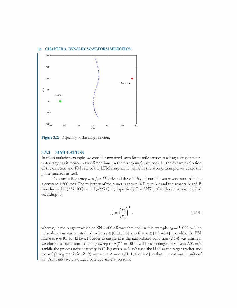
Figure 3.2: Trajectory of the target motion.

3.5.3 SIMULATIONIn this simulation example, we consider two fixed, waveform-agile sensors tracking a single under-water target as it moves in two dimensions. In the first example, we consider the dynamic selectionof the duration and FM rate of the LFM chirp alone, while in the second example, we adapt thephase function as well.

The carrier frequency was fc = 25 kHz and the velocity of sound in water was assumed to bea constant 1,500 m/s. The trajectory of the target is shown in Figure 3.2 and the sensors A and Bwere located at (275, 100) m and (-225,0) m, respectively. The SNR at the ith sensor was modeledaccording to

ηik =(r0

rik

)4

, (3.14)

where r0 is the range at which an SNR of 0 dB was obtained. In this example, r0 = 5, 000 m. Thepulse duration was constrained to be Ts ∈ [0.01, 0.3] s so that λ ∈ [1.3, 40.4] ms, while the FMrate was b ∈ [0, 10] kHz/s. In order to ensure that the narrowband condition (2.14) was satisfied,we chose the maximum frequency sweep as �maxf = 100 Hz. The sampling interval was �Ts = 2s while the process noise intensity in (2.10) was q = 1. We used the UPF as the target tracker andthe weighting matrix in (2.19) was set to � = diag[1, 1, 4 s2, 4 s2] so that the cost was in units ofm2. All results were averaged over 500 simulation runs.

3.5. NARROWBAND ENVIRONMENT 25

Example 1: LFM OnlyWe first test the waveform parameter selection algorithm by choosing λ and b for each sensor whenthe library of waveforms consists of the LFM chirp only. For comparison, we also investigate theperformance of the tracking algorithm when the sensors do not dynamically adapt their transmittedwaveforms.The fixed waveforms in this case correspond to an LFM chirp with the minimum possibleduration λ = 1.3 ms and maximum allowed frequency sweep, and the LFM chirp with the maximumallowed duration λ = 40.4 ms and maximum allowed frequency sweep. Note that the latter config-uration corresponds to the case of the maximum time-bandwidth product, which in conventionalradar and sonar literature, is often considered to be the best choice for tracking applications.

0 10 20 30 40 50 6010

−4

10−3

10−2

10−1

100

101

Time(s)

Ave

rage

d w

eigh

ted

MS

E (

m2 )

λ, b configured

λ = 1.3ms, b = 10 kHz/s

λ = 40.4ms, b = 333 Hz/s

Figure 3.3: Averaged MSE when the sensors dynamically configure LFM chirp waveforms only.

Figure 3.3 shows the averaged MSE obtained when fixed as well as dynamically configuredLFM waveforms are used by the sensors. We observe that the configured waveform offers signif-icantly better performance over the fixed waveform with the maximum time-bandwidth product.The increase in the MSE at k = 15 (30 (s) is due to the fact that, at this time, the target crosses theline joining the sensors. This results in large tracking errors leading to large MSE. The response ofthe algorithm to this situation is seen in Figure 3.4, where the selected pulse length and FM rate areshown for each sensor. We note that the sensors dynamically change the waveform parameters as thetracking progresses. Specifically, at k = 15 (30 s), we observe that both sensors choose b = 0 witha maximum pulse length. This setting changes the LFM chirp into a purely amplitude modulatedsignal which has good Doppler estimation properties. The sensor-target geometry prevents the ac-curate estimation of target range and this configuration permits the tracking algorithm to minimizethe Doppler or velocity errors.


0 5 10 15 20 25 30 35 40 45 500

0.02

0.04

0.06

λA

0 5 10 15 20 25 30 35 40 45 50−5000

0

5000

10000

bA

0 5 10 15 20 25 30 35 40 45 500

0.02

0.04

0.06

λB

0 5 10 15 20 25 30 35 40 45 50−5000

0

5000

10000

Time (s)

b B

Figure 3.4: Typical time-varying selection of waveform parameters (λ, b) by each sensor for the LFMchirp. Sensor A - top two plots, Sensor B - lower two plots.

Example 2: Agile Phase FunctionsIn this example, the two sensors independently choose between the three waveforms in Table 3.1and also dynamically configure their duration and FM rate as in Section 3.5.3. The averaged MSEfor this scenario is shown in Figure 3.5, where we compare the performance of the LFM, EFM, andHFM chirps. We observe that the HFM chirp has the best performance of all the waveforms andis accordingly chosen at each tracking instant. In particular, the performance improvement over theLFM is significant.

3.5.4 DISCUSSIONWhen the waveform is only parameterized by its pulse length, i.e., when the FM rate b = 0, themeasurement noise covariance matrix becomes diagonal. The measurement errors for position in-crease while those for velocity decrease with increasing pulse length. This opposing behavior leadsto a trade-off between the accuracy of range and range-rate estimation. For the GFM waveforms,however, b �= 0 and the estimation errors in range and range-rate become correlated. When themeasurement noise is Gaussian, the conditional variance for range-rate errors given the range maybe shown to be

σ 2r|r = 2c2

4ηf 2c λ

2

for all pulses, and is only dependent on pulse duration. Using the maximum duration would thusresult in the lowest estimation errors for range-rate. The conditional variance on range errors given

3.6. WIDEBAND ENVIRONMENT 27

0 10 20 30 40 50 6010

−4

10−3

10−2

10−1

100

101

Time (s)

Ave

rage

d w

eigh

ted

MS

E (

m2 )

LFM

EFM

HFM

Figure 3.5: Averaged MSE using fixed and configured waveforms and waveform parameters.

the range-rate, however, depends upon g(ξ) in (3.12). It is approximately obtained from N(θk) as

LFM: σ 2r|r = c2

4η�2f

α2

2

EFM: σ 2r|r = c2

4η�2f

exp(λ(α − λ))

(1 + erf(λ))

HFM: σ 2r|r = c2

4η�2f

1

T 2∫∞−∞

1λ√π

exp(− t2

λ2 )1

(T+|t |)2 dt. (3.15)

Intuitively, the configuration algorithm must choose the waveform for which σ 2r|r is the smallest.

From Table 3.1, the FM rate for the HFM pulse is not constrained by the value of λ (and thus Ts) incontrast to the LFM and EFM pulses.Thus, it can always be chosen as the maximum allowed value.For a given �maxf , T can be chosen large and σ 2

r|r in (3.15) is the lowest for the HFM waveform. Itthus provides the best tracking performance as demonstrated in Figure 3.5.

3.6 WIDEBAND ENVIRONMENTIn this section, we consider scenarios where the narrowband condition in (2.14) is not satisfied.Thisimplies that the narrowband model for the received signal developed in Section 2.2.3 is no longerapplicable. We introduce the wideband ambiguity function (WBAF) and develop the CRLB basedon the WBAF.


3.6.1 WIDEBAND SIGNAL MODELWhen the narrowband condition imposed by (2.14) is not satisfied, the received signal model in (2.15)cannot be used since the scaling of the signal envelope is not negligible.This is especially true in sonarapplications where c ≈ 1,500 m/s, and with target velocities in the order of 10 m/s, we must have thetime-bandwidth product TBW 75 to justify the narrowband assumption. As the time-bandwidthproduct of sonar signals is generally much higher than 100, wideband processing is necessary. Insuch situations, the noise-free received signal in (2.13) is given by

sR(t) = √2Re

[√ERs(σ t − τ) exp (j2π(fcσ t))

], (3.16)

where σ = (c − r)/(c + r) > 0 is the Doppler scale and τ = 2r/(c + r) is the delay. Since r c,we have r ≈ cτ/2 and r ≈ c(1 − σ)/2.

The maximum difference in amplitude between s(t (1 − 2r/c)− τ) and its approximations(t − τ) (when the scaling is neglected) occurs when the difference in their arguments is at itsmaximum, which is 2rλ/c, where λ is the signal duration. If�maxf denotes the bandwidth, the signaldoes not change appreciably in an interval less than 1/�maxf . Thus, if the signal satisfies 2rλ/c 1/�maxf , or λ�maxf c/(2r), the error involved in the approximation is small and the scaling maybe neglected. This is the narrowband condition in (2.14). Note, however, that the approximationσ ≈ 1 cannot be made in the phase in (3.16). Accordingly, substituting σ = 1 − (2r/c) in (3.16),and ignoring the scaling, we obtain the narrowband version of the received signal in (2.15). Thus,(2.15) is an approximation of (3.16).

When the environment causes wideband changes in the signal, we must use a processing toolto match it. In this case, the wideband ambiguity function provides a description of the correlationproperties of the signal, and it is given by [48]

WAFs(τ, σ ) = √σ

∫ ∞

−∞s(t)s∗(σ t + τ)dt . (3.17)

As in the narrowband case, the Fisher information matrix is obtained by taking the negative of thesecond derivatives of the WBAF, evaluated at the true target delay and scale [49, 50]. Alternatively,the elements of the Fisher information matrix can be derived directly from the waveform as shownin Appendix B.

3.6.2 WAVEFORM STRUCTUREUpon closer analysis of the results presented in Section 3.5.3, we found that the amplitude envelopeof the waveform plays a significant role in its performance from a tracking perspective. A Gaussianenvelope has often been used in the past [17, 18, 19, 21, 47, 23] due to the flexibility it affordsin computing ambiguity functions and moments of the time and frequency distributions of thesignal. However, the behavior of the phase function in the tails of the Gaussian envelope does notsignificantly affect the waveform’s performance in range and Doppler estimation, since the tailscontain only a small fraction of the signal energy. This can lead to biased conclusions on waveform


performance when different phase functions are considered. In Table 3.1, the LFM and EFM chirpshave larger frequency deviation towards the tails of the envelope while the HFM chirp causes largerfrequency deviations towards the center of the envelope.This explains the superior performance of theHFM chirp in Section 3.5.3. In order to have a fairer comparison between different phase functions,it is necessary to use an amplitude envelope that is uniform. Accordingly, a rectangular envelopewould be most desirable, but the CRLB associated with such waveforms cannot be computed inclosed form since the second moment of its spectrum is not finite [51].

In this and the next chapter, we use a trapezoidal envelope because it avoids the difficultiesassociated with the evaluation of the CRLB for waveforms with a rectangular envelope and yetapproximates it well enough to provide a clearer comparison of phase function performance thanusing a Gaussian envelope. The complex envelope of the signal is defined by (2.12) with

a(t) =

⎧⎪⎨⎪⎩αtf( Ts2 + tf + t), −Ts/2 − tf ≤ t < −Ts/2

α, −Ts/2 ≤ t < Ts/2αtf( Ts2 + tf − t), Ts/2 ≤ t < Ts/2 + tf ,

(3.18)

where α is an amplitude chosen so that s(t) in (2.12) has unit energy.The finite rise/fall time of a(t)is tf Ts/2. Note that the trapezoidal envelope in (3.18) closely approximates a rectangular pulsebut the finite rise/fall time tf permits the evaluation of the CRLB. We define the chirp durationas λ = Ts + 2tf . Note that the frequency sweep �f can be specified by b, λ and ξ(t). In order tocompletely specify a time-frequency signature for the waveform, we must also fix either the initialfrequency f (−λ/2) = f1 or the final frequency f (λ/2) = f2.An additional parameter γ is thereforeintroduced in the phase functions of the considered waveforms which are shown in Table 3.2. Forexample, in the case of the LFM, f (−λ/2) = b/γ = f1 and f (λ/2) = f1 + bλ = f2 can be usedto uniquely determine b and γ once λ, �f and either f1 or f2 are chosen. We fix the larger of f1

and f2 and vary the remaining parameters to obtain various time-frequency characteristics.

Table 3.2: GFM waveforms used in the configuration scenar-ios. The exponent κ defines the time-frequency relationshipof the power-law FM (PFM) chirp waveform.Waveform Phase Function ξ(t) Frequency sweep�f

LFM t/γ + (t + λ/2)2/2 b λ

PFM t/γ + (t + λ/2)κ/κ b λκ−1

HFM ln(t + γ + λ/2) b λγ (γ+λ)

EFM exp(−(t + λ/2)/γ ) b 1γ(exp(− λ

γ)− 1)

3.6.3 SIMULATIONThe simulation study [52] to test the performance of the waveform scheduling algorithm in awideband environment involved two waveform-agile sensors tracking an underwater target moving


in two dimensions,using range and range-rate measurements. In the first example, the library consistsof the HFM chirp only, while in the second example, the selection of the waveform phase functionis also permitted.

The carrier frequency of the transmitted waveform was fc = 25 kHz and the waveformduration ranged within 0.01 s ≤ λ ≤ 0.3 s. The SNR at sensor i at time k was determined accordingto (3.14),where r0 = 500 m was the range at which 0 dB SNR was obtained.We considered a numberof GFM chirps with different time-frequency signatures that are specified by their phase functions,ξ(t/tr ) inTable 3.2 with tr = 1.We define the frequency sweep to be�if = |νi(λi/2)− νi(−λi/2)|,where νi(t) is the instantaneous frequency, and limit it to a maximum of 2 kHz. We fix νi(−λi/2) =fc + 2 kHz (downswept chirps) or νi(λi/2) = fc + 2 kHz (upswept chirps). We then compute bi

and γ i in Table 3.2 for each waveform for any chosen frequency sweep. The sampling interval andthe process noise intensity in (2.10) were�Ts = 2 s and q = 0.01, respectively. The speed of soundin water was taken as c = 1, 500 m/s. The UPF was used as the target tracker and the weightingmatrix in (2.19) was set to � = diag[1, 1, 4 s2, 4 s2] so that the cost was in units of m2. All resultswere averaged over 500 runs. The trajectory of the target is shown in Figure 3.6.

Example 1: HFM OnlyIn the first example, we configured each sensor with the HFM waveform and dynamically selected itsparameters (λ and b) for each sensor so as to minimize the predicted MSE.The actual MSE obtainedin tracking a target, averaged over 500 simulations, is shown in Figure 3.7. For comparison, we alsoshow the MSE that was obtained when the sensor configurations were fixed at the minimum ormaximum durations and the maximum frequency sweep.The improvement in performance in usingdynamic parameter selection is apparent. Figure 3.8 shows the dynamic selection of the frequencysweep that results from the selection of the chirp rate bi by the configuration algorithm. Note thatthe frequency sweep chosen by dynamically selecting the chirp rate is much less than the maximumof 2 kHz. The pulse duration was always selected as the maximum of 0.3 s.

Example 2: Agile Phase FunctionsIn the second simulation example, we permitted the sensors to dynamically select the phase func-tion from among the options in Table 3.2. We allowed the waveform selection to choose betweenhyperbolic, exponential, and power-law FM chirps with κ = 2 and 2.6, in addition to choosing theduration λ and chirp rate b so as to minimize the predicted MSE. Figure 3.9 plots the averaged MSEwhen dynamic parameter selection is used with FM waveforms with different phase functions. Notethat the power-law FM (PFM) chirp with κ = 2 constitutes a linear FM chirp. From Figure 3.9,the PFM chirp with κ = 2.6 performs the best, and we should expect that it will always be chosenas it was indeed observed. The HFM chirp yielded the poorest performance as seen in Figure 3.9.It has been shown that the HFM chirp is optimally Doppler tolerant [35]. This implies that it isminimally Doppler sensitive and should compare poorly with the tracking performance of otherFM waveforms.


−50 0 50 100 150 200 250450

500

550

600

650

700

750

800

x (m)

y (m

)

Sensor A

Sensor B

Figure 3.6: Target trajectory with Sensor A and B located at (-25,500) m and (-25,750) m, respectively.

0 10 20 30 40 50 60

10−2

10−1

100

101

Time (s)

Ave

rage

d M

SE

(m

2 )

λ = 0.01s fixedλ = 0.3 s fixedλ, b configured

Figure 3.7: Averaged MSE when both sensors use HFM chirps.


0 5 10 15 20 25 30 35 40 45 501635

1640

1645

Δ fA (

Hz)

Sensor A

0 5 10 15 20 25 30 35 40 45 501580

1600

1620

1640

1660

Δ fB (

Hz)

Time (s)

Sensor B

Figure 3.8: Dynamic selection of the frequency sweep �if , when both sensors i = A, B use HFMwaveforms [52].

0 5 10 15 20 25 30 35 40 45 50

10−2

10−1

100

101

Time (s)

Ave

rage

d M

SE

(m

2 )

PFM, κ = 2PFM, κ = 2.6EFMHFMPFM, κ = 2PFM, κ = 2.6EFMHFM

Figure 3.9: Comparison of averaged MSE using various waveforms when the allowed frequency sweepis 1 kHz (dotted) and 2 kHz (solid) [52].


3.6.4 DISCUSSIONAs the variance of the range-rate estimation errors depends inversely on the pulse duration, thealgorithm attempts to minimize these errors when the maximum allowed pulse length is used. Onthe other hand, range estimation errors can be minimized by using the maximum time-bandwidthproduct. However, the correlation between the errors increases with increasing frequency sweep,thereby reducing the ability of the waveform to estimate range and range-rate simultaneously. Thus,there is a trade-off in the choice of frequency sweep and this is reflected in the selections made bythe configuration algorithm.

35

C H A P T E R 4

Dynamic Waveform Selectionfor Tracking in Clutter

The tracking of a target with observations that do not guarantee perfect detection in an environmentthat includes clutter is significantly complicated by the uncertainty in the origin of the measurements.This introduces new trade-offs in the waveform selection process [53]. In this chapter, we examinethe problem of selecting and configuring waveforms for tracking targets in clutter with imperfectdetections. We present a methodology to predict the mean square error (MSE) in this scenario.Using the probabilistic data association filter, the algorithm is first applied to the tracking of a singletarget and then extended to multiple targets.

4.1 SINGLE TARGET

In this section, we present the application of the waveform-agile tracking algorithm in an environ-ment that includes a single target that is observed in the presence of clutter with nonunity probabilityof detection. We begin by augmenting the observation model described in Section 2.2.3 to reflectthe fact that at each sampling instant, each sensor obtains more than one measurement. We alsointroduce a model for false alarms due to clutter.

4.1.1 OBSERVATIONS MODELWhen clutter is present in the observation space, there are likely to be false alarms due to clutter.Since we also assume imperfect detection, sensor i will obtain mik ≥ 0 measurements at time k. Wedefine the measurement vector for sensor i at time k as

Zik = [z1

k,i , z2k,i , . . . , z

mikk,i ] , (4.1)

where zmk,i = [ri,mk ri,mk ]T ,m = 1, . . . , mik . We also define Zk = [ZA

k ZBk ] as the full measurement

at time k. The probability that the target is detected (i.e., that Zik includes a target-originated

measurement) is given byP idk .The target-originated measurements at each sensor are given by (2.16).

4.1.2 CLUTTER MODELWe assume that the number of false alarms follows a Poisson distribution with average ρV ik , whereρ is the density of the clutter and V ik is the validation gate volume. The validation gate is a regionin the observation space centered on the next predicted observation [3]. Only observations that fall

36 CHAPTER 4. DYNAMIC WAVEFORM SELECTION FOR TRACKING IN CLUTTER

within this region are validated as having been potentially originated by the target. The probabilitythat m false alarms are obtained is

μ(m) = exp(−ρV ik )(ρV ik )mm! . (4.2)

We also assume that the clutter is uniformly distributed in the volume V ik . The probability ofdetection at time k is modeled according to the relation

P idk = P

11+ηi

k

f ,

where Pf is the desired probability of false alarm and ηik is the SNR at sensor i.

4.1.3 TARGET TRACKING WITH PROBABILISTIC DATA ASSOCIATIONAs described in Section 2.1.1, we use a particle filter as the tracker. As is often the case, we use thekinematic prior, p(Xj

k |Xj

k−1), as the importance density. From (2.5), the weights are then propor-

tional to the likelihood function p(Zk|Xjk , θk) as in (2.7). Next, we present the likelihood function

for this scenario.Since there is uncertainty in the origin of the measurements, the target tracker must also

estimate the measurement-to-target association. One method of filtering in this scenario is to treateach individual measurement, in turn, as target-originated, and all the other measurements as beingdue to clutter. This gives rise tomik associations, each of which is weighted with its probability giventhe measurements, and incorporated in the filter update. This approach is known as probabilisticdata association [3] and computes the likelihood as an average over all possible data associations.The measurements obtained at each sensor are assumed to be independent.Therefore, the likelihoodfunction is the product of the likelihood functions for each sensor and is given by

p(Zk|Xk, θk) =∏i=A,B

p(Zik|Xk, θ ik) . (4.3)

To derive p(Zik|Xk, θ ik), we assume that the target generates at most one measurement which is

detected with probabilityP idk ,while the remaining measurements consist of false alarms due to clutter.The measurement Zi

k must therefore be comprised of either one target-originated measurementtogether with mik − 1 false alarms, or mik false alarms. In the former case, the probability that anyone of themik measurements was generated by the target is equal, and as a result, all measurement-to-target associations are equiprobable. The probability of obtaining the total measurement Zi

k , giventhat the target was detected, will therefore include the probability that each individual measurementzmk,i, m = 1, . . . , mik in (4.1) was generated by the target, weighted by the measurement’s association

4.1. SINGLE TARGET 37

probability. Thus, we can directly write the likelihood function for sensor i in (4.3) as [54]

p(Zik|Xk, θ ik) = (1 − P idk )μ(m

ik)(V

ik )

−mik

+ P idk (Vik )

−(mik−1)μ(mik − 1) · 1

mik

mik∑m=1

p(zmk,i |Xk, θ ik) . (4.4)

4.1.4 WAVEFORM SELECTION IN THE PRESENCE OF CLUTTERThe algorithm for waveform selection presented in Chapter 3 assumes that there is only one mea-surement and that it is target-originated. While the algorithm structure remains the same whenclutter and imperfect detection are considered, the computation of the predicted cost must reflectthe uncertainty in the origin of the measurements. Next, we describe the method used to approximatethe predicted cost using the unscented transform.

We assume that the sigma points X n corresponding to a distribution with mean Xk|k−1 andcovariance Pk|k−1 have been computed according to (3.7). As before, we wish to approximate thecovariance Pk|k(θk) that would be obtained if a waveform characterized by its parameter vector θk isused to obtain a measurement at time k.For sensor i, a transformed set of sigma points Z i

n = hi(X n)

is computed. Then, as in (3.8) and (3.9), we calculate the covariances

P izz =2N+1∑n=0

Wn

(Z in − Z

) (Z in − Z

)T, (4.5)

P ixz =2N+1∑n=0

Wn

(X n − X

) (Z in − Z

)T, (4.6)

where

Z =2N+1∑n=0

WnZ in and X =

2N+1∑n=0

WnX n .

Note that the expectation in (2.19) is also over all realizations of the clutter and thus over allpossible measurement-to-target associations.The calculation of Pk|k(θk) should reflect this fact. In-tuitively, if there was no uncertainty in the origin of the measurements, all the information containedin the target-originated measurement could be unambiguously used to reduce the covariance of thestate estimate as in (3.10). As is evident from (4.4), each measurement, whether target-generatedor not, contributes to the update. The measurements that are not target-generated thus limit thereduction in the covariance during the update step. When probabilistic data association is used, ithas been shown that the expected covariance of the state after an update with the measurement atsensor i is given by [55]

P ik|k(θik) = Pk|k−1 − qi2kP

ck|k , (4.7)


where P ck|k is the update due to the true measurement. Using the unscented transform, this updateis given by

P ck|k = P ixz(Pizz + (N(θ ik))

−1P ixzT. (4.8)

The scalar qi2k in (4.7) lies between 0 and 1 and is called the information reduction factor.From (3.10),(4.7), and (4.8), we see that it serves to lower the reduction in the covariance that would have beenobtained if there was no uncertainty in the origin of the measurements due to clutter. The infor-mation reduction factor depends upon P idk , ρ and V ik , and its computation involves a complicatedintegral which has to be evaluated by Monte Carlo methods. However, in this work, we use someapproximations that are available in the literature [56].

Note that the information reduction factor is different for each sensor. This requires that theupdate in (4.7) be performed sequentially for each sensor. Accordingly, we first use the measurementof Sensor A to obtain PAk|k(θ

Ak ) using (4.7) and (4.8). A second update, using the measurements of

Sensor B, is then carried out with Pk|k−1 = PAk|k(θAk ) in (4.7) to yield PBk|k(θ

Bk ). The second update

requires another computation of all the covariance matrices in (4.8) using the unscented transformwith i = B. Note that PBk|k(θ

Bk ) is the final predicted covariance Pk|k(θk) as it includes information

from both sensors A and B. The approximate cost J (θk) in (2.19) is then computed as the traceof �Pk|k(θk).

4.1.5 SIMULATIONThe waveform library used in this simulation is the same as that used in Section 3.6.3, and thephase functions and the bandwidth are shown in Table 3.2. In this example, however, we use radarsensors and assume that the received signal satisfies the narrowband assumption. Figure 4.1 showsthe instantaneous frequencies of these waveforms for a duration of λ = Ts + 2tf = 100 μs and afrequency sweep of �f = 14 MHz.

Our simulations consist of two radar sensors tracking a target that moves in two dimensions.The signal duration was restricted to the range 10 μs ≤ λik ≤ 100 μs while the carrier frequency wasfc = 10.4 GHz. For each waveform considered, the frequency sweep was determined by selecting thestart and end points of the desired time-frequency signature as in Figure 4.1, with the restriction thatthe maximum frequency sweep was 15 MHz.The FM rate bik and the parameter γ i in Table 3.2 werethen computed from the frequency sweep and the duration of the waveform. The sampling intervalin (2.10) was �Ts = 250 ms. The SNR was computed according to (3.14) where r0 = 50 km wasthe range at which a 0 dB SNR was obtained and the probability of false alarm was Pf = 0.01. Thevalidation gate was taken to be the 5-sigma region around the predicted observation [3]. The targettrajectory was generated with the initial state X0 = [0 0 100 800]T. The process noise intensityin (2.10) was q = 0.1, while the covariance of the initial estimate provided to the tracker wasP0 = diag[1, 000 1, 000 50 50]. Sensor A was located at (0, -15,000) m and Sensor B at (15,6314,995) m.The standard particle filter was used as the tracker, and the weighting matrix in (2.19) wasset to � = diag[1 1 1 s2 1 s2] so that the cost function in (2.19) had units of m2. All results were


0 0.1 0.2 0.3 0.4 0.5 0.6 0.7 0.8 0.9 1

x 10−4

2

4

6

8

10

12

14

x 106

Time (s)

Fre

quen

cy (

Hz)

PFM κ = 2.8

LFM

EFM

HFM

Figure 4.1: Time-frequency plots of generalized FM chirp waveforms (downsweep - solid lines, upsweep- dotted lines) with duration 100 μs and frequency sweep 14 MHz.

averaged over 500 Monte Carlo simulations. When more than four continuous measurements felloutside the validation gate for either sensor, the track was categorized as lost.

Example 1: Linear Frequency Modulated (LFM) Chirp OnlyIn the first example, we consider the performance of the dynamic parameter configuration algorithmwhen only the LFM chirp is transmitted by the sensors. Specifically, we compare the performanceof configuring the duration and FM rate (or equivalently frequency sweep) of the transmitted LFMchirp to that obtained when an LFM chirp is used with fixed parameters. For the fixed LFM chirps,we consider the shortest and longest allowable durations and the maximum allowed frequency sweep.The averaged MSE, computed from the actual error in the estimate and conditioned on convergencedue to possible lost tracks, is shown in Figure 4.2 for two clutter densities,ρ = 0.0001 and ρ = 0.001false alarms per unit validation gate volume. It is apparent that the configuration algorithm providesimproved performance. lost by the tracker. Specifically, when the fixed waveforms were used, anaverage of 25% and 38% of tracks were lost by the 10 μs and 100 μs pulse, respectively. Thedynamically configured waveform, however, lost only 0.7% of the tracks. This can be attributed to


0 1 2 3 4 5 610

1

102

103

104

Time (s)

Ave

rage

d M

SE

(m

2 )

λ min

λ max

Configured

Figure 4.2: Comparison of averaged MSE using fixed and configured LFM chirps only. Clutter densityρ = 0.0001 (solid lines) and ρ = 0.001 (dotted lines) [22].

the number of false alarms that appear in the measurements at each sensor, which in turn is directlyproportional to the validation gate volume. In Figure 4.3 we compare the volume for the three LFMwaveforms for ρ = 0.0001, and find that the configured waveform results in a much lower volumefor both sensors. The validation gate volume for sensor i is proportional to the determinant of thematrix (P izz +N(θ ik)) in (4.8). As the search over the space of waveforms proceeds, it is apparentthat this determinant will be minimized. In addition, the information reduction factor qi2 in (4.7)increases as the validation gate volume decreases [55]. Thus, a waveform that results in a smallervalidation gate also contributes more towards reducing the covariance of the state estimate.

Example 2: Agile Phase FunctionIn this simulation, in addition to dynamically configuring the duration and FM rate, we also selectthe phase function ξ(t/tr ) in (2.12) of the generalized chirp waveforms. The set of waveformsavailable to the sensors includes the power-law FM (PFM) chirp with varying κ , the hyperbolicFM (HFM) and exponential FM (EFM) chirps as described in Table 3.2. For the simulations,we chose κ = 2, 2.8, 3. Recall that κ = 2 yields an LFM waveform. For this example the clutterdensity was ρ = 0.0001 false alarms per unit validation gate volume. Figure 4.4 shows the averagedMSE, conditioned on convergence, that is obtained when the phase function is dynamically selected,in addition to the waveform duration and FM rate. For comparison, the averaged MSE for each


0 1 2 3 4 5 610

3

104

105

106

VA k

Sensor A

0 1 2 3 4 5 610

3

104

105

106

107

Time (s)

VB k

Sensor B

λ min

λ max

Configured

Figure 4.3: Comparison of averaged validation gate volume using fixed and configured LFM chirps onlywith clutter density ρ = 0.0001 [22].

generalized chirp is also shown; this is obtained when the generalized FM chirp has its duration andFM rate configured as in Example 1 for the LFM.

We find that there is some improvement in the tracking performance when the phase functionis dynamically selected. A typical waveform selection for one simulation run is shown in Figure 4.5.We note that the HFM and the EFM chirps are chosen at the first few instants while the PFMchirp with κ = 3, and hence parabolic instantaneous frequency, is used later. The LFM chirp andthe PFM chirp with κ = 2.8 are not selected at all.

4.1.6 DISCUSSIONIn order to understand the waveform selection behavior, note that when the tracking starts, the rangeand range-rate of the target are poorly known and must be simultaneously estimated. Waveformsthat offer little correlation between the estimation errors should accordingly be selected. Figure 4.6shows the correlation coefficient for the waveforms available to the tracker for a duration of 100μs and a frequency sweep of 15 MHz. Note that the HFM and EFM chirps have smaller corre-lation coefficients than the PFM chirps. When the range and range-rate estimates of the targets


0 1 2 3 4 5 6

101

102

103

Time (ms)

Ave

rage

d M

SE

(m

2 )

LFMPFM κ = 2.8PFM κ = 3.0EFMHFMConfigured

Figure 4.4: Comparison of averaged MSE,conditioned on convergence,with and without phase functionagility [22].

improve, it is possible to utilize the correlation between the estimation errors to improve the trackingperformance. At this stage, waveforms that provide considerable correlation become more suitable.Thus, the conditional variance of the range given the range-rate becomes an important feature. Asseen in Figure 4.6, the PFM chirps offer lower values than the EFM and HFM chirps. However,minimization of the validation gate volume also occurs during the dynamic selection procedure.Thevolume for Pzz = diag[5, −50, −50, 1, 000] and an SNR of 20 dB is also shown in Figure 4.6.Note that the PFM chirp with κ = 3 offers a lower volume than the LFM chirp and is thereforealways selected during the later stages of the tracking sequence.

4.1.7 PERFORMANCE UNDER DIFFERENT CHOICES OF THEWEIGHTING MATRIX

The choice of the weighting matrix � in (2.19) can have significant impact on the performanceof the algorithm. In order to investigate this dependence, we conducted simulations in which the


0 1 2 3 4 5 6LFM

PFM (2.8)

PFM (3.0)

EFM

HFMSensor A

0 1 2 3 4 5 6LFM

PFM (2.8)

PFM (3.0)

EFM

HFM

Time (s)

Sensor B

Figure 4.5: Typical waveform selection when the phase function is configured together with the durationand FM rate of the waveform [22].

cost function depended only on position variance (� = diag[1, 1, 0, 0]), and only on velocityvariance (� = diag[0, 0, 1, 1]).

Figure 4.7 compares the position MSE achieved by the phase-function-agile waveformunder different choices of � in (2.19). In Figure 4.7, note that the performance is best when� = diag[1, 1, 1 s2, 1 s2], i.e., when both position and velocity variances contribute to the costfunction. This is due to the fact that the target tracker uses both velocity and position estimates attime k − 1 to estimate the position at time k. A poor estimate of velocity thus also contributes toposition errors.The performance in velocity estimation in various cases is shown in Figure 4.8. It canbe noted from Figure 4.7 that the difference in performance is the greatest between approximately1.75 s and 4.75 s during the tracking sequence. This is due to the fact that during this period, thetarget is furthest from both sensors leading to poor SNR. Thus, the estimation errors in range andrange-rate are high. Accordingly, the tracker places a greater dependence on the kinematics model,which, as stated earlier, can only provide accurate information if both position and velocity are wellestimated. A typical waveform selection sequence when the cost function depends on position vari-ance only and velocity variance only is shown in Figures 4.9 and 4.10, respectively. It is interesting


LFM PFM(2.8) PFM(3.0) EFM HFM0

0.5

1

Cor

rela

tion

coef

ficie

nt


2

4x 10

8

Val

idat

ion

gate

volu

me


20

40

Con

ditio

nal

varia

nce

(dB

)

Waveform type

Figure 4.6: Correlation coefficient (top), validation gate volume (middle), and conditional variance ofrange given range-rate (bottom) for the waveforms used in Section 4.1.5. The correlation coefficient forthe HFM chirp is negligibly small [22].

0 1 2 3 4 5 6 710

−1

100

101

102

103

104

Time(s)

Ave

rage

d P

ositi

on M

SE

Λ = diag[1 1 0 0]Λ = diag[0 0 1 1]

Λ = diag[1 1 1s2 1s2]

Figure 4.7: Comparison of averaged position MSE, conditioned on convergence, under different choicesof the weighting matrix � in (2.19).


0 1 2 3 4 5 6

101

102

Time(s)

Ave

rage

d ve

loci

ty M

SE

Λ = diag[1 1 0 0]Λ = diag[0 0 1 1]

Λ = diag[1 1 1s2 1s2]

Figure 4.8: Comparison of averaged velocity MSE, conditioned on convergence, under different choicesof the weighting matrix � in (2.19).

0 1 2 3 4 5 6LFM

PFM (2.8)

PFM (3.0)

EFM

HFMSensor A

0 1 2 3 4 5 6LFM

PFM (2.8)

PFM (3.0)

EFM

HFM

Time (s)

Sensor B

Figure 4.9: Typical waveform selection when the cost function depends on position variance alone.


0 1 2 3 4 5 6LFM

PFM (2.8)

PFM (3.0)

EFM

HFMSensor A

0 1 2 3 4 5 6LFM

PFM (2.8)

PFM (3.0)

EFM

HFM

Time (s)

Sensor B

Figure 4.10: Typical waveform selection when the cost function depends on velocity variance alone.

to note that the behavior is similar to that observed in Figure 4.5 for the case where both variancescontribute to the cost function.

4.2 MULTIPLE TARGETS

In this section, we extend the waveform selection algorithm developed in Section 4.1 to a scenariothat includes multiple targets, clutter and missed detections [57]. Specifically, assuming that thenumber of targets is known, we show how waveform selection can be used to minimize the totalMSE of tracking multiple targets and present a simulation study of its application to the tracking oftwo targets. We begin by extending the target dynamics and observations models of Sections 2.2.1and 4.1.1, respectively, to multiple targets.

4.2.1 TARGET DYNAMICSLet

Xk = [x1k

T, . . . , xSk

T ]T (4.9)

represent the state of S targets that move in a two-dimensional space. The state of target s, s =1, . . . , S is xsk = [xsk ysk xsk ysk]T , where xsk and ysk correspond to the position, and xsk and ysk to thevelocity at time k in Cartesian coordinates. The dynamics of each target are modeled by a linear,

4.2. MULTIPLE TARGETS 47

constant velocity model given byxsk = F xsk−1 + ws

k , (4.10)

where wsk is a white Gaussian noise sequence that models the process noise. The constant matrix F

and the process noise covariance matrix Q are as given by (2.10).

4.2.2 MEASUREMENT MODELAt each sampling epoch, both sensors, Sensor A and Sensor B, obtain range (r) and range-rate (r)measurements of each target. At time k, the measurement corresponding to target s obtained atsensor i, is given by

zs,ik = hi(xsk)+ vs,ik , (4.11)

where vs,ik is a white Gaussian noise sequence that models the measurement error. We assume thatvs,ik in (4.11) is independent between all targets and sensors, and that vs,ik and ws

k in (4.10) areuncorrelated for all targets. The nonlinear function hi(xsk) = [rs,ik r

s,ik ]T , where

rs,ik =

√(xsk − xi)2 + (ysk − yi)2

rs,ik = (xsk(x

sk − xi)+ ysk(y

sk − yi))/r

s,ik ,

and sensor i is located at (xi, yi).

4.2.3 CLUTTER MODELAs in Section 4.1.2, we assume that the number of false alarms at sensor i follows a Poisson distribu-tion with average ρV ik , where ρ is the density of the clutter, and V ik is the validation gate volume [3].The validation gate volume for target s at sensor i is V s,ik , and V ik is the union of the volume for eachof the S targets at sensor i. The probability that m false alarms are obtained is given by (4.2). Wealso assume that the clutter is uniformly distributed in the volume V ik . The probability of detectionat time k is modeled according to the relation

Ps,idk

= P

1

1+ηs,ik

f , (4.12)

where Pf is the desired false alarm probability and ηs,ik is the SNR at sensor i corresponding totarget s.

4.2.4 MULTIPLE TARGET TRACKING WITH JOINT PROBABILISTIC DATAASSOCIATION

We use a particle filter tracker to recursively estimate the probability distribution p(Xk|Z1:k, θ1:k)of the target state, given the sequence of observations Z1:k and waveform vectors θ1:k up to timek. Each particle consists of a concatenation of the states of each individual target and is thus a


4S × 1 vector. When multiple targets are to be tracked in the presence of clutter, the measurement-to-target association must also be estimated. Using arguments similar to Section 4.1.3 for a singletarget in clutter, we present the likelihood function for the case of two targets in clutter. Withthe kinematic prior used as the sampling density as in (2.6), the weights are proportional to thelikelihood function. Since the measurement noise at each sensor is assumed to be independent, thetotal likelihood function is given by (4.3), and we need only derive p(Zi

k|Xk, θ ik), the likelihoodfunction for sensor i.

When the targets are well separated in the observation space, the likelihood function factorizesinto S components, one for each target, so that

p(Zik|Xk, θ ik) =

S∏s=1

p(Zs,ik |xsk, θ ik) , (4.13)

where Zs,ik ⊂ Zi

k is a set consisting of the observations in the validation gate of target s. Such ascenario corresponds to the case where the validation gates for each of the targets do not intersect.In this situation, the joint tracking of the targets reduces to tracking each target independently [58].Assuming that each target produces at most one measurement, the likelihood functions in (4.13)are as in (4.4)

p(Zs,ik |xsk, θ ik) = (1 − P

s,ik )μ(ns)(V

s,ik )

−ns

+ Ps,ik (V

s,ik )

−(ns−1) · μ(ns − 1)1

ns

ns∑m=1

ps,im ,

where ns is the number of observations in the validation gate for target s and ps,im = p(zs,ik,m|xsk, θ ik)is the probability that the mth measurement in Zs,i

k (or equivalently, the validation gate region fortarget s) was originated from target s.

When the targets are not well separated, their validation gates may overlap, as shown inFigure 4.11 for S = 2 targets. Here, n1 and n2 are the number of measurements that are validatedexclusively for Target 1 and Target 2, respectively, while n3 is the number of measurements validatedfor both targets. In this case, the factorization in (4.13) does not hold, and the tracker must estimatethe states of each target jointly. We then have

p(Zik|Xk, θ ik) =

R∑r=1

p(Zik|�r,Xk, θ ik)p(�r) ,


rang

e−ra

te

Target 1Target 2

Validation gates

range

n1

n2

n3

mi

k= n1 + n2 + n3

Figure 4.11: Overlapping validation gates in observation space for two targets.

where �r is the measurement-to-target association [3]. By exhaustively enumerating all possibleassociations when both targets, either target, or no targets are detected, it can be shown that

p(Zik|Xk, θ ik) ∝ (1 − P

1,idk)(1 − P

2,idk)

+ mikρ−1P

1,ik (1 − P

2,ik )

n1 + n3

n1+n3∑m=1

p1,im

+ mikρ−1P

2,ik (1 − P

1,ik )

n2 + n3

n2+n3∑m=1

p2,im

+ mik(mik − 1)ρ−2P

1,ik P

2,ik

n1n2 + n2n3 + n1n3

n1+n3∑l=1

n2+n3∑m=1

p1,il p

2,im . (4.14)

Note that each target produces at most one measurement and the last summation in (4.14) mustexclude all combinations that violate this fact. Although this was only shown for S = 2 targets, itcan be extended to an arbitrary number of targets as in [3].

4.2.5 DYNAMIC WAVEFORM SELECTION AND CONFIGURATIONThe waveform selection algorithm seeks the waveform for each sensor that minimizes the sum ofthe predicted MSE for all targets at the next time step. The cost function to be minimized is still


defined as in (2.19) but with the target state defined as in (4.9).The rectangular grid search algorithmof Chapter 3 is again used; however, the algorithm for approximating the predicted MSE consistsof an extension to multiple targets of the algorithm presented in Section 4.1.4. This method ofapproximating the predicted cost is presented next.

Let Pk−1|k−1 represent the covariance of the state estimate at time k − 1. We first obtain thepredicted covariance at time k using the target dynamics model in (4.10) as

Pk|k−1 = FPk−1|k−1FT +Q .

In order to obtain Pk|k(θk), the estimate of the updated covariance that would result if a waveformparameterized by θk was used at time k, we update each of the 4 × 4 block matrices P sk|k−1, alongthe diagonal of Pk−1|k−1, sequentially for each sensor.

Sigma points X sn are first computed from the probability density function whose mean and

covariance are given by the predicted position of target s and P sk|k−1, respectively, [29], as in (3.7).

The sigma points are transformed to yield Zs,in = hi(X s

n). The covariance matrix P s,izz of Zs,in ,

and the cross-covariance P s,ixz between X sn and Zs,i

n are computed analogously to (4.5) and (4.6),respectively. The updated covariance is computed as

Ps,ik|k(θ

ik) = P sk|k−1 − q

s,i2kP ck|k (4.15)

P ck|k = P s,ixz (Ps,izz + (Ns(θ ik))

−1P s,ixzT

(4.16)

where qs,i2kis an information reduction factor [55].The updates in (4.15) and (4.16) are performed for

Sensor A to yield P s,Ak|k (θAk ). The update for Sensor B follows the same procedure but with P sk|k−1

in (4.15) replaced by P s,Ak|k (θAk ) to yield P sk|k(θk) = P

s,Bk|k (θ

Bk ). Note that the covariance matrices

in (4.16) must be re-evaluated for the second update. Once each of the P sk|k(θk) has been evaluated,we form Pk|k(θk) = diag[P 1

k|k(θk), . . . , PSk|k(θk)] and obtain J (θk) ≈ trace(�Pk|k(θk)).

4.2.6 SIMULATIONIn this simulation study, Sensor A and Sensor B were located at (3,000, -16,000) m and(3,000, 20,400) m, respectively, and tracked two targets as they moved in a two-dimensionalspace. The target trajectories were constructed with x1

0 = [2, 000 − 1, 000 −100 800]T and x20 =

[1, 000 −1, 000 100 800]T . In (2.10), q = 1 and the sampling interval was�Ts = 0.25 s.The clut-ter density was ρ = 0.0001 false alarms per unit validation gate volume while the probability of falsealarm was Pf = 0.01. The SNR was modeled as (4.12) with r0 = 50 km. We used the standardparticle filter as the target tracker, and the weighting matrix in (2.19) was the 8 × 8 identity matrixwith appropriate units so that the MSE had units of m2. Initially only Target 1 was present in theobservation space and Target 2 was assumed to be detected at k = 8. Each target was tracked for 25time steps (a total of 6.25 s). The initial position given to the tracker for target s was drawn from anormal distribution with mean xs0 and variance P0 = diag[4,000, 4,000 100, 100]. All results were


averaged over 500 Monte Carlo runs, conditioned on convergence of the tracker. We defined conver-gence to imply that the target-originated measurements for each target fell outside their validationgates at either sensor no more than five times during the entire tracking sequence.

Figure 4.12 shows the averaged MSE obtained using the waveform selection and configurationalgorithm.The abrupt increase in the MSE at k = 8 (1.75 (s) is due to the fact that the second targetappears at this instant. Similarly, the drop in MSE at k = 26 (6.25 (s) is due to the fact that thefirst target disappears at this time. For comparison, we also show the averaged MSE obtained whenthe waveform duration and FM rate may be configured dynamically but the phase function is fixed.We observe that, with phase function agility, the tracking performance improves. In particular, theperformance is significantly better than that achieved by the LFM chirp, which is a common choicein radar applications. A typical waveform selection during the tracking sequence is presented inFigure 4.13. Note that the waveforms selected include only the HFM and the PFM chirp withκ = 3, which corresponds to a parabolic instantaneous frequency. Interestingly, the LFM chirp isnever selected and the selection behavior is similar to that in Figure 4.5.

0 1 2 3 4 5 6 7 8

103

104

Time (s)

Ave

rage

d M

SE

(m

2 )

LFMPFM κ = 2.8PFM κ = 3EFMHFMConfigured

Figure 4.12: Averaged MSE using waveforms with fixed and agile phase functions.


1 2 3 4 5 6 7 8LFM

PFM(2.8)

PFM(3.0)

EFM

HFMSensor A

1 2 3 4 5 6 7 8LFM

PFM(2.8)

PFM(3.0)

EFM

HFM

Time (s)

Sensor B

Figure 4.13: Typical waveform selection during the tracking sequence.

4.2.7 DISCUSSIONThe behavior of the waveform selection algorithm as demonstrated in Figure 4.13, is due to the factthat, at the start of the tracking, the uncertainty in position and velocity are both large and the rangeand range-rate have to be estimated independently; thus waveforms with minimal range-Dopplercoupling should be expected to be chosen. It has been demonstrated in Section 4.1.6, that the HFMchirp has this feature. When the uncertainty in the target state estimate is reduced, it is possible toobtain a reduction in estimation errors by exploiting the range-Doppler coupling. The power chirpwith κ = 3 has been shown to provide a lower variance on range errors conditioned on range-ratethan the other chirps while still minimizing the validation gate volume. Therefore, the algorithmselects this waveform during the later stages of the tracking sequence. Note that this behavior isrepeated when the second target appears at time k = 8. At this time, the uncertainty in the stateestimate again increases and the algorithm chooses the HFM chirp to independently estimate therange and range-rate of the second target.

53

C H A P T E R 5

ConclusionsRecent advances in electromagnetics, processing, and radio frequency analog devices afford a newflexibility in waveform design and application. This technology is now being used in the researchand development of sensors that can dynamically change the transmit or receive waveform in orderto extract information that can contribute optimally to the overall sensing objective. Thus, a newparadigm of waveform-agile sensor processing has been exposed, which promises significant im-provements in active sensor system performance by dynamic adaptation to the environment, target,or information to be extracted.

In this work, we presented new algorithms for waveform-agile sensing for target tracking. Weconsidered various scenarios of this application, depending on the level of clutter embedded withthe target. Specifically, we considered tracking in narrowband and wideband environments with noclutter, as well as with clutter, both for single and multiple targets.

Specifically, we considered the selection and configuration of waveforms for waveform-agilesensors so as to minimize a tracking error. In contrast with past research on this problem, weconsidered a nonlinear observations model to track a target moving in two dimensions as well as theuse of waveforms with nonlinear time-frequency signatures. Our method of computing the predictedmean square error (MSE) is based on the unscented transform and the Cramér-Rao lower bound(CRLB) on the measurement error. To track a single target in clutter, we used a particle filter withprobabilistic data association, while joint probabilistic data association was used in the tracking ofmultiple targets. The particle filter provides robustness with respect to observation nonlinearitiesand sensor positioning. The waveform selection algorithm was applied to several different scenariosincluding narrowband and wideband environments, clutter and imperfect detection, and single aswell as multiple targets. For each case, we presented simulation studies to demonstrate that thealgorithm provides approximately 10 dB reduction in MSE as compared to a nonadaptive system.

5.1 SUMMARY OF FINDINGS

A summary of the major conclusions we derived from our work is given below.

• Waveforms that maximize the time-bandwidth product do not necessarily provide the besttracking performance.The idea of using waveforms with the largest allowable duration and the maximum possiblebandwidth is well established in radar. This configuration minimizes the conditional varianceof range given range-rate estimates. However, such waveforms necessarily correlate the rangeand range-rate estimation errors and are not suitable when both these parameters have tobe independently estimated. As we described in Chapter 4, when the tracking of a target

54 CHAPTER 5. CONCLUSIONS

commences, neither parameter is known with adequate accuracy to achieve variance reductionby conditioning. Thus, waveforms that result in correlated errors in range and range-ratemeasurements are not appropriate. It is interesting to note that bats, which use sonar to locateand capture their prey, do not necessarily use waveforms that maximize the waveform time-bandwidth product.They vary the transmitted waveforms through various phases of the search,approach, and capture of their prey [59, 60]. That our algorithm behaves similarly to nature,provides in our opinion, a support of its validity.

• Nonlinear frequency modulated (FM) waveforms offer significant advantages over thelinear FM waveform.The linear FM chirp has enjoyed widespread popularity in radar and sonar whereas nonlinearFM chirps have been relatively less used [32]. However, we have shown in Section 4.1.6 thatthe hyperbolic, exponential, and power-law FM chirp, with parabolic instantaneous frequency,provide better tracking performance than the linear FM chirp, especially when they are usedin a dynamic, adaptive manner. Once again, the correspondence with nature is remarkable.Dolphins and bats are known to use nonlinear FM chirps and exploit their properties, such asDoppler tolerance [35, 59].

• Dynamic waveform adaptation can reduce tracking error.It has been recently shown [21] that for an LFM chirp waveform, the maximum informationabout the target state can be obtained by a waveform with a frequency sweep rate that iseither the maximum or the minimum possible, given a set of constraints on the waveformsuch as average power, duration, and frequency sweep rates.This result was derived for a linearobservations model and an information theoretic criterion. When the performance metric isthe tracking MSE and when nonlinear observations models are used, we have demonstratedimproved performance by dynamically selecting both the waveform duration and the frequencysweep rates of GFM chirps.

• Dynamic waveform adaptation is more effective in the presence of clutter than in clutter-free environments.When clutter is present in the observation space, there is uncertainty in the origin of themeasurements. Accordingly, a validation gate must be set up and only those measurementsthat fall within the gate are considered as potentially target-originated. If clutter is assumed tobe uniformly distributed, the number of false alarms is directly proportional to the validationgate volume. Since a large number of false alarms negatively impacts tracking performance,the control of the validation gate volume becomes important. The validation gate volumedepends upon the choice of waveform as was shown in Section 4.1.6, and this provides anadded dimension in which waveform adaptation can be exploited when used in the presenceof clutter.

55

A P P E N D I X A

CRLB evaluation for GaussianEnvelope GFM Chirp from the

ambiguity functionIn this appendix, we derive the elements of the Fisher information matrix corresponding to GFMchirps (2.12) with a Gaussian envelope. The elements are obtained by computing the Hessian of thenarrowband ambiguity function and evaluating it at the origin of the delay-Doppler plane.

As in (3.11), define the complex envelope as

s(t) =(

1

πλ2

) 14

exp

(− t2

2λ2

)exp (j2πbξ(t)), (A.1)

where λ parameterizes the duration of the Gaussian envelope, b is the frequency modulation (FM)rate, and ξ(t) is a real valued, differentiable phase function. The narrowband ambiguity function isgiven by (2.18) and is repeated below for convenience:

AFs(τ, ν) =∫ ∞

−∞s(t + τ

2

)s∗(t − τ

2

)exp(−j2πνt)dt. (A.2)

Substituting (A.1) in (A.2)

AFs(τ, ν) =∫ ∞

−∞1

λ√π

exp{−(1/λ2)

(t2 + τ 2/4

)}exp {j2πbβ(τ)} exp {−j2πνt} dt, (A.3)

whereβ(τ) = ξ(t − τ

2)− ξ(t + τ

2).

Differentiating (A.3) with respect to τ ,

∂AFs(τ, ν)

∂τ=

∫ ∞

−∞1

λ√π

exp{−(1/λ2)(t2 + τ 2/4)

}·[

−τ/(2λ2)+ j2πbβ ′(τ )]

exp {j2πbβ(τ)} ·exp {−j2πνt} dt, (A.4)

whereβ ′(τ ) = −1

2

[ξ ′(t − τ

2)+ ξ ′(t + τ

2)]

56 APPENDIX A. CRLB EVALUATION FOR GAUSSIAN ENVELOPE GFM CHIRP

and ξ ′(τ ) = dξ(τ )/dτ . Differentiating (A.4) with respect to τ ,

∂2AFs(τ, ν)

∂τ 2=

∫ ∞

−∞1

λ√π

exp{−(1/λ2)(t2 + τ 2/4)

}·[

−1/(2λ2)+ (−τ/(2λ2))2 + j2πbβ ′′(τ )

+j4πb(−τ/(2λ2))β ′(τ )+ (j2πbβ ′(τ ))2]

exp{j2πbβ(τ)} exp{−j2πνt}dt, (A.5)

whereβ ′′(τ ) = −1

4

[−ξ ′′(t − τ

2)+ ξ ′′(t + τ

2)]

and ξ ′′(τ ) = d2ξ(τ )/dτ 2. Evaluating (A.5) at τ = 0, ν = 0,

∂2AFs(τ, ν)

∂τ 2

∣∣∣∣τ=0ν=0

= − 1

2λ2− 4π2b2 ·∫ ∞

−∞1

λ√π

exp{t2/λ2}(ξ ′(t))2dt, (A.6)

where we have used β ′′(0) = 0 and β ′(0) = −ξ ′(t).Differentiating (A.3) twice with respect to ν,

∂2AFs(τ, ν)

∂ν2=

∫ ∞

−∞1

λ√π

exp{−(1/λ2)(t2 + τ 2/4)

}·

(−j2πt)2 exp {−j2πνt} dt, (A.7)

and evaluating (A.7) at τ = 0, ν = 0,

∂2AFs(τ, ν)

∂ν2

∣∣∣∣τ=0ν=0

= −(2π)2∫ ∞

−∞t2

λ√π

exp{−(t2/λ2)}dt

= −(2π)2 λ2

2, (A.8)

where we have used β(0) = 0.Differentiating (A.4) with respect to ν,

∂2AFs(τ, ν)

∂τ∂ν=

∫ ∞

−∞1

λ√π

exp{−(1/λ2)(t2 + τ 2/4)

}·[−j2πt(1 + j2πbβ ′(τ ))

]exp{j2πbβ(τ)} exp{−j2πνt}dt. (A.9)

Evaluating (A.9) at τ = 0, ν = 0,

∂2AFs(τ, ν)

∂τ∂ν

∣∣∣∣τ=0ν=0

= −2π∫ ∞

−∞tξ ′(t)λ√π

exp{−(t2/λ2)}dt. (A.10)

57

The elements of the Fisher Information matrix I , are the negative of the second derivatives of theambiguity function, evaluated at τ = 0, ν = 0 [36]. From (A.6), (A.8) and (A.10),

I = η

[1

2λ2 + g(ξ) 2πf (ξ)

2πf (ξ) (2π)2 λ2

2

],

where, as in (3.12) and (3.13),

g(ξ) = (2πb)2∫ ∞

−∞[ξ ′(t)]2

λ√π

exp

{− t2

λ2

}dt ,

f (ξ) = 2πb∫ ∞

−∞tξ ′(t)λ√π

exp

{− t2

λ2

}dt .

59

A P P E N D I X B

CRLB evaluation from thecomplex envelope

The elements of the Fisher information matrix can be computed directly from the complex envelopeof the waveform, without explicitly evaluating the Hessian of the ambiguity function as in AppendixA. In this appendix, we provide expressions for these elements corresponding to the waveform withcomplex envelope defined by

s(t) = a(t) exp (j2πbξ(t/tr )).

Let I denote the Fisher information matrix corresponding to the estimation of the delay andDoppler shift [τ ν]T . For the narrowband case, the elements of I are given by [36]

I1,1 = −∂2AFs(τ, ν)

∂τ 2

∣∣∣∣τ=0ν=0

=∫ λ/2

−λ/2(a2(t)+ a2(t)�2(t))dt −

[∫ λ/2

−λ/2a2(t)�(t)dt

]2

I1,2 = −∂2AFs(τ, ν)

∂τ∂ν

∣∣∣∣τ=0ν=0

=∫ λ/2

−λ/2ta2(t)�2(t)dt

I2,2 = −∂2AFs(τ, ν)

∂ν2

∣∣∣∣τ=0ν=0

=∫ λ/2

−λ/2t2a2(t)dt,

where�(t) = 2π(b ddtξ(t/tr )+ fc) and I2,1 = I1,2.The Cramér-Rao lower bound (CRLB) for the

measurement of [r r] at sensor i is then given by

N(θ i ) = 1

η�I−1�, (B.1)

where � = diag[c/2, c/(2fc)] and η is the SNR.For the wideband case, I1,1 is identical to that for the narrowband case even though the

wideband ambiguity function is used to compute it. The other elements of I are [39]

I1,2 = −∂2WAFs(τ, σ )

∂τ∂σ

∣∣∣∣τ=0σ=1

=∫ λ/2

−λ/2t (a2(t)+ a2(t)�2(t))dt −∫ λ/2

−λ/2a2(t)�(t)dt ·

∫ λ/2

−λ/2ta2(t)�(t)dt

60 APPENDIX B. CRLB EVALUATION FROM THE COMPLEX ENVELOPE

I2,2 = −∂2WAFs(τ, σ )

∂σ 2

∣∣∣∣τ=0σ=1

=∫ λ/2

−λ/2t2(a2(t)+ a2(t)�2(t))dt −[∫ λ/2

−λ/2ta2(t)�(t)dt

]2

− 1

4.

In this case also, the CRLB is given by (B.1) but with � = diag[c/2, c/2].

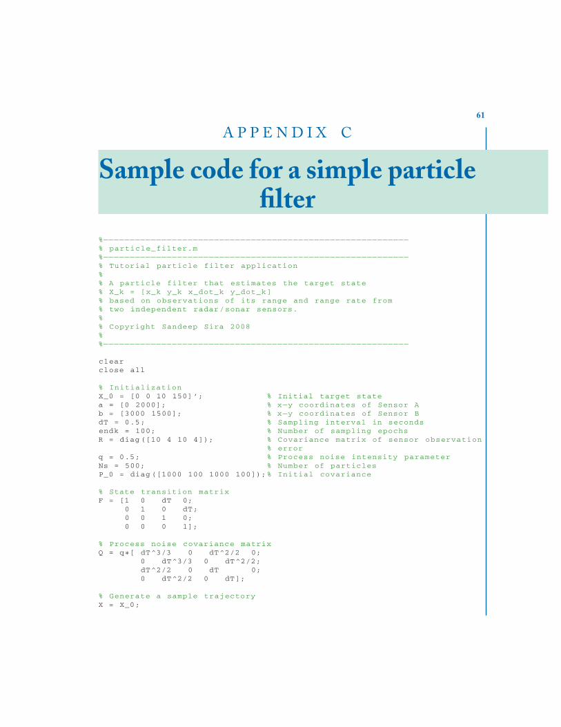
61

A P P E N D I X C

Sample code for a simple particlefilter

%−−−−−−−−−−−−−−−−−−−−−−−−−−−−−−−−−−−−−−−−−−−−−−−−−−−−−−−−−−% particle_filter.m%−−−−−−−−−−−−−−−−−−−−−−−−−−−−−−−−−−−−−−−−−−−−−−−−−−−−−−−−−−% Tutorial particle filter application%% A particle filter that estimates the target state% X_k = [x_k y_k x_dot_k y_dot_k]% based on observations of its range and range rate from% two independent radar/sonar sensors.%% Copyright Sandeep Sira 2008%%−−−−−−−−−−−−−−−−−−−−−−−−−−−−−−−−−−−−−−−−−−−−−−−−−−−−−−−−−−

clearclose all

% InitializationX_0 = [0 0 10 150] ’; % Initial target statea = [0 2000]; % x−y coordinates of Sensor Ab = [3000 1500]; % x−y coordinates of Sensor BdT = 0.5; % Sampling interval in secondsendk = 100; % Number of sampling epochsR = diag ([10 4 10 4]); % Covariance matrix of sensor observation

% errorq = 0.5; % Process noise intensity parameterNs = 500; % Number of particlesP_0 = diag ([1000 100 1000 100]);% Initial covariance

% State transition matrixF = [1 0 dT 0;

0 1 0 dT;0 0 1 0;0 0 0 1];

% Process noise covariance matrixQ = q ∗[ dT^3/3 0 dT^2/2 0;

0 dT^3/3 0 dT^2/2;dT^2/2 0 dT 0;0 dT^2/2 0 dT];

% Generate a sample trajectoryX = X_0;

62 APPENDIX C. SAMPLE CODE FOR A SIMPLE PARTICLE FILTER

sqrtm_Q = sqrtm(Q);for k = 2:endk

X(:,k) = F ∗X(:,k−1) + sqrtm_Q ∗ randn (4 ,1);end

% Sample an initial value of the target state.% This is the mean of the density P(X_0)XHat (:,1) = X_0 + sqrtm(P_0 )∗ randn (4 ,1);

% Sample the particles from the initial densityXp = XHat ∗ ones(1,Ns) + sqrtm(P_0 )∗ randn(4,Ns);

% Commence particle filtering loopsqrtm_R = sqrtm(R);inv_R = inv(R);for k = 2:endk

% Project the particles forward according to the target kinematics% modelXp = F ∗Xp + sqrtm_Q ∗ randn(4, Ns);

% Get the true observationzeta = X(:,k);% Range from Sensor Ada_true = norm( zeta ([1:2]) − a’);% Range from Sensor Bdb_true = norm( zeta ([1:2]) − b’);% Range−rate wrt Sensor Ava_true = zeta ([3:4]) ’ ∗ (zeta ([1:2]) − a’)/ da_true;% Range−rate wrt Sensor Bvb_true = zeta ([3:4]) ’ ∗ (zeta ([1:2]) − b’)/ db_true;

% Add the sensor noiseZk = [ da_true; va_true; db_true; vb_true] + sqrtm_R ∗ randn (4 ,1);

% Obtain the observations corresponding to each particleda = sqrt( sum( (Xp([1,2],:) − a ’∗ ones(1,Ns)).^ 2 ) );db = sqrt( sum( (Xp([1,2],:) − b ’∗ ones(1,Ns)).^ 2 ) );va = diag(Xp([3:4] ,:) ’ ∗ ( Xp([1:2] ,:) − a ’∗ ones(1,Ns)))’ ./ da;vb = diag(Xp([3:4] ,:) ’ ∗ ( Xp([1:2] ,:) − b ’∗ ones(1,Ns)))’ ./ db;

% Obtain a matrix of range and range−rates , one column per particleZ = [da; va; db; vb];

% Calculate the weightsinnov = Zk ∗ ones(1,Ns) − Z;

w = diag( exp(−0.5 ∗ innov ’ ∗ inv_R ∗ innov) )’;

% Normalize the weightsif sum(w) == 0

display(’Alarm weights = 0. Setting all weights equal!’)w = ones(1,Ns)/Ns;

endw = w / sum(w);

% Calculate the estimate

63

XHat(:,k) = Xp ∗w’;

% Plot the results so farfigure (1); clf;plot(X(1,:), X(2,:), ’b∗−’, XHat(1,:), XHat(2,:), ’co−’, ...

Xp(1,:), Xp(2,:), ’r.’);hold on%plot(a(1), a(2), ’rs ’, b(1), b(2), ’gs ’);title(’X−Y position ’); xlabel(’X (m)’); ylabel(’Y (m)’);legend(’Target trajectory ’, ’Target estimate ’, ...

’Particles ’, ’Location ’, ’SouthEast ’)

figure (2); clf;subplot (2,1,1),plot ([0:endk −1]∗dT, X(3,:), ’b∗−’, [0:k−1]∗dT, XHat(3,:), ...

’co−’, (k−1)∗dT ∗ ones(1,Ns), Xp(3,:), ’r.’);title(’Velocity ’); ylabel(’X m/s’);subplot (2,1,2),plot ([0:endk −1]∗dT, X(4,:), ’b∗−’, [0:k−1]∗dT, XHat(4,:), ...

’co−’, (k−1)∗dT ∗ ones(1,Ns), Xp(4,:), ’r.’);xlabel(’Sampling instant ’); ylabel(’Y m/s’);

% Resample the particles% ResampleXp = importance_resample(Xp, w);

end

% Plot the MSEfiguretrMSE = diag((XHat − X)’ ∗ (XHat − X));semilogy ([0:endk −1]∗dT , trMSE , ’b∗−’);xlabel(’Time’); ylabel(’MSE’);title(’Total Mean Square Tracking Error’);

% −−−−−−−−−−−−−−−−−−−−−−−−−−−−−−−−−−−−−−−−−−−−−−−−−−−−−−−−−−−−−−−−

function [Xpout , wout , index] = importance_resample(Xp, w)

% Carry out resampling.% Returns Particles , weights and index of parent of each particle

[a M] = size(Xp);

% Cumulative Distributive Functioncumpr = cumsum(w(1,1:M))’;cumpr = cumpr/max(cumpr);

u(1,1) = (1/M)∗ rand (1,1);i=1;for j = 1:M

u(j,1)= u(1,1) + (1/M)∗(j−1);while (u(j,1) > cumpr(i,1))

i = i+1;if i > M

break

64 APPENDIX C. SAMPLE CODE FOR A SIMPLE PARTICLE FILTER

endendif i ≤ M

x_update(:,j) = Xp(:,i);index(j) = i;

endend

Xpout = x_update;wout = 1/M ∗ ones(1,M);

return

65

A P P E N D I X D

Sample code for an unscentedparticle filter

%−−−−−−−−−−−−−−−−−−−−−−−−−−−−−−−−−−−−−−−−−−−−−−−−−−−−−−−−−−% unscented_particle_filter.m%−−−−−−−−−−−−−−−−−−−−−−−−−−−−−−−−−−−−−−−−−−−−−−−−−−−−−−−−−−% Unscented particle filter application%% A particle filter based on the unscented transform that% estimates the target state X_k = [x_k y_k x_dot_k y_dot_k]% based on observations of its range and range rate from% two independent radar/sonar sensors.%% Copyright Sandeep Sira 2008%%−−−−−−−−−−−−−−−−−−−−−−−−−−−−−−−−−−−−−−−−−−−−−−−−−−−−−−−−−−clearclose all

% InitializationX_0 = [0 0 10 150] ’; % Initial target statea = [0 2000]; % x−y coordinates of Sensor Ab = [3000 1500]; % x−y coordinates of Sensor BdT = 0.5; % Sampling interval in secondsendk = 100; % Number of sampling epochsR = diag ([10 4 10 4]); % Covariance matrix of sensor observation

% errorq = 0.5; % Process noise intensity parameterNs = 10; % Number of particlesP_0 = diag ([1000 100 1000 100]);% Initial covariance

% UPF parametersna = 4; kappa = 4; alpha = 1; beta = 0;lambda = alpha ^2∗( na+kappa) − na;

% State transition matrixF = [1 0 dT 0;

0 1 0 dT;0 0 1 0;0 0 0 1];

% Process noise covariance matrixQ = q ∗[ dT^3/3 0 dT^2/2 0;

0 dT^3/3 0 dT^2/2;dT^2/2 0 dT 0;0 dT^2/2 0 dT];

66 APPENDIX D. SAMPLE CODE FOR AN UNSCENTED PARTICLE FILTER

sqrtm_Q = sqrtm(Q);inv_Q = inv(Q);inv_R = inv(R);sqrtm_R = sqrtm(R);

% Generate a target trajectoryX = X_0;for k = 2:endk

X(:,k) = F ∗X(:,k−1) + sqrtm_Q ∗ randn (4 ,1);end

% Sample an initial value of the target state. This is the mean of the% density P(X_0)XHat (:,1) = X_0 + sqrtm(P_0 )∗ randn (4 ,1);

% Sample the particles from the initial densityXp = XHat ∗ ones(1,Ns) + sqrtm(P_0 )∗ randn(4,Ns);

% Mean and covariance of particlesmx = mean(Xp ,2)∗ ones(1,Ns); err_X = Xp − mx;for j = 1:Ns

P_xx(:,:,j) = err_X(:,j) ∗ err_X(:,j)’;end

% Commence unscented particle filtering loopfor k = 2:endk

% Project the particles forwardXp_in = F ∗Xp;

% Get the observationzeta = X(:,k);da_true = norm( zeta ([1:2]) − a’);db_true = norm( zeta ([1:2]) − b’);va_true = zeta ([3:4]) ’ ∗ (zeta ([1:2]) − a’)/ da_true;vb_true = zeta ([3:4]) ’ ∗ (zeta ([1:2]) − b’)/ db_true;Zk = [ da_true; va_true; db_true; vb_true] + sqrtm_R ∗ randn (4 ,1);

for j = 1:Ns

% Obtain the sigma pointsP(:,:) = P_xx(:,:,j);sqrt_P_xx = real(sqrtm( (na + lambda )∗P ));chi_X (:,:) = mx(:,j)∗ ones (1 ,2∗na+1) + ...

[ zeros (4,1) sqrt_P_xx −sqrt_P_xx ];w_chi = [ kappa ones (1 ,2∗na)/2 ] / (na + kappa);

% Propagate the sigma pointschi_X = F ∗ chi_X + sqrtm_Q ∗ randn (4 ,2∗na+1);

% Calculate mean and variancemx(:,j) = chi_X ∗ w_chi ’;err_chi_X = chi_X − mx(:,j)∗ ones (1 ,2∗na+1);PHat = err_chi_X ∗ (err_chi_X. ∗( ones (4 ,1)∗ w_chi))’;

% Range and range rate of the sigma points as

67

% observed by the sensorschi_X_da = sqrt( sum( (chi_X ([1,2],:) − a ’∗ ones (1,9)).^ 2 ) );chi_X_db = sqrt( sum( (chi_X ([1,2],:) − b ’∗ ones (1,9)).^ 2 ) );chi_X_va = diag(chi_X ([3:4] ,:) ’ ...

∗ ( chi_X ([1:2] ,:) − a ’∗ ones (1,9)))’ ./ chi_X_da;chi_X_vb = diag(chi_X ([3:4] ,:) ’ ...

∗ ( chi_X ([1:2] ,:) − b ’∗ ones (1,9)))’ ./ chi_X_db;

chi_Z = [chi_X_da; chi_X_va; chi_X_db; chi_X_vb ];m_chi_Z = chi_Z ∗ w_chi ’;err_chi_Z = chi_Z − m_chi_Z ∗ ones (1,9);

% Obtain P_zz , P_xzP_zz = zeros (4 ,4); P_xz = zeros (4 ,4);P_zz = err_chi_Z ∗ (err_chi_Z. ∗( ones (4 ,1)∗ w_chi))’;P_xz = err_chi_X ∗ (err_chi_Z. ∗( ones (4 ,1)∗ w_chi))’;

% Innovations covariance and Kalman gainP_eta = P_zz + R; K = P_xz ∗ inv(P_eta);

% Updatemx(:,j) = mx(:,j) + K ∗ (Zk − m_chi_Z );PHat = PHat − K ∗ P_eta ∗ K’;

% Store for the next time stepP_xx(:,:,j) = PHat;

% Sample a new particleXp(:,j) = mx(:,j) + real(sqrtm(PHat ))∗ randn (4 ,1);

% Importance density component of the weightw3(j) = exp(−0.5 ∗ ( Xp(:,j) − mx(:,j) )’ ...

∗ inv(PHat) ∗ ( Xp(:,j) − mx(:,j) ) );

end

% Calculate the weightsda = sqrt( sum( (Xp([1:2] ,:) − a ’∗ ones(1,Ns)).^2 ));db = sqrt( sum( (Xp([1:2] ,:) − b ’∗ ones(1,Ns)).^2 ));va = diag(Xp([3:4] ,:) ’ ∗ ( Xp([1:2] ,:) − a ’∗ ones(1,Ns)))’ ./ da;vb = diag(Xp([3:4] ,:) ’ ∗ ( Xp([1:2] ,:) − b ’∗ ones(1,Ns)))’ ./ db;

innov = Zk ∗ ones(1,Ns) − [ da; va; db; vb];

% Likelihood componentw1 = diag( exp(−0.5 ∗ innov ’ ∗ inv_R ∗ innov) )’;% Kinematic prior componentw2 = diag( exp(−0.5 ∗ ( Xp − Xp_in )’ ∗ inv_Q ∗ ...

( Xp − Xp_in ) ) )’;

w = w1 . ∗ w2 ./ w3;

if sum(w) == 0fprintf(’Alarm weights = 0 at time step %d\n’, k);w = ones(1,Ns)/Ns;

end

68 APPENDIX D. SAMPLE CODE FOR AN UNSCENTED PARTICLE FILTER

w = w / sum(w);

N_eff = 1 / (w ∗ w’);

% Calculate the estimateXHat(:,k) = Xp ∗w’;

% Plot the results so farfigure (1); clf;plot(X(1,:), X(2,:), ’b∗−’, XHat(1,:), XHat(2,:), ’co−’, ...

Xp(1,:), Xp(2,:), ’r.’);hold on%plot(a(1), a(2), ’rs ’, b(1), b(2), ’gs ’);title(’X−Y position ’); xlabel(’X (m)’); ylabel(’Y (m)’);legend(’Target trajectory ’, ’Target estimate ’, ...

’Particles ’, ’Location ’, ’SouthEast ’)

figure (2); clf;subplot (2,1,1),plot ([0:endk −1]∗dT, X(3,:), ’b∗−’, [0:k−1]∗dT, XHat(3,:), ...

’co−’, (k−1)∗dT ∗ ones(1,Ns), Xp(3,:), ’r.’);title(’Velocity ’); ylabel(’X m/s’);subplot (2,1,2),plot ([0:endk −1]∗dT, X(4,:), ’b∗−’, [0:k−1]∗dT, XHat(4,:), ...

’co−’, (k−1)∗dT ∗ ones(1,Ns), Xp(4,:), ’r.’);xlabel(’Sampling instant ’); ylabel(’Y m/s’);

% Resample[Xp w index] = importance_resample(Xp, w);

% Housekeepingmx = mx(:,index);P_xx = P_xx(:,:,index );

end

fprintf(’\n\n’);

% Plot the MSEfiguretrMSE = diag((XHat − X)’ ∗ (XHat − X));semilogy ([0:endk −1]∗dT , trMSE , ’b∗−’);xlabel(’Time’); ylabel(’MSE’);title(’Total Mean Square Tracking Error’);

69

Bibliography

[1] A. Drozd, “Waveform diversity and design,” IEEE EMC Society Newsletter, Summer 2006.[Online]. Available:http://www.ieee.org/organizations/pubs/newsletters/emcs/summer06/cover_story.pdf

[2] D. Cochran, “Reducing complexity for defense,” DARPATech 2002 Symposium, Jul. 2002.[Online]. Available:http://web-ext2.darpa.mil/DARPATech2002/presentations/dso_pdf/speeches/COCHRAN.pdf

[3] Y. Bar-Shalom and T. E. Fortmann, Tracking and Data Association. Boston: AcademicPress, 1988.

[4] R. L. Mitchell and A. W. Rihaczek, “Matched filter responses of the linear FM waveform,”IEEE Trans. Aerosp. Electron. Syst., vol. 4, pp. 417–432, May 1968.

[5] D. F. DeLong and E. M. Hofstetter, “On the design of optimum radar waveforms forclutter rejection,” IEEE Trans. Inform. Theory, vol. IT-13, no. 3, pp. 454–463, Jul. 1967.DOI: 10.1109/TIT.1967.1054038

[6] R. McAulay and J. Johnson, “Optimal mismatched filter design for radar ranging, de-tection, and resolution,” IEEE Trans. Inform. Theory, vol. 17, pp. 696–701, Nov. 1971.DOI: 10.1109/TIT.1971.1054722

[7] M.Athans and F.C.Schweppe,“Optimal waveform design via control theoretic principles,” In-formation and Control, vol.10,pp.335–377,Apr.1967.DOI: 10.1016/S0019-9958(67)90183-0

[8] F. C. Schweppe and D. L. Gray, “Radar signal design subject to simultaneous peak andaverage power constraints,” IEEE Trans. Inform. Theory, vol. IT-12, pp. 13–26, Jan. 1966.DOI: 10.1109/TIT.1966.1053853

[9] M. R. Bell, “Information theory and radar waveform design,” IEEE Trans. Inform. Theory,vol. 39, pp. 1578–1597, Sep. 1993. DOI: 10.1109/18.259642

[10] K.T. Wong, “Adaptive pulse-diverse radar/sonar waveform design,” in IEEE Radar Conference,pp. 105–110, May 1998. DOI: 10.1109/NRC.1998.677985

http://www.ieee.org/organizations/pubs/newsletters/emcs/summer06/

cover_story.pdf

http://web-ext2.darpa.mil/DARPATech2002/presentations/dso_pdf/speeches/

COCHRAN.pdf

http://dx.doi.org/10.1109/TIT.1967.1054038


http://dx.doi.org/10.1016/S0019-9958(67)90183-0


http://dx.doi.org/10.1109/18.259642

http://dx.doi.org/10.1109/NRC.1998.677985

70 BIBLIOGRAPHY

[11] N. Wang, Y. Zhang, and S. Wu, “Radar waveform design and target detection us-ing wavelets,” in CIE International Conference on Radar, pp. 506–509, Oct. 2001.DOI: 10.1109/ICR.2001.984758

[12] R. J. Bonneau, “A wavelet packet basis optimization approach to radar waveform design,” inIEEE International Symposium on Antennas and Propagation, vol. 4, pp. 814–816, Jul. 2001.DOI: 10.1109/APS.2001.959589

[13] S. M. Sowelam and A. H. Tewfik, “Waveform selection in radar target classification,” IEEETrans. Inform. Theory, vol. 46, pp. 1014–1029, May 2000. DOI: 10.1109/18.841178

[14] D. Garren, M. Osborn, A. Odom, J. Goldstein, S. Pillai, and J. Guerci, “Enhanced target detec-tion and identification via optimised radar transmission pulse shape,” IEE Proceedings-RadarSonar and Navigation, vol. 148, no. 3, pp. 130–138, 2001. DOI: 10.1049/ip-rsn:20010324

[15] S.-M. Hong, R. J. Evans, and H.-S. Shin, “Control of waveforms and detection thresholds foroptimal target tracking in clutter,” in Proceedings of the 39th IEEE Conference on Decision andControl, vol. 4, pp. 3906–3907, Dec. 2000. DOI: 10.1109/CDC.2000.912323

[16] S.-M. Hong, R. J. Evans, and H.-S. Shin, “Optimization of waveform and detection thresholdfor target tracking in clutter,” in Proceedings of the 40th SICE Annual Conference, pp. 42–47, Jul.2005. DOI: 10.1109/SICE.2001.977803

[17] D. J. Kershaw and R. J. Evans, “Optimal waveform selection for tracking systems,” IEEE Trans.Inform. Theory, vol. 40, no. 5, pp. 1536–1550, Sep. 1994. DOI: 10.1109/18.333866

[18] D. J. Kershaw and R. J. Evans, “Waveform selective probabilistic data association,” IEEE Trans.Aerosp. Electron. Syst., vol. 33, pp. 1180–1188, Oct. 1997. DOI: 10.1109/7.625110

[19] C. Rago, P. Willett, and Y. Bar-Shalom, “Detection-tracking performance with com-bined waveforms,” IEEE Trans. Aerosp. Electron. Syst., vol. 34, pp. 612–624, Apr. 1998.DOI: 10.1109/7.670395

[20] R. Niu, P. Willett, and Y. Bar-Shalom, “Tracking considerations in selection of radar waveformfor range and range-rate measurements,” IEEE Trans. Aerosp. Electron. Syst., vol. 38, no. 2, pp.467–487, Apr. 2002. DOI: 10.1109/TAES.2002.1008980

[21] S. D. Howard, S. Suvorova, and W. Moran, “Waveform libraries for radar tracking applica-tions,” International Conference on Waveform Diversity and Design, Edinburgh, UK, Nov. 2004.DOI: 10.1109/CISS.2006.286688

[22] S.P.Sira,A.Papandreou-Suppappola, and D.Morrell,“Dynamic configuration of time-varyingwaveforms for agile sensing and tracking in clutter,” IEEETrans. Signal Processing, vol. 55,no.1,pp. 3207–3217, Jun. 2007. DOI: 10.1109/TSP.2007.894418

http://dx.doi.org/10.1109/ICR.2001.984758

http://dx.doi.org/10.1109/APS.2001.959589

http://dx.doi.org/10.1109/18.841178

http://dx.doi.org/10.1049/ip-rsn:20010324

http://dx.doi.org/10.1109/CDC.2000.912323

http://dx.doi.org/10.1109/SICE.2001.977803

http://dx.doi.org/10.1109/18.333866

http://dx.doi.org/10.1109/7.625110

http://dx.doi.org/10.1109/7.670395

http://dx.doi.org/10.1109/TAES.2002.1008980

http://dx.doi.org/10.1109/CISS.2006.286688

http://dx.doi.org/10.1109/TSP.2007.894418

BIBLIOGRAPHY 71

[23] S. M. Hong, R. J. Evans, and H. S. Shin, “Optimization of waveform and detection thresholdfor range and range-rate tracking in clutter,” IEEE Trans. Aerosp. Electron. Syst., vol. 41, no. 1,pp. 17–33, Jan. 2005. DOI: 10.1109/TAES.2005.1413743

[24] B. F. L. Scala, W. Moran, and R. J. Evans, “Optimal adaptive waveform selec-tion for target detection,” in International Conference on Radar, pp. 492–496, 2003.DOI: 10.1109/RADAR.2003.1278791

[25] A. Doucet, N. de Freitas, and N. Gordon, Eds., Sequential Monte Carlo Methods in Practice.Springer-Verlag, 2001.

[26] M. S. Arulampalam, S. Maskell, N. Gordon, and T. Clapp, “A tutorial on particle filters foronline nonlinear/non-Gaussian Bayesian tracking,” IEEE Trans. Signal Processing, vol. 50, pp.174–188, Feb. 2002. DOI: 10.1109/78.978374

[27] E.Kalman,Rudolph,“A new approach to linear filtering and prediction problems,” Transactionsof the ASME–Journal of Basic Engineering, vol. 82, no. Series D, pp. 35–45, 1960.

[28] R. van der Merwe, N. de Freitas, A. Doucet, and E. Wan, “The Unscented Particle Filter,” inAdvances in Neural Information Processing Systems 13, Nov. 2001.

[29] S. Julier and J. Uhlmann, “A new extension of the Kalman filter to nonlinear sys-tems,” International Symposium on Aerospace/Defense Sensing, Simulation and Controls, 1997.DOI: 10.1117/12.280797

[30] L. J. Ziomek, Underwater Acoustics: A Linear Systems Theory Approach.Orlando, FL: AcademicPress, 1985.

[31] R. O. Nielsen, Sonar Signal Processing. Artech House, 1991.

[32] M. I. Skolnik, Radar Handbook, 2nd ed., M. I. Skolnik, Ed. New York: McGraw Hill, 1990.

[33] A. Papandreou-Suppappola, R. L. Murray, B. G. Iem, and G. F. Boudreaux-Bartels, “Groupdelay shift covariant quadratic time-frequency representations,” IEEE Trans. Signal Processing,vol. 49, pp. 2549–2564, 2001. DOI: 10.1109/78.960403

[34] A. Papandreou-Suppappola, Time-Varying Processing: Tutorial on Principles and Practice inApplications in Time-Frequency Signal Processing, A. Papandreou-Suppappola, Ed. Florida:CRC Press, 2002.

[35] R. A. Altes and E. L.Titlebaum,“Bat signals as optimally Doppler tolerant waveforms,” Journalof the Acoustical Society of America, vol. 48, pp. 1014–1020, Oct. 1970. DOI: 10.1121/1.1912222

[36] H. L. Van Trees, Detection Estimation and Modulation Theory, Part III. New York: Wiley, 1971.


http://dx.doi.org/10.1109/RADAR.2003.1278791

http://dx.doi.org/10.1109/78.978374

http://dx.doi.org/10.1117/12.280797

http://dx.doi.org/10.1109/78.960403

http://dx.doi.org/10.1121/1.1912222

72 BIBLIOGRAPHY

[37] L. G. Weiss, “Wavelets and wideband correlation processing,” IEEE Signal Processing Mag.,pp. 13–32, Jan. 1994. DOI: 10.1109/79.252866

[38] L. Cohen, Time-Frequency Analysis. Englewood Cliffs, New Jersey: Prentice-Hall, 1995.

[39] D. W. Ricker, Echo Signal Processing. Kluwer Academic Publishers, 2003.

[40] P. L’Ecuyer, “An overview of derivative estimation,” Proceedings of the 1991 Winter SimulationConference, pp. 207–217, Dec. 1991. DOI: 10.1109/WSC.1991.185617

[41] G. Pflug, Optimization of Stochastic Models: The Interface Between Simulation and Optimization.Kluwer Academic Publishers, 1996.

[42] J. C. Spall, “Multivariate stochastic approximation using a simultaneous perturbation gra-dient approximation,” IEEE Trans. Automat. Contr., vol. 37, pp. 332–341, Mar. 1992.DOI: 10.1109/9.119632

[43] J. Kiefer and J. Wolfowitz, “Stochastic estimation of a regression function,” Annals of Mathe-matical Statistics, vol. 23, pp. 462–466, Sep. 1952. DOI: 10.1214/aoms/1177729392

[44] P. Sadegh and J. C. Spall, “Constrained optimization via stochastic approximation with a simul-taneous perturbation gradient approximation,” Automatica, vol. 33, no. 5, pp. 889–892, 1997.DOI: 10.1016/S0005-1098(96)00230-0

[45] S. P. Sira, D. Morrell, and A. Papandreou-Suppappola, “Waveform design and scheduling foragile sensors for target tracking,” Asilomar Conference on Signals, Systems and Computers, vol. 1,pp. 820–824, Nov. 2004. DOI: 10.1109/ACSSC.2004.1399251

[46] B. D. Anderson and J. B. Moore, Optimal Filtering. New Jersey: Prentice-Hall, 1979.

[47] S. P. Sira, A. Papandreou-Suppappola, and D. Morrell, “Time-varying waveform selec-tion and configuration for agile sensors in tracking applications,” IEEE InternationalConference on Acoustics, Speech, and Signal Processing, vol. 5, pp. 881–884, Mar. 2005.DOI: 10.1109/ICASSP.2005.1416445

[48] D. A. Swick, “A review of wideband ambiguity functions,” Naval Research Laboratory, Wash-ington, D.C., Tech. Rep. 6994, Dec. 1969.

[49] Q. Jin, K. M. Wong, and Z.-Q. Luo, “The estimation of time delay and doppler stretchof wideband signals,” IEEE Trans. Signal Processing, vol. 43, no. 4, pp. 904–916, Apr. 1995.DOI: 10.1109/78.376843

[50] Y. Doisy, L. Deruaz, S. P. Beerens, and R. Been, “Target doppler estimation using widebandfrequency modulated signals,” IEEE Trans. Signal Processing, vol. 48, no. 5, pp. 1213–1224,May 2000. DOI: 10.1109/78.839970

http://dx.doi.org/10.1109/79.252866

http://dx.doi.org/10.1109/WSC.1991.185617

http://dx.doi.org/10.1109/9.119632

http://dx.doi.org/10.1214/aoms/1177729392

http://dx.doi.org/10.1016/S0005-1098(96)00230-0

http://dx.doi.org/10.1109/ACSSC.2004.1399251

http://dx.doi.org/10.1109/ICASSP.2005.1416445

http://dx.doi.org/10.1109/78.376843

http://dx.doi.org/10.1109/78.839970

BIBLIOGRAPHY 73

[51] C. E. Cook and M. Bernfeld, Radar Signals, An Introduction to Theory and Application. Boston:Artech House, 1993.

[52] S. P. Sira, A. Papandreou-Suppappola, and D. Morrell, “Waveform scheduling in widebandenvironments,” IEEE International Conference on Acoustics, Speech, and Signal Processing, vol. 1,pp. I–697 – I–700, May 2006. DOI: 10.1109/ICASSP.2006.1661477

[53] S. P. Sira, A. Papandreou-Suppappola, and D. Morrell, “Characterization of waveform perfor-mance in clutter for dynamically configured sensor systems,” Waveform Diversity and DesignConference, Lihue, Hawaii, Jan. 2006.

[54] R. Niu, P. Willett, and Y. Bar-Shalom, “Matrix CRLB scaling due to measurements ofuncertain origin,” IEEE Trans. Signal Processing, vol. 49, no. 7, pp. 1325–1335, Jul. 2001.DOI: 10.1109/78.928687

[55] T. Fortmann, Y. Bar-Shalom, M. Scheffe, and S. Gelfand, “Detection thresholds for trackingin clutter - A connection between estimation and signal processing,” IEEE Trans. Automat.Contr., vol. 30, pp. 221–229, Mar. 1985. DOI: 10.1109/TAC.1985.1103935

[56] D. J. Kershaw and R. J. Evans, “A contribution to performance prediction for probabilistic dataassociation tracking filters,” IEEE Trans. Aerosp. Electron. Syst., vol. 32, no. 3, pp. 1143–1147,Jul. 1996. DOI: 10.1109/7.532274

[57] S. P. Sira, A. Papandreou-Suppappola, and D. Morrell, “Waveform-agile sensing for trackingmultiple targets in clutter,” Conference on Information Sciences and Systems, Princeton, NJ, pp.1418–1423, Mar. 2006. DOI: 10.1109/CISS.2006.286687

[58] C. Kreucher, K. Kastella, and Alfred O. Hero, III, “Multitarget tracking using the joint mul-titarget probability density,” IEEE Trans. Aerosp. Electron. Syst., vol. 41, no. 4, pp. 1396–1414,Oct. 2005. DOI: 10.1109/TAES.2005.1561892

[59] J. A. Simmons and R. Stein, “Acoustic imaging in bat sonar: Echolocation signals and theevolution of echolocation,” Journal of Comparative Psychology, vol. 135, no. 1, pp. 61–84, Mar.1980. DOI: 10.1007/BF00660182

[60] J. A. Simmons, P. A. Saillant, and S. P. Dear, “Through a bat’s ear,” IEEE Spectrum, vol. 29, pp.46–48, Mar. 1992. DOI: 10.1109/6.123330

http://dx.doi.org/10.1109/ICASSP.2006.1661477

http://dx.doi.org/10.1109/78.928687

http://dx.doi.org/10.1109/TAC.1985.1103935

http://dx.doi.org/10.1109/7.532274

http://dx.doi.org/10.1109/CISS.2006.286687


http://dx.doi.org/10.1007/BF00660182

http://dx.doi.org/10.1109/6.123330

74

BiographySandeep P. Sira received the M.Tech.degree from the Indian Institute ofTechnology,Kanpur,

India, in 1999, and the Ph.D. degree in electrical engineering in 2007 from Arizona State Univer-sity (ASU). In 2007, he was a post-doctoral research associate at ASU. He is currently with ZoundsInc., in Mesa, Arizona. His research interests include waveform-agile sensing, target tracking, audiosignal processing, and detection and estimation theory.

Antonia Papandreou-Suppappola is a Professor in the Department of Electrical Engineer-ing at Arizona State University (ASU). She is the co-Director of the Sensor, Signal and InformationProcessing (SenSIP) Center, and Associate Director of the Adaptive Intelligent Materials and Sys-tems (AIMS) Center at ASU. Her research interests are in the areas of Waveform-Agile Sensing,Time-Frequency Signal Processing, and Statistical Signal Processing. She is currently funded by anAir Force Office of Scientific Research (AFOSR) Multidisciplinary University Research Initiative(MURI) on Adaptive Waveform Design for Full Spectral Dominance, and she participated in theDARPA Waveform-Agile Sensing, program, where she worked on waveform selection algorithmsfor sensing in highly cluttered environments.

Darryl Morrell is an associate professor of engineering at Arizona State University, wherehe is participating in the design and implementation of a multidisciplinary undergraduate engineer-ing program using innovative, research-based pedagogical and curricular approaches. His researchinterests include stochastic decision theory applied to sensor scheduling and information fusion aswell as application of research-based pedagogy to engineering education.

advances in waveform agile sensing for tracking

Documents

agile tracking

dynamic waveform selection

active sensing

azsynthesis lectures

viicontentssynthesis

review of recent advances

tracking problem formulation

thedesign of waveforms