advantages of a wholly bayesian approach to assessing
TRANSCRIPT

0
Advantages of a wholly Bayesian approach
to assessing efficacy in early drug
development: a case study
Phil Woodward, Ros Walley, Claire Birch, Jem Gale
Outline
• Background
• Prior information
• Decision criteria
• Theory: normal prior with normal likelihood
• Assessment of study design
Approximate posterior distribution for treatment effect
Design characteristics
Impact of study design on beliefs as to treatment effect
• Interim analysis
• Interactions with ethics boards and regulators
• Conclusions
Can we make better decisions using informative treatment priors?
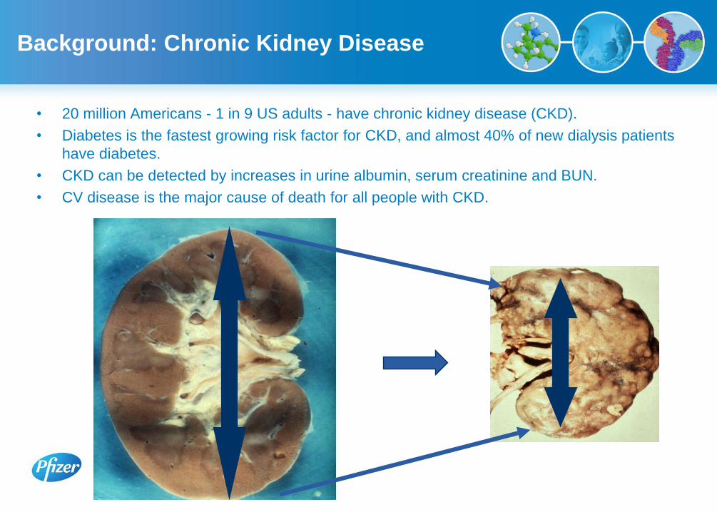
Background: Chronic Kidney Disease
• 20 million Americans - 1 in 9 US adults - have chronic kidney disease (CKD).
• Diabetes is the fastest growing risk factor for CKD, and almost 40% of new dialysis patients
have diabetes.
• CKD can be detected by increases in urine albumin, serum creatinine and BUN.
• CV disease is the major cause of death for all people with CKD.
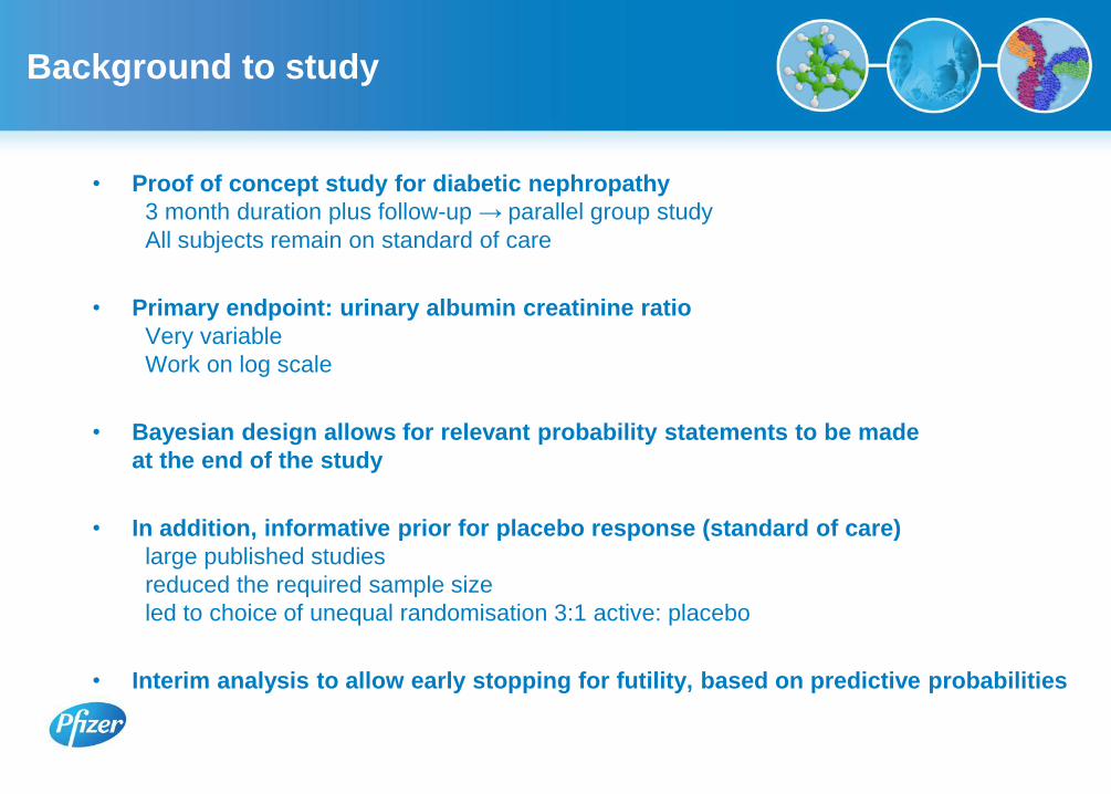
Background to study
• Proof of concept study for diabetic nephropathy
3 month duration plus follow-up → parallel group study
All subjects remain on standard of care
• Primary endpoint: urinary albumin creatinine ratio
Very variable
Work on log scale
• Bayesian design allows for relevant probability statements to be made
at the end of the study
• In addition, informative prior for placebo response (standard of care)
large published studies
reduced the required sample size
led to choice of unequal randomisation 3:1 active: placebo
• Interim analysis to allow early stopping for futility, based on predictive probabilities

Prior information
• Two uses of priors:
Design priors
to assess the study design only e.g. unconditional probability of success
Analysis priors
for use in analysis of the data (should be included in assessment of design)
• In this example,
Design priors: treatment effect and variance
Analysis prior: placebo response
• Found from
Published studies and internal data
Eliciting views from experts
• Sensitivity to priors will be assessed
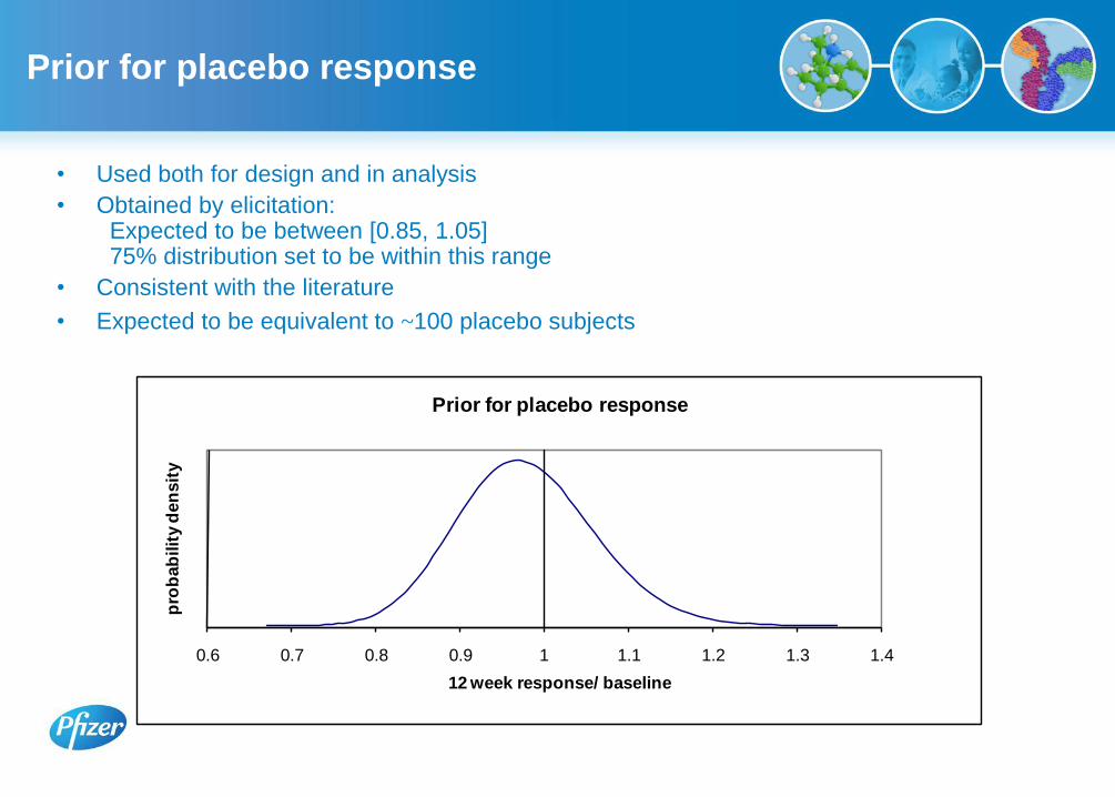
Prior for placebo response
• Used both for design and in analysis
• Obtained by elicitation: Expected to be between [0.85, 1.05] 75% distribution set to be within this range
• Consistent with the literature
• Expected to be equivalent to ~100 placebo subjects
0.6 0.7 0.8 0.9 1 1.1 1.2 1.3 1.4
pro
bab
ilit
y d
en
sit
y
12 week response/ baseline
Prior for placebo response
6
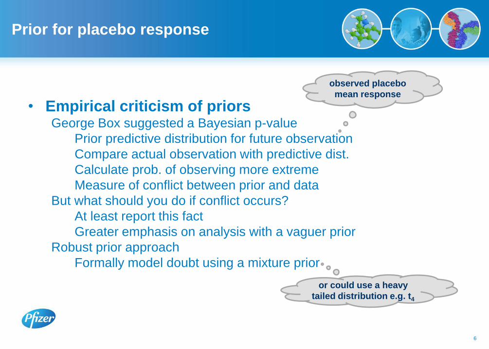
• Empirical criticism of priors George Box suggested a Bayesian p-value
Prior predictive distribution for future observation
Compare actual observation with predictive dist.
Calculate prob. of observing more extreme
Measure of conflict between prior and data
But what should you do if conflict occurs?
At least report this fact
Greater emphasis on analysis with a vaguer prior
Robust prior approach
Formally model doubt using a mixture prior
observed placebo
mean response
or could use a heavy
tailed distribution e.g. t4
Prior for placebo response
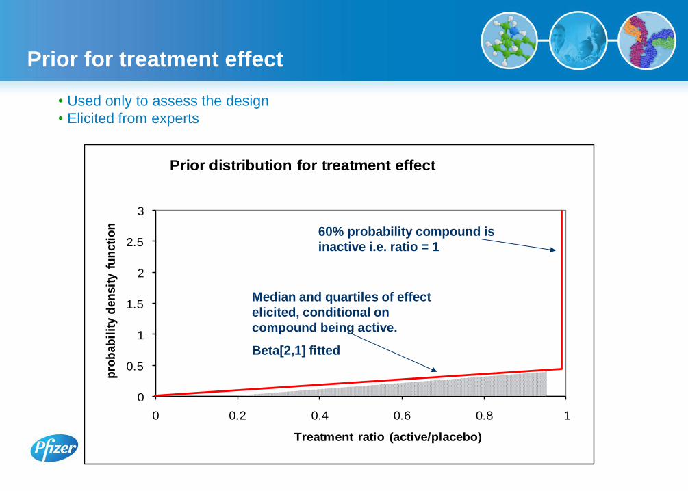
Prior for treatment effect
• Used only to assess the design
• Elicited from experts
0
0.5
1
1.5
2
2.5
3
0 0.2 0.4 0.6 0.8 1
pro
bab
ilit
y d
en
sit
y f
un
cti
on
Treatment ratio (active/placebo)
Prior distribution for treatment effect
60% probability compound is
inactive i.e. ratio = 1
Median and quartiles of effect
elicited, conditional on
compound being active.
Beta[2,1] fitted

Decision criteria
• In terms of 12 week data:
Criterion 1. At least 90% sure that the treatment ratio (active/placebo) < 1
Criterion 2. At least 67% sure the treatment ratio < 0.8
• In terms of n-fold reduction from baseline data:
Using the following notation for the posterior estimates on the log scale:
δ treatment difference, calculated as
– log(active) – log(placebo)
μδ posterior mean for δ
σδ posterior standard deviation of δ
T1= μδ – z0.9 .σδ; Criterion 1. T1 > 0
T2= μδ – z0.67 . σδ ; Criterion 2. T2 > -ln(0.8) = 0.22
Will revisit these statements
in light of using “flat” analysis prior
for treatment effect
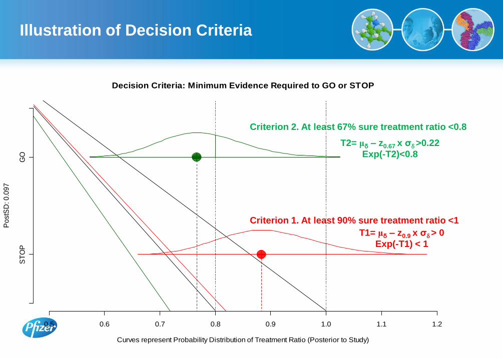
Illustration of Decision Criteria
Decision Criteria: Minimum Evidence Required to GO or STOP
Curves represent Probability Distribution of Treatment Ratio (Posterior to Study)
Po
stS
D: 0
.09
7
ST
OP
GO
0.5 0.6 0.7 0.8 0.9 1.0 1.1 1.2
Criterion 1. At least 90% sure treatment ratio <1
Criterion 2. At least 67% sure treatment ratio <0.8
T1= μδ – z0.9 x σδ > 0
Exp(-T1) < 1
T2= μδ – z0.67 x σδ >0.22
Exp(-T2)<0.8
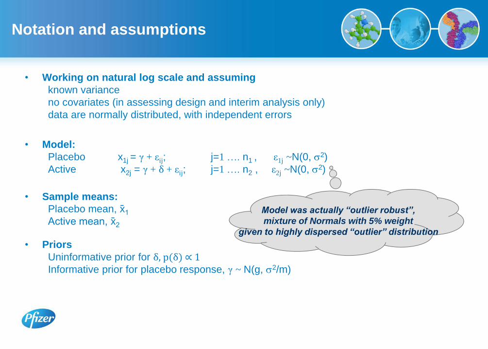
Notation and assumptions
• Working on natural log scale and assuming
known variance
no covariates (in assessing design and interim analysis only)
data are normally distributed, with independent errors
• Model:
Placebo x1j = γ + εij; j=1 …. n1 , ε1j ~N(0, 2)
Active x2j = γ + δ + εij; j=1 …. n2 , ε2j ~N(0, 2)
• Sample means:
Placebo mean, x1 Active mean, x2
• Priors
Uninformative prior for δ, p(δ) ∝ 1 Informative prior for placebo response, γ ~ N(g, 2/m)
Model was actually “outlier robust”,
mixture of Normals with 5% weight
given to highly dispersed “outlier” distribution

21
2
2
1
21
2
1
2
2
11
1
n
g
xn
nx
Posterior distribution for δ
• Posterior distribution for δ: normally distributed with
mean and variance
• Change notation for variance of prior for mean from 2/m to ω2
• Mean for posterior distribution for δ can be expressed
21
2
1
2
1
2
2
nm
n
x
m
g
x
1
21
22
2
nmn
k2 k1
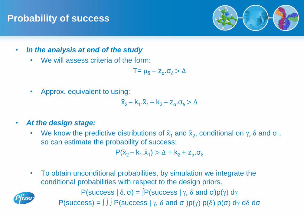
Probability of success
• In the analysis at end of the study
• We will assess criteria of the form:
T= μδ – zα.σδ > Δ
• Approx. equivalent to using:
x2 – k1.x1 – k2 – zα.σδ > Δ
• At the design stage:
• We know the predictive distributions of x1 and x2, conditional on γ, δ and σ ,
so can estimate the probability of success:
P(x2 – k1.x1) > Δ + k2 + zα.σδ
• To obtain unconditional probabilities, by simulation we integrate the
conditional probabilities with respect to the design priors.
P(success | δ, σ) = ∫P(success | γ, δ and σ)p(γ) dγ
P(success) = ∫ ∫ ∫ P(success | γ, δ and σ )p(γ) p(δ) p(σ) dγ dδ dσ
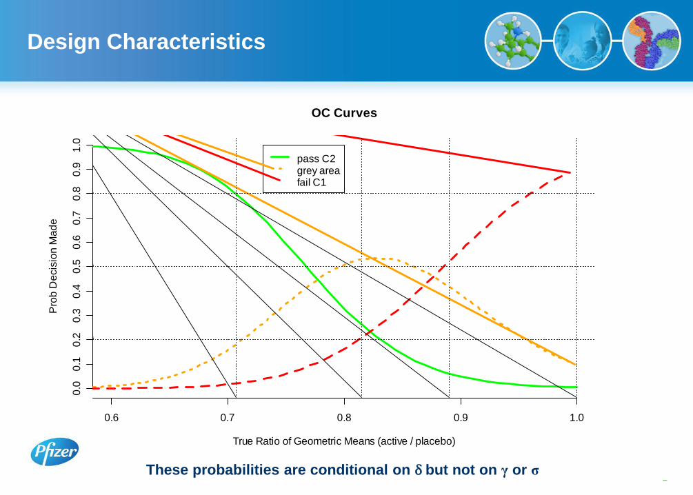
Design Characteristics
–13 These probabilities are conditional on δ but not on γ or σ
OC Curves
True Ratio of Geometric Means (active / placebo)
Pro
b D
ecis
ion
Ma
de
0.6 0.7 0.8 0.9 1.0
0.0
0.1
0.2
0.3
0.4
0.5
0.6
0.7
0.8
0.9
1.0
pass C2grey areafail C1
14
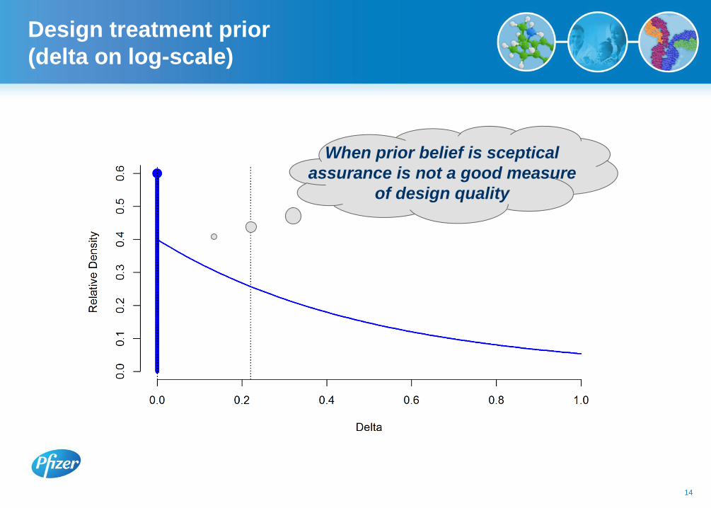
Design treatment prior
(delta on log-scale)
When prior belief is sceptical
assurance is not a good measure
of design quality
15
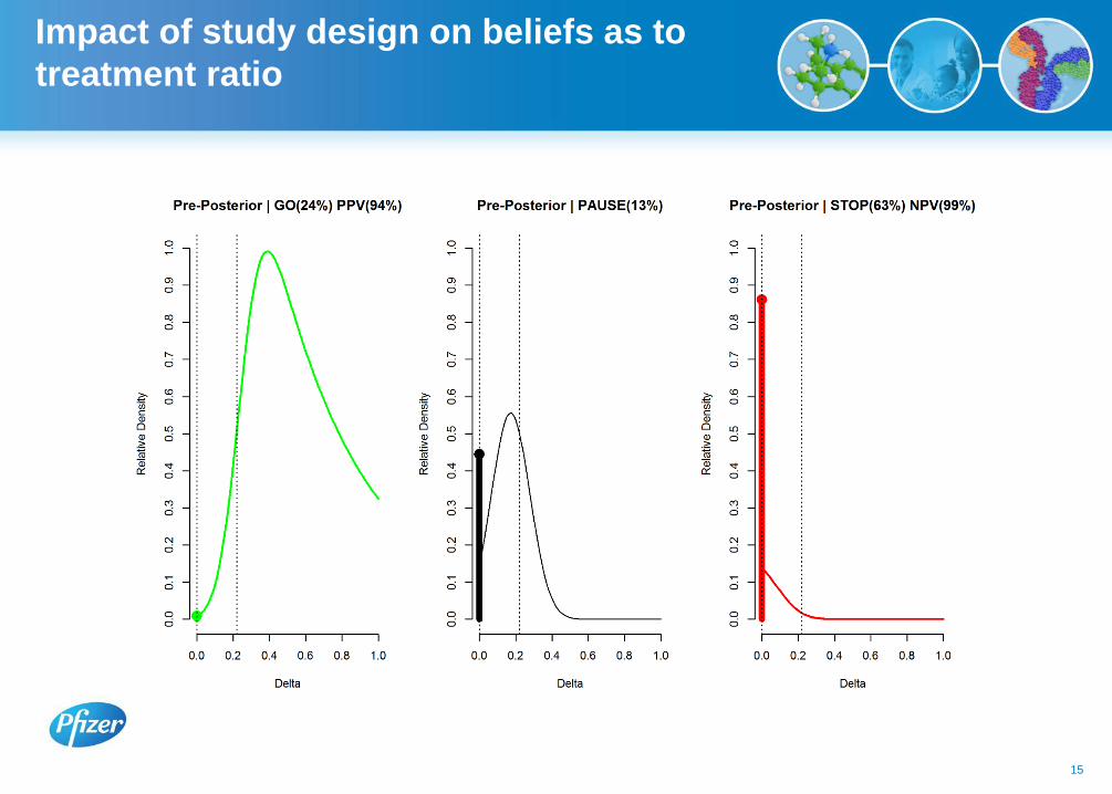
Impact of study design on beliefs as to
treatment ratio

Interim Analysis
• Proposal: To carry out an internal analysis when 25% subjects have completed, analysing end of treatment data
• Stopping rule: Stop at interim if the predictive probability of passing criterion 1 (lower hurdle) is less than 20%
• Potential saving: At the end of the interim, we estimate there will be 50 subjects left to recruit
• Implication: If stop decision at interim, small probability after all subjects have completed that we will just pass criterion 1.
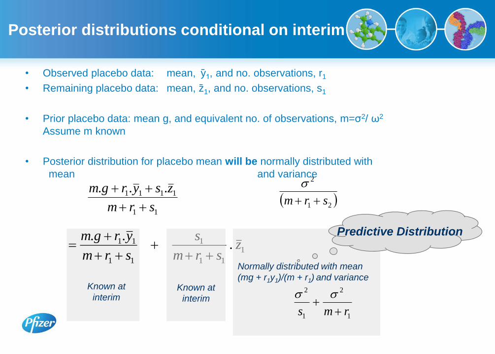
• Observed placebo data: mean, y1, and no. observations, r1
• Remaining placebo data: mean, z 1, and no. observations, s1
• Prior placebo data: mean g, and equivalent no. of observations, m=σ2/ ω2
Assume m known
• Posterior distribution for placebo mean will be normally distributed with
mean and variance
k1
Posterior distributions conditional on interim
11
1111 ...
srm
zsyrgm
21
2
srm
Known at
interim
1
11
1
11
11 ...
zsrm
s
srm
yrgm
Known at
interim
Normally distributed with mean
(mg + r1y1)/(m + r1) and variance
1
2
1
2
rms
Predictive Distribution

Assessing probability of success at interim
• Similarly can construct a posterior distribution for the active mean conditional on
the data.
• Recall at the end of the study we will assess criteria of the form:
T= μδ – zα.σδ > Δ
• From the joint distribution of these means we can compute the predictive
distribution for the treatment difference, δ, conditional on the interim data, and
thus calculate the probability this criterion will be satisfied

Probability of Stopping at Interim
True Value of Treatment Ratio (active/placebo)
Pro
ba
bility
Probability of stopping at interim
0.4 0.5 0.6 0.7 0.8 0.9 1.0
0.0
0.2
0.4
0.6
0.8
1.0

Interactions with Ethics Boards
and Regulators
• Non-standard approach → anticipate additional questions as well as standard ones e.g. method of randomisation
• No need to panic! Problem with translation More information → informed view No delay over and above other questions
• Lack of understanding versus wanting more detail e.g. functional forms of priors
• Whole power curve versus power at minimally clinically relevant difference
• Analogy with frequentist approach
• Level of detail No need to include priors that are used just to assess the design and give
unconditional probabilities of success

Small p-values are interpreted as evidence of real effect
But how much confidence do they provide in ED studies?
Are statements like “90% confidence effect > 0”
understood?
Does it matter?
Bayesian thinking
confidence is not “chance”
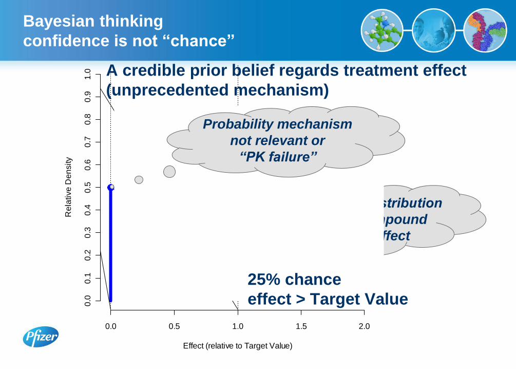
Bayesian thinking
confidence is not “chance”
A credible prior belief regards treatment effect
(unprecedented mechanism)
Prior “Belief” Distribution
assuming compound
has some effect
Effect (relative to Target Value)
Re
lative
De
nsity
0.0 0.5 1.0 1.5 2.0
0.0
0.1
0.2
0.3
0.4
0.5
0.6
0.7
0.8
0.9
1.0
Probability mechanism
not relevant or
“PK failure”
25% chance
effect > Target Value
mu
rela
tive
de
nsity
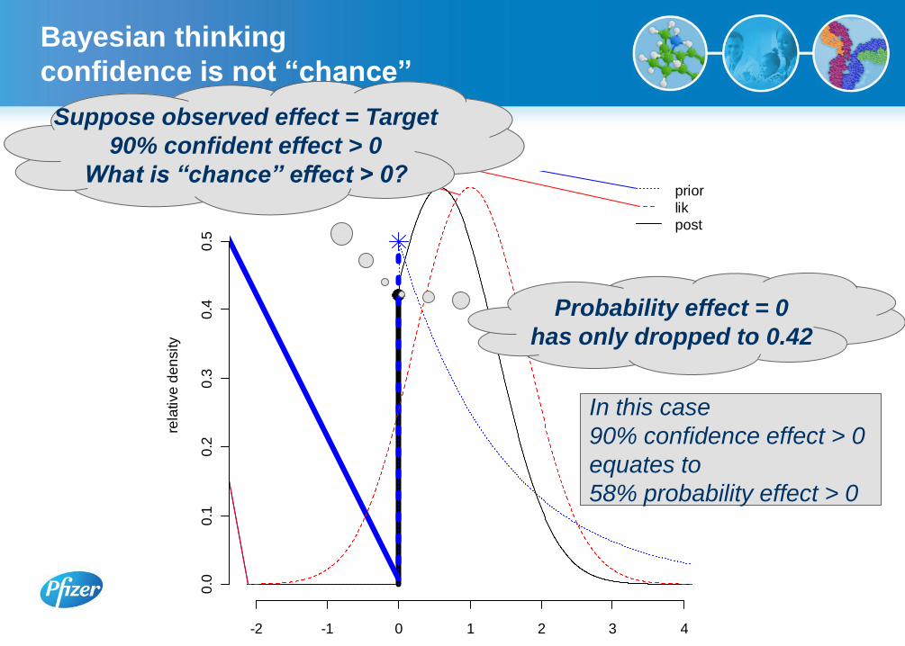
-2 -1 0 1 2 3 4
0.0
0.1
0.2
0.3
0.4
0.5
prior
lik
post
Suppose observed effect = Target
90% confident effect > 0
What is “chance” effect > 0?
Probability effect = 0
has only dropped to 0.42
In this case
90% confidence effect > 0
equates to
58% probability effect > 0
Bayesian thinking
confidence is not “chance”

“Extraordinary claims require extraordinary evidence”
Bayesian thinking
confidence is not “chance”

Calibration of p Values for Testing Precise Null Hypotheses
T.Sellke, M.J.Bayarri, and J.O.Berger
The American Statistician, February 2001, Vol. 55, No. 1
They showed that
“confidence” was
optimistic no matter
what shape the
prior distribution of
non-zero effects.
Bayesian thinking
confidence is not “chance”
Conclusions
• Sample size
High variability of primary endpoint low power or large sample size
Published data can be used for an informative prior, reducing sample size
• Utility of interim analysis.
Resource saving if stopping
Accelerate future work if interim analysis suggests compound efficacious
Probability of being able to make stop or accelerate decision
• Bayesian framework
Novel approach Education (team, management, ethics/regulators)
At design stage
Incorporation of priors
Unconditional probabilities of success
Flexibility in selecting decision criteria
Leads to more thorough thinking
At end of study
Flexible decision criteria and probability statements

27