AE development at Western University: Microseismic monitoring of the olivine → spinel transition in fayalite under non-hydrostatic stress

Acoustic Emission WorkshopJan. 29-31, 2016

GSECARS

The advanced Photon Source

Tim Officer, PhD candidate

University of Western Ontario

Supervisor: Dr. Richard A. Secco

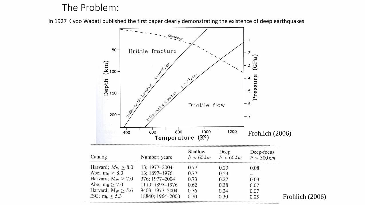
The Problem:In 1927 Kiyoo Wadati published the first paper clearly demonstrating the existence of deep earthquakes

Frohlich (2006)

Frohlich (2006)

Dehydration Embrittlement(e.g. serpentinite, antigorite)

a→g transition in Olivine

Shallow Earthquakes

Green, 1994

Green, 2005

Natural Olivine(Mg1.8, Fe0.2)SiO4

FayaliteFe2SiO4

Olivine

Spinel

Modified Spinel

Ono et al., 2013

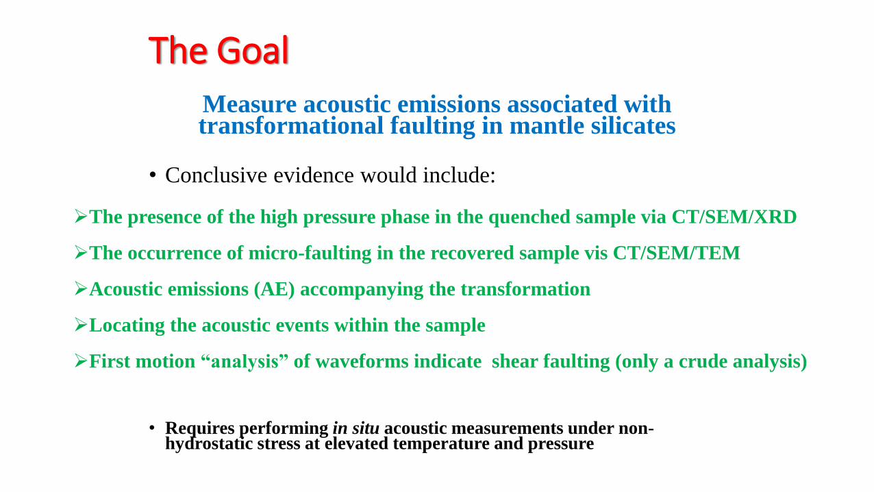
The GoalMeasure acoustic emissions associated with transformational faulting in mantle silicates

• Conclusive evidence would include:

• Requires performing in situ acoustic measurements under non-hydrostatic stress at elevated temperature and pressure

The presence of the high pressure phase in the quenched sample via CT/SEM/XRD

The occurrence of micro-faulting in the recovered sample vis CT/SEM/TEM

Acoustic emissions (AE) accompanying the transformation

Locating the acoustic events within the sample

First motion “analysis” of waveforms indicate shear faulting (only a crude analysis)

00-046-1045 (*) - Quartz, syn - SiO2 - Hexagonal - P3221 (154)

00-034-0178 (*) - Fayalite, syn - Fe2+2SiO4 - Orthorhombic - Pmnb (62)

Y + 2.0 mm - IDEN=TIMOFAY - File: TIMOFAY.raw - Type: 2Th/Th locked - Start: 10.000 ° - End: 90.000 ° - Step: 0.050 ° - Step time:

Lin

(C

ou

nts

)

0

1000

2000

3000

4000

5000

6000

7000

8000

9000

2-Theta - Scale

15 20 30 40 50 60 70 80 90

XRD Pattern for sample of

synthesized Fayalite

from Hematite (Fe2O3) and Quartz (SiO2)

FayaliteQuartz

The fayalite was synthesized in a gas mixing furnace with the help of Dr. Tony Withers at the University of Minnesota

Starting powder

Fayalite Sintering Experimental Assembly

1. Fayalite powder

2. Ag sample container

3. BN

4. Graphite furnace

5. ZrO2

6. Pyrophyllite

1

2

3

4

5

6

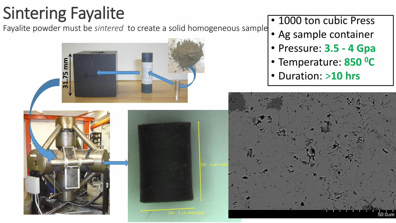
Sintering FayaliteFayalite powder must be sintered to create a solid homogeneous sample

• 1000 ton cubic Press• Ag sample container• Pressure: 3.5 - 4 Gpa• Temperature: 850 0C• Duration: >10 hrs

31

.75

mm

High Pressure, High Temperature,In Situ Acoustic Emission Experiments on Sintered Fayalite

Experimental Setup

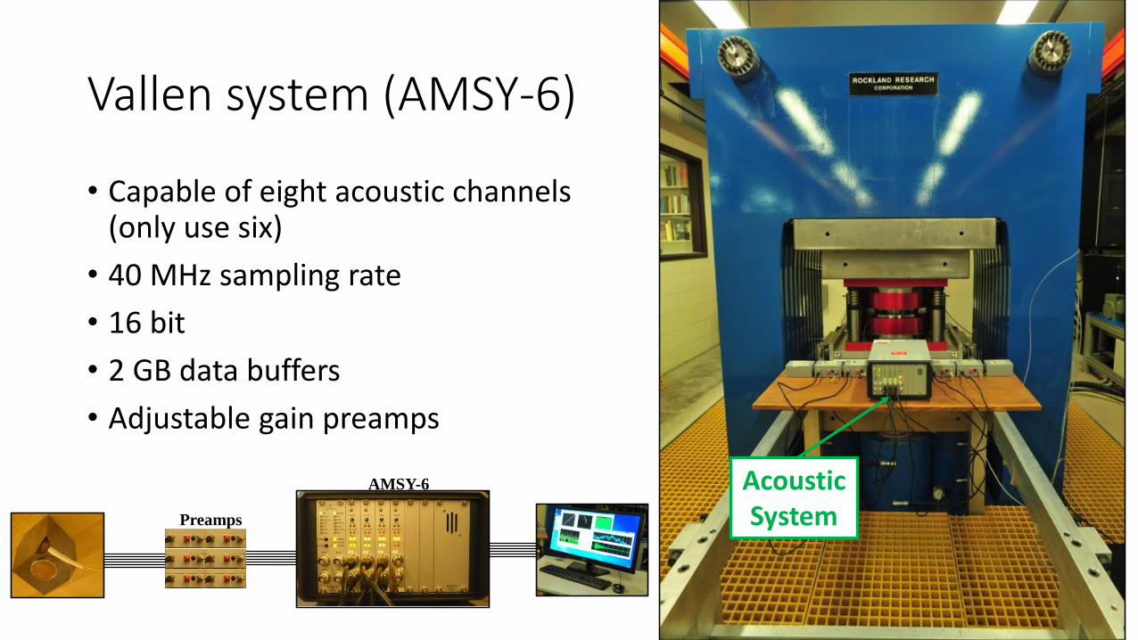
Vallen system (AMSY-6)

• Capable of eight acoustic channels (only use six)

• 40 MHz sampling rate

• 16 bit

• 2 GB data buffers

• Adjustable gain preamps

AMSY-6

Preamps

Acoustic System

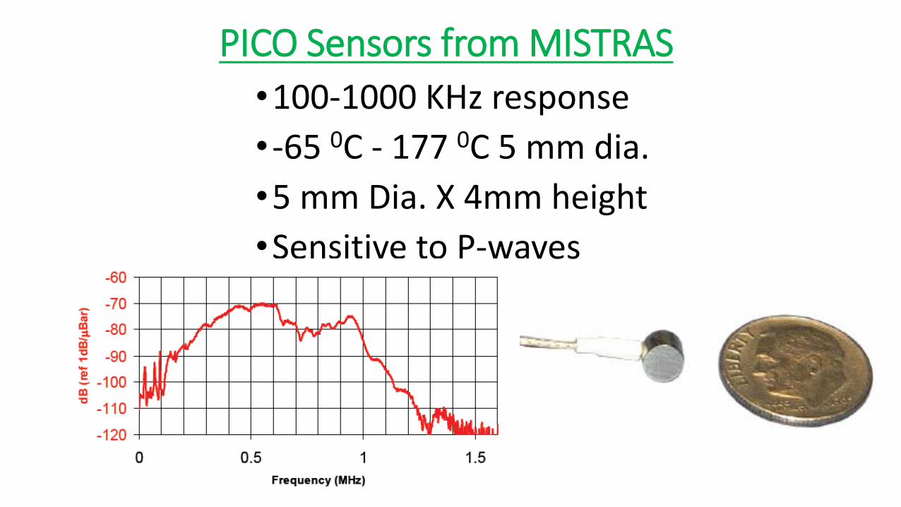
PICO Sensors from MISTRAS

•100-1000 KHz response

• -65 0C - 177 0C 5 mm dia.

•5 mm Dia. X 4mm height

•Sensitive to P-waves

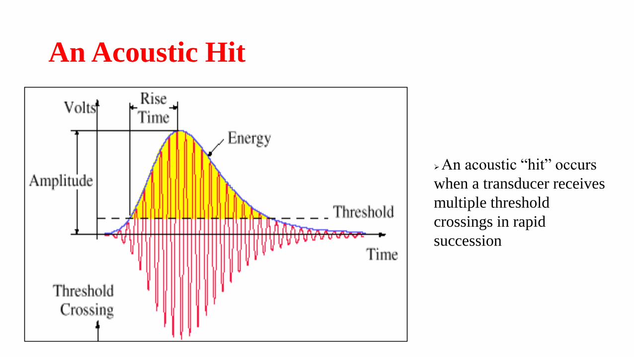
An Acoustic Hit

An acoustic “hit” occurs

when a transducer receives

multiple threshold

crossings in rapid

succession

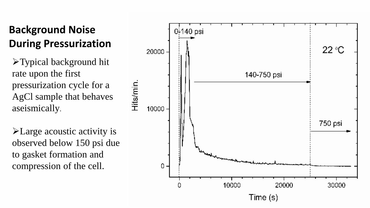
Typical background hit

rate upon the first

pressurization cycle for a

AgCl sample that behaves

aseismically.

Large acoustic activity is

observed below 150 psi due

to gasket formation and

compression of the cell.

Background Noise During Pressurization

Normal Signal

Noise Signal

The pump for the press induces electrical noise in the transducers

Inserted Diamonite between the cubes and 3 of 6 Transducers

Pressurization to 1.5 - 5 GPa• Spurious signals were removed as a

result of the DiamoniteTM discs

• The RMS noise was also substantially reduced

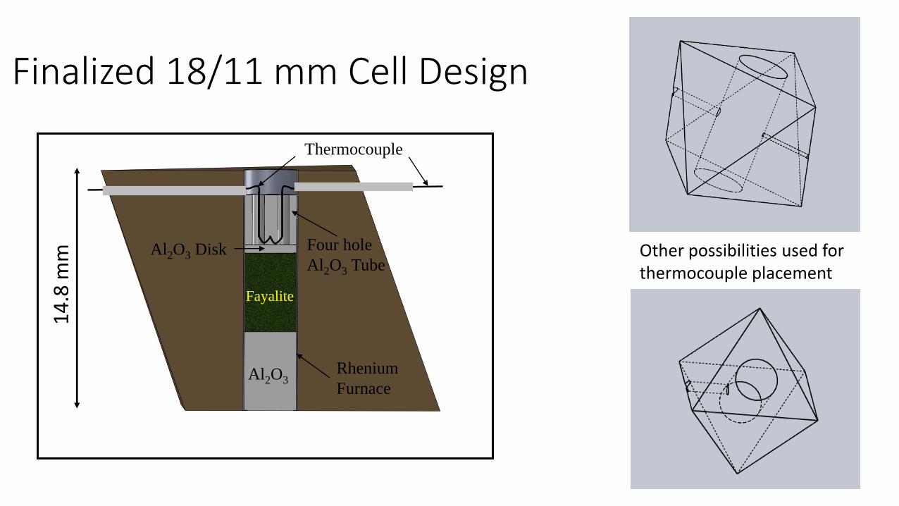
Finalized 18/11 mm Cell Design

Thermocouple

14

.8 m

m

Fayalite

Al2O3

Al2O3 Disk

Rhenium

Furnace

Four hole

Al2O3 Tube

Thermocouple

Other possibilities used for thermocouple placement

Temperature Calibration Experiment: Calibrating temperature at the thermocouple position to the center of the sampleObjective 2: Test Pressure Transducer using the Vallen system

4 hole Al2O3

ceramic tube

4 hole Al2O3 plug

4 hole Al2O3

ceramic tube

Furnace

14

.8 m

m

Thermocouple

Thermocouple

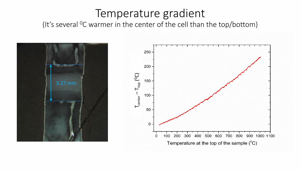
Temperature gradient(It’s several 0C warmer in the center of the cell than the top/bottom)

3.27 mm

T cen

ter–

T top

(0C

)

Hot Pressed Fayalite Experiments - standardized procedure (but with varying P,T and deformation rate conditions)

• Pressurized slowly to desired confining pressure

• Let sit

• Resume slow pressurization and began heating

• Heated to desired temperature

• Resume pressurization to initiate deformation in the spinel stability field

• Depressurize slowly to avoid fracture upon decompression

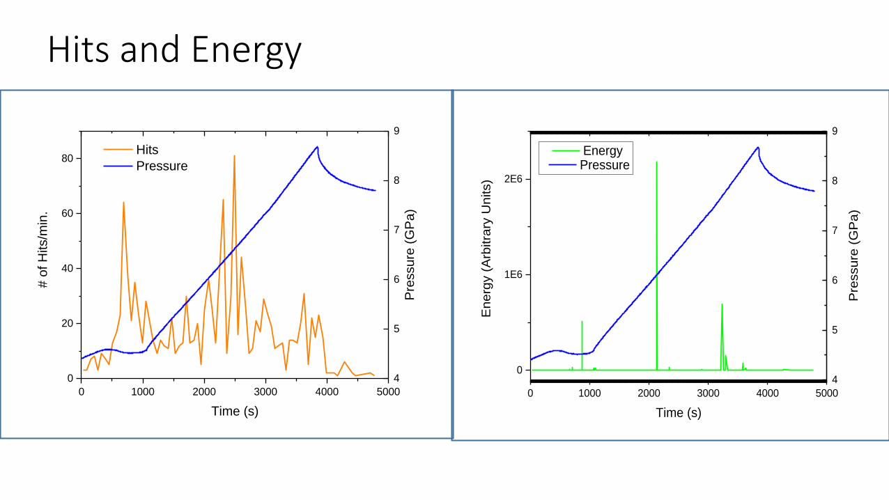
Hits and Energy

0 1000 2000 3000 4000 5000

0

20

40

60

80

# o

f H

its/m

in.

Time (s)

4

5

6

7

8

9

Hits

Pressure

Pre

ssure

(G

Pa)

0 1000 2000 3000 4000 5000

0

1E6

2E6

Energ

y (

Arb

itra

ry U

nits)

Time (s)

Energy

Pre

ssure

(G

Pa)

4

5

6

7

8

9

Pressure

Events >= 4 hits; <50 ms

0 2000 4000

0

1

2

3

# o

f E

ve

nts

(/3

2 s

)

Time (s)

Events

4

5

6

7

8

9

Pressure

Pre

ssure

(G

Pa)

Event Location

Velocity and Transducer Position estimation

Anvils

PulsingTransducer

ReceivingTransducer

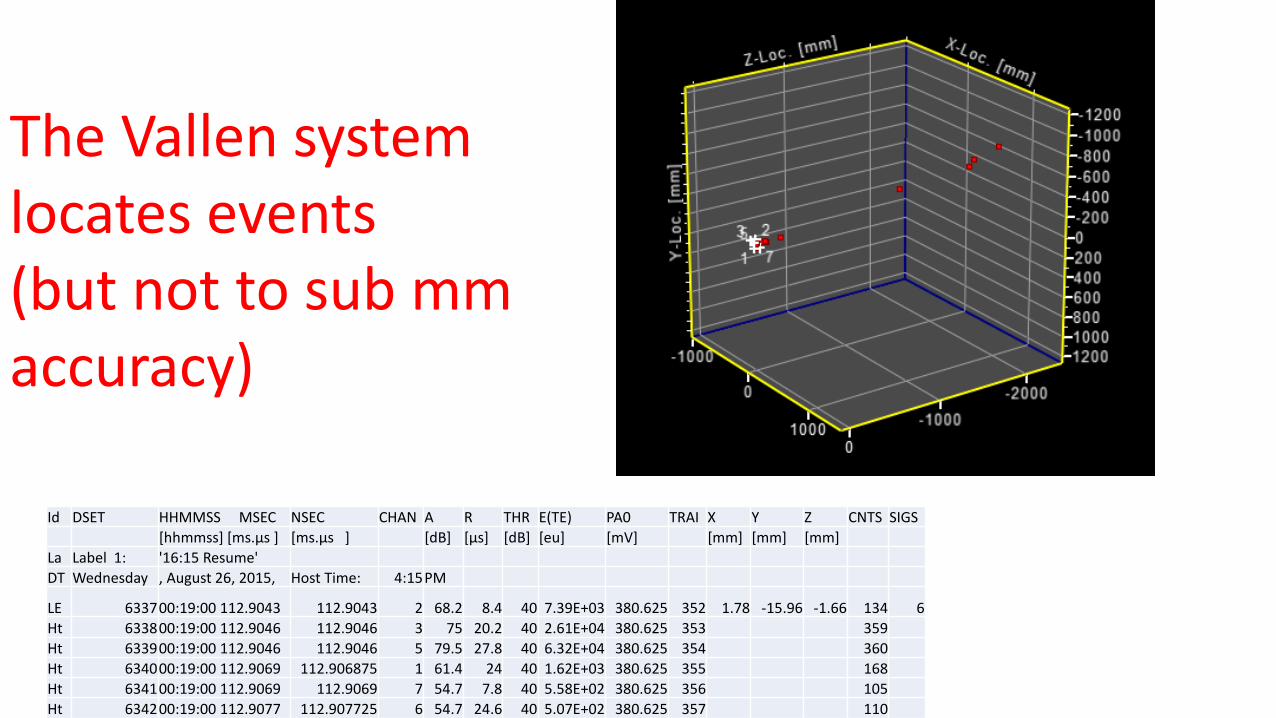
The Vallen system locates events(but not to sub mm accuracy)

Id DSET HHMMSS MSEC NSEC CHAN A R THR E(TE) PA0 TRAI X Y Z CNTS SIGS

[hhmmss] [ms.µs ] [ms.µs ] [dB] [µs] [dB] [eu] [mV] [mm] [mm] [mm]

La Label 1: '16:15 Resume'

DT Wednesday , August 26, 2015, Host Time: 4:15PM

LE 633700:19:00 112.9043 112.9043 2 68.2 8.4 40 7.39E+03 380.625 352 1.78 -15.96 -1.66 134 6

Ht 633800:19:00 112.9046 112.9046 3 75 20.2 40 2.61E+04 380.625 353 359

Ht 633900:19:00 112.9046 112.9046 5 79.5 27.8 40 6.32E+04 380.625 354 360

Ht 634000:19:00 112.9069 112.906875 1 61.4 24 40 1.62E+03 380.625 355 168

Ht 634100:19:00 112.9069 112.9069 7 54.7 7.8 40 5.58E+02 380.625 356 105

Ht 634200:19:00 112.9077 112.907725 6 54.7 24.6 40 5.07E+02 380.625 357 110

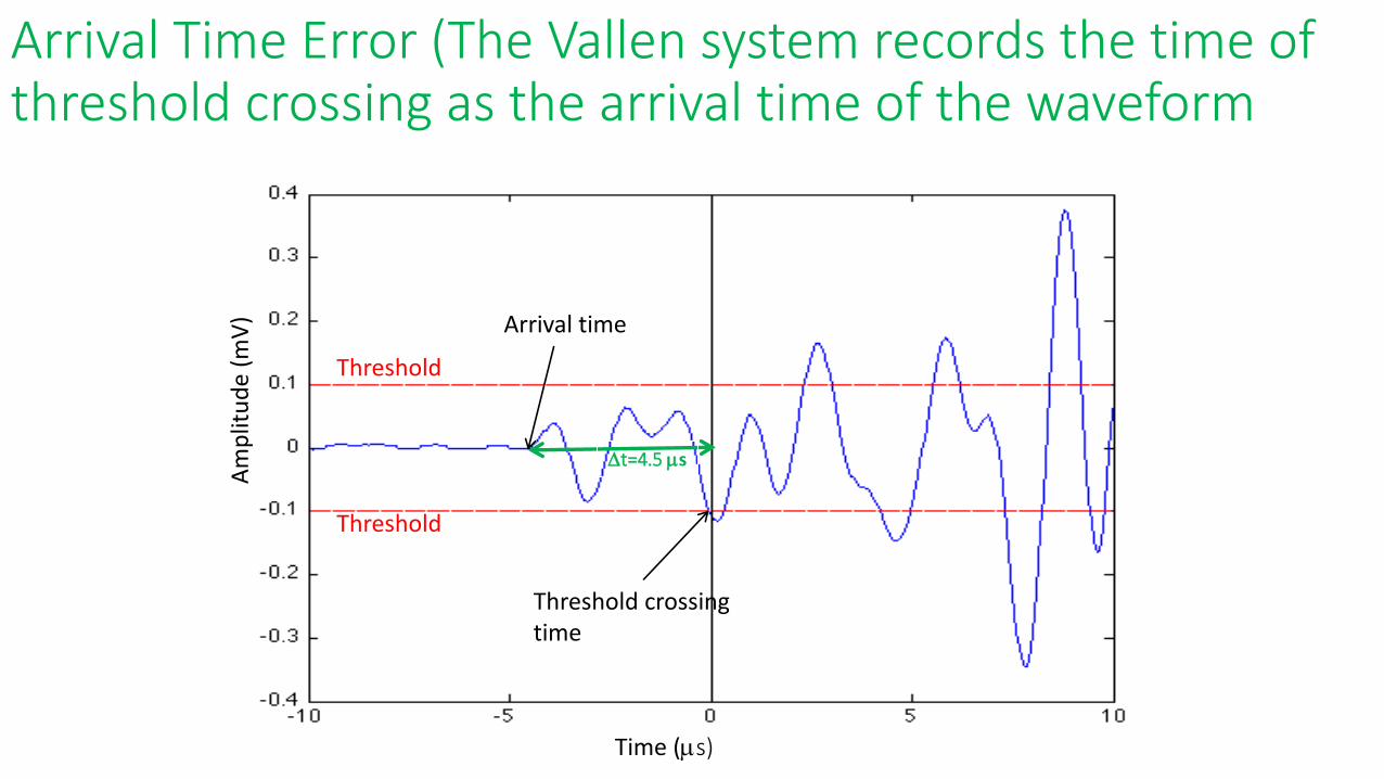
Arrival Time Error (The Vallen system records the time of threshold crossing as the arrival time of the waveform

Am

plit

ud

e (

mV

)

Time (ms)

Dt=4.5 ms

Threshold

Threshold

Threshold crossing time

Arrival time

Akaike Information Criterion (AIC)Automatic Arrival Time Picker

• Separates the signal into two separate signals (background noise and waveform)

• Compares the natural log of the variances of the two signals from 1:n and from n+1:n_samp for each point in the data

• The arrival time is point corresponding to the minimum of the AIC function (i.e when difference in variances is largest)

• To use this algorithm you need to select the right size window since it is an auto-recursive process

))):1(ln(var()1()))1(ln(var()( nsampkyknsampkykkAIC

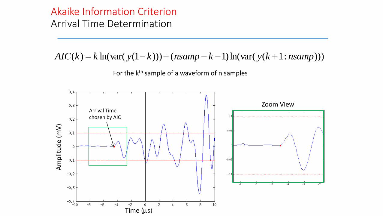
Akaike Information Criterion Arrival Time Determination

))):1(ln(var()1()))1(ln(var()( nsampkyknsampkykkAIC A

mp

litu

de

(m

V)

Time (ms)

Zoom View

For the kth sample of a waveform of n samples

Arrival Time chosen by AIC

0

5

10

15

20

25

30

35

40

45

-30

-29

-28

-27

-26

-25

-24

-23

-22

-21

-20

-19

-18

-17

-16

-15

-14

-13

-12

-11

-10 -9 -8 -7 -6 -5 -4 -3 -2 -1 0 1 2 3 4 5 6 7 8 9

10

11

12

13

14

15

16

17

18

19

20

21

22

23

24

25

26

27

28

29

30

Difference in visual and AIC picks for 135 picks

Nu

mb

er

of

Pic

ks

Difference in Manual and AIC picks (# of points)

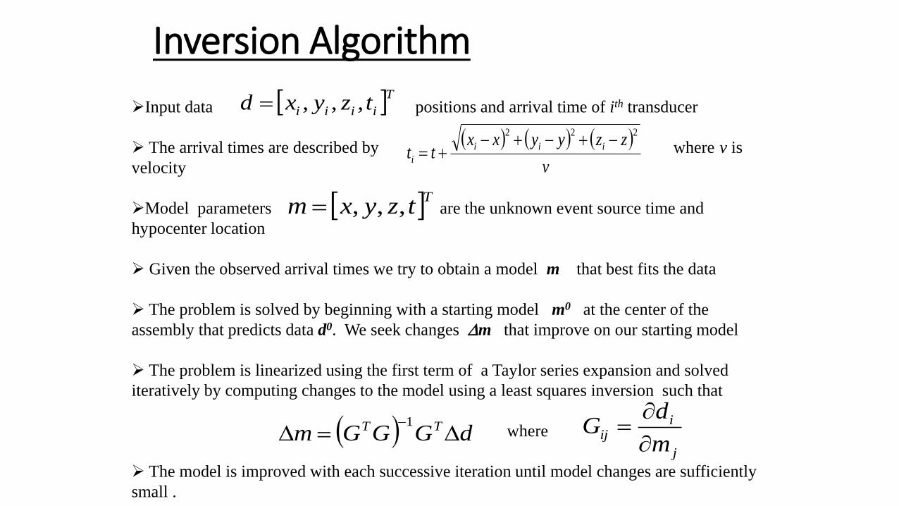
Inversion Algorithm

Input data positions and arrival time of ith transducer

The arrival times are described by where v is

velocity

Model parameters are the unknown event source time and

hypocenter location

Given the observed arrival times we try to obtain a model m that best fits the data

The problem is solved by beginning with a starting model m0 at the center of the

assembly that predicts data d0. We seek changes Dm that improve on our starting model

The problem is linearized using the first term of a Taylor series expansion and solved

iteratively by computing changes to the model using a least squares inversion such that

where

The model is improved with each successive iteration until model changes are sufficiently

small .

Ttzyxm ,,,

Tiiii tzyxd ,,,

v

zzyyxxtt

iii

i

222

dGGGm TT DD1

j

iij

m

dG

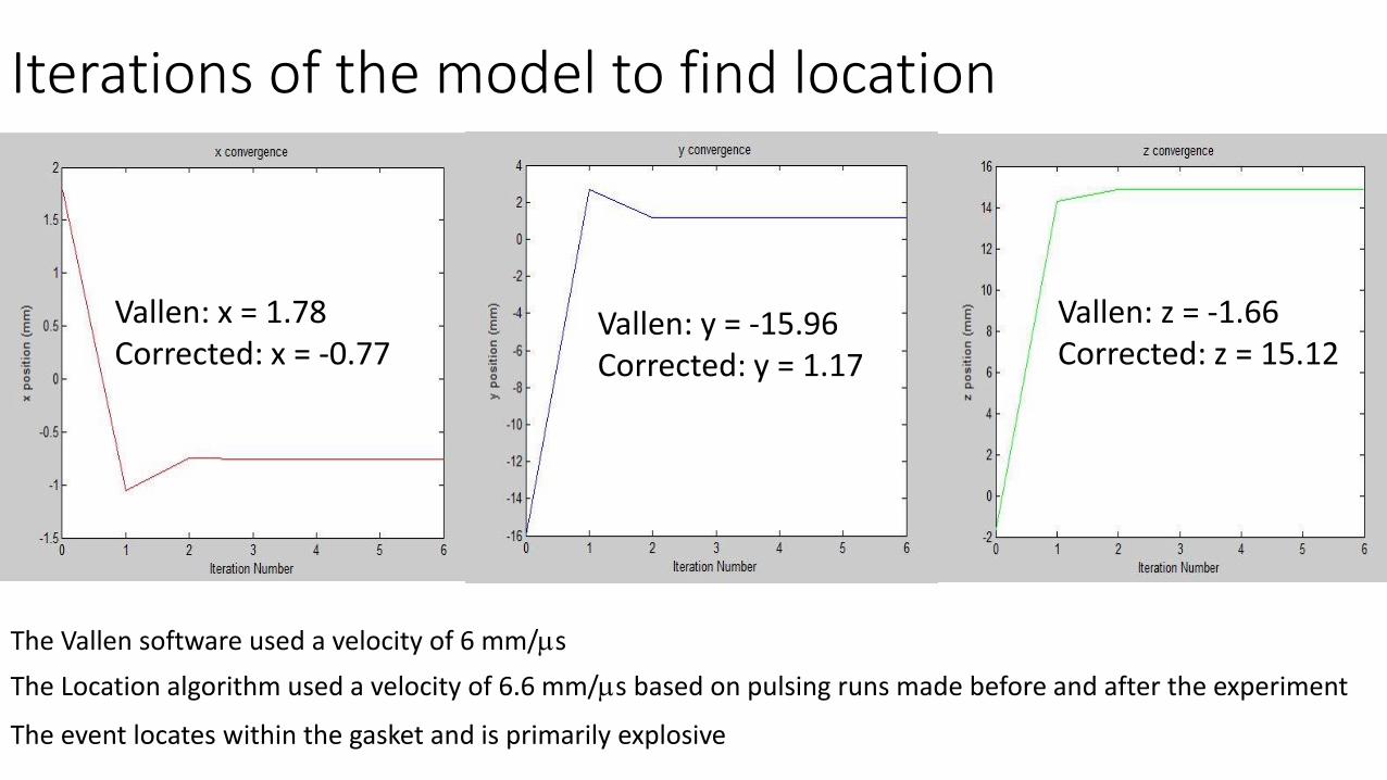
Iterations of the model to find location

Vallen: x = 1.78Corrected: x = -0.77

Vallen: y = -15.96Corrected: y = 1.17

Vallen: z = -1.66Corrected: z = 15.12

The Location algorithm used a velocity of 6.6 mm/ms based on pulsing runs made before and after the experiment

The Vallen software used a velocity of 6 mm/ms

The event locates within the gasket and is primarily explosive

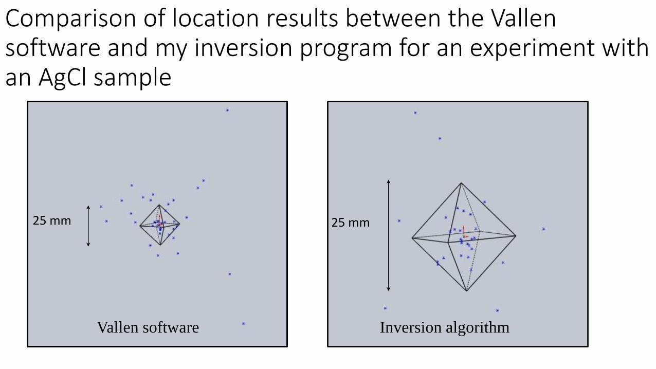
Comparison of location results between the Vallensoftware and my inversion program for an experiment with an AgCl sample

25 mm

Vallen software

25 mm

Inversion algorithm

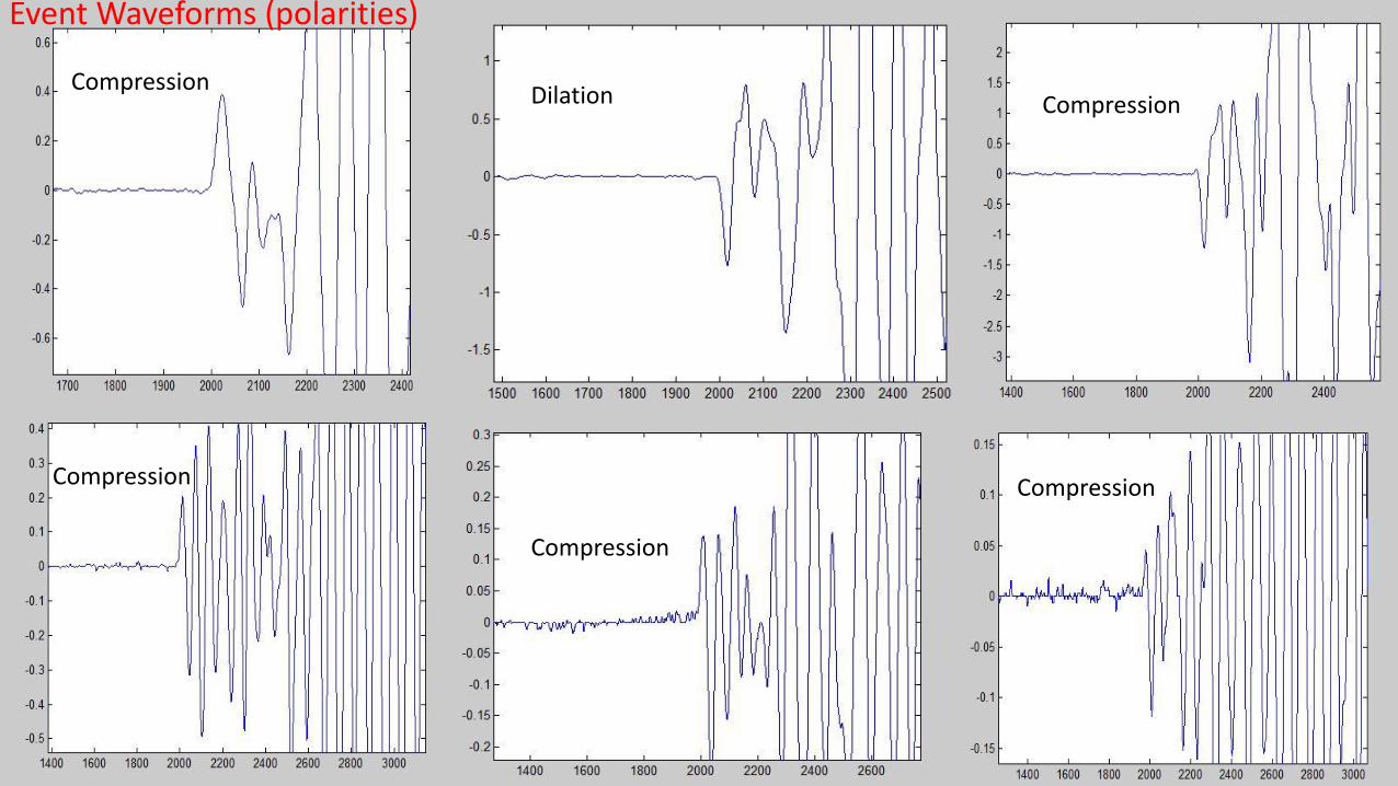
Event Waveforms (polarities)

Compression

Compression

Compression

CompressionDilation

Compression

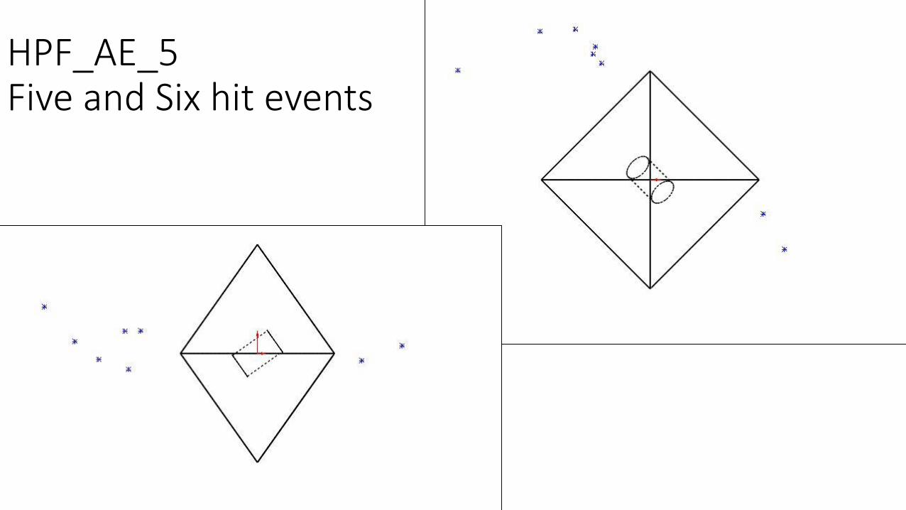
HPF_AE_5Five and Six hit events

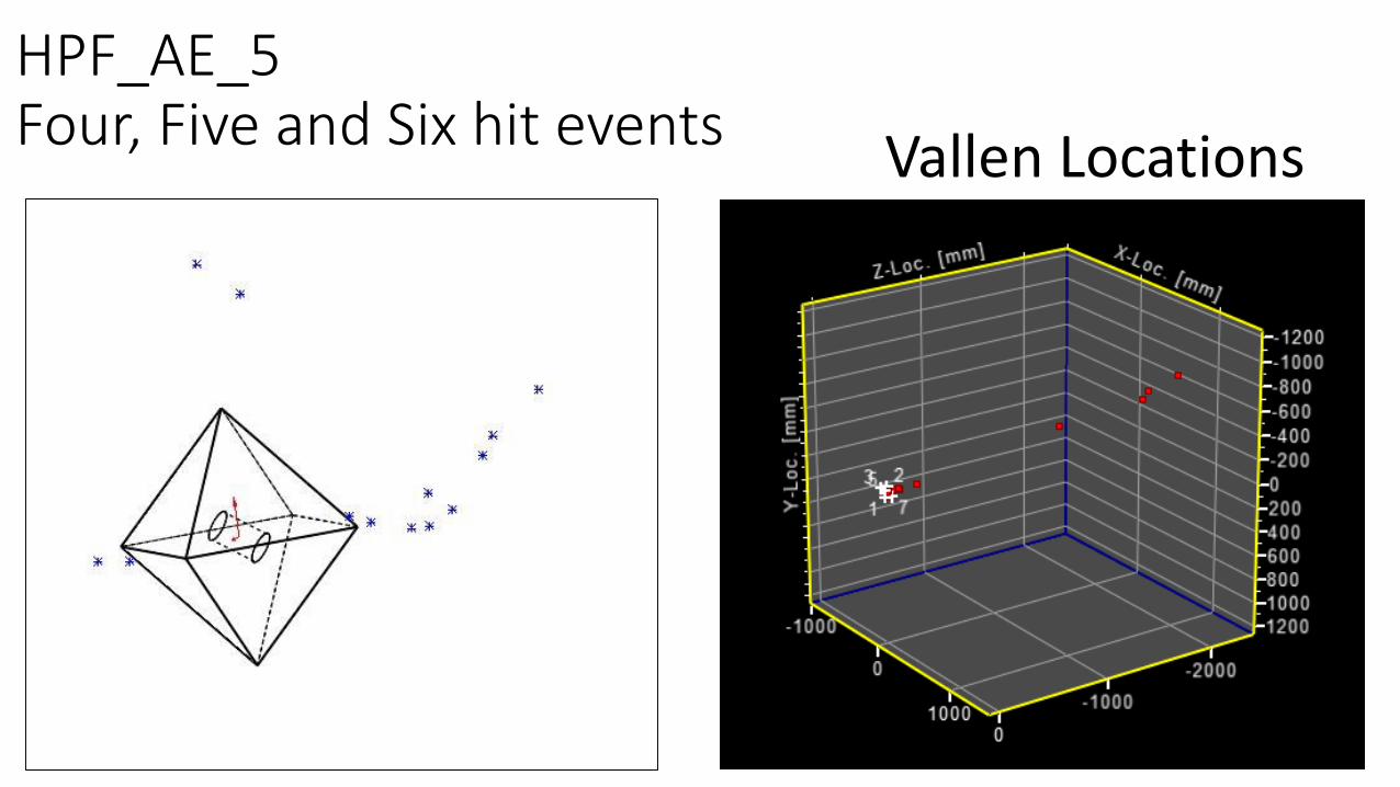
HPF_AE_5Four, Five and Six hit events

Vallen Locations

HPF_AE_5: Strain

Strain ~= 41%Strain Rate ~= 1.36 x 10-3

Fe2SiO4

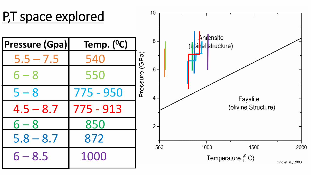
Ono et al., 2003

P,T space explored

6 – 8 850

5.5 – 7.5 540

5.8 – 8.7 872

4.5 – 8.7 775 - 913

5 – 8 775 - 950

6 – 8.5 1000

6 – 8 550

Pressure (Gpa) Temp. (0C)

Future Work

• All of the processes involved in designing and constructing my experiments has been accomplished and the system is in full working order.

• Run ~5-10 more experiments on hot pressed fayalite samples with in situ acoustic monitoring under varying conditions of pressure, temperature and strain rate to induce HPHT faulting

• CT scan recovered samples to look for microstructures associated with faulting

• Grind and polish the samples to look for traces of microstructures associated with faulting.

Hg Experiment: Measuring the transition from Liquid to Solid Hg using discontinuity in travel time

Anvils

PulsingTransducer

ReceivingTransducer

Cell Design and Geometry

“Double Capsule”

Sample Container

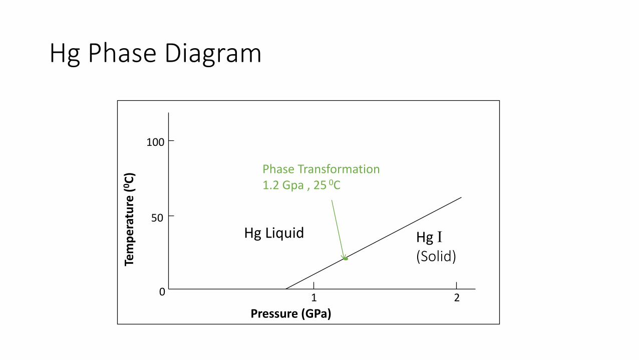
Hg Phase Diagram

0

Tem

pe

ratu

re (

0C

) Phase Transformation1.2 Gpa , 25 0C

Hg Liquid Hg I(Solid)

Pressure (GPa)

50

100

1 2

Measuring Travel Time Along Three Axis

A total of six transducers

provides three sets of

acoustic paths through the

sample: one parallel to the

sample axis and two oblique

at an angle of 70.5 0.

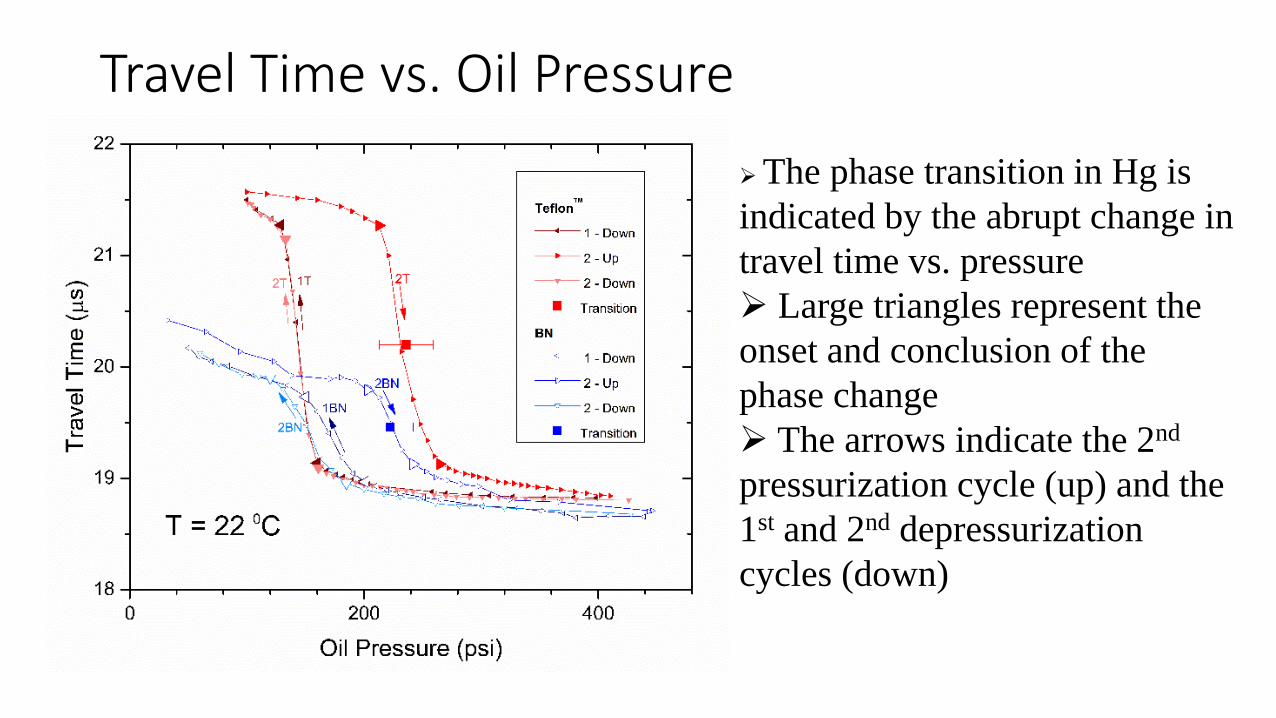
Travel Time vs. Oil Pressure

The phase transition in Hg is

indicated by the abrupt change in

travel time vs. pressure

Large triangles represent the

onset and conclusion of the

phase change

The arrows indicate the 2nd

pressurization cycle (up) and the

1st and 2nd depressurization

cycles (down)

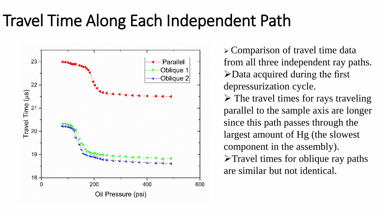
Travel Time Along Each Independent Path

Comparison of travel time data

from all three independent ray paths.

Data acquired during the first

depressurization cycle.

The travel times for rays traveling

parallel to the sample axis are longer

since this path passes through the

largest amount of Hg (the slowest

component in the assembly).

Travel times for oblique ray paths

are similar but not identical.

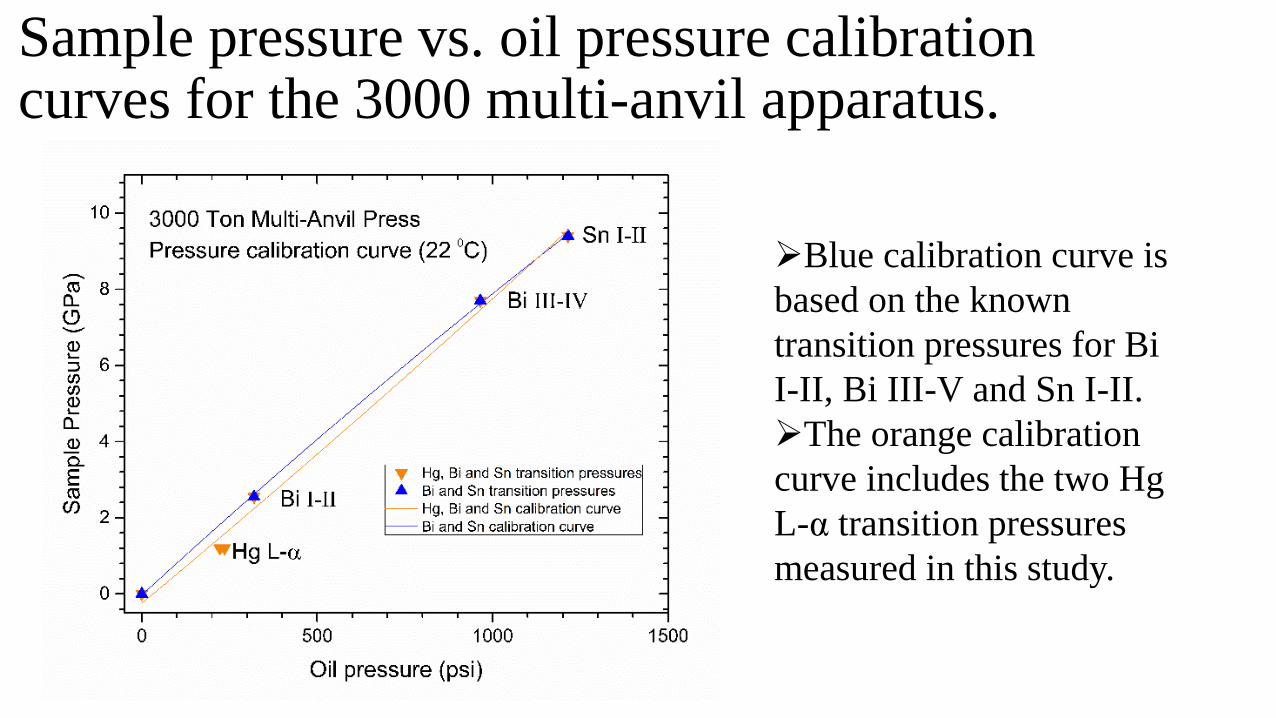
Sample pressure vs. oil pressure calibration curves for the 3000 multi-anvil apparatus.

Blue calibration curve is

based on the known

transition pressures for Bi

I-II, Bi III-V and Sn I-II.

The orange calibration

curve includes the two Hg

L-α transition pressures

measured in this study.

Questions/Advice ?/!References:

Akaogi, et al., 1989. Olivine-modified

spinel-spinel transitions in the Mg2SiO4-

Fe2SiO4: Calorimetric measurements,

thermochemical calculation, and geophysical

application, Journal of Geophysical

Research, 94, 15671

Ono S. et al, 2013. In situ observation of a

phase transition in Fe2SiO4 at high pressure

and high temperature, 40, 811-816

Frohlich, C., 2006. Deep Earthquakes,

Cambridge Univ. Press. Cambridge, England

References (cont.):

Green, H.W., 2005. New light on deep

earthquakes, Scientific American, 97-105

Green, H.W., 1994. Solving the paradox of deep

earthquakes, Scientific American, 64-71

Officer T., and Secco, R.A., 2015, Detection of a

P-induced liquid ⇌ solid-phase transformation

using multiple acoustic transducers in a multi-

anvil apparatus, High Pressure Research, 35, 289

- 299