ae4 final report
TRANSCRIPT

London Office Buildings Tender Report 09.05.2016
10 Storey Office, City Road, London.
1
Executive summary
.This report describes and evaluates the relative merits of several physical changes to the proposed
office block on City Road, London. The heating, ventilation and air conditioning systems are sized
in order to provide adequate fresh air quality and a comfortable working environment for the
workspace. In addition to this, improvements to the materials in the external façade, solar
shielding and changes to the internal design temperatures are simulated with a breakdown of the
reduction in annual energy demand, and the related cost and emissions savings.
The heating demand remained constant throughout, except during internal temperature changes,
which achieved a 9.2% reduction in annual heating demand. By introducing an external façade
with a higher thermal mass, a reduction of 5.2% annual Cooling demand and 3.8% annual fan
power demand were achieved. Introducing the temperature changes achieved a further 1.1%
reduction for cooling and 1.8% for Fan power. By the use of complete solar shielding instead of
temperature changes, a 45.2% reduction in cooling and 52.7% reduction in Fan energy demands
were achieved. Solar shielding was by far the most effective change.
With all physical changes, a total saving of £43925 and 225,183kg of c𝑂2 emission per year can be
achieved due to the reduction in energy demand from 163.87kWh/𝑚2 to 113.61kWh/𝑚2.
The current vertical transport system is insufficient to meet modern building standards. The lift
shaft should be enlarged to occupy a 1.1 by 1.4m, 1000kg lift car.
Similarly, 2 fire exit doors per floor must be introduced to reduce maximum travel distance.
(250)
2

Nomenclature
Qf Fabric Heat Loss (W)
U Thermal transmittance of the material (W/m2.K)
Ti Internal air temperature (oC)
To External air temperature (oC)
A Total Surface area (m2)
ρ Density of Air (Kg/m3)
Qv Ventilation Heat Loss (W)
qv Volumetric flow rate through opening (m3/s)
Cp Specification heat capacity of air (J/Kg.K)
V Volume of room (m2)
Qg Sensible heat gain through glazing (W/m2.K)
Ag Total glazed area (m2)
Ug U value of glazing (W/m2.K)
Qsg Solar gain through glazing (W)
qsg Tabulated Cooling Load (W/m2)
G G value correction factor
CF Correction factor for building response
QΘ+Φ Heat flow into room Φ hours after solar incidence
Te Sol air temperature at time Θ
ƒ Decrement factor
gs Supply moisture content
gr Room moisture content
LH Latent heat gains (W)
L Latent heat of vaporisation capacity
M Mass Flow Rate (m2/s) 3
Nomenclature
HT Total peak casual heat gains (W)
ΔT Difference in air temperature (oC)
Csa Cross sectional area (m2)
Re Reynolds number
v velocity (m/s)
d Diameter of Duct
μ Viscosity (N/m2)
k Roughness coefficient
λ Friction factor
ΔP Pressure drop (Pa)
ΔPFriction Pressure drop due to friction (Pa)
l Length (m)
ζ component loss coefficient
A2 Csa after contraction (m2)
A1 Csa before contraction (m2)
Δpcontration Pressure loss due to contraction (m2)
qs Flow rate after component (m3/s)
qc Flow rate before component (m3/s)
Δpcomponent Pressure drop due to component (Pa)
ΔpTotal Total pressure drop (Pa)
Pair Power transferred to the air by the fan (W)
QT Total Flow Rate (m3/s)
Pelec Electric power supplied to the fan (W)
P Number of people served
w Width of stairs (m2)4

Contents
.Section Page Number
Executive Summary 2
Nomenclature 3
Contents 4
1. Introduction 9
2. Building Information
2.1 Geometry and Internal layout 10
2.2 Occupancy 12
2.3 Ventilation 12
2.4 Fabric types and properties 13
2.5 Air permeability and infiltration rate 13
2.6 Casual heat gains 14
2.7 Thermal conductance 14
3. Extreme Conditions – Heating Season
3.1 Environmental conditions 15
3.2 Fabric heat losses by type 15
3.3 Ventilation losses 16
3.4 Heat gains 17
4. Extreme Conditions – Cooling Season
4.1 Sensible transmission through the glazing 19
4.2 Solar gains through windows 19
4.3 Sol-air gains 20
4.4 Sol-air roof gains 20
4.5 Casual heat gains 20
5
Contents
.Section Page Number
4. Extreme conditions – Cooling season
4.6 Ventilation heat gains 21
4.7 Peak cooling load 22
5. Boiler Plant
5.1 Boiler sizing 23
5.2 Running costs and emissions 23
6. Air Conditioning
6.1 Sizing the air conditioning system (ACS) 24
6.2 Psychometric process 24
6.2.1 Simulation 1 24
6.2.2 Simulation 2 27
6.3 Design criterion, ACS type 27
6.4 ACS Mechanism, components and air handling
unit (AHU) components 28
6.4.1 ACS mechanism 28
6.4.2 ACS components 28
6.4.3 AHU components 28
6.5 Control strategy 29
6.6 Gross annual running costs 29
7. Ventilation
7.1 Duct configuration 31
7.2 Summer design criteria 32
7.3 Sanitary and non-sanitary and return air paths 33
7.4 pressure drop and supply index run 356

Contents
.Section Page Number
7. Ventilation
7.5 Pressure loss due to component 37
7.6 Supply diffuser choice 40
7.7 Gross costs, carbon emissions and AHU fans 42
7.7.1 Cost considerations 43
8. Sensitivity Analysis
8.1 Heating 46
8.2 Cooling 46
8.3 Fan energy demand 47
8.4 Total energy demand 47
8.5 Relative merit of each change 48
9. Fire Safety
9.1 Compartmentalization 49
9.2 Horizontal escape 49
9.3 Vertical escape 51
9.4 Protection of ventilation openings 52
9.5 Detection 52
9.6 Hose reels 53
9.7 Sprinklers 55
9.8 Hydrants, risers and landing valves 56
10. Vertical Transport
10.1 Background 59
10.2 Method 59
10.3 Results 417

Contents
.Section Page Number
10. Vertical transport
10.4 Estimating suitability of lift size 62
10.5 Additional information and analysis 63
11. Conclusion 64
12. References 65
13. Appendix 69
14. CV’s 76
8
1. Introduction
As a specialist building consultancy company, we aim to provide our clients with a
detailed analysis of the solutions we can offer. We create practical energy efficient
solutions, whilst achieving comfortable and functional design complying to UK
regulations.
The key aim of this report is to ensure the current building design is fit for purpose
under limiting conditions, whilst creating a comfortable working environment
through the building services design.
By the use of 5 manual simulations, the energy demand, cost and emissions, for
differing physical changes proposed for the building, will be assessed. These physical
changes come in the form of varying the decrement factor, lag time, building colour,
and indoor air temperatures, and the use of solar shading.
The aforementioned building services include boiler sizing, the size of the air
conditioning system and number of air handling units (AHU) as well as the fan
systems within these, the proposed ductwork layouts for supply and extract, and the
required number and size of diffusers. Additionally the fire protection systems have
been designed with any required architectural changes stated. Vertical transport
systems are also proposed such that the occupant demand within the building is met,
with any architectural changes needed also provided.
London Office Buildings specified that the heating system was to be gas powered and
the cooling to be electrically powered. (220)9

2. Building Information
2.1. Geometry and Internal Layout.
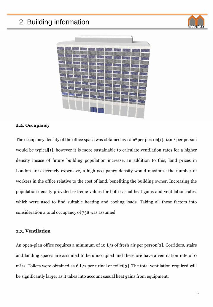
The 10-storey proposed office block faces southeast onto City Road, London. It is
rectangular in shape with 9789m2 internal area. Each upper floor is 3.6m in height and
49.5m x 19.74m in plan. In the center of the space are 2 stairwells, space for ducting and
building services, two stores, separate male and female toilets, and 4 lift shafts all facing
into a central lobby.
Table 2.1, Typical Upper Floor Area
Zone Area (m2)
Office Floor 827.25
Male Toilets 58.50
Female Toilets 54.00
Lifts 7.00
Lobby 40.50
Stairwells 15.14
Duct 3.54
Total 1005.93
10
2. Building Information
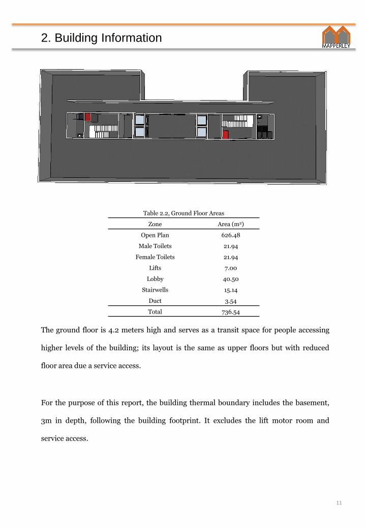
The ground floor is 4.2 meters high and serves as a transit space for people accessing
higher levels of the building; its layout is the same as upper floors but with reduced
floor area due a service access.
Table 2.2, Ground Floor Areas
Zone Area (m2)
Open Plan 626.48
Male Toilets 21.94
Female Toilets 21.94
Lifts 7.00
Lobby 40.50
Stairwells 15.14
Duct 3.54
Total 736.54
For the purpose of this report, the building thermal boundary includes the basement,
3m in depth, following the building footprint. It excludes the lift motor room and
service access.
11
2. Building information
2.2. Occupancy
The occupancy density of the office space was obtained as 10m2 per person[1]. 14m2 per person
would be typical[1], however it is more sustainable to calculate ventilation rates for a higher
density incase of future building population increase. In addition to this, land prices in
London are extremely expensive, a high occupancy density would maximize the number of
workers in the office relative to the cost of land, benefiting the building owner. Increasing the
population density provided extreme values for both casual heat gains and ventilation rates,
which were used to find suitable heating and cooling loads. Taking all these factors into
consideration a total occupancy of 738 was assumed.
2.3. Ventilation
An open-plan office requires a minimum of 10 L/s of fresh air per person[2]. Corridors, stairs
and landing spaces are assumed to be unoccupied and therefore have a ventilation rate of 0
m3/s. Toilets were obtained as 6 L/s per urinal or toilet[3]. The total ventilation required will
be significantly larger as it takes into account casual heat gains from equipment.
12
2. Building information
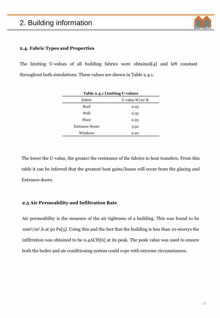
Table 2.4.1 Limiting U-values
Fabric U-value W/m2.K
Roof 0.25
Wall 0.35
Floor 0.25
Entrance Doors 3.50
Windows 2.20
The lower the U-value, the greater the resistance of the fabrics to heat transfers. From this
table it can be inferred that the greatest heat gains/losses will occur from the glazing and
Entrance doors.
2.5 Air Permeability and Infiltration Rate
Air permeability is the measure of the air tightness of a building. This was found to be
10m3/m2.h at 50 Pa[5]. Using this and the fact that the building is less than 10-storeys the
infiltration was obtained to be 0.4ACH[6] at its peak. The peak value was used to ensure
both the boiler and air conditioning system could cope with extreme circumstances.
2.4. Fabric Types and Properties
The limiting U-values of all building fabrics were obtained[4] and left constant
throughout both simulations. These values are shown in Table 2.4.1.
13
2. Building information
2.7 Thermal Conductance
The product of the U-value and the area of the specific building fabric give the thermal
conductance. The sum of the entire thermal conductance’s can then be found. In the case
of this building it equaled 2.784 kW.m2 for both simulations.
(482)
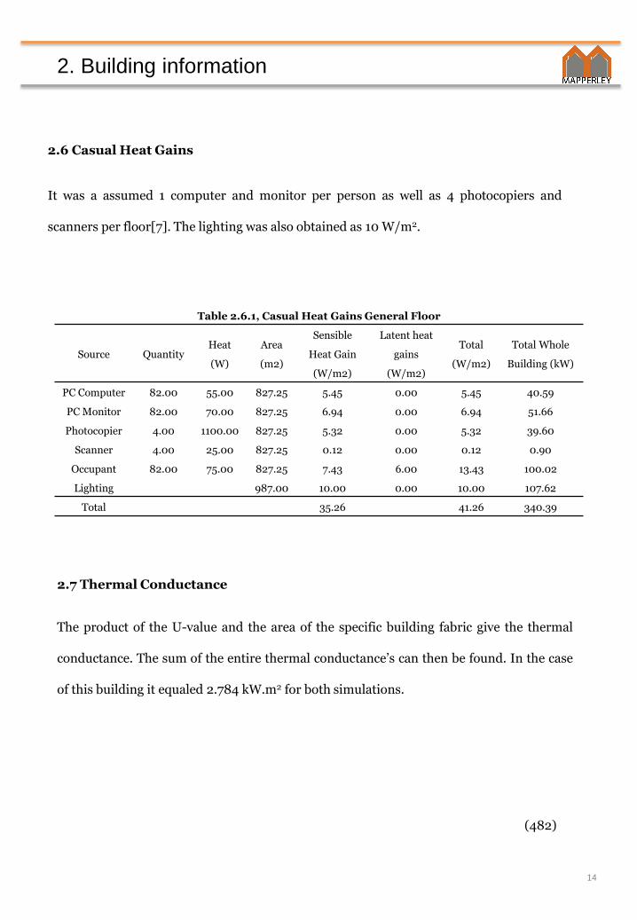
Table 2.6.1, Casual Heat Gains General Floor
Source QuantityHeat
(W)
Area
(m2)
Sensible
Heat Gain
(W/m2)
Latent heat
gains
(W/m2)
Total
(W/m2)
Total Whole
Building (kW)
PC Computer 82.00 55.00 827.25 5.45 0.00 5.45 40.59
PC Monitor 82.00 70.00 827.25 6.94 0.00 6.94 51.66
Photocopier 4.00 1100.00 827.25 5.32 0.00 5.32 39.60
Scanner 4.00 25.00 827.25 0.12 0.00 0.12 0.90
Occupant 82.00 75.00 827.25 7.43 6.00 13.43 100.02
Lighting 987.00 10.00 0.00 10.00 107.62
Total 35.26 41.26 340.39
2.6 Casual Heat Gains
It was a assumed 1 computer and monitor per person as well as 4 photocopiers and
scanners per floor[7]. The lighting was also obtained as 10 W/m2.
14

2. Building Information
Five sets of conditions were applied to the building. These conditions are outlined in
tables 8.1 to 8.4. (18)
Table 8.2, Simulaition 2a
Condition Variable
Condition
Exterior colour Light
Solar Sheilding Total
Decrement Factor 0.2
Lag Time (hrs) 8
Summer Ti C 24
Winter Ti C 19
Table 8.1, Simulaition 1
Condition Variable
Condition
Exterior colour Dark
Solar Sheilding No
Decrement Factor 0.9
Lag Time (hrs) 1
Summer Ti C 22
Winter Ti C 21
Table 8.3, Simulaition 2b
Condition Variable Condition
Exterior colour Light
Solar Sheilding No
Decrement Factor 0.2
Lag Time (hrs) 8
Summer Ti C 24
Winter Ti C 19
Table 8.4, Simulaition 2c
Condition Variable
Condition
Exterior colour Light
Solar Sheilding Total
Decrement Factor 0.2
Lag Time (hrs) 8
Summer Ti C 22
Winter Ti C 21
Table 8.5, Simulaition 2d
Condition Variable Condition
Exterior colour Light
Solar Sheilding No
Decrement Factor 0.2
Lag Time (hrs) 8
Summer Ti C 22
Winter Ti C 21
15

3. Extreme Conditions – Heating Season
3.1 Environmental Conditions
In order to size the boiler for the worst conditions, a temperature of -3°C was used for the
design outdoor temperature, as this temperature is either equalled or exceeded for 99.6% of
the total hours in a year in London [8]. For Simulation 1 a design indoor temperature of 21°C
[9] was the most appropriate in order to neglect heat transfer between rooms, giving a
temperature difference for calculation of 24°C. For Simulation 2a and 2b we reduced this
temperature by 2°C in order to assess the effect of reduced temperature difference on fabric
heat loss.
3.2 Fabric heat losses by type
The steady state conduction fabric losses varied according to the thermal transmittance of
the material on the buildings thermal boundary. The total heat loss for each material was
calculated as in Equation 3.2.1.
Equation 3.2.1, Fabric Heat Loss
𝑄𝐹 = 𝑈𝐴(𝑇𝑖 − 𝑇𝑜)
Where 𝑄𝐹 is the fabric heat loss (W), U is the thermal transmittance of the material (𝑊/𝑚2𝐾), A is the total surface area of each material (𝑚2), 𝑇𝑖 is the index temperature (°C) and 𝑇𝑜 is the external temperature (°C).
Example Calculation 3.2.1, Fabric Heat Loss, Windows, General floor:
𝑄𝐹 = 2.2 × 158.98 24 = 8.394𝑘𝑊
A calculation of the total fabric heat loss per material, per floor, was necessary due to varying surface areas.
16

3. Extreme Conditions – Heating Season
Table’s 3.2.1 and 3.2.2 show the peak fabric heat loss by material type for Simulations 1 and 2n
respectively.
Table 3.2.1 - Fabric loss by type - Simulation 1
Fabric Qf (W)
Windows 77644.61
Walls 28698.74
Roof 5675.25
Floor 545.45
Basement 5837.76
Doors 2225.66
Total 120627.46
Table 3.2.2 - Fabric loss by type - Simulation 2n
Type Qf (W)
Windows 70892.90
Walls 26203.19
Roof 5181.75
Floor 498.02
Basement 5059.39
Doors 2032.13
Total 109867.38
A 10% decrease in fabric heat loss is achieved by decreasing the design indoor
temperature by 2°C. Windows account for almost 65% of the total fabric heat loss and
walls roughly 25%.
3.3 Ventilation losses
Equation 3.3.1, Ventilation heat loss
𝑄𝑉 = 𝑞𝑣𝜌𝑐𝑝 𝑇𝑖 − 𝑇𝑜
For air at ambient temperatures, ρ ≈ 1.20 𝑘𝑔.𝑚−3 and 𝑐𝑝 ≈ 1000 𝐽. 𝑘𝑔−1. 𝐾−1, hence:
𝑄𝑉 = 𝑞𝑣 𝑇𝑖 − 𝑇𝑜 /3
Where, 𝑄𝑉 is the heat transfer by ventilation (W), 𝑞𝑣 is the volumetric flow rate through opening (m3·s–1), 𝑐𝑝 is the specific heat capacity of air (𝐽. 𝑘𝑔−1𝐾−1), ρ is the density of air
(kg·𝑚3), 𝑇𝑖 and 𝑇𝑜 are the indoor and outdoor temperature.
Equation 3.3.2, Volume flow rate
Total volume flow rate, 𝑞𝑣 = Infiltration rate (ACH) + Ventilation rate (ACH) x V
Where, V is the Volume of the room (𝑚2)
17

3. Extreme Conditions – Heating Season
Example Calculation 3.3.2, Ventilation heat loss, Open plan office area, General floor, Simulation 1.
𝑞𝑣 = 0.99 + 0.4 × 2978.1 = 4139.6 𝑚3/𝑠
𝑄𝑉 = 4139.6 23 /3 = 3173.7 𝑊
3.4 Heat gains
It was assumed that the heating season starts on the 1st of October and continues through to
the 1st of May, and that no heating is required during the cooling season (the remainder of the
year). It was also assumed for simplicity that there are no casual heat gains during the
heating period. (235)
18
4. Extreme Conditions – Cooling Season
When sizing the air conditioning system, extreme values were chosen to find the peak-
cooling load. Although for the majority of the time this load will never be reached, the
system needs to have the ability to provide this cooling power if necessary.
To find the peak-cooling load, the heat gains of 6 different variables need to be summed.
Sensible transmission through the glazing
Solar gains through the glazing
Sol-air gains
Roof sol-air gains
Casual heat gains
Ventilation heat gains
These gains are quasi-dynamic (varying with time) as a result of changing outdoor air
temperatures. All examples show results for 11:30 on 21st May, the time found to produce
the peak-cooling load.
19
4. Extreme Conditions – Cooling Season
Equation 4.1.1, Sensible Transmission through the Glazing
𝑄𝑔 = 𝐴𝑔 × 𝑈𝑔 × 𝑡𝑜 − 𝑡𝑖
Where Qg is the sensible gain through the glazing (W), Ag is the total glazed area (m2), Ug is the U-value of theglazing (W/m2.K)[10], ti is the internal air temperature (°C)[11], to is the external air temperature (°C)[12].
Example Calculation 4.1.1, Sensible Transmission through the Glazing, Small Window
𝑄𝑔 = 5.53 × 2.2 × 23 − 22
𝑄𝑔 = 14.45𝑊 per window
4.2. Solar Gains Through Windows
This shows the radiant heat gain through the windows as a result of the sun. It takes into
account building orientation, location, time of day, and glazing configuration (G-value) as
well as the building response factor.
4.1. Sensible Transmission through the Glazing
This is a measure of heat transfer through the glazing as a result of the difference in
internal and external air temperatures.
Equation 4.2.1, Solar Gains through Windows
𝑄𝑠𝑔 = 𝑞𝑠𝑔 × 𝐺 × 𝐶𝐹 × 𝐴
Where Qsg is the solar gains through the glazing (W), qsg is the tabulated cooling load (W/m2)[13], G is the G-Value correction factor for glazing type[13], CF is the correction factor for building response, fast response is 0.83, slow response is 0.72[13], A is window are (m2)
Example Calculation 4.2.1, Solar Gains through Windows, SE Surface
𝑄𝑠𝑔 = 476 × 0.72 × 0.83 × 186.62
𝑄𝑠𝑔 = 174997.41𝑊
This method is repeated for each building surface, which are then summed to find the
total gain.
20
4. Extreme Conditions – Cooling Season
4.3. Sol-air Gains
This is a fictitious outdoor air temperature that allows the heat flow as a result of both
radiant and convective transfer to be calculated.
Equation 4.3.1, Sol-air Gains considering thermal capacity
𝑄𝜃+𝜙 = 𝑈𝐴 𝑡𝑒𝑚 − 𝑡𝑟 + 𝑈𝐴 𝑡𝑒 − 𝑡𝑒𝑚 𝑓
Where Qθ+ϕ is the heat flow into the room ϕ hours after solar incidence (W), U is the U-value for the exterior
wall (W/m2.K)[10], A is the area of the exterior wall (m2), tem is the 24hr mean sol-air temperature (°C)[5], te
sol-air temperature at time (θ) of solar incidence (°C)[14], tr is the room temperature (°C), ƒ is decrement
factor [15].
Example Calculation 4.3.1, Sol-air Gains considering thermal capacity, SE Dark Surfacewith a decrement factor of 0.9 and a lag time of 1hr
𝑄𝜃+𝜙 = 0.35 × 1229.03 27.47 − 22 + 0.35 × 1229.03 55 − 27.47 0.9
𝑄𝜃+𝜙 = 13011.48𝑊
4.4. Sol-air Roof Gains
The sol-air gains for the roof also were found using Equation 4.3.1.
4.5. Casual Heat Gains
Casual heat gains are defined in building specification, section 2.6.
21
4. Extreme Conditions – Cooling Season
4.6. Ventilation Heat Gains
Ventilation heat gains will vary depending on the outdoor air temperature.
Equation 4.6.1, Total Air Change Rate
𝑉𝑒𝑛𝑡𝑖𝑙𝑎𝑡𝑖𝑜𝑛 𝑅𝑎𝑡𝑒 + 𝐼𝑛𝑓𝑖𝑙𝑡𝑟𝑎𝑡𝑖𝑜𝑛 𝑅𝑎𝑡𝑒 = 𝑇𝑜𝑡𝑎𝑙 𝐴𝑖𝑟 𝐶ℎ𝑎𝑛𝑔𝑒 𝑅𝑎𝑡𝑒
Where Ventilation rate (h-1)[16] and Infiltration rate (h-1)[17] can be assumed.
Example Calculation 4.6.1, Total Air Change, Open plan office
0.991 + 0.4 = 1.391
Equation 4.6.2, Ventilation Rate (m3/s)
𝑉𝑜𝑙𝑢𝑚𝑒 × 𝑇𝑜𝑡𝑎𝑙 𝐴𝑖𝑟 𝐶ℎ𝑎𝑛𝑔𝑒 𝑅𝑎𝑡𝑒
3600= 𝑉𝑒𝑛𝑡𝑖𝑙𝑎𝑡𝑖𝑜𝑛 𝑅𝑎𝑡𝑒
Where volume is the volume of the room for which the ventilation rate is being calculated (m3), Total Air Change Rate has been previously calculated (h-1), 3600 is the number of seconds in 1 hour, Ventilation rate is the air changes in the room (m3/s).
Example Calculation 4.6.2, Ventilation Rate (m3/s)
2978.1 × 1.391
3600= 1.151
Equation 4.6.3, Ventilation Thermal Conductance (W/K)
𝑉𝑒𝑛𝑡𝑖𝑙𝑎𝑡𝑖𝑜𝑛 𝑅𝑎𝑡𝑒 × 𝐻𝑒𝑎𝑡 𝐶𝑎𝑝𝑎𝑐𝑖𝑡𝑦 𝑜𝑓 𝑎𝑖𝑟 = 𝑉𝑒𝑛𝑡𝑖𝑙𝑎𝑡𝑖𝑜𝑛 𝑇ℎ𝑒𝑟𝑚𝑎𝑙 𝐶𝑜𝑛𝑑𝑢𝑐𝑡𝑎𝑛𝑐𝑒
Where the Ventilation rate has been previously calculated (m3/s), the Heat capacity of air could be obtained (J/m3.K)[18]
Example Calculation, 4.6.3, Ventilation Thermal Conductance (W/K)
1.042 × 1200 = 1250.05
22

4. Extreme Conditions – Cooling Season
Equation 4.6.4, Ventilation Heat Gains
𝑄𝑣 = 𝑇ℎ𝑒𝑟𝑚𝑎𝑙 𝐶𝑜𝑛𝑑𝑢𝑐𝑡𝑎𝑛𝑐𝑒 × 𝑇𝑜 − 𝑇𝑖
Where Qv is the ventilation heat gains (W), Thermal Conductance is previously calculated (W/K), To is the outdoor air temperature (°C)[15], Ti is the internal air temperature (°C)[18].
Example Calculation 4.6.4, Ventilation Heat Gains
𝑄𝑣 = 1250.05 × 23 − 22
𝑄𝑣 = 11941.5 𝑊
4.7. Peak Cooling Load
The heat gains shown in sections 4.1, 4.2, 4.3, 4.4, 4.5, and 4.6 were then repeated for
every hour in each month and summed to obtain the maximum heat gain. This was found
to be on 1130 on the 21st May with a value of 616.56 kW. (288)
23
5. Boiler Plant
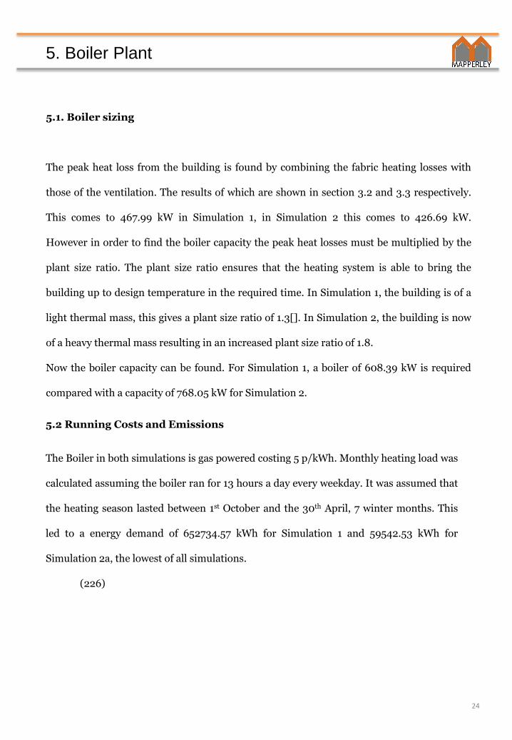
5.1. Boiler sizing
The peak heat loss from the building is found by combining the fabric heating losses with
those of the ventilation. The results of which are shown in section 3.2 and 3.3 respectively.
This comes to 467.99 kW in Simulation 1, in Simulation 2 this comes to 426.69 kW.
However in order to find the boiler capacity the peak heat losses must be multiplied by the
plant size ratio. The plant size ratio ensures that the heating system is able to bring the
building up to design temperature in the required time. In Simulation 1, the building is of a
light thermal mass, this gives a plant size ratio of 1.3[]. In Simulation 2, the building is now
of a heavy thermal mass resulting in an increased plant size ratio of 1.8.
Now the boiler capacity can be found. For Simulation 1, a boiler of 608.39 kW is required
compared with a capacity of 768.05 kW for Simulation 2.
5.2 Running Costs and Emissions
The Boiler in both simulations is gas powered costing 5 p/kWh. Monthly heating load was
calculated assuming the boiler ran for 13 hours a day every weekday. It was assumed that
the heating season lasted between 1st October and the 30th April, 7 winter months. This
led to a energy demand of 652734.57 kWh for Simulation 1 and 59542.53 kWh for
Simulation 2a, the lowest of all simulations.
(226)
24

6. Air Conditioning
6.1 Sizing the Air Conditioning System (ACS).
From the maximum cooling load, the office block’s ACS can be
sized. This was found to be 671KW. The ACS is primarily used for
cooling and is the main cooling source within the building, the only
other being the heat loss due to conduction in winter periods.
A definite volume of air was found that was required to meet the
needs of the office space, both in terms of heat gains and the fresh
air required for the occupants shown in Table 6.1.1.
The proportion of fresh air is displayed in Table 6.1.2 and
accounted for in the Psychrometric chart
Table 6.1.1
FloorRequired volume
of air (m3/s)
1 3
2-9 5.77
10 6.14
Table 6.1.2
FloorProportion of fresh
air %
1 10.67
2-9 14.21
10 13.35
6.2 Psychrometric Process
6.2.1 – Simulation 1
Figure 6.2.1.1 – Finding room point
25
6. Air Conditioning
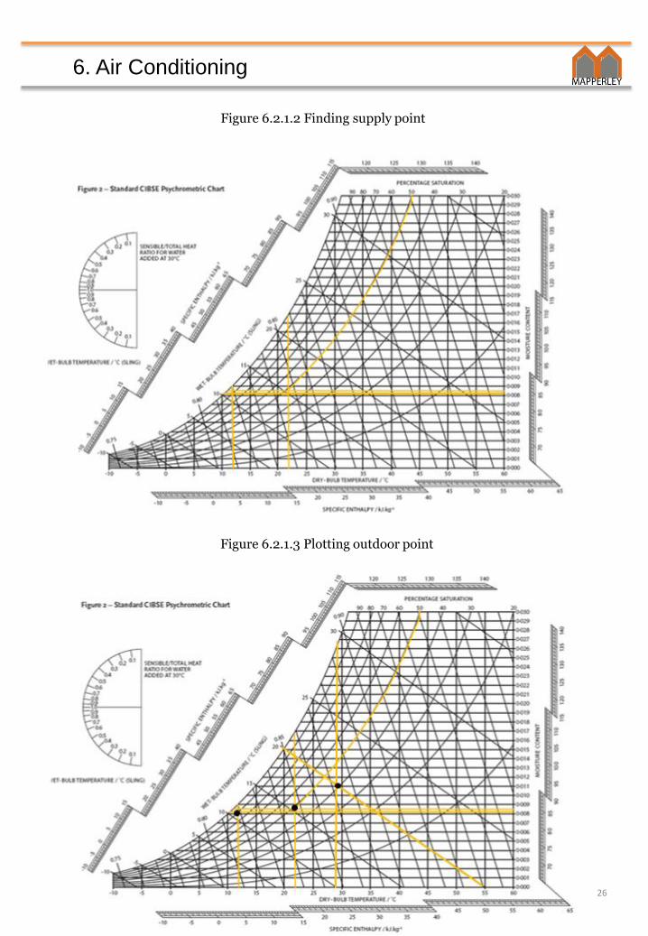
Figure 6.2.1.2 Finding supply point
Figure 6.2.1.3 Plotting outdoor point
26

6. Air Conditioning
Figure 6.2.1.4 Plotting mixing point and Final cycle
Equation 6.2.1.1, Calculating supply moisture content
𝑔𝑠 = 𝑔𝑟 −𝐿𝐻
𝐿𝑥𝑀
Where, gs is Supply Moisture Content, gr is Room Moisture Content taken from Figure 6.2.1,
LH is Latent Heat Gains (W), L is Latent Heat Vaporization Capacity (kJ/kg), M is Mass Flow
Rate (m3/s)
Example Calculation 6.2.1.1, Supply moisture content
𝑔𝑠 = 0.0085 −44.67
2450𝑥17.05
𝑔𝑠 =0.0074
27

6. Air Conditioning
6.2 - Simulation 2 – Psychrometric process with simulation 2 conditions applied
6.3 Design criterion, ACS type
The system designed for this office block is a variable air volume (VAV) air conditioning system
(ACS). It was chosen due to the varying throws from each diffuser and changes in the proportion of
air exiting each diffuser which maintains a constant volume of air being supplied to the office per
m2.
To simplify the system, minimising the number of air handling units, it was decided to set the
fresh air proportion to the maximum value of 14.21% for the whole building, with 85.79% being re-
circulated. Although this may increase building running costs as the fan will continue at a constant
rate rather than meeting the demand, it will reduce capital costs minimising the amount of
ductwork, but also provide more space within the building that would otherwise house extra ducts.
28

6. Air Conditioning
Table 6.3.1 – Advantages and Disadvantages of a VAV system
VAV System
Advantages Disadvantages
Incredibly useful in an office as the temperature can be
controlled throughout the year to meet the occupants needs.
It uses a lot of space, which is already limited in this
building
Also has the ability to vary the flow rate from the diffusers as
well as the mixing point to meet the fresh air demand
reducing running costs.
The fan-assisted terminal units can increase noise
levels potentially disrupting people working.
6.4 - ACS Mechanism, components and AHU Components
6.4.1 ACS Mechanism
The ACS mechanism is made up of 5 key areas. They are the condensing mechanism, drying
mechanism, expanding mechanism, evaporating mechanism and compressing mechanism. The
ambient air passes through the condenser into a blower motor before being passed through the
evaporator and produced as conditioned air.
6.4.2 ACS components
The components that carry out said mechanisms are the condenser fan, drier, expansion valve,
evaporator and compressor clutch.
6.4.3 AHU components
The components that make up the AHU system for the office building are the supply duct, the fan
compartment, the heating coil, the cooling coil, the filter compartment and mixing box.
29

6. Air Conditioning
6.5 - Control strategy
The air condition system will run between 1st May to 30th September, the 5 warmest months.
Since the ACS is VAV the required level of cooling to any number of zones can be controlled.
This is advantageous for periods when the building isn’t at full occupancy (7am-9am and
6pm-8pm). The air flow rates will be reduced during these periods to save on energy as the air
volume rate required will be limited.
6.6 - Gross annual running costs
To estimate the annual running cost, first the peak cooling load was found and root mean
square taken to find the average. Then the root mean square of causal heat gains was found to
calculate Pelec. The sum of these dictated the cooling load to find the total cooling demand.
Table 6.6.1, Simulation 2a Air conditioning
Pelec (kW)Hours/Y
ear
Total Demand
(Kwh)Cost (£)
Cost/m2
(£)
Emission Factor
(C02/kWh)
CO2 Cost
(KgCO2)
Cost/m2
(KgCO2)
1.14 1430 516737.74 0.1 5.29 0.49 253201.5 25.92
Table 6.6.1, Simulation 1 Air conditioning
Pelec (kW)Hours/Y
ear
Total Demand
(Kwh)Cost (£)
Cost/m2
(£)
Emission Factor
(C02/kWh)
CO2 Cost
(KgCO2)
Cost/m2
(KgCO2)
2.56 1430 955992.3 0.1 9.79 0.49 468436.2 47.96
Table 6.6.1, Simulation 2b Air conditioning
Pelec (kW)Hours/Y
ear
Total Demand
(Kwh)Cost (£)
Cost/m2
(£)
Emission Factor
(C02/kWh)
CO2 Cost
(KgCO2)
Cost/m2
(KgCO2)
2.38 1430 897045.38 0.1 9.18 0.49 253201.49 25.92
30

6. Air Conditioning
Table 6.6.1, Simulation 2c Air conditioning
Pelec (kW)Hours/Y
ear
Total Demand
(Kwh)Cost (£)
Cost/m2
(£)
Emission Factor
(C02/kWh)
CO2 Cost
(KgCO2)
Cost/m2
(KgCO2)
1.19 1430 531429.14 0.1 5.44 0.49 260400.3 26.66
Table 6.6.1, Simulation 2d Air conditioning
Pelec (kW)Hours/Y
ear
Total Demand
(Kwh)Cost (£)
Cost/m2
(£)
Emission Factor
(C02/kWh)
CO2 Cost
(KgCO2)
Cost/m2
(KgCO2)
2.43 1430 911733.76 0.1 9.33 0.49 446749.5 45.74
(448)
31
Figure 6.1.1 – 3D projection of duct layout with diffuser throw, Ground floor
Figure 6.1.2 – 3D projection of Diffuser on duct, Ground floor

7. Ventilation
7.1, Duct configuration
The first step to design the duct configuration is to obtain the noise limit of 7.5 m/s [21]. By
ensuring the velocity was less than 7.5 m/s the throw was selected using the Gilbert
nomogram for each diffuser based on geometric limitations respectively. Once the throw was
defined the layout of the diffusers were drawn using the diameters. The configuration of the
ducts was then drawn connecting each diffuser to the main duct in the best possible way to
limit duct lengths.
Figure 7.1.3 Supply for General Floor, illustrating throw of each diffuser
Figure 7.1.4 Supply for Ground Floor, Illustrating throw of each diffuser
32
7. Ventilation
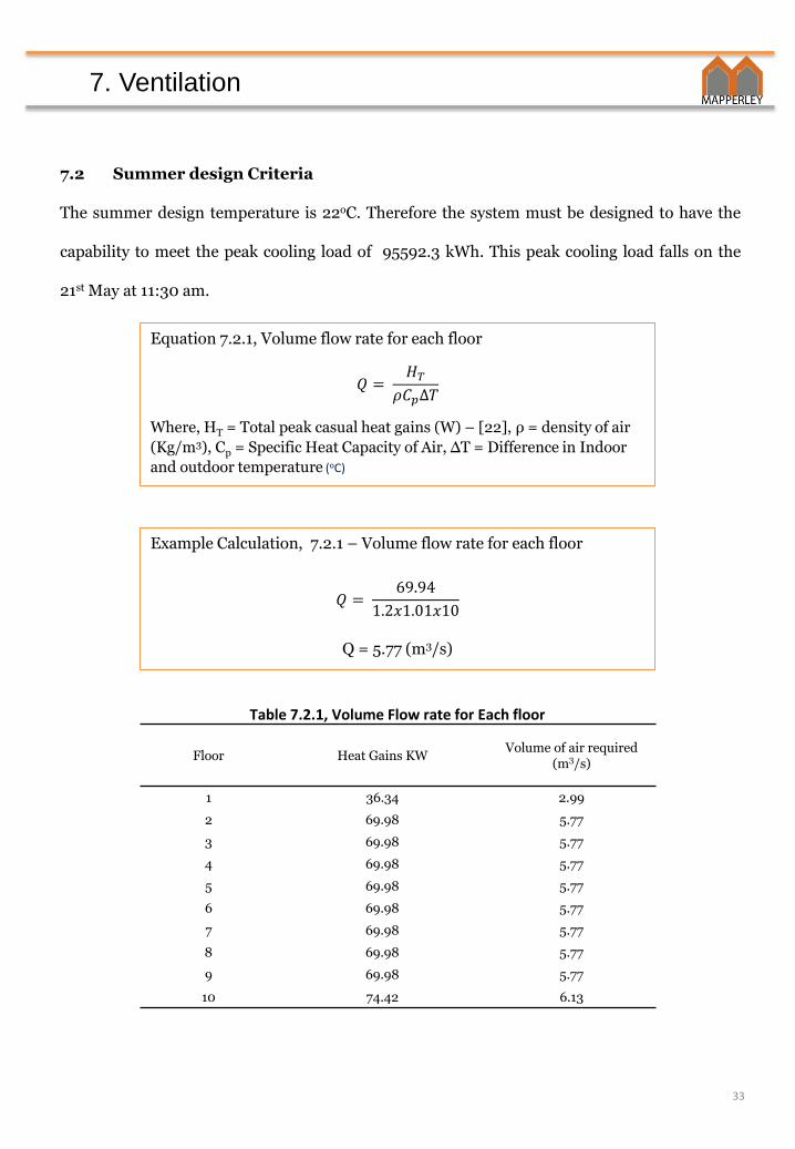
7.2 Summer design Criteria
The summer design temperature is 22oC. Therefore the system must be designed to have the
capability to meet the peak cooling load of 95592.3 kWh. This peak cooling load falls on the
21st May at 11:30 am.
Equation 7.2.1, Volume flow rate for each floor
𝑄 =𝐻𝑇𝜌𝐶𝑝∆𝑇
Where, HT = Total peak casual heat gains (W) – [22], ρ = density of air
(Kg/m3), Cp = Specific Heat Capacity of Air, ΔT = Difference in Indoor
and outdoor temperature (oC)
Example Calculation, 7.2.1 – Volume flow rate for each floor
𝑄 =69.94
1.2𝑥1.01𝑥10
Q = 5.77 (m3/s)
Table 7.2.1, Volume Flow rate for Each floor
Floor Heat Gains KWVolume of air required
(m3/s)
1 36.34 2.99
2 69.98 5.77
3 69.98 5.77
4 69.98 5.77
5 69.98 5.77
6 69.98 5.77
7 69.98 5.77
8 69.98 5.77
9 69.98 5.77
10 74.42 6.13
33
7. Ventilation
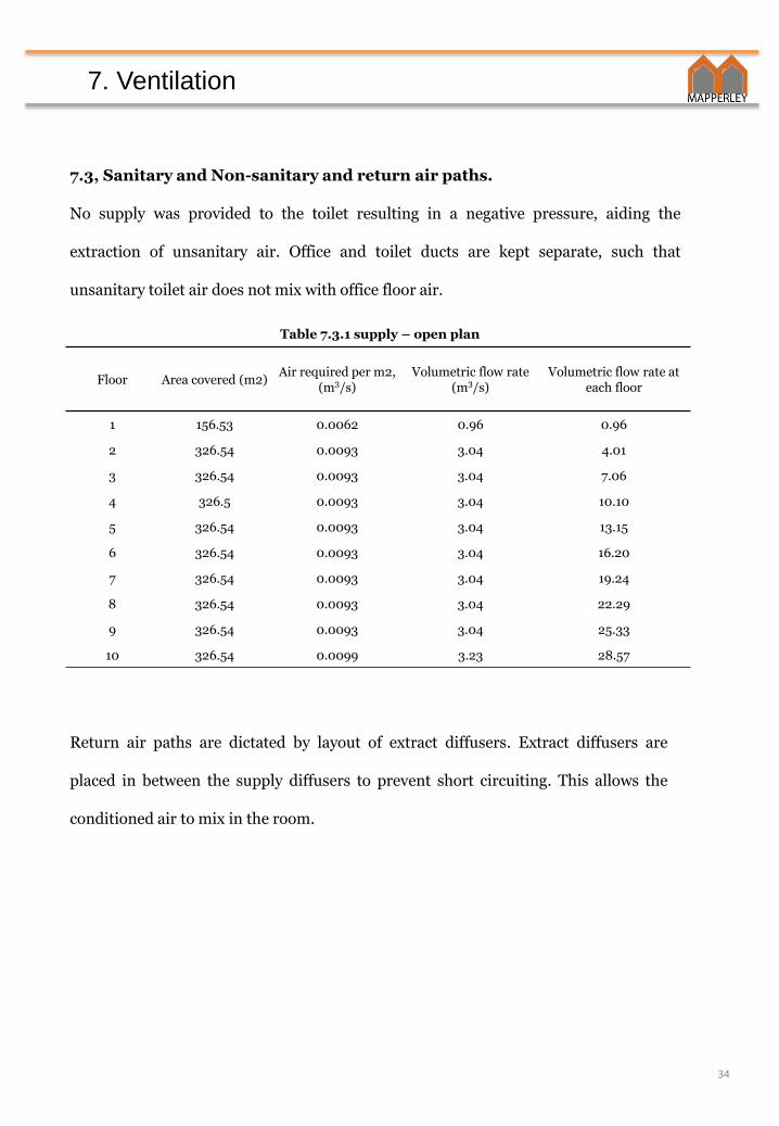
7.3, Sanitary and Non-sanitary and return air paths.
No supply was provided to the toilet resulting in a negative pressure, aiding the
extraction of unsanitary air. Office and toilet ducts are kept separate, such that
unsanitary toilet air does not mix with office floor air.
Table 7.3.1 supply – open plan
Floor Area covered (m2)Air required per m2,
(m3/s)Volumetric flow rate
(m3/s)Volumetric flow rate at
each floor
1 156.53 0.0062 0.96 0.96
2 326.54 0.0093 3.04 4.01
3 326.54 0.0093 3.04 7.06
4 326.5 0.0093 3.04 10.10
5 326.54 0.0093 3.04 13.15
6 326.54 0.0093 3.04 16.20
7 326.54 0.0093 3.04 19.24
8 326.54 0.0093 3.04 22.29
9 326.54 0.0093 3.04 25.33
10 326.54 0.0099 3.23 28.57
Return air paths are dictated by layout of extract diffusers. Extract diffusers are
placed in between the supply diffusers to prevent short circuiting. This allows the
conditioned air to mix in the room.
34

7. Ventilation
Figure 7.2.1 Extract layout for General Floor
Figure 7.2.2 Extract Layout for Ground Floor
35
7. Ventilation
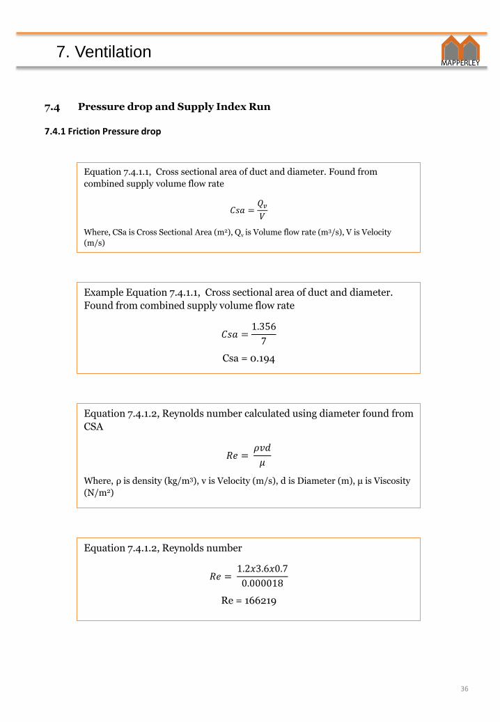
7.4 Pressure drop and Supply Index Run
7.4.1 Friction Pressure drop
Equation 7.4.1.1, Cross sectional area of duct and diameter. Found from
combined supply volume flow rate
𝐶𝑠𝑎 =𝑄𝑣𝑉
Where, CSa is Cross Sectional Area (m2), Qv is Volume flow rate (m3/s), V is Velocity
(m/s)
Example Equation 7.4.1.1, Cross sectional area of duct and diameter.
Found from combined supply volume flow rate
𝐶𝑠𝑎 =1.356
7
Csa = 0.194
Equation 7.4.1.2, Reynolds number calculated using diameter found from
CSA
𝑅𝑒 =𝜌𝑣𝑑
𝜇
Where, ρ is density (kg/m3), v is Velocity (m/s), d is Diameter (m), μ is Viscosity
(N/m2)
Equation 7.4.1.2, Reynolds number
𝑅𝑒 =1.2𝑥3.6𝑥0.7
0.000018
Re = 166219
36

7. Ventilation
Equation 7.4.1.3, The Haaland Equation for turbulent flow, to find friction factor, λ
𝜆 = (1
(−1.8log[6.9𝑅𝑒+ (
𝑘𝑑3.71)1.11]
)2
Where Re = Reynolds number, k = Roughness Coefficient assuming steel duct
= 0.09[23]. d = diameter
Equation 7.4.1.3, The Haaland Equation for turbulent flow, λ
𝜆 = (1
(−1.8log[6.9166219
+ (
0.090.73.71)1.11]
)2
λ = 0.022
Equation 7.4.1.4, Pressure drop per unit length
𝛥𝑃/𝑚 =𝜆𝜌𝑣
2𝑑
Equation 7.4.1.4, Pressure Drop per unit length
𝛥𝑃/𝑚 =0.022𝑥1.2𝑥3.62
2𝑥0.7
𝛥𝑃/𝑚 = 0.25Pa/m
37

7. Ventilation
Equation 7.4.1.5, Pressure drop due to Friction
∆𝑃𝐹𝑟𝑖𝑐𝑡𝑖𝑜𝑛= ∆𝑃/𝑚𝑙
Where, l = length of duct (m)
Example Calculation7.4.1.5, Pressure drop due to Friction
∆𝑃𝐹𝑟𝑖𝑐𝑡𝑖𝑜𝑛= 0.25𝑥3.6
∆𝑃𝐹𝑟𝑖𝑐𝑡𝑖𝑜𝑛= 0.9Pa
7.4.2 Pressure Loss due to component
Equation 7.4.2.1, Alternative CSA ratios used to calculate ζ (Component
Loss Coefficient) for contraction.
𝜁 = 0.5[ 1 −𝐴2𝐴1
0.75
]
Where, A2 = Cross sectional area after Contraction, A1 = Cross sectional area
before Contraction.
Example Equation 7.4.2.1, Alternative CSA ratios used to calculate ζ
(Component Loss Coefficient) for contraction.
𝜁 = 0.5[ 1 − 0.6 0.75]
𝜁 = 0.25
38
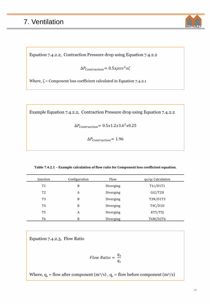
7. Ventilation
Equation 7.4.2.2, Contraction Pressure drop using Equation 7.4.2.2
∆𝑃𝐶𝑜𝑛𝑡𝑟𝑎𝑐𝑡𝑖𝑜𝑛= 0.5𝑥𝜌𝑥𝑣2𝑥𝜁
Where, ζ = Component loss coefficient calculated in Equation 7.4.2.1
Example Equation 7.4.2.2, Contraction Pressure drop using Equation 7.4.2.2
∆𝑃𝐶𝑜𝑛𝑡𝑟𝑎𝑐𝑡𝑖𝑜𝑛= 0.5𝑥1.2𝑥3.62𝑥0.25
∆𝑃𝐶𝑜𝑛𝑡𝑟𝑎𝑐𝑡𝑖𝑜𝑛= 1.96
Table 7.4.2.1 – Example calculation of flow ratio for Component loss coefficient equation.
Junction Configuration Flow qs/qc Calculation
T1 B Diverging T1c/D1T1
T2 A Diverging Gt2/T2H
T3 B Diverging T3N/D1T3
T4 B Diverging T4C/D1D
T5 A Diverging KT5/T5J
T6 B Diverging T6M/D2T6
Equation 7.4.2.3, Flow Ratio
𝐹𝑙𝑜𝑤 𝑅𝑎𝑡𝑖𝑜 =𝑞𝑠𝑞𝑐
Where, qs = flow after component (m3/s) , qc = flow before component (m3/s)
39

7. Ventilation
Example Equation 7.4.2.3 Flow Ratio
𝐹𝑙𝑜𝑤 𝑅𝑎𝑡𝑖𝑜 =1.35
4.4
𝐹𝑙𝑜𝑤 𝑅𝑎𝑡𝑖𝑜 = 0.3
Flow ratio of 0.3 then equates to a value of ζ = 0.18[24]
Equation 7.4.2.4, Component Pressure Drop
∆𝑃𝐶𝑜𝑚𝑝𝑜𝑛𝑒𝑛𝑡= 0.5𝑥𝜁𝑥𝜌𝑥𝑣2
Example Calculation 7.4.2.4, Component Pressure Drop
∆𝑃𝐶𝑜𝑚𝑝𝑜𝑛𝑒𝑛𝑡= 0.5𝑥0.18𝑥1.2𝑥3.62
∆𝑃𝐶𝑜𝑚𝑝𝑜𝑛𝑒𝑛𝑡= 1.4
40

7. Ventilation
Equation 7.4.2.5, Total Pressure drop
∆𝑃𝑇𝑜𝑡𝑎𝑙= ∆𝑃𝐹𝑟𝑖𝑐𝑡𝑖𝑜𝑛+∆𝑃𝐶𝑜𝑛𝑡𝑟𝑎𝑐𝑡𝑖𝑛+∆𝑃𝐶𝑜𝑚𝑝𝑜𝑛𝑒𝑛𝑡
Example Calculation 7.4.2.5 Total Pressure drop
∆𝑃𝑇𝑜𝑡𝑎𝑙=0.9+1.95+1.4
∆𝑃𝑇𝑜𝑡𝑎𝑙= 4.26
The supply index run is obtained as the run with the greatest ΔP which is
from the AHU on the 10th floor to the ground floor onto diffuser p in Duct
2 and has a pressure drop of 1051.169 Pa.
7.5 – Supply Diffuser choice
Table 7.5.1 – Data for Gilbert Nomogram
Branch Velocity (m/s) Throw (m) Volume flow rate (m3/s)
I 2.86 3.3 0.32
41

7. Ventilation
Figure 7.5.1 - Example nomogram used to define size of supply
diffuser.
Table 7.5.2 – Results from nomogram for diffuser dimensions
Grille I
Width (mm) 375
Height (mm) 325
42
7. Ventilation
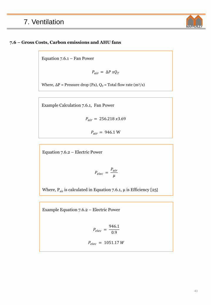
7.6 – Gross Costs, Carbon emissions and AHU fans
Equation 7.6.1 – Fan Power
𝑃𝑎𝑖𝑟 = ∆𝑃 𝑥𝑄𝑇
Where, ΔP = Pressure drop (Pa), QT = Total flow rate (m3/s)
Example Calculation 7.6.1, Fan Power
𝑃𝑎𝑖𝑟 = 256.218 𝑥3.69
𝑃𝑎𝑖𝑟 = 946.1W
Equation 7.6.2 – Electric Power
𝑃𝑒𝑙𝑒𝑐 =𝑃𝑎𝑖𝑟𝜇
Where, Pair is calculated in Equation 7.6.1, μ is Efficiency [25]
Example Equation 7.6.2 – Electric Power
𝑃𝑒𝑙𝑒𝑐 =946.1
0.9
𝑃𝑒𝑙𝑒𝑐 = 1051.17𝑊
43

7. Ventilation
Table 7.6.1 Supply Electric Power
Index run – Supply
Duct Area ΔP Qt Pair μ Pelec
2 T6 - P 325.55 2.64 858.17 0.9 953.52
1 T4 - G 113.60 2.48 281.24 0.9 312.49
1 Toilet 899.59 0.02 21.49 0.9 23.87
2 Toilet 867.51 0.05 39.94 0.9 44.38
Table 7.6.2 Extract Electric Power
Index run - Extract
Duct Area ΔP Qt Pair μ Pelec
1 T1 - I 111.08 2.56 283.8 0.9 315.35
2 T4 - s 97.6 5.28 515.28 0.9 572.54
1 Toilet 899.94 0.02 21.49 0.9 23.89
2 Toilet 866.79 0.05 39.91 0.9 44.34
The number of AHU fans corresponds to the number of extract and supply run
systems which is 6. Therefore there will be 6 AHU fans.
7.6.1 Cost Considerations
In order to minimise gross running cost, components in the duct work are kept to
a minimum. Straight paths are augmented rather than bent. Total length is
restricted to minimise pressure drop and power needed. (299)
44

8. Sensitivity Analysis
Figure 8.1, Energy Proportions, Simulation 1
0
500000
1000000
1500000
2000000
1 2a 2b 2c 2d
Ene
rgy
De
man
d (
kWh
)
Simulation
Fan EnergyDemand (kWh)
Cooling Demand(kWh)
HeatingDemand (kWh)
HeatingDemand (kWh)
CoolingDemand (kWh)
Fan EnergyDemand (kWh)
HeatingDemand (kWh)
CoolingDemand (kWh)
Fan EnergyDemand (kWh)
HeatingDemand (kWh)
CoolingDemand (kWh)
Fan EnergyDemand (kWh)
HeatingDemand (kWh)
CoolingDemand (kWh)
Fan EnergyDemand (kWh)
HeatingDemand (kWh)
CoolingDemand (kWh)
Fan EnergyDemand (kWh)
Figure 8.2, Energy Proportions, Simulation 2a
Figure 8.3, Energy Proportions, Simulation 2b
Figure 8.4, Energy Proportions, Simulation 2c
Figure 8.5, Energy Proportions, Simulation 2d
Figure 8.6, Annual Energy Demand Comparison
Figures 8.1 to 8.6 show the proportion of energy demand for Heating, Cooling and Fan
power for each simulation and a comparison of the 5 simulations. The figures show
that the greatest reductions in energy demand come from reducing cooling load. (41)
45

8. Sensitivity Analysis
8.1. Heating
The lowest heating demand is shown in Simulations 2a and 2b, a decrease of 9% on
the largest value. (19)
Table 8.1.1, Heating Demands
SimulationHeating Demand
(kWh)
1 652734.57
2a 595423.53
2b 595423.53
2c 652734.57
2d 652734.57
This is a result of the winter internal temperatures being decreased by 2°C. By
reducing winter internal temperatures there is an associated heat loss reduction
due to the decreased temperature difference - by Equations 3.1 and 3.2. (37)
8.2. Cooling
Simulation 1 exhibits the greatest cooling demand due to the short lag time. Heat
gains are transmitted directly into the building during occupied hours and these
this offset by the cooling load. In simulations 2.n increased lag time means the
largest sol-air gains do not affect the internal temperature until after occupied
hours, resulting in a cooling load decrease of 5%. Additionally complete solar
shading removes solar transmission which results in decreased cooling demand in
Simulations 2a and 2b of an additional 40%. (83)
46

8. Sensitivity Analysis
Table 8.2.1, Cooling Demand
SimulationCooling Demand
(kWh)
1 952330.75
2a 515104.65
2b 893636.07
2c 529725.62
2d 908257.04
8.3. Fan Energy Demand
The fan runs constantly during the heating and cooling system in order to provide the
fresh air requirement for the room occupants. In summer it runs at an increased rate
to accommodate for the increased heat gain. Therefore the required fan energy
decreases proportional to the cooling demand.
(48)
Table 8.3.1, Fan Energy Demand
SimulationFan Energy Demand
(kWh)
Heating Season 848.53
1 3661.54
2a 1663.09
2b 3409.30
2c 1703.52
2d 3476.73
8.4. Total Energy Demand
The greatest energy demand occurs for Simulation 1 due to it’s low thermal density,
large temperature difference between indoor and outdoor and high solar exposure.
Simulation 2a has the lowest total energy demand (31% less).
(35)
47
8. Sensitivity Analysis
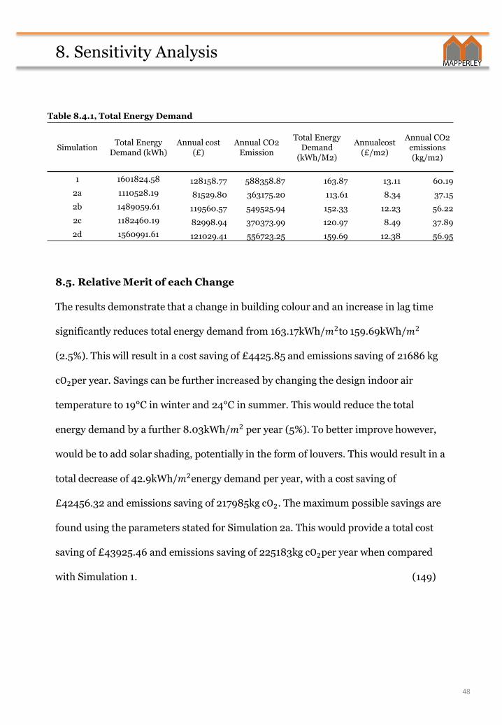
8.5. Relative Merit of each Change
The results demonstrate that a change in building colour and an increase in lag time
significantly reduces total energy demand from 163.17kWh/𝑚2to 159.69kWh/𝑚2
(2.5%). This will result in a cost saving of £4425.85 and emissions saving of 21686 kg
cO2per year. Savings can be further increased by changing the design indoor air
temperature to 19°C in winter and 24°C in summer. This would reduce the total
energy demand by a further 8.03kWh/𝑚2 per year (5%). To better improve however,
would be to add solar shading, potentially in the form of louvers. This would result in a
total decrease of 42.9kWh/𝑚2energy demand per year, with a cost saving of
£42456.32 and emissions saving of 217985kg cO2. The maximum possible savings are
found using the parameters stated for Simulation 2a. This would provide a total cost
saving of £43925.46 and emissions saving of 225183kg cO2per year when compared
with Simulation 1. (149)
Table 8.4.1, Total Energy Demand
SimulationTotal Energy
Demand (kWh)Annual cost
(£)Annual CO2
Emission
Total Energy Demand
(kWh/M2)
Annualcost (£/m2)
Annual CO2 emissions (kg/m2)
1 1601824.58 128158.77 588358.87 163.87 13.11 60.19
2a 1110528.19 81529.80 363175.20 113.61 8.34 37.15
2b 1489059.61 119560.57 549525.94 152.33 12.23 56.22
2c 1182460.19 82998.94 370373.99 120.97 8.49 37.89
2d 1560991.61 121029.41 556723.25 159.69 12.38 56.95
48

9. Fire Safety
9.1 Compartmentalisation
Each storey is separated by fire resistant floors and doors.
Figure 9.1.1 shows the fire protected shaft housing the ducts
and the stairs. The fire doors will match the separating
construction and so are maximum 75mm.
From Table A1[26], the firefighting shaft exterior should
provide at least 120 minutes. Table 12[27] shows there is no
limit on floor area. As both stairs are entered at each level
via a protected lobby, both stairs can be assumed available.
Figure 9.1.1 - Fire protected shaft (red)
Equation 9.2.1 Maximum Distance to nearest fire exit .
14.49 + 6.6 + 15.38 = 36.47𝑚
2 fire doors should be added on each side of the service area [28]
49
9.2 Horizontal escapeFigure 9.2.1, Suggested Fire escape door example
Figure 9.2.2, Maximum travel distances in one direction, Ground Floor

9. Fire Safety
Figure 9.2.3 – Maximum travel distance in multiple directions on floor 1-9
Figure 9.2.4 – Maximum travel distance in one direction on floor 1-9
Equation 9.2.2 Maximum Distance to nearest fire exit when travel is possible in multiple directions
11.76 + 4.5 + 4.5 = 20.76𝑚
Equation 9.2.3 Maximum Distance to
nearest fire exit when travel is possible in
one direction.
15.48 + 4.5 = 19.98
Where, this results in another fire door
being installed on each stairwell50
Figure 9.2.5, Suggested Fire escape door example, Typical Upper Floor.
9. Fire Safety
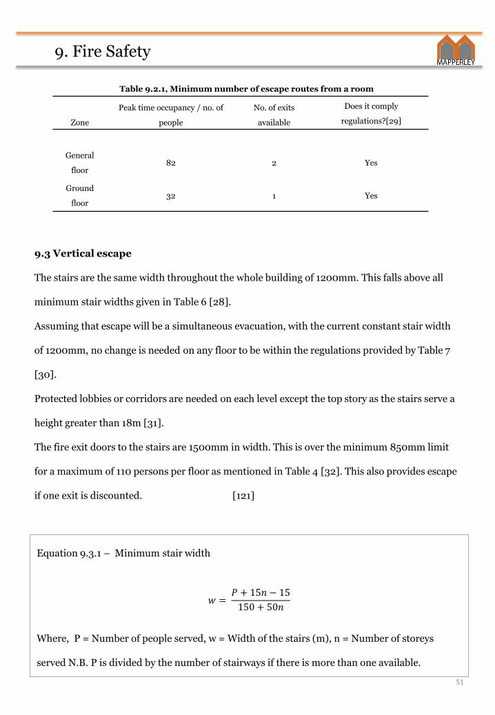
Table 9.2.1, Minimum number of escape routes from a room
Zone
Peak time occupancy / no. of
people
No. of exits
available
Does it comply
regulations?[29]
General
floor82 2 Yes
Ground
floor32 1 Yes
9.3 Vertical escape
The stairs are the same width throughout the whole building of 1200mm. This falls above all
minimum stair widths given in Table 6 [28].
Assuming that escape will be a simultaneous evacuation, with the current constant stair width
of 1200mm, no change is needed on any floor to be within the regulations provided by Table 7
[30].
Protected lobbies or corridors are needed on each level except the top story as the stairs serve a
height greater than 18m [31].
The fire exit doors to the stairs are 1500mm in width. This is over the minimum 850mm limit
for a maximum of 110 persons per floor as mentioned in Table 4 [32]. This also provides escape
if one exit is discounted. [121]
Equation 9.3.1 – Minimum stair width
𝑤 =𝑃 + 15𝑛 − 15
150 + 50𝑛
Where, P = Number of people served, w = Width of the stairs (m), n = Number of storeys
served N.B. P is divided by the number of stairways if there is more than one available.
51
9. Fire Safety
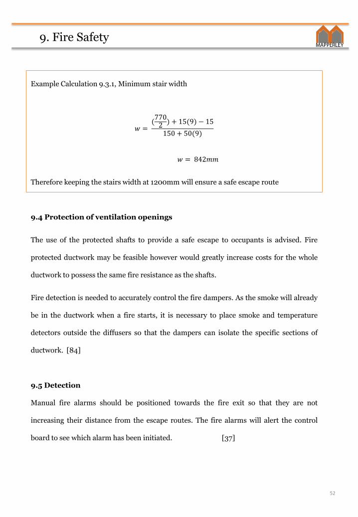
Example Calculation 9.3.1, Minimum stair width
𝑤 =(7702 ) + 15(9) − 15
150 + 50(9)
𝑤 = 842𝑚𝑚
Therefore keeping the stairs width at 1200mm will ensure a safe escape route
9.4 Protection of ventilation openings
The use of the protected shafts to provide a safe escape to occupants is advised. Fire
protected ductwork may be feasible however would greatly increase costs for the whole
ductwork to possess the same fire resistance as the shafts.
Fire detection is needed to accurately control the fire dampers. As the smoke will already
be in the ductwork when a fire starts, it is necessary to place smoke and temperature
detectors outside the diffusers so that the dampers can isolate the specific sections of
ductwork. [84]
9.5 Detection
Manual fire alarms should be positioned towards the fire exit so that they are not
increasing their distance from the escape routes. The fire alarms will alert the control
board to see which alarm has been initiated. [37]
52
9. Fire Safety
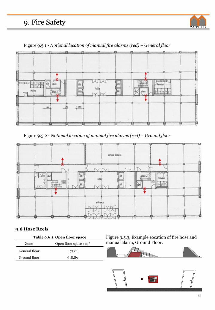
Figure 9.5.1 - Notional location of manual fire alarms (red) – General floor
Figure 9.5.2 - Notional location of manual fire alarms (red) – Ground floor
9.6 Hose Reels
Table 9.6.1, Open floor space
Zone Open floor space / m²
General floor 477.61
Ground floor 618.89
53
Figure 9.5.3, Example eocation of fire hose and manual alarm, Ground Floor.

9. Fire Safety
There must be one hose per 800 m2 of floor space and it must also have a water supply
which is at least 24ls-1 to produce a 6m jet. The hose reel needs to be capable of reaching
within 6m of every part of the space [33]. The hose reels be a length of 40m.
[57]
Figure 9.6.1 - Notional location of hoses (green) – Ground floor
Figure 9.6.2 - Notional location of hoses (green) – General floor
54

9. Fire Safety
9.7 Sprinklers
Office building must possess sprinklers[34]. Both systems require risers which will be wet in the
summer and dry in the winter for when the ambient temperature drops below o°C
Table 9.7.1, Spacing between sprinklers
Maximum spacing between sprinklers 4.572m [35]
Minimum spacing between sprinklers 1.829m [35]
The sprinkler system for each floor will consist of risers (blue), main distribution pipe (red),
range pipes (green), arm pipes (black) and sprinkler heads (crosses). The sprinkler heads will
operate at a temperature of 65°C. This occurs via a fusible link that melts at 65°C and opens
the sprinkler head. The flow of water sets of the main fire alarm system and will alert the
control board which arm pipe(s) has been affected to locate the fire quickly.
Figure 9.7.1 Notional location of sprinkler system – General floor
55

9. Fire Safety
Figure 9.7.2 Notional location of sprinkler system – Ground floor
Table 9.8.1, Landing valve specification
Landing valve minimum height above
finished floor 750mm [33]
Bore width 150mm [33]
Figure 9.8.3 Illustrating drop pipes (orange)
56
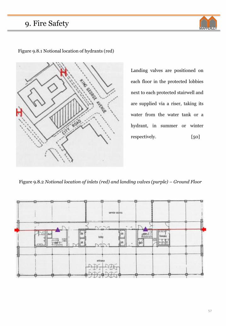
9.8 Hydrants, Risers and Landing Valves
9. Fire Safety
Figure 9.8.1 Notional location of hydrants (red)
Landing valves are positioned on
each floor in the protected lobbies
next to each protected stairwell and
are supplied via a riser, taking its
water from the water tank or a
hydrant, in summer or winter
respectively. [50]
Figure 9.8.2 Notional location of inlets (red) and landing valves (purple) – Ground Floor
57
9. Fire Safety
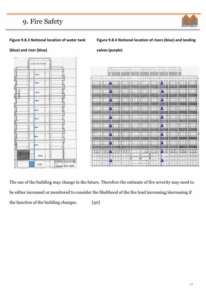
Figure 9.8.3 Notional location of water tank
(blue) and riser (blue)
Figure 9.8.4 Notional location of risers (blue) and landing
valves (purple)
The use of the building may change in the future. Therefore the estimate of fire severity may need to
be either increased or monitored to consider the likelihood of the fire load increasing/decreasing if
the function of the building changes. [50]
58

10. Vertical Transport
10.1 Background
‘First Model’ of mathematical formula described [36] provides ‘satisfactory solution for 90-95% of
[vertical transport] designs’. For this reason it is the best model to gain an estimate of the ability of
the current lift shafts to handle the building occupancy. Following are the equations used and a
description of the method. Table 10.1.1 shows the terms and definitions for this section.
Equation 10.1.1, Performance Time (T).
𝑇 = 𝑡𝑓 1 + 𝑡𝑠𝑑 + 𝑡𝑐 + 𝑡𝑜 − 𝑡𝑎𝑑
Equation 10.1.2, Floor Transit Time (𝒕𝒗).
𝑡𝑣 = 𝑑𝑓/𝑣
Equation 10.1.3, Average Interfloor Distance 𝑫𝑻)
𝑑𝑓 =𝐷𝑇𝑁
Equation 10.1.4, Average Highest Reversal Floor (H).
𝐻 = 𝑁 −
𝑖=1
𝑁−1𝑖
𝑁
6.3
Equation 10.1.5 – Average Number Of Stops (S).
𝑆 = 𝑁 1 − 1 −1
𝑁
𝑃
Equation 10.1.6, Round Trip Time (RTT).
𝑅𝑇𝑇 = 2𝐻𝑡𝑣 + 𝑆 + 1 𝑇 − 𝑡𝑣 + 2𝑃𝑡𝑝
Equation 10.1.7, Up-peak Interval (UPPINT).
𝑈𝑃𝑃𝐼𝑁𝑇 =𝑅𝑇𝑇
𝐿59
10.2 Method

10. Vertical Transport
Equation 10.1.8, Up-peak Handling Capacity (UPPHC).
𝑈𝑃𝑃𝐻𝐶 =300𝑃
𝑈𝑃𝑃𝐼𝑁𝑇/𝑈
Equation 10.1.9, Percentage Population Served (%POP).
%𝑃𝑂𝑃 =𝑈𝑃𝑃𝐻𝐶𝑥100
𝑈𝑃𝑃𝐼𝑁𝑇
Equation 10.1.10 – Average Number Of Passengers
𝑃 = 0.8𝐴𝐶
Table 10.1.1 - Terms and Definitions.
Term Definition
tfAverage single floor flight time (s)
tsd Start delay (s)
to Door opening time (s)
tc Door closing time (s)
tad
Advanced door openining time (s). i.e. overlap of lift levelling and door opening mechanisms
DtTotal travel distance from main terminal to highest served floor
N Number of served floors
L Number of lifts
AC Actual capacity of the lift
Table 10.1.2 - Assumptions
Assumptions:
No Manufacturers Data for to, tc,
tsd, tad,
Average passenger transfer time
is 1.2s [41]
i.e. no elderly and people in
moderate rush
Centre opening lift doors
Figure 10.1 – Showing centre opening doors and landing call system.
60
10. Vertical Transport
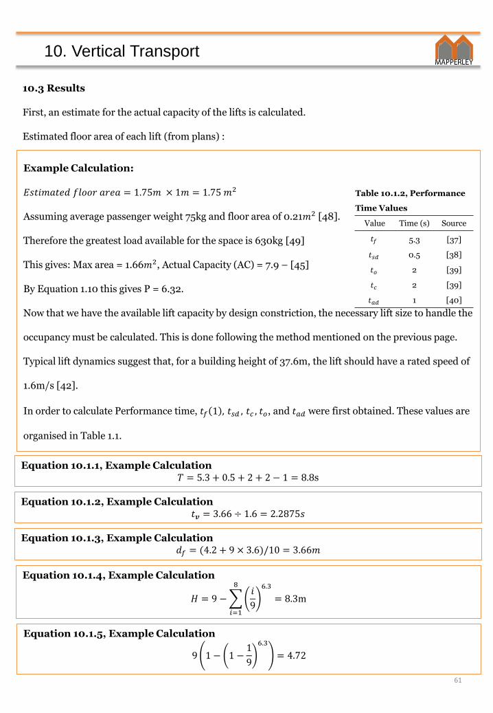
10.3 Results
First, an estimate for the actual capacity of the lifts is calculated.
Estimated floor area of each lift (from plans) :
Equation 10.1.1, Example Calculation𝑇 = 5.3 + 0.5 + 2 + 2 − 1 = 8.8s
Equation 10.1.3, Example Calculation𝑑𝑓 = (4.2 + 9 × 3.6)/10 = 3.66𝑚
Equation 10.1.4, Example Calculation
𝐻 = 9 −
𝑖=1
8𝑖
9
6.3
= 8.3m
Equation 10.1.2, Example Calculation𝑡𝒗 = 3.66 ÷ 1.6 = 2.2875𝑠
Equation 10.1.5, Example Calculation
9 1 − 1 −1
9
6.3
= 4.72
Table 10.1.2, Performance
Time Values
Value Time (s) Source
𝑡𝑓 5.3 [37]
𝑡𝑠𝑑 0.5 [38]
𝑡𝑜 2 [39]
𝑡𝑐 2 [39]
𝑡𝑎𝑑 1 [40]
Example Calculation:
𝐸𝑠𝑡𝑖𝑚𝑎𝑡𝑒𝑑 𝑓𝑙𝑜𝑜𝑟 𝑎𝑟𝑒𝑎 = 1.75𝑚 × 1𝑚 = 1.75 𝑚2
Assuming average passenger weight 75kg and floor area of 0.21𝑚2 [48].
Therefore the greatest load available for the space is 630kg [49]
This gives: Max area = 1.66𝑚2, Actual Capacity (AC) = 7.9 – [45]
By Equation 1.10 this gives P = 6.32.
Now that we have the available lift capacity by design constriction, the necessary lift size to handle the
occupancy must be calculated. This is done following the method mentioned on the previous page.
Typical lift dynamics suggest that, for a building height of 37.6m, the lift should have a rated speed of
1.6m/s [42].
In order to calculate Performance time, 𝑡𝑓 1 , 𝑡𝑠𝑑 , 𝑡𝑐 , 𝑡𝑜, and 𝑡𝑎𝑑 were first obtained. These values are
organised in Table 1.1.
61
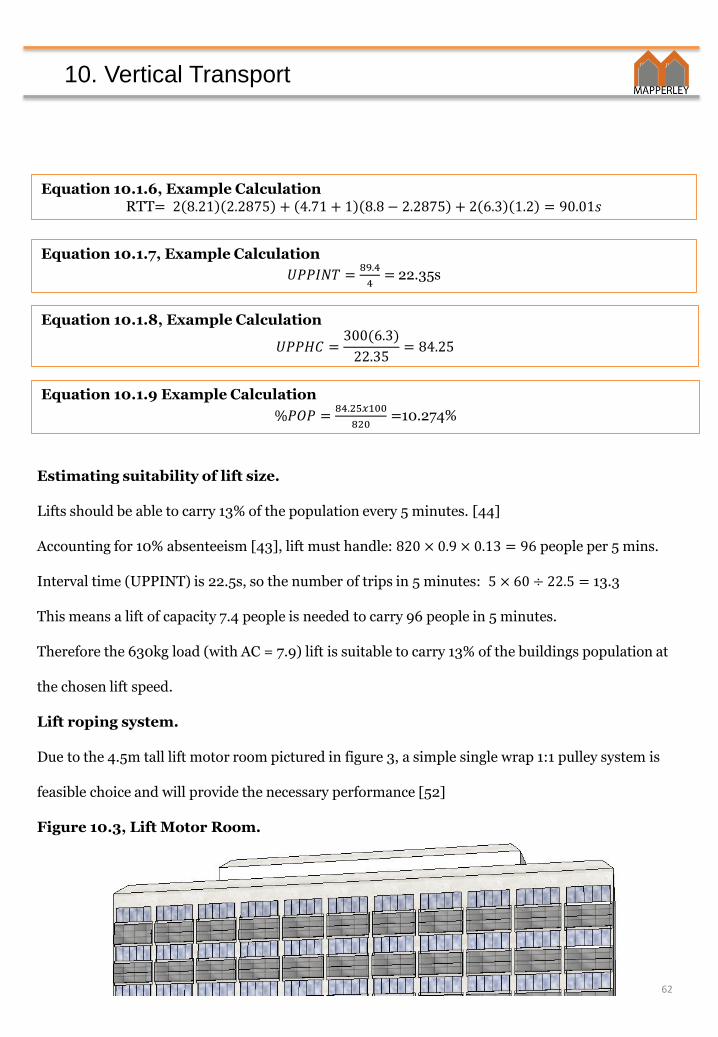
10. Vertical Transport
Estimating suitability of lift size.
Lifts should be able to carry 13% of the population every 5 minutes. [44]
Accounting for 10% absenteeism [43], lift must handle: 820 × 0.9 × 0.13 = 96 people per 5 mins.
Interval time (UPPINT) is 22.5s, so the number of trips in 5 minutes: 5 × 60 ÷ 22.5 = 13.3
This means a lift of capacity 7.4 people is needed to carry 96 people in 5 minutes.
Therefore the 630kg load (with AC = 7.9) lift is suitable to carry 13% of the buildings population at
the chosen lift speed.
Lift roping system.
Due to the 4.5m tall lift motor room pictured in figure 3, a simple single wrap 1:1 pulley system is
feasible choice and will provide the necessary performance [52]
Figure 10.3, Lift Motor Room.
Equation 10.1.6, Example CalculationRTT= 2 8.21 2.2875 + 4.71 + 1 8.8 − 2.2875 + 2 6.3 1.2 = 90.01𝑠
Equation 10.1.8, Example Calculation
𝑈𝑃𝑃𝐻𝐶 =300(6.3)
22.35= 84.25
Equation 10.1.7, Example Calculation
𝑈𝑃𝑃𝐼𝑁𝑇 =89.4
4= 22.35s
Equation 10.1.9 Example Calculation
%𝑃𝑂𝑃 =84.25𝑥100
820=10.274%
62

10. Vertical Transport
10.4 Additional information and analysis
The calculated values imply a suitable vertical transport design. In addition to this, having 2.5 lifts per
floor and 22.5s interval time imply ‘above average’ and ‘very good’ quality of service (QOS)
respectively [51]. Also, the orientation of the lift group complies with recommended layouts [45] (See
Figure 10.2)
However, this design does not consider access to the basement. The RTT can be expected to increase
by 15s per lift in serving one basement floor [46]. Since it is suggested that all lifts in one group should
serve the same floors this would result in a dramatic increase in RTTINT; and increase necessary
capacity from 7.4 to 8.5. Resulting in a lift size greater than the available area and decreased QOS.
Although increasing the lift shaft size this would increase capital cost, it would also allow for future
population increase and allow the lifts to comply with firefighting and Disability access lifts codes.
These codes suggest a lift size of no smaller than 1100mm by 1400mm. [47]
It is also advised that offices have a lift size of no less than 1000kg except in special circumstances
[52]. For these reasons it should be suggested that the architect increases the size of the lift shafts to
allow a 1000kg 1100mm by 1400mm lift.
Figure 10.2 – Showing lift group.
63

Conclusion
.
Through the running of 5 simulations with varying combinations of conditions and
said analysis of these conditions, the following sets of findings and
recommendations can be concluded.
• The heating demand can be reduced by decreasing the design internal
temperature. However the heating demand is unaffected by material properties
such at lag time and decrement factor.
• Whilst the boiler must be designed for extreme conditions, in reality the majority
of heat loss would be offset by casual and sensible heat gains. This would also
reduce the annual energy demand of the building significantly.
• The physical changes that reduced the total cooling load are ranked in order of
effectiveness below:
1) Complete solar shading,
2) Higher thermal mass and light colour in the external façade,
3) Increased set-point indoor summer temperatures
These changes all reduce the cooling load significantly, with solar shading being at
least 4 times more effective than the other changes.
• The current vertical transport system is inadequate to meet current UK
regulation for disabled and fire access and would benefit from and enlarged lift
shaft.
• Additional fire escapes are necessary in order to reduce the maximum travel
distance in the event of a fire.
• The vertical duct shaft must be enlarged in order to occupy the ducting.
(208)
64

References
[1] British Council for Offices. Occupier Density Study, 2013; Figure 2
[2] The Chartered Institution of Building Services Engineers. CIBSE Guide A, 2015; Section 1.5, Table 1.5
[3] HM Government, Approved document F, 2000; Section 6.8, Table 6.1A
[4] HM Government, Approved document L2A, 2010; Section 4.3.2, Table 4
[5] HM Government, Approved document L1, 2002; Section 1.35
[6] The Chartered Institution of Building Services Engineers. CIBSE Guide B, 2015; Table 4.19
[7] The Chartered Institution of Building Services Engineers. CIBSE Guide F, 2015; Table 12.3-12.7
[8] Chartered Institution of Building Services Engineering, CIBSE Guide A, 2015, Table 2.5
[9] Chartered Institution of Building Services Engineering, CIBSE Guide A, 2015, Table 1.5.
[10] HM Government. Approved Document L2A, 2010; Section 2.41, Table 3
[11] The Chartered Institution of Building Services Engineers. CIBSE Guide A, 2015; Section 1.5, Table 1.5
[12] The Chartered Institution of Building Services Engineers. CIBSE Guide A, 2015; Section 2.8.4, Table2.14
[13] The Chartered Institution of Building Services Engineers. CIBSE Guide A, 2015; Table 5.19
[14] The Chartered Institution of Building Services Engineers. CIBSE Guide A, 2015; Section 2.8.4, Table 2.14 (g)
[15] London Office Buildings. London Office Buildings Tender Specifications, 2016; Section 3
[16] The Chartered Institution of Building Services Engineers. CIBSE Guide A, 2015; Section 4.2.3
[17] The Chartered Institution of Building Services Engineers. CIBSE Guide A, 2015; Table 4.19
[18] Engineering Toolbox (no date) Air properties. Available at: http://www.engineeringtoolbox.com/air-properties-d_156.html (Accessed: 13 May 2016).
[19] Chartered Institution of Building Services Engineers. CIBSE Guide B, 2015; section 1.4.7.3, Table 1.11
[21] Chartered Institution of Building Services Engineers. CIBSE Guide A, 2015; Section 3.3.3,Table 3.2
[22] Chartered Institution of Building Services Engineers. CIBSE Guide C, 2015; Section 4.3.3,Table 4.1
65
References
23] Chartered Institution of Building Services Engineers. CIBSE Guide C, 2015; Section 4.10.6.3,Table 4.28
[24] Chartered Institution of Building Services Engineers. CIBSE Guide C, 2015; Section 4.10.6.3,Table 4.32
[25] Chartered Institution of Building Services Engineers. CIBSE Guide B, 2015; section 2.5.11.3,Table 2.53
[26] Chartered Institution of Building Services Engineers. CIBSE Guide C, 2015; Section 4.10.6.3,Table 4.32
[27] Chartered Institution of Building Services Engineers. CIBSE Guide B, 2015; section 2.5.11.3,Table 2.53
[28] HM Government. Fire safety. The Building Regulations 2010. 2013, Volume 2. Appendix A1
[29] HM Government. Fire safety. The Building Regulations 2010. 2013, Volume 2. Section B3, 8.1
[30] HM Government. Fire safety. The Building Regulations 2010. 2013, Volume 2. Section B1, 3
[31] HM Government. Fire safety. The Building Regulations 2010. 2013, Volume 2. Section B1 4.1
[32] HM Government. Fire safety. The Building Regulations 2010. 2013, Volume 2. Section B1, 4.2
[33] HM Government. Fire safety. The Building Regulations 2010. 2013, Volume 2. Section B1, Paragraph 4.34
[34] HM Government. Fire safety. The Building Regulations 2010. 2013, Volume 2. Section B1, 3.2
[35] British Standards Agency. Fire extinguishing installations and equipment on premises. Recharging of portable fire extinguishers. Code of practice. BS 5306-9:2015.2015.
[36] Chartered Institution of Building Services Engineers, Guide D, Section 3.1
[37] Chartered Institution of Building Services Engineers, Guide D, Section 3.5.9
[38] Chartered Institution of Building Services Engineers, Guide D, Section 3.5.10
[39] Chartered Institution of Building Services Engineers, Guide D, Section 3.5.11
[40] Chartered Institution of Building Services Engineers, Guide D, Section 3.5.12
[41] Chartered Institution of Building Services Engineers, Guide D, Section 3.5.13
[42] British Standards Institution, BS 5655-6:2011, Section 6.2, Table 6
66

References
[43] Chartered Institution of Building Services Engineers, Guide D, Section 3.8.3
[44] Chartered Institution of Building Services Engineers, Guide D, Section 3.8.4
[45] British Standards Institution, BS 5655-6:2011, Section 6.4.6, Figure 2
[46] British Standards Institution, BS 5655-6:2011, Section 6.5
[47] British Standards Institution, BS 5655-6:2011, Section 6.4.6
[48] Chartered Institution of Building Services Engineers, Guide D, Section 3.5.5
[49] Chartered Institution of Building Services Engineers, Guide D, Section 3.5.7, Table 3.1
[50] London Borough of Redbridge (2005) Guidelines For Disability Access In Buildings. Available at: https://www2.redbridge.gov.uk/cms/planning_and_the_environment/building_control/idoc.ashx?doc id=0653b18b-2a05-4caa-aebf-0b839a1149dc&version=-1
[51] British Standards Institution, BS 5655-6:2011, Section 6.4.5, Table 8
[52] British Standards Institution, BS 5655-6:2011, Section 6.4.6
[53] Chartered Institution of Building Services Engineers, Guide D, Section 7.14.6, Diagram (a)
[36] Chartered Institution of Building Services Engineers, Guide D, Section 3.1
[37] Chartered Institution of Building Services Engineers, Guide D, Section 3.5.9
[38] Chartered Institution of Building Services Engineers, Guide D, Section 3.5.10
[39] Chartered Institution of Building Services Engineers, Guide D, Section 3.5.11
[40] Chartered Institution of Building Services Engineers, Guide D, Section 3.5.12
[41] Chartered Institution of Building Services Engineers, Guide D, Section 3.5.13
[42] British Standards Institution, BS 5655-6:2011, Section 6.2, Table 6
[43] Chartered Institution of Building Services Engineers, Guide D, Section 3.8.3
[44] Chartered Institution of Building Services Engineers, Guide D, Section 3.8.4
[45] British Standards Institution, BS 5655-6:2011, Section 6.4.6, Figure 2
[46] British Standards Institution, BS 5655-6:2011, Section 6.5
67
References
[47] British Standards Institution, BS 5655-6:2011, Section 6.4.6
[48] Chartered Institution of Building Services Engineers, Guide D, Section 3.5.5
[49 Chartered Institution of Building Services Engineers, Guide D, Section 3.5.7, Table 3.1
[50] London Borough of Redbridge (2005) Guidelines For Disability Access In Buildings.
Available at:
https://www2.redbridge.gov.uk/cms/planning_and_the_environment/building_control/ido
c.ashx?doc id=0653b18b-2a05-4caa-aebf-0b839a1149dc&version=-1
[51] British Standards Institution, BS 5655-6:2011, Section 6.4.5, Table 8
[52] British Standards Institution, BS 5655-6:2011, Section 6.4.6
[53] Chartered Institution of Building Services Engineers, Guide D, Section 7.14.6, Diagram (a)
[54] Chartered Institution of Building Services Engineers, Guide B, Section 1.4.7.3, Table 1.11
68
Appendix A
69
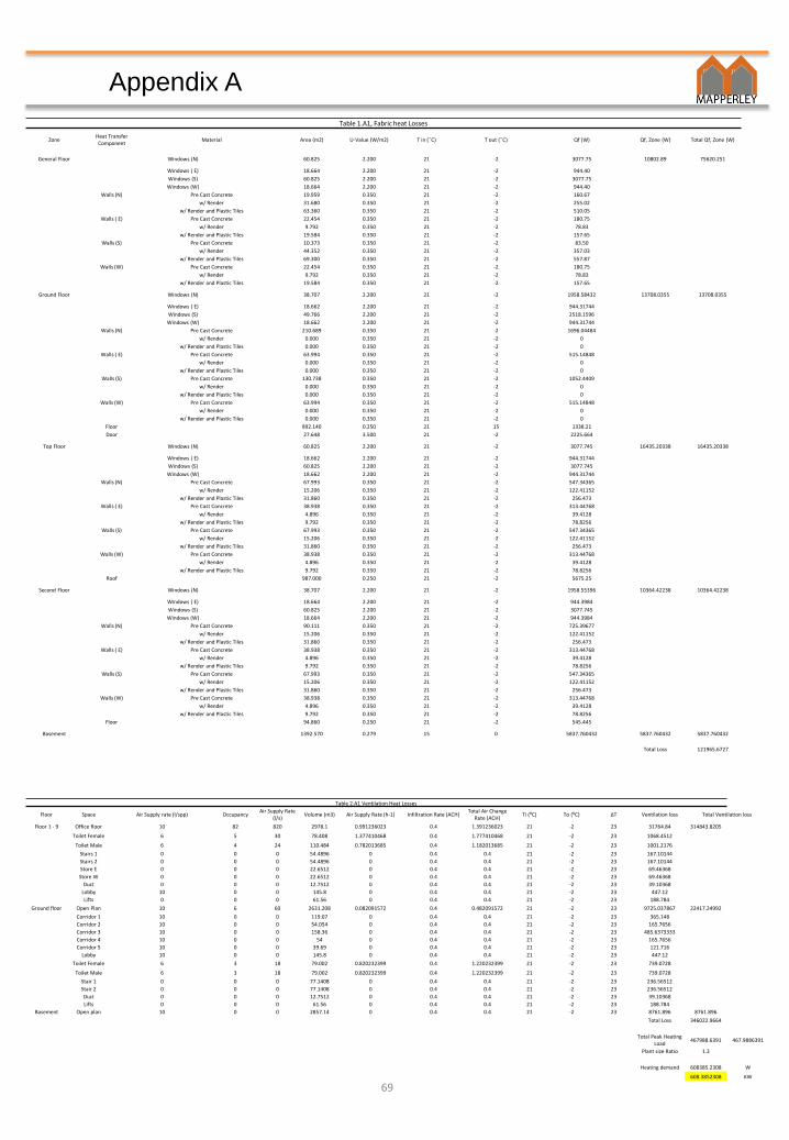
Table 1.A1, Fabric heat Losses
ZoneHeat Transfer Component
Material Area (m2) U-Value (W/m2) T in ( ͦC) T out ( ͦC) Qf (W) Qf, Zone (W) Total Qf, Zone (W)
General Floor Windows (N) 60.825 2.200 21 -2 3077.75 10802.89 75620.251
Windows ( E) 18.664 2.200 21 -2 944.40
Windows (S) 60.825 2.200 21 -2 3077.75
Windows (W) 18.664 2.200 21 -2 944.40
Walls (N) Pre Cast Concrete 19.959 0.350 21 -2 160.67
w/ Render 31.680 0.350 21 -2 255.02
w/ Render and Plastic Tiles 63.360 0.350 21 -2 510.05
Walls ( E) Pre Cast Concrete 22.454 0.350 21 -2 180.75
w/ Render 9.792 0.350 21 -2 78.83
w/ Render and Plastic Tiles 19.584 0.350 21 -2 157.65
Walls (S) Pre Cast Concrete 10.373 0.350 21 -2 83.50
w/ Render 44.352 0.350 21 -2 357.03
w/ Render and Plastic Tiles 69.300 0.350 21 -2 557.87
Walls (W) Pre Cast Concrete 22.454 0.350 21 -2 180.75
w/ Render 9.792 0.350 21 -2 78.83
w/ Render and Plastic Tiles 19.584 0.350 21 -2 157.65
Ground Floor Windows (N) 38.707 2.200 21 -2 1958.58432 13708.0355 13708.0355
Windows ( E) 18.662 2.200 21 -2 944.31744
Windows (S) 49.766 2.200 21 -2 2518.1596
Windows (W) 18.662 2.200 21 -2 944.31744
Walls (N) Pre Cast Concrete 210.689 0.350 21 -2 1696.04484
w/ Render 0.000 0.350 21 -2 0
w/ Render and Plastic Tiles 0.000 0.350 21 -2 0
Walls ( E) Pre Cast Concrete 63.994 0.350 21 -2 515.14848
w/ Render 0.000 0.350 21 -2 0
w/ Render and Plastic Tiles 0.000 0.350 21 -2 0
Walls (S) Pre Cast Concrete 130.738 0.350 21 -2 1052.4409
w/ Render 0.000 0.350 21 -2 0
w/ Render and Plastic Tiles 0.000 0.350 21 -2 0
Walls (W) Pre Cast Concrete 63.994 0.350 21 -2 515.14848
w/ Render 0.000 0.350 21 -2 0
w/ Render and Plastic Tiles 0.000 0.350 21 -2 0
Floor 892.140 0.250 21 15 1338.21
Door 27.648 3.500 21 -2 2225.664
Top Floor Windows (N) 60.825 2.200 21 -2 3077.745 16435.20338 16435.20338
Windows ( E) 18.662 2.200 21 -2 944.31744
Windows (S) 60.825 2.200 21 -2 3077.745
Windows (W) 18.662 2.200 21 -2 944.31744
Walls (N) Pre Cast Concrete 67.993 0.350 21 -2 547.34365
w/ Render 15.206 0.350 21 -2 122.41152
w/ Render and Plastic Tiles 31.860 0.350 21 -2 256.473
Walls ( E) Pre Cast Concrete 38.938 0.350 21 -2 313.44768
w/ Render 4.896 0.350 21 -2 39.4128
w/ Render and Plastic Tiles 9.792 0.350 21 -2 78.8256
Walls (S) Pre Cast Concrete 67.993 0.350 21 -2 547.34365
w/ Render 15.206 0.350 21 -2 122.41152
w/ Render and Plastic Tiles 31.860 0.350 21 -2 256.473
Walls (W) Pre Cast Concrete 38.938 0.350 21 -2 313.44768
w/ Render 4.896 0.350 21 -2 39.4128
w/ Render and Plastic Tiles 9.792 0.350 21 -2 78.8256
Roof 987.000 0.250 21 -2 5675.25
Second Floor Windows (N) 38.707 2.200 21 -2 1958.55396 10364.42238 10364.42238
Windows ( E) 18.664 2.200 21 -2 944.3984
Windows (S) 60.825 2.200 21 -2 3077.745
Windows (W) 18.664 2.200 21 -2 944.3984
Walls (N) Pre Cast Concrete 90.111 0.350 21 -2 725.39677
w/ Render 15.206 0.350 21 -2 122.41152
w/ Render and Plastic Tiles 31.860 0.350 21 -2 256.473
Walls ( E) Pre Cast Concrete 38.938 0.350 21 -2 313.44768
w/ Render 4.896 0.350 21 -2 39.4128
w/ Render and Plastic Tiles 9.792 0.350 21 -2 78.8256
Walls (S) Pre Cast Concrete 67.993 0.350 21 -2 547.34365
w/ Render 15.206 0.350 21 -2 122.41152
w/ Render and Plastic Tiles 31.860 0.350 21 -2 256.473
Walls (W) Pre Cast Concrete 38.938 0.350 21 -2 313.44768
w/ Render 4.896 0.350 21 -2 39.4128
w/ Render and Plastic Tiles 9.792 0.350 21 -2 78.8256
Floor 94.860 0.250 21 -2 545.445
Basement 1392.570 0.279 15 0 5837.760432 5837.760432 5837.760432
Total Loss 121965.6727
Table 2.A1 Ventilation Heat Losses
Floor Space Air Supply rate (l/spp) OccupancyAir Supply Rate
(l/s)Volume (m3) Air Supply Rate (h-1) Infiltration Rate (ACH)
Total Air Change Rate (ACH)
Ti (⁰C) To (⁰C) ΔT Ventilation loss Total Ventilation loss
Floor 1 - 9 Office floor 10 82 820 2978.1 0.991236023 0.4 1.391236023 21 -2 23 31764.84 314843.8205
Toilet Female 6 5 30 78.408 1.377410468 0.4 1.777410468 21 -2 23 1068.4512
Toilet Male 6 4 24 110.484 0.782013685 0.4 1.182013685 21 -2 23 1001.2176
Stairs 1 0 0 0 54.4896 0 0.4 0.4 21 -2 23 167.10144
Stairs 2 0 0 0 54.4896 0 0.4 0.4 21 -2 23 167.10144
Store E 0 0 0 22.6512 0 0.4 0.4 21 -2 23 69.46368
Store W 0 0 0 22.6512 0 0.4 0.4 21 -2 23 69.46368
Duct 0 0 0 12.7512 0 0.4 0.4 21 -2 23 39.10368
Lobby 10 0 0 145.8 0 0.4 0.4 21 -2 23 447.12
Lifts 0 0 0 61.56 0 0.4 0.4 21 -2 23 188.784
Ground floor Open Plan 10 6 60 2631.208 0.082091572 0.4 0.482091572 21 -2 23 9725.037867 22417.24992
Corridor 1 10 0 0 119.07 0 0.4 0.4 21 -2 23 365.148
Corridor 2 10 0 0 54.054 0 0.4 0.4 21 -2 23 165.7656
Corridor 3 10 0 0 158.36 0 0.4 0.4 21 -2 23 485.6373333
Corridor 4 10 0 0 54 0 0.4 0.4 21 -2 23 165.7656
Corridor 5 10 0 0 39.69 0 0.4 0.4 21 -2 23 121.716
Lobby 10 0 0 145.8 0 0.4 0.4 21 -2 23 447.12
Toilet Female 6 3 18 79.002 0.820232399 0.4 1.220232399 21 -2 23 739.0728
Toilet Male 6 3 18 79.002 0.820232399 0.4 1.220232399 21 -2 23 739.0728
Stair 1 0 0 0 77.1408 0 0.4 0.4 21 -2 23 236.56512
Stair 2 0 0 0 77.1408 0 0.4 0.4 21 -2 23 236.56512
Duct 0 0 0 12.7512 0 0.4 0.4 21 -2 23 39.10368
Lifts 0 0 0 61.56 0 0.4 0.4 21 -2 23 188.784
Basement Open plan 10 0 0 2857.14 0 0.4 0.4 21 -2 23 8761.896 8761.896
Total Loss 346022.9664
Total Peak Heating Load
467988.6391 467.9886391
Plant size Ratio 1.3
Heating demand 608385.2308 W
608.3852308 KW

Appendix B
Table 1.B1, Solar Conduction through the glazing
G-Value 0.72
Response Factor
0.8360.5111606
618.3564590
255.4772983
618.3564590
2
May Wall SE Area (m2) G-ValueResponse
FactorSolar Gain SW Area (m2) G-Value
Response Factor
Solar Gain NW Area (m2) G-ValueResponse
FactorSolar Gain NE Area (m2) G-Value
Response Factor
Solar Gain Total Gain
Time
07:30 366 615.1968 0.72 0.83134556.828
4155 186.624 0.72 0.83
17286.60787
128 564.0192 0.72 0.8343143.4078
6370 186.624 0.72 0.83
41264.80589
236251.65
08:30 447 615.1968 0.72 0.83164335.798
6171 186.624 0.72 0.83
19071.03191
143 564.0192 0.72 0.8348199.2759
7302 186.624 0.72 0.83
33681.00372
265287.1102
09:30 493 615.1968 0.72 0.83181247.312
6184 186.624 0.72 0.83
20520.87644
157 564.0192 0.72 0.8352918.0862
1184 186.624 0.72 0.83
20520.87644
275207.1517
10:30 509 615.1968 0.72 0.83187129.578
3196 186.624 0.72 0.83
21859.19447
167 564.0192 0.72 0.8356288.6649
4155 186.624 0.72 0.83
17286.60787
282564.0456
11:30 476 615.1968 0.72 0.83174997.405
3226 186.624 0.72 0.83
25204.98954
174 564.0192 0.72 0.8358648.0700
6165 186.624 0.72 0.83 18401.8729
277252.3378
12:30 404 615.1968 0.72 0.83148527.209
5333 186.624 0.72 0.83 37138.3253 178 564.0192 0.72 0.83
59996.30156
169 186.624 0.72 0.8318847.9789
1264509.815
3
13:30 306 615.1968 0.72 0.83 112498.332 424 186.624 0.72 0.8347287.2370
2177 564.0192 0.72 0.83
59659.24368
168 186.624 0.72 0.83 18736.4524238181.265
1
14:30 205 615.1968 0.72 0.8375366.5295
7487 186.624 0.72 0.83
54313.40667
173 564.0192 0.72 0.8358311.0121
9164 186.624 0.72 0.83
18290.34639
206281.2948
15:30 182 615.1968 0.72 0.83 66910.7726 513 186.624 0.72 0.8357213.0957
3174 564.0192 0.72 0.83
58648.07006
157 186.624 0.72 0.8317509.6608
8200281.599
3
16:30 171 615.1968 0.72 0.8362866.7149
1502 186.624 0.72 0.83 55986.3042 211 564.0192 0.72 0.83 71119.2114 146 186.624 0.72 0.83
16282.86935
206255.0999
17:30 157 615.1968 0.72 0.8357719.7324
1455 186.624 0.72 0.83
50744.55859
325 564.0192 0.72 0.83 109543.809 132 186.624 0.72 0.8314721.4983
2232729.598
3
Table 2.B1, Sol-Air Gains, May
May Render
Area 1229.0318 m2 120.8883738
U-Value 0.35 W/m2/k
t_r 22 °C
t_em 27.47916667 °C
f 0.9
φ 1 hours
SE Sun Time lag time Sol-air temp Qm Q_theta Q_theta+phi
theta (hours) (hours) dark, Teo
1 2 11.3 2356.924525 -4602.724091 -3906.759229
2 3 10.7 2356.924525 -4860.820769 -4139.04624
3 4 9.7 2356.924525 -5290.981899 -4526.191257
4 5 9.3 2356.924525 -5463.046351 -4681.049263
5 6 11.1 2356.924525 -4688.756317 -3984.188233
6 7 25.8 2356.924525 1634.612294 1706.843517
7 8 37.9 2356.924525 6839.561967 6391.298223
8 9 48.5 2356.924525 11399.26995 10495.0354
9 10 54.2 2356.924525 13851.18839 12701.762
10 11 57 2356.924525 15055.63955 13785.76805
11 12 55 2356.924525 14195.31729 13011.47801
12 13 50.4 2356.924525 12216.57609 11230.61094
13 14 42.4 2356.924525 8775.287052 8133.450799
14 15 33 2356.924525 4731.77243 4494.287639
15 16 30.9 2356.924525 3828.434057 3681.283104
16 17 29.3 2356.924525 3140.176249 3061.851077
17 18 26.9 2356.924525 2107.789537 2132.703036
18 19 24.5 2356.924525 1075.402825 1203.554995
19 20 20.9 2356.924525 -473.177243 -190.1670662
20 21 17.4 2356.924525 -1978.741198 -1545.174626
21 22 14.9 2356.924525 -3054.144023 -2513.037168
22 23 13.1 2356.924525 -3828.434057 -3209.898199
23 24 12.9 2356.924525 -3914.466283 -3287.327202
24 25 12.4 2356.924525 -4129.546848 -3480.899711
25 26 11.3 2356.924525 -4602.724091 -3906.759229
26 27 10.7 2356.924525 -4860.820769 -4139.04624
27 28 9.7 2356.924525 -5290.981899 -4526.191257
28 29 9.3 2356.924525 -5463.046351 -4681.049263
29 30 11.1 2356.924525 -4688.756317 -3984.188233
30 31 25.8 2356.924525 1634.612294 1706.843517
31 32 37.9 2356.924525 6839.561967 6391.298223
32 33 48.5 2356.924525 11399.26995 10495.0354
33 34 54.2 2356.924525 13851.18839 12701.762
34 35 57 2356.924525 15055.63955 13785.76805
35 36 55 2356.924525 14195.31729 13011.47801
36 37 50.4 2356.924525 12216.57609 11230.61094
37 38 42.4 2356.924525 8775.287052 8133.450799
38 39 33 2356.924525 4731.77243 4494.287639
39 40 30.9 2356.924525 3828.434057 3681.283104
40 41 29.3 2356.924525 3140.176249 3061.851077
41 42 26.9 2356.924525 2107.789537 2132.703036
42 43 24.5 2356.924525 1075.402825 1203.554995
43 44 20.9 2356.924525 -473.177243 -190.1670662
44 45 17.4 2356.924525 -1978.741198 -1545.174626
45 46 14.9 2356.924525 -3054.144023 -2513.037168
46 47 13.1 2356.924525 -3828.434057 -3209.898199
47 48 12.9 2356.924525 -3914.466283 -3287.327202
48 49 12.4 2356.924525 -4129.546848 -3480.899711
13785.76805
Appendix B
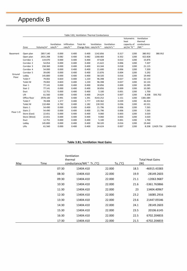
Table 3.B1, Ventilation Thermal Conductance
Zone Volume/mᶟVentilation rate/hˉ¹
Infiltration rate/hˉ¹
Total Air Change Rate
Ventilation rate/mᶟhˉ¹
Ventilation rate/mᶟsˉ¹
Volumetric heat capacity of air/JmˉᶟKˉ¹
Ventilation thermal conductance/WKˉ¹
Basement Open plan 2857.140 0.000 0.400 0.400 1142.856 0.317 1200 380.952 380.952
13404.410
Ground Floor
Open plan 2631.208 0.082 0.400 0.482 1268.483 0.352 1200 422.828
593.702
Corridor 1 119.070 0.000 0.400 0.400 47.628 0.013 1200 15.876
Corridor 2 54.054 0.000 0.400 0.400 21.622 0.006 1200 7.207
Corridor 3 158.360 0.000 0.400 0.400 63.344 0.018 1200 21.115
Corridor 4 54.000 0.000 0.400 0.400 21.600 0.006 1200 7.200
Corridor 5 39.690 0.000 0.400 0.400 15.876 0.004 1200 5.292
Lobby 145.800 0.000 0.400 0.400 58.320 0.016 1200 19.440
Toilet F 79.002 0.820 0.400 1.220 96.398 0.027 1200 32.133
Toilet M 79.002 0.820 0.400 1.220 96.398 0.027 1200 32.133
Stair 1 77.141 0.000 0.400 0.400 30.856 0.009 1200 10.285
Stair 2 77.141 0.000 0.400 0.400 30.856 0.009 1200 10.285
Duct 12.751 0.000 0.400 0.400 5.100 0.001 1200 1.700
Lift 61.560 0.000 0.400 0.400 24.624 0.007 1200 8.208
Floor 1-9
Office floor 2978.100 0.991 0.400 1.391 4143.252 1.151 1200 1381.084
12429.756
Toilet F 78.408 1.377 0.400 1.777 139.362 0.039 1200 46.454
Toilet M 110.484 0.782 0.400 1.182 130.592 0.036 1200 43.531
Stairs 1 54.490 0.000 0.400 0.400 21.796 0.006 1200 7.265
Stairs 2 54.490 0.000 0.400 0.400 21.796 0.006 1200 7.265
Store (East) 22.651 0.000 0.400 0.400 9.060 0.003 1200 3.020
Store (West) 22.651 0.000 0.400 0.400 9.060 0.003 1200 3.020
Duct 12.751 0.000 0.400 0.400 5.100 0.001 1200 1.700
Lobby 145.800 0.000 0.400 0.400 58.320 0.016 1200 19.440
Lifts 61.560 0.000 0.400 0.400 24.624 0.007 1200 8.208
Table 3.B1, Ventilation Heat Gains
May Time
Ventilation thermal conductance/WKˉ¹ Tr, (°C) To, (°C)
Total Heat Gains (W)
07:30 13404.410 22.000 18.5 -46915.43383
08:30 13404.410 22.000 19.9 -28149.2603
09:30 13404.410 22.000 21.1 -12063.9687
10:30 13404.410 22.000 21.6 -5361.763866
11:30 13404.410 22.000 23 13404.40967
12:30 13404.410 22.000 23.2 16085.2916
13:30 13404.410 22.000 23.6 21447.05546
14:30 13404.410 22.000 24.1 28149.2603
15:30 13404.410 22.000 23.5 20106.6145
16:30 13404.410 22.000 22.5 6702.204833
17:30 13404.410 22.000 21.5 -6702.204833

Appendix B
.
72
Table 5.B1Roof Sol-air Temperatures
Roof
Area 987 m2
U-Value 0.54 W/m2/k
t_r 22 °C
t_em 26.2 °C
f 0.17
φ 9 hours
May
Sun Time Ѳ (h) lag Time ф (h)Sol-air temp
Dark TeoQm Q_Ѳ Q_Ѳ+ф
1 10 9.6 2238.516 -6608.952 734.44644
2 11 9 2238.516 -6928.74 680.08248
3 12 7.7 2238.516 -7621.614 562.2939
4 13 7.3 2238.516 -7834.806 526.05126
5 14 9.7 2238.516 -6555.654 743.5071
6 15 15.2 2238.516 -3624.264 1241.8434
7 16 23.2 2238.516 639.576 1966.6962
8 17 31.8 2238.516 5223.204 2745.91296
9 18 38.2 2238.516 8634.276 3325.7952
10 19 44 2238.516 11725.56 3851.31348
11 20 47.6 2238.516 13644.288 4177.49724
12 21 50.3 2238.516 15083.334 4422.13506
13 22 50.4 2238.516 15136.632 4431.19572
14 23 49.3 2238.516 14550.354 4331.52846
15 24 46.7 2238.516 13164.606 4095.9513
16 25 41.9 2238.516 10606.302 3661.03962
17 26 35.9 2238.516 7408.422 3117.40002
18 27 29.9 2238.516 4210.542 2573.76042
19 28 21.5 2238.516 -266.49 1812.66498
20 29 15.8 2238.516 -3304.476 1296.20736
21 30 12.9 2238.516 -4850.118 1033.44822
22 31 10.9 2238.516 -5916.078 852.23502
23 32 10.7 2238.516 -6022.674 834.1137
24 33 10.4 2238.516 -6182.568 806.93172
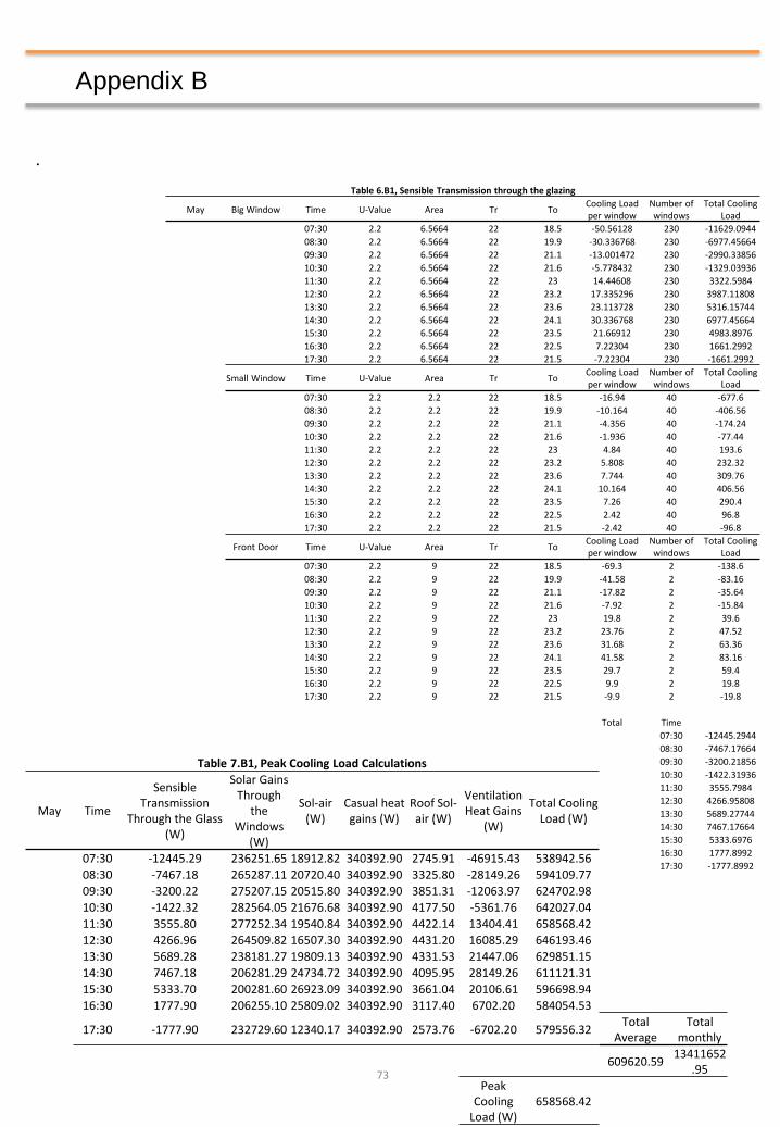
Appendix B
.
73
Table 7.B1, Peak Cooling Load Calculations
May Time
Sensible Transmission
Through the Glass (W)
Solar Gains Through
the Windows
(W)
Sol-air (W)
Casual heat gains (W)
Roof Sol-air (W)
Ventilation Heat Gains
(W)
Total Cooling Load (W)
07:30 -12445.29 236251.65 18912.82 340392.90 2745.91 -46915.43 538942.56
08:30 -7467.18 265287.11 20720.40 340392.90 3325.80 -28149.26 594109.77
09:30 -3200.22 275207.15 20515.80 340392.90 3851.31 -12063.97 624702.98
10:30 -1422.32 282564.05 21676.68 340392.90 4177.50 -5361.76 642027.04
11:30 3555.80 277252.34 19540.84 340392.90 4422.14 13404.41 658568.42
12:30 4266.96 264509.82 16507.30 340392.90 4431.20 16085.29 646193.46
13:30 5689.28 238181.27 19809.13 340392.90 4331.53 21447.06 629851.15
14:30 7467.18 206281.29 24734.72 340392.90 4095.95 28149.26 611121.31
15:30 5333.70 200281.60 26923.09 340392.90 3661.04 20106.61 596698.94
16:30 1777.90 206255.10 25809.02 340392.90 3117.40 6702.20 584054.53
17:30 -1777.90 232729.60 12340.17 340392.90 2573.76 -6702.20 579556.32Total
AverageTotal
monthly
609620.5913411652
.95
Peak Cooling
Load (W)658568.42
Table 6.B1, Sensible Transmission through the glazing
May Big Window Time U-Value Area Tr ToCooling Load per window
Number of windows
Total Cooling Load
07:30 2.2 6.5664 22 18.5 -50.56128 230 -11629.0944
08:30 2.2 6.5664 22 19.9 -30.336768 230 -6977.45664
09:30 2.2 6.5664 22 21.1 -13.001472 230 -2990.33856
10:30 2.2 6.5664 22 21.6 -5.778432 230 -1329.03936
11:30 2.2 6.5664 22 23 14.44608 230 3322.5984
12:30 2.2 6.5664 22 23.2 17.335296 230 3987.11808
13:30 2.2 6.5664 22 23.6 23.113728 230 5316.15744
14:30 2.2 6.5664 22 24.1 30.336768 230 6977.45664
15:30 2.2 6.5664 22 23.5 21.66912 230 4983.8976
16:30 2.2 6.5664 22 22.5 7.22304 230 1661.2992
17:30 2.2 6.5664 22 21.5 -7.22304 230 -1661.2992
Small Window Time U-Value Area Tr ToCooling Load per window
Number of windows
Total Cooling Load
07:30 2.2 2.2 22 18.5 -16.94 40 -677.6
08:30 2.2 2.2 22 19.9 -10.164 40 -406.56
09:30 2.2 2.2 22 21.1 -4.356 40 -174.24
10:30 2.2 2.2 22 21.6 -1.936 40 -77.44
11:30 2.2 2.2 22 23 4.84 40 193.6
12:30 2.2 2.2 22 23.2 5.808 40 232.32
13:30 2.2 2.2 22 23.6 7.744 40 309.76
14:30 2.2 2.2 22 24.1 10.164 40 406.56
15:30 2.2 2.2 22 23.5 7.26 40 290.4
16:30 2.2 2.2 22 22.5 2.42 40 96.8
17:30 2.2 2.2 22 21.5 -2.42 40 -96.8
Front Door Time U-Value Area Tr ToCooling Load per window
Number of windows
Total Cooling Load
07:30 2.2 9 22 18.5 -69.3 2 -138.6
08:30 2.2 9 22 19.9 -41.58 2 -83.16
09:30 2.2 9 22 21.1 -17.82 2 -35.64
10:30 2.2 9 22 21.6 -7.92 2 -15.84
11:30 2.2 9 22 23 19.8 2 39.6
12:30 2.2 9 22 23.2 23.76 2 47.52
13:30 2.2 9 22 23.6 31.68 2 63.36
14:30 2.2 9 22 24.1 41.58 2 83.16
15:30 2.2 9 22 23.5 29.7 2 59.4
16:30 2.2 9 22 22.5 9.9 2 19.8
17:30 2.2 9 22 21.5 -9.9 2 -19.8
Total Time
07:30 -12445.2944
08:30 -7467.17664
09:30 -3200.21856
10:30 -1422.31936
11:30 3555.7984
12:30 4266.95808
13:30 5689.27744
14:30 7467.17664
15:30 5333.6976
16:30 1777.8992
17:30 -1777.8992
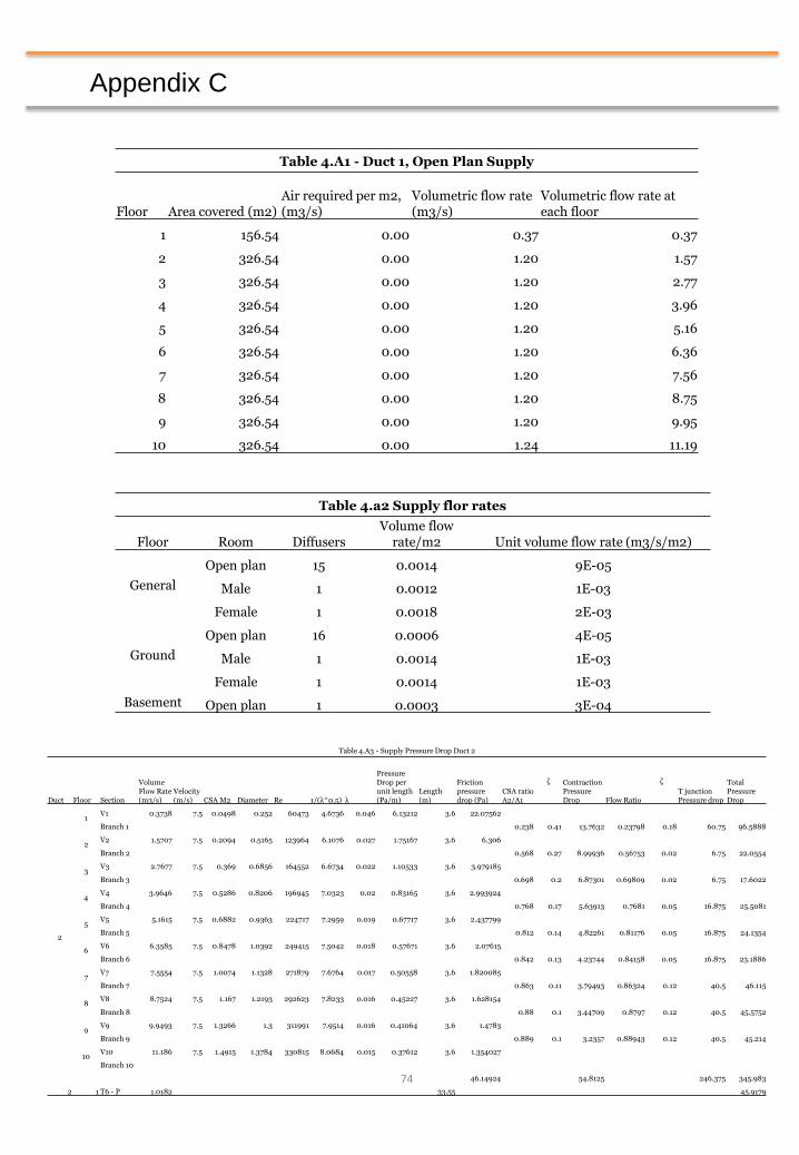
Appendix C
74
Table 4.A1 - Duct 1, Open Plan Supply
Floor Area covered (m2)Air required per m2, (m3/s)
Volumetric flow rate (m3/s)
Volumetric flow rate at each floor
1 156.54 0.00 0.37 0.37
2 326.54 0.00 1.20 1.57
3 326.54 0.00 1.20 2.77
4 326.54 0.00 1.20 3.96
5 326.54 0.00 1.20 5.16
6 326.54 0.00 1.20 6.36
7 326.54 0.00 1.20 7.56
8 326.54 0.00 1.20 8.75
9 326.54 0.00 1.20 9.95
10 326.54 0.00 1.24 11.19
Table 4.a2 Supply flor rates
Floor Room DiffusersVolume flow
rate/m2 Unit volume flow rate (m3/s/m2)
General
Open plan 15 0.0014 9E-05
Male 1 0.0012 1E-03
Female 1 0.0018 2E-03
Ground
Open plan 16 0.0006 4E-05
Male 1 0.0014 1E-03
Female 1 0.0014 1E-03
Basement Open plan 1 0.0003 3E-04
Table 4.A3 - Supply Pressure Drop Duct 2
Duct Floor Section
Volume Flow Rate (m3/s)
Velocity (m/s) CSA M2 Diameter Re 1/(λ^0.5) λ
Pressure Drop per unit length (Pa/m)
Length (m)
Friction pressure drop (Pa)
CSA ratio A2/A1
ζ Contraction Pressure Drop Flow Ratio
ζ
T junction Pressure drop
Total Pressure Drop
2
1V1 0.3738 7.5 0.0498 0.252 60473 4.6736 0.046 6.13212 3.6 22.07562
Branch 1 0.238 0.41 13.7632 0.23798 0.18 60.75 96.5888
2V2 1.5707 7.5 0.2094 0.5165 123964 6.1076 0.027 1.75167 3.6 6.306
Branch 2 0.568 0.27 8.99936 0.56753 0.02 6.75 22.0554
3V3 2.7677 7.5 0.369 0.6856 164552 6.6734 0.022 1.10533 3.6 3.979185
Branch 3 0.698 0.2 6.87301 0.69809 0.02 6.75 17.6022
4V4 3.9646 7.5 0.5286 0.8206 196945 7.0323 0.02 0.83165 3.6 2.993924
Branch 4 0.768 0.17 5.63913 0.7681 0.05 16.875 25.5081
5V5 5.1615 7.5 0.6882 0.9363 224717 7.2959 0.019 0.67717 3.6 2.437799
Branch 5 0.812 0.14 4.82261 0.81176 0.05 16.875 24.1354
6V6 6.3585 7.5 0.8478 1.0392 249415 7.5042 0.018 0.57671 3.6 2.07615
Branch 6 0.842 0.13 4.23744 0.84158 0.05 16.875 23.1886
7V7 7.5554 7.5 1.0074 1.1328 271879 7.6764 0.017 0.50558 3.6 1.820085
Branch 7 0.863 0.11 3.79493 0.86324 0.12 40.5 46.115
8V8 8.7524 7.5 1.167 1.2193 292623 7.8233 0.016 0.45227 3.6 1.628154
Branch 8 0.88 0.1 3.44709 0.8797 0.12 40.5 45.5752
9V9 9.9493 7.5 1.3266 1.3 311991 7.9514 0.016 0.41064 3.6 1.4783
Branch 9 0.889 0.1 3.2357 0.88943 0.12 40.5 45.214
10V10 11.186 7.5 1.4915 1.3784 330815 8.0684 0.015 0.37612 3.6 1.354027
Branch 10
46.14924 54.8125 246.375 345.983
2 1 T6 - P 1.0182 33.55 45.9179

Appendix C
75
Table 4.a4 Extract Pressure Drop
Duct Floor SectionVolume Flow Rate (m3/s) Velocity
(m/s)
CSA M2 Diameter Re 1/(λ^0.5) λPressure Drop per
unit length (Pa/m)
Length (m)Friction
pressure drop (Pa)
CSA ratio A2/A1
ζContraction
Pressure DropFlow Ratio ζ
T junction Pressure drop
Total Pressure
Drop
1
1 V1 0.386680301 7.5 0.051557 0.256278 61506.61 4.707489 0.045125 5.94271107 3.6 21.39375985
Branch 1 0.222242 0.414098 13.97581943 0.222242 0.18 6.075 41.44458
2 V2 1.739909007 7.5 0.231988 0.543623 130469.5 6.209737 0.025933 1.610013825 3.6 5.796049769 0
Branch 2 0.562506 0.268967 9.077635513 0.562506 0.02 0.675 15.54869
3 V3 3.093137714 7.5 0.412418 0.724827 173958.4 6.784418 0.021726 1.011612999 3.6 3.641806796 0
Branch 3 0.695655 0.204878 6.914618852 0.695655 0.02 0.675 11.23143
4 V4 4.446366421 7.5 0.592849 0.869035 208568.4 7.146894 0.019578 0.760329652 3.6 2.737186748 0
Branch 4 0.766668 0.167861 5.66531322 0.766668 0.05 1.6875 10.09
5 V5 5.799595127 7.5 0.773279 0.992507 238201.6 7.412283 0.018201 0.618922749 3.6 2.228121895 0
Branch 5 0.810812 0.14343 4.840765406 0.810812 0.05 1.6875 8.756387
6 V6 7.152823834 7.5 0.95371 1.102233 264535.9 7.621755 0.017214 0.527096956 3.6 1.89754904 0
Branch 6 0.84091 0.125951 4.250853495 0.84091 0.05 1.6875 7.835903
7 V7 8.506052541 7.5 1.13414 1.201984 288476.1 7.794821 0.016458 0.462128621 3.6 1.663663036 0
Branch 7 0.862746 0.112749 3.80529422 0.862746 0.12 4.05 9.518957
8 V8 9.859281247 7.5 1.314571 1.294068 310576.4 7.942282 0.015853 0.41345282 3.6 1.48843015 0
Branch 8 0.879311 0.102381 3.455373927 0.879311 0.12 4.05 8.993804
9 V9 11.21250995 7.5 1.495001 1.380022 331205.2 8.070747 0.015352 0.375457103 3.6 1.351645571 0
Branch 9 0.889116 0.096077 3.242612379 0.889116 0.12 4.05 8.644258
10 V10 12.61084965 7.5 1.681447 1.463547 351251.3 8.188136 0.014915 0.343951346 3.6 1.238224845
Branch 10
43.4364377 55.22828644 24.6375 122.064 147.3355
1 T1 - I 0.986932968 0 25.27153

CV’s
.
76

CV’s
.
77
CV’s
.
78

CV’s
.
79

CV’s
.
80
CV’s
.
81

CV’s
.
82

CV’s
.
83

CV’s
.
84