& aer journal of aeronautics & aerospace engineering · citation: minami y (2015) space...

Volume 4 • Issue 2 • 1000149J Aeronaut Aerospace EngISSN: 2168-9792 JAAE, an open access journal

Open AccessResearch Article

Minami, J Aeronaut Aerospace Eng 2015, 4:2 DOI: 10.4172/2168-9792.1000149

Keywords: Space-time; Continuum; Space drive; Propulsion;Curvature; Vacuum; Cosmology; Inflation; Imaginary time; Interstellar travel; Hyper-space; Wormhole; Time-hole

IntroductionA distant galaxy exploration is the dream of mankind. However as

is well known, galaxy travel and interstellar travel are impossible for the present propulsion theory by rocket. The reason is due to the low speed of rocket based on momentum thrust.

At the present stage of space propulsion technology, the only practical propulsion system is chemical propulsion system and electric propulsion system, which are based on expulsion of a mass to induce a momentum thrust. Since the maximum speed is limited by the product of the gas effective exhaust velocity and the natural logarithm of mass ratio, its speed is too slow for the spaceship to achieve the interplanetary travel and interstellar travel. Thus the breakthrough of propulsion method has been required until now. Instead of conventional chemical propulsion systems, field propulsion systems, which are based on General Relativity Theory, Quantum Field Theory and other exotic theories, have been proposed by many researchers to overcome the speed limit of the conventional space rocket. Field propulsion system is the concept of propulsion theory of spaceship not based on usual momentum thrust but based on pressure thrust derived from an interaction of the spaceship with external fields. Field propulsion system is propelled without mass expulsion. The propulsive force is a pressure thrust which arises from the interaction of space-time around the spaceship and the spaceship itself; the spaceship is propelled against space-time structure.

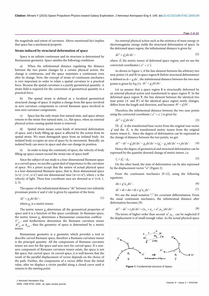
On the other hand, interstellar travel or galaxy travel, i.e., the method that the human arrives at extrasolar planet like super-Earth as the second earth becomes feasible by the combination of space propulsion technology (which accelerates spaceship to the quasi-light velocity in a short time) and navigation technology used wormhole or time hole (which circumvents a wall of the velocity of light). They are space drive propulsion system and Hyper-Space navigation system. Space drive propulsion system is one of the field propulsion system utilizing the action of the medium of strained or deformed field of

space. The curvature of space plays a significant role for the propulsion theory. In the first place, the elucidation of structure of the physical property of the space as vacuum becomes basic. We also should know that any propulsion system cannot exceed the light velocity as characteristic of space, that is to say, there is no propulsion theory which exceeds the velocity of light.

Based on the supposition that space is an infinite continuum like elastic body, space drive propulsion principle induced by spatial curvature and hyper-space navigation theory using imaginary time are introduced in this paper. By the combined use of these both propulsion theory and navigation theory, a realistic interstellar exploration can be possible.

Like the Wright brothers who succeeded in a human first power flight in 1903; they elucidated a property of the air by the flow of invisible transparent air using a wind tunnel experiment, mankind must study the property and fine structure of space in earnest

In the near future, the next target of mankind who completed solar system exploration will go to stellar system or galaxy exploration. Moreover, although the SETI project planned in each country until now is premised on actual existence of extraterrestrial intelligent life, the contact with them is made impossible by lack of the navigation theory and propulsion technology which can conquer a huge distance between stars and Earth. That is, even if the speed of light is obtained, we have to spend the very long hours underway which will be required

*Corresponding author: Yoshinari Minami, Advanced Science-TechnologyResearch Organization (Formerly NEC Space Development Division), 35-13,Higashikubo-Cho, Nishi-Ku, Yokohama, 220-0062 Japan, Tel: 022-277-6611,E-mail: [email protected]

Received November 04, 2015; Accepted November 21, 2015; Published November 28, 2015

Citation: Minami Y (2015) Space Propulsion Physics toward Galaxy Exploration. J Aeronaut Aerospace Eng 4: 149. doi:10.4172/2168-9792.1000149

Copyright: © 2015 Minami Y. This is an open-access article distributed underthe terms of the Creative Commons Attribution License, which permits unrestricted use, distribution, and reproduction in any medium, provided the original author and source are credited.

AbstractThe distance to a stellar system is too huge, therefore the travel to the fixed star nearest to the Earth using

the present propulsion technology will require tens of thousands years. In order to overcome such a limit of the space travel between fixed stars, research and development of a new propulsion theory and navigation theory are indispensable. As a promising approach, space drive propulsion theory and Hyper-Space navigation method given by a space-time featuring an imaginary time (i.e., Time-Hole) are introduced.

Space drive propulsion system is one of field propulsion system utilizing the action of the medium of strained or deformed field of space. The curvature of space plays a significant role for the propulsion theory. On the other hand, a plunging into Hyper-Space characterized by imaginary time would make the interstellar travel possible in a short time. The Hyper-Space navigation theory would allow a starship to start at any time and from any place for an interstellar travel to the farthest star systems, the whole mission time being within human lifetime.

Space propulsion physics such as propulsion theory and navigation theory give us a concrete theoretical method toward galaxy exploration. This paper describes a summary of each theme (Continuum mechanics of Space-Time, Space drive propulsion, Hyper-Space navigation) published so far by author.

Space Propulsion Physics toward Galaxy ExplorationYoshinari Minami* Advanced Science-Technology Research Organization (Formerly NEC Space Development Division), Japan

Journal of Aeronautics & Aerospace EngineeringJo

urna

l of A

eron

autics & Aerospace Engineering

ISSN: 2168-9792


of 20


As a conclusion, the practical interstellar travel combines propulsion theory with navigation theory.

The term of “Space Propulsion Physics” indicates both propulsion theory and navigation theory using the physical property of space-time.

In the subsequent chapters, mechanical structure of space-time in the first, space drive propulsion in the second, and finally Hyper-Space navigation using “Imaginary Time-Hole” are introduced.

Continuum Mechanics of Space-timeGiven a priori assumption that space as a vacuum has a physical fine

structure like continuum, it enables us to apply a continuum mechanics to the so-called “vacuum” of space. Minami investigated a hypothesis for mechanical property of space-time in 1986 [1]. A primary motive was research in the realm of space propulsion theory. His propulsion principle using the substantial physical structure of space-time based on this hypothesis was proposed in 1988 [2].

In this chapter, a fundamental concept of space-time is described that focuses on theoretically innate properties of space including strain and curvature.

Assuming that space as vacuum is an infinite continuum, space can be considered as a kind of transparent elastic field. That is, space as a vacuum performs the motions of deformation such as expansion, contraction, elongation, torsion and bending. The latest expanding universe theories (Friedmann, de Sitter, inflationary cosmological model) support this assumption. Space can be regarded as an elastic body like rubber. This conveniently coincides with the precondition of a mechanical structure of space.

General relativity implies that space is curved by the existence of energy (mass energy or electromagnetic energy etc.). General relativity is based on Riemannian geometry. If we admit this space curvature, space is assumed as an elastic body. According to continuum mechanics, the elastic body has the property of the motion of deformation such as expansion, contraction, elongation, torsion and bending. General relativity uses only the curvature of space. Expansion and contraction of space are used in cosmology. Further, a theory using torsion studied by Hayasaka [7] and twistor theory proposed by Roger Penrose [8] are also applied to the torsion of space.

Acceleration of gravity at the surface of the earth

Let’s think about gravity. When we make a comparison between the space on the Earth and outer space throughout the universe, although there seems to be no difference, obviously a different phenomenon occurs. Simply put, an object moves radially inward, that is, drops straight down on the Earth, but in the universe, the object floats and does not move.

The difference between the two phenomena can be explained as whether space is curved or not, that is, whether 20 independent components of a Riemann curvature tensor is zero or not. In essence, the existence of spatial curvature (curved extent region) determines whether the object drops straight down or not. Although the spatial curvature at the surface of the Earth is very small value, i.e., 23 23.42 10 (1/ )m−× , it is of enough value to produce 1G(9.8m/s2) acceleration. Conversely, the spatial curvature in the universe is zero; therefore any acceleration is not produced. Accordingly, if the spatial curvature of a localized area including object is controlled to curvature

23 23.42 10 (1/ )m−× with an extent, the object moves and receives 1G acceleration in the universe. Of course, we are required to control both

for tens of several years to hundreds years.

Considerable years are required even if it carries out an interstellar travel or galaxy travel with the speed of light.

In order to conquer this huge distance and time, it is said to be that superluminal velocity becomes indispensable. Then, although the superluminal velocity tends to be expected simplistically, it becomes unreal expectation regrettably from the basic theory on physics and restrictions of the propulsion theory. It is because there exists the wall of the velocity of light by Special Relativity, any propulsion principle cannot exceed the velocity of light, and there is no energy source as the power source accelerated to that the wall of the velocity of light. The Special Relativity theory acts correctly in the actual space and any propulsion theory cannot exceed the wall of the velocity of light.

Not only propulsion theory but also a new navigation theory becomes indispensable for the stellar system exploration or galaxy exploration as which the cruising range of a light-year unit is required.

Although the navigation by the Special Relativity is well known as this kind of a navigation theory, it is the unreal navigation which does not become useful due to the extreme time gap of global time and spaceship time (twin or time paradox). Even if we could reach to the fixed star in several years, what 100 years and what 1000 years had passed when it returned to the Earth of the hometown. It becomes a space travel of a one-way ticket literally.

Therefore, the research of the space warp which uses the wormhole by General Relativity and the Hyper-Space navigation theory with the character of imaginary time are required to remove the extreme time gap (between spaceship time and Earth time). Regrettably, since the size of wormhole (i.e., ~10-35m) is smaller than the atom (i.e., ~10-10m) and moreover the size is predicted to fluctuate theoretically due to instabilities, space flight through the wormhole is difficul technically, and it is unknown where to go and how to return. Additionally, since the solution of wormhole includes a singularity, this navigation method theoretically includes fundamental problems. Furthermore, though it is often pointed out, we cannot simply capture and enlarge a quantum size of wormhole. Whatever energy is required to keep the throat open? That is, wormhole requires exotic energy to enlarge the throat enough for passage of a starship through the wormhole. It is not feasible as an idea.

Minami completed the things that had been investigated about mechanics of space in 1986 [1].

A primary motive was research in the realm of space propulsion theory. His propulsion principle is based on the substantial physical structure of space-time. After then, a concept of a space drive propulsion system as a paper entitled “Space Strain Propulsion System” was introduced by Minami in 1988 [2]. The term of “space strain” was changed to “space drive” receiving the recommendation by Forward [3]. After then, the second paper entitled “Possibility of Space Drive Propulsion” was presented at the 45th IAF in 1994 [4].

At the same time, Minami proposed the Hyper-Space navigation theory used imaginary time in 1993 [5]. A plunging into Hyper-Space characterized by imaginary time would make the interstellar travel possible in a short time. The Hyper-Space navigation theory would allow a starship to start at any time and from any place for an interstellar travel to the farthest star systems, the whole mission time being within human lifetime [6]. This proposed navigation theory is based on Special Relativity (not on General Relativity).


of 20


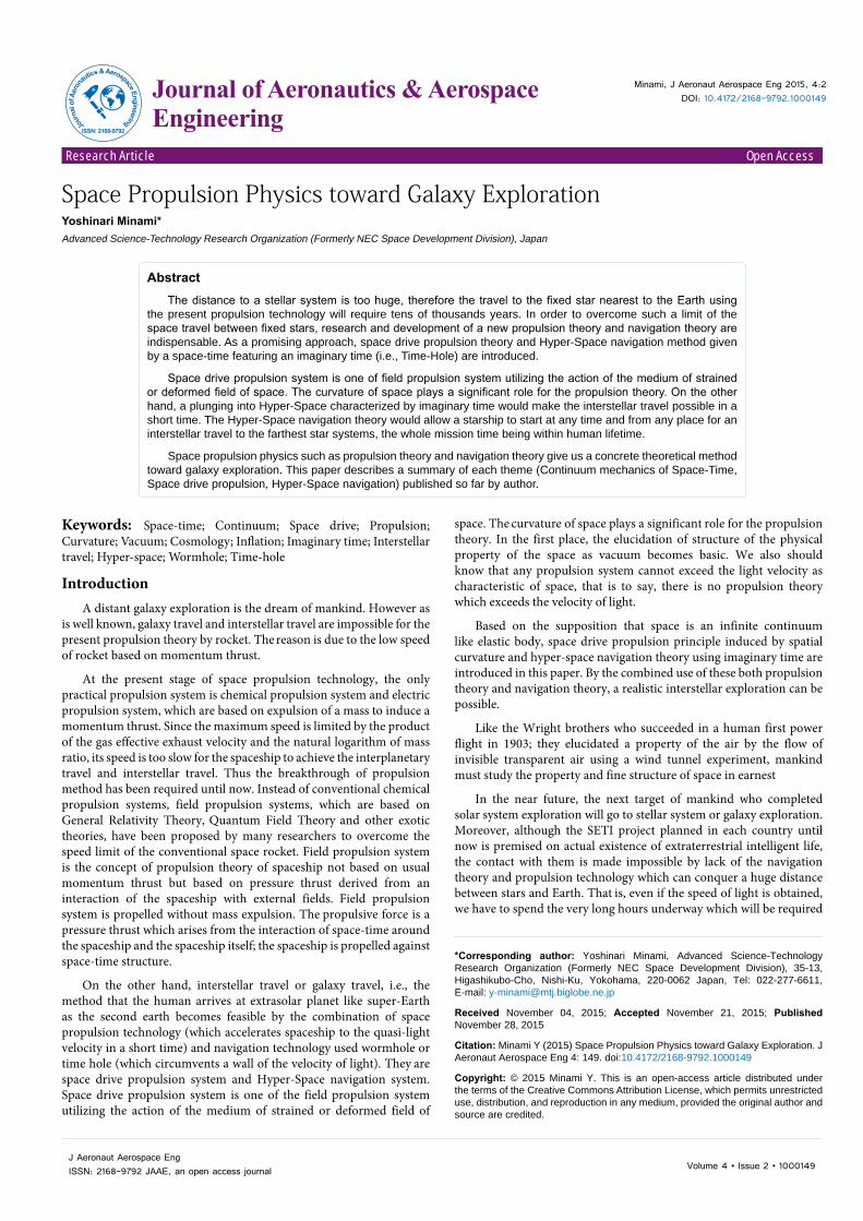
An external physical action such as the existence of mass energy or electromagnetic energy yields the structural deformation of space. In the deformed space region, the infinitesimal distance is given by:

2 i jijds g dx dx′ ′= , (2)

where ijg ′ the metric tensor of deformed space region, and we use the convected coordinates ( i ix x′ = ).

As shown in Figure 1, if the line element between the arbitrary two near points (A and B) in space region S (before structural deformation) is defined as i

ids g dx= , the infinitesimal distance between the two near points is given by Eq.(1): 2 i j

ijds g dx dx= .

Let us assume that a space region S is structurally deformed by an external physical action and transformed to space region T. In the deformed space region T, the line element between the identical two near point (A’ and B’) of the identical space region newly changes, differs from the length and direction, and becomes i

ids g dx′ ′= .

Therefore, the infinitesimal distance between the two near points using the convected coordinate ( i ix x′ = ) is given by:

2 i jijds g dx dx′ ′= . (3)

Th ig ′ is the transformed base vector from the original vase vector ig and the ijg ′ is the transformed metric tensor from the original

metric tensor ijg . Since the degree of deformation can be expressed as the change of distance between the two points, we get:

2 2 ( )i j i j i j i jij ij ij ij ijds ds g dx dx g dx dx g g dx dx r dx dx′ ′ ′− = − = − = . (4)

Hence the degree of geometrical and structural deformation can be expressed by the quantity denoted change of metric tensor, i.e.

ij ij ijr g g′= − . (5)

On the other hand, the state of deformation can be also expressed by the displacement vector “u” (Figure 2).

From the continuum mechanics [9-12], using the following equations:

:i j

i jdu g u dx= , (6)

:i j

i jds ds du ds g u dx′ = + = + . (7)

We use the usual notation “:” for covariant differentiation. From the usual continuum mechanics, the infinitesimal distance afterdeformation becomes [9]:

2 2: : : :( )i j k i j

ij i j j i i k jds ds r dx dx u u u u dx dx′ − = = + + . (8)

The terms of higher order than second : :k

i k ju u can be neglected if the displacement is of small enough value. As the actual physical space

the magnitude and extent of curvature. Above-mentioned fact implies that space has a mechanical property.

Strain induced by structural deformation of space

Space is an infinite continuum and its structure is determined by Riemannian geometry. Space satisfies the following conditions

a) When the infinitesimal distance regulating the distance between the two points changes by a certain physical action, the change is continuous, and the space maintains a continuum even after its change. Now, the concept of strain of continuum mechanics is very important in order to relate a spatial curvature to a practical force. Because the spatial curvature is a purely geometrical quantity. A strain field is required for the conversion of geometrical quantity to a practical force.

b) The spatial strain is defined as a localized geometrical structural change of space. It implies a change from flat space involved in zero curvature components to curved Riemann space involved in non-zero curvature components.

c) Space has the only strain-free natural state, and space always returns to the strain-free natural state, i.e., flat space, when an external physical action causing spatial strain is removed.

d) Spatial strain means some kinds of structural deformation of space, and a body filling up space is affected by the action from its spatial strain. We must distinguish space from an isolated body. An isolated body occupies an area of space by its movement. Basically, an isolated body can move in space and also can change its position.

e) In order to keep the continuity of space, the velocity of body filling up space cannot exceed the strain rate of space itself

Since the subject of our study is a four-dimensional Riemann space as a curved space, we ascribe a great deal of importance to the curvature of space. We a priori accept that the nature of actual physical space is a four-dimensional Riemann space, that is, three dimensional space (x=x1, y=x2, z=x3) and one dimensional time (w=ct=x0), where c is the velocity of light. These four coordinate axes are denoted as xi (i=0, 1, 2, 3).

The square of the infinitesimal distance “ds” between two infinitelyproximate points xi and xi+dxi is given by equation of the form:

2 i jijds g dx dx= , (1)

where gij is a metric tensor.

The metric tensor gij determines all the geometrical properties of space and it is a function of this space coordinate. In Riemann space, the metric tensor gij determines a Riemannian connection coefficie

ijkΓ , and furthermore determines the Riemann curvature tensor

pijk pijkR or R , thus the geometry of space is determined by a metric

tensor.

Riemannian geometry is a geometry which provides a tool to describe curved Riemann space, therefore a Riemann curvature tensor is the principal quantity. All the components of Riemann curvature tensor are zero for flat space and non-zero for curved space. If a non-zero component of Riemann curvature tensor exists, the space is not flat space, but curved space. In curved space, it is well known that the result of the parallel displacement of vector depends on the choice of the path. Further, the components of a vector differ from the initial value, after we displace a vector parallel along a closed curve until it returns to the starting point.

Figure 1: Fundamental structure of Space.


of 20


can be dealt with the minute displacement from the trial calculation of strain, we get:

: :ij i j j ir u u= + . (9)

Whereas, according to the continuum mechanics [9], the strain tensor ije is given by:

: :1 1 ( )2 2ij ij i j j ie r u u= ⋅ = ⋅ + . (10)

So, we get:2 2 ( ) 2i j i j

ij ij ijds ds g g dx dx e dx dx′ ′− = − = , (11)

where ,ij ijg g′ is a metric tensor, ije is a strain tensor, and 2 2ds ds′ − is the

square of the infinitesimal distance between two infinitely proximate points xi and xi+dxi.

Eq.(11) indicates that a certain geometrical structural deformation of space is shown by the concept of strain. In essence, the change of metric tensor ( )ij ijg g′ − due to the existence of mass energy or electromagnetic energy tensor produces the strain fiel ije .

Since space-time is distorted, the infinitesimal distance between two infinitely proximate points xi and xi+dxi is important in our understanding of the geometry of the space-time; the physical strain is generated by the difference of a geometrical metric of space-time. Namely, a certain structural deformation is described by strain tensor

ije . From Eq.(11), the strain of space is described as follows:

1/ 2 ( ' )ij ij ije g g= ⋅ − . (12)

It is also worth noting that this result yields the principle of constancy of light velocity in Special Relativity.

Body force and rotation of displacement field in curved space

Expanding the concept of vector parallel displacement in Riemann space, the following equation has newly been obtained:

klklR dAµν µνω = , (13)

where µνω is rotation tensor, kldA is infinitesimal areal element.

According to the nature of Riemann curvature tensor klRµν , µνωindicates the rotation of displacement field. Eq.(13) indicates that a curved space produces the rotation of displacement field in the region of space. Now, the rotation tensor µνω and strain tensor ije satisfy the following differential equation in continuum mechanics

, , ,j j je eµν ν µ µ νω = − . (14)

This equation is true on condition that the order of differentialcan be exchanged in a flat space. To expand above equation into a curved Riemann space, the equation shall be transformed to covariant differentiation and it is possible on condition of j je eα α

ν µα µ ναΓ = Γ .

Thus, we obtai

: : :j j je eµν ν µ µ νω = − . (15)

Here we use the usual notation “:” for covariant differentiation

As is well known, the partial derivative ,i

i j j

uu

x∂

=∂

is not tensor

equation. The covariant derivative : ,k

i j i j k iju u u= − Γ is tensor equation and can be carried over into all coordinate systems.

Eq.(15) indicates that the displacement gradient of rotation tensor corresponds to difference of the displacement gradient of strain tensor.

Here, if we multiply both sides of Eq.(15) by fourth order tensor denoted the nature of space ijE µν formally, we obtain

: : :( )ij ij kl ij klj kl j kl jE E R dA E R dAµν µν µν

µν µν µνω = = , (16)

and

: : : : : : :( ) ( )ij ij ij ij i i irj j j j rE e E e E e E eµν µν µν µν µ ν

ν µ µ ν ν µ µ ν µ νσ σ σ− = − = − = ∆ . (17)

As is well known in the continuum mechanics [9-12], the relationship between stress tensor ijσ and strain tensor mle is given by

ij ijmlmlE eσ = . (18)

Furthermore, the relationship between body force iF and stress tensor ijσ is given by

:i ij

jF σ= , (19)

from the equilibrium conditions of continuum. That is, the elastic force

iF is given by the gradient of stress tensor ijσ .

Therefore, Eq.(17) indicates the difference of body force iF∆ . Accordingly, from Eqs(16) and (17), the change of body force iF∆ (=

:ir

rσ∆ ) becomes

:i ij kl

kl jF E R dAµνµν∆ = . (20)

Here, we assume that ijE µν

is constant for covariant differentiation,and klA is area element.

The stress tensor ijσ is a surface force and iF is a body force. Thebody force is an equivalent gravitational action because of acting all elements of space uniformly.

Eq.(20) indicates that the gradient of Riemann curvature tensor implying space curvature produces the body force as a space strain force. The non-zero component of Eq.(20) is just only one equation as follows:

3 3330 30 3330 303030 :3 3030( ) ( ) /F F E R A E R A r∂ ∂= = = ⋅ (21)

Generation of surface force induced by spatial curvature

On the supposition that space is an infinite continuum, continuum mechanics can be applied to the so-called “vacuum” of space. Thismeans that space can be considered as a kind of transparent field with elastic properties.

If space curves, then an inward normal stress “－P ” is generated. This normal stress, i.e. surface force serves as a sort of pressure fiel

00 1/21 2(2 ) (1/ 1/ )P N R N R R− = ⋅ = ⋅ + (22)

where N is the line stress, 1R , 2R are the radius of principal curvature of curved surface, and R00 is the major component of spatial curvature.

A large number of curved thin layers form the unidirectional surface force, i.e. acceleration field. Accordingly, the spatial curvature R00 produces the acceleration field a.

The fundamental three-dimensional space structure is determined by quadratic surface structure. Therefore, a Gaussian curvature K in two-dimensional Riemann space is significant. The relationship between K and the major component of spatial curvature R00 is given by:

0012122

11 22 12

1( ) 2

RK Rg g g

= = ⋅−

, (23)

where 1212R is non-zero component of Riemann curvature tensor.


of 20


It is now understood that the membrane force on the curved surface and each principal curvature generates the normal stress“-P” with its direction normal to the curved surface as a surface force. The normal stress –P acts towards the inside of the surface as shown in Figure 3a.

A thin-layer of curved surface will take into consideration within a spherical space having a radius of R and the principal radii of curvature that are equal to the radius (R1=R2=R).Since the membrane force N (serving as the line stress) can be assumed to have a constant value, Eq.(22) indicates that the curvature R00 generates the inward normal stress P of the curved surface. The inwardly directed normal stress serves as a pressure field

When the curved surfaces are included in a great number, some type of unidirectional pressure field is formed. A region of curved space is made of a large number of curved surfaces and they form the fieldas a unidirectional surface force (i.e. normal stress). Since the field of the surface force is the field of a kind of force, the force accelerates matter in the field, i.e. we can regard the field of the surface force as the acceleration field. A large number of curved thin layers form the unidirectional acceleration field (Figure 3b). Accordingly, the spatial curvature R00 produces the acceleration fiel a. Therefore, the curvature of space plays a significant role to generate pressure fiel

Applying membrane theory, the following equilibrium conditions are obtained in quadratic surface, given by:

0N b Pαβαβ + = , (24)

where Nαβ is a membrane force, i.e. line stress of curved space, bαβ

is second fundamental metric of curved surface, and P is the normal stress on curved surface [9].

The second fundamental metric of curved space bαβ and principal curvature ( )iK has the following relationship using the metric tensorgαβ ,

( )ib K gαβ αβ= . (25)

Therefore we get

( ) ( ) ( ) ( )i i i iN b N K g g N K N K N Kαβ αβ αβ ααβ αβ αβ α= = = = ⋅ . (26)

From Eq.(24) and Eq.(26), we get:

( )iN K Pαα = − . (27)

As for the quadratic surface, the indices a and i take two differentvalues, i.e. 1 and 2, therefore Equation (27) becomes:

1 21 (1) 2 (2)N K N K P+ = − , (28)

where (1)K and (2)K are principal curvature of curved surface and are inverse number of radius of principal curvature (i.e. 1/R1 and 1/R2).

The Gaussian curvature K is represented as

(1) (2) 1 2(1/ ) (1/ )K K K R R= ⋅ = ⋅ . (29)

Accordingly, suppose 1 21 2N N N= = , we get:

1 2(1/ 1/ )N R R P⋅ + = − . (30)

It is now understood that the membrane force on the curved surface and each principal curvature generate the normal stress“–P” with its direction normal to the curved surface as a surface force. Thenormal stress –P is towards the inside of surface as showing in Figure 3.

A thin-layer of curved surface will be taken into consideration within a spherical space having a radius of R and the principal radii of curvature which are equal to the radius (R1=R2=R). From Equations (23) and (29), we then get:

00

21 2

1 1 12

RKR R R

= ⋅ = = . (31)

Considering (2 / )N R P⋅ = − of Equation (30), and substituting Equation (31) into Equation (30), the following equation is obtained:

002P N R− = ⋅ . (32)

Since the membrane force N (serving as the line stress) can be assumed to have a constant value, Equation (32) indicates that the curvature R00 generates the inward normal stress P of the curved surface. The inwardly directed normal stress serves as a kind of pressure field. When the curved surfaces are included in great number, some type of unidirectional pressure field is formed. A region of curved space is made of a large number of curved surfaces and they form the field of unidirectional surface force (i.e. normal stress). Since the fieldof surface force is the field of a kind of force, a body in the field is accelerated by the force, i.e. we can regard the field of surface force as the acceleration field. Accordingly, the cumulated curved region of curvature R00 produces the acceleration fiel a.

Here, we give an account of curvature R00 in advance. The solution of metric tensor g µν is found by gravitational field equation as the following:

4

1 82

GR g R Tc

µν µν µνπ− ⋅ = − ⋅ . (33)

Furthermore, we have the following relation for scalar curvatureR:

, , j ijj i jR R g R R g g R R R g Rα αβ µν µα νβ

α αβ αβ αβ α β α β= = = = = . (34)

Ricci tensor Rµν is represented by:

, , ( )R Rα α α β α βµν µα ν µν α µν αβ µβ να νµ= Γ − Γ − Γ Γ + Γ Γ = , (35)

where ijkΓ is Riemannian connection coefficien

If the curvature of space is very small, the term of higher order than

Figure 3: Curvature of Space: (a) curvature of space plays a significant role. If space curves, then inward stress (surface force) “P” is generated ⇒ A sort of pressure field; (b) a large number of curved thin layers form the unidirectional surface force, i.e. acceleration field a.

Figure 2: (a) Planetary orbits in the Gliese 581 system compared to those of our Solar System [Wikipedia Gliese 581]; (b) Super-Earth.


of 20


the second can be neglected, and Ricci tensor becomes:

, ,R α αµν µα ν µν α= Γ − Γ . (36)

The major curvature of Ricci tensor ( 0==νµ ) is calculated as follows:

00 00 0000 00 001 1R g g R R R= = − × − × = . (37)

As previously mentioned, Riemannian geometry is a geometry that deals with a curved Riemann space, therefore a Riemann curvature tensor is the principal quantity. All components of Riemann curvature tensor are zero for flat space and non-zero for curved space. If an only non-zero component of Riemann curvature tensor exists, the space is not flat space but curved space. Therefore, the curvature of space plays a significant role

Acceleration induced by spatial curvature

A massive body causes the curvature of space-time around it, and a free particle responds by moving along a geodesic in that space-time. The path of free particle is a geodesic line in space-time and is given by the following geodesic equation;

2

2 0i j k

ijk

d x dx dxd d dτ τ τ

+ Γ ⋅ ⋅ = , (38)

where ijkΓ is Riemannian connection coefficient τ is proper time, ix

is four-dimensional Riemann space, that is, three dimensional space (x=x1, y=x2, z=x3) and one dimensional time (w=ct=x0), where c is the velocity of light. These four coordinate axes are denoted as xi (i=0, 1, 2, 3).

Proper time is the time to be measured in a clock resting for a coordinate system. We have the following relation deribed from an invariant line element 2ds between Special Relativity (flat space) and General Relativity (curved space):

000 00d g dx g cdtτ = − = − . (39)

From Eq.(38), the acceleration of free particle is obtained by2

2

i j ki i

jkd x dx dxd d d

ατ τ τ

= = −Γ ⋅ ⋅ . (40)

As is well known in General Relativity, in the curved space region, the massive body “m (kg)” existing in the acceleration field is subjected to the following force F i (N) :

200

j ki i i j k i

jk jkdx dxF m m g c u u md d

ατ τ

= Γ ⋅ ⋅ = − Γ = , (41)

where uj, uk are the four velocity, Гijk is the Riemannian connection

coefficient, an τ is the proper time.

From Eqs.(40),(41), we obtain:2

2002

i j ki i i j k

jk jkd x dx dx g c u ud d d

ατ τ τ

= = −Γ ⋅ ⋅ = − − Γ . (42)

Eq.(42) yields a more simple equation from the condition of linear approximation, that is, weak-field, quasi-static, and slow motion (speed v << speed of light c: 0 1u ≈ ):

200 00

i ig cα = − − ⋅ Γ . (43)

On the other hand, the major component of spatial curvature R00 in the weak field is given b

0000 0 0 0 0 00 0 0 00R R Rµ µ µ ν µ ν µ

µ µ µ µ ν νµ≈ = = ∂ Γ − ∂ Γ + Γ Γ − Γ Γ . (44)

In the nearly Cartesian coordinate system, the value of µνρΓ are

small, so we can neglect the last two terms in Eq.(44), and using the quasi-static condition we get

0000 00

iiR µ

µ≈ −∂ Γ = −∂ Γ . (45)

From Equation (45), we get formally00

00 ( )i i iR x dxΓ = −∫ . (46)

Substituting Equation (46) into Equation (43), we obtain2 00

00 ( )i i ig c R x dxα = − ∫ . (47)

Accordingly, from the following linear approximation scheme for the gravitational field equation:(1) weak gravitational field, i.e. small curvature limit, (2) quasi-static, (3) slow-motion approximation (i.e.,

/ 1v c << ), and considering range of curved region, we get the following relation between acceleration of curved space and curvature of space:

2 0000 ( )

bi i i

ag c R x dxα = − ∫ , (48)

where iα : acceleration (m/s2), g00: time component of metric tensor, a-b: range of curved space region(m), xi: components of coordinate (i=0,1,2,3), c: velocity of light, R00: major component of spatial curvature(1/m2).

Eq.(48) indicates that the acceleration field iα is produced in curved space. The intensity of acceleration produced in curved space is proportional to the product of spatial curvature R00 and the length of curved region.

Eq.(41) yields more simple equation from above-stated linear approximation ( 0 1u ≈ ),

2 0 0 2 2 0000 00 00 00 00 ( )

bi i i i i i

aF m g c u u m g c m m g c R x dxα= − Γ = − Γ = = − ∫ . (49)

Setting i=3(i.e., direction of radius of curvature: r), we get Newton’s second law:

3 2 00 2 300 00 00( )

b

aF F m m g c R r dr m g cα= = = − = − Γ∫ . (50)

Theacceleration (a) of curved space and its Riemannian connection coefficient 3

00Γ ) are given by:

2 3 3 00,300 00 00

33

,2g

g cg

α−

= − Γ Γ = , (51)

where c: velocity of light, g00 and g33: component of metric tensor, g00,3: ∂g00/∂x3=∂g00/∂r. We choose the spherical coordinates “ct=x0, r=x3, θ=x1, φ=x2 ” in space-time. The acceleration a is represented by the equation both in the differential form and in the integral form. Practically, since the metric is usually given by the solution of gravitational fieldequation, the differential form has been found to be advantageous.

Basic Concept of Space Drive PropulsionIntroduction

A concept of a space drive propulsion system as a paper entitled “Space Strain Propulsion System” is introduced by Minami in 1988 [2]. The term of “space strain” is changed to “space drive” receiving the recommendation by Robert L. Forward [3]. After then, the second paper entitled “Possibility of Space Drive Propulsion” is presented at the 45th IAF in 1994 [4].

Assuming that space vacuum is an infinite continuum, the propulsion principle utilizes the pressure field derived from the geometrical structure of space, by applying both continuum mechanics and General Relativity to space. Thepropulsive force is a pressure thrust


of 20


that arises from the interaction of space-time around the spaceship external environment and the spaceship itself; the spaceship is propelled against the space-time continuum structure. This means that space can be considered as a kind of transparent elastic field. That is, space as a vacuum performs the motions of deformation such as expansion, contraction, elongation, torsion and bending. The latest expanding universe theory (Friedmann, de Sitter, inflationary cosmological model) supports this assumption. Space can be regarded as an elastic body like rubber. In the latest cosmology, the terms vacuum energy and cosmological term “ ijgΛ ” are used synonymously. Λ is known as the cosmological constant. The term with the cosmological constant is identical to the stress-energy tensor associated with the vacuum energy. The properties of vacuum energy, i.e. cosmological term are crucial to expansion of the Universe, that is, to inflationary cosmology.

Concerning the research process, in the beginning, the acceleration generated by curvature of space induced by a strong magnetic fieldbased on external and internal Schwarzschild solution was studied [2,4]. However, superior acceleration based on the de Sitter solution is obtained at present [13]. Basically: The acceleration derived from the de Sitter solution does not require a strong magnetic fiel . At the present day, space drive propulsion system based on the de Sitter solution needs the technology to excite space.

Inflationary universe which shows rapid expansion of space is based on the phase transition of the vacuum exhibited by the Weinberg-Salam model of the electroweak interaction. The vacuum has the property of a phase transition, just like water may become ice and vice versa. Thisshows that a vacuum possesses a substantial physical structure such as the material. It coincides with the precondition of a space drive propulsion principle [2,4,13].

In the subsequent sections, the outline of propulsion principle in the first, propulsion theory in early phase and final phase for this space drive in the second, momentum and energy conservation law in the third, and finally, space drive propulsion principle brought about by locally-expanded space seen from another angle (cosmology) are introduced.

Briefing of space drive propulsion

The space drive propulsion system proposed here is one of fieldpropulsion system utilizing the action of the medium of strained or deformed field of space, and is based on the propulsion principle of the kind of pressure thrust. As a matter of fact, several kinds of fieldpropulsion can be proposed by making a choice of physical concepts, i.e., General Relativity in the view of macroscopic structure andQuantum Field Theory in the view of microscopic structure [6]. Minami summarized the definition and the basic concept of fieldpropulsion in 2003 [14]. The various propulsion systems that one may choose can be based on different physical/geometric quantities; for instance, curvature, zero-point fluctuations, statistical entropy, and so forth. However, they share an underlying principle, namely, they utilize the same concept of physical structure of Space. Figure 4 shows the basic propulsion principle of common to all kinds of fieldpropulsion system. As shown in Figure 4, the propulsion principle of field propulsion system is not momentum thrust but pressure thrust induced by a pressure gradient (or potential gradient) of the space-time field (or vacuum field) between bow and stern of a spaceship. Since the pressure of the vacuum field is high in the rear vicinity of spaceship, the spaceship is pushed from the vacuum field. Pressure of vacuum field in the front vicinity of spaceship is low, so the spaceship is pulled from the vacuum field. In the front vicinity of spaceship, the pressure

of vacuum field is not necessarily low but the ordinary vacuum field,that is, just as only a high pressure of vacuum field in the rear vicinity of spaceship. The spaceship is propelled by this distribution of pressure of the vacuum field. Vice versa, it is the same principle that the pressure of vacuum field in the front vicinity of spaceship is just only low and the pressure of vacuum field in the rear vicinity of spaceship is ordinary. In any case, the pressure gradient from the vacuum field (potential gradient) is formed over the entire range of the spaceship, so that the spaceship is propelled by pushing from the pressure gradient resulting from the vacuum field

Here, we must pay attention to the following. The spaceship cannot move unless the spaceship is independent of any pressure gradient in the vacuum field. No interaction is present between the pressure gradient from the vacuum field and spaceship. This spaceship does not move as long as the propulsion engine generates the pressure gradient or potential gradient in the surrounding area of the spaceship, due to the interaction between the pressure gradient of the vacuum field and spaceship. This is because an action of the propulsion engine on space is in equilibrium with a reaction from space. It is consequently necessary to shut off the equilibrium state in order to actually move the spaceship. As a continuum, the space has a finite strain rate, i.e. speed of light. When the propulsion engine stops generating the pressure gradient of the vacuum field, it takes a finite interval of time for the generated pressure gradient from the vacuum field to return to ordinary vacuum field conditions. In the meantime, the spaceship is independent of this pressure gradient from the vacuum field. It is therefore possible for the spaceship to proceed ahead receiving the action from the vacuum field

In general, a body cannot move carrying or together with a fieldthat is generated by its body from the standpoint of kinematics. In other words, the body cannot move unless the body is independent of the field. This is because an action on the field and a reaction from the field are in the state of equilibrium. As mentioned above, since the propulsion engine must necessarily be shut off for propulsion, the spaceship can get continuous thrust by repeating the alternate ON/OFF change in the engine operation at a high frequency.

Early phase of space drive propulsion theory

The principle of this space drive propulsion system is derived from General Relativity and the theory of continuum mechanics. We assume that the so-called “vacuum” of space acts as an infinite elastic body like rubber. The curvature of space plays a significant role for propulsion theory. The acceleration performance of this system is found by the solution of the gravitational field equation, such as the Schwarzschild

Figure 4: Basic propulsion principle of field propulsion system.


of 20


solution, Reissner- Nordstrom solution, Kerr solution, and de Sitter solution. The concept and the details of this propulsion system are described below.

The theory of the space drive propulsion is summarized as follows

1) On the supposition that space is an infinite continuum,continuum mechanics can be applied to the so-called “vacuum” of space. This means that space can be considered as a kind of transparent elastic field. That is, space as a vacuum performs the motion of deformation such as expansion, contraction, elongation, torsion and bending. We can regard space as an infinite elastic body like rubber

2) From General Relativity, the major component of curvatureof space (hereinafter referred to as the major component of spatial curvature) R00 can be produced by not only mass density but also the magnetic field B as follows (see APPENDIX A: Curvature Control by Magnetic Field):

00 2 38 24

0

4 8.2 10GR B Bc

πµ

−= ⋅ = × ⋅ . (52)

Eq.(52) indicates that the major component of spatial curvature can be controlled by a magnetic field B

3) If space curves, then an inward normal stress “－P” is generated(Figure 3).

This normal stress, i.e. surface force serves as a sort of a pressure field

00 1/21 2(2 ) (1/ 1/ )P N R N R R− = ⋅ = ⋅ + , (53)

where N is the line stress of membrane of curved surface, R1, R2 are the radii of principal curvature of curved surface.

A large number of curved thin layers form the unidirectional surface force, i.e. acceleration field. Accordingly, the spatial curvature R00 produces the acceleration field a.

4) From the following linear approximation scheme for thegravitational field equation

(i) weak gravitational field, i.e. small curvature limit, (ii) quasi-static, (iii) slow-motion approximation (i.e. v/c<<1),

we get the following relation between acceleration of curved space and curvature of space:

2 0000 ( )

bi i i

ag c R x dxα = − ∫ . (54)

Eq.(54) indicates that the acceleration field iα is produced in curved space.

5) In the curved space region, the massive body “m(kg)” existingin the acceleration field is subjected to the following force Fi(N), from General Relativity:

200

j ki i i j k i

jk jkdx dxF m m g c u u md d

ατ τ

= Γ ⋅ ⋅ = − Γ = . (55)

Eq.(55) yields more simple equation from the above-stated linear approximation ( 10 ≈u ):

2 0 0 2 2 0000 00 00 00 00 ( )

bi i i i i i

aF m g c u u m g c m m g c R x dxα= − Γ = − Γ = = − ∫ . (56)

Setting i=3(i.e. direction of radius of curvature:r), we get Newton’s second law :

3 2 00 2 300 00 00( )

b

aF F m m g c R r dr m g cα= = = − = − Γ∫ . (57)

6) The acceleration (a) of curved space and its Riemannianconnection coefficient 3

00Γ ) are given by:

2 3 3 00,300 00 00

33

,2g

g cg

α−

= − Γ Γ = . (58)

where c=speed of light, g00 and g33=component of metric tensor, 3

00,3 00 00g g x g r= ∂ ∂ = ∂ ∂ .

We choose the spherical coordinates “ct=x0, r=x3, θ=x1, φ=x2 ” in space-time. The acceleration a is represented by the equation both in the differential form and in the integral form. Practically, since the metric is usually given, the differential form has been found to be advantageous.

7) The acceleration of space drive propulsion system is based onthe solutions of the gravitational field equation, which is derived from Eq.(58).

Next, we expand on these categories as they relate to other solutions of gravitational field equation, that is, the concrete acceleration a is derived from Eq.(58).

External Schwarzschild Solution

The metrics are given by

00 11 22 33(1 / ), 1, 1 / (1 / ),

0

= − − = = = −

=g g

ij

g r r g g g r rand other g

(59)

where rg is the gravitational radius i.e. 22 /=gr GM c . Combining Eq.(58) with Eq.(59) yields:

2. ,( )α = ⟨gMG r rr

, (60)

where G is a gravitational constant and M is a total mass.

Reissner-Nordstrom Charged Mass Solution

The metrics outside of charged and spherically symmetric mass are given by:

2 2 2 200 11 22 33(1 / / r ), 1, 1 / (1 / / r ),

0

= − − + = = = − +

=g g

ij

g r r Q g g g r r Qand other g

(61)

Where 2 2 4 2/ ( arg ), 2 / c= = =gQ Gq c q electric ch e r GM . Eq.(61) reduces to the Schwarzschild solution if electric charge “q” is zero. Combining Eq.(58) with Eq.(61) yields:

22 2

2 2 3 2. . ,( r )α = − < < <gM Gq MG G r rQr c r r

(62)

Eq.(62) indicates that the electric charge weakens the gravitational acceleration.

Kerr Rotating Mass Solution

The metrics outside of spinning mass are given by2 2 2

00 332 2 2 2 2

cos1 ,cos

θθ

+= − − = + − +

g

g

r r r hg gr h r r r h

, (63)

where h = J/Mc(J = angular momentum), rg = 2GM/c2

Eq.(63) reduces to the Schwarzschild solution if the angular momentum “J” is zero.

Combining Eq.(58) with Eq.(63) yields:2 2 2

2 22 2 2 2 3 2

(1 cos / ). . . ,( , )(1 cos / )

θαθ

−= < < <

+ gM h r MG G r r h rr h r r

. (64)


of 20


Eq.(64) indicates that the rotation weakens the gravitational acceleration.

Internal Schwarzschild Solution

The space-time metrics inside of a static, constant energy density, perfect fluid sphere are given by

21 12 22 2

00 33 2

11 22

3 1 1.(1 / 3) .(1 / 3) ,2 2 1 / 3

1, 0

ρ ρρ

= − − − − = − = = =ij

g K a K a gK a

g g and other g

(65)

where K = 8πG/c4, ρ is the energy density (J/m3), “a” is the radius of energy density (i.e. fluid boundary at r=a). Thissolution corresponds to the so-called Poisson equation. While, External Schwarzschild Solution corresponds to the so-called Laplace equation.

Combining Eq.(58) with Eq.(65) yields:

3 . ( )α = <gGM r r aa

(66)

Eq.(66) reduces to the Eq.(60), if r=a, and the continuity at “r=a” links the internal solution to external solution.

Final phase of space drive propulsion theory: acceleration induced by the cosmological constant

In the latest cosmology, the terms vacuum energy and cosmological term “Λgij” are used synonymously. Λ is a constant known as the cosmological constant. The cosmological term is identical to the stress-energy associated with the vacuum energy. The properties of vacuum energy, i.e. cosmological term are crucial to expansion of the Universe, that is, to inflationary cosmology. The vacuum energy in de Sitter solution yields the result that the expansion accelerates with time and the total energy with a comoving volume that grows exponentially [15,16]. These facts are due to the elastic nature of the vacuum and support the basic concept of space drive propulsion system, that is, the space is an infinite continuum. According to the gauge theories, the physical vacuum has various ground states. The potential of vacuum has minima which correspond to the degenerate lowest energy states, either of which may be chosen as the vacuum. Whatever is the choice, however, the symmetry of the theory is spontaneously broken. Theparticular interest for cosmology is the theoretical expectation that at high temperatures, symmetries that are spontaneously broken today were restored [17].

The most general form of the gravitational field equation which includes cosmological constant is given by :

4

1 82

ij ij ij ijGR g R T gcπ

− ⋅ = − + Λ . (67)

where ijR is the Ricci tensor, R is the scalar curvature, G is the gravitational constant, c is the velocity of light, ijT is the energy momentum tensor, and Λ is the cosmological constant.

It is simple to see that a cosmological term Λgij is equivalent to an additional form of energy momentum tensor. The cosmological term is identical to the energy momentum tensor associated with the vacuum.

Here, if we multiply both sides of Eq.(67) by ijg , we obtain

4

8 4G T Rcπ

= + Λ . (68)

In empty space, all of the components of the energy momentum tensor are equal to zero, that is, 0ijT = and 0T = , from Eq.(68) and Eq.(67), we get the following respectively

4R = − Λ , ij ijR g= −Λ . (69)

The scalar curvature R (1/m2) is given by00 11 22 33 00 00

00 11 22 33 00 00( 1: )i iji ijR R g R g R g R g R g R g R R g weak field= = = + + + ≈ = − ≈ − . (70)

Hence, from Eq.(69), we get00 4R = Λ . (71)

Eq.(71) means that the cosmological constant Λ generates the major component of curvature of space 00R . Therefore, the curvature of space is identical as the cosmological constant.

Now, concerning the de Sitter cosmological model with non-zero vacuum energy (i.e. cosmological constant), the de Sitter line element is written as

2 2 2 2 2 2 2 2 2

2

1 1(1 ) ( sin )13 13

ds r c dt dr r d dr

θ θ ϕ= − − Λ + + +− Λ

, (72)

where the metrics are given by

2 200 11 22 33(1 1/ 3 ), 1, 1/ (1 1/ 3 ), 0ijg r g g g r other g= − − ⋅Λ = = = − ⋅Λ = . (73)

The acceleration a of de Sitter solution can be obtained by combining Eq.(58) with Eq.(73)

2 21 (1 1/ 3 )3

c r rα = Λ > ⋅Λ . (74)

The acceleration induced by the cosmological constant is proportional to the distance “r” from the generative source, i.e. engine system. According to the gauge theories, the physical space as a vacuum is filled with a spin-zero scalar field, called a Higgs field. The vacuum energy fluctuates in proportion to the fluctuation of the Higgs field.The vacuum potential (vacuum energy density) V (φ) is given by the vacuum expectation value φ of Higgs field, and we get the minimum of the Higgs potential V0 (φ) as follows [17]:

40 0( )

4V λφ φ= . (75)

Here, λ is arbitrary Higgs self-coupling in the Higgs potential ( λis not known and is not determined by a gauge principle, presumably

1/10λ ≥ ).

Since the vacuum potential V0 (φ) shall be invariant under the Lorentz transformation, the energy momentum tensor of vacuum Tij

vac is written in the form

0vac (76)

The energy momentum tensor of vacuum exerts the same action as that for the cosmological term. It should be noted that Tij

vac is not energy momentum tensor for matter but the vacuum itself.

From Eq.(67) and above Eq.(76), as its metric source, 8πG/c4･ Tijvac

=8πG/c4･ V0 (φ)gij=Λgij, then we get

430 04

8 ( ) 2.1 10 ( )G V Vcπ φ φ−Λ = = × . (77)

In general, since the potential from its source is inversely proportional to the distance “r” from the potential source, assuming that the vacuum potential V0 (φ) in Eq.(75) is the energy source, the potential at distance “r” apart from its energy source is written in the form

40 0 0( ) ( ) /

4V V r

rλφ φ φ⇒ = . (78)

φ ijvacT = V g( ) ij ..


of 20


Combining Eq.(77) with Eq.(78) yields: 4 4

02 /G c rπ λφΛ = . (79)

Substituting Eq.(79) into Eq.(74), finally we get

4 27 40 02

2 1.6 103

Gc

π λα φ λφ−= = × . (80)

Eq.(80) indicates that the vacuum expectation value φ0 for the Higgs field (i.e. vacuum scalar field) produces the constant acceleration field.As a result, we find out that the acceleration becomes constant, that is, we can get rid of the tidal force inside of the spaceship. The scalar field φ can be thought of arising from a source in much the same way as the electromagnetic fields arise from charged particles. We have to search for the fields with the source. The size L of spaceship (i.e. lengtor diameter) is limited to the range rS, where rS is the range determined by the following: V0 (r) ∝ V0/rS ≈ 0 (L=rS). Within the range of L=rS,the tidal force in the spaceship and in the vicinity of spaceship can be removed, that is, the acceleration becomes constant within the range of a given region “rS”. The vacuum expectation value φ of Higgs field can be considered as the strength of the field, i.e. energy of the field

Using Eq.(75), particular attention is paid to the role of φ0. Here, only φ0 is described in NATURAL UNIT(c= =kB=1). In general,natural units are used for the field of elementary particle physics or cosmology. Since the fundamental constants 1Bc k= = = are used in this unit system, there is one fundamental dimension, energy, can normally be stated in GeV, that is, [Energy]=[Momentum]=[Mass]=[Temperature]=[Length]-1=[Time]-1: in GeV.

4GeV implies energy density ( 3/J m ) in SI unit. 3GeV implies number density ( 31/ m ).

The following relation: 1GeV3=1.3×1047m-3 is used to convert from the natural unit system to SI unit system. The vacuum expectation value φ0 of the present universe is said to be φ0 ～10-12GeV and φ0

4=1×10-46GeV4, therefore substitution of Eq.(75) and Eq.(80) with setting λ=1 gives: V0(φ)=1/4･φ0

4=0.5×10-9J/m3, a=1.6×10-27φ04=3.3×10-36

m/s2 ≈ 0. Naturally, the acceleration induced by present cosmic space is zero. In addition, from Eq.(77) and Eq.(71), we get Λ=2.1×10-43 V0(φ)=1.05×10-52m-2, R00=4.2×10-52m-2 ≈ 0. Therefore, the presentcosmic space is flat space.

From Eq.(52), the value of R00=4.2×10-52m-2 gives the magnetic field of B=7.2×10-4 gauss (7.2×10-8 Tesla). This value of magnetic field agrees quite well with the value of the interstellar magnetic field, i.e. ~10-5gauss. Let us suppose that the vacuum expectation value φ0 of present universe is excited and becomes φ=6×10-3GeV=6MeV (from φ0 to φ=φ0+dφ=φ0+6MeV) for example, similarly we get the following:

The space is a kind of continuum which repeats expansion and contraction. We assume that space as a continuum has two kinds of phases, that is, the elastic solid phase (i.e. Crystalline elasticity) like spring and the visco-elastic liquid phase (i.e., Rubber elasticity=Entropy elasticity) like rubber. The elastic solid phase corresponds to the present universe and the visco-elastic liquid phase corresponds to the early universe. Further, we speculate that the space may get the phase transition easily by some trigger, i.e. excitation of space, and that the elastic solid phase of space is rapidly transformed to the visco-elastic liquid phase of space and vice versa. Thespace as a vacuum preserves the

properties of phase transition even now. In general, the phase transition is accompanied by a change of symmetry. The phase transition has occurre from an ordered phase to a disordered phase and vice versa.

Supposing the entropy structure of the space-time continuum, since the statistical entropy is the logarithm of the number of states (i.e., degeneracy of system), it is necessary to consider what kinds of physical state exist. Figures 5a and 5b show that the open strings cling to the field of space. Figure 5a shows the state of the present cosmic space in ultra-low temperature, and Figure 5b shows the state of the early universe in ultra-high temperature. The excitation of space implies that the ordered phase of open strings clinging to space in Figure 5a is transferred to the disordered phase of open strings that clings to space in Figure 5b by some trigger. It corresponds to that the number of twined open strings is transferred from ordered phase (small entropy) to disordered phase (large entropy). This picture indicates that these states can be interpreted as entropy of fine structure of space

In a cosmological phase transition, the vacuum expectation value of the scalar field φ is transferred from high-temperature, symmetric minimum φ=0, to the low-temperature, symmetry-breaking minimum φ=±φ0. Accordingly, the phase transition is basically related to the spontaneous symmetry breaking, and it is considered that above-stated phenomenon is the fundamental property of space [15-17].

Now, referring to Figure 6, the vacuum expectation value of scalar

(a) (b)Figure 5: Fine Structure of Space: (a) state of the present cosmic space in ultra-low temperature; (b) state of the early universe in ultra-high temperature.

Figure 6: Vacuum potential.

V0 (φ) =1/4･ φ04 = 6.7×10 27 J/m3, a = 1.6×10-27 φ0

4 = 43.13 m/s2 = 4.4G. Λ=2.1×10-43×V0(φ)=1.4×10-15m-2, R00=5.6×10-15m-2. From Eq.(52), the value of R00=5.6×10-15m-2 gives the magnetic field of B=2.6×1011 Tesla.


of 20


field “±φ0 ” indicates the present true vacuum (present universe), and “φ=0 ” indicates the metastable false vacuum in early universe. Even if φ=±φ0 had such a small value, we would expect quantum fluctuationsto push φ sufficientl far out on the potential from φ=±φ0 to near the φ=0 by a trigger. Since the potential 3( )( / )V J mφ means the energy density of the vacuum corresponding to the value of φ, the value of V() directly contributes to the cosmological term. The change in φ gives the change in V(φ). As a result, the control of fluctuations of scalar field φ (i.e. coherent small oscillations of scalar field) affects the cosmological constant Λ. The enormous vacuum energy of the scalar field then exists in the form of spatially coherent oscillations within the field.

Furthermore Figure 6 shows that a quantum fluctuation to push φ sufficientl by a trigger gives rise to a large perturbation of vacuum energy. Raising the vacuum potential may produce a large vacuum energy either through quantum or thermal tunneling, that is, pushing +φ0 by some trigger that gives rise to a large perturbation from the vacuum energy. Therefore, by taking the above mechanism used as an unknown technology, we may produce a large cosmological constant in a local space, i.e. curvature. Here, the excitation of space means that the value of vacuum expectation value φ is pushed up slightly from its present value φ=+φ0 to φ=+φ0+dφ, and therefore the vacuum potential V(φ) is slightly raised.

As shown in Figure 7, the dotted area stands for the excited space. The excited space produces the visco-elastic liquid field (rubber elasticity = entropy elasticity) in the surrounding area of the spaceship and generates constant acceleration. The un-dotted area stands for the usual space, i.e., elastic solid field (crystalline elasticity). Space may get the phase transition easily by some trigger, i.e., excitation of space. Although the usual space (i.e. elastic solid field) is very rigid and therefore an enormous energy is required to bend the usual space, the rigidity of visco-elastic field is small and therefore a little energy can bend the space.

In addition, since the relaxation time generated by the curved visco-elastic field space increases, the pulse width of thrust pulse increases and hence yields the improvement of acceleration.

In conclusion, a condensed summary of the propulsion principle of space drive propulsion system is shown as Figure 8.

Momentum and energy conservation law

This propulsion theory compels the following question: if the spaceship moves forward, then what moves back? As is well known, the

propulsion mechanism can be classified into two kinds, i.e. momentum thrust (reaction thrust) and pressure thrust. Momentum thrust based on momentum conservation law is widely used in present propulsion systems. On the other hand, a propulsion mechanism of pressure thrust is explained as follows: the propulsion obtained by pushing or kicking a huge massive body such as a wall and ground. In this case, the wall or ground pushes it back conversely as an external force, i.e. reaction. For example, a man can move forward when there is traction applied in pushing the sole of his shoe to the ground. At the local system between man and ground, the ground is fixed and does not move. However, in a system at the global level between man and the Earth, since the Earth is kicked by his sole and moves back very slightly, the momentum conversation law is satisfied. All the same, if we consider that the velocity of the Earth is nearly zero, then we can say that the Earth is fixed. Since man cannot throw out the Earth, it is not appropriate to apply a concept of momentum thrust. It is impossible in principle for the rocket to throw out a heavier mass than the rocket itself.

Considering the above, let us now think of a four wheel drive automobile as an example of pressure thrust. In the case of the accelerating four-wheel drive motor car, the wheel kicks (pushes) the ground by rotating, and the wheel is subject to a friction force from the ground. These frictions become a propulsive force of the motor car, i.e., thrust. Namely, this is the propulsion mechanism on the four wheels that kick the ground. Since these frictions from the ground are external forces for the automobile, the momentum conservation law is not satisfied so long as there exists an external force. In addition, the exhaust gas from the automobile is disregarded as thrust. However, at the global system including the Earth, the momentum conservation law is satisfied but this does not make any sense

If the ground continues to an infinitely-spread cosmic space, the motor car can always move on the ground. There is no significancein applying the momentum conservation law to the ground infinitelyspread as a global system. Thepropulsion mechanism of the automobile can be explained as not momentum thrust, but pressure thrust.

Now, concerning the space drive propulsion system, the propulsion mechanism is also a kind of pressure thrust. As mentioned previously, its propulsion principle is based on the fact that the space is an infinitecontinuum. We regard the space of the universe as an elastic body described by solid mechanics rather than by fluid dynamics. It may

Figure 8: A condensed summary of space drive propulsion principle.

Figure 7: Excited space around the spaceship.


of 20


be easy to understand that the spaceship moves by pushing space itself, that is, by being pushed from space. The expression of “moves by pushing space or being pushed from space” indicates that the spaceship produces a curved space region and moves forward by being subject to the thrust from the acceleration field of curved space. As the automobile moves by kicking the ground which is infinitely-spread, the spaceship moves by pushing against cosmic space which is similarly infinitely-spread. The cosmic space as an infinite continuum may be deformed very slightly by being pushed, just like the Earth moves back very slightly by being kicked due to the automobile. However, this pushing process is absorbed by the deformation of space itself infinitely-spread. The whole cosmic space is considered as like the ground for kicking. Thus, since the space of the entire universe behaves like an elastic field, the stress between the spaceship and space itself is the key to propulsion principle. Accordingly, the analogy of a rocket which obeys the momentum conservation law is not adequate.

If a body (spaceship) in a region of space gets energy and momentum, the entirety of space outside the body (spaceship), i.e. space as a field, loses energy and momentum. Such a continuity equation provides an example of global conservation law. When the body (spaceship) interacts with the field (space), in order to conserve the energy and momentum as a whole, it is necessary for the field(space) itself to acquire that same energy, momentum, and stress. Thisis the fundamental concept of the field theory

In general, the energy-momentum conservation law is described by the continuity equation of the flow of physical quantities between the internal region V surrounded by an arbitrary closed surface (i.e. spaceship) and its surrounding field (i.e. space), that is

V V VudV SdV fvdV

t∂

− = ∇ +∂ ∫ ∫ ∫ , (81)

where u=energy density in the region (volume V), S=the energy flux of the field (the flow of energy per unit time across a unit area perpendicular to the flow), fv=the rate of doing work inside volume V

Eq.(81) stands for the conservation law in the field

Thetotal energy as well as the total momentum remains unchanged. They merely stream from one part of the field to another, and become transformed from field-energy and field momentum into kinetic-energy and kinetic-momentum of matter and vice versa.

According to Relativity, these quantities are related by the continuity equation as follows:

00 0 0 0; , 0∂ ∂ ∂ ∂+ = + = =

∂ ∂ ∂ ∂i i ij ij

ji jT T T T namely Tt x t x

, (82)

where T00=energy density, T0i=energy flux, Ti0=momentum density, Tij=momentum flux

We theorize these properties Eq.(81) and Eq.(82) can be exploited as a means for space drive propulsion mechanism. The space drive is one which is relies on a propulsion system that utilizes the properties of a continuum of space. The interaction between the spaceship and all that is outside of the spaceship (i.e. the surrounding field) is the fundamental concept of our approach. The energy flux T0i carries the momentum density Ti0 (T0i= Ti0). There is an important theorem in mechanics, which states that, whenever there is a flow of energy in any circumstance at all (field energy or any kind of energy), the energy flowing through a unit area per unit time, when multiplied by 2/1 c , is equal to the momentum per unit volume in the space.

The engine system of spaceship operates, by a process of generating

spatial curvature, energy from power source flows out as a strain energy flux T0i and is stored in the surrounding space as a strain energy density T00. The strain energy flux T0i is accompanied by the strain momentum flux Tij, and the momentum flux is stored in the surrounding space as a strain momentum density Ti0.

Conversely, by shutting off the engine system of the spaceship, the strain energy density T00 and strain momentum density Ti0 stored in the surrounding space would flow into the area of the spaceship and be transformed into the kinetic-energy and kinetic-momentum of the spaceship with loss during this process. The kinetic-momentum of the spaceship would then undergo loss during this process. The above-mentioned mechanism is an interpretation of a space drive propulsion from the standpoint of the energy-momentum conservation law.

Another view (Cosmology) of the space drive propulsion

In the previous sections, we ran over the theory behind space drive propulsion system. However, in this section, we explore the possibility that the expanding space generates thrust via the cosmology. That is, we study a propulsion principle based on aspects of the latest expanding universe theories of Friedmann, de Sitter, and the inflationarycosmological model. Concerning the equations used in this section, please refer to the textbook of Cosmology [18,19].

The inflationary universe shows rapid expansion of space based on the phase transition of the vacuum exhibited by the Weinberg-Salam model of the electroweak interaction. Weinberg-Salam theory is based on the idea that space as a vacuum gives rise to the phenomenon of phase transition. Thiscan be thought of in a similar way to that in which water transitions into ice or steam. This theory is based on Ginzburg–Landau theory to explain superconductivity. The current cold space vacuum is in a superconducting state about weak force. Space vacuum will come back to the normal conducting state from superconducting state if this temperature to be in the past when the temperature of space was high (i.e., Early Universe).

The vacuum has the property of a phase transition, just like water may become ice and vice versa. This shows that a vacuum possesses a substantial physical structure such as the material. It coincides with the precondition of a space drive propulsion principle. In general, phase transitions are associated with a spontaneous loss of symmetry as the temperature of a system is lowered. For instance, the phase transition known as “freezing water”, at a temperature T>273K, water is liquid. Individual water molecules are randomly oriented, and the liquid water thus has rotational symmetry about any point; in other words, it is isotropic. However, when the temperature drops below T=273K, the water undergoes a phase transition, from liquid to solid, and the rotational symmetry or molecular geometry of the water is lost. Thewater molecules are now locked into a ‘solid’ crystalline structure, and the ice no longer has rotational symmetry about an arbitrary point. In other words, the ice crystal is anisotropic, with preferred directions corresponding to the crystal’s axes of symmetry [18].

Supposing that the universe expands, and then what form can the metric of space-time be assumed if the universe is spatially homogeneous and isotropic at all time, and what if distance is allowed to expand as a function of time? The metric they derived is called the Robertson-Walker metric. It is generally written in the form:

22 2 2 2 2 2 2 2

2( ) ( sin )1

drds c dt a t r d dKr

θ θ φ

= − + + + −

, (83)

where ( )a t is the scale factor that describes how distance grows or decreases with time; it is normalized so that 0( ) 1a t = at the present

0 , :

.


of 20


moment. K is the curvature that takes one of three discrete constant values: K = 1 if the universe has positive spatial curvature, K = 0 if the universe is spatially flat, and K = -1 if the universe has negative spatial curvature. The value of scale factor ( )a t is obtained by substituting the Robertson-Walker metric for the following gravitational field equation:

4

1 82

ij ij ij ijGR g R T gcπ

− ⋅ = − + Λ , (84)

where ijR is the Ricci tensor, R is the scalar curvature, G is the gravitational constant, c is the velocity of light, ijT is the energy momentum tensor, and Λ is the cosmological constant.

That is, from the Robertson-Walker metric of Eq. (83), the Riemannian connection coefficient the scalar curvature R, the Ricci tensor ijR are obtained, and then substituting their value for Eq. (84), we get Eq. (85) as the case of i= 0, j = 0. Here ε is the energy density of space, a(t) da(t) / dt=

.

2 22

2 2 2

( ) 8 1( ) 3 ( ) 3

a t G c K ca t c a t

π ε= − + Λ . (85)

The Eq. (85) is called as the Friedmann equation and dominates the law of an expanding universe.

In a spatially flat universe (K = 0) and no cosmological constant ( Λ= 0), the Friedmann equation takes a particularly simple form:

επ22

2

38

)()(

cG

tata

= . (86)

From επ23

8)()(

cG

tata

= ,

a(t) is obtained as the following:12

0 02

8( ) exp exp3 3

Ga t a t a ctc

π ε Λ = =

. (87)

Here, from Eq.(77): επ4

8c

G=Λ , (88)

We used the relation ofG

cπ

ε8

4Λ= from Eq.(88).

A spatially flat universe with the energy density ε is exponentially expanding. Such a universe is called a de Sitter universe. Even if there is no cosmological constant Λ from the outset, in the nature of things, expanding universe is indicated by General Relativity. In initial assumptions, the energy density ε is considered as matter. At the present day, the energy density ε can be considered as the cosmological constant Λ.

Although the Friedmann equation is indeed important, it cannot, all by itself, indicate how the scale factor a(t) evolves with time. We need another equation involving a and ε if we are to solve for a and ε as functions of time (t). They are the fluid equation

( )3 0a Pa

ε ε+ + =

, (89)

and the acceleration equation, using pressure P of the contents of the universe:

( )2

4 33

a G Pa c

π ε= − + . (90)

The acceleration equation can be derived from both the Friedmann equation and the fluid equation. The fluid equation Eq.(89) is derived from 0i

jT∇ = . Thus, we have a system of two independent equations in three unknowns – the functions a(t), ε(t), and P(t). To solve for the scale factor a(t), energy density ε(t) , and pressure P(t) as a function of cosmic time, we need another equation, that is, the equation of state

P ωε= , (91)

where ω is a dimensionless number, and is generally considered to take ω=0; the contribution of matter, ω=1/3; the contribution of radiation, and ω=－1; the contribution of cosmological constantΛ.

The time-varying function H(t) is generally known as the “Hubble parameter”, while 0H , the value of H(t) at the present day, is known as the “Hubble constant”. Hubble parameter H(t) is shown as

( ) aH ta

= . (92)

So, the Friedmann equation evaluated at the present moment is 2

20 02 2

0

83

G c KHc a

π ε= − , (93)

using the convention that a subscript “0” indicates the value of a time-varying quantity evaluated at the present.

Incidentally, from 0ijT∇ = , the following equation, i.e. the fluid

equation, is obtained as time component (j=0):

( )3 3

0 3

( ) ( ) 1 ( ( ) ( ) ) ( ( ) )0 3 ( ) ( ) ( )( ) ( )

ii

d t a t d t a t d a tT P t t P tdt a t a t dt dtε εε

= ∇ = − − + = − +

. (94)

The energy momentum tensor ijT is defined as the following,

assuming the fluid of space

( ) 0 0 00 ( ) 0 00 0 ( ) 00 0 0 ( )

ij

tP t

TP t

P t

ε− =

. (95)

where energy density ( )tε and pressure ( )P t are a function of cosmic time.

Now, regarding the cosmological constant Λ as a kind of energy momentum tensor of fluid, the energy density ε and the pressure P of vacuum space give the following from Eq.(89) or Eq.(94) :

0PεΛ Λ+ = . (96)

If the cosmological constant Λ remains constant with time, then so does its associated energy density εΛ , namely energy density Λε is constant. The fluid equation Eq.(89) or Eq.(94) indicates that to have εΛ constant with time, the Λ term must have an associated pressure

PΛ. Since

( )0 0d tordtεε = = , Eq.(96) is obtained. Thus, we can think of

the cosmological constant as a component of the universe, which has a constant density Λε and a constant pressure P εΛ Λ= − .

Further, the energy density ε of the field of vacuum space is given by (see Eq.(88) or Eq.(77) ; dimension of vacuum potential V(φ) is J/m3)

4

8c

Gε

πΛ

Λ= . (97)

Accordingly, the pressure P of the field of vacuum space becomes


of 20


from Eq.(96):

4

8cP

Gε

πΛ Λ

Λ= − = − . (98)

In the case of 0>Λ , the pressure ΛP of the vacuum field in Eq.(98) indicates the negative pressure, i.e. repulsive force.

Applying the value of Λ=2.1×10-43V0(φ)=1.4×10-15m-2

(corresponding to: a=1.6×10-27φ04=43.13 m/s2 =4.4G) to Eq.(98)、the

pressure P of the field of vacuum space becomes 7×1027Pa (7×1022 atm). 4 8 4 15 17

28 2 2711 11

(3 10 ) 1.4 10 81 1.4 10 0.68 10 / 7 108 8 6.67 10 167.6 10π π

−

Λ − −

Λ × × × × ×= − = = = × ≈ ×

× × × ×cP N m Pa

G.

Applying the value of present universe of Λ=2.1×10-43

V0(φ)=1.05×10-52m-2　to Eq.(98),4 8 4 52 20

9 211 11

(3 10 ) 1.05 10 81 1.05 10 0.51 10 / .8 8 6.67 10 167.6 10π π

− −−

Λ − −

Λ × × × × ×= − = = = ×

× × × ×cP N m

G

The pressure P of the field of the vacuum space becomes 5×10-10Pa=5×10-16MPa=5×10-15 atm 0≈ .

0

Some early implementations of inflation associated the scalar field φ with the Higgs field, which mediates interactions between particles at energies higher than the GUT energy; however, to keep the discussion general, the field φ is now referred to as the inflation field. Generally speaking, a scalar field can have an associated potential energy V (φ).

Next we states about an inflationary cosmological model. In a cosmological context, inflation can most generally be defined as the hypothesis that there was a period, early in the history of universe, when the expansion was accelerating outward; that is, an epoch when

0a > .

The acceleration equation (90), ( )2

4 33

a G Pa c

π ε= − + , tells us that 0>a

when 3

P ε< − . Thus, inflation would have taken place if the universe

were temporarily dominated by a component with equation of state

parameter13

ω < − . Referring to Eq.(91), the usual implementation

of inflation states that the universe was temporarily dominated by a positive cosmological constant Λ(with 1ω = − ), that is, P ε= − .

Then Eq.(90) become

2 2

4 8( 3 )3 3

a G Ga c c

π πε ε ε= − − = . (99)

Substituting Eq.(97) into Eq.(99), thus had an acceleration equation that could be written in the form

4 2

2

8 03 8 3

a G c ca c G

ππ

= Λ = Λ > . (100)

In an inflationary phase when the energy density was dominated by a cosmological constant, the Friedmann equation is described in

2 2

2 2 2

83

a G c Ka c a

π ε= − . (101)

Setting flat space (K=0), as well as Eq.(100)2

2

3a ca

Λ =

. (102)

Since3

a ca

Λ= , we get

0 exp3

a a ctΛ= . (103)

The scale factor grows exponentially with time. This result corresponds to Eq.(87). The vacuum space causes inflation by the energy of the vacuum and expands exponentially. The inflationmechanism brings up mini space to the macro space. Namely, the space has the property of exponential expanding by thermal energy [15-21].

Since the energy momentum tensor ijT in the gravitational fieldequation aims at matter, the gravitation arises between differentmatters. However, cosmological term “Λgij” in Eq.(67) or Eq.(84) implies that the force between the vacuum spaces, that is, repulsive force between one vacuum space and another vacuum space.

Next, we explain the space propulsion principle brought about by locally-expanded space in accordance with described above result. The vacuum space which envelops the spaceship is pushed by other expanding vacuum space, hence the spaceship is propelled by being pushed from the expanding vacuum space.

Concerning the propulsion principle for the space drive propulsion in the strict sense, it may be easy to understand that the spaceship moves by pushing space itself, that is, by being pushed from space. Theexpression of “moves by pushing space or being pushed from space” indicates that the spaceship produces a curved space region and moves forward by being subjected to the thrust from the acceleration field of the curved space.

Contrary to this, although it may be a loose expression, we can get an easy image of the propulsion principle: since the pressure of vacuum field in the rear vicinity of the spaceship is high due to an expansion of space, the spaceship is pushed from the vacuum field just like blowing up a balloon that can push an object.

Here, we explain the motion of the spaceship using computer graphics as shown in Figure 9. For the sake of simplicity, the shape of the spaceship is an omnidirectional disk type. As shown in Figure 9a, spaceship is able to permeate its local space with a huge amount of controlled energy in a certain direction; this energy should be injected at zero total momentum (in the spaceship-body frame) in order to excite local space. Thenthe excited local space expands instantaneously.

The space including the spaceship is pushed from the expanded space and advances forward (Figures 9b and 9c). Thus, this spaceship is accelerated to the quasi-speed of light by repeating the pulse-like on/off change of permeating its local space with a huge amount of energy operation (this energy would be injected at in such a way as to produce zero total momentum). Changing a place to blow up, the spaceship can move with flight patterns that include a quick start from stationary state to all directions, a quick stop, a perpendicular turn, and a zigzag turn (Figure 9d).

Furthermore, with the depiction of expanding space, referred to Figure 10, the spaceship is able to permeate its local space with a huge amount of energy in a certain direction; this energy should be injected at zero total momentum (in the spaceship-body frame) in order to excite local space. Then excited local space expands instantaneously. Space including the spaceship is pushed from the expanded space and advances forward. Since the pressure of the vacuum field in the rear vicinity of the spaceship is high due to an expansion of space, the spaceship is pushed from the vacuum field just like blowing up a balloon that can push an object (A→ B → C) as previously described.

We explored another possibility of a space drive propulsion principle where the locally rapid expanding space generates the thrust, using the cosmology, i.e. the latest expanding universe theory of Friedmann, de Sitter and inflationary cosmological mode .


of 20


Thus, the space including the spaceship is pushed from the expanded space and advances forward. Although it may be a loose expression, we can get an easy image of creating a propulsion principle. The most important key seems to be the study of the structure of space that is derived from the expanding universe mechanics. In order to realize this result, we must discover the technology to excite and blow up space locally.

Toward Galaxy ExplorationIntroduction

As is well known in astronomy, sixty-three stellar systems and other eight hundred fourteen stellar systems exist respectively within the range of 18 and 50 light years from our Solar System. For instance, Alpha Centauri is the nearest star from the Earth, and the star Sirius, which is the seventh nearest star, is 8.7 light years from the Earth, while the Pleiades star cluster is 410 light years from us. Figure 11 shows vast universe. According to Einstein’s Special Relativity, sending a starship to a stellar system at a distance longer than several hundred light years would ask for an extremely long time even if the starship would travel at the speed of light. For instance, assuming that the starship is

traveling to the Pleiades star cluster at a speed of 0.99999c, it will arrive at the Pleiades 1.8 years later and, in the case of immediately starting of the return travel, it would be back to Earth 3.6 years after leaving for the Pleiades. But this would be just for the clocks of the astronauts onboard the starship for that mission. For people on the Earth, the whole time period would be 820 years, with paradoxical consequences as to the feasibility of a mission such as this. The first solution of the above-stated problem is to obtain a breakthrough in propulsion science. However, no propulsion theory currently exceeds the speed of light. Accordingly, the propulsion theory alone is not enough to establish the reality of interstellar travel, thereby requiring a navigation theory as a secondary solution.

Vulpetti [22] discusses the problems and perspectives of interstellar exploration and shows how and why current physics does not allow real interstellar flight beyond the nearby stars, unless giant world ships are built and the concept of flight through generations is developed: two really formidable tasks indeed. Therefore, some reasonable theoretical speculations are necessary for trying to overcome the limits of the current physics. This chapter suggests one among the many potential ideas that might pave the way to a deeper research.

To such an aim, we would like to discuss the concept of imaginary time. Let us now consider the imaginary time in brief.

Imaginary time is a difficul concept to grasp, and it is probably much difficult that has caused most problems. How can imaginary time have anything to do with the real universe? Stephen Hawking has been working at developing equations that would tell us just what did happen when time began. The concept of imaginary time is related to the origin and fate of the universe. His theories use such concepts as imaginary time and singularities to unite relativity and quantum physics [23,24].

As to Feynman’s sum over histories, to avoid some technical difficulties one must use imaginary time. In real time, the universe has a beginning and an end at singularities that form a boundary to space-time at which the laws of science break down. But in imaginary time, there are no singularities and boundaries. This might suggest that the so-called imaginary time is really more basic.

Concerning interstellar travel, the method using a wormhole is well known; relying on space warps, such as for instance Wheeler-Planck Wormholes, Kerr metric, Schwartzschild metric, Morris-Thorne Field-

Figure 9: Motion of the spaceship using computer graphics: (a) spaceship is able to permeate its local space with huge amount of energy in a certain direction; (b) space including the spaceship pushed from the expanded space; (c) spaceship advances forward; (d) changing a place to blow up, the spaceship can move to all directions.

Figure 10: Propulsion principle based on expanding space.

Figure 11: Solar system and Interstellar system (Under-chart source: R. Mewaldt & P. Liewer, JPL).


of 20


Supported Wormhole based on the solutions of equations of General Relativity [25,26]. In general, wormholes come in a variety of species. The major phyletic division is the distinction between Lorentzian and Euclidean wormholes. This means whether or not the manifold in which the wormhole resides is a Lorentzian (pseudo-Riemannian) manifold or a true Riemannian manifold with Euclidean signature metric. Euclidean wormholes are commonly thought of as “instantons” in the gravitational field. Instantons offer the minimum of Euclidean action and Euclidean action implies the operator of imaginary time (i.e. t→it). Therefore, Euclidean wormholes are considered to have a topology with an “imaginary time” coordinate and a nontrivial spatial topology.

However, since the size of wormhole (i.e., ~10-35m) is smaller than the atom (~10-10m), and moreover the size is predicted to fluctuatetheoretically due to instabilities, space flight through the wormhole is difficul technically and it is unknown where to go and how to return. Additionally, since the solution of wormhole includes a singularity, this navigation method theoretically includes fundamental problems.

The search for a consistent quantum theory of gravity and the quest for a unification of gravity with other forces (strong, weak, and electromagnetic interactions) have both led to a renewed interest in theories with extra spatial dimensions. Theories that have been formulated with extra dimensions include Kaluza-Klein theory, supergravity theory, superstring theory, and M theory, D-brane theory related superstring. For instance, superstring theory is formulated in 10 or 26 dimensions (6 or 22 extra spatial dimensions). These extra spatial dimensions must be hidden, and are assumed to be unseen because they are compact and small, presumably with typical dimensions of the order of the Planck length (~10-35m). The navigation method of utilizing extra dimensions (even if they are compactified) has also a theoretical problem as well as using a wormhole. On the contrary, loop quantum gravity theory also shows promise. More precisely, space can be viewed as an extremely fine fabric or network “woven” of finiteloops. These networks of loops are called spin networks and they may form a continuum as space.

There exists another interstellar navigation theory. Froning shows the rapid starship transit to a distant star (i.e. Instantaneous Travel) using the method of “jumping” over so-called time and space [27]. In addition to this invaluable concept, Hyper-Space navigation theory using a space-time featuring an imaginary time offers great promise to develop practical interstellar exploration.

Assuming hyper-space as being characterized by imaginary time, it is shown that the limitations due to the extremely long time required for interstellar travel as is set forth by Special Relativity are removed. Minami proposed the hyper-space navigation theory used imaginary time in 1993 [5]. This proposed navigation theory is based on Special Relativity (not on General Relativity [26]), that allows interstellar travel to the farthest star systems to be realized; and removes the present theoretical limitations to interstellar travel that arises from the extremely long time needed (the time paradox) according to Special Relativity [5,6,28,29]. The practical interstellar travel combines propulsion theory with navigation theory. For reference, although the so-called Wick rotation described in Euclidean relativity is available mathematical technique, an underlying physical concept is considered essential to its applications.

Three ways to the interstellar travel

Three methods are considered to reach the star rapidly. The basic principle is the following equation which is known to every one:

Lstar=Vstarship×t

where Lstar is the distance to star, Vstarship is the speed of starship, t is the time.

The distance to a stellar syatem “Lstar” is enormous. An extremely long time is required, even if the starship would travel at the speed of light “c”. To reach the star rapidly, three parameters, such as “speed”, “distance” and “time”, shall be controlled.

1). <Change speed> Lstar=(nc)×t

where, “nc” is n-fold increase in speed of light “c”. Here, n is real number greater than 1.

There is no propulsion theory exceeds the speed of light, moreover, Special Relativity restricts the maximum speed to the speed of light; therefore this method is impossible.

2). <Change distance> Lstar／n=c×t

The so-called “wormhole” is utilized. By using wormhole, shorten the distance as Lstar／n ≈ a few meters, as shown in Figure 12. For example, one meter in a wormhole corresponds to a few light years in actual space.

3). <Change time> Lstar=c×(nt)

The time “t” in an imaginary time hole is equivalent time of n-fold time in actual space, as shown in Figure 13. For example, one second in an imaginary time hole corresponds to one million seconds in actual space.

Imaginary Time Hole

Subsequently, interstellar travel through the imaginary time hole is

Figure 12: A wormhole creates a shortcut from Earth to Alpha Centauri.

Figure 13: An Imaginary Time Hole creates a shortcut from Earth to Alpha Centauri.

http://en.wikipedia.org/wiki/Wick_rotated


of 20


described as the following.

Hyper-Space navigation using imaginary time

Properties of Flat Space: In general, the property of space is characterized by a metric tensor that defines the distance between two points. Here space is divided into two types. Actual physical space that we live in is a Minkowski space, and the world is limited by Special Relativity. It is defined as “Real-Space”. Here as a hypothesis, an invariant distance for the time component of Minkowski metric reversal is demanded. This is not a mere time reversal. It is definedas “Hyper-Space”. The invariance is identical with the symmetries. Symmetries in nature play many important roles in physics. From this hypothesis, the following arises: the properties of the imaginary time (x0=ict; i2=-1) are required as a necessary result in Hyper-Space. Here, “i” denotes the imaginary unit and “c” denotes the speed of light. The time “t” in Real-Space is changed to imaginary time “it” in Hyper-Space. However, the components of space coordinates (x,y,z) are the same real numbers as the Real-Space. From the above, it is seen that the real time (x0=ct) in Real-Space corresponds to the imaginary time (x0=ict) in Hyper-Space. That is, the following is obtained

Real-Space: t (real number), x,y,z (real number) ;

Hyper-Space: it (imaginary number; i2=-1), x,y,z (real number). (See APPENDIX B).

The imaginary time direction is at right angles to real time. This arises from the symmetry principle on the time component of Minkowski metric reversal.

Lorentz Transformation of Hyper-Space: Next, the Lorentz transformation of Hyper-Space corresponding to that of Real-Space is found.

Since the components of space coordinates (x,y,z) do not change between Real-Space and Hyper-Space, the velocity in Hyper-Space can be obtained by changing t → it:

V = dx/dt → dx/d(it) = dx/idt = V/i = -iV. (104)

The velocity becomes the imaginary velocity in Hyper-Space. Substituting “t→it, V→-iV” into the Lorentz transformation equations of Minkowski space formally gives:

< Hyper-Space Lorentz transformation >

x’ = (x - Vt)/[1+(V/c)2]1/2, t’ = (t + Vx/c2)/[1+(V/c)2]1/2

∆t’ = ∆t[1+(V/c)2]1/2, ∆L’ = ∆L[1+(V/c)2]1/2. (105)

This result agrees with the results of detailed calculation. As a reference, the Lorentz transformation equations of Minkowski space, i.e. of Special Relativity, are shown below:

< Real-Space Lorentz transformation: Special Relativity >

x’ = (x - Vt)/[1-(V/c)2]1/2, t’ = (t - Vx/c2)/[1-(V/c)2]1/2

∆t’ = ∆t[1-(V/c)2]1/2, ∆L’ = ∆L[1-(V/c)2]1/2. (106)

The main difference is that the Lorentz-Fitz Gerald contraction factor [1-(V/c)2]1/2 is changed to [1+(V/c)2]1/2.

Now consider the navigation with the help of both Lorentz transformations, especially the Lorentz contraction of time.

Figure 14 shows a transition of starship from Real-Space to Hyper-Space. In Figure 14, region Ι stands for Real-Space (Minkowski space). Consider two inertial coordinate systems, S and S’. S’ moves

relatively to S at the constant velocity of starship (VS) along the x-axis. S’ stands for the coordinate system of the starship and S stands for the rest coordinate system (VS=0) on the earth. ∆tERS is the time of an observer on the earth, i.e. earth time, and ∆t’RS is the time shown by a clock in the starship, i.e. starship time. Region ΙΙ stands for Hyper-Space (Euclidean space). S’ moves relatively to S at the constant velocity of starship (VS) along the x-axis. S’ stands for the coordinate system of the starship in Hyper-Space and S stands for the rest coordinate system (VS=0) in Hyper-Space. ∆tEHS is the time of an observer on the earth in Hyper-Space, i.e. the equivalent earth time, and ∆t’HS is the time shown by a clock in the starship in Hyper-Space, i.e. the starship time. Now, the suffix.“HS denotes Hyper-Space and the suffix.“RSdenotes Real-Space. Figure 14 also shows a linear mapping f:RS(Real-Space)→HS(Hyper-Space), that is, from a flat Minkowski space-time manifold to a flat imaginary space-time manifold. It is assumed that space is an infinite continuum.

There exists a 1-1 map f:RS→HS, xi|→f(xi) and a 1-1 inverse map f--1:HS→RS, f(xi)|→xi. The mapping is a bijection. These transformations will be local and smooth.

Now suppose that a starship accelerates in Real-Space and achieves a quasi-light velocity (VS~c) and plunges into Hyper-Space by some new technical methods. In Real-Space, from Eq.(106),

∆t’RS = ∆tERS[1- (VS/c)2]1/2. (107)

Eq.(107) is the so-called Lorentz contraction of time derived from Special Relativity. In Hyper-Space, the starship keeps the same velocity as the quasi-light velocity (VS~c) just before plunging into Hyper-Space, i.e.VS(HS)=VS(RS). Therefore, from Eq.(105),

∆t’HS = ∆tEHS[1+(VS/c)2]1/2. (108)

From Figure 14, after plunging into Hyper-Space, the starship keeps the quasi-light velocity and takes the S’ coordinates. The elapsed time in the starship will be continuous. Considering the continuity of starship time between Real-Space and Hyper-Space, we get

∆t’RS = ∆t’HS. (109)

Now Eq.(109) gives, from Eqs.(107) and (108),

∆tERS = ∆tEHS([1+ (VS/c) 2]1/2/ [1- (VS/c) 2]1/2). (110)

Eq.(110) is the time transformation equation of earth time between Real-Space and Hyper-Space. From Eq.(110), when VS=0, we get

∆tERS = ∆tEHS. (111)

Namely, in the reference frame at rest, the elapsed time on the earth coincides with both Real-Space and Hyper-Space. However, as

Figure 14: Transition from Real-Space to Hyper-Space.


of 20


the velocity of starship approaches the velocity of light, the earth time between Real-Space and Hyper-Space becomes dissociated on a large scale.

Since an observer on the earth looks at the starship going at VS~c and loses sight of it as it plunges into Hyper-Space, it is observed that the starship keeps the same velocity and moves during the elapsed time ∆tERS(at VS~c) observed from the earth. Therefore, the range of starship of an observer on the earth is given by

L = VS∆tERS ~ c∆tERS. (112)

For instance, in the case of VS=0.999999999c, from Eqs.(110) and (108), we get

∆tERS = ∆tEHS×31622, ∆t’HS = ∆tEHS×1.4. (113)

One second in Hyper-Space corresponds to 31,622 seconds in Real-Space. Similarly, one hour in Hyper-Space corresponds to 31,622 hours (3.6 years) in Real-Space.

While the starship takes a flight for 100 hours (∆t’HS=100hr; VS=0.999999999c) shown by a clock in the starship in Hyper-Space, 70 hours (∆tEHS=70hr;VS=0) have elapsed on the earth in Hyper-Space. Since this elapsed time on the earth in Hyper-Space is in the reference frame at rest, the time elapsed in it is the same as the time elapsed on the earth in Real-Space ( [∆tEHS;VS=0] = [∆tERS;VS=0] = 70hr). Therefore,there is not much difference between the elapsed time (70 hours) of an observer on the earth in Real-Space and the elapsed time (100 hours) of starship during Hyper-Space navigation. However, this elapsed time of 70 hours (∆tEHS=70hr;VS=0) on the earth in Hyper-Space becomes the elapsed time of 253 years (∆tERS=70×31,622=2,213,540hr;VS=0.999999999c) on the earth in Real-Space, because the starship flies at the velocity of 0.999999999c. These 253 years represents the flight time of starship observed from the earth in Real-Space. Therefore, by plunging into Hyper-Space having the properties of imaginary time, from Eq.(112), the starship at a quasi-light velocity can substantially move a distance of approximately 253 light years. In this way, the starship at a quasi-light velocity can travel to the stars 253 light years away from us in just 100 hours.

Theabove numerical estimation depends on the velocity of starship. For instance, in the case of VS = 0.99999c, we get

∆tERS = ∆tEHS×316, ∆t’HS = ∆tEHS×1.4. (114)

On the contrary, in the case of VS=0.999……999c, a gap between ∆tERS and ∆tEHS rapidly increases. That depends on how the starship can be accelerated to nearly the velocity of light.

Star flight for stellar system: Next, a comparison is made between interstellar travel by Special Relativity and Hyper-Space Navigation. The condition is the same for both cases of navigation, that is, the distance between the earth and the star is 410 light years (i.e. Pleiades star cluster) and the velocity of starship is 0.99999c.

Special Relativity allows the following (Figure 15):

A starship can travel to stars 410 light years distant from us in 1.8 years. However, there exists a large problem as is well known, i.e., the twin or time paradox. If the starship travels at a velocity of 0.99999c, it will arrive at the Pleiades star cluster 1.8 years later. It will seem to the crews in the starship that only 1.8 years have elapsed. But to the people on the earth it will have been 410 years. Namely, since the time gap between starship time and earth time is so large, the crew coming back to the earth will find the earth in a different period. This phenomenon is true in our Real-Space. Interstellar travel by this method is non-

Figure 15: Interstellar Travel by Special Relativity.

Figure 16: Interstellar Travel by Hyper-Space Navigation.

Figure 17: Interstellar travel to the star.

realistic, i.e., it would just be a one-way trip to the stars.

Next, Hyper-Space Navigation allows the following (see Figure 16):

A starship can travel to the stars 410 light years distant in 1.8 years. During Hyper-Space navigation of 1.8 years, just 1.3 years have passed on the earth. Therefore, the time gap between starship time and earth time is suppressed. After all, the range and travel time of starship is the same for both kinds of navigation, and travel to the stars 410 light years away can occur in just 1.8 years in both cases. However, by plunging into Hyper-Space featuring an imaginary time, i.e. a Euclidean space property, just 1.3 years, not 410 years, have passed on the earth. Thereis no time gap and no twin or time paradox such as in Special Relativity. Additionally, a starship can travel to the star Sirius 8.7 light years distant us in 0.039 years (14 days). During Hyper-Space navigation of 14 days, just 0.028 years (9 days) have passed on the earth.

Figure 17 shows such a realistic method for the interstellar travel. In order to reach the target star, the starship which left the earth at a velocity of approximately 0.1c to 0.2c moves and escapes completely from the Solar System (Figure 16). After that, the starship is accelerated to nearly the speed of light in Real-Space and plunges into Hyper-Space at point A. In Hyper-Space, the time direction is changed to the imaginary time direction and the imaginary time direction is at right angles to real time. The course of starship is in the same direction, i.e. x-axis. With the help of Eqs.(108), (110) and (112), the crew can calculate the range by the measurement of starship time. After the calculated time has just elapsed, the starship returns back to Real-


of 20


Space from Hyper-Space at a point B nearby the stars. Afterward,the starship is decelerated in Real-Space and reaches the target stars. It is immediately seen that the causality principle holds. Indeed, the starship arrives at the destination ahead of ordinary navigation by passing through the tunnel of Hyper-Space. The ratio of tunnel passing time to earth time is 1.4:1 and both times elapse.

A plunging into Hyper-Space from Real-Space can be performed everywhere in Real-Space, whenever the technical condition of starship is ready. Namely, Hyper-Space navigation can be used at all times and everywhere in Real-Space without any restrictions to the navigation course. This implies that Real-Space always coexists with Hyper-Space as a parallel space. The factor that isolates Real-Space from Hyper-Space consists in the usual-experience “real time” of the former as opposed to the “imaginary time” characterizing the latter. And each space is isolated by the potential barrier (Figure 14). That is, starship can perform the interstellar travel through the Imaginary Time Hole, as is the case with the Worm Hole.

In general, in case that a diverse two kinds of phase space coexist or adjoin, a potential barrier shall exist to isolate these two kinds of phase space. Starship shall overcome the potential barrier by some methods. One and only difference is either real time or imaginary time. The Real-Space (3 space axes and 1 time axis) and Hyper-Space (3 space axes and 1 imaginary time axis) coexist; the parallel space-time exists as a fivedimensional space-time (3space axes and 2 time axes).

Concerning a concept on technical method of plunging into Hyper-Space and returning back to Real-Space, the following study is necessary: 1) Many-Particle Systems for Starship, 2) Wave function of Starship by Path Integrals, 3) Quantum Tunneling Effect, 4) Reduction of Wave function, 5) Starship Information Content Restoring.

While the conceptual framework discussed above is highly speculative, it is in the wake of most of the current international trends on the subject of “Interstellar Travel”. Indeed, the problem of interstellar travel consists much more in a navigation theory than in propulsion, as there is no propulsion means, capable of causing a starship to travel at a velocity faster than the speed of light.

As described above, a plunging into Hyper-Space characterized by imaginary time would make the interstellar travel possible in a short time. We may say that the present theoretical limitation of interstellar travel by Special Relativity is removed. The Hyper-Space navigation theory discussed above would allow a starship to start at any time and from any place for an interstellar travel to the farthest star systems, the whole mission time being within human lifetime (Figure 18).

ConclusionsThe distance to the galaxy is too huge, therefore the travel to the

fixed star nearest to the Earth using the present propulsion technology

will require tens of thousands years. In order to overcome such a limit of the space travel between fixed stars, research and development of a new propulsion theory and the navigation theory, that is, space propulsion physics are indispensable.

As one solution, the space drive propulsion theory, and a promising approach of concepts regarding Hyper-Space navigation method given by a space-time featuring an imaginary time (i.e., Time-Hole) are introduced in this paper.

Space drive propulsion system is one of field propulsion system utilizing the action of the medium of strained or deformed field of space. The curvature of space plays a significant role for the propulsion theory. The acceleration performance of this system is found by the solution of the gravitational field equation, such as the Schwarzschild solution and de Sitter solution.

Space drive propulsion system is propelled without mass expulsion. The propulsive force as a pressure thrust arises from the interaction of space-time around the spaceship and the spaceship itself; the spaceship is propelled against space-time structure.

Since the final maximum speed of space drive propulsion system is quasi-light speed, solar system exploration is possible.

On the other hand, although the interstellar exploration by the special relativity is well known as this kind of a navigation theory, it is the unreal navigation. There exists the extreme time gap of global time and spaceship time as is well known as an Urashima effect (twin or time paradox). Even if we could reach to the fixed star in several years, what 100 years and what 1000 years had passed when it returned to the Earth of the hometown. It becomes a space travel of a one-way ticket literally.

Furthermore, the space warp which uses the wormhole by the general relativity is also well known. Regrettably, since the size of wormhole (~10-35m) is smaller than the atom, and moreover the size is predicted to fluctuate theoretically due to instabilities, space flightthrough the wormhole is difficul technically and it is unknown where to go and how to return. Moreover, since the solution of wormhole includes a singularity, this navigation method theoretically includes fundamental problems.

Accordingly, the space propulsion physics, not propulsion theory but a new navigation theory becomes indispensable for galaxy exploration as which the cruising range of a light-year unit is required. Thepractical interstellar exploration combines a space drive propulsion theory with a hyper-space navigation theory (i.e. time-hole navigation).

As described above, a plunging into Hyper-Space characterized by imaginary time would make the interstellar travel possible in a short time. We may say that the present theoretical limitation of interstellar travel by Special Relativity is removed. The Hyper-Space navigation theory discussed above would allow a starship to start at any time and from any place for an interstellar travel to the farthest star systems, the whole mission time being within human lifetime.

The goal of a human beings’ space travel in the 21st century needs to attain to beyond even the stellar system not only a solar system. By developing physics further, it is required to make the new propulsion technology of get ahead of the limit of the existing propulsion system. The domain where the present physics is not yet completed is left [30,31], and it is expected that practical development of an epoch-making new space propulsion theory and the navigation theory will be made with fast development of these physics.Figure 18: Interstellar travel using Hyper-Space Navigation (Time-Hole).


of 20


Acknowledgment

The author wishes to express his sincere thanks to Dr. Giovanni Vulpetti, Dr. Claudio Maccone and Dr. Salvatore Santoli for their advices and stimulating comments on the development of this paper. The author also acknowledges Dr. Flanklin Mead, Jr (ret. Air Force Research Laboratory Edwards AFB), David Froning (CEO Flight Unlimited; ret. McDonnell Douglas) and Paul Murad (CEO Morningstar Applied Physics, LLC; ret. US Department of Defence) for suggesting the importance in this work. Additionally, the author is grateful to Tomohiro Inoue (Senior Producer of NHK) for providing the necessary computer graphics.

References

1. Minami Y. (2015) Continuum Mechanics of Space Seen from the Aspect ofGeneral Relativity-An Interpretation of the Gravity Mechanism. Journal of Earth Science and Engineering 5: 188-202.

2. Minami Y.(1988) Space Strain Propulsion System. 16th International Symposium on Space Technology and Science (16th ISTS) 1: 125-136.

3. Forward R.L. (1988) Forward Unlimited, Malibu CA), Letter to Minami, Y.(NEC Space Development Div., Yokohama JAPAN) about Minami’s“Concept of Space Strain Propulsion System”.

4. Minami Y. (1994) Possibility of Space Drive Propulsion. In 45th Congress ofthe International Astronautically Federation (IAF), (IAA-94-IAA.4.1.658).

5. Minami Y. (1993) Hyper-Space Navigation Hypothesis for Interstellar Exploration (IAA.4.1-93-712). 44th Congress of the International Astronautically Federation(IAF).

6. Minami Y. (2014) A Journey to the Stars-By Means of Space DrivePropulsion and Time-Hole Navigation. LAMBERT Academic Publishing.

7. Hayasaka H. (1994) Parity Breaking of Gravity and Generation of Antigravitydue to the de Rham Cohomology Effect on Object’s spinning. In 3rd International Conference on Problems of Space, Time, Gravitation.

8. Huggett S.A., Todd KP (1985) An Introduction to Twistor Theory.Cambridge University Press, UK.

9. Flügge W. (1972) Tensor Analysis and Continuun Mechanics. Springer-Verlag Berlin Heidelberg, New York.

10. Fung Y.C. (2001) Classical and Computational Solid Mechanics. World Scienti ic Publishing Co Pre Ltd.

11. Hans Z. (1977) An Introduction to Thermo mechanics. North-Holland Publishing Company.

12. Borg S.F. (1963) Matrix-Tensor Methods in Continuum Mechanics.D.Van Nostrand Company.

13. Minami Y. (1997) Spacefaring to the Farthest Shores-Theory and Technology of

a Space Drive Propulsion System. Journal of the British Interplanetary Society (JBIS) 50: 263-276.

14. Minami Y. (2003) An Introduction to Concepts of Field Propulsion. JBIS56: 350-359.

15. Kolb E.W., Turner M.S. (1993) The Early Universe. Addison-WeslyPublishing Company, New York.

16. Tolman R.C. (1987) Relativity Thermodynamics and Cosmology. DoverBooks, New York.

17. Kane G. (1993) Modern Elementary Particle Physics. Addison-Wesley Publishing Company, New York.

18. Ryden B. (2003) Introduction to Cosmology. Addison Weslay, SanFrancisco, USA.

19. Matsubara T. (2010) Introduction to Modern Cosmology: Coevolution ofSpace time and Matter. University of Tokyo Press, Tokyo.

20. Minami Y. (2013) Space Drive Propulsion Principle from the Aspectof Cosmology. Journal of Earth Science and Engineering 3: 379-392.

21. Minami Y. (2013) Basic concepts of space drive propulsion-Another view(Cosmology) of propulsion principle. Journal of Space Exploration 2: 106-115.

22. Vulpetti G. (1999) Problems and Perspectives in Interstellar Exploration.JBIS 52: 307-323.

23. Hawking S. (1988) A Brief History of Time. Bantam Publishing Company,New York.

24. Hawking S. (1993) Hawking on Bigbang and Black Holes. World Scienti ic, Singapore.

25. Visser M. (1996) Lorentzian Wormholes - From Einstein to Hawking.AIP PRESS, Woodbury, New York.

26. Forward R.L. (1989) Space Warps: A Review of One Form ofPropulsionless Transport. JBIS 42: 533-542.

27. Froning H.D. (1983) Requirements for Rapid Transport to the FurtherStars. JBIS 36: 227-230.

28. Minami Y. (2003) Travelling to the Stars: Possibilities Given by a Spacetime Featuring Imaginary Time. JBIS 56: 205-211.

29. Minami Y. (2014) Interstellar travel through the Imaginary Time Hole. Journal of Space Exploration 3: 206-212.

30. Williams C. (Editor); Minami Y. (Chap.3);et al. Advances in General RelativityResearch, Nova Science Publishers, 2015.

31. Pauli W. (1981) Theory of Relativity. Dover Publications, New York.

http://www.researchgate.net/publication/279950428_Continuum_Mechanics_of_Space_Seen_from_the_Aspect_of_General_RelativityAn_Interpretation_of_the_Gravity_Mechanism



http://www.researchgate.net/publication/280446512_Space_Strain_Propulsion_System_%2816th_ISTS_1988%29

http://www.researchgate.net/publication/280446512_Space_Strain_Propulsion_System_%2816th_ISTS_1988%29

http://www.researchgate.net/publication/241357163_Hyperspace_navigation_hypothesis_for_interstellar_exploration



https://www.lap-publishing.com/catalog/details/store/gb/book/978-3-659-58236-3/a-journey-to-the-stars

https://www.lap-publishing.com/catalog/details/store/gb/book/978-3-659-58236-3/a-journey-to-the-stars

https://books.google.co.in/books?hl=en&lr=&id=yZLrcIWrXO0C&oi=fnd&pg=PR9&dq=An+Introduction+to+Twistor+Theory.&ots=GbouB6e-jV&sig=M4zSp6iAHBjskzg3F3OSN4GJx4o#v=onepage&q=An Introduction to Twistor Theory.&f=false

https://books.google.co.in/books?hl=en&lr=&id=yZLrcIWrXO0C&oi=fnd&pg=PR9&dq=An+Introduction+to+Twistor+Theory.&ots=GbouB6e-jV&sig=M4zSp6iAHBjskzg3F3OSN4GJx4o#v=onepage&q=An Introduction to Twistor Theory.&f=false

http://www.springer.com/us/book/9783642883842


http://www.worldscientific.com/worldscibooks/10.1142/4134


http://store.elsevier.com/An-Introduction-to-Thermomechanics/H_-Ziegler/isbn-9780444598936/

http://store.elsevier.com/An-Introduction-to-Thermomechanics/H_-Ziegler/isbn-9780444598936/



http://www.researchgate.net/publication/277598165_Spacefaring_to_the_Farthest_Shores-Theory_and_Technology_of_a_Space_Drive_Propulsion_System._Journal_of_the_British_Interplanetary_Society_%28JBIS%29_50_1997_263-76



http://adsabs.harvard.edu/abs/2003JBIS...56..350M

http://adsabs.harvard.edu/abs/2003JBIS...56..350M

http://www.einstein-online.info/elementary/cosmology/early_universe

http://www.einstein-online.info/elementary/cosmology/early_universe

http://www.goodreads.com/book/show/58315.Modern_Elementary_Particle_Physics

http://www.goodreads.com/book/show/58315.Modern_Elementary_Particle_Physics

http://www.astro.caltech.edu/~george/ay21/readings/Ryden_IntroCosmo.pdf

http://www.astro.caltech.edu/~george/ay21/readings/Ryden_IntroCosmo.pdf

http://poincare.matf.bg.ac.rs/~zarkom/Book_Astro__Liddle_Introduction_to_Modern_Cosmology.pdf

http://poincare.matf.bg.ac.rs/~zarkom/Book_Astro__Liddle_Introduction_to_Modern_Cosmology.pdf

http://www.davidpublishing.com/davidpublishing/Upfile/10/24/2013/2013102484015169.pdf

http://www.davidpublishing.com/davidpublishing/Upfile/10/24/2013/2013102484015169.pdf

http://www.researchgate.net/publication/280446741_Basic_concepts_of_space_drive_propulsion_-Another_view_%28Cosmology%29_of_propulsion_principle-

http://www.researchgate.net/publication/280446741_Basic_concepts_of_space_drive_propulsion_-Another_view_%28Cosmology%29_of_propulsion_principle-

http://www.researchgate.net/publication/260851553_Problems_and_Perspectives_in_Interstellar_Exploration

http://www.researchgate.net/publication/260851553_Problems_and_Perspectives_in_Interstellar_Exploration

http://www.hawking.org.uk/a-brief-history-of-time.html

http://www.hawking.org.uk/a-brief-history-of-time.html





http://arc.aiaa.org/doi/abs/10.2514/6.1989-2332

http://arc.aiaa.org/doi/abs/10.2514/6.1989-2332

http://adsabs.harvard.edu/abs/1983JBIS...36..227F

http://adsabs.harvard.edu/abs/1983JBIS...36..227F

http://www.researchgate.net/publication/259279055_Travelling_to_the_Stars_-_Possibilities_Given_by_a_Spacetime_Featuring_Imaginary_Time

http://www.researchgate.net/publication/259279055_Travelling_to_the_Stars_-_Possibilities_Given_by_a_Spacetime_Featuring_Imaginary_Time

http://www.researchgate.net/publication/280311394_Interstellar_travel_through_the_Imaginary_Time_Hole

http://www.researchgate.net/publication/280311394_Interstellar_travel_through_the_Imaginary_Time_Hole

http://www.allaboutscience.org/theory-of-relativity.htm

APPENDIX A: Curvature Control by Magnetic Field

Let us consider the electromagnetic energy tensor . In this case, the solution of metric tensor is found by

. (A.1)

Eq.(A.1) determines the structure of space due to the electromagnetic energy.

Here, if we multiply both sides of Eq.(A.1) by , we obtain

, (A.2)

. (A.3)

The following equation is derived from Eqs.(A.2) and (A.3)

. (A.4)

Substituting Eq.(A.4) into Eq.(A.1), we obtain

. (A.5)

Using antisymmetric tensor which denotes the magnitude of electromagnetic field, the electromagnetic energy

tensor is represented as follows;

. (A.6)

Therefore, for M, we have

. (A.7)

Accordingly, substituting into Eq.(A.5), we get

. (A.8)

Although Ricci tensor has 10 independent components, the major component is the case of , i.e., .

Therefore, Eq.(A.8) becomes

. (A.9)

ijM ijg

ijijij Mc

GRgR ⋅−=⋅− 4

821 π

ijg

RRRRggRgRgRg ijij

ijij

ijijij −=⋅−=⋅−=

⋅− 4

21

21

21

Mc

GMc

GMgc

GMc

Gg ii

ijij

ijij 4444

8888 ππππ −=⋅

−=⋅−=

⋅−

Mc

GR ⋅= 4

8π

⋅−⋅−=⋅+⋅−= MgM

cGRgM

cGR ijijijijij

218

218

44

ππ

ijfijM

αβρβαρ

αβαβ

ρρ

µfggfffgffM iiijjiij =

⋅−⋅−= ,

411

0

( ) 014411

411

00

0

=−⋅−=

⋅−⋅−=

⋅−⋅−===

ρρ

ρρ

αβαβ

ρρ

αβαβ

ρρ

µµ

µ

ii

ii

ii

ijij

jiij

ijij

ii

ffffffff

ffggffgMgMM

0=M

ijij Mc

GR ⋅−= 4

8π

ijR 0== ji 00R

004

00 8 Mc

GR ⋅−=π

On the other hand, 6 components of antisymmetric tensor are given by electric field E and magnetic

field B from the relation to Maxwell’s field equations

. (A.10)

Substituting Eq.(A.10) into Eq.(A.6), we have

. (A.11)

Finally, from Eqs.(A.9) and (A.11), we have

, (A.12)

where we let , , )/(103 8 smc ×=

, is a magnetic field in Tesla and is a major component of spatial curvature

.

The relationship between curvature and magnetic field was derived by Minami and introduced it in 16th International

Symposium on Space Technology and Science (1988) [2].

Eq.(A12) is derived from general method.

On the other hand, Levi-Civita also investigated the gravitational field produced by a homogeneous electric or

magnetic field, which was expressed by Pauli [31]. If is taken in the direction of a magnetic field of intensity F

(Gauss unit), the square of the line element is of the form;

, (A.13)

where r= , c1 and c2 are constants, , is Newtonian gravitational constant(G), and

x1…x4 are Cartesian coordinates (x1…x3=space, x4=ct) with orthographic projection.

The space is cylindrically symmetric about the direction of the field, and on each plane perpendicular to the field

direction the same geometry holds as in Euclidean space on a sphere of radius a, that is, the radius of curvature a is

given by

jiij ff −=

0

,,

1,1,1

33221100

133132232112

033002200110

====

=−==−==−=

=−=⋅=−=⋅=−=

ffffBffBffBff

Ec

ffEc

ffEc

ff

yxz

zyx

2

0

2

0

20

00

21

21

21 BBEM ⋅−≈

⋅+⋅−=

µµε

)(102.84 23824

0

00 TeslainBBBcGR ⋅×=⋅= −

µπ

)/(104 70 mH−×= πµ )/(10)36/(1 9

0 mF−×= πε

)/(10672.6 2211 kgmNG ⋅×= − B 00R

)/1( 2m

3x

[ ] 24232

31

22

222112322212

)()/exp()/exp(

)()()()(

dxaxcaxcra

dxxdxxdxdxdxds

−+−

−+

+++=

2221 )()( xx +Fk

ca2

= k

. (A.14)

Since the relation of between magnetic field B in SI units and magnetic field F in CGS Gauss units are described as

follows: , then the radius of curvature “a” in Eq.(A14) is expressed in SI units as the following

(changing symbol, ):

(A15)

While, scalar curvature is represented by

, (A16)

which coincides with (A.12).

APPENDIX B: Properties of Hyper-Space

Let us put 1x , 2x , 3x for x, y, z and 0x for ct. In Minkowski space, the distance(s) are given by

2222232221202 )()()()()( zyxctxxxxxxS jiijRS +++−=+++−==η , (B1)

where ijη is Minkowski metric, and c is the speed of light.

Eq.(B1) indicates the properties of the actual physical space limited by Special Relativity. From Eq.(B1),

Minkowski metric, i.e. real-space metric is shown as follows:

++

+−

=

1000010000100001

)(RSijη , 0,1,1 33221100 =+===−= ijotherand ηηηηη . (B2)

The properties of space are determined by the metric tensor, which defines the distance between two points.

Here, as a hypothesis, we demand an invariant distance for the time component of Minkowski metric reversal, i.e.,

0000, ηηηη −→→ ijij .

This hypothesis gives the minimum distance between two kinds of space-time, that is, the properties of Hyper-Space

are close to that of Minkowski space.

Fkca

2

=

FB ⇔0

4µπ

BFGk →→ ,

).110484.3(4

18

0

22

metersB

BG

cFG

ca ×≈⋅

==

µπ

24

04

0

2

200 4

41 B

cG

c

GB

aRR

µπµ

π

===≈

Namely, regarding the following equation;

[ ]222020 )()()()( ctctxx −→=−→ , i.e., 11 0000 +=→−= ηη ,

we require the following equation. 22

RSHS SS = , (B3)

wheresuf.“HS” denotes Hyper-Space and suf.“RS” denotes Real-Space.

From the above hypothesis, the metric of Hyper-Space becomes as follows:

++

++

=

1000010000100001

)(HSijη , 0,1,1 33221100 =+===+= ijotherand ηηηηη . (B4)

Therefore, in Hyper-Space, the distance is given by

2222232221202 )()()()()( zyxctxxxxxxS jiijHS +++=+++==η . (B5)

Accordingly, Hyper-Space shows the properties of Euclidean space. Therefore, the imaginary time ( ictx =0 ;

12 −=i ) as the component of time coordinate is required as a necessary result in Hyper-Space. Because, by

substituting the imaginary time “ it ” into Eq.(B5), we get Eq.(B1), so that the invariance of distance is satisfied. The

time “ t ” in Real-Space is changed to “ it ” in Hyper-Space. Here, “ i ” denotes the imaginary unit. However, the

components of space coordinates (x,y,z) are the same real numbers as Real-Space.

& aer journal of aeronautics & aerospace engineering · citation: minami y (2015) space...

Documents