Aerial Lidar Data Classification using Expectation-Maximization

Suresh K. Lodha Darren M. Fitzpatrick David P. HelmboldSchool of Engineering

University of California, Santa Cruz, CA USA{lodha,darrenf,dph}@soe.ucsc.edu

Abstract

We use the Expectation-Maximization (EM) algorithmto classify 3D aerial lidar scattered height data into fourcategories: road, grass, buildings, and trees. To do so weuse five features: height, height variation, normal variation,lidar return intensity, and image intensity. We also useonly lidar-derived features to organize the data into threeclasses (the road and grass classes are merged). We applyand test our results using ten regions taken from lidar datacollected over an area of approximately eight square miles,obtaining higher than 94% accuracy. We also apply ourclassifier to our entire dataset, and present visual classifi-cation results both with and without uncertainty. We useseveral approaches to evaluate the parameter and modelchoices possible when applying EM to our data. We observethat our classification results are stable and robust over thevarious subregions of our data which we tested. We alsocompare our results here with previous classification effortsusing this data.

1. Introduction

Aerial and ground-based lidar data is being used to createvirtual cities [9, 6, 13], terrain models [16], and to classifydifferent vegetation types [2]. Typically, these datasetsarequite large and require some sort of automatic processing.The standard technique is to first normalize the height data(subtract a ground model), then use a threshold to classifydata into into low- and high-height data. In relatively flatregions which contain few trees this may yield reasonableresults,e.g. the USC campus [17]; however in areas whichare forested or highly-sloped, manual input and correctionis essential with current methods in order to obtain an usefulclassification.

This work presents an algorithm for automatic classifi-cation of aerial lidar data into 4 groups – buildings, trees,roads, and grass – using the lidar data registered with aerialimagery. When aerial imagery is not available, our algo-rithm classifies aerial lidar data automatically into 3 classes:

buildings, trees, and road-grass. We use 5 features: height,height variation, normal variation, lidar return intensity, andimage intensity. We do not use the last feature for 3-wayclassification.

For our classification we use the well-knownExpectation-Maximization algorithm to fit a probabilisticmodel to our data. Specifically, we use EM to findmaximum-likelihood estimates (MLEs) of the parametersin a Mixture of Gaussians (MoG) model for each class.When applying EM, one must choose a model and also anymodel parameters which are not automatically determinedthrough MLE. We discuss the semi-automatic methodologywe used to determine these remaining model parameters.

We apply our algorithm to aerial lidar data collectedover a region which has highly undulating terrain and iswell-forested. We present our results in Section 5. Wemeasure the classification accuracy within ten subregionsof our dataset (portions of which were manually labeled fortraining and accuracy assessment) and find that the resultsare quite stable. We also gauge the robustness of ourclassifier by applying it to our entire dataset. We present theclassifications visually both with and without uncertaintyinformation. We also provide a comparison to our previousclassification efforts using this data.

2. Related Work

Previous work on aerial lidar data classification can bebroadly put into two categories: (i) classification of aeriallidar data into terrain and non-terrain points, and (ii) clas-sification of aerial lidar data into features such as trees,buildings, etc.

Several algorithms for classifying data into terrain andnon-terrain points have been presented, including those byKraus and Pfeifer [10] using an iterative linear predic-tion scheme, by Vosselmanet al. [16] using slope-basedtechniques, and by Axelsson [1] using adaptive irregulartriangular networks. Sithole and Vosselman [14] present acomparison of these algorithms. We have used a variationof these standard algorithms to create a terrain model fromaerial lidar data in order to compute normalized height.

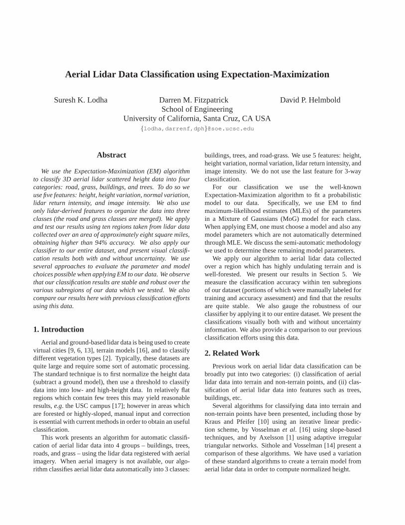
(a) Normalized Height (H) (b) Height Variation (HV) (c) Normal Variation (NV) (d) Lidar Return Intensity(LRI)

(e) Image Intensity (I)

Figure 1. The five feature images computed for Region 2.

Previous multiclass classification efforts include re-search by Axelsson [1], Maas [12], Filin [5], and Haalaand Brenner [7]. Most of these approaches are ad hocand based on heuristics. In addition, in most cases, resultsare presented for small regions without much discussion onthe overall quality of results obtained. Furthermore, mostof the previous work in classification of aerial lidar datahas concentrated on unsupervised clustering into a smallernumber of classes often resulting in coarse classification.Finally, these approaches often require substantial manualinput.

The most relevant previous work uses the Expectation-Maximization (EM) algorithm with a Mixture of GaussianModels to classify lidar data into four categories [3]. Thereare several differences between this previous work and thecurrent. First, the previous work requires the use of ad-ditional information – DEM data, co-registered with aeriallidar data. Second, the previous implementation of EM al-gorithm suffers from instability due to dependencies of thealgorithm on user-selected parameters, specifically,K, thenumber of components in the mixture model. We providedata to justify a semi-automatic method for determining thisvalue. Third, the previous work did not apply the result to alarge, untrained dataset (such as our entire dataset classifi-cation). Fourth, we use a different feature set. We introducenormal variation, which we will later find is very useful inour classification. Multiple return difference [3], which wasused as a feature in the previous work, is discarded as it wasnot found to be useful. Finally, as reported in Section 5,we obtain higher accuracy (better than 94%) in comparisonto the 66-84% accuracy reported in the previous work. Wealso compare our results to previous results using the SVMalgorithm to classify this data [11].

3. Data Processing

Our lidar dataset was acquired by Airborne1 Inc. Thedata was collected for approximately eight square miles of

target region using a 1064 nm laser at a pulse rate of 25KHz. The raw data consists of about 36 million points, withan average point spacing of 0.26 meters. We resampled thisirregular lidar point cloud onto a regular grid with a spacingof 0.5m using nearest-neighbor interpolation.

In addition, we use high-resolution (0.5ft/pixel) ortho-rectified gray-scale aerial imagery. We downsampled theaerial imagery to the same 0.5m/pixel resolution as the lidardata and registered the two.

3.1. Features

We have identified five features to be used for dataclassification purposes: normalized height, height variation,normal variation, lidar return intensity, and image intensity.

• Normalized Height (H): We computed the terrain el-evation data automatically from the aerial lidar datausing a variation of the standard DEM extraction al-gorithms [14]. The lidar data is normalized by sub-tracting terrain elevations from the lidar data.

• Height Variation (HV): Height variation is measuredwithin a 3×3 pixel(2.25m2) window and is calculatedas the absolute difference between the min and maxvalues of the normalized height within the window.

• Normal Variation (NV): We first compute the normalat each grid point using finite differences. Normalvariation is the average dot product of each normalwith other normals within a 11× 11 pixel (30.25m2)window. This value gives a measure of planarity withinthe window.

• Lidar Return Intensity (LRI): Along with the heightvalues, aerial lidar data contains the amplitude of theresponse reflected back to the laser scanner. We referto this amplitude as LRI.

2

• Image Intensity (I): Image intensity corresponds to theresponse of the terrain and non-terrain surfaces to vis-ible light. This is obtained from the gray-scale aerialimages.

All the five features have been normalized to integervalues between 0 and 255. Figure 1 shows images of thesefive features computed on Region 2.

3.2. Classes and Training

We classify the dataset into four groups: buildings(rooftops), trees or high vegetation (includes coniferousanddeciduous trees), grass or low vegetation (includes greenand dry grass), and road (asphalt roads, concrete pathwaysand soil). We also combine the road and grass classes toperform a 3-class labeling using only lidar-derived features.Ten different regions of the original dataset were segmentedand subregions of these were manually labeled for trainingand validation. The sizes of these ten regions vary from100,000 to 150,000 points; together they comprise about7% of our entire dataset. Roughly 25-30% of these regionswere manually labeled using a graphical user interface tocover the four classes adequately. However, the proportionsof the classes vary significantly from region to region.

4. The Expectation-Maximization Technique

Expectation-maximization (EM) [4] is a general methodfor fitting probability distributions which may contain unob-servable latent variables. Specifically, EM is often used tocompute maximum likelihood estimates (MLEs) of param-eters to probabilistic models being fit to data where someunobservable information prevents direct MLE. Within thecontext of probabilistic data classification by mixture mod-els, EM can be used to compute an MLE of the mixture pa-rameters for data when it is unclear from which componentof the mixture each datum was drawn from. EM alternatesbetween using the current parameter estimates to computethe likelihoods of each datum belonging to each compo-nent, and using these likelihoods to update the parameterestimates. Thus one can obtain an useful estimate of theprobability that a datum was drawn from some mixtureof distributions, even where it is impossible to know fromexactly which distribution the datum was sampled from.

4.1. Supervised Classification and EM

We have applied EM to a supervised classification prob-lem. Supervised classification requires a training set ofmeasurement (feature value) vectors as well as an associ-ated labeling assigning each feature vector to a particularclass. This training dataset is used to create a classifier withthe hope that it will perform well on unseen data whichis similar to the training data. Of course, an important

assumption here is that unseen data will be drawn from asimilar distribution to the training set; hence one shouldmake all practical efforts to ensure that this is the case.

Considering the task of assigning a class labelc, takenfrom a set of possible labelsC, to a feature vectorx, wemay compute the posterior probability ofx belonging tocusing Bayes’ rule:

P(c | x) =P(x | c)P(c)

P(x)(1)

whereP(x) = ∑c∈C P(x | c)P(c) andP(c) is the prior prob-ability of classc. Assuming no compelling prior infor-mation otherwise, it is common to assume thatP(c) foreach class is equal to 1/|C|. Although we do indeed havesomea priori knowledge of these values by our labeledtraining data, we have opted to leave them uniform. Thismore evenly distributes classifier accuracy over each class,yielding an increase in average per-class accuracy at theexpense of overall accuracy. The effect upon the three-wayclassification was small: an increase of 0.41% in mean per-class accuracy with a 0.16% decrease in overall accuracy. Inthe four-class instance this gave an increase in average per-class accuracy of 0.96% with a tradeoff of 1.04% in overallaccuracy.

For multiclass labeling, the label assigned tox will sim-ply be the valuec for whichP(c | x) is the largest. One mayobserve that in fact this implies that our algorithm apply EMto the data independently for each class, associatingx withthe class for which the trained classifier fits best. The onlyinformation still needed in order to perform classificationare the class-conditional densitiesP(x | c). These will beestimated, as is often the done, by using a mixture model;the model will be fit automatically by EM.

4.2. Model Choices and Parameters

As EM is a generic algorithm, we must choose an un-derlying model with which to describe our data as wellas choose all parameters for said model which are notautomatically determined. For our Mixture of Gaussians(MoG) model, this amounts to choosingK, the numberof Gaussians in the mixture. Modeling with a mixture ofGaussians is an appropriate choice for data which is createdby randomly perturbing prototypes. In this way a complexfeature distribution can be usefully approximated by a sim-pler, finite mixture. Analysis of our data through marginaland joint histograms of feature values have convinced usthis model is a reasonable choice for our task. We further re-strict our model to independent Gaussians over each feature(zero-covariance) in order to circumvent the numerical pre-cision problems inherent in fitting an arbitrary MoG modelover all features. This restriction had no appreciable effecton measured performance: comparing the results of ourleave-one-out test using independent as opposed to arbitrary

3

1 2 3 4 5 6 7 8 9 11 13 15 18 21 24 27 30 350.9

0.91

0.92

0.93

0.94

0.95

0.96

0.97

0.98

Number of clusters K

Ove

rall

accu

racy

%

4−Class Mean Score4−Class Score Deviation3−Class Mean Score3−Class Score Deviation

Figure 2. Mean overall MCCV classification accuracy over 10random partitionings of the training data as different values ofKare selected.

distributions using identicalK values showed an overalldifference less than 0.2% in overall classification accuracyin both three- and four-way classification. Furthermore, werestricted the variance values of these Gaussians to at least.25 for each feature (recall that our features have integervalues on the range[0,255]). This is to avoid the casewhere a Gaussian is fit to a very few feature values withvariance approaching zero, leading to degenerate (infinite)likelihoods.

We model the probability of observing a set of measure-mentsx given labelingc as

p(x | c) =K

∑j=1

PjG(x | µ j ,Σ j ) (2)

The parameters for each of the Gaussians,(µ j ,Σ j), as wellas their respective mixing coefficientsPj will be iterativelydetermined by EM automatically after manually choosingthe remaining model parameterK, the number of compo-nents in the mixture.

Unfortunately the choice ofK is not a completelystraightforward task. The model needs to describe thedata as accurately as is practical, yet one may always addadditional Gaussians to create a new model which performsat least as well. At some point the overfitting of an overlycomplex model must outweigh the benefit gained from acloser fit. Although research is ongoing in the area ofautomatically determining an optimal value forK, we havechosen one strong candidate criteria, theBayesian Informa-tion Criterion (BIC), to aid in deciding the best value asdescribed in [8]. Visual and numerical classification resultsjustify this decision. BIC, like similar metrics such as theAkaike Information Criterion, weigh increase in training

1 2 3 4 5 6 7 8 9 11 13 15 18 21 24 27 30 35

2

4

6

8

10

12

x 105

Number of clusters K

BIC

val

ue

4−Way BIC Per Class vs K

TreeGrassRoadBuilding

Figure 3. Mean BIC value calculated using 10 random partition-ings of the training data for each class as different values of K areselected. The local minima have been marked.

data log-likelihood against increased model complexity toyield a single function which may be minimized in order toautomatically determine appropriate parameter values.

Training data log-likelihoods were taken from tests usingMonte Carlo Cross-Validation(MCCV) [15]. MCCV is atechnique for cross-validating training data using the aver-age of a series of tests over random partitions of the data.This method of testing is particularly suited to evaluatingmodel parameters, as overfitting problems should be morereadily apparent relative to other standard train-test methodssuch asv-fold Cross-Validation. Although Smyth reportssuccessfully using MCCV to identify optimal values forK[15], we found that MCCV alone was unable to identify areasonable value. Instead, we used the log-likelihood valuesresulting from the MCCV tests in our calculation of BIC,which yielded quite reasonable results.

Shown in Figure 2 are the results from MCCV testingusing equal values ofK for each class. As can be seen,even at large values ofK, slight increases in accuracy areobserved. Thus we cannot rely upon MCCV accuracyresults alone. Instead, we use the log-likelihoods resultingfrom these tests to compute the per-class BIC values plottedin Figure 3. Minimizing the BIC gave reasonable valuesof K for each class which we used for all results discussedin Section 5. Finally, we may compare various values ofK by examining the resulting fit when trained upon ourdata. Figure 4 shows the resulting distribution upon thelidar return intensity feature after training the buildingclasswith various values ofK. Clearly, the higher values ofKfit the data better than the lowest, although the differencebetween the highest values is much less significant. In the4-class case, the values ofK selected were 9, 9, 7, and 8for buildings, trees, road, and grass, respectively. In the3-

4

0 2550

0.005

0.01

0.015

0.02

0.025

0 2550

0.005

0.01

0.015

0.02

0.025

0 2550

0.005

0.01

0.015

0.02

0.025

0 2550

0.005

0.01

0.015

0.02

0.025

Figure 4. The fit obtained upon the lidar return intensity feature for the building class. Left to right:K equal to 1, 3, 9, and 30.

class case, values of 9, 9, and 8 for buildings, trees, androad-grass were used.

5. Results and Analysis

All accuracy results presented in this section are createdusing leave-one-out testing. For leave-one-out tests, 9 ofour10 labeled regions serve as the source of training samplesused as input to our EM algorithm. The accuracy of theresulting classifier is then measured upon all labeled pointswithin the remaining (held out) region. For labeled datain the 9 training regions, 1/8 of the points are randomlysampled as training input. We have found that in practicedownsampling the training data to as little as one tenththe available size has no significant effect upon our results.When calculating the overall leave-one-out accuracy for all10 regions, we take the sum of the correctly classified pointsin each region and divide it by the total number of points inall regions,i.e. smaller regions contribute less to the overallscore.

We report two types of accuracy: sample- and class-weighted. Sample-weighted accuracy is simply the percent-age of correctly classified points. Class-weighted accuracyis the mean percentage of correctly classified points fromeach class. That is, per-class accuracies are computed andthen averaged to compute class-weighted accuracy. Some-times a certain class is the most interesting yet it is relativelyuncommon in the data. Class-weighted accuracy is useful inidentifying cases where a rare classes is poorly classified yetoverall accuracy is still high, which might be undesirable.

We now present our results both visually and numeri-cally. Recall that for these tests 9, 9, 7 and 8 Gaussians werefit to the building, tree, road, and grass classes respectively(9, 9 and 8 Gaussians for building, tree and road-grass in the3-class case). Table 1 presents leave-one-out test accuracyfor each region and overall. We achieve an overall sample-weighted accuracy of better than 94% in the 4-class caseand better than 97% in the 3-class case. The overall class-weighted accuracy results are similar, however some ofthe test regions performed significantly poorer than others.This can be attributed to localized differences in featuresin these two regions. Luminance and lidar return intensityboth varied significantly in some classes over various areas.Particularly, the grass class (in the 4-way classification)and

Region5 features, 4 classes 3 features, 3 classes

class-weighted

sample-weighted

class-weighted

sample-weighted

baskin 74.21 % 92.95 % 86.17 % 95.21 %c8 93.26 % 94.62 % 98.02 % 97.80 %crown 91.60 % 95.47 % 95.88 % 95.62 %efh 94.32 % 96.27 % 96.52 % 97.95 %fsh 93.60 % 94.52 % 96.73 % 96.59 %oakes 93.82 % 93.87 % 96.35 % 98.44 %pc 89.39 % 88.25 % 96.08 % 97.08 %porter 95.48 % 95.75 % 97.44 % 96.21 %sh 76.25 % 93.83 % 86.44 % 95.25 %ta 94.46 % 94.35 % 98.66 % 98.54 %Overall 93.83 % 94.31 % 96.98 % 97.12 %

Table 1. Leave-one-out test accuracy: overall and for each of the10 regions.

5/4 Tree Grass Road Bldg. Error ITree 96.61 0.24 1.09 2.06 3.39Grass 0.35 91.44 6.92 1.30 8.57Road 0.59 7.41 91.39 0.61 8.61Bldng. 3.81 0.06 0.26 95.87 4.13Error II 4.75 7.71 8.27 3.97

3/3 Tree Bldng. Road-Grass Error ITree 96.36 2.91 0.73 3.64Bldng 3.47 96.44 0.09 3.56Road-Grass 0.59 1.27 98.14 1.86Error II 4.06 4.18 0.82

Table 2. Classification accuracy and Type I/II error resultsorga-nized by class, for 5 features/4 classes and 3 features/3 classes.These are the cumulative results over all 10 test regions.

the merged road-grass class (in the 3-way classification)were poorly classified in the two regions due to these dif-ferences. This is understandable as the grass points in thesetwo regions were significantly darker than in other areas.Sample-weighted accuracy also dropped to 88.25% in oneof the ten regions during the 4-way classification. This isdue to a relative abundance of the most commonly confusedclasses, road and grass, in this region. Since these classeswere merged in the 3-class instance, this disparity is notpresent in the 3-way results.

Table 2 presents the confusion matrix for the overallleave-one-out results. As mentioned, in the 4-class caseroad and grass are the most commonly confused classes.

5

Figure 5. Leave-one-out classification results for the College 8 region: (far left) 4-way classification using 5 features; (2nd from left) 4-wayconfidence-rated classification using 5 features; (2nd fromright) 3-way classification using 4 features; (far right) 3-way confidence-ratedclassification using 4 features.

Figure 6. Per-class density images for each class on the College 8 region using the leave-one-out test with 4 classes; left to right the imagesshow the probabilities for building, tree, road and grass.

Another significant source of error in the 4-way classifica-tion were building points misclassified as tree. Buildingswere much easier to discern from the cumulative road-grassclass than from the road and grass classes independently.This leaves confusion between buildings and trees as theremaining significant source of error in the 3-way classifi-cation.

As mentioned in Section 2, these accuracies are signifi-cantly higher than our previously reported results using theEM algorithm [3]. Previously reported accuracies rangedfrom 66% to 84% over the 10 testing regions, we nowobtain higher than 94% overall accuracy on these regions.Also, when applying the previous EM classifiers to newerfeature data, we noticed that the results were unstable andhad difficulty reobtaining similar accuracy rates. Our newerEM classifier is more stable and accurate. This increasein stability and accuracy can primarily be attributed to ourimproved feature data and automatic parameter selection.In comparing our current EM results to our previous resultsusing SVM [11] we observe that both accuracy rates and

sources of error are similar. Specifically, we observe that inboth cases confusion between road and grass is the primarysource of error, with building points misclassified as treebeing another significant source of error. This leads us toconclude that classification using EM is not our only viablechoice. From this comparison we also conclude that themost promising route to improving classification accuracyis in further refinement of our feature data. Particularly, ourcurrent height-based features are somewhat ineffectual indiscerning between road and grass points, and, in certaincases, between tree and building points.

We also present visual classification results for one ofour 10 subregions as well as for our entire dataset, withand without uncertainty. In these figures points classified asbuilding are shown in blue, tree points are shown in green,and road and grass points are shown in brown and yellow,respectively. For 3-way output the road-grass points areshown in yellow. Also, in confidence-rated output, colorsare scaled by their classification certainty, that is, darkerpoints are to be trusted less. This confidence rating is taken

6

as the ratio of the difference between the most and nextmost probable to the most probable classification. Figure 5shows visual classification results for one of our ten subre-gions. Recall that less than 5% of points in the remaining9 subregions was used for training. Buildings are clearlydistinguishable, as are trees and the surrounding roads. Themost evident source of error, visually, are building edgeslabeled as tree, as well as tree points mislabeled as building.In the images with uncertainty output these are typicallymarked by lower confidence. This visual evaluation cor-responds well with the insight gained from the confusionmatrix presented in Table 2. Also evident is that in certainareas no good labeling for our algorithm exists,e.g. carsin parking lots which are classified as buildings and tenniscourts which are classified as roads. These points, too, areassigned low classification confidence. Further research isnecessary in order to elegantly handle these cases. Onepossibility might be to assign an ‘other’ labeling to allobjects for which no useful classification exists.

Figure 7 presents a visualization of the classification re-sults for all the points within our entire dataset. We observethe same level of visual quality in these results as obtainedin the testing subregions. Specifically, roads, buildings andareas of forest are clearly visible, with the confidence-ratedoutput guiding the eye toward the most reliable portionsof the classification. We also notice some spatio-temporalinconsistencies in these results. For example, in the upper-left there is an area of mixed building and tree pointswith low confidence. This area contained trailers duringlidar collection which were not present during aerial imagecollection. The classifier used for this output was trainedupon a random sampling of 1/8 the labeled data in all 10subregions. This training data comprised less than 1% of thetotal number of classified points. Clearly our results extendfrom the testing subregions into nearby geographical areasquite successfully. Only further comparison with additionaldatasets will tell the limits of the extensibility of classifiersfrom one region to another.

6. Conclusions and Future Directions

We have presented a method of applying the EM algo-rithm to the classification of aerial lidar data. We do so quitesuccessfully with an overall accuracy rate of greater than94%, which is better than our previously reported results.Our visual classification results demonstrate intuitivelytheeffectiveness of our technique. The confidence-rated vi-sual output clearly demonstrates the relative strengths andweaknesses in our classification. Comparing our resultsreported here with previous classification efforts upon thesame data lends valuable insight into the relative strengthsand weaknesses of these approaches. There are many futurepossibilities for extending our work. These include theuse of additional features, extension into different sets of

classes, the enforcement of spatial coherency constraints, aswell as many post-processing possibilities such as buildingfootprint extraction and virtual walk-throughs.

Acknowledgements

This research is partially supported by the Multi-disciplinary Research Initiative (MURI) grant byU.S. Army Research Office under Agreement NumberDAAD19-00-1-0352, the NSF grant ACI-0222900, and theNSF-REU grant supplement CCF-0222900.

References

[1] P. Axelsson. Processing of laser scanner data -algorithms andapplications.ISPRS Journal of Photogrammetry and RemoteSensing, 54(2-3):138–147, 1999.1, 2

[2] J. B. Blair, D. L. Rabine, and M. A. Hofton. The laservegetation imaging sensor: a medium altitude, digitsation-only, airborne laser altimeter for mapping vegetaion andtopography.ISPRS Journal of Photogrammetry and RemoteSensing, 54:115–122, 1999.1

[3] A. P. Charaniya, R. Manduchi, and S. K. Lodha. Supervisedparametric classification of aerial lidar data.IEEE workshopon Real-Time 3D Sensors, pages 25–32, June 2004.2, 6

[4] A. Dempster, N. Laird, and D. Rubin. Maximum likelihoodfrom incomplete data via the EM algorithm (with discus-sion). Journal of the Royal Statistical Society, Series B,39(1):38, 1977.3

[5] S. Filin. Surface clustering from airborne laser scanning. InISPRS Commission III, Symposium 2002 September 9 - 13,2002, Graz, Austria, 2002.2

[6] C. Frueh and A. Zakhor. Constructing 3D city models bymerging ground-based and airborne views. InIEEE Con-ference on Computer Vision and Pattern Recognition, June2003.1

[7] N. Haala and C. Brenner. Extraction of buildings and treesin urban environments.ISPRS Journal of Photogrammetryand Remote Sensing, 54(2-3):130–137, 1999.2

[8] T. Hastie, R. Tibshirani, and J. Friedman.The Elements ofStatistical Learning: Data Mining, Inference, and Predic-tion. Springer, 2001.4

[9] J. Hu, S. You, and U. Neumann. Approaches to large scaleurban modeling. IEEE Computer Graphics and Applica-tions, 23(6):62–69, November/December 2003.1

[10] K. Kraus and N. Pfeifer. Determination of terrain modelsin wooded areas with airborne laser scanner data.ISPRSJournal of Photogrammetry and Remote Sensing, 53:193–203, 1998.1

[11] S. Lodha, E. Kreps, D. Helmbold, and D. Fitzpatrick. AerialLiDAR Data Classification using Support Vector Machines(SVM). In Third International Symposium on 3D DataProcessing, Visualization and Transmission, 2006.2, 6

[12] H.-G. Maas. The potential of height texture measures for thesegmentation of airborne laserscanner data.Fourth Interna-tional Airborne Remote Sensing Conference and Exhibition,

7

Figure 7. Classification of the entire dataset using (upper half) 4 classes and 5 features and (lower half) 3 classes and 3 features, without(left) and with (right) confidence rating.

8

21st Canadian Symposium on Remote Sensing:Ottawa, On-tario, Canada, 1999.2

[13] W. Ribarsky, T. Wasilewski, and N. Faust. From urbanterrain models to visible citites.IEEE Computer Graphicsand Applications, 22(4):10–15, July 2002.1

[14] G. Sithole and G. Vosselman. Comparison of filtering algo-rithms. InISPRS Commission III, Symposium 2002 Septem-ber 9 - 13, 2002, Graz, Austria, 2002.1, 2

[15] P. Smyth. Clustering using monte carlo cross-validation.In Knowledge Discovery and Data Mining, pages 126–133,1996.4

[16] G. Vosselman. Slope based filtering of laser altimetry data.International Archives of Photogrammetry and Remote Sens-ing, XXXIII, Amsterdam, 2000, 2000.1

[17] S. You, J. Hu, U. Neumann, and P. Fox. Urban site modelingfrom lidar. In Second International Workshop on ComputerGraphics and Geometric Modeling, 2003.1

9