aero engine technology
DESCRIPTION
Some calculations on working of aircraft engineTRANSCRIPT

21 November 2013
Aero engine Technology Assignment 4
Akshay R Kulkarni
Student Number- 4327837
Aero engine Technology 2013
Assignment 4 Page 2
Table of Contents Table of Contents .................................................................................................................................... 2
1 Problem Statement ......................................................................................................................... 4
2 Assumptions .................................................................................................................................... 4
3 Procedure ........................................................................................................................................ 5
3.1 Part 1 ....................................................................................................................................... 5
3.1.1 Question 1 ....................................................................................................................... 5
3.1.2 Answer ............................................................................................................................ 5
3.1.3 Question 2 ....................................................................................................................... 6
3.1.4 Answer ............................................................................................................................ 6
3.1.5 Question 3 ....................................................................................................................... 7
3.1.6 Answer ............................................................................................................................ 7
3.2 Part 2 ....................................................................................................................................... 7
3.2.1 Question .......................................................................................................................... 7
3.2.2 Answer ............................................................................................................................ 8
4 Results and Conclusion ................................................................................................................... 9
4.1 Part 1 ...................................................................................................................................... 9
4.2 Part 2 .................................................................................................................................... 10
4.2.1 A comment on Degree of reaction................................................................................ 10
4.2.2 Turbine blade design using turbine GUI ....................................................................... 11
5 Appendix ....................................................................................................................................... 14
Aero engine Technology 2013
Assignment 4 Page 3
Table of figures Figure 1: General velocity triangle .......................................................................................................... 5
Figure 2 : Velocity triangle for the turbine blade .................................................................................... 9
Figure 3: Blade profile at the hub ......................................................................................................... 11
Figure 4: Blade Profile at Mid-span ....................................................................................................... 12
Figure 5: Blade profile at the shroud .................................................................................................... 13

Aero engine Technology 2013
Assignment 4 Page 4
1 Problem Statement The flow leaving an axial turbine stator blade row has a velocity 300m/s at an angle of 40°.
The rotational speed of the rotor is 5000rpm. The flow leaving the rotor blade row also has
a relative velocity of 300 m/s at a relative angle of -40°. Neglect any losses and radial
velocities and assume that the axial velocity is constant throughout the stage. For part 1
only: the stage is not a repetition stage (c1 ≠ c3). The first part of the question deals with the
velocity triangle, the mass flow rate and the power. The second on the other hand deals
with the design of blade and blade height effects.
𝛼2 = 40° 𝛽3 = −40° 𝑊3 = 300𝑚
𝑠 𝐶2 =
300𝑚
𝑠
2 Assumptions Leakages in the turbine are ignored
Isentropic relations are assumed in the turbine working
Ideal gas behaviour
The given temperatures and entrance angles are assumed at the mid-span
𝐶𝑥values are assumed constant
Radial velocities are ignored
In part 2 of the problem, repetition stage is assumed
In part 2, free vortex system is assumed
Secondary flows are ignored
Tip leakage is ignored

Aero engine Technology 2013
Assignment 4 Page 5
3 Procedure
3.1 Part 1
3.1.1 Question 1 Calculate the relative flow angle at the rotor inlet and the absolute flow angle at rotor exit. Draw the
velocity triangles.
3.1.2 Answer For the analysis of velocity triangles at the inlet and exit of rotor blades, the general trend used
(schematic reference ) is the following1:
Figure 1: General velocity triangle
Ofcourse, the actual2 triangle depends on the relative values of 𝛼, 𝛽, 𝐶 𝑎𝑛𝑑 𝑊 . The determination of
this depends on simple rules of geometry and relative velocity. The following equations are used to
determine the requisite parameters.
𝑡𝑎𝑛 𝛽2 = 𝑡𝑎𝑛 𝛼2 −𝑈
𝐶𝑥
𝐶𝑥 is the cos component of the absolutevelocity given as :
1 Obtained directly from lecture slides
2 The actual velocity triangles are drawn in the result section. The velocity triangle given here is for schematic
reference only.

Aero engine Technology 2013
Assignment 4 Page 6
𝐶𝑥 = 𝐶2 𝑐𝑜𝑠 𝛼2
Where, U is the velocity at the circumference of the turbine. The multiplication of angular velocity
with the circuference yilds the circumferential velocity. This is given by,
𝑈 =𝜔 2𝜋𝑟
60
Using the three relations above, the relative flow angle 𝛽2 at the inlet can be determined.
Consequently, using the relation given below, 𝑊2 can be determined.
𝐶2 𝑐𝑜𝑠 𝛼2 = 𝑊2 𝑐𝑜𝑠 𝛽2
Similarly, to determine the absolute flow angle and the absolute velocity at the outlet of the rotor is
given by,
tan 𝛼3 = tan 𝛽3 +𝑈
𝐶𝑥
𝐶3 𝑐𝑜𝑠 𝛼3 = 𝑊3 𝑐𝑜𝑠 𝛽3
3.1.3 Question 2 Compute the mass flow rate for a given constant mean radius of 0.5m, a constant span 0.3m, a
stagnation temperature of 1400K and a stagnation pressure of 30bar. The gas constant is 287[J/kg/K]
and the ratio of specific heats is 1.34.
3.1.4 Answer The answer to this question begins with the assumption that the conditions of temperature given
are indicative of pressure at the inlet of the rotor. Mass flow rate is directly given as the product of
density, area and velocity. Which comes from the equation of continuity. The equation is given as
follows:
𝑚 = 𝜌𝑉𝐴
The effective area under consideration is the area between the hub and the shroud. Since the
turbine always includes a circular rotation, the equation is given as :
𝐴 = 𝜋𝑟𝑠ℎ𝑟𝑜𝑢𝑑2 − 𝜋𝑟ℎ𝑢𝑏
2
The density calculation involves certain difficult because the density so obtained from ideal gas
equation is the static density. So, appropriate conversion needs to be used to obtain the dynamic
density. This done using the following equations.
𝜌0 =𝑃0
𝑅 𝑇0

Aero engine Technology 2013
Assignment 4 Page 7
where, the subscript 0 indicates static values of the given variable. TO obtain the dynamic value, the
following equation is used:
𝜌0
𝜌= (
𝑇0
𝑇)
1
𝛾−1
The static temperatures are not know too. So, we use the energy equation to obtain static
temperature. The equation is given as :
𝐶𝑝𝑇0 = 𝐶𝑝𝑇 +𝐶2
2
2
where,
𝐶𝑝 =𝛾𝑅
𝛾 − 1
3.1.5 Question 3
What is the power output of this turbine stage?
3.1.6 Answer Euler equation is used to determine the power generated in the turbine. The tangential velocities
are obtained using the following formulae.
𝑃 = 𝑚 𝑈(𝐶𝜃3 − 𝐶𝜃2)
where,
𝐶𝜃2 = 𝐶2𝑠𝑖𝑛𝛼2
𝐶𝜃3 = 𝐶𝑥𝑡𝑎𝑛𝛼3
3.2 Part 2
3.2.1 Question
Design the 3D stator and rotor geometry based on a free vortex approach.
Draw the velocity triangles at the hub, mid span and at the shroud.
Compute the flow coefficient, degree of reaction and the loading factor as a function of the blade height. Comment on the degree of reaction at the hub and the one at the shroud (blade tip).
Use the MATLAB program “turbineGUI” to draw the vane/blade profiles.

Aero engine Technology 2013
Assignment 4 Page 8
3.2.2 Answer The free vortex design bases itself on the premise that the stagnation enthalpy and the axial velocity
are constant . It is also interesting to note that at any point, along the turbine blade height, using
the constants A1 and A2, the power generated remains constant. The following constants can thus
be defined:
𝐴1 = 𝑟𝑚𝐶𝜃1
𝐴2 = 𝑟𝑚𝐶𝜃2
Also, the free vortex design implies 𝐶𝑥 remains constant. To add to that, the question clearly states
that 𝐶1 = 𝐶3 owing to the repetition of the stages. Using the tangential velocities and simple rules
of trigonometry and referring to the lecture slides, following relations as illustrated below are used
to calculate the angles at various stations. The radius r used below includes the different radii at hub
mid-span and shroud.
𝛼1 = 𝑡𝑎𝑛−1𝐴1
𝑟𝐶𝑥
𝛼2 = 𝑡𝑎𝑛−1𝐴2
𝑟𝐶𝑥
𝛽1 = 𝑡𝑎𝑛−1
𝐴1
𝑟− Ω𝑟
𝐶𝑥
𝛽2 = 𝑡𝑎𝑛−1
𝐴2
𝑟− Ω𝑟
𝐶𝑥
From the angles determined, we can easily determine the relative and absolute velocities using basic
trigonometry as shown in the equations below.
𝐶1 =𝐶𝑥
𝑐𝑜𝑠𝛼1
𝑊1 =𝐶𝑥
𝑐𝑜𝑠𝛽1
𝐶2 =𝐶𝑥
𝑐𝑜𝑠𝛼2
𝑊2 =𝐶𝑥
𝑐𝑜𝑠𝛽2
Once the fundamental angles and velocities are determined as discussed in the equations above, the
performance characteristic can be described by equations shown below:
𝜙 =𝐶𝑥
𝑈
𝜓 = −1 + 𝜙(𝑡𝑎𝑛 𝛼2 − tan 𝛽3)
𝑅 =1
2−
𝜙
2(𝑡𝑎𝑛 𝛼2 + tan 𝛽3)
These performance characteristics can be further used in the MATLAB code provided to determine
the 3 d blade geometry.

Aero engine Technology 2013
Assignment 4 Page 9
4 Results and Conclusion
4.1 Part 1 Following are the results required for the part 1 of the assignment. The calculation for this is carried
out in the MATLAB program3 and the values so asked are tabulated below.
Units Values
𝛽2
-16.7°
𝛼3 16.7° V (m/s) 229.81
A (𝑚2) 0.9425
𝜌 𝑘𝑔
𝑚3 6.859
T (K) 1360.2 Cp(J/kg K) 1131.1
𝑚 (kg/s) 1485.7
P (W) -4.81*107
It is interesting to note that the power so obtained is negative. This can be explained as the power
removed from the gas due to the decrease in its kinetic energy. Which equivalently is added to to
the turbine. Thus, the negetive sign makes sense. Drawn below is the actual velocity triangle for the
question in part 1.
Figure 2 : Velocity triangle for the turbine blade
3 The MATLAB program so used is attached in the appendix

Aero engine Technology 2013
Assignment 4 Page 10
4.2 Part 2
Shown below are the values of various parameters as indicated at different points on the turbine
blade. These are calculated with the formulae described in the procedure4.
4.2.1 A comment on Degree of reaction The degree of reaction relates the change in enthalpy in the rotor to the change in enthalpy of the
stage. If we observe the degree of reaction at various points on the turbine blade height, we observe
an increase with increase in radius. This can be explained by the fact that increase in the radius
results increase in the value of U as can be seen from the equations detailed in procedure. This leads
to increase in enthalpy in the rotor and consequently the stage. But, the increase in enthalpy in rotor
is much more than the increase in enthalpy in the entire stage and thus we see the increase in
4 The MATLAB program for the calculation is attached in the appendix
Hub Mid-span Shroud
Radius (m) 0.35 0.5 0.65
𝜷𝟏(rad) -0.35327 -0.69813 -0.8961
𝜷𝟐(rad) 0.381614 -0.29153 -0.696
𝜷𝟑(rad) -0.35327 -0.69813 -0.8961
𝜶𝟏(rad) 0.404992 0.291533 0.22686
𝜶𝟐(rad) 0.875531 0.698132 0.573178
𝜶𝟑(rad) 0.404992 0.291533 0.22686
W1(m/s) 244.9391 300 367.8996
W2(m/s) 247.6264 239.9377 299.4654
W3(m/s) 244.9391 300 367.8996
C1(m/s) 250.0402 239.9377 235.8566
C2(m/s) 358.7529 300 273.5281
C3(m/s) 250.0402 239.9377 235.8566
𝝓 1.254032 0.877822 0.675248
𝝍 0.965634 0.473161 0.279977
R -0.02041 0.5 0.704142

Aero engine Technology 2013
Assignment 4 Page 11
degree of reaction. As is seen from the above table, there is a negetive value for degree of reaction
at the root of the blade. This non-intuitive value can be explained on the fact that the enthalpy in
the rotor increases by a very small amount that is to say the flow at the hub behaves differently as
compared to the mid-span and shroud. Here a very small compression is experienced instead of the
usual expansion of gases.
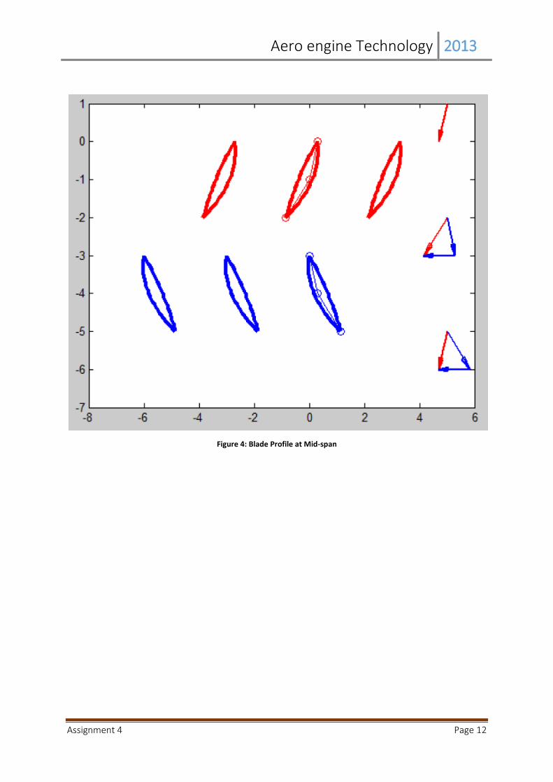
4.2.2 Turbine blade design using turbine GUI
Shown below are the turbine shapes at hub shroud and the mid-span of the turbine blade. A n
observation of the same reveals that the blades get skewed as we move from hub to shroud.
Figure 3: Blade profile at the hub
Aero engine Technology 2013
Assignment 4 Page 12
Figure 4: Blade Profile at Mid-span

Aero engine Technology 2013
Assignment 4 Page 13
Figure 5: Blade profile at the shroud

Aero engine Technology 2013
Assignment 4 Page 14
5 Appendix % Aero Engine Technology 4
clc %% Input: c2=300; %Absolute vel 2 [m/s] a2=40*(pi/180); %Absolute angle 2 [rad] omega=5000; %Rotational speed [RPM] w3=300; %Rotor relative velocity 3 [m/s] b3=-40*(pi/180); %Relative angle 3 [rad] r=0.3; %Span radius [m] rmean=0.5; %Mean radius [m] R=287; %Gas constant [J/kg/K] t0=1400; %Stagnation temperature [K] P0=30*10^5; %Stagnation Pressure [Pa] Y=1.34; %Specific heat ratio [J/kg K] %% Question 1.1: cx=c2*cos(a2); U2=(omega/60)*2*pi*rmean; %? b2=(atan(tan(a2)-(U2/cx))); U3=U2; a3=(atan(tan(b3)+(U3/cx))); w2=cx/cos(b2); %% Question 1.2: rin=rmean-r/2; rout=rmean+r/2; A=pi*(rout^2-rin^2); V=cx; cp=(Y*R)/(Y-1); T=t0-c2^2/(2*cp); rho0=P0/(R*t0); rho=rho0*(t0/T)^(-1/(Y-1)); m=rho*V*A; %% Question 1.3: ctan2=c2*sin(a2); ctan3=tan(a3)*cx; P=m*U3*(ctan3-ctan2); %% Question 2
c3=sqrt(ctan3^2+cx^2); c1=c3; a1=acos(cx/c1); ctan1=c1*sin(a1);
A1=ctan1*rmean A2=ctan2*rmean A3=A1
for rvecmm=1: 1 :3; if rvecmm==1 rvec(rvecmm)=0.35 elseif rvecmm==2 rvec(rvecmm)=0.5 else rvec(rvecmm)=0.65 end
U(rvecmm)=(omega/60)*2*pi*rvec(rvecmm)

Aero engine Technology 2013
Assignment 4 Page 15
newa2(rvecmm)=atan(A2/(rvec(rvecmm)*cx)) newa1(rvecmm)=atan(A1/(rvec(rvecmm)*cx)) newa3(rvecmm)=newa1(rvecmm) newb3(rvecmm)=atan(((A3/rvec(rvecmm))-(rvec(rvecmm)*5000*(2*pi/60)))/cx) newb1(rvecmm)=newb3(rvecmm) newb2(rvecmm)=atan(((A2/rvec(rvecmm))-(rvec(rvecmm)*5000*(2*pi/60)))/cx)
neww1(rvecmm)=cx/cos(newb3(rvecmm)) neww2(rvecmm)=cx/cos(newb2(rvecmm)) neww3(rvecmm)=neww1(rvecmm)
newc1(rvecmm)=cx/cos(newa1(rvecmm)) newc2(rvecmm)=cx/cos(newa2(rvecmm)) newc3(rvecmm)=newc1(rvecmm)
phi(rvecmm)=(cx/U(rvecmm)) psi(rvecmm)=-1+phi(rvecmm)*(tan(newa2(rvecmm))-tan(newb3(rvecmm))) R0(rvecmm)=0.5-((phi(rvecmm)/2)*(tan(newa2(rvecmm))+tan(newb3(rvecmm)))) end