aeroacoustic optimization of a low-speed fan - ulisboa · aeroacoustic optimization of a low-speed...
TRANSCRIPT

Aeroacoustic Optimization of a Low-Speed Fan
João Miguel Rebelo Branco
Thesis to obtain the Master of Science Degree in
Aerospace Engineering
Supervisor: Prof. André Calado Marta
Examination Committee
Chairperson: Prof. Fernando José Parracho LauSupervisor: Prof. André Calado MartaMember of the Committee: Prof. Luís Manuel Braga da Costa Campos
June 2015

ii

I would like to dedicate this work to all the people who helped me become the person I am today.
iii

iv

Acknowledgments
First of all, I would like to thank Prof. Andre Calado Marta for his teachings, patience, availability and for
being an overall excellent supervisor throughout the development of this thesis. Also, the author would
like to express a special appreciation to Prof. Luıs Braga Campos for his valuable input and scientific
review during various stages of this work. I have to thank the support of my family, especially my mother
and my father, for being so supportive and always present for the good and the bad and for making
me believe that every goal is attainable, one step at a time. I have also to thank my colleague Simao
Santos Rodrigues for his patience and guidance towards the understanding of the original aeroacoustic
framework. On a final note, I have to thank my long time teacher, Prof. Cesina Bona, without whom this
work and all my present accomplishments would not be possible.
v

vi
Resumo
O uso de sistemas de ar condicionado registou um crescimento nas ultimas decadas devido ao au-
mento do poder de compra no mundo desenvolvido e ao conforto que estes sistemas proporcionam,
tendo aumentado tambem a consciencializacao sobre o seu impacto negativo na saude publica. Muitos
estudos foram realizados para prever e minimizar o ruıdo das ventoinhas presentes nestes sistemas.
Neste trabalho, uma ferramenta aeroacustica baseada na teoria de elementos de pas-momento linear
para efeitos de previsao aerodinamica foi acoplado aos modelos aeroacusticos baseados nos trabalhos
de Carolus et al (2007) e Brooks et al (1989) e ao XFOIL para a computacao dos parametros de camada
limite. Esta ferramenta foi validada usando dados experimentais de uma ventoinha axial conhecida e
os nıveis de ruıdo de um modelo de ventoinha AC foram determinados. A pa foi parametrizada usando
curvas de Bezier para descrever as distribuicoes de corda e torcao e os perfis 2D. Foi realizado um
estudo parametrico onde se estudou o impacto do diametro e do numero de pas no ruıdo. O codigo
aeroacustico foi acoplado ao modulo de optimizacao pyOpt e usando o algoritmo genetico NSGA-II,
um conjunto de optimizacoes mono e multi-objectivo foram realizadas na ventoinha de base, usando a
corda, torcao e curvatura como design variables. Verificou-se uma reducao maxima de 4.1% no ruıdo
e um aumento maximo de 5.3% na eficiencia da ventoinha.
Palavras-chave: Projecto Aeroacustico, Reducao de Ruıdo, Ar Condicionado, Optimizacao
Multi-Objectivo, Algoritmos Geneticos.
vii

viii

Abstract
The use of air conditioning systems has increased in the recent decades due to the growth of the
purchasing power in the developed world and the confort they provide, whereas the awareness regarding
the negative health impacts of these systems has also increased. Many studies were conducted to
predict and minimize the noise of the fans present in most of these systems. In this work, a noise
prediction framework based on the Blade Element Momentum method for aerodynamic prediction was
coupled to the empirical aeroacoustic models based on the works of Carolus et al (2007) and Brooks et
al (1989) and to XFOIL for boundary layer parameter calculations. This framework was validated against
experimental data of a known axial impeller and an existing air conditioning fan model was analyzed and
its baseline noise values were characterized. A blade parameterization method was developed where
the chord and twist distributions and airfoil sections were described by Bezier curves. A parametric
study to determine the impact of fan diameter and blade number on the produced noise was conducted.
The aeroacoustic code was coupled to the optimization framework pyOpt, and by using the NSGA-
II genetic algorithm, a set of single and multi-objective optimizations, with chord, twist and curvature
as design variables were performed on the baseline fan and on the minimum noise fan resultant from
the parametric study. The optimal solutions indicated a maximum reduction of 4.1% in noise and a
maximum increase of 5.3% in efficiency. Introducing diameter and blade number changes, a significant
noise reduction is possible but with a moderate aerodynamic penalty.
Keywords: Aeroacoustic Design, Noise Reduction, Air Conditioning, Multi-objective Optimiza-
tion, Genetic Algorithms
ix

x

Contents
Acknowledgments . . . . . . . . . . . . . . . . . . . . . . . . . . . . . . . . . . . . . . . . . . . v
Resumo . . . . . . . . . . . . . . . . . . . . . . . . . . . . . . . . . . . . . . . . . . . . . . . . . vii
Abstract . . . . . . . . . . . . . . . . . . . . . . . . . . . . . . . . . . . . . . . . . . . . . . . . . ix
List of Tables . . . . . . . . . . . . . . . . . . . . . . . . . . . . . . . . . . . . . . . . . . . . . . xiii
List of Figures . . . . . . . . . . . . . . . . . . . . . . . . . . . . . . . . . . . . . . . . . . . . . xvii
Nomenclature . . . . . . . . . . . . . . . . . . . . . . . . . . . . . . . . . . . . . . . . . . . . . . xx
1 Introduction 1
1.1 Air Conditioning Worldwide . . . . . . . . . . . . . . . . . . . . . . . . . . . . . . . . . . . 2
1.2 Environmental Impact of Air Conditioning . . . . . . . . . . . . . . . . . . . . . . . . . . . 3
1.3 Noise Legislation . . . . . . . . . . . . . . . . . . . . . . . . . . . . . . . . . . . . . . . . . 5
1.4 Objectives . . . . . . . . . . . . . . . . . . . . . . . . . . . . . . . . . . . . . . . . . . . . . 5
1.5 Thesis Outline . . . . . . . . . . . . . . . . . . . . . . . . . . . . . . . . . . . . . . . . . . 6
2 Fan Aeroacoustics 7
2.1 Sound and Noise . . . . . . . . . . . . . . . . . . . . . . . . . . . . . . . . . . . . . . . . . 7
2.2 Sound Pressure Level and Noise Scales . . . . . . . . . . . . . . . . . . . . . . . . . . . . 7
2.3 Tonal and Broadband Noise . . . . . . . . . . . . . . . . . . . . . . . . . . . . . . . . . . . 8
2.4 Fan Noise Mechanisms . . . . . . . . . . . . . . . . . . . . . . . . . . . . . . . . . . . . . 9
2.4.1 Mechanical Noise . . . . . . . . . . . . . . . . . . . . . . . . . . . . . . . . . . . . 10
2.4.2 Aeroacoustic Noise . . . . . . . . . . . . . . . . . . . . . . . . . . . . . . . . . . . 10
2.5 Noise Prediction Method . . . . . . . . . . . . . . . . . . . . . . . . . . . . . . . . . . . . . 14
2.5.1 TEB-VS Noise Prediction Model . . . . . . . . . . . . . . . . . . . . . . . . . . . . 16
2.5.2 Tip Vortex Formation Noise Prediction Model . . . . . . . . . . . . . . . . . . . . . 17
2.5.3 LBL-VS Noise Prediction Model . . . . . . . . . . . . . . . . . . . . . . . . . . . . . 18
2.5.4 TBL-TE Noise Prediction Model . . . . . . . . . . . . . . . . . . . . . . . . . . . . . 19
2.5.5 Turbulent Inflow Noise Prediction Model . . . . . . . . . . . . . . . . . . . . . . . . 20
2.5.6 TBL and TE Alternative Models . . . . . . . . . . . . . . . . . . . . . . . . . . . . . 22
2.5.7 Directivity Functions . . . . . . . . . . . . . . . . . . . . . . . . . . . . . . . . . . . 24
2.5.8 Boundary Layer Parameters . . . . . . . . . . . . . . . . . . . . . . . . . . . . . . . 26
2.6 Blade Element Momentum Theory . . . . . . . . . . . . . . . . . . . . . . . . . . . . . . . 26
xi

2.6.1 BEM Corrections . . . . . . . . . . . . . . . . . . . . . . . . . . . . . . . . . . . . . 28
2.6.2 Fan Efficiency . . . . . . . . . . . . . . . . . . . . . . . . . . . . . . . . . . . . . . 28
3 Aeroacoustic Tool 31
3.1 Brief Description . . . . . . . . . . . . . . . . . . . . . . . . . . . . . . . . . . . . . . . . . 31
3.2 Adaptation for a Low Speed Fan Case . . . . . . . . . . . . . . . . . . . . . . . . . . . . . 32
3.3 Validation . . . . . . . . . . . . . . . . . . . . . . . . . . . . . . . . . . . . . . . . . . . . . 33
3.3.1 Turbulent Inflow Numerical Model Validation . . . . . . . . . . . . . . . . . . . . . . 33
3.3.2 Overall Spectrum Validation . . . . . . . . . . . . . . . . . . . . . . . . . . . . . . . 37
4 Blade Parametrization 41
4.1 Airfoil Description . . . . . . . . . . . . . . . . . . . . . . . . . . . . . . . . . . . . . . . . . 41
4.2 3D Parametrization . . . . . . . . . . . . . . . . . . . . . . . . . . . . . . . . . . . . . . . . 44
5 Baseline Fan Characterization 47
5.1 Blade Definition . . . . . . . . . . . . . . . . . . . . . . . . . . . . . . . . . . . . . . . . . . 47
5.2 Aeroacoustic Analysis . . . . . . . . . . . . . . . . . . . . . . . . . . . . . . . . . . . . . . 51
5.3 Experimental Correlation . . . . . . . . . . . . . . . . . . . . . . . . . . . . . . . . . . . . 53
6 Geometrical Parametric Study 59
6.1 Fan Diameter . . . . . . . . . . . . . . . . . . . . . . . . . . . . . . . . . . . . . . . . . . . 59
6.2 Blade Number . . . . . . . . . . . . . . . . . . . . . . . . . . . . . . . . . . . . . . . . . . 61
6.3 Fan Diameter and Blade Number . . . . . . . . . . . . . . . . . . . . . . . . . . . . . . . . 63
7 Aeroacoustic Fan Optimization 65
7.1 Numerical Optimization Techniques . . . . . . . . . . . . . . . . . . . . . . . . . . . . . . 65
7.2 Problem Definition . . . . . . . . . . . . . . . . . . . . . . . . . . . . . . . . . . . . . . . . 66
7.3 Optimization Cases . . . . . . . . . . . . . . . . . . . . . . . . . . . . . . . . . . . . . . . 67
7.3.1 Baseline Fan . . . . . . . . . . . . . . . . . . . . . . . . . . . . . . . . . . . . . . . 67
7.3.2 Improved Fan . . . . . . . . . . . . . . . . . . . . . . . . . . . . . . . . . . . . . . . 77
8 Conclusions 79
8.1 Achievements . . . . . . . . . . . . . . . . . . . . . . . . . . . . . . . . . . . . . . . . . . . 79
8.2 Future Work . . . . . . . . . . . . . . . . . . . . . . . . . . . . . . . . . . . . . . . . . . . . 80
Bibliography 84
A Noise Prediction Models Equations 85
A.1 TEB-VS . . . . . . . . . . . . . . . . . . . . . . . . . . . . . . . . . . . . . . . . . . . . . . 85
A.2 LBL-VS . . . . . . . . . . . . . . . . . . . . . . . . . . . . . . . . . . . . . . . . . . . . . . 86
A.3 TBL-TE . . . . . . . . . . . . . . . . . . . . . . . . . . . . . . . . . . . . . . . . . . . . . . 87
B Coordinate Systems 91
xii

List of Tables
1.1 Comparison between cooling degree days (CDD) and heating degree days (HDD) in the
50 largest metropolitan areas in the world [5]. . . . . . . . . . . . . . . . . . . . . . . . . . 4
1.2 Maximum noise levels per area in Portuguese territory [7]. . . . . . . . . . . . . . . . . . . 5
2.1 Examples of sounds and their respective SPL [10]. . . . . . . . . . . . . . . . . . . . . . . 8
2.2 Turbulence parameters for multiple inflow configurations (adapted from [17]). . . . . . . . 22
3.1 Analysis parameters for turbulence inflow noise model validation. . . . . . . . . . . . . . . 33
5.1 Fan and hub radius. . . . . . . . . . . . . . . . . . . . . . . . . . . . . . . . . . . . . . . . 47
5.2 Results of Bezier curve fits to determine the number of extracted airfoil sections. . . . . . 49
5.3 Locations of the points in each airfoil upon which the reference line used to build the blade
passes through. . . . . . . . . . . . . . . . . . . . . . . . . . . . . . . . . . . . . . . . . . 51
5.4 Parameters used in baseline fan aeroacoustic analysis. . . . . . . . . . . . . . . . . . . . 51
5.5 OASPL calculated by the considered methods and comparison to nominal OASPL. . . . . 58
6.1 Axial velocity and rotational speed values for different fan diameters. . . . . . . . . . . . . 60
6.2 Noise predictions for various diameters. . . . . . . . . . . . . . . . . . . . . . . . . . . . . 60
6.3 Rotational speeds for different number of blades. . . . . . . . . . . . . . . . . . . . . . . . 62
6.4 Noise predictions for different number of blades. . . . . . . . . . . . . . . . . . . . . . . . 62
6.5 Rotational speeds (RPM) for different number of blades and diameters. . . . . . . . . . . 63
6.6 Noise predictions (dB(A)) for different number of blades and diameters. . . . . . . . . . . 63
6.7 Fan efficiency (%) for different number of blades and diameters. . . . . . . . . . . . . . . . 64
7.1 Noise and efficiency values for baseline fan. . . . . . . . . . . . . . . . . . . . . . . . . . . 67
7.2 Curvature optimization results. . . . . . . . . . . . . . . . . . . . . . . . . . . . . . . . . . 74
7.3 Summary of the optimization results for the baseline fan. . . . . . . . . . . . . . . . . . . . 76
7.4 Summary of the optimization results for the 500 mm diameter/6 blades fan. . . . . . . . . 77
xiii

xiv

List of Figures
1.1 Schematics of an outdoor AC unit [2]. . . . . . . . . . . . . . . . . . . . . . . . . . . . . . 2
1.2 Fan mounted on the external component of an AC system (Copyrighted by Haier). . . . . 3
2.1 Representation of the different noise scale corrections. . . . . . . . . . . . . . . . . . . . . 9
2.2 Frequency spectrum of a sound [11]. . . . . . . . . . . . . . . . . . . . . . . . . . . . . . . 10
2.3 Fan noise sources. . . . . . . . . . . . . . . . . . . . . . . . . . . . . . . . . . . . . . . . . 11
2.4 Trailing edge bluntness noise [15]. . . . . . . . . . . . . . . . . . . . . . . . . . . . . . . . 12
2.5 Tip vortex noise [15]. . . . . . . . . . . . . . . . . . . . . . . . . . . . . . . . . . . . . . . . 12
2.6 Separation/stall noise [15]. . . . . . . . . . . . . . . . . . . . . . . . . . . . . . . . . . . . 13
2.7 Laminar boundary layer vortex shedding noise [15]. . . . . . . . . . . . . . . . . . . . . . 13
2.8 Turbulent boundary layer trailing edge noise [15]. . . . . . . . . . . . . . . . . . . . . . . . 14
2.9 Variables used in tip vortex noise prediction [15]. . . . . . . . . . . . . . . . . . . . . . . . 18
2.10 Coordinate systems and variables used in the prediction of Turbulent Inflow noise [21]. . . 21
2.11 Schematic of the test stand used to determine the turbulence parameters [21]. . . . . . . 22
2.12 Representation of the RPG1 inflow configuration [17]. . . . . . . . . . . . . . . . . . . . . 22
2.13 Angles used in sound directivity functions. . . . . . . . . . . . . . . . . . . . . . . . . . . . 24
2.14 Set of coordinate systems. . . . . . . . . . . . . . . . . . . . . . . . . . . . . . . . . . . . 25
2.15 Velocities and angles in the rotor plane. . . . . . . . . . . . . . . . . . . . . . . . . . . . . 27
2.16 Actuator disk (propeller). . . . . . . . . . . . . . . . . . . . . . . . . . . . . . . . . . . . . . 29
3.1 Work-flow of the aeroacoustic tool. . . . . . . . . . . . . . . . . . . . . . . . . . . . . . . . 32
3.2 Radial distribution of section geometry of fan used for validation [21]. . . . . . . . . . . . . 34
3.3 Reproduction of the geometry of the tested fan by the custom code. . . . . . . . . . . . . 34
3.4 Parametric study to determine the turbulence parameters which have the best fit to the
provided data. . . . . . . . . . . . . . . . . . . . . . . . . . . . . . . . . . . . . . . . . . . 35
3.5 New parametric study to determine the turbulence intensity to properly fit the provided data. 36
3.6 Final validation of turbulent inflow prediction code. . . . . . . . . . . . . . . . . . . . . . . 36
3.7 Comparison between experimental and tool computed sound power spectra. . . . . . . . 37
3.8 Comparison between experimental and tool computed sound power spectra, without LBL-
VS noise mechanism. . . . . . . . . . . . . . . . . . . . . . . . . . . . . . . . . . . . . . . 38
3.9 Comparison between experimental and tool computed sound power spectra. . . . . . . . 39
xv

4.1 Design variables defined in [41], [42] and [43]. . . . . . . . . . . . . . . . . . . . . . . . . . 42
4.2 Design variables of the Bezier-PARSEC parameterization method [44]. . . . . . . . . . . . 43
4.3 Failed test to fit 3rd order Bezier curves to one of the blade profiles. . . . . . . . . . . . . . 43
4.4 Successful fit of 3rd and 6th order Bezier to one of the blade profiles. . . . . . . . . . . . . 44
4.5 Fitting of Bezier curves to some airfoils. . . . . . . . . . . . . . . . . . . . . . . . . . . . . 45
4.6 Twist and chord distribution example. . . . . . . . . . . . . . . . . . . . . . . . . . . . . . . 46
5.1 Views of the baseline fan model. . . . . . . . . . . . . . . . . . . . . . . . . . . . . . . . . 48
5.2 Set of points used to estimate the minimum number of extracted airfoils. . . . . . . . . . . 49
5.3 Airfoil sections extracted from the blade. . . . . . . . . . . . . . . . . . . . . . . . . . . . . 50
5.4 Location of extracted airfoils in the blade model. . . . . . . . . . . . . . . . . . . . . . . . . 50
5.5 Blade geometry produced by the aeroacoustic tool. . . . . . . . . . . . . . . . . . . . . . . 52
5.6 Comparison between original and modified blade geometry. . . . . . . . . . . . . . . . . . 53
5.7 Example of a floor standing AC unit (Copyrighted by LG). . . . . . . . . . . . . . . . . . . 54
5.8 Schematic of the experimental setup for the supplied data. . . . . . . . . . . . . . . . . . . 54
5.9 Sound power spectra of the fan using the first method from Chapter 3. . . . . . . . . . . . 55
5.10 Sound power spectra of the fan using the first method with turbulence corrections. . . . . 56
5.11 Sound power spectra of the fan using the first method without LBL-VS noise mechanism
and with turbulence corrections. . . . . . . . . . . . . . . . . . . . . . . . . . . . . . . . . . 57
5.12 Sound power spectra of the fan using the second method from chapter 3. . . . . . . . . . 57
6.1 Sound pressure level spectra for each fan diameter. . . . . . . . . . . . . . . . . . . . . . 61
6.2 Sound pressure level spectra for each blade number. . . . . . . . . . . . . . . . . . . . . . 62
7.1 Variation of population average and best OASPL with the number of generations with
chord as the design variable. . . . . . . . . . . . . . . . . . . . . . . . . . . . . . . . . . . 68
7.2 Comparison between the initial and the best OASPL chord distribution. . . . . . . . . . . 69
7.3 Variation of population average and best efficiency with the number of generations with
chord as the design variable. . . . . . . . . . . . . . . . . . . . . . . . . . . . . . . . . . . 69
7.4 Comparison between the initial and the best efficiency chord distribution. . . . . . . . . . 70
7.5 Pareto front in chord multi-objective optimization case. . . . . . . . . . . . . . . . . . . . . 70
7.6 Comparison between the initial and the trade-off solution chord distribution. . . . . . . . . 71
7.7 Variation of population average and best OASPL with the number of generations with twist
as the design variable. . . . . . . . . . . . . . . . . . . . . . . . . . . . . . . . . . . . . . . 71
7.8 Comparison between the initial and the best OASPL twist distribution. . . . . . . . . . . . 72
7.9 Variation of population average and best efficiency with the number of generations with
twist as the design variable. . . . . . . . . . . . . . . . . . . . . . . . . . . . . . . . . . . . 72
7.10 Comparison between the initial and the best efficiency twist distribution. . . . . . . . . . . 73
7.11 Pareto front in twist multi-objective optimization case. . . . . . . . . . . . . . . . . . . . . . 74
7.12 Comparison between the initial and the trade-off twist distribution. . . . . . . . . . . . . . 74
xvi

7.13 Optimized locations of the control airfoil sections. . . . . . . . . . . . . . . . . . . . . . . . 75
7.14 Chord and twist distribution for best OASPL. . . . . . . . . . . . . . . . . . . . . . . . . . . 75
7.15 Chord and twist distribution for best efficiency. . . . . . . . . . . . . . . . . . . . . . . . . . 76
7.16 Overall sound pressure level across the rotor for different optimization cases. . . . . . . . 78
xvii

xviii

Nomenclature
Greek symbols
α Effective angle of attack
αTIP Effective angle of attack at blade tip
δ∗ Boundary layer displacement thickness
ξ1, ξ3 Coordinates of the rotating system in TI noise
Γ Attached airfoil circulation
Λ Turbulence length scale
ω Rotational speed
φ Inflow angle
Ψ Trailing edge angle
Θe,Ψe Angles used in directivity functions
Roman symbols
a, a′ Axial and radial induction factors
A, B Spectral shape functions for TBL-TE noise
Ac Correlation area
B(t) Bezier curve
bi,n(t) Bernstein polynomials
c Airfoil chord
c0 Speed of sound
cx Axial flow velocity
D`, Dh Low and high frequency directivity functions
f Sound frequency
xix

F Loss factor
G1 Peak level function for TEB-VS noise
G2 Spectral shape function for TEB-VS noise
G3, G5 Spectral shape functions for LBL-VS noise
G4 Peak level shape function for LBL-VS noise
h Trailing edge bluntness thickness
K1,K2 Amplitude functions for the TBL-TE
L Airfoil section span
` Length of separation due to tip vortex
Lp Sound pressure level
M Mach number
MTIP Tip Mach number
Naz Number of azimuthal divisions
NB Number of blades of the fan
Pi Bezier control points
PSDF Force fluctuation on a blade
PSDsp Fluctuating surface pressure distribution
PSDW Spectral density of acoustic power
Q Torque
ra Fan radius
re Effective observer distance
ri Hub radius
St Strouhal number
Stpeak Peak Strouhal number
T Thrust
Tu Turbulence intensity
w1 Local blade element speed
w2 Velocity fluctuations due to turbulent eddies
xx

Chapter 1
Introduction
Since the beginning of times, Humans have adapted to the surrounding environment and at the same
time changing it in order to suit their basic needs. With the advent of the housing concept, the need for
shelter was satisfied, but given the different climates that exist around the world and the relatively narrow
spectrum of temperatures required for the normal functioning of the human body, there was always the
need to have an efficient way of maintaining a uniform and comfortable room temperature inside of an
house, regardless of the outside temperature.
In the 2nd century, a Chinese inventor named Ding Huan built a manually powered rotary fan with
a 3 meter diameter in order to recirculate a great volume of air in an attempt to decrease the room
temperature [1].
Only sixteen centuries after, in 1758, has Benjamin Franklin taken an interest in the concept of air
cooling, when he discovered that it was possible to use the principle of evaporation as a way to rapidly
cool an object, using alcohol as a refrigeration fluid and in 1902, Willis Haviland Carrier, considered
the father of air conditioning, invented the first modern air conditioning system based on the previously
discovered mechanical refrigeration principles by forcing the air to pass through cold coils filled with cold
water.
Later on, in 1933, Willis improved his system by adding the following general components which,
until today, form the basis of any modern air conditioning system:
• Evaporator Set of coils which holds a refrigerant in liquid state and it is evaporated, consuming
heat in the process, therefore cooling the air that passes through the coils
• Condenser Set of coils holding the same refrigerant but compressed and in vapor state, where
it is condensed into the liquid state, releasing heat and heating the surrounding air
• Expansion valve It expands the refrigerant that exits the condenser
• Compressor It compresses the refrigerant exiting the evaporator
All of the components listed above can be found in Figure 1.1, where a common outdoor AC unit is
represented. Besides these components, usually there are also two fans, each one installed near the
1

Figure 1.1: Schematics of an outdoor AC unit [2].
condenser and the evaporator in order for the heat exchanges happening in each component to be more
efficient. An example of the placement of one of these fans can be found in a real model presented in
Figure 1.2.
Since modern systems can also humidify and dehumidify the air, the fans also help in speeding up
this process, depending on their speed which is variable according to needs of the user [3]. These
fans are called low-speed fans due to their relatively low speed of operation when compared to the fans
used in turbofan and turboprop engines, for example. A typical range of tip speeds for these fans is
around 35 ∼ 45 m/s. These fans are also known as axial flow fans because the direction of the flow
that passes through them is forced to be parallel to the fan rotation axis. The reason is that the design
objective of these fans is to have a high flow rate through them and not to create propulsive force like the
propellers seen on aircrafts. Another common use for these type of fans (although smaller in diameter)
is in computers where the fan is needed in order to cool down the components which can achieve
temperatures of 90 C.
1.1 Air Conditioning Worldwide
Although it is recent, this modern system is now used widely around the world and the forecasts of most
experts is that the demand for air conditioning is due to increase even more globally. In 2000 the global
energy demand for air conditioning was around 300 TWh and it is predicted to increase to 4000 TWh
until 2050 and up to 10000 TWh in 2100 [4].
Nowadays, most of this energy is used for heating but due to the growing impact of global warming,
there is a tendency for the demand for cooling to catch up with the heating demand, as shown by the
prediction that there will be a decrease of 30% in heating demand while an increase of 70% is to be
2

Figure 1.2: Fan mounted on the external component of an AC system (Copyrighted by Haier).
observed regarding cooling demand.
In Table 1.1, a comparison between heating degree days (HDD) and cooling degree days (CDD)
is shown for some major cities and hubs around the world. Cooling degree days are calculated in the
following way: the value of 18 C is subtracted from each day mean temperature and all results that are
positive are summed. This final sum is the CDD. The calculations for HDD are the same, except that
the mean temperature is now subtracted from the value of 18 C . This value is used because the mean
temperature around the world where it is observed the least consumed energy for climate changes is
18 C . Therefore, these numbers can be used as a first order indicator of the energy demand for both
cases.
1.2 Environmental Impact of Air Conditioning
Given its widespread use and as with most of the mechanical technological advances in the 20th century,
it is bound for air conditioning to have an impact in the environment.
One of the main issues is the use of coolants which generally are greenhouse gases and therefore
contribute for the global warming effect, gradually making the world unnaturally warm and increasing
the energy demand for air conditioning, which will then add even further to the global warming effect,
creating a sort of diverging spiral.
There are also some health issues regarding air conditioning, in which the levels of humidity and
poor cleaning involved in these systems can promote the development and spread of bacterias, being
a potentially hazardous mean of infections. Its excessive use can also cause skin dehydration and
pneumonia, if it causes a sudden temperature drop.
One less advertised effect of air conditioning, but not less important, is the noise impact. An air
conditioner is a multi-component system and its noise originates mainly from the condenser and the fan.
In residential areas, this noise can be a nuisance and if it is too intense, it can have a negative impact
on the health of the residents. Given the low speed of the fan, one of the most prominent component
3
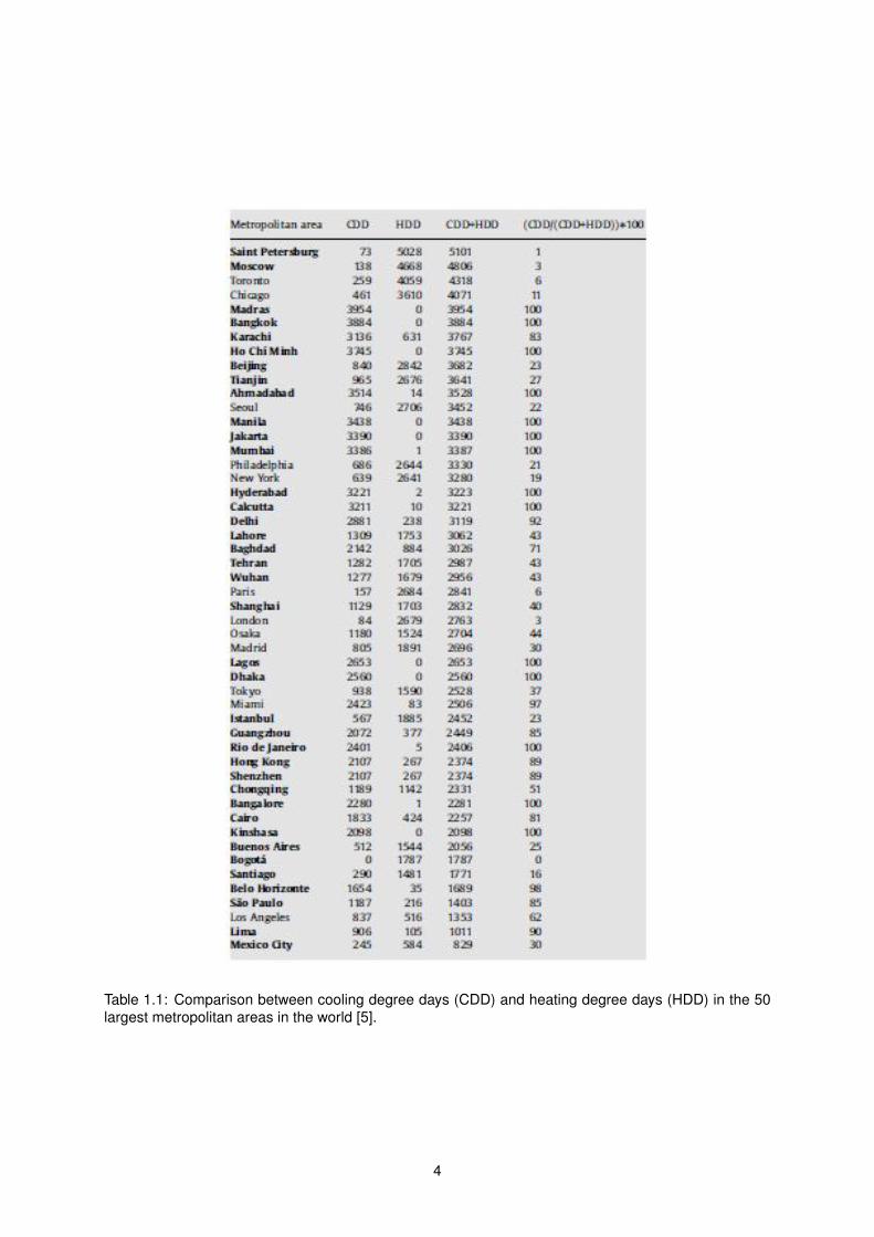
Table 1.1: Comparison between cooling degree days (CDD) and heating degree days (HDD) in the 50largest metropolitan areas in the world [5].
4

of its sound is the low-frequency noise, which also comes from traffic, aircraft and industrial machinery.
Although little research has been done about this subject, it is a dangerous health hazard and it should
be taken seriously, as shown in [6].
1.3 Noise Legislation
Given the hazardous effects of noise, there are laws which define the maximum noise levels allowed in
certain areas and in given periods of time along a 24-hour day, although there are not any international
noise standards defined. Taking as an example the Portuguese Law, the maximum noise values allowed
are presented in Table 1.2. A ”sensitive” zone is defined as a residential, school or hospital area where
Zone Lden(dB(A)) Ln(dB(A))Mixed 65 55Sensitive 55 45Other 63 43
Table 1.2: Maximum noise levels per area in Portuguese territory [7].
normal activities can be easily disturbed by excessive noise whereas a ”mixed” zone is defined as an
area where there are simultaneously industrial or large commercial businesses which have more leeway
for noise and sectors that belong to the sensitive category. Any zone that does not meet any of the
criteria defined above is labeled as ”other”.
Lden is defined as a noise indicator or sound pressure level associated to general nuisance and it is
given by
Lden = 10 log1
24[13× 10
Ld10 + 3× 10
Le+510 + 8× 10
Ln+1010 ] , (1.1)
where Ld, Le and Ln are the daytime, afternoon and night noise indicators.
The country which consumes more energy for air conditioning is the United States, so much that
New York has a specific noise code for air conditioning, where it is stated that a single AC device cannot
produce more than 42 dB(A) measured three feet from the noise source and the cumulative noise level
of multiple devices cannot exceed 45 dB(A) with the same measuring standards as before [8].
There is also specific air conditioning noise legislation in Canada, also a high AC consuming country,
where the noise limits are 45 db(A) and 50 dB(A) for rural and urban areas, respectively. In more noisy
areas such as near railway tracks and highways, there is an exceptional limit of 55 db(A) [9].
1.4 Objectives
The main objective of this work is to minimize the noise produced by an existing air conditioning fan, in
close collaboration with a world leading air conditioning manufacturer, while maximizing its aerodynamic
efficiency by performing an aeroacoustic optimization of the fan blades, with the blade geometry as the
driving design variable.
5

An existing and tested aeroacoustic tool will be adapted to the case in study and used to characterize
the initial fan, in order to have a baseline to compare the final results to.
1.5 Thesis Outline
In Chapter 2, some basic aeroacoustic concepts are defined and an extensive overview of the most rele-
vant noise mechanisms in a fan are presented. The numerical models implemented in the aeroacoustic
tool and used throughout this work to model the noise mechanisms are also introduced, along with the
BEM method to be used for aerodynamic predictions.
In Chapter 3, the characteristics and functioning principles of the custom aeroacoustic tool that will
be used are described. The validation of the tool using known data from a typical axial flow fan is
presented.
In Chapter 4, an overview of the most common airfoil parametrization methods is done and one is
chosen to parametrize the blade airfoils. Also the used 3D parametrization method for building any blade
geometry is described.
In Chapter 5, the baseline fan geometry and the process of inputing it in the aeroacoustic tool is
defined. Also, the baseline noise levels are characterized and the used final method is explained.
In Chapter 6, a parametric study is conducted to evaluate the impact of fan diameter and blade
number on the noise produced.
In Chapter 7, a final aeroacoustic optimization is performed on the baseline fan and on the best case
obtained in chapter 6 and the respective results are presented and discussed.
The thesis ends in Chapter 8 with overall conclusions and remarks and comments on future work.
6

Chapter 2
Fan Aeroacoustics
In this chapter, the concepts of sound and noise are briefly defined and the underlying theory of some
of the noise generation mechanisms of low speed fans is presented, along with how the theory will be
modeled in the noise prediction tool that will be used. A section detailing the method to predict some
aerodynamic parameters is also present.
2.1 Sound and Noise
Sound is a physical phenomena that consists on the propagation of a pressure oscillation through a
given medium, consisting of successive cycles of expansion and contraction of air with changes in air
density related to the pressure change created by the sound source. The intensity and frequency of
these cycles can be sensed and measured in order to characterize the sound, so that sound is modeled
as a wave with a given frequency f and velocity v.
Noise is related to the comfort levels of the human ear. If a given sound becomes annoying or
repetitive in such a way that causes discomfort or impacts the normal functioning of the human being in
its environment, then that sound is defined as noise. Noise is present in most of the everyday appliances
such as computer fans, air conditioning systems and in situations like traffic.
2.2 Sound Pressure Level and Noise Scales
The spectrum of pressure disturbances detectable as sound by the human ear is very wide, therefore it
was required to define a scale that characterizes the intensity of sound within a more practical range of
values.
Knowing that the human perceived intensity is not linear, such that a sound with double the pressure
disturbance will not feel two times more intense, this scale was defined logarithmically and it was named
7

Sound Pressure Level (SPL). SPL is defined by equation (2.1) [10] and it is expressed in decibels (dB)
SPL = 10 log10
(p2rms
p2ref
), (2.1)
where pref is a pressure reference value, usually defined at 2×10⁻⁵ Pa, and p2rms is the sound pressure
root mean square defined by
p2rms = lim
t→∞
1
t
∫ t
0
p2(t)ds . (2.2)
Therefore, from equation (2.1), it is possible to observe that if the intensity of a sound is doubled, its
SPL increases by 3 dB.
In order to make an assessment on typical values in this scale, the sound pressure levels for some
example sounds are presented in table 2.1.
Sound Pressure Level (dB) Sound Examples10 Human breathing (3m away)20 Falling leaf30 Empty cinema room60 Conversation between two people70 Urban traffic80 Vacuum cleaner90 Factory work environment
100 Pneumatic hammer (2m away)110 Motorcycle engine revving(5m away)120 Rock concert130 Pain threshold140 Jet engine (3m away)
Table 2.1: Examples of sounds and their respective SPL [10].
The Sound Pressure Level quantifies objectively the intensity of a sound, but it does not account for
the impact of sound frequency in its perception by the human ear. A 100 Hz sound will be perceived
with an intensity level 20 dB lower than its original intensity level while the perceived intensity of a 1000
Hz sound will remain the same. To account for this effect, the A-,B- and C-weightings were created in
order to correct the original SPL scale and to have an objective way to measure how tones of sounds
with the same intensity are perceived differently. The relation between the sound frequency and the
change in intensity is shown in figure 2.1. The A-weighting is the most commonly used, being suited for
low to medium levels, while the B- and C-weighting are used more for higher intensity levels. When the
A-weighting correction is applied, the sound pressure level is measured in dB(A).
2.3 Tonal and Broadband Noise
In common knowledge, it is usual to associate high frequency sound to high pitched tones, such as a
whistle and low frequency sound to low pitched tones, such as a drum beat. Although this association
is not wrong, it is only completely true for a pure tone, which is a sound consisting in a pure sinusoidal
wave with a fixed frequency.
8

Figure 2.1: Representation of the different noise scale corrections.
Pure tones are produced only artificially by electronic oscillators and do not exist in Nature. In reality,
all the sounds that we know are a complex combination of sound components of various frequencies
and intensities which compose what is known as the sound spectrum. An example of a spectrum is
shown in figure 2.2. It is common to define the range for the frequency axis in a spectrum plot between
100 Hz and 16∼17 kHz, since the spectrum of human audible frequencies is comprised between 20
Hz and 20 kHz, but as it can be seen in figure 2.1 considering A-weighting, the ear is less sensitive to
sounds with frequency less than 100 Hz and higher than 12 kHz.
After a sound spectrum is obtained, there may exist some spikes in certain frequency bands that
stand out from the rest of the spectrum. These spikes are referred to as tonal noise (or narrow band
noise) and if they have fundamental high relative amplitude, the overall noise may be dominated by tonal
noises. In most cases, tonal noises are harmonic, consisting of a fundamental frequency f , which is the
frequency where the first spike is detected, plus the harmonics are multiples of f usually with smaller
amplitude than the fundamental, but nonetheless higher when compared to the rest of the spectrum, in
frequencies of 2f ,3f , etc.
What until now has been referred as the rest of the spectrum, is called broadband noise, because
it is not defined in a single frequency band like tonal noise, being instead a distributed noise along the
frequency spectrum. Good examples for broadband noise are the wind noise, traffic noise or any kind of
background noise. The distinction between tonal and broadband noise is also represented in figure 2.2.
2.4 Fan Noise Mechanisms
The two major sources of noise in a low speed fan, as with any other fan, are mechanical and aeroa-
coustic sources, as shown in figure 2.3.
9

Figure 2.2: Frequency spectrum of a sound [11].
2.4.1 Mechanical Noise
As with any mechanical system with moving parts, the dynamic interaction between each component
creates noise. In an air conditioning system, this noise derives mainly from the engine and driver belts
responsible for the motion of the fan and also from the compressor [12].
Despite these sources, modern systems have very efficient noise reduction techniques and with
modern manufacturing materials and technology, mechanical noise in fans is just a small fraction of the
total noise.
2.4.2 Aeroacoustic Noise
Aeroacoustic noise is the major source for the total noise of a low speed fan, with the fan geometry (e.g.
airfoils and blade twist) as the main design driver which has an impact on reducing this type of noise.
Aeroacoustic noise in fans can be divided in three groups: low frequency noise, turbulent inflow noise
and airfoil self-noise.
Low frequency noise is related to the Blade Passing Frequency or BPF of the fan, which will be
defined later in this section. Turbulent inflow noise is created when there is an interaction between the
airfoil and the incoming turbulent flow and airfoil self-noise is a consequence of the interaction between
the self-produced boundary layer and wake and the airfoil itself. There are five known self-noise mecha-
nisms which are Trailing Edge Bluntness Vortex Shedding (TEB-VS), Tip Vortex Formation (TVF), Sep-
aration/Stall, Laminar Boundary Layer Vortex Shedding (LBL-VS) and Turbulent Boundary Layer Trailing
Edge (TBL-TE).
Low Frequency Noise
Whenever a rotating body, such as the blade of a fan, rotates at a constant angular velocity in an air
flow, it experiences aerodynamic forces. In turn, the reaction forces from the rotating body accelerate
10

Fan Noise
Mechanisms
Mechanical Noise Aeroacoustic Noise
Low Frequency
Noise
Turbulent Inflow
NoiseAirfoil Self-Noise
Laminar Boundary
Layer Vortex
Shedding Noise
Turbulent Boundary
Layer Vortex
Shedding Noise
Separation/Stall
Noise
Tip Vortex
Formation Noise
Trailing Edge
Bluntness Vortex
Shedding Noise
Figure 2.3: Fan noise sources.
the surrounding air, which generates pressure disturbances and therefore produces sound [13].
If a fixed point in space is considered, the sound produced by a rotating blade can be thought out
as an impulse in the air located in that point, whenever the blade passes through that point. So, if the
number of times a blade passes through a given point is increased, the impulses and the produced
sound also increases, being generated a sound wave with a frequency equal to the number of impulses
created in a second.
In a fan or any rotor-like mechanism, this phenomena is characterized by the Blade Passing Fre-
quency (BPF) which translates the amount of times that all the blades pass through a generic point in a
second, such that a fan with an high rotating speed and number of blades will have an high BPF. BPF is
given by
BPF =NZ
60, (2.3)
with N as the fan rotating speed in RPM and Z as the number of blades.
For low speed fans, this frequency is usually very low, between 40 and 100 Hz, due to the low rotating
speed which turns the BPF noise or low frequency noise, in this case, almost inaudible due to belonging
in the low end of the human audible frequency spectrum. Therefore, although it is a tonal noise, low
frequency noise in low speed fans becomes almost irrelevant.
Trailing Edge Bluntness Vortex Shedding Noise
Although the trailing edge of an airfoil is idealized as being just a point where the pressure and suction
surfaces connect in the rear end, in reality there is always an edge with finite thickness in the end of the
airfoil, due to manufacturing constraints.
11

This trailing edge with thickness creates a coherent vortex shedding, also known as a Von Karman
vortex sheet [14], due to the differential of pressure between the two surfaces of the airfoil. As these
vortexes are shed, a varying pressure fluctuation is generated along the trailing edge, producing a
radiating noise of tonal nature of varying discrete frequencies, which is called Trailing Edge Bluntness
Vortex Shedding noise.
The noise produced by this mechanism is correlated to the trailing edge thickness and angle, being
extremely sensitive to changes in any of these variables, such that one effective method of reducing this
noise is to minimize the thickness and smooth the trailing edge angle as physically possible. However, it
is important to notice that any change in the trailing edge will affect the lift produced by the airfoil, since
a variation on the trailing edge thickness will impact the circulation that relates to the lift as
L = −ρUΓ , (2.4)
where ρ is the air density, U is the air speed and Γ is the attached circulation in the airfoil. Therefore,
there is a compromise to be had between the reduction of the noise produced by this mechanism and
the impact in the overall lift. A schematic representation of this phenomenon is presented in figure 2.4.
Figure 2.4: Trailing edge bluntness noise [15].
Tip Vortex Formation Noise
In a way analogous to the Trailing Edge Bluntness noise, Tip Vortex Formation noise is a consequence
of the shedding of vortexes in the tip of the blade due to the pressure difference between the upper and
lower surfaces. The interaction between these vortexes and the blade tip produces a pressure fluctuation
which radiates a broadband noise [15]. This noise mechanism is highly sensitive to the topology of the
tip geometry. A schematic representation of this noise producing mechanism is presented in figure 2.5.
Figure 2.5: Tip vortex noise [15].
12

Separation/Stall Noise
When the angle of attack of an airfoil is very high, the flow separates from the suction surface, creating
a zone with highly recirculating and unsteady flow containing turbulent eddies. When these eddies
interact with the airfoil wake, a broadband noise is produced with the name of Separated Stall noise
[15]. A schematic representation of this noise producing mechanism is presented in figure 2.6.
Figure 2.6: Separation/stall noise [15].
Laminar Boundary Layer Vortex Shedding Noise
Any airfoil subject to a flow will develop a boundary layer in all of the extent of its surface between the
leading and the trailing edge, which for low Reynolds number and angles of attack, is denominated as a
laminar boundary layer.
This boundary layer is created due to the existence of an adverse pressure gradient that is found
along the airfoil surfaces in the streamwise direction, which creates pressure instabilities along the layer.
When these instabilities interact with the vortexes shed by the trailing edge, a sound is radiated
from the TE, being defined as the Laminar Boundary Layer Vortex Shedding Noise [15]. A schematic
representation of this noise is presented in figure 2.7.
Figure 2.7: Laminar boundary layer vortex shedding noise [15].
13

Figure 2.8: Turbulent boundary layer trailing edge noise [15].
Turbulent Boundary Layer Trailing Edge
If certain conditions are met such as an high Reynolds number and a given angle of attack, the existing
boundary layer in the airfoil will transition from laminar to turbulent at a given chordwise position.
In a turbulent boundary layer, there is an high recirculation of flow which induces a pressure fluctu-
ation zone and analogously to LBL-VS noise, when these fluctuations interact with the vortexes shed
by the trailing edge, a broadband noise is emitted. This noise is named as Turbulent Boundary Layer
Trailing Edge Noise [15] and it is depicted schematically in figure 2.8.
Turbulent Inflow Noise
In most industrial fan applications, it is rarely found a situation where the inflow that goes through the
fan is perfectly uniform, most often including sheared flow with different velocity profiles which creates
turbulent eddies of various sizes and speeds.
In the specific case of outdoor air conditioning units, the turbulent inflow is mainly a consequence of
the inlet and its geometrical characteristics (e.g open versus grid inlet), and when the turbulent inflow
encounters the fan, it produces a broadband, vibrating sound which is called the Turbulent Inflow Noise
[15].
This noise is characterized by two quantities; the turbulence intensity, which is a numerical indicator
of the turbulence fluctuations and it is defined as the ratio between the eddies velocity standard deviation
and the mean flow speed, and the turbulence length scale, which is the characteristic dimension related
to the eddies size.
While it is a broadband noise, there is a correlation between the frequency of the noise produced
and the size of the eddies. If the eddies are large, they will affect the airfoil and change its response
as a whole, therefore producing low frequency noise. If the eddies are small, it will produce a localized
response which will radiate an high frequency noise [15].
2.5 Noise Prediction Method
The method used in this work to predict the fan noise consists in dividing the blades into segments with
a given span length, measured radially and defined by the airfoil shapes where the blade is sectioned.
Given these segments, the numerical noise prediction models are then applied to the airfoil shapes,
since in the 2D approximation presented in [16], the noise radiated by a blade segment can be assumed
to be similar to the noise radiated by an equivalent airfoil section. This approximation is valid assuming
14

that the blade elements are not too close the hub and tip areas. For the elements that have proximity to
these zones, a hub and tip correction is applied and it will be presented in Section 2.6.1.
Therefore, assuming mutually incoherent radiation from the blades [17], the sound pressure level of
each blade segment can be computed and the total sound power level of the rotor for each frequency
band is the sum of the noise produced by each noise element, given by
Lip,total = 10 log10
NBNaz
∑j
10
Lip,j10
, (2.5)
where NB is the number of blades of the fan, Naz is the number of azimuthal positions where the blade
is sectioned and Lip,j is the sound power level computed in the j blade segment for the i frequency band.
With the sound power level computed for a spectrum of frequency bands, it is possible to calculate
the total sound power level for the fan by adding the SPL for each frequency band,
Lp,overall = 10 log10
∑i
10
Lip,total10
, (2.6)
being the sum defined as the Overall Sound Pressure Level (OASPL).
In order to compute the noise produced by each blade segment, a numerical noise prediction model
or set of models has to be chosen, considering the objectives of the work and the required level of
accuracy. In Computational Aeroacoustics, noise prediction numerical schemes for axial flow fans can
be classified in the following way:
• Class I methods Predictions giving an estimate of overall noise level as a simple algebraic
function of basic machine parameters, such as, diameter, speed, flow rate, among others;
• Class II methods Predictions based on separate consideration of the various mechanisms caus-
ing fan noise, using selected fan parameters, being required some assumptions to simplify the
problem;
• Class III methods Predictions using full information about the noise mechanisms requiring a
detailed description of geometry and aerodynamics, being necessary the use of an advanced
CFD tool.
While Class III methods are those that produce the most accurate results, they are very resource-
intensive and time-consuming and are not suited for the preliminary design phase of a fan, being com-
monly used by academic researchers. Class I methods are very fast, but exceedingly simple with a risk
to over or under-predict the noise levels with an high error level. Therefore, for the sake of compromise
between speed and accuracy, the best choice for this work are Class II methods.
These methods consist mainly in semi-empirical schemes, which are a set of formulas determined
by coupling analytic analysis and experimental data, by fitting the data into an expression which allows
for a quick and simple replication of that data through the input of some selected parameters.
15

In order for these schemes to maintain their simplicity, some assumptions and simplifications have
to made, such as acoustic compactness, which means that the dimensions of the noise sources, which
in this case is the chord and span length of the blade segments, have to be smaller that the wavelength
of the sound emitted. So, the higher the frequency for which it is desired that the methods are valid, the
smaller the blade segments have to be. For example, in order for a calculation for 10 kHz to be valid, the
chord and span length of a blade segment cannot exceed 3.4 centimeters.
Another simplification is to assume that the flow is mainly two dimensional, since most of the pre-
sented semi-empirical methods in this section, are applicable to airfoil in two dimensional flows. This
is largely true for outboard, but not too close to the hub and tip area, blade sections, which tend to
dominate the noise production. Additionally, in [18] it is argued that the sound spectrum of a rotating
broadband source is not strongly affected by its rotation, if the angular velocity is low enough, which
means, for noise prediction purposes, that stationary, single surface, two dimensional methods can be
applied to a rotating fan.
Despite these assumptions, the accuracy of these prediction schemes is satisfactory, considering
the low amount of resources and time required for the computation of the prediction, being suited to use
in an optimization procedure, which requires a fast and simple calculation method in order to be used in
a high number of iterations in a short time.
2.5.1 TEB-VS Noise Prediction Model
Brooks and Marcolini [15] derived a formula from experimental data obtained by Brooks and Hodgson
[19] to predict Trailing Edge Bluntness noise,
LBlunt = 10 log
(hM5.5LDh
r2e
)+G1
(h
δ∗avg,Ψ
)+G2
(h
δ∗avg,Ψ,
St′′′
St′′′peak
), (2.7)
where h is the bluntness thickness, M is the airfoil local Mach number, L is the blade element length, re
is the effective observer distance, Dh is a directivity function which is defined in Subsection 2.5.7, δ∗avg
is the average between the pressure and suction surfaces boundary layer displacement thicknesses,
(δ∗p + δ∗s )/2 and Ψ is the trailing edge angle.
The characteristic length used to define the Strouhal number St′′′
is the trailing edge thickness,
St′′′
=fh
U, (2.8)
with f as the frequency for which the noise is computed and U as the mean flow velocity.
The peak Strouhal number is defined by the following relations:
St′′′
peak =
0.212− 0.0045Ψ
1 + 0.235 (h/δ∗avg)−1 − 0.0132 (h/δ∗avg)
−2 (h/δ∗avg ≥ 0.2)
0.1 (h/δ∗avg) + 0.095− 0.00243Ψ (h/δ∗avg < 0.2)
(2.9)
The function G1 determines the peak level of the spectrum and it is a function of the thickness ratio
16

and trailing edge angle,
G1
(h
δ∗avg,Ψ
)=
17.5 log (h/δ∗avg) + 157.5− 1.114Ψ (h/δ∗avg ≤ 5)
169.7− 1.114Ψ (h/δ∗avg > 5), (2.10)
and the spectral shape function G2 involves an interpolation between angles Ψ = 14 and Ψ = 0 ,
G2
(h
δ∗avg,Ψ,
St′′′
St′′′peak
)= (G2)Ψ=0 + 0.0714Ψ [(G2)Ψ=14 − (G2)Ψ=0 ] . (2.11)
Due to being overly extensive, functions (G2)Ψ=14 and (G2)Ψ=0 are presented in Appendix A.1.
2.5.2 Tip Vortex Formation Noise Prediction Model
The prediction for Tip Vortex noise is given by the following formula, defined by Brooks [15]:
LTip = 10 log
(M2M3
max`2Dh
r2e
)− 30.5 (logSt′′ + 0.3)
2+ 126 , (2.12)
where ` is the spanwise extent of the separation caused by the tip vortex at the trailing edge.
The Strouhal number is
St′′ =f`
Umax. (2.13)
In the case of a rounded tip, ` can be estimated by
`
c≈ 0.008αTIP , (2.14)
where αTIP is the angle of attack of the tip of the blade. For the case of a flat tip,
`/c =
0.0230 + 0.0169α′TIP (0 ≤ α′TIP ≤ 2 )
0.0378 + 0.0095α′TIP (2 < α′TIP )
, (2.15)
with α′TIP given by
α′TIP =
[(∂L′/∂y
(∂L′/∂y)ref
)y→TIP
]αTIP . (2.16)
The maximum Mach number Mmax of the flow within or about the separated flow region at the trailing
edge and the respective maximum speed Umax are
Mmax/M ≈ (1 + 0.036αTIP ) (2.17a)
and
Umax = c0Mmax (2.17b)
A representation of some of the referred variables above is shown in figure 2.9.
17

Figure 2.9: Variables used in tip vortex noise prediction [15].
2.5.3 LBL-VS Noise Prediction Model
The proposed model for prediction of Laminar Boundary Layer Vortex Shedding Noise, defined by
Brooks and Hodgson [19], is described by,
LLBL−V S = 10 log
(δpM
5LDh
r2e
)+G3
(St′
St′peak
)+G4
[Rc
(Rc)0
]+G5(α∗) , (2.18)
where δp is the boundary layer thickness in the pressure side, G3, G4 and G5 are spectral functions
which are defined in Appendix A.2, Rc is the chordwise Reynolds number and α∗ is the local effective
angle of attack.
The Strouhal number St′ is defined as
St′ =fδpU
(2.19)
and
St′1 =
0.18
(Rc ≤ 1.3× 10⁵
)0.001756R0.3931
c
(1.3× 10⁵ < Rc ≤ 4× 10⁵
)0.28
(4× 10⁵ < Rc
) , (2.20)
with
St′peak = St′1 × 10−0.04α∗ . (2.21)
18

2.5.4 TBL-TE Noise Prediction Model
The scaling effort done by Brooks and Hodgson[15], based on the work from Ffowcs Williams and Hall
[20] in order to predict Turbulent Boundary Layer Trailing Edge Noise results in,
LTBL−TE = 10 log(
10Lα/10 + 10
Ls/10 + 10Lp/10
), (2.22)
where Lα, Ls and Lp are the sound pressure levels for each contribution.
The pressure side contribution is given by
Lp = 10 log
(δ∗pM
5LDh
r2e
)+A
(StpSt1
)+ (K1 − 3) + ∆K1 , (2.23)
the suction side by
Ls = 10 log
(δ∗sM
5LDh
r2e
)+A
(StsSt1
)+ (K1 − 3) (2.24)
and separation/stall by
Lα = 10 log
(δ∗sM
5LDh
r2e
)+B
(StsSt2
)+K2 , (2.25)
where δ∗ is the boundary layer displacement thickness and A, B, K1 and K2 are empirical spectral
shape and amplitude functions described in Appendix A.3.
Since most of the models developed by Brooks and Hodgson are based on the NACA 0012 airfoil,
they defined that for angles of attack higher than 12.5 , which is stall angle for the same airfoil, the
TBL-TE noise mechanism consists mainly in the separation/stall contribution, being the equations (2.23)
to (2.25) replaced by
Lp = −∞ , (2.26)
Ls = −∞ (2.27)
and
Lα = 10 log
(δ∗sM
5LD`
r2e
)+A′
(StsSt2
)+K2 , (2.28)
where A′ is the shape function A for a Reynolds number three times the actual Reynolds number.
The Strouhal numbers are defined by these set of equations:
Stp =fδ∗pU
, (2.29)
Sts =fδ∗sU
, (2.30)
St1 = 0.02M−0.6 (2.31)
19

and
St2 = St1 ×
1 (α∗ < 1.33)
100.0054(α∗−1.33)2 (1.33 ≤ α∗ ≤ 12.5)
4.72 (α∗ > 12.5)
. (2.32)
2.5.5 Turbulent Inflow Noise Prediction Model
For the prediction of Turbulent Inflow Noise, a semi-empirical method developed by Carolus and Schnei-
der in [21] specifically for axial flow fans was chosen.
The basis of this method consists on the prediction of the spectral density of the acoustic power W
radiated from Z uncorrelated broadband sources, which in this work will be considered as the number
of blades, and it is given by
PSDW (f) ≡ dW (f)
df=π
4
Z
ρc20
f
ra(1− (ri/ra)2)2ΨPSDF (f) , (2.33)
where ri is the hub radius, ra =D
2, D is the diameter of the fan, ρ is the fluid density (in this case, air)
and c0 is the speed of sound. The radiation factor Ψ accounts for mean flow in both the +x and −x
directions, but due to the case in study being a low axial flow Mach number, this factor is set to 1.
In this model, the aeroacoustic sources are represented by the force fluctuation on a blade, PSDF ,
which can be expressed in terms of the fluctuating surface pressure distribution, PSDsp, and the corre-
lation area Ac, as
PSDF (f) =
∫∫A
PSDsp(f, ξ1, ξ3)Ac(f, ξ1, ξ3)dξ1dξ3 . (2.34)
In this work, equation (2.34) is approximated by using the blade division which was described in
the beginning of Section 2.5 and evaluating and summing the product between the integrand and the
projected area of each blade segment. This projected area is calculated using a numerical integration
scheme, more specifically, the Simpson’s rule.
The coordinates ξ1 and ξ3 are part of the rotating frame of reference defined in the model which is
shown in figure 2.10, along with the used stationary coordinate system.
As it was previously referred, this noise mechanism is due to the turbulent eddies approaching the fan
which cause a fluctuating pressure difference between the two sides of a blade. This fluctuation is due
to an imposing and varying velocity, consequence of the eddies turbulence, w′2 which is perpendicular
to the blade surface and w′2 w1, with w1 as the local speed of the blade segment in the rotating frame
of reference.
Defining the spectral density of the imposed velocity fluctuation as PSDw2 ≡dw′2df
, the desired
fluctuating pressure distribution PSDsp will be given by
PSDsp ≡d∆p′2
df=
1
4(0.9π)2ρ2w2
1PSDw2 . (2.35)
For small angles γ, PSDw2 can be approximated by the one-dimensional energy spectrum PSDcx ≡
20
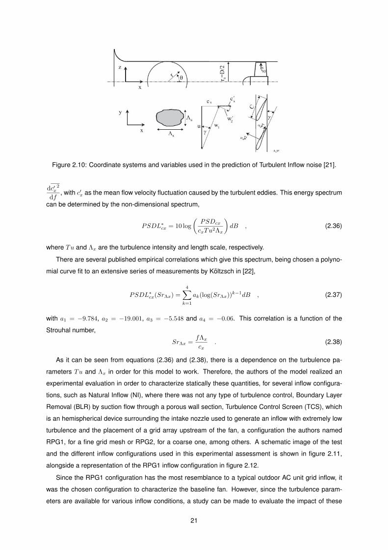
Figure 2.10: Coordinate systems and variables used in the prediction of Turbulent Inflow noise [21].
dc′x2
df, with c′x as the mean flow velocity fluctuation caused by the turbulent eddies. This energy spectrum
can be determined by the non-dimensional spectrum,
PSDL∗cx = 10 log
(PSDcx
cxTu2Λx
)dB , (2.36)
where Tu and Λx are the turbulence intensity and length scale, respectively.
There are several published empirical correlations which give this spectrum, being chosen a polyno-
mial curve fit to an extensive series of measurements by Koltzsch in [22],
PSDL∗cx(SrΛx) =
4∑k=1
ak(log(SrΛx))k−1dB , (2.37)
with a1 = −9.784, a2 = −19.001, a3 = −5.548 and a4 = −0.06. This correlation is a function of the
Strouhal number,
SrΛx =fΛxcx
. (2.38)
As it can be seen from equations (2.36) and (2.38), there is a dependence on the turbulence pa-
rameters Tu and Λx in order for this model to work. Therefore, the authors of the model realized an
experimental evaluation in order to characterize statically these quantities, for several inflow configura-
tions, such as Natural Inflow (NI), where there was not any type of turbulence control, Boundary Layer
Removal (BLR) by suction flow through a porous wall section, Turbulence Control Screen (TCS), which
is an hemispherical device surrounding the intake nozzle used to generate an inflow with extremely low
turbulence and the placement of a grid array upstream of the fan, a configuration the authors named
RPG1, for a fine grid mesh or RPG2, for a coarse one, among others. A schematic image of the test
and the different inflow configurations used in this experimental assessment is shown in figure 2.11,
alongside a representation of the RPG1 inflow configuration in figure 2.12.
Since the RPG1 configuration has the most resemblance to a typical outdoor AC unit grid inflow, it
was the chosen configuration to characterize the baseline fan. However, since the turbulence param-
eters are available for various inflow conditions, a study can be made to evaluate the impact of these
21
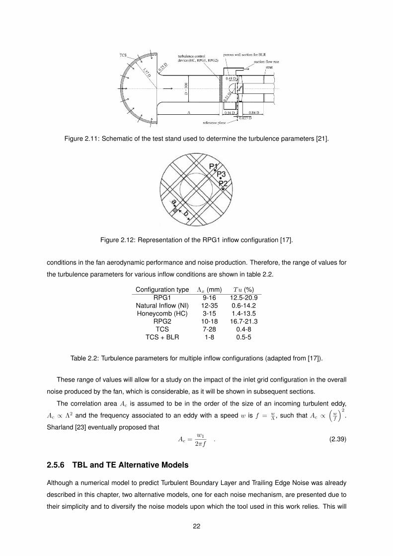
Figure 2.11: Schematic of the test stand used to determine the turbulence parameters [21].
Figure 2.12: Representation of the RPG1 inflow configuration [17].
conditions in the fan aerodynamic performance and noise production. Therefore, the range of values for
the turbulence parameters for various inflow conditions are shown in table 2.2.
Configuration type Λx (mm) Tu (%)RPG1 9-16 12.5-20.9
Natural Inflow (NI) 12-35 0.6-14.2Honeycomb (HC) 3-15 1.4-13.5
RPG2 10-18 16.7-21.3TCS 7-28 0.4-8
TCS + BLR 1-8 0.5-5
Table 2.2: Turbulence parameters for multiple inflow configurations (adapted from [17]).
These range of values will allow for a study on the impact of the inlet grid configuration in the overall
noise produced by the fan, which is considerable, as it will be shown in subsequent sections.
The correlation area Ac is assumed to be in the order of the size of an incoming turbulent eddy,
Ac ∝ Λ2 and the frequency associated to an eddy with a speed w is f = wΛ , such that Ac ∝
(wf
)2
.
Sharland [23] eventually proposed that
Ac =w1
2πf. (2.39)
2.5.6 TBL and TE Alternative Models
Although a numerical model to predict Turbulent Boundary Layer and Trailing Edge Noise was already
described in this chapter, two alternative models, one for each noise mechanism, are presented due to
their simplicity and to diversify the noise models upon which the tool used in this work relies. This will
22
allow the fine tuning of the tool for the characterization of the baseline fan.
These models have the same basis as the Turbulent Inflow Noise prediction model, such that equa-
tions (2.33) and (2.34) also apply, with the difference residing in the computation of the PSDsp and Ac
terms.
Turbulent Boundary Layer Noise Model
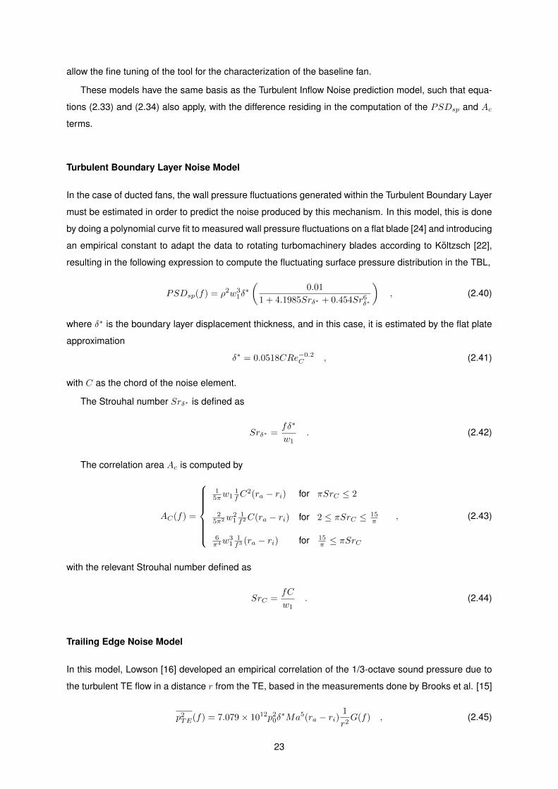
In the case of ducted fans, the wall pressure fluctuations generated within the Turbulent Boundary Layer
must be estimated in order to predict the noise produced by this mechanism. In this model, this is done
by doing a polynomial curve fit to measured wall pressure fluctuations on a flat blade [24] and introducing
an empirical constant to adapt the data to rotating turbomachinery blades according to Koltzsch [22],
resulting in the following expression to compute the fluctuating surface pressure distribution in the TBL,
PSDsp(f) = ρ2w31δ∗(
0.01
1 + 4.1985Srδ∗ + 0.454Sr6δ∗
), (2.40)
where δ∗ is the boundary layer displacement thickness, and in this case, it is estimated by the flat plate
approximation
δ∗ = 0.0518CRe−0.2C , (2.41)
with C as the chord of the noise element.
The Strouhal number Srδ∗ is defined as
Srδ∗ =fδ∗
w1. (2.42)
The correlation area Ac is computed by
AC(f) =
15πw1
1fC
2(ra − ri) for πSrC ≤ 2
25π2w
21
1f2C(ra − ri) for 2 ≤ πSrC ≤ 15
π
6π4w
31
1f3 (ra − ri) for 15
π ≤ πSrC
, (2.43)
with the relevant Strouhal number defined as
SrC =fC
w1. (2.44)
Trailing Edge Noise Model
In this model, Lowson [16] developed an empirical correlation of the 1/3-octave sound pressure due to
the turbulent TE flow in a distance r from the TE, based in the measurements done by Brooks et al. [15]
p2TE(f) = 7.079× 10¹²p2
0δ∗Ma5(ra − ri)
1
r2G(f) , (2.45)
23

Figure 2.13: Angles used in sound directivity functions.
with p0 as a reference pressure of 2 × 10⁻⁵ Pa, Ma is the tip Mach number and the spectrum shape
function G(f) given by
G(f) =4(f/fpeak)2.5
(1 + (f/fpeak)2.5)2(2.46)
and the peak frequency
fpeak =0.02w1Ma−0.6
δ∗. (2.47)
If the sound power is integrated as if the sound is radiated from the trailing edge as a spherical wave,
the total Sound Power Spectral Density of trailing edge noise is given by
PSDTE(f) = 7.079× 10¹²P0δ∗Ma5(ra − ri)
4π
∆f1/3octG(f) , (2.48)
where P0 is the reference sound power, 10−12 W and ∆f1/3oct is the bandwidth of each 1/3-octave band.
To calculate the sound power produced by this mechanism of the complete fan, equation (2.48) must
be multiplied by the number of blades. The result of this computation will be added to the one obtained
from equation (2.33) in order to have the sum of the contributions of all the noise mechanisms to which
the equation applies.
2.5.7 Directivity Functions
Following the work of Amiet [25], Brooks and Hodgson [15] presented the directivity functions for high
and low frequencies, which are functions that take into account the relative perception of different noise
mechanisms from different points in the airfoil by the observer in its position. These functions are nor-
malized by the trailing edge noise emitted in the Θe = 90 and Φe = 90 direction, which means that
Dh(90 , 90 ) = 1, meaning that sound directivity reaches its maximum in the TE. The angles Θe and Φe
are defined in figure 2.13.
For high frequencies, the directivity is given by
Dh(Θe,Ψe) ≈2 sin2(Θe/2) sin2 Φe
(1 +M cos Θe)[1 + (M −Mc) cos Θe]2, (2.49)
24

(a) (b)
Figure 2.14: Set of coordinate systems.
where Mc ≈ 0.8M . For low frequencies, the directivity is given by
D`(Θe,Ψe) ≈sin2 Θe sin2 Ψe
(1 +M cos Θe)4. (2.50)
When an airfoil is fixed in space, relatively to the observer, the computation of the directivity becomes
a simple task, since the angles and distances are constant and easily calculated. But when trying to
predict the noise of a fan, the blade rotation causes additional complications, since the observer does
not follow it, being necessary to perform extra calculations to obtain the angles Θe and Ψe and observer
distance re, used in most of the models described in this section.
In order to solve this problem, a set of coordinate systems needs to be defined. The first coordinate
system (system 1) is placed on the ground, where the observer is standing. System 2 is non-rotating
and its z-axis is aligned with the rotation axis of the fan. System 3 is attached to the rotating shaft and
rotates along with the shaft and it is aligned with one the blades and system 4 is system 3 rotated about
its x-axis with origin in the hub, in order to account for the blade twist.
This approach was originally used for a wind turbine and it is here adapted to the present case. In
figure 2.14a, the referred systems are shown for a wind turbine, but by setting θtilt and θcone equal to
0 and interpreting the wind turbine tower as just the height where the axial fan is installed, the systems
are valid for an axial fan case. In Appendix B, the transformation matrices between the various systems
are defined.
With these systems defined, any point in the blades can be described by a vector r which is obtained
by a sum of vectors, as shown in figure 2.14b,
r = r1 + r2 + r3 . (2.51)
25

Having the vector r defined, the directivity angles Θe and Ψe can be computed as shown in figure
2.13.
2.5.8 Boundary Layer Parameters
With the exception of the TBL-TE noise model, all of the numerical models used in this work to predict the
several noise mechanisms need boundary layer parameters as input. While the authors of those models
provided correlations to compute these parameters, they were determined based on experimental results
from the NACA 0012 airfoil, and therefore are not suited for more general airfoil, such as cambered ones.
Therefore, the noise prediction method in this work is complemented with an external calculation of
the boundary layer parameters using the XFOIL code [26] or the RFOIL code [27].
One shortcoming when using XFOIL is that the code does not compute the boundary layer thickness
δ, being necessary the use of the relation given by Drela and Giles [28],
δ = θ
(3.15 +
1.72
Hk − 1
)+ δ∗ , (2.52)
with θ being the boundary layer momentum thickness and the definition of Hk from [29] for adiabatic flow
in air,
Hk =H − 0.290M2
1 + 0.113M2, (2.53)
where H is the boundary layer shape factor.
2.6 Blade Element Momentum Theory
All of the models presented in this chapter require some aerodynamic parameters as input, such as local
angles of attack or relative velocities and in order to estimate the aerodynamic performance of a fan, a
prediction method is chosen.
While a full Computational Fluid Dynamics simulation using the Navier-Stokes equations would pro-
vide the referred input, it is computationally expensive and complex. Therefore, the Blade Element
Momentum method is chosen for its simplicity, speed and for being the most widely used theory in rotor
preliminary design.
Although the BEM method is frequently used for wind turbine applications [30] [31], it is equally
valid to apply it in axial fans and propellers. Since the underlying theory for this method is extensively
described by many authors [32] [33] [34], only a summarized version will be presented in here.
This method consists in equalizing the thrust and torque relations given by the blade element theory
and the momentum theory, in order to achieve a mathematical expression that models the axial and
tangential induction factors, a and a′ given by
a =u
Vand a′ =
u′
ωr(2.54)
where u is the axial induced velocity, u′ is the radial induced velocity, V is the mean flow speed, ω is the
26

Figure 2.15: Velocities and angles in the rotor plane.
rotational speed of the fan, in radians per second and r is the radial distance of the element where the
method is being applied.
As it can be seen from figure 2.15, the axial induced velocity increases the total axial speed by a
factor of aV and the radial induced velocity decreases the total radial speed by a factor of a′ωr, thus
specifying the axial and radial components of the relative velocity U given by V (1 + a) and ωr(1 − a′),
respectively. Therefore, it can be stated that
tanφ =V (1 + a)
ωr(1− a′), (2.55)
where φ is the inflow angle, the angle between the relative velocity and the rotor plane.
The momentum theory states that for a rotor annulus with a width dr and in the radial location r, the
thrust produced is
dT = 4πrρV 2(1 + a)aFdr , (2.56)
while the torque produced is given by
dQ = 4πr3ρV (1 + a)a′ωFdr , (2.57)
where F is a factor taking into account the hub and tip losses, which will be explained in Section 2.6.1.
The same thrust and torque for the same rotor annulus is also predicted by the blade element theory,
using
dT =1
2ρNB
V 2(1 + a)2
sin2 φcCndr (2.58)
and
dQ =1
2ρNB
V (1 + a)ωr(1− a′)sinφ cosφ
cCtrdr , (2.59)
where NB is the number of blades, c is the element chord and Cn and Ct are, respectively, the coeffi-
cients of the resulting aerodynamic forces in the normal and tangent direction with respect to the rotor
plane and are given by
Cn = Cl cosφ− Cd sinφ (2.60)
27

and
Ct = Cl sinφ+ Cd cosφ . (2.61)
The aerodynamic coefficients Cl and Cd are usually read from an aerodynamic table, or in the case
of this work, aerodynamic polars obtained by computer simulations can be used. The quality of results
produced by the BEM method is very sensitive to the quality of the input aerodynamic data.
By equating equation (2.56) and equation (2.58), the expression for the axial induction factor can be
found as
a =1
4F sin2 φσCn
− 1, (2.62)
where σ = c(r)NB2πr is the local solidity. If the same procedure is done for equations (2.57) and (2.59), the
radial induction factor is given by
a′ =1
4F sinφ cosφσCt
+ 1. (2.63)
2.6.1 BEM Corrections
Tip Loss
In the original BEM theory, the losses due to the effect of blade tip vortex shedding in the induced velocity
field were not accounted for. Therefore, Prandtl [35] [36] defined a loss factor to correct the BEM theory
as
F =2
πcos−1(e−f ) , (2.64)
where
f =NB2
R− rr sinφ
(2.65)
and R is the blade radius.
Hub Loss
Since there are also vortexes that are shed near the hub, a correction factor for the hub can also be
derived. This factor is computed by the same procedure that the tip loss factor, with the exception of
replacing the equation (2.65) by
f =NB2
r −Rhubr sinφ
. (2.66)
With these two loss factors computed, the total loss factor to be used is given by their product,
F = FtipFhub . (2.67)
2.6.2 Fan Efficiency
The main task of an axial flow fan is to push the most volume of air possible while using the least amount
of energy to support its rotation. The power imparted by the fan to the flow can be expressed by the
28

Figure 2.16: Actuator disk (propeller).
product of the total pressure rise through the fan with the volumetric flow rate delivered by the fan, ∆pq.
This pressure rise can be explained by the fact that the fan accelerates the flow while it passes from
the back to the front of the fan, so that the number of air particles is higher in the front that in the back.
That will create a pressure rise between the both sides of the fan.
The basic aerodynamic principles of the axial fan, which in theory can be idealized as propeller disk,
can be described the actuator disk concept, represented in figure 2.16. If the fan is modeled as a uniform
disk with infinite blades, the pressure rise P2 − P1 can be thought of as a reaction force applied in the
fan, or in other words, the thrust produced by the fan and it is expressed by
T = A(P2 − P1) , (2.68)
where A is the area of the disk.
Since the volumetric flow can be given by AV , the power of the flow provided by the fan is given by
∆pq =T
AAV = TV . (2.69)
The supplied power required to rotate the fan is given the Euler turbomachinery equation, P = Qω,
where Q is the torque produced by the fan. Therefore, if the fan efficiency is the division between the
29

power transferred to the flow and the power used by the fan, it is given by
η =TV
Qω. (2.70)
The total thrust and torque produced by the fan can be calculated by summing the thrust and torque
computed in each blade element, given by equations (2.56) and (2.57).
30
Chapter 3
Aeroacoustic Tool
For the purposes of this work, an existing custom made aeroacoustic tool is adapted [37]. This tool was
developed using the C++ and Python programming languages and in this chapter a brief description of
its functionalities is presented. Since the program was originally built with the intent of analyzing wind
turbines, some adaptations were required to be introduced into the tool in order to be used for a low
speed axial fan case. With these changes to the program, a validation using the acoustic results of a
known axial fan case is necessary and therefore, also described in this chapter.
3.1 Brief Description
The code used in the tool is written in C++ and Python, taking advantage of the speed of C++ and the in-
herent flexibility of an high-level programming language such as Python. Also, being both object-oriented
languages, the code is highly modular, being possible the addition of aeroacoustic or aerodynamic mod-
ules with relatively low effort.
An interface code which links C and C++ to several other high-level programming languages named
SWIG (Simplified Wrapper and Interface Generator) [38] is used to connect the code developed in each
language, eliminating the need for files to transfer data from one to another. Therefore, any code pro-
duced in C++ can be used as a dynamic shared library by Python.
The code can be divided in three major groups:
• Geometry Where all geometry manipulating classes are defined, such as Rotor, Blade and
Section, which define the rotor to be analyzed, its blade and the radial sections which define it;
• Aerodynamic Section which creates and modifies the polars required for the BEM aerodynamic
input (see Section 2.6) and computes the Boundary Layer parameters necessary for the models
described in Section 2.5, using XFOIL or RFOIL and it is composed by classes Polar and BLayer;
• Analysis Where the aerodynamic and aeroacoustic analysis functions are defined and executed,
being all condensed in the class Analysis and using the C++ libraries BEM and NOISE where the
BEM equations and noise models are implemented, respectively.
31

Rotor Input
File
Geometry
Aerodynamic
AnalysisAnalysis Input
File
BEM
NOISE
SWIG
XFOIL RFOIL
C++ Other
Python
Figure 3.1: Work-flow of the aeroacoustic tool.
In figure 3.1, is shown a diagram with the relation among the code modules, the libraries and external
software upon which they depend and the inputs. The rotor input file is a text file which contains all the
relevant parameters to define the fan geometry to be analyzed, such as hub and maximum radius,
number of blades and the sections which define the blade radially, among others. The analysis input file
is where all the analysis conditions are specified, for example, the number of radial elements upon which
the noise calculations will be performed and the respective noise models to be used or the physical
constants pertaining to the circumstances of the situation to be analyzed, such as air density, sound
speed or the mean inflow speed.
After the analysis is concluded, the code can output all of the results of the BEM calculations, such
as the radial distribution of angle of attack, local Reynolds, relative velocities, etc. in a CSV (Comma
Separated Value) file along with all the noise computations, such as the sound spectra for each noise
mechanism and the total noise spectrum, either as sound pressure level or sound power level, with the
option to be A-weighted or not.
3.2 Adaptation for a Low Speed Fan Case
Originally, the code was created with the intent to analyze wind turbines, but since an axial fan is similar
to a wind turbine in some physical aspects, the code can be used in the axial fan case, given that some
adaptations are made. It has to be noted that instead of altering the original functionalities of the code,
the adaptations here described were added to the code, being given the option to the user to choose
between a wind turbine or axial fan analysis.
The main function of a wind turbine is to remove energy from the flow that passes through it, hence
reducing the flow speed. The opposite happens in axial flow fans, where the objective is to push a given
32

volume of air by increasing its kinetic energy, or in other words, by increasing the passing flow speed.
These changes in flow speed are reflected by the axial induced velocity present in the BEM theory,
namely the wind turbine induces a velocity opposite to the flow direction, slowing it down and the axial
fan induces a velocity along the flow direction, increasing its speed. Therefore the underlying equations
of the BEM theory originally implemented in the aeroacoustic tool had to be changed in order to reflect
the functioning of an axial fan, regarding what is presented in Section 2.6.
The tool uses a turbulent inflow noise model of atmospheric nature, due to height of the wind turbine
tower, which does not apply for the case in study, since axial flow fans are usually enclosed in duct-type
housings or in confined spaces, where the wind turbulence is not present. Therefore, the noise model
described in Section 2.5.5 was added to the program for prediction of turbulent inflow noise.
Also, in an effort to speed up the input of any blade geometry into the aeroacoustic tool, the Bezier
parameterization scheme described in Chapter 4 was implemented in the code.
3.3 Validation
Although the code was originally validated in [37], the major alterations introduced in this work need to
be validated, which in this case, is the model for turbulent inflow noise. Also, the overall behavior of the
code including this new model needs to be studied and, if need be, the tool has to be fine tuned in order
to best correlate with the experimental data to be a reliable tool.
3.3.1 Turbulent Inflow Numerical Model Validation
In order to validate the added model, the turbulent inflow noise prediction model is applied to an axial
fan present in [21] and the results obtained by the custom code are compared to the predicted results by
the semi-empirical method (SEM) described in the cited article. The geometrical characteristics of the
fan and the parameters used in the analysis are described in figure 3.2 and table 3.1. The fan geometry
reproduced by the custom code is presented in figure 3.3.
Parameter ValueNumber of blades 6
Rotational speed (rpm) 3000Axial flow velocity (m/s) 10.554
Fan diameter (m) 0.299Hub radius (m) 0.0675
Speed of sound (m/s) 340.46Air density (kg/m3) 1.225
Trailing edge angle (deg) 1.858TE Thickness (% chord) 0.83
Table 3.1: Analysis parameters for turbulence inflow noise model validation.
The data used for the validation was measured under a Natural Inflow configuration, as stated in the
aforementioned article. While a closed range of values is defined in table 2.2 for turbulence intensity and
turbulence length scale for this inflow configuration, the exact values used in the test are not provided.
33

Figure 3.2: Radial distribution of section geometry of fan used for validation [21].
Figure 3.3: Reproduction of the geometry of the tested fan by the custom code.
34

Figure 3.4: Parametric study to determine the turbulence parameters which have the best fit to theprovided data.
Therefore, a parametric study with the four boundary values in the ranges for the turbulence param-
eters was realized in order to determine the combination which produced the sound power spectrum
most similar to the one obtained by the SEM prediction. The results of the study and the respective
comparison are presented in figure 3.4.
It can be seen that the increase in the turbulence intensity results in an increase in the sound pro-
duced by turbulence inflow, as expected, and that the turbulence length scale controls the decay rate of
sound power along with the frequency, showing that for an high length scale of 35 mm the decay rate
is higher than for a scale of 12 mm. This can be explained by the fact that an higher turbulence length
scale implies eddies with less turbulence which results in less produced noise.
The results obtained with a turbulence intensity of 14.2% are the ones which resemble the most with
the SEM prediction and the decay rate is similar to the prediction when the turbulence length scale is 12
mm. Therefore, a new parametric study was made, with the length scale fixed at 12 mm, to discover the
turbulence intensity which produces the desired results. The results of the study are shown in figure 3.5.
The boundary values of 0.6% and 14.2% were maintained, for comparison reasons. From figure
3.5, it can be seen that the results produced with a turbulence intensity of 8% are the ones which have
the best correlation with the prediction. In order to confirm that, a last test comparing the sound power
spectrum computed by the custom code with a turbulence intensity of 7.5% and a turbulence length
scale of 12 mm with the spectrum results present in [21] was executed, with the respective outcome
presented in figure 3.6.
The results are satisfactory, with a very high correlation between the both spectra, so that the turbu-
lent inflow numerical prediction model is validated. Also, these series of tests showed the importance
and influence the turbulence parameters have in predicting with accuracy the sound produced by this
35

Figure 3.5: New parametric study to determine the turbulence intensity to properly fit the provided data.
Figure 3.6: Final validation of turbulent inflow prediction code.
36

sound producing mechanism.
3.3.2 Overall Spectrum Validation
With the turbulent inflow numerical model validated, the inclusion of this model with the rest of the models
described from Section 2.5.1 to 2.5.4 is studied. The fan presented in the previous section remains the
object of study and an overall sound analysis was executed, with the same parameters presented in
table 3.1 and for an observer position of (x, y, z) = (0, 0, 1).
The total sound power spectrum of the fan computed by the tool is presented in figure 3.7 along
with the contribution of each of the various noise mechanisms introduced in the tool. These results are
compared with experimentally obtained data from the same fan with TCS+BLR inflow conditions (refer
to table 2.2).
Figure 3.7: Comparison between experimental and tool computed sound power spectra.
In the low frequency range, from 100 Hz to 600 Hz, there is a clear domination of the turbulent inflow
noise over the rest of the noise mechanisms, while in the mid frequency range, from 600 Hz to around
4000 Hz, it is the turbulent boundary layer-trailing edge noise from the suction part of the blade that is
the most relevant and in the high frequency zone (4000 to 10000 Hz), the laminar boundary layer-vortex
shedding noise mechanism creates a sharp increase in the overall produced noise.
While the total sound power spectrum has good agreement with the experimental results in the
frequency range from 100 Hz to 1000 Hz, in the remaining frequency values, the tool overestimates the
noise. This could be explained by the fact that most of the implemented noise mechanisms in the code
are based in empirical measurements in free field conditions, while the presented experimental results
are for a ducted fan.
37
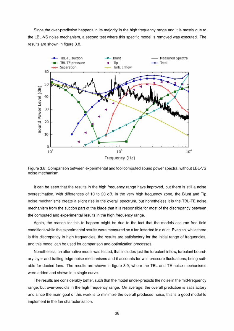
Since the over-prediction happens in its majority in the high frequency range and it is mostly due to
the LBL-VS noise mechanism, a second test where this specific model is removed was executed. The
results are shown in figure 3.8.
Figure 3.8: Comparison between experimental and tool computed sound power spectra, without LBL-VSnoise mechanism.
It can be seen that the results in the high frequency range have improved, but there is still a noise
overestimation, with differences of 10 to 20 dB. In the very high frequency zone, the Blunt and Tip
noise mechanisms create a slight rise in the overall spectrum, but nonetheless it is the TBL-TE noise
mechanism from the suction part of the blade that it is responsible for most of the discrepancy between
the computed and experimental results in the high frequency range.
Again, the reason for this to happen might be due to the fact that the models assume free field
conditions while the experimental results were measured on a fan inserted in a duct. Even so, while there
is this discrepancy in high frequencies, the results are satisfactory for the initial range of frequencies,
and this model can be used for comparison and optimization processes.
Nonetheless, an alternative model was tested, that includes just the turbulent inflow, turbulent bound-
ary layer and trailing edge noise mechanisms and it accounts for wall pressure fluctuations, being suit-
able for ducted fans. The results are shown in figure 3.9, where the TBL and TE noise mechanisms
were added and shown in a single curve.
The results are considerably better, such that the model under-predicts the noise in the mid-frequency
range, but over-predicts in the high frequency range. On average, the overall prediction is satisfactory
and since the main goal of this work is to minimize the overall produced noise, this is a good model to
implement in the fan characterization.
38

Figure 3.9: Comparison between experimental and tool computed sound power spectra.
However, since the behavior of the models studied in this chapter was compared to a fan in specific
ducted conditions, both models will be used in Chapter 5 in order to choose which one has a better
correlation with the baseline fan experimental data, by fine-tuning the custom tool.
39

40

Chapter 4
Blade Parametrization
In order to execute an aeroacoustic analysis of a fan, the geometry of the blades has to be properly
defined. While there are varied methods to accomplish this, in this work, where the objective is to
optimize the fan, there is an interest in describing the blades geometry with the least possible amount
of input parameters, such that the optimizer running time is kept to a minimum and the optimization is
done efficiently.
4.1 Airfoil Description
There are numerous methods available in the literature to parameterize an airfoil, such as PARSEC air-
foils, B-splines, NURBS, Bezier curves, Bezier-PARSEC parameterization, among others. An extensive
review of some of these methods is presented in [39] and [40].
As it was previously mentioned, the main criteria when choosing a parameterization method is to
minimize the number of design variables. In the work developed in [37], the parameterization of a wind
turbine blade profile was done using NURBS, leading to 20 as the chosen number of design variables
to describe the profile. This number is not restrictive, it could be higher or lower, but since it produced
successful results in the cited work, it will be used as a maximum threshold for the design variables used
to describe the airfoils in this work.
In [41], [42] and [43], is described a method in which the blade profile is built using a camber line and
a thickness curve, where the curvature and thickness distribution along the profile in the chord direction
is specified, respectively, with the profile the result of the junction of these curves. Both of these curves
are approximated by polynomials of a specified order, with the coefficients of the polynomials obtained
by relating them to the proposed design variables. Some of these variables are the maximum camber
and its location, the stagger angle, the maximum thickness and its location, among others. All of these
variables are expressed in figure 4.1. Although it is stated that this method only requires 14 design
parameters, due to the difficulty of measuring directly some of these parameters and the process of
reconstruction from a set of Cartesian coordinates to a parameterized configuration not being too clear,
this was not the chosen method.
41

Figure 4.1: Design variables defined in [41], [42] and [43].
In [44], a parameterization method which consists in combining Bezier curves and PARSEC airfoils is
presented. The driving principle behind this idea is to take advantage of the simplicity of implementation
of Bezier curves and its broad use in the CAD industry and combine it with the more aerodynamic-
oriented PARSEC parameterization scheme in order to avoid unrealistic or aerodynamic inefficient de-
signs in the optimizing process. The airfoil is described by four curves, two for the leading and trailing
edge camber lines and the other two for the leading and trailing edge thickness lines. These curves are
determined by four Bezier points each, making up a total sum of 16 control points, some of which are
fixed and the rest is a function of the defined aerodynamic parameters, namely the leading edge radius,
trailing and leading edge angles and position and curvature of thickness crest some examples of these
parameters. This method has a better convergence rate than most of the known methods, but it has a
minimum of 25 design variables per airfoil, not meeting the criteria established in this work to use this
method to parameterize the blade.
Following the method described before, the choice was made to test if Bezier curves were fit to
parameterize the blade profiles.
A Bezier curve is a parametric curve defined by
B(t) =
n∑I=0
bi,n(t)Pi, t ∈ [0, 1] , (4.1)
where
bi,n(t) =
(n
i
)ti(1− t)n−i and
(n
i
)ti(1− t)n−i =
n!
i!(n− i)!. (4.2)
In equation (4.1), Pi is a vector containing the control points which define a Bezier curve, the polyno-
mials represented by bi,n(t) are known as the Bernstein polynomials and t is the parametric variable
which ”runs along” the curve, such that t = 0 and t = 1 refers to the beginning and end of the curve,
respectively. The order of these curves is defined by the number of control points n + 1, such that the
42

Figure 4.2: Design variables of the Bezier-PARSEC parameterization method [44].
−0.2 0 0.2 0.4 0.6 0.8 1 1.2−0.8
−0.6
−0.4
−0.2
0Original S.C.Approx.Original P.S.
Figure 4.3: Failed test to fit 3rd order Bezier curves to one of the blade profiles.
order of the curve is always n. One of the properties of Bezier curves is that a given curve will always
contain the first and last control points, with the curvature and topology of the curve a consequence of
the location and number of the rest of the control points.
Given one of the blade profiles, obtained by sectioning it near the hub, it was attempted to fit the
coordinates of said profile with two 3rd degree Bezier curves, one for the suction part and the other for
the pressure part of the profile. This was done by minimizing the least-squares function between the
profile and the interpolated coordinates, in order to minimize the overall distance between the curves
and the original points. That fit was unsuccessful, as shown in figure 4.3, being that the leading and
trailing edges do not connect maybe due to the low order of the curves and the high curvature of the
pressure section trailing edge.
So, a second attempt was made by increasing the order of the Bezier curve which describes the
pressure part of the profile, due to having the curvature referred previously, from a 3rd to a 6th order
43
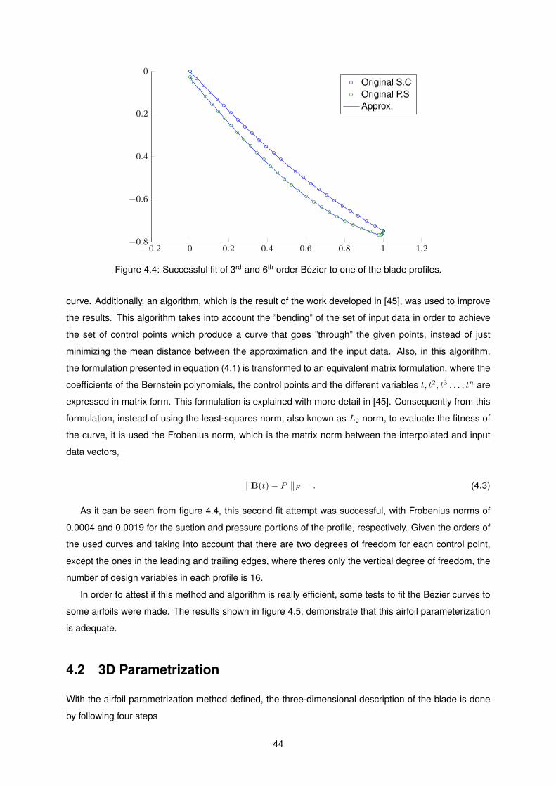
−0.2 0 0.2 0.4 0.6 0.8 1 1.2−0.8
−0.6
−0.4
−0.2
0Original S.COriginal P.SApprox.
Figure 4.4: Successful fit of 3rd and 6th order Bezier to one of the blade profiles.
curve. Additionally, an algorithm, which is the result of the work developed in [45], was used to improve
the results. This algorithm takes into account the ”bending” of the set of input data in order to achieve
the set of control points which produce a curve that goes ”through” the given points, instead of just
minimizing the mean distance between the approximation and the input data. Also, in this algorithm,
the formulation presented in equation (4.1) is transformed to an equivalent matrix formulation, where the
coefficients of the Bernstein polynomials, the control points and the different variables t, t2, t3 . . . , tn are
expressed in matrix form. This formulation is explained with more detail in [45]. Consequently from this
formulation, instead of using the least-squares norm, also known as L2 norm, to evaluate the fitness of
the curve, it is used the Frobenius norm, which is the matrix norm between the interpolated and input
data vectors,
‖ B(t)− P ‖F . (4.3)
As it can be seen from figure 4.4, this second fit attempt was successful, with Frobenius norms of
0.0004 and 0.0019 for the suction and pressure portions of the profile, respectively. Given the orders of
the used curves and taking into account that there are two degrees of freedom for each control point,
except the ones in the leading and trailing edges, where theres only the vertical degree of freedom, the
number of design variables in each profile is 16.
In order to attest if this method and algorithm is really efficient, some tests to fit the Bezier curves to
some airfoils were made. The results shown in figure 4.5, demonstrate that this airfoil parameterization
is adequate.
4.2 3D Parametrization
With the airfoil parametrization method defined, the three-dimensional description of the blade is done
by following four steps
44

−0.2 0 0.2 0.4 0.6 0.8 1 1.2
0
5 · 10−2
0.1Original S.COriginal P.SApprox.
(a) NACA 6409
−0.2 0 0.2 0.4 0.6 0.8 1 1.2
−5 · 10−2
0
5 · 10−2
0.1 Original S.COriginal P.SApprox.
(b) Eppler E1212
−0.2 0 0.2 0.4 0.6 0.8 1 1.2−0.2
−0.1
0
0.1Original S.COriginal P.SApprox.
(c) NREL 809
Figure 4.5: Fitting of Bezier curves to some airfoils.
45

Figure 4.6: Twist and chord distribution example.
1. Obtain the radial distribution of airfoil shapes of the blade, with all of the airfoils having unit chord;
2. Connect these airfoils to form the blade basis;
3. Apply the chord distribution by scaling each airfoil according to their local chord value;
4. Apply the twist distribution by rotating each airfoil with respect to their aerodynamic center (located
per default at 14 chord, but it is customizable by the user).
The chord and twist distributions are obtained by linear interpolation between the airfoils or, if an higher
order curve is needed to define the distribution, by creating control points to build a Bezier curve which
will express them in a continuous function. Examples of these distributions are shown in figure 4.6.
With this approach, there is the advantage of the airfoil locations, twist and chord distributions being
independent among themselves, allowing for their separate optimization in order to study the impact of
each variable in the final results.
46

Chapter 5
Baseline Fan Characterization
In this chapter, the geometry of the baseline fan which will be optimized and the process to input it in
the aeroacoustic code is presented. An aeroacoustic analysis of the fan is executed using two different
methods, and an experimental correlation between the results obtained by the code and the experimen-
tal measures is done.
5.1 Blade Definition
The geometry of the fan was provided by an air conditioning manufacturer to the author in the form of a
CAD file, which was edited in Solidworks. Figure 5.1 shows the different views of the 3D model of the
fan. The hub and fan radius were measured in the model and are resumed in table 5.1.
Unlike a typical turbine blade, this fan blade is not defined by one or a set of previously known airfoils,
such as the airfoil shape variable along the radius. Therefore, the number of airfoils to be extracted from
the model along the radius has to be chosen in order to describe effectively the fan blade shape inside
the aeroacoustic tool.
In a first approach, the intention was to gradually increase the number of extracted airfoils and com-
pare the geometry produced by the tool with the original geometry by overlapping them, but since the
formats of the information of both geometries are widely different, it was not possible to introduce them
simultaneously in the same context.
An alternative method was chosen, where an image of the top view of the blade was scanned in
such a way that a set of points for each edge of the blade was obtained, as shown in figure 5.2. A
coordinate system was temporarily set, with the x axis coincident with the axis shown in the figure and
the y axis being in the vertical direction. Then, the distance between points with the same x coordinate
Radius (m)Hub 0.0733Fan 0.225
Table 5.1: Fan and hub radius.
47

(a) Frontal view
(b) Lateral view
(c) 3D view
Figure 5.1: Views of the baseline fan model.
48

Figure 5.2: Set of points used to estimate the minimum number of extracted airfoils.
Bezier curve order Frobenius Norm2 0.01803 0.01114 3.5527E-155 3.4262E-146 2.5864E-14
Table 5.2: Results of Bezier curve fits to determine the number of extracted airfoil sections.
was computed in order to have a set of values which translate the distance between the two edges along
the radial coordinate.
Using the algorithm referred in Chapter 4, a Bezier curve was fitted to these sets of points with the
intent of finding the minimum order of the curve which has the best possible fit with the data. This way
if, for example, a 2nd order Bezier curve has a satisfactory fit, it is only necessary 3 control points, or 3
airfoils, in this case, to describe the distance between the edges of the blade.
In table 5.2, the results of a series of tests to fit a Bezier curve to the data are shown. It can be seen
that between the 3rd and 4th order, there is a considerable decrease in the Frobenius norm, while in the
5th and 6th order the norm increases, although having values of the same magnitude as the 4th order
norm. Since the order with the lowest norm is the 4th, this Bezier curve order is the one which produces
the best fit to the blade curvature, with 5 control points. Therefore, 5 airfoil shapes were extracted along
the radial position and introduced into the aeroacoustic tool in order to replicate the original geometry.
49

(a) Airfoil 1 (r/R = 0.33)
(b) Airfoil 2 (r/R = 0.49)
(c) Airfoil 3 (r/R = 0.72)
(d) Airfoil 4 (r/R = 0.82)
(e) Airfoil 5 (r/R = 0.93)
Figure 5.3: Airfoil sections extracted from the blade.
Figure 5.4: Location of extracted airfoils in the blade model.
Before the extraction of the airfoil sections, the leading edge of the blade had to be changed, by
rounding it with a radius of 0.1 mm. The reason behind this is explained in Section 5.2. The sections
were obtained by sectioning the model in Solidworks and by scanning the image in the same way as
before and obtaining a set of points which described each section, being these points saved in a .dat
file to input in the code. All of the airfoils are normalized to unit chord. The extracted airfoils and their
location in the blade are shown in figures 5.3 and 5.4.
Since the tool has the option of inputing the chord and twist distributions as a Bezier curve, the chord
and twist of each airfoil were measured and using once again the Bezier fitting algorithm used throughout
this work, two Bezier curves were obtained which translate the blade chord and twist distributions.
The process of building the geometry of a blade includes the connection of the airfoil shapes using
an invisible reference line that passes through a specified point on each of the airfoil shapes. Per default,
50

# of Airfoil % chord1 71.52 64.453 42.84 43.335 40.39
Table 5.3: Locations of the points in each airfoil upon which the reference line used to build the bladepasses through.
Parameter ValueNumber of blades 3
Rotational speed (rpm) 850Axial flow velocity (m/s) 10.55
Trailing edge angle (deg) 2Turbulence intensity (%) 2
Turbulence length scale (m) 0.002
Table 5.4: Parameters used in baseline fan aeroacoustic analysis.
this point is located as 25% of the chord from the leading edge, but it can be defined as input from the
user. In this case, these points were calculated and extracted from the model for each section. The
locations of these points, expressed in percentage of chord, are presented in table 5.3.
With all of the geometric parameters defined and introduced in the code, the final blade geometry
was produced by the program. A reproduction of the model with 30 control sections equally spaced is
shown in figure 5.5. Two views from two different perspectives are presented.
5.2 Aeroacoustic Analysis
With the blade geometry defined, an aeroacoustic analysis was executed to characterize the nominal
noise levels of the fan. The analysis parameters are shown in table 5.4. The turbulence parameters are
merely indicative, being adjusted to correlate with the experimental data in Section 5.3.
Before the analysis could be executed, it was necessary to supply the aerodynamic polars for each
extracted airfoil to the code in order for the BEM code to have the required data to compute the in-
duced velocities along the blade radius. Since it is linked to this tool, XFOIL was used to obtain these
aerodynamic polars.
In Section 5.1, it was referred that the blade leading edge had to be rounded. This is due to the fact
that the original supplied geometry had a sharp-cornered leading edge, which implies airfoil sections
with sharp-cornered leading edges. Since the panel code used in XFOIL to predict the aerodynamic
coefficients of airfoils is highly sensible to the smoothness of the leading edge and the distribution of
points (or panels) in this area, it was unable to analyze the original airfoils. Hence the change in the
blade geometry, which, nonetheless, will not introduce an error factor when comparing the results with
the experimental data since the curvature radius is very small when compared to the length scale of the
airfoils, as it can be seen in figure 5.6, where a distance of 1 mm is presented for scale comparison.
51

Figure 5.5: Blade geometry produced by the aeroacoustic tool.
52

(a) Airfoil full view
(b) Airfoil 1/4 chord view
(c) Magnified view of the airfoil leading edge
Figure 5.6: Comparison between original and modified blade geometry.
With this new geometry, the required polars were computed and introduced in the code and the analysis
was executed.
The two models referred in Chapter 3 were used in two different analysis in order to choose which
one produces the results closest to the experimental data. The results obtained and the correlation is
done in the following section.
5.3 Experimental Correlation
In this section, the experimental results to which the noise predictions are correlated were obtained
from a floor standing AC unit with two fans, as the one shown in figure 5.7. The supplied experimental
spectra were measured by three microphones with the layout presented in figure 5.8. Each microphone
was labeled with a channel number, ranging from Channel 9 to Channel 12 and in this section, the
measurements which will be taken as the baseline are the ones obtained by Channel 10.
It is assumed that the two fans are noise sources with a mutually incoherent sound radiation and
have the same intensity, therefore the total noise produced by both fans can be obtained by adding
3 dB(A) to the results computed by the tool. Following this reasoning, all of the results presented in
53

Figure 5.7: Example of a floor standing AC unit (Copyrighted by LG).
AC Unit1 m 1 m
1 m
Ch. 9
Ch. 10
Ch. 12
(a) Top view
Ch. 9 Ch. 12
Ch. 10
(b) Front view
Figure 5.8: Schematic of the experimental setup for the supplied data.
54
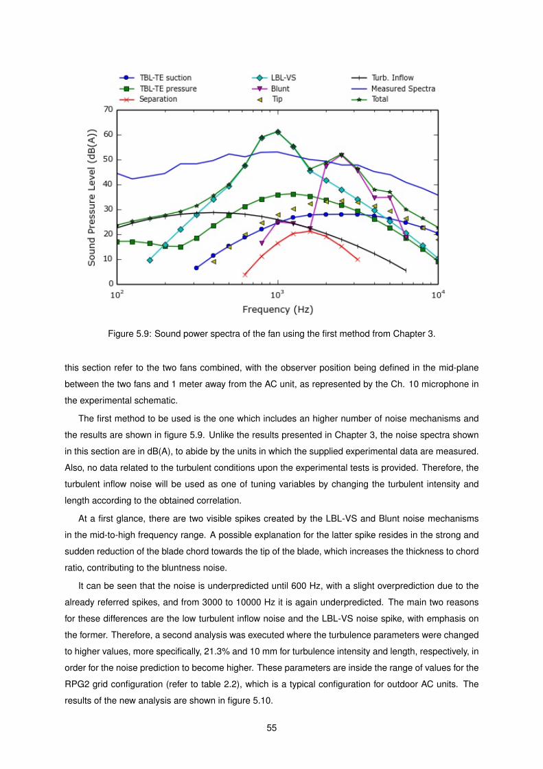
Figure 5.9: Sound power spectra of the fan using the first method from Chapter 3.
this section refer to the two fans combined, with the observer position being defined in the mid-plane
between the two fans and 1 meter away from the AC unit, as represented by the Ch. 10 microphone in
the experimental schematic.
The first method to be used is the one which includes an higher number of noise mechanisms and
the results are shown in figure 5.9. Unlike the results presented in Chapter 3, the noise spectra shown
in this section are in dB(A), to abide by the units in which the supplied experimental data are measured.
Also, no data related to the turbulent conditions upon the experimental tests is provided. Therefore, the
turbulent inflow noise will be used as one of tuning variables by changing the turbulent intensity and
length according to the obtained correlation.
At a first glance, there are two visible spikes created by the LBL-VS and Blunt noise mechanisms
in the mid-to-high frequency range. A possible explanation for the latter spike resides in the strong and
sudden reduction of the blade chord towards the tip of the blade, which increases the thickness to chord
ratio, contributing to the bluntness noise.
It can be seen that the noise is underpredicted until 600 Hz, with a slight overprediction due to the
already referred spikes, and from 3000 to 10000 Hz it is again underpredicted. The main two reasons
for these differences are the low turbulent inflow noise and the LBL-VS noise spike, with emphasis on
the former. Therefore, a second analysis was executed where the turbulence parameters were changed
to higher values, more specifically, 21.3% and 10 mm for turbulence intensity and length, respectively, in
order for the noise prediction to become higher. These parameters are inside the range of values for the
RPG2 grid configuration (refer to table 2.2), which is a typical configuration for outdoor AC units. The
results of the new analysis are shown in figure 5.10.
55

Figure 5.10: Sound power spectra of the fan using the first method with turbulence corrections.
The overall correlation with the experimental results is acceptable, although there are discrepancies
in the mid and high frequency zone. In the latter case, there is nothing that can be done to improve the
correlation, but in the mid-frequency case, it can be seen that the LBL-VS mechanism is responsible for
the overprediction in this area. So, a third analysis where this mechanism is not considered is executed,
being the results shown in figure 5.11.
Without the LBL-VS spike, the discrepancy between the noise prediction and the experimental results
in the mid-frequency area is still visible, although in this case, the noise is underpredicted. Since the
value of the discrepancy similar in both cases, the criteria to choose the method has to be the predicted
OASPL and it has to be compared to the experimental. This comparison will be presented after the
second method is tested.
In figure 5.12, the results of the second, simpler method are shown. The turbulence parameters from
the last analysis were maintained.
Although the discrepancy in the low frequency zone is acceptable, the correlation in the remaining
spectrum is not satisfactory, with differences of the order of 20 dB(A) between the predicted and the
experimental results. Since the turbulent inflow noise is the only tuning parameter in this method and
the turbulent parameters are already in its maximum, the correlation cannot be improved.
In table 5.5, the values of OASPL obtained by the two variations of the first method and the second
method are presented, along with the error when compared to the OASPL supplied by the air condition-
ing manufacturer of 61.4 dB(A).
Since the first method, without the LBL-VS noise mechanism, has the lowest error and it takes into
account an higher number of noise mechanisms, it will be the chosen method for the subsequent studies
56

Figure 5.11: Sound power spectra of the fan using the first method without LBL-VS noise mechanismand with turbulence corrections.
Figure 5.12: Sound power spectra of the fan using the second method from chapter 3.
57

Method OASPL (dB(A)) Error (%)First (with LBL-VS) 65.5 6.67
First (without LBL-VS) 60.1 2.12Second 58.7 4.34
Table 5.5: OASPL calculated by the considered methods and comparison to nominal OASPL.
of the fan.
58

Chapter 6
Geometrical Parametric Study
With the noise model chosen and the baseline values defined, a study on the impact of the variation
of the fan diameter and number of blades in the produced noise was conducted. Three cases were
considered: one where the baseline number of blades is maintained and the diameter is changed, other
with the baseline diameter unchanged and variation of number of blades and the last with a simultaneous
change in both geometrical variables.
6.1 Fan Diameter
In order for the blades to be geometrically similar while changing the fan diameter, the hub and blade
tip radius were changed by the same ratio, maintaining the distance between the two blade extremities.
Also, the baseline twist and chord distributions were translated by the same factor applied in the hub and
blade tip. Therefore, the relative distance between the control sections and points was kept unchanged
along with the respective chord and twist values, being only their radial coordinate the parameter to be
altered.
While changing the fan diameter, the volumetric air flow has to be constant. Therefore, an increase
or decrease in the diameter translates in a decrease or increase in the axial velocity, according to
V =1.5
π(R2tip −R2
hub), (6.1)
where V is the axial velocity,Rtip and Rhub are the tip and hub radius, respectively and the value of 1.5
is due to the design imposition of maintaining a volumetric flow of 1.5 m3/s.
These changes also imply that the power consumed by the fan is unaltered, being the decrease of
the fan rotational speed a consequence of the increase of the diameter. The relation between these two
variables can be obtained using dimensional analysis, resulting in the relation of proportionality between
the fan power and the following expression,
P ∼ ρND5Ω3 , (6.2)
59

with ρ as the air density, N as the number of blades, D as the diameter and Ω as the rotational speed.
Therefore, for the same consumed power, the relation between the rotation speed of a fan 1 and a
fan 2 is given by
Ω2 = Ω1
(N1
N2
D51
D52
)1/3
. (6.3)
Since in the present case, the number of blades stays the same, equation (6.3) reduces to
Ω2 = Ω1
(D1
D2
)5/3
. (6.4)
Using the presented expressions, the rotational speeds and axial velocities used in the analysis for
each diameter value were obtained and are presented in table 6.1. The diameter was changed in the
range from 400 mm to 600 mm. The values for the baseline fan are shown in bold.
Diameter (mm) Axial velocity (m/s) Rotational speed (RPM)400 12.68 1034450 10.55 850470 9.89 791500 9.04 713550 7.9 608600 7.02 526
Table 6.1: Axial velocity and rotational speed values for different fan diameters.
After inputing these parameters and making the necessary geometrical changes in the aeroacoustic
tool, the noise predictions were obtained and are shown in table 6.2. The noise spectra for each diameter
are presented in figure 6.1. The values for the baseline fan are shown in bold.
Diameter (mm) Noise (dB(A))400 64.96450 60.09470 58.49500 56.91550 55.34600 54.16
Table 6.2: Noise predictions for various diameters.
The increase in diameter translates into a decrease in the produced noise and a reduction of 5.9
dB(A), which equals 9.6 %, is obtained for a diameter of 600 mm when compared to the baseline case
of 450 mm.
When analyzing the spectra comparison, it can be seen that the peak observed originally at around
2500 Hz for the 450 mm diameter, descends to lower frequencies with the increase of diameter. This can
be explained by the fact that the wavelength of the fundamental vibration mode of a body is proportional
to its dimensions, therefore for a bigger fan, the wavelength is higher and the frequency is lower.
60

Figure 6.1: Sound pressure level spectra for each fan diameter.
6.2 Blade Number
When the number of blades is changed, the equivalent blade area has to remain the same in order for
the comparison to be valid or else it would be added additional area that was not in the fan initially. This
implies that for an increase in the number of blades while maintaining the diameter, the mean blade
chord has to decrease.
Therefore, the following relation between the blade chord c and the number of blades N of two fans
1 and 2 was used:
c2 = c1N1
N2. (6.5)
From equation (6.5), the chord values of the 5 control sections for each fan with different number
of blades were obtained. A Bezier curve was fitted in these values, in order to obtain the new chord
distribution of the new blades, following the same procedure used in the baseline fan.
Similarly to the fan diameter, a change in the number of blades also affects the rotational speed if the
consumed power is to be the same, as shown by equation (6.3). For a constant diameter, the equation
used is
Ω2 = Ω1
(N1
N2
)1/3
. (6.6)
The range of study for the number of blades was from 3 to 6 blades and the baseline diameter of 450
mm was used. The rotational speeds used in each analysis are presented in table 6.3, the predicted
noise is shown in table 6.4 and the noise spectra for each number of blades are present in figure 6.2.
The baseline values are shown in bold.
61

Number of blades Rotational speed (RPM)3 8504 7725 7176 675
Table 6.3: Rotational speeds for different number of blades.
Number of blades Noise (dB(A))3 60.14 60.15 58.96 58.4
Table 6.4: Noise predictions for different number of blades.
Similarly to the effect of the increase of diameter, the increase of blade number reduces the produced
noise, although the magnitude of the reduction is lower than the observed when increasing the diameter.
With 6 blades, a noise reduction of 1.7 dB(A) was obtained, which translates into a variation of 2.8%.
Figure 6.2: Sound pressure level spectra for each blade number.
When comparing the noise spectra, it can be noted that the peak observed around 3000 Hz stays
relatively unchanged, with the exception of the 3 blades case. This can be explained following the same
reasoning presented in Section 6.1, since only the number of blades is altered, hence the characteristic
dimensions of the fan are unchanged and the frequency where the peak manifests itself is the same.
Therefore, the main reason for the noise reduction is found in the low-to-mid frequency zone, where
the dominant noise mechanism, the turbulent inflow noise, is decreased along with the increase in the
62

number of blades.
6.3 Fan Diameter and Blade Number
Using all of the relations presented in the previous sections, a parametric study where the two variables
present in this chapter are changed simultaneously was conducted. The rotational speeds used for each
pair of variables are shown in table 6.5 and the respective noise predictions are presented in table 6.6.
Also, the baseline values are shown in bold.
Diameter (mm)Blade number
3 4 5 6
400 1034 940 872 821
450 850 772 717 675
470 791 718 667 628
500 713 648 602 566
550 608 553 513 483
600 526 478 444 418
Table 6.5: Rotational speeds (RPM) for different number of blades and diameters.
Diameter (mm)Blade number
3 4 5 6
400 65.0 64.0 62.1 60.0
450 60.1 60.1 58.9 58.4
470 58.5 57.1 59.1 58.6
500 56.9 58.1 57.6 57.2
550 55.3 54.8 53.8 52.3
600 54.2 52.5 51.1 50.2
Table 6.6: Noise predictions (dB(A)) for different number of blades and diameters.
The conclusions inferred from the previous sections agree with the presented values, although there
are some exceptions. For the 470 mm diameter, there is an increase of noise from 4 to 5 blades and
the same is verified for the 500 mm diameter and from 3 to 4 blades. However, it can be seen that in a
general sense, the increase in fan diameter and number of blades results in a reduction of the produced
noise, being possible to reduce it up to 16.5%.
63

Along with the noise, it was also possible to compute the fan efficiency for each case, being the
results presented in table 6.7.
Diameter (mm)Blade number
3 4 5 6
400 14.4 9.8 4.7 3.6
450 22.2 13.2 27.2 3
470 22.7 10 5.6 2.1
500 25.5 30.5 11.3 1.8
550 24.7 33.1 3 1.7
600 29.5 18.2 3.1 2
Table 6.7: Fan efficiency (%) for different number of blades and diameters.
In a general sense, an increase in diameter results in an increase on efficiency, while an increase in
blade number impacts it negatively, although there are some inconsistencies, as in the noise predictions.
There is a raise in efficiency when the blades increase from 4 to 5, in the 450 mm diameter case, and
from 3 to 4, in the 500 and 550 mm diameter cases. These deviations can be explained by reduction in
rotational speed and chord when the blade number increases and by the reduction in axial flow velocity
when the diameter increases, because lower chords and lower speeds lead to stall being achieved more
quickly, which introduces imprecisions in the calculations. Nonetheless, the final results refer to the
averaged sum of all blade elements and therefore, they are trustworthy.
The low efficiency values are explained by the following logic; both diameter and blade number
changes are applied with the assumption that the power consumed by the fan stays the same, which
coupled to the reduction of rotational speed, implies that the torque increases. Also, with the blade
number increase, the blade chord decreases. From equation (2.59), it can be seen that with the reduction
in rotational speed and chord, while maintaining the axial flow velocity, the inflow angle has to decrease
in order for the torque to increase. Referring to equation (2.55), the only way to decrease the inflow
angle, with decreasing rotational speed, is to decrease both the axial and radial induction factors. It can
be seen that this decreases the produced thrust, by inspecting equation (2.58), which in turn decreases
efficiency, with constant power and axial flow velocity (see equation (2.70)).
Combining tables 6.6 and 6.7, it is visible that the best trade-off solution lies between the 500 and
550 mm diameter and 3 and 4 blades.
64

Chapter 7
Aeroacoustic Fan Optimization
In this chapter, the final optimization of the fan will be performed. An overview of the existing optimization
techniques and the choice of the method used in this work will be presented. The aeroacoustic opti-
mization problem is defined in terms of constraints and design variables and finally, several optimization
cases are set up and the respective results will be presented.
7.1 Numerical Optimization Techniques
Contrary to diameter and number of blades, the blade chord, twist and curvature are continuous vari-
ables and change with the radial coordinate, which turns a parametric study similar to the ones in chapter
6 a difficult task to perform. Therefore, a numerical optimization algorithm had to be chosen and applied
to these variables in order to obtain a final solution.
In the field of numerical optimization, the available methods can be divided in two categories: de-
terministic and heuristic. Deterministic methods rely upon an analytical definition of the problem to
generate a set of points which converge towards a local optimal solution, while heuristic methods mimic
some of the phenomena found in nature to find the global optimal solution. Some examples of determin-
istic methods are Linear Programming, Nonlinear Programming or Sequential Quadratic Programming
(SQP). The heuristic category includes methods such as Genetic Algorithms, Ant Colonies, Differential
Evolution, Particle Swarm, etc. A thorough review of optimization methods can be found in [46].
Generally, heuristic methods are more powerful and flexible than deterministic methods and have the
advantage of being iterative, not requiring an analytical definition of the objective function. However, they
have an higher computational cost, the quality of the solution cannot be guaranteed and the probability of
finding a global optimum solution decreases with the increase in design variables. Nonetheless, when
a relation between the objective and the design variables cannot be analytically defined, an heuristic
method is the best choice.
Given the advantages of genetic algorithms and their presence in many engineering single and multi-
objective optimization problems [47], the NSGA-II [48] (Non-Dominated Sorting Genetic Algorithm) was
the optimization algorithm chosen for the optimizations present in this chapter. It solves non-convex
65

and non-smooth single and multi-objective optimization problems. This algorithm was already used in
multi-objective aeroacoustic optimization of wind turbine blades [49].
The NSGA-II is already included in pyOpt, a Python-based optimization framework used for formulat-
ing and solving nonlinear constrained (and unconstrained) optimization problems [50]. The advantage of
using pyOpt is the fact that the process of establishing an optimization problem is as simple as defining
a function which takes as input a vector with the design variables and outputs the objective functions(s)
and constraint(s) to the optimizer. After the function is defined, the optimization problem can be initialized
with the naming of the design variables and defining their constraints.
Convergence of the solution One of the input parameters in an optimization using genetic algorithms
is the size of the population that is created in each generation. Another input is the number of gener-
ations, which functions as the stopping criteria for the optimizer. These two parameters influence the
convergence of the solution, since if they are too low, the solution might not converge and there is still
more leeway in the design space to achieve a better solution. However, if these numbers are too high,
there can be a waste of computational resources, since the solution might already have converged, but
the optimizer is still running until it reaches the maximum number of generations. Therefore, a conver-
gence study was conducted for each optimization case in Section 7.3.
In [37], it was studied the impact of the population size in the convergence and on the running time.
As expected, with the increase of the population size, the number of generations required to achieve
convergence is lower, but the necessary number of function calls is higher. Since the CPU time is
directly proportional to the number of function calls, it was concluded that a population size between n
and 2n (with n as the number of design variables) can guarantee a converged solution with an efficient
use of computational resources for a shorter runtime. Given that the basis of the work which led to this
conclusion is similar to the basis of this work, this rule of thumb will also be applied in the subsequent
optimizations.
7.2 Problem Definition
Every optimization problem consists on minimizing (or maximizing) an objective function, which is de-
pendent of a set of design variables subject to a series of constraints. A typical mathematical formulation
for these problems is
minimizex
f(x)
subject to g(x) ≤ ai, i = 1, . . . ,m
h(x) = bj , j = 1, . . . , n
xLk < xk < xUk , k = 1, . . . , p
where f(x) is the objective function, x is the design vector, g(x) are the inequality constraints and h(x)
are the equality constraints. Each variable xk in the design vector is constrained by a lower value xLk
and by an upper value xUk . These are referred to as side constraints.
66

In the several optimization cases presented in the next section, there will be performed single and
multi-objective optimizations of two objective functions: the overall produced noise (OASPL) and the
fan efficiency (see Section 2.6.2). The design variables will be the location of the control points which
compose the Bezier curves of the chord and twist distributions and the locations of the 5 control sections
in terms of chord percentage in order to change the blade curvature. There will be no inequality and
equality constraints and the side constraints for each design variable will be stated for each optimization
case.
7.3 Optimization Cases
The optimization simulations were conducted on two fans: the baseline fan and an improved fan from
the results obtained in Chapter 6, more specifically, the 550 mm diameter fan with 6 blades.
For each fan, the impact of the chord and twist design variables in minimizing the produced noise,
maximizing the efficiency and in the trade-off between these two objective functions was studied sep-
arately. In the case of the curvature, only the impact in the noise was addressed, since one of the
disadvantages of the BEM implementation is that each blade element is considered independent of the
neighboring elements and thus the fan efficiency is unaffected by the change in the blade curvature.
Afterwards, it was assessed the effect of optimizing simultaneously the blade chord and twist for the
two objectives, both mutually and exclusively. Finally, the chord, twist and curvature were optimized for
minimizing the noise. The efficiency was not considered for the reasons already stated above.
The parameters for each analysis were the same as the ones used in Chapter 5, including the
turbulence parameters and the observer position.
7.3.1 Baseline Fan
The noise and efficiency values of the baseline fan are presented in table 7.1 as reference for the
comparison with the results.
Noise(dB(A)) Efficiency (%)60.1 22.2
Table 7.1: Noise and efficiency values for baseline fan.
Chord The first optimization to be considered is the optimization of the blade chord. The chord distri-
bution is defined by a 6th order Bezier curve and since the locations of the curve control points are the
design variables, except for the radial coordinates of endpoints, the total number of design variables for
the chord optimization is 10.
In all analysis, the chord values and radial positions were constrained between 90% and 110% of
67

Figure 7.1: Variation of population average and best OASPL with the number of generations with chordas the design variable.
their initial values:0.9 cinitiali < ycpi < 1.1 cinitiali
0.9ri
Rmax< xcpi < 1.1
riRmax
(7.1)
The first objective was the OASPL and the optimization resulted in a decrease of the noise down to
58.42 dB(A). The convergence study is presented in figure 7.1 and it can be considered that the solution
converges. The optimized chord distribution is shown in figure 7.2.
The new chord distribution translates into a blade with a lower chord, which was expected as the
noise production for each element is a function of the boundary thickness parameters, which are propor-
tional to the element chord. It is interesting to note that while up until the maximum chord at r/R = 0.77,
the chord increase rate is the same as in the initial distribution, from the maximum until the end, the
chord decreases in a more linear rate than the initial, with the reduction towards the end less sudden.
This indicates that a smooth transition in the chord at the tip area is a factor to take into account when
minimizing the noise.
Although this optimization did only account for the noise, the efficiency of the optimized fan was
computed in order to assess the trade-off between the impact on noise and the aerodynamic impact.
This optimization resulted in an efficiency decrease of 1.6%, with the optimized fan having an efficiency
of 20.6%.
A second optimization was conducted, with the efficiency as the objective function. The optimization
converged, as seen in figure 7.3, and resulted in an increase up to 26.1%. The optimized chord distri-
bution is presented in figure 7.4. The optimized chord distribution is similar to the initial, although the
maximum chord is lower, indicating that the original geometry is already near the optimal aerodynamic
design. The overall reduction of the chord is explained by the fact that the chord is proportional to the
consumed power by the fan, so that a reduction of chord implies an increase in efficiency. This increase
68

0.3 0.35 0.4 0.45 0.5 0.55 0.6 0.65 0.7 0.75 0.8 0.85 0.9 0.95 10
5 · 10−2
0.1
0.15
0.2
0.25
0.3
0.35
r/R
Cho
rd(m
)
InitialBest OASPL
Figure 7.2: Comparison between the initial and the best OASPL chord distribution.
in efficiency also incurred into a decrease of 0.6 dB(A) to 59.5 dB(A).
Figure 7.3: Variation of population average and best efficiency with the number of generations with chordas the design variable.
The final chord optimization had both the OASPL and efficiency as objective functions. The optimizer
provided a set of solutions from a dispersed set and the resulting Pareto front is presented in figure 7.5.
It is visible from the figure that there is room for improvement in minimizing the noise, even in the solution
for the maximum efficiency. The trade-off solution results in an OASPL of 58.25 dB(A) and an efficiency
of 26.4% and the respective chord distribution is shown in figure 7.6. The trade-off chord distribution is a
combination of the previous distributions, with a lower maximum (and overall) chord value and a similar
growth rate than the initial distribution.
69

0.3 0.35 0.4 0.45 0.5 0.55 0.6 0.65 0.7 0.75 0.8 0.85 0.9 0.95 15 · 10−2
0.1
0.15
0.2
0.25
0.3
0.35
0.4
r/R
Cho
rd(m
)
InitialBest Efficiency
Figure 7.4: Comparison between the initial and the best efficiency chord distribution.
Figure 7.5: Pareto front in chord multi-objective optimization case.
Twist The second main design variable is the blade twist. The twist distribution is defined by a 5th
order Bezier curve and the design variable procedure is the same as the one in the chord optimization,
which results in a total number of 8 design variables.
In all twist optimizations, the twist values were constrained between 85% and 115% of their initial
values, being the radial positions constraints the same as the ones in the chord optimization:
0.85 θinitiali < ycpi < 1.15 θinitiali
0.9ri
Rmax< xcpi < 1.1
riRmax
(7.2)
Following the same procedure as in the chord section, the first objective function was the OASPL,
being the convergence study shown in figure 7.7, resulting in a noise reduction down to 59.25 dB(A)
70

0.3 0.35 0.4 0.45 0.5 0.55 0.6 0.65 0.7 0.75 0.8 0.85 0.9 0.95 15 · 10−2
0.1
0.15
0.2
0.25
0.3
0.35
0.4
r/R
Cho
rd(m
)
InitialBest OASPL+Eff
Figure 7.6: Comparison between the initial and the trade-off solution chord distribution.
and, consequently, in an increase of efficiency to 22.8%. The optimal twist distribution is presented in
figure 7.8. It is visible that both distributions have a similar shape, with the optimized twist distribution
having lower twist values than the initial distribution. The reduction in the twist also reduces the effective
angle of attack along the blade radius, which explains the impact of minimizing the overall noise.
Figure 7.7: Variation of population average and best OASPL with the number of generations with twistas the design variable.
In the optimization for the efficiency objective function, the obtained results showed an increase of
2.3% to 24.5%, with the convergence study being presented in figure 7.9. The optimized twist distribution
is shown in figure 7.10. There is an abrupt change in the twist around r/R = 0.7, from where it increases
up to 34 degrees at the tip of the blade. The fact that this change happens around the tip area increases
the torque, since it is proportional to the element radius, but the impact it has in thrust is higher than
71
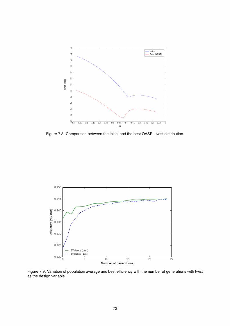
0.3 0.35 0.4 0.45 0.5 0.55 0.6 0.65 0.7 0.75 0.8 0.85 0.9 0.95 126
27
28
29
30
31
32
33
34
35
36
37
38
r/R
Twis
t(de
g)
InitialBest OASPL
Figure 7.8: Comparison between the initial and the best OASPL twist distribution.
Figure 7.9: Variation of population average and best efficiency with the number of generations with twistas the design variable.
72

0.3 0.35 0.4 0.45 0.5 0.55 0.6 0.65 0.7 0.75 0.8 0.85 0.9 0.95 126
27
28
29
30
31
32
33
34
35
36
37
38
r/R
Twis
t(de
g)
InitialBest Efficiency
Figure 7.10: Comparison between the initial and the best efficiency twist distribution.
the increase found in the torque due to the increase in the effective angle of attack. Therefore, the ratio
between thrust and torque is higher as well as the efficiency. However, since the highest levels of noise
production are found in the tip area, this twist increase impacts negatively the noise, which is balanced
by the lower twist around the hub area. In this case, the effect of the lower twist prevails since the overall
noise was reduced to 59.76 dB(A).
In the twist optimization of both objective functions, OASPL and Efficiency, the optimizer produced a
Pareto front which is shown in figure 7.11. As in the chord optimization case, it can be seen that even
for the case of maximum efficiency, there is potential to improve the fan noise levels, although it only
translates in a reduction of 0.3 dB(A). A greater reduction of almost 1 dB(A) is possible, with a penalty
in the efficiency, although it is still observed an increase compared to the initial case.
The twist distribution for the trade-off solution is presented in figure 7.12. Since the trade-off solution
is similar to the maximum efficiency solution, as seen in figure 7.11, it was expected that the twist
distribution was similar as well, being observed a sudden increase in the twist at the tip area.
Curvature Curvature is the third and last design variable to use in the optimization process. For the
reasons mentioned in the beginning of this section, the only objective function to be considered is the
OASPL. The curvature is defined by the locations of the control sections, which are constrained between
-10% and +10% of their initial positions expressed in chord percentage. The obtained results by the
optimizer showed a minimal decrease to 60.03 dB(A) and the respective control sections locations are
presented in table 7.2. In figure 7.13, the control sections are graphically represented, including the
temporary axis upon which the section locations are measured. From the three main design variables,
curvature is the one with a lesser impact in noise reduction, reducing it only by 0.1%. Adding that to the
fact the difficulty of changing the manufacturing process when changing the blade curvature surpasses
the minimal benefit in noise reduction, turning curvature into the less important of the three design
variables.
73

Figure 7.11: Pareto front in twist multi-objective optimization case.
0.3 0.35 0.4 0.45 0.5 0.55 0.6 0.65 0.7 0.75 0.8 0.85 0.9 0.95 126
27
28
29
30
31
32
33
34
35
36
37
38
r/R
Twis
t(de
g)
InitialBest OASPL + Efficiency
Figure 7.12: Comparison between the initial and the trade-off twist distribution.
# of Airfoil Baseline % chord Optimized % chord1 71.5 79.542 64.5 72.33 42.8 43.064 43.33 375 40.39 34
Table 7.2: Curvature optimization results.
74

Figure 7.13: Optimized locations of the control airfoil sections.
Chord and Twist With the chord and twist being considered simultaneously as design variables, the
solutions obtained by the optimizer for each objective function, separately, resulted in a decrease in
OASPL of 4.1% to 57.61 dB(A) and in an increase in efficiency of 5.3% to 27.5%. The respective chord
and twist distributions for each case are presented in figures 7.14 and 7.15.
25
27
30
33
35
Twis
t(de
g)
0.3 0.35 0.4 0.45 0.5 0.55 0.6 0.65 0.7 0.75 0.8 0.85 0.9 0.95 10
0.1
0.2
0.3
0.4
r/R
Cho
rd(m
)
Best OASPL TwistBest OASPL Chord
Figure 7.14: Chord and twist distribution for best OASPL.
The best OASPL distributions are similar to the best OASPL distributions for each separate design
variable, with a slight increase in twist between r/R = 0.7 and 0.75, which proves that their combination
takes advantage of their separate impact in minimizing noise.
In the best efficiency distributions, it can be seen that the tendency to increase twist towards the
tip area is again present, like in the twist-only case, although there is a slight reduction in the proximity
of the tip. The difference in the chord distribution in this case lies in the decrease rate between the
maximum chord and the tip, being that in all other chord optimization results decreased slowly from the
maximum and changed abruptly towards, while in this case the tip transition is smooth. The decrease in
75

29
30
31
32
Twis
t(de
g)
0.3 0.35 0.4 0.45 0.5 0.55 0.6 0.65 0.7 0.75 0.8 0.85 0.9 0.95 10.1
0.2
0.3
0.4
r/R
Cho
rd(m
)
Best Efficiency TwistBest Efficiency Chord
Figure 7.15: Chord and twist distribution for best efficiency.
twist coupled with this transition results in less torque when compared to the baseline case and although
the thrust is also diminished, the torque reduction is of higher proportions than the thrust and therefore
the efficiency is higher.
Chord, Twist and Curvature In the optimization with the combination of all design variables, it was
expected that the combined effect would produce the best results. However, it was observed that by
coupling the curvature with the twist and chord, the noise improvement brought by the latter combina-
tion was diminished, being the final result a reduction to 57.85 dB(A). The resulting chord and twist
distribution will not be presented, due to fact that it is similar to the one shown in figure 7.14, proving the
negative impact the curvature has when combined with chord and twist changes.
Summary of the Results
A summary of all the presented optimization results is shown in table 7.3, where it can be seen that the
solution involving the change of the chord and twist simultaneously produces the best overall results. It
presents the minimum noise, with 57.61 dB(A), which equals a 4.1% reduction, the maximum efficiency,
for an increase of 5.3% to 27.5% and the best trade-off, if the criteria is the minimum ratio between the
noise and efficiency.
Design Variable OASPL (dB(A)) Efficiency (%) OASPL + EfficiencyChord 58.42 26.1 58.25/26.4Twist 59.25 24.5 59.79/24.5
Chord+Twist 57.61 27.5 59.33/27.9Curvature 60.03 - -
Chord+Twist+Curvature 57.85 - -
Table 7.3: Summary of the optimization results for the baseline fan.
76

7.3.2 Improved Fan
After optimizing the baseline fan, the fan with the best noise results from Chapter 6, which is the 500 mm
diameter and 6 blade fan, was also subjected to the optimization process. Since all of the process was
followed exactly like in the baseline fan optimization, only a summary of the obtained results is presented
in table 7.4. For reference, the noise and efficiency baseline values for this fan are 52.3 dB(A) and 1.7%,
respectively. The low efficiency value is explained in Chapter 6.
Design Variable OASPL (dB(A)) Efficiency (%) OASPL + EfficiencyChord 50.08 2.2 50.56/1.7Twist 51.78 1.9 51.75/1.7
Chord+Twist 49.64 4.1 51.15/2.6Curvature 52.19 - -
Chord+Twist+Curvature 49.60 - -
Table 7.4: Summary of the optimization results for the 500 mm diameter/6 blades fan.
Similarly to the baseline fan optimization, the combination of design variables, chord and twist, pro-
duced the best overall results, with a decrease of 5.2% in the noise for the minimum OASPL case, an
increase of 2.4% in efficiency in the maximum efficiency case and with the best trade-off solution.
In figure 7.16, the radial distribution of noise for the baseline fan and the two optimized fans is
presented. In each image, the frontal view of the fan is shown, being the hub depicted by the white circle
in the center. The azimuthal angles are shown outside the outer circle, with the fan radius scale being
set up along the circle radius. The noise reduction towards the optimized improved fan can be seen by
the difference in scales in each figure. It is visible in the baseline and optimized improved fan that there
is an annular strip before the tip which produces the maximum noise. This can be explained by the slow
change in chord between the maximum chord and the tip, which does not compensate for the increase
in the effective velocity due to radius increase and therefore the produced noise is higher. However, in
the tip, there is a sudden decrease in the chord, which explains the lower noise levels relatively to the
neighboring area.
77

(a) Baseline fan
(b) Optimized baseline fan
(c) Optimized improved fan
Figure 7.16: Overall sound pressure level across the rotor for different optimization cases.
78

Chapter 8
Conclusions
In this chapter, the main achievements of this work and some remarks regarding the future work that
can be done in improving the aeroacoustic prediction and framework are presented.
8.1 Achievements
In the developed work, a custom wind turbine aerodynamic and aeroacoustic prediction code was suc-
cessfully adapted for axial flow fans, by adding functionalities specific of these types of fans, while
maintaining the original features. These adaptations were also validated against experimental data of a
known axial fan.
An existing fan geometrical model of a world leading air conditioning manufacturer was parame-
terized and introduced into the aeroacoustic tool, using Bezier curves to describe the chord and twist
distributions and to define more efficiently the cross sectional airfoil shapes. A curve fitting algorithm was
used to effectively describe each airfoil shape with a minimum number of control points. This approach
is flexible, since some of typical fan airfoil shape were successfully fitted with Bezier curves.
Using the capabilities of the developed aeroacoustic framework, the air conditioning fan was aero-
dynamically and aeroacoustically characterized, being defined the baseline noise values of the fan. A
parametric study was conducted, where the impact of the fan diameter and blade number on the pro-
duced noise was assessed. From this study, it was concluded that an increase in both diameter and
blade number results in a noise reduction up to 16.5%. Regarding the efficiency, the diameter increase
improves it, while the increase in blade number has a severe negative impact in the aerodynamic per-
formance, reaching values as low as 1.7%.
The aeroacoustic code was successfully integrated into an optimization framework, which allows for
optimal solutions to be found for various optimization problems. The blade chord, twist and curvature
were optimized in single and multi-objective optimization problems in order to find the minimum noise,
maximum efficiency and trade-off solutions. The optimization algorithm was applied to two fans: the
baseline fan and the fan which produced less noise from the parametric study. In the baseline fan, a
maximum reduction of 4.1% in OASPL and a maximum increase of 5.3% in efficiency was achieved,
79

while in the second fan, the OASPL was reduced by 5.2% and the efficiency increased 2.4%. In both
cases, the combination of design variables which produce these results is the blade chord and twist.
When comparing the new fan with the baseline fan, a total reduction of 17.5% in the OASPL is ob-
tained, but at a cost of decreasing the efficiency by 18.1%. Given the conclusions obtained in this work,
the most realistic approach in obtaining the best trade-off solution would be to increase the diameter to
550 mm, maintain the number of blades and change the chord and twist to reach an optimal solution.
With computational advances, the emphasis on improving the efficiency of the preliminary design
stage of most engineering projects has increased. This is why this tool has value because it allows to
analyze and optimize, with little computational effort, any axial fan preliminary design in order to improve
its performance to the maximum possible extent.
8.2 Future Work
One of the major issues found in this work was the adaptability of XFOIL to airfoils that are not typical
or common in literature, like the NACA or Eppler airfoils. The airfoil sections found in the studied fans
had originally uncommon geometries, with abrupt changes in the curvature and very blunt trailing edges,
which brought some difficulties in the boundary layer analysis and the airfoils polar definition. To over-
come this challenge, the airfoil geometries had to be refined locally in order for the pressure distribution
simulations in XFOIL to be well behaved. In the future, a more robust two dimensional aerodynamic
prediction code could be implemented, either from commercial options or custom built, along with an al-
gorithm with the purpose to refine any airfoil geometry. This would increase the flexibility and adaptability
to any blade and airfoil geometry.
Regarding the code itself, the BEM method could be replaced with a more rigorous aerodynamic
prediction code, such as vortex wake model or an unsteady implementation of BEM. Also, a structural
prediction model could be added to the code, which would allow for aerodynamic, aeroacoustic and
structural optimization in a preliminary design stage of axial fans, therefore increasing the potential
value of the framework.
On a computational level, the optimization algorithms could be improved or changed to faster, more
efficient algorithms, in order to reduce the time spent in each optimization. The use of parallel processing
could be introduced in the code to reduce the CPU-time required for each optimization, allowing the
implementation of more complex models and an higher number of optimization problems with more
design variables.
80

Bibliography
[1] L. Day and I. McNeil. Biographical Dictionary of the History of Technology. Routledge, 1998. ISBN
9781134650200.
[2] The New Book of Knowledge. 1997.
[3] M. Khattar. Air conditioner fan speed controller for comfort and dehumidification. Technical Report
FSEC-FS-31-85, Florida Solar Energy Center, University of Central Florida.
[4] M. Isaac; D. P. van Vuuren. Modeling global residential sector energy demand for heating
and air conditioning in the context of climate change. Energy Policy, (37):507–521, 2009.
doi:10.1016/j.enpol.2008.09.051.
[5] M. Sivak. Potential energy demand for cooling in the 50 largest metropolitan areas of
the world: Implications for developing countries. Energy Policy, (37):1382–1384, 2009.
doi:10.1016/j.enpol.2008.11.031.
[6] B. Berglund; P. Hassmen. Sources and effects of low-frequency noise. Acoustical Society of Amer-
ica, 99(5):2985–3002, May 1996.
[7] Ministerio do Ambiente do Ordenamento do Territorio e do Desenvolvimento Regional. Decreto-lei
nº 9/2007. DR 12, Serie I de 2007-01-17, January 2007.
[8] NYC Environmental Protection. A guide to New York City’s noise code, June 2014.
[9] Canada Occupational Safety and Health Regulations. Canada labour code, part ii, 1985. Section
7.4(1)(b).
[10] F. Lau. Elementos de aeroacustica. Class notes, Instituto Superior Tecnico, 2013.
[11] J. N. Denenberg and J. M. Charry. Energy Savings Through the Use of Active Noise Cancellation.
The Guide To The Energy Policy Act of 1992. Fairmont Press, 1992.
[12] M. H. B. A. Rasid. Noise source identification of split unit air conditioner system. Master’s thesis,
Faculty of Mechanical Engineering, Universiti Malaysia Pahang, November 2008.
[13] J. Pan, M.H. Sun, B. S. Walsh, K. D. Do, P O’Neill., and J. Ranasinghe. Analysis and reduction of
blade passing noise of the entecho mupod. Acoustics Australia, 38(1):7–12, April 2010.
81

[14] T. von Karman. Aerodynamics. McGraw-Hill, 1963. ISBN 9780070676022.
[15] T. F. Brooks; D. S. Pope; M. A. Marcolini. Airfoil self-noise and prediction. Technical report, National
Aeronautics and Space Administration, 1989.
[16] M. V. Lowson. Assessment and prediction of wind turbine noise. Technical report, Flow Solutions
Ltd., 1993.
[17] T. Carolus; M. Schneider. Review of noise prediction methods for axial flow fans. In The 29th
International Congress and Exhibition on Noise Control Engineering, August 2000.
[18] C. L. Morfey; H. K. Tanna. Sound radiation from a point force in circular motion. Journal of Sound
and Vibration, 15:325–351, 1971.
[19] T. F. Brooks; T. H. Hodgson. Trailing edge noise prediction from measured surface pressures.
Journal of Sound and Vibration, 78(1):69–117, September 1981.
[20] J. E. Ffowcs Williams; L. H. Hall. Aerodynamic sound generation by turbulent flow in the vicinity of
a scattering half plane. Journal of Fluid Mechanics, 40:657–670, March 1970.
[21] T. Carolus; M. Schneider; H. Reese. Axial flow fan broad-band noise and prediction. Journal of
Sound and Vibration, 300:50–70, July 2007.
[22] L. Bommes; J. Fricke; R. Grundmann. Ventilatoren, pages 352–377. Vulkan Verlag, 2. auflage
edition, 2003.
[23] I. J. Sharland. Sources of noise in axial flow fans. Journal of Sound and Vibration, 1(3):302–322,
1964.
[24] W. L. Keith; D. A. Hurdis; B. M. Abraham. A comparison of the turbulent wall-pressure spectra.
Journal of Fluids Engineering, (114):338–347, 1992.
[25] R. K. Amiet. Acoustic radiation from an airfoil in a turbulent stream. Journal of Sound and Vibration,
41(4):407–420, 1975.
[26] M. Drela. Xfoil: An analysis and design system for low reynolds number airfoils. Technical report,
MIT Dept. of Aeronautics and Astronautics, 1989.
[27] B. O. G. Montgomerie; A. J. Brand; J. Bosschers; R. P. J. O. M. van Rooij. Three-dimensional
effects in stall. Technical report, Energy Research Center of the Netherlands, 1997.
[28] M. Drela; M. Giles. Viscous-inviscid analysis of transonic and low reynolds number airfoils. AIAA
Journal, 25(10):1347–1355, 1987.
[29] B. O. G. Montgomerie; A. J. Brand; J. Bosschers; R. P. J. O. M. van Rooij. Integral solution of
compressible turbulent boundary layers using improved velocity profiles. Technical report, DTIC
Document, 1978.
82
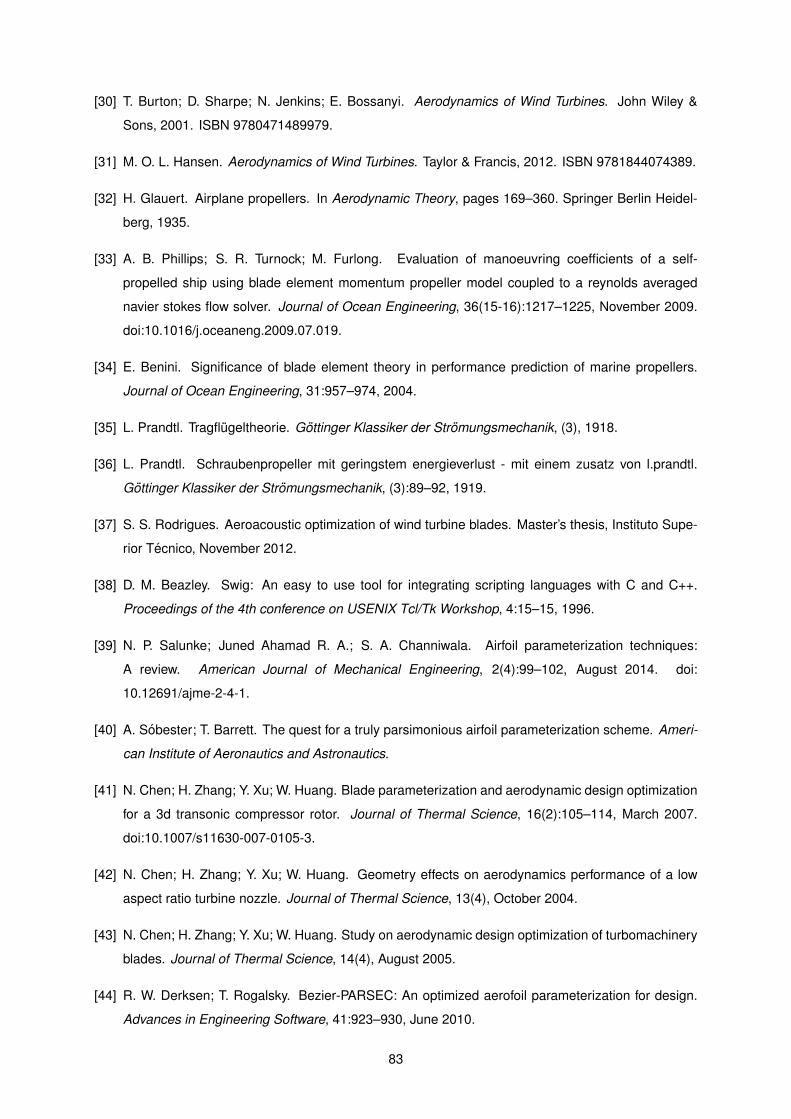
[30] T. Burton; D. Sharpe; N. Jenkins; E. Bossanyi. Aerodynamics of Wind Turbines. John Wiley &
Sons, 2001. ISBN 9780471489979.
[31] M. O. L. Hansen. Aerodynamics of Wind Turbines. Taylor & Francis, 2012. ISBN 9781844074389.
[32] H. Glauert. Airplane propellers. In Aerodynamic Theory, pages 169–360. Springer Berlin Heidel-
berg, 1935.
[33] A. B. Phillips; S. R. Turnock; M. Furlong. Evaluation of manoeuvring coefficients of a self-
propelled ship using blade element momentum propeller model coupled to a reynolds averaged
navier stokes flow solver. Journal of Ocean Engineering, 36(15-16):1217–1225, November 2009.
doi:10.1016/j.oceaneng.2009.07.019.
[34] E. Benini. Significance of blade element theory in performance prediction of marine propellers.
Journal of Ocean Engineering, 31:957–974, 2004.
[35] L. Prandtl. Tragflugeltheorie. Gottinger Klassiker der Stromungsmechanik, (3), 1918.
[36] L. Prandtl. Schraubenpropeller mit geringstem energieverlust - mit einem zusatz von l.prandtl.
Gottinger Klassiker der Stromungsmechanik, (3):89–92, 1919.
[37] S. S. Rodrigues. Aeroacoustic optimization of wind turbine blades. Master’s thesis, Instituto Supe-
rior Tecnico, November 2012.
[38] D. M. Beazley. Swig: An easy to use tool for integrating scripting languages with C and C++.
Proceedings of the 4th conference on USENIX Tcl/Tk Workshop, 4:15–15, 1996.
[39] N. P. Salunke; Juned Ahamad R. A.; S. A. Channiwala. Airfoil parameterization techniques:
A review. American Journal of Mechanical Engineering, 2(4):99–102, August 2014. doi:
10.12691/ajme-2-4-1.
[40] A. Sobester; T. Barrett. The quest for a truly parsimonious airfoil parameterization scheme. Ameri-
can Institute of Aeronautics and Astronautics.
[41] N. Chen; H. Zhang; Y. Xu; W. Huang. Blade parameterization and aerodynamic design optimization
for a 3d transonic compressor rotor. Journal of Thermal Science, 16(2):105–114, March 2007.
doi:10.1007/s11630-007-0105-3.
[42] N. Chen; H. Zhang; Y. Xu; W. Huang. Geometry effects on aerodynamics performance of a low
aspect ratio turbine nozzle. Journal of Thermal Science, 13(4), October 2004.
[43] N. Chen; H. Zhang; Y. Xu; W. Huang. Study on aerodynamic design optimization of turbomachinery
blades. Journal of Thermal Science, 14(4), August 2005.
[44] R. W. Derksen; T. Rogalsky. Bezier-PARSEC: An optimized aerofoil parameterization for design.
Advances in Engineering Software, 41:923–930, June 2010.
83
[45] T. A. Pastva. Bezier curve fitting. Master’s thesis, Naval Postgraduate School, Monterey, California,
September 1998.
[46] A. Marta. Multidisciplinary Design Optimization of Aircrafts. Class notes, Instituto Superior Tecnico,
2014.
[47] R. T. Marler; J. S. Arora. Survey of multi-objective optimization methods for engineering. Structures
and Multidisciplinary Optimization, 26:369–395, 2004. DOI: 10.1007/s00158-003-0368-6.
[48] K. Deb; A. Pratap; S. Agarwal; T. Meyarivan. A fast and elitist multiobjective genetic algorithm:
Nsga-ii. IEEE Transactions on Evolutionary Computation, 6(2):182–197, 2002.
[49] L. Wang; T. Wang; Y. Luo. Improved non-dominated sorting genetic algorithm (nsga)-ii in multi-
objective optimization studies of wind turbine blades. Applied Mathematics and Mechanics, 32(6):
739–748, 2011.
[50] R. E. Perez; P. W. Jansen; J. R. R. A. Martins. pyopt: A python-based object-oriented framework for
nonlinear constrained optimization. Structures and Multidisciplinary Optimization, 45(1):101–118,
2012. doi: 10.1007/s00158-011-0666-3.
[51] P. Moriarty; P. Migliore. Semi-empirical aeroacoustic noise prediction code for wind turbines. Tech-
nical Report NREL/TP-500-34478, National Renewable Energy Laboratory, December 2003.
84

Appendix A
Noise Prediction Models Equations
In this appendix, all of the equations that complete the models presented in chapter 2 are here defined,
as in [15].
A.1 TEB-VS
The spectral function G2 and all the required variables are defined as:
(G2)Ψ=14 =
mη + k (η < η0)
2.5
√1− (η/µ)
2 − 2.5 (η0 ≤ η < 0)√1.5625− 1194.99η2 − 1.25 (0 ≤ η < 0.03616)
−155.543η + 4.375 (0.03616 ≤ η)
(A.1)
η = log(St′′′/St
′′′peak
)(A.2)
µ =
0.1221 (h/δ∗avg < 0.25)
−0.2175 (h/δ∗avg) + 0.1755 (0.25 ≤ h/δ∗avg < 0.62)
−0.0308 (h/δ∗avg) + 0.0596 (0.62 ≤ h/δ∗avg < 1.15)
0.0242 (h/δ∗avg ≥ 1.15)
(A.3)
85

m =
0 (h/δ∗avg ≤ 0.02)
68.724 (h/δ∗avg)− 1.35 (0.02 < h/δ∗avg ≤ 0.5)
308.475 (h/δ∗avg)− 121.23 (0.5 < h/δ∗avg ≤ 0.62)
224.811 (h/δ∗avg)− 69.35 (0.62 < h/δ∗avg ≤ 1.15)
1583.28 (h/δ∗avg)− 1631.59 (1.15 < h/δ∗avg < 1.2)
268.344 (h/δ∗avg > 1.2)
(A.4)
η0 = −
√m2µ4
6.25 +m2µ2(A.5)
k = 2.5
√1−
(η0
µ
)2
− 2.5−mη0 (A.6)
The spectrum function (G2)Ψ=0 is obtained by computing equations (A.1) through (A.6) whilst re-
placing (h/δ∗avg) by (h/δ∗avg)′ where
(h
δ∗avg
)′= 6.724
(h
δ∗avg
)2
− 4.019
(h
δ∗avg
)+ 1.107 (A.7)
A.2 LBL-VS
The spectral shape function G3 is defined in terms of the ratio between the Strouhal number and its
peak,
G3(e) =
39.8 log(e)− 11.12 (e ≤ 0.5974)
98.409 log(e) + 2 (0.5974 < e ≤ 0.8545)
−5.076 +√
2.484− 506.25[log(e)]2 (0.8545 < e ≤ 1.17)
−98.409 log(e) + 2 (1.17 < e ≤ 1.674)
−39.8 log(e)− 11.12 (e > 1.674)
(A.8)
where e = St′/St′peak. The peak scaled level shape curve G4 is a function of the Reynolds number and it
is defined by
G4(e) =
77.852 log(d) + 15.328 (d ≤ 0.3237)
65.188 log(d) + 9.125 (0.3237 < d ≤ 0.5689)
−114.052[log(d)]2 (0.5689 < d ≤ 1.7579)
−65.188 log(d) + 9.125 (1.7579 < d ≤ 3.0889)
−77.852 log(d) + 15.328 (d > 3.0889)
(A.9)
86
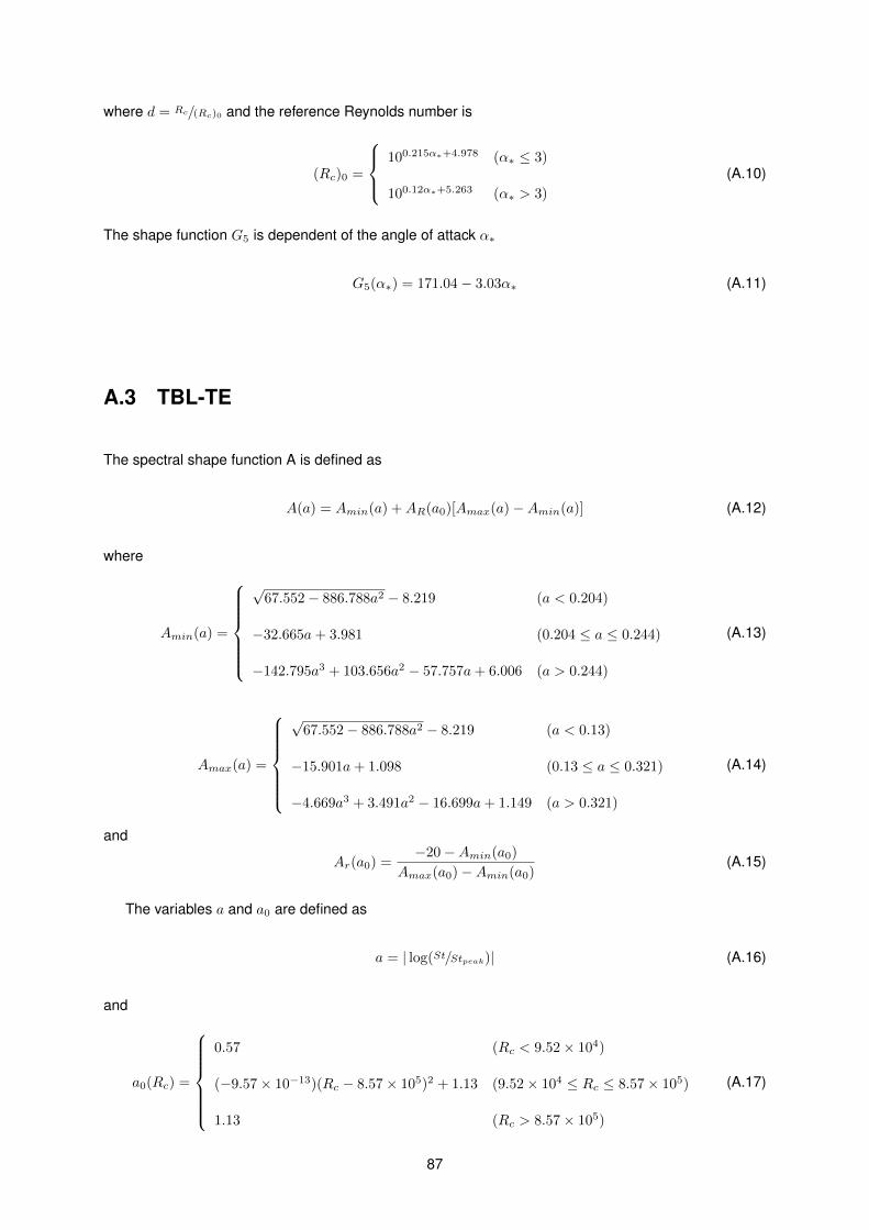
where d = Rc/(Rc)0 and the reference Reynolds number is
(Rc)0 =
100.215α∗+4.978 (α∗ ≤ 3)
100.12α∗+5.263 (α∗ > 3)
(A.10)
The shape function G5 is dependent of the angle of attack α∗
G5(α∗) = 171.04− 3.03α∗ (A.11)
A.3 TBL-TE
The spectral shape function A is defined as
A(a) = Amin(a) +AR(a0)[Amax(a)−Amin(a)] (A.12)
where
Amin(a) =
√67.552− 886.788a2 − 8.219 (a < 0.204)
−32.665a+ 3.981 (0.204 ≤ a ≤ 0.244)
−142.795a3 + 103.656a2 − 57.757a+ 6.006 (a > 0.244)
(A.13)
Amax(a) =
√67.552− 886.788a2 − 8.219 (a < 0.13)
−15.901a+ 1.098 (0.13 ≤ a ≤ 0.321)
−4.669a3 + 3.491a2 − 16.699a+ 1.149 (a > 0.321)
(A.14)
and
Ar(a0) =−20−Amin(a0)
Amax(a0)−Amin(a0)(A.15)
The variables a and a0 are defined as
a = | log(St/Stpeak)| (A.16)
and
a0(Rc) =
0.57 (Rc < 9.52× 10⁴)
(−9.57× 10⁻¹³)(Rc − 8.57× 10⁵)2 + 1.13 (9.52× 10⁴ ≤ Rc ≤ 8.57× 10⁵)
1.13 (Rc > 8.57× 10⁵)
(A.17)
87

In the same molds as A, the spectral shape function B is defined as
B(b) = Bmin(b) +BR(b0)[Bmax(b)−Bmin(b)] (A.18)
where
Bmin(b) =
√16.888− 886.788b2 − 4.109 (b < 0.13)
−83.607b+ 8.138 (0.13 ≤ b ≤ 0.145)
−817.81b3 + 355.21b2 − 135.024b+ 10.619 (a > 0.145)
(A.19)
Bmax(b) =
√16.888− 886.788b2 − 4.109 (b < 0.1)
−31.33b+ 1.854 (0.1 ≤ b ≤ 0.187)
−80.541b3 + 44.174b2 − 39.381b+ 2.344 (b > 0.187)
(A.20)
and
Br(b0) =−20−Bmin(b0)
Bmax(b0)−Bmin(b0)(A.21)
The variables b and b0 are defined as
a = | log(St/St2)| (A.22)
and
b0(Rc) =
0.3 (Rc < 9.52× 10⁴)
(−4.48× 10⁻¹³)(Rc − 8.57× 10⁵)2 + 0.56 (9.52× 10⁴ ≤ Rc ≤ 8.57× 10⁵)
0.56 (Rc > 8.57× 10⁵)
(A.23)
The amplitude function K1 is defined as
K1 =
−4.31 log(Rc) + 156.3 (Rc < 2.47× 10⁵)
−9 log(Rc) + 181.6 (2.47× 10⁵ ≤ Rc ≤ 8× 10⁵)
128.5 (Rc > 8× 10⁵)
(A.24)
and the correction for the pressure side contribution in nonzero angles of attack cases ∆K1 is given
by
∆K1 =
α∗[1.43 log(Rδ∗p )]− 5.29 (Rδ∗p ≤ 5000)
0 (Rδ∗p > 5000)
(A.25)
88

The amplitude function K2 is defined as
K2 = K1 +
−1000 (α∗ < γ0 − γ)√β2 − (β/γ)2(α∗ − γ0)2 + β0 (γ0 − γ ≤ α∗ ≤ γ0 + γ)
−12 (α∗ > γ0 + γ)
(A.26)
withγ = 27.094M + 3.31
γ0 = 23.43M + 4.561
β = 72.65M + 10.74
β0 = −34.19M − 13.82
(A.27)
89

90

Appendix B
Coordinate Systems
In this appendix, the transformation matrices between the various coordinate systems used in the aeroa-
coustic tool are defined.
Systems 1 and 2 are identical, being that the only difference between them is the position of their
origins, such that the distance between them equals the height of the location of the fan.
Since the shaft is assumed to be stiff, the transformation between system 2 and 3, given by trans-
formation matrix a23, consists only in a rotation about the z-axis with a magnitude of θrot, which is the
angle of rotation of the shaft:
a23 =
cos θrot sin θrot 0
− sin θrot cos θrot 0
0 0 1
(B.1)
System 4 has its origin in the hub of the rotor, and it is rotated about system 3 x-axis with the angle
θtwist, to account for the twist along the blade:
a34 =
1 0 0
0 cos θtwist sin θtwist
0 − sin θtwist cos θtwist
(B.2)
Therefore, to transform a vector in system 4 to system 1, the following transformation is applied,
along with the origin translations:
r1 = a32 · a43 · r5 (B.3)
or:
r1 = a23T · a43T · r5 (B.4)
91

92