1

Aerodynamics of the Quickie Aircraft Corporation (QAC) Q-200 and Tri-Q-200: Part 1 – Introduction/Modeling Basics

This is Part 1 (of 3) of a follow-up to my 2009 study discussing Q-2 decalage (Q-Talk 138). This study focuses on aerodynamic computer modeling of the Q-200 tandem wing configuration and comparison of those models with flying aircraft. -- Jay Scheevel, Grand Junction, Colorado

Introduction For many years I had a pet theory that the range of cruise and landing behavior observed in flying Q-200's were primarily the result of variations in relative incidence angles between the wing and canard (decalage angle). This led me to hands-on measurements the decalage of more than 20 flying Q-200’s or Tri-Q200’s over a number of years and an attempt to study the impact on performance of those same aircraft using informal data supplied by the pilots/owners. Those results were summarized in 2009 (in Q-Talk #138). I will not discuss that paper here, other than to say that once I finished that study, I still felt like I lacked sufficient quantitative answers that would allow me to make sense of the influence of decalage to the flight qualities of the Q-200. Also, around this time, I became more keenly focused on landing and take-off behavior of the Q-200 as preparation for (hopefully soon) test-flying my own Tri-Q200. In addition to the influence of decalage, I also wanted to know the contribution of other key variables such as gross-weight, center of gravity, and landing gear configuration particularly as it impacts landing and takeoff behavior.

In order to answer these remaining questions in a satisfactory way, I decided to numerically model the aerodynamics of the Q-200 and Tri-Q200 configurations. Others have attempted to analyze the Q-200 using PC-based “flight simulator” programs such as X-plane, but that approach only yields a simulated flight experience, the real value of which depends on one’s ability to translate the computerized flight experience to real life. I do not find much similarity between actual flight and any PC “simulators”, so I see no the direct value in using a flight simulator version of the Q-200 to try to answer my detailed questions. Also, I wanted some numbers to crunch, so I went in another direction, one that would also allow me to communicate useful information to other Q-200 enthusiasts.

I decided to use a “2D” aerodynamic numerical modeling tool based on the well-known X-foil “panel” approach. X-foil was developed years ago at MIT. X-foil has been reworked by Martin Hepperle into a comprehensive Java-based user interface called JavaFoil. JavaFoil incorporates analysis, graphical editing and custom interface tools that are very powerful and complementary to the numerical modeling routines. In addition, JavaFoil can model multiple, mutually interacting airfoils (so called “multifoils”). Javafoil has the option of modeling any configuration and also has the capability to simulate ground effect. JavaFoil can run scripts allowing automated repetition of experiments with changes to parameters such as decalage, elevator deflection, reflexor deflection or dynamic parameters such as Reynolds number, wing loading. The scripts allow me to re-run models any number of times to test sensitivity of single parameter changes. The use of scripts also limits the possibility of manual entry errors resulting from one-at-a-time runs. Javafoils capabilities align nicely with the modeling that I wished to perform on the tandem wing configuration of the Q2.

2D Panel methods like X-foil are insufficient to model true stall and post-stall behavior (they approximate this). A 2D panel method also does not model 3D flow (span wise flow and finite wing behavior). My analysis does not depend strongly on the details of stall behavior, because

2

the Q-200 main wing really never fully stalls and, as I will demonstrate, the canard normally cannot be forced into a full stall in the Q-200 configuration. So the modeling approximations of Javafoil are sufficient for my purposes. To approximate any 3D effects, I break down the Q wing into thirds and model them independently, then recombine the results in a spreadsheet with corrections added there. In this way I can handle washout (twist), sweep and span wise efficiency approximations. In summary, the JavaFoil platform has proven very adequate for my needs when combined with spreadsheet-hosted post-processing.

The spreadsheet is also where other calculations specific to the Q-200 geometry such as loading, and wing layout can be varied. Simplified non-wing drag moments (form, parasite, etc.) are introduced in spreadsheet calculations in order to achieve a match of the modeled performance to that of the entire flying aircraft with flight tests. All of the JavaFoil models and spreadsheet manipulations represent many tens of thousands of aerodynamic “experiments” on the virtual Q-200 “model”. Part 1 of this study (this section) is an introduction to the modeling procedure and unique considerations required to model the Q-200/Tri-Q200. Part 2 of this study is a summary of the Javafoil model results and how these results relate to take-off, landing, and level flight for various decalage values on the Q-200 and Tri-Q. Part 3 of this study is a review of flying aircraft from online videos and comparison of the Javafoil modeling results to actual flight behavior of those aircraft. The comparisons in Part 3 are done by dissecting photos and videos that have been posted on the internet by a number of Q pilot/owners. I use photos and performance data from the original QAC Q-200 prototype (N81QA) as well as photos and videos posted by Mike Dwyer (Q-200), Jerry Marstall (Tri-Q200), Sanjay Dall (Q-200) and Jean Paul Chevalier (Tri-Q200), all of whom have created nice point of view (POV) videos covering various facets of flight. My use of their videos IN NO WAY implies that any of these people have approved or any way endorsed any of my conclusions. Their videos are publicly available on the internet, so use of them to evaluate the validity of my modeling against actual flying Q-200’s or Tri-Q200’s is essentially use of public data.

I have chosen to present most of my conclusions graphically, so careful study of each graph, diagram and photograph along including its caption will aid the reader in the understanding of the parameters, model results and my conclusions.

DISCLAIMER: None of my results or conclusions should be taken as those generated by a trained aerodynamicist, which I in no way resemble. This study may provide qualitative insight into the unique flight characteristics of the Q-200 tandem wing configuration as well as the Tri-Q200 configuration during landing, take-off and level flight. Do not use any of this study’s results or conclusions to guide the building or test flying of any aircraft. This study is not advice for flight procedures for the Q-200 or Tri-Q200 unless you have personally and independently verified the results for yourself. This study has not been critically reviewed or verified so it cannot be regarded as scientifically reliable.

3

The JavaFoil Model JavaFoil requires a data file containing scaled coordinates of the airfoil(s) to be modeled. The Q-200 airfoil coordinates files were created by carefully digitizing original QAC Q-200 plan templates. To model the wing behavior, I divided each “wing” into roughly 1/3 (span wise) portions of more or less equal lengths, applying the appropriate template and dimensions for the central point of each third. The templates used for each 1/3 wing are positioned at the correct fuselage station (FS) and (water level) WL in order to approximate the layout of the Q-200. Each “third” is therefore consistent with the original Q-200 plan templates (LS-1 canard and Eppler main wing). Dividing the “wing” (i.e. wing and canard) into thirds incorporates the design elements of taper, sweep and washout (twist) of both canard and wing, and also allows for corrections to span efficiency. In this way, the model approximates the aerodynamic response of the total wing and canard.

JavaFoil computes the pressure and airflow on and around the canard and wing in true relative proximity, meaning that both flying surfaces interact dynamically within the same air mass. As such, each “third” contains both a canard and a wing section. I refer to these “thirds” as the inner, middle and outer thirds. To see the layout of all wing “thirds” for the zero decalage (e.g. “plans built”) configuration, refer to Figure 1. Note that there is no anhedral in the canard, since I am preferentially modeling the Tri-Q200. This said, several preliminary models containing anhedral (Q-200 conventional gear) reveal only very minor differences to the models with no anhedral. Consequently, I believe the modeling conclusions in this study are also as relevant to the Q-200 conventional gear layout as they are to the Tri-200 layout. This study addresses flight characteristics of both Q-200 and Tri-Q200 configurations.

Elevator deflections are limited to the inner two thirds of the canard to be consistent with elevator length and area. Reflexor deflections, where modeled, are limited to the inner one third of the main wing to be consistent with the aileron length and area. The modeled dimensions of the elevator and aileron compare favorably with their actual dimensions from the Q-200 plans. Control surface deflections in the model are limited to the same travel limits recommended by QAC Q-200 plans and templates.

Since the Q-200 fuselage is not modeled in JavaFoil, lift and induced drag computed in Javafoil are only those of the wing and canard. The model data is compiled in spreadsheets which allow the addition of parasitic and other non-wing drag moments and thrust forces, in order to calibrate the model performance to that of the actual QAC Q-200 prototype (N81QA) or flying Tri-Q200’s as required. Drag moment arm is varied as a function of alpha (AOA) in order to cause model airspeed and control deflections in level flight to match the detailed flight test data. Part 2 of this study details how the model is calibrated to test flights that were collected and reported in an 1983 article by Michael Huffman (posted on the Yahoo Q-list site, files section). N81QA is a tail dragger, so the drag moments are appropriate for that layout. Different moments and other considerations apply to the Tri-Q200 configuration.

For the purposes of this study, the canard level-line is defined as the “reference” alpha angle of zero degrees. Alpha is essentially equivalent to angle of attack for the purposes of this study. By definition a plans-built LS-1 canard has a level-line parallel to water line reference of the airframe. When in flight when the level line parallel to the relative wind, alpha is said to be at zero degrees.

Decalage angle is the angle of the main wings level line relative to the canard’s level line. A plans-built Q-200, by definition, would have a decalage angle of zero since the main wing is

4

installed with its level-line parallel to that of the canard and both main wing and canard level line parallel to the water level of the airframe. The decalage is varied for modeling purposes in this study.

It should be pointed out that the canard level-line may not necessarily be the “deck angle” of the aircraft (deck angle being synonymous with the water line). This is because the fuselage deck angle can vary from plane to plane depending on how the builder installs the canard and the wing relative to the fuselage water line. The deck angle of the fuselage does not significantly affect the aerodynamic contribution of the wings, but it does influence the non-wing drag distribution somewhat. The deck angle also plays a part in determining the landing gear position and ground angle of attack (taxi alpha) for both Q-200 and Tri-Q200 configurations as well as the pilots view over the nose. In a plans-built Q-200, the deck angle (water line) would ideally be parallel to the canard and wing level lines. However, I believe that QAC plan’s recommended methods for aligning all of these components (canard, wing, and fuselage) were insufficiently rigorous for the average builder to maintain precise tolerances. As a result, there are significant variations between all of these components in actual flying aircraft. This reality is why I chose to model a range of decalage angles in this study. For purposes of my study, the fuselage angle is considered to be the same as the QAC prototype (N81QA), the canard is parallel to that level line, and only the main wing angle is varied in my models in order to achieve different decalage values.

By this definition, if the main wing level-line is inclined “leading edge down” (relative to the canard), then the decalage is negative, and if the main wing level-line is inclined “leading edge up” (relative to the canard) then the decalage is positive. Again: Any alpha values in this study are referenced only to the canard. So the implied angle of incidence of the main wing is determined by adding the decalage value to the alpha value. This said, bear in mind that the canard and wing are interacting in the same air mass, and are of similar size and are relatively close to one another (aerodynamically speaking). Consequently, the downwash of the canard always reduces the effective alpha (relative wind) on the main wing (see Figure 2 and 3). The “effective” alpha/AOA of the main wing is lower than that experienced by the canard for all normal flight attitudes. This is why it is important to use a modeling approach that can model the two airfoils simultaneously and achieve accurate lift and induced drag behaviors for the combined canard-wing layout. This is especially important when in ground effect.

The Q-200 models in this study have decalage values ranging from plus 3 to minus 4 degrees (a total range of 7 degrees). This modeled range of decalage values is slightly larger than the actual range of values that I have measured over the years on actively flying Q-200’s or Tri-Q-200’s (see Q-talk 138). All of the Q’s that I have measured have significant total time and fly regularly, so they are presumably routinely controllable through all facets of flight despite their decalage variations.

The Q-200 design and aerodynamic modeling The strong interaction of canard and wing on the Quickie is unique because both the canard and wing are of similar span and chord dimensions. The Quickie configuration is unlike many of the more familiar Rutan canard designs (such as the Long-Eze or Vari-Eze) where the canard has significantly shorter span than the main wing, is much smaller in area, has a much smaller chord and a is a greater relative distance from the main wing. In these “-Eze” designs, even though there is considerably higher wing loading on the canard than on the main wing, the main wing still carries most of the gross weight. In contrast, the Quickie (and the Q-200) canard carries most of the gross weight (2/3 or more of the gross weight) has the same span and area

5

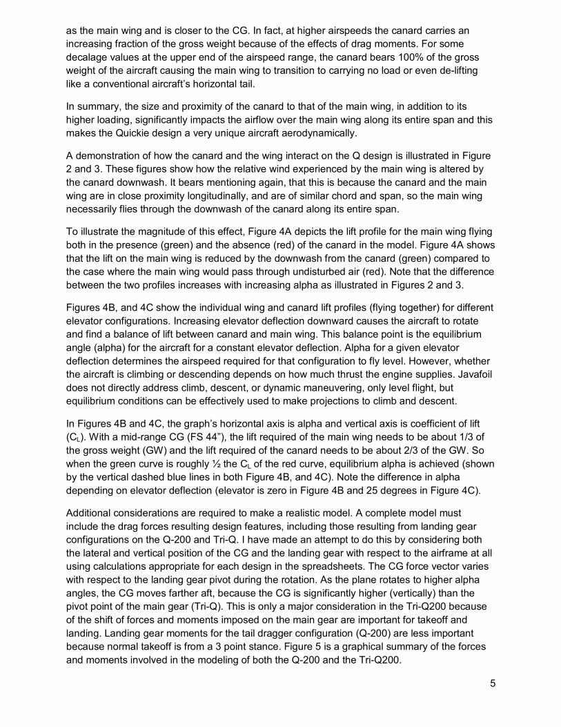
as the main wing and is closer to the CG. In fact, at higher airspeeds the canard carries an increasing fraction of the gross weight because of the effects of drag moments. For some decalage values at the upper end of the airspeed range, the canard bears 100% of the gross weight of the aircraft causing the main wing to transition to carrying no load or even de-lifting like a conventional aircraft’s horizontal tail.

In summary, the size and proximity of the canard to that of the main wing, in addition to its higher loading, significantly impacts the airflow over the main wing along its entire span and this makes the Quickie design a very unique aircraft aerodynamically.

A demonstration of how the canard and the wing interact on the Q design is illustrated in Figure 2 and 3. These figures show how the relative wind experienced by the main wing is altered by the canard downwash. It bears mentioning again, that this is because the canard and the main wing are in close proximity longitudinally, and are of similar chord and span, so the main wing necessarily flies through the downwash of the canard along its entire span.

To illustrate the magnitude of this effect, Figure 4A depicts the lift profile for the main wing flying both in the presence (green) and the absence (red) of the canard in the model. Figure 4A shows that the lift on the main wing is reduced by the downwash from the canard (green) compared to the case where the main wing would pass through undisturbed air (red). Note that the difference between the two profiles increases with increasing alpha as illustrated in Figures 2 and 3.

Figures 4B, and 4C show the individual wing and canard lift profiles (flying together) for different elevator configurations. Increasing elevator deflection downward causes the aircraft to rotate and find a balance of lift between canard and main wing. This balance point is the equilibrium angle (alpha) for the aircraft for a constant elevator deflection. Alpha for a given elevator deflection determines the airspeed required for that configuration to fly level. However, whether the aircraft is climbing or descending depends on how much thrust the engine supplies. Javafoil does not directly address climb, descent, or dynamic maneuvering, only level flight, but equilibrium conditions can be effectively used to make projections to climb and descent.

In Figures 4B and 4C, the graph’s horizontal axis is alpha and vertical axis is coefficient of lift (CL). With a mid-range CG (FS 44”), the lift required of the main wing needs to be about 1/3 of the gross weight (GW) and the lift required of the canard needs to be about 2/3 of the GW. So when the green curve is roughly ½ the CL of the red curve, equilibrium alpha is achieved (shown by the vertical dashed blue lines in both Figure 4B, and 4C). Note the difference in alpha depending on elevator deflection (elevator is zero in Figure 4B and 25 degrees in Figure 4C).

Additional considerations are required to make a realistic model. A complete model must include the drag forces resulting design features, including those resulting from landing gear configurations on the Q-200 and Tri-Q. I have made an attempt to do this by considering both the lateral and vertical position of the CG and the landing gear with respect to the airframe at all using calculations appropriate for each design in the spreadsheets. The CG force vector varies with respect to the landing gear pivot during the rotation. As the plane rotates to higher alpha angles, the CG moves farther aft, because the CG is significantly higher (vertically) than the pivot point of the main gear (Tri-Q). This is only a major consideration in the Tri-Q200 because of the shift of forces and moments imposed on the main gear are important for takeoff and landing. Landing gear moments for the tail dragger configuration (Q-200) are less important because normal takeoff is from a 3 point stance. Figure 5 is a graphical summary of the forces and moments involved in the modeling of both the Q-200 and the Tri-Q200.

6

Figure 6 is a graphical representation of the relative position of the force vectors such as CG, and the canard and wing centers of lift as a function of rotation angle. The vertical red is the fixed Tri-Q200 main gear location (FS, fuselage station 56.5”). The blue lines show the relative positions of the center of pressure for each wing and the green line represents the relative position of the CG as the airframe rotates on the main gear to higher values of alpha.

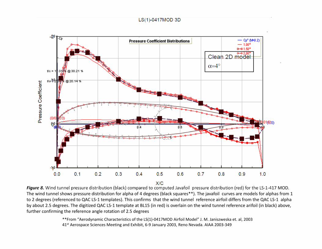
Validation of Javafoil Pressure Distributions to Wind Tunnel Models Whenever possible, numerical models should be compared to actual wind tunnel testing for validation. Fortunately, extensive modern wind tunnel testing of the LS(1)-0417MOD airfoil has been performed at Ohio State University using Reynolds numbers near 1 million, which are appropriate for the flight regime of the Q-200. This wind tunnel test data** allows a direct comparison of wind tunnel measured lift, drag and pressure distributions to from Javafoil (shown in Figures 10 and 11). The wind tunnel and Javafoil results compare favorably, but it appears that the QAC LS-1 airfoil template at BL15 has a “reference” level-line that differs from that of the standard NASA LS(1)-0417MOD by about 2.5 degrees. Since my study is referenced to the QAC plans template-angle, it is appropriate to shift the Javafoil curve by 2.5 degrees for comparison to the wind tunnel data, making the level reference the same for comparison purposes. When this correction is done, both the lift profile and the pressure distribution from Javafoil match very closely to the wind tunnel measurements at all alphas up to the point of full stall. I was unable to find wind tunnel tests of the Eppler 1212 (Q-200 main wing) airfoil, but the good comparison between the LS-1 Javafoil model and actual wind tunnel results provides confidence in the validity of the Javafoil computational engine.

End of Part 1.

Figure 1. Typical JavaFoil model wing sections. All three “thirds” are superimposed in this figure,however each third is modelled independently and then JavaFoil output is combined in aspreadsheet for analysis. The red “Pivot” label at the bottom is the contact point of the main gearwith the runway for the Tri‐Q200 configuration and is located at FS 56.5 when the aircraft ishorizontal. The horizontal blue line is the runway surface. The vertical offset of the main wingsections are the result of wing dihedral (also note the washout). The Tri‐Q200 LS‐1 canard is builtwithout anhedral, so the “thirds” sections plot on top of one another in this view. The vertical blueline is the location of the firewall (FS 14).

Alpha=0 degrees (plans built)No Ground Effect

Figure 2. Streamlines for airflow over plans‐built Q‐200 with LS‐1 Canard, flying at Alpha=0 (Re~ 10 E6). Red arrows approximate the angle of relative wind for each airfoil. Note that there is some downwash from the canard, even at small Alphas, causing the main wing to “see” a lower effective Alpha.

Figure 3. Streamlines for “plans‐built” Q‐2 with LS‐1 Canard, flying at Alpha=8 degrees (Re~ 10 E6). Elevator is 25 degrees . Red arrows are the approximate angle of relative wind for each airfoil (inner third). There is significant downwash from the canard at this Alpha, causing the main wing to “see” a much lower effective Alpha than the canard experiences. The effective relative wind on the wing is ~3 degrees lower than the canard.

Alpha=8 degrees (plans built)No Ground Effect

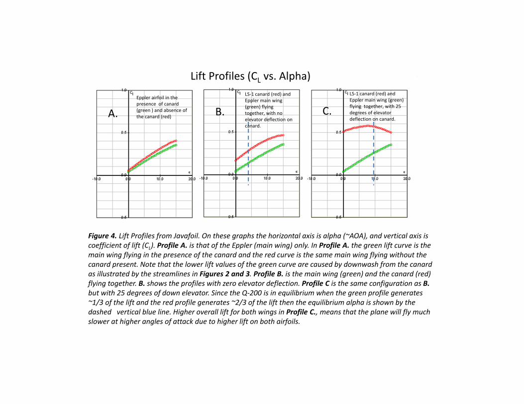
Figure 4. Lift Profiles from Javafoil. On these graphs the horizontal axis is alpha (~AOA), and vertical axis is coefficient of lift (CL). Profile A. is that of the Eppler (main wing) only. In Profile A. the green lift curve is the main wing flying in the presence of the canard and the red curve is the same main wing flying without the canard present. Note that the lower lift values of the green curve are caused by downwash from the canard as illustrated by the streamlines in Figures 2 and 3. Profile B. is the main wing (green) and the canard (red) flying together. B. shows the profiles with zero elevator deflection. Profile C is the same configuration as B.but with 25 degrees of down elevator. Since the Q‐200 is in equilibrium when the green profile generates ~1/3 of the lift and the red profile generates ~2/3 of the lift then the equilibrium alpha is shown by the dashed   vertical blue line. Higher overall lift for both wings in Profile C., means that the plane will fly much slower at higher angles of attack due to higher lift on both airfoils. 

A. B. C.Eppler airfoil in the presence  of canard (green ) and absence of the canard (red)

LS‐1 canard (red) and Eppler main wing (green) flying  together, with no elevator deflection on canard.

LS‐1 canard (red) and Eppler main wing (green) flying  together, with 25 degrees of elevator deflection on canard.

Lift Profiles (CL vs. Alpha)

Moments relative to FS 44 (mid range CG)A. Main Gear:  +12.5 in. (aft of level CG)B. Nose Gear:  ‐35 in. (forward of CG)C. Canard lift/drag:  approx.  ‐24 in. (forward of CG)D. MW lift/drag:  approx. +40 in. (aft of CG)E. Thrust F. non‐lift drag/arm (AOA dependent)

Sign conventions:Lift arms are positive when aft of and negative when forward of CG.

Forces are negative upward and positive downwardResulting moments are positive clockwise (increasing alpha (~AOA)) and 

negative counterclockwise (decreasing alpha)Deck angle and alpha are only equal when in level flight on per‐plans A/C.

A

B

C

D

Tri‐Q200 (Q‐200) Lift, Drag, Weight & Thrust Moments/Arms 

Figure 5.Weight and Lift forces and moment arms with respect to the CG. C and D are the lift and drag forces canard and wing respectively. Once in flight, these are the same for both Q‐200 and Tri‐Q200 (A, and B forces vanish once airborne).

EF

Tri-Q200 Centers of Pressure (blue) of W ing and Canard with respect to the Main Gear axle (red) and CG (green)

from 0 to 15 Alpha (angle of attack)(plans-built MW and Canard incidences. C.P.'s are mid-wing)

Fuselage Station (inches)

20 30 40 50 60 70 80 90 100 110

Alp

ha (d

egre

es)

0123456789

101112131415

Eppler-Main W ing and LS1-Canard C.P.'s FS main gear axle (FS 56.5)CG (FS 45) vs Alpha

Figure 6. The chart shows the position of the centers of pressure for both the canard (left blue curve) and the main wing (right blue curve), relative to fuselage station (FS) fixed to the pivot point of the main landing gear on the Tri‐Q200 (red curve @ FS 56.5”). The green curve shows how a CG located at FS45 moves aft with increasing rotation. Note that if the plane is rotated much past ~16 degrees, the CG would move aft of the main gear pivot and the plane would fall on its tail.

Figure 7. Wind tunnel lift profile (black) compared to Javafoil QAC LS1 template profile for the inner 1/3 span of canard (green).Thewind tunnel lift profile departs from linear at ~8.5 degrees achieving a full stall at ~15.5 degrees. The javafoil LS1 is shifted ‐2.5 degrees to align with the wind tunnel data, so departs from linear at 6 degrees (relative to QAC template level line), and is fully stalled at 13 degrees. The inner 1/3 of the LS‐1 canard of the plans built QAC canard is about 2.5 degrees high to the NASA reference LS‐1‐417 MOD airfoil used in the wind tunnel studies. This is consistent with the pressure distribution shown in Figure 8.

**From “Aerodynamic Characteristics of the LS(1)‐0417MOD Airfoil Model” J. M. Janiszweska et. al, 200341st Aerospace Sciences Meeting and Exhibit, 6‐9 January 2003, Reno Nevada. AIAA 2003‐349

**From “Aerodynamic Characteristics of the LS(1)‐0417MOD Airfoil Model” J. M. Janiszweska et. al, 200341st Aerospace Sciences Meeting and Exhibit, 6‐9 January 2003, Reno Nevada. AIAA 2003‐349

Figure 8. Wind tunnel pressure distribution (black) compared to computed Javafoil pressure distribution (red) for the LS‐1‐417 MOD. The wind tunnel shows pressure distribution for alpha of 4 degrees (black squares**). The javafoil curves are models for alphas from 1 to 2 degrees (referenced to QAC LS‐1 templates). This confirms  that the wind tunnel  reference airfoil differs from the QAC LS‐1  alpha by about 2.5 degrees. The digitized QAC LS‐1 template at BL15 (in red) is overlain on the wind tunnel reference arifoil (in black) above, further confirming the reference angle rotation of 2.5 degrees