aeroelastic ground wind loads analysis tool for launch ... · pdf fileaeroelastic ground wind...
TRANSCRIPT

American Institute of Aeronautics and Astronautics
1
Aeroelastic Ground Wind Loads Analysis Tool for Launch
Vehicles
Thomas G. Ivanco1
NASA Langley Research Center, Hampton, VA, 23681
Launch vehicles are exposed to ground winds during rollout and on the launch pad that
can induce static and dynamic loads. Of particular concern are the dynamic loads caused by
vortex shedding from nearly-cylindrical structures. When the frequency of vortex shedding
nears that of a lowly-damped structural mode, the dynamic loads can be more than an order
of magnitude greater than mean drag loads. Accurately predicting vehicle response to vortex
shedding during the design and analysis cycles is difficult and typically exceeds the practical
capabilities of modern computational fluid dynamics codes. Therefore, mitigating the ground
wind loads risk typically requires wind-tunnel tests of dynamically-scaled models that are time
consuming and expensive to conduct. In recent years, NASA has developed a ground wind
loads analysis tool for launch vehicles to fill this analytical capability gap in order to provide
predictions for prelaunch static and dynamic loads. This paper includes a background of the
ground wind loads problem and the current state-of-the-art. It then discusses the history and
significance of the analysis tool and the methodology used to develop it. Finally, results of the
analysis tool are compared to wind-tunnel and full-scale data of various geometries and
Reynolds numbers.
Nomenclature
CD = drag coefficient
CDp = dynamic drag coefficient
�̃�𝐿𝑜 = standard deviation of the lift coefficient for a rigid structure in smooth flow
�̃�𝐿𝑟 = resulting standard deviation of the lift coefficient for a rigid structure (smooth or turbulent)
�̃�𝐿 = resulting standard deviation of the lift coefficient for a flexible structure
CLm = increase factor to the standard deviation of the lift coefficient as a result of structural motion
(CLm = �̃�𝐿/�̃�𝐿𝑟)
D = cylinder diameter
dS = bandwidth parameter of the power spectral density (PSD) of oscillating lift for smooth flow
dB = resulting bandwidth parameter of the PSD for turbulent flow
fh = structural frequency (Hz)
fns = natural vortex shedding frequency (Hz)
Iu = turbulence content of the approaching flow, standard deviation of the along-wind velocity normalized
by the mean along-wind velocity
LC = correlation length of vortex shedding on a three-dimensional structure
Re = Reynolds number
St = Strouhal number (fnsD/V)
ζ = structural damping ratio with respect to critical damping
I. Introduction
AUNCH vehicles are exposed to ground winds during rollout and on the pad prior to launch that can induce static
and dynamic loads in the vehicle structure. The study of these loads is often referred to as ground wind loads
(GWL) and has been the topic of many wind-tunnel tests and technical reports.1-16
1 Research Aerospace Engineer, Aeroelasticity Branch, Mail Stop 340, AIAA Senior Member.
L
https://ntrs.nasa.gov/search.jsp?R=20160007745 2018-05-11T19:15:11+00:00Z

American Institute of Aeronautics and Astronautics
2
A comprehensive background into the GWL problem with respect to launch vehicles is presented in Refs. 1 and
2. In summary, the atmospheric winds can be comprised of mean winds with a boundary-layer profile, atmospheric
gusts and turbulence, and the turbulent wake of nearby structures. The launch vehicle structure (or wind-tunnel model)
experiences a response and accompanying loads that can be categorized as static and dynamic with components
resolved in the parallel (drag) and orthogonal (lift) directions with respect to the wind. The dynamic response of the
structure can be the result of flow perturbations or the result of vortex shedding. Of particular concern is the dynamic
structural response due to vortex shedding when a Kármán vortex street forms in the wake of the structure resulting
in nearly sinusoidal lift and drag forces. This response is termed wind-induced oscillation (WIO). When the frequency
of vortex shedding approaches that of a structural mode and there is insufficient damping to dissipate those loads, the
dynamic response of the structure can become very large and dynamic loads can be more than an order of magnitude
greater than the loads induced by drag. A dynamic response of this nature is referred to as resonant WIO. In certain
cases of resonant WIO response, the shedding frequency departs from its natural frequency and occurs at the structural
frequency. This shift in the natural shedding frequency is termed “lock-in.” When the vortex shedding frequencies are
not close to a structural mode, there could still be a notable structural response (especially in a turbulent atmosphere),
and a response of this nature is referred to as non-resonant WIO response.
Material stresses that result from bending moments typically far exceed those resulting from shear forces for the
GWL problem. Therefore, base bending moments are typically presented to express the structural response to lift and
drag forces. It is important to note that the base of the structure may not contain the highest loads when higher modes
(second bending and beyond) are excited. Ref. 2 presents data for the Ares I-X GWL and buffet wind-tunnel tests and
analyses. As shown in Ref. 2, second mode GWL response can produce higher loads in the center region of the vehicle
(near the anti-node) than those generated by transonic buffet during ascent as a result of the load distribution associated
with a second mode response.
This paper describes a GWL analysis tool for launch vehicles that was recently developed by NASA. Beginning
with a brief background on the GWL problem, this paper will discuss the current state-of-the-art with respect to ground
wind loads analysis and testing efforts highlighting the need for the analysis tool presented here. The analysis tool will
be introduced including its history, its methodology, the pertinent equations, its current ability, and the planned future
efforts. Finally, a comparison of the analysis tool results to wind-tunnel and full-scale data is presented.
II. Current State-of-the-Art
Recent NASA efforts to examine GWL include those done for the Constellation Program and for the Space Launch
System (SLS) program. Constellation was the NASA human space flight program from 2005 through 2009 and
incorporated an “Ares I” launch vehicle for human crew and an “Ares V” launch vehicle for cargo. SLS is the current
NASA vehicle concept for human exploration and leverages the lessons learned from the Constellation Program. In
the recent NASA studies of launch vehicle GWL, there were four methods employed:
1) Using the initial design guidance of NASA SP-8008, Prelaunch Ground Wind Loads.3 The limitations of
this method are that it is NOT a load predictor, but rather serves as guidance for providing design margin.
Additionally, it is not mentioned in the publication, but this method relies on an assumption that vehicle
damping will be adequate to prevent large resonant WIO response.
2) Conducting a wind-tunnel test of an aeroelastically-scaled model. Some limitations of this method are that
it is expensive, it requires a lot of design and fabrication efforts, the wind-tunnel may not be able to
simulate all desired conditions, flow properties, or vehicle properties, and the results are often available
too late to make cost-effective design changes.
3) Conducting an analysis using empirical data. The limitations of this method are that different analyses can
produce wildly different results and developers must often anchor their predictions upon coefficients
derived experimentally from models representative of their vehicle.
4) Using physics-based Computational Fluid Dynamics (CFD) codes. The limitations of this method are that
it is difficult for modern CFD to model the separation location and resulting shed vortex with appropriate
accuracy and reliability with a practical mesh size. Additionally, the characterization of a launch vehicle
using CFD would likely require the analysis of thousands of conditions making high-order CFD simulation
unpractical.
GWL efforts for the Ares launch vehicles included multiple analyses and two aeroelastic wind-tunnel tests
comprising all four of the above methods. Additional details explaining the limitations of the four state-of-the-art
methods follow.

American Institute of Aeronautics and Astronautics
3
The initial design guidance of Ref. 3 was used to determine that the base of the Ares vehicles likely provided
adequate strength. However, this design guidance is incapable of modeling peak response conditions or magnitudes.
As expected, resonant WIO conditions in the wind tunnel resulted in dynamic loads more than an order of magnitude
higher than the initial design guidance would suggest.
The first of two Ares wind-tunnel tests was of a research “Checkout Model” similar geometrically and dynamically
to the early Ares I design.1,2 The second GWL wind-tunnel test was of the Ares I-X flight test vehicle (FTV), a later
version of the Ares I design.1,2 To distinguish between model-scale and full-scale, this paper will use FTV to
differentiate the full-scale vehicle from the wind-tunnel model of the Ares I-X. Both wind-tunnel tests were conducted
in the NASA Langley Transonic Dynamics Tunnel (TDT), and the results have been published in various program
reports, an AIAA conference paper, and journal article.1,2 The latter publication in the AIAA Journal of Spacecraft
and Rockets also includes a comparison of the Ares I-X FTV data to that of the TDT data. Consistent with previous
findings from the Jupiter and Scout programs,4,5 the FTV experienced cross-wind (lift direction) dynamics that were
a factor of two above those predicted in the wind tunnel with smooth uniform flow for non-resonant WIO response.
Figure 1 contains a comparison of the Ares I-X FTV data with Ares I-X wind-tunnel data for similar flow speed and
azimuth angle.
Semi-empirical GWL analyses were done of the Ares I-X FTV and are referred to, herein, as the “analysis used
for design” since they were the sanctioned loads used during design analysis cycles. These computations included
steady drag and an estimated response due to gusts in addition to a prediction of the WIO response. If one were to
analyze only the WIO component of the analysis used for design, there was very little predicted response at any
condition and variations in Strouhal number and other parameters had little effect. However, history reveals that a
resonant WIO response can be very large, and it is very sensitive to changes in Strouhal number and other
characteristics.1-16 The WIO component of the analysis used for design is also included in Fig. 1 for the same wind
conditions as those experienced by the FTV for the non-resonant WIO response. Correlation with a resonant WIO
response would likely have been much worse. As a result of this analysis, the Ares I-X FTV was rolled out without
stabilization or damping, and it was not until
after the acquisition of experimental results
that the need for a stay damper was
considered for extended pad stay. The late
realization that damping would be required
for Ares I-X led to a rushed design and
construction effort.
Intentionally very similar in geometry
and frequencies to the Ares I-X was the Ares
I crew launch vehicle (CLV). Ares I CLV
GWL analyses were also conducted using a
semi-empirical method that was different
from the method employed for the Ares I-X,
and it used conservative assumptions. The
results of the Ares I CLV method predicted
such a strong response to GWL that the vehicle was designed to have a T-0 damper (a damper that is attached until
main engine start). This vastly different result for two very similar vehicles highlights the uncertainty in using
traditional empirical methods that are not anchored in experimentally-determined coefficients from the design in
question.
Checkout Model GWL computations were performed using the unstructured-grid Navier Stokes CFD code
FUN3D.17 Reynolds numbers of the Checkout Model were in the vicinity of 1x10⁶ to 5x10⁶, based upon upper stage
diameter, and this range matched those of an equivalent full-scale vehicle. Both rigid and flexible vehicle simulations
were performed with a 3.3 x10⁶ node grid of the complete model. The grid size and turbulence model used were
inadequate to accurately simulate the peak vortex shedding loads in this Reynolds number range.18 However, the
numerous computations required for the various wind conditions seen by the vehicle made a much denser mesh
impractical. As might be expected, the turbulent simulations produced a bending moment and vehicle motion that
were too low in comparison with the wind-tunnel data. CFD simulations with a laminar boundary layer showed better
correlation, but were still substantially low in predicting a resonant WIO response. Fig. 2 contains data comparing the
wind-tunnel and CFD results of the Checkout Model for the same conditions of wind azimuth and speed. Additional
rigid computations were performed with a mesh on the order of 20 times larger, and only for the upper stage of the
vehicle.19 The Detached Eddy Simulation turbulence model was used, and these results indicate a vortex shedding
with much richer spectral content. Unfortunately, computing resources were significant for this rigid simulation that
Figure 1. Peak amplitude comparison of analysis used for design,
wind-tunnel data, and full-scale data, Ares I-X.
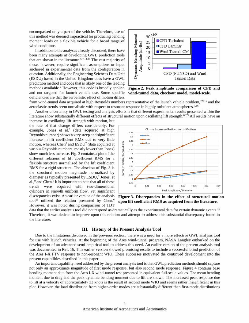
American Institute of Aeronautics and Astronautics
4
encompassed only a part of the vehicle. Therefore, use of
this method was deemed impractical for producing bending
moment loads on a flexible vehicle for a broad range of
wind conditions.
In addition to the analyses already discussed, there have
been many attempts at developing GWL prediction tools
that are shown in the literature.6,7,14,16 The vast majority of
these, however, require significant assumptions or input
anchored in experimental data from the configuration in
question. Additionally, the Engineering Sciences Data Unit
(ESDU) based in the United Kingdom does have a GWL
prediction method and code that is likely one of the leading
methods available.7 However, this code is broadly applied
and not targeted for launch vehicle use. Some specific
deficiencies are that the aeroelastic effect of motion differs
from wind-tunnel data acquired at high Reynolds numbers representative of the launch vehicle problem,7,9,16 and the
aeroelastic trends seem unrealistic with respect to resonant response in highly turbulent atmospheres.7,16
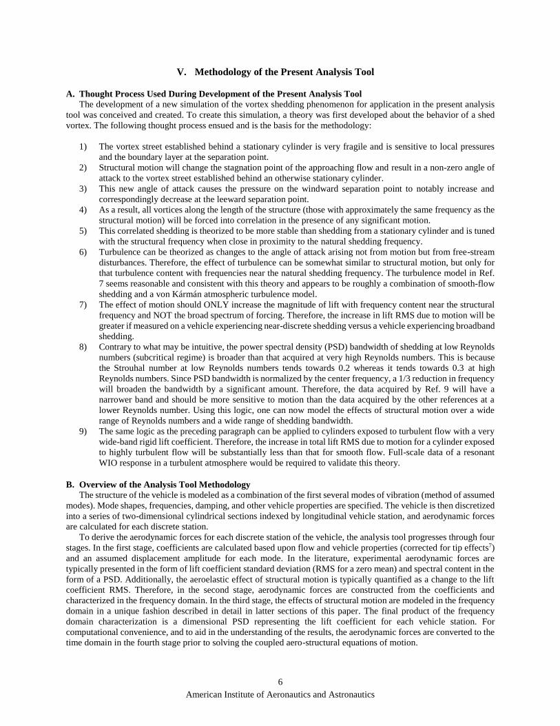
Another uncertainty in GWL testing and analysis efforts is that different experimental results presented within the
literature show substantially different effects of structural motion upon oscillating lift strength.6,7,9 All results have an
increase in oscillating lift strength with motion, but
the rate of that change differs considerably. For
example, Jones et al.9 (data acquired at high
Reynolds number) shows a very steep and significant
increase in lift coefficient RMS due to very little
motion, whereas Chen6 and ESDU7 (data acquired at
various Reynolds numbers, mostly lower than Jones)
show much less increase. Fig. 3 contains a plot of the
different relations of lift coefficient RMS for a
flexible structure normalized by the lift coefficient
RMS for a rigid structure. The abscissa of Fig. 3 is
the structural motion magnitude normalized by
diameter as typically presented by ESDU,7 Jones, et
al.,9 and Chen.6 It is important to note that all of these
trends were acquired with two-dimensional
cylinders in smooth uniform flow, yet significant
discrepancies exist. An earlier version of the analysis
tool16 utilized the relation presented by Chen.6
However, it was noted during comparison of TDT
data that the earlier analysis tool did not respond as dramatically as the experimental data for certain dynamic events.16
Therefore, it was desired to improve upon this relation and attempt to address this substantial discrepancy found in
the literature.
III. History of the Present Analysis Tool
Due to the limitations discussed in the previous section, there was a need for a more effective GWL analysis tool
for use with launch vehicles. At the beginning of the Ares wind-tunnel program, NASA Langley embarked on the
development of an advanced semi-empirical tool to address this need. An earlier version of the present analysis tool
was documented in Ref. 16. This earlier version showed promising results to include a successful blind prediction of
the Ares I-X FTV response to non-resonant WIO. These successes motivated the continued development into the
present capabilities described in this paper.
An important capability need addressed by the present analysis tool is that GWL prediction methods should capture
not only an approximate magnitude of first mode response, but also second mode response. Figure 4 contains base
bending moment data from the Ares I-X wind-tunnel test presented in equivalent full-scale values. The mean bending
moment due to drag and the peak dynamic bending moment due to lift are shown. The increased peak response due
to lift at a velocity of approximately 33 knots is the result of second mode WIO and seems rather insignificant in this
plot. However, the load distribution from higher-order modes are substantially different than first-mode distributions
Figure 2. Peak amplitude comparison of CFD and
wind-tunnel data, checkout model, model-scale.
Figure 3. Discrepancies in the effect of structural motion
upon lift coefficient RMS as acquired from the literature.

American Institute of Aeronautics and Astronautics
5
and may not be the largest at the base where
ground wind loads are typically measured. Figure
5 contains data from the same experiment as Fig.
4, however, it is resolved about the vehicle station
where the second mode anti-node exists. Finite
Element Model (FEM) analysis was used to
derive the corresponding loads at the anti-node as
a result of the different modal contributions. The
loads shown in Fig. 5 are dynamic three-sigma
values (three times the standard deviation) of the
modal components due to lift, and the mean value
due to drag. At this vehicle station, the second
mode peak at 33 knots not only produced the
highest dynamic loads, but it also occurred where
the drag loads and first mode response also
produce significant loads. Furthermore, the
vehicle strength at the anti-node is substantially
less than the vehicle base. As a result, second
mode WIO response measured in the wind tunnel
at this and other conditions exceed the peak loads
derived from the combined ascent loads analysis2
and therefore, could result in the most critical
loading condition for the Ares I-X.
IV. Significance and Applicability of the Present Analysis Tool
The present analysis tool is an advanced semi-empirical method that fills the analysis capability gap within the
state-of-the-art. Unlike other empirical methods,6,14 the present analysis tool is of general form and applicable to any
single-body design of nearly cylindrical shape. The effect of wake from adjacent structures can be estimated for
broadband wake typical of truss-like structures; however, multi-body simulation is beyond the scope of the analysis
tool.
The acquisition of coefficients from experiments using models similar in design to the vehicle in question is not
required. All results of the present analysis tool presented in this paper were generated by the same code with the only
changes for various results being dictated by user-defined input parameters. These input parameters specify vehicle
characteristics and the flow conditions being simulated. Vehicle characteristics are determined by design choices and
FEM analysis. Guidance regarding typical atmospheric conditions and design recommendations are provided by
climatic guidelines20 and space vehicle design criteria.3 It is recommended to investigate a wide range of wind profiles
and velocities during vehicle design analysis cycles in order to identify wind conditions that could produce significant
dynamic response.
Finally, it is important to note that tuning of the results to match a particular data set presented in this paper was
not conducted. Rather, the methodology described in this paper, anchored in the data from Ref. 9 that is the most
applicable to the launch vehicle problem, was applied generally across all simulations.
Figure 4. Wind-tunnel data in equivalent full-scale values, mean
drag and peak due to lift, Ares I-X.
Figure 5. Evaluation of loads at the second-mode anti-node,
modal contributions derived from wind-tunnel data, Ares I-X.
American Institute of Aeronautics and Astronautics
6
V. Methodology of the Present Analysis Tool
A. Thought Process Used During Development of the Present Analysis Tool
The development of a new simulation of the vortex shedding phenomenon for application in the present analysis
tool was conceived and created. To create this simulation, a theory was first developed about the behavior of a shed
vortex. The following thought process ensued and is the basis for the methodology:
1) The vortex street established behind a stationary cylinder is very fragile and is sensitive to local pressures
and the boundary layer at the separation point.
2) Structural motion will change the stagnation point of the approaching flow and result in a non-zero angle of
attack to the vortex street established behind an otherwise stationary cylinder.
3) This new angle of attack causes the pressure on the windward separation point to notably increase and
correspondingly decrease at the leeward separation point.
4) As a result, all vortices along the length of the structure (those with approximately the same frequency as the
structural motion) will be forced into correlation in the presence of any significant motion.
5) This correlated shedding is theorized to be more stable than shedding from a stationary cylinder and is tuned
with the structural frequency when close in proximity to the natural shedding frequency.
6) Turbulence can be theorized as changes to the angle of attack arising not from motion but from free-stream
disturbances. Therefore, the effect of turbulence can be somewhat similar to structural motion, but only for
that turbulence content with frequencies near the natural shedding frequency. The turbulence model in Ref.
7 seems reasonable and consistent with this theory and appears to be roughly a combination of smooth-flow
shedding and a von Kármán atmospheric turbulence model.
7) The effect of motion should ONLY increase the magnitude of lift with frequency content near the structural
frequency and NOT the broad spectrum of forcing. Therefore, the increase in lift RMS due to motion will be
greater if measured on a vehicle experiencing near-discrete shedding versus a vehicle experiencing broadband
shedding.
8) Contrary to what may be intuitive, the power spectral density (PSD) bandwidth of shedding at low Reynolds
numbers (subcritical regime) is broader than that acquired at very high Reynolds numbers. This is because
the Strouhal number at low Reynolds numbers tends towards 0.2 whereas it tends towards 0.3 at high
Reynolds numbers. Since PSD bandwidth is normalized by the center frequency, a 1/3 reduction in frequency
will broaden the bandwidth by a significant amount. Therefore, the data acquired by Ref. 9 will have a
narrower band and should be more sensitive to motion than the data acquired by the other references at a
lower Reynolds number. Using this logic, one can now model the effects of structural motion over a wide
range of Reynolds numbers and a wide range of shedding bandwidth.
9) The same logic as the preceding paragraph can be applied to cylinders exposed to turbulent flow with a very
wide-band rigid lift coefficient. Therefore, the increase in total lift RMS due to motion for a cylinder exposed
to highly turbulent flow will be substantially less than that for smooth flow. Full-scale data of a resonant
WIO response in a turbulent atmosphere would be required to validate this theory.
B. Overview of the Analysis Tool Methodology
The structure of the vehicle is modeled as a combination of the first several modes of vibration (method of assumed
modes). Mode shapes, frequencies, damping, and other vehicle properties are specified. The vehicle is then discretized
into a series of two-dimensional cylindrical sections indexed by longitudinal vehicle station, and aerodynamic forces
are calculated for each discrete station.
To derive the aerodynamic forces for each discrete station of the vehicle, the analysis tool progresses through four
stages. In the first stage, coefficients are calculated based upon flow and vehicle properties (corrected for tip effects7)
and an assumed displacement amplitude for each mode. In the literature, experimental aerodynamic forces are
typically presented in the form of lift coefficient standard deviation (RMS for a zero mean) and spectral content in the
form of a PSD. Additionally, the aeroelastic effect of structural motion is typically quantified as a change to the lift
coefficient RMS. Therefore, in the second stage, aerodynamic forces are constructed from the coefficients and
characterized in the frequency domain. In the third stage, the effects of structural motion are modeled in the frequency
domain in a unique fashion described in detail in latter sections of this paper. The final product of the frequency
domain characterization is a dimensional PSD representing the lift coefficient for each vehicle station. For
computational convenience, and to aid in the understanding of the results, the aerodynamic forces are converted to the
time domain in the fourth stage prior to solving the coupled aero-structural equations of motion.

American Institute of Aeronautics and Astronautics
7
At the conclusion of the four stages, the process is repeated for each station of the vehicle until time-domain forces
are determined for the full length of the vehicle. These full-length forces are then multiplied by the mass-normalized
mode shapes and a state-space, time-marching, Runge-Kutta routine is solved. Upon completion of the Runge-Kutta
routine, the newly calculated displacement amplitudes are compared with the original assumed displacement
amplitudes used in the derivation of the coefficients (stage 1). Coefficients are updated accordingly and the initial
conditions of the structure are adjusted. An iterative loop, comprising of all four stages for all vehicle stations, is then
completed until the displacement amplitudes of each mode are converged to within one percent.
C. Determination of Coefficients, Stage 1
For each discrete vehicle station, the local velocity, fluid properties, and diameter are considered to determine the
local Reynolds number. Roughness effects are modeled for each station as described by Ref. 20 as a change in the
effective Reynolds number. Variations in the standard deviation of the lift coefficient for a rigid structure in smooth
flow (�̃�𝐿𝑜), the PSD bandwidth of lift for a rigid structure in smooth flow (dS), the drag coefficient (CD), Strouhal
number (St), and correlation length (LC) are modeled as a function of local effective Reynolds number. Figures 6
through 10 contain plots showing the variation of these parameters with respect to effective Reynolds number as
Figure 6. Standard deviation of the lift coefficient
(�̃�𝑳𝒐); rigid cylinder in smooth two-dimensional flow;
uncertainty exists for Reynolds numbers below 0.1x10⁶.
Figure 7. Strouhal PSD bandwidth of vortex shedding
(dS); rigid cylinder in smooth two-dimensional flow;
uncertainty exists for Reynolds numbers below 1x10⁶.
Figure 8. Drag Coefficient (CD); rigid cylinder in
smooth two-dimensional flow.
Figure 9. Strouhal number (St); rigid cylinder in
smooth two-dimensional flow; uncertainty exists for
Reynolds numbers between 0.3x10⁶ and 2x10⁶).

American Institute of Aeronautics and Astronautics
8
modeled in the present analysis tool. �̃�𝐿𝑜 and St are then
altered in magnitude to account for three-dimensional tip
effects as described in Ref. 7 for regions of the vehicle in
close proximity to the tip.
The effect of free-stream turbulence (Iu) is modeled by
increasing the PSD bandwidth and the standard deviation of
the lift coefficient as shown in Eqs. 1 and 2, where the value
of fturb is calculated as shown in Refs. 7 and 16. The resulting
turbulence-compensated PSD bandwidth parameter is
denoted as dB. Finally, protuberance effects were added
based upon the data presented by Ref. 15. Protuberance
effects are modeled in the analysis tool by decreasing the
local Strouhal number and increasing the sensitivity due to
motion. These protuberance trends also agree with those
observed during recent wind-tunnel testing done at NASA.1
𝑑𝐵 = 𝑑𝑆 + 0.43 − 0.43𝑒−118(𝐼𝑢)2.8 (1)
�̃�𝐿𝑟 = √ 𝑓𝑡𝑢𝑟𝑏2�̃�𝐿𝑜
2+ �̃�𝐿𝑜
2 (2)
D. Representation of the Lift Coefficient in the Frequency Domain, Stage 2
The information in the previous section enables the calculation of the bandwidth and standard deviation of the lift
coefficient for any discrete station of the vehicle. With this information, one can develop a frequency-domain model
of the unsteady lift forces. In the analysis tool, this frequency-domain model is first constructed in non-dimensional
forms of frequency and PSD magnitude. The non-dimensional frequency ranges from zero to two, with one
representing the vortex shedding frequency. The non-dimensional PSD magnitude is determined by Eq. 3, borrowed
from Ref. 7, where fns is the natural vortex shedding frequency. Figure 11 contains plots of non-dimensional PSD
magnitude as a function of non-dimensional frequency for various values of bandwidth.
From the study of dynamics, the standard deviation of a signal is proportional to the dynamic energy contained in
the signal, and is equal to the RMS for a zero mean. Additionally, the RMS of a signal is equal to the square root of
the area under the PSD curve. By analyzing Eq. 3, one can determine that the area under all non-dimensional PSD
curves (integral of Eq. 3 for f/fns ranging from zero to infinity) is equal to unity. Therefore, the lift bandwidth can be
handled independently of the lift magnitude and shedding frequency.
The non-dimensional PSD is discretized into 1000 non-dimensional frequency steps between zero and two. This
centers the PSD about the natural shedding frequency located at a non-dimensional frequency of one. Limiting the
discretization to two times the shedding frequency captures the vast majority of the PSD curve, and it enables high
resolution regardless of the dimensional shedding frequency or bandwidth.
𝑁𝑜𝑛𝐷𝑖𝑚 𝑃𝑆𝐷 =4𝑑𝐵(𝑓 𝑓𝑛𝑠⁄ )
𝜋[
1
[1−(𝑓
𝑓𝑛𝑠)
2]
2
+(2𝑑𝐵𝑓
𝑓𝑛𝑠)
2] (3)
Determination of the dimensional values of shedding frequency and PSD magnitude is accomplished by the
relations shown in Eqs. 4 and 5 where the values of fns and �̃�𝐿𝑟 are uniquely determined for each discrete station of the
vehicle. Dimensional quantities of the same values contained in Fig. 11 are contained in Fig. 12 for a natural shedding
frequency of (fns) 10.5 Hz and a rigid lift coefficient standard deviation of (�̃�𝐿𝑟) 0.2.
Figure 10. Correlation length (LC) normalized
with diameter; rigid cylinder in smooth two-
dimensional flow.

American Institute of Aeronautics and Astronautics
9
𝑓 = (𝑓
𝑓𝑛𝑠) 𝑓𝑛𝑠 (4)
𝑃𝑆𝐷 = (𝑁𝑜𝑛𝐷𝑖𝑚 𝑃𝑆𝐷)𝐶𝐿𝑟
2
𝑓 (5)
E. Simulating the Effect of Structural Motion, Stage 3
In the literature6,7 and the earlier version of the present analysis tool,16 the aeroelastic effect of motion is modeled
by both increasing the standard deviation of the lift coefficient and altering the shedding frequency to match that of
the structural frequency when within the lock-in range. This approach creates the aforementioned discrepancies in the
literature regarding the effect of motion upon lift coefficient RMS (see Fig. 3); it creates an unrealistic resonant-WIO
magnitude in turbulent flow;16 and it creates an unrealistic plateau bounding the structural frequency.7,16 This plateau
is a result of holding all other values constant and changing only the shedding frequency such that it aligns with the
structural frequency. With this conventional model, the peak response around a resonant WIO condition increases
linearly with dynamic pressure. In experiment, however, it is observed that the response magnitude decreases as the
natural shedding frequency departs from the structural frequency and no such plateau exists.1,2,7,9 Considering these
discrepancies and the thought process that was previously presented, the present analysis tool models structural motion
differently. This section will describe the manner in which lift magnitude is increased, and it will describe the manner
in which lock-in is modeled.
The data from Ref. 9 are the most comprehensive showing the effects of motion and characterizing the nature of
vortex shedding in the Reynolds number range of interest for launch vehicles. Therefore, these data are considered the
most relevant for developing the present analysis tool. In studying the literature, Ref. 9 data are also the most sensitive
to structural motion as shown in Fig 3. It is important to note that this data is obtained at higher Reynolds numbers (in
excess of 10 x106) where the vortex shedding bandwidth is narrower, in the vicinity of dB = 0.02, than most other
occurrences.
Using the data from Ref. 9 as a basis, the present analysis tool alters the PSD distribution rather than simply
increasing the RMS of the lift coefficient. Figure 13 contains a PSD of the lift coefficient for a narrow bandwidth (dB
= 0.02) with the shaded region representing the area associated with the structural frequency (exaggerated for clarity).
Considering item 7 in the thought process, this shaded area should be the only contribution of lift that is affected by
structural motion. If one assumes a displacement amplitude to diameter ratio of 0.01, then the increase in lift coefficient
RMS should be a factor of approximately 1.75 (see Fig. 3). Knowing the relation between a PSD and the RMS of a
signal, the shaded area is multiplied by (1.75)2 and multiplied by a factor correcting for the area difference between
the shaded region and the total PSD area for dB = 0.02 (bandwidth of Ref. 9). The value of this product is then used
as the dimensional PSD magnitude at the structural frequency. The dimensional PSD of the lift coefficient with an
amplitude to diameter ratio of 0.01 is shown in Fig. 14. Similarly, the results of the same procedure employed for a
Figure 11. Non-dimensional PSD magnitude for
various values of bandwidth; rigid cylinder.
Figure 12. Dimensional PSD magnitude for various
values of bandwidth; rigid cylinder.

American Institute of Aeronautics and Astronautics
10
lift coefficient of moderate bandwidth (dB = 0.1) are presented in Figs. 15 and 16. Comparing Fig. 15 with Fig. 13,
the shaded region (approximately representing the area in the vicinity of the structural frequency) is of much smaller
magnitude. Therefore, the effect of motion for a broadband lift coefficient will be less pronounced even though the
total area under both PSDs (and resulting RMS values) is identical.
This technique of modeling the effect of structural motion upon lift coefficient RMS was applied for various values
of amplitude to diameter ratios and for various bandwidths of shedding. The shedding bandwidths ranged from dB =
0.02, the lowest value found in the literature and consistent with Ref. 9, to a value of approximately dB = 0.30
representative of the transcritical2 range of broadband relatively random shedding in smooth flow. The bandwidth of
shedding can get even larger in highly turbulent flow, however the wind-tunnel data presented in the literature is
typically acquired with smooth flow. Figure 17 contains the results of this study. Not surprisingly, the results obtained
at a Reynolds number of 8.3 x 10⁶, consistent with the Reynolds number and bandwidth of Ref. 9, match exactly to
the curve from Ref. 9 that was used as a basis for this technique. Additionally, the widest bandwidth modeled in this
study nearly matches the least-sensitive results found in the literature. As expected, the results acquired for bandwidths
between the widest and the narrowest fall in between at various values. The resulting standard deviation of the lift
coefficient (RMS for zero mean) with motion affects included is denoted as �̃�𝐿.
Figure 13. Dimensional PSD magnitude for dB=0.02;
rigid cylinder.
Figure 14. Dimensional PSD magnitude for dB=0.02;
amplitude to diameter ratio = 0.01.
Figure 15. Dimensional PSD magnitude for dB=0.1;
rigid cylinder.
Figure 16. Dimensional PSD magnitude for dB=0.1;
amplitude to diameter ratio = 0.01.
American Institute of Aeronautics and Astronautics
11
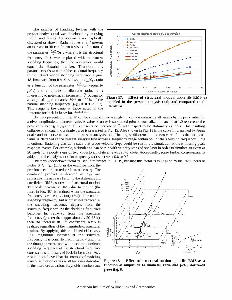
The manner of handling lock-in with the
present analysis tool was developed by studying
Ref. 9 and noting that lock-in is not explicitly
discussed or shown. Rather, Jones et al.9 present
an increase in lift coefficient RMS as a function of
the parameter 𝑓ℎ𝐷
𝑉𝑆𝑡⁄ , where fh is the structural
frequency. If fh were replaced with the vortex
shedding frequency, then the numerator would
equal the Strouhal number. Therefore, this
parameter is also a ratio of the structural frequency
to the natural vortex shedding frequency. Figure
18, borrowed from Ref. 9, shows the �̃�𝐿/�̃�𝐿𝑟 ratio
as a function of the parameter 𝑓ℎ𝐷
𝑉𝑆𝑡⁄ (equal to
fh/fns) and amplitude to diameter ratio. It is
interesting to note that an increase in �̃�𝐿 occurs for
a range of approximately 80% to 120% of the
natural shedding frequency (fh/fns = 0.8 to 1.2).
This range is the same as those noted in the
literature for lock-in behavior.1,6,7,10,11,13
The data presented in Fig. 18 can be collapsed into a single curve by normalizing all values by the peak value for
a given amplitude to diameter ratio. A value of unity is subtracted prior to normalization such that 1.0 represents the
peak value near fh = fns and 0.0 represents no increase in �̃�𝐿 with respect to the stationary cylinder. This resulting
collapse of all data into a single curve is presented in Fig. 19. Also shown in Fig. 19 is the curve fit presented by Jones
et al.9 and the curve fit used in the present analysis tool. The largest difference in the two curve fits is that the peak
value is flattened in the present analysis tool across a frequency range within 5% of the shedding frequency. This
intentional flattening was done such that crude velocity steps could be run in the simulation without missing peak
response events. For example, a simulation can be run with velocity steps of one knot in order to simulate an event at
20 knots, or velocity steps of two knots to simulate an event at 40 knots. Additionally, some further conservatism is
added into the analysis tool for frequency ratios between 0.8 to 0.9.
The term knock-down factor is used in reference to Fig. 19, because this factor is multiplied by the RMS increase
factor at fh = fns (1.75 in the example from the
previous section) to reduce it as necessary. The
combined product is denoted as CLm and
represents the increase factor to the stationary lift
coefficient RMS as a result of structural motion.
The peak increase in RMS due to motion (the
inset in Fig. 18) is retained when the structural
frequency is close in vicinity (5%) to the natural
shedding frequency, but is otherwise reduced as
the shedding frequency departs from the
structural frequency. As the shedding frequency
becomes far removed from the structural
frequency (greater than approximately 20-25%),
then no increase in lift coefficient RMS is
realized regardless of the magnitude of structural
motion. By applying this combined effect as a
PSD magnitude increase at the structural
frequency, it is consistent with items 4 and 7 in
the thought process and will place the dominant
shedding frequency at the structural frequency
consistent with observed lock-in behavior. As a
result, it is believed that this method of modeling
structural motion captures all behavior described
in the literature at various Reynolds numbers and
Figure 17. Effect of structural motion upon lift RMS as
modeled in the present analysis tool; and compared to the
literature.
Figure 18. Effect of structural motion upon lift RMS as a
function of amplitude to diameter ratio and fh/fns; borrowed
from Ref. 9.

American Institute of Aeronautics and Astronautics
12
flow characteristics within the frequency domain. In the present
analysis tool, CLm is calculated for each structural frequency
(mode) of concern.
The quantity of CLm also serves as an indicator of when a
structural mode is experiencing resonant WIO for a given
vehicle station. If CLm is equal to 1.0, then no increase factor is
being applied to the lift coefficient standard deviation, and there
is no effect of structural motion. If CLm is greater than 1.0, then
aeroelastic coupling exists and structural motion is increasing
the local value of lift coefficient standard deviation.
F. Conversion to the Time Domain, Stage 4
Conversion to the time domain is accomplished by the use
of a Fourier series with 1000 components at various frequencies.
The coefficient proceeding each sine wave component is
determined as the square root of the PSD magnitude for the
corresponding frequency multiplied by the dimensional
frequency step size. This product is equal to the square root of
the area under the PSD curve for each frequency component.
The most difficult feature to reconcile in the conversion to a time domain is modeling the phase of each component
of the Fourier series. All of the other steps discussed thus far in this paper are either mathematically computed or
anchored in published data. Phase, however, is more elusive. In theory, there are an infinite number of different time-
domain realizations from a single PSD, all with varying values of phase but otherwise identical components. In the
development of the present analysis tool, phase was extensively experimented with by investigating constant phase
distributions, Gaussian distributions, sinusoidal distributions, linear distributions, and random distributions for the
various frequency components. Most of these models resulted in wild beating of the lift force as frequencies would
coincide and then compete throughout the time history. By far, the most consistent and realistic results were obtained
when using a random phase distribution for the discrete two-dimensional stations.
With the two-dimensional solution determined, the next challenge was then modeling phase-correlation on a three-
dimensional structure. Consider first a cylinder of constant diameter in uniform flow. In this example, the shedding
frequency (fns) will be the same for each vehicle station, and the dimensional values of frequency will be the same.
For the first vehicle station, the values of phase are randomly distributed across the 1000 components of the Fourier
series. For each subsequent vehicle station, the identical phase distribution is used until the correlation length (LC) is
reached, where LC was presented in Fig. 10. For vehicles with changing diameter and/or in the presence of a wind
profile boundary layer, fns is different for each station and the dimensional frequencies will be different. Therefore,
the specified phase distribution will be uncorrelated between any two vehicle stations with a different value of fns.
Using this method of random phase distribution, the analysis tool produced results that agreed well with experimental
non-resonant WIO response. However, consistent with items 1 through 4 of the thought process, the need exists to
also correlate phase during resonant WIO events with significant structural motion regardless of where it occurs on
the vehicle.
In order to selectively correlate phase as required, a method of developing a frequency-based phase map was
established. To accomplish this, the minimum and maximum possible values of fns are calculated for a given free-
stream velocity. A randomly distributed phase “map” is then established as a function of frequency between the values
of zero to twice the value of fns(max). The difference between fns(min) and fns(max) is used to determine an intelligent
number of map steps such that adequate resolution is provided without creating unnecessarily large matrices. With the
establishment of a frequency-based phase map, the ability exists to selectively correlate any component (frequency)
of the Fourier series for a given vehicle station with a component of the same frequency on any other vehicle station,
even if the values of fns are different resulting in different Fourier component index values for the same frequency.
Selection of correlated phase-mapping is limited to conditions where the natural shedding frequency is within
approximately 20 to 25% of a structural frequency that is undergoing significant motion consistent with lock-in
behavior. Within the analysis tool, this condition is determined by CLm for any mode being greater than 1.01 for the
vehicle station. With this ability to selectively correlate phase, the present analysis tool produces results that agree
well with both resonant and non-resonant WIO response data.
An example of selectively correlated phase is presented in Fig. 20 for mode Y2 (second bending mode along the
y-axis that has a frequency of 0.96 Hz) of the Ares I-X. The image to the left contains the values of CLm for each mode
at the various vehicle stations where station zero represents the vehicle base. For reference, a sketch of the Ares I-X
Figure 19. Knock-down factor as modeled in
the present analysis tool.
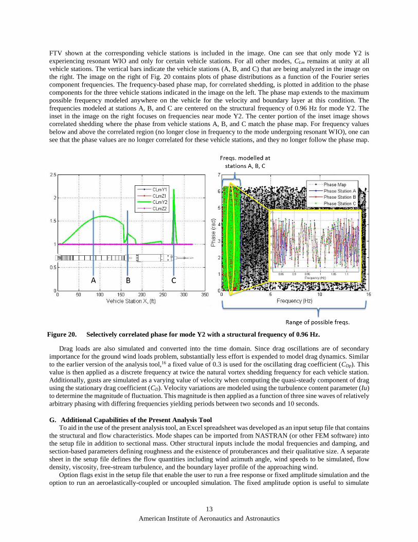
American Institute of Aeronautics and Astronautics
13
FTV shown at the corresponding vehicle stations is included in the image. One can see that only mode Y2 is
experiencing resonant WIO and only for certain vehicle stations. For all other modes, CLm remains at unity at all
vehicle stations. The vertical bars indicate the vehicle stations (A, B, and C) that are being analyzed in the image on
the right. The image on the right of Fig. 20 contains plots of phase distributions as a function of the Fourier series
component frequencies. The frequency-based phase map, for correlated shedding, is plotted in addition to the phase
components for the three vehicle stations indicated in the image on the left. The phase map extends to the maximum
possible frequency modeled anywhere on the vehicle for the velocity and boundary layer at this condition. The
frequencies modeled at stations A, B, and C are centered on the structural frequency of 0.96 Hz for mode Y2. The
inset in the image on the right focuses on frequencies near mode Y2. The center portion of the inset image shows
correlated shedding where the phase from vehicle stations A, B, and C match the phase map. For frequency values
below and above the correlated region (no longer close in frequency to the mode undergoing resonant WIO), one can
see that the phase values are no longer correlated for these vehicle stations, and they no longer follow the phase map.
Drag loads are also simulated and converted into the time domain. Since drag oscillations are of secondary
importance for the ground wind loads problem, substantially less effort is expended to model drag dynamics. Similar
to the earlier version of the analysis tool,16 a fixed value of 0.3 is used for the oscillating drag coefficient (CDp). This
value is then applied as a discrete frequency at twice the natural vortex shedding frequency for each vehicle station.
Additionally, gusts are simulated as a varying value of velocity when computing the quasi-steady component of drag
using the stationary drag coefficient (CD). Velocity variations are modeled using the turbulence content parameter (Iu)
to determine the magnitude of fluctuation. This magnitude is then applied as a function of three sine waves of relatively
arbitrary phasing with differing frequencies yielding periods between two seconds and 10 seconds.
G. Additional Capabilities of the Present Analysis Tool
To aid in the use of the present analysis tool, an Excel spreadsheet was developed as an input setup file that contains
the structural and flow characteristics. Mode shapes can be imported from NASTRAN (or other FEM software) into
the setup file in addition to sectional mass. Other structural inputs include the modal frequencies and damping, and
section-based parameters defining roughness and the existence of protuberances and their qualitative size. A separate
sheet in the setup file defines the flow quantities including wind azimuth angle, wind speeds to be simulated, flow
density, viscosity, free-stream turbulence, and the boundary layer profile of the approaching wind.
Option flags exist in the setup file that enable the user to run a free response or fixed amplitude simulation and the
option to run an aeroelastically-coupled or uncoupled simulation. The fixed amplitude option is useful to simulate
Figure 20. Selectively correlated phase for mode Y2 with a structural frequency of 0.96 Hz.

American Institute of Aeronautics and Astronautics
14
constrained wind-tunnel models such as that used in Ref. 9. In such cases, the aerodynamic forces are calculated for
the fixed amplitude and can be compared to measured forces. Similarly, the aeroelastically-uncoupled simulation has
value since it enables the isolation of aeroelastic effects versus turbulence effects, and it will also band the minimum
expected response for a given flow condition.
VI. Comparison with Experimental Data
A comprehensive comparison is underway to quantify the ability of the analysis tool to model a wide range of
vortex shedding phenomena for various Reynolds numbers, structural shapes, and approaching flow conditions.
Results of this comparison will be used to validate the methodology and architecture of the present analysis tool. A
significant portion of this effort is complete and is presented in this section.
An important observation is that there tends to be significant scatter in most experimental data with regards to the
GWL problem as noticed by inspection of Figs. 18 and 19. This is typical of many experiments and the objective of
GWL analyses is to determine representative peak loads and the corresponding flow conditions in order to provide
guidance for design and operational wind placards. Even in carefully controlled wind-tunnel environments that
simulate two-dimensional flow on simple cylindrical structures, there can be substantial scatter in the data. Therefore,
the user should not expect to replicate exact experimental results with analysis.
A. Two-Dimensional Cylinder at Very High Reynolds Number with Fixed Displacement
To verify the methodology of the present analysis tool, an examination of the input coefficients was conducted
utilizing the configuration and data from Ref. 9 acquired at Reynolds numbers in the vicinity of 5 x10⁶ to 15 x106.
The fixed amplitude option was run to simulate the test conditions from Ref. 9 with an amplitude to diameter ratio of
0.0278. For this amplitude, the value of �̃�𝐿/�̃�𝐿𝑟 should peak at 2.58 for narrow-band shedding when the value of
(fhD/V)/St approaches unity (the structural and natural shedding frequencies match). Figure 21 contains various plots
of the ratio of �̃�𝐿/�̃�𝐿𝑟. The curve denoted as the “target CL ratio” represents the explicitly-defined curves shown in the
inset of Fig. 18 and Fig. 19 derived from narrow-band data of Ref. 9. The curve denoted as “target PSD ratio” is
derived by calculating the square root of the area under the PSD curve with motion, normalized by the square root of
the area of the PSD curve without motion. Finally, the curve denoted as “actual CL ratio” is derived by calculating the
standard deviation of the time-history value of the resulting lift coefficient normalized by the standard deviation of
the lift coefficient for a stationary cylinder. The latter two curves are calculated quantities from the frequency domain
and time domain representation of the lift coefficient within the analysis tool, respectively. Therefore, the slight
variation in values, as seen in the inset of Fig. 21, is expected. Finally, the data from Ref. 9 used to create the target
CL ratio at this amplitude to diameter ratio is included in Fig. 21.
In Fig. 21, the target PSD ratio curve should match the target CL ratio curve for conditions with narrow-band vortex
shedding as modeled in this simulation at this high Reynolds number. Since these curves do match, this validates the
methodology of manipulating the PSD curve in
the frequency domain to produce a target
increase to the standard deviation (RMS for zero
mean) value of the lift coefficient. Similarly, the
target PSD ratio and actual CL ratio curves should
match. Since they do, this confirms that the
conversion to the time domain using a Fourier
series has produced a lift coefficient with the
desired dynamic strength.
Since the model of Ref. 9 was forced at fixed
amplitude, comparing displacement between
analysis and experiment is trivial. The only
validation that can be done is the replication of
the appropriate �̃�𝐿 value as demonstrated in Fig.
21. Not surprisingly, the comparison is nearly
identical to the target curve since Ref. 9 data was
used as the basis for the present analysis tool.
The wind-tunnel model used in Ref. 9 was of
constant diameter, was forced laterally such that
all stations realized the same displacement, and
the aspect ratio satisfied the correlation length
Figure 21. Ratio of �̃�𝑳/�̃�𝑳𝒓 target value, target value
calculated from PSD, actual value calculated from time
history.

American Institute of Aeronautics and Astronautics
15
parameter (Fig. 11) such that the flow should
indeed be two dimensional. Therefore, the phase
of the Fourier series components should be the
same for any station of the vehicle. Figure 22
contains plots of the phase distribution of the
Fourier components for three model stations A,
B, and C representing the base, the middle, and
the top, respectively. All three stations realize the
same phase distribution (and displacement
amplitude). Similarly, Fig. 23 contains a plot of
the lift coefficient for the resonant condition of
(fhD/V)/St = 1. All three vehicle stations are
producing identical lift coefficient time histories
indicative of two-dimensional flow.
B. Two-Dimensional Cylinder at Very Low
Reynolds Number with Free Response
Substantially far removed from the Reynolds
number regime used as a basis for the present
analysis tool, is the data from Ref. 15 acquired at
Reynolds numbers in the vicinity of 6000. There is
uncertainty in the lift coefficient RMS for
stationary cylinders at very low Reynolds numbers
due to substantial differences in the literature from
different experiments.6-11,13,15 Therefore, any
analysis will have some additional uncertainty in
this very low Reynolds number regime.
The data from Ref. 15 was acquired with a two-
dimensional cylinder in smooth uniform flow. The
wind-tunnel model was free response such that the
amplitudes can be compared between experiment
and analysis. The physical dimensions and
frequencies of the model were simulated in the
present analysis tool, and the correlation length
parameter was again satisfied (Fig. 10) such that
the shedding was indeed modeled as two-dimensional.
The ESDU analysis method of Ref. 7 was also
compared to the data from Ref. 15. A comparison of
both analyses and the data are presented in Figs. 24
and 25 for structural damping ratios (ratio with
respect to critical) of 0.00149 and 0.00301,
respectively. The abscissa is a non-dimensional
velocity where the velocity is normalized by structural
frequency and diameter.
The ESDU analysis method is primarily compared
to wind-tunnel data of subcritical Reynolds number
such as those shown in Figs. 24 and 25, and it is likely
that the ESDU analysis method was developed using
the trends observed in this Reynolds number range.
The curves in Fig. 3, representing the effect of motion
upon lift coefficient RMS, would also suggest that the
ESDU analysis method is indeed anchored in data at
the subcritical and transcritical2 Reynolds number
range. Therefore, it would be expected to do very well
at predicting the events that it is most likely anchored
in.
Figure 22. Phase distribution of Fourier series components.
Figure 23. Lift coefficient.
Figure 24. Peak response comparison at very low Reynolds
number, ζ = 0.00149, present analysis tool, ESDU analysis,7
and data.15

American Institute of Aeronautics and Astronautics
16
However, for the launch vehicle problem,
Reynolds numbers are typically supercritical2
(higher than 3 x10⁶). The present analysis tool is
anchored in supercritical data that exhibits
substantially different behavior. Comparison of the
ESDU analysis results and supercritical data is
reserved to full-scale comparisons only due to the
difficulty of the ESDU team to utilize wind tunnels
capable of these higher Reynolds numbers.7 When
analyzing the comparison of ESDU analysis to full-
scale data at this supercritical range, the correlation
ranges from 20% difference to greater than a factor
of three.7 Current work is underway to perform
analyses of these same full-scale events with the
present analysis tool; however, the required
structural properties to enable a comparison have
not yet been found. It should also be noted that
comparisons to full-scale data always involve
greater uncertainty in that the flow velocities,
boundary layer profiles, and turbulence content are
at best estimated using measured conditions from a
few scattered locations. Additionally, full-scale
values of structural damping are substantially more difficult to acquire. Therefore, comparison of analysis results to
full-scale data for the GWL problem is expected to show worse correlation, and it is difficult to evaluate the ESDU
analysis method for applicability to the launch vehicle problem.
The ability of the present analysis tool to predict the response as well as it did in the subcritical Reynolds number
regime (far removed from where it was optimized) lends confidence to the architecture of the analysis tool and the
unique method of modeling structural motion effects within the PSD. Recall from Fig. 3 that motion effects presented
by Jones et al.9 are a factor of approximately 2.4 greater than those shown for the ESDU method. However, the present
analysis tool predicts the peak response magnitude to within 20 percent in Fig. 24 and to within one percent in Fig.
25. Additionally, the velocity of peak response is matched in Fig. 24, and is off by only five percent in Fig. 25.
Consistent with the data from Ref. 9, the data from Ref. 15, and the ESDU analysis,7 the velocity range of peak
response is narrower for increased damping within the present analysis tool. However, contrary to Ref. 9 data, the
ESDU analysis7 shows a shift in peak velocity for
different values of damping. Refs. 7 and 15 attribute
this to the narrowing of the lock-in range where the
onset velocity remains fixed. The data acquired from
Ref. 15 exhibits variations in the value of Vh/FD
where peak response occurs, however, the data
included in Fig. 25 is that utilized by Ref. 7 where it
aligns best with the ESDU analyis.7,15 This shift in
frequency with varying values of damping, or
amplitude, is not observed in Ref. 9 data. At
supercritical Reynolds number, this behavior does not
appear to manifest and is therefore not modeled in the
present analysis tool. Not surprisingly, the analysis
tool does not model this behavior for the subcritical
comparison.
For comparison to the �̃�𝐿/�̃�𝐿𝑟 ratio curves shown
in Fig. 21 (high Re), these same curves are presented
in Fig. 26 for this very low Reynolds number case. At
this Reynolds number, the vortex shedding
bandwidth is broader and the target PSD ratio is of
less magnitude than the narrow-band target derived
from Ref. 9 data. This characteristic of the present
Figure 25. Peak response comparison at very low Reynolds
number, ζ = 0.00301, present analysis tool, ESDU analysis,7
and data.15
Figure 26. Ratio of �̃�𝑳/�̃�𝑳𝒓 target value, target value
calculated from PSD, actual value calculated from time
history; low Reynolds number wide-band.
American Institute of Aeronautics and Astronautics
17
analysis tool enables the reasonable comparison presented in Figs. 24 and 25 while retaining reasonable comparison
in the supercritical Reynolds number regime.
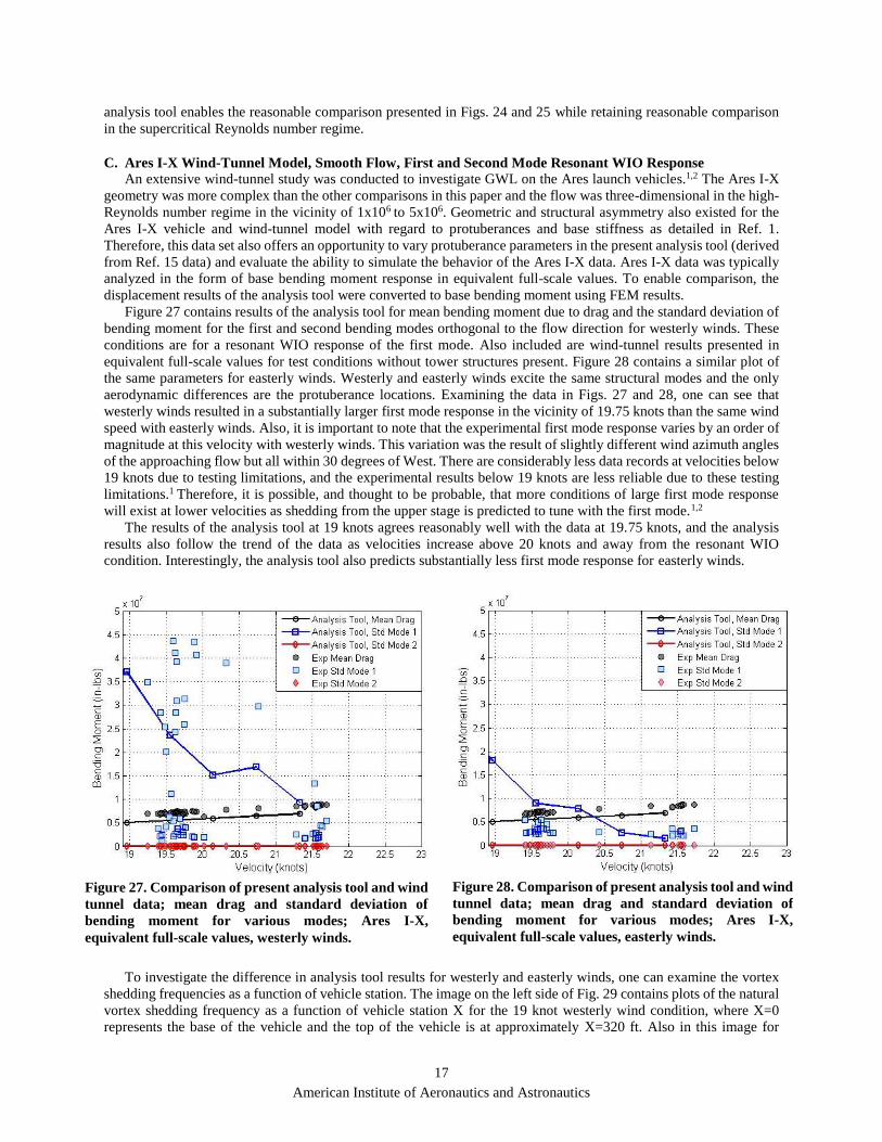
C. Ares I-X Wind-Tunnel Model, Smooth Flow, First and Second Mode Resonant WIO Response
An extensive wind-tunnel study was conducted to investigate GWL on the Ares launch vehicles.1,2 The Ares I-X
geometry was more complex than the other comparisons in this paper and the flow was three-dimensional in the high-
Reynolds number regime in the vicinity of 1x10⁶ to 5x10⁶. Geometric and structural asymmetry also existed for the
Ares I-X vehicle and wind-tunnel model with regard to protuberances and base stiffness as detailed in Ref. 1.
Therefore, this data set also offers an opportunity to vary protuberance parameters in the present analysis tool (derived
from Ref. 15 data) and evaluate the ability to simulate the behavior of the Ares I-X data. Ares I-X data was typically
analyzed in the form of base bending moment response in equivalent full-scale values. To enable comparison, the
displacement results of the analysis tool were converted to base bending moment using FEM results.
Figure 27 contains results of the analysis tool for mean bending moment due to drag and the standard deviation of
bending moment for the first and second bending modes orthogonal to the flow direction for westerly winds. These
conditions are for a resonant WIO response of the first mode. Also included are wind-tunnel results presented in
equivalent full-scale values for test conditions without tower structures present. Figure 28 contains a similar plot of
the same parameters for easterly winds. Westerly and easterly winds excite the same structural modes and the only
aerodynamic differences are the protuberance locations. Examining the data in Figs. 27 and 28, one can see that
westerly winds resulted in a substantially larger first mode response in the vicinity of 19.75 knots than the same wind
speed with easterly winds. Also, it is important to note that the experimental first mode response varies by an order of
magnitude at this velocity with westerly winds. This variation was the result of slightly different wind azimuth angles
of the approaching flow but all within 30 degrees of West. There are considerably less data records at velocities below
19 knots due to testing limitations, and the experimental results below 19 knots are less reliable due to these testing
limitations.1 Therefore, it is possible, and thought to be probable, that more conditions of large first mode response
will exist at lower velocities as shedding from the upper stage is predicted to tune with the first mode.1,2
The results of the analysis tool at 19 knots agrees reasonably well with the data at 19.75 knots, and the analysis
results also follow the trend of the data as velocities increase above 20 knots and away from the resonant WIO
condition. Interestingly, the analysis tool also predicts substantially less first mode response for easterly winds.
To investigate the difference in analysis tool results for westerly and easterly winds, one can examine the vortex
shedding frequencies as a function of vehicle station. The image on the left side of Fig. 29 contains plots of the natural
vortex shedding frequency as a function of vehicle station X for the 19 knot westerly wind condition, where X=0
represents the base of the vehicle and the top of the vehicle is at approximately X=320 ft. Also in this image for
Figure 27. Comparison of present analysis tool and wind
tunnel data; mean drag and standard deviation of
bending moment for various modes; Ares I-X,
equivalent full-scale values, westerly winds.
Figure 28. Comparison of present analysis tool and wind
tunnel data; mean drag and standard deviation of
bending moment for various modes; Ares I-X,
equivalent full-scale values, easterly winds.

American Institute of Aeronautics and Astronautics
18
reference are the frequency of the first mode in the North-South “Z-direction” and a sketch of the Ares I-X FTV shown
at the corresponding vehicle stations. The image on the right side of Fig. 29 contains plots of the value of CLm for the
various modes. One can see in the plot on the left that the natural shedding frequency is very close to the structural
frequency at the top of the upper stage (vicinity of X=250 ft) and around the tip of the command module (vicinity of
X=270 ft). Figure 30 contains similar plots as Fig. 29, but for the easterly wind condition. In Fig. 30, one can see that
the natural shedding frequency of the upper stage is further removed from the natural frequency. The Ares I-X contains
a system tunnel on the upper stage on the West-hand side and a small liquid hydrogen feed line on the lower portion
of the upper stage on the East-hand side. The systems tunnel is in the wake of the vehicle for easterly winds and the
effects of this protuberance are not modeled in the analysis tool for easterly winds, whereas they are for westerly
winds. Therefore, the analysis tool offers an explanation for the order of magnitude difference in peak response
observed in the wind tunnel. It is likely that the tip shedding phenomena experienced lock-in at the same westerly
flow condition where the upper portion of the upper stage also experienced lock-in. The present analysis tool also
predicts slight resonant WIO response for easterly winds due to tip-shedding; however, the wind-tunnel results do not
exhibit resonant WIO. It is possible that this condition could manifest if additional flow azimuth angles and speeds
were tested in the wind tunnel. It is also possible that a strong response similar to the westerly winds could be
experienced with different boundary layer profiles and easterly winds.
Figure 29. Relation of vortex shedding frequencies and structural frequency of mode Z1, and resulting CLm; Ares
I-X, westerly winds.
Figure 30. Relation of vortex shedding frequencies and structural frequency of mode Z1, and resulting CLm; Ares
I-X, easterly winds.
CL
m
CL
m

American Institute of Aeronautics and Astronautics
19
It is noteworthy that tip shedding predictions with a complex tip geometry is especially uncertain since the
relationships are derived from linearly-tapered structures. The ability of the present analysis tool to capture the peak
response amplitude to within 15 percent and the resonant velocity to within four percent is considered reasonable
given this particularly difficult tip-shedding simulation task.
In addition to the analysis of vortex shedding effects, drag is under-predicted by the present analysis tool. This is
expected since protuberance effects are not yet
modeled in the calculation of drag. Therefore, the mean
drag results from the analysis tool should be
representative of a clean vehicle with no protuberances.
A large second mode resonant WIO response was
encountered in the wind tunnel for northerly and
southerly winds at a velocity of approximately 33
knots. Figure 31 contains results of the analysis tool
compared to experimental data for southerly winds.
The analysis tool predicts a strong second mode peak
at 34 knots of nearly identical magnitude and trends.
The analysis tool also has reasonable agreement with
the dynamics of the modes for non-resonant WIO
conditions. This second mode response is the condition
previously presented in Fig. 20 where the dominant
response results from first-stage shedding near the
second mode anti-node.
The ability of the present analysis tool to capture
the second mode response magnitude is of great
importance. This event could produce the most critical
loads for the Ares I-X,2 and the analysis tool predicted
the peak magnitude to within two percent of the
experimental data and the corresponding resonant
velocity to within five percent.
D. Ares I-X Wind-Tunnel Model, Structure-Turbulence, Non-Resonant First Mode Response
During wind-tunnel testing of the Ares I-X, the
influence of the launch pad tower structure on GWL was
also investigated. For many of these conditions, the
wind-tunnel model experienced significantly more
response consistent with other launch vehicle studies.4,5
Refs. 4 and 5 attribute the increase in response to wake
turbulence from the surrounding tower structures. Ares
I-X wind-tunnel data were examined for a case of
westerly winds that would place the vehicle leeward of
the tower structure. The standard deviation of the base
bending moment due to drag were normalized by the
mean to derive an estimate of the value of free-stream
turbulence impacting the vehicle model. This derivation
resulted in an estimate of the free stream turbulence
impacting the vehicle model to be approximately eight
percent; however, the appropriate value is not known a
priori. By comparison, nominal tunnel flow turbulence at
this condition is approximately one-half percent. The
analysis tool was run with a turbulence content
parameter of eight percent and compared to the wind-
tunnel data. Figure 32 contains the results of this
comparison. The response values of the first mode from
the present analysis tool match reasonably well with the
scatter of experimental data. It should be noted that this condition is a non-resonant WIO response and it resulted in
Figure 31. Comparison of present analysis tool and wind
tunnel data; mean drag and standard deviation of bending
moment for various modes; Ares I-X, equivalent full-scale
values, Southerly winds.
Figure 32. Comparison of present analysis tool and wind
tunnel data; mean drag and standard deviation of bending
moment for various modes; Ares I-X, equivalent full-scale
values, westerly winds leeward of structure.

American Institute of Aeronautics and Astronautics
20
dynamic load magnitudes of approximately 1.5 to 2.0 times larger than those acquired in nominal flow without tower
structures present.
E. Ares I-X FTV, Atmospheric Turbulence, Non-Resonant First Mode Response
During rollout to the pad, the full-scale Ares I-X FTV was
exposed to negligible winds. After arrival at the pad and prior
to capture of an extended-stay damper, there was a period of
notable, yet non-resonant, WIO response. This event is
described in greater detail in Ref. 2. Wind-tunnel data for a
similar configuration and approaching flow angle was acquired
in smooth flow. Since this condition is a non-resonant WIO,
the dynamic response of the wind-tunnel model in smooth flow
was less than the full-scale FTV in turbulent flow as expected.
Wind anemometer readings in the vicinity of the launch pad
were analyzed to estimate the wind velocity, turbulence
content, and wind boundary layer profile at the time of the full-
scale data record.2 A comparable simulation was run within the
present analysis tool for the same value of turbulence content
(18 percent) and a nominal (0-sigma) wind boundary layer
profile as recommended by climatic guidelines for the
Kennedy Space Center.20 With this wind profile simulation, the
reference height velocity should be in the vicinity of 19 to 21
knots. Figure 33 contains a plot of the analysis tool results
compared to the full-scale data. Similar to wind-tunnel
comparison, the drag is under predicted, as expected, since
protuberance effects are not accounted for in the drag
calculations. Additionally, the full-scale values of drag and
standard deviation of the first-mode bending moment are
plotted as a constant value across the range of velocity values
shown in this plot since there is uncertainty in the exact
atmospheric conditions during acquisition of the full-scale data
record.2 The results of the analysis tool match reasonably well
with the measured dynamic response of the full-scale vehicle.
For comparison, the wind-tunnel results of the most
representative flow condition are also included in Fig. 33, and plotted as a constant value across the range of velocity
values. With uniform flow in the wind tunnel, the most representative condition was acquired at an equivalent full-
scale velocity of 25.5 knots and yields similar drag loads to that acquired by the full-scale vehicle with a reference-
height velocity of 19 to 21 knots and an estimated 0-sigma wind boundary layer profile.20
F. Additional Comments about Comparison with Experimental Data
The ability of the present analysis tool to reasonably match measured data for a broad range of turbulence levels
lends confidence in the tool to model free-stream turbulence effects. Furthermore, the present analysis tool has
reasonably matched all resonant WIO response magnitudes and resonant velocities observed in the wind-tunnel data
used for comparison acquired at various Reynolds numbers. Work is currently underway to conduct comparisons
between the analysis tool and additional experimental results such as those found in Ref. 7. However, many of these
experimental results were acquired in the transcritical2 range of Reynolds number where there is great uncertainty in
Strouhal number, shedding bandwidth, and lift coefficient RMS, and reasonable correlation will depend upon the data
set selected for comparison.
British mathematician and statistics professor George Box stated that “all models are wrong, but some are useful”
in his work regarding empirical methods and statistics.22 In the use of analysis tools for the launch vehicle GWL
problem, the purpose of the analysis must be remembered. The purpose of GWL analyses and testing efforts is to
identify the atmospheric conditions were large WIO response may occur, to predict the peak response loads for a range
of flow conditions, to help develop operational placards, and to identify sensitivities between vehicle design and flow
characteristics and GWL response. The present analysis tool provides useful information at a low cost enabling many
predictions in a short period of time.
Figure 33. Comparison of present analysis tool and
full-scale data; mean drag and standard deviation
of bending moment; Ares I-X, Easterly winds
windward of structure.

American Institute of Aeronautics and Astronautics
21
VII. Future Work
Work is currently underway to conduct a comparison to full-scale first mode and second mode resonant WIO
responses to validate the simulation of structural motion while exposed to broadband highly-turbulent flow. Data of
this nature are not available in the literature since great efforts are typically expended to avoid such an occurrence on
full-scale vehicles. Understandably, launch vehicle operators are unwilling to have an accident in order to validate
wind-tunnel or analytical methodology. Recent acquisition of this full-scale resonant WIO data in a turbulent
atmosphere enables unique comparison.
Future work will also seek to optimize the number of Fourier series components and the range of frequencies
modeled in the PSD. Reducing the number of Fourier series components will lessen the variations in peak response
magnitude for slightly different flow conditions. It is desirable to reduce variations but not to the extent that meaningful
content is lost. Additionally, increasing the range of PSD frequencies beyond the current range of twice the vortex
shedding frequency may improve non-resonant WIO response correlation.
Other future work is intended to model atmospheric gusts with either a Dryden or von Kármán turbulence model.
With such a model, drag loads are intended to be simulated similar to the lift loads in order to yield more representative
drag oscillations and response to atmospheric gusts. Since drag oscillations are of secondary importance in the ground
wind loads problem, the current methodology of modeling drag is considered adequate for producing meaningful
results.
Additionally, modeling the effect of fuel slosh is planned for future work. The preliminary concept is to model the
fuel weight with a damped pendulum mounted to the structure. The length of the pendulum arm will be determined
by fuel tank geometry and fuel state.
Finally, consideration will be given to the integration of probability theory with respect to the present analysis tool.
The analysis tool is stochastic in nature due to the random distribution of phase. Therefore, the same conditions can
be simulated with the same vehicle characteristics and some variations will exist in the results. Additionally, variations
in the modeling of protuberance and tip effects are recommended for future launch vehicle analyses since slight
changes to these parameters can have notable effects on the results.
VIII. Concluding Remarks
Launch vehicles are exposed to ground winds during rollout and on the pad prior to launch that can induce static
and dynamic loads. Of particular concern are the dynamic loads caused by vortex shedding from nearly-cylindrical
structures. The current state-of-the-art in modeling and predicting vortex shedding loads has been presented showing
the difficulty in accurately doing so and the need for the present analysis tool.
The present analysis tool was developed to fill the analytical capability gap and estimate launch vehicle response
to ground wind loads. This tool is designed to simulate the dynamic response resulting from wind induced oscillations
(WIO) and is optimized for the Reynolds number range of interest to launch vehicles. Unlike many other analysis
methods, the present analysis tool is of general form and applicable to any single-body structure of nearly cylindrical
shape. Wake from nearby truss-like structures can be simulated as broadband turbulence content of the approaching
flow. To utilize the tool, the user specifies vehicle characteristics including geometry, surface roughness, protuberance
locations, mode shapes, modal frequencies, and damping; and flow characteristics including wind azimuth and speed,
wind boundary-layer profile, density, viscosity, and free-stream turbulence content. The vehicle under analysis is then
discretized into multiple two-dimensional vehicle stations.
To derive the aerodynamic loads for each station of the vehicle, the analysis tool progresses through four stages.
In the first stage, coefficients are calculated based upon flow and vehicle properties (corrected for tip effects) and an
assumed displacement amplitude for each mode. In the second stage, these coefficients are used to derive a
representation of the lift coefficient in the frequency domain. In the third stage, the effects of structural motion are
modeled in the frequency domain. Finally, in the fourth stage, the aerodynamic forces are converted into the time
domain.
At the conclusion of the four stages, the process is repeated for each station of the vehicle until time-domain forces
are determined along the full length of the vehicle. These full-length forces are then multiplied by the mass-normalized
mode shapes and a state-space, time-marching, Runge-Kutta routine is solved. Upon completion of the Runge-Kutta
routine, the newly calculated displacement amplitudes are compared with the original assumed displacement
amplitudes. Coefficients are updated accordingly and the initial conditions of the structure are adjusted. An iterative
loop is then completed until the displacement amplitudes of each mode are converged to within one percent.
Details regarding the operation of the code have been presented to include pertinent equations. Results of the
analysis tool have been presented and compared with experimental data acquired at various Reynolds numbers. The
analytical results compare reasonably well to both resonant WIO and non-resonant WIO wind-tunnel data acquired at

American Institute of Aeronautics and Astronautics
22
low and high Reynolds numbers and at various levels of free-stream turbulence. The present analysis tool also
compares well with full-scale non-resonant WIO data acquired in a turbulent atmosphere at high Reynolds number.
A comprehensive comparison of the present analysis tool results to additional experimental data from various
Reynolds numbers and geometric shapes is currently underway.
Finally, plans for future work were presented that include a comparison of the analysis tool results with full-scale
resonant WIO data acquired in a turbulent atmosphere; a truly unique data set and comparison opportunity.
References 1Keller, D. K., and Ivanco, T. G., “Wind-tunnel Investigation of Ground Wind Loads for Ares Launch Vehicle,” 28th AIAA
Applied Aerodynamics Conference, Chicago, IL, AIAA-2010-4371, June 2010. 2Ivanco, T. G., and Keller, D. K., “Investigation of Ground-Wind Loads for Ares Launch Vehicles,” Journal of Spacecraft and
Rockets, Volume 49, No. 4, July-August 2012, pp. 574-585. 3“Prelaunch Ground Wind Loads.” NASA Space Vehicle Design Criteria, NASA SP 8008, November 1965. 4Foughner, J. T., and Duncan, R. L., “A Full-Scale Ground Wind Load Program,” NASA N66-32230, January 1966. 5Runyan, H. L., Morgan, H. G., and Mixson, J. S., “Use of Dynamic Models in Launch-Vehicle Development,” NASA N65-
24114, presented at the 18th Structures and Materials Panel – AGARD, May 1964. 6Chen, Shoei-Sheng., Flow-Induced Vibration of Circular Cylindrical Structures, Hemisphere Publishing Corporation,
Washington, D.C., 1987. 7“Response of Structures to Vortex Shedding.” Structures of Circular or Polygonal Cross Section. Engineering Sciences Data
Unit (ESDU), Report 96030, United Kingdom, December 1996. Amended July 1998. 8Jones, G. W., “Unsteady Lift Forces Generated by Vortex Shedding about a Large Stationary and Oscillating Cylinder at High
Reynolds Numbers,” ASME Symposium on Unsteady Flow, Philadelphia, PA, May 1968, ASME 68–FE–36. 9Jones, G. W., Cincotta, J. J., and Walker, R. W., “Aerodynamic Forces on a Stationary and Oscillating Cylinder at High
Reynolds Number,” NASA TR R-300, February 1969. 10Lienhard, J. H., “Synopsis of Lift, Drag, and Vortex Frequency Data for Rigid Circular Cylinders,” Bulletin 300, Washington
State University, College of Engineering, Research Division, 1966. 11Delany, N. K., and Sorensen, N. E., “Low-Speed Drag of Cylinders of Various Shapes,” NACA TN 3038, November 1953. 12McCullough, G. B., and Steinmetz, W. J., “A Wind-Tunnel Study of Ground-Wind Loads on Launch Vehicles Including the
Effects of Conduits and Adjacent Structures,” NASA TN D-2889, July 1965. 13Roshko, A., “Experiments On the Flow Past a Circular Cylinder at Very High Reynolds Number,” Journal of Fluid
Mechanics, Volume 10, No. 3, 1961, pp. 345 – 356. 14Reed, W.; Models for Obtaining Effects of Ground Winds on Space Vehicles Erected on the Launch Pad. NASA Langley
Research Center. 1964. 15Goswami, I., Scanlan, R. H., Jones, N. P.; “Vortex-Induced Vibration of Circular Cylinders. I: Experimental Data,” Journal
of Engineering Mechanics, Vol. 119, November 1993, pp. 2270-2287. 16Ivanco, T. G., Patil, M., Silva, W. A., Kapania, R. K., “Development and Validation of an Aeroelastic Ground Wind Loads
Analysis Tool for Launch Vehicles,” Master of Science Thesis, Virginia Polytechnic Institute and State University, Blacksburg,
VA, July 2009. 17fun3d.larc.nasa.gov 18Bartels, R. E., Chwalowski, P., Biedron, R. T., Keller, D., “Computational Aeroelastic Simulations Supporting the Ground
Wind Loads Checkout Test,” Internal NASA report, 2009. 19Bartels, R. E., “FUN3d CAE Simulations of the Flexible Ares Crew Launch Vehicle Using the NAS Computing System,”
Super Computing Conference, Austin, TX, 2008. 20Johnson, D. L.; “Terrestrial Environment (Climatic) Criteria Guidelines for Use in Aerospace Vehicle Development, 2008
Revision,” NASA TM 2008-215633, December 2008. 21Szechenyi, E., “Supercritical Reynolds Number Simulation for Tow-Dimensional Flow Over Circular Cylinders,” Journal of
Fluid Mechanics, Vol. 70, Pt. 3, 1975, pp. 529-542. 22Box, G. E. P., Draper, N. R.; Empirical Model Building and Response Surfaces, John Wiley & Sons, New York, NY, 1987.